was there a riverside miracle? an hierarchical framework for

Was There a Riverside Miracle? An HierarchicalFramework for Evaluating Programs with Grouped Data*

Journal of Business and Economic Statistics, Vol. 21, No. 1, pp. 1-11 (January 2003)(previously circulated as NBER Working Paper 7844)

Rajeev Dehejia**

Department of Economics and SIPAColumbia University

andNBER

This paper uses data from the Greater Avenues for Independence (GAIN) demonstration to discuss theevaluation of programs that are implemented at multiple sites. Two frequently used methods are poolingthe data or using fixed effects (an extreme version of which estimates separate models for each site). Theformer approach, however, ignores site effects. Though the latter incorporates site effects, it lacks aframework for predicting the impact of subsequent implementations of the program (e.g., will a newimplementation resemble Riverside or Alameda?). I present an hierarchical model that lies between thesetwo extremes. For the GAIN data, I demonstrate that the model captures much of the site-to-site variationof treatment effects, but has less uncertainty than a model which estimates treatment effects separately foreach site. I also show that uncertainty in predicting site effects is important: when the predictive uncertaintyis ignored, the treatment impact for the Riverside sites is significant, but when we consider predictiveuncertainty, the impact for the Riverside sites is insignificant. Finally, I demonstrate that the model is ableto extrapolate site effects with reasonable accuracy, when the site for which the prediction is being madedoes not differ substantially from the sites already observed. For example, the San Diego treatment effectscould have been predicted based on observable site characteristics, but the Riverside effects are consistentlyunderpredicted.

Key words: Program evaluation, Site effects, Hierarchical modeling

First version: 1 June 1998Current version:11 July 2001

* The author acknowledges support from the Connaught Fund (University of Toronto), and thanks theManpower Demonstration Research Corporation for making available data from the Greater Avenues forIndependence Demonstration. Gary Chamberlain, Siddhartha Chib, Barton Hamilton, Caroline Hoxby,Guido Imbens, Larry Katz, Geert Ridder, Jeffrey Smith, an Associate Editor, an anonymous referee, andseminar participants at Columbia University, Washington University, the Johns Hopkins University, andthe NSF Econometrics and Statistics Symposium on Quasi-Experimental Methods are gratefullyacknowledged for their comments and suggestions.** Department of Economics, Room 1022, Columbia University, 420 W. 118th Street, New York, NY10027. E-mail: [email protected].

1

1. Introduction

This paper discusses the problem of evaluating and predicting the treatment impact of a

program that is implemented at multiple sites; at a methodological level, the paper

illustrates the use of hierarchical models for data that has a group (e.g., site) structure.

Many programs operate, or are evaluated, at multiple sites, e.g., the National Supported

Work Demonstration, Job Training Partnership Act Demonstration, and Greater Avenues

for Independence (GAIN). This paper presents a framework for dealing with multi-site

programs, and (using data from GAIN) argues that it is essential to consider the site

structure of data when evaluating a program.

When data has a site structure, there is a distinction between evaluating a program

and predicting the outcome in subsequent implementations. Evaluation is an historical

question. One wants to determine what the impact of a program was in a particular site at

a particular point in time. Prediction instead relates to future implementations of a

program, either at one or more of the sites where the evaluation was conducted or

possibly at a new site. Both kinds of questions are potentially challenging with multi-site

programs.

The challenge with evaluation is how and to what extent data should be pooled

across sites. Differences across sites can emerge for two reasons. There can be

differences in the composition of participants, which is addressed relatively easily if a

sufficient number of the participants’ characteristics are observed. But there can also be

site-specific variation in the treatment, differences ranging from the services offered to

administrative philosophy. To the extent that site-specific effects are absent and that we

can condition on individual characteristics, the benefit of pooling the data is increased

2

precision in the estimates. This can be particularly important if there are very few

observations at some sites. If site effects are present, the data can still be pooled if we

allow for fixed effects. However, this leads to difficulties in predicting the impact of the

program.

Fixed effects or, more generally, estimating separate models for each site limit us

to thinking of subsequent implementations of the program as being identical to one of the

original sites, because there is no framework to account for predictive uncertainty

regarding the value of the fixed effect or site-specific model. This is true both when

predicting the impact at one of the sites in the evaluation (in which case we want to re-

draw for the site effect) and when predicting the impact at a new site.

The solution that this paper proposes is hierarchical modeling (see Chamberlain

and Imbens [1996], Geweke and Keane [1996], and Rossi, McCulloch, and Allenby

[1995] for other applications of these methods). Hierarchical modeling is a middle-

ground between fixed effects modeling and pooling the data without fixed effects.

Hierarchical modeling is somewhat familiar in the literature through the related concept

of meta-modeling (see Cooper and Hedges [1994]). Meta-modeling involves linking the

outcomes of separate studies on the same topic through an over-arching model. It can

also be used to model site effects; for example, Card and Krueger (1992) estimate cohort

and state-of-birth specific returns to schooling and then use a meta-model to relate these

to measures of school quality. The method adopted in this paper is a Bayesian version of

meta-modeling.

There are three layers to the model: the first involves separate models for each

site; the second links the coefficients of the site models through a regression-type meta-

3

model; and the third consists of prior distributions for the unknown parameters. Thus, an

hierarchical model combines features of the fixed-effect and pooled models, but also

allows for intermediate models. Compared to standard fixed (or random) effects model, it

allows for site-specific estimation of all coefficients, not just the constants. Further,

participants across sites are not assumed to be exchangeable conditional on individual

characteristics, but rather to be exchangeable within sites conditional on individual

characteristics. Finally, we use a prior distribution to model the extent to which we

believe that site-effects are drawn from a common distribution; namely, the extent to

which coefficients should be “smoothed” across sites, or observations from one site

should influence our estimates in other sites.

This approach is applied to data from the GAIN Demonstration, a labor training

program implemented in six California counties at 24 sites (see Riccio, et al., [1996]).

For the GAIN data, the primary benefit of applying hierarchical models is in terms of

prediction rather than evaluation. Each site has a sufficient number of observations so

that the gain in precision from pooling data from other sites is limited. However, the

predictive questions are of central importance. Much attention in the GAIN program

focused on the Riverside county implementation, which was viewed as being highly

successful and distinct from other counties (see, for example, Nelson [1997]).

Our interest is in discovering the extent to which an hierarchical model succeeds in

capturing these site effects which have been viewed as being primarily qualitative in

nature. We focus on three issues. First, does data from other sites help in evaluating the

program at a given site? Second, if we imagine re-implementing a GAIN-type program,

would we be able to predict the site effects based on the observable characteristics of

4

each site, and how important is predictive uncertainty? Third, how well can the model

extrapolate to sites that have not been observed?

Previous papers on multi-site evaluation issues include: Heckman and Smith

(1996), Hotz, Imbens, and Mortimer (1998), and Hotz, Imbens, and Klerman (2000).

Heckman and Smith analyze the sensitivity of experimental estimates to the choice of

sites used in the analysis and to different methods of weighting the pooled data. Their

paper establishes that there is significant cross-site variation in the data from the JTPA

evaluation. Hotz, Imbens, and Mortimer analyze the importance of site effects in the

Work Incentives demonstration using the key insight that, even if there is heterogeneity

in the treatment available at each site, control groups excluded from the treatment still

should be comparable. They find that control group earnings are comparable across sites,

when controlling both for individual characteristics and for site-level characteristics;

however, post-treatment earnings for the treated group earnings are not comparable,

suggesting the existence of heterogeneity in the treatment. Taken together, both papers

motivate the use of an hierarchical model, which allows explicitly for site effects in

treatment and control earnings and directly incorporates site-level characteristics.

Hotz, Imbens, and Klerman is complementary to this paper. It examines the

GAIN data using the same framework as Hotz, Imbens, and Mortimer, and the findings

are also similar. The authors are able to adjust for differences in control group earnings

using individual and site-level characteristics. However, differences remain in post-

treatment earnings. The paper thus presents a series of differences-in-differences

estimates which, inter alia, suggest that the treatment available at Riverside did have a

5

positive effect relative to the treatment offered at other sites. This finding will be

discussed in Section 5.

This paper is organized as follows. Section 2 describes the GAIN program.

Section 3 discusses key features of the GAIN data. Section 4 outlines the hierarchical

model. Section 5 presents the results, and Section 6 concludes.

2. The GAIN Program

The GAIN program began operating in California in 1986, with the aim of “increasing

employment and fostering self-sufficiency” among AFDC recipients (see Riccio, et al.,

[1994]). In 1988, six counties -- Alameda, Butte, Los Angeles, Riverside, San Diego, and

Tulare -- were chosen for an experimental evaluation of the benefits of GAIN. A subset

of AFDC recipients (single parents with children aged six or older and unemployed heads

of two-parent households) were required to participate in the GAIN experiment (see

Table 1). 1

Potential participants from the mandatory group were referred to a GAIN

orientation session when they visited an Income Maintenance office (either to sign up for

welfare or to qualify for continued benefits).2 As a result, the chronology of the data and

subsequent results are in experimental time, rather than calendar time. No sanctions were

used if individuals failed to attend the orientation sessions. However, once individuals

started in the GAIN program, sanctions were used to ensure their ongoing participation.

At the time of enrollment into the program, a variety of background characteristics were

recorded for both treatment and control units including: demographic characteristics;

1 This discussion draws on Dehejia (1999).

6

results of a reading and mathematics proficiency test; and data on ten quarters of pre-

treatment earnings, AFDC, and food stamp receipts.3

Of those who attended the orientation session, a fraction was randomly assigned

to the GAIN program, 4 and the others were prohibited from participating in GAIN.5 Each

of the counties randomized a different proportion of its participants into treatment,

ranging from a 50-50 split in Alameda to an 85-15 split in San Diego (see Table 1).

Because assignment to treatment was random, the distribution of pre-treatment covariates

is balanced across the treatment and control groups. In terms of the chronology of data

gathering, “experimental” time (which I also refer to as “post-experimental” or “post-

treatment” time) begins when individuals attend the GAIN orientation session. The early

stages of experimental time thus coincide with the education and training of GAIN

participants.6

In the GAIN experiment, the treatment is participating in the GAIN program; the

control is receiving standard AFDC benefits. The GAIN program works as follows:

based on test results and an interview with a case manager, participants were assigned to

one of two activities. Those deemed not to be in need of basic education were referred to

a job search activity (which lasts about three weeks); those who did not find work were

2 In some counties AFDC recipients were allowed to volunteer into the GAIN program, but these units arenot included in the public use sample.3 Data on AFDC and Food Stamp receipts were taken from each county’s welfare records. Data onearnings were taken from the California State Unemployment Insurance Earnings and Benefits Records.Other background characteristics were taken from California’s client information (“GAIN-26”) form. SeeRiccio, et al., (1994).4 The randomization was (as far as we know) independent of pre-treatment covariates. This is confirmed bythe data. A different fraction was randomized into treatment in each county. See Table 1.5 Of course, these individuals could participate in non-GAIN employment-creating activities.6 More precisely, individuals were registered in the first quarter of experimental time. This means that insome cases the first quarter of experimental time in fact includes information one or two months prior tothe commencement of the experiment. So for example, for an individual who attended an orientationsession in February 1989, the first quarter of experimental time is from January to March 1989. Of course,

7

placed in job training (which included vocational or on-the-job training and paid or

unpaid work experience, lasting about three to four months). Those deemed to be in need

of basic education could choose to enter job search immediately, but if they failed to find

a job they were required to register for preparation toward the General Educational

Development certificate, Adult Basic Education, or English as a Second Language

programs (lasting three to four months).7 Participants were exempted from the

requirement to participate in GAIN activities if they found work on their own. 8

The counties in the GAIN experiment varied along two important dimensions.

First, the composition of program participants varied, because counties chose to focus on

particular subsets of their welfare populations and the populations differed. For example,

Alameda and Los Angeles counties confined themselves to the subset of long-term

welfare recipients (individuals having already received welfare for two years or more).

The second difference is that the sub-treatment offered within each county varied due to

differences in administrative philosophy. The approach followed by Riverside, which has

received much attention, was to focus on job, rather than skills, acquisition. Both are part

of the program, but Riverside’s emphasis was the former. Instead counties like Alameda

focused more on skill acquisition. The model will allow for differences in composition by

some part of the first and second quarters could be spent participating in treatment activities. Pre-treatmentdata would cover the ten quarters from July 1986 to December 1988.7 The public use data do not contain information on each individual’s participation in the variouscomponents of the program. At the same time, individuals in the control group can participate in non-GAINactivities. Thus, the treatment effect measures the increase in earnings, employment, etc., from theavailability of and encouragement (or requirement) to use GAIN-related activities compared to pre-existingemployment services.8 Note that only about eight-five percent of the treated units actively participated in any GAIN activities(though by virtue of being in the GAIN sample they did attend an orientation meeting); the balancesatisfied the requirements of the GAIN program on their own (in most cases finding employment within thefirst two or three quarters of experimental time). Thus, as observed earlier, this is important in interpretingthe treatment effect as a comparison between earnings, employment, etc., when individuals are required tofind a job or to participate in GAIN-related activities and when they are not obliged to find jobs and onlypre-existing employment-related services are available.

8

conditioning on pre-treatment covariates and differences in the treatment by allowing for

site effects.

3. The GAIN Data

Table 1 presents the six counties that participated in the GAIN experiment, broken down

in terms of their 24 administrative sites. The counties vary from one-site counties such as

Alameda to multi-site counties such as Los Angeles and San Diego. This paper will

analyze the results at the site level because with six counties there is minimal scope for

modeling site effects. Table 2 presents the background characteristics of each site in

greater detail. We note that the average number of children varies from over four in some

sites (site 21) to slightly over two in others (site 6). The proportion of Hispanics in the

sample varies from a low of 6 percent (site 1) to over 50 percent in other sites (sites 14

and 24).

Table 2 shows that there is significant variation in the treatment impact across

sites. The second-last row presents the average quarterly post-treatment earnings for the

treatment and control groups. The treatment impact ranges from a high of $212 for Site 5

(in Riverside county) to a low of –$132 for Site 17 (in Tulare). In the last row the

treatment effect is estimated conditioning on pre-treatment covariates through an OLS

regression. The estimates are similar, ranging from –$90 to $292. The sites consistently

showing the highest and most significant impacts are those from Riverside county (sites 2

to 5). Their treatment impacts range from $149 to $292, and are significantly different

from zero. The worst performing county is Tulare, for which some of the impacts are

negative and all are statistically insignificant.

9

4. The Econometric Model

An important feature of the data which influences the modeling strategy is the large

proportion of zeros in the outcome, earnings. With as many as 75 percent of the outcomes

being zero, the model must explicitly account for the mass point in the earnings

distribution. The most parsimonious model for dealing with a mass point at zero is the

Tobit model.

4.1 The Hierarchical Model

The hierarchical model (see Gelman, Carlin, Stern, and Rubin [1996]) is a generalization

of the regression model that allows each site to have its own value for the coefficients:

{ } ),'(~, 22,,

* σβσβ itjjjjtiitjitj xNxY∀

, (1)

where Yijt is observed income and Y*ijt is a latent variable such that Yijt=0 if Y*

ijt<0 and

Yijt=Y*ijt if Yijt>0 (the Tobit model), with i=1,…, I (individuals), t=1,…,T (time periods),

and j=1,…,J (sites), and where xitj=[citj Ti·cit], Ti is a treatment indicator (=1 if treated, =0

otherwise), and cit is a vector of exogenous pre-treatment variables.

Let )(' 1 jMjj βββ L= , where m=1,…,M indexes the regressors. The model

assumes a constant variance across sites. The key feature of the model is that the β’s are

linked through a further model:

{ } ),'(~,,1

ΣΣ= jmm

J

jjjm zNz γγβ , (2)

where zj are a set of site characteristics used to model the site coefficients. The model for

β serves as a prior distribution with respect to the base model for earnings.

10

The model is completed by defining priors for the parameters:

),(~1 11

2 −QrWσ ,

),(~1 KW ρ−Σ ,

and

),(~)( DdNvec ⊗Σγ .

The prior on 1−Σ determines the degree of smoothing the model performs. The estimate

of the β ’s for each site are a precision-weighted average of the OLS estimates within

each site and the β ’s predicted by the model in (3). The weight, in turn, is influenced by

the prior for 1−Σ . The Wishart prior can be interpreted as ρ previous observations with

variance K–1. When K–1 reflects high variance, this will pull up the estimate of Σ (hence

reduce the estimated prior precision, 1−Σ ), and lead to a lower weight being placed on the

common prior for β ’s and a higher weight on the β estimated within each site.

Estimation is undertaken using a Gibbs sampler (outlined in the Appendix).9

4.2 The Predictive Distribution

Since the object of interest for the policy question is earnings, and only indirectly the

parameters, we generate the predictive distribution, the distribution in the space of

outcomes that captures all of the uncertainty from the model, both intrinsic uncertainty

and parameter uncertainty. This distribution is simulated by repeatedly drawing for

9 Note that the hierarchical model could also be estimated using maximum likelihood methods. Thelimitation in doing this is that the number of sites is very small. This not only renders standard asymptoticapproximations of the distributions of parameters unreliable, but it also makes it hard to estimateparameters such as 1−Σ exclusively from the data (i.e., without the use of a prior).

11

parameter values from their posterior distribution and then drawing from the outcome

distribution conditional on observed data and parameters.

5. The Results

The model outlined in the previous section is implemented on the GAIN data, using age,

education, number and age of children, previous participation in a training program,

reading and writing test scores, ethnicity, and pre-treatment earnings as pre-treatment

individual characteristics. These are interacted with the treatment indicator, so that the

model allows for the site effect for treatment in control earnings to be different. The mean

characteristics of participants (including the mean number of children, mean reading

score, mean level of education, mean age, and mean pre-treatment earnings) are used as

the site characteristics. The Gibbs sampler outlined in the appendix produce estimates of

the posterior distribution of the parameters. These are then used to produce a predictive

distribution of earnings (under treatment and control) for each individual. The predictive

distributions are then averaged over the individuals at a site to produce an estimate of the

site impact.

5.1 Site effects and evaluation

This subsection examines to what extent observations from other sites help in evaluating

the program at a particular site. In general, this is an empirical question: the answer

depends on the dataset under consideration. From the previous section, recall that the

degree of smoothing performed by the hierarchical model depends on 1−Σ , and the

estimate of this parameter in turn is influenced by K–1, which is a prior. If K–1 is small,

12

then this pulls down the estimate of 1−Σ , which in turn means that a lower weight is put

on the common prior, and a higher weight on the within-site estimates. By varying K-1,

the results of the hierarchical model range from fully pooled to site-by-site estimates.

Because the number of site observations typically is small (24 for the GAIN data), the

prior will have a substantial influence on the final estimate of 1−Σ . The empirical

question then becomes to what extent does the choice of smoothing prior influence the

estimate of earnings and the treatment effect within each site.

Table 3 presents estimates of the Tobit model under a range of assumptions. In

the first row, the earnings are estimated using a non-hierarchical Tobit, estimated from

the pooled data; these estimates ignore site effects. In row (2), Tobits are estimated

individually for each site. The next two rows present estimates from the hierarchical

Tobit model. In row (3) the prior is chosen so that minimal smoothing is performed, and

in row (4) the prior is chosen to induce a greater degree of smoothing. Of the four

models, the site-by-site Tobit and the minimally smoothed hierarchical models should be

nearly identical: when the prior is selected for minimal smoothing, it essentially induces

site-by-site Tobits. This is confirmed by comparing rows (2) and (3).

In comparing the pooled estimates with those from the site-by-site (or minimally

smoothed) models, we observe that the results differ substantially through not

dramatically. For treatment (control) earnings, the mean difference is $25 (–$6), with a

mean absolute deviation of $69 ($56). This reflects the obvious fact that the site-by-site

estimates bounce around more than the pooled estimates. The estimated treatment effects

implied by these models are depicted in Figure 1, panels (a) and (b) (along with the 2.5

and 97.5 percentiles of the predictive distributions of the average treatment effect). The

13

site-by-site estimates represent unbiased estimates of the site-treatment effects. The

advantage of pooling is reflected in the lower standard errors of the estimates in panel (a).

Panel (c) depicts the estimated treatment effect from the smoothed hierarchical

model. As one would expect, the estimates lie between those of the other two models.

They are less dispersed than the site-by-site estimates, and have somewhat smaller

uncertainty bounds. The mean absolute deviation for the treatment effect with the pooled

model is $53, and the 2.5-97.5 percentile uncertainty bounds are narrower by about $17

on average.

Overall, all three panels depict a broadly similar profile of treatment effects, but

the differences in the uncertainty bounds qualitatively affect the results. In panel (b) 10 of

the 24 treatment effects are insignificant (in the sense that 2.5-97.5 percentile bounds

include zero), but only one treatment effect with the pooled estimates is insignificant and

only three for the smoothed estimates. It is important to note that there is neither an a

priori nor an empirical basis to choose between these estimates. If one were forced to

pick a single estimate, the choice would depend on the smoothing prior that could be

comfortably adopted. Of course, looking at the range of estimates is also quite

informative.

A concrete illustration of the role that site effects can play is afforded in Table 3,

row (5). The counterfactual exercise presented is to assign the individuals from a given

site (site 19, Alameda) into sites. The same site-effects are used as in Table 3, row (3).

The thought experiment is to determine earnings for Alameda participants if, for

example, they had entered the program in the environment of Riverside. As we vary the

sites we see that there is variation in both estimated earnings and the treatment impact for

14

these individuals. The level of treatment (control) earnings varies from $267 ($226) in

site 24 (site 19) to $545 ($749) in site 3 (site 13). The treatment effect varies from –$262

in site 13 to $239 in site 3. Note that the Alameda participants are predicted to have a

higher treatment effect if they had participated in the Riverside treatment. Hotz, Imbens,

and Klerman have a similar finding, but they note that this effect attenuates beyond the

13 quarters of earnings observed in the current dataset.

5.2 Are there county effects?

The GAIN data has both a site structure and a county structure. The model discussed in

Section 5.1 ignores the county structure of the data. The difficulty in dealing with county-

level effects is that we observe only six counties in the data. With six observations, it

would be difficult to estimate even a single-parameter model. Table 4, however, suggests

that county effects are not a source of concern in the GAIN data, once we have modeled

site effects. It summarizes the explanatory power of county-level dummies on the site-

level estimated coefficients of the model (using adjusted R2). The 2.5 and 97.5 percentile

intervals for adjusted R2 are very broad, and always include zero.

5.3 In-sample predictive uncertainty

The analysis thus far has taken the profile of site-effects as given. In this section we

examine the GAIN program from a predictive perspective. If we were to re-implement

the GAIN program, allowing for new site effects in each site (hence predictive

uncertainty), then would the treatment effects be significant? In Table 3, row (5), the

parameters for each site are re-estimated based on each site’s characteristics.

15

The relevant comparison is to the estimates in Table 3, row (3), which ignore uncertainty

in the site effects. The immediate observation is that the results are quite similar, typically

within $50. At one level this may seem trivial: since the data for a given site are included

in the estimation, it may not seem surprising that we are able to predict the treatment with

reasonable accuracy. However, the result is not trivial, because for each site we draw new

site parameters based on the hierarchical model and base predictions on these parameters.

So, for example, when we predict the outcome for site 6, the characteristics of its

participants imply a set of site characteristics, which in turn produce a set of site

parameters that lead to the average earnings we estimate.

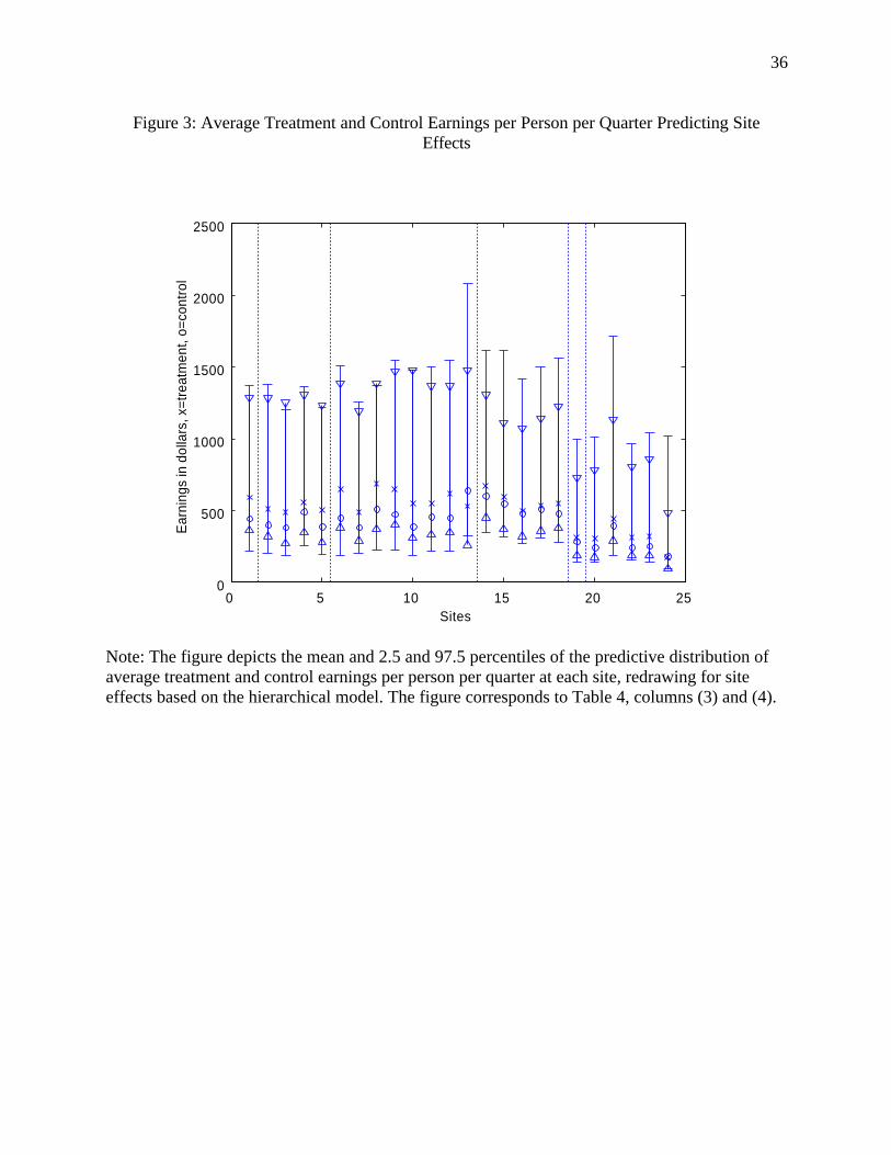
However, the range of uncertainty increases substantially (see Figures 6 and 7). In

Figure 2, the 2.5-97.5 percentile intervals of the posterior distributions overlap to a large

extent for 11 of 24 sites, and in this sense the treatment effects are not significant. In

Figure 3, the 2.5-97.5 percentile intervals for average earnings overlap for all of the 24 of

sites. In particular, for sites 2, 3, 4 and 5 (the Riverside sites), as shown in Figure 2, the

posterior 95 percent probability intervals do not overlap, but they do in Figure 3. Overall,

the comparison of the two sets of estimates suggests that when the site-specific

parameters are re-estimated for each site, we succeed in replicating a profile of outcomes

similar to those that are obtained for each site in isolation. However, uncertainty

increases, in some cases significantly.

5.4 Out-of-sample predictive uncertainty

An important question regarding site effects is whether we would be able to predict the

outcomes at a site if we had not observed that site in our data. In other words, are site

16

effects so important that it is difficult or impossible to predict the treatment effect at a

given site using data from other sites? To explore this issue, the estimates in Table 3, row

(6), drop each site successively and use the remaining sites to predict its outcome. Point

estimates of treatment effects (means of the predictive distributions) are plotted in panels

(a) and (b) of Figure 4. (The 2.5-97.5 percentile bounds are not plotted in panels (b) and

(c) because they cover almost the entire range of earnings.) The results for the two

models are broadly similar. The estimated treatment effects are within $80 on average.

Of course, some sites, for example Site 13, are off by much more. The Riverside sites are

underpredicted by $80 to $150.

One important limitation of this result is that, even though we are excluding the

site for which we are predicting the outcome, we include other sites from the same

county. Is it possible to estimate the profile of treatment effects across sites if we exclude

all of the observations from a county when estimating the model for a particular site?

The answer is presented in Table 3, row (7), and Figure 4, panel (c). For most sites the

predictions are less accurate than when other sites within the county are included. The

estimates of the treatment effect differ from the full-data estimates by an average of $150.

The Riverside sites once again are underpredicted, in this case by $114 to $170. Site 13 is

unpredicted by $307. The Los Angeles sites, which are underpredicted by an average of

$30 in panel (b), are overpredicted by an average of $157 in panel (c).

The difficulty in accurately predicting the treatment effects for these sites

illustrates the limitation of any model in extrapolating or predicting the treatment impact

at a site that is significantly different from the sites observed in the sample. Site 13 is

notably different from other sites because it has no Blacks or Hispanics; it also has the

17

lowest average level of education among participants. Likewise, the Los Angeles sites

differ from other sites in terms of the number of children, which is higher than at other

sites, and pre-treatment earnings, which are lower than at other sites. An estimator or a

functional form that is more flexible in terms of pre-treatment covariates should yield a

more reliable prediction of the treatment impact.10 In contrast, the Riverside sites do not

stand out in terms of their pre-treatment site characteristics. The differences from other

sites presumably are along qualitative dimensions of the treatment applied. The inability

to predict the Riverside treatment effects supports the view that Riverside differed from

other counties in the approach it took to administering the treatment. Predictions based on

other sites consistently under-estimate the treatment impacts in Riverside.

6. Conclusion

This paper has discussed the use of hierarchical methods to gain insight into the GAIN

data and also, more generally, to illustrate the application of these methods to datasets

which have a group or site structure.

When a dataset has a group or site structure, and when there is meaningful

heterogeneity across sites, hierarchical methods are a potentially useful tool: they allow

for a flexible modeling of site effects, for clearly distinguishing between questions of

evaluation and prediction, and for controlling the degree of smoothing (or pooling) that

the model performs with an explicitly specified parameter. The usefulness of hierarchical

methods is not confined to program evaluation. Any site or grouping structure (e.g.,

patients within a hospital, plants within a firm or under a particular manager, students

10 See for example Dehejia and Wahba (1998,1999), Heckman, Ichimura, and Todd (1997, 1998), andRosenbaum and Rubin (1983, 1985) who use propensity score methods for this purpose.

18

within a school) offers a potential application of these methods. Depending on the

application, hierarchical methods need not be estimated using Bayesian techniques. In the

present application, because the number of sites was very small, the use of the smoothing

prior was essential. In an application where the number of sites is larger, it would be

possible to allow the data to determine the degree of smoothing the model performs and

to use standard maximum likelihood methods.

Regarding the GAIN data, this paper has addressed three questions: (1) To what

extent are site effects important in evaluating a program? (2) Does predictive uncertainty

regarding site effects influence the interpretation of the treatment effect? and (3) Would

we be able to predict the outcome for a site, if its data were not observed. The answer to

the first question is that, even after accounting for differences in the composition of

program participants across sites, site-specific effects are important. Site-by-site

estimates are more variable and involve more uncertainty than pooled estimates. The

smoothed hierarchical estimate offers a compromise between these two.

The second and third questions are different because they deal with predictive

uncertainty for subsequent implementations of the program. When making in-sample

predictions, the model can predict the profile of site effects with reasonable accuracy.

This amounts to saying that even the simple set of site-level characteristics used in the

hierarchical model are sufficient to identify the distinct profile of site impacts in the

GAIN data. However, we also find that the predictive uncertainty is important in the

sense that the treatment effect for many sites ceases to be significant when predictive

uncertainty is incorporated into the estimate. Finally, when making out-of-sample

predictions, the quality of the prediction was found to depend upon observing a sufficient

19

number of sites similar to the one for which predictions are being made. For example,

when dropping even some of the Riverside sites, the quality of the predictions for all

Riverside sites declines. This is not true for the Los Angeles sites when they are dropped

singly, but becomes true when all of the observations from Los Angeles are excluded.

Was there a Riverside miracle? The received wisdom regarding the GAIN

program is that qualitative site-specific factors played an important role. The results

presented here suggest that a simple set of site characteristics are sufficient to distinguish

the various site-level effects. To this extent, there was nothing miraculous about

Riverside. However, the results also suggest that substantial extrapolation from the sites

that are observed to new sites potentially can be misleading. For example, the Riverside

treatment effects are consistently under-predicted when excluding data from all Riverside

sites. Thus, more precisely, there is nothing miraculous about Riverside if one observes

similar sites in the data. However, in the absence of data on similar sites, Riverside is

difficult to predict and to that extent is a miracle.

There are many possible extensions to this work. First, the set of site

characteristics used were rudimentary, and in principle could be extended to include

features of the local labor market or perhaps even characteristics of the program

administrators. It would be interesting to discover how much additional precision could

be obtained in that way. Second, the true economic significance of the range of

predictions from the models can be assessed only if there is an explicit decision problem.

Would the added uncertainty in predicting site-level effects be sufficient to alter the

policymaker’s decision regarding which program to choose? These are questions for on-

going research.

20

References

Albert, J. and S. Chib (1993). “Bayesian Analysis of Binary and PolychotomousResponse Data,” Journal of the American Statistical Association, 88, 669-679.

Riccio, James, Daniel Friedlander, and Stephen Freedman (1994). GAIN: Benefits,Costs, and Three-Year Impacts of a Welfare-to-Work Program. New York: ManpowerDemonstration Research Corporation.

Card, David, and Alan Krueger (1992). “Does School Quality Matter? Returns toEducation and the Characteristics of Public Schools in the United States,” Journal ofPolitical Economy, 100, 1-40.

Chamberlain, Gary, and Guido Imbens (1996). “Hierarchical Bayes Models with ManyInstrumental Variables,” Harvard Institute of Economic Research, Paper Number 1781.

Cooper, Harris, and Larry Hedges (1994), editors. The Handbook of Research Synthesis.New York: Russell Sage Foundation.

Dehejia, Rajeev (1999). “Program Evaluation as a Decision Problem,” National Bureauof Economic Research Working Paper No. 6954, forthcoming, Journal of Econometrics.

------ and Sadek Wahba (1998). “Propensity Score Matching Methods for Non-Experimental Causal Studies,” National Bureau of Economic Research Working PaperNo. 6829, forthcoming, Review of Economics and Statistics.

------ and ------ (1999). “Causal Effects in Non-Experimental Studies: Reevaluating theEvaluation of Training Programs,” Journal of the American Statistical Association,Volume 94, pp. 1053-1062.

Gelfland, A.E., and A.F.M. Smith (1990). “Sampling-Based Approaches to CalculatingMarginal Densities,” Journal of the American Statistical Association, 85, 398-409.

Gelman, Andrew, John Carlin, Hal Stern, and Donald Rubin (1996). Bayesian DataAnalysis. London: Chapman and Hall.

Geweke, John, and Michael Keane (1996). “An Empirical Analysis of the Male IncomeDynamics in the PSID: 1968-1989,” Journal of Econometrics, 96, 293-356.

Heckman, James, and Jeffrey Smith (1996). “The Sensitivity of Experimental ImpactEstimates: Evidence from the National JTPA Study,” University of Western Ontario,unpublished.

------, H. Ichimura, and P. Todd (1998). “Matching as an Econometric EvaluationEstimator: Evidence from Evaluating a Job Training Programme,” Review of EconomicStudies, 64(4) (October 1997), 605-654.

21

------, ------, and ------ (1998). “Matching as an Econometric Evaluation Estimator,”Review of Economic Studies, 65, 261-294.

Hotz, V. Joseph, Guido Imbens, and Julie Mortimer (1999). “Predicting the Efficacy ofFuture Training Programs Using Past Experiences,” National Bureau of EconomicResearch Technical Working Paper, No. 238.

------, ------, and Jacob Klerman (2000). “The Long-Term Gains from GAIN: A Re-Analysis of the Impacts of the California GAIN Program,” UCLA, unpublished.

Nelson, Doug (1997). “Some ‘Best Practices’ and ‘Most Promising Models’ for WelfareReform,” Memorandum, Annie E. Casey Foundation, Baltimore, MD;http://center.hamline.edu/mcknight/caseymemo.htm.

Rosenbaum, Paul and Donald Rubin (1983). “The Central Role of the Propensity Score inObservational Studies for Causal Effects,” Biometrika, 70, 41-55.

--------- and --------- (1985). “Constructing a Control Group Using Multivariate MatchedSampling Methods that Incorporate the Propensity Score,” American Statistician, 39, 33-38.

Rossi, Peter, Robert McCulloch, and Greg Allenby (1995). “Hierarchical Modeling ofConsumer Heterogeneity: An Application to Target Marketing,” in C. Gatsonis, J.Hodges, R. Kass, and N. Singpurwalla (eds.), Case Studies in Bayesian Statistics,Volume II, Lecture Notes in Statistics, 105. New York: Springer-Verlag.

Tanner, M., and W. Wong (1987). “The Calculation of Posterior Distributions by DataAugmentation,” Journal of the American Statistical Association, 82, 528-550.

22

Appendix: The Gibbs Sampler for the Hierarchical Model

(1) ),(~ )1()( −lj

lj VN βββ , where )ˆ'()'( 1

)1(2

)1(11

)1(2

)1(p

lljjlljjj XXXX ββσσβ −−

−−

−−−

−− Σ+Σ+= ,

jjjj yXXX ')'(ˆ 1−=β , jlp z)1(' −= γβ , and 11

)1(2

)1( ]'[ −−−

−− Σ+= lljj XXV σβ ,

(2) )(~1 212)(

2)1( sQrnl +−

+− χσ , where itjl

jitjitj xys )(][ β−= and s2=s′s,

(3) ))(,(~ 111)(

−−− ++−Σ KSMJWl ρ , where ∑ ==

J

t tt eeS1

' and tttt ze γβ −= (the Mx1vector of residuals for each site observation),

(4) ))'(,~(~ 11)(

)( −−+⊗Σ DZZN ll γγ , where )'( 1 Mγγγ L= , )(~ γγ vec= ,

)ˆ'())'(( 111 dDZZDZZ −−− ++= γγ , and jjjjj zzz βγ ')'(ˆ 1−= .

This procedure produces a sequence of draws from the parameters, the first 500 of whichwe discard, leaving us with draws from the posterior distribution of the parameters.

23

Table 1: The SampleAlameda Butte Los

AngelesRiverside San

DiegoTulare

GAIN:

Treated Group 685 1717 3730 5808 8711 2693

Control Group 682 458 2124 1706 1810 1146

Total 1367 2175 5854 7514 10521 3839

Number of Sites 1 1 5 4 8 5

Notes: The GAIN sample sizes are from the public use file of the GAIN data. TheAFDC total represents the number of AFDC cases (both single-parent and two-parenthouseholds) in the six evaluation counties in December 1990 (see Riccio, et al. (1994),Table 1.1).

24

Table 2: Site Characteristics from the GAIN ExperimentButte Riverside San Diego

Variable(samplesize)

Site 1(2165)

Site 2(3364)

Site 3(2052)

Site 4(1358)

Site 5(706)

Site 6(755)

Site 7(1457)

Site 8(1104)

Number of childrenTreatment 2.49 2.69 2.81 2.87 2.65 2.19 2.8 2.50Control 2.54 2.69 2.91 2.77 2.44 2.27 2.74 2.53(se on diff) (0.09) (0.08) (0.1) (0.13) (0.14) (0.15) (0.13) (0.13)Reading test scoreTreatment 232 231 232 231 231 230 231 231Control 227 228 227 227 226 229 229 227(se on diff) (4.56 (2.67) (4.28) (3.55) (4.89) (1.73) (2.02) (3.84)GradeTreatment 10.99 10.8 10.66 9.59 10.96 11.75 10.56 11.43Control 10.83 10.68 10.65 9.57 11.02 11.98 10.4 11.29(se on diff) (0.14) (0.1) (0.14) (0.21) (0.17) (0.24) (0.2) (0.18)Previous training experienceTreatment 0.22 0.23 0.28 0.14 0.22 0.10 0.12 0.04Control 0.24 0.24 0.25 0.14 0.22 0.09 0.11 0.06(se on diff) (0.02) (0.02) (0.02) (0.02) (0.04) (0.03) (0.02) (0.02)HispanicTreatment 0.06 0.24 0.18 0.56 0.18 0.13 0.30 0.17Control 0.07 0.24 0.2 0.58 0.19 0.17 0.32 0.14(se on diff) (0.01) (0.02) (0.02) (0.03) (0.03) (0.03) (0.03) (0.03)BlackTreatment 0.03 0.18 0.10 0.09 0.20 0.12 0.53 0.09Control 0.03 0.17 0.07 0.07 0.15 0.1 0.44 0.06(se on diff) (0.01) (0.02) (0.02) (0.02) (0.03) (0.03) (0.03) (0.02)Lagged earnings, 1 quarter before treatmentTreatment 457 388 329 478 332 487 333 514Control 432 380 359 548 381 449 447 666(se on diff) (54) (44) (53) (74) (93) (110) (59) (97)Lagged earnings, 2 quarters before treatmentTreatment 616 498 442 592 471 627 409 647Control 551 500 491 718 489 684 513 779(se on diff) (67) (51) (63) (83) (101) (131) (70) (110)Average quarterly post-treatment earningsTreatment 657 642 642 693 560 811 562 730Control 478 501 445 532 348 617 603 690(se on diff) (57) (42) (55) (66) (82) (117) (70) (94)Average quarterly treatment impact, conditional on covariatesTreatmenteffect

145 149 149 190 292 213 21 49

(se) (50) (39) (39) (56) (72) (109) (64) (90)

25

Table 2 (cont’d): Site Characteristics from the GAIN ExperimentSan Diego Tulare


Site 9(678)

Site 10(1853)

Site 11(2111)

Site 12(1897)

Site 13(630)

Site 14(500)

Site 15(531)

Site 16(1060)

Number of childrenTreatment 2.34 2.34 2.57 2.34 3.92 2.87 3.03 3.04Control 2.42 2.4 2.77 2.39 4.44 3.02 3.33 3.05(se on diff) (0.15) (0.1) (0.1) (0.09) (0.25) (0.19) (0.2) (0.14)Reading test scoreTreatment 232 231 231 231 231 230 232 231Control 227 228 229 228 228 227 226 228(se on diff) (4.63) (2.81) (2.59) (3.35) (2.61) (2.7) (5.47) (3.23)GradeTreatment 11.56 11.34 10.39 11.35 6.45 9.63 9.45 9.47Control 11.45 11.63 10.31 11.15 7.03 9.5 9.21 9.38(se on diff) (0.21) (0.15) (0.18) (0.12) (0.44) (0.32) (0.33) (0.22)Previous training experienceTreatment 0.03 0.08 0.11 0.13 0.12 0.06 0.25 0.25Control 0.04 0.11 0.1 0.16 0.12 0.08 0.22 0.2(se on diff) (0.02) (0.02) (0.02) (0.02) (0.03) (0.03) (0.04) (0.03)HispanicTreatment 0.2 0.17 0.55 0.09 0 0.62 0.43 0.34Control 0.14 0.17 0.51 0.12 0 0.63 0.49 0.29(se on diff) (0.04) (0.02) (0.03) (0.02) (0) (0.05) (0.05) (0.03)BlackTreatment 0.27 0.33 0.12 0.08 0 0.01 0 0.01Control 0.27 0.34 0.15 0.06 0 0.01 0.01 0.01(se on diff) (0.04) (0.03) (0.02) (0.02) (0.01) (0.01) (0.01) (0.01)Lagged earnings, 1 quarter before treatmentTreatment 536 456 493 498 298 476 573 439Control 470 382 531 558 234 527 366 440(se on diff) (116) (70) (70) (66) (55) (103) (103) (67)Lagged earnings, 2 quarters before treatmentTreatment 644 533 557 608 321 603 665 521Control 524 493 729 721 205 513 435 530(se on diff) (124) (81) (74) (77) (60) (104) (112) (74)Average quarterly post-treatment earningsTreatment 703 689 696 744 414 610 612 530

Control 531 496 715 676 455 641 515 444

(se on diff) (112) (72) (71) (70) (84) (96) (87) (61)

Average quarterly treatment impact, conditional on covariatesTreatmenteffect

116 195 39 104 -90 -15 25 80

(se) (104) (65) (62) (65) (77) (87) (77) (53)

26

Table 2 (cont’d): Site Characteristics from the GAIN ExperimentTulare Alameda Los Angeles


Site 17(864)

Site 18(880)

Site 19(1360)

Site 20(835)

Site 21(842)

Site 22(1485)

Site 23(1888)

Site 24(800)

Number of childrenTreatment 2.98 3.04 2.38 3.54 4.20 3.21 3.72 3.73Control 3.05 3.06 2.39 3.44 4.45 3.25 4.07 3.84(se on diff) (0.15) (0.14) (0.09) (0.16) (0.18) (0.12) (0.11) (0.17)Reading test scoreTreatment 232 231 231 232 230 230 231 231Control 226 228 228 223 228 227 229 228(se on diff) (6.29) (3.85) (3.01) (8.63) (2.32) (3.68) (1.5) (3.13)GradeTreatment 10.08 9.91 10.78 9.36 7.84 9.54 9.69 7.61Control 10.36 9.77 10.8 9.55 7.38 9.17 9.49 7.39(se on diff) (0.2) (0.26) (0.16) (0.25) (0.27) (0.2) (0.17) (0.29)Previous training experienceTreatment 0.26 0.12 0.23 0.2 0.11 0.05 0.17 0.16Control 0.19 0.11 0.25 0.14 0.12 0.05 0.15 0.17(se on diff) (0.03) (0.02) (0.02) (0.03) (0.02) (0.01) (0.02) (0.03)HispanicTreatment 0.40 0.36 0.09 0.40 0.28 0.22 0.15 0.78Control 0.38 0.38 0.06 0.30 0.24 0.18 0.16 0.73(se on diff) (0.04) (0.04) (0.01) (0.03) (0.03) (0.02) (0.02) (0.03)BlackTreatment 0.11 0.02 0.63 0.11 0.09 0.47 0.64 0.06Control 0.09 0.03 0.65 0.13 0.07 0.41 0.56 0.06(se on diff) (0.02) (0.01) (0.03) (0.02) (0.02) (0.03) (0.02) (0.02)Lagged earnings, 1 quarter before treatmentTreatment 403 544 139 136 178 175 165 62Control 597 475 145 160 199 173 146 137(se on diff) (74) (100) (33) (34) (31) (33) (30) (33)Lagged earnings, 2 quarters before treatmentTreatment 504 598 118 145 193 179 139 67Control 716 518 141 157 178 162 121 152(se on diff) (92) (104) (30) (36) (34) (32) (26) (37)Average quarterly post-treatment earningsTreatment 558 558 377 381 340 301 309 210

Control 691 691 301 301 253 311 299 269

(se on diff) (75) (75) (46) (52) (40) (43) (36) (46)

Average quarterly treatment impact, conditional on covariatesTreatmenteffect

-18 -2 84 108 80 -6 -7 -50

(se) (68) (62) (41) (49) (37) (39) (32) (44)

27Table 3: Average Earnings per Person per Quarter, Sites 1-6

Butte Riverside

Model Site 1 Site 2 Site 3 Site 4

Treated 614[601,628]

562[552,572]

535[522,548]

564[548,580](1) Pooled Control 499

[485,512]446

[436,457]422

[410,434]464

[449,479]

Treated 533[512,555]

604[587,622]

596[573,619]

672[644,702](2) Separate Control 407

[384,431]421

[403,441]366

[344,388]483

[452,515]

Treated 533[513,555]

605[586,623]

595[570,620]

672[644,703](3) Hierarchical,

no smoothing Control 407[386,430]

422[401,442]

365[344,389]

485[453,519]

Treated 590[571,609]

543[531,555]

523[510,539]


smoothed Control 436[418,456]

417[405,429]

409[395,423]

500[479,520]

Treated 401[383,418]

525[505,544]

545[524,567]

538[514,561](5)

Alamedaparticipantsin other sites Control 335

[312,356]354

[334,374]306

[284,327]333

[308,361]

Treated 589[365,1289]

510[321,1282]

489[276,1251]

553[347,1305](5)

Hierarchical,predictingsite effects Control 444

[221,1371]400

[204,1376]387

[187,1203]495

[254,1358]

Treated 609[311,2302]

502[293,2015]

477[283,2045]

537[330,2016](6)

Predictingsite effects,dropping obs.from that site

Control 458[215,3262]

397[185,2442]

390[195,2598]

501[251,2857]

Treated 609[343,1936]

479[2,7408]

456[0,7422]

536[1,7693]

(7)

Predictingsite effects,dropping obs.from thatcounty

Control 458[238,2142]

410[6,3570]

396[6,3793]

501[6,3895]

Note: The table presents the mean and 2.5 and 97.5 percentiles of the predictive distribution ofaverage earnings per person per quarter. In rows 1 to 4 and rows 5 to 7, earnings are predictedfor the original treatment and control participants at each site, under the specified models. In row4, earnings are predicted for the Alameda treatment and control participants, if they had beenlocated at the specified site.

28

Table 3 (cont’d): Average Earnings per Person per Quarter, Sites 5-8Riverside San Diego


Treated 567[547,586]

649[629,670]

535[519,550]

652[635,672](1) Pooled Control 447

[428,467]518

[498,539]424

[410,436]527

[509,543]

Treated 566[525,608]

728[683,772]

480[456,505]


[302,384]559

[499,620]440

[409,470]563

[521,605]

Treated 563[525,605]

726[684,772]

481[455,507]



558[506,611]

442[412,477]

560[511,603]

Treated 556[535,578]

623[597,650]

497[480,512]



470[444,494]

385[368,402]

544[516,570]

Treated 483[449,515]

536[508,562]

418[400,436]

494[472,518](5)


[233,293]365

[327,406]371

[344,399]435

[398,475]

Treated 507[282,1229]

644[384,1383]

485[293,1187]

689[369,1382](5)


[193,1219]451

[187,1511]386

[202,1255]514

[227,1375]

Treated 497[234,1872]

622[303,3070]

489[276,2557]

710[377,2611](6)


Control 402[176,2611]

431[140,2783]

379[168,2607]

503[174,3503]

Treated 471[1,6646]

750[4,6799]

494[3,6407]

772[9,6752]

(7)


Control 407[11,3616]

342[11,2991]

393[13,3123]

392[33,3261]

29

Table 3 (cont’d): Average Earnings per Person per Quarter, Sites 9-12San Diego


Treated 644[623,667]

599[585,613]

586[572,600]

641[625,655](1) Pooled Control 517

[497,537]475

[463,488]474

[461,486]516

[502,530]

Treated 664[619,708]

594[570,620]

561[537,582]


[500,616]467

[438,501]506

[478,537]465

[434,496]

Treated 666[622,712]

596[573,618]

562[540,586]



466[435,500]

507[475,537]

465[436,494]

Treated 641[614,667]

560[544,576]

576[561,592]



413[397,430]

486[469,504]

479[462,498]

Treated 527[499,557]

472[454,492]

479[463,496]

472[453,492](5)


[318,396]323

[299,350]416

[386,446]403

[373,432]

Treated 649[404,1471]

547[311,1474]

550[333,1366]

616[348,1367](5)


[225,1547]392

[186,1477]457

[221,1499]453

[217,1550]

Treated 645[276,2389]

542[289,2594]

545[277,2307]

624[297,2131](6)


Control 459[183,2431]

385[159,3055]

447[213,2964]

451[167,2014]

Treated 738[8,6835]

613[7,7088]

572[2,6570]

686[6,6524]

(7)


Control 355[22,2819]

354[29,3019]

369[20,3209]

376[16,2619]

30

Table 3 (cont’d): Average Earnings per Person per Quarter, Sites 13-16San Diego Tulare


Treated 410[390,428]

601[577,625]

581[556,607]

560[542,575](1) Pooled Control 344

[327,362]504

[480,527]480

[458,503]460

[445,477]

Treated 561[520,601]

620[570,668]

585[545,629]


[556,689]637

[574,701]534

[481,592]423

[393,459]

Treated 561[522,602]

614[564,666]

584[540,632]



630[564,689]

537[482,595]

423[388,456]

Treated 525[489,563]

640[606,674]

618[593,648]



538[500,576]

561[530,590]

488[465,510]

Treated 487[453,522]

445[412,480]

398[368,431]

403[377,431](5)


[664,845]439

[390,487]403

[360,449]316

[286,350]

Treated 528[263,1474]

670[452,1306]

598[374,1111]

498[325,1072](5)


[326,2082]604

[348,1613]548

[318,1615]480

[270,1416]

Treated 485[191,4007]

740[407,2786]

602[368,2141]

501[291,2531](6)


Control 886[180,8996]

592[223,3964]

555[260,2964]

505[274,3152]

Treated 476 [5,5153] 735[4,6881]

640[2,7844]

550[2,7287]

(7)


Control 839[76,3840]

598[22,4287]

578[10,4250]

534[12,4423]

31

Table 3 (cont’d): Average Earnings per Person per Quarter, Sites 17-20Tulare Alameda Los

Angeles


Treated 600[582,622]

581[561,601]

453[439,466]

401[384,418](1) Pooled Control 491

[472,510]469

[450,487]337

[326,350]297

[283,311]

Treated 510[476,542]

516[483,547]

282[259,303]


[488,571]509

[473,545]227

[209,246]251

[226,277]

Treated 513[480,548]

519[485,552]

282[262,300]



513[475,553]

226[209,243]

251[224,277]

Treated 596[576,620]

585[563,605]

343[322,364]



506[488,525]

268[251,286]

254[236,271]

Treated 361[336,385]

387[361,411]

281[260,301]

367[337,399](5)


[347,416]370

[337,404]226

[208,244]282

[256,309]

Treated 536[362,1138]

550[376,1224]

314[191,725]

303[175,779](5)


[313,1498]481

[278,1562]286

[143,991]241

[140,1011]

Treated 543[307,1983]

555[338,1987]

501[174,5522]

298[149,1834](6)


Control 511[249,2663]

478[268,2696]

717[332,4635]

238[117,2948]

Treated 595[2,7591]

589[2,7942]

314[178,879]

894[5,9228]

(7)


Control 570[7,4855]

516[15,4442]

286[132,881]

579[40,3840]

32

Table 3 (cont’d): Average Earnings per Person per Quarter, Sites 21-24Los Angeles


Treated 387[371,402]

413[401,426]

403[392,415]

307[294,323](1) Pooled Tobit Control 299

[286,314]309

[298,321]296

[286,305]223

[211,236]

Treated 427[394,460]

289[269,307]

303[286,321]

175[156,195](2) Site-by-site

Tobit Control 324[297,352]

285[263,307]

286[268,306]

200[176,224]

Treated 426[394,460]

288[268,308]

303[284,322]



286[265,307]

288[270,307]

200[178,227]

Treated 418[393,444]

325[310,339]

339[322,357]



274[260,289]

278[263,295]

198[180,217]

Treated 455[419,497]

274[257,294]

361[341,384]

267[239,296](5)


[250,316]315

[290,340]332

[310,356]275

[240,309]

Treated 447[290,1134]

312[189,805]

324[188,858]

175[96,483](5)


[188,1716]246

[152,972]257

[138,1045]184

[90,1020]

Treated 487[276,3258]

321[175,1582]

371[150,3694]

181[93,3049](6)


Control 532[271,5806]

237[119,2230]

218[107,3402]

177[71,4930]

Treated 1483[12,8219]

796[4,8013]

652[1,8072]

931[4,8998]

(7)


Control 1201[151,4040]

508[39,3050]

451[26,4224]

934[96,3974]

33

Table 4: Explanatory Power of County Dummies Conditional on Site CharacteristicsVariable Adjusted R2 of County

Dummies(0.025 and 97.5

percentiles)Constant -0.1768

[-0.2195,-0.0954]Number of Children 0.0020

[-0.1250,0.1436]Education -0.0458

[-0.1178,0.0551]Age -0.1150

[-0.2048,0.0228]1(Earningst=–2=0) -0.1322

[-0.2030,-0.0304]log(Earningst=–2+1) -0.1117

[-0.1954,0.0022]1(Earningst=–1=0) -0.1429

[-0.2028,-0.0369]log(Earningst=–1+1) -0.1177

[-0.1918,0.0120]Time trend 0.0486

[-0.0740,0.1855]Constant·Treatment -0.1086

[-0.1941,-0.0105]Number ofChildren·Treatment

-0.0800[-0.1662,0.0258]

Education·Treatment -0.0050[-0.0940,0.0983]

Age·Treatment -0.1153[-0.1903,-0.0140]

1(Earningst=–2=0)·Treatment

-0.1412[-0.2079,-0.0303]

log(Earningst=–2+1)·Treatment

-0.1161[-0.2017,0.0170]

Note: The table presents the mean and 2.5 and 97.5 percentiles of the predictive distribution ofthe adjusted R2 of a regression of site coefficients on county-level dummies.

34

Figure 1: Average Treatment Impact per Person per Quarter

0 10 20-150

-100

-50

0

50

100

150

200

250

300

Site

Trea

tmen

t Effe

ct

(a) Pooled

0 10 20-150

-100

-50

0

50

100

150

200

250

300

Site

(b) Minimum smoothing

0 10 20-150

-100

-50

0

50

100

150

200

250

300

Site

(c) Intermediate smoothing

Note: The figure depicts the mean and 2.5 and 97.5 percentiles of the predictive distribution ofthe average treatment effect per person per quarter at each site under the specified models. Panel(a) corresponds to Table 3, columns (1) and (2); Panel (b) to Table 3, columns (5) and (6); andPanel (c) to Table 3, columns (7) and (8).

35

Figure 2: Average Treatment and Control Earnings per Person per Quarter Given Site Effects

0 5 10 15 20 25100

200

300

400

500

600

700

800

Sites

Ear

ning

s in

dol

lars

, x=t

reat

men

t, o=

cont

rol

Note: The figure depicts the mean and 2.5 and 97.5 percentiles of the predictive distribution ofaverage treatment and control earnings per person per quarter at each site. The model takes theprofile of site effects as given. The figure corresponds to Table 3, columns (5) and (6).

36

Figure 3: Average Treatment and Control Earnings per Person per Quarter Predicting SiteEffects

0 5 10 15 20 250

500

1000

1500

2000

2500

Sites

Ear

ning

s in

dol

lars

, x=t

reat

men

t, o=

cont

rol

Note: The figure depicts the mean and 2.5 and 97.5 percentiles of the predictive distribution ofaverage treatment and control earnings per person per quarter at each site, redrawing for siteeffects based on the hierarchical model. The figure corresponds to Table 4, columns (3) and (4).

37

Figure 4: Average Treatment Impact per Person per Quarter

0 10 20-500

-400

-300

-200

-100

0

100

200

300

400

500

Site

Trea

tmen

t Effe

ct

(a) Full Data

0 10 20-500

-400

-300

-200

-100

0

100

200

300

400

500

Site

(b) Dropping Site

0 10 20-500

-400

-300

-200

-100

0

100

200

300

400

500

Site

(c) Dropping County

Note: The figure depicts the mean of the predictive distribution of the average treatment effectper person per quarter at each site under the specified models. Panel (a) corresponds to Table 3,columns (5) and (6); Panel (b) to Table 6, columns (1) and (2); and Panel (c) to Table 6, columns(3) and (4).

was there a riverside miracle? an hierarchical framework for

Documents