walla walla district - united states army feasibility study is to evaluate and screen structural...

F I N A L

F e b r u a r y 2 0 0 2

Lower Snake River JuvenileSalmon Migration Feasibility Report/

Environmental Impact Statement

US Army Corpsof Engineers®

Walla Walla District

APPENDIX P

Air Quality

FEASIBILITY STUDY DOCUMENTATION

Document Title Lower Snake River Juvenile Salmon Migration Feasibility Report/Environmental Impact Statement Appendix A (bound with B) Anadromous Fish Modeling Appendix B (bound with A) Resident Fish Appendix C Water Quality Appendix D Natural River Drawdown Engineering Appendix E Existing Systems and Major System Improvements Engineering Appendix F (bound with G, H) Hydrology/Hydraulics and Sedimentation Appendix G (bound with F, H) Hydroregulations Appendix H (bound with F, G) Fluvial Geomorphology Appendix I Economics Appendix J Plan Formulation Appendix K Real Estate Appendix L (bound with M) Lower Snake River Mitigation History and Status Appendix M (bound with L) Fish and Wildlife Coordination Act Report Appendix N (bound with O, P) Cultural Resources Appendix O (bound with N, P) Public Outreach Program Appendix P (bound with N, O) Air Quality Appendix Q (bound with R, T) Tribal Consultation and Coordination Appendix R (bound with Q, T) Historical Perspectives Appendix S* Snake River Maps Appendix T (bound with R, Q) Clean Water Act, Section 404(b)(1) Evaluation Appendix U Response to Public Comments *Appendix S, Lower Snake River Maps, is bound separately (out of order) to accommodate a special 11 x 17 format. The documents listed above, as well as supporting technical reports and other study information, are available on our website at http://www.nww.usace.army.mil/lsr. Copies of these documents are also available for public review at various city, county, and regional libraries.

H:\WP\1346\Appendices\FEIS\P - Air Quality\CamRdy\App_P.doc

STUDY OVERVIEW Purpose and Need

Between 1991 and 1997, due to declines in abundance, the National Marine Fisheries Service (NMFS) made the following listings of Snake River salmon or steelhead under the Endangered Species Act (ESA) as amended:

�� sockeye salmon (listed as endangered in 1991)

�� spring/summer chinook salmon (listed as threatened in 1992)

�� fall chinook salmon (listed as threatened in 1992)

�� steelhead (listed as threatened in 1997).

In 1995, NMFS issued a Biological Opinion on operations of the Federal Columbia River Power System (FCRPS). Additional opinions were issued in 1998 and 2000. The Biological Opinions established measures to halt and reverse the declines of ESA-listed species. This created the need to evaluate the feasibility, design, and engineering work for these measures.

The Corps implemented a study (after NMFS’ Biological Opinion in 1995) of alternatives associated with lower Snake River dams and reservoirs. This study was named the Lower Snake River Juvenile Salmon Migration Feasibility Study (Feasibility Study). The specific purpose and need of the Feasibility Study is to evaluate and screen structural alternatives that may increase survival of juvenile anadromous fish through the Lower Snake River Project (which includes the four lowermost dams operated by the Corps on the Snake River—Ice Harbor, Lower Monumental, Little Goose, and Lower Granite Dams) and assist in their recovery.

Development of Alternatives

The Corps’ response to the 1995 Biological Opinion and, ultimately, this Feasibility Study, evolved from a System Configuration Study (SCS) initiated in 1991. The SCS was undertaken to evaluate the technical, environmental, and economic effects of potential modifications to the configuration of Federal dams and reservoirs on the Snake and Columbia Rivers to improve survival rates for anadromous salmonids.

The SCS was conducted in two phases. Phase I was completed in June 1995. This phase was a reconnaissance-level assessment of multiple concepts including drawdown, upstream collection, additional reservoir storage, migratory canal, and other alternatives for improving conditions for anadromous salmonid migration.

The Corps completed a Phase II interim report on the Feasibility Study in December 1996. The report evaluated the feasibility of drawdown to natural river levels, spillway crest, and other improvements to existing fish passage facilities.

Based in part on a screening of actions conducted for the Phase I report and the Phase II interim report, the study now focuses on four courses of action:

�� Existing Conditions

�� Maximum Transport of Juvenile Salmon


�� Major System Improvements

�� Dam Breaching.

The results of these evaluations are presented in the combined Feasibility Report (FR) and Environmental Impact Statement (EIS). The FR/EIS provides the support for recommendations that will be made regarding decisions on future actions on the Lower Snake River Project for passage of juvenile salmonids. This appendix is a part of the FR/EIS.

Geographic Scope

The geographic area covered by the FR/EIS generally encompasses the 140-mile long lower Snake River reach between Lewiston, Idaho and the Tri-Cities in Washington. The study area does slightly vary by resource area in the FR/EIS because the affected resources have widely varying spatial characteristics throughout the lower Snake River system. For example, socioeconomic effects of a permanent drawdown could be felt throughout the whole Columbia River Basin region with the most effects taking place in the counties of southwest Washington. In contrast, effects on vegetation along the reservoirs would be confined to much smaller areas.

Identification of Alternatives

Since 1995, numerous alternatives have been identified and evaluated. Over time, the alternatives have been assigned numbers and letters that serve as unique identifiers. However, different study groups have sometimes used slightly different numbering or lettering schemes and this has led to some confusion when viewing all the work products prepared during this long period. The primary alternatives that are carried forward in the FR/EIS currently involve the following four major courses of action:

Alternative Name PATH1/

Number Corps Number

FR/EIS Number

Existing Conditions A-1 A-1 1 Maximum Transport of Juvenile Salmon A-2 A-2a 2 Major System Improvements A-2’ A-2d 3 Dam Breaching A-3 A-3a 4 1/ Plan for Analyzing and Testing Hypotheses

Summary of Alternatives

The Existing Conditions Alternative consists of continuing the fish passage facilities and project operations that were in place or under development at the time this Feasibility Study was initiated. The existing programs and plans underway would continue unless modified through future actions. Project operations include fish hatcheries and Habitat Management Units (HMUs) under the Lower Snake River Fish and Wildlife Compensation Plan (Comp Plan), recreation facilities, power generation, navigation, and irrigation. Adult and juvenile fish passage facilities would continue to operate.


The Maximum Transport of Juvenile Salmon Alternative would include all of the existing or planned structural and operational configurations from the Existing Conditions Alternative. However, this alternative assumes that the juvenile fishway systems would be operated to maximize fish transport from Lower Granite, Little Goose, and Lower Monumental and that voluntary spill would not be used to bypass fish through the spillways (except at Ice Harbor). To accommodate this maximization of transport, some measures would be taken to upgrade and improve fish handling facilities.

The Major System Improvements Alternative would provide additional improvements to what is considered under the Existing Conditions Alternative. These improvements would be focused on using surface bypass facilities such as surface bypass collectors (SBCs) and removable spillway weirs (RSWs) in conjunction with extended submerged bar screens (ESBSs) and a behavioral guidance structure (BGS). The intent of these facilities would be to provide more effective diversion of juvenile fish away from the turbines. Under this alternative, an adaptive migration strategy would allow flexibility for either in-river migration or collection and transport of juvenile fish downstream in barges and trucks.

The Dam Breaching Alternative has been referred to as the “Drawdown Alternative” in many of the study groups since late 1996 and the resulting FR/EIS reports. These two terms essentially refer to the same set of actions. Because the term drawdown can refer to many types of drawdown, the term dam breaching was created to describe the action behind the alternative. The Dam Breaching Alternative would involve significant structural modifications at the four lower Snake River dams, allowing the reservoirs to be drained and resulting in a free-flowing yet controlled river. Dam breaching would involve removing the earthen embankment sections of the four dams and then developing a channel around the powerhouses, spillways, and navigation locks. With dam breaching, the navigation locks would no longer be operational and navigation for large commercial vessels would be eliminated. Some recreation facilities would close while others would be modified and new facilities could be built in the future. The operation and maintenance of fish hatcheries and HMUs would also change, although the extent of change would probably be small and is not known at this time.

Authority

The four Corps dams of the lower Snake River were constructed and are operated and maintained under laws that may be grouped into three categories: 1) laws initially authorizing construction of the project, 2) laws specific to the project passed subsequent to construction, and 3) laws that generally apply to all Corps reservoirs.

REGIONAL BASE MAP


Corps will insert

Appendix P


Final Lower Snake River Juvenile Salmon

Migration Feasibility Report/ Environmental Impact Statement

Appendix P Air Quality

Produced by

Kennedy/Jenks Consultants

Produced for U.S. Army Corps of Engineers

Walla Walla District

February 2002

Appendix P


iii

FOREWORD Appendix P was prepared by Kennedy/Jenks Consultants in conjunction with the U.S. Army Corps of Engineers’ (Corps) study team. Foster Wheeler Environmental Corporation also contributed to this appendix. In addition, the air quality analysis required extensive input from the Transportation and Power studies by the Drawdown Regional Economic Workgroup (DREW) that were undertaken as part of Appendix I, Economics. This appendix is one part of the overall effort of the Corps to prepare the Lower Snake River Juvenile Salmon Migration Feasibility Report/Environmental Impact Statement (FR/EIS).

The Corps has reached out to regional stakeholders (Federal agencies, tribes, states, local governmental entities, organizations, and individuals) during the development of the FR/EIS and appendices. This effort resulted in many of these regional stakeholders providing input and comments, and even drafting work products or portions of these documents. This regional input provided the Corps with an insight and perspective not found in previous processes. A great deal of this information was subsequently included in the FR/EIS and appendices; therefore, not all of the opinions and/or findings herein may reflect the official policy or position of the Corps.

Appendix P

TABLE OF CONTENTS


v

Executive Summary P ES-1

1. Introduction: Scope and Issues Development P1-1 1.1 Issues Raised During the Scoping Process P1-2 1.2 The Study Process P1-3

2. Air Quality of the Lower Snake River P2-1 2.1 Air Quality Management P2-1 2.2 Overview of Existing Air Quality P2-7 2.3 Existing Air Quality P2-13 2.4 Climatic Factors P2-17

3. Study Methods P3-1 3.1 Demolition Fugitive Emissions P3-1 3.2 Loss of Barge Traffic P3-8 3.3 Windblown Fugitive Dust P3-15 3.4 Replacement Power Generation P3-22

4. The Alternatives and Their Impacts P4-1 4.1 Existing Conditions Alternative P4-1 4.2 Major System Improvements Alternative P4-7 4.3 Dam Breaching Alternative P4-9

5. Comparison of Alternatives P5-1 5.1 Summary of Emissions by Alternative P5-1 5.2 Existing Conditions Alternative P5-1 5.3 Major System Improvements Alternative P5-4 5.4 Dam Breaching Alternative P5-5

6. Literature Cited P6-1

7. Glossary P7-1 Annex A Supplemental Climatology Data Annex B Highway Wheat and Barley Flows With and Without the Snake River Waterway Annex C Predicted PM10 Concentrations for Storm Events Annex D Population Distribution Map

Appendix P

FIGURES


vi

Figure 2-1. Atmospheric Emissions for Counties Adjacent to the Lower Snake River P2-11 Figure 2-2. Atmospheric Emissions by Source Category for Counties Adjacent to the Lower

Snake River P2-12 Figure 2-3. Regional Precipitation P2-20 Figure 2-4. Average Monthly Precipitation Totals P2-21 Figure 2-5. Average Monthly Temperatures P2-22 Figure 2-6. Ice Harbor, Washington Windrose for August 1999�October 2000 P2-24 Figure 2-7. Pendleton, Oregon Windrose for 1984�1991 P2-25 Figure 2-8. Spokane, Washington Windrose for 1984�1991 P2-26 Figure 2-9. Yakima, Washington Windrose for 1984�1991 P2-27 Figure 3-1. The Relationship Between Peak Gusts and One-Hour Average Wind Speeds P3-19 Figure 3-2. Average Number of Hours Per Year of High Wind Speed Events P3-19 Figure 3-3. PM10 Emission Factors by 1-Hour Average Wind Speed P3-20 Figure 4-1. Predicted 24-Hour PM10 Concentrations from Excavations at Lower Monumental

Dam P4-13 Figure 4-2. Predicted 24-Hour PM10 Concentrations from Quarry Operations P4-14 Figure 4-3. Predicted 24-Hour PM10 Concentrations with Distance South of the Ice Harbor

Dam P4-15 Figure 4-4. Frequency of Occurrence of Predicted Emissions for Individual Wind Events P4-23

Appendix P

TABLES


vii

Table 2-1. Ambient Air Quality Standards P2-2 Table 2-2. Historical Carbon Dioxide Emissions P2-8 Table 2-3. Major Air Emission Sources within the Region of the Lower Snake River P2-10 Table 2-4. Regional Ambient Air Pollutant Concentrations P2-13 Table 2-5. Peak 24-hour Concentrations and the Expected Number of Exceedances Per Year

near Owens Lake, California P2-16 Table 2-6. Effectiveness of Owens Lake Fugitive Dust Emission Control Strategies P2-16 Table 2-7. Wind Directions and Speeds for Selected Monitoring Stations P2-23 Table 3-1. Fugitive Dust Emission Equations P3-2 Table 3-2. Default Values for Emission Calculations P3-3 Table 3-3. Excavation Quantities P3-4 Table 3-4. Deconstruction Engineering Data P3-4 Table 3-5. Quarry Excavation Quantities P3-6 Table 3-6. Mobile Source Emission Factors P3-10 Table 3-7. Energy Requirements by Transportation Mode P3-10 Table 3-8. Ton-miles for the 1994 Wheat and Barley Harvest with Snake River Barge

Transportation P3-10 Table 3-9. Ton-miles for the 1994 Wheat and Barley Harvest without the Snake River Barge

Transportation P3-11 Table 3-10. Change in Transportation Bushel-Miles Resulting from Drawdown P3-12 Table 3-11. Traffic Counts P3-13 Table 3-12. Highway Emissions Used in Modeling P3-15 Table 3-13. Area of Lower Snake River Reservoirs P3-21 Table 3-14. Average Uncontrolled Combustion Emission Factors P3-24 Table 4-1. Lower Snake River Commodity Tonnage for 1994 P4-2 Table 4-2. Unadjusted Wheat and Barley Transportation-Related Emissions for Snake River

Towboats P4-3 Table 4-3. Unadjusted Towboat Emissions for Alternative 1—Existing Conditions P4-4 Table 4-4. Predicted Concentrations Resulting from Towboat Emissions P4-5 Table 4-5. Towboat Concentrations as a Percent of the Ambient Air Quality Standards P4-5 Table 4-6. Predicted Highway Concentrations P4-6 Table 4-7. Measured PM10 Concentrations during Eastern Washington Storm Events P4-7 Table 4-8. Power Generating Emissions for Existing Conditions Alternative P4-8 Table 4-9. Estimated Deconstruction PM10 Emissions P4-11 Table 4-10. Estimated Emissions from Quarry Activities P4-11 Table 4-11. Unadjusted Wheat and Barley Transportation-Related Emissions without the

Snake River Barge Transportation P4-17 Table 4-12. Change in Transportation-Related Emissions Following Dam Breaching P4-18 Table 4-13. Change in the Number of Trucks Following Dam Breaching P4-19

Appendix P

TABLES


viii

Table 4-14. Predicted Highway Concentrations Following Drawdown P4-20 Table 4-15. Annual Estimated Windblown PM10 Emissions P4-22 Table 4-16. Hazardous Air Pollutant Concentrations P4-26 Table 4-17. Summary of Recent Power Plants Constructed or to Be Constructed in the Pacific

Northwest P4-28 Table 4-18. Summary of Air Quality Impacts from a 248 MW Power Station P4-29 Table 4-19. Summary of Air Quality Impacts from a 660 MW Power Station P4-30 Table 4-20. Percent Increase in Year 2010 Electrical Generating Emissions Throughout

WSCC Region P4-31 Table 4-21. Year 2010 WSCC Regional Emissions for New Power Plants Scenario P4-33 Table 4-22. Achievable Conservation for Zero Carbon Scenario P4-34 Table 5-1. Summary of Emissions in Tons P5-2 Table 5-2. Summary of Maximum Predicted Ambient Air Concentrations P5-3

Appendix P

ACRONYMS AND ABBREVIATIONS


ix

�C degrees Celsius �F degrees Fahrenheit �g/m3 micrograms per cubic meter AAQS ambient air quality standards aMW average megawatt ASIL Acceptable Source Impact Level BACT best available control technology BGS Behavioral Guidance System BPA Bonneville Power Administration Btu British thermal unit CAM compliance assurance monitoring CCAP U.S. Climate Change Action Plan CEMS continuous emission monitoring system CFC chlorofluorocarbons CFR Code of Federal Regulations CH4 methane cm centimeter CO carbon monoxide CO2 carbon dioxide Comp Plan Lower Snake River Fish and Wildlife Compensation Plan Corps U.S. Army Corps of Engineers CP3 Columbia Plateau PM10 Program DDT 1,1,1-trichloro-2,2-bis(p-chlorophenyl)-ethane DREW Drawdown Regional Economic Workgroup EC energy consumption Ecology Washington State Department of Ecology EF emission factor EFSEC Washington State Energy Facility Siting Evaluation Council EIS environmental impact statement EPA U.S. Environmental Protection Agency ESA Endangered Species Act ESBS extended submersible bar screen EWITS Eastern Washington Intermodal Transportation Study FCAA Federal Clean Air Act FCCC Framework Convention on Climate Change Feasibility Study Lower Snake River Juvenile Salmon Migration Feasibility Study FR/EIS Lower Snake River Juvenile Salmon Feasibility Report/ Environmental Impact Statement g gram gal gallon GAMS General Algebraic Modeling System GHG greenhouse gas GIS geographic information system g/sec-m2

grams per second per square meter

Appendix P



x

HAP hazardous air pollutant HCFC partially halogenated fluorocarbons HMU Habitat Management Unit hp horsepower HRSG heat recovery steam generator IPCC Intergovernmental Panel on Climate Change IPP independent power producer ISC Industrial Source Complex k dimensionless aerodynamic particle size multiplier kg kilogram kg/hour kilograms per hour km kilometer km/hour kilometers per hour LAER lowest achievable emission rate lb pound lb/gal pounds per gallon m meter M moisture content m/s meters per second m2 square meter m3 cubic meter mm millimeter mph miles per hour MT metric ton (1,000 kg) MTY metric tons per year MW megawatt N2O nitrous oxide NCDC National Climatic Data Center NESHAP National Emission Standards for Hazardous Air Pollutants NH3 ammonia NMFS National Marine Fisheries Service NO2 nitrogen dioxide NOAA National Oceanic and Atmospheric Administration NOC Notice of Construction NROC Natural Resources Defense Council NWPPC Northwest Power Planning Council NOx nitrogen oxides NSR New Source Review O3 ozone ODEQ Oregon Department of Environmental Quality p number of days per year with measurable precipitation Pb lead PG&E Pacific Gas and Electric Company PM particulate matter

Appendix P



xi

PM10 particulate matter with aerodynamic diameters less than 10 micrometers PM2.5 particulate matter with aerodynamic diameters less than 2.5 micrometers ppm parts per million ppmv parts per million by volume PROSYM power system model PSD prevention of significant deterioration RM River Mile S mean vehicle speed s silt content SBC surface bypass collector SCE Southern California Edison SCR selective catalytic reduction SDG&E San Diego Gas and Electric SEPA Washington State Environmental Policy Act SIP Washington State Implementation Plan SO2 sulfur dioxide SOR system operation review SR state route TAP toxic air pollutant TPY tons per year TSP total suspended particulates u mean wind speed ufm fastest mile ufv frictional velocity utv threshold frictional velocity VKT vehicle kilometers traveled VM vehicle miles VMT vehicle miles traveled VOC volatile organic compound W mean vehicle weight WAC Washington Administrative Code WEAQP Wind Erosion Air Quality Project WSCC Western Systems Coordinating Council WSDOT Washington State Department of Transportation yd yard yd3 cubic yard

Appendix P


xii

ENGLISH TO METRIC CONVERSION FACTORS

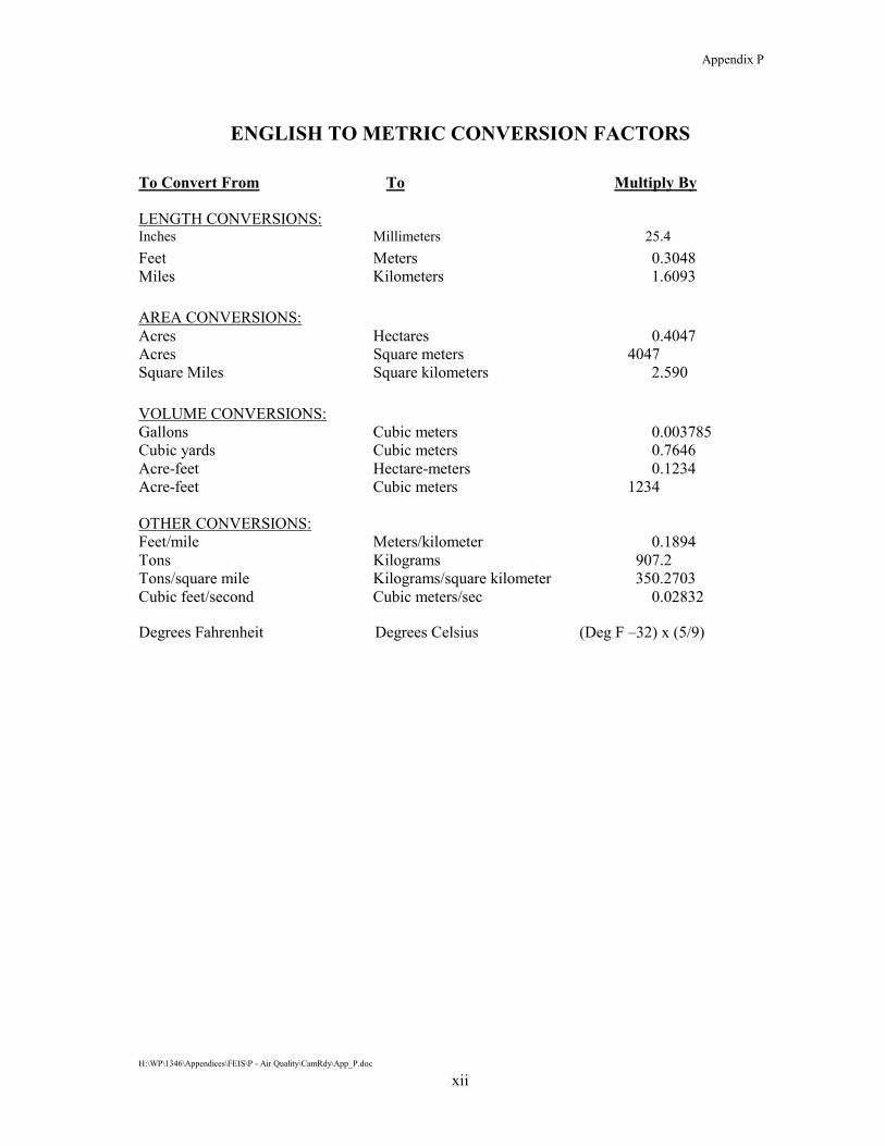
To Convert From To Multiply By LENGTH CONVERSIONS: Inches Millimeters 25.4 Feet Meters 0.3048 Miles Kilometers 1.6093 AREA CONVERSIONS: Acres Hectares 0.4047 Acres Square meters 4047 Square Miles Square kilometers 2.590 VOLUME CONVERSIONS: Gallons Cubic meters 0.003785 Cubic yards Cubic meters 0.7646 Acre-feet Hectare-meters 0.1234 Acre-feet Cubic meters 1234 OTHER CONVERSIONS: Feet/mile Meters/kilometer 0.1894 Tons Kilograms 907.2 Tons/square mile Kilograms/square kilometer 350.2703 Cubic feet/second Cubic meters/sec 0.02832

Degrees Fahrenheit Degrees Celsius (Deg F –32) x (5/9)

Appendix P


P ES-1

Executive Summary In response to the National Marine Fisheries Service 1995 Biological Opinion concerning the operation of the Federal Columbia River Power System, the U.S. Army Corps of Engineers is studying structural and operational alternatives to improve the downstream migration of juvenile salmon through the lower Snake River dams. The four alternatives that the U.S. Army Corps of Engineers is considering are:

�� Alternative 1—Existing Conditions

�� Alternative 2—Maximum Transport of Juvenile Fish

�� Alternative 3—Major System Improvements

�� Alternative 4—Dam Breaching.

From an air quality perspective, there is no difference in the impacts of the second and third alternatives. Accordingly, these two alternatives have been combined, and the following three air quality alternatives are evaluated:

�� Existing Conditions�corresponding to Lower Snake River Juvenile Salmon Migration Feasibility Report/Environmental Impact Statement (FR/EIS) Alternative 1

�� Major System Improvements�corresponding to FR/EIS Alternatives 2 and 3

�� Dam Breaching�corresponding to FR/EIS Alternative 4.

Implementation of any of the proposed alternatives would affect air quality in the lower Snake River area. The information in this appendix may be used to compare the Lower Snake River Juvenile Salmon Migration FR/EIS alternatives from an air quality perspective and may be used with other investigations to develop a comprehensive picture of the consequences of the alternatives.

The Existing Conditions alternative represents current conditions during a base line year (generally 2010). The Major System Improvements alternative represents the base line year following structural enhancements to improve fish migration. The greatest change in emissions would be associated with the Dam Breaching alternative. Air quality issues associated with the Dam Breaching alternative include the following:

�� Fugitive dust emissions generated during deconstruction of the dams

�� A change in the quantity and distribution of vehicle emissions as Snake River commerce shifts from barges to trains and trucks

�� Fugitive emissions resulting from dry exposed lake sediments during storm-generated high wind speeds

�� Atmospheric emissions from new thermal power plants built to replace lost hydropower generating capacity.

Air quality issues associated with this alternative define the areas to be investigated. These same areas are investigated for the other alternatives to define base line conditions. The technical sections

Appendix P


P ES-2

of this appendix present and summarize each of these four issues by alternative. The summary below describes these emissions issues, organized by alternative.

Construction and Deconstruction Fugitive Dust

The Existing Conditions alternative would not result in demolition of the lower Snake River dams. Therefore, there would not be any fugitive dust emissions from deconstruction. Although the dams would remain intact for the Major System Improvements alternative, there would be some construction activities. Construction-related emissions would be very small and would be limited to particulate matter, which has been conservatively estimated at 907.2 kilograms (kg) per year (1 ton per year [TPY]). Construction equipment tailpipe emissions were not estimated.

The Dam Breaching alternative would result in deconstruction of the four lower Snake River dams. Deconstruction-related emissions for this alternative include fugitive emissions from material handling activities such as hauling, dumping, bulldozing, and grading. The emission estimates for particulate matter with aerodynamic diameters of less than 10 micrometers (PM10) were derived from EPA emission factors, equipment operating hours, and the volume of material to be excavated. They account for construction mitigation measures such as spraying haul roads with water. The PM10 emissions of 1,193 tons were estimated by assuming that demolition of all four dams would take place in 1 year. This is a conservative assumption. The Drawdown Engineering Appendix (Appendix D) calls for a 2-year deconstruction schedule. Construction vehicle tailpipe emissions were not estimated.

The air quality analysis predicted ambient PM10 concentrations resulting from haul road fugitive dust emissions. The Lower Monumental stockpile haul road and the haul road for one of the three quarries were modeled using worst-case meteorology and EPA dispersion models. The proposed Lower Monumental excavation schedule is very short, resulting in the largest haul road emissions. Predicted PM10 concentrations are less than the Ambient Air Quality Standards (AAQS) within a short distance from the haul road. The area of restricted public access will be defined before deconstruction begins. Deconstruction emissions were also modeled to determine impacts in the Wallula nonattainment area, located about 18 kilometers (km) (11 miles) south-southwest of Ice Harbor. Predicted 24-hour PM10 concentrations were less than the 5 micrograms per cubic meter (µg/m3) significance level. Emissions from dam deconstruction would not be allowed to delay the date for obtaining attainment status in the Wallala nonattainment area or to contribute to an air quality standard violation (WAC 173-400-113). This requirement is satisfied if the predicted concentrations are less than the significance levels. Nonattainment area concentrations greater than the significance levels require the source to offset its emissions.

Transportation Emissions

In 1994, more than 3.8 million metric tons (4.2 million tons) of freight passed through the Ice Harbor locks. About 80 percent of the river commerce is the downriver transportation of farm products, particularly grain. The Dam Breaching alternative would shift this commerce from barges to trains and trucks. Locomotive and truck emissions would replace Snake River towboat emissions.

Transportation-related emissions were estimated by modeling the movement of grain from farms through intermediate elevators to barges, trains, and trucks. EPA emission factors were used to convert bushel-miles or ton-miles predicted by the models to tons of emitted pollutants. The emission estimates were increased to account for all commodities (not just grain), increases in

Appendix P


P ES-3

commerce by 2010, and the return of empty containers. Transportation-related emissions for the Existing Conditions and Major System Improvements alternatives would represent base-case emissions for 2010. Dam Breaching alternative emissions are for 2010 without the Snake River waterway. The estimated emissions and the change in emissions are as follows:

Emissions (tons) Pollutant CO NOx PM10 SO2 VOC Existing Conditions 235 1,705 52 266 285 Major System Improvements 235 1,705 52 266 285 Percent Change from Existing Conditions 0 0 0 0 0 Dam Breaching 227 1,759 63 198 383 Percent Change from Existing Conditions (3) 3 21 (26) 11 CO=carbon monxide, NOx=nitrogen oxides, PM10=particulate matter with aerodynamic diameters less than 10 micrometers, SO2=sulfur dioxide, VOC=volatile organic compound.

Grain shipped on the Snake River is first trucked to elevators at river ports. Without the Snake river waterway, the grain would be trucked to elevators located next to railroads or to other ports on the Columbia River. Without the waterway, truck traffic would become concentrated on roads that lead to and from the Tri-Cities, especially U.S. 395. Local and rural roads east of Pasco would also receive much of the increased truck traffic. The modeled number of bushels of grain on eastern Washington roads, with and without the Snake River waterway, may be used to estimate the change in the number of trucks on major eastern Washington highways. The total number of trucks required for the grain harvest and the average number of trucks per day, at selected intersections, are as follows:

Total Number of Trucks1/ Number of Trucks Per Day

Highway Intersection With Snake River Dams

Without Snake River Dams Current

Change with

Drawdown Projected Percent Change

US 395 SR 26 6,923 68,083 2,480 1,003 3,483 40 SR 260 6,923 68,198 2,160 1,005 3,165 47 SR 127 SR 26 6,923 3,462 290 (57) 233 (20) SR 195 SR 272 21,923 8,077 1,920 (227) 1,693 (12) SR 26 SR 395 6,923 31,385 375 401 776 107 SR 195 3,462 21,923 575 303 878 53 SR 260 West of 395 6,923 2,308 884 (76) 808 (9) East of 395 3,462 2,308 195 (19) 176 (10) SR=State Route. 1/ Total number of trucks per grain-harvesting season.

The greatest increase in truck traffic would take place along roads that are already heavily traveled. Traffic along highways used to haul grain to river ports would decrease. Truck traffic on some little-used roads may double.

All transportation-related emissions would continue to decline in the future as fuel efficiencies improve and national emissions standards become effective. Emissions standards for locomotives took effect in 2000. Emissions standards for compression-ignition marine engines are proposed to become effective in 2004. The first phase of a proposed strategy to reduce emissions from heavy-duty vehicles would become effective in 2004.

Appendix P


P ES-4

Vehicle emissions were modeled to determine transportation-related impacts. Towboat emissions for barges navigating the Snake River and moored at hard rock dolphins combined to produce ambient concentrations that are a small fraction of the AAQS. Vehicle traffic at the intersection of US 395 and State Route (SR) 260 was modeled to estimate the impacts associated with additional grain trucks following dam breaching. The impacts were maximized by assuming that grain shipments continue all year. The predicted concentrations increased by only several percent. The annual nitrogen oxides (NOx) concentrations increased from 25 to 27 percent of the ambient air quality standard.

Windblown Fugitive Dust

Windblown dust would continue to be the major air quality problem in eastern Washington. Dust storms would continue to occur periodically in the region. Under the Existing Conditions and Major System Improvements alternatives, the dust sources would be rangeland, irrigated agricultural lands, and dry agricultural lands, including fallow lands and harvested lands with crop residue. The period when these lands are most susceptible to erosion is September through November, after harvesting is completed and before winter rains begin. During this period, about 10 storms per year can be expected to produce fugitive emissions of varying intensity.

The Columbia Plateau PM10 Program (CP3) has studied windblown dust and agricultural practices that would reduce emissions. Four of the larger storms from 1990 through 1993 were modeled by CP3 to estimate emissions during these events and the resulting fugitive dust concentrations. Particulate matter emitted from between 0.809 and 2.023 million hectares (2 and 5 million acres) ranged from 10,900 to 213,200 metric tons (12,000 to 235,000 tons) per event. Daily PM10 concentrations measured in the Kennewick and Spokane areas were between 126 and 1,166 �g/m3 (the air quality standard is 150 �g/m3). PM10 concentrations in the area of the Ice Harbor and Lower Monumental dams were predicted to be about 2,400 �g/m3 during these storms.

The Dam Breaching alternative would eliminate the lower Snake River reservoirs, creating large areas of dry lake sediments. Until seeding could establish a vegetative cover, these sediments would be susceptible to wind erosion. If strong winds such as those modeled by CP3 occurred when the dry reservoir sediments were unprotected, PM10 emissions of between 354 and 3,520 metric tons (390 and 3,880 tons) per storm could be expected. These emissions would be 0.4 to 13 percent of the total emissions from agricultural lands.

Many individual storms would produce less than 181 metric tons (200 tons) of PM10 from all four dry reservoirs. All four dry reservoirs exposed for 1 year would emit about 5,706 metric tons (6,290 tons) of PM10. These estimates include mitigation through seeding. Tests at Owens Lake in California indicate that a 99 percent emissions reduction is possible by covering only 50 percent of the dry sediments with vegetation. Three phases of drill seeding would follow the initial application of seed and fertilizer by aerial methods. The Corps would take measures to prohibit recreational vehicles on the dry sediments from breaking the surface crust and causing more material to be susceptible to erosion. The emission estimates include a 90 percent reduction factor for mitigation.

The CP3 modeled PM10 emitted during several eastern Washington dust storms and calibrated the results with measured concentrations. This effort indicated that 24-hour concentrations in the region between Kennewick and Spokane can be much more than 150 µg/m3, the AAQS. Land use and soil type data used in the modeling were recently modified to simulate the dry Snake River reservoirs. One storm event previously analyzed was remodeled. This analysis indicates that although the dry

Appendix P


P ES-5

reservoirs will be subject to wind erosion, the additional concentrations resulting from lake sediments will be much less than the AAQS. PM10 concentrations in eastern Washington will continue to exceed the AAQS. It is possible that portions of eastern Washington may be reclassified as nonattainment. If areas adjacent to the reservoirs are reclassified as nonattainment, impacts associated with wind blown dust from dry sediments could be significant and will need to be reevaluated.

Water quality studies (Appendix C) indicated that some sediments contain contaminants, particularly metals, dioxin, and DDT. Fugitive dust originating from these sediments will contain the contaminants. Exposure to contaminants at concentrations equal to their Acceptable Source Impact Level (ASIL), established by the Washington State Department of Ecology, will result in health risks of less than 1 in 1,000,000. The measured sediment contaminant concentrations would result in ambient concentrations less than ASILs, assuming that the contaminant concentrations in all exposed sediments are equal to the maximum measured concentration.

Replacement Power Emissions

Demand for power will continue to increase in the future regardless of actions taken at the Snake River dams, requiring additional generating capacity. Under the Existing Conditions and Major System Improvements alternatives, hydropower would continue to be available from the lower Snake River Dams. Under the Dam Breaching alternative, hydropower would no longer be available from the lower Snake River dams. The loss of these dams would affect the generating resources of the Western System Coordinating Council (WSCC), which includes the roughly 2,000 existing electrical generating units in the western United States. The Technical Report on Hydropower Costs and Benefits evaluated the need for additional generating capacity throughout the WSCC. Annual emissions from approximately 2,000 generating units were estimated from the number of hours each unit was projected to operate. The emission estimates represent the year 2010 and include additional natural-gas-fired, combined-cycle power plants. Carbon dioxide (CO2), carbon monoxide (CO), PM10, volatile organic compounds (VOCs), benzene, and formaldehyde emissions were estimated from the projected emissions and EPA emission factors for various fuels.

The Dam Breaching alternative includes two sub-alternatives. Under the New Power Plants scenario, new fossil-fuel power plants would replace all of the hydropower lost from the Lower Snake River dams. Under the Zero Carbon scenario, the lost hydropower would be replaced by implementing regional energy conservation measures and constructing new power plants that use nonpolluting renewable energy. The Hydropower Costs and Benefits Report evaluated costs associated with replacing power generated by the lower Snake River dams and concluded that it is not necessary to replace all 3,500 MW of peak generating capacity because the actual average annual power output from the dams is about 1,200 MW. The most likely scenario with dam breaching is construction of 1,550 MW of generating capacity somewhere in the Pacific Northwest by 2010.

The thermal power plants recently added to the WSCC have been predominantly natural-gas-fired, combined-cycle plants with combustion turbines. Nine of these plants have been constructed in Oregon and Washington since 1991, and another seven are planned. Because of their low cost, abundance of suitable sites, and favorable technical characteristics, natural-gas-fired, combined-cycle plants are the most likely power plants to be built in the near future (based on the year 2000 energy market). The hydropower study team concluded that for the New Power Plants

Appendix P


P ES-6

scenario, six new combined-cycle power plants (each with a 250 MW peak capacity) would be constructed in Washington or Oregon as replacement power under dam breaching.

Replacement power plants would likely share many of the characteristics of recently constructed and planned power plants. The emission characteristics for the replacement power plants were evaluated by inspecting the air quality permits for two actual power plants that have recently been permitted in Washington: a 248 MW plant near Vancouver and a 660 MW plant near Bellingham. New power plants would be subject to state and local air quality permitting and must demonstrate the use of best available control technology (BACT). Turbine emissions would be controlled by several technologies. NOx control is obtained by using low NOx burners and selective catalytic reduction (SCR). CO, VOC, and hazardous air pollutants are controlled by good combustion and a catalytic oxidation system. PM10 and sulfur dioxide (SO2) emissions are controlled by using clean fuels such as natural gas and limiting the amount of fuel oil that can be used as backup fuel each year. This combination of emission controls satisfies BACT, and would also satisfy the National Emission Standards for Hazardous Air Pollutants (NESHAP), which EPA will soon propose for combustion turbines. Average annual emissions from the representative power plants would be as follows:

Annual Emissions from Each 250 MW Combined-Cycle Power Plant CO NOx PM10 SO2 VOC Ammonia Formaldehyde Emissions (tons/year) 88 99 41 48 30 93 0.5 Local ambient air pollutant concentrations within a few miles of each power plant were evaluated based on inspecting the air quality permits for the two representative actual power plants. The concentrations for all pollutants from the two actual power plants were all lower than the national, state, and local ambient air quality limits.

Total regional emissions for the Existing Conditions alternative and the Dam Breaching alternative were estimated for all of the roughly 2,000 generating units in the WSCC. Estimated emissions for each alternative and the change in emissions with the two Dam Breaching scenarios are as follows:

Year 2010 Emissions in WSCC (thousands of tons per year) CO CO2 NOx PM10 SO2 VOC Benzene FormaldehydeAlternative Existing Conditions 404 414,234 57.8 49 457 1 0.004 0.04 Major System Improvements 404 414,234 57.8 49 457 1 0.004 0.04 New Power Plants 408 418,870 58.1 49 459 1 0.004 0.04 Zero Carbon 404 414,234 57.8 49 457 1 0.004 0.04 Increase for New Power Plants (%)

1.0 1.1 0.5 0.4 0.4 0.2 0.4 0.005

Increase for Zero Carbon (%) 0 0 0 0 0 0 0 0

Nationwide and regional CO2 emissions are important because of possible impacts to global warming. In the 8-year period from 1990 to 1998, U.S. CO2 emissions increased by about 11 percent, from 9,806 million to 10,932 million metric tons (10,809 to 12,050 million tons). If greenhouse gas emissions continue to increase at this rate, nationwide CO2 emissions will reach 12,519 million metric tons (13,800 million tons) by 2010. The replacement power plants for the New Power Plants scenario could increase regional CO2 emissions by 4.6 million tons per year. That increase would be equivalent to 1.1 percent of the total CO2 emissions within the WSCC and

Appendix P


P ES-7

would be 0.14 percent of the nationwide CO2 emission increase during the planning period 1990-2010.

Under the Zero Carbon scenario, the hydropower lost from the Lower Snake River dams would be replaced by conservation measures and development of nonpolluting renewable energy resources. The required energy conservation measures would be equivalent to 5.3 percent of the total electrical demand in the WSCC region for the year 2010. There would be no net increase in CO2 emissions under the Zero Carbon scenario.

Appendix P


P1-1

1. Introduction: Scope and Issues Development

The Lower Snake River Juvenile Salmon Migration Feasibility Study (Feasibility Study) assessed the measures intended to facilitate migration of juvenile salmon through the lower Snake River. Implementation of the proposed measures would result in air quality-related effects. The purpose of this air quality appendix is to estimate changes in air pollutant concentrations associated with the Feasibility Study alternatives and to qualitatively evaluate indirect impacts associated with dam breaching. In several instances, emission sources are located in airsheds other than along the lower Snake River.

To evaluate air quality impacts, the alternatives considered in the Lower Snake River Juvenile Salmon Migration Feasibility Report/Environmental Impact Statement (FR/EIS) were used to create alternatives for the air quality investigation. Although the FR/EIS identifies four alternatives, the air quality impacts of FR/EIS Alternatives 2 and 3 are almost identical. The evaluations of Alternatives 2 and 3 are therefore combined in this appendix, yielding the following three air quality investigation alternatives:

�� Existing Conditions (FR/EIS Alternative 1)�The status of the lower Snake River reservoirs and hydrofacilities would remain unchanged. Emissions estimated for this alternative represent current conditions for a base line year.

�� Major System Improvements (FR/EIS Alternatives 2 and 3)�Collection and bypass structures would be constructed at all hydropower facilities to enhance fish passage. Barge transportation and power generation would continue with little change.

�� Dam Breaching (FR/EIS Alternative 4)�The four lower Snake River hydropower facilities would be breached, restoring the river to near-natural conditions. Barge transportation and hydropower would be replaced with other sources of transportation and power generation.

�� The air quality issues related to the Lower Snake River Juvenile Salmon Migration Feasibility Study alternatives are:

�� Fugitive dust emissions resulting from deconstruction of the dams

�� Changes in the quantity and distribution of vehicle emissions as commodities are shifted from barges to trains and trucks

�� Fugitive dust emissions resulting from dry exposed lake sediments during high wind speed events

�� Atmospheric emissions associated with replacement power generation by thermal power plants.

Cumulative impacts evaluated in this analysis include the effects of breaching all four dams in one year and building all replacement power plants at once. Some impacts associated with indirect effects are subject to socioeconomic conditions and factors that are beyond the scope of this assessment. This appendix contains seven sections. Section 1 summarizes the air quality issues

Appendix P


P1-2

associated with the Feasibility Study and provides an overview of the study process. Section 2 describes the air quality of the lower Snake River area, including the Federal and state programs that regulate air quality in the region of the lower Snake River and the air quality standards relevant to the analysis. The climatology and existing air quality of the region are also described. Section 3 presents the methods that this study uses for the air quality analysis. Section 4 presents the study results for the Feasibility Study alternatives and potential mitigation measures. Section 5 compares the air quality impacts of the alternatives. Sections 6 and 7 contain the references and glossary, respectively. Technical annexes A through D support the analysis and are included.

1.1 Issues Raised During the Scoping Process The multi-agency System Operation Review (SOR) of the Columbia and Snake rivers included an analysis of the consequences to air quality resulting from the annual or permanent drawdown of reservoirs (Bonneville Power Administration [BPA], U.S. Army Corps of Engineers [Corps], and Bureau of Reclamation, 1995, SOR Appendix B). This analysis builds on the SOR work while focusing on the four lower Snake River dams. Some of the air quality issues identified during the SOR have been carried over to this study.

A number of additional air quality issues related to the Dam Breaching alternative have been identified, including the following:

�� Cumulative impacts of new and existing power plants

�� Greenhouse gases (GHG) and hazardous air pollutants (HAP) from replacement power generation

�� Site-specific data for characterizing air quality impacts

�� Mobile source emission impacts on existing highways and roadways

�� Cumulative impacts of demolishing more than one dam at a time

�� Contaminants potentially present in reservoir sediments that may become airborne during dust storms.

The objective of this appendix is to provide a basis to compare impacts of the Feasibility Study pathways from an air quality perspective. This is accomplished by estimating air emissions resulting from pathway-related activities. Air emissions that result from pathway-related activities are subject to applicable local, state, and Federal air quality regulations. In the case of power plants constructed to replace lost hydropower, the emissions and corresponding ambient concentrations are defined in this Appendix by examples obtained from recently permitted projects. Three recently permitted power plants in the Pacific Northwest may be constructed as demand for power rises. Projected emissions and predicted concentrations from these projects are included in this analysis. Additional power plants may be needed if the lower Snake River hydropower plants are removed. According to the Power System Analysis (DREW, 1999a), some new thermal power plants would be sited for power grid stability. Other power plants would be sited according to resource (natural gas, wind) availability, proximity to transmission lines, power demand, and environmental considerations. Data required for a detailed impact analysis suitable for air emissions permit applications includes, at a minimum, the size and location of the replacement power plants. These

Appendix P


P1-3

data will not be known for many years. A detailed analysis that includes these hypothetical plants and the cumulative impacts of all the new power plants is not possible at this time.

If the Dam Breaching alternative is selected, more in-depth analysis and data collection would be pursued in the following air quality areas:

�� A configuration of the sources

�� The schedule and duration of the deconstruction, drawdown, and revegetation (A spring drawdown and revegetation would produce fewer emissions.)

�� The potential population at risk from emissions

�� Site-specific data including meteorological data suitable for dispersion modeling, silt and moisture content of the excavated material and dry sediments, and the surface extent of contaminated sediments.

The concentrations and locations of contaminated sediments have only recently been made available. The data, however, are averages of the top 0.6096 meter (2 feet) of sediments, not sediment surface concentrations. This analysis evaluated fugitive emissions of contaminated sediments by assuming worst-case sediment concentrations. Additional work in this area may be necessary.

To the extent possible, GHG and HAP emissions have been incorporated into the air quality analysis.

1.2 The Study Process Air quality is not a major resource use of the lower Snake River. Consequently, the air quality study process differed from that of most of the other resource topics. Although the air quality analysis required little coordination with the other work groups, the analysis did require input from a number of other study groups. The Transportation Analysis (DREW, 1999b) provided transportation miles for calculating vehicle emissions. The Power System Analysis (DREW, 1999a) provided existing and projected emissions for thermal power plants. The Existing Systems and Major System Improvements Engineering Appendix (Appendix E) provides descriptions of construction activities planned for the Major System Improvements. The Natural River Drawdown Engineering Appendix (Appendix D) provides excavation quantities, a description of the plan to seed the reservoirs to develop ground cover, and a comprehensive list of equipment and hourly usage.

Data from independent studies were used in this analysis. The Columbia Plateau PM10 Program, part of the Wind Erosion Air Quality Project, and the Eastern Washington Intermodal Transportation Study were extensively referenced in this analysis. Environmental Protection Agency (EPA) data, emission factors, and dispersion models contributed to the impact analysis.

Appendix P


P2-1

2. Air Quality of the Lower Snake River This chapter describes the affected regional air quality and meteorological environment of the lower Snake River. Federal and state air quality programs and the air quality standards that pertain to the Lower Snake River Juvenile Salmon Mitigation Feasibility Study are summarized in Section 2.1. Section 2.2 provides an overview of existing emission sources and air quality in the region. Section 2.3 addresses climatic factors that are relevant to the air quality analysis.

2.1 Air Quality Management 2.1.1 Regulated Air Pollutants The Federal Clean Air Act (FCAA) requires the EPA to set AAQS to protect the public health and welfare. Standards to protect public health (primary standards) must provide for the most sensitive individuals and allow a margin of safety, without regard to the cost of achieving the standards. Secondary standards protect public welfare (e.g., crop damage, tire oxidation) rather than public health. Air quality standards have been established for CO, lead (Pb), PM10, NO2, ozone (O3), and SO2.

Primary and secondary standards have been established for particulate matter that can be respired by humans. The original standards for total suspended particulate matter (TSP), defined as all particulate matter released into the atmosphere, were revised in 1987, when standards for PM10 were also established. PM10 can penetrate deep into the respiratory tract and lead to a variety of respiratory problems and illnesses. A number of published studies suggest that the number of cases of premature mortality, hospital admissions, and respiratory illnesses increases as the ambient PM10 concentration increases.

In 1997 EPA revised the particulate matter standards by adopting new standards for particles smaller than 2.5 micrometers (PM2.5). EPA has retained the annual PM10 standard and adjusted the 24-hour standard until implementation strategies can be put into place. EPA has issued rules related to particulate matter monitoring requirements under the new standard. Washington is currently monitoring PM2.5 concentrations throughout the state and will propose PM2.5 nonattainment areas in the year 2001; nonattainment areas are areas that do not comply with the standard.

Although the Federal government no longer regulates TSP, several states (including Washington) maintain TSP standards, in part to address nuisance dust problems. The Washington State Department of Ecology (Ecology) enforces both TSP and PM10 standards and intends to adopt PM2.5 standards similar to the Federal standards of an annual average of 15 micrograms per cubic meter (�g/m3) and a 24-hour average of 65 �g/m3.

EPA also revised the ozone standard in 1997, provided guidance for implementation of the regional haze regulations, and provided for a transition period to the new standard. The ozone standard is expressed as a 3-year average of the annual fourth highest daily maximum 8-hour ozone concentration and is set at 0.08 parts per million (ppm). Ecology will retain the 1-hour 0.12 ppm standard until it adopts new regulations.

EPA has delegated several air quality regulatory responsibilities to state and local agencies. State and local responsibilities include enforcing national and state AAQS, assuring human health

Appendix P


P2-2

protection from toxic air pollutants (TAPs), and mitigating nuisances caused by windblown dust. Standards of the State of Oregon Department of Environmental Quality (DEQ) are similar to the Washington standards. Applicable AAQS are found in Table 2-1.

Table 2-1. Ambient Air Quality Standards National

Pollutant Primary Secondary Idaho Oregon Washington Proposed fine particulate matter (PM2.5) (µg/m3) Annual arithmetic average 15 15 24-hour average 65 65 fine particulate matter (PM10) (µg/m3)

Annual arithmetic average 50 50 50 50 50 24-hour average1/ 150 150 150 150 150 Total suspended particulates (TSP) (µg/m3) Annual geometric average 60 60 24-hour average1/ 150 150 Carbon monoxide (ppmv) 8-hour average 9 9 9 9 9 1-hour average 35 35 35 35 35 Ozone (ppmv) Proposed 8-hour average 0.08 0.08 1-hour average2/ 0.12 0.12 0.12 0.12 0.12 Sulfur dioxide (ppmv) Annual average 0.03 0.02 0.03 0.02 0.02 24-hour average 0.14 0.14 0.10 0.10 3-hour average 0.50 0.50 0.50 1-hour average3/ 0.25 1-hour average 0.40 Lead (µg/m3) Calendar quarter average 1.5 1.5 1.5 1.5 Nitrogen dioxide (ppmv) Annual average 0.053 0.053 0.053 0.053 0.05 Source: 40 CFR Part 50; IDAP 16.01.01.577; OAR 340-031; and WAC 173-470, -474, -475. Notes: Annual standards are never to be exceeded, and shorter-term standards are not to be exceeded more than once per year unless noted. ppm = parts per million; ppmv=parts per million by volume; (µg/m3) = micrograms per cubic meter. 1/ Standard attained when expected number of days per year with a 24-hour concentration above 150 µg/m3 is

less than or equal to one. 2/ Standard attained when expected number of days per year with an hourly average above 0.12 ppm is less than

or equal to one. 3/ Not to be exceeded more than twice in 2 days. The EPA regulates HAP emissions through the National Emission Standard for Hazardous Air Pollutants (NESHAP). Combustion turbines are sources of small amounts of HAPs, particularly formaldehyde. Very large turbines, or groups of turbines, could emit individual HAPs in quantities greater than 9.1 metric tons (10 tons) per year, or all HAPs in quantities greater than 22.7 metric tons (25 tons) per year. As required by Title III of the FCAA, a NESHAP for combustion turbines is currently under development. The combustion turbine NESHAP will establish emission limits and control requirements and will probably become effective within 10 years (see http://www.epa.gov/ttn/uatw/mactprop.html).

Appendix P


P2-3

The standards for toxic air pollution vary by state. Ecology regulates emissions of individual TAPs (Washington Administrative Code [WAC] 173-460). Many HAPs and TAPs are VOCs. Ecology’s rule is to protect the public from exposure to unhealthy levels of toxic and cancer-causing emissions from new industrial sources. Ecology’s TAP list is more extensive than the EPA’s HAP list.

In 1999, litigation at the U.S. Court of Appeals for the District of Columbia involved EPA's setting of PM2.5, O3, and PM10 standards (American Trucking Associations vs. EPA, 175F.3d 1027 [D.C. Cir. 1999] and rehearing 195 F.3d 4 [D.C. Cir. 1999]). The timeline for implementation of the regional haze rule is tied to the schedule for implementation of the PM2.5 standard.

2.1.2 Nonattainment Areas Nonattainment areas are regions where agency-operated air quality monitors have shown frequent exceedances of the AAQS listed in Table 2-1. New emission sources that either are located inside nonattainment areas or that would adversely affect any nearby nonattainment area are subject to additional permitting requirements. For PM10 sources, the significance level is a 24-hour concentration equal to 5 �g/m3. The nonattainment areas nearest the lower Snake River dams are as follows:

�� Wallula, Washington, 18 km (11 miles) south-southwest of Cold Harbor Dam

�� City of Spokane, 110 km (70 miles) north of Lower Granite Dam

�� Pendleton, Oregon, 60 km (38 miles) south of Ice Harbor Dam.

�� New emission sources that adversely affect a nonattainment area must provide the following emission reductions:

�� Install emission controls to satisfy the Lowest Achievable Emission Rate (LAER)

�� Provide emission offsets from offsite facilities equal to the emissions from the proposed new source.

�� As described in Section 4.3 of this appendix, worst-case modeling has shown that none of the nearby nonattainment areas would be adversely affected by fugitive dust emissions from either dam breaching construction or the resulting dry lake beds.

2.1.3 Washington State Strategy for Large Sources of Windblown Dust Windblown dust from agricultural areas in southeastern Washington is a major concern. Washington’s general strategy for reducing fugitive dust emissions from large windblown dust sources is specified in the State Implementation Plan (SIP). The SIP includes estimates of current and future windblown dust emissions and outlines Ecology’s plans to reduce emissions. The SIP also specifies locations where Ecology operates ambient air quality monitors and specifies existing nonattainment areas.

The SIP consists of EPA-approved state and local regulations governing air emissions and air quality (follow SIP-related link at http://www.ecy.wa.gov/programs/air/airhome.html).

Ecology currently operates only a few ambient monitors in the region. Even though all of the regional monitors have measured occasional exceedances of the PM10 AAQS, Ecology has

Appendix P


P2-4

demonstrated that most of the exceedances result from unavoidable regional wind storms. Based on that demonstration, Ecology has established only a few PM10 nonattainment areas in the region, none of which appear to be relevant to the lower Snake River dams. However, discussions with Ecology staff (telephone conversation, Melissa McEachran, Washington Department of Ecology, and James Wilder, Kennedy/Jenks Consultants, November 22, 2000) indicate that Ecology proposes to begin PM10 monitoring at several new sites to evaluate widespread dust impacts on the Columbia River Plateau. Some of those new monitors will be near the Snake River dams. Ecology could use new monitoring data at the new sites to establish new PM10 nonattainment areas close enough to the dams to affect air quality permitting associated with dam breaching.

2.1.4 Air Quality Permitting for Construction Activities Related to Dam Breaching

Discussions with state regulatory agencies (telephone conversation, Doug Schneider, Washington Department of Ecology, and James Wilder, Kennedy/Jenks Consultants, December 5, 2000) indicated that few, if any, air quality permits would be required for the construction activities related to breaching the dams. Washington state air quality regulations exempt temporary construction activities from obtaining pre-construction air quality permits. However, it is assumed that the following conditions could be specified in any of the numerous construction, shoreline and grading permits that would be obtained for the project:

�� Modeling to demonstrate that construction activities and the dry lake beds would not emit enough windblown dust to cause local exceedances of the AAQS

�� Specific dust control measures for earthmoving and haul roads (e.g., use of palliatives for dust control on haul roads)

�� Specific measures to reduce fugitive dust from the dry lake beds

�� Installation of ambient air quality monitors during and following construction to evaluate fugitive dust impacts caused by the dry lake beds.

2.1.5 Air Quality Permitting for New Power Plants The Dam Breaching alternative assumes construction of new power plants to replace hydropower lost from the lower Snake River dams. For this EIS, it is assumed that new combined-cycle gas turbine power plants would be constructed in either Washington or Oregon. The complexity of air quality permitting for any given power plant would depend on where the plant was located (Washington vs. Oregon) and on the size of the power plant (less than or more than 250 MW).

As described in Section 4.3.4 of this appendix, it is assumed that a combined-cycle gas turbine power plant less than 250 MW would emit less than 99 tons per year of NOx. Electric utility power plants that emit less than 100 tons per year of any individual pollutant require only a conventional Notice of Construction (NOC) air quality permit and would not be subject to Prevention of Significant Deterioration (PSD) permitting. The requirements for a NOC permit would be as follows:

�� Demonstrate that emissions are controlled with Best Available Control Technology (BACT). For a gas turbine power plant, this would require use of a low-NOx turbine,

Appendix P


P2-5

selective catalytic reduction (SCR) for NOx control, an oxidation catalyst for CO control, and restrictions on the annual use of low-sulfur oil as a backup fuel

�� Conduct computer dispersion modeling to demonstrate that emissions would not result in ambient concentrations greater than the AAQS or state limits on ambient concentrations of toxic air pollutants

�� Undertake public participation.

New power plants larger than 250 MW would probably emit more than 100 tons per year of NOx and would therefore be subject to PSD permitting and Federal Title V permitting. PSD permitting would require the same steps as listed above for a conventional NOC permit, plus the following additional requirements:

�� Perform computer dispersion modeling to demonstrate that the power plant emissions would not increase the ambient concentrations by more than the allowable PSD increments. These PSD increments are much more stringent than the AAQS listed in Table 2-1. In the past, this demonstration has been relatively easy, even for large emission sources. Records searching is required to determine if any of the PSD increment above base line has been consumed by other sources.

�� Perform computer modeling to demonstrate that the power plant would not significantly affect Air Quality Related Values (nitrate/sulfate deposition, impacts to vegetation and wildlife, and regional visibility) at protected Class I areas. Class I areas include wilderness areas, National Parks, and some Indian reservations. Large industrial sources sometimes have difficulty demonstrating that Air Quality Related Values resulting from their emissions are less than acceptable limits for these values. Therefore, it is likely that the developers of a new power plant larger than 250 MW would avoid constructing the plant within 100 km (62 miles) of any Class I area.

A Federal Title V air operating permit would be required for any power plant subject to PSD permitting. The Title V permit would probably specify the same emission limits, emission monitoring, and recordkeeping requirements that would be in the PSD permit. The Compliance Assurance Monitoring (CAM) section of the Title V permit would probably not require any additional emission monitoring beyond what would be specified in the PSD permit.

Any gas turbine power plant that emitted more than 10 tons per year of any individual HAP (or more than 25 tons per year of combined HAPs) would be subject to additional permitting under NESHAP. However, as described in Section 4.3.4. of this appendix, it is unlikely that even the largest replacement power plants would emit enough HAPs to trigger the NESHAP requirements. In any case, the BACT emission controls already required for power plants under conventional air quality permitting in Washington and Oregon are as stringent as any expected requirements under NESHAP.

Any power plant constructed in Oregon would have to reduce its CO2 emissions to satisfy the state’s unique CO2 emission standard of 0.675 pounds per kw-hour. Based on data from power plant manufacturers, CO2 emissions from a combined-cycle gas fired turbine plant would be about 0.83 pounds per kw-hr, which exceeds the Oregon limit. In that case, the power plant operator in Oregon would pay the state an emission fee of $0.57 per ton of CO2 emissions exceeding the allowable

Appendix P


P2-6

limit. It is also possible, but not required, that power plants constructed in Washington would agree to achieve Oregon’s CO2 emission limit or pay comparable emission fees as part of negotiated permit conditions developed as part of Washington’s State Environmental Policy Act (SEPA) public review process.

2.1.6 Air Quality Conformity Requirements for Federally Funded Projects The 1990 Clean Air Act Amendments include provisions for air quality conformity. Conformity requires that all Federally funded projects constructed in nonattainment areas conduct rigorous air quality evaluations to demonstrate that emissions will not cause additional exceedances within the nonattainment area. EPA’s rationale for the conformity regulation is that many large Federal projects (e.g., new highways) were previously exempted from local air quality permitting, even though they might result in large emission increases and significant ambient air quality impacts.

Discussions with State of Washington regulatory staff (telephone conversation, Doug Schneider, Washington Department of Ecology, and James Wilder, Kennedy/Jenks Consultants, December 5, 2000) indicate that breaching of the lower Snake River dams would not be subject to air quality conformity requirements because none of the dams are located inside existing nonattainment areas. Therefore, the Federal conformity rules would not require any evaluation of fugitive dust or transportation impacts related to the lower Snake River dams. Any future evaluations of fugitive dust impacts on ambient air quality would have to be required as special permit conditions in construction permits (see Section 2.1.4).

2.1.7 Greenhouse Gases Over the past 100 years, carbon dioxide levels in the atmosphere have increased by about 25 percent. Carbon dioxide concentrations will continue to increase as the world population grows and societies around the globe industrialize. The dynamics of the atmosphere, and thus the climate of the earth, are affected by changes in the ability of the atmosphere to retain heat. Heat retention is enhanced by increased concentrations of greenhouse gases (GHG).

The Intergovernmental Panel on Climate Change (IPCC) was established by the World Meteorological Organization and the United Nations Environment Programme in 1988 to assess the available scientific, technical, and socioeconomic information regarding climate change. A 1996 IPCC report concluded that:

Our ability to quantify the human influence on global climate is currently limited because the expected signal is still emerging from the noise of natural variability, and because there are uncertainties in key factors. These include the magnitudes and patterns of long-term variability and the time-evolving pattern of forcing by, and response to, changes in concentrations of greenhouse gases and aerosols, and land surface changes. Nevertheless, the balance of evidence suggests that there is a discernible human influence on global climate (IPCC, 1996).

The text of the Framework Convention on Climate Change (FCCC) was adopted by the United Nations and opened for signature at Rio de Janeiro in 1992. At Rio de Janeiro the world’s industrialized nations agreed to establish policies and measures that reduce emissions of the GHGs. The FCCC was signed by 150 nations, including the United States. To meet this pledge, President Clinton introduced the United States Climate Change Action Plan (CCAP) in October 1993. Its

Appendix P


P2-7

main goal is to reduce United States GHG emissions to their 1990 levels by 2000. In 1997, representatives from more than 160 countries met in Kyoto, Japan, to negotiate binding limits on GHG emissions for developed nations. The target for the United States is 7 percent below 1990 levels (Energy Information Administration, 1998). Although global climate is influenced by GHG concentrations, the Kyoto Protocol establishes targets in terms of annual emissions. GHGs addressed by the protocol include CO2, methane (CH4), nitrous oxide (N2O), chlorofluorocarbons (CFCs), partially halogenated fluorocarbons (HCFCs), and O3.

Under the CCAP, states play a critical role in reducing GHG emissions. EPA’s State and Local Climate Change Outreach Program partners with states to create GHG inventories and action plans for individual states. Washington State’s Action Plan has a goal of stabilizing GHG emissions through an 18-million-ton reduction from “business as usual” by 2010. In order to meet this goal, the GHG emissions associated with each proposed project should be analyzed for their impact on the State GHG inventory.

A GHG inventory is a prerequisite for evaluating the cost effectiveness and feasibility of mitigation strategies and reduction technologies. The air quality analysis in this appendix evaluates emissions from thermal power plants. This discussion will focus on CO2, the principal GHG resulting from fossil fuel combustion.

Table 2-2 shows historical trends in CO2 emissions in the United States as a whole, compared to CO2 emissions in Washington and Oregon (EPA, 2000; Washington Community Trade and Economic Development, 1999; Oregon Office of Energy, 2000). As of 1998, the combined emissions from Oregon and Washington were a disproportionately small fraction of the nationwide total. The emissions from the two states were only 1.4 percent of the nationwide total, whereas the two states’ populations are 4 percent of the nation’s total. CO2 emissions from the two states are disproportionately low because much of the regional electricity in the Pacific Northwest is produced by non-polluting hydropower. As listed in Table 2-2, fossil fuel combustion for transportation is the predominant source of CO2 emissions in Washington and Oregon.

Section 4.3.4 of this appendix describes existing CO2 emissions in the Pacific Northwest and estimates the future CO2 emissions that would result under the Dam Breaching alternative.

2.2 Overview of Existing Air Quality The air quality in the lower Snake River region generally continues to meet the AAQS. Components of the air quality environment include emission sources, ambient air pollutant concentrations as measured by a sampling network, and meteorological effects that govern the generation of windblown dust and the behavior of emitted industrial emissions. These influences are discussed below.

2.2.1 Sources of Air Emissions Industrial operations, woodsmoke, road dust, and windblown dust from disturbed surfaces (such as agricultural fields) are the primary sources of fugitive particulate matter in the atmosphere. All of these sources are present in the lower Snake River region. Industrial emissions are the primary source of gaseous criteria air pollutants, TAPs, and GHGs.

Particulate sources within the basin include area sources (dirt or gravel roads and plowed fields) and industrial point sources (manufacturing plants). Area sources are subject to wind erosion that results

App

endi

x P

H:\W

P\13

46\A

ppen

dice

s\FE

IS\P

- A

ir Q

ualit

y\C

amR

dy\A

pp_P

.doc

P2-8

Tabl

e 2-

2.

His

toric

al C

arbo

n D

ioxi

de E

mis

sion

s Nat

ionw

ide

Uni

ted

Stat

es C

O2 E

mis

sions

(m

illio

ns o

f ton

s per

yea

r)

Com

bine

d W

ashi

ngto

n an

d O

rego

n C

O2

Em

issi

ons (

mill

ions

of t

ons p

er y

ear)

E

mis

sion

Sour

ce C

ateg

ory

Yea

r 19

90

Yea

r 19

98

Yea

r 19

90

Yea

r 19

98

Elec

tric

utili

ties

3,84

8 4,

434

27

39

Non

-util

ity a

nd re

side

ntia

l pow

er a

nd h

eatin

g 3,

582

3,79

1 23

31

Tr

ansp

orta

tion

3,

227

3,63

0 67

80

M

anuf

actu

ring

and

othe

r sou

rces

15

2 19

5 18

19

T

otal

Em

issio

ns

10,8

09

12,0

50

135

169

Net

Incr

ease

, 199

0 –

1998

–

1,24

1 (1

1%)

– 34

(25

%)

Dat

a so

urce

s: E

nviro

nmen

tal P

rote

ctio

n A

genc

y, 2

000a

; Ore

gon

Off

ice

of E

nerg

y, 2

000;

Was

hing

ton

Com

mun

ity T

rade

and

Eco

nom

ic D

evel

opm

ent,

1999

.

Appendix P


P2-9

in blowing dust. Typical manufacturing plant emissions include soot and fine wood particles. Throughout the arid and semi-arid portions of eastern Washington, wind erosion is the primary cause of dust emissions, usually associated with dryland farming. Windblown emissions are also produced by irrigated agriculture and nonagricultural sources such as exposed reservoir shorelines. Similar conditions for particulate emissions apply to the Feasibility Study area. The Draft Environmental Impact Statement, Continued Development of the Columbia Basin Project, Washington, (Bureau of Reclamation, 1989) reported the following characterization for eastern Washington:

Area sources are far more important than point sources because of the prevalence of wind erosion. Wind erosion is greatest during the spring and fall, when high winds and dry soil conditions create dust storms of varying severity. Highway and road closings are sometimes necessary because of reduced visibility. The severity of dust storms is exacerbated by dryland agricultural practices, which expose the soil during spring cultivation and fall harvesting.

Annual total suspended particulate readings at Pasco, Washington (based on a 12-month moving geometric mean concentration) ranged from 45 to 65 �g/m3 during the mid-1980s and in some years exceeded the Washington State annual standard of 60 �g/m3. Over the same period, there were from 2 to 4 days per year on which particulate concentrations exceeded the 150 �g/m3 standard for a 24-hour period.

These conditions and measurements apply specifically to eastern Washington agricultural areas. Extensive agricultural areas around or near the lower Snake River reservoirs will contribute to PM10 concentrations in the Snake River canyon, where there is limited disturbed land. PM10 concentrations along the river are likely to be smaller than in the agricultural and industrial areas.

Thermal power plants commonly emit CO, CO2, NOx, particulate matter (PM), and SO2 as combustion byproducts. Air quality is a particular concern around these plants, and more stringent emission controls are required for existing facilities and new projects in these affected areas. All recent additions to Northwest thermal plant capacity have been natural gas-fired combined-cycle combustion turbines. These plants use the least-polluting carbon fuel in highly efficient engines, in which chemical emissions can be effectively controlled. Wind-powered turbines have very recently been added to the power-generating resources of the Pacific Northwest.

2.2.2 Major Industrial Sources of Air Emissions Major industrial emission sources (emission rates greater than 90.7 metric tons (100 tons) per year [TPY]) within 50 kilometers (31 miles) of the four lower Snake River dams are located in Benton, Franklin, Walla Walla, and Whitman counties. Table 2-3 lists emissions data for local major sources (sources which emit less than 90.7 metric tons (100 tons) of a pollutant are not reported) in these counties, for the most recent reporting year available (EPA, 2000b).

As part of its review of the Washington Visibility Protection Plan, Ecology developed a county-by-county emissions inventory for 1996 (Ecology, 1999). This inventory is used to illustrate emission sources for counties adjacent to the lower Snake River (Figure 2-1). Figure 2-1 indicates that Benton and Whitman counties are the primary sources of CO and PM10 emissions, respectively. Investigation of the emissions by source category indicates that highway vehicles are the primary

Appendix P


P2-10

source of CO and agricultural activities and unpaved roads are the primary sources of PM10 (Figure 2-2). Industrial emissions, indicated in Figure 2-2 by the Point Source category, constitute only a small fraction of the total emissions for the region.

Table 2-3. Major Air Emission Sources within the Region of the Lower Snake River Source Emissions (TPY)

County City Facility NO2 PM10 SO2 VOCs Benton, WA Plymouth Northwest Pipeline 532 Benton City A & B Asphalt 177 Kennewick Harvest States Corp. 2,246 126 Unocal Agricultural Products Richland Acme Materials Construction 104 U.S. Energy Department 283 457 Franklin, WA Pasco Tidewater Terminal 1,427 Chevron Northeast Terminal 215 Walla Walla, WA Starbucks Pacific Gas Transmission 330 Wallula Pacific Gas Transmission 326 Boise Cascade Wallula 1,080 348 1,995 913 Walla Walla Crown Cork & Seal 297 Whitman, WA Pullman Washington State University 240 191 Lath, ID Moscow Potlatch Corp 133 Source: Environmental Protection Agency, 2000b. Notes: TPY=tons per year. Metric tons per year = TPY*0.907. Ambient air quality monitoring is conducted in areas of known or suspected air quality problems. Because of traffic congestion, CO is monitored in the greater Puget Sound area [the traffic volume on Interstate 5 near the intersection of Interstate 90 is 264,000 vehicles per day (WSDOT, 2000)], Vancouver, Spokane, and Yakima. In eastern Washington, traffic volumes are relatively small, there are few large sources of industrial emissions, and the CO air quality standard is roughly 100 times higher than the PM10 standard. PM10 is the only pollutant of general concern in eastern Washington.

Historically, high CO and PM10 concentrations have been measured in Spokane. Major contributors to Spokane County CO emissions are vehicles, industrial sources (especially the aluminum industry), prescribed burning, and woodstoves (Ecology, 1999). Agricultural lands and unpaved roads are the primary sources of PM10 emissions in Spokane County (Ecology, 1999).

Collocated PM2.5 and PM10 monitoring provides an opportunity to compare the composition of the particles (EPA, 1997a). Although collected in other parts of the United States (Arizona, California, Colorado, South Dakota, and other southern and eastern states), the collocated monitoring data are generally representative of the arid environment of the lower Snake River region. PM2.5 is composed of particles emitted directly into the air and particles formed in the air from chemical transformation of gaseous pollutants (secondary particles). The principal types of secondary particles are created from the reaction of SO2 and NOx emissions with ammonia (NH3). The principal types of directly emitted particles are soil particles and organic or elemental carbon particles from fossil fuel combustion and biomass materials. The soil particle component is low for PM2.5 (5 to 15 percent, compared to about 50 percent for PM10), but the combustion component is much higher (35 to 60 percent compared to about 15 to 23 percent for PM10). The fraction of nitrates and sulfates in PM2.5 is about 13 and 24 percent, respectively.

A

ppen

dix

P

H

:\WP\

1346

\App

endi

ces\

FEIS

\P -

Air

Qua

lity\

Cam

Rdy

\App

_P.d

oc

P2-11

Fi

gure

2-1

. At

mos

pher

ic E

mis

sion

s fo

r Cou

ntie

s Ad

jace

nt to

the

Low

er S

nake

Riv

er

Asotin

Benton

Columbia

Franklin

Garfield

Walla Walla

Whitman

SO2N

OxV

OCPM

10CO

0

10,0

00

20,0

00

30,0

00

40,0

00

50,0

00

60,0

00

70,0

00

80,0

00

90,0

00

Cou

nty

Pollu

tant

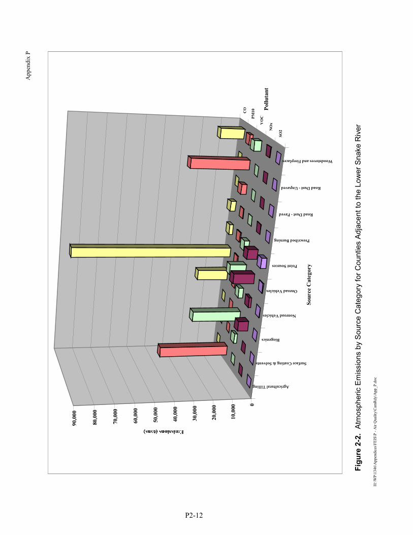
A

ppen

dix

P

H

:\WP\

1346

\App

endi

ces\

FEIS

\P -

Air

Qua

lity\

Cam

Rdy

\App

_P.d

oc

P2-12

Fi

gure

2-2

. At

mos

pher

ic E

mis

sion

s by

Sou

rce

Cat

egor

y fo

r Cou

ntie

s Ad

jace

nt to

the

Low

er S

nake

Riv

er

Agricultural Tilling

Surface Coating & Solvents

Biogenics

Nonroad Vehicles

Onroad Vehicles

Point Sources

Prescribed Burning

Road Dust - Paved

Road Dust - Unpaved

Woodstoves and Fireplaces

SO2N

OxV

OCPM

10CO

0

10,0

00

20,0

00

30,0

00

40,0

00

50,0

00

60,0

00

70,0

00

80,0

00

90,0

00

Sour

ce C

ateg

ory

Pollu

tant

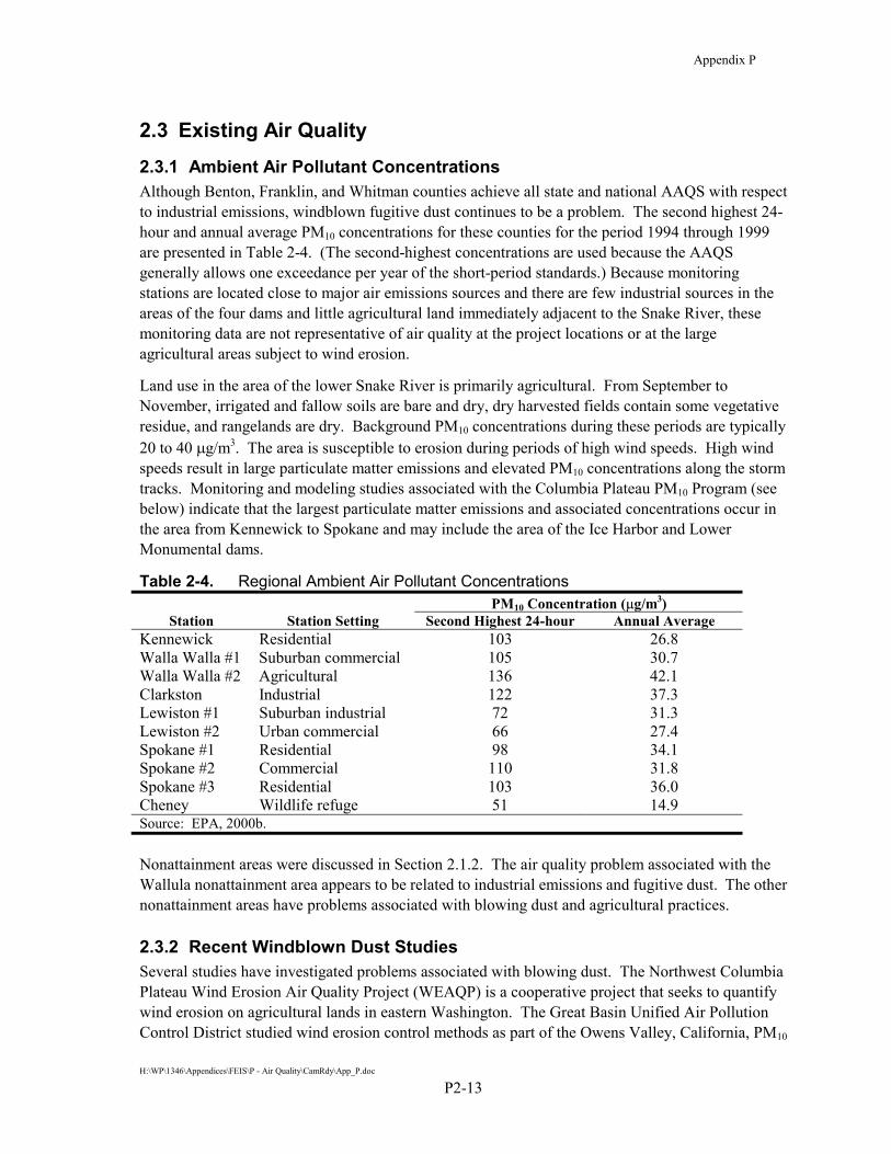
Appendix P


P2-13

2.3 Existing Air Quality 2.3.1 Ambient Air Pollutant Concentrations Although Benton, Franklin, and Whitman counties achieve all state and national AAQS with respect to industrial emissions, windblown fugitive dust continues to be a problem. The second highest 24-hour and annual average PM10 concentrations for these counties for the period 1994 through 1999 are presented in Table 2-4. (The second-highest concentrations are used because the AAQS generally allows one exceedance per year of the short-period standards.) Because monitoring stations are located close to major air emissions sources and there are few industrial sources in the areas of the four dams and little agricultural land immediately adjacent to the Snake River, these monitoring data are not representative of air quality at the project locations or at the large agricultural areas subject to wind erosion.

Land use in the area of the lower Snake River is primarily agricultural. From September to November, irrigated and fallow soils are bare and dry, dry harvested fields contain some vegetative residue, and rangelands are dry. Background PM10 concentrations during these periods are typically 20 to 40 �g/m3. The area is susceptible to erosion during periods of high wind speeds. High wind speeds result in large particulate matter emissions and elevated PM10 concentrations along the storm tracks. Monitoring and modeling studies associated with the Columbia Plateau PM10 Program (see below) indicate that the largest particulate matter emissions and associated concentrations occur in the area from Kennewick to Spokane and may include the area of the Ice Harbor and Lower Monumental dams.

Table 2-4. Regional Ambient Air Pollutant Concentrations PM10 Concentration (�g/m3)

Station Station Setting Second Highest 24-hour Annual Average Kennewick Residential 103 26.8 Walla Walla #1 Suburban commercial 105 30.7 Walla Walla #2 Agricultural 136 42.1 Clarkston Industrial 122 37.3 Lewiston #1 Suburban industrial 72 31.3 Lewiston #2 Urban commercial 66 27.4 Spokane #1 Residential 98 34.1 Spokane #2 Commercial 110 31.8 Spokane #3 Residential 103 36.0 Cheney Wildlife refuge 51 14.9 Source: EPA, 2000b. Nonattainment areas were discussed in Section 2.1.2. The air quality problem associated with the Wallula nonattainment area appears to be related to industrial emissions and fugitive dust. The other nonattainment areas have problems associated with blowing dust and agricultural practices.

2.3.2 Recent Windblown Dust Studies Several studies have investigated problems associated with blowing dust. The Northwest Columbia Plateau Wind Erosion Air Quality Project (WEAQP) is a cooperative project that seeks to quantify wind erosion on agricultural lands in eastern Washington. The Great Basin Unified Air Pollution Control District studied wind erosion control methods as part of the Owens Valley, California, PM10

Appendix P


P2-14

demonstration of attainment. The Lake Koocanusa Fugitive Dust Study measured PM10 concentrations associated with seasonal blowing dust from a western Montana lake bed. The results of these studies are summarized below.

2.3.2.1 The Columbia Plateau Wind Erosion Air Quality Project The Columbia Plateau PM10 Program (CP3) is a multi-investigator study of wind erosion and windblown dust in an area encompassing eastern Washington, northeast Oregon, and the Idaho panhandle, with an emphasis on the role of agricultural lands and regional dust storms. Typical 24-hour background PM10 concentrations measured as part of CP3 are about 34 �g/m3 in the early fall and 10 �g/m3 in the late fall. During wind events, ambient concentrations at urban receptors can exceed 500 �g/m3 on an hourly basis and 300 �g/m3 in 24 hours.

The abbreviated objectives of the CP3 include (WEAQP, 1995):

�� Develop a database of climate, soil, vegetation, and farming practices required to estimate PM10 emissions.

�� Establish the theory, quantification, and verification of wind erosion on agricultural lands, using instrumented field sites and a portable wind tunnel.

�� Develop a PM10 emissions inventory and probable urban impacts.

�� Obtain, test, and evaluate an air transport-dispersion-deposition model suitable to predict PM10 concentrations from agricultural emissions sources.

�� Identify and test wind erosion and PM10 emission control methods and evaluate their effectiveness.

�� Reclassify appropriately highly erodible lands for control and develop a strategy to set on-farm compliance and assistance.

�� Determine the relative impact of human activity on suspended dust and PM10 emission rates by determining erosion rates for non-anthropogenic and anthropogenic areas.

�� Develop an awareness and increased understanding about wind erosion, PM10 emissions, and current and prospective control methods.

�� Increase understanding of the health impacts of particulate air pollution.

�� Develop agricultural windblown dust best management practices and implementation policies.

�� Develop a particulate air quality plan to achieve solutions to PM10 problems throughout the Columbia Plateau.

The most severe windblown dust events occur during the relatively dry September to mid-November period. However, dust storms can also occur during the spring and summer. Dust storms are characterized by a surface low pressure system located in southern British Columbia or Alberta and a surface high pressure system in the southwest United States. The southwest winds generated by the low pressure system are enhanced by the clockwise flow around the high pressure system.

Appendix P


P2-15

Storms moving through eastern Washington toward the Northeast may affect an area from Kennewick to Spokane, which includes the western area of the lower Snake River. Storms that generate fugitive dust in the western region of the lower Snake River may miss the eastern reach of the river. Other storms may affect the Pendleton to Clarkston/Lewiston area.

The CP3 program investigated several storms that struck the area between 1990 and 1993. Field measurements during two major dust storms in the fall of 1993 measured maximum 24-hour PM10 concentrations equal to 300, 255, and 1,166 of �g/m3 at an industrial site in Spokane, a residential site in Spokane, and an urban site in Kennewick, respectively. A regional windblown PM10 emissions-dispersion-deposition model was calibrated with data from a portable wind tunnel. The model reasonably reproduced the measured concentrations from the fall of 1993 and was used to predict PM10 concentrations throughout the Columbia Plateau (Claiborn et al., 1998).

During the September 11, 1993, windstorm, peak wind speeds were 12.2 meters per second (m/sec) or 27 miles per hour (mph), and measured 24-hour PM10 concentrations exceeded 200 �g/m3 in Spokane and 100 �g/m3 in Kennewick. The highest modeled hourly concentration was over 2,000 �g/m3. Total emissions from dry agriculture lands, irrigated agricultural lands, and rangelands for this windstorm are estimated at 116 million metric tons (128 million tons). The emission source was near Kennewick, and the plume stretched to the northeast. During the November 3, 1993, event the winds reached 26 m/sec (58 mph). The highest measured 24-hour concentrations in Adams County reached 187 �g/m3, and the highest measured 1-hour concentration in Spokane was 440 �g/m3. Total emissions from dry agriculture lands, irrigated agricultural lands, and rangelands are estimated at 81 million metric tons (89 million tons) for this wind event. During both of these events, predicted 24-hour PM10 concentrations near the Ice Harbor and Lower Granite reservoirs were 2,400 and 50 �g/m3, respectively.

The studies conducted by CP3 are directly related to the problem of windblown dust and the impacts of dam removal. CP3 modeled several storms without the dry lower Snake River reservoirs as emission sources and recently re-ran the models including the dry reservoirs as sources, thereby helping to define impacts associated with dam breaching. As an original sponsor of the CP3 project, Ecology has received the results of the original studies. Through its public awareness and research programs, CP3 has helped increase understanding of the nature of dust-related problems in eastern Washington and has developed guidance to assist the agricultural industry in its efforts to reduce fugitive dust emissions.

2.3.2.2 The Owens Valley PM10 Demonstration of Attainment The Owens Valley PM10 Demonstration of Attainment provided information relevant to the impacts associated with drawdown. Owens Lake, located in eastern central California, is the source of large amounts of dust. The southern portion of the Owens Valley is a “serious” PM10 nonattainment area. The designation is “serious” because of frequent violations of the national AAQS and the inability of the area to attain the standards by December 31, 1995. Emissions from Owens Lake have been predicted to cause exceedances of the 24-hour AAQS up to 31 km (50 miles) away. The Great Basin Unified Air Pollution Control District published an attainment plan in 1998, which includes ambient meteorological and PM10 measurements, dust emission measurements, and the effectiveness of several control strategies.

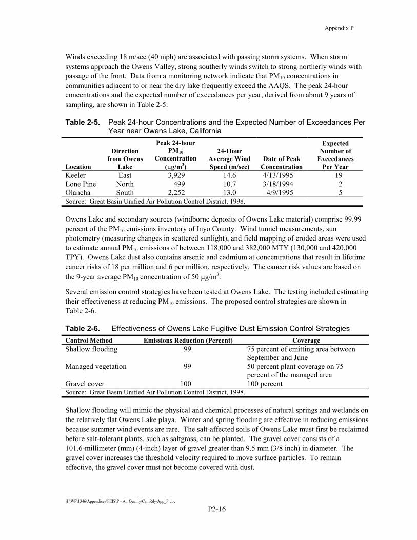
Appendix P


P2-16

Winds exceeding 18 m/sec (40 mph) are associated with passing storm systems. When storm systems approach the Owens Valley, strong southerly winds switch to strong northerly winds with passage of the front. Data from a monitoring network indicate that PM10 concentrations in communities adjacent to or near the dry lake frequently exceed the AAQS. The peak 24-hour concentrations and the expected number of exceedances per year, derived from about 9 years of sampling, are shown in Table 2-5.

Table 2-5. Peak 24-hour Concentrations and the Expected Number of Exceedances Per Year near Owens Lake, California

Location

Direction from Owens

Lake

Peak 24-hour PM10

Concentration (�g/m3)

24-Hour Average Wind Speed (m/sec)

Date of Peak Concentration

Expected Number of

Exceedances Per Year

Keeler East 3,929 14.6 4/13/1995 19 Lone Pine North 499 10.7 3/18/1994 2 Olancha South 2,252 13.0 4/9/1995 5 Source: Great Basin Unified Air Pollution Control District, 1998.

Owens Lake and secondary sources (windborne deposits of Owens Lake material) comprise 99.99 percent of the PM10 emissions inventory of Inyo County. Wind tunnel measurements, sun photometry (measuring changes in scattered sunlight), and field mapping of eroded areas were used to estimate annual PM10 emissions of between 118,000 and 382,000 MTY (130,000 and 420,000 TPY). Owens Lake dust also contains arsenic and cadmium at concentrations that result in lifetime cancer risks of 18 per million and 6 per million, respectively. The cancer risk values are based on the 9-year average PM10 concentration of 50 �g/m3.

Several emission control strategies have been tested at Owens Lake. The testing included estimating their effectiveness at reducing PM10 emissions. The proposed control strategies are shown in Table 2-6.

Table 2-6. Effectiveness of Owens Lake Fugitive Dust Emission Control Strategies Control Method Emissions Reduction (Percent) Coverage Shallow flooding 99 75 percent of emitting area between

September and June Managed vegetation 99 50 percent plant coverage on 75

percent of the managed area Gravel cover 100 100 percent Source: Great Basin Unified Air Pollution Control District, 1998.

Shallow flooding will mimic the physical and chemical processes of natural springs and wetlands on the relatively flat Owens Lake playa. Winter and spring flooding are effective in reducing emissions because summer wind events are rare. The salt-affected soils of Owens Lake must first be reclaimed before salt-tolerant plants, such as saltgrass, can be planted. The gravel cover consists of a 101.6-millimeter (mm) (4-inch) layer of gravel greater than 9.5 mm (3/8 inch) in diameter. The gravel cover increases the threshold velocity required to move surface particles. To remain effective, the gravel cover must not become covered with dust.

Appendix P


P2-17

The control strategies proposed for Owens Lake have been adopted in this appendix as demonstrated and achievable methods of reducing emissions from dry lake sediments. The Great Basin Unified Air Pollution Control District’s effort to understand and address the Owens Lake fugitive dust problem is a model for the effort that will be required in eastern Washington if the region is designated as a PM10 nonattainment area.

2.3.2.3 The Lake Koocanusa Fugitive Dust Study A recent similar study has illuminated the meteorological conditions associated with high fugitive dust events (Environalysis, 1996). PM10 monitoring was conducted at Lake Koocanusa, the reservoir formed by Libby Dam on the Kootenai River in northwestern Montana. Lake Koocanusa refills with snowpack melt in the late spring and summer. Two years of monitoring (May 1994 through June 1996) measured meteorological conditions, continuous PM10 concentrations at the lake and in the nearby town of Eureka, and passive dust settling measurements. The following meteorological conditions are associated with entrainment of fugitive dust:

�� High dust events are preceded by several hours of increasing wind speeds from a constant direction.

�� The wind speeds that initiate a dust event are not unusually high. A minimum threshold of wind energy is required to initiate the dust event.

�� The high wind events last up to 9 hours.

�� Background dust levels may significantly contribute to the measured concentrations.

�� Dust levels rapidly fall when the wind speed drops below about 5 m/sec (10 mph).

�� Dry lake banks appear to provide turbulent conditions that enhance emissions and produce more emissions.

The geography and microtopography of the dry lakebed sediments can be an important factor. Different wind patterns can affect different areas of the lakebed. Steep slopes, which allow heavier particles to roll downslope, make smaller particles available for entrainment. Although some 1-hour PM10 concentrations measured during the Lake Koocanusa study were very large, all 24-hour concentrations were lower than the air quality standard.

On several occasions, measured maximum 1-hour PM10 concentrations exceeded about 500 �g/m3. In all cases, the average 24-hour PM10 concentrations were below 100 �g/m3, or about 67 percent of the AAQS. The dust events were characterized by moderate persistent winds and dry conditions and lasted from between 3 and 9 hours. The largest measured 1-hour concentration was associated with winds that blew over large areas of exposed lake banks.

2.4 Climatic Factors Dry, loose lake sediments become airborne during high wind events. Surface particles are much less mobile if the ground is wet or frozen. The greatest potential for windblown dust coincides with periods of low relative humidity, extended sunshine, and warm to hot temperatures. The wind, precipitation, and temperature conditions of the lower Snake River region are discussed below. Monthly tabulations of climatic variables are presented in Annex A.

Appendix P


P2-18

2.4.1 Precipitation and Temperature The availability of soils that may be subject to wind erosion is partially a function of the precipitation and temperature climatology of the region. Moisture helps hold soil particles together and reduces erosion potential. Higher temperatures enhance evaporation, drying soils and providing particulate matter that may be subject to wind erosion. Soil erosion is negligible when the temperatures are below freezing.

The Cascade Mountains effectively block most precipitation from entering southeast Washington and northeast Oregon. Annual precipitation amounts are about 250 mm (10 inches) or less, with most of the precipitation falling during the winter (Figure 2-3) (Corps, 1999). Some locations in southeast Washington and northeast Oregon experience only small amounts of summer rain. Relative humidity values can fall to 10 percent or less on hot summer afternoons. Precipitation amounts generally increase with elevation and are slightly higher in the Clarkston and Lewiston area.

Climatic conditions in the lower Snake River area are characterized by large seasonal temperature differences, low precipitation, and relatively minimal cloud cover. Valley bottoms along the Snake River have the highest summer temperatures in the region, and they tend to stay slightly warmer than surrounding upland areas in the winter.

Precipitation is typically concentrated in the late fall, winter, and early spring, with more arid conditions prevailing from late spring through the summer. Precipitation reduces the availability of particulate matter susceptible to erosion during high wind speed conditions. The reservoirs on the middle and lower Snake River generally experience measurable precipitation on 90 to 120 days per year (Jackson and Kimerling, 1993).

Long-term precipitation and temperature data are available for Ice Harbor Dam, which is representative of the western Snake River area. Precipitation and temperature data from Lewiston, located about 40 km (25 miles) southeast of the Lower Granite Dam, are representative of the eastern area of the lower Snake River. In general, normal precipitation amounts increase and temperatures decrease from west to east across the lower Snake River area (Figures 2-3 and 2-4). Figures 2-3 and 2-4 are based on more than 30 years of data (NOAA, 1999 a and b).

2.4.2 Wind Conditions Air quality at specific locations within the basin is heavily influenced by wind conditions, which in turn reflect both prevailing regional patterns and local topographic factors. The prevailing wind direction in southeastern Washington is from the southwest in both winter and summer. Average wind speeds throughout the basin are generally in the range of 11 to 13 kilometers per hour (km/hour) (7 to 8 mph). Some locations have considerably higher wind speeds (Jackson and Kimerling, 1993).

Infrequent July and August thunderstorms, which usually drop only small amounts of rain, are sometimes accompanied by strong wind gusts. Winter weather conditions in the region often produce strong winds flowing across the region. Local winds in the reservoir areas are often channeled parallel to the shoreline by the river valleys. Local topography can also act as a funnel that increases wind speeds. A daily cycle of changing up-valley and down-valley local wind directions can be common, particularly in mountain areas.

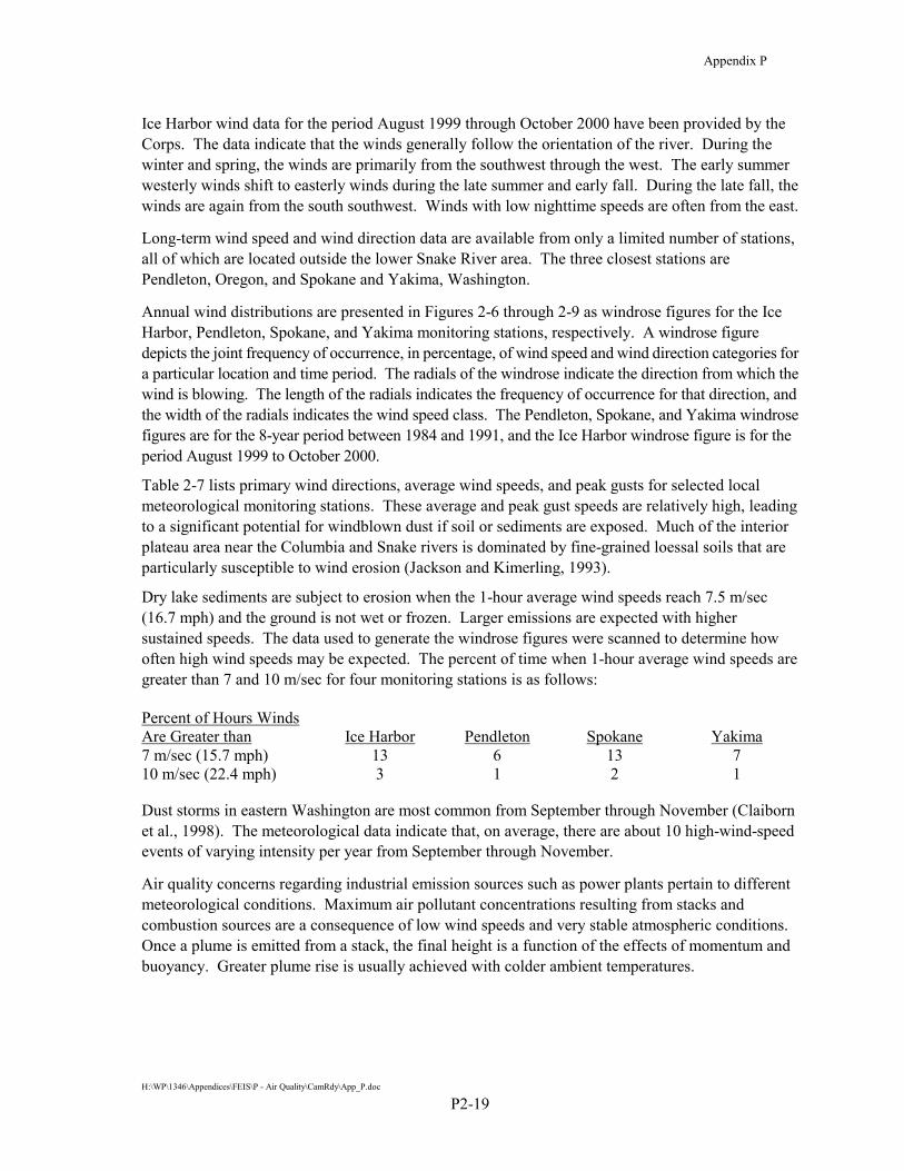
Appendix P


P2-19

Ice Harbor wind data for the period August 1999 through October 2000 have been provided by the Corps. The data indicate that the winds generally follow the orientation of the river. During the winter and spring, the winds are primarily from the southwest through the west. The early summer westerly winds shift to easterly winds during the late summer and early fall. During the late fall, the winds are again from the south southwest. Winds with low nighttime speeds are often from the east.

Long-term wind speed and wind direction data are available from only a limited number of stations, all of which are located outside the lower Snake River area. The three closest stations are Pendleton, Oregon, and Spokane and Yakima, Washington.

Annual wind distributions are presented in Figures 2-6 through 2-9 as windrose figures for the Ice Harbor, Pendleton, Spokane, and Yakima monitoring stations, respectively. A windrose figure depicts the joint frequency of occurrence, in percentage, of wind speed and wind direction categories for a particular location and time period. The radials of the windrose indicate the direction from which the wind is blowing. The length of the radials indicates the frequency of occurrence for that direction, and the width of the radials indicates the wind speed class. The Pendleton, Spokane, and Yakima windrose figures are for the 8-year period between 1984 and 1991, and the Ice Harbor windrose figure is for the period August 1999 to October 2000.

Table 2-7 lists primary wind directions, average wind speeds, and peak gusts for selected local meteorological monitoring stations. These average and peak gust speeds are relatively high, leading to a significant potential for windblown dust if soil or sediments are exposed. Much of the interior plateau area near the Columbia and Snake rivers is dominated by fine-grained loessal soils that are particularly susceptible to wind erosion (Jackson and Kimerling, 1993).

Dry lake sediments are subject to erosion when the 1-hour average wind speeds reach 7.5 m/sec (16.7 mph) and the ground is not wet or frozen. Larger emissions are expected with higher sustained speeds. The data used to generate the windrose figures were scanned to determine how often high wind speeds may be expected. The percent of time when 1-hour average wind speeds are greater than 7 and 10 m/sec for four monitoring stations is as follows:

Percent of Hours Winds Are Greater than Ice Harbor Pendleton Spokane Yakima 7 m/sec (15.7 mph) 13 6 13 7 10 m/sec (22.4 mph) 3 1 2 1

Dust storms in eastern Washington are most common from September through November (Claiborn et al., 1998). The meteorological data indicate that, on average, there are about 10 high-wind-speed events of varying intensity per year from September through November.

Air quality concerns regarding industrial emission sources such as power plants pertain to different meteorological conditions. Maximum air pollutant concentrations resulting from stacks and combustion sources are a consequence of low wind speeds and very stable atmospheric conditions. Once a plume is emitted from a stack, the final height is a function of the effects of momentum and buoyancy. Greater plume rise is usually achieved with colder ambient temperatures.

brownj

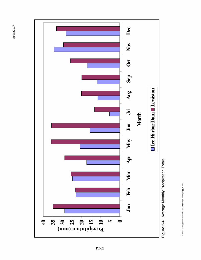
A

ppen

dix

P

H

:\WP\

1346

\App

endi

ces\

FEIS

\P -

Air

Qua

lity\

Cam

Rdy

\App

_P.d

oc

P2-21

Figu

re 2

-4.

Aver

age

Mon

thly

Pre

cipi

tatio

n To

tals

0510152025303540

Jan

Feb

Mar

Apr

May

Jun

Jul

Aug

Sep

Oct

Nov

Dec

Mon

th

Precipitation (mm)

Ice H

arbo

r Dam

Lewi

ston

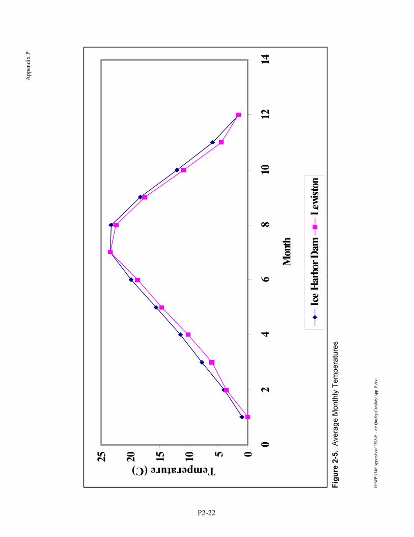
A

ppen

dix

P

H

:\WP\

1346

\App

endi

ces\

FEIS

\P -

Air

Qua

lity\

Cam

Rdy

\App

_P.d

oc

P2-22

Figu

re 2

-5.

Aver

age

Mon

thly

Tem

pera

ture

s

0510152025

02

46

810

1214

Mon

th

Temperature (C)

Ice H

arbo

r Dam

Lewi

ston

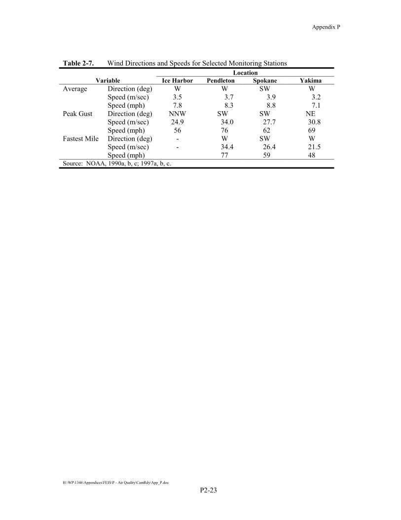
Appendix P


P2-23

Table 2-7. Wind Directions and Speeds for Selected Monitoring Stations

Location Variable Ice Harbor Pendleton Spokane Yakima

Average Direction (deg) W W SW W Speed (m/sec) 3.5 3.7 3.9 3.2 Speed (mph) 7.8 8.3 8.8 7.1 Peak Gust Direction (deg) NNW SW SW NE Speed (m/sec) 24.9 34.0 27.7 30.8 Speed (mph) 56 76 62 69 Fastest Mile Direction (deg) - W SW W Speed (m/sec) - 34.4 26.4 21.5 Speed (mph) 77 59 48 Source: NOAA, 1990a, b, c; 1997a, b, c.

Appendix P


P2-24

Figure 2-6. Ice Harbor, Washington Windrose for August 1999�October 2000

Appendix P


P2-25

Figure 2-7. Pendleton, Oregon Windrose for 1984�1991

Appendix P


P2-26

Figure 2-8. Spokane, Washington Windrose for 1984�1991

Appendix P


P2-27

Figure 2-9. Yakima, Washington Windrose for 1984�1991

Appendix P


P3-1

3. Study Methods Section 3 presents the methods used in this analysis of the air quality impacts associated with the Feasibility Study alternatives. This analysis addresses the four impact issues identified in Section 1:

�� Fugitive dust emissions resulting from demolition of the dams

�� The change in transportation-related emissions

�� Effects of fugitive dust

�� Emissions associated with replacing lost hydropower.

Under the Dam Breaching alternative, the lower Snake River dams would be breached. Demolition activities such as hauling and dumping fill material would generate fugitive emissions. Section 3.1 presents methods used to estimate construction-related fugitive emissions.

Between 2.7 million and 3.6 million metric tons (3 and 4 million tons) of freight pass through Ice Harbor Dam every year. Towboats emit pollutants along the length of the river from the confluence of the Columbia and Snake rivers to Lewiston, Idaho. The Dam Breaching alternative would require a transfer of river freight to rails and roads, changing the amount and distribution of traffic-related air emissions. Section 3.2 presents the methods used to estimate the change in transportation-related emissions.

Wind-generated dust originating from dry reservoir sediments could be a problem in areas adjacent to the reservoirs. Limited monitoring data are available to characterize emissions from dry lake beds. As an alternative, a method for predicting the amount of particulate matter (PM10) emitted during high wind speed events is presented (Section 3.3).

The Dam Breaching alternative would require replacement of hydropower through increased power generation from existing plants or construction of new power-generating capacity. Replacement of hydropower would increase atmospheric emissions of criteria air pollutants, HAPs, and GHGs. Section 3.4 presents the methods used to estimate emissions associated with replacement hydropower.

3.1 Demolition Fugitive Emissions In terms of atmospheric emissions, excavation and deconstruction of the lower Snake River dams would be equivalent to a large construction project. According to the Natural River Drawdown Engineering Appendix (Appendix D), demolition will be conducted in 2 years. However, deconstruction could last longer, depending on the project schedule and whether one or more dams are demolished simultaneously. This analysis conservatively assumes that all four projects are demolished in 1 year. In addition, emissions associated with rock quarried for embankment repairs, drainage structure protection, and level fill are included.

The principal construction operations that generate fugitive dust include unloading material from trucks and hauling, bulldozing, and grading the material. Construction activities are generalized into bulldozing, batch dropping, hauling on unpaved roads, and grading. The analysis estimates fugitive dust emissions and the resulting ambient concentrations.

Appendix P


P3-2

3.1.1 Emission Calculations Emissions have been estimated for embankment and abutment excavations and construction and diversion levees. In addition, emissions associated with quarry excavation for levee stabilization have been estimated.

3.1.1.1 Embankment and Abutment Excavation Emission Estimates Equations for estimating construction-related emissions are available from EPA (1998). The emission factor equations are based on material handling rates, soil moisture content, silt content, and other factors such as vehicle weight and wind speed. The expressions include dimensionless multipliers to account for aerodynamic particle size. For this study, multipliers for PM10 have been incorporated into the equations. The equations also include the mitigating effects of rain. The emission factor expressions used in this study are presented in Table 3-1. Bulldozer emissions are expressed in units of kilograms per hour (kg/hour). Hauling and grading emission factors are expressed in terms of vehicle kilometers traveled (VKT). Dropping emission factors are in terms of the amount of material in metric tons (MT).

Table 3-1. Fugitive Dust Emission Equations

Operation EPA, 1998 Reference Units Equation

Bulldozing Table 11.9-2 kg/hour EFB = 0.75 * (0.45 * (s1.5 /M1.4) * (365-p)/365

Hauling Section 13.2.2 g/VKT EFH = 281.9 * (2.6 * (s/12)0.8(W/3)0.4) / (M/0.2)0.3 * (365-p)/365

Dropping Section 13.2.4 kg/MT EFD = 0.35 * 0.0016 * (u/2.2)1.3 / (M/2)1.4 * (365-p)/365

Grading Table 11.9-2 kg/VKT EFG = 0.60 * 0.0056 * S2.0 * (365-p)/365

Where: M = moisture content, in percent

p = number of days with measurable precipitation

s = silt content, in percent

S = mean vehicle speed, in km/hour

u = mean wind speed, in m/sec

W = mean vehicle weight, in metric tons. Source: EPA, 1998.

Annual fugitive emissions of PM10 are estimated for bulldozing, loading, hauling, dumping, and grading operations for each project, based on the amount of soil and fill material that must be moved to breach the dams. The emission calculations require volume of material, road lengths, and average weight of the haul trucks. The analysis does not include vehicle tailpipe emissions or emissions from worker camps. The default values for constants used in the emission calculations are presented in Table 3-2.

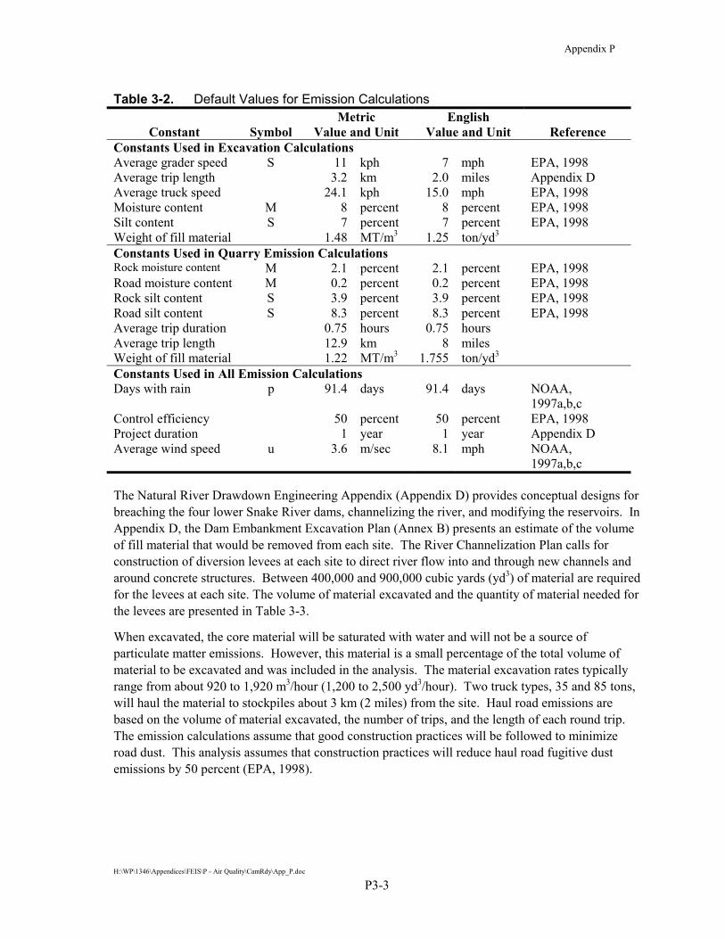
Appendix P


P3-3

Table 3-2. Default Values for Emission Calculations Metric English

Constant Symbol Value and Unit Value and Unit Reference Constants Used in Excavation Calculations Average grader speed S 11 kph 7 mph EPA, 1998 Average trip length 3.2 km 2.0 miles Appendix D Average truck speed 24.1 kph 15.0 mph EPA, 1998 Moisture content M 8 percent 8 percent EPA, 1998 Silt content S 7 percent 7 percent EPA, 1998 Weight of fill material 1.48 MT/m3 1.25 ton/yd3 Constants Used in Quarry Emission Calculations Rock moisture content M 2.1 percent 2.1 percent EPA, 1998 Road moisture content M 0.2 percent 0.2 percent EPA, 1998 Rock silt content S 3.9 percent 3.9 percent EPA, 1998 Road silt content S 8.3 percent 8.3 percent EPA, 1998 Average trip duration 0.75 hours 0.75 hours Average trip length 12.9 km 8 miles Weight of fill material 1.22 MT/m3 1.755 ton/yd3 Constants Used in All Emission Calculations Days with rain p 91.4 days 91.4 days NOAA,

1997a,b,c Control efficiency 50 percent 50 percent EPA, 1998 Project duration 1 year 1 year Appendix D Average wind speed u 3.6 m/sec 8.1 mph NOAA,

1997a,b,c

The Natural River Drawdown Engineering Appendix (Appendix D) provides conceptual designs for breaching the four lower Snake River dams, channelizing the river, and modifying the reservoirs. In Appendix D, the Dam Embankment Excavation Plan (Annex B) presents an estimate of the volume of fill material that would be removed from each site. The River Channelization Plan calls for construction of diversion levees at each site to direct river flow into and through new channels and around concrete structures. Between 400,000 and 900,000 cubic yards (yd3) of material are required for the levees at each site. The volume of material excavated and the quantity of material needed for the levees are presented in Table 3-3.

When excavated, the core material will be saturated with water and will not be a source of particulate matter emissions. However, this material is a small percentage of the total volume of material to be excavated and was included in the analysis. The material excavation rates typically range from about 920 to 1,920 m3/hour (1,200 to 2,500 yd3/hour). Two truck types, 35 and 85 tons, will haul the material to stockpiles about 3 km (2 miles) from the site. Haul road emissions are based on the volume of material excavated, the number of trips, and the length of each round trip. The emission calculations assume that good construction practices will be followed to minimize road dust. This analysis assumes that construction practices will reduce haul road fugitive dust emissions by 50 percent (EPA, 1998).

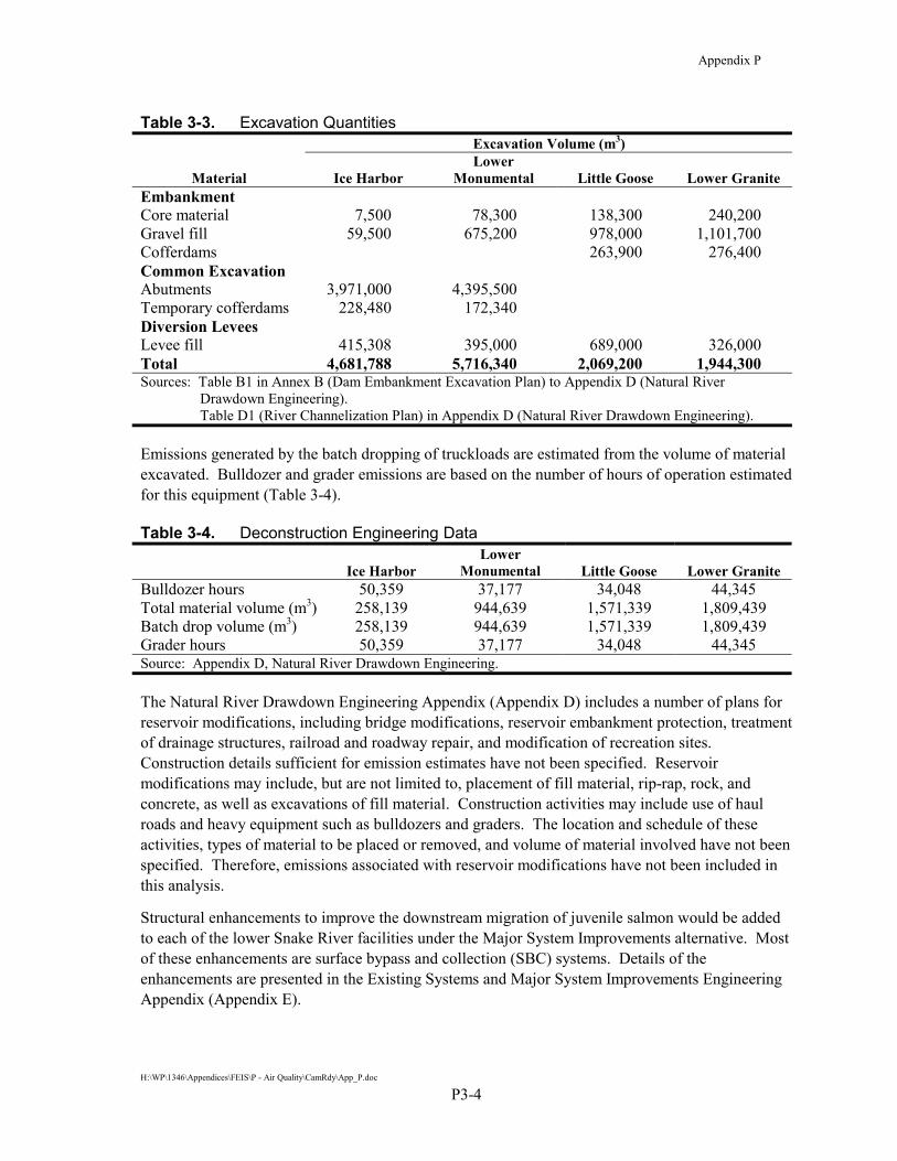
Appendix P


P3-4

Table 3-3. Excavation Quantities Excavation Volume (m3)

Material Ice Harbor Lower

Monumental Little Goose Lower Granite Embankment Core material 7,500 78,300 138,300 240,200 Gravel fill 59,500 675,200 978,000 1,101,700 Cofferdams 263,900 276,400 Common Excavation Abutments 3,971,000 4,395,500 Temporary cofferdams 228,480 172,340 Diversion Levees Levee fill 415,308 395,000 689,000 326,000 Total 4,681,788 5,716,340 2,069,200 1,944,300 Sources: Table B1 in Annex B (Dam Embankment Excavation Plan) to Appendix D (Natural River

Drawdown Engineering). Table D1 (River Channelization Plan) in Appendix D (Natural River Drawdown Engineering).

Emissions generated by the batch dropping of truckloads are estimated from the volume of material excavated. Bulldozer and grader emissions are based on the number of hours of operation estimated for this equipment (Table 3-4).

Table 3-4. Deconstruction Engineering Data

Ice Harbor Lower

Monumental Little Goose Lower Granite Bulldozer hours 50,359 37,177 34,048 44,345 Total material volume (m3) 258,139 944,639 1,571,339 1,809,439 Batch drop volume (m3) 258,139 944,639 1,571,339 1,809,439 Grader hours 50,359 37,177 34,048 44,345 Source: Appendix D, Natural River Drawdown Engineering.

The Natural River Drawdown Engineering Appendix (Appendix D) includes a number of plans for reservoir modifications, including bridge modifications, reservoir embankment protection, treatment of drainage structures, railroad and roadway repair, and modification of recreation sites. Construction details sufficient for emission estimates have not been specified. Reservoir modifications may include, but are not limited to, placement of fill material, rip-rap, rock, and concrete, as well as excavations of fill material. Construction activities may include use of haul roads and heavy equipment such as bulldozers and graders. The location and schedule of these activities, types of material to be placed or removed, and volume of material involved have not been specified. Therefore, emissions associated with reservoir modifications have not been included in this analysis.

Structural enhancements to improve the downstream migration of juvenile salmon would be added to each of the lower Snake River facilities under the Major System Improvements alternative. Most of these enhancements are surface bypass and collection (SBC) systems. Details of the enhancements are presented in the Existing Systems and Major System Improvements Engineering Appendix (Appendix E).

Appendix P


P3-5

The SBC structures would be built in place or would be built offsite and assembled onsite. Assuming that onsite construction would be employed, the emission sources for the Major System Improvements alternative include construction-related activities such as cement mixing and unpaved road emissions. Small emissions would result from loading cement, sand, aggregate, and water into mixer trucks. Particulate matter, primarily cement dust from the mixer trucks, is the pollutant of concern. EPA emission factors for truck-mixed concrete are 0.01 kg/MT of cement (0.04 lb/yd3) (EPA, 1998, Table 11.12-2 dated 10/86).

Construction-related emissions for the Major System Improvements alternative would be very small. To provide emission quantities for a comparison of the alternatives, construction-related emissions have been assumed to equal 1 MTY (1 TPY) for all four hydrofacilities. While unknown at this time, it is possible that modifications in farming patterns due to regional economic changes (such as shifts from irrigated to dryland farming) could also lead to changes in emissions.

3.1.1.2 Quarry Excavation Emission Estimates The quarries will be used until all rock necessary for embankment repairs, drainage structure protection, and levee fill is obtained. This analysis assumes that all quarries will operate for one full year. The principal operations that generate fugitive dust are crushing and screening material, loading and unloading material on trucks, and hauling on unpaved roads.

Equations for construction-related emission factors as well as crushed stone processing are available from EPA (1998). The emission factor equations are based on material handling rates, soil moisture content, silt content, and other factors, such as vehicle weight and wind speed. The expressions include dimensionless multipliers to account for aerodynamic particle size. For this study, multipliers for PM10 have been incorporated into the equations. The equations also include the mitigating effects of rain. The emission factor expressions used in this study are the same as those presented in Table 3-1.

Annual fugitive emissions of PM10 are estimated for screening and crushing rock, and loading, hauling, and dumping operations for each quarry, based on the amount of rock that must be processed at each quarry. The emission calculations require volume of material, road lengths, and average weight of the haul trucks. The calculations also include hauling and dumping during final placement of the material. The analysis does not include vehicle tailpipe emissions or emissions from worker camps. The default values for constants used in the emission calculations are presented in Table 3-2.

The Natural River Drawdown Engineering Appendix (Appendix D) provides conceptual designs for breaching the four lower Snake River dams, river channelization, and reservoir modifications. Annex D to Appendix D, the River Channelization Plan, provides an estimate of the volume of levee fill material required. Annex F, the Railroad and Highway Embankment Protection Plan, presents an estimate of the volume of fill material required for embankment modification. Annex G, the Drainage Structures Protection Plan, provides information regarding the amount of material required for drainage structure protection. Annex H, the Railroad and Roadway Damage Repair Plan, presents an estimate of the amount of fill needed for road and railroad embankment repairs. The total volume of material needed from each quarry is presented in Table 3-5. Quarry excavations will take place over a period of 3 years. However, to be consistent and comparable with the other emission estimates, this estimate assumes that the excavations will be completed in 1 year. This is

Appendix P


P3-6

Table 3-5. Quarry Excavation Quantities Excavation Quantities (m3)

Quarry and River Mile Destination

Quarry 1 (RM20) Ice Harbor Area

Quarry 2 (RM60) Lower Monumental

and Little Goose Areas Quarry 3 (RM133)

Lower Granite Area Levee fill material 326,000 1,084,000 415,308Reservoir embankment modification

200,566 411,664 288,823

Road/railroad repairs 156,682 418,336 362,090Drainage structures 2,900 5,304 4,427Total 686,149 1,919,306 1,070,651

also done to try and understand how extensive the effects might be if quarrying was, for some reason, done in a 1-year period. This approach is consistent with EPA screening procedures (see Section 3.1.2).

The amount of fill material excavated from the quarries will be about 2 to 3 times greater than the amount of material needed. For this analysis, it was assumed that the volume of material processed is 3 times greater than the volume of material needed. Two truck types, 35T and 85T, will haul the material about 13 km (8 miles) to barges at the river (the exact distances of the quarries from the river have not been specified). Haul road emissions assume that the roads are unpaved and are based on the volume of material quarried, the number of trips, and the length of each round trip. The emission calculations assume that good construction practices will be followed to minimize road dust. This emission estimate assumes that construction practices will reduce haul road fugitive dust emissions by 50 percent.

Emissions generated by screening and crushing quarried material are based on EPA emission factors and the volume of material processed. Emissions generated by the batch dropping of truckloads are estimated from the volume of material required from each quarry.

Quarried material will be stockpiled in several locations along the river before being hauled to its final placement location. Primary sources of emissions are hauling and dumping of the material. The number of trips necessary for final placement of the material has been estimated in this analysis.

3.1.2 Construction Fugitive Dust Modeling The largest quantity of excavation materials and thus the largest amount of PM10 emissions are associated with demolition of the Lower Monumental Dam and excavations at Quarry 2, located near river mile (RM) 60 (Tables 3-3 and 3-5). The haul roads are the largest single source of emissions. To obtain a rough estimate of ambient concentrations associated with the excavations, PM10 emissions from haul road segments and the stockpiles were modeled. Portions of an existing road near the Lower Monumental Dam were modeled. A hypothetical haul road from Quarry 2 to the river was also modeled. Because it is not known where public access will be restricted during demolition, the 24-hour average downwind concentrations have been contoured and plotted rather than simply presented as the maximum predicted concentration.

Excavated material at Lower Monumental will be placed in three stockpiles (Appendix D, Annex B). An existing road used to access the up-slope stockpile was modeled. Other haul roads

Appendix P


P3-7

will be used to construct levees and temporary cofferdams. This analysis assumed that one-half of all the excavated material passes over the modeled road.

Using the excavation schedule of 1,100 hours (55 days, 20-hour working days, Appendix D, Annex B), the estimated Lower Monumental haul road emissions were converted to units of grams per second per square meter (g/sec-m2). The stockpile emission rates assume that one-half of the bulldozer, dumping, and grading emissions originate from the two large stockpiles. The quarry modeling assumed that the estimated emissions occurred over a 3-year period.

It is not necessary to model an entire road to predict excavation concentrations because maximum concentrations are adjacent to the fugitive dust sources. Emissions from the Lower Monumental haul road segments and stockpiles were modeled with ISCST3 (EPA, 1995c). Likewise, only a portion of a hypothetical quarry haul road was also modeled with ISCST3. According to the Guideline on Air Quality Models (40CFR Part 51 Appendix W), ISCST3 is appropriate for modeling regulated air pollutants from area sources in complex configurations. ISCST3 model options were consistent with the Guideline on Air Quality Models.

The modeling used meteorological data designed to produce the maximum possible concentration, consistent with EPA’s screening procedures (EPA, 1992b). The worst case meteorology consisted of 54 combinations of wind speed and stability class for each of 36 wind directions. The modeling did not consider the frequency of occurrence of the conditions that are predicted to result in the maximum concentrations. One-hour concentrations were predicted at receptors located between the haul road and areas accessible to the public. The 1-hour concentrations were multiplied by EPA’s time conversion factors (EPA, 1992b) to produce 24-hour concentrations, which were compared to the ambient air quality standard.

The quarry haul roads are also sources of PM10 emissions. The Quarry 2 haul road was modeled following the methodology presented above. In this case, it was assumed that quarry activities will continue for 3 years. A 4-mile haul road, with the excavation, rock crushing, and screening area on one end and the barge loading facility on the other end, was modeled using ISCST3 and worst-case meteorology. Results of the evaluation are presented as a contour plot of the maximum 24-hour PM10 concentrations.

Air quality regulations require that significant new sources not affect nonattainment areas without offsetting their emissions. To determine whether deconstruction emissions resulted in 24-hour concentrations greater than the 5 �g/m3 significance level, Ice Harbor Dam, stockpiles, and haul roads were modeled as several large area sources. Input data included 6 years of hourly Yakima meteorological data. Maximum 24-hour concentrations were predicted for a line of receptors south of the construction site. Results are presented as a plot of concentration versus downwind distance.

The Snake River dam breaching effort is easier to visualize if it can be compared to similar projects. However, there are few dam removal projects available for comparison. The Elwha and Glines Canyon dams, located in the Olympic National Park, are slated for demolition. The Restoration Implementation Plan Environmental Impact Statement estimated haul road emissions and resulting ambient concentrations associated with the demolition of the two dams (National Park Service, 1996). The impacts associated with lower Snake River dam demolition will be compared to those of the Elwha and Glines dams. Demolition of the Lower Monumental dam would require excavation

Appendix P


P3-8

of 30 times more material than demolition of both the Elwha and Glines Canyon dams. Air quality impacts associated with both projects are comparable.

3.2 Loss of Barge Traffic In 1994, over 3.8 million metric tons (4.2 million tons) of freight passed through the locks at Ice Harbor Dam (Lee and Casavant, 1996). Nearly all of this commerce was downriver transportation of farm products. Waterborne transportation is characterized as follows:

�� Farm products comprise 81 percent of the downriver transport and 78 percent of the total commerce.

�� Forest products comprise 16 percent of the downriver transport and 15 percent of the total commerce.

�� Petroleum products comprise 70 percent of the upriver transport and 3 percent of the total commerce.

�� Fertilizers and chemical products comprise 14 percent of the upriver transport and less than 1 percent of the total commerce.

�� Manufactured products comprise 14 percent of the upriver transport and 3 percent of the total commerce.

The Dam Breaching alternative would require a shift from barge transportation to train and truck transportation, which would change the quantity and distribution of vehicle emissions. Air emissions are estimated from the number of river, train, and road miles required to transport commodities affected by the Dam Breaching alternative. Data for this analysis are available from two sources. The Eastern Washington Intermodal Transportation Study (EWITS) conducted a number of studies, including an examination of energy consumption and air emissions associated with Snake River dam breaching. The Transportation Analysis (DREW, 1999b) provides the number of train and truck bushel-miles needed to transport the wheat and barley harvest following breaching. In addition, the change in the number of trucks hauling wheat and barley on selected Washington highways has been estimated.

3.2.1 Eastern Washington Intermodal Transportation Study EWITS is a 6-year study jointly funded by the Federal government and the Washington State Department of Transportation. EWITS was established to facilitate existing regional and state-wide transportation efforts, forecast freight and passenger transportation service needs for eastern Washington, identify gaps in eastern Washington’s current transportation infrastructure, and pinpoint transportation system improvement options critical to economic competitiveness and mobility. Data presented in several EWITS reports were incorporated into this emissions analysis.

EWITS examined the energy consumption and air emission impacts associated with Snake River dam breaching (Lee and Casavant, 1998). The study calculated the energy used and emissions created by three transportation modes (barge, train, and truck) for the 1994 eastern Washington wheat and barley harvest. Two cases were investigated: a base case modeled transportation modes currently available, and the second case examined the effects of not having barges available on the Snake River. The modeling was accomplished by using a Geographic Information System (GIS) database and a General Algebraic Modeling System (GAMS) optimization system. The GIS/GAMS

Appendix P


P3-9

model determines minimum distances and least-cost routes and modes to transport wheat and barley from farms to Portland. The model organizes the data by ton-mile of wheat and barley, sorted by transportation mode. Energy consumption and emissions factors are expressed in units of ton-miles.

Comprehensive transportation modeling would account for a number of conditions, including vehicular performance, weight factors, infrastructure quality, pre- and post-trips, and climatic conditions. The GIS/GAMS modeling accounted for several of these factors. The Lee and Casavant study included two truck types, single unit three-axle trucks and combination tractor and trailer five-axle units, differentiated by their tare weight. Locomotive energy consumption and emissions data available from literature were used in the study (EPA, 1997b). Branch line locomotives are assumed to have the same characteristics as main line locomotives.

Comprehensive marine vessel emissions were not readily available until Lloyds Register published the results of a testing program in 1995. Additional emission testing has been conducted in California, Vancouver, B.C., and on Coast Guard vessels. Marine emissions are a function of vessel deadweight, engine horsepower, speed (for example, idle, maneuvering, cruise), and load. Towboat emissions used in the EWITS modeling are compatible with the following:

�� British Columbia Ferries Emissions Test Program, by G. Rideout for the Environment Canada in 1998

�� Commercial Marine Vessel Contributions to Emission Inventories, by Booz Allen & Hamilton for the EPA in 1991

�� Emission Testing of Nonroad Compression Ignition Engines, by J. N. Carroll and C. M. Urban of the Southwest Research Institute for the EPA in 1995

�� Port of Vancouver Marine Vessel Emissions Test Project, by G. Rideout and E. Radloff for the Environment Canada in 1997

�� Shipboard Marine Engine Emission Testing for the United States Coast Guard, by Environmental Transportation Consultants for the Volpe National Transportation System Center and the United States Coast Guard Headquarters Navel Engineering Division.

Energy consumed and emissions from pre- and post-trip moves are ignored in the modeling study. Speed and road gradients are also not taken into account in the modeling. The model assumed that the entire crop was transferred to the Portland, Oregon, area for export, with no grain retained in storage. The model does not account for the possibility of railcar shortages. Finally, the study examined only the transportation of wheat and barley from the eastern Washington producing areas to the Portland seaport.

Air pollutant emission factors for diesel-fueled engines, available from EPA and others, are presented in units of pound of emitted pollutant per gallon of fuel (lb/gal). The uncontrolled emission factors were derived from EPA procedures for preparing mobile source emission inventories, and are presented in Table 3-6. Fuel usage for locomotives, trucks, and towboats were reported as the amount of energy required to move 0.9 metric tons (1 ton) of a commodity 1.6093 km (2 miles) (Btu/ton-mile). A British thermal unit (Btu) is the amount of energy required to raise the temperature of one pound of water one degree Fahrenheit (ºF). One gallon of diesel fuel is equivalent to about 137,000 BTUs. Energy requirements by transportation mode are presented in Table 3-7. The Lee and Casavant study used uncontrolled emission rates.

Appendix P


P3-10

Table 3-6. Mobile Source Emission Factors Emission Factors (lb/gal)

Mode CO VOC NOx PM10 SO2 Towboat 0.057 0.019 0.419 0.009 0.075 Locomotive 0.059 0.022 0.564 0.015 0.036 Truck, 3-axle 0.023 0.212 0.093 0.014 0.005 Truck, 5-axle 0.023 0.212 0.093 0.016 0.006 Sources: EPA, 1985, 1992, and 1997b; Lee and Casavant, 1998.

Table 3-7. Energy Requirements by Transportation Mode Mode Energy Requirement (Btu/ton-mile) Towboat 374 Locomotive 372 Truck 551 Source: Lee and Casavant, 1998.

Air pollutant emissions for each transportation mode are determined as follows:

Eap = EFap * T * M * EC / 137,000 Btu/gal

where:

Eap is the emission for each air pollutant, in lb

EFap is the emission factor for each air pollutant, in lb/gal (from Table 3-6)

T is the total tonnage for the transportation mode

M is the number of miles, and

EC is the energy consumed in Btu/ton-mile (from Table 3-7).

The GIS/GAMS model determined the optimal roads required to transport the grain harvest to elevators, the number of vehicles required to transport the harvest, and the emissions resulting from the trucks. Grain transportation from elevators to rail and river terminals and on to terminals in the Portland area was also simulated. Emissions from each transportation mode were summed. Total towboat, locomotive, and truck emissions, with and without the lower Snake River as a navigable waterway, were determined and are presented in Tables 3-8 and 3-9.

Table 3-8. Ton-miles for the 1994 Wheat and Barley Harvest with Snake River Barge Transportation

Mode Wheat (million ton-miles) Barley (million ton-miles) Barge 827.4 76.3 Train 281.9 0.037 Truck 383.5 52.1 Total 1,492.8 128.4 Source: Lee and Casavant, 1998.

Appendix P


P3-11

Table 3-9. Ton-miles for the 1994 Wheat and Barley Harvest without the Snake River Barge Transportation

Mode Wheat (million ton-miles) Barley (million ton-miles) Barge 503.2 55.8 Train 545.5 0.093 Truck 442.8 108.1 Total 1,491.5 164.0 Source: Lee and Casavant, 1998.

Wheat and barley ton-miles were used to estimate transportation emissions. Wheat and barley currently accounts for about 80 percent of the Snake River commerce, all of which would be shifted to highways and railroads. By the time dam breaching and deconstruction become effective (2010), the amount of commodities normally shipped on the waterway is projected to increase. Furthermore, containers used to transport grain are often returned to the grain-producing areas empty. Therefore, to account for empty backhauls and provide a level of conservatism, the emissions were doubled. To account for all shipped commodities and the projected increase in shipments by 2010, the emissions were increased by 13 percent.

Although vehicles are sources of small amounts of GHG and HAP emissions, little data are available to quantify these emissions. EPA has CO2 and organic compound emission factors for diesel fuel used in small stationary engines (EPA, 1998, Table 3.3-2 dated 10/96). These emission factors may be used to obtain order-of-magnitude estimates of the change in CO2, benzene, and formaldehyde emissions with drawdown. According to the emission factors, CO2 emissions are about 88 times larger than CO emissions. Benzene and formaldehyde emissions are about 0.003 times the vehicle VOC emissions, including exhaust, evaporative, crankcase, and refueling emissions.

3.2.2 Transportation Analysis The Transportation Analysis (DREW, 1999b) is an assessment of the economic effects of dam breaching on regional transportation, including alternative shipping modes and costs, and a determination of the least-cost combination of storage, handling, and transport modes which would emerge in response to curtailment of waterborne transport. The economic analysis followed these steps:

�� Identify the origins and destinations of commodity groups that use the lower Snake River.

�� Develop costs for barge, train, and truck modes from transportation analysis models.

�� Estimate transportation costs associated with the Existing Conditions and Dam Breaching alternatives with the assistance of a computer model.

Off-river origins of grain transported on the lower Snake River include areas within northeastern Oregon, eastern Washington, northern Idaho, and a small number of counties in the grain-producing areas of Montana and North Dakota. The economic analysis predicted barge bushel-miles for the Columbia and Snake Rivers before dam breaching and the change in barge, train, and truck bushel-miles after dam breaching. Following dam breaching, transportation on the Columbia River will continue. The bushel-mile data, generated by the transportation analysis and based on projected grain shipments for 2007, are presented in Table 3-10. Idaho truck bushel-miles are predicted to decrease as grain is hauled to closer elevators next to the railroads. The bushel-mile data are used to

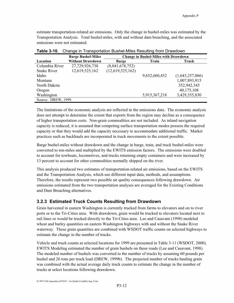
Appendix P


P3-12

estimate transportation-related air emissions. Only the change in bushel-miles was estimated by the Transportation Analysis. Total bushel-miles, with and without dam breaching, and the associated emissions were not estimated.

Table 3-10. Change in Transportation Bushel-Miles Resulting from Drawdown Barge Bushel-Miles Change in Bushel-Miles with Drawdown

Location Without Drawdown Barge Train Truck Columbia River 27,729,926,730 (8,041,678,752) Snake River 12,619,525,162 (12,619,525,162) Idaho 9,652,660,452 (1,643,257,066) Montana 1,007,893,915 North Dakota 352,942,345 Oregon 40,175,108 Washington 5,915,367,218 3,429,355,830 Source: DREW, 1999.

The limitations of the economic analysis are reflected in the emissions data. The economic analysis does not attempt to determine the extent that exports from the region may decline as a consequence of higher transportation costs. Non-grain commodities are not included. As inland navigation capacity is reduced, it is assumed that competing surface transportation modes possess the required capacity or that they would add the capacity necessary to accommodate additional traffic. Market practices such as backhauls are incorporated in truck movements to the extent possible.

Barge bushel-miles without drawdown and the change in barge, train, and truck bushel-miles were converted to ton-miles and multiplied by the EWITS emission factors. The emissions were doubled to account for towboats, locomotives, and trucks returning empty containers and were increased by 13 percent to account for other commodities normally shipped on the river.

This analysis produced two estimates of transportation-related air emissions, based on the EWITS and the Transportation Analysis, which use different input data, methods, and assumptions. Therefore, the results represent two possible air quality consequences following drawdown. Air emissions estimated from the two transportation analyses are averaged for the Existing Conditions and Dam Breaching alternatives.

3.2.3 Estimated Truck Counts Resulting from Drawdown Grain harvested in eastern Washington is currently trucked from farms to elevators and on to river ports or to the Tri-Cities area. With drawdown, grain would be trucked to elevators located next to rail lines or would be trucked directly to the Tri-Cities area. Lee and Casavant (1998) modeled wheat and barley quantities on eastern Washington highways with and without the Snake River waterway. These grain quantities are combined with WSDOT traffic counts on selected highways to estimate the change in the number of trucks.

Vehicle and truck counts at selected locations for 1999 are presented in Table 3-11 (WSDOT, 2000). EWITS Modeling estimated the number of grain bushels on these roads (Lee and Casavant, 1998). The modeled number of bushels was converted to the number of trucks by assuming 60 pounds per bushel and 26 tons per truck load (DREW, 1999b). The projected number of trucks hauling grain was combined with the actual average daily truck counts to estimate the change in the number of trucks at select locations following drawdown.

Appendix P


P3-13

Table 3-11. Traffic Counts Highway

Intersection

Average Number of Vehicles per Day

Average Number of Trucks per Day

US 395 SR 26 6,200 2,480 SR 260 5,400 2,160 SR 127 SR 26 1,000 290 SR 195 SR 272 12,000 1,920 SR 26 US 395 1,500 375 SR 195 2,300 575 SR 260 West of US 395 3,400 884 East of US 395 750 195 Source: WSDOT, 2000.

3.2.4 Transportation-Related Impact Analysis Although transportation-related emissions are generated over large areas, it is not practical to assume that the emissions originate from all areas of eastern Washington. Because the sources would be spatially separated, the critical receptors would be located within the source area, and this approach would not account for the variations in wind conditions and topography within the source area. An attempt to model emissions from individual navigation channels, railroads, and highways throughout eastern Washington would overwhelm the capabilities of the dispersion models.

In view of these difficulties, the selected approach involves modeling individual transportation corridors that may result in ambient concentrations that approach or exceed the air quality standards in the immediate vicinity of the sources. Ambient concentrations resulting from towboat emissions upstream of the Ice Harbor Dam and highway emissions for the intersection of US 395 and SR 260 will represent emissions for the Existing Conditions alternative. Vehicle emissions for the US 395 and SR 260 intersection with the addition of 1,005 grain trucks per day, for the September through December period, will represent emissions for the Dam Breaching alternative.

Ambient Air Quality Impacts Resulting from Towboat Emissions

Ambient concentrations resulting from towboats traveling downstream and upstream on the Snake River were predicted using EPA’s CALINE3 model (Benson, 1979). CALINE3 is appropriate for mobile sources with uninterrupted traffic flows (40CFR Part 51, Appendix W, Guideline on Air Quality Models). The downstream and upstream navigation channels were modeled as independent sources. Emissions were those estimated from the transportation analysis. Meteorological data used in the modeling maximized ambient concentrations and included low wind speeds (1 m/sec), stable atmospheric conditions (stability class F, very stable), and an onshore wind direction (a wind direction 45 degrees to the shoreline produces the largest concentrations). CALINE3 predicts 1-hour CO concentrations, which were converted to longer averaging periods by EPA multiplying factors (EPA 1992b). Concentrations of other pollutants were estimated by multiplying the CO concentrations by the ratio of emissions to the CO emissions.

During foggy conditions, towboats are moored at the hard rock dolphins just upstream of the Ice Harbor dam. Emissions from idling towboat engines may contribute to ambient concentrations at the nearby shoreline. Emissions for large diesel engines are estimated from emissions factors obtained from EPA (EPA, 1998, Table 3.4-1 dated 10/96). It is assumed that six towboats are moored and the idling engines each generate 300 horsepower (hp). The estimated emissions are

Appendix P


P3-14

modeled as a 24,104 m2 elevated area source with SCREEN3 (EPA, 1995a). The SCREEN3 model determines the meteorological conditions that will produce the maximum concentration independent of wind direction. The 1-hour concentrations predicted by SCREEN3 were converted to other averaging periods by the EPA multiplying factors. Fog conditions that make navigation impossible occur during a limited number of days per year. The average numbers of days with visibility less than one-quarter mile are 31, 45, and 19 for Pendleton, Spokane, and Yakima, respectively (Annex A). The predicted long-term average concentrations are 45-day averages.

Ambient Air Quality Impacts Resulting from Highway Emissions

US 395 is a four-lane road with entrance and exit ramps that connect to the two-lane SR 260. With the Dam Breaching alternative, this intersection will experience additional grain-truck traffic. Higher emissions are expected where signalization creates queues of idling vehicles, which leads to higher ambient concentrations of air pollutants. The US 395 and SR 260 intersection was modeled to estimate traffic-related ambient concentrations. The modeling included traffic control lights at the intersections of the entrance and exit ramp with SR 260. A total of 16 roadway links were modeled. Receptors were placed 30 feet from the roadway.

The WSDOT vehicle counts are presented in Table 3-11. The traffic counts have increased little over the last several years. Therefore, 1999 traffic counts were used in the analysis. It was assumed that the traffic flow was equal in both directions. The maximum 1-hour vehicle counts were assumed to be 10 percent of the total average daily volumes. The WSDOT traffic volumes also indicate the number of trucks, which were used to estimate a vehicle mix.

Vehicle emissions were estimated using MOBILE5, EPA’s mobile vehicle emissions model (EPA, 1994). Model input data include the vehicle mix as a percent of the total, categorized by fuel and vehicle size. MOBILE5 predicted emissions representative of a fleet of vehicles in 2010, late fall and early winter temperatures, vehicle speeds of 50 and 25 mph, and idle emissions. MOBILE5 was re-run with a vehicle mix that included an additional 1,005 trucks per day.

MOBILE5 was used to estimate CO, NOx, and VOC emissions. PM10 and SO2 emissions were estimated from small gasoline and diesel engine emission factors (EPA, 1998, Table 3.3-1, dated October 1996). The ratio of the SO2 to the NOx gasoline and diesel emission factors was multiplied by the MOBILE5 NOx emission to estimate SO2 emission rates. Similarly, PM10 emission rates were estimated from the ratio of the SO2 to the PM10 gasoline and diesel emission factors. The vehicle emissions used in the modeling, in units of grams per vehicle mile (VM) or grams per hour, are presented in Table 3-12.

According to the EWITS modeling, there would be little change in the number of trucks on SR 260 following dam breaching. Therefore, the emission factors for the SR 260 roadway links would not change. Following dam breaching, the traffic on US 395 is projected to increase by 1,005 trucks per day. Because the percent of trucks increases with dam breaching, the MOBILE5 emission factors reflect the change in vehicle mix.

Vehicle emissions were modeled using CAL3QHC (EPA, 1995b; Eckhoff and Braverman, 1995), which combines the CALINE3 line source model with a traffic model that calculates delays and queues at signalized intersections (40CFR, Part 51, Appendix W, Guideline on Air Quality Models). CAL3QHC uses sequential hourly meteorological data. For this application, the 8 years of Spokane

Appendix P


P3-15

data were used to model vehicle emissions, with and without additional trucks as a consequence of drawdown.

Even though traffic volumes in 2010 will be greater than those modeled, the emissions and concentrations are considered conservative. The maximum 1-hour, 3-hour, and 8-hour concentrations were predicted to occur at night when traffic volumes are smaller. Constant 1-hour traffic volumes were modeled with no hour-by-hour, day-by-day, or week-by-week variation.

Table 3-12. Highway Emissions Used in Modeling

Route Vehicle Speed Units CO NOx PM10 SO2 VOC Without Drawdown US 395 50 mph (g/VM) 8.22 4.48 0.306 0.269 1.05 35 mph (g/VM) 11.7 3.82 0.261 0.229 1.37 Idle (g/hour) 229.2 17.8 1.22 1.07 20.5SR 260 35 mph (g/VM) 13.6 3.14 0.214 0.188 1.44 25 mph (g/VM) 20.2 3.23 0.220 0.193 1.91 Idle (g/hour) 273.5 14.0 0.957 0.841 23.8With Drawdown US 395 50 mph (g/VM) 7.76 5.09 0.347 0.305 1.05 35 mph (g/VM) 11.4 3.95 0.269 0.237 1.36 Idle (g/hour) 207.2 20.5 1.40 1.23 19.1SR 260 35 mph (g/VM) 13.6 3.14 0.214 0.188 1.44 25 mph (g/VM) 20.2 3.23 0.220 0.193 1.91 Idle (g/hour) 273.5 14.0 0.957 0.841 23.8

3.3 Windblown Fugitive Dust In the past, the Corps has received public comments regarding fugitive particulate matter associated with drawdowns of Lake Koocanusa. Residents of Eureka, Montana, about 13 km (8 miles) east of the reservoir, believe that the seasonally exposed reservoir sediments significantly contribute to blowing dust problems. In response to this concern, the Corps conducted a PM10 monitoring program in the Eureka/Lake Koocanusa area (Environalysis, 1996). Studies have also been conducted to address windblown dust problems at Owens Lake in California and in eastern Washington. These studies, plus emission estimating methods recommended by EPA, are used to develop emission estimates from exposed dry lake sediments and to predict PM10 concentrations resulting from these emissions.

3.3.1 Windblown Emissions Without the advantage of onsite data, it is difficult to estimate PM10 concentrations expected from windborne fugitive dust. Particulate matter concentrations are a function of many variables, including:

�� The area of exposed dry sediments

�� The amount of fine particulate matter in the sediments

�� The sediment moisture content

Appendix P


P3-16

�� The frequency that the surface is disrupted, providing fresh material for wind erosion

�� The frequency and duration of winds strong enough to lift erodible particles

�� The roughness of the exposed surface (a smooth surface versus one impregnated with rocks and other obstacles).

To gain some understanding of the nature of the blowing dust problem as it may apply to the lower Snake River reservoirs, the impact evaluation includes an example of a PM10 emission calculation. Wherever possible, information relevant to the lower Snake River reservoirs is included in the analysis, along with a description of the representativeness and limitations of the data.

Wind-generated erosion depends on the amount of erodible material present, the roughness of the surface, the surface wind speed, and the frequency with which the surface is disturbed. Particulate matter emission rates would rapidly decrease as the erodible material is removed from the surface. If the surface remains undisturbed or wet, the amount of erodible material is limited. EPA has developed a method to predict the amount of particulate matter emitted during a wind erosion event (EPA, 1998). The method used to estimate PM10 emissions and the frequency that they occur is summarized as follows:

�� Determine an appropriate threshold frictional velocity, a measure of the wind stress on the erodible surface, for the dry sediments.

�� Determine the maximum fastest mile. Emissions resulting from this wind speed represent an upper limit of fugitive emissions in the region.

�� Determine a relationship between the peak gusts and 1-hour average wind speeds. It is assumed that this relationship is true for the fastest mile, the variable appropriate for the maximum emissions.

�� Convert the threshold frictional velocity to a 10-meter measurement, and convert this value to an equivalent 1-hour average wind speed.

�� Scan the meteorological database and determine the number of wind speed observations greater than the threshold frictional velocity.

�� Compute hourly emission factors for frictional velocities that range from the threshold frictional velocity to the maximum fastest mile.

�� Estimate hourly PM10 emissions from the emission factors, hourly meteorological data, and the area of exposed sediments.

�� Sum the hourly emissions and compute an annual average PM10 emission rate for the four reservoirs.

The frictional velocity is a measure of the wind stress on the erodible surface. The threshold frictional velocity represents the wind shear necessary to begin to move the erodible surface particles. If the frictional velocity exceeds the threshold frictional velocity, wind erosion would occur. The frictional velocity is a function of the material being eroded. For silty clay soils typical of the material that may be found in sediments, the threshold frictional velocity is 0.64 m/sec (1.43 mph) (Gillette, 1988).

Appendix P


P3-17

The meteorological variable that best reflects the magnitude of wind gusts that lift surface dust is the fastest mile (EPA, 1998). This quantity represents the wind speed corresponding to a mile of wind movement past the anemometer in the least amount of time. Fastest mile measurements for the three meteorological monitoring stations used in this study (Pendleton, Spokane, and Yakima) are available for periods on the order of 40 years (see Annex A). The highest fastest mile value is 34.4 m/sec (77 mph).

The fastest mile, measured at a height of about 10 meters above the surface, is not representative of near-surface wind speeds. By assuming a logarithmic wind speed profile, the near-surface frictional velocity may be estimated (EPA, 1998):

ufv = 0.053 * ufm

where ufv = frictional velocity (m/sec)

ufm = fastest mile at 10 m (m/sec)

The expression above is valid for a surface roughness of 0.5 cm. Surface roughness is proportional to the dimension of the objects penetrating the surface. A low surface roughness is assumed for smooth sediments. The expression above can be used to convert the threshold frictional velocity to a 10-meter wind speed and the fastest mile to a frictional velocity. The frictional velocities range from 0.64 to 1.82 m/sec (1.43 to 4.08 mph). The corresponding 10-meter fastest miles range from 12.1 to 34.4 m/sec (27.1 to 77.0 mph).

The meteorological database used in this analysis corresponds to the period when peak gusts began to be included in the climatic summaries. Assuming that the maximum 1-hour wind speed for a particular month includes the peak gust, a relationship between peak gusts and 1-hour average wind speeds was developed (Figure 3-1). Hourly average wind speeds are about 62 percent of the peak gusts. The hourly average wind speeds corresponding to the threshold and maximum frictional velocity can then be determined. This assumes that the expression above, used to convert fastest mile measurements to frictional velocities, is valid for peak gusts. The corresponding threshold and maximum 1-hour wind speeds measured at 10 meters are 7.47 and 21.2 m/sec, respectively (16.7 and 47.5 mph).

Mean atmospheric winds are not sufficient to sustain wind erosion. However, wind gusts may quickly deplete a substantial portion of the material available for erosion. Historical measurements of the peak gust are available in annual climatological summaries for Pendleton, Spokane, and Yakima (see Annex A). These data represent short-period wind speeds. Sustained high-speed wind events are also an important mechanism for suspending large amounts of dry lake sediments. The meteorological database used to develop the Pendleton, Spokane, and Yakima windrose figures (Section 2) was scanned to determine the frequency of occurrence of 1-hour average winds greater than the threshold frictional velocity. For all three meteorological monitoring locations, the number of hours of high wind speeds quickly decreases with increasing speeds (Figure 3-2). Wind events strong enough to move surface material occur at a frequency of between 5 and 10 percent of the hours in a year. Hourly average wind speeds greater than 16 m/sec (36 mph) occur about once per year.

Appendix P


P3-18

The amount of material removed from the surface is a function of the difference between the wind velocity at the surface and the velocity required to erode the surface and may be expressed as follows (EPA, 1998):

EFF = k * ( 58(ufv - utv)2 + 25(ufv – utv) )

where EFF = emission factor, in grams per square meter (g/m2)

k = dimensionless aerodynamic particle size multiplier

ufv = frictional velocity, in m/sec

utv = threshold frictional velocity, in m/sec

The expression above is valid for dry exposed material with limited erosion potential. The frictional velocity above is derived from the fastest mile. The emission expression assumes that the largest wind speed event between surface disturbances removes all available erodible material. If the surface is disturbed again, additional material becomes available for erosion by the next high wind event.

The amount of sediment with particle diameters less than 10 microns would be similar to the suspended load in the lower Snake River. Particle size distribution measurements indicate that about 20 percent of the particles are less than 10 microns. For this study, the value of k in the emission factor expression above is equal to 0.2.

The expression above was used to compute PM10 emission factors, in units of g/m2, as a function of average 1-hour wind speeds greater than the threshold frictional velocity. The emission factors are presented in Figure 3-3. Emission factors used in this study are comparable to the calibrated CP3 dust emissions (Claiborn et al., 1998). Actual emissions would also depend on the amount of dry sediments available. After the lighter surface material has been removed, additional material would not be available until the surface is disturbed. This analysis assumes that the amount of erodible material is not limited.

Annual windblown emissions are calculated from wind speed-dependent emission factors, the number of hours of wind speeds greater than the threshold frictional velocity, and the area of exposed dry sediments. The surface area of each of the four lower Snake River reservoirs is presented in Table 3-13.

According to Appendix D, Natural River Drawdown Engineering, re-vegetation would be accomplished in the following phases:

• Initial seeding at 2-week intervals would take place during the drawdown period.

• Drill seeding would be performed during the following spring to revegetate areas where the initial seeding was not successful.

Appendix P


P3-19

Figure 3-1. The Relationship Between Peak Gusts and One-Hour Average Wind Speeds

Figure 3-2. Average Number of Hours Per Year of High Wind Speed Events

10

15

20

25

30

35

40

45

50

40 45 50 55 60 65 70 75 80Peak Gust (mph)

Max

imum

1-H

our

Ave

rage

Spe

ed

(mph

)

050

100150200250300350400

8 9 10 11 12 13 14 15 16 17 18 19 201-Hour Average Wind Speed (m/sec)

Ave

rage

Num

ber

of H

ours

Per

Y

ear

Pendleton Spokane Yakima

Appendix P


P3-20

Figure 3-3. PM10 Emission Factors by 1-Hour Average Wind Speed

02468

101214161820

7 8 9 10 11 12 13 14 15 16 17 18 19 20 21Average 1-Hour Wind Speed (m/sec)

Em

issi

on F

acto

rs (g

/m2 )

Appendix P


P3-21

�� Trees would be planted during the second spring following drawdown.

�� Annual efforts would be made to reestablish vegetation in problem or disturbed areas.

Table 3-13. Area of Lower Snake River Reservoirs Area

Facility Acres m2 km2 Ice Harbor 8,375 33,892,558 33.9 Lower Monumental 6,590 26,668,890 26.7 Little Goose 10,025 40,569,898 40.6 Lower Granite 8,900 36,017,166 36.0 Total 33,890 137,148,526 137.1

The entire area of each reservoir would not be exposed to wind erosion at one time. Therefore, the amount of dry lake sediments exposed to erosion would be less than the values presented in Table 3-13. Furthermore, the Corps would restrict access to the lake sediments, further limiting surface disturbances and the availability of erodible material. Test areas at Owens Lake indicate that a 99 percent reduction in emissions is possible with only 50 percent of the dry sediment covered by vegetation. This analysis conservatively assumes that these measures to reduce wind erosion would reduce emissions by 90 percent.

3.3.2 Windblown Fugitive Dust Concentrations The CP3 investigated windblown dust episodes in eastern Washington using the following models and techniques (Claiborn et al., 1998):

�� CALMET, a three-dimensional meteorological model with a detailed boundary layer module, which is designed for use in complex terrain. The model uses gridded wind speed and direction data in 10 vertical layers.

�� EMIT, a dust emissions model, which uses land use and soil type data on a 1 km by 1 km grid.

�� CALGRID, a three-dimensional transport model incorporating gravitational settling, which operates on a 4 km grid.

�� Land use and soil type data with 1 km resolution, which is derived from satellite imagery and refined with ground truth.

�� Emission factors for various soil types, which are derived from measurements with a portable wind tunnel.

The area from the eastern base of the Cascade Mountains to the western side of the Bitterroot Mountains in Idaho was included in the modeling. PM10 concentrations resulting from several eastern Washington storms were modeled. The results were calibrated with concentrations measured in Kennewick and Spokane. The modeling results are presented in Annex C. Figures C-1 through C-3 represent wind storms for the Existing Conditions alternative. Figure C-4 presents PM10 concentrations resulting from Snake River reservoir sediment emissions. PM10 concentrations representative of the Dam Breaching alternative are presented in Figure C-5. For one storm the

Appendix P


P3-22

modeling was repeated with a modified line of grid cells from Pasco to Lewiston to approximate the Snake River. The soil type for these grid cells was modified to very erodible conditions.

The CP3 modeling predicted PM10 concentrations from dry reservoir sediments during high wind speed events. Should the dust contain contaminants, residents along the reservoirs may be at risk from hazardous and toxic air pollutants. Ecology regulates TAP sources and has developed Acceptable Source Impact Levels (ASIL), risk-based ambient concentrations. The risk to an individual exposed to a pollutant is less than one-in-one-million if the ambient concentration is less than the ASIL. The metal and organic (dioxin and DDT) concentrations equal to their corresponding ASIL concentrations were determined from the predicted PM10 concentration (the ratio of ASIL to the predicted dust concentration, in units of ppm).

Appendix C to the FR/EIS describes water quality and sediment field investigations within the Columbia Basin. Laboratory analysis of sediment samples from the lower Snake River is also described and summarized. The metals and organic concentrations in sediment necessary to produce air concentrations equal to ASIL concentrations were estimated from the predicted PM10 concentrations. This assumes that all of the sediments exhibit contaminant concentrations equal to the maximum measured concentrations. The sediment concentrations were used to determine whether the windblown dust concentrations could result in ambient metals and organic concentrations greater than the ASILs.

3.4 Replacement Power Generation Hydropower generation is a “clean” power source. The power-generating capacity of the Snake River hydropower facilities would be replaced under the Dam Breaching alternative. New thermal power plants would result in an increase of criteria air pollutants, TAPs, and GHGs. The Technical Report on Hydropower Cost and Benefits (DREW, 1999a) investigates the economic consequences of the loss of hydropower and evaluates the power production alternatives.

Electricity is bought and sold throughout the western United States and parts of Canada and Mexico. Changes in power production in the Pacific Northwest could result in changes to power production, and hence atmospheric emissions, in all regions of the Western System Coordinating Council (WSCC). WSCC electric generating resources include roughly 2,000 thermal power plants that burn coal, natural gas, and oil (DREW, 1999a). This air quality analysis attempts to estimate how emissions would change on a regional basis because of the loss of the lower Snake River hydropower and is based on the findings of the Technical Report on Hydropower Cost and Benefits.

The Technical Report on Hydropower Cost and Benefits (DREW, 1999a) investigates how the current power system functions and how the system would change under Alternative 4�Dam Breaching. Models are used to assist with the analysis. Hydro regulation models determine how much hydropower generation would occur for different water years and various Feasibility Study alternatives. Power system models estimate the generating resources required to meet demand. The power system models incorporate changes resulting from deregulation of the electrical industry and changes in the wholesale power market. The power system models also include economic factors such as fuel costs and the marginal cost of production. The power system model PROSYM incorporates fuel costs, variable operating and maintenance costs, and startup costs for each generating unit, and it has an air pollution emission subroutine. Fuel type, heat rate, down time, output, and the retirement date of the generating units are included in the model. The generating

Appendix P


P3-23

units are dispatched by PROSYM in order of increasing costs, unless fuel supply contracts or other factors require a specific dispatch.

PROSYM predicts which of the approximately 2,000 WSCC generating units would be used to meet power demands on an hour-by-hour basis. The determination of which generating units are on-line is performed primarily by economic factors: the least costly units are turned on first, and the older, less efficient, plants with greater emissions are turned on last. The number of operating hours per year is determined for each of the approximately 2,000 WSCC generating units. Air emissions are estimated from actual emission rates for each of the thermal generating units multiplied by the predicted number of operating hours for that unit. The emission factors are obtained from actual emissions reported to EPA in annual emission reports. Currently, the model is limited to CO2, NOx, and SO2 emission factors. Details regarding the PROSYM model are presented in the DREW report (1999a).

Over time, new power plants would be built throughout the WSCC to meet growth demand under all the alternatives. The PROSYM model uses a market price approach to determine costs associated with replacement power generation. It is assumed that the new plants would be natural gas-fired, combined-cycle combustion turbines, currently the most economically feasible power plants being built. The new plants are assumed to have emission factors equal to the latest combined cycle plants built in each WSCC region.

PROSYM evaluated generating capacity requirements for several cases:

�� A1 – The Snake River hydrofacilities are in place. This case represents the Existing Conditions alternative projected to 2010.

�� A2 – The Snake River hydrofacilities are in place and include fish passage enhancements. This case represents Major System Improvements alternative projected to 2010.

�� A3 – The Snake River hydrofacilities are breached. This case represents the Dam Breaching alternative projected to 2010.

Slightly more hydropower would be generated with case A2. The change in emissions from case A1 to A2 is very small and was not quantified by the Power System Analysis. Case A3 consists of 1,550 peak megawatts (MW) of replacement capacity. All new power plants would be built somewhere in the Pacific Northwest. The demand for energy will continue, resulting in a need for additional generating capacity. All cases include additional natural-gas-fired, combined-cycle, combustion turbine power plants, which will go online by 2010, with or without Snake River hydropower.

As discussed in Section 2.1.5, the siting of new power plants may be a critical factor. It is assumed that new power plants added to the regions would meet all applicable Federal, state, and local air quality regulations. It must be emphasized that the results of the analysis are hypothetical. The real world response to increasing power demand, with and without the loss of lower Snake River hydropower, may be different than predicted in the WSCC regions. The PROSYM emission estimates are representative of 2010, based on projected population growth and energy requirements.

The PROSYM model estimates CO2, NOx, and SO2 emission from thermal power plants in the western United States. These estimates are extrapolated to include CO, VOCs, PM10, and other

Appendix P


P3-24

pollutants by use of published emission factors. Coal, fuel oil, and natural gas emission factors are available from EPA (1998). The emission factors depend on firing practices (dry bottom firing, tangentially fired, and spreader stoker) and control technologies (cyclones, multiple cyclones, scrubbers, precipitators, and baghouses). Average uncontrolled emission factors for coal, natural gas, and fuel oil combustion are presented in Table 3-14. These criteria and HAP emission factors assume an average sulfur content for coal, natural gas, and oil equal to 3, 1.0, and 1.0 percent, respectively.

To determine emissions of other pollutants, the estimated CO2, NOx, and SO2 emissions were multiplied by the ratio of the emission factors. For example, to estimate CO emissions for natural gas combustion, the natural gas CO2 emissions were multiplied by the natural gas CO emission factor and divided by the natural gas CO2 emission factor. NOx emissions were used to derive VOC, benzene, and formaldehyde emissions (all of these pollutants are ozone precursors). PM10 emissions were derived from SO2 emissions (lean fuels such as natural gas emit very few of these pollutants). This approach assumes that emission controls applied to CO2, NOx, and SO2 emissions apply to other pollutants. CO emissions will be overestimated because CO2 is not normally controlled.

Table 3-14. Average Uncontrolled Combustion Emission Factors Coal Combustion Natural Gas Fuel Oil

Pollutant (lb/ton) (lb/hp-hour) (lb/hp-hour) CO 5.5 0.000860 0.000384 CO2 5652.5 0.876 1.32 NOx 16.4 0.00353 0.00560 PM10 11.9 0.000335 0.000489 SO2 110.7 0.000226 0.00809 TOC 0.24 0.000192 0.000137 Benzene 0.0013 - - Formaldehyde 0.00024 0.0000216 0.0000104 Source: EPA, 1998.

The independent power producers (IPP) frequently have a mix of generating types. Pacific Gas and Electric (PG&E) and Southern California Edison (SCE) have mostly natural gas-fired units, with a few coal combustion units. These resources have been treated as all natural gas units in this analysis. San Diego Gas and Electric (SDG&E) operates only natural gas-fired plants.

Appendix P


P4-1

4. The Alternatives and Their Impacts This chapter compares air quality impacts associated with the Existing Conditions, Major System Improvements, and Dam Breaching alternatives. The Existing Conditions alternative includes an estimate of emissions associated with current conditions.

4.1 Existing Conditions Alternative For the Existing Conditions alternative, the lower Snake River facilities would remain in place and barge traffic would continue on the Snake River waterway. No changes are planned under this alternative. Emissions estimates presented in this alternative represent existing conditions or emissions representative of a base line year.

4.1.1 Demolition-Related Fugitive Emissions Construction and demolition activities would not take place under the Existing Conditions alternative. Therefore, no demolition-related atmospheric emissions would result from this alternative.

4.1.2 Loss of Barge Transportation Barge transportation on the navigable portions of the Columbia and Snake rivers would continue under the Existing Conditions alternative. Although there would not be any new air quality impacts, emission estimates for this alternative are used to predict the changes associated with the Dam Breaching alternative. Emissions have been estimated from two data sources. The EWITS and Transportation Analysis studies use different methods to estimate transportation-related impacts for the Dam Breaching alternative. Methods used to estimate air emissions were presented in Section 3.

4.1.2.1 Eastern Washington Intermodal Transportation Study The Corps tracks freight shipments by commodity through the lower Snake River locks. These data were assembled as part of an EWITS investigation of waterborne commerce. Upriver and downriver commodity tons for each of the lower Snake River dams are presented in Table 4-1 (Lee and Casavant, 1996). Table 4-1 is based on 1994 data, the same year for which wheat and barley transportation were modeled (Lee and Casavant, 1998). The 1994 harvest consisted of about 132 million bushels of wheat and 17 million bushels of barley.

There are 20 grain-producing counties in eastern Washington. Grain movements begin at the farm and pass through 695 township centers and 400 grain elevators. The next destination is elevators at river ports or rail lines. Intermediate destinations include short- and long-term storage stations and consolidation points. About 60 percent of the harvest is shipped from production areas to elevators; the remaining 40 percent is trucked directly to river ports (Jessup, Ellis, and Casavant, 1997). Production areas located away from the Snake River ship grain by truck to intermediate storage or elevators adjacent to railroads. Barley is divided between township to river port elevators (62 percent) and township to feedlot (38 percent) shipments.

A

ppen

dix

P

P4-2

Tabl

e 4-

1.

Low

er S

nake

Riv

er C

omm

odity

Ton

nage

for 1

994

U

priv

er

Dow

nriv

er

Ic

e L

ower

L

ittle

L

ower

Ic

e L

ower

L

ittle

L

ower

C

omm

odity

H

arbo

r M

onum

enta

lG

oose

G

rani

te

Har

bor

Mon

umen

tal

Goo

se

Gra

nite

G

asol

ine,

jet f

uel,

kero

sene

48

,494

48,4

9448

,494

48,4

9422

622

622

622

6D

istil

late

, res

idua

l, ot

her f

uels

80

,577

80,5

7780

,577

80,5

7735

3535

35Pe

trole

um p

itche

s, as

phal

t, na

phth

a 1,

230

1,23

01,

230

1,23

00

00

0Fe

rtiliz

er

23,1

3924

,232

24,2

327,

232

500

500

500

0O

rgan

ic in

dust

rial c

hem

ical

s 2,

840

2,84

02,

850

2,85

024

224

224

224

2Fo

rest

pro

duct

s 1,

596

1,59

61,

596

063

6,62

771

1,05

171

0,37

670

4,20

4Pu

lp a

nd w

aste

pro

duct

s 0

00

011

,426

11,4

2611

,426

11,4

26Su

lfur,

clay

, sal

t 0

00

07,

436

7,43

67,

436

7,55

5Pa

per a

nd a

llied

pro

duct

s 0

00

099

,289

99,0

7799

,083

98,2

00Pr

imar

y no

n-fe

rrou

s met

al p

rodu

cts

20,7

4321

,732

22,6

2123

,203

1,81

81,

624

1,55

91,

674

Prim

ary

woo

d pr

oduc

ts

00

00

1515

1515

Whe

at

4,20

04,

100

14,7

0060

03,

060,

772

2,46

0,05

72,

318,

521

1,20

9,05

7R

ye, b

arle

y, ri

ce, s

orgh

um, o

ats

00

00

136,

392

138,

664

130,

664

51,0

22O

ilsee

d (s

oybe

an, f

laxs

eed,

oth

ers)

0

00

03,

750

3,75

03,

750

3,83

3V

eget

able

pro

duct

s 0

00

056

,788

57,0

8157

,091

57,9

89A

nim

al fe

ed, g

rain

mill

pro

duct

s, flo

ur

00

00

1,59

31,

593

1,59

31,

593

Oth

er a

gric

ultu

ral p

rodu

cts

00

00

6969

6969

Bar

ged

fish

00

00

698

618

478

0M

anuf

actu

red

equi

pmen

t, m

achi

nery

1,

800

1,80

01,

800

3080

515

615

613

6C

omm

odity

unk

now

n 2,

955

1,23

01,

230

01,

322

456

456

341

Tot

al

187,

574

187,

831

199,

330

164,

216

4,01

9,80

33,

494,

076

3,34

3,67

62,

147,

617

Sour

ce:

Lee

and

Cas

avan

t, 19

96.

Appendix P

H:\WP\1346\Appendices\FEIS\P - Air Quality\CamRdy\App_P.doc P4-3

Grain loaded onto barges travels by river to Portland, Oregon. Grain trucked to intermediate storage locations is subsequently trucked to elevators with rail loading facilities. Grain loaded onto railroad cars is unloaded at export elevators in the Portland area.

In the energy consumption and emissions study, commodity movements were expressed as ton-miles by transportation mode (Lee and Casavant, 1998). Ton-miles for the 1994 wheat and barley harvest by transportation mode are shown in Table 3-8. Transportation-related air emissions for wheat and barley shipments are shown in Table 4-2.

Table 4-2. Unadjusted Wheat and Barley Transportation-Related Emissions for Snake River Towboats

Emissions (tons) Mode Commodity CO VOC NOx PM10 SO2 Barge Wheat 64 21 473 10 85 Barley 6 2 44 1 8 Train Wheat 23 8 216 6 14 Barley 0.003 0.001 0.028 0.001 0.002 Truck Wheat 18 164 72 12 5 Barley 2 22 10 2 1 Total 113 218 814 31 112 Source: Lee and Casavant, 1998.

About 80 percent of the wheat harvest is transported to Portland by barge. Towboats on the Columbia and Snake Rivers account for the greatest amount of emissions from wheat shipment. About 20 percent of the harvest arrives in Portland by rail. Trucks are used to move the harvest from producers to storage locations and on to river or rail terminals. The emissions presented in Table 4-2 are underestimated because the EWITS modeling did not include barge, train, and truck return trips and considered only wheat and barley. Most of the Portland-bound barges and rail cars return empty to eastern Washington.

According to Lee and Casavant (1996), wheat and barley account for about 78 percent of the total downriver commerce passing through the Bonneville locks. Downriver transportation far exceeds the upriver movement. It is assumed that upriver shipments include empty barges (and, by inference, rail cars and trucks). Because wheat shipments dominate the eastern Washington to Portland commerce, it is assumed that total transportation-related emissions, estimated by EWITS, can be increased by an additional:

�� 100 percent to account for barge, rail, and truck return trips and the Portland to eastern Washington shipments (this is an extreme estimate, especially for trucks)

�� 13 percent to account for the other commodities and to project the shipments to levels representative of 2010.

Based on the EWITS data, transportation-related air emissions, adjusted for the above factors, are as follows:

Pollutant CO VOC NOx PM10 SO2 TPY 260 500 1,872 71 256

Appendix P


Trucks are used to haul grain from producers and intermediate storage locations to elevators adjacent to railroads and waterways. The flow over eastern Washington highways was simulated as part of the EWITS GIS/GAMS modeling effort (Jessup, Ellis, and Casavant, 1997). Maps showing wheat and barley highway flows for the Existing Conditions alternative are reproduced in Annex B.

4.1.2.2 Transportation Analysis The Transportation Analysis (DREW, 1999b) estimated 2007 barge bushel-miles without dam breaching, and the change in barge, train, and truck bushel-miles following dam breaching. Towboat emissions for the Existing Conditions alternative are estimated for projected bushel-miles and the EWITS emission factors. The emission estimates are presented in Table 4-3.

Table 4-3. Unadjusted Towboat Emissions for Alternative 1—Existing Conditions Pollutant Units CO VOC NOx PM10 SO2

Emission factors (lbs/ton-mile) 0.000156 0.000051 0.00114 0.000024 0.000205 Emissions (lbs) 181,989 60,663 1,337,777 28,735 239,459 (TPY) 91.0 30.3 668.9 14.4 119.7 (MTY) 82.5 27.5 606.8 13.0 108.6

The Transportation Analysis estimated barge bushel-miles for the 2007 grain harvest shipped on the Snake and Columbia rivers. As with the EWITS-derived emission estimates, these emissions were doubled to account for barge return trips and increased by 13 percent to account for other commodities. Dam Breaching alternative towboat emissions, adjusted for return trips and all commodities, are as follows:

Pollutant i

CO VOC NOx PM10 SO2

TPY 209 70 1,538 33 275

The emissions estimated from the EWITS and Transportation Studies employ different input data, modeling approaches, and objectives, and produce different values. Because both studies include uncertainty, the emission estimates produced from the two studies were averaged. Transportation-related emissions for the Existing Conditions alternative are as follows:

Pollutant CO VOC NOx PM10 SO2

TPY 235 285 1,705 52 266

4.1.2.3 Transportation-Related Air Quality Concentrations

Air pollutant concentrations are predicted for locations along the Snake River and heavily affected eastern Washington roads. Methodologies and input data for the predictions are presented in Chapter 3. The predicted concentrations are presented below.

Predicted Ambient Concentrations Resulting from Towboat Emissions

Emissions from towboats navigating upriver and downriver through the Ice Harbor locks were modeled using CALINE3. Meteorological input data were designed to produce the maximum

Appendix P


possible concentrations. The maximum concentrations are located on the Snake River shoreline. The maximum predicted concentrations, for the sum of the up- and down-river contributions, are presented in Table 4-4.

Emissions from six moored towboats were modeled using SCREEN3. Predicted annual average concentrations assume that the Ice Harbor dam experiences 45 days of fog per year. SCREEN3 determines the meteorological conditions that will produce the maximum concentrations, located on the Snake River shoreline. The maximum predicted concentrations are presented in Table 4-4.

Table 4-4. Predicted Concentrations Resulting from Towboat Emissions Averaging Predicted Concentrations (µg/m3) Period CO (ppmv) NO2 (ppmv) PM10 (�g/m2) SO2 (ppmv) Concentrations Resulting from Navigating Towboats 1-hour 0.00039 0.00022 3-hour 0.00020 8-hour 0.00027 24-hour 0.028 0.00009 Annual 0.00014 0.006 0.00002 Concentrations Resulting from Moored Towboats 1-hour 0.903 0.232 3-hour 0.209 8-hour 0.632 24-hour 36.8 0.093 Annual 0.024 0.91 0.003

Maximum concentrations resulting from navigating and moored towboats may combine at a single onshore location. The combined concentrations, expressed as a percent of the AAQS (see Table 2-1), are presented in Table 4-5. All predicted concentrations are less than the AAQS.

Table 4-5. Towboat Concentrations as a Percent of the Ambient Air Quality Standards Averaging Predicted Concentrations (Percent of AAQS) Period CO NO2 PM10 SO2 1-hour 3 93 3-hour 42 8-hour 7 24-hour 25 94 Annual 45 2 11

Predicted Ambient Concentrations Resulting from Vehicle Emissions

Vehicle emissions for the US 395 and SR 260 intersection were estimated using EPA’s MOBILE5 model for current traffic volumes and a fleet of vehicles in 2010. The US 395 and SR 260 intersection was modeled using CAL3QHC and 8 years of Spokane hourly meteorological data. Maximum concentrations for the Existing Conditions alternative, predicted at receptors located 30 feet from the roadways, are presented in Table 4-6. The predicted concentrations in Table 4-6 are also expressed as a percent of the AAQS. All predicted concentrations are less than the AAQS.

Appendix P


Table 4-6. Predicted Highway Concentrations Predicted Concentrations Period CO (ppmv) NO2 (ppmv) PM10 (�g/m3) SO2 (ppmv) Predicted Concentrations 1-hour 0.50 0.0073 3-hour 0.0065 8-hour 0.21 24-hour 4.70 0.0018 Annual 0.013 1.65 0.0006 CO NO2 PM10 SO2 Concentration as a Percent of the AAQS 1-hour 1 3 3-hour 1 8-hour 2 24-hour 3 2 Annual 25 3 3

4.1.3 Windblown Fugitive Dust For the Existing Conditions alternative, the four lower Snake River reservoirs would remain and there would be no fugitive emissions from exposed reservoir sediments.

The air quality environment of eastern Washington is dominated by naturally occurring fugitive dust generated during windstorms that take place primarily from September through November. The CP3 program estimated total PM10 emissions during four storms from 1990 through 1993. The sources of fugitive dust were from rangeland; dry agricultural land, including fallow lands and land with crop residue; and irrigated agricultural land. The emissions estimates, using two different emission factor algorithms, in tons, are as follows:

Total Emissions by Emission Factor Algorithms (tons)

Storm Date CP3 Gillette Emitting Area November 23, 1990 11,905 24,992 5,288,528 October 21, 1991 19,070 186,621 2,391,476 September 11, 1993 234,792 127,868 2,033,916 November 3, 1993 20,834 89,177 2,881,732

These storms represent extreme events. According to the database used to generate the windrose figures presented in Section 2, eastern Washington may experience an average of about 10 windstorm events of varying intensity each year from September through November.

The CP3 emissions and concentration modeling effort calibrated the predicted concentrations with measured concentrations in eastern Washington (Table 4-7). Measured PM10 concentrations often exceed the 24-hour AAQS during these storm events. Plots of the predicted concentrations, reproduced from Claiborn et al. (1998), are presented in Annex C.

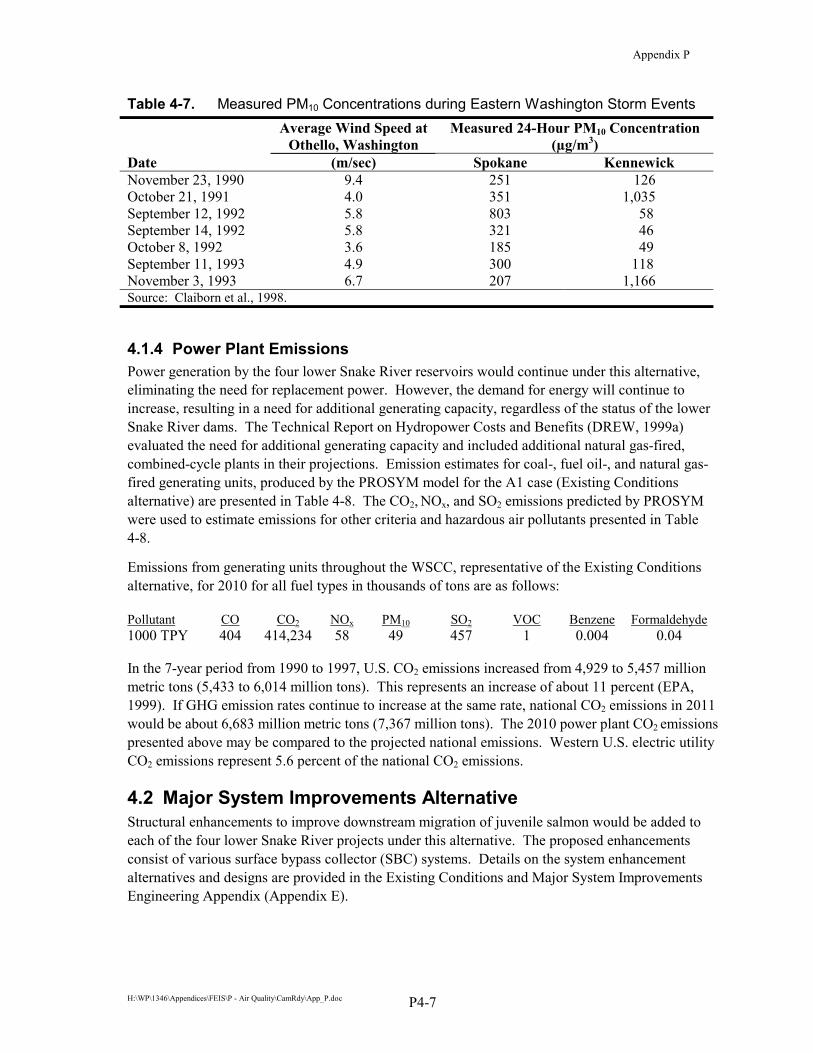
Appendix P


Table 4-7. Measured PM10 Concentrations during Eastern Washington Storm Events

Average Wind Speed at

Othello, Washington Measured 24-Hour PM10 Concentration

(µg/m3) Date (m/sec) Spokane Kennewick November 23, 1990 9.4 251 126 October 21, 1991 4.0 351 1,035 September 12, 1992 5.8 803 58 September 14, 1992 5.8 321 46 October 8, 1992 3.6 185 49 September 11, 1993 4.9 300 118 November 3, 1993 6.7 207 1,166 Source: Claiborn et al., 1998.

4.1.4 Power Plant Emissions Power generation by the four lower Snake River reservoirs would continue under this alternative, eliminating the need for replacement power. However, the demand for energy will continue to increase, resulting in a need for additional generating capacity, regardless of the status of the lower Snake River dams. The Technical Report on Hydropower Costs and Benefits (DREW, 1999a) evaluated the need for additional generating capacity and included additional natural gas-fired, combined-cycle plants in their projections. Emission estimates for coal-, fuel oil-, and natural gas-fired generating units, produced by the PROSYM model for the A1 case (Existing Conditions alternative) are presented in Table 4-8. The CO2, NOx, and SO2 emissions predicted by PROSYM were used to estimate emissions for other criteria and hazardous air pollutants presented in Table 4-8.

Emissions from generating units throughout the WSCC, representative of the Existing Conditions alternative, for 2010 for all fuel types in thousands of tons are as follows:

Pollutant CO CO2 NOx PM10 SO2 VOC Benzene Formaldehyde1000 TPY 404 414,234 58 49 457 1 0.004 0.04

In the 7-year period from 1990 to 1997, U.S. CO2 emissions increased from 4,929 to 5,457 million metric tons (5,433 to 6,014 million tons). This represents an increase of about 11 percent (EPA, 1999). If GHG emission rates continue to increase at the same rate, national CO2 emissions in 2011 would be about 6,683 million metric tons (7,367 million tons). The 2010 power plant CO2 emissions presented above may be compared to the projected national emissions. Western U.S. electric utility CO2 emissions represent 5.6 percent of the national CO2 emissions.

4.2 Major System Improvements Alternative Structural enhancements to improve downstream migration of juvenile salmon would be added to each of the four lower Snake River projects under this alternative. The proposed enhancements consist of various surface bypass collector (SBC) systems. Details on the system enhancement alternatives and designs are provided in the Existing Conditions and Major System Improvements Engineering Appendix (Appendix E).

A

ppen

dix

P

P4-8

Tabl

e 4-

8.

Pow

er G

ener

atin

g Em

issi

ons

for E

xist

ing

Con

ditio

ns A

ltern

ativ

e

Em

issi

ons (

thou

sand

s of t

ons)

G

ener

atio

n R

esou

rce

CO

C

O21/

N

Ox1/

PM

10

SO21/

V

OC

B

enze

ne

Form

alde

hyde

C

oal

Ariz

ona/

New

Mex

ico

76

77,9

52

16

19

173

0.2

0.00

130.

0002

C

anad

a 45

45

,916

8

8 75

0.

1 0.

0007

0.00

01

Nor

thw

est

12

12,1

47

2 4

40

0.03

0.

0002

0.00

003

Roc

ky M

ount

ains

11

7 11

9,82

5 24

18

16

5 0.

3 0.

0019

0.00

03

Fuel

Oil

FO #

2 0.

3 1,

142

0.04

0.

004

0.4

0.00

1 -

0.00

01

FO #

6 0.

01

37

0.00

30.

0003

0.1

0.00

01

- 0.

0000

1

Nat

ural

Gas

A

lber

ta

0.2

213

0.00

30.

0003

0.02

0.

0002

-

0.00

002

Ariz

ona/

New

Mex

ico

5 5,

000

1 0.

07

0.03

0.

04

- 0.

004

Brit

ish

Col

umbi

a 0.

4 35

8 0.

004

0.00

040.

003

0.00

02

- 0.

0000

2 Fu

ture

Com

bine

d C

ycle

87

88

,258

2

0.2

1 0.

1 -

0.01

N

orth

ern

Cal

iforn

ia

11

10,9

47

1 0.

08

0.1

0.05

-

0.00

5 PG

&E

IPPs

13

12

,961

1

0.1

1 0.

06

- 0.

006

Paci

fic N

orth

wes

t 9

8,85

6 0.

2 0.

02

0.1

0.00

9 -

0.00

1 R

ocky

Mou

ntai

ns

3 3,

200

0.5

0.04

0.

02

0.02

-

0.00

3 R

ocky

Mou

ntai

ns/C

olor

ado

2 1,

924

0.1

0.01

0.

01

0.00

6 -

0.00

1 So

uthe

rn C

alifo

rnia

13

12

,987

1

0.06

0.

1 0.

03

- 0.

004

SCE

IPPs

12

11

,758

1

0.1

3 0.

06

- 0.

007

SDG

&E

IPPs

1

753

0.1

0.01

0.

01

0.00

4 -

0.00

04

Tot

al S

yste

m E

mis

sion

s 40

4 41

4,23

4 57

.8

49.3

45

7.4

1 0.

004

0.04

1/

So

urce

: D

REW

, 199

9a.

Appendix P


4.2.1 Construction-Related Fugitive Emissions System enhancements would consist of SBC systems combined with structural modifications at each facility. The SBC structures, consisting mostly of channels, may be built from components constructed offsite, or may be built in-place. Therefore, construction-related air emissions for this alternative would be very small and would include particulate matter emissions from mixer trucks and haul roads.

For comparison of alternatives, this analysis has conservatively assumed a total of 1 MT (1.1 ton) of PM10 emissions for all four structural enhancement projects. Furthermore, construction is assumed to take place in one year.

4.2.2 Loss of Barge Transportation Barge transportation on the navigable portions of the Columbia and Snake rivers would continue with this alternative. Generally, transportation air emissions would be identical to the emission estimates presented for the Existing Conditions alternative (Section 4.1.2). With this alternative, there may be emissions increases related to operation of towboats for fish barging (Appendices A, B, and E). The increases result from loading methods and are minimal (less than 1 ton per year for all regulated air pollutants).

4.2.3 Windblown Fugitive Dust For this alternative, the four lower Snake River reservoirs would remain in their present condition. There would be no fugitive emissions from exposed reservoir sediments. Fugitive dust emissions from agricultural lands, as part the existing environment, were described in Section 4.1.3. The same emission conditions are applicable to the Major System Improvements alternative.

4.2.4 Power Plant Emissions Power generation by the four lower Snake River reservoirs would continue, eliminating the need for replacement power and associated air emissions. However, the demand for energy will continue to increase, resulting in the need for additional generating capacity. The Power System Analysis evaluated the need for additional generating capacity and included additional natural gas-fired combined-cycle power plants in their projections (DREW, 1999a). Construction of these power plants will continue for the Existing Conditions, Major System Improvements, and Dam Breaching alternatives. Emissions for the Major System Improvements alternative are very similar to those for the Existing Conditions alternative. Differences between these alternatives were not quantified.

4.3 Dam Breaching Alternative Air quality issues associated with the Dam Breaching alternative include impacts from demolition-related emissions, loss of barge transportation, windblown fugitive dust from exposed dry sediments, and emissions from thermal power plants replacing hydropower.

Air quality impacts associated with drawdown may be more extensive than presented in this section. The primary aluminum industry is an example. The availability of inexpensive electricity encouraged a primary aluminum industry in the Pacific Northwest, where alumina is electrically reduced to elemental aluminum. The process uses carbon anodes that are continuously depleted by the reaction. All or most of the carbon used in the production process is emitted as CO or CO2. In

Appendix P


1996, CO emissions equal to 26,082 metric tons (28,751 tons) were reported by an aluminum plant, located north of Spokane in Mead, Washington (EPA, 2000b). Without a source of inexpensive electricity, these sources may leave the region. Other indirect affects may include, but are not limited to, the following:

�� changes in agricultural fugitive dust emissions as farming practices shift from irrigated to dryland farming

�� changes in pesticide levels emitted along with agricultural fugitive dust emissions

�� changes in industrial emissions associated with changes in energy and transportation resources

�� changes in transportation emissions following modification of the mix of eastern Washington industries after dam breaching

�� changes in home heating practices and related emissions.

These impacts are not evaluated in this analysis.

4.3.1 Demolition-Related Fugitive Emissions Deconstruction of the four lower Snake River dams will require a number of steps, described in the Natural River Drawdown Engineering Appendix (Appendix D). The steps required to deconstruct each dam include lowering the reservoir, excavating embankments, removing cofferdams, routing the river around concrete structures, constructing levees as necessary, riprap production, and hauling and stockpiling for bank protection of existing railroad embankments. These activities would produce fugitive dust emissions. PM10 emission sources are material handling activities such as hauling, dumping, bulldozing, and grading.

4.3.1.1 Estimated Demolition Emissions Embankment and Abutment Excavation Emission Estimates

The objective of this analysis is to provide general emission estimates for the purpose of comparing the alternatives. Because many of the details, such as the number, weight, and capacity of haul trucks, length of haul roads, rate of excavation, and location of stockpiles, can only be approximated, only a preliminary analysis of fugitive emissions is possible at this time. Estimates of the equipment hours required for the project are available and are used to estimate bulldozer and grader emissions. PM10 emissions from batch dropping and hauling activities are estimated from the volume of material excavated from each facility. The methodology for the emission calculations was presented in Section 3. Excavation quantities and equipment operating hours, obtained from the Natural River Drawdown Engineering Appendix (Appendix D), are presented in Tables 3-3 and 3-4, respectively. These data were used in the emission calculations.

Fugitive PM10 emissions were calculated from emission factor expressions, default data values, operating hours, and excavation volumes presented in Section 3. It is assumed that mitigation measures (for example, watering) will achieve a 50 percent reduction in haul road emissions. The estimated PM10 emissions are presented by dam and construction activity in Table 4-9.

Appendix P


Table 4-9. Estimated Deconstruction PM10 Emissions Emissions (tons per year) Operation Ice Harbor Lower Monumental Little Goose Lower Granite Bulldozer 3.54 2.61 2.60 3.12 Hauling 150.5 183.7 67.7 63.4 Dumping 0.9 1.1 0.4 0.4 Grading 46.5 34.3 31.5 41.0 Total 201.5 221.7 102.1 108.2

Quarry Excavation Emission Estimates

Drawdown of the four lower Snake River reservoirs will require that road and railroad embankments be protected by construction of drainage structures and diversion levees. In addition, steps must be taken to repair embankments that slump following drawdown. Preliminary plans for these activities are presented in the Natural River Drawdown Engineering Appendix (Appendix D). Production of riprap for these modifications and repairs will require pre-drawdown quarry excavations that will produce fugitive dust emissions. PM10 emission sources include material handling activities such as rock screening, rock crushing, hauling, and dumping.

This analysis provides general emission estimates for quarry activities. Many details, such as the number, weight, and capacity of haul trucks, length of haul roads, rate of excavation, and volume and rate of material processed, can only be approximated at this time. PM10 emissions from screening, crushing, hauling, and dumping are all estimated from the volume of material required from each quarry. The methodology for the emission calculations was presented in Section 3. Quarried rock volumes, obtained from the Natural River Drawdown Engineering Appendix (Appendix D), are presented in Table 3-5.

Fugitive PM10 emissions were calculated from emission factor expressions, default data values, and quarried volumes presented in Section 3. It is assumed that mitigation measures (for example, watering) will achieve a 50 percent reduction in haul road emissions. Quarry activities will occur over the course of 3 years. The estimated PM10 emissions are presented in Table 4-10 by quarry and activity.

Table 4-10. Estimated Emissions from Quarry Activities Estimated Emissions (TPY) Activity Quarry 1 Quarry 2 Quarry 3 Screening rock 19 51 29 Crushing rock 0 0 0 Hauling 80 215 152 Dumping 2 4 3 Total 102 271 187

Combining the excavation and quarry emissions provides an estimate of PM10 emissions by reservoir. Emissions associated with Quarry 2 are evenly split between Lower Monumental and Little Goose. The combined emissions are as follows:

Ice Harbor Lower Monumental Little Goose Lower Granite TPY 304 357 237 295

Appendix P


4.3.1.2 Predicted Demolition Concentrations Haul road and stockpile emissions were modeled with ISCST3 and worst case meteorology. Predicted 24-hour PM10 concentrations downwind of the sources are presented on Figures 4-1 and 4-2 for the excavation and quarry haul roads, respectively. The 24-hour AAQS concentration (150 µg/m3) is indicated on the figures as a heavy contour line. The concentration appropriate for comparison to the AAQS is the maximum concentration in areas of public access. A contour plot of the predicted 24-hour concentration is presented because public restriction to the demolition site has not been established. Future modeling will indicate levels of mitigation to minimize dust emissions and areas of restricted public access. For example, it is possible to water spray the haul roads frequently to keep the road surface moist, thereby reducing fugitive emissions by about 90 percent. Alternatively, the haul roads may be paved or replaced with covered conveyors.

According to the excavation plan (Appendix D, Annex B), the demolition schedule is short (55 days). Annual average PM10 concentrations resulting from deconstruction fugitive emissions would be less than the annual AAQS (50 µg/m3).

The Wallula PM10 nonattainment area is only 18 km (11 miles) south-southeast of the Ice Harbor Dam. Although the predominant wind directions at Ice Harbor follow the orientation of the Snake River, deconstruction fugitive emissions could reach Wallula. Deconstruction emissions were modeled with 6 years of Yakima meteorological data. Predicted 24-hour PM10 concentrations at Wallula are less than the 5 �g/m3 significance level (Figure 4-3). The slight increase in concentration at about 4 km from the site represents the distance at which contributions from the various sources combine to form a maximum.

Additional analysis is required before demolition may begin. Additional data requirements include the following:

�� A detailed inventory of sources of fugitive emissions and the schedule showing when each source will be active

�� The number of trucks needed to transport the excavated material and the empty and full weight of each truck type used

�� The fugitive dust mitigation plan, including water spraying, paving, and conveyors

�� The site boundary to define areas restricted to the public

�� Site-specific variables used in the emissions calculations, including soil moisture content and road silt content

�� Site-specific meteorological data, or data sufficient to define the relationship between onsite wind conditions and a long-term database.

Appendix P


Figure 4-1. Predicted 24-Hour PM10 Concentrations from Excavations at Lower Monumental Dam

0 m 200 m 400 m 600 m

Haul Road

Stockpiles

Appendix P


Figure 4-2. Predicted 24-Hour PM10 Concentrations from Quarry Operations

0 m 200 m 400 m 600 m

Quarry

Haul Road

Barge Dump

Appendix P


Figure 4-3. Predicted 24-Hour PM10 Concentrations with Distance South of the Ice Harbor Dam

0

5

10

15

20

25

30

35

40

45

50

0 2 4 6 8 10 12 14 16 18

Downwind Distance (km)

Con

cent

ratio

n (u

g/m

3)

Appendix P


Deconstruction of the lower Snake River dams may be compared to other large demolition projects. The Elwha and Glines Canyon dams in Olympic National Park are slated for demolition. Removal of both dams would generate 200,000 yd3 of concrete, rock, and earth fill (National Park Service, 1996). Another 50,000 yd3 of concrete and compact rock fill would be used to backfill the spillway outlet channel and restore natural contours. The Lower Monumental excavation would generate 30 times more material than demolition of both the Elwha and Glines Canyon dams. The two projects are compared as follows:

Elwha and Glines Canyon Lower Monumental Excavation volume (m3) 191,000 5,716,340 Period of excavation 2 years 55 days Haul road PM10 emissions (tons) 112 171 Predicted 24-hour PM10 concentration (µg/m3) 144 150 Distance to predicted concentration (m) 100 55 and 134

4.3.2 Loss of Barge Transportation Barge transportation on the navigable portions of the Snake River would cease under the Dam Breaching alternative. Emission estimates for this alternative are compared to estimates for the Existing Conditions alternative. Emissions have been estimated from two data sources. The EWITS and Transportation Analysis studies use different methods to estimate transportation-related impacts for the Dam Breaching alternative. Methods used to estimate air emissions were presented in Section 3.

4.3.2.1 Eastern Washington Intermodal Transportation Study Transportation of wheat and barley from eastern Washington to Portland was investigated by EWITS (Lee and Casavant, 1998). Two cases were modeled by EWITS: the 1994 grain harvest with and without the availability of Snake River barge transportation. Transportation-related emissions for the Existing Conditions alternative for wheat and barley and extrapolated to other commodities were presented in Section 4.1.2. Emission estimates presented below are representative of the Dam Breaching alternative.

Grain normally shipped to Snake River ports would be trucked to elevators with rail loading facilities. Production areas away from the Snake River would truck grain to elevators adjacent to railroads. A sizable amount of grain would still be trucked directly from production areas to river ports at or below the Tri-Cities area. Elevator to river port shipments would decrease by 21 percent, while elevator to Portland rail shipments would increase by the same amount. About 28 million bushels of wheat would switch from barges to trains. About 62 percent of the barley harvest is trucked to non-Snake River ports and then barged to Portland. The volume of barley barged to Portland decreases only slightly without the Snake River.

Without the Snake River, truck traffic would be concentrated on roads that lead to and from the Tri-Cities, especially US 395. The local and rural roads east of Pasco would also receive much of the increased truck traffic.

The modeled wheat and barley ton-miles are presented in Table 3-9 for the Dam Breaching alternative. Comparison with Table 3-8 indicates that train and truck ton-miles will increase from 40 to 87 percent. Air emissions for wheat and barley transportation modes, unadjusted for return trips and other commodities, are presented in Table 4-11.

Appendix P


Table 4-11. Unadjusted Wheat and Barley Transportation-Related Emissions without the Snake River Barge Transportation Emissions (tons)

Mode Commodity CO VOC NOx PM10 SO2 Barge Wheat 38.3 12.8 281.6 6.0 50.4 Barley 4.3 1.4 31.2 0.67 5.6 Train Wheat 45.7 15.2 357.3 8.7 26.1 Barley 0.016 0.005 0.122 0.003 0.009 Truck Wheat 81.0 20.0 184.8 13.7 5.1 Barley 19.8 4.9 45.1 3.4 1.3 Total 189.1 54.3 900.1 32.5 88.5 Source: Lee and Casavant, 1998.

The emission estimates presented in Table 4-11 are for wheat and barley. Emission estimates that account for other commodities and return trips are derived in the same manner as presented in Section 4.1.2. Total transportation-related emissions are as follows:

Pollutant CO VOC NOx PM10 SO2

TPY 259 611 1,932 82 208

The change in transportation-related emissions is the difference between the emissions for the Dam Breaching and Existing Conditions alternatives and is estimated from the EWITs data as follows:

Pollutant CO VOC NOx PM10 SO2 TPY (1) 111 60 11 (48)

Trucks are used to haul grain from producers and intermediate storage locations to elevators adjacent to railroads and waterways. The movement of products over eastern Washington highways was simulated as part of EWITS GIS/GAMS modeling effort (Jessup, Ellis, and Casavant, 1997). Maps showing wheat and barley highway flows for the Dam Breaching alternative are reproduced in Annex B.

4.3.2.2 The Transportation Analysis Changes in barge, train, and truck bushel-miles are estimated as part of the Transportation Analysis. These estimates represent the change in bushel-miles required to bring the 2007 wheat and grain harvest to market following drawdown. With the Dam Breaching alternative, grain quantities normally trucked to river ports would be trucked to elevators located on rail lines or to the Tri-Cities area for barge shipment. In Idaho, the truck-miles decrease, indicating that rail-based grain elevators are closer than Lewiston. The emission factors from Lee and Casavant (1998) are used in this part of the analysis. The emission estimates are doubled to account for containers that return empty and are increased by 13 percent to include other commodities. Barge, train, and truck emissions, presented in Table 4-12, account for all commodities and vehicle return trips. The changes in total transportation-related emissions are as follows:

Pollutant CO VOC NOX PM10 SO2 TPY (14) 86 47 11 (87)

Appendix P


The NOx and SO2 emission factors are relatively large for towboats. Large decreases in barge bushel-miles translate into large decreases in NOx and SO2 emissions. The high increase in train bushel-miles, combined with the relatively high locomotive NOx emission factors, offsets the reduction in towboat NOx emissions. The truck VOC emission factor, combined with higher truck energy requirements, results in the greatest increase in VOC emissions.

Table 4-12. Change in Transportation-Related Emissions Following Dam Breaching Transportation Emissions (tons) Mode CO VOC NOx PM10 SO2

Barge (107) (36) (787) (17) (141) Train 83 31 794 51 51 Truck 10 91 40 3 3 Total (14) 86 47 11 (87)

Two data sources are used to estimate transportation-related emissions that are a consequence of the Dam Breaching alternative. The EWITS and Transportation Analysis data result in different emission estimates. The EWITS data suggest that NOx, PM10, and VOC emissions would increase, CO emissions would remain about the same, and SO2 emissions would decrease. The Transportation Analysis data indicate that NOx, PM10, and VOC emissions would increase and CO and SO2 emissions would decrease. The change in transportation-related emissions, averaged from the EWITS and Transportation Analysis results, is as follows:

Pollutant CO VOC NOx PM10 SO2 TPY (8) 98 54 11 (68)

The estimated change in transportation-related emissions may be used to estimate the change in GHG and HAP emissions. Emission factors for these pollutants, as a percent of other pollutants, were presented in Section 3.2. CO2 emissions are projected to decrease by about 700 tons per year. Benzene and formaldehyde emissions are estimated to increase by about 500 and 600 pounds, respectively.

All transportation-related emissions will continue to decline in the future as fuel efficiencies improve and as national emission standards become effective if traffic volumes remain relatively constant. Emissions standards for locomotives were scheduled to take effect in 2000. Emission standards for compression-ignition marine engines are proposed to become effective in 2004. The first phase of a proposed strategy to reduce emissions from heavy-duty vehicles will become effective in 2004. These initiatives were not considered in the emission estimates.

4.3.2.3 Estimated Vehicle Distribution Resulting from Dam Breaching The Dam Breaching alternative would change the distribution of vehicles carrying harvested grain. With drawdown, truck traffic would decrease on highways leading to river ports and would increase on roads to rail-based elevators and the Tri-Cities area. Modeling estimated the number of grain bushels on eastern Washington roads with and without drawdown (Lee and Casavant, 1998; Jessup, Ellis, and Casavant, 1997). Predicted grain quantities are used to estimate the change in the number of trucks on selected highways and are combined with WSDOT traffic counts.

Jessup, Ellis, and Casavant (1997) graphically depicted the number of bushels of grain, as a range of values, on eastern Washington roads (Annex B). The upper range, in millions of bushels, was

Appendix P


converted to truck counts at selected locations. The grain volumes and truck counts are presented in Table 4-13. The estimated number of trucks hauling grain has been doubled to account for return trips.

Table 4-13. Change in the Number of Trucks Following Dam Breaching With Snake River Without Snake River Number of Trucks Per Day

Highway Inter-section

Millions of Bushels of

Grain Total No. of

Trucks1/

Millions of Bushels of

Grain Total No. of

Trucks1/ Current

Change w/ Dam

Breaching ProjectedPercent Change

US 395 SR 26 6 6,923 59 68,083 2,480 1,003 3,483 40 SR 260 6 6,923 59 68,198 2,160 1,005 3,165 47 SR 127 SR 26 6 6,923 3 3,462 290 (57) 233 (20) SR 195 SR 272 19 21,923 7 8,077 1,920 (227) 1,693 (12) SR 26 SR 395 6 6,923 27 31,385 375 401 776 107 SR 195 3 3,462 19 21,923 575 303 878 53 SR 260 West of 395 6 6,923 2 2,308 884 (76) 808 (9) East of 395 3 3,462 2 2,308 195 (19) 176 (10) 1/ Total number of trucks per grain-harvesting season.

The greatest increase in truck counts would take place along US 395 and SR 26 just before US 395. Truck traffic along highways used to haul grain to river ports (SR 127 and SR 195) would decrease.

4.3.2.4 Traffic-Related Air Pollutant Concentrations Vehicle emissions for the US 395/SR 260 intersection were estimated by EPA’s MOBILE5 model for current traffic volumes plus 1,005 trucks per day. The EWITS modeling indicated that total wheat and barley truck traffic on SR 260 will not change appreciably with dam breaching. The SR 260 links in the highway modeling used pre-breaching emission factors. The increases in traffic on US 395, 1,005 trucks per day, are for the September through December period. The intersection was modeled using CAL3QHC and 8 years of Spokane hourly meteorological data. Increases in maximum concentrations, predicted at receptors adjacent to the roadway, represent impacts associated with the Dam Breaching alternative (Table 4-14). The predicted concentrations in Table 4-14 are also expressed as a percent of the AAQS and may be compared to the pre-breaching concentrations presented in Table 4-6. All predicted concentrations are lower than the AAQS. Following drawdown, increases in concentrations resulting from traffic emissions will be small, less than 2 percent of the AAQS.

Appendix P


Table 4-14. Predicted Highway Concentrations Following Drawdown Predicted Concentrations Period CO (ppmv) NO2 (ppmv) PM10 (µg/m3) SO2 (ppmv) Predicted Concentrations 1-hour 0.50 0.0085 3-hour 0.0077 8-hour 0.36 24-hour 7.22 0.0028 Annual 0.0178 1.95 0.0007 CO NO2 PM10 SO2 Concentration as a Percent of the AAQS 1-hour 1 3 3-hour 2 8-hour 4 24-hour 5 3 Annual 33 4 4

The model estimated the changes in emissions and ambient concentrations associated with traffic impacts resulting from drawdown. This analysis assumed the following:

�� The maximum daily traffic volumes were modeled, and it was assumed that traffic volumes do not vary throughout the year.

�� The maximum daily traffic volumes and cold weather emission factors were modeled with a full year of meteorological data to produce the average annual concentrations.

�� The traffic mix will not change from 1999 to 2010.

�� The traffic mix is based on the percent of trucks as indicated in the WSDOT traffic data.

�� Traffic lights will be added to the intersection of the on and off ramps with SR 260 before 2010.

The preliminary analysis above indicates that the increases in emissions and concentrations associated with drawdown are small.

If the Dam Breaching alternative is selected, additional analysis of traffic emissions may be required. The steps required to conduct the analysis are as follows:

�� Select several intersections that will be heavily affected by drawdown (bushel-mile modeling for the eastern Washington grain harvest conducted for the transportation economic analysis will assist with selecting intersections). Include examples of intersections affected in positive and negative manners.

�� Measure the lengths and widths of all roadway segments of the selected intersections.

�� Install roadway counters to determine total traffic volumes and periods of peak volumes.

�� Conduct a traffic survey to count vehicles by the MOBILE5 vehicle categories (light duty gasoline vehicles, light duty gasoline trucks, light duty diesel trucks, motorcycles, and so forth).

Appendix P


�� Determine the cycle time for signalized intersections or intersections that may become signalized.

�� Project the traffic volumes for an appropriate year, with and without drawdown.

�� Estimate vehicle emissions using the latest version of MOBILE5 or an equivalent mobile source emission model.

�� Model the intersections, with and without drawdown, using CAL3QHC, taking advantage of the model’s ability to vary emissions by time.

4.3.3 Windblown Fugitive Dust As drawdown proceeds, the reservoir sediments would dry and become subject to wind erosion. According to the Natural River Drawdown Engineering (Appendix D) Reservoir Revegetation Plan (Annex K), vegetation would proceed in phases:

�� Initial aerial seeding done in phases during drawdown

�� Drill seeding to revegetate areas where the initial seeding did not work

�� Manual planting of willow and cottonwood trees

�� Annual efforts to reestablish vegetation in problem or disturbed areas.

Drawdown would take place from August through October, which corresponds to the beginning of the dust storm season. Because large areas of dry sediments would be exposed to wind erosion, the total PM10 emissions may be large.

4.3.3.1 Windblown Fugitive Dust Emissions This analysis estimated PM10 emissions using EPA methods and 1984 through 1991 wind data from Pendleton, Spokane, and Yakima. For each data source, hourly average wind speeds were converted to a value representative of 2-minute speeds just above the sediment surface. A wind speed-dependent emission factor was determined for each hour when the wind speed was greater than the threshold frictional velocity. The hourly emission factors were multiplied by the area of each of the four reservoirs, a particle size multiplier, and a reduction factor to account for mitigation. The hourly emissions were added to form an annual emission estimate for each year of data, each reservoir, and each of the three data sources (Pendleton, Spokane, and Yakima). The three annual emission estimates (Pendleton, Spokane, and Yakima) were averaged. Emissions for the four reservoirs were added to form a total average PM10 emission rate.

The estimated annual PM10 emissions for the three data sources and the four reservoirs are presented in Table 4-15. The annual average PM10 emissions by reservoir (with vegetation cover) are as follows:

Ice Harbor Lower Monumental Little Goose Lower Granite TPY 1,555 1,224 1,861 1,652

The dry reservoir emission estimates overestimate the total emissions. Individual windstorms affect only a portion of the lower Snake River region, whereas the emission estimates assume that all reservoirs are subject to the same wind conditions. It is interesting to note that the threshold

Appendix P


frictional velocities of dryland soils with residue, rangelands, some dryland fallow soils, and some irrigated soils are higher than the dry reservoir sediments.

The meteorological database may be used to determine the expected number of windstorms that could produce fugitive emissions and the relative magnitude of the emissions during each storm. The frequency of emissions, in 90.7-metric ton (in 100-ton) increments, was determined for all four reservoirs by meteorological data source. The data indicate that nearly all storms produced total PM10 emissions of less than about 181 metric tons (200 tons) per event (Figure 4-4) from all four reservoirs, which is equivalent to about 5.44 kg per hectare (0.006 ton per acre).

Table 4-15. Annual Estimated Windblown PM10 Emissions Emissions (tons)

Year Ice Harbor Lower

Monumental Little Goose Lower GranitePendleton Data 1984 506 770 6831985 304 463 4111986 249 379 3361987 369 561 4981988 1,080 1,643 1,4581989 457 695 6171990 1,741 2,648 2,3511991 1,176 1,790 1,589Spokane Data 1984 1,803 1,418 2,158 1,9161985 2,017 1,587 2,415 2,1441986 2,002 1,575 2,396 2,1271987 1,807 1,422 2,163 1,9211988 3,007 2,366 3,599 3,1951989 2,857 2,248 3,420 3,0361990 3,420 2,691 4,094 3,6341991 1,627 1,280 1,948 1,729Yakima Data 1984 579 455 693 6151985 794 625 950 8441986 723 569 866 7691987 447 352 535 4751988 1,522 1,198 1,822 1,6171990 1,134 892 1,357 1,2051991 1,231 969 1,474 1,308

The results presented above are conservative. Field studies indicate that 3 hours of high wind speeds from the same direction are required to initiate windblown dust (Environalysis, 1996). Furthermore, winds producing fugitive dust in one region of the lower Snake River would not affect the entire river basin. The Revegetation Plan (Appendix D) calls for seeding sediments as the water recedes and restricting access to the dry reservoirs, thereby minimizing the amount of available erodible material. This analysis assumed that mitigation efforts would reduce emissions by 90 percent. Field studies at Owens Lake in California indicate a salt grass cover of 50 percent can

Appendix P


Figure 4-4. Frequency of Occurrence of Predicted Emissions for Individual Wind Events

reduce soil erosion and PM10 emissions by 99 percent (Great Basin Unified Air Pollution Control District, 1998). Similar reductions are expected for the dry lower Snake River reservoirs.

Rain often accompanies strong winds. This analysis did not screen out occasions of precipitation with strong winds, but it did reduce the annual emission estimates to account for the average number of days of precipitation.

The population most susceptible to windblown dust from exposed sediments would be residences along the river. Because the Snake River valley would channel the winds, residences located near river bends would be most susceptible to windblown dust.

The Owens Lake study estimated that the annual PM10 emissions are from 117,900 metric tons to 362,900 metric tons (130,000 to 400,000 tons) (Section 2.3.2). The Owens Lake emitting area is about 90.65 square kms (35 square miles), resulting in an annual emission rate of about 5.3 metric tons (5.8 tons) per acre. Once controls are in place, Owens Lake would emit about 0.2 tons per acre. Annual emissions from all four lower Snake River reservoirs, with mitigation measures in place, are estimated to be about 181.4 kg per hectare (0.2 tons per acre) on an annual basis.

4.3.3.2 Windblown Fugitive Dust Concentrations Autumn storms that produce fugitive dust from the agricultural areas of eastern Washington would also generate fugitive emissions from the dry lower Snake River reservoirs. The CP3 program modeled emissions and concentrations from several storms from 1990 to 1993. The November 1990 and October 1991 storms, modeled by CP3, are included in the meteorological database used to generate the reservoir emission estimates. Dry reservoir emissions were estimated by the methods

0102030405060708090

0 200 400 600 800 1000 1200 1400 1600 1800 2000

Emissions (tons per event)

Freq

uenc

y of

Occ

urre

nce

(per

cent

)

Pendleton Yakima Spokane

Appendix P


described in Section 3. The CP3 emissions (using two emission algorithms) and the reservoir emissions (using three data sources) are as follows:

November 23, 1990 October 21, 1991 (tons) (tons/acre) (tons) (tons/acre)

Rangeland, Dry Land, and Irrigated Land CP3 emission algorithm 11,905 0.00225 19,070 0.00473 Gillette algorithm 25,022 0.00797 186,621 0.0780 Average 18,464 0.00511 102,846 0.0414

Reservoirs Yakima winds 877 0.0259 279 0.00823 Spokane winds 3,880 0.114 606 0.0179 Pendleton winds 0 0 274 0.00808 Average 2,379 0.0468 386 0.00866

Emissions from the reservoirs are 13 and 0.4 percent of the emissions from agricultural lands for the 1990 and 1991 storms, respectively. Both of these storms moved through eastern Washington toward the northeast. The 1990 storm completely missed the Pendleton area, indicating that individual storms may influence only part of the lower Snake River reservoir system. PM10 concentration plots for three storms, reproduced from Claiborn et al. (1998), are presented in Annex C. These plots indicate that surface PM10 concentrations in the region of the reservoirs can be very large during these windstorms.

Measured Kennewick and Spokane PM10 concentrations during the 1990 and 1991 storms are available and were used by CP3 to calibrate its dispersion model. The measured 24-hour PM10 concentrations are as follows:

November 23, 1990 October 21, 1991 24-hour measured PM10 concentrations (�g/m3)

Kennewick site 126 1,035 Spokane (industrial site) - 351 Spokane (residential site) 251 267

For both storms, the duration of high wind speeds was greatest in Spokane and the winds were more intense in Spokane. Average hourly wind conditions, including the number of consecutive hours that the hourly average wind speed remained above the threshold frictional velocity, are as follows:

November 23, 1990 October 21, 1991 Yakima

Average wind speed (mph) 26 27 Maximum wind speed (mph) 32 32 Duration (hours) 20 6

Spokane Average wind speed (mph) 27 26 Maximum wind speed (mph) 35 38 Duration (hours) 82 15

Pendleton Average wind speed (mph) - 25 Maximum wind speed (mph) - 35 Duration (hours) - 7

Appendix P


By modeling PM10 concentrations resulting from fugitive dust, CP3 demonstrated that high wind speed events can produce ambient concentrations in excess of the AAQS over a large portion of eastern Washington (see Sections 3.3 and 4.1.3). PM10 concentration plots for three storms, reproduced from data developed by Claiborn et al. (1998), are presented in Annex C. The September 11 (Figure C-2) and November 3, 1993 (Figure C-3) events were major storms that produced significant ambient PM10 concentrations. The November 23, 1990 (Figure C-1) storm produced smaller but significant concentrations throughout eastern Washington.

CP3 modified the land use and soil type data, used to model the November 23 storm, to simulate emissions from the dry Snake River reservoir lake sediments. The Snake River was simulated as a straight line from Kennewick to Clarkston, Washington. When the Snake River reservoirs were modeled as the only emitting sources, the largest predicted 24-hour PM10 concentration was less than 5 �g/m3 (Figure C-4). The November 23 event was also modeled with the Snake River reservoirs and the remaining eastern Washington land cover. This plot (Figure C-5) may be compared to the contour plot for the November 23 storm modeled without the simulated Snake River.

Major storms that produce significant PM10 concentrations over large areas affect communities throughout eastern Washington. The largest population centers, such as the Tri-Cities area, may be subjected to the largest concentrations. A map showing the distribution of the eastern Washington population is presented in Annex D, and may assist in interpreting the contour plots presented in Annex C.

4.3.3.3 Windblown Hazardous Air Pollutant Concentrations

The maximum predicted PM10 concentrations resulting from windblown Snake River reservoir sediments are used to estimate the risk associated with contaminants in the sediments. To provide a degree of conservatism, the maximum ambient 24-hour PM10 concentration predicted by CP3 for Snake River sediment emissions was increased by a factor of 10 to 50 µg/m3. Assuming that 10 storm events in 1 year produce the same predicted maximum 24-hour concentrations, the resulting annual average concentration would be 1.4 µg/m3. This analysis assumed that metal and organic contaminant concentrations throughout the reservoir sediments equal the maximum measured concentrations of these pollutants (Appendix C). The resulting worst-case HAP air concentrations will be less than the risk-based ASILs (Table 4-16).

The water quality and sediment field studies and subsequent data analysis focused on identifying potential impacts associated with erosion, suspension, and transport of sediments resulting from increased river flows during drawdown. From the characterization of sediment samples, summarized in Technical Appendix C (Water Quality), manganese, dioxin and its constituents, and total DDT and its constituents were identified as contaminants of concern. Based on the analysis above, contaminated sediments are not of concern from an air quality perspective.

Appendix P


Table 4-16. Hazardous Air Pollutant Concentrations

ASIL Averaging

Uniform Soil Concentration

Needed to Produce ASIL

Maximum

Measured Soil Concentration

Air

Concentration as Percent of ASIL

Pollutant (µg/m3) Period (ppm) (ppm) (percent) Metals Arsenic 0.00023 Annual 168 7

.49 4.46

Barium 1.7 24-hour 34,000

234.8

0.69

Beryllium 0.00042 Annual 307 0.8

0.26

Cadmium 0.00056 Annual 409 0.05

0.01

Chromium 1.7 24-hour 34,000

27.1

0.08

Cobalt 0.17 24-hour 3,400

13.2

0.39

Copper 3.3 24-hour 66,000

28.6

0.04

Lead 0.5 Annual 365,000

14.9

<0.01

Manganese 0.04 24-hour 800 797.9

99.74

Mercury 0.17 24-hour 3,400

0.36

0.01

Molybdenum 17 24-hour 340,000

0.34

<0.01

Nickel 0.0021 Annual 1,533

18.5

1.21

Selenium 0.67 24-hour 13,400

2.04

0.02

Silver 0.33 24-hour 6,600

0.05

<0.01

Thallium 0.33 24-hour 6,600

0.26

<0.01

Vanadium 0.17 24-hour 3,400

58.0

1.71

Zinc 17 24-hour 340,000

71.0

0.02

Organics Dioxin 3.00E-08 Annual 0.022 0.000001 <0.01 DDT 0.01 Annual 7,300 0.0328 <0.01

Appendix P


Should a more refined analysis of HAP emissions be warranted, the following additional work would be required before the potential airborne concentrations of these pollutants can be more precisely estimated:

�� Characterize the surface concentrations of the sediments that would be subject to wind erosion [not the average of the upper 0.6096 m (2 feet) of sediment, as reported by Appendix C].

�� Determine the horizontal extent of the contaminants and the maximum and average contaminant concentrations.

�� Estimate 24-hour and annual emissions of hazardous and toxic air pollutants resulting from emissions from these sources.

�� Perform dispersion modeling for those pollutants emitted in significant quantities to determine if people living near the reservoirs are at risk.

4.3.4 Power Plant Emissions The lower Snake River dams include 3,500 MW of installed peak electrical generating capacity. Under the Dam Breaching alternative, all hydropower from the dams would be lost and would have to be replaced by a combination of energy strategies. Two options for replacing the lost hydropower have been evaluated:

�� The New Power Plants Scenario, whereby the lost hydropower would be replaced by installing new natural-gas fired power plants. For this scenario, the new power plants would result in a net increase in regional air pollutant emissions.

�� The Zero Carbon scenario, whereby the lost hydropower would be replaced by a combination of regional energy conservation and/or development of non-polluting renewable energy resources. For this scenario there would be no net increase in carbon dioxide emissions (hence the term “Zero Carbon”) or other air pollutants.

The Technical Report on Hydropower Costs and Benefits (DREW, 1999a) evaluated the costs associated with replacing power lost from the lower Snake River hydropower facilities and concluded that it would not be necessary to replace all 3,500 MW of peak hydropower capacity. The most likely scenario with dam breaching is construction of 1,550 MW of peak-generating capacity somewhere in the Pacific Northwest by 2010 by encouraging installation of combined-cycle combustion turbine power plants. The replacement power plants would not have to operate continuously at their peak rated capacity. This future replacement scenario, referred to as the New Power Plants Scenario, was used to evaluate emission impacts.

4.3.4.1 New Power Plants Scenario Description of New Thermal Power Plants

Construction of new power plants in Oregon and Washington has proceeded in the past ten years and will continue in the future regardless of the status of the lower Snake River dams. A survey of recent air discharge permit applications for power plants was completed for this study. The characteristics of 16 recently constructed or proposed power plants in Washington and Oregon are presented in Table 4-17.

Appendix P


The predominant type of thermal power plant recently added to the west coast power system has been natural gas-fired combined-cycle combustion turbine plants (DREW, 1999a). Nine of these types of power plants have been constructed in Oregon and Washington since 1991 to meet increases in power demand, and more are being planned regardless of the status of the lower Snake River dams. The Power System Analysis concluded that this type of new plant represents the most cost-effective option over a wide range of economic and environmental factors. Proposed power plants were included as sources in the power plant emission estimates for all three alternatives investigated by this analysis.

Future power generating requirements in the New Power Plants Scenario include power generators to replace hydrogeneration capacity lost if the Dam Breaching alternative is implemented. An estimate of where new power plants may be located is useful to the analysis. The hydropower study team, after reviewing studies conducted by the Northwest Power Planning Council and BPA, concluded that the following locations are the most favorable to meet power demand and transmission reliability needs:

Location Number of Combined Cycle

Plants Peak Capacity of Individual

Plants Tri-Cities area, Washington 2 250 MW Hermiston, Oregon 1 250 MW Puget Sound area, Washington 3 250 MW

Table 4-17. Summary of Recent Power Plants Constructed or to Be Constructed in the Pacific Northwest

Generic Facility Designation

Location

Year Permitted or Constructed

Number of Units

Total MW

Host

Plant 1 Chehalis, WA �1/ 2 620 Yes

Plant 2 Goldendale, WA �1/ 2 214 No

Plant 3 Boardman, OR 1995 2 504 Yes Plant 4 Bellingham, WA 1991 3 243 Yes Plant 5 Hermiston, OR 19932/ 2 476 Yes Plant 6 Hermiston, OR 19982/ 2 548 No Plant 7 Klamath, OR 1996 1 305 Yes Plant 8 Bingen, WA 1998 1 63 Yes Plant 9 Longview, WA 1996 1 96 Yes Plant 10 Anacortes, WA 1993 3 140 Yes Plant 11 Creston, WA �

1/ 4 714 No Plant 12 Vancouver, WA 1997 1 248 No Plant 13 Satsop, WA �

1/ 2 454 No Plant 14 Sumas, WA 120 Yes Plant 15 Sumas, WA �

1/ 3 507 No Plant 16 Ferndale, WA 2 245 Yes 1/ Not yet constructed. 2/ Application submitted.

In the deregulated power industry, the new power plants would be privately owned, and the actual sites would be decided by market conditions. There is a high degree of uncertainty regarding specific siting and timing of plant construction. Accordingly, these assumed plant locations and sizes are totally hypothetical.

Appendix P


Assumed Power Plant Emissions and Estimated Impacts to Local Air Quality Although the exact locations of future replacement power plants are unknown, it is assumed that the replacement power plants would be similar to those that have recently been permitted and/or constructed elsewhere in the Pacific Northwest. It is also assumed that the emissions and the ambient air quality impacts adjacent to the future replacement plants would be similar to those of the recently constructed plants. In order to evaluate the emissions and impacts to local air quality near the power plants, the air quality permits for two recently permitted power plants were reviewed:

�� The 248 MW River Road Generating Station near Vancouver, Washington, which was constructed in 1997. This plant represents the lower end of the expected size range for any future replacement plants.

�� The 660 MW Sumas 2 project at Sumas, Washington, which is currently being permitted by the Washington Energy Facility Siting Evaluation Council (EFSEC). This plant represents the upper end of the expected size range for any future replacement plants.

The expected emission controls, emission rates, and modeled ambient air quality impacts for a relatively small future replacement plant (represented by the 248 MW River Road Generating Station) are summarized in Table 4-18. The expected emissions and ambient air quality impacts for a relatively large future replacement plant (represented by the 660 MW Sumas 2 Project) are summarized in Table 4-19.

Table 4-18. Summary of Air Quality Impacts from a 248 MW Power Station Facility River Road Generating Station, Vancouver, Washington

Existing facility, began operation in 1997 Capacity 248 MW; single turbine; natural gas primary fuel; diesel fuel as backup Air quality permits Not subject to PSD or EFSEC permitting. NOC from Southwest Clean Air Agency Emission controls NOx: Low-NOx combustor with selective catalytic reduction (SCR). NOx limit =

4 ppm while burning natural gas CO: oxidation catalyst. CO limit = 6 ppm while burning natural gas

Air Pollutant Emissions and Ambient Concentrations Annual Ambient

Concentrations Caused Solely by Power Plant

Emissions (�g/m3)

24-Hour Ambient Concentrations Caused Solely by Power Plant

Emissions (�g/m3)

Pollutant

Emission Rate (tons per year)

Modeled Conc.

Allowable Limit

Modeled Conc.

Allowable Limit

NOx 99 0.2 100 – – CO 88 – – 501/ 10,000 SO2 48 0.1 52 19 262 PM10 41 0.07 50 6 150 Formaldehyde 0.45 0.0018 0.077 – – Ammonia 93 – – 0.8 100 Source: Mint Farm Generating LLC, 1999; SWAPCA, 2000. 1/ 8-hour concentration.

Appendix P


Table 4-19. Summary of Air Quality Impacts from a 660 MW Power Station Facility Sumas Energy 2 Generation Facility, Sumas, Washington

Proposed facility, currently completing permit process Capacity 2 turbines; 660 MW total; supplemental duct burners for peaking; diesel fuel as backup Air Quality Permits PSD permit from Washington EFSEC Emission Controls NOx: Low-NOx turbines with SCR. NOx limit = 2 ppm while burning natural gas

CO: oxidation catalyst. CO limit = 2 ppm while burning natural gas

Air Pollutant Emissions and Ambient Concentrations Annual Ambient

Concentrations Caused Solely by Power Plant

Emissions (�g/m3)

24-Hour Ambient

Concentrations Caused Solely by Power Plant Emissions (�g/m3)

Pollutant

Emission Rate (Tons Per Year)

Modeled Conc.

Allowable Limit

Modeled Conc. Allowable Limit

NOx 236 0.5 100 – – CO 101 – – 201/ 10,000 SO2 45 0.1 52 14 262 PM10 223 0.5 50 10 150 Formaldehyde 0.1 0.0008 0.077 – – Ammonia 139 – – 4 100 Sulfuric Acid Mist 8 – – 3.0 3.3 CO2 2.4 million – – – –

Acid Deposition and Visibility Impacts at North Cascades National Park

Environmental Impact

Impact Caused by Power Plant

Emissions Recommended

Limit Nitrogen deposition at North Cascades National Park (kg/hectare/yr) 0.0014 0.005 – 0.10 Visibility impact at North Cascades National Park while firing

primary natural gas (increase in 24-hour b-ext) 2.5% 5%

Visibility impact at North Cascades National Park while firing backup oil fuel (increase in 24-hour b-ext)

7.5% 5%

Source: Sumas Energy 2 Generating Facility, 2000; EFSEC, 2000. 1/ 8-hour concentration.

Comparison of the air quality impacts for those two actual plants shows the following:

�� Permitting Requirements – The River Road Generating Station required only a conventional NOC air quality permit from the local air quality agency because its rated capacity is less than 250 MW (the threshold for permitting by EFSEC) and it emits less than 100 tons per year of any single pollutant (the threshold for PSD permitting). The relatively large Sumas 2 Project requires a PSD permit issued by EFSEC.

�� Emission Controls – Both plants use the same emission controls. NOx is controlled by Selective Catalytic Reduction (SCR) with ammonia injection. CO, VOC, and HAPs are controlled by an oxidation catalyst. SO2 (emitted mainly from backup oil combustion) is controlled by use of low-sulfur oil and restrictions on the annual usage of fuel oil.

�� Ambient Air Quality Impacts – The worst-case local ambient concentrations of criteria pollutants and toxic air pollutants adjacent to both plants are well below Washington’s allowable limits. The air quality impacts at the Sumas 2 project were less than the allowable PSD Class II increments. The local air quality impacts were estimated using EPA’s

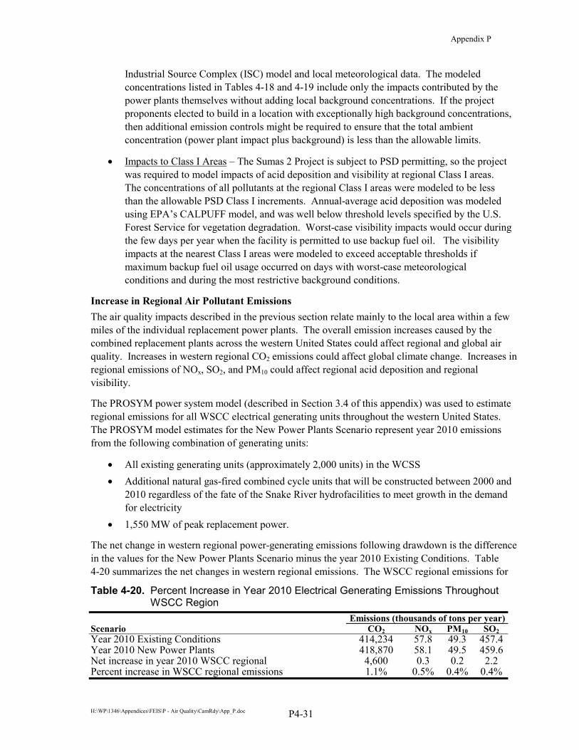
Appendix P


Industrial Source Complex (ISC) model and local meteorological data. The modeled concentrations listed in Tables 4-18 and 4-19 include only the impacts contributed by the power plants themselves without adding local background concentrations. If the project proponents elected to build in a location with exceptionally high background concentrations, then additional emission controls might be required to ensure that the total ambient concentration (power plant impact plus background) is less than the allowable limits.

�� Impacts to Class I Areas – The Sumas 2 Project is subject to PSD permitting, so the project was required to model impacts of acid deposition and visibility at regional Class I areas. The concentrations of all pollutants at the regional Class I areas were modeled to be less than the allowable PSD Class I increments. Annual-average acid deposition was modeled using EPA’s CALPUFF model, and was well below threshold levels specified by the U.S. Forest Service for vegetation degradation. Worst-case visibility impacts would occur during the few days per year when the facility is permitted to use backup fuel oil. The visibility impacts at the nearest Class I areas were modeled to exceed acceptable thresholds if maximum backup fuel oil usage occurred on days with worst-case meteorological conditions and during the most restrictive background conditions.

Increase in Regional Air Pollutant Emissions The air quality impacts described in the previous section relate mainly to the local area within a few miles of the individual replacement power plants. The overall emission increases caused by the combined replacement plants across the western United States could affect regional and global air quality. Increases in western regional CO2 emissions could affect global climate change. Increases in regional emissions of NOx, SO2, and PM10 could affect regional acid deposition and regional visibility.

The PROSYM power system model (described in Section 3.4 of this appendix) was used to estimate regional emissions for all WSCC electrical generating units throughout the western United States. The PROSYM model estimates for the New Power Plants Scenario represent year 2010 emissions from the following combination of generating units:

�� All existing generating units (approximately 2,000 units) in the WCSS �� Additional natural gas-fired combined cycle units that will be constructed between 2000 and

2010 regardless of the fate of the Snake River hydrofacilities to meet growth in the demand for electricity

�� 1,550 MW of peak replacement power.

The net change in western regional power-generating emissions following drawdown is the difference in the values for the New Power Plants Scenario minus the year 2010 Existing Conditions. Table 4-20 summarizes the net changes in western regional emissions. The WSCC regional emissions for

Table 4-20. Percent Increase in Year 2010 Electrical Generating Emissions Throughout WSCC Region

Emissions (thousands of tons per year)Scenario CO2 NOx PM10 SO2 Year 2010 Existing Conditions 414,234 57.8 49.3 457.4Year 2010 New Power Plants 418,870 58.1 49.5 459.6Net increase in year 2010 WSCC regional 4,600 0.3 0.2 2.2 Percent increase in WSCC regional emissions 1.1% 0.5% 0.4% 0.4%

Appendix P


the Year 2010 Existing Conditions were discussed in Section 4.1.4 of this appendix. The Year 2010 WSCC emissions for the New Power Plants Scenario are itemized in Table 4-21.

Table 4-20 indicates that WSCC regional CO2 emissions would increase by 4.2 million metric tons per year (4,600,000 tons/year) compared to the Year 2010 Existing Conditions. NOx emissions would increase by 272 metric tons per year (300 tons/year). PM10 emissions would increase by 181 metric tons per year (200 tons/year).

Impacts to Greenhouse Gas Emissions and Global Warming

Replacement power plants constructed in the western United States would increase regional emissions of CO2 and could affect global warming. Because CO2 emissions from each power plant cause global impacts rather than local impacts, the CO2 emissions from the combined power plants are best compared to regional and nationwide CO2 emissions.

In the 8-year period from 1990 to 1998, nationwide United States CO2 emissions increased from 9,806 million metric tons to 10,932 million metric tons (10,809 to 12,050 million tons), an increase of about 11 percent. If GHG emission rates continue to increase at the same rate, national CO2 emissions in 2010 will be about 12,519 million metric tons (13,800 million tons). For the planning period of 1990-2010, this represents a nationwide CO2 emission increase of 2,713 million metric tons (2,991 million tons). For comparison, the 1,500 MW capacity of replacement power plants would increase CO2 emissions in the WSCC region by 4.2 million metric tons per year (4.6 million tons/year). Based on these forecasted emission estimates, the relative impact of the New Power Plants Scenario can be summarized as follows:

�� In the year 2010, the total WSCC electrical generating CO2 emissions are forecasted to be about 3.0 percent of the nationwide total emissions.

�� The net CO2 emission increase caused by the 1,550 MW capacity of new replacement power plants would be about 1.1 percent of the WSCC western regional emissions.

�� The net CO2 emission increase caused by the 1,550 MW capacity of new replacement power plants would be about 0.14 percent of the nationwide CO2 increase during the period 1990 to 2010.

4.3.4.2 Zero Carbon Scenario As described in Section 4.3.4.1, replacement power plants for the New Power Plants scenario would increase CO2 emissions from western regional electric utilities by 4.2 million tons per year compared to the Existing Conditions alternative. This predicted CO2 emission increase is roughly 1 percent of the total for all combined electrical generating units within the WSCC region.

An emission increase of that magnitude is counter to the United States Climate Change Action Plan, which includes a goal to reduce nationwide CO2 emissions to year 1990 levels. Therefore, the U.S. Army Corps of Engineers, Northwest Power Planning Council (NWPPC), and Natural Resources Defense Council (NRDC) have evaluated the feasibility of an alternative to offset the lost hydropower from the lower Snake River dams without installing any new natural-gas fired power plants. Under this alternative the CO2 emissions for the Dam Breaching alternative would be the same as for the Existing Conditions alternative. This alternative is therefore designated the Zero Carbon Scenario.

App

endi

x P

P4-33

Tabl

e 4-

21.

Year

201

0 W

SCC

Reg

iona

l Em

issi

ons

for N

ew P

ower

Pla

nts

Scen

ario

Yea

r 20

10 E

mis

sion

s Thr

ough

out W

SCC

(tho

usan

ds o

f ton

s per

yea

r)

Gen

erat

ion

Res

ourc

e C

O

CO

21/

NO

x1/

PM10

SO

21/

VO

C

Ben

zene

Fo

rmal

dehy

de

Coa

l

A

rizon

a/N

ew M

exic

o 76

77

,957

16

19

17

3 0.

2 0.

001

0.00

02

Can

ada

45

46,0

60

8 8

75

0.1

0.00

07

0.00

01

Nor

thw

est

12

12,5

22

2 4

41

0.04

0.

0002

0.

0000

4 R

ocky

Mou

ntai

ns

117

120,

144

24

18

165

0.3

0.00

2 0.

0003

Fuel

Oil

FO #

2 0.

3 1,

098

0.04

0.

004

0.4

0.00

1 -

0.00

008

FO #

6 0.

01

36

0.00

3 0.

0003

0.

1 0.

0000

7 -

0.00

0006

Nat

ural

Gas

A

lber

ta

0.2

190

0.00

2 0.

0002

0.

02

0.00

01

- 0.

0000

1 A

rizon

a/N

ew M

exic

o 5

4,84

4 0.

7 0.

07

0.03

0.

04

- 0.

004

Brit

ish

Col

umbi

a 0.

3 30

4 0.

004

0.00

03

0.00

3 0.

0002

-

0.00

002

Futu

re c

ombi

ned

cycl

e 91

92

,713

2

0.2

0.6

0.1

- 0.

01

Nor

ther

n C

alifo

rnia

10

10

,583

0.

8 0.

08

0.07

0.

04

- 0.

005

PG&

E IP

Ps

13

12,7

92

1 0.

1 1

0.06

-

0.00

6 Pa

cific

Nor

thw

est

9 8,

926

0.2

0.02

0.

06

0.00

9 -

0.00

1 R

ocky

Mou

ntai

ns

3 3,

154

0.4

0.04

0.

02

0.02

-

0.00

3 R

ocky

Mou

ntai

ns/C

olor

ado

2 1,

905

0.1

0.01

0.

01

0.00

6 -

0.00

06

Sout

hern

Cal

iforn

ia

12

12,7

10

0.6

0.06

0.

09

0.03

-

0.00

4 SC

E IP

Ps

12

11,7

28

1 0.

1 3

0.06

-

0.00

7 SD

G&

E IP

Ps

0.7

752

0.07

0.

006

0.00

5 0.

004

- 0.

0004

T

otal

Sys

tem

Em

issi

ons

408

418,

870

58.1

49

.5

459.

6 1

0.00

4 0.

04

1/

Sour

ce:

DR

EW, 1

999a

.

Appendix P


The engineering and economic details of the Zero Carbon scenario are described in Section 5.9.4 of the EIS. The PROSYM power model was used to determine the amount of non-polluting energy conservation that would be required to offset the emissions from new thermal power plants. Under the Zero Carbon Scenario, the 1,550 MW of lost hydropower would be offset by a combination of energy conservation measures and clean, renewable generation measures. The actual net loss of hydropower production from dam breaching would be 940 aMW, according to a report by the Natural Resources Defense Council (2000). This evaluation considers impacts from an operational base case from increased spill, increased fish barge transport, and reoptimizing the electricity generating system once the dams are removed. The Natural Resources Defense Council study assumes that 1,091 aMW of power (75 percent from conservation and the remaining amount from non-hydro renewable energy sources such as wind and solar) would be required to replace the lost 940 aMW of hydropower without any increase in carbon emissions from the base case due to timing considerations for reduced comsumption. A concurrent analysis was conducted by the Corps with slightly different assumptions and very similar conclusions. In the Corps analysis, approximately 820 aMW of thermal power would have to be replaced by conservation for substantially no net increase in carbon emissions in 2010 compared to the base case of leaving the dams in place. Because the load curves of lower Snake River hydropower differ from the load curves for available conservation, a total of 1,150 aMW of conservation would have to be enacted to offset the 820 aMW of lost hydropower. The 1,150 aMW of new energy conservation would represent a decrease of 5.3 percent of the forecasted load in the WSCC region for the year 2010.

It is uncertain whether 1,150 aMW of new energy conservation is readily available within the region. In addition, there is uncertainty regarding the relative costs of 1,150 aMW of new conservation compared to the cost of 820 aMW of new thermal power plants. Based on published reports (NWPPC, 1996; NRDC, 2000), as of 1996 there were an estimated 1,535 aMW of low-cost energy conservation available to BPA (“low-cost” conservation is defined as costing less than 3 cents per kw-hr). A summary of the identified conservation measures is given in Table 4-22. However, voluntary measures have already consumed about 500 aMW of available low-cost conservation since 1996. Therefore, it is possible that the Zero Carbon Scenario would require enactment of additional resources beyond low-cost conservation. Such additional measures could include pursuing high-cost energy conservation and subsidizing development of non-polluting renewable energy systems such as wind power.

Table 4-22. Achievable Conservation for Zero Carbon Scenario End Use Sector Achievable Conservation (aMW)

Freezers 15 Refrigerators 45 Water heating 335 Residential lighting 30 New residential space heating 140 Existing residential space heating 25 New commercial 230 Existing commercial 95 Commercial renovation/remodel 50 New non-aluminum industrial 225 Existing non-aluminum industrial 335 Direct service aluminum industrial Not estimated Irrigated agriculture 10 Total 1,535

Appendix P


5. Comparison of Alternatives This section compares the atmospheric emissions estimated for the Existing Conditions, Major System Improvements, and Dam Breaching alternatives, and includes a brief discussion of potential mitigation measures, cumulative effects, and unavoidable adverse effects.

This analysis estimated criteria air pollutants and TAP emissions for the Existing Conditions, Major System Improvements, and Dam Breaching alternatives. The air quality issues related to the Lower Snake River Juvenile Salmon Migration Feasibility Study are:

�� Fugitive dust emissions resulting from deconstruction of the dams

�� A change in the quantity and distribution of vehicle emissions as commodities are shifted from barge to truck and rail

�� Fugitive dust emissions resulting from dry exposed lake sediments during high wind speed events

�� Atmospheric emissions associated with replacement power generation by thermal power plants.

Estimated air quality impacts are presented below by alternative. Cumulative effects, mitigation measures, unavoidable adverse effects, and incomplete information are also discussed below.

5.1 Summary of Emissions by Alternative Emissions estimated in Section 4 are summarized in Table 5-1. Emission increases above those estimated for the Existing Conditions alternative are presented in Table 5-1 for the Major System Improvements and Dam Breaching alternatives. Transportation-related emissions are an average of the estimates produced from the EWITS and Transportation Analysis data. The Transportation Analysis estimated the change in emissions following drawdown. The Dam Breaching transportation-related emissions are indeterminant. Worst-case ambient concentrations, as a percent of the AAQS, are presented for representative Existing Conditions and Dam Breaching emissions sources in Table 5-2. The data in Table 5-2 represent the maximum ambient air quality concentrations predicted for any receptor as part of the evaluation of that pathway. As indicated by Table 5-2, emissions associated with the EIS alternatives result in ambient concentrations less than the AAQS. PM10 concentrations associated with deconstruction activities will be less than the AAQS once public access restrictions are defined.

5.2 Existing Conditions Alternative 5.2.1 Direct and Indirect Effects No emission increases are estimated for the Existing Conditions, which represents current conditions projected to 2010. Therefore, this alternative would have no direct or indirect air quality effects. Under this alternative, Snake River barge traffic would continue and new power plants would continue to be built as power demand increases. Emissions from these new plants have been factored into the analysis.

A

ppen

dix

P

P5-2

Tabl

e 5-

1.

Sum

mar

y of

Em

issi

ons

in T

ons

E

mis

sion

s (to

ns p

er y

ear)

CO

C

O2

NO

x PM

10

SO2

VO

C

Ben

zene

Fo

rmal

dehy

deE

xist

ing

Con

ditio

ns

Dem

oliti

on

Tran

spor

tatio

n 23

5 20

,680

1,

705

52

266

285

1 1

Win

dblo

wn

Dus

t

Po

wer

Gen

erat

ion

403,

624

414,

233,

886

57,7

57

49,2

67

457,

383

1,13

2 4

45

Tot

al

403,

859

414,

254,

566

59,4

62

49,3

19

457,

649

1,41

7 5

46

Maj

or S

yste

m Im

prov

emen

ts

Con

stru

ctio

n

Tran

spor

tatio

n 23

5 20

,680

1,

705

52

266

285

1 1

Win

dblo

wn

Dus

t

Po

wer

Gen

erat

ion

403,

624

414,

233,

886

57,7

57

49,2

67

457,

383

1,13

2 4

45

Tot

al

403,

859

414,

254,

566

59,4

62

49,3

20

457,

649

1,41

7 5

46

Cha

nge

from

Exi

stin

g Sy

stem

0

0 0

1 0

0 0

0 N

ew P

ower

Pla

nts S

cena

rio

Dem

oliti

on

1,

193

Tr

ansp

orta

tion

227

19,9

76

1,75

9 63

19

8 38

3 1

1 W

indb

low

n D

ust

6,

292

Pow

er G

ener

atio

n 40

7,75

8 41

8,87

0,00

0 58

,100

49

,463

45

9,60

0 1,

134

4 45

T

otal

40

7,98

5 41

8,88

9,97

6 59

,859

57

,011

45

9,79

8 1,

517

5 46

C

hang

e fr

om E

xist

ing

Syst

em

4,12

6 4,

635,

410

397

7,69

2 2,

149

101

0 0

Zero

Car

bon

Scen

ario

D

emol

ition

1,19

3 Tr

ansp

orta

tion

227

19,9

76

1,75

9 63

19

8 38

3 1

1 W

indb

low

n D

ust

6,

292

Pow

er G

ener

atio

n 40

3,62

4 41

4,23

3,88

6 57

,757

49

,267

45

7,38

3 1,

132

4 45

T

otal

40

3,85

1 41

4,25

3,86

2 59

,516

56

,815

45

7,58

1 1,

515

5 46

C

hang

e fr

om E

xist

ing

Syst

em

(8)

(704

) 54

7,

496

(68)

98

0

0

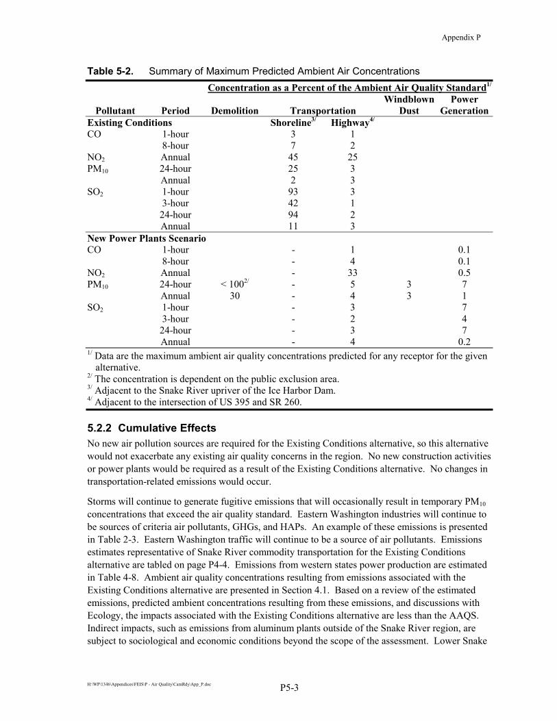
Appendix P


Table 5-2. Summary of Maximum Predicted Ambient Air Concentrations Concentration as a Percent of the Ambient Air Quality Standard1/

Pollutant Period Demolition Transportation Windblown

Dust Power

GenerationExisting Conditions Shoreline3/ Highway4/ CO 1-hour 3 1 8-hour 7 2 NO2 Annual 45 25 PM10 24-hour 25 3 Annual 2 3 SO2 1-hour 93 3 3-hour 42 1 24-hour 94 2 Annual 11 3 New Power Plants Scenario CO 1-hour - 1 0.1 8-hour - 4 0.1 NO2 Annual - 33 0.5 PM10 24-hour < 1002/ - 5 3 7 Annual 30 - 4 3 1 SO2 1-hour - 3 7 3-hour - 2 4 24-hour - 3 7 Annual - 4 0.2 1/ Data are the maximum ambient air quality concentrations predicted for any receptor for the given

alternative. 2/ The concentration is dependent on the public exclusion area. 3/ Adjacent to the Snake River upriver of the Ice Harbor Dam. 4/ Adjacent to the intersection of US 395 and SR 260.

5.2.2 Cumulative Effects No new air pollution sources are required for the Existing Conditions alternative, so this alternative would not exacerbate any existing air quality concerns in the region. No new construction activities or power plants would be required as a result of the Existing Conditions alternative. No changes in transportation-related emissions would occur.

Storms will continue to generate fugitive emissions that will occasionally result in temporary PM10 concentrations that exceed the air quality standard. Eastern Washington industries will continue to be sources of criteria air pollutants, GHGs, and HAPs. An example of these emissions is presented in Table 2-3. Eastern Washington traffic will continue to be a source of air pollutants. Emissions estimates representative of Snake River commodity transportation for the Existing Conditions alternative are tabled on page P4-4. Emissions from western states power production are estimated in Table 4-8. Ambient air quality concentrations resulting from emissions associated with the Existing Conditions alternative are presented in Section 4.1. Based on a review of the estimated emissions, predicted ambient concentrations resulting from these emissions, and discussions with Ecology, the impacts associated with the Existing Conditions alternative are less than the AAQS. Indirect impacts, such as emissions from aluminum plants outside of the Snake River region, are subject to sociological and economic conditions beyond the scope of the assessment. Lower Snake

Appendix P


River regional emissions associated with the four air quality issues investigated in this assessment are tabled with a comparison of other alternative-specific emissions in Table 5.1.

5.2.3 Mitigation Measures No mitigation measures are required for the Existing Conditions alternative. No new construction activities or power plants would be required as a result of the Existing Conditions alternative. No changes in transportation-related emissions would occur.

5.2.4 Unavoidable Adverse Effects The Existing Conditions alternative would not cause any adverse air quality impacts.

5.2.5 Incomplete Information No additional information related to air quality is required for the Existing Conditions alternative.

5.3 Major System Improvements Alternative 5.3.1 Direct and Indirect Effects Minor construction-related emission increases are anticipated for the Major System Improvements alternative. Therefore, only minor direct or indirect air quality effects would result. As with the Existing Conditions alternative, Snake River barge traffic would continue, and no new power plants would be required as a result of actions taken at the Snake River dams. Emission estimates for the Major System Improvements alternative are identical to those of the Existing Conditions alternative.

5.3.2 Cumulative Effects Cumulative effects for the Major System Improvements alternative are the same as for the Existing Conditions alternative.

Storms will continue to generate fugitive emissions that will occasionally result in temporary PM10 concentrations that exceed the air quality standard. Eastern Washington industries will continue to be sources of criteria air pollutants, GHGs, and HAPs. An example of these emissions is presented in Table 2-3. Eastern Washington traffic will continue to be a source of air pollutants. Emissions estimates representative of Snake River commodity transportation for the Major Systems Improvements alternative are tabled on page P4-4. Emissions from western states power production are estimated in Table 4-8. Ambient air quality concentrations resulting from emissions associated with the Major Systems Improvements alternative are presented in Section 4.1. Based on a review of the estimated emissions, predicted ambient concentrations resulting from these emissions, and discussions with Ecology, the impacts associated with the Major Systems Improvements alternative are less than the AAQS. Indirect impacts, such as emissions from aluminum plants outside of the Snake River region, are subject to sociological and economic conditions beyond the scope of the assessment, although traditional low-cost hydropower is critical to their continued operations. Lower Snake River regional emissions associated with the four air quality issues investigated in this assessment are tabled with a comparison of other alternative-specific emissions in Table 5-1.

Appendix P


5.3.3 Mitigation Measures No mitigation measures related to air quality are required for the Major System Improvements alternative.

5.3.4 Unavoidable Adverse Effects The Major System Improvements alternative would not cause any adverse air quality impacts.

5.3.5 Incomplete Information No additional information related to air quality is required for the Major System Improvements alternative.

5.4 Dam Breaching Alternative 5.4.1 Direct and Indirect Effects As listed in Table 5-1, the Dam Breaching alternative would result in increased air pollutant emissions compared to the Existing Conditions alternative. This pathway would result in fugitive emissions (PM10) from demolition, transportation emissions associated with the loss of barge transportation (criteria air pollutants), fugitive dust from exposed reservoir sediments, and emissions associated with replacement power generation (criteria air pollutants, HAPs, and GHGs). The transportation-related emission estimates do not consider tire and brake emissions.

However, as listed in Table 5-2, the increased emissions from project-related activities would not cause any ambient air pollutant concentrations greater than the AAQS. In addition, the project-related emissions would not adversely affect any nearby nonattainment areas.

Increased CO2 emissions caused by the replacement power plants would account for about one percent of the western regional emissions from WSCC’s power generating units.

5.4.2 Cumulative Effects Storms will continue to generate fugitive emissions that will occasionally result in temporary PM10 concentrations that exceed the air quality standard. Eastern Washington industries will continue to be sources of criteria air pollutants, GHGs, and HAPs. An example of these emissions is presented in Table 2-3. Demolition-related emission estimates are tabulated on page P4-11. Eastern Washington traffic will continue to be a source of air pollutants. The change in emissions representative of Snake River commodity transportation for the Dam Breaching alternative are tabled on page P4-17. Emissions from western states power production are estimated in Table 4-21. Ambient air quality concentrations resulting from emissions associated with the Dam Breaching alternative are presented in Section 4.3. Based on a review of the estimated emissions, predicted ambient concentrations resulting from these emissions, and discussions with Ecology, the impacts associated with the Dam Breaching alternative are less than the AAQS. Indirect impacts, such as emissions from aluminum plants outside of the Snake River region, are subject to sociological and economic conditions beyond the scope of the assessment. Lower Snake River regional emissions associated with the four air quality issues investigated in this assessment are tabled with a comparison of other alternative-specific emissions in Table 5-1.

Appendix P


5.4.2.1 Deconstruction Fugitive Dust According to Appendix D, drawdown may take place during the eastern Washington storm season (September through November). Should a high wind speed event occur during deconstruction, lake sediments and excavated material would be available for erosion. The fugitive dust problem would be exacerbated if all four dams were removed at once.

5.4.2.2 Transportation-Related Emissions Increased tailpipe emissions from haul trucks that would replace the existing barge system would probably not cause any significant cumulative impacts. Existing background concentrations of NOx and CO (the primary tailpipe emissions) along the expected haul truck routes are much lower than the AAQS. The increased emissions would not significantly increase the background concentrations.

5.4.2.3 Windblown Fugitive Dust The Columbia Plateau region already experiences high PM10 concentrations, and Ecology indicates that in the future, portions of the region could be designated as nonattainment areas. Construction-related fugitive emissions could be effectively controlled, so temporary impacts during dam deconstruction would probably not exacerbate regional problems. However, long-term windblown dust from the dry lake beds could be difficult to control. These emissions could exacerbate regional PM10 problems that already occur during occasional high wind events.

5.4.2.4 Power Plant Emissions NOx and CO emissions from replacement power plants would not exacerbate any existing ambient air quality concerns, even if some of the plants were constructed in urban areas. State air quality regulations would require the power plant emissions to be stringently controlled. Local air quality agency staff have indicated that the increased emissions from any of the replacement plants would not significantly affect their future ability to satisfy the AAQS. CO2 emissions from replacement power plants could exacerbate future difficulties in reducing national and regional emissions down to historical 1990 levels, as recommended by the United States Climate Change Action Plan.

5.4.3 Mitigation Measures

5.4.3.1 Deconstruction Fugitive Dust Deconstruction of the dams would incorporate standard construction practices to suppress fugitive dust, such as spraying haul roads with water. Some of the dam core material would be saturated with water, reducing the potential for fugitive dust emissions. Deconstruction of the individual Snake River dams would most likely not take place in the same year.

5.4.3.2 Transportation-Related Emissions No special mitigation is warranted for highway trucks that would replace the existing barge system. Vehicles will continue to experience efficiency improvements and associated reductions in emissions.

Appendix P


5.4.3.3 Windblown Fugitive Dust Stringent control of windblown dust from the dry lake beds would be required. Appendix D, Natural River Drawdown Engineering, calls for phased revegetation as the water recedes. In addition, access to the dry lakebed would be restricted, further reducing the availability of erodible material. The analysis assumes that dry sediments are disturbed between high wind-speed events, thereby providing additional erodible material. The emission estimates for windblown dust described in this appendix are believed to be conservatively high.

5.4.3.4 Power Plant Emissions New power plants would have to install stringent emission controls mandated by Best Available Control Technology. If such emission controls are required, then the replacement plants would not cause significant impacts to ambient air quality. Carbon dioxide emissions from replacement power plants could be minimized by a combination of mitigations. Any replacement plants could be required to achieve a CO2 emission limit equivalent to Oregon’s standards and pay emission fees to fund regional CO2 reduction efforts. The Zero Carbon Scenario could be used, whereby hydropower lost from the Snake River dams would be replaced by a combination of energy conservation and non-polluting renewable energy.

5.4.4 Unavoidable Adverse Effects If the lower Snake River dams are breached, deconstruction, transportation, windblown dust, and power plant emissions would take place.

5.4.4.1 Deconstruction Fugitive Dust Fugitive dust emissions during dam deconstruction can be controlled so the ambient impacts are less than the allowable AAQS. Breaching of the dams would resemble a large construction project. Deconstruction of the dams would probably take several years and/or would be staged, resulting in lower emissions per year.

5.4.4.2 Transportation-Related Emissions Tailpipe emissions from haul trucks that would replace existing barges would not significantly affect ambient air quality. Emissions of CO, NOx and SO2 would decline by 1 to 30 percent. Emissions of PM10 and VOCs would increase by 20 to 30 percent above the Existing Conditions alternative emissions. Truck traffic on US 395 would increase by as many as 200 trucks per day (in both directions) during the period of grain hauling. The number of trucks on US 195 at SR 272 would decrease by more than 1,000 trucks per day.

5.4.4.3 Windblown Fugitive Dust Storms would generate fugitive emissions from the dry lake beds until the vegetation cover becomes established. These new emissions could exacerbate existing problems with regional windblown dust. Emissions from the dry reservoirs would be between 0.4 and 13 percent of the total emissions from eastern Washington agricultural areas during individual windstorms. The resulting ambient concentrations may be a problem, especially if the surface sediments are contaminated.

Appendix P


5.4.4.4 Power Plant Emissions Emissions from each individual power plant would cause localized increases in ambient concentrations, but the local increases would probably be insignificant compared to the AAQS. Western regional emissions of criteria air pollutants, HAPs, and GHGs would increase by 1 percent or less above the Existing Conditions alternative emissions. CO2 emissions from replacement power plants would be 0.14 percent of the nationwide increase in emissions during the planning period 1990-2010.

5.4.5 Areas of Possible Future Study The emission calculations used available data and reasonable values for preliminary information. Because of information gaps, the emissions are considered estimates and are intended for comparison of the alternatives. Furthermore, the estimates are used to predict ambient concentrations resulting from deconstruction, transportation, fugitive dust, and power-related emissions. Additional data and studies are necessary to characterize, in detail, the impacts associated with drawdown. Site specific data are listed below.

5.4.5.1 Deconstruction Fugitive Dust Construction schedules, moisture and silt content of excavated material and haul roads, areas and volumes of stockpiles, and length of haul roads are required for deconstruction emission estimates. Predicting ambient concentrations resulting from fugitive emissions requires the distances to critical receptors and may require on-site meteorological data and background PM10 concentrations. These refined emissions estimates would be prepared as part of the environmental evaluations for each individual dam.

5.4.5.2 Transportation-Related Emissions The analysis conducted for this appendix indicated that transportation-related emissions will not produce an air quality problem. However, increasing traffic congestion may require modification to critical intersections (addition of extra lanes and signalization), regardless of the status of the Snake River dams. To optimize traffic flow and minimize vehicle emissions, traffic and intersection modeling, similar to analysis presented in this appendix, may be required.

5.4.5.3 Windblown Fugitive Dust Additional maps of the reservoir topography, surface sediment grain-size analysis, the distribution of fine material within the reservoirs, onsite wind conditions, background concentrations, and the location of sensitive receptors are required to characterize windblown dust. The location, concentration, and extent of contaminated surface sediment are required to characterize hazardous air pollutant emissions. If the regions that include the reservoirs are declared nonattainment areas, post drawdown ambient PM10 monitoring adjacent to the dry reservoirs may be required. A modeling analysis, similar to the impact analysis, may be necessary to properly site the monitoring station.

5.4.5.4 Power Plant Emissions Emissions of criteria and hazardous air pollutants from power plants and ambient concentrations resulting from power plant emissions, including cumulative impacts and air quality-related values in protected areas, will be addressed in permit application documents after specific designs for the plants have been developed.

Appendix P


6. Literature Cited Benson, P.E. 1979. CALINE3 – A Versatile Dispersion Model for Predicting Air Pollutant Levels

Near Highways and Arterial Streets. Abridged. California Department of Transportation. November 1979.

Bonneville Power Administration, U.S. Army Corps of Engineers, and Bureau of Reclamation. 1995. Columbia River System Operation Review, Final Environmental Impact Statement: Appendix B – Air Quality. November 1995.

Bureau of Reclamation. 1989. Draft Environmental Impact Statement, Continued Development of the Columbia Basin Project, Washington. DES89-19. U.S. Department of the Interior, Bureau of Reclamation, Pacific Northwest Region. Boise, Idaho.

Claiborn, C., B. Lamb, A. Miller, J. Beseda, B. Clode, J. Vaughan, L. Kang, and C. Newvine. 1998. Regional Measurements and Modeling of Windblown Agricultural Dust: The Columbia Plateau PM10 Program. Journal of Geophysical Research. 103(D16):19,753-19,767.

Corps (U.S. Army Corps of Engineers, Walla Walla District). 1999. Regional Precipitation Map, Preliminary Lower Snake River Juvenile Salmon Migration Feasibility Study. Plotted 12 February 1999. Source: Climatogical Handbook, Columbia Basin States, Precipitation, June 1969.

DREW (Drawdown Regional Economic Workshop Hydropower Impact Team). 1999a. Lower Snake River Juvenile Salmon Migration Feasibility Study: Technical Report on Hydropower Costs and Benefits. U.S. Army Corps of Engineers, Northwestern Division, and Bonneville Power Administration, co-chairs. March 1999.

DREW. 1999b. Lower Snake River Juvenile Salmon Migration Feasibility Study: Technical Report on Navigation. U.S. Army Corps of Engineers, Portland Division. April 1999.

Eckhoff, P.A., and T.N. Braverman. 1995. Addendum to the User’s Guide to CAL3QHC Version 2.0 (CAL3QHC User’s Guide). Office of Air Quality Planning and Standards, Research Triangle Park, North Carolina. September 1995.

Ecology (Washington State Department of Ecology). 1999. Review of the Washington State Visibility Protection State Implementation Plan: Final Report. Publication Number 99-206. July 1999.

Energy Facility Site Evaluation Council (EFSEC). 2000. Draft Approval of the Prevention of Significant Deterioration and Notice of Construction for the Sumas Energy 2 Generating Facility.

Energy Information Administration. 1998. Impacts of the Kyoto Protocol on U.S. Energy Markets and Economic Activity. Office of Integrated Analysis and Forecasting, U.S. Department of Energy. Washington, D.C. October 1998.

Environalysis. 1996. Lake Koocanusa, Montana Fugitive Dust Study – Final Report. Prepared for U.S. Army Corps of Engineers, Seattle District, Seattle, Washington. September 1996.

Appendix P


EPA (U.S. Environmental Protection Agency). 1985. Compilation of Air Pollution Emission Factors. Volume 2: Mobile Sources (4th edition). Office of Air Quality Planning and Standards, Research Triangle Park, North Carolina.

EPA. 1992a. Procedures for Emission Inventory Preparation. Volume IV: Mobile Sources. Office of Mobile Sources, Ann Arbor, Michigan.

EPA. 1992b. Screening Procedures for Estimating the Air Quality Impact of Stationary Sources� Revised. Office of Air Quality Planning and Standards, Research Triangle Park, North Carolina. October 1992.

EPA. 1994. User’s Guide to MOBILE5 (Mobile Source Emission Factor Model). EPA-AA-TEB-94-01. Office of Air and Radiation, Office of Mobile Sources. Ann Arbor, Michigan. May 1994.

EPA. 1995a. SCREEN3 Model User’s Guide. EPA-454/B-95-004. Office of Air Quality Planning and Standards, Research Triangle Park, North Carolina. September 1995.

EPA. 1995b. User’s Guide to CAL3QHC Version 2.0: A Modeling Methodology for Predicting Pollutant Concentrations Near Roadway Intersections. EPA-454/R-92-006 Revised. Office of Air Quality Planning and Standards, Research Triangle Park, North Carolina. September 1995.

EPA. 1995c. User’s Guide for the Industrial Source Complex (ISC3) Dispersion Models. EPA-454/B-95-003a, -003b, and –003c. Office of Air Quality Planning and Standards, Research Triangle Park, North Carolina. September 1995.

EPA. 1997a. PM-2.5 Composition and Sources. Prepared for FACA National and Regional Strategies Workgroup. Office of Air Quality Planning and Standards, Research Triangle Park, North Carolina.

EPA. 1997b. Technical Highlights Emission Factors for Locomotives. Office of Mobile Sources. Ann Arbor, Michigan. 1997.

EPA. 1998. Compilation of Air Pollution Emission Factors. Volume 1: Stationary Point and Area Sources (AP-42) and Supplements. Office of Air Quality Planning and Standards, Research Triangle Park, North Carolina. Available at http://www.epa.gov/ttn/chief/AP42/under.html

EPA. 2000a. Inventory of U.S. Greenhouse Gas Emissions and Sinks: 1990-1998. April 2000. Available at http://www.epa.gov/globalwarming/publications/emissions/us2000/index.html

EPA. 2000b. Aerometric Information Retrieval System (AIRS) Executive for Windows, Version 2.0.1.8. National Air Data Branch, Office of Air Quality Planning and Standards, Technical Support Division. Research Triangle Park, North Carolina.

Gillette, D.A. 1988. Threshold Frictional Velocities for Dust Production for Agricultural Soils. Journal of Geophysical Research. 93(D10): 12,645-12,662. October 20, 1988.

Great Basin Unified Air Pollution Control District. 1998. Owens Valley PM10 Planning Area Demonstration of Attainment State Implementation Plan. Bishop, California. November 16, 1998.

Appendix P


IPCC (Intergovernmental Panel on Climate Change). 1996. Climate Change 1995: The Science of Climate Change. Cambridge University Press, Cambridge, UK. 1996.

Jackson, P.L., and A. Jon Kimerling (eds.). 1993. Atlas of the Pacific Northwest. Eighth edition. Oregon State University Press. Corvallis, Oregon.

Jessup, E.L., J. Ellis, and K. Casavant. 1997. A GIS Commodity Flow Model for Transportation Policy Analysis: A Case Study of the Impacts of a Snake River Drawdown. Eastern Washington Intermodal Transportation Study, Washington State University. EWITS Research Report Number 18. May 1997.

Lee, N.S., and K.L. Casavant. 1996. Waterborne Commerce on the Columbia-Snake River System. Eastern Washington Intermodal Transportation Study, Washington State University. EWITS Research Report Number 12. October 1996.

Lee, N.S., and K.L. Casavant. 1998. Impacts of a Snake River Drawdown on Energy Consumption and Environmental Emissions in Transporting Eastern Washington Wheat and Barley. Eastern Washington Intermodal Transportation Study, Washington State University. EWITS Research Report Number 23. March 1998.

Mint Farm Generating L.L.C. 1999. NOC Application.

National Park Service. 1996. Elwha River Ecosystem Restoration Implementation, Final Environmental Impact Statement. 1996.

NOAA (National Oceanic and Atmospheric Administration). 1990a. 1990 Local Climatological Data�Annual Summary with Comparative Data, Pendleton, Oregon. National Climatic Data Center. Asheville, North Carolina.

NOAA. 1990b. 1990 Local Climatological Data�Annual Summary with Comparative Data, Spokane, Washington. National Climatic Data Center. Asheville, North Carolina.

NOAA. 1990c. 1990 Local Climatological Data�Annual Summary with Comparative Data, Yakima, Washington. National Climatic Data Center. Asheville, North Carolina.

NOAA. 1997a. 1997 Local Climatological Data�Annual Summary with Comparative Data, Pendleton, Oregon. National Climatic Data Center. Asheville, North Carolina.

NOAA. 1997b. 1997 Local Climatological Data�Annual Summary with Comparative Data, Spokane, Washington. National Climatic Data Center. Asheville, North Carolina.

NOAA. 1997c. 1997 Local Climatological Data�Annual Summary with Comparative Data, Yakima, Washington. National Climatic Data Center. Asheville, North Carolina.

NOAA. 1999a. Climatological Data�Annual Summary, Washington 1998. National Climatic Data Center. Asheville, North Carolina.

NOAA. 1999b. Climatological Data�Annual Summary, Idaho 1998. National Climatic Data Center. Asheville, North Carolina.

NRDC (Natural Resources Defense Council). 2000. Going with the Flow: Replacing Energy from the Four Snake River Dams. April 2000.

Appendix P


NWPPC (Northwest Power Planning Council). 1996. Fourth Northwest Conservation and Electric Power Plan. March 13, 1996.

Oregon Office of Energy. 2000. Report on Reducing Oregon’s Greenhouse Gas Emissions. 1995. Available at http://www.energy.state.or.us/climate/gggas.html

Sumas Energy 2 Generating Facility. 2000. Sumas Energy 2 Draft Environmental Impact Statement. March 2000.

SWAPCA (Southwest Air Pollution Control Authority). 2000. Approval Order 95-1800R4.

Washington Community Trade and Economic Development. 1999. Greenhouse Gas Emissions in Washington State: Sources and Trends. August 1999

WEAQP (Northwest Columbia Plateau Wind Erosion Air Quality Project). 1995. An Interim Technical Report. Keith E. Saxton (ed.). U.S. Department of Agriculture, Agricultural Research Service, Pullman, Washington. February 1995.

WSDOT (Washington State Department of Transportation). 2000. 1997 Annual Traffic Report. Available at http://www.wsdot.wa.gov/ppsc/TDO/atr.html

Appendix P


7. Glossary Air pollutants: Pollutants that are anthropogenically added to the atmosphere and cause a deviation from the natural composition of the air. Generally referred to as criteria air pollutants.

Air quality: The condition of the atmosphere that would ensure that public health and public welfare would be protected.

Ambient air quality standards (AAQS): Standards required by the Federal Clean Air Act and enforced by the U.S. Environmental Protection Agency and state and local air quality regulatory agencies that protect public health, provide for the most sensitive individuals, and allow a margin of safety by setting an acceptable level for measured pollutant concentrations. AAQS cannot take into account the cost of achieving the standards.

Area sources: Large areas where air pollutants are emitted directly to the atmosphere, such as roads and agricultural fields.

Best Available Control Technology (BACT): An emission limitation based on the maximum degree of reduction for each air pollutants, considering energy, environmental, and economic impacts.

Bushel-mile: This energy- or emissions-related value expresses the transportation of a bushel of grain a distance of one mile.

Climate: A long-term aggregate of atmospheric conditions involving heat, moisture, and air movement.

Combined-cycle combustion turbines: Electricity producing plant that employs a combustion turbine, a heat recovery steam generator, and a steam turbine.

Concentration: Mass concentration is the amount of a pollutant found in a given volume of air. Concentration by volume refers to the number of pollutant molecules per million or billion air molecules.

Criteria air pollutants: Air pollutants for which ambient air quality standards have been established, including carbon monoxide, lead, particulate matter, nitrogen dioxide, ozone, and sulfur dioxide.

Dam Breaching: In the context of this FR/EIS, dam breaching means removing the earthen portions of the four dams and returning the lower Snake River to a near-natural flow.

Drawdown: The distance that the water surface of a reservoir is lowered from a given elevation as water is released from the reservoir. Also refers to the act of lowering reservoir levels.

Drawdown Regional Economic Workgroup (DREW): A group of regional economists studying the economic issues associated with alternative actions on the lower Snake River.

Emission: The direct release of a pollutant into the air. This analysis does not consider natural emissions such as volcanic eruptions and pollen.

Appendix P


Emission factor: A parameter that relates atmospheric emissions to other quantities such as fuel consumption, industrial production rates, road miles, or wind speed.

Fastest mile (ufm): A wind speed corresponding to a mile of wind movement past a measurement location in the least amount of time.

Fugitive dust: Particulate matter made airborne by wind, human activity, or both, and not released to the atmosphere through a control device such as a stack or vent.

Greenhouse gas (GHG): Air pollutants and air constituents that enhance atmospheric heat retention. Greenhouse gases include carbon dioxide, methane, nitrous oxide, chlorofluorocarbons, partially halogenated fluorocarbons, ozone, and water.

Hazardous air pollutants (HAP): Toxic or carcinogenic emissions. Hazardous air pollutants are listed in Section 112 of the Clean Air Act.

Hydropower: Electricity generated by turbines spun by the power of falling water.

Megawatt (MW): One million watts, a measure of electrical power or generating capacity. A megawatt will typically serve about 1,000 people. The Dalles Dam produces an average of about 1,000 megawatts.

Meteorology: The day-to-day or hour-to-hour condition of the atmosphere. Uses physical processes to interpret and explain atmospheric processes.

Mitigation: To moderate or compensate for an impact or effect.

Nonattainment areas: Geographic areas with measured pollutant concentrations greater than the AAQS.

Peak gust: The maximum wind speed during extremely brief time intervals (one or two seconds).

Plume rise: Elevation of a plume gained from vertical velocity and/or buoyancy. Plume rise plus stack height is the effective plume height.

Point sources: Localized emission sources such as smoke stacks and other industrial sources.

Precipitation: Water in liquid or solid form (rain, drizzle, snow, hail) falling to the earth.

Relative humidity: The ratio of the amount of water vapor in the air to the amount the air could hold at a given temperature and pressure.

Stability: Condition of the atmosphere that influences vertical motion of air. Unstable conditions encourage vertical motion in both directions. Stable conditions discourage vertical motions. Neutral conditions neither encourage nor discourage vertical motion.

Surface bypass collector (SBC) system: System designed to divert fish at the surface before they have to dive and encounter the existing turbine intake screens. SBCs direct the juvenile fish into the forebay, where they are passed downstream either through the dam spillway or via the juvenile fish transportation system of barges and trucks.

Surface roughness: A distance that is proportional to the dimension of objects penetrating the surface. A low surface roughness characterizes smooth surfaces.

Appendix P


Threshold frictional velocity (utv): The minimum wind speed required to begin to move erodable surface particles.

Ton-mile: An energy- or emissions-related value that expresses the transportation of one ton of a commodity a distance of one mile.

Vehicle emissions: Generally, tailpipe emissions resulting from combustion. Can also refer to tire, brake pad, and roadway wear.

Volatile organic compounds (VOC): Any organic compound, excluding carbon monoxide, carbon dioxide, carbonic acid, metallic carbides or carbonates, and ammonium carbonate, which participates in atmospheric photochemical reactions.

Wind erosion: Removal of surface particles by the action of wind.

Windrose: Depicts the joint frequency of occurrence, in percent, of wind speed and wind direction categories, for a particular location and time period. The radials of the windrose indicate the direction from which the wind is blowing. The length of the radials indicates the frequency of occurrence for that direction. The width of the radials indicates the wind speed class.

ANNEX A

SUPPLEMENTAL CLIMATOLOGY DATA

Source: National Climatic Data Center (NCDC)

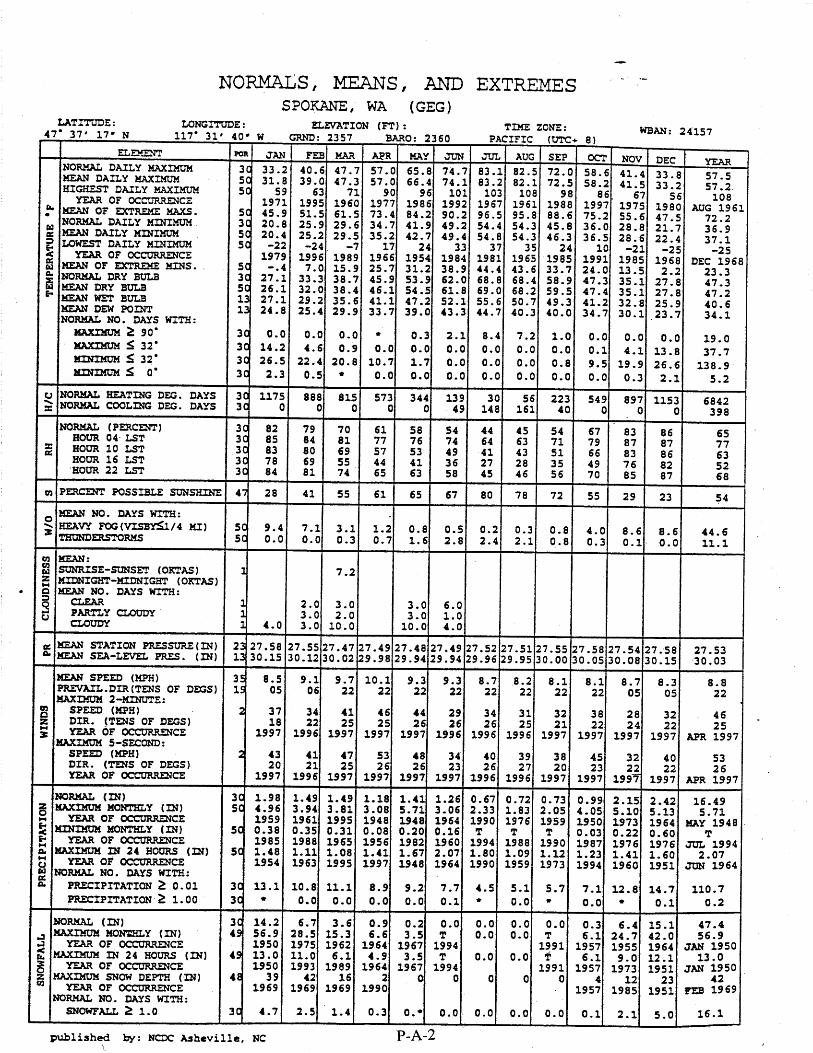
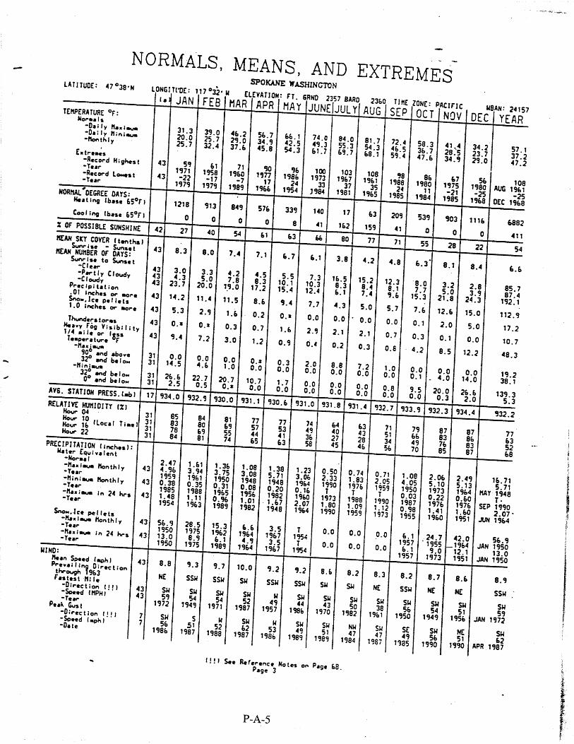
ANNEX B

HIGHWAY WHEAT AND BARLEY FLOWS WITH AND WITHOUT THE SNAKE RIVER WATERWAY

The four figures presented in this Annex show highways used to transport wheat and barley to railroad- or river-port-based grain elevators. Maps of wheat and barley flows are presented for the Existing Condition Pathway (Base Scenario) and the Natural River Drawdown Pathway (No-Barge Scenario). The highways are color coded to indicate the number of bushels transported over eastern Washington roads. Grain volumes can be translated to the number of trucks by assuming that each bushel weighs 60 pounds, and the truck capacity is 26 tons. The maps were originally presented in the publicly funded EWITS Report Number 23 (Jessup, Ellis, and Casavant, 1997), which may be obtained at the website for Washington State Unversity (http://ewits.wsu.edu/frames5.htm).

brownj

brownj

Figure 8. Optimized Wheat Flows on Eastern Washington Highway (Base Scenario)

brownj

1 - 2,000,000 2,000,0001 - 5,000,000 5,000,001 - 15,000,000 15,000,001 - 40,737,357

brownj

Wheat Flows (bu.)

brownj

brownj

brownj

brownj

brownj

brownj

Figure 9. Optimized Wheat Flows on Eastern Washington Highway (NoBarge Scenario)

brownj

brownj

1 - 2,000,000 2,000,0001 - 5,000,000 5,000,001 - 15,000,000 15,000,001 - 46,851,370

brownj

Wheat Flows (bu.)

brownj

brownj

Figure 10. Optimized Barley Flows on Eastern Washington Highway (Base Scenario)

brownj

1 - 1,000,000 1,000,0001 - 2,000,000 2,000,001 - 4,000,000 4,000,001 - 6,225,308 Feedlots

brownj

Barley Flows (bu.)

brownj

brownj

Figure 11. Optimized Barley Flows on Eastern Washington Highway (No-Barge Scenario)

brownj

1 - 1,000,000 1,000,0001 - 2,000,000 2,000,001 - 4,000,000 4,000,001 - 17,154,211 Feedlots

brownj

Barley Flows (bu.)

brownj

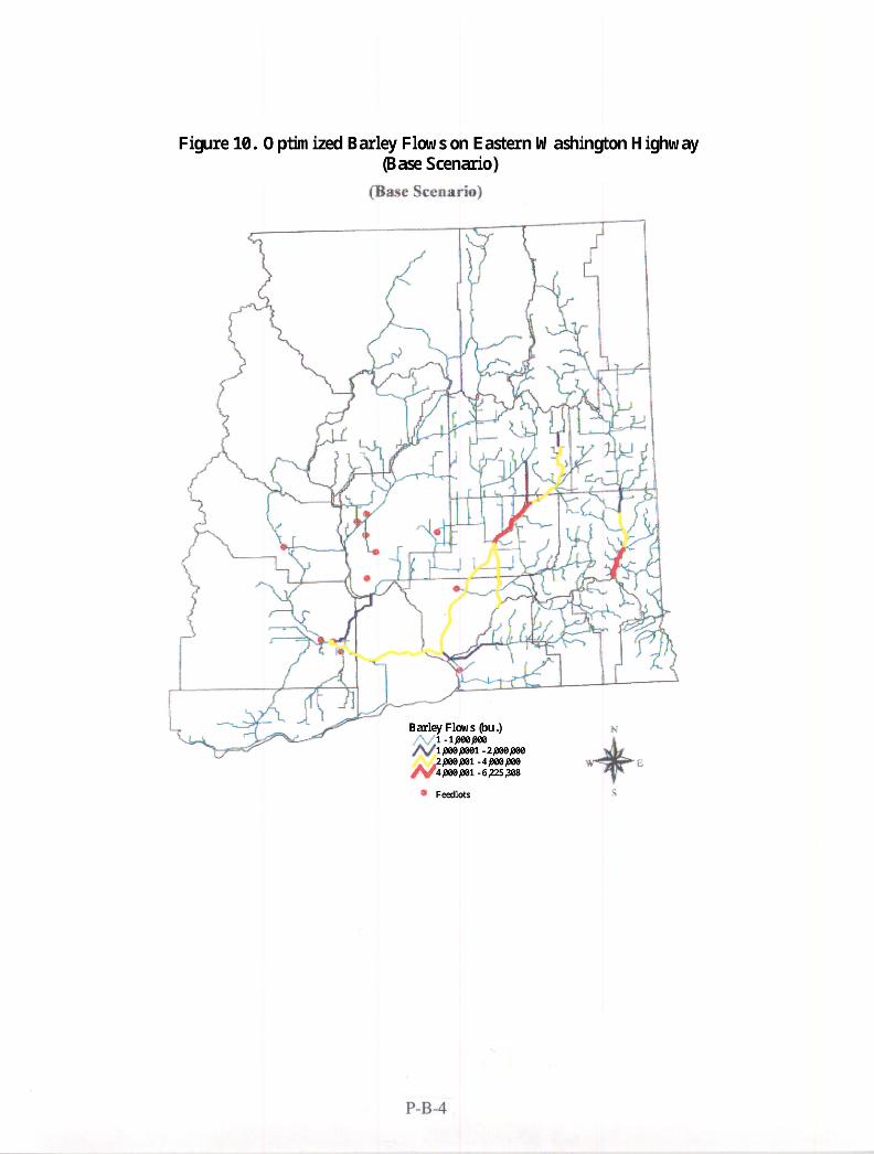
ANNEX C

PREDICTED PM10 CONCENTRATIONS FOR STORM EVENTS

P-C-1

The figures in this Annex show the distribution of predicted 24-hour PM10 concentrations for eastern Washington storms. The predictions were developed from CP3 modeling and were presented in Claiborn et al., 1998. Data used to develop the plots were provided by Brian Lamb, Laboratory for Atmospheric Research, Washington State University, Pullman, Washington. Additional information on the CP3 program may be obtained at http://coopext.cahe.wsu.edu/ncp3/.

P-C-3

24-Hour Predicted PM 10 Concentrations for September 11, 1993

µg/m3

Spokane

KennewickIceHarbor

LowerMonumentalLittleGooseLowerGranite

0 km 50 km 100 km 150 km

50

100

150

200

400

800

1600

3200

brownj

brownj

P-C-2

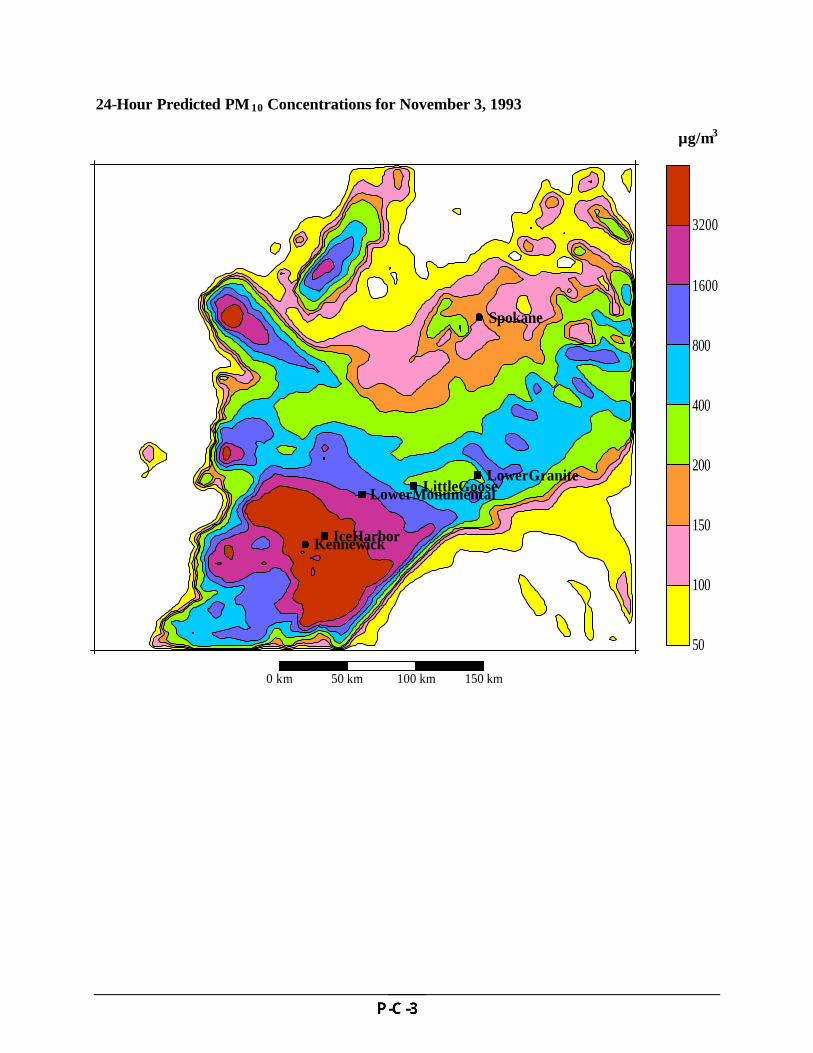
P-C-4

24-Hour Predicted PM 10 Concentrations for November 3, 1993

µg/m3

Spokane

KennewickIceHarbor


0 km 50 km 100 km 150 km

50

100

150

200

400

800

1600

3200

brownj

brownj

P-C-3

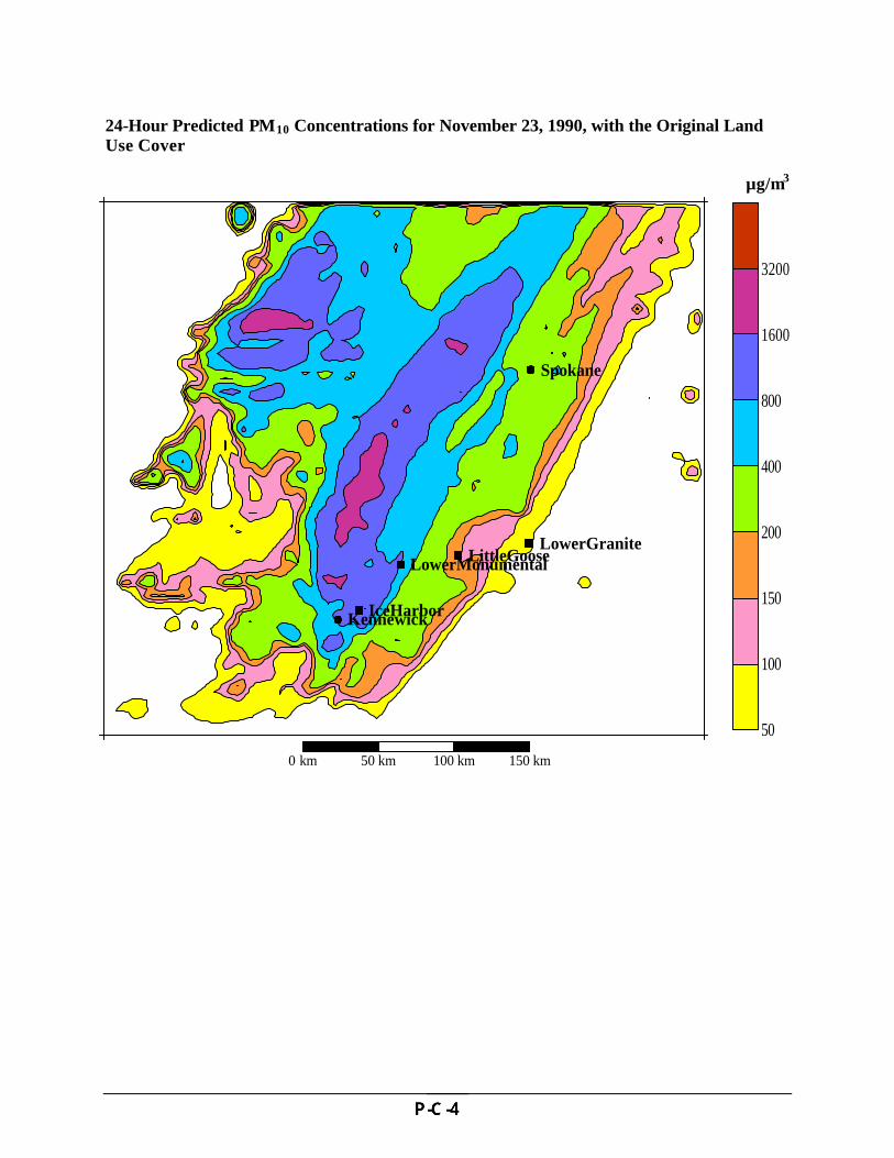
P-C-5

24-Hour Predicted PM10 Concentrations for November 23, 1990, with the Original Land Use Cover

µg/m3

Spokane

KennewickIceHarbor


50

100

150

200

400

800

1600

3200

0 km 50 km 100 km 150 km

brownj

brownj

P-C-4

P-C-6

24-Hour Predicted PM 10 Concentrations for November 23, 1990, for Snake River Reservoir Sediment Emissions

µg/m3

*Not to scale.

Spokane

Kennewick

Lower Monumental

Lower Granite

1

2

3

4

0 km 50 100 150

brownj

brownj

P-C-5

P-C-7

24-Hour Predicted PM 10 Concentrations for November 23, 1990, with the Modified Land Use Cover

µg/m3

Spokane

KennewickIceHarbor


50

100

150

200

400

800

1600

3200

0 km 50 km 100 km 150 km

brownj

brownj

P-C-6

ANNEX D

POPULATION DISTRIBUTION MAP

walla walla district - united states army feasibility study is to evaluate and screen structural...

Documents