wages, experience and seniority - ucl - london's global …uctpb21/cpapers/wagesexpsen.pdf ·...

Review of Economic Studies (2005)72, 77–108 0034-6527/05/000500077$02.00c© 2005 The Review of Economic Studies Limited

Wages, Experience and SeniorityCHRISTIAN DUSTMANN and COSTAS MEGHIRUniversity College London, Institute for Fiscal Studies and CEPR

First version received January2001; final version accepted November2003(Eds.)

In this paper we study the sources of wage growth. We identify the contribution to such growth ofgeneral, sector specific and firm specific human capital. Our results are interpretable within the context ofa model where the returns to human capital may be heterogeneous and where firms may offer differentcombinations of entry level wages and firm specific human capital development. We allow for thepossibility that wages are match specific and that workers move jobs as a result of identifying a bettermatch. To estimate the average returns to experience, sector tenure and firm specific tenure within thiscontext, we develop an identification strategy which relies on the use of firm closures. Our data source isa new and unique administrative data-set for Germany that includes complete work histories as well asindividual characteristics. We find positive returns to experience and firm tenure for skilled workers. Thereturns to experience for unskilled workers are small and insignificant after 2 years of experience. Theirreturns to sector tenure are also zero. However, their returns to firm tenure are substantial.

1. INTRODUCTION

In this paper we study the growth of wages of young workers in Germany. Knowing the extentand reasons for individual wage growth over the life cycle is important for a number of areasin Economics. Just to mention two examples: first, it is a key element to understanding anddesigning active labour market programmes. Many such programmes offer temporary (andoften subsidized) work opportunities. Examples are the New Deal in the U.K. and the Swedishprogrammes as well as a number of programmes in Germany. These programmes are based onthe assumption that general skills are sufficiently enhanced while working, so as to render theworkers employable without a wage subsidy. Thus the success of these programmes dependson how skills improve on the job for the target population, and whether this skill enhancementis transferable across jobs. Second, it is a key to understanding the benefits and costs of jobmobility. This in turn matters for a number of policy issues, including the design of pensionpolicies, relating for example to final salary schemes.

As a result of this widespread interest, a large body of empirical research has focused onobtaining estimates for the returns of experience and seniority.1 Our study uses a new and uniqueadministrative data-set with a number of features that are important for our analysis and allow usto avoid many problems encountered in earlier work in this field. In our model wages grow due tolearning by doing, which may be heterogeneous across individuals. Moreover, since firms offerdifferent career profiles and because we allow for match specific effects on wages, investmentstake the form of searching for the firm with the most desirable learning by doing characteristics(career structure).2

1. SeeAltonji and Shakotko(1987), Topel(1991), Topel and Ward(1992), Neal(1995), Parent(1995) andAltonjiand Williams(1996, 1997) among others.

2. In general the acquisition of human capital on the job may be a result of decisions to invest as well as purelylearning by doing. Examples of models with explicit investment in Human Capital areBen-Porath(1967), Blinder andWeiss(1976), Rosen(1976) andJovanovic(1979), amongst others. Examples of models where learning is a by-productof work are given inRosen(1972). Killingsworth (1982) presents a model unifying the features of the earlier literature.

77

78 REVIEW OF ECONOMIC STUDIES

Thus the framework we present leads to a wage equation, which depends on the number ofperiods the individual has worked (experience), the time spent in the sector (sector tenure) andthe time spent in the firm (tenure). The impact of these factors is allowed to be heterogeneousacross individuals, which leads to a correlated random coefficients model for wages. Randomcoefficient models are not new of course. TheWillis and Rosen(1979) model on the returns toeducation and theHeckman and Sedlacek(1985) model of self-selection to the labour market(based on Roy), are early empirical examples.Heckman and Robb(1985) discuss the estimationof such models in the context of evaluation of treatment effects andBjorklund and Moffitt(1987)apply these ideas to the estimation of the returns to training in Sweden. More recentlyImbensand Angrist(1994) andHeckman(1995) consider the interpretability of instrumental variableestimation in the context of random coefficient models.

We discuss how the population average returns to experience and tenure can be identifiedgiven individual and firm behaviour. Our approach is partly based on using displaced workersdue to firm closure, thus allowing us to distinguish wage growth due to learning by doing fromwage growth due to endogenous job mobility, which leads to improved job matches.3 However,we recognize that even for displaced workers both the fact that they accepted a new job as well asexperience itself are endogenous at job entry. We use age as an excluded instrument to allow forsuch endogeneity by developing an estimator based on the control function approach ofHeckmanand Robb(1985), and allowing for heterogeneous returns to experience, sector tenure and firmtenure.4

Our data allows us to observe all transitions that take place between jobs and betweenwork and unemployment from the start of the worker’s labour market career. All wageobservations relate to a particular job and are not averaged across jobs; thus when an individualchanges employment we observe the new wage at which he is appointed. Because the data isadministrative, there is practically no attrition and most probably much less measurement errorthan that in questionnaire based survey data. In addition, for any firm that closed down andemployed any of our workers within our observation window, we know the year of closure.

From the overall database, we extract a sample of workers entering the labour marketbetween 1975 and 1995. The oldest worker in our sample is 35. The use of such a young samplehas the advantage that we can focus on the age group where most of the job mobility and life-cycle wage growth takes place. Since this database came into existence in 1975, our sampleselection ensures that we choose those cohorts for which the complete labour market history ofall individuals is observed.

Our analysis is carried out separately for skilled individuals who have received formalvocational training (apprenticeship) and for those who have not—the unskilled. This revealsimportant differences between the groups, which is key to the design of policy such as activelabour market programmes.

We find that the returns to experience for the skilled workers can be substantial. In the first2 years of work, following formal training, wages grow at 7% and then at 6% a year. The returnsdecline thereafter, but even in the longer run experience leads to a wage growth of 1·2% a year.For the unskilled workers there are substantial returns in the first 2 years (10% and 8%) but theybecome effectively zero beyond 3 years of work. In addition to this growth due to experience,the wages of unskilled workers also grow early on via improved job matches achieved by jobmobility; this, however, is not an important source of growth for the skilled workers. The returns

3. Displaced workers have been used before to control for selection due to unobserved heterogeneity. ExamplesincludeKletzer(1989) andGibbons and Katz(1992). Kletzer also includes among the exogenously displaced individualsthose fired from firms that continue as a going concern.

4. The approach we follow is parametric and is similar toHeckman and Vytlacil(1998). General non-parametricidentification issues in these models are discussed inFlorens, Heckman, Meghir and Vytlacil(2002).

DUSTMANN & MEGHIR WAGES, EXPERIENCE AND SENIORITY 79

to remaining in the same sector (sector or industry tenure) are 1% a year for skilled workersand basically zero for the unskilled. On the other hand the returns to remaining with the sameemployer (tenure) for the unskilled workers are quite high for the first 5 years (4% a year) but zerothereafter, despite the fact that we control for sector tenure. Skilled workers have lower returnsto tenure(2·4%). Thus in Germany unskilled workers benefit most by finding a good match andremaining with it. An implication is that if a labour market programme is to be effective for theunskilled it will have to make sure placements are long lasting. For skilled workers human capitalis transferable and tenure is not as important. This may be due to the nature of the apprenticeshipsystem. A series of sensitivity tests demonstrate the robustness of these results to alternativedefinitions of displacement.

This paper proceeds as follows: in the next section we present a theoretical framework,where we describe the model and discuss identification of the parameters of interest underdifferent theoretical assumptions. This is followed by a section where we describe the data andthe sample we use, and provide descriptive features of job mobility and wage growth for youngworkers in Germany. We then present our empirical results. Finally, we summarize our findingsand their implications in the concluding section.

2. THEORETICAL FRAMEWORK

Human capital is composed of transferable skills, sector specific skills and firm specific skills.Workers are assumed to obtain the returns to the first two and to share the returns to the latter,based on the proportion invested for its acquisition by the worker relative to the firm.5 Thusdefine byHa

i f t that part of human capital for which workeri with education typeai , workingin firm f during periodt gets paid for. This is related to the number of periods the worker hasworked in firm f (T F

i f t ), in sectors (T Sit ) and overall(TG

it ) by the function

ln Hai f t = g(TG

it | ai ) + ηi t TGit + s(T S

it | ai ) + εi t TS

it + f (T Fi f t | ai ) + νi f t T

Fi f t + mi f t ,

whereg(TGit | ai )+ηi t TG

it is the log of general transferable human capital,s(T Sit | ai )+ εi t T S

it isthe log of human capital specific to the sector, andf (T F

i f t | ai )+νi f t T Fi f t is the log of firm specific

human capital whose return is enjoyed by the worker. The termηi t reflects individual specificreturns to general experience. The termsmi f t andνi f t reflect the match specific productivity andcareer structure. Thus the value of a match (given experience and tenure) is characterized by afirm/worker specific component of the wage levelmi f t and growthνi f t . We expect these to benegatively correlated in equilibrium.6 Finally, ai is the educational category of individuali . Notethat the random returns may be persistent over time or even fixed for each individual.

We assume learning by doing is passive and takes place within a job. The individual canchoose the firm with the desired career profile, the sector in which he works and whether to workor not in a particular period.

In our empirical analysis we distinguish between two skill categories: those withapprenticeship education(ai = 1) and those without(ai = 0). The market price for humancapital of typea is r a

t . The observed wage of individuali , working in firm f , in time periodt

5. SeeBecker(1993). Equilibrium models that explain why workers get rewarded for specific training and theway the costs and the returns are shared have been developed under many different assumptions. Some examples includeHashimoto(1981), Datta(1995), Harris and Felli(1996) andScoones and Bernhardt(1996).

6. No restrictions are imposed on the way that the unobservablesηi t , εi t , mi f t andνi f t are correlated. Also notethat the firm’s willingness to hire the worker or otherwise is reflected in the overall value of the match. Given the paythat this implies it is then up to the worker to take the job or not. SeeFarber(1983) for an alternative where there may beexcess supply of workers, in his case to union jobs.


and of skill levela is wi f t = r at Ha

i f t eei t whereei t represents either measurement error and/or

transitory shocks to human capital. The log wage for an individuali in periodt can be written as

ln wi f t = ln r at +g(TG

it | ai )+s(T Sit | ai )+ f (T F

i f t | ai )+ηi t TGit +εi t T

Sit +νi f t T

Fi f t +mi f t +ei t .

(1)Draws of the match specific effects(ui f t = {mi f t , νi f t }) will in general be correlated acrossfirms, due to individual unobserved characteristics. Preferred draws ofui f t will drive mobility.7

2.1. Identifying the return to experience

Comparing the wages of workers with different levels of experience is known to provide biasedresults for the returns to experience (see, for example,Altonji and Shakotko(1987), Topel(1991),Altonji and Williams(1996)) for at least two reasons. First, because some of the differences maybe attributed to better matches achieved by workers who have been in the labour market longer.Second, because high-ability workers are likely to have a stronger labour market attachment andhence end up with more experience. In our model, there is a further source of a potential biasin the estimation of theaveragereturns to experience: workers with higher returns to experienceare likely to spend less time out of the labour market, because for them the opportunity cost ofnot working is higher. This will lead to a positive correlation of the returns to experienceηi t withexperienceTG

it .The dynamic selection induced by this process will generally distort the returns to

experience, and it is difficult to model (seeEckstein and Wolpin, 1989). Topel (1991) suggestsestimating the returns to experience by using the wages of those starting a new job and whotherefore have zero tenure. However, workers who start a new job are a mixture of workers whoare improving on their previous wage, workers who have been fired from an ongoing firm, andworkers who have been displaced because the firm actually closed down, all of whom find thecurrent offer more attractive than unemployment.

We resolve this problem by using only those workers who start a new job following adisplacement caused by the closure of a firm.8 We will term these displaced workers. InAppendixA we show why exogenous displacement can simplify the problem. The basic intuition is simple:if, as we assume, firm closure is exogenous conditional on our observables, then workers whohave thus been displaced are a random sample of the workforce and are not selected into new jobson the basis of their past choices, but just on whether this job offer is preferable to unemployment.Thus our approach identifies the returns to experience by comparing the wages of workers withdifferent levels of experience, who start a new job following displacement.

Of course even for this sample there is still the well-known ability bias problem (experienceis correlated with the permanent part of the unobservables), and the problem that only thosedisplaced workers receiving good enough offers will take up employment.9 We solve theseendogeneity/selection problems by using age effects as exclusion restrictions, combined witha control function estimator on the displaced sample, where we use residuals from an experienceand participation reduced form to allow for the endogenous job acceptance and experience.10

In what follows, we state a set of assumptions that justify our approach and present theestimation procedure we use.

7. Farber(1994) among others provides interesting evidence on the importance of matching for mobility.8. This strategy is based on a number of assumptions, which we list below.Gibbons and Katz(1992) also argue

that displaced workers can be used to control for selection in a matching context. They apply their strategy in a bid toexplain inter-industry wage differentials.

9. By ability bias we refer to the bias generated by the tendency of individuals who are more productive, or havea higher return to experience, to spend more time in employment and hence be more experienced for any given level ofpotential experience.

10. SeeHeckman and Robb(1985).


2.2. Assumptions

Our approach for estimating the average returns to experience for the workforce population isbased on the following assumptions:

A.1 Workers cannot predict a closure before joining the firm. Moreover, they cannot predicta closure when working in the firm if the closure is more than a year away.

AssumptionA.1 ensures that there is no self-selection of a particular type of worker (interms of unobserved characteristics) into firms that are subsequently observed to close down.Since we can predict firm closure in terms of certain observables, we can carry out a sensitivityanalysis. In particular, we compare the results we obtain using all closures, to those obtainedusing closures of older firms only, which have much lower exit rates. We develop this idea at theend of the empirical section.

There may also be selection of workers leaving the firm before closure. In our data weknow whether a firm closed down, independently of whether the worker remained employed byit. Hence, we can define a displaced worker as someone who left a firm which closed down inx amount of time following his departure, wherex is chosen by us.A.1 assumes there are noselective departures related to the closure earlier than a year before the event. In the empiricalsection we develop a sensitivity test, based on alternative definitions of this time window. Inparticular, we consider a worker as displaced if the firm closes down within different periods ofhis departure, and we compare the results.

A.2 Workers and firms have full information on the quality of the match.AssumptionA.2 excludes learning about the quality of the match so as to simplify the

interpretation of the results.11

A.3 Exclusion restriction: For the population of young displaced workers(Di t = 1) theunobservables in the wage equation are mean independent of age, conditional on exogenousobservable characteristicsXi t (including school education, apprenticeship status, and time).Thus,

E(ηi t | agei t , Xi t , Di t = 1) = E(εi t | agei t , Xi t , Di t = 1) = 0

E(νi f t | agei t , Xi t , Di t = 1) = E(mi f t + ei t | agei t , Xi t , Di t = 1) = 0.

This assumption ensures that age does not affect wage offers facing exogenously displacedindividuals with the same observables.12 This assumption may not be true in the overallsample since the quality of matches may improve with age because older workers will havebeen sampling jobs for longer. The key point of this assumption is that post-displacement,workers have lost all earlier match advantages that would have been achieved through search(search capital) and that workers have to start afresh. As a result, being an older or youngerworker (within the relatively narrow age range we consider—remember that workers are lessthan 35 years old) does not in itself confer any advantage in obtaining a better match post-displacement. Implicit also in this assumption is the exclusion of cohort effects from wages.13

We also require a condition that ensures that the instruments we use can explain participationand experience and also induce independent variation in the two predictions. Our requirement isthat age has an impact on participation in the labour market. We expect this to be the case since

11. In the presence of learning about the quality of the match it may not be possible to disentangle the growthof wages due to an increase in productivity from growth due to increased remuneration as the quality of the match isrevealed. SeeNagypal(2002) for a recent attempt to distinguish learning by doing from learning about match quality.

12. Since the conditional mean of the unobservables is assumed to be equal to zero, which is their unconditionalpopulation mean, these orthogonality conditions identify the population mean of the returns to experience.

13. Note that age+ cohort= year. Since the model also includes time effects, including cohort and time would bethe same as including age, at least linearly.


labour market attachment changes with age for a variety of reasons, including family formation,housing, better job matches, etc.

The instruments will also have explanatory power for experience since actual experienceis the sum of past employment outcomes. If age effects on participation are sufficientlynon-linear this exclusion restriction provides all the necessary identifying information. Inpractice this is the case. In addition, we can also exploit the fact that the impact of agechanges with potential experience by using age/potential experience interactions as instruments.Since potential experience is age minus years of education in practice this amounts to usingage/education interactions as additional instruments. This leads us to the rank condition, whichcan be stated as:14

A.4 Rank condition: Define byϑG the vector of coefficients on all excluded instruments inthe experience reduced form and byϑ P the vector of coefficients of these same variables in theparticipation reduced form. The rank condition of identification requires that the matrix[ϑGϑ P

]

has rank 2.We present a formal test of the rank condition, which is easily satisfied in our data.The exclusion restriction and the rank condition are not sufficient for identifying average

returns in models with heterogeneous returns which may be correlated with the endogenousvariables.15 In addition we require the followingcontrol functionassumptions that define howthe mean of the unobservables relate to experience(TG), sector tenure(T S) and job acceptancefollowing a closure(P).

A.5 For the sample of displaced workers(Di t = 1) starting a new job16 following a firmclosure, we assume that

E(mi f t + ei t | agei t , Xi t , Di t = 1, Pi t = 1, TGit , T S

it , T Fi f t = 0)

= δG(ci t )υGit + δP(ci t )υ

Pit , (2)

E(ηi t | agei t , Xi t , Di t = 1, Pi t = 1, TGit , T S

it , T Fi f t = 0) = γ G(ci t )υ

Git + γ P(ci t )υ

Pit , (3)

E(εi t | agei t , Xi t , Di t = 1, Pi t = 1, TGit , T S

it , T Fi f t = 0) = κG(ci t )υ

Git + κ P(ci t )υ

Pit , (4)

where Pi t = 1 represents those accepting a new job following displacement,ci t is potentialexperience,17 andυG

it = TGit − E(TG

it | agei t , Xi t ) andυPit = Pi t − E(Pi t | agei t , Xi t ) are

residuals from an experience and participation reduced form. The control function assumption isfamiliar from standard selection models (e.g.Heckman, 1979). A sufficient (but not necessary)condition for this assumption to hold is that the instrument is independent of the errors. Subject tothe exclusion restrictionsA.3 and the rank conditionA.4, thiscontrol functionassumption allowsus to identify the average return to experience and sector tenure based on the wage obtainedfollowing displacement. We allow the coefficients (theδ’s, γ ’s andκ ’s) to depend on potentialexperienceci t because the distribution of experience will vary with the number of years thatthe individual has been in the labour market. For example, a person with 5 years of potentialexperience can have no more than 5 years of actual experience. Moreover, as implied by (3) and(4), the above formulation recognizes that past and present employment outcomes may dependon the returns to experience(ηi t ), and sector tenure(εi t ).

14. For a recent application of a similar idea see Blundell, Duncan and Meghir (1998) and for the theory of ranktests seeRobin and Smith(2000).

15. SeeGaren(1984), Heckman and Robb(1985), Heckman and Vytlacil(1998), Card(2001) andFlorenset al.(2002).

16. All these workers have zero tenure at that point.17. Potential experience is the number of years that the person could have worked for pay since the end of full time

education. SinceX includes education and we also condition on age,ci t is implicitly included in the set of conditioningvariables.


Assumption A.5 implies that conditional on experience, job acceptance followingdisplacement and the other observable characteristics, a sector tenure residual is not required.We provide a test of this exogeneity assumption, which turns out to be easily acceptable in ourdata. This is not surprising, since we allow for the returns to sector tenure to affect the mobilityand work decisions (see equation (4)). We discuss the test in the empirical section.

Finally, note that identification does not rely on linearity of the control function. There aretwo key elements in the identification of the average treatment effect using the control functionestimator.18 First an instrument which is continuous or takes on many discrete values. In a non-parametric setting this instrument must satisfy a generalized rank condition which implies thatit can explain any function of the endogenous variable. Second, that the dependence of theconditional mean of the unobservables given the endogenous variables and the instrument isonly a function of the residualsυP andυG and not of the endogenous variable and the instrumentseparately.Florenset al. (2002) develop arguments relating to the non-parametric identifiabilityof models with heterogeneous impacts of continuous variables such as experience or tenure.

We do not impose any arbitrary functional form assumptions on the residuals that wouldforce them to have independent variation. The residuals originate from simple linear regressions.We just require the testable rank conditionA.4 to be satisfied. Finally note that there are furtherstructural restrictions linking participation and experience but we do not exploit these here.

2.3. Implementation of the estimation method

To implement this estimation approach, we start by estimating reduced forms for participation,and for experience at the beginning of the current period. These are estimated on all individuals(independently of their current or past work status) using ordinary least squares (OLS). Aseparate reduced form is estimated for each skill group. The experience reduced form for eachskill groupa (apprentices and non-apprentices) is

TGit = αaG

0 +αaG1 agei t +αaG

2 ci t +αaG3 agei t ×ci t +ad′

i t αaG4 +(adi t ×ci t )

′αaG5 +x′

i t ξaG

+υGit . (5)

The variablesad are age indicators.19 The x variables are the year indicators and the level ofschool education. The variableci t is potential experience of individuali in calendar periodt . Wealso estimate a reduced form participation equation (job acceptance), which has the same form.Having estimated the reduced forms, we compute the respective residualsυG

it andυPit .

The next step involves writing wages as lnwi t = E(ln wi f t | agei t , Xi t , Di t = 1, Pi t = 1,TG

it , T Sit , T F

i f t = 0)+e∗

i t , by applying the assumptions (2), (3) and (4) when taking the conditionalexpectation of wages in (1). We assume that the parameters on the residual terms in (2) and (3)(δG(ci t ), δ

P(ci t ), γG(ci t ), γ

P(ci t ), κG(ci t ), κ

P(ci t )) are linear in potential experience.20 Thuswe obtain the following regression that can be estimated using ordinary least squares on thesubsample of those starting a new job following displacement:

ln wi f t = ln r at + g(TG

it | ai ) + s(T Sit | ai ) + x′

i t γa

+ δG1 υG

it + δG2 ci t υ

Git + δP

1 υPit

+ δP2 ci t υ

Pit + γ G

1 TGit υG

it + γ G2 ci t T

Git υG

it + γ P1 TG

it υPit + γ P

2 ci t TGit υP

it

+ κG1 T S

it υGit + κG

2 ci t TS

it υGit + κ P

1 T Sit υ

Pit + κ P

2 ci t TS

it υPit + e∗

i t . (6)

Any estimator that includes the control functions (residual terms) will be referred to as acontrol function estimator.

18. See alsoNewey, Powell and Vella(1999).19. To test for non-linearities, we test for the exclusion of the age dummies, given the inclusion of the linear age

term.20. For example,δG(ci t ) = δG

1 + δG2 ci t .


The specification ofg(TGit | ai ) and s(T S

it | ai ) is stated in the empirical section. Theinteractions of these residuals with experienceTG

it and sector tenureT Sit control for self-selection

due to heterogeneous returns to experience and sector tenure. Finally, as explained above, therelationship of these residuals to the unobservables in wages are likely to be changing withpotential experienceci t .21 We allow for this by interacting all terms withci t .

2.4. Estimating the return to tenure

In estimating the returns to tenure, we use wages in jobs that follow firm closures. This isnecessary because the existence of match specific returns to tenure may imply the accumulationof search capital which may be confused with returns to tenure. Consider wages adjusted foraverage growth due to experience and sector tenure. These are

˜ln wi f t = ln wi t − ln r at −

g(TGit | ai ) −

s(T Sit | ai ), (7)

where ln r at , g(TG

it | ai ) and s(T Sit | ai ) are the pre-estimated aggregate growth of wages and the

experience and sector tenure components, respectively.The adjusted wage is then given by

˜ln wi f t = f (T Fit | ai ) +

[ηi t T

Git + εi t T

Sit + νi f t T

Fi f t + mi f t + ei t

](8)

whereei t reflects estimation error from the first stage as well as the original errorei t .With heterogeneous returns and/or heterogeneity that varies over time first differencing does

not help. Thus, to estimate the returns to tenure similar to the case of experience, we need tomodelE

[ηi t TG

it + εi t T Sit + νi f t T F

i f t + mi f t + ei t | age, TGit , T S

it , T Fi f t , ci t

]. Relative to the case

where tenure is zero, this expression includes an extra term(νi f t T Fi f t ). Moreover, we need to

model the relationship between tenure and all the residual terms. Thus the assumptions we madeearlier are updated to22

E(mi f t + ei t | agei t , Xi t , Di t = 1, Pi t = 1, TGit , T S

it , T Fi f t ) = λG(ci t )υ

Git + λP(ci t )υ

Pit + λT (ci t )υ

Tit , (9)

E(TGit ηi t | agei t , Xi t , Di t = 1, Pi t = 1, TG

it , T Sit , T F

i f t ) =

[ρG(ci t )υ

Git + ρP(ci t )υ

Pit + ρT (ci t )υ

Tit

]TG

it , (10)

E(T Sit εi t | agei t , Xi t , Di t = 1, Pi t = 1, TG

it , T Sit , T F

i f t ) =

[θG(ci t )υ

Git + θ P(ci t )υ

Pit + θT (ci t )υ

Tit

]T S

it , (11)

E(T Fi f t νi f t | agei t , Xi t , Di t = 1, Pi t = 1, TG

it , T Sit , T F

i f t ) =

[ξG(ci t )υ

Git + ξ P(ci t )υ

Pit + ξT (ci t )υ

Tit

]T F

i f t (12)

whereυTit is the residual from the tenure reduced form and where as before the coefficients of

each of the residuals are linear functions of potential experience (ci t ).The tenure reduced form will be of the same form as (5). We expect age to affect mobility

between jobs and hence tenure because mobility costs will be higher for older individuals dueto family and housing among other things. Thus age effects and age interacted with potentialexperience should matter for tenure. More generally, identification relies on the matrix ofcoefficients on the age effects and age effects interacted with potential experience from thethreereduced forms (participation, experience and tenure) having rank three. The rank condition ismore demanding than for estimating the effects of experience alone. Thus overall the conditionsfor identifying the returns to tenure are more stringent than the conditions required for identifyingthe returns to experience. The rank condition is amply satisfied in the data even with the threereduced forms, as shown in what follows. Identification is further aided by the fact that the

21. If nothing else, the maximum number of years of experience increases with potential experience.22. Note thatDi t = 1 means that the worker had been displaced in the job immediately preceding the current one.


returns to experience and sector tenure can be estimated at a first step, under weaker conditionsby relying on the first job record, where tenure is zero (as discussed above).

Implementation of the estimator involves regressing the adjusted wage( ˜ln wi f t ) on thefunction of tenure( f (T F

i f t | ai )) and on all pre-estimated residual terms shown in the equationsabove. The residuals are estimated based on linear reduced forms for experience, participationand tenure with the same specification as in equation (5).

Standard errors and inference

Our approach requires that the standard errors are corrected for generated regressor bias. Wealso need to account for serial correlation and heteroscedasticity, both of unknown form. Sincecomputing the standard errors analytically can be very cumbersome in these circumstances wehave used the block bootstrap where we treat each individual as a sampling unit, thus allowing forarbitrary serial correlation and heteroscedasticity. We bootstrap the entire estimation procedurethus allowing for the stage-by-stage nature of our estimator. This also allows us to evaluatewhether there is any important small sample bias in our approach (seeHall and Horowitz(1996),Horowitz(2001)).23 Moreover, many of the test statistics we present use bootstrap critical values.To the extent that the tests are pivotal (i.e. their asymptotic distribution does not depend onunknown parameters), this will provide small sample refinements. Otherwise this procedure isequivalent to using the asymptotic distribution.

3. THE DATA

The data we use is a 1% sample from the German Social Security records (IAB data), which hasbeen supplemented by information from the official unemployment records. We only considermale workers in West Germany. This data is available for the years 1975–1995 (seeBender,Hilzendegen, Rohwer and Rudolph, 1996, for details). Over this period, it records for eachworker the exact date of any change to a new job or to (and from) unemployment. Furthermore, itcontains an obligatory yearly entry for each worker. Thus an accurate calendar of labour marketstatus is provided with minimal, if any, measurement error for each worker. It further providesinformation about whether a worker is on an apprenticeship training scheme.

Wages are recorded in the following fashion. If the worker does not change firm over thecalendar year, the average daily wage is recorded over this period. If the worker changes jobs, therecord includes the average daily wage for the period from the start of the calendar year (or thestart of the spell, whichever is more recent) to the date of termination of employment at the firm.Then we obtain an average daily wage from the beginning of the new employment spell to theend of the calendar year (or to the end of the employment spell, whichever comes sooner). Hencethe wage informationalwaysrelates to a single firm, and never covers more than one calendaryear. We deflate wages by the German consumer price index. In addition, we use data on age,educational qualifications and industry. Thus the data allows us to construct very accurate workandearnings histories. The accuracy of our work history information contrasts with informationbased on recall and individual based responses (such as the U.S. NLSY and PSID or the U.K.BHPS).

The data does not cover the entire German labour force, as the self-employed and civilservants do not pay social security contributions, and are therefore excluded. Moreover, as withmany administrative data-sets, the data is top coded. In our analysis, we consider only young

23. Fitzenberger and Kurz(2003) provide a recent application in the use of the block bootstrap in the context ofestimating wage equations.


individuals who went through apprenticeship training, and individuals who did not receiveany further training after school. Top coding hardly affects the wages of workers in thesegroups.24

The database contains also information on the firm in which each worker is employed. Usingseparate information on the firm we can link in the year that the firm started and closed down.When the firm has many establishments the data refers to one establishment and not to a wholefirm. However, for simplicity we just use the term firm throughout.

The sample

From this database, we construct a sample of young male workers whom we observe from theentry to the labour force onwards. To ensure that we do not miss out early employment spells,we restrict our sample to workers who were not older than 15 in 1975 (which is the minimumcompulsory full time schooling age).

We distinguish between two levels of qualification: workers who go through anapprenticeship training scheme early on in their careers, and workers who do not acquire anyfurther formal training after school (which could be a high school degree with 13 years ofschooling, or a lower secondary degree with 9–10 years of schooling), or who drop out of thetraining scheme. We refer to these two samples as theskilled and theunskilledsample. Thelongest labour market history in our data-set is 19 years, and the shortest 2 years. Our finalsample consists of 25,649 skilled workers, with 204,458 employment records, and 7264 unskilledworkers, with 55,924 employment records.25

3.1. A descriptive analysis of wage growth and job mobility

We provide some information on the institutional background, the education system and wagesetting in Germany inAppendix B.26 In this section, we describe the basic features of jobmobility and wage growth in our sample.

Mobility

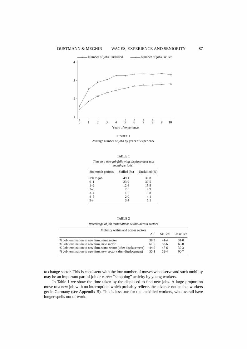
In Figure1, we illustrate job mobility for the first 10 years of labour market experience, wherewe break down our sample into the two different educational categories. The figure shows thatmobility is lower for better educated workers throughout. After 10 years, an unskilled worker hasheld 3·4 jobs on average, while a skilled worker has held 2·8 jobs. The figure also shows that theaverage number of jobs held in Germany increases only during the first 4–5 years, and flattensout afterwards. These numbers confirm that mobility in Germany is relatively low; this contraststo the U.S. for example where, on average, workers hold their 7-th job after 10 years of labourmarket experience (seeTopel and Ward, 1992).

In Table2 we show the percentage of job moves that result in a job within the same sectorand in a different sector.TableB1 in AppendixB provides the list of the 15 sectors we considerand the proportion of workers in our sample employed in each over the entire time period weconsider. Here it emerges that the majority of moves between firms involves a change in sector.However, when it comes to the moves caused by closure the proportion staying in the same sectorrises. Thus among those making a decision to move between firms a large proportion also decides

24. Less than 1% of our sample population experience a right censoring later in their career.25. We delete the few individuals who have one or more part time spells.26. Burda and Mertens(2001), Bender, Dustmann, Margolis and Meghir(2002) andFitzenberger and Kurz(2003)

provide additional descriptive evidence on the German labour market.


Number of jobs, unskilled Number of jobs, skilled

0 1 2 3 4 5 6 7 8 9 10

Years of experience

1

2

3

4

FIGURE 1

Average number of jobs by years of experience

TABLE 1

Time to a new job following displacement(sixmonth periods)

Six month periods Skilled (%) Unskilled (%)

Job to job 49·1 30·80–1 23·9 30·51–2 12·6 15·82–3 7·5 9·93–4 1·5 3·84–5 2·0 4·15+ 3·4 5·1

TABLE 2

Percentage of job terminations within/across sectors

Mobility within and across sectorsAll Skilled Unskilled

% Job termination to new firm, same sector 38·5 41·4 31·0% Job termination to new firm, new sector 61·5 58·6 69·0% Job termination to new firm, same sector (after displacement) 44·9 47·6 39·3% Job termination to new firm, new sector (after displacement) 55·1 52·4 60·7

to change sector. This is consistent with the low number of moves we observe and such mobilitymay be an important part of job or career “shopping” activity by young workers.

In Table1 we show the time taken by the displaced to find new jobs. A large proportionmove to a new job with no interruption, which probably reflects the advance notice that workersget in Germany (seeAppendixB). This is less true for the unskilled workers, who overall havelonger spells out of work.


Within firm wage growth

Between firm wage growth

Between sector wage growth

0 1 2 3 4 5 6 7 8 9 10 11 12 13 14 15

Years of experience

0

0·01

0·02

0·03

0·04

0·05

0·06

0·07

0·08

0·09

0·1

FIGURE 2

Within and between firm and sector wage growth, by years of experience

Between and within job wage growth

Figure2 displays wage growth for workers within firm, between firms of the same sector andbetween firms of different sectors, against experience. Within job average annual wage growthis lower than between job average wage growth. The difference in within and between job wagegrowth declines with experience. This may reflect a higher variance of accepted job offers formovers early in the career when workers have not sorted into their best match yet. Betweensector wage growth is initially similar to between job wage growth, but declines more rapidlywith experience.

Overall average within job wage growth in the first 4 years in the labour market is 4·2%,which compares to 7·6% for between job wage growth, and 6·8% for between job and betweensector wage growth.27 We also find that the realized gains from moving decline with the numberof jobs the individual has held.28 This is consistent with the idea that the scope for improvementof a match declines eventually.

Wages, wage growth and the number of jobs

Our descriptive analysis suggests that job movers obtain wage gains, as predicted by searchtheory. However, this does not imply that, on average, job movers have higher wages than non-movers. To investigate this, we regress log wages on dummies for the number of the jobs theindividual has held to date (first job, second job, etc.), as well as on age and year dummies.29

These estimates indicate that workers who have held more jobs have lower wages. When breaking

27. Within firm wage growth is the annual growth in wages for those staying in the same firm. Between firm wagegrowth is equal to the difference in log wages between the new firm and the old firm. Between sector wage growth iscalculated over those who change sector when they change firm.

28. This is in line withTopel and Ward(1992), who find for the U.S. that between job wage growth declines withexperience. However, they establish a far larger between job wage growth: 12% for the first 10 years of labour marketexperience, as compared to 1·75% within jobs.

29. SeeTableB2 in AppendixB, where we report the results for the first eight jobs.


Kaplan–Meier survival estimate

Years

0 5 10 15

0·5

0·6

0·7

0·8

0·9

1

FIGURE 3

Plant survivor function, post 1978 inflow

this down by skill level we see that the phenomenon is particularly strong for the skilled workers.Those among the unskilled who have held two jobs have the highest wages on average. Wagesdecline thereafter with more jobs.

When we run the same regression of wages on the number of jobs, including individual fixedeffects, the number of jobs is positively associated with wages for all education groups.30 Hence,although it seems that movers among the skilled workers are negatively selected, job mobilitydoes lead to wage gains on average for all groups. Moreover, the unskilled with a few (but nottoo many) job moves seem to be the most productive.

The firms

An important component of our identification strategy is information about the closure of thefirm in which the worker is employed. In our data we observe establishments, which we alwaysrefer to as firms. In multi-establishment firms closure refers to the closure of one of these.

We discussed the assumptions we need to make about selection of workers in these firmsabove. InFigure 3 we plot the survivor function for the firms that came into existence after1978, the first year for which firm information is available. The annual exit rates are quite highinitially, and they steadily decline. Only just over 60% of firms observed to start up survivebeyond 15 years.

In Figure4, we show the evolution of average employment for German firms known to closedown. We distinguish between three different categories, according to their age at closure (point0 on thex-axis in the graph); s1, s2 and s3 refer to firms which died 6, 11 and 16 years of age,respectively. The fourth category (s0) includes all firms which were founded before 1978.31 Thefirst obvious drop in employment in firms that will eventually close down is between years minustwo and minus one.

30. SeeTableC1 in AppendixC.31. The s0 graph in (4) has to be interpreted with care since its gradient is partly due to the change in the age

composition of firms. Thus the breakdown by cohort (s1, s2 and s3) is made so as to avoid the composition effects thatare induced by the fact that young firms are both smaller and more likely to close down. The differences in firm sizeacross the lines reflect a different age of each group.


Years before closure

(mean) s0 (mean) s1(mean) s2 (mean) s3

–14 –13 –12 –11 –10 –9 –8 –7 –6 –5 –4 –3 –2 –1 0

0

5

10

15

20

25

30

35

40

45

FIGURE 4

Plant size before closure, new plants

As we discuss above, selective firing or quits may impact on the average quality of theworkforce in the firm. In fact, we find that the wages of the unskilled workers who remain in thefirm within less than a year of its closure are lower by 10% on average than the average wageof the workforce observed a year earlier (seeFigure5, where the upper graph refers to skilledworkers, and the lower one to unskilled workers; time zero is the year of closure). This may partlyreflect wage drops, and partly composition effects. For the skilled, the drop is only about 1%–2%.Post-closure the unskilled seem to recover immediately all wage losses. Moreover, wage growthis higher for that sample for one more year. This may be linked to the fact that post-closure theseworkers become more mobile to recover the lost search capital and may also indicate returns totenure.32

These graphs indicate that selective departures from firms that will close down may start asearly as 2 years before closure. This motivates our robustness check where we define displacedworkers in two ways: workers who leave a firm that closes down within 1 year of their departureand workers who leave a firm that closes down within 2 years of their departure. We discussdifferences between workers displaced due to firm closure and all others in a later section whenwe carry out sensitivity analysis for our results.

4. ESTIMATION OF THE WAGE EQUATION

4.1. The reduced forms

There are three reduced forms in our model: one for experience (the accumulation of past par-ticipation decisions), one for current participation, and one for tenure. Experience is defined asthe number of years (including fractions of a year) worked up to now. To deal with the incredibleamount of detail in the data we define current participation as the fraction of the calendar year inemployment. Tenure is defined as the number of years (including fractions of a year) worked inthe current firm. The reduced forms include age indicators, potential experience and interactions

32. It is worth emphasizing that our estimates of wage growth never rely on comparisons pre- and post-displacement. The graph on the evolution of wages pre- and post-displacement provides a graphic explanation as towhy such comparison may be misleading.


Skilled workers

–3 –2 –1 0 1 2 3

Unskilledworkers

Years before and after closure

4·2

4·3

4·4

4·5

4·6

4·7

4·8

FIGURE 5

Evolution of wages before and after a firm closure

(see equation (5)), as well as initial education and time effects, and they are estimated sepa-rately for apprentices and non-apprentices. All reduced forms are estimated on the entire sampleand not only on the sample of displaced workers, to improve precision. They are presented inAppendixD.

In all reduced forms the age dummies as well as the age dummies interacted with potentialexperience are highly significant and have aP-value of zero, over and above the linear ageand potential experience effects. This is necessary (but not sufficient) for the rank condition to besatisfied. Formally the rank condition requires that the rank of the matrix of the coefficients on theage dummies and the age dummies interacted with potential experience has its maximum valueof three (i.e. as many as the reduced forms). Based on the eigenvalue test ofRobin and Smith(2000) we tested the null hypotheses of rank 2 against that of three.33 We used the bootstrapto derive critical values for the test using 300 replications. We found that theP-value for thistest was 0 for both skilled and unskilled workers decisively rejecting rank 2. In other words therank conditionA.4 as well as the more stringent one required to identify the returns to tenure areeasily satisfied in our data.

We have also estimated the model excluding the interactions between potential experienceand age dummies. The rank condition was again satisfied with aP-value of zero and the estimatesof the wage equation were very similar to the ones we present here, with marginally lowerprecision.

4.2. The returns to experience, sector tenure and firm tenure

All wage equations include as conditioning variables indicators for education, as well as annualtime effects. The results from the block bootstrap suggests that the small sample bias in allthe estimates we present is negligible. Moreover, confidence intervals based on the normaldistribution using the standard error computed using the bootstrap were basically identical tothe ones obtained from the percentiles of the bootstrap.34

33. For another application and discussion, see for example Blundell, Duncan and Meghir (1998).34. In whatever follows we will compare the skilled to the unskilled workers. The differences between the two

groups should not be interpreted necessarily as causal; they may well be due to the unobserved characteristics ofindividuals choosing the alternative careers.


TABLE 3

Wage growth—experience, unskilled workers

OLS Control function estimatorExperience Whole sample All new jobs New jobs after All new jobs New jobs after

displacement displacement

One year 0·146 0·146 0·087 0·17 0·0990·0056 0·010 0·037 0·010 0·035

Two years 0·082 0·059 0·085 0·060 0·0820·0057 0·012 0·039 0·012 0·038

Three years 0·064 0·029 0·045 0·032 0·0290·0057 0·013 0·036 0·012 0·036

Four years 0·043 0·034 0·041 0·021 0·0330·0055 0·012 0·030 0·015 0·032

Five years+ 0·016 0·014 0·015 0·0012 −0·0040·0016 0·003 0·0063 0·0038 0·01

N 55,953 18,923 1373 18,923 1373

Column 1: Asymptotic standard errors accounting for serial correlation and heteroscedasticity in italics.Columns 2–5: Standard deviation of the block bootstrap in italics. Two hundred replications used.Records for unskilled displaced workers 1373.N: Total number of observations.

Throughout we consider five different estimation methods: OLS on the whole sample; OLSfor the sample of those starting a new job (as inTopel, 1991); OLS on the sample of those startinga job post-displacement; our control function approach using the entire sample of new jobs andincluding the residual terms for endogeneity/selection correction; our control function approachwhich includes the same residual terms but uses only the first post-displacement record.

The returns to experience

Experience is modelled as a set of annual experience indicators for the first 4 years of experienceand a linear experience effect beyond that. All coefficients are interpreted as the effect ofexperience on annual growth of wages at different experience levels. All regressions includesector tenure. Results on sector and firm tenure are discussed in later sections.

Unskilled workers

Table3 presents the results for the sample ofunskilledworkers (i.e. without an apprenticeship).The first column presents the experience profile obtained by OLS on the entire sample. Theestimated returns to the first year of experience (14·6% over a year) are large. This result is thesame as the second regression based on the first job record of all those starting a new job (as inTopel, 1991). When we consider the estimates based on the displaced workers only, but with noendogeneity/selection correction (in the third column), we find that the first year estimated returnsfall to 8·7%.35 This implies that a large part of the first year increase in wages for unskilledworkers is due to job search and improved matches. This is consistent with our results in thedescriptive section, which suggest that among the unskilled, movers on average improve theirwage with the first job change.

The fourth column illustrates the impact of adding the residuals but using theentire sampleof job movers as in column 2. This ignores the bias that may be induced by the role of search inimproving wages. The effect of adding these residuals compared to columns 1 and 2 is to reduce

35. In TableD1 in AppendixD we provide the number of observations by experience level for the displacementsample.


the returns to experience for later years, suggesting that the observed growth in later years can beattributed to the stronger labour market attachment of more able workers or workers with higherreturns.

The final column presents results based on our approach; the residual terms are includedand only the records relating to the first post-displacement job are used. The estimates of thecoefficients on the residuals are presented inTable C2 of Appendix C.36 The residual termsbased on bootstrap critical values are significant at the 0% level. Therefore, the differences in theestimated coefficients obtained when the residuals are included, compared to those in column 3,are jointly significant. In addition a Wu–Hausman test comparing the experience coefficientspresented in column 5 to those obtained by OLS in column 1 rejects equality at 1·4%.

Now the first year returns are estimated to be 9·9%, much lower than the original first yearreturn from column 1. Comparing across columns we see that this is the effect of using displacedworkers. Differences are also apparent in later years, where the results in the final column implya flatter experience profile. Comparing the first to the last column, our final results imply thatfor the unskilled workers wage growth due to experience declines rapidly and falls to zero by 5years. In fact the returns in column 5 are not significant beyond 2 years of experience. In contrast,the OLS returns are large and significant throughout, with a longer term return of 1·6%.

Comparing the results of column 5 with those of columns 3 and 4 we see that both theselection/endogeneity correction and the use of the displaced sample contribute to the differencesfrom OLS. Columns 2 and 3 or 4 and 5 indicate that much of the early returns to experience canbe attributed to improved matches, which is consistent with the fact that movers improve theirwage. While comparing 4 and 5 where we add the residual terms, it is evident that endogeneity ofexperience (due to endogenous participation choices) is also an important issue at longer levelsof experience (as also indicated by the significance of the residuals).

Skilled workers

When estimating the model for theskilled workers, we include the period of apprenticeship inexperience, tenure and sector tenure. The duration of apprenticeship varies usually between 2and 3 years. The first return to experience that we can measure for the sample of skilled workersrelates to the growth of wages following the second year of experience.37

We display results for the skilled workers inTable4. For this group, the estimates based onthe displaced sample with no endogeneity/selection correction (column 3) imply higher returnsto experience in the second year than the estimates based either on the entire sample (1), or onthe entire sample of new job starters (2). This is different from our findings for unskilled workersand is compatible with the fact that movers are negatively selected among the skilled workers,as we show in our descriptive Section 3.1. In column 4 we report the results of including theresidual terms but estimating the model on the entire sample of new job starts (as in column 2)and the results are very similar. In the final column, we use the displaced sample and includethe residual terms to control for endogeneity/selection. Selection/endogeneity correction mattersless for the skilled workers, as far as the returns to experience are concerned, which reflects thefact that the skilled workers have fewer and shorter spells out of work. The Wu–Hausman testcomparing the experience coefficients in columns 1 and 5 has aP-value of 15%.

36. Since the sample of displaced workers is relatively small, particularly for the unskilled workers, we haveimposed the restriction that the coefficients on the residual terms are equal between the skilled and unskilled workers, arestriction we test and cannot reject. This does not impose that the resulting selection effects are the same since this alsodepends on the distribution of residual terms for the skilled and the unskilled.

37. We do not model wages during apprenticeship.


TABLE 4

Wage growth—experience, skilled workers

OLS Control function estimatorExperience Whole sample All new jobs New jobs after All new jobs New jobs after

displacement displacement

Two years 0·047 0·042 0·067 0·054 0·0680·0036 0·0045 0·019 0·0047 0·019

Three years 0·060 0·056 0·056 0·061 0·0620·0022 0·0038 0·016 0·0039 0·014

Four years 0·067 0·039 0·060 0·070 0·0620·0020 0·0050 0·015 0·0046 0·017

Five years+ 0·021 0·017 0·022 0·013 0·0120·0006 0·0016 0·0046 0·0014 0·004

N 204,543 57,005 3639 57,005 3639

Column 1: Asymptotic standard errors accounting for serial correlation and heteroscedasticity in italics.Columns 2–5: Standard deviation of the block bootstrap in italics. Two hundred replications used.Records of skilled displaced workers 3639.N: Total number of observations.

To summarize, our findings suggest that wages for the unskilled workers grow significantlyin the first 2 years of work, due to learning by doing. Thereafter unskilled workers enjoy littleor no returns to experience. Skilled workers have lower wage growth initially—a result that maybe attributed to the fact that they have received much of their general skills during their formaltraining period. However, other than for the unskilled wages continue to grow due to experiencethroughout the period of the life cycle that we observe, at a relatively low but significant rateof 1·2%.

Returns to sector tenure

We now turn to the returns to remaining in the same sector. The results here are obtained fromthe same regressions as those for the returns to experience. The columns in the tables correspond.We have fitted a linear spline providing an annual return for the first 5 years and an annual returnthereafter.

Based on the OLS results reported inTable5, column 1, the return to sector tenure is about0·9% for skilled workers. For the unskilled, it is 2·2% in the first 4 years, and basically zerosubsequently. When we consider the results based on our approach (column 5) we obtain that thereturns to sector tenure are 1·0% for the skilled workers in the first 5 years and zero thereafter.

For the unskilled workers the returns are also now low and insignificant; combined withthe results from the returns to experience this suggests that there is not much wage growthfrom learning by doing for the unskilled, at least as far as transferable skills are concerned.Finally, when we ignore sector tenure the returns to experience remain more or less unaffected.These results are consistent with the fact that job change is very frequently associated with sectorchange (seeTable2) since it does not seem particularly costly to change sector.

So far we have assumed that sector switches following displacement, and having controlledfor the endogeneity of job acceptance and experience, can be taken as exogenous. To test for this,we follow Neal(1995) and use as an instrument for sector tenure (and hence sector switches) thepre-displacement sector size. The idea is that the larger the sector, the more likely it is that aworker will find a job in the sector he left. In fact this instrument is highly significant in thesector tenure reduced form, with aP-value of zero. The test for the hypothesis of exogeneityof sector tenure consists of testing that we can exclude the sector tenure residual from the wageequation. This is easily accepted with aP-value of 77%.


TABLE 5

Wage growth—sector tenure, unskilled and skilled

OLS Control function estimatorSector tenure Whole sample All new jobs New jobs after All new jobs New jobs after(years) displacement displacement

Skilled<5 0·0088 0·014 0·0098 0·010 0·010

0·0007 0·00086 0·0029 0·001 0·003≥5 0·0070 0·012 0·0054 0·012 0·006

0·00091 0·0018 0·0042 0·002 0·004

Unskilled<5 0·022 0·028 0·0049 0·023 0·003

0·0022 0·0026 0·0078 0·003 0·007≥5 0·0015 0·0007 0·014 −0·003 0·022

0·0024 0·0045 0·010 0·006 0·013

Column 1: Asymptotic standard errors accounting for serial correlation and heteroscedasticity in italics.Columns 2–5: Standard deviation of the block bootstrap in italics. Two hundred replications used.

TABLE 6

Wage growth—tenure, unskilled and skilled

OLS Control function estimatorTenure Whole sample All new jobs New jobs after All new jobs New jobs after(years) displacement displacement

Skilled≤5 0·012 −0·009 −0·0004 0·017 0·024

0·0007 0·0009 0·0045 0·0009 0·004>5 −0·003 −0·020 0·011 0·022 0·017

0·001 0·0019 0·014 0·004 0·012

Unskilled≤5 0·014 −0·014 −0·022 0·025 0·040

0·0022 0·0019 0·0074 0·0027 0·010>5 −0·003 −0·018 −0·058 0·036 0·011

0·0027 0·004 0·020 0·006 0·019

Column 1: Asymptotic standard errors accounting for serial correlation and heteroscedasticity initalics.Columns 2–5: Standard deviation of the block bootstrap in italics. Two hundred replications used.

The returns to firm tenure

In Table 6 we present the estimates for the annual returns to firm tenure for both groups ofworkers. As for sector tenure we have fitted a linear spline providing an annual return for the first5 years and an annual return thereafter. The results in columns 1, 4 and 5 are based on levels.Results in columns 2 and 3 are based on within firm wage growth as inTopel (1991). In thiscase we have regressed the within firm wage growth (differences in logs of wages over time) ontenure indicators, after subtracting the growth implied by experience and sector tenure shown incolumn 2 of Tables3, 4 and5, respectively. In column 2 we use the entire sample and in column3 the jobs that started post-displacement.

From the levels OLS regression we find that for the skilled workers the returns to tenureare very low (being 1·2% for the first 5 years and 0% thereafter). When we estimate the modelbased on within firm wage growth on all jobs, without controlling for endogeneity of the mobilitydecision (as inTopel, 1991), we find negative returns. This negative estimate is probably a resultof bias induced by the fact that stayers are individuals who in the previous period had a better


wage outcome within the firm than average. With low returns to tenure, this selection effect candominate and make the overall return negative. Using the same method as in column 2, but onlyon the jobs following displacement cannot correct such a downward bias. When we control forthe endogeneity of the mobility decision we find a 2·4% annual return to tenure for the skilledworkers in the first 5 years and 1·7% thereafter (column 5). The coefficients of the residuals forthe tenure equation are reported inAppendixD and are highly significant (P-value of 0), whichimplies that the differences in the coefficients on tenure when we include the residuals are jointlysignificant. The Wu–Hausman test comparing the OLS returns to tenure in column 1 with thosein column 5 has aP-value of 0·1%, strongly rejecting equality.

For the unskilled, the OLS returns are 1·4% for the first 5 years and zero thereafter. Butbased on the results of column 5 the unskilled have relatively high returns to tenure of 4% a yearfor the first 5 years in the firm. However, the returns beyond 5 years are much lower (1·1%) andinsignificant. The results between columns 1 and 5 are significantly different with aP-value forthe Wu–Hausman test of 1·5%.

The increase in the returns to tenure may represent a reallocation of life-cycle growth fromexperience to tenure, since the returns to experience decline quite substantially when we correctfor selection and search. Since the returns to tenure are estimated after the returns to experiencewe can check to see how much of the increase in the returns to tenure is due to this shiftingof wage growth from experience to tenure and how much is due to the correction for selectivedepartures. To do this we re-estimate the returns to tenure using OLS on the post-displacementsample. However, we first adjust wages for experience based on the estimates in column 5,Tables3 and 4. We obtain the following results: skilled workers tenure< 5 years 0·028 (se 0·004);skilled workers tenure> 5 years−0·006 (0·007); unskilled workers tenure< 5 years 0·045 (se0·009); unskilled workers tenure> 5 years−0·026 (0·013). Thus the increase in the returns totenure for the early years seem to be driven by the decline in the returns to experience. Althoughcorrecting for selection in firm mobility reduces somewhat the early returns to tenure, the maineffects of selection are for higher levels of tenure. The increase in the estimated returns to tenurewhen we correct for selection is consistent with a matching story, where individuals with a highindividual effect in the return to tenure have a stronger incentive to move and match with a betterfirm if the improvement in the match is high enough to counteract the accumulated returns totenure. To see this suppose that the match specific return to tenure consists of an individual effectmultiplied by a firm effect (sayνi f t = φi θ f ). Given the costs of moving the returns to improvingthe match will be higher for those with a higher individual effectφi .

We have also tested whether further curvature is required for the later years by includinga quadratic term in experience, sector tenure and tenure for each skill group. The test for theexclusion of these extra quadratic terms has aP-value of 18%. Moreover, none of the conclusionsare altered. The full set of results for the control function estimator post-displacement arepresented inTableD4 of AppendixD.

Thus, there is strong evidence for positive returns to tenure, which are higher for theunskilled. The way German firms operate seems to reward loyalty. For the unskilled this seems tobe an important source of wage growth. The implication for policy is that subsidized placements(from wage subsidy programmes say) would have to be made with a view of securing long-termemployment in the firm taking up such workers, since a large part of human capital accumulationdoes not seem to be transferable.

4.3. Robustness checks

As stated in the assumptions of the model the validity of the results rely on the displaced workersbeing a random sample of all workers,conditionalon the observables. This is an identifying


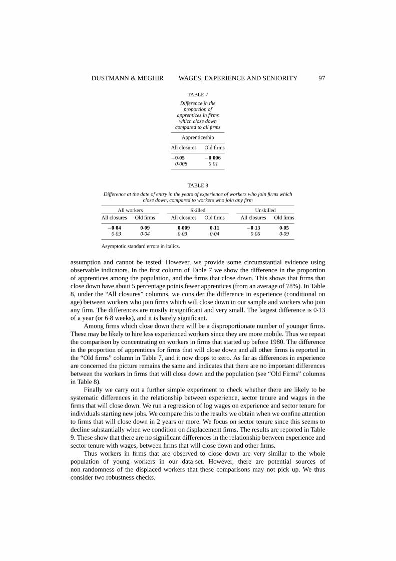
TABLE 7

Difference in theproportion of

apprentices in firmswhich close down

compared to all firms

Apprenticeship

All closures Old firms

−0·05 −0·0060·008 0·01

TABLE 8

Difference at the date of entry in the years of experience of workers who join firms whichclose down, compared to workers who join any firm

All workers Skilled UnskilledAll closures Old firms All closures Old firms All closures Old firms

−0·04 0·09 0·009 0·11 −0·13 0·050·03 0·04 0·03 0·04 0·06 0·09

Asymptotic standard errors in italics.

assumption and cannot be tested. However, we provide some circumstantial evidence usingobservable indicators. In the first column ofTable7 we show the difference in the proportionof apprentices among the population, and the firms that close down. This shows that firms thatclose down have about 5 percentage points fewer apprentices (from an average of 78%). InTable8, under the “All closures” columns, we consider the difference in experience (conditional onage) between workers who join firms which will close down in our sample and workers who joinany firm. The differences are mostly insignificant and very small. The largest difference is 0·13of a year (or 6·8 weeks), and it is barely significant.

Among firms which close down there will be a disproportionate number of younger firms.These may be likely to hire less experienced workers since they are more mobile. Thus we repeatthe comparison by concentrating on workers in firms that started up before 1980. The differencein the proportion of apprentices for firms that will close down and all other firms is reported inthe “Old firms” column inTable7, and it now drops to zero. As far as differences in experienceare concerned the picture remains the same and indicates that there are no important differencesbetween the workers in firms that will close down and the population (see “Old Firms” columnsin Table8).

Finally we carry out a further simple experiment to check whether there are likely to besystematic differences in the relationship between experience, sector tenure and wages in thefirms that will close down. We run a regression of log wages on experience and sector tenure forindividuals starting new jobs. We compare this to the results we obtain when we confine attentionto firms that will close down in 2 years or more. We focus on sector tenure since this seems todecline substantially when we condition on displacement firms. The results are reported inTable9. These show that there are no significant differences in the relationship between experience andsector tenure with wages, between firms that will close down and other firms.

Thus workers in firms that are observed to close down are very similar to the wholepopulation of young workers in our data-set. However, there are potential sources ofnon-randomness of the displaced workers that these comparisons may not pick up. We thusconsider two robustness checks.


TABLE 9

Relationship of experience and sector tenure to wages in the population of firms and the firmsthat will close down in2 years or more

Skilled UnskilledPopulation Firms that will close Population Firms that will close

Experience 0·0371 0·0502 0·050 0·07180·0007 0·0062 0·001 0·0102

Sector tenure 0·0116 0·0115 0·0164 0·01800·0006 0·0044 0·0016 0·0134

Asymptotic standard errors in italics.

The definition of the closure sample

In our data we know whether a firm closes down, independently of when the worker left, sincewe have direct access to a data-set reporting firm size over a 17 year period for any firm whichemployed any worker in our sample. Up to now we have defined the population of displacedworkers due to firm closure as the set of workers who left the firm which closed down within 1year of their departure. Using a narrow window to define a worker displaced due to closure makesit more likely that the worker is in fact displaced because of an imminent closure. On the otherhand, if the closure was anticipated by the management or by the worker, we may end up with aselected sample of workers (both in terms of observables and unobservables). This selection mayhave opposing effects: firms may lay off less productive workers first, or the best workers mayleave the firm before the closure. Taking a wider window mitigates this problem, but increasesthe risk that workers are included who moved for reasons other than closure.

In Table10 we present results for the returns to experience for the skilled and unskilledbased on the broader definition of closure. This defines as displaced any worker who left a firmthat closed down within 2 years of their departure. The number of displaced workers with thisdefinition increases from 3639 to 4589 for the skilled and from 1373 to 1796 for the unskilled.The regressions include the residuals, and they are comparable to the last column of Tables3(unskilled workers) and4 (skilled workers).

The estimated initial returns for the skilled and unskilled workers are lower now. However,the difference is insignificant with aP-value for this difference of 50% for the skilled and 58%for the unskilled. All other returns are very similar and overall the differences are completelyinsignificant.

In the first column ofTable11, we also report the results for firm tenure for this definition offirm closure. The returns to tenure for the first 5 years remain unchanged vis-a-vis our preferredresults in the last column ofTable6. The tenure returns beyond 5 years do increase but they arenot well determined.

Thus the results are not sensitive to the precise way of defining displaced workers, althoughif we estimate the model on all movers we get significantly different results, as shown in theprevious sections.

Is there evidence of bias due to self-selection by firm closure probability?

One reason that the closure sample may be non-random is that workers may self-select into firmsbased on any information relating to their closure probability. This assumption is important:workers with higher unobserved returns to tenure would avoid firms more likely to close down,since they suffer a larger loss from closure. This would lead to a downward bias in the estimatedaverage returns to tenure in the estimates we presented.


TABLE 10

Wage growth—experience, broader definitionof closure

Control function estimatorExperience Skilled Unskilled

One year — 0·073— 0·031

Two years 0·052 0·0740·017 0·032

Three years 0·056 0·0350·014 0·032

Four years 0·063 0·0390·016 0·029

Five years+ 0·010 −0·0040·004 0·010

No. obs. 4589 1796

Standard deviation of the block bootstrap initalics.

TABLE 11

Wage growth—tenure, unskilled and skilled, robustnesschecks

Tenure (years) Broad definition of closure Older firms

Skilled,<5 0·026 0·0150·0038 0·005

Skilled,≥5 0·026 0·00320·010 0·016

Unskilled,<5 0·040 0·0270·008 0·009

Unskilled,≥5 0·025 −0·0230·017 0·024

Standard deviation of the block bootstrap in italics.Control function estimator.

Our data provides information that allows us to present some evidence about this: as wehave seen, young firms are more likely to close down (seeFigure3). If workers with high returnsto tenure were trying to avoid firms with high closure probability they should avoid employmentin younger firms (all else being equal). Thus, we re-estimate our model based on the firms thatwere in existence before 1980 and subsequently closed down in our sample period. This leads toa drop in the sample of displaced workers by about 40%. If such self-selection was an importantphenomenon we should expect the returns to tenure to increase when using this sample, if indeedthe returns to tenure are heterogeneous.

The results on the returns to tenure using workers displaced from older firms are presentedin the second column ofTable11. These estimates show that the returns to tenure do not increasewhen using the sample of workers who were displaced following the closure of anolder firm;in fact they decrease. Hence from these results there is no indication that self-selection byprobability of closure has led to an underestimate of the returns to tenure. This reinforces ourview that the use of the displacement sample is a valid way to proceed. The returns to experienceare also similar and we do not report them for the sake of brevity.


5. CONCLUDING REMARKS

In this paper we analyse wage growth for workers in Germany. We focus on two groups: thosewith apprenticeship training (skilled workers) and those with no post-secondary school educationor formal training (unskilled workers).

The framework for our analysis is a model with match specific effects as well asheterogeneous returns to experience, firm tenure and sector tenure. We discuss a way ofidentifying and estimating this model based on displaced workers. The sample we consider isunique, in that we observe an accurate calendar of all job transitions from the beginning of theworkers’ careers. This has led us to consider workers up to the age of 35. As earlier studies haveshown, this is the period of the most rapid wage growth.

Wages of the skilled workers grow with experience and the profile is concave, with growthstarting at 7% early on, and falling to 1·2% a year beyond 4 years. The returns to staying in thesame sector are about 1% a year but they decline after 5 years, while the returns to staying in thesame firm are about 2·5% a year again declining after 5 years.

Wages of the unskilled workers only grow for the first 2–3 years of labour marketexperience. Experience related growth falls to zero following that. Their returns to sector tenureare close to zero and statistically insignificant. However, unskilled workers seem to benefit fromreturns to firm tenure which are about 4% a year for the first 5 years but decline to an insignificant1·1% thereafter. Thus, while the acquisition of transferable skills seems to be important for thewage growth of skilled workers early on in their career, unskilled workers benefit primarilyfrom being attached to a particular firm. An important implication of this is for the success oftemporary interventions in the labour market. Programmes that seek to improve employability ofthe unskilled via general work experience are likely to be less successful than programmes thatattempt to match a worker with a firm, possibly by an initial period of a job subsidy, at least inGermany.

APPENDIX A. THE SELECTION PROCESS INTO NEW JOBS

To see what the selection issue is and how exogenous displacements can help identify the returns to experience, we setup a mobility model for individuals. For the purpose of notational simplicity, we ignore here sector tenure, and we onlyconsider one education level; we therefore drop the indexa. Thus assume that individuals are risk neutral and denote byui f t the set of unobservablesmi f t , vi f t andηi t , wherei denotes individuals,f the firm or job, andt the time period. The

value of a job is denoted byV Jt (TG

it , T Fi f t , r t | ui f t ). At the start tenure is zero (T F

i f t = 0). We assume that a working

individual receives an alternative offer from a firmf ′. The value of unemploymentVUt (TG

it , wi l , di t | ηi t ) dependson benefitsBi t , which in general will depend on the previous wage (wi l ) and on unemployment duration (di t ). HenceBi t = Bi t (wi l , di t ). At the start of the unemployment spell duration will be zero.

Denote the value of the current job by

V Jt (TG

it , T Fi f t , r t | ui f t ) = wi f t + δEt max[V J

t+1(TGit + 1, T F

i f t + 1, r t+1 | ui f t+1),

V Jt+1(TG

it + 1, 0, r t+1 | ui f ′t+1), VUt+1l (TG

it + 1, wi l , 0, r t+1 | ηi t )],

whereδ is the discount factor andEt is the expectations operator conditional on information in periodt . The value ofunemployment is

VUt (TG

it , wi l , di t , r t | ηi t ) = Bi t + δEt max[V Jt+1(TG

it , 0, r t+1 | ui f ′′t+1), VUt+1(TG

it , wi l , di t + 1, r t+1 | ηi t )].

Expectations are taken over future realizations ofui f t andui f ′t conditional on the current value ofui f t and the otherstate variables (wheref and f ′ represent alternative firms).

Now consider the set of individuals observed starting a new job. They consist of two groups: first, those movingfrom an old job f to a new one f ′. Second, those who quit (or were layed off) in periods < t and have nowreceived an acceptable job offer. The former satisfy the conditionV J

t (TGit , 0, r t | ui f ′t ) > max{V J

t (TGit , T F

i f t , r t |

ui f t ), VUt (TG

it , wi f t , 0, r t | ηi t )} denoted for short byN J > 0. The latter satisfytwo conditionsVUs (TG

is , wis, 0, rs |

ηi t ) > max{V Js (TG

is , T Fi f s, rs | ui f s), V J

s (TGis , 0, rs | ui f ′s)} denoted byUs > 0 and V J

t (TGis , 0, r t | ui f t ) >


VUt (TG

is , wis, t − s, r t | ηi t ) denoted byN JU > 0. The latter group preferred unemployment to their previousjob and an alternative job offer; at durationt − s they obtained a job more acceptable than unemployment valued atdurationt − s.

Now consider the expected value of wages (lnwi f ) for individuals who start a new job in firmf , for a given level

of experience (TGit ) and for given value of the observable characteristicszi t .

E(ln wi f t | TGit , N Jt > 0 or [Us > 0 andN JU

t > 0], t, zi t )

= ln r t + [α + E(ηi t | TGit , N Jt > 0 or [Us > 0 andN JU

t > 0], t, zi t )]TGit

+ E(mi f t | TGit , N Jt > 0 or [Us > 0 andN JU

t > 0], t, zi t ). (A.1)

The expressionα + E(ηi t | TGit , [N Jt > 0 or [Us > 0 andN JU

t > 0]t, zi t ) is the average return to experience in

the population of those starting a new job, whileE(mi f t | TGit , N Jt > 0 or [Us > 0 andN JU

t > 0], t, zi t ) is theaverage match quality of these persons. The average return to experience which we want to estimate isα. However,modelling the dependence ofηi t and mi f t for new job starts is complicated by the fact that these individuals areselected by multiple ways; consequently this selection cannot be expressed by a single index as in theHeckman(1974)selection model. Now consider workers who are displaced for a completely exogenous reason. For them the selectionN Jt > 0 andUs > 0 are irrelevant. Consequently the selection terms become[α + E(ηi t | TG

it , N JUt > 0, t, zi t )]

and E(mi f t | TGit , N JU

t > 0, t, zi t ). The dependence of the conditional expectations onN JUt > 0 reflects the job

acceptance strategy of the unemployed and can be modelled as the standard selection into work, approximated by asingle index, as inHeckman(1974). The conditioning on experience (TG

it ) reflects the fact that the unobservables maybe serially correlated, and hence may affect past employment decisions and thus experience.

APPENDIX B. THE INSTITUTIONAL BACKGROUND IN GERMANY

Wage setting

Unlike the U.S., there is no general, government imposed minimum wage in Germany. Instead, there is an elaboratesystem of tariff contracts, which specify minimum wages according to occupation, sector, region and some personalcharacteristics. These minimum wages are determined by (annual) wage bargaining between unions and employerfederations (or single employers).

Bargaining takes place at industry and regional levels. Although in principle tariff agreements between an employer(or an employer association) and a union cover only employees who are union members, in practice the union status ofthe employee is irrelevant. The tariff contracts act as sector specific minimum wages for those firms that are membersof employer associations, or that negotiate directly with the union. Not all firms are bound to the tariff agreements,however. Firms which are not in the employer’s association do not have to pay tariff wages. In 1995, about 83% ofall workers were employed in firms that were bound by tariff agreements (seeDustmann and Schoenberg, 2002 fordetails).

Job security

The German dismissal regulations concern protection from dismissal, advanced notice, as well as severance payrequirements.

The general dismissal protection regulations foresee that all dismissals of employees who are employed for morethan 6 months without interruption, and which are initiated by the employer, are invalid if they are socially unacceptable.Dismissals must therefore be justified by the employer. Acceptable reasons for dismissal include rationalization,macroeconomic shocks, absenteeism, illness, etc.

The advanced notice period in Germany varies according to seniority and, before 1993, blue or a white collar statusof the worker. Furthermore, there may be particular industry regulations as well as firm–worker specific agreements. Ingeneral, the advanced notice regulations foresee 4 weeks of advanced notice for blue collar workers who have beenemployed for at least 5 years, and 12 weeks for white collar workers. After 20 years of employment with the samefirm, these periods rise to 12 weeks and 24 weeks for blue and white collar workers, respectively (seeButtler, Brandes,Dorndorf, Gaum and Walwei, 1992).

The education and apprenticeship system

The German Apprenticeship System (GAS) is a vocational training programme which combines on-the-job training,provided by the firm, with school education, provided by the state.


TABLE B1

Percentage working in each sector in our estimation data-set

Sector allocation

All Skilled Unskilled

Agriculture 1·80 1·72 2·10Energy, mining, water industry 2·62 2·45 3·21Chemical industry 7·21 6·93 8·23Metal industry, machines 13·83 14·09 12·88Electro technical industry, automobiles 13·38 14·19 10·37Optical industry, fine mechanics 3·81 3·51 4·91Wood, printing, paper 6·08 5·97 6·50Leather, textiles, food 5·36 5·23 5·83Construction, carpentry 12·65 12·53 13·07Trade 12·35 12·92 10·26Traffic, news 5·36 5·22 5·88Credit and insurance 2·72 3·23 0·86Services 7·82 7·04 10·71Charities 1·79 1·76 1·94Public services 3·22 3·21 3·23

Total 100·00 100·00 100·00

TABLE B2

Log wages and job number, Germany IAB

Number of job Unskilled Skilled

Coeff t ratio Coeff t ratio

2 0·0277 6·574 −0·0188 −11·4733 0·0014 0·290 −0·0437 −21·3674 −0·0419 −7·016 −0·0795 −30·6205 −0·0730 −10·310 −0·1003 −29·1406 −0·1067 −12·714 −0·1206 −26·7227 −0·1371 −13·526 −0·1624 −26·9408 −0·1841 −15·277 −0·2325 −29·601

All regressions include age and time dummies.

The roots of the apprenticeship system can be traced back to the Middle Ages, when the craft guilds regulatedjourneymanship type training schemes, and issued training certificates. Today, more than 60% of each cohort in Germanygoes through the apprenticeship system (seeSoskice, 1994). In 1990, there were about 370 recognized apprenticeshipoccupations. These occupations include both blue and white collar professions, and cover many professions which requirecollege attendance in the U.K. and the U.S. (as, for instance, accountancy etc.).

Apprenticeship training schemes last between 2 and 3·5 years. During this time, apprentices attend on average 1–2days a week a vocational state school, where they acquire general knowledge, as well as knowledge which is specific totheir occupation. For the remaining days, they are on on-the-job training schemes within the firm. Qualified personnelis responsible for the apprentice, and allocates apprentices to particular tasks. Larger firms run also specific classes orseminars for apprentices.

APPENDIX C. SECTOR EMPLOYMENT ALLOCATION, JOB MOBILITY, WAGES ANDWAGE GROWTH

The following are regressions of log wages on job number, age dummies, and time dummies for Germany and the U.S.TableB2 does not include fixed effects;TableC1does include fixed effects.


TABLE C1

Log wages and job number, Germany IAB, fixed effects

Number of job Unskilled Skilled

Coeff t ratio Coeff t ratio

2 0·1292 29·473 0·0611 37·386

3 0·1542 28·327 0·0821 38·689

4 0·1580 24·219 0·0817 30·597

5 0·1434 18·965 0·0861 25·834

6 0·1297 14·835 0·0843 20·327

7 0·1220 12·025 0·0646 12·443

8 0·1017 8·727 0·0228 3·531

All regressions include age and time dummies.

TABLE C2

Impact of residuals on the wage equation with selectioncorrection—displaced sample

Experience Tenure

Coeff StdE Coeff StdE

υ P−0·022 0·0370 −0·036 0·0032

υ P× c 0·0179 0·0066 0·0198 0·006

υ P× TG

−0·0012 0·012 −0·014 0·0081

υ P× TG

× c −0·0010 0·0011 −0·00002 0·0008

υ P× T S

−0·0116 0·0087 −0·0021 0·0075

υ P× T S

× c 0·0010 0·0009 −0·0004 0·0008

υ P× T F

−0·013 0·018

υ P× T F

× c 0·00022 0·0016

υG−0·0315 0·0162 −0·035 0·0152

υG× c 0·0024 0·0017 0·0059 0·0020

υG× TG 0·0090 0·0038 0·0057 0·0035

υG× TG

× c −0·0004 0·0003 −0·0004 0·0003

υG× T S 0·0028 0·0037 0·0021 0·034

υG× T S

× c −0·0003 0·0003 −0·0002 0·0003

υG× T F 0·0054 0·0076

υG× T F

× c −0·0010 0·0006

υT 0·0070 0·0055

υT× c −0·0052 0·0021

υT× TG 0·0001 0·0026

υT× TG

× c 0·0005 0·0002

υT× T S 0·0024 0·0013

υT× T S

× c −0·00014 0·00013

υT× T F

−0·011 0·0035

υT× T F

× c 0·00082 0·00027

P-value for joint sign. 0% 0%

Bootstrap standard errors (StdE) and critical values. 200 replications used

Notation Equation (6) Equations (9)–(12)


APPENDIX D. THE REDUCED FORM RESULTS AND THE COEFFICIENTS OF THERESIDUALS

TABLE D1

Cell sizes by experience for the displaced sample

Cell size in post-displacement recordsFirst job record

Experience Skilled Unskilled

0 — 3391 — 2162 448 1853 931 1484 611 1285 397 756 334 677 253 498+ 663 122

For skilled workers experience includes timespent in apprenticeship. We observe skilledworkers once apprenticeship is over. The levelof experience at which we first observe themdepends on the length of apprenticeship.

TABLE D2

Reduced forms, unskilled workers

Participation Experience Tenure

Coeff StdE Coeff StdE Coeff StdE

Age 0·0425 0·0060 0·217 0·077 0·388 0·079ci t 0·678 0·0247 0·5635 0·0604 0·439 0·064ci t × age −0·019 0·0007 −0·0071 0·0039 −0·018 0·004Lower secondary 0·1550 0·0143 0·5357 0·1220 0·38 0·094School unknown 0·0172 0·0165 −0·1899 0·1382 −0·63 0·108Age 18 0·0124 0·0126 −0·3428 0·1030 −0·568 0·105Age 19 −0·0072 0·0171 −0·6038 0·1805 −0·972 0·184Age 20 0·1082 0·0239 −1·05 0·2593 −1·50 0·263Age 21 0·0673 0·030 −1·291 0·3391 −1·78 0·344Age 22 0·1192 0·0373 −1·890 0·4154 −2·20 0·426Age 23 0·1273 0·0433 −2·329 0·493 −2·61 0·510Age 24 0·099 0·0497 −2·851 0·5723 −2·98 0·592Age 25 0·1363 0·0565 −3·430 0·6528 −3·46 0·684Age 26 0·1002 0·0625 −4·026 0·7337 −3·66 0·77Age 27 0·1254 0·0700 −4·499 0·8156 −3·96 0·873Age 28 0·0523 0·0772 −4·968 0·9008 −4·18 0·982Age 29 0·028 0·0852 −5·278 0·9920 −4·21 1·06Age 30 0·0013 0·092 −4·675 1·065 −3·25 1·1Age 31 0·0007 0·1040 −3·947 1·146 −2·1 1·12Age 32 0·1835 0·1124 −1·65 1·225 0·651 1·38Age 33 0·0455 0·143 −0·6215 1·250 0·828 1·55Age 34 −0·2497 0·1669 −0·2204 1·08 0·409 1·54ci t × age 18 −0·1358 0·0127 0·1785 0·0223 0·209 0·024ci t × age 19 −0·1761 0·0116 0·2525 0·0255 0·241 0·028ci t × age 20 −0·242 0·0116 0·3666 0·0297 0·31 0·031


TABLE D2—Continued

Reduced forms, unskilled workers



ci t × age 21 −0·2312 0·0108 0·3541 0·0336 0·289 0·035ci t × age 22 −0·2289 0·0101 0·4274 0·0363 0·311 0·039ci t × age 23 −0·2142 0·0096 0·459 0·0400 0·334 0·044ci t × age 24 −0·1950 0·0091 0·5014 0·0435 0·356 0·047ci t × age 25 −0·1850 0·0086 0·5446 0·0475 0·399 0·053ci t × age 26 −0·163 0·0083 0·5740 0·0516 0·396 0·058ci t × age 27 −0·1488 0·008 0·5885 0·0560 0·411 0·063ci t × age 28 −0·1242 0·0077 0·6074 0·0605 0·413 0·069ci t × age 29 −0·1060 0·0076 0·6091 0·0649 0·40 0·072ci t × age 30 −0·0866 0·0076 0·5282 0·0680 0·306 0·077ci t × age 31 −0·0706 0·0078 0·432 0·0715 0·202 0·07ci t × age 32 −0·0657 0·0078 0·2288 0·0763 −0·015 0·087ci t × age 33 −0·039 0·0095 0·1208 0·0766 −0·035 0·092ci t × age 34 −0·0020 0·0104 0·0375 0·0647 −0·020 0·093

Observations 47,998 47,998 55,882R-squared 0·16 0·77 0·28P-value for age dummies 0·00 0·00 0·00

P-value for age dummies× ci t 0·0 0·0 0·0

StdE are standard errors allowing for heteroscedasticity and serial correlation. Default educationgroup: Higher Secondary. Youngest age is 16. All regressions include time dummies. Experienceand tenure are measured in years including fractions of a year; Participation is measured infractions of a year worked. The number of observations include non-work spells in the case ofexperience and tenure. For tenure there may be multiple records per year.

TABLE D3

Reduced forms, skilled workers



Age 0·0173 0·0039 0·433 0·0593 0·314 0·077ci t −0·0102 0·0507 1·55 0·0963 −0·409 0·2064ci t × age −0·0000 0·0014 −0·036 0·0043 0·007 0·0072Lower secondary 0·012 0·0052 0·355 0·0592 0·44 0·087School unknown −0·1069 0·0073 −0·095 0·0698 −1·2 0·097Age 20 −0·1272 0·0251 −0·428 0·0655 −0·569 0·1230Age 21 −0·1767 0·0246 −0·846 0·1223 −0·896 0·1802Age 22 −0·2004 0·0246 −1·32 0·1808 −1·33 0·2487Age 23 −0·1777 0·0257 −1·82 0·2397 −1·74 0·3218Age 24 −0·1255 0·0273 −2·29 0·2988 −2·07 0·3976Age 25 −0·1021 0·0296 −2·72 0·3580 −2·29 0·4752Age 26 −0·1152 0·0320 −3·17 0·4165 −2·56 0·5528Age 27 −0·1053 0·0349 −3·61 0·4756 −2·81 0·6325Age 28 −0·095 0·0380 −4·07 0·5341 −3·19 0·7129Age 29 −0·0981 0·0419 −4·43 0·5945 −2·98 0·7931Age 30 −0·0680 0·0455 −4·70 0·6517 −1·82 0·8746Age 31 −0·0783 0·0494 −4·96 0·7068 −1·21 0·9477Age 32 −0·0747 0·0521 −5·16 0·7615 −0·815 1·02Age 33 −0·1559 0·0633 −4·70 0·798 −0·948 1·038Age 34 −0·1476 0·067 −3·13 0·7177 −1·17 0·947


TABLE D3—Continued

Participation Experience TenureCoeff StdE Coeff StdE Coeff StdE

ci t × age 20 0·0420 0·0220 −0·007 0·02 0·40 0·0802ci t × age 21 0·0404 0·0206 −0·034 0·0246 0·43 0·0755ci t × age 22 0·0518 0·0190 −0·015 0·0247 0·473 0·0710ci t × age 23 0·0428 0·0176 0·040 0·0255 0·511 0·0673ci t × age 24 0·0263 0·016 0·087 0·0269 0·525 0·0644ci t × age 25 0·0197 0·0147 0·128 0·0290 0·515 0·0625ci t × age 26 0·0203 0·0133 0·172 0·0314 0·51 0·0610ci t × age 27 0·0177 0·0119 0·220 0·0343 0·519 0·0607ci t × age 28 0·0150 0·0106 0·266 0·0373 0·529 0·0612ci t × age 29 0·0140 0·0093 0·299 0·0409 0·468 0·0628ci t × age 30 0·0101 0·0080 0·322 0·0443 0·308 0·065ci t × age 31 0·0095 0·0068 0·345 0·0476 0·207 0·0670ci t × age 32 0·0086 0·0057 0·369 0·0509 0·154 0·0707ci t × age 33 0·0136 0·0053 0·333 0·0531 0·14 0·0699ci t × age 34 0·0116 0·004 0·219 0·0476 0·122 0·0626

Observations 181,206 181,206 204,503R-squared 0·067 0·83 0·14P-value for age dummies 0·0 0·0 0·0P-value for age dummies× ci t 0·0 0·0 0·0

Youngest age is 17. Other notes as inTableD2 for unskilled workers.

TABLE D4

Results including a quadratic term—control function estimator—post-displacement

Experience Sector tenure Tenure

Skilled Unskilled Skilled Unskilled Skilled Unskilled

One year 0·102 ≤5 years 0·0097 −0·015 0·032 0·0680·034 0·0079 0·019 0·011 0·017

Two year 0·083 0·084 >5 years 0·007 −0·063 0·032 0·110·021 0·038 0·032 0·079 0·023 0·047

Three years 0·083 0·033 Tenure2 −0·00002 0·0048 −0·0020 −0·00800·018 0·042 0·0019 0·0046 0·0025 0·0036

Four years 0·076 0·0400·020 0·050

Five years+ 0·058 −0·0070·028 0·057

Experience2 −0·0029 −0·00040·0017 0·0035

P-value∗ 0·26 0·51 0·085

Standard deviation of the block bootstrap in italics.∗ P-value corresponds to the two degree of freedom testfor excluding the quadratic terms in each part of the model.P-value of joint six degrees of freedom test forexcluding all quadratic terms is 0·18. Experience, tenure and sector tenure measured in years.

Acknowledgements. We thank three anonymous referees and the editor James Dow for useful comments andsuggestions. Discussions with Joe Altonji, Orazio Attanasio, James Banks, Richard Blundell, Ken Burdett, LorraineDearden, Jim Heckman, Derek Neal, Gillian Paull, Jean-Mark Robin, Uta Schoenberg, Chris Taber and Yoram Weissproved particularly useful in developing this paper. We would also like to thank participants in seminars at the Universitiesof Aarhus (Denmark), Chicago, Copenhagen, Essex (U.K.), IIES (Sweden), Northwestern, Pennsylvania, Pompeu Fabra(Barcelona), as well as the EUI (Florence) and ECARE (Brussels), for stimulating comments. We thank the ESRC centrefor the analysis of Fiscal Policy at the IFS and the Anglo German foundation for funding the project. We also thank theIAB for letting us use the data and Stefan Bender for his invaluable help with it. We remain responsible for all errors andinterpretations.


REFERENCES

ALTONJI, J. G. and SHAKOTKO, R. A. (1987), “Do Wages Rise with Seniority?”,Review of Economic Studies, 54,437–459.

ALTONJI, J. G. and WILLIAMS, N. (1996), “The Effects of Labor Market Experience, Job Seniority and Job Mobilityon Wage Growth” (Mimeo).

ALTONJI, J. G. and WILLIAMS, N. (1997), “Do Wages Rise with Seniority? A Reassessment” (Mimeo).BECKER, G. (1993)Human Capital(NBER, The Chicago University Press).BENDER, S., DUSTMANN, C., MARGOLIS, D. and MEGHIR, C. (2002), “Worker Displacement in France and

Germany, in Loosing Work, Moving On”, in P. J. Kuhn (ed.) (Michigan: Upjohn Institute) 375–452.BENDER, S., HILZENDEGEN, J., ROHWER, G. and RUDOLPH, H. (1996), “Die IAB Beshaeftigungsstichprobe

1975–1990”,Beitraege zur Arbeitsmarkt- und Berufsforschung, BeitrAB 197, Nurnberg.BEN-PORATH, Y. (1967), “The Production of Human Capital and the Life Cycle of Earnings”,Journal of Political

Economy, 75, 352–365.BJORKLUND, A. and MOFFITT, R. (1987), “The Estimation of Wage Gains and Welfare Gains in Self-Selection”,

Review of Economics and Statistics, 69, 42–49.BLINDER, A. and WEISS, Y. (1976), “Human Capital and Labor Supply: A Synthesis”,Journal of Political Economy,

84 (3), 449–472.BURDA, M. and MERTENS, A. (2001), “Wages and Worker Displacement in Germany”,Labour Economics, 8, 15–41.BUTTLER, F., BRANDES, W., DORNDORF, E., GAUM, W. and WALWEI, U. (1992), “Flexibility and Job Security in

the Federal Republic of Germany”, Technical Report 1, SAM (Working Paper).CARD, D. (2001), “Estimating the Returns to Schooling: Progress on some Persistent Econometric Problems”,

Econometrica, 69, 1127–1160.DATTA, S. (1995), “Building Trust” (Mimeo, LSE).DUSTMANN, C. and SCHOENBERG, U. (2002), “Training and Unions” (Mimeo, UCL).ECKSTEIN, Z. and WOLPIN, K. (1989), “Dynamic Labour Force Participation of Married Women and Endogenous

Work Experience”,Review of Economic Studies, 56 (3).FARBER, H. S. (1983), “The Determination of the Union Status of Workers”,Econometrica, 51 (5), 1417–1438.FARBER, H. S. (1994), “The Analysis of Interfirm Worker Mobility”,Journal of Labor Economics, 12, 554–593.FITZENBERGER, B. and KURZ, C. (2003), “New Insights on Earnings Trends Across Skill Groups and Industries in

West Germany”,Empirical Economics, 28 (3), 479–513.FLORENS, J. P., HECKMAN, J. J., MEGHIR, C. and VYTLACIL, E. (2002), “Instrumental Variables, Local

Instrumental Variables and Control Functions” (Mimeo, UCL/IFS).GAREN, J. (1984), “The Returns to Schooling: A Selectivity Bias Approach with Continuous Choice Variables”,

Econometrica, 52, 1199–1218.GIBBONS, R. and KATZ, L. (1992), “Does Unmeasured Ability Explain Inter-industry Wage Differentials?”,Review of

Economic Studies, 59, 515–535.HALL, P. and HOROWITZ, J. (1996), “Bootstrap Critical Values for Tests Based on Generalized-Method-of-Moments

Estimators”,Econometrica, 64 (4), 891–916.HARRIS, C. and FELLI, L. (1996), “Learning, Wage Dynamics, and Firm Specific Human Capital”,Journal of Political

Economy, 104, 838–868.HASHIMOTO, M. (1981), “Firm Specific Human Capital as a Shared Investment”,American Economic Review, 71 (3),

475–482.HECKMAN, J. J. (1974), “Shadow Prices, Market Wages, and Labor Supply”,Econometrica, 42, 679–694.HECKMAN, J. J. (1979), “Selection Bias as a Specification Error”,Econometrica, 47, 153–162.HECKMAN, J. J. (1995), “Instrumental Variables: A Cautionary Tale” (Mimeo).HECKMAN, J. J. and ROBB, R. (1985), “Alternative Methods for Evaluating the Impact of Interventions”,

in J. J. Heckman and B. Singer (eds.)Longitudinal Analysis of Labor Market Data Econometric Society MonographSeries No. 10(Cambridge University Press) 156–245.

HECKMAN, J. J. and SEDLACEK, G. (1985), “Heterogeneity, Aggregation and Market Wage Functions: An EmpiricalModel of Self-Selection in the Labor Market”,Journal of Political Economy, 93 (6), 1077–1125.

HECKMAN, J. J. and VYTLACIL, E. (1998), “Instrumental Variables Methods for the Correlated RandomCoefficient Model: Estimating the Average Rate of Return to Schooling When the Return is Correlated withSchooling” (Mimeo, University of Chicago).

HOROWITZ, J. (2001), “The Bootstrap”, in J. J. Heckman and E. Leamer (eds.)The Handbook of Econometrics, Vol. 5,(Amsterdam: North-Holland).

IMBENS, G. W. and ANGRIST, J. D. (1994), “Identification and Estimation of Local Average Treatment Effects”,Econometrica, 62 (2), 467–475.

JOVANOVIC, B. (1979), “Firm Specific Capital and Turnover”,Journal of Political Economy, 87, 1246–1260.KILLINGSWORTH, M. (1982), “Learning by Doing and Investment in Training: A Synthesis of Two Rival Models of

the Life Cycle”,Review of Economic Studies, 49, 263–271.KLETZER, L. G. (1989), “Returns to Seniority after Permanent Job Loss”,American Economic Review, 79 (3), 536–543.NAGYPAL, E. (2002), “Learning by Doing Versus Learning about Match Quality: Can we Tell them Apart?” (Mimeo,

Northwestern University and University of Stockholm).


NEAL, D. (1995), “Industry-Specific Human Capital: Evidence from Displaced Workers”,Journal of Labor Economics,13, 653–677.

NEWEY, W. , POWELL, J. and VELLA, F. (1999), “Nonparametric Estimation of Triangular Simultaneous EquationsModels”,Econometrica, 67, 565–604.

PARENT, D. (1995), “Industry-Specific Capital and the Wage Profile: Evidence from the NLSY and the PSID” (WorkingPaper No. 795, Universite de Montreal, Centre de Recherche et Developement en Economique).

ROBIN, J. M. and SMITH, R. (2000), “Tests of Rank”,Econometric Theory, 16, 151–175.ROSEN, S. (1972), “Learning and Experience in the Labor Market”,Journal of Human Resources, 7, 336–342.ROSEN, S. (1976), “A Theory of Life Earnings”,The Journal of Political Economy, 84 (4) Part 2: Essays in

Labor Economics in Honor of H. Gregg Lewis, S45–S67.SCOONES, D. and BERNHARDT, D. (1996), “Promotion Turnover and Discretionary Human Capital Acquisition”

(Mimeo).SOSKICE, D. (1994), “Reconciling Markets and Institutions: The German Apprenticeship System”, in L. Lynch (ed.)

Training and the Private Sector—International Comparisons(Chicago: University of Chicago Press for NBER).TOPEL, R. H. (1991), “Specific Capital, Mobility and Wages: Wages Rise with Job Seniority”,Journal of Political

Economy, 99, 145–176.TOPEL, R. H. and WARD, M. P. (1992), “Job Mobility and the Careers of Young Men”,Quarterly Journal of Economics,

107, 439–479.WILLIS, R. and ROSEN, S. (1979), “Education and Self-Selection”,Journal of Political Economy, 87(5) Part 2, S7–S36.

wages, experience and seniority - ucl - london's global …uctpb21/cpapers/wagesexpsen.pdf ·...

Documents