wage rigidity and labor market dynamics with sorting - iza · wage rigidity and labor market...
TRANSCRIPT

Wage Rigidity and Labor MarketDynamics with Sorting∗
Bastian Schulz†
University of Munich and Ifo Institute
May 7, 2015
Abstract
This paper adds two-sided ex-ante heterogeneity and a production technology induc-ing sorting to the canonical Diamond-Mortensen-Pissarides (DMP) search and matchingmodel. Ex-ante heterogeneity and sorting have important implications for the dynamicproperties of the model. The modifications solve the problem that standard DMP modelsdo not generate enough volatility in response to shocks, also known as the “Shimer Puzzle”(Shimer, 2005). Amplification to overcome the volatility puzzle stems from an endoge-nously generated wage rigidity, which is of reasonable magnitude given empirical evidencefrom the U.S. labor market. Additionally, endogenous matching sets fluctuate in responseto shocks and amplify job-creation. Using a standard Nash sharing rule, I show that thesurplus function of the model, which depends on both workers’ and firms’ outside options,exhibits an asymmetry in equilibrium that stems from unequal bargaining powers. Usingthe standard calibration of the model, the firms’ matching sets are wider in equilibriumthan the workers’ matching sets and fluctuate more in response to shocks.
Keywords: Sorting, Mismatch, Wage Rigidity, Heterogeneity, Unemployment, Search and
Matching, Aggregate Fluctuations
JEL Classifications: E24, E32, J63, J64
∗ I would like to express my gratitude to Helmut Rainer and Christian Holzner for many invalu-able suggestions and their general support and encouragement. This paper benefited from use-ful discussions with Wouter den Haan, Philipp Kircher, Rasmus Lentz, Christian Merkl, NicolasPetrosky-Nadeau, Jean-Marc Robin, Uwe Sunde, and Joanna Tyrowicz. Comments from seminarand conference participants at LMU Munich, FAU Erlangen-Nuremberg, IAB Nuremberg, SMYE2014 (Vienna), the 2014 European Winter Meeting of the Econometric Society (Madrid), the 2015Annual Meeting of the AEA (Boston), T2M 2015 (Berlin), and the 2015 Annual Conference of theRES (Manchester) are highly appreciated. I am solely responsible for all remaining errors.
† Contact: Ifo Institute - Leibniz Institute for Economic Research at the University of Munich, IfoCenter for Labour Market Research and Family Economics, Poschingerstrasse 5, 81679 Munich,Germany, Phone: +49 (0)89 9224 1207, E-mail: [email protected]
1

1 Introduction
A large literature in labor economics shows how frictions and information imperfections
prevent labor markets from clearing. This explains the existence of equilibrium unem-
ployment. Job seekers and employers have to spend time and money to locate a suitable
counterpart and negotiate before eventually forming a match and starting production.
This coordination friction can be understood as an outcome of heterogeneity. Workers
and firms differ, for instance, with respect to their location or the supply and demand of
specific skills, which makes finding a suitable partner and forming a match costly. This
is the essence of the Diamond-Mortensen-Pissarides (DMP) search and matching frame-
work. It incorporates the coordination friction elegantly without making heterogeneity
across workers and firms explicit.1 In this class of models, the wage is determined by
simple Nash bargaining. Shimer (2005) points out that it is due to this sharing rule that
a simple dynamic DMP model largely fails to generate sufficient volatility in response to
aggregate shocks. He argues that this shortcoming, also known as the “Shimer Puzzle”,
has a distinct connection to the wage formation mechanism. Cyclical fluctuations in the
value of unemployment, which is the worker’s outside option, are absorbed entirely by
the fully-flexible wage. This reduces the incentive to create new jobs on the firm side,
thereby limiting the overall responsiveness of the model to shocks. Many papers show, in
turn, that this volatility puzzle can be solved by making wages less responsive to shocks,
either by simply assuming rigid wages (Hall (2005)), by modifying the calibration to
increase the worker’s outside option (Hagedorn and Manovskii (2008)), or by replacing
the Nash sharing rule with a more credible bargaining game (Hall and Milgrom (2008)).2
The model I propose in this paper solves this problem in a new way. It generates rigid
wages endogenously while sticking to the simple Nash sharing rule at the same time.
This property arises as a result of explicit heterogeneity across workers and firms. I as-
sume complementarity of types in production and, hence, positive assortative matching.
This modification enables the model to overcome the Shimer Puzzle via adjustments of
both the wage-formation mechanism and the firms’ job-creation condition. In the light
of recent advances and new insights into empirically identifying the sign and strength
1 In the baseline DMP model, the arrival of suitable match opportunities is governed by a Poissonprocess which depends on the aggregate state of the labor market. In the dynamic setting, repre-sentative workers and firms base their optimal, forward-looking decisions solely on the expected lawof motion of this aggregate state, which is the tightness of the labor market, defined as job-openingsper unemployed worker.
2 The volatility puzzle itself and approaches to solve it are still highly debated. Hornstein et al. (2005)and other papers discuss the modifications necessary to align the standard search and matchingmodel with the data from the perspective of empirical plausibility.
2

of sorting in labor market data (Gautier and Teulings (2006), Andrews et al. (2008),
Lopes de Melo (2009), Eeckhout and Kircher (2011), Hagedorn et al. (2012), Bartolucci
and Devicienti (2013), Bagger and Lentz (2014)), the model provides a both micro-
founded and empirically supported complement to existing approaches to better align
search and matching models with the data.
My equilibrium framework is inspired by Hagedorn et al. (2012). Sorting makes the
allocation of workers to jobs meaningful, both in terms of match-specific output and over-
all welfare. It implies that an optimal counterpart exists for every market participant.
In the absence of labor market frictions, a firm (worker) would instantaneously match
with the optimal employee (employer). This would lead to the Walrasian first-best al-
location, just like in Gary Becker’s neoclassical marriage market model (Becker (1973)).
Due to frictions and costly search, however, this optimal, welfare-maximizing allocation
of workers to jobs can never be realized. As shown by Shimer and Smith (2000), an
equilibrium property in this class of models is that workers and firms are picky, that is,
they are willing to match only with a subset of types in the vicinity of their optimal
counterpart. The cardinality of these so-called matching sets depends on the degree of
complementarity in production. The matching sets are endogenously determined and
have important implications for the dynamics of the model. They directly influence both
the values of being unemployed and maintaining an unfilled vacancy which are, in turn,
the outside options in the Nash bargaining solution.
This paper is, to the best of my knowledge, one of the first two that consider business
cycle fluctuations in a search and matching model with two-sided ex-ante heterogeneity
and sorting. The other, Lise and Robin (2014), builds on Postel-Vinay and Robin
(2002) and Robin (2011) to show that a model with on-the-job search and aggregate
uncertainty matches the data well, also with respect to unemployment fluctuations. The
key difference to my model is that the main theoretical result of Lise and Robin (2014)
does not hold with a Nash sharing rule. In my model, the surplus function depends
not only on the current state of the aggregate shock (as in Lise and Robin (2014)) but
additionally on the agents’ outside options which are functions on the matching sets.
This leads to richer dynamics via two channels: The matching sets fluctuate in response
to shocks and constitute an additional margin of adjustment in the dynamic job-creation
condition. Additionally, the surplus function exhibits the following interesting property:
unequal bargaining powers lead to an asymmetry between the outside options of workers
and firms in equilibrium. Since workers typically get a larger share of the surplus in the
standard calibration of search and matching models, firms’ matching sets are wider in
3

equilibrium and more volatile in response to shocks. In the wage equation, this appears
as a relative, i.e. match-specific labor market tightness term which is on average lower
than aggregate labor market tightness. This property shields match-specific wages from
fluctuations of the outside option and, thus, generates a real rigidity.
To solely focus on the consequences of sorting for the dynamics of the model and
analyze them transparently, I stick to most of the standard model’s assumptions. Thus,
I also abstract from search on the job. While this is without doubt a strong assumption,
I argue that search on the job would not alter the conclusions I draw and, hence, can
be left aside for the sake of clarity. On-the-job search takes effect in this class of mod-
els simply by relaxing the agents’ pickiness. This is due to the possibility of continued
search after matching with a non-optimal partner. The degree of pickiness, however, can
be controlled by the degree of complementarity in production. I can thus analyze the
influence of different degrees of pickiness in my model without the additional layer of
complexity that search on the job would add. This allows me to analyze the mechanism
behind the amplification I find as transparent as possible. For the same reason, I cali-
brate the model along the lines of Shimer (2005) for the U.S. labor market to conduct
numerical simulations under aggregate uncertainty. My results are therefore directly
comparable to both previous work on the dynamics of DMP models and the wider field
of macroeconomic models with frictional labor markets. In fact, the link is so close that
the model can be reduced to the well-known textbook version of the basic DMP model
simply by collapsing the type space into a single point.3
The wage rigidity, my main finding, arises solely out of equilibrium properties of the
search and matching model with sorting: I consider positive sorting based on both
absolute and comparative advantage and show that the augmented model creates an
elasticity of wages with respect to labor productivity of less than unity in both cases.
This implies that wages do not fully adjust and do not follow labor productivity one-
to-one as in the standard model. I find a moderate and empirically plausible elasticity
of 0.75 (absolute advantage) and 0.87 (comparative advantage). These elasticities are
close to the benchmark estimates for the U.S. labor market reported by Haefke et al.
(2013), who find an elasticity of 0.8 with a standard error of 0.4. The moderate rigidity
alone, however, does not generate sufficient amplification to overcome Shimer’s volatility
puzzle. I show that the second adjustment of the model with sorting, the modified job-
creation condition, is the main source of additional volatility in response to shocks.
3 I use a series or robustness checks to show that the simplifying assumptions do not induce anyloss of generality with respect to the key mechanism at the core of the augmented model. Theabstraction from search on-the-job is also further discussed in Section 4.
4
Firms’ expected surplus changes along two margins: First, in response to a positive
shock the surplus function shifts upwards. Second, additional workers with positive
surplus enter the equation due to wider matching sets. Therefore, a higher number
of additional vacancy postings is the optimal response to a positive shock. I conclude
that a simple dynamic DMP model with heterogeneity and sorting does not need any
additional modifications to generate rigid wages and amplification. The DMP model’s
volatility problem vanishes with sorting. In the presence of aggregate uncertainty, two
channels contribute to the amplification effect: the endogenously generated wage rigidity
and the effect of sorting on the forward-looking job creation decision.
The remainder of this paper is structured as follows: Section 2 develops the model and
derives the wage-formation mechanism in the presence of heterogeneous agents and sort-
ing as a bargaining outcome in the recursive framework. The equilibrium is characterized
and the computational strategy is briefly outlined. Section 3 presents numerical simula-
tions under aggregate uncertainty and compares the results of the augmented model to
the baseline model in the light of empirical moments from the U.S. labor market data.
The interplay between sorting, wage formation, and the model’s dynamics is analyzed
in more detail and robustness checks are presented. Section 4 discusses the results in
the light of related theoretical and empirical literature. Section 5 concludes.
2 The Model
2.1 Setup
I construct a fully dynamic two-sided equilibrium search and matching model with dis-
counting and transferable utility. Workers and firms are heterogeneous. Uncertainty
with respect to worker and firm types is not considered, that is, agents know their own
type and the types of all possible matching partners. Time is discrete. Workers and
firms are risk neutral, infinitely lived, and seek to maximize their expected discounted
future income streams. The parameter β represents the common discount factor. As in
the canonical search and matching model, only unemployed individuals search randomly
in this model; employed workers do not search. In case of unemployment, workers re-
ceive constant unemployment benefits b every period, which can also be interpreted as
the value of non-market activity. Vacant firms have to pay per-period vacancy post-
ing costs κ, representing expenses for posting vacancies, screening applications, and so
forth. Productive activity commences when a firm and a worker who meet in the la-
5
bor market are able to jointly produce a non-negative surplus given their types. If this
is the case, the surplus is shared according to the standard Nash bargaining solution
with workers having bargaining power α. Every period, matches between firms and
workers may terminate for two possible reasons: One the one hand, they are subject to
idiosyncratic separation shocks, which lead to immediate dissolution of the employment
relationship. These shocks hit a match with an exogenous per-period probability δ. On
the other hand, in the presence of aggregate uncertainty and business cycle fluctuations,
the model allows for endogenous separations, which may occur at the margins of the
agents’ matching sets. When a negative productivity shock hits the economy, the sur-
plus of previously marginally profitable employment relationships may become negative.
Since a negative surplus is always less than both parties’ outside option, they prefer to
separate. This mechanism is in line with Mortensen and Pissarides (1994) only that in
my model, aggregate rather than idiosyncratic productivity shocks trigger separations.
2.2 The Type Space
Following Shimer and Smith (2000), I assume atomless distributions of both worker and
firm types. The population of infinitely-lived agents is constant, that is, the model is
stationary. Workers are endowed with heterogeneous skills, indexed by s, and firms differ
from each other in terms of job complexity, indexed by c. Both skills and job complexity
can be viewed as a one-dimensional representation of a larger, multi-dimensional set of
worker and firm characteristics. I assume that both firms and workers can be unam-
biguously ranked based on skills and job complexity.4 Skills, s, and job complexity, c,
are distributed uniformly on the open interval. The overall probability density function
for workers and firms are time constant, normalized to 1, and denoted by, gw(s) and
gf (c). Table 1 shows how these densities relate to the distribution of unemployed work-
ers of type s, gu(s), and the distribution of vacant firms of type c, gv(c), which are both
equilibrium objects that vary over time in the presence of aggregate uncertainty. They
entail the probability of meeting a specific worker or firm type. The aggregate number
of vacancies, V , and unemployed workers, U , are computed by taking the integral over
the distribution of vacant firms or unemployed workers, respectively. gm(s, c) is the two-
dimensional distribution of active matches. The integral over either dimension yields the
probability distributions of employed workers, ge(s), and producing firms, gp(c). The
4 In an empirical setting, constructing such a ranking given the available matched employer-employeedata is indeed the most difficult part of identifying the sign and the strength of sorting, see alsothe discussions in Eeckhout and Kircher (2011) and Hagedorn et al. (2012).
6

Table 1: Labor market states, density and distribution functions, andaggregation
Description Density/Distribution Function Aggregate Value
Active matches gm(s, c) M =sgm(s, c) dsdc
Employed workers ge(s) =∫gm(s, c) dc E =
∫ge(s) ds
Unemployed workers gu(s) = gw(s)− ge(s) U =∫gu(s) ds
Producing firms gp(c) =∫gm(s, c) ds P =
∫gp(c) dc
Vacant firms gv(c) = gf (c)− gp(c) V =∫gv(c) dc
sum of both distributions of matched agents (ge(s) and gp(c)) and unmatched agents
(gu(s) and gv(c)) has to equal the overall density functions for workers and firms, gw(s)
and gf (c).
2.3 Production
The model economy is coined by complementarities between worker and firm types in
production. Hence, output is match-specific. It is commonly assumed in this class of
models that every firm has exactly one job to fill and I stick to this assumption. The
worker’s labor is the only input to production, that is, I ignore capital. Based on the
complementarity in production, this paper’s central assumption is positive assortative
matching (PAM). PAM requires a supermodular production function.5 Let F (s, c) be
this supermodular function which is increasing in both its arguments, the worker skill’s
s and the firm’s job complexity c. It is non-negative, twice continuously differentiable,
and strictly concave. Intuitively, this structure implies that the output, which a firm and
a worker can jointly produce, is the higher, the more the complementarity in production
can be exploited by a given firm-worker couple. Specific modeling strategies for this
feature that have been suggested in the literature are either based on absolute advantage
of high types (e.g. in Shimer and Smith (2000)) or on comparative advantage in the sense
that each worker type has its own optimal firm (e.g. in Teulings and Gautier (2004)).
5 Supermodularity necessitates positive cross-derivatives of the production function, Fsc > 0 . Thatis, the higher the first argument of the function, the higher is the marginal value of an increase inthe second argument. In the presence of costly search, Shimer and Smith (2000) show that for anysearch frictions and type distribution, log-supermodularity is a necessary condition for existenceof a search equilibrium. This condition also implies convexity of the matching sets. Topkis (1998)provides more details on the application of closely related mathematical concepts from latticetheory.
7
This is further discussed in the empirical part of the paper in Section 3. For the derivation
of the model, I can remain agnostic about the specific form of the production function.
To apply this kind of model to a study of business cycle dynamics, an additional
aggregate component of production is necessary. It influences the output of every match
in equal measure. This kind of aggregate uncertainty, driving the business cycle in this
class of models, is commonly modeled as a stochastic process that resembles aggregate
labor productivity. Let Yt denote this process, which is normalized to one and calibrated
to match an empirical measure of labor productivity. Being agnostic about the specific
functional form of this process, it is sufficient for the derivation of the model to use
subscript t to denote in the following that a model object depends on the state of
aggregate labor productivity Yt in a given period of time. In the recursive formulation,
next period’s state is denoted t′. I assume a simple multiplicative relation to link the
match-specific component of output to the aggregate state:
Ft(s, c) = F (s, c)× Yt. (1)
The output of a match between worker s and firm c in state t, denoted Ft(s, c), is
thus simply the product of the time-constant and match-specific part, F (s, c), and the
time-varying and type-independent aggregate labor productivity process, Yt.
The recursive setup of the model developed in the following is largely inspired by
Hagedorn et al. (2012). However, I simplify the timing structure to be in line with the
baseline setup as in Pissarides (2000).6 A period begins when the state of aggregate labor
productivity is revealed. Workers and firms form their optimal decision rules based on
this state. Both endogenous and exogenous separations take place. Then, new matches
are formed but workers and firms separated in the same period start their search not
until the next period. Finally, production commences.
2.4 The Dynamic Model
The model economy’s labor market is characterized by random search of unemployed
agents only. Labor market frictions prevent meeting the first-best counterpart. Thus,
workers and firms rationally form matches as long as the surplus to share is weakly
6 I assume that matches cannot break up in the period they are formed. Hagedorn et al. (2012)assume a more complex timing structure with two subperiods: Matches are formed in the firstsubperiod. In the second subperiod, before production takes place, separation can occur for allmatches, including newly formed ones. This assumption is inconsequential for the properties ofthe model.
8
positive. In the event of an encounter that would yield a negative surplus, no match
is formed and both parties continue to search. The search technology is linear, that
is, meetings are governed by a standard Cobb-Douglas type matching function with
constant returns to scale, Mt(Ut, Vt) = ϑU ξt V
1−ξt , where ξ (1−ξ) represents the elasticity
of new matches with respect to unemployment (vacancies). ϑ is a scale parameter.
Since the matching function is homogenous of degree one, standard Poisson arrival rates
arise as functions of labor market tightness θt = Vt/Ut. In the frictional labor market,
qv(θt) is the rate at which vacant firms meet unemployed workers and, correspondingly,
qv(θt) represents the probability that unemployed workers meet vacant firms. qv(θt) is
decreasing and qu(θt) is increasing in labor market tightness θt. To reduce notational
clutter, let the two meeting rates simply be qvt and qut . In the search and matching
model with heterogeneity and sorting, not all meetings result in a productive employment
relationship. If a firm and a worker meet and find that they are too different in terms
of their types, that is, the surplus of the match would be negative, both parties prefer
to continue their search. Thus, for every firm (worker) only a subset of the type space
of workers (firms) qualifies for a match. Formally, two matching sets, M st (c) and M c
t (s),
delimit the types of suitable counterparts for a firm c or worker s given the state t of the
aggregate productivity process. Thus, the set M st (c) (M c
t (s)) contains all worker (firm)
types with which a given firm (worker) of type c (s) is willing to match. The surplus,
St(s, c), is weakly positive for those matches.7
St(s, c) ≥ 0↔ s ∈M st (c)↔ c ∈M c
t (s). (2)
A joint, two-dimensional matching set Mt contains all matches (s, c) that form given
the state in period t. Matching sets defined this way are mutually consistent, that is, no
worker or firm is willing to match with a counterpart that would not agree to the match
as well.
Mt ≡ {(s, c) : s ∈M st (c) ∧ c ∈M c
t (s)}. (3)
The possibility of meeting an unsuitable counterpart, i.e., St(s, c) < 0, has to be incorpo-
rated in the set of recursive equations that pin down the option values for both workers
and firms in both states (matched and unmatched). Following Hagedorn et al. (2012),
albeit with small modifications to notation, these four value functions are written as
follows:
7 I assume that a match is formed in case of indifference (St(s, c) = 0).
9
V et (s, c) = Wt(s, c) + βEt
δV ut′ (s)︸ ︷︷ ︸
separation
+ (1− δ) max{V et′ (s, c), V
ut′ (s)}︸ ︷︷ ︸
continued employment
(4)
V et (s, c) is the value of an employed worker of type s at firm c in state t. It is determined
by the match-specific wage, Wt(s, c), plus the future expected value of two contingencies,
discounted with β. First, the value of unemployment in case of an exogenous separation
shock (probability δ) and, second the value of non-separation and continued employment
at firm c (probability (1 − δ)). Note that the max operator entails the possibility of
an endogenous separation: the match will also terminate once the value of continued
employment falls short of the value of unemployment. The asset value of an unemployed
worker, V ut (s), has to incorporate three contingencies:
V ut (s) = b+ βEt
(1− qut′)V u
t′ (s)︸ ︷︷ ︸no meeting
+ qut′
∫Mc
t′ (s)
gvt′(c)
Vt′V et′ (s, c)dc
︸ ︷︷ ︸successful match
+ qut′Vut′ (s)
∫Mc
t′ (s)
gvt′(c)
Vt′dc
︸ ︷︷ ︸meet unacceptable firm
(5)
In case of unemployment all workers receive the same flat payment b. In the next
period, with probability (1 − qut′) the worker will not meet any firm, stay unemployed,
and continue to receive the value of unemployment. With probability qut′ , a meeting with
a firm will occur. In case the firm’s type is an element of the worker’s matching set
and vice versa, a match is formed and production starts. Note that gvt (c)/Vt represents
the probability of meeting a single firm type in the labor market in a given period. The
type-specific value of this fraction works like a weight on the surplus. The firm could also
be an unsuitable match, i.e., be of a type that is not an element of the worker’s matching
set, M ct (s), but of the complementary set, M c
t (s). The complementary set contains all
firms the worker is not willing to match with. The value of this eventuality is captured
by the third term. The firms’ asset value equations are constructed in a similar way:
V pt (s, c) = Ft(s, c)−Wt(s, c) + βEt
δV vt′ (c)︸ ︷︷ ︸
separation
+ (1− δ) max{V pt′ (s, c), V
vt′ (c)}︸ ︷︷ ︸
continued employment
(6)
A productive employment relationship generates match-specific output Ft(s, c) for the
firm. The firm has to pay the bargained match-specific wage to the employee. In the
10

following period, the match breaks up with probability δ, leading to the option value of
a vacancy, or is sustained with probability (1 − δ), yielding the same value also in the
next period, but discounted with β. Again, the max operator allows for an endogenous
termination of the employment relationship. Finally, the asset value of a vacant firm is
as follows:
V vt (c) = −κ+ βEt
(1− qvt′)V v
t′ (c)︸ ︷︷ ︸no meeting
+ qvt′
∫Ms
t′ (c)
gut′(s)
Ut′V pt′ (s, c)ds
︸ ︷︷ ︸successful match
+ qvt′Vvt′ (c)
∫Ms
t′ (c)
gut′(s)
Ut′ds
︸ ︷︷ ︸meet unacceptable worker
(7)
The constant cost of maintaining an open vacancy, κ, which must be paid every period,
enters the value function with a negative sign. In the next period, there is the possibility
of not meeting a worker, the possibility of meeting a suitable worker and filling the
vacant job, and the possibility of meeting an unsuitable worker and continuing search,
constructed similarly to Equation (5). To determine how the surplus is divided in case
of a suitable match, I apply the standard Nash bargaining solution of the baseline search
and matching model. For both the worker and the firm, the respective share of surplus
equals the additional value of being matched compared to the value of continued search,
which serves as threat point in the bargaining game. The split of the surplus from a
match between worker s and firm c is governed by the parameter α ∈ [0, 1], which is
defined as the workers’ bargaining power:
St(s, c) = V pt (s, c)− V v
t (c) + V et (s, c)− V u
t (s) (8)
αSt(s, c) = V et (s, c)− V u
t (s) (9)
(1− α)St(s, c) = V pt (s, c)− V v
t (c) (10)
To simplify Equations (4) to (7) I plug in the surplus sharing rules of Equations (9)
and (10). This leads to a simplified system of four value functions, now with the surplus
function under the integral sign.
V et (s, c) = Wt(s, c) + βEt [V u
t′ (s) + α(1− δ) max{St′(s, c), 0}] , (11)
11

V ut (s) = b+ βEt
V ut′ (s) + αqut′
∫Mc
t′ (s)
gvt′(c)
Vt′St′(s, c)dc
, (12)
V pt (s, c) = Ft(s, c)−Wt(s, c) + βE [V u
t′ (c) + (1− α)(1− δ) max{St′(s, c), 0}] , (13)
V vt (c) = −κ+ βEt
V vt′ (c) + (1− α)qvt′
∫Ms
t′ (c)
gut′(s)
Ut′St′(s, c)ds
. (14)
On the basis of these value functions, I derive the firms’ job-creation condition and an
expression for match-specific wages. The adjustments to these key equations establish
the mechanisms leading to improved dynamics of the search and matching model with
sorting.
2.5 Job creation
As is commonly assumed in search and matching models, firms will post vacancies as long
as there is an opportunity to realize additional profits. Thus, the value of a vacant job,
as represented by Equation (14), has to equal zero in equilibrium. Hence, the following
free-entry condition holds (expectation operator dropped):
κ
qvt′= β(1− α)
∫Ms
t′ (c)
gut′(s)
Ut′St′(s, c) ds. (15)
The job-creation condition is simply a modification of Equation (14) with V vt (c) =
V vt′ (c)
!= 0. As in the baseline model, the expected cost of hiring a worker, κ/qv
t′ has to
equal the future discounted expected profits of a job. In the model, this value is a function
of the integral over the firm-specific matching set, taking into account the surplus with
every possible worker type the firm would be willing to match with because when posting
a job, the firm does not know the type of worker it will match with. This has to be
appropriately weighted by next period’s probability of meeting every specific worker
type, gut′ (s)/Ut′ . Due to the endogenous matching set of the firm and the distribution
function, the job-creation condition in the model with heterogeneity is richer than in
standard search and matching models. The standard model also relates the expected
surplus of an additional job to the expected cost of hiring: κ/qvt′ = β(1−α)St′ . Note that
the additional objects on the RHS of equation (15) influence the response to a shock in
the dynamic setting with aggregate uncertainty: all three endogenous variables of the
12

augmented equation adjust, not only the surplus function. For a given firm, the surplus
function shifts upwards after a positive shock as in the standard model. Additionally,
the cardinality of the matching sets must increase as well since more potential matches
yield a positive surplus. Hence, there is an additional surplus to be realized both with
workers that have been in the firm’s matching set before and with new workers on the
margins of the matching set. Since the job-creation condition determines how many
vacancies a firm creates, these additional margin of adjustment plays an important role
for the model’s dynamics as we will see in Section 3.8
2.6 Wage Formation
To derive the equation for match-specific wages, I again use the Nash bargaining solution.
Using Equations (9) and (10) and equating them via the surplus the following must hold
true:
V et (s, c)− V u
t (s) =α
1− α(V p
t (s, c)− V vt (c)). (16)
V vt (c) drops out in equilibrium due to the imposed free-entry condition. Plugging in the
value functions (11), (12), and (13), maximizing the Nash product, and performing some
algebra yields an expression that determines the match-specific wage, Wt(s, c):
Wt(s, c) = αFt(s, c) + (1− α)βαEt
qut′(θ) ∫Mc
t′ (s)
gvt′(c)
Vt′St′(s, c) dc
+ (1− α)b. (17)
The wage of a given worker is thus a convex combination of the match-specific output,
Ft(s, c), produced jointly with the present firm and the worker’s outside option, that is,
the value of being unemployed. The same logic as from the firms’ perspective in job-
creation applies: the outside option depends on the expected value of the surplus with
all other potential employers in his matching set, hence the integral term. Depending
on the distribution of vacant firms, gvt′(c), the surplus is weighted with the probability
of actually meeting a specific firm type. The wider the matching set and the higher the
probability of meeting every specific firm type in the set, the higher is the bargained wage
8 Note that this is an important difference to Lise and Robin (2014). As they state, job creationis essentially a static problem in their model because the surplus function is independent of theworkers’ and the firms’ outside options (equations (12) and (14) in my model). In this case,no integral term appears in the job-creation condition. This also implies that vacancies jump inresponse to shocks and return to their steady state value immediately, whereas my model generatesa persistent response of vacancies.
13

because the worker has more valuable outside options that he needs to be compensated
for. Note that for all workers in the matching set, the surplus is weakly positive by
definition. After factoring out α, equation (15) can be plugged into this wage equation
to arrive at the following expression:
Wt(s, c) = α
Ft(s, c) + κEt
θt′∫Mc
t′ (s)
gvt′ (c)
Vt′St′(s, c) dc∫
Mst′ (c)
gut′ (s)
Ut′St′(s, c) ds
+ (1− α)b. (18)
Now, the same logic regarding the integral over the matching set applies also from the
firm’s perspective. The integral over all workers in the matching set M st′(c) of a firm
type c influences the negotiated wage negatively through the denominator. The wider
the firm’s matching set the better is the firm’s outside option of continued search and
thus the lower the match-specific wage of worker s employed at firm c. Note that the
aggregate labor market tightness θt′ in front of the quotient cancels out with 1/Vt′ in the
numerator and 1/Ut′ in the denominator:
Wt(s, c) = α
(Ft(s, c) + κEt
[∫Mc
t′ (s)gvt′(c)St′(s, c) dc∫
Mst′ (c)
gut′(s)St′(s, c) ds
])+ (1− α)b. (19)
Therefore, the match-specific wage Wt(s, c) does not depend on aggregate labor market
tightness as in the standard model. Instead, the quotient, call it relative labor market
tightness, depends on the expectations about the distributions of vacancies and unem-
ployed workers and surpluses for the types within the respective matching sets. Let
relative labor market tightness be denoted by Θt(s, c):
Θt(s, c) =
∫Mc
t (s)gvt (c)St(s, c) dc∫
Mst (c)
gut (s)St(s, c) ds.
The close relationship to the baseline DMP model—and the key difference—now becomes
apparent. Compare Equation (19) with its textbook counterpart for a DMP model with
constant labor productivity and homogenous firms and workers:9
Wt = α(Ft + κθt) + (1− α)b. (20)
9 Note that this equation corresponds to Shimer’s Equation (7) (Shimer (2005), p. 41), which is aslightly generalized version of Equation (1.20) in Pissarides (2000), p. 17.
14
In the baseline version of the model, the wage positively responds to changes in aggregate
labor market tightness. The higher the labor market tightness (θ = V/U), the more
difficult it is for firms to hire a worker. If there is fierce competition between many
firms for relatively few unemployed workers, wages are higher. Equation (19) generalizes
this notion for a framework with heterogeneous agents.10 The key difference between
wage formation in the baseline DMP model and in the augmented model with sorting
is that aggregate labor market tightness is replaced by relative labor market tightness,
the quotient in equation (19). In particular, the integrals represent both workers’ and
firms’ option value of search, that is, the value of the surplus function over the respective
matching sets, properly weighted by the distribution function of suitable types in the
relevant subspaces of the type space.11 The intuition behind the modified wage formation
mechanism in the presence of sorting is straightforward: aggregate tightness may be high,
but if there are many unemployed workers with types lying within a given firm’s matching
set, this firm has no incentive to pay a high wage and the worker extracts less, even if
unemployment outside the firm’s matching set is low. Thus, the worker’s bargaining
position does not depend on scarcity or abundance of other unemployed workers outside
the matching set of his potential employer and this mechanism unties match-specific
wages from the influence of aggregate labor market conditions. This shields the wage
bargain from the influence of fluctuations in the outside option to some extent: In the
dynamic setting, fluctuations of aggregate tightness have a smaller impact on the wage
bargain if and only if relative labor market tightness is lower than aggregate labor market
tightness:
Θt(s, c) < θt.
If this holds true—Section 2.7 will elaborate on this—the standard model’s link between
aggregate fluctuations and the bargained wage is being muted and the wage does no
longer respond to shocks in a fully flexible manner. It is well known that mechanisms
to disconnect wages and aggregate fluctuations are key to enable search and matching
models to generate empirically credible dynamics. The finding that it can endogenously
arise in a setting with heterogeneity, sorting, and Nash bargaining is, however, new to
10 Note that Equation (19) collapses to the textbook Equation (20) for the case of constant laborproductivity and homogenous workers and firms. This close connection between this model withsorting and the baseline model is key to understanding the augmented model’s dynamics. Thesimulation results presented in Section 3 include a baseline case which confirms that the modelwithout heterogeneity and sorting exactly reproduces the results presented in Shimer (2005).
11 The same integrals show up in the value functions of unmatched workers and firms, see (12)and (14).
15
the literature and the central contribution of this paper.12
To further analyze the consequences of the augmented wage formation mechanism
and the adaption of the firm’s job creation decision for the dynamics of the model, I
need to compute the stationary equilibrium. The equilibrium is the pivotal point for the
numerical simulations and empirical analysis in Section 3.
2.7 Equilibrium
Due the integrals in the values of unemployment (12) and a vacant firm (14), in which
both the integrand and the domain of integration are endogenous, this model cannot
be solved analytically. It has been shown in the literature, however, that iterative fixed
point procedures can be applied to numerically approximate the stationary equilibrium
in this class of models. The solution of Shimer and Smith’s model (2000) is computed
iteratively on a discrete grid.13 The iterative procedures used to pin down equilibrium
in Lise et al. (2013) and Hagedorn et al. (2012) are similar to their approach. I use of
the same computational strategy, that is, value function iteration on a discrete grid, to
find the stationary equilibrium of the model. Using this technique, the equilibrium can
be computed reliably with high precision in a relatively short amount of time even for
a quite finely spaced grid. For the computation of equilibrium, the stochastic process
for aggregate labor productivity, Yt, is in steady state, that is, unity. Due to the simple
multiplicative link with match-specific output introduced in Equation (1) it can thus
be ignored for the computation of the equilibrium and the state index t as well as the
expectation operator are dropped. The equilibrium of the search and matching model
with ex-ante heterogeneity and sorting consists of a quadruplet (S(s, c),M, gu(s), gv(c)).
Equilibrium surpluses, S(s, c), determine the optimal matching sets M via the simple
non-negativity condition, S(s, c) ≥ 0. The following functional equation for match-
specific surpluses in equilibrium is the result of simply summing up Equations (11)
to (14):
12 The intuition behind this key property is comparable to the mechanism described in Hall andMilgrom (2008), who propose to replace the standard Nash bargaining solution by a repeated gamein the spirit of Rubinstein (1982). They generate empirically reasonable dynamics by limiting theinfluence of fluctuations in the value of the outside option on the wage bargain via the additionalpossibility of making a counteroffer instead of walking away from the match. In my model, theimpact of the outside option on the wage is limited because only a subset of the type space isrelevant for the wage bargain.
13 I thank Robert Shimer for sharing the code used to produce the numerical results in Shimer andSmith (2000).
16

S(s, c) = F (s, c) + β(1− δ)S(s, c)−
b+ βαqu(θ)
∫Mc(s)
gv(c)
VS(s, c) dc
−
−κ+ β(1− α)qv(θ)
∫Ms(c)
gu(s)
US(s, c) ds
.
(21)
This is the equilibrium surplus flow equation.14 The joint distribution of active matches
in equilibrium, which pins down the type distributions of unemployed workers and vacant
firms, gu(s) and gv(c), is computed using the steady-state flow condition of a stationary
search and matching model. Computing the integrals of the latter two probability dis-
tribution functions yields the aggregate flows of unemployed workers and vacant firms,
which in turn determine aggregate labor market tightness, arrival rates, and the flow of
matches.
δgm(s, c) = gu(s) qu(θ)gv(c)
V1{S(s, c) ≥ 0}. (22)
The LHS represents the number of dissolved matches15, which has to equal new match
formation for all pairs (s, c) that form in equilibrium, i.e., ∀(s, c) ∈ M. The indicator
function ensures that new matches are only created in the subspace of the type-space that
features weakly positive surpluses in equilibrium. If this condition is satisfied, new match
formation arises for every possible pair as the product of the density of an unemployed
worker of type s, the aggregate job-finding rate qu(θ), and the probability of meeting any
specific firm type c in the labor market, which is nothing but the density of this type of
vacant firm divided by the overall number of vacancies. To approximate the equilibrium,
I alternate between computing the fixed point of the surplus flow Equation (21) and
updating the distribution of active matches using the steady-state flows in Equation (22).
This procedure is repeated until the decision rule converges as described in Hagedorn
et al. (2012).16
14 Note that the terms in brackets, which represent the outside options of both workers and firmsare absent in the surplus function of Lise and Robin (2014). Their main theoretical result is thatusing the sequential auction framework developed in Postel-Vinay and Robin (2002), the surplusfunction depends on the aggregate state of the productivity shock only. This result does not holdfor the case of Nash bargaining considered in this paper.
15 In the stationary equilibrium, all match dissolutions happen exogenously with probability δ. En-dogenous separations, which play a role in the dynamic setting, can thus be ignored here.
16 See Hagedorn et al. (2012), Appendix II. Convergence is achieved once the absolute difference ofthe surplus between two iterative steps is less than 10−12.
17

Figure 1: Equilibrium matching sets M
Firm rank based on type c
Work
er
rank b
ased o
n type s
100 200 300 400 500 600 700 800 900 1000
100
200
300
400
500
600
700
800
900
1000
(a) Equilibrium Matching Sets for α = 0.72
Firm rank based on type c
Work
er
rank b
ased o
n type s
100 200 300 400 500 600 700 800 900 1000
100
200
300
400
500
600
700
800
900
1000
(b) Equilibrium Matching Sets for α = 0.95
The key element, driving the results of this paper, are the endogenously chosen match-
ings sets M which are depicted in Figure 1. To illustrate M graphically, I assume a
very simple production function that is in line with the existence conditions formulated
in Shimer and Smith (2000), logF (s, c) = s × c. This functional form implies a hierar-
chy, that is, it features absolute advantage of high-skilled workers and highly productive
firms. Thus, a high-skilled worker produces more output at any firm.17 I solve the model
on a grid entailing 1000 worker and firm types which are ranked based on their types s
and c. All the parameter values necessary for the solution of the model are taken from
the calibration of the search and matching model presented in Shimer (2005), see also
Table 2 in the next section.
First of all, it becomes apparent that workers and firms are picky in equilibrium as
they will not match with every possible partner. Figure 1 shows a top down view on the
surface of the equilibrium surplus function, what we see is the cutoff for S(s, c) = 0, that
is, the margins of the matching sets for all types. The surplus is negative for a number
of pairings, outside those margins, both in the upper-left and lower-right corners of the
type space, as expected for matches between high-type firms and a low-type workers
and vice versa. To make an important point, I show the solution for two different values
of the workers’ bargaining power: α = 0.72, as in the standard calibration18, and a
17 For now, this is for illustrative purposes only. I discuss other choices for the production functionas well as advantages and disadvantages in Section 3.
18 Following the Hosios (1990) condition for socially efficient vacancy posting, the bargaining power
18

more extreme value of α = 0.95. The graphical illustration in Figure 1, particularly for
α = 0.95, shows that the plane of equilibrium surpluses is skewed and asymmetric. The
diagonal line, which represents the Walrasian first-best allocation in a frictionless market,
is meant to increase visibility. The explanation for this asymmetry in equilibrium lies
in the surplus flow Equation (21) and in the way the bargaining power influences it. α
(1 − α) acts like a weight on the workers’ (firms’) outside option. In case of α = 0.5,
the shape of the matching sets in Figure 1 would be perfectly symmetric, that is, the
diagonal line would cut the surface within the margins of the matching sets exactly in
half. This does not hold with unequal bargaining powers: If the workers’ bargaining
power is higher, i.e. α > 0.5, the lower-right cutoff of the matching set (where S(s, c)
becomes negative) is visibly shifted outwards. The upper-left cutoff is stretched towards
the axis. The area below the diagonal becomes larger than the area above. Using the
standard calibration of search and matching models with α = 0.72, this asymmetry is
a feature of labor market equilibrium. Intuitively, a higher bargaining power on the
workers’ side implies that workers can afford to be more picky in equilibrium because
they extract a higher fraction of the surplus once they are in a match. As compared
to the firms, workers have a higher option value of search and, thus, optimally choose
narrower matching sets. Firms, in turn, optimally choose wider matching sets because
they can command only a small share of the match-specific surplus. Thus, with a small
bargaining power for the firm, a wider matching set is necessary to secure the same
option value as in case of α = 0.5.
Since it has now been established that the cardinality of the workers’ matching sets
is smaller in equilibrium than the cardinality of the firms’ matching sets, recall the
augmented wage formation mechanism in Equation (19) and the condition under which
bargained wages are lower in the search and matching model with sorting as compared
to the standard model:
Θ(s, c) =
∫Mc(s)
gv(c)S(s, c) dc∫Ms(c)
gu(s)S(s, c) ds< θ.
The standard calibration normalizes aggregate labor market tightness, θ, to a value of 1.
Considering that the matching set of the firm, which enters the denominator of Θ(s, c)
via the integral is in equilibrium wider than the worker’s matching set in the numerator,
of the worker is set equal to the matching function’s elasticity parameter ξ. Based on empiricalevidence, this parameter value is usually set to 0.72, implying a higher bargaining power and, thus,a larger share of surplus for the worker.
19
the quotient, known as relative labor market tightness from the previous section, must be
smaller than 1. This implies that using the standard calibration of the model, bargained
wages will be lower in the equilibrium of the search and matching value with sorting as
compared to the standard model and the property derived in Section 2.6, Θ(s, c) < θ,
holds true, so wages also do not fully adjust to shocks. Interestingly, this is because
(and not instead) of the higher bargaining power on the worker side. The following
numerical simulations under aggregate uncertainty show how this feature translates into
an endogenous wage rigidity which influences the model’s dynamics in conjunction with
the augmented job-creation condition. The magnitude of these effects and their impact
on the model’s ability to generate empirically credible dynamics, evaluated in the next
section, are the main results of this paper.
3 Numerical Simulations and Empirical Analysis
The Shimer Puzzle revolves around the search and matching model’s ability (or lack
thereof) to explain stylized facts of labor market data. Methodologically, the empiri-
cal performance of this class of structural models is tested using numerical simulations
in a stochastic environment where aggregate uncertainty is driving the business cycle.
The stochastic process typically represents aggregate labor productivity as introduced in
Section 2.3. Shimer (2005) shows that the standard model fails to generate a sufficient
degree of volatility in response to shocks to labor productivity.19 Shimer (2005) empha-
sizes that his approach “is not an attack on the search approach to labor markets, but
rather a critique of the commonly-used Nash bargaining assumption for wage determina-
tion.”20 My results show, however, that it is indeed possible to solve the volatility puzzle
without discarding Nash bargaining by generalizing the model to account for explicit
heterogeneity and complementarity. I find that second moments of simulated data from
the augmented model are considerably closer to the data than are those generated using
the baseline model. This is due to both the augmented wage formation mechanism and
the additional margins in the job-creation condition. Both channels critically depend on
the endogenous matching sets which, importantly, also fluctuate in response to shocks.
The search and matching model with heterogeneity and sorting is thus able to solve the
Shimer puzzle. The degree of model-generated wage rigidity, as detailed below, turns out
19 Shimer (2005) also considers separation rate shocks, and comes to essentially the same conclusions.Stochastic labor productivity is far more common in the literature, which is why concentrate onthis concept.
20 Shimer (2005), p. 45.
20

to be supported by empirical evidence for the U.S. labor market as reported by Haefke
et al. (2013).
To proceed further with the analysis, a functional form assumption for the match-
specific production function is necessary. As mentioned before, sorting can be based
either on comparative or absolute advantage. I consider both cases: A circular model as
proposed by Marimon and Zilibotti (1999) and Gautier et al. (2010) with comparative
advantage and a hierarchical model like in Shimer and Smith (2000) featuring absolute
advantage. In this setting, the most productive firm’s output is the highest no mat-
ter which worker is hired. For this case, I stick to the very simple log-supermodular
production function already used to produce Figure 1:
logF (s, c) = s× c. (23)
In the second, circular model every firm has one optimal employee type and, due to com-
parative advantage, a most productive firm and most highly skilled worker do not exist.
As in Gautier et al. (2010), I calculate match output as a function of the “distance”
between workers and firms, defined along the circumference of a circle. This produc-
tion function features comparative advantage, that is, output is determined solely by a
relative metric defined for every (s, c) pair on the type-space:
F (s, c) = F (x) = 1− 1
2γx2, x ≡ |s− c|. (24)
This metric, the distance x, can be seen as a measure of mismatch between workers
and firms. Thus, the function is maximized for x = 0, i.e., for the case of an optimal
match. The parameter γ governs the degree of complementarity of worker types and,
thus, the cost of mismatch. Conceptually, γ is related to the “complexity dispersion
parameter” discussed in Teulings and Gautier (2004) and Teulings (2005). The lower
γ, the more substitutable are different types in production. A small γ, i.e., a small
degree of complementarity is sufficient to achieve the desired amplification effect. A
minimum constraint on γ ensures that workers do not accept every job in equilibrium
and, hence, the matching sets do not cover the whole type-space. The higher γ the
more narrow are the matching sets, that is, the smaller is the number of counterparts
that a given type is willing to match with. For γ going to 0, in turn, the output of
a match becomes independent of worker and firm types, just like in the baseline case
homogenous workers and firms. I provide a robustness check for different values of γ in
Section 3.5. The interior maximum of the circular production function delivers a nice
21

intuition for the non-monotonicity of wages in firm type in this class of structural models
(as emphasized in Eeckhout and Kircher (2011)) because it represents the optimal match
that maximizes output and wage. The critical property of this model—the equilibrium
asymmetry of the surplus function due to unequal bargaining powers—does not hinge
on the choice of the production function. It arises both with the circular model and with
the simple hierarchical function. In the following, results from numerical simulations are
presented.21 I compare the dynamics of a baseline model, which reproduces Shimer’s
results, and the dynamic search and matching model with sorting for both types of
production function. Due to log-linearization around the steady state, numerical results
must be understood as elasticities, i.e., percentage deviations from the steady state. As
in Shimer (2005), one period of time is set to be one quarter.
3.1 Calibration Based on Business Cycle Properties
Table 2 shows the calibration of the model based on quarterly U.S. labor market data
used for the simulation exercise. To ensure direct comparability of the dynamics of
the augmented model with the results in Shimer (2005), identical parameter values are
chosen. The value of non-market activity b is computed using U.S. replacement rates in
relation to mean labor income. It is assumed that this value is entirely determined by
unemployment benefits since there is no leisure in the model. Vacancy posting costs κ
are set to resemble average U.S. labor market tightness. A value of 0.1 for the separation
rate represents an average employment spell of about 2.5 years in the United States in
the relevant period (1951—2003). In the period relevant for the model, annual interest
rates were roughly 5% in the United States. Thus, the quarterly discount rate is set to
0.012, which translates to a discount factor (as it appears in the model equations) of
β = 1/1.012 ≈ 0.99. The Hosios (1990) condition for socially efficient vacancy posting in
the decentralized equilibrium leads to the equalization of workers’ bargaining power and
the elasticity parameter of the matching function. The matching function elasticity, in
turn, is set by Shimer (2005) at 0.72, which is within the empirically-supported range
reported by Petrongolo and Pissarides (2001) and resembles the average job-finding rate
in U.S. labor market data. The only parameter that is not part of the baseline search
and matching model and its calibration proposed in Shimer (2005) is the degree of
21 I apply standard solution methods and simulate the model in log-linearized form using Dynare(Adjemian et al. (2014)). The steady state is the equilibrium computed in Section 2.7. To accountfor fluctuations of the additional endogenous objects in the model with sorting (surplus, matchingsets, probability distributions of types), I use a number of functions external to Dynare to computethe numerical differentials for every state of the labor productivity process.
22

Table 2: Parameter values for the quarterly calibration of the search andmatching model for the U.S. labor market (1951—2003)
Parameter Symbol Value Source
Substitutability γ 1 Gautier and Teulings (2014)
Discount factor β 0.99 Shimer (2005) (discount rate 0.012)
Separation rate δ 0.1 Shimer (2005)
Workers’ bargaining power α 0.72 Hosios (1990) condition: α = ξ,
Matching function elasticity ξ 0.72 Shimer (2005)
Value of non-market activity b 0.4 Shimer (2005)
Vacancy posting costs κ 0.213 Shimer (2005)
First order autocorrelation ρ 0.765 Hagedorn and Manovskii (2008)
Standard deviation σε 0.013 Hagedorn and Manovskii (2008)
complementarity γ of the production function. I use a value of 1, which lies within the
range considered by Gautier and Teulings (2014), as baseline and check the robustness
of my results with respect to the choice of γ in Section 3.5. Given the production
function (24), this degree of complementarity suffices to achieve a large amplification
effect. The value of γ has to be high enough, though, to induce the agents to be picky
in equilibrium.22
As introduced in Section 2.3, the labor productivity process Yt can be imagined as
an underlying technology that enables labor to be used productively. It is a stochastic
process which varies over time. It is type-independent and affects all matches in equal
measure. As in Shimer (2005), it is normalized to 1 in steady state and calibrated
to resemble empirical labor productivity in the U.S. over the relevant period of time.
Regarding the functional form, I follow Hagedorn and Manovskii (2008) and set up
stochastic labor productivity as a first-order autoregressive process:23
Yt = Y ρt−1 e
εt ↔ yt = ρ yt−1 + εt, εt ∼ N (0, σ2ε ). (25)
22 A very low degree of complementarity leads to an equilibrium with matching sets that comprisethe whole type space and hence, agents would not be picky.
23 Many closely related papers use more general Markov chains to add a stochastic dimension to themodel. An AR(1) process is a homogenous Markov process iff the error terms are i.i.d.. I prefer touse the AR(1) process under this assumption for computational reasons.
23

Table 3: Actual and simulated standard deviations of labor market variables
Standard deviations Ut Vt θt qut
1. U.S. data 0.190 0.202 0.382 0.118
2. Results of Shimer (2005) 0.009 0.027 0.035 0.010
3. This paper (no sorting, no heterogeneity) 0.009 0.026 0.035 0.010
4. This paper (sorting, hierarchical model) 0.102 0.277 0.380 0.168
5. This paper (sorting, circular model, γ = 1) 0.201 0.544 0.745 0.329
Note: Rows 1 & 2: Based on Tables 1 and 3 in Shimer (2005), pp. 28/39. Calculated based on quarterlyU.S. data, 1951—2003. Rows 3 to 5: Standard deviations of simulated data from the author’s modelwith and without sorting. All moments come from HP-filtered data with λ = 105.
Lower-case letters represent labor productivity in logs. ρ ∈ (0, 1) captures the degree of
first-order autocorrelation of this AR(1) process. Innovations are drawn from a Gaussian
distribution with mean 0 and standard deviation σε. Both parameters are set to match
quarterly U.S. labor productivity.24 All values in Table 2 are based on quarterly data.
Shimer’s (2005) simulation results as well as my own results are reported as deviations
from a HP trend, which is conventional in the literature.
3.2 The Amplification Effect of Sorting
I find large amplification of shocks using the presented search and matching model
with sorting. Second moments of simulated time series data are of the same order of
magnitude as the volatility we see in U.S. labor market data for the relevant period of
time. In particular, the simulated standard deviations of unemployment, vacancies, labor
market tightness, and the job-finding rate are much closer to empirical second moments
than the results Shimer (2005) reports using the standard search and matching model.
Table 3 compares the main results of this paper to those of Shimer (2005) and the true
data moments. The first two rows of Table 3 show the well-known result reported in
Shimer (2005). The original Shimer Puzzle is immediately apparent. The standard
deviations of unemployment, Ut, vacancies, Vt, labor market tightness, θt, and the job-
finding rate, qut , in simulated time series data miss the standard deviations in the data
24 Shimer (2005), Hornstein et al. (2005) and Hagedorn and Manovskii (2008) report the parametervalues necessary to represent U.S. labor productivity “as seasonally adjusted quarterly real aver-age output per person in the non-farm business sector constructed by the BLS” (Hagedorn andManovskii (2008), p. 1694).
24

by a factor of about 10 to 20. As a simple test, the third row shows that my model
reproduces Shimer’s results for the case of no sorting and no heterogeneity. It is thus
ensured that the results are directly comparable to Shimer (2005).25
The main results are reported in the fourth and fifth row of Table 3. The second
moments of time series data for the main labor market aggregates from the augmented
model with sorting are much closer to the data than the corresponding numbers gen-
erated using the model without sorting. Using the hierarchical model with absolute
advantage, the standard deviation of the HP-filtered time series of labor market tight-
ness (0.380) is very close to the data (0.382). Thus, the search and matching model
with sorting is able to generate realistic dynamics of labor market tightness via the two
channels that have been shown to distinguish the model with sorting from the standard
model: job-creation and wage formation. The simulated standard deviations of vacancies
(Vt) and the job-finding rate (qut )) are also much higher than in the baseline model. They
even overshoot their empirical counterparts to some extent. The standard deviation of
unemployment (Ut) is amplified as well but remains somewhat lower than the empirical
value. The results using the circular model with comparative advantage overcome this
shortcoming to some extent, see the fifth row of Table 3. Unemployment dynamics are
now closely matched: 0.201 generated by the model and 0.190 in the data. The circular
model leads, however, to standard deviations of vacancies, labor market tightness and
the job-finding rate which are too high; they overshoot their empirical counterparts by
a factor of 2 to 3. Recall that both the tightness and the job-finding rate are simple
functions of Vt. Thus, the excess volatility generated both using the hierarchical and,
too a larger extent, using the circular model must stem from the firm’s vacancy posting
decisions which are obviously amplified too much by combining the simple structure
of the standard model, the standard parametrization from the literature, and sorting.
While it is interesting to think about ways that avoid the relative discrepancy between
the volatilities of unemployment and vacancies, which show roughly the same volatility
in the data, it is important to note that the aim of the exercise presented in this paper
is not to match the empirical moments as closely as possible; rather, the main message
is that a very simple search and matching model generates amplification sufficient to
match empirical second moments with just one additional element: Sorting.26
25 Note that due to the complexity of model with heterogeneity, results reported here come froma single stochastic simulation on the entire type space, which is approximated by a discrete gridof dimensions 50 × 50. The Shimer (2005) results are bootstrapped standard errors from 10,000simulations of the baseline model.
26 One approach to resolve this discrepancy would be to think carefully about vacancy posting costs inthe setting with sorting. To dampen excessive vacancy posting in response to shocks, an additional
25

Figure 2: Impulse Response Functions of key variables in the search andmatching model with sorting
10 20 30 40 50 60 70 80 90 100−0.08
−0.06
−0.04
−0.02
0
Unemployment
Periods
Perc
enta
ge d
evia
tion
from
ste
ady s
tate
10 20 30 40 50 60 70 80 90 1000
0.05
0.1
0.15
0.2
0.25
0.3
0.35
Vacancies
Periods
Perc
enta
ge d
evia
tion
from
ste
ady s
tate
10 20 30 40 50 60 70 80 90 1000
2
4
6
8x 10
−3 Stochastic Labor Productivity
Periods
Perc
enta
ge d
evia
tion
from
ste
ady s
tate
10 20 30 40 50 60 70 80 90 1000
0.05
0.1
0.15
0.2
0.25
0.3
0.35
Agg. Labor Market Tightness
Periods
Perc
enta
ge d
evia
tion
from
ste
ady s
tate
10 20 30 40 50 60 70 80 90 1000
0.05
0.1
0.15
0.2Job−Finding Rate
Periods
Perc
enta
ge d
evia
tion
from
ste
ady s
tate
10 20 30 40 50 60 70 80 90 1000
1
2
3
4
5
6
7x 10
−3 Wages
Periods
Perc
enta
ge d
evia
tion
from
ste
ady s
tate
To illustrate the dynamics of the search and matching model with sorting, Figure 2
shows impulse response functions of key variables: unemployment, vacancies, aggregate
labor market tightness, the job-finding rate as well as the autoregressive labor produc-
tivity process and wages. In response to a positive shock to labor productivity, which
fades out slowly due to the autoregressive nature of the process, unemployment falls and
shows a countercyclical hump-shaped response. Strong procyclical reactions in vacancy
posting, job-finding, and aggregate tightness of the labor market materialize directly in
the aftermath of the shock. All impulse responses show a high degree of persistence
and both correlations and cyclical properties are realistic. For instance, unemployment
and vacancies move in opposite directions in response to the shock and are thus highly
negatively correlated (Beveridge curve). Note also the underproportional adjustment
of wages to the shock in labor productivity. The endogenously generated wage rigidity
becomes apparent: The initial adjustment of wages is roughly only 85% of the jump in
labor productivity in the depicted example.
I now take a closer look at the simulation results presented. As shown in Section 2.5
and 2.6, the augmented search and matching model with sorting entails two additional
channels that lead to amplification of the dynamic model: The additional margin in
job-creation and the endogenous wage rigidity. How do both channels contribute quan-
titatively to the improved empirical performance and how large is the implied degree of
wage rigidity?
“fixed” cost component, which should be non-proportional to the expected duration of maintainingthe vacancy, as suggested by Pissarides (2009), would be one promising way to go in future work.
26
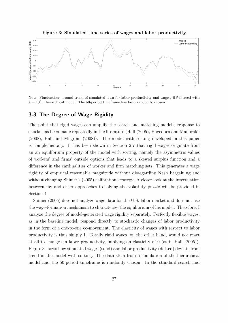
Figure 3: Simulated time series of wages and labor productivity
5 10 15 20 25 30 35 40 45 50
−0.04
−0.03
−0.02
−0.01
0
0.01
0.02
0.03
0.04
Periods
Pe
rce
nta
ge
de
via
tio
n f
rom
ste
ad
y s
tate
Wages
Labor Productivity
Note: Fluctuations around trend of simulated data for labor productivity and wages, HP-filtered withλ = 105. Hierarchical model. The 50-period timeframe has been randomly chosen.
3.3 The Degree of Wage Rigidity
The point that rigid wages can amplify the search and matching model’s response to
shocks has been made repeatedly in the literature (Hall (2005), Hagedorn and Manovskii
(2008), Hall and Milgrom (2008)). The model with sorting developed in this paper
is complementary. It has been shown in Section 2.7 that rigid wages originate from
an an equilibrium property of the model with sorting, namely the asymmetric values
of workers’ and firms’ outside options that leads to a skewed surplus function and a
difference in the cardinalities of worker and firm matching sets. This generates a wage
rigidity of empirical reasonable magnitude without disregarding Nash bargaining and
without changing Shimer’s (2005) calibration strategy. A closer look at the interrelation
between my and other approaches to solving the volatility puzzle will be provided in
Section 4.
Shimer (2005) does not analyze wage data for the U.S. labor market and does not use
the wage-formation mechanism to characterize the equilibrium of his model. Therefore, I
analyze the degree of model-generated wage rigidity separately. Perfectly flexible wages,
as in the baseline model, respond directly to stochastic changes of labor productivity
in the form of a one-to-one co-movement. The elasticity of wages with respect to labor
productivity is thus simply 1. Totally rigid wages, on the other hand, would not react
at all to changes in labor productivity, implying an elasticity of 0 (as in Hall (2005)).
Figure 3 shows how simulated wages (solid) and labor productivity (dotted) deviate from
trend in the model with sorting. The data stem from a simulation of the hierarchical
model and the 50-period timeframe is randomly chosen. In the standard search and
27

matching model, these two time series would simply be congruent. Wages are fully
flexible and instantaneously adjust whenever stochastic labor productivity changes. In
the depicted model with sorting, however, wages turn out to be less volatile and do not
fully adjust, as can be seen in Figure 3. The amplitude of labor productivity deviations
(dotted) is considerably larger. Hence the elasticity of wages with respect to labor
productivity must be somewhat smaller than 1. This is exactly the result one would
expect. In the baseline model, wages are too responsive. After a favorable shock, workers
soak up most of the extra productivity via wages since they immediately adjust what
leads to insufficient responsiveness of other model variables, particularly vacancies, due
to a lack of incentives for the firm. In the model with sorting, however, the one-to-one
link between wages and labor productivity is dampened. The arising wage rigidity, which
is visible in Figure 3, limits the extent to which wages adjust in response to the shock.
This increases firm’s incentives to create new jobs and leads to amplification.
To check whether the model-generated rigidity is of a reasonable magnitude, I refer
to the empirical literature on this issue. I rely on Haefke et al. (2013), who focus pri-
marily on the different degrees of wage rigidity for newly hired workers as compared to
established employment relationships. I can compare the reported wage-elasticity with
respect to labor productivity for new hires to my results. Haefke et al. (2013) note that
this value “is an appropriate and informative calibration target for search and matching
models.”27 The authors find an elasticity of wages with respect to labor productivity
of 0.8 with a relatively large standard error of 0.4. Using data from simulations of the
model with sorting, this elasticity can simply be computed as the coefficient η1 of a
simple linear regression of wages on labor productivity in logs and first differences:
∆ logWt(s, c) = η0 + η1∆ log Yt + εt (26)
Running this simple regression yields a wage elasticity of η1 = 0.751 for the hierarchical
model and η1 = 0.871 in the circular case. These elasticities lie well within the em-
pirically supported range. Hagedorn and Manovskii (2008) also compute an elasticity
from U.S. wage and productivity data and report a coefficient of 0.449, which also lies
27 Haefke et al. (2013), p. 898. Since the baseline search and matching model with Nash bargaining isessentially a model of new hires, the elasticity of wages with respect to labor productivity for thisgroup is a reasonable metric to assess the plausibility of the theoretical model and the simulationresults. Note that wages do not play any allocational role in a random search model. The Nashbargaining solution simply determines how the surplus is shared in every time-period given the stateof the model in the same period. Thus, the length of an employment spell does not influence wagesand there is no meaningful distinction between new hires and existing employment relationships.
28

within the supported range, albeit at the lower end. The elasticity/derivative implied
by the alternating-offer bargaining game proposed by Hall and Milgrom (2008) is about
0.7, again in line with both the empirical evidence and the endogenous wage rigidity
generated by the model with sorting. It is reassuring that the rigidity lies close to these
benchmarks.
Recall that the endogenous wage rigidity is, as described above, not the only modi-
fication of the model with sorting. Given the strong amplification effect, the degree of
wage rigidity I find appears to be small at first sight. However, the value is well in line
with empirical evidence on wage rigidities, a more extreme kind of rigidity would not be
justified. It is thus instructive to decompose the effect of sorting in the dynamic model
according to the two sources of amplification: The endogenous wage rigidity and the
additional margin of adjustment in job-creation.
3.4 Rigid Wages vs. Job-Creation
Besides amplification due to rigid wages, sorting unfolds a second effect that leads to am-
plification via forward-looking vacancy posting decisions. Recall the firms’ job creation
condition, equation (15), with Mt′/Vt′ plugged in for qvt′ :
κVt′
Mt′= β(1− α)
∫Ms
t′ (c)
gut′(s)
Ut′St′(s, c) ds. (27)
After a positive productivity shock hits the economy, the inversely U-shaped surplus
function shifts upwards. Firms choose wider matching sets because the surplus from an
increased number of potential matches is larger than zero. This leads to a higher expected
value of future surpluses on the side of the firm and, consequentially, amplification.
The difference to the standard model is precisely this effect of the fluctuating matching
sets. Not only the surplus increases in response to the shock. The margins of the
firms’ matching sets get wider too. This implies that for a productivity shock of equal
magnitude, the RHS of (27) in the model with sorting experiences a larger increase
than the corresponding equation in the standard model would lead to. This additional
margin of adjustment via the matching set has to be offset by a larger number of vacancy
postings, V , which is the firm’s control variable. Thus, in this model wages do not need
to be extremely rigid (as in Hall (2005)) to generate sufficient volatility. A higher number
of additional vacancy postings is the optimal response to a positive shock as compared
to the standard model. This generates more amplification than the wage-rigidity alone.
29
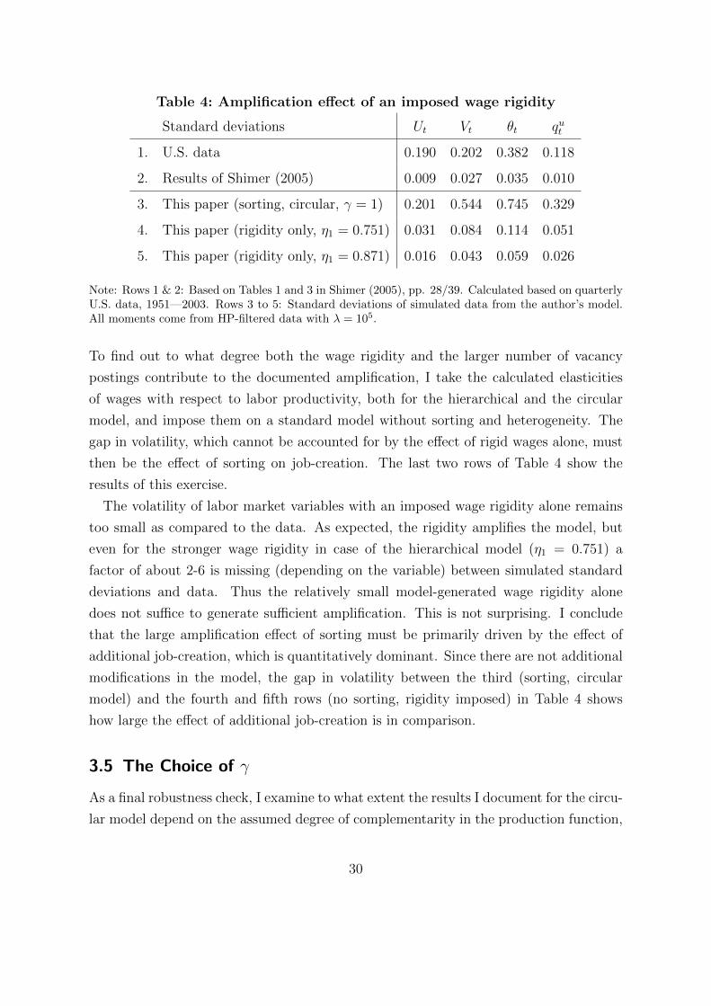
Table 4: Amplification effect of an imposed wage rigidity
Standard deviations Ut Vt θt qut
1. U.S. data 0.190 0.202 0.382 0.118
2. Results of Shimer (2005) 0.009 0.027 0.035 0.010
3. This paper (sorting, circular, γ = 1) 0.201 0.544 0.745 0.329
4. This paper (rigidity only, η1 = 0.751) 0.031 0.084 0.114 0.051
5. This paper (rigidity only, η1 = 0.871) 0.016 0.043 0.059 0.026
Note: Rows 1 & 2: Based on Tables 1 and 3 in Shimer (2005), pp. 28/39. Calculated based on quarterlyU.S. data, 1951—2003. Rows 3 to 5: Standard deviations of simulated data from the author’s model.All moments come from HP-filtered data with λ = 105.
To find out to what degree both the wage rigidity and the larger number of vacancy
postings contribute to the documented amplification, I take the calculated elasticities
of wages with respect to labor productivity, both for the hierarchical and the circular
model, and impose them on a standard model without sorting and heterogeneity. The
gap in volatility, which cannot be accounted for by the effect of rigid wages alone, must
then be the effect of sorting on job-creation. The last two rows of Table 4 show the
results of this exercise.
The volatility of labor market variables with an imposed wage rigidity alone remains
too small as compared to the data. As expected, the rigidity amplifies the model, but
even for the stronger wage rigidity in case of the hierarchical model (η1 = 0.751) a
factor of about 2-6 is missing (depending on the variable) between simulated standard
deviations and data. Thus the relatively small model-generated wage rigidity alone
does not suffice to generate sufficient amplification. This is not surprising. I conclude
that the large amplification effect of sorting must be primarily driven by the effect of
additional job-creation, which is quantitatively dominant. Since there are not additional
modifications in the model, the gap in volatility between the third (sorting, circular
model) and the fourth and fifth rows (no sorting, rigidity imposed) in Table 4 shows
how large the effect of additional job-creation is in comparison.
3.5 The Choice of γ
As a final robustness check, I examine to what extent the results I document for the circu-
lar model depend on the assumed degree of complementarity in the production function,
30
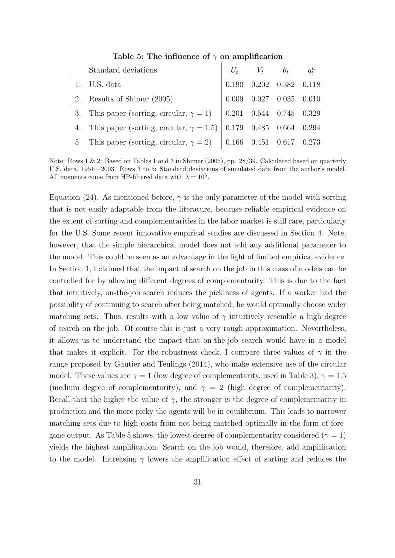
Table 5: The influence of γ on amplification
Standard deviations Ut Vt θt qut
1. U.S. data 0.190 0.202 0.382 0.118
2. Results of Shimer (2005) 0.009 0.027 0.035 0.010
3. This paper (sorting, circular, γ = 1) 0.201 0.544 0.745 0.329
4. This paper (sorting, circular, γ = 1.5) 0.179 0.485 0.664 0.294
5. This paper (sorting, circular, γ = 2) 0.166 0.451 0.617 0.273
Note: Rows 1 & 2: Based on Tables 1 and 3 in Shimer (2005), pp. 28/39. Calculated based on quarterlyU.S. data, 1951—2003. Rows 3 to 5: Standard deviations of simulated data from the author’s model.All moments come from HP-filtered data with λ = 105.
Equation (24). As mentioned before, γ is the only parameter of the model with sorting
that is not easily adaptable from the literature, because reliable empirical evidence on
the extent of sorting and complementarities in the labor market is still rare, particularly
for the U.S. Some recent innovative empirical studies are discussed in Section 4. Note,
however, that the simple hierarchical model does not add any additional parameter to
the model. This could be seen as an advantage in the light of limited empirical evidence.
In Section 1, I claimed that the impact of search on the job in this class of models can be
controlled for by allowing different degrees of complementarity. This is due to the fact
that intuitively, on-the-job search reduces the pickiness of agents. If a worker had the
possibility of continuing to search after being matched, he would optimally choose wider
matching sets. Thus, results with a low value of γ intuitively resemble a high degree
of search on the job. Of course this is just a very rough approximation. Nevertheless,
it allows us to understand the impact that on-the-job search would have in a model
that makes it explicit. For the robustness check, I compare three values of γ in the
range proposed by Gautier and Teulings (2014), who make extensive use of the circular
model. These values are γ = 1 (low degree of complementarity, used in Table 3), γ = 1.5
(medium degree of complementarity), and γ = 2 (high degree of complementarity).
Recall that the higher the value of γ, the stronger is the degree of complementarity in
production and the more picky the agents will be in equilibrium. This leads to narrower
matching sets due to high costs from not being matched optimally in the form of fore-
gone output. As Table 5 shows, the lowest degree of complementarity considered (γ = 1)
yields the highest amplification. Search on the job would, therefore, add amplification
to the model. Increasing γ lowers the amplification effect of sorting and reduces the
31

excess volatility of vacancies. This is intuitive: Very picky agents in equilibrium and a
corresponding high degree of complementarity imply that for the same magnitude of the
productivity shock the matching sets will adjust less. In other words, a higher additional
value of surplus is necessary to increase the cardinality of the matching sets by the same
amount. This pattern emerges simply as an equilibrium property of the surplus function.
The surface of positive surpluses is much steeper in case of high complementarity due
to the large gains from being optimally matched. Hence, matching sets fluctuate less in
response to shocks and the additional margin in the job-creation condition is dampened,
what leads to less amplification with large complementarity. The discrepancy between
the volatility of unemployment and vacancies remains, however. It is not possible to
perfectly adjust the search and matching model with sorting to the data by calibrating
γ alone. Instead, empirical evidence for the importance of complementarity and sorting
in the U.S. labor market is necessary to make an informed choice.
4 Discussion in Relation to the Literature
This paper constructs an equilibrium search and matching model with two-sided het-
erogeneity and sorting. Gautier et al. (2006) provide an insightful overview of the devel-
opment of this class of labor search models. The relationship to the previous literature
is best understood from two reference points. The first reference point is the assign-
ment game among heterogeneous agents in a frictionless market following Becker (1973).
Becker characterizes the equilibrium of a marriage market, that is, a market with non-
transferable utility. In this frictionless, neoclassical model, all types are only willing
to match with their one optimal counterparts to form matches which jointly maximize
payoffs. Thus, matching sets consist of only a single element. Shimer and Smith (2000)
take this model out of its Walrasian equilibrium by adding frictions and costly search.
Additionally, they consider transferable utility, thereby building a bridge to labor market
applications of the theory. In their paper, technical conditions for positive assortative
matching in equilibrium are derived and existence is proven: in a nutshell, types need to
be complements in production. Thus, models featuring positive sorting rely on a super-
modular production function which is increasing in its two arguments, the worker’s skill
and the firm’s productivity, and twice continuously differentiable.The second reference
point is the baseline search and matching model of the labor market as outlined in the
textbook by Pissarides (2000) and used in—among many other papers—Shimer (2005).
The DMP model has been very successful due to its ability to explain equilibrium un-
32

employment and a number of important stylized facts of labor market data (e.g. the
Beveridge curve). Due to the fact that it abstracts from heterogeneity and thus consid-
ers only one representative type of workers and firms, the matching sets of those types
embrace the whole type space.28 In other words, every agent is willing to match with
every other agent, but frictions limit the number of encounters in the labor market and,
therefore, unemployment exists. Wages are totally flexible in this model. In a dynamic
framework with aggregate uncertainty, they adjust instantaneously and follow labor pro-
ductivity one-to-one. This point is central to the discussion started by Shimer (2005)
and Hall (2005). Shimer (2005) points out that even though the standard search and
matching framework appealingly predicts the long-run equilibrium of the labor market,
the volatility of data from stochastic simulations of the baseline model is too small by
a factor of up to 20 compared to empirical second moments of U.S. labor market data.
This obstacle has become known as the Shimer Puzzle. Departure from totally flexible
wages, that is, incorporating rigid wages into the baseline model, has been used to solve
this problem since rigid wages increase firms’ incentives to create jobs in a cyclical up-
swing, that is, in response to a positive productivity shock.29 Due to the rigidity, wages
no longer follow labor productivity one-to-one. Thus, wages become less volatile and
the dynamics of the model are amplified since more vacancies will be posted until the
firms’ free entry condition is satisfied. However, the assumptions used in the literature
to justify rigid wages are highly debated. Hall (2005) shows that the volatility puzzle
vanishes once wages are made fully inflexible. This, however, implies a counterfactual
wage volatility of zero. Hagedorn and Manovskii (2008) show that the dynamics can be
amplified by increasing the value of the workers’ outside option of non-market activity. A
higher calibrated value of the respective model parameter leads to lower wage outcomes
in the Nash bargaining game, however, with rather unrealistic consequences.30
I construct a model in between the two reference points: in a labor market with search
frictions and assortativeness through complementarity, suboptimal matches between het-
erogeneous jobs and workers arise in equilibrium and persist through time. This setup
generates sufficient volatility in a search and matching model without the additional
28 Which is simply a point.29 The baseline model is calibrated to ensure that vacancy posting is socially efficient according to the
Hosios (1990) condition. This leads to a too-high share of the additional surplus for the worker anddiminishes firms’ incentives to post additional jobs given free entry, which leads to the well-knownproblem that labor market variables react insufficiently to a shock.
30 Hornstein et al. (2005) and Costain and Reiter (2008) conclude that the calibration strategy pro-posed by Hagedorn and Manovskii (2008) is implausible because a 15% increase in the value ofnon-market activity implies that the unemployment rate doubles.
33

assumptions that earlier approaches made.31
Frictions rationalize the formation of matches beyond the optimal allocation of work-
ers to jobs because heterogeneity and match-specific output give rise to the possibility
that the option value of continued search for the optimal partner is lower than the
option value of starting production immediately. The key object of this optimal stop-
ping problem is the production function and the degree of complementarity between its
inputs, worker skills and firm productivity. It governs the acceptable degree of subop-
timality, that is, the acceptable divergence from the first-best allocation. The higher
the degree of complementarity between the inputs of the production function is, the
higher is the penalty from a suboptimal match in form of foregone output leading to
narrower matching sets and a higher aggregate welfare-loss relative to the optimal allo-
cation. The production function’s degree of complementarity is thus a parameter of high
empirical interest, also because the degree of sorting contains important implications for
policies which are concerned with the optimal allocation of scarce resources in the labor
market. A large literature attempts to identify the sign and strength of sorting using
matched employer-employee data and reduced form empirical models with worker and
firm fixed effects representing unobservable worker and firm characteristics. (see Abowd
et al. (1999) and follow-up papers). While adding fixed effects considerably improves
those models’ explanatory power regarding wage dispersion, many authors inferred that
sorting does not systematically affect wage formation because the correlation between
the two fixed effects is typically statistically indistinguishable from zero. If positive sort-
ing played a significant role in explaining wage formation, one would expect to find a
strong positive correlation between the two fixed effects.
An empirical and intuitive explanation for this small correlation of worker and firm
fixed effects is the so-called limited mobility bias (Andrews et al. (2008), Andrews et al.
(2012)). It implies that estimated correlations are biased downwards. A conclusion
regarding the importance of sorting for wage determination would thus be misleading.
The fewer observations of movers between firms in matched employer-employee data
there are, the larger the bias and the smaller is the estimated correlation.32
31 The impact of worker heterogeneity on the dynamics of a search and matching model is also inthe focus of an interesting article by Pries (2008). He analyzes how worker heterogeneity canimpact the dynamics of a search and matching model, however, without analyzing wage formationin particular. He introduces heterogeneity, two types of workers and homogenous firms, in a muchsimpler way than this paper. Pries (2008) finds some amplification, which he ascribes to a changingcomposition of the pool of unemployed workers over the business cycle. However, this modificationdoes not to sufficiently amplify the model.
32 Using German data, Andrews et al. (2012) find positive correlations between worker and firm fixedeffects for establishments with a large number of movers and thus conclude that the true correlation
34
Eeckhout and Kircher (2011) present a theoretical argument why one cannot conclude
that sorting is irrelevant for match formation and wage determination in the labor mar-
ket based on inference from reduced form empirical models. The key argument is that,
in theory, assortative matching leads to type-specific wages which, for a given worker,
do not monotonically increase in the type of the firm. The fixed effects methodology
used in studies that build on Abowd et al. (1999) cannot account for such non-linear
relations between the unobserved time-invariant determinants of wages as it necessitates
additive separability. A theoretical model with sorting, however, implies an inverted
U-shape pattern of a given worker’s wages in the firm type. This is also a feature of the
model presented in this paper. Beyond the extremum of this non-monotonous function,
which represents the first best allocation of this worker and his highest achievable wage,
remuneration is lower because the worker has to compensate the firm for hiring him
and not waiting to match with a more suitable candidate. Due to search frictions, the
probability of matching with the optimal type on a continuous type space is zero for
both workers and firms. They have to decide about the acceptable degree of mismatch
by optimally choosing the width of their matching sets. The condition for a type to
be an element of the matching set is a high enough surplus to compensate both parties
for the foregone option value of continued search. While it is impossible to identify the
sign of sorting in the simple two-period model used by Eeckhout and Kircher (2011)
with wage data alone, Hagedorn et al. (2012) show that the production function—and
thus the sign and strength of sorting—is non-parametrically identifiable using standard
matched employer-employee data and a fully-dynamic search model with discounting.
In a different paper that focuses on workers’ search intensity as driving force of sorting,
Bagger and Lentz (2014) also solve this identification problem and document significant
positive sorting for the Danish labor market using state-of-the-art structural economet-
ric techniques. Due to a renewed and broad interest in the empirical identification of
labor market sorting, more evidence for different countries can be expected in the near
future. From this papers perspective, these new insights are critically important. I show
that sorting has the potential to increase our understanding of labor market dynamics.
Since positive sorting is the central assumption of the model, the key parameter of the
production function, which governs sorting via the degree of complementarity, has to be
calibrated in an informed way using sound empirical evidence, see Section 3.5.
should be positive for Germany. Mendes et al. (2010) document comparable evidence in supportof positive sorting. Using very detailed Portuguese data, the authors construct a measure of firm-specific productivity and thus do not have to rely on firm fixed effects. They find strong evidencefor PAM in Portugal.
35

Rigidities of prices and wages play a key role in modern macroeconomics. Blanchard
and Galı (2010) show how nominal rigidities influence aggregate fluctuations in a DSGE
model with a search and matching labor market component. The key insight is that
the central bank faces a trade-off between inflation and unemployment fluctuations if
and only if inefficient unemployment fluctuations arise in the presence of productivity
shocks. This can only be the case, however, if the labor market block of the DSGE
model generates a sufficient degree of amplification in response to shocks. Otherwise
unemployment would simply not be responsive on a meaningful scale, contrary to the
data. Thus, the Shimer puzzle plays a key role also in enabling larger macroeconomic
models to generate dynamics which are consistent with the data and, thus, allow for
model-based policy advice in the presence of macroeconomic fluctuations. Blanchard and
Galı (2010) also survey a number of earlier papers that explored the implications of real
and nominal rigidities in different variants of real business cycle (RBC) or New-Keynesian
macro (NKM) models and also link them to the Shimer puzzle literature. The models
developed by Merz (1995), Andolfatto (1996), Christoffel and Linzert (2005), Krause
and Lubik (2007), Faia (2008), and Gertler and Trigari (2009), among many others,
are all examples of complex DSGE models, studied through calibration and simulation,
that integrate variants of price and wage staggering to create persistence and sufficient
amplification for the analysis of different kinds of shocks. Gertler and Trigari (2009),
for example, adapt the well-known Calvo (1983) pricing structure for wage formation in
the labor market. Rigid wages are generated by only allowing a calibrated fraction of
matches to renegotiate wages in every period. This complex and empirically reasonable
modification brings the model’s dynamics considerably closer to the data. The key
contribution of this paper, in the light of the literature surveyed by Blanchard and Galı
(2010), is that the search and matching model with two-sided heterogeneity and sorting
is able to generate rigid wages as well as large and inefficient unemployment fluctuations,
in line with the data, without additional model extensions. Intuitively, the channels of
transmission are similar to those explored in the literature. This shows that sufficient
amplification in the presence of shocks and the simple Nash bargaining solution are not
necessarily mutually exclusive.
The model developed in this paper is closely related to the standard DMP models that
have been extensively analyzed in the literature mentioned above. It can even be shown
that it nests the textbook model. Once the continuous type-space is collapsed into a
single point, that is, in case of one representative worker and firm, the equations simplify
to their textbook versions. Therefore, the mechanism of transmission in the presence
36

of productivity shocks are transparent and the results are directly applicable to larger
macroeconomic models. Thus, incorporating a frictional labor market with sorting into
a large macroeconomic model with heterogeneous agents is a fascinating topic for future
research. One should, however, keep in mind the well-known limitations of the standard
search and matching model. First, the model uses a linear search technology in the form
of an aggregate matching function with constant returns to scale. While this approach
has not been rejected by the data in numerous empirical studies (for a summary, see
Petrongolo and Pissarides (2001)), it is by no means undisputed.33 Second, the assump-
tion that only unemployed individuals search might be less convincing in a model with
heterogeneity. The literature contains some empirical evidence on job-to-job flows (for
the United States, see, e.g., Fallick and Fleischman (2004) and Nagypal (2005)). I em-
phasized, however, that search on-the-job would not alter the main results of this paper
qualitatively since it would simply imply wider matching sets in equilibrium, similar to
a smaller value of γ in my model. Lise et al. (2013) and Lise and Robin (2014) indeed
show that apply a sequential bargaining framework in the spirit of Postel-Vinay and
Robin (2002) to allow for on-the-job search and poaching also lead to empirically sound
dynamics. However, these richer models cannot be applied directly to the literature on
wage rigidity and the Shimer Puzzle, which is the focus and central contribution of this
paper.
5 Conclusions
Explaining the market imperfections that one can observe in the data in form of sluggish
and imperfect price adjustments is a key challenge of modern macroeconomics. Only
taking these rigidities into account enables macroeconomic models to generate dynamics
which are consistent with empirical facts. Thus, many papers rely on complex model
extensions to generate rigid prices and wages to match the data. Often, the labor
market is in the center of attention because rigid wages can be the source of inefficient
unemployment fluctuations over the business cycle, what is by many considered to be
a key labor market policy concern. Search and matching models are the workhorse
33 Kohlbrecher et al. (2014) show in a recent working paper how the characteristic co-movement ofmatches and unemployment/vacancies can also arise in a model without a matching function dueto idiosyncratic labor productivity and free entry. Thus, matching function estimations might beseriously biased. Additionally, Borowczyk-Martins et al. (2013) emphasize that empirical modelsthat estimate the elasticities of a standard matching function can be severely biased due to endo-geneity. They propose an empirical strategy that eliminates this bias by using lagged values of thekey variables as instruments.
37

environment in this kind of application. However, the most widely applied version
features fully flexible wages and cannot create rigidities and sufficient amplification by
itself.
This paper shows how two-sided ex-ante heterogeneity and a production function with
complementarity, i.e., positive assortative matching, can help to overcome this shortcom-
ing and improve the canonical search and matching model’s ability to match empirical
moments of labor market data. The model endogenously generates a wage rigidity and
does not rely on any additional assumptions besides heterogeneity and sorting. Addition-
ally, the recent advances in capturing the extent of assortative matching in labor markets
empirically (Andrews et al. (2008), Lopes de Melo (2009), Eeckhout and Kircher (2011),
Hagedorn et al. (2012), Bartolucci and Devicienti (2013), Bagger and Lentz (2014)) will
increasingly enable the researcher to plausibly measure and calibrate the degree of sort-
ing and complementarity. Some evidence in favor of positive sorting is already presented
in some of those studies. The approach to generate rigid wages and sufficient amplifi-
cation in a search and matching model that is presented in this paper is thus a both
microfounded and empirically supported complement to existing approaches to better
align search and matching models with the data.
The endogenous wage rigidity I find is of empirically reasonable magnitude. Together
with the effect of sorting on firms’ vacancy posting decisions, it enables the model to
overcome Shimer’s volatility puzzle. Both effects provide additional incentives for firms
to create jobs in response to a favorable productivity shock. This mechanism significantly
amplifies the simulated standard deviations of unemployment, vacancies, labor market
tightness, and the job-finding rate compared to the baseline model of Shimer (2005).
Aside from the added heterogeneity, the model’s elements are standard in the literature
and it collapses to the Pissarides (2000) textbook search and matching model for the case
of homogenous workers and firms. Thus, I can rely on the empirical results of Shimer
(2005) to calibrate the model and comparability of my results is ensured. The improved
dynamic properties are solely a result of explicitly accounting for assortative matching.
38

References
Abowd et al. 1999 Abowd, John M. ; Kramarz, Francis ; Margolis, David N.:
High Wage Workers and High Wage Firms. In: Econometrica 67 (1999), No. 2, pp. 251
– 333
Adjemian et al. 2014 Adjemian, Stephane ; Bastani, Houtan ; Karame,
Frederic ; Juillard, Michel ; Maih, Junior ; Mihoubi, Ferhat ; Perendia, George ;
Pfeifer, Johannes ; Ratto, Marco ; Villemot, Sebastien: Dynare: Reference
Manual Version 4 / CEPREMAP. 2014 (1). – Dynare Working Papers
Andolfatto 1996 Andolfatto, David: Business Cycles and Labor-Market Search.
In: American Economic Review 86 (1996), No. 1, pp. 112 – 132
Andrews et al. 2008 Andrews, M. J. ; Gill, L. ; Schank, T. ; Upward, R.:
High Wage Workers and Low Wage Firms: Negative Assortative Matching or Limited
Mobility Bias? In: Journal of the Royal Statistical Society. Series A (Statistics in
Society) 171 (2008), No. 3, pp. pp. 673–697
Andrews et al. 2012 Andrews, M.J. ; Gill, L. ; Schank, T. ; Upward, R.: High
wage workers match with high wage firms: Clear evidence of the effects of limited
mobility bias. In: Economics Letters 117 (2012), No. 3, pp. 824 – 827
Bagger and Lentz 2014 Bagger, Jesper ; Lentz, Rasmus: An Empirical Model
of Wage Dispersion with Sorting / National Bureau of Economic Research. April 2014
(20031). – Working Paper
Bartolucci and Devicienti 2013 Bartolucci, Cristian ; Devicienti, Francesco:
Better Workers Move to Better Firms: A Simple Test to Identify Sorting / Society
for Economic Dynamics. 2013 (249). – 2013 Meeting Papers
Becker 1973 Becker, Gary S.: A Theory of Marriage: Part I. In: Journal of
Political Economy 81 (1973), No. 4, pp. 813 – 846
Blanchard and Galı 2010 Blanchard, Olivier ; Galı, Jordi: Labor Markets
and Monetary Policy: A New Keynesian Model with Unemployment. In: American
Economic Journal: Macroeconomics 2 (2010), No. 2, pp. 1 – 30
39

Borowczyk-Martins et al. 2013 Borowczyk-Martins, Daniel ; Jolivet, Gre-
gory ; Postel-Vinay, Fabien: Accounting for endogeneity in matching function
estimation. In: Review of Economic Dynamics 16 (2013), No. 3, pp. 440 – 451
Calvo 1983 Calvo, Guillermo A.: Staggered Prices in a Utility-Maximizing Frame-
work. In: Journal of Monetary Economics 12 (1983), No. 3, pp. 383 – 398
Christoffel and Linzert 2005 Christoffel, Kai ; Linzert, Tobias: The Role
of Real Wage Rigitity and Labor Market Frictions for Unemployment and Inflation
Dynamics. 2005. – European Central Bank Working Paper 556
Costain and Reiter 2008 Costain, James S. ; Reiter, Michael: Business cycles,
unemployment insurance, and the calibration of matching models. In: Journal of
Economic Dynamics and Control 32 (2008), No. 4, pp. 1120 – 1155
Eeckhout and Kircher 2011 Eeckhout, Jan ; Kircher, Philipp: Identifying
Sorting–In Theory. In: Review of Economic Studies 78 (2011), No. 3, pp. 872 – 906
Faia 2008 Faia, Ester: Optimal Monetary Policy Rules with Labor Market Frictions.
In: Journal of Economic Dynamics and Control 32 (2008), No. 5, pp. 1600 – 1621
Fallick and Fleischman 2004 Fallick, Bruce C. ; Fleischman, Charles A.:
Employer-to-Employer Flows in the U.S. Labor Market: The Complete Picture of
Gross Worker Flows. 2004. – Federal Reserve Board Finance and Economics Discus-
sion Paper 2004-34
Gautier and Teulings 2006 Gautier, Pieter A. ; Teulings, Coen N.: How large
are search frictions? In: Journal of the European Economic Association 4 (2006),
No. 6, pp. 1193–1225
Gautier and Teulings 2014 Gautier, Pieter A. ; Teulings, Coen N.: Sorting
and the output loss due to search frictions. 2014
Gautier et al. 2006 Gautier, Pieter A. ; Teulings, Coen N. ; Van Vuuren, Aico:
Structural Models of Wage and Employment Dynamics: Contributions to Economics
Analysis. Chap. Labor Market Search with Two-Sided Heterogeneity: Hierarchical
versus Circular Models, pp. 117–132, Pergamon Press, 2006
Gautier et al. 2010 Gautier, Pieter A. ; Teulings, Coen N. ; Van Vuuren,
Aico: On-the-Job Search, Mismatch and Efficiency. In: Review of Economic Studies
77 (2010), No. 1, pp. 245 – 272
40

Gertler and Trigari 2009 Gertler, Mark ; Trigari, Antonella: Unemployment
Fluctuations with Staggered Nash Wage Bargaining. In: Journal of Political Economy
117 (2009), No. 1, pp. 38 – 86
Haefke et al. 2013 Haefke, Christian ; Sonntag, Marcus ; Rens, Thijs van: Wage
rigidity and job creation. In: Journal of Monetary Economics 60 (2013), No. 8, pp. 887
– 899
Hagedorn et al. 2012 Hagedorn, Marcus ; Law, Tzuo H. ; Manovskii, Iourii:
Identifying Equilibrium Models of Labor Market Sorting / National Bureau of Eco-
nomic Research. December 2012 (18661). – Working Paper
Hagedorn and Manovskii 2008 Hagedorn, Marcus ; Manovskii, Iourii: The
Cyclical Behavior of Equilibrium Unemployment and Vacancies Revisited. In: The
American Economic Review 98 (2008), No. 4, pp. 1692 – 1706
Hall 2005 Hall, Robert E.: Employment Fluctuations with Equilibrium Wage
Stickiness. In: The American Economic Review 95 (2005), No. 1, pp. 50 – 65
Hall and Milgrom 2008 Hall, Robert E. ; Milgrom, Paul R.: The Limited
Influence of Unemployment on the Wage Bargain. In: American Economic Review 98
(2008), No. 4, pp. 1653 – 1674
Hornstein et al. 2005 Hornstein, Andreas ; Krusell, Per ; Violante, Giovanni:
Unemployment and Vacancy Fluctuations in the Matching Model: Inspectiong the
Mechanism. In: Federal Reserve of Richmond Economic Quarterly 91 (2005), No. 3,
pp. 19 – 51
Hosios 1990 Hosios, Arthur J.: On the Efficiency of Matching and Related Models
of Search and Unemployment. In: The Review of Economic Studies 57 (1990), No. 2,
pp. 279 – 298
Kohlbrecher et al. 2014 Kohlbrecher, Britta ; Merkl, Christian ; Nordmeier,
Daniela: Revisiting the Matching Function / Kiel Institute for the World Economy.
February 2014 (1909). – Kiel Working Paper
Krause and Lubik 2007 Krause, Michael U. ; Lubik, Thomas A.: The
(Ir)Relevance of Real Wage Rigidity in the New Keynesian Model with Search Fric-
tions. In: Journal of Monetary Economics 54 (2007), No. 3, pp. 706 – 727
41

Lise et al. 2013 Lise, Jeremy ; Meghir, Costas ; Robin, Jean-Marc: Mismatch,
Sorting and Wage Dynamics / National Bureau of Economic Research. January 2013
(18719). – Working Paper
Lise and Robin 2014 Lise, Jeremy ; Robin, Jean-Marc: The Macro-dynamics of
Sorting between Workers and Firms. December 2014
Marimon and Zilibotti 1999 Marimon, Ramon ; Zilibotti, Fabrizio: Unem-
ployment vs. Mismatch of Talents: Reconsidering Unemployment Benefits. In: The
Economic Journal 109 (1999), No. 455, pp. pp. 266–291
Lopes de Melo 2009 Melo, Rafael Lopes de: Sorting in the Labor Market: Theory
and Measurement / Universtiy of Chicago. December 2009. – Discussion paper
Mendes et al. 2010 Mendes, Rute ; Berg, Gerard J. van den ; Lindeboom,
Maarten: An empirical assessment of assortative matching in the labor market. In:
Labour Economics 17 (2010), No. 6, pp. 919 – 929. – ISSN 0927-5371
Merz 1995 Merz, Monika: Search in the Labor Market and the Real Business Cycle.
In: Journal of Monetary Economics 36 (1995), No. 2, pp. 269 – 300
Mortensen and Pissarides 1994 Mortensen, Dale T. ; Pissarides, Christo-
pher A.: Job Creation and Job Destruction in the Theory of Unemployment. In:
Review of Economic Studies 61 (1994), pp. 397 – 415
Nagypal 2005 Nagypal, Eva: On the extent of job-to-job transitions. 2005. –
Working Paper
Petrongolo and Pissarides 2001 Petrongolo, Barbara ; Pissarides, Christo-
pher A.: Looking into the Black Box: A Survey of the Matching Function. In: Journal
of Economic Literature 39 (2001), June, No. 2, pp. 390 – 431
Pissarides 2000 Pissarides, Christopher A.: Equilibrium Unemployment Theory.
2nd Edition. The MIT Press, 2000
Pissarides 2009 Pissarides, Christopher A.: The Unemployment Volatility Puzzle:
Is Wage Stickiness the Answer? In: Econometrica 77 (2009), No. 5, pp. 1339 – 1369
Postel-Vinay and Robin 2002 Postel-Vinay, Fabien ; Robin, Jean-Marc: Equi-
librium Wage Dispersion with Worker and Employer Heterogeneity. In: Econometrica
70 (2002), No. 6, pp. 2295–2350
42

Pries 2008 Pries, Michael J.: Worker heterogeneity and labor market volatility in
matching models. In: Review of Economic Dynamics 11 (2008), No. 3, pp. 664 – 678
Robin 2011 Robin, Jean-Marc: On the Dynamics of Unemployment and Wage
Distributions. In: Econometrica 79 (2011), No. 5, pp. 1327–1355
Rubinstein 1982 Rubinstein, Ariel: Perfect Equilibrium in a Bargaining Model.
In: Econometrica 50 (1982), No. 1, pp. pp. 97–109
Shimer 2005 Shimer, Robert: The Cyclical Behavior of Equilibrium Unemployment
and Vacancies. In: The American Economic Review 95 (2005), No. 1, pp. 25 – 49
Shimer and Smith 2000 Shimer, Robert ; Smith, Lones: Assortative Matching
and Search. In: Econometrica 68 (2000), March, No. 2, pp. 343 – 369
Teulings 2005 Teulings, Coen N.: Comparative Advantage, Relative Wages, and
the Accumulation of Human Capital. In: Journal of Political Economy 113 (2005),
No. 2, pp. 425–461
Teulings and Gautier 2004 Teulings, Coen N. ; Gautier, Pieter A.: The Right
Man for the Job. In: The Review of Economic Studies 71 (2004), No. 2, pp. 553–580
Topkis 1998 Topkis, Donald M.: Supermodularity and Complementarity. Princeton
University Press, 1998
43