volume technical university of cluj-napoca north

Carp

ath

ian

Jo

urn

al o

f E

lectr

ical E

ng

ineeri

ng

V

olu

me 11

, N

um

ber

1, 2

017

Volume 11, Number 1, 2017

Technical University of Cluj-Napoca

North University Centre of Baia Mare

Faculty of Engineering

Electrical, Electronic and Computer Engineering Department

Carpathian Journal of Electrical Engineering

UTPRESS PUBLISHER

ISSN 1843 - 7583

Carpathian Journal of Electrical Engineering

Volume 11, Number 1, 2017

ISSN 1843 – 7583 http://cee.ubm.ro/cjee.html

EDITOR-IN-CHIEF

Liviu NEAMȚ Technical University of Cluj-Napoca, Romania

ASSOCIATE EDITOR

Mircea HORGOŞ Technical University of Cluj-Napoca, Romania

EDITORIAL SECRETARY

Olivian CHIVER Technical University of Cluj-Napoca, Romania

SCIENTIFIC BOARD

Gene APPERSON Digilent Inc. SUA

Cristian BARZ Technical University of Cluj-Napoca, Romania

Florin BREABĂN Artois University, France

Vasilis CHATZIATHANASIOU Aristotle University of Thessaloniki, Greece

Clint COLE Washington State University, SUA

Iuliu DELESEGA Polytechnic University of Timişoara, Romania

Luis Adriano DOMINGUES Brazilian Electrical Energy Research Center, Brazil

Zoltan ERDEI Technical University of Cluj-Napoca, Romania

Patrick FAVIER Artois University, France

Ştefan MARINCA Analog Devices, Ireland

Andrei MARINESCU Research and Testing Institute ICMET, Romania

Oliviu MATEI Technical University of Cluj-Napoca, Romania

Tom O’DWYER Analog Devices, Ireland

Desire RASOLOMAMPIONONA Warsaw University of Technology, Poland

Alexandru SIMION Gheorghe Asachi Technical University of Iasi, Romania

Emil SIMION Technical University of Cluj-Napoca, Romania

Adam TIHMER University of Miskolc, Hungary

Theodoros D. TSIBOUKIS Aristotle University of Thessaloniki, Greece

Jan TURAN Technical University of Kosice, Slovakia

Jozsef VASARHELYI University of Miskolc, Hungary

Andrei VLADIMIRESCU University of California, Berkeley, USA

Carpathian Journal of Electrical Engineering Volume 11, Number 1, 2017

5

CONTENTS

Harun SUMBUL

FUZZY LOGIC-BASED AUTOMATIC DOOR CONTROL SYSTEM ..................................... 7

Ovidiu COSMA

IMAGE STEGANOGRAPHY TAILORED TO OBJECTS CONTOURS ................................ 17

Dumitru SPERMEZAN, Mircea I. BUZDUGAN, Horia BALAN

STRUCTURAL MONITORING OF WIND TURBINES USING SENSORS

CONNECTED VIA UTP CABLE.......................................................................................... 25

Ovidiu COSMA

A METHOD FOR DENOISING IMAGE CONTOURS ......................................................... 37

Horia BALAN, Mircea I. BUZDUGAN, Ionut IANCAU, Liviu NEAMT

TESTING SOLUTIONS OF THE PROTECTION SYSTEMS PROVIDED

WITH DELAY MAXIMUM CURRENT RELAYS .................................................................. 47

Lenin KANAGASABAI

DECLINE OF ACTIVE POWER LOSS BY IMPROVED MOTH-FLAME

OPTIMIZATION ALGORITHM ........................................................................................... 59

Bogdan IUGA, Radu-Adrian TIRNOVAN

BIOT-SAVART LAW APPLICATION IN WIRELESS POWER TRANSFER – DEPENDENCE

OF MAGNETIC FIELD TO ANGLE POSITION ................................................................. 73

INSTRUCTIONS FOR AUTHORS ....................................................................................... 79


6


7

FUZZY LOGIC-BASED AUTOMATIC DOOR CONTROL SYSTEM

Harun SUMBUL

Department of Biomedical Device Technologies, Yesilyurt D.C. Vocational School, Ondokuz Mayis

University, 55139, Samsun, Turkey,

[email protected]

Keywords: Automatic door, fuzzy logic, rule bases, control system

Abstract: In this paper, fuzzy logic based an automatic door control system is designed to

provide for heat energy savings. The heat energy loss usually occurs in where outomotic

doors are used. Designed fuzzy logic system’s Input statuses (WS: Walking Speed and DD:

Distance Door) and the output status (DOS: Door Opening Speed) is determined.

According to these cases, rule base (25 rules) is created; the rules are processed by a fuzzy

logic and by appyled to control of an automatic door. An interface program is prepared by

using Matlab Graphical User Interface (GUI) programming language and some sample

results are checked on Matlab using fuzzy logic toolbox. Designed fuzzy logic controller is

tested at different speed cases and the results are plotted. As a result; in this study, we have

obtained very good results in control of an automatic door with fuzzy logic. The results of

analyses have indicated that the controls performed with fuzzy logic provided heat energy

savings, less heat energy loss and reliable, consistent controls and that are feasible to in

real.

1. INTRODUCTION

Fuzzy logic is a set of mathematical foundations for knowledge representation based

on degrees of membership. Fuzzy logic is use in solving a wide variety of the problems

relative to mathematic and engineering. A. Zadeh has developed the mathematical method to

produce many complex probing solutions in medical areas [1]. Fuzzy logic has been applied

in many areas of engineering and medical. [2-4]. But, it is actually gained a popularity when

it was applied to industrial problems [5].

There are a lot of methods to control of automatic doors, such as Field Programmable

Gate Array (FPGA) [6], Peripheral Interface Controller (PIC) microcontroller [7], Arduino


8

[8], Programmable Logic Controller (PLC) [9] etc. Normally; in classical systems, an

electronic sensor (Passive Infrared sensor (PIR) sensor) is placed in front of an automatic

door and the door opens or closes according to the information from PIR. But the opening

speed of the door is fixed and when someone approaches the door, the door starts opening at

a constant speed (please attention that detection time is important). However, our used method

is considerably remarkable to the control of automatic doors. In our method, the door speed

is adjusted to open as required range. People do not wait in front of the door when come.

There is less hot air to out from the inside (because of the door don’t opened until the end and

the door range decreased). Thus saving energy would be provided, figure 1.

Fig. 1. Working principle of the designed system.

2. FUZZY SYSTEM CONTROLLER DESIGN

Fuzzy logic controller is recently one of the developing popular methods in control

systems. The main idea behind the fuzzy logic controller is to write the rules that operating

the controller in heuristic manner, mainly in “If A Then B format. Fuzzy systems generally

consist of two units; Knowledge-Base and Inference Engine. Knowledge-Base involves real

information previously validated. Inference Engine determines answers to the chosen

questions by using the information in the database that that composed of rules [10]. The Fuzzy

system structure used in this study is given in figure 2.

Fig. 2.The structure of fuzzy logic controller [11].


9

Fuzzy System components are described briefly below;

Fuzzifier: This block transforms input information to fuzzy logic data format that can

express with linguistic. The blurred variables obtained are called as linguistic.

Inference Engine: This engine generates blurred results by applying the inputs coming

from fuzzifier on the knowledge base rules. The most commonly used inference

method is mamdani, so in this study it was chosen. Another interface model is the

method developed by Takagi and Sugeno and there is no need for defuzzification [12]

Knowladge Base: The knowledge base accumulates the sets of regulations of

conclusions that are used in reaching a decision. Most of these systems use IF-THEN

programming condition codes to put in practice the knowledge. Knowledge base

consists of data base and rule base. The rules may be of the following structure [10]:

IF (condition (one or more)) THEN (action)

Defuzzifier: This unit generates nonfuzzy result according to blurred inputs from the

fuzzy decision and the actual value that will be used in practice. Decision algorithms

can be summarized like; fuzzy [13, 14], Neuro Network [15], Adaptive Neuro fuzzy

[16], machine learning [17] etc.

While the fuzzy based controller designing, firstly fuzzy rules were defined as two input

variables and one output variable. Figure 3 shows the inputs, the output variables and fuzy

control system editor.

Fig. 3. Fuzzy Editor.

1.1. Input and Output Variables

In the designed system, two input variables were defined, namely as the person’s

Walking Speed (WS) and Distance to Door of person (DD). The input variables were sent to

the fuzzy expert system, the most appropriate result was found among the defined rules

system and state of automatic door was transferred to the output variable as The Door Opening

Speed (DOS). Limit values for each fuzzy expression were given below. These parameters

were linguisticly classified. Input parameters, output parameters, degree of the membership

function and linguistic expressions of designed fuzzy controller were defined as shown in the

Table 1.


10

1.1.1. Input Variables:

WS: Person’s Walking Speed [0-50 m/min].

WS= VS (Very Slow) – S (Slow) – M (Medium) – F (Fast) – VF (Very Fast)

DD: The Distance to Door of person [0-6 m].

DD= VC (Very Close) – C (Close) – M (Medium) – A (Away) – TA (Too Away)

1.1.2. Output Variables:

DOS: The Door Opening Speed [0-500 rpm].

WS= VS (Very Slow) – S (Slow) – M (Medium) – F(Fast) – VF(Very Fast)

Table 1. Input parameters, output parameters, degree of the membership function and linguistic

expressions of designed fuzzy controller.

Input variables Output variables

WS(m/min) DD (m) DOS (rpm)

VS [0-12,5] VC [0-1,5] VS [0-150]

S [0-25] C [0-3] S [0-250]

M [12,5-37,5] M [1,5-4,5] M [125-375]

F [25-50] A [3-6] F [250-500]

VF [37,5-50] TA [4,5-6] VF [375-500]

1.2. Rule Base

The fuzzy controller decides according to the rules contained in the rule base that

created with the help of an expert. Essentially, the rules structures consist of statements as

“if-then that are intuitive and easy to understand. The rules used in this study are created with

the help of an expert. In this study, 25 rules are created by using membership functions. Some

rules from prepared rule base are shown in the Table 2.

Table 2. The sets of rule.

Rule

No:

Rule

structure

Input

variables

Rule

structure

Output

variables

condition WS DD action DOS

1

if

VS TA

then

VS

2 VS D VS

… … … …

13 M M M

14 M C F

… … … …

24 VF C VF

25 VF VC VF


11

Membership degrees of the output variable are shown in the Table 3.

Table 3. Rule table for problem.

WS

DD

TA A M C VC

VS VS VS S S M

DOS

S VS S S M F

M S S M F F

F S M F F VF

VF M F F VF VF

These rules have been shown as membership functions in figures 4, 5 and 6.

Fig. 4. Membership functions for DD.

Fig. 5. Membership functions for WS.

Fig. 6. Membership functions for DOS.


12

1.3. Defuzzification Method

In this study, we used the center-of-gravity/area (centroid) defuzzification method,

cause it is the most preferred method in litertature. In this method, the output of each

membership functions and the corresponding maximum membership value (z*) are calculated

by the formula given below (1). z̅ is the distance to the centroid of the respective membership

functions [5].

(1)

3. RESULTS

The sensors sense the input variables using the above model. After the inputs are

fuzzyfied, the output fuzzy function DOS (Door Opening Speed) is obtained by using simple

if-else rules and other simple fuzzy set operations. figure 7 shows the response surface of the

input-output relations as determined by Fuzzy Interface Unit (FIU).

Fig. 7. Input/output response surface wiever

Values of each membership functions of fuzzy sets which are formed according to the

method are taken weighted average by multiplying each one with its maximum membership

degree. The results shows the way the automatic door will response in different conditions.

For example, if we take WS= 29.6 and DD= 3.19, DOS which the model output is equivalent

to 278 RPM. This is quite convincing and appropriate that as a linguistic ' M (Medium) '.

This operation is demonstrated in figure 8.


13

Fig. 8. Detection of DOS.

An interface program was developed and prepared by using Matlab Graphical User

Interface (GUI) (version R2015b (8.6.0.267246)) programming language to some sample

results were checked on Matlab using fuzzy logic toolbox. Then the program calculated degree

of DOS as 278 as given in figure 9.

Fig. 9. Interface program (prepared by using Matlab GUI programming language commands)

4. CONCLUSION

In this paper, an application of fuzzy algorithms in the controller of the automatic door

has been investigated.

Opening speed of the automatic door (0-500 rpm) was obtain for different speed of

walking (0-50 m/min) and different distance of door (0-6 m) by using a fuzzy logic controller.

In classical systems, the person's distance to the door and the walking speed of the

person have no effect on the opening speed of the door. The door do not open until the point in

where the person perceives by the sensor and the person may have to wait in front of the door

for a while. At that point, the door opens at constant speed. In our control system, as the person's


14

walking speed increases, the opening speed of the door also increases. Variation of door

opening speed according to person’s walking speed and distance to door is shown in figure 10.

Fig. 10. Variation of Door opening speed according to the person’s walking speed and distance to

door.

REFERENCES

[1] L. A Zadeh, Outline of a new approach to the analysis of complex systems and decision

processes, IEEE Trans. on Systems, Man and Cybernetics, vol. SMC-3, no. 1, pp. 28-44, 1973.

[2] F. Basciftci, H. Sümbül, Design an Expert System for Detection of Tuberculosis Disease with

Logic Simplification Method, E-Journal of New World Sciences Academy, vol. 5, no. 3, Seri:

1A, pp. 463-471, 2010.

[3] D. Álvarez-Estévez, V. Moret-Bonillo, Fuzzy reasoning used to detect apneic events in the sleep

apnea-hypopnea syndrome. Expert Systems with Applications, 36:4: pp. 7778-7785, 2009.

[4] N. Allahverdi, Design of Fuzzy Expert Systems and Its Applications in Some MedicalAreas,

International Journal of Applied Mathematics, Electronics and Computers, , 2(1), pp. 1–8, 2013.

[5] I. A. Ozkan, I. Saritas, S. Herdem, The control of magnetic filters by FPGA based fuzzy

controller, Energy Education Science and Technology Part A-Energy Science and Research,

vol. 29, no.2, pp. 1093-1102, 2012.

[6] K. M. Al-Ashmouny, H. M. Hamed, A. A. Morsy, FPGA-based Sleep Apnea Screening Device

for Home Monitoring, Proceedings of the 28th IEEE EMBS Annual International Conference,

New York City, USA, 2006.

[7] H. Sümbül, Mikrodenetleyici Kontrollü Yeni Bir Algılayıcı Tasarımı, NEWWSA Engineering

Sciences, 1A0186, vol. 6, no.2, pp. 672-680, 2011.


15

[8] H. Sümbül, A. H. Yüzer, The Measurement of COPD Parameters (VC, RR, and FVC) by using

Arduino Embedded System, Proceedings of 1st International Mediterranean Science and

Engineering Congress(IMSEC2016) Çukurova University, Congress Center, October 26-28, pp.

201-207, Adana/Turkey, 2016.

[9] C. Barz, T. Latinovic, Z. Erdei, G. Domide, A. Balan, Practical application with PLC in

manipulation of a robotic arm, Carpathian Journal of Electrical Engineering, vol. 8, no. 1, pp. 78-

86, 2014.

[10] F. Basciftci, H. Incekara, Design of web-based fuzzy input expert system for the analysis of

serology laboratory tests, Journal of Medical Systems, vol. 36, no. 4, pp. 2187-2191, 2012.

[11] R. Kunhimangalam, S. Ovallath, P. K. A. Joseph, Novel fuzzy expert system for the identification

of severity of carpal tunnel syndrome. BioMed Research International: Article ID 846780, 12

pages, doi:10.1155/2013/846780, 2013.

[12] Z. Erdei, P. Borlan, Fuzzy logic control, Carpathian Journal of Electrical Engineering, vol. 5, no.

1, pp. 35-40, 2011.

[13] H. Nazeran, A. Almas, K. Behbehani, E. Lucas, A fuzzy inference system for detection of

obstructive sleep apnea, Proceedings of the 23rd Annual International Conference of the IEEE

Engineering in Medicine and Biology Society, vol. 2, pp. 1645-1648. doi:

10.1109/IEMBS.2001.1020530, 2001.

[14] K. M. Al-Ashmouny, A. A. Morsy and S. F. Loza, Sleep apnea detection and classification using

fuzzy logic: clinical evaluation, IEEE Engineering in Medicine and Biology, Proceedings of 27th

Annual Conference, Shanghai, pp. 6132-6135. doi: 10.1109/IEMBS.2005.1615893, 2005.

[15] J. Y. Tian, J. Q Liu, Apnea detection based on time delay neural network, IEEE Engineering in

Medicine and Biology, Proceedings of 27th Annual Conference, Shanghai, pp. 2571-2574. doi:

10.1109/IEMBS.2005.1616994, 2005.

[16] F. Z. Abdel-Mageed, F. E. Z. Abou Chadi, H. M. Salah, S. F. Loza, Detection of sleep apnea

events using analysis of thoraco-abdominal excursion signals and adaptive neuro-fuzzy inference

system (ANFIS), Proceedings of 29th National Radio Science Conference (NRSC), Cairo, pp.

691-698. doi: 10.1109/NRSC.2012.6208584, 2012.

[17] A. Q. Javaid, C. M. Noble, R. Rosenberget, M. A. Weitnauer, Towards Sleep Apnea Screening

with an Under-the-Mattress IR-UWB Radar Using Machine Learning, Proceedings of 14th

International Conference on Machine Learning and Applications (ICMLA), Miami, FL, pp. 837-

842, doi: 10.1109/ICMLA.2015.79, 2015.


16


17

IMAGE STEGANOGRAPHY TAILORED TO OBJECTS CONTOURS

Ovidiu COSMA

Technical University of Cluj-Napoca, North University Center of Baia Mare

[email protected]

Keywords: image steganography, LSB substitution

Abstract: This article proposes a steganography method that uses all three components of

an image in the RGB color space to store secret data. The order in which the image pixels

are processed is not given by their position within the image, but by their visual

significance. In order to ensure the greatest possible embedding capacity, the image

container is traversed in several passes, each expanding its capacity.

1. INTRODUCTION

Steganography is a technique for data security that hides the secret information into a

container that will unveil its true content only to the consignee. Text, audio, photos, and video

files can be used as secret data containers. The image steganography techniques operate in

the spatial domain or in the frequency domain. The secret data is called payload and the image

with hidden data inside is known as stego image. Among the applications of steganography

are: secret communication, copyright control, feature tagging and video-audio

synchronization.

The key features of the steganography techniques are: robustness strength and

capacity. Robustness refers to the resistance the payload against the processing operations

applied to the container. In the case of image steganography, these operations could be

geometric transformations, contrast, brightness or saturation adjustment, histogram

correction, compression, cropping, blurring or detail enhancement, noise addition, etc.

Strength indicates how difficult it is for anyone to guess that there is something else hidden

inside the container. Capacity is the amount of hidden data that fits inside the container.


18

The art of breaking steganography is called steganalysis. For increasing the strength

of steganography, the data embedding technique must preserve the perceptual quality as well

as the statistical properties of the container.

2. IMAGE STEGANOGRAPHY

Digital images are composed of pixels, usually represented by 32 bits integers. Each

pixel color is composed of four components of eight bits. The first component represents the

pixel opacity and the following three represent the intensities of the Red Green Blue (RGB)

components that simulate the pixel color.

One of the oldest digital image steganography techniques uses one or more of the least

significant bits (LSBs) from the pixel RGB components for storing the secret data. The

amount of secret data stored in each pixel, determines the visual quality of the stego image.

The distortions caused by changing the pixel values are more visible in image areas without

large amounts of details. As a consequence, if large payloads are needed, the uniform use of

all image pixels is not recommended.

A technique of increasing the payload known as Bit Plane Complexity Segmentation

(BPCS) is presented in [1]. The image is divided into 8 x 8 pixel blocks that are classified by

complexity. Only the high complexity blocks will be used for placing the secret data.

Another steganography technique based on BPCS is presented in [2]. It differs from BPCS in

the way the complexities of the image blocks are deterimned. A steganography technique that

uses gray level images is presented in [3]. In [4] is presented a method that embeds secret

data by altering the differences between pixels. It takes into account the complexities of the

image regions to determine the proper amount of secret data to be stored in each of the pixels.

A steganography technique appropriate for compressed images is presented in [5]. It is

demonstrated by the authors to have high embedding capacity, and to allow for the perfect

reconstruction of the original image.

In general, the spatial steganography techniques have the advantage of simplicity and

high capacity, but they have the disadvantage of low robustness and strength. Several

transform domain techniques have been proposed, for increasing the strength of image

steganography. They apply an initial transformation in which the image is converted from the

spatial domain to the frequency domain. Then the embedding of secret data is performed by

altering some of the transform coefficients. There are several techniques to choose the

coefficients that will keep the secret data. In [6] is presented a technique designed for JPEG

compressed images [7]. The secret data is embedded by altering the LSB of the quantized

Discrete Cosine Transform (DCT) coefficients that are different from 0, 1 and -1. Another

steganographic technique for JPEG iamges is presented in [8]. It is different by the fact that

the coefficients that will store the secret data are randomly selected. Another technique that


19

uses a genetic algorithm for selecting the best DCT coefficients to store the secret data is

presented in [9]. The advantage of this method is the fact that it resists to almost all known

steganalysis methods.

3. STEGANOGRAPHY DETECTION

The art of detecting steganography is called steganalysis. The only disadvantage of

LSB steganography lays the fact that it is easily detectable. The LSB steganography principle

stands on the assumption that the LSB of image pixels are random, and they can be replaced

without creating suspicion. In [10] it is shown that this assumption is not correct, and in fact

the pixels LSBs are correlated. Those correlations can be easily obserserved if only the LSB

of each pixel is represented as a binary image. As a consequence the hidden data can be

visually detected, because it disrupts those correlations.

In reality, such correlations do not occur in any image. In fact they rarely occur in the

case of older images that are converted in one of the new formats for digital images. A

statistical steganalysis method has been proposed in [10], for overcoming the limitations of

the visual method. This method, known as the chi-square attack calculates a probability for

the presence of hidden data depending on the length of the analyzed sample.

4. THE PROPOSED STEGANOGRAPHIC METHOD

The proposed method differs from the original LSB substitution method, by the fact

that the secret data embedding process can involve one or mode passes through the whole

image, depending on the amount of secret data. All the three components (RGB) of the image

are used. The last significant bits (LSBs) of the RGB components are not used, because there

are numerous steganalysis methods that verify their distribution. The next three bits may be

used for secret data embedding. The image pixels are processed in an order determined by a

contour detection filter. The secret data is passed through an encryption algorithm, which

ensures an extra level of security while increasing the strength of the method.

The operations of the proposed method are presented in figure 1. The first block shifts

the values of the RGB components of each image pixel with four positions to the right. Thus

the last four bits of each component are lost. This step ensures that the following operations

will not take into account the stego data, and will be accurately reproduced at decoding. The

second block applies a contour detection filter. In principle, any such filter may be used. The

Sobel filter [11] was used in the experiments. This processing produces for each pixel a value

that reflects the importance of the contour on which the pixel stands.


20

image

contour

detection

filtering

sortingpixel values

shifting

stego pixels

order

embedding

secret data encryptionsecret data

codestego image

next stego

pixel selection

Fig. 1. Operation of the proposed method

For pixels in uniform regions, free of color variations, the value 0 is obtained. These

pixels can not be altered too much in the embedding operation, as there is a danger that

changes will become visible. Pixels on the contours of objects can be modified to a greater

extent without causing noticeable distortions. The next block performs the sorting of image

pixels by the values obtained in the filtering step. This step determines the order in which

image pixels will be processed in the secret data embedding operation. The process begins

with the pixels on the most important contours and ends with the pixels in areas lacking

details. The last bit of the RGB components will not be used in the embedding process. At

the first pass, the second of the LSBs will be used for embedding the secret data. Since these

bits are relatively unimportant, all image pixels can be used in this pass, without the danger

of creating noticeable artefacts. Thus, at the first pass, the capacity of the container can be

calculated as follows:

imageWidth * imageHeight * 3 [bits]

This initial capacity can be expanded if needed by the following passes. In case of

massive secret data, such as digital images, the embedding operation may require several

passes. In each of the following passes, the pixels of the image will be processed in the order

given by the sorting block, starting with those on the most important contours.

At the second pass, the third of the LSBs will be used. Experiments have shown that

no detectable distortions can occur in this pass, but for extra security, the pixels in areas

lacking details will not be used for embedding the secret data. Thus, the second pass ends

when pixels are reached for which the value calculated by the contour detection filtering block

is below a certain threshold (t1). The optimal value of t1 depends on the type of contour

filter used. The amount by which container capacity can be expanded in the second pass

depends not only on the size of the image, but also on its content. For example, for a

completely white picture, there are no available pixels in the second pass.


21

If the secret data embedding process does not end in the second pass, then the

operation continues with a new pass in which the fourth of the LSBs will be used. At this

stage, the pixels that will be changed should be chosen with even greater caution. As in the

previous pass, the process starts with the pixels that are on the most important contours, and

ends when the value calculated by the contour detection filtering block is below a certain

threshold (t2), where t2 > t1. As with t1, the optimal value of t2 depends on the type of

contour filter used.

The differences between the proposed method and the other known methods are as

follows: the image container is processed in several passes, it does not use image

segmentation based on complexity, the image pixels are sorted based on an edge detection

filter, the last bit of the three RGB color components is left unchanged.

5. EXPERIMENTAL RESULTS

The digital image container which was used for presenting the results of the proposed

method is shown in figure 2. It has a resolution of 512 x 512 pixels and occupies 512 x 512 x

3 / 1024 = 768 kB of memory. This container was filled up to full capacity with random data.

Thus, in the first pass, all pixels of the image were used, resulting a capacity of 96 kB. This

capacity was expanded in the second and third passes with 59 kB and 29 kB respectively,

resulting a total capacity of 184 kB, that is more than enough to keep inside a payload of 9

JPEG images of good quality and having the same size as the container image. The capacity

of the image container is 184 / 768 *100 24%. Of all the staganography techniques presented

in paragraph 2, BPCS [1], [2] has the highest embedding capacity (approximately 50%).

Fig. 2. Original image


22

Figures 3 and 4 show the stego pixels used in the second and in the third pass.

Even if the entire capacity of the container has been used, there are no apparent differences

between the original and the stego images. The PNG format has been used to save the stego

image because it is a lossless format. The size of the stego image file is 440 KB.

One of the most powerful steganography techniques is the genetic algorithm approach

[9]. It is known to defeat all the steganalysis techniques. The proposed method has good

strength, combined with larger capacity. Even if the entire capacity of the container is used,

the chi-square attack [10] does not reveal anything, because the last bit of the pixels

components was not used in the embedding process. Figure 5 presents the results of the chi-

square attack applied on the stego image filled up to full capacity with random data.

Fig. 3. Stego pixels used in the second pass

Fig. 4. Stego pixels used in the third pass


23

Fig. 5. The result of the chi-square attack, applied on the stego image

5. CONCLUSIONS

The image steganography method presented in this article uses all three components

of an image in the RGB color space to store the payload, and processes the image in multiple

passes, to ensure a hingh embedding capacity. The embedding capacity of the proposed

method is not constant at a given image resolution. It depends on the amount of details in the

image container.

For increasing the strength of the method, at each pass the image pixels are processed

in an order given by their visual significance. The method is not vulnerable to the chi-square

attack, because the last bit of the three color components (RBG) is not used in the embedding

process.

The proposed method is not robust. Any processing performed on the image container

could destroy its payload. But only watermarking needs robustness, steganography does not.

REFERENCES

[1] M. Niimi, H. Noda, E. Kawaguchi, A Steganography Based on Region Segmentation by Using

Complexity Measure, Trans. of IEICE, Vol. J81-D-II, No. 6, 1998.

[2] H. Hioki, A data embedding method using BPCS principle with new complexity measures,

Proceedings of Pacific Rim Workshop on Digital Steganography, 2002.

[3] V.M. Potdar, E. Chang, Gray level modification steganography for secret communication, Proc.

of 2nd IEEE International Conference on Industrial Informatics, pp. 223-228, 2004.

[4] D. Wu, W.H. Tsai, A steganographic method for images by pixel value differencing, Pattern

Recognit. Lett. 24, pp.1613-1626, 2003.

[5] H.C. Wu, H.C. Wang, C.S. Tsai, C.M. Wang, Reversible image steganographic scheme via


24

predictive coding, Displays, no.31, pp. 31-43, 2010.

[6] D. Upham, Jsteg, http://zooid.org/ paul/crypto/jsteg/ (accessed: 2017-05).

[7] Gregory K. Wallace, The JPEG still picture compression standard, Communications of the

ACM, vol. 34(4), pp.30-44, April 1991.

[8] A. Latham, JPHIDE, http://linux01.gwdg.de/ alatham/stego.html (accessed: 2017-05).

[9] A. Milani, A. Mohammad, A. Varasteh, A New Genetic Algorithm Approach for Secure JPEG

Steganography, IEEE International Conference on Engineering of Intelligent Systems, 2006.

[10] A. Westfeld, A. Pfitzmann, Attacks on Steganographic Systems Breaking the Steganographic

Utilities EzStego, Jsteg, Steganos, and S-Toolsand Some Lessons Learned,

https://users.ece.cmu.edu/ adrian/487-s06/westfeldpfitzmann- ihw99.pdf (accessed: 2017-05).

[11] Irwin Sobel, History and definition of the so-called Sobel Operator,

https://www.researchgate.net/publication/239398674_An_Isotropic_3_3_Image_Gradient_Op

erator (accessed 2017-05).


25

STRUCTURAL MONITORING OF WIND TURBINES

USING SENSORS CONNECTED VIA UTP CABLE

Dumitru SPERMEZAN, Mircea I. BUZDUGAN, Horia BALAN

Technical University of Cluj-Napoca

[email protected]

Keywords: vibrometer, vibrations monitoring, piezoelectric transducer, acquisition board

Abstract: Unpredicted faults that may occur at the wind generators elements affect their

economic operation. A promising approach that avoids these faults is the real-time vibrations

monitoring. Data measured by the sensors can be transmitted to a monitoring station using

wireless techniques, or optical fiber, or UTP cable. The last possibility is the cheapest, but it

permits connecting the monitoring station at a limited distance with respect to the monitored

turbine. The paper presents the components of the monitoring system and the experimental

results related to the monitored wind turbine.

1. INTRODUCTION

Amongst the mechanical components of wind turbines, the biggest percent of faults

occurs in the gear box. In [1], is shown that the principal reason of these faults comes from the

ball bearings, which determine the lack of reliability of the gear boxes and consequently the

longest time of stagnation of the wind turbines.

For the monitoring and the diagnosis, the measurement and the analysis of the vibration

spectrum is used [2]. The vibration spectrum offers information regarding the incipient faults

and contributes to the formation of a reference signature, which may be used in further

monitoring processes. The vibration spectrum of an equipment containing faulty ball bearings

has one or more frequencies generated by the faulty element. Most often and especially when

a fault occurs in an incipient stage, the vibrations determined by the faulty balls will be reduced

in amplitude, compared to the vibrations of the moving components, like shafts, cogwheels,

etc. The frequencies denoting the faults cannot be noticed using the time or the spectrum

analysis of the vibrations.

mailto:[email protected]


26

The processing techniques of such a signal have several limitations. For instance, some

faults cannot be diagnosed using the fast Fourier transform (FFT), if the load value is reduced

or if the fault is not too severe. Thus, in these situations it is preferable to use other techniques,

like: the Wavelet transform, the Cepstrum analysis or the Hilbert transform.

The monitoring method, based on wavelet transform presents a high sensitivity, a short

detection time and can be easily applied for online monitoring. This method is based on the

principle of the restoration of all the signals in sets of signals of different dimensions and

amplitudes, but constants in form.

In the last years, the Wavelet transform techniques have been used to analyze the

nonstationary vibrations, generated by faults occurring on the external periphery of the ball

bearings [3]. In [4] the properties of the bandwidth of the vibrations are analyzed and in order

to identify the ball bearings faults, the Wavelet transform is applied. These studies demonstrated

that the time-frequency analysis of the vibrations signals, generated by ball bearings, provides

a large amount of information related to the conditioning of the component elements of the ball

bearings. In [5] the identification of the faults in a gear box is presented, the approach being

performed using the amplitude and the frequency demodulation of the current of an induction

motor which is driving a gear box. The discrete Wavelet transform is applied in order to cancel

the unwanted noises from the current signal and uses a certain level of the frequency spectrum,

to detect the possible faults in the gear box. This is somehow a singular study in the literature,

because the majority of the studies state that the faults in the gear box cannot be detected by

analyzing the current signals of the generator connected thereto.

Since the modern wind electric generators, capable to develop powers of megawatts are

available on the market, efficient maintenance and fault detection methods are needed. The

online monitoring systems offer a new prospect on maintenance and fault prevention strategies.

Using new monitoring systems, the faults can be detected in incipient stages, even before being

visible or noticed from the acoustic stand point. Therefore, preventive maintenance measures

can be used, before the fault would degenerate in a secondary fault. Thus, the maintenance

overall cost is significantly reduced. Using these systems, the maintenance plan can be extended

to larger periods of time, avoiding accordingly premature alteration of the functional

components. Replacing the main components can be an extremely expansive and time

consuming process. At the same time an online monitoring system may offer certain

advantages:

prevention of secondary and/or major faults;

reduction of the maintenance costs by applying the conditioned maintenance;

remote survey and diagnosis;

detailed information related to the performance of the equipment and to its vibrations.


27

2. VIBRATIONS MONITORING

The structure of a vibrations transducer has as a significant feature the fact that the

sensitive element provides at its output a mechanical value: force or displacement. In order to

obtain an electrical signal, able to be processed by an adapter, an intermediary converter, that

converts a mechanical value to an electrical value is needed. The separation between the

element sensitive to vibrations and the intermediary converter has a functional character, but

from the constructive standpoint, the two parts, usually form a single unit. The most often the

intermediary converter is a piezoelectric one, determining an electric polarization noticeable

between the two opposite surfaces of the crystal perpendicular to the faces submitted to a

mechanical force. The polarization value is proportional to the applied force and it changes its

direction with the direction of the force as well. The piezoelectric effect is explained by the

deformation of the crystalline grid, which determines the deterioration of the electrical

equilibrium established between the grid atoms.

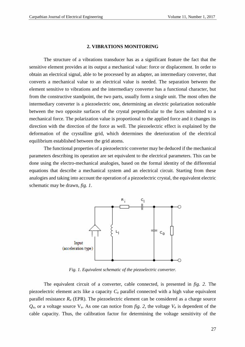
The functional properties of a piezoelectric converter may be deduced if the mechanical

parameters describing its operation are set equivalent to the electrical parameters. This can be

done using the electro-mechanical analogies, based on the formal identity of the differential

equations that describe a mechanical system and an electrical circuit. Starting from these

analogies and taking into account the operation of a piezoelectric crystal, the equivalent electric

schematic may be drawn, fig. 1.

Fig. 1. Equivalent schematic of the piezoelectric converter.

The equivalent circuit of a converter, cable connected, is presented in fig. 2. The

piezoelectric element acts like a capacity Ca parallel connected with a high value equivalent

parallel resistance Ra (EPR). The piezoelectric element can be considered as a charge source

Qa, or a voltage source Va. As one can notice from fig. 2, the voltage Va is dependent of the

cable capacity. Thus, the calibration factor for determining the voltage sensitivity of the


28

convertor, must take into account the connection cable. If different cables than those specified

are used, correction coefficients depending on the capacity of the new cable must be introduced,

or a new voltage sensitivity must be considered.

An important parameter for achieving a proper operation of the converters is the

transverse sensitivity, determined versus the applied acceleration under square angles with

respect to the main axis. It is expressed in percent versus the load sensitivity or the voltage,

measured with respect to the main direction. It must be mentioned that the maximum sensitivity

is not obtained versus the main direction of the piezoelectric crystal, in which, maximum and

minimum directions of sensitivity exist. Usually, the minimum sensitivity direction is labelled

on the device housing. For an ideal piezoelectric material, the transverse sensitivity is zero, but

in reality, due to the fabrication imperfections, it differs from zero, reaching three percent of

the main sensitivity. The dependency of the transverse sensitivity versus frequency is depicted

in the catalog sheet of the producer.

Fig. 2. Equivalent schematic of the voltage generator.

A special attention must be paid to the measurement of the chokes and of the transients,

since important errors may occur, like for instance the displacement error in relation to zero, or

the ringing error.

The displacement error in relation to zero is due to the phase nonlinearities generated in

the amplifier by the low frequency components of the real signal. These distortions don’t affect

the average value, but they can influence the accurate determination of the peak value. In order

to maintain these errors in certain imposed limits, it is compulsory that the inferior limit of the

preamplifier be lower than a value inverse proportional to a choke or to the period of a transient.

It is also recommended the use of acceleration type sensitive elements, because the integration

of a single choke in order to obtain velocity or displacement, introduces phase nonlinearities.


29

The displacement in relation to zero may be produced by the converter itself, especially

when high level chokes are applied, determining that only a fraction of the charge stored in the

piezoelectric element to be transmitted for measurement.

The ringing error occurs when the frequency spectrum of the choke contains frequency

components close to the mechanical resonance frequency. In order to make errors less than an

imposed value, a preamplifier and a low pass filter in the input are needed.

If the piezoelectric converters are used beyond the maximum temperature specified for

piezoelectric materials, the piezoelectric elements depolarize themselves, determining a

permanent loss of the charge and consequently the lowering of the sensitivity. The explanation

of this phenomenon consists in the modification of the electric permittivity of the material

versus temperature. An analysis regarding this phenomenon shows that the Rochelle salt can’t

be accepted as a piezoelectric sensitive material, due to its instable properties versus the

temperature. There are also several varieties of barium titanate having a different behavior

versus temperature. Conversely, the lead zirconate-titanate has practically the same stability as

the quartz. One solution in increasing time stability of the sensitivity versus time and

temperature consists in the artificial aging.

3. ANALOG TO DIGITAL CONVERSION

Monitoring the operating conditions of an electric machine may estimate the moment of

the maintenance process. A periodic monitoring of the operation parameters of the equipment,

using analysis vibration techniques, makes possible the detection of the problems associated to

the wind electric generators. Consequently, the possible issues can be previewed and detected

fast enough, in order to draw a repair planning, instead of a preventive maintenance. Measuring

vibrations in different locations of the wind electric generator and tracking their intensity in

time, represent a reliable and efficient approach, indicating the weary state of an equipment and

its time involution. Using a vibrometer permits the visualization of the measurement results,

directly in situ. Modern vibrometers have the possibility to store the measurement results in the

internal memory of the vibrometer in different equipment, USB connected thereto. The saved

results of the measurements can be downloaded later through a communication port and a RS

232 serial interface or a USB interface, provided at the new generation of vibrometers.

Connecting the vibrometer to a PC and using one of the available communication ports,

permit also to download and save the data. In order to use a USB communication port, a

dedicated driver, delivered by the producer, is compulsory to be installed. For the serial

communication port, RS232, the special drivers are not needed. The data being stored in the

PC, the user can export them in special application, able to view and compare them with other

previous similar data.


30

Each producer of measurement equipment has developed applications, which are

working together with the equipment in order to extract and export data. These applications are

most often closed source, meaning a compiled ready version, unmodifiable by the user for his

special needs. The closed source applications save data in specific files. Thus, the user is forced

to use the applications provided by the manufacturer.

Some vibrometers have the ability to transmit the measured and amplified signals to a

special analogic port in order to be processed by further equipment. This signal can be taken

over by an acquisition board, that converts an analog signal into a digital one.

Such an acquisition board is 232M1A0CT [6]. The acquisition board, fig. 3, has eight

analog inputs and ten digital inputs. The analog inputs are unipolar and admit voltages between

0 and 10 Vd.c. The board is supplied by a direct current voltage, in the range from 7.5 V to 24

V and a direct current of 50 mA.

The communication with the monitoring system is made via a RS232 interface. The

transmission is made in duplex synchronous mode, each transmitted or received word

containing eight data bits, one parity bit and one start/stop bit.

The interface RS232 permits the connection of the monitoring system at a maximum distance

of 15 m.

Communication through the RS232 port uses three wires: the first for transmitting data,

the second for receiving data and the third for grounding. Between the transmitting and

receiving wires and the ground, one can measure values between -8 V and +12 V, respectively

+8 V and -12 V. The more complex applications impose a confirmation method of the

transmitted data, for preventing the buffer overflow and for verifying the equipment status as

well.

In order to control the flux of data between the two equipment the standard words

Request to Send-RTS and Clear to Send-CTS are used. The words Data Set Ready-DSR and

Data Terminal Ready-DTR are the most used words to call and to answer to the interrogations.

Fig. 3. The acquisition board is 232M1A0CT


31

4. REMOTE DATA TRANSMITTING TECHNIQUES

If the monitoring station is situated at a distance of more than 15 m related to the

measuring point, the following methods of data transmission can be used:

Wireless data transmission;

Optical fiber data transmission;

UTP cable data transmission.

Wireless grids represent networks of interconnected equipment by radio waves, infrared

waves and other wireless methods. In the last years, the wireless techniques have greatly

developed, being a reliable and simple alternative solution to cable links. Wireless connections

become more and more popular, while they solve problems that appear in the case of large grids

of several devices. Modern technologies are able to interconnect equipment situated at small to

large distances.

A Wireless Local Area Network- WLAN represents a communication system

implemented like an extension or an alternative to a cabled LAN, in a building or a campus,

combining connectivity at high speed, providing the mobility of the users in a more simplified

configuration. Obvious advantages, like mobility, flexibility, simple commissioning, reduced

maintenance costs and scalability have imposed WLAN as a more often used solution.

There are two types of wireless transmitting/receiving equipment:

Base Stations;

Subscriber Units.

The base stations antennas have usually a wide angle, ranging from 60 degrees to 360

degrees capable to assure the connectivity of all the customers in a certain area. The base

stations can be connected to an optical fiber cable network or radio relays.

The antennas of the subscriber units have a much narrower angle and therefore they

have to be oriented towards the base station.

Optical fibers are used on large scale in telecommunications, permitting long distance

transmissions having higher band widths than other media communication. Through optical

fibers, a signal is transmitted with reduced losses, being immune to electromagnetic

interference as well. Consequently, they are used instead of the electrical cables, in lighting

technique and images transmission, permitting the visualization in narrow areas. Some of

special designed optical fibers are used in several applications, including sensors and laser

applications. The waveform in the optical fibers is directed through the core of the fiber using

the total reflection, which leads to a waveguide behavior of the optical fiber. The fibers that

support several propagation or transverse modes are the so called multimode fibers – MMF,

and the fibers that support only one propagation mode are the so called single mode – SMF.

The multimode fibers have in general a larger diameter of the core and are used in short distance


32

communications and in applications in which a higher transfer of power is needed. The single

mode fibers are used in communications at distances over 550 m.

The junctioning of the optical fibers is a more complex process than the junctioning of

the conventional cables. The extremities of two optical fibers cables must be properly prior

prepared and afterwards welded using an electric arc technique. Special connectors, suitable for

flexible connections, are used.

Data transmission via optical fiber is performed using both types of fiber, both having

the same diameter of 0.12 mm.

The multimode fiber has a larger core diameter, usually of 62.5 µm, but there are also

optical fibers having the core diameter of 50 µm, used together with LED lighting sources,

having wavelengths of 850 nm and 1300 nm for low speed connections and with laser sources,

having wavelengths of 850 nm and 1300 nm for high speed connections of several gigabytes

per second.

The single mode fiber has a thinner core, of only 9 µm, and the waveform is transmitted

in one flux. It is used together with laser sources having wavelengths between 1300 nm and

1550 nm.

In order to connect the acquisition board with the monitoring station via optical fiber, a

pair of RS232 and RS485 converters is needed. The connection between the acquisition board

and the monitoring station could be achieved with lower costs using a UTP cable. This

connection is possible only for distances of maximum 15 m, without ancillary equipment, with

a maximum baud-rate of 115200 bauds/s. If the baud-rate is lower, the equipment can be

connected at a longer distance. For instance, for a baud rate of 9600 bauds/s the possible

connection distance becomes 150 m.

In order to maintain a high value baud-rate, a current loop converter can be used, fig. 4.

The converter performs the conversion between the RS232 serial interface to the current loop

of 20 mA or 60 mA. This device need an external supply source as well.

Two such converters are needed. The first is needed for transmitting signals from the

RS232 port of the acquisition board and the second for receiving data at the RS232 port of the

acquisition board.

Fig. 4. RS232 to current loop converter.


33

5. EXPERIMENTAL SETUP

The experimental setup using a UTP cable connection is composed of the following

elements:

Piezoelectric transducer Dytran 3100B 6221;

Sound and vibrations analyzer Svan 912 AE;

Oscilloscope Fluke 196;

Acquisition board 232M1A0CT;

Calibration generator vibrometer RTF.

The piezoelectric transducer is connected via a coax cable to the input port of the sound

and vibrations analyzer, Svan 912AE. The analyzer is provided with a converter, that converts

the electrical charge to a voltage, which permits the charge measurement. The converter can be

also connected to analog measurement instruments via a BNC connector. This feature is used

in the experimental setup to connect an oscilloscope. fig 5, represents a picture of the

experimental setup.

Fig. 5. Experimental setup, simulating the wind turbines vibrations monitoring.

Fig. 6. The sinusoidal vibration oscillogram.


34

The piezoelectric transducer is mounted on the vibrations source using a magnetic pad,

consisting of a permanent magnet assuring the transmission of the vibration generated by the

undistorted source.

The vibrations source is provided with a control element which is able to modify the

vibrations amplitude. Using the vibrations source, the normal operation of the wind generator

is simulated.

Fig. 7. Amplitude versus time spectrum at the output of the acquisition board.

Both the oscillogram of the sinusoidal vibration, fig. 6, and the amplitude versus time

spectrum, fig. 7, highlight a normal operation of the wind generator. Notice that the output of

the acquisition board has only a positive component, due to the fact that the input of the

acquisition board admits only positive voltages, ranged between 0 Vd.c. to 10 Vd.c.

In order to simulate the faulty situation, the vibration generator generates also chokes,

fig. 8, presenting non-sinusoidal vibrations. Fig. 9 depicts situation in which the chokes

determine the monitoring system to signal a faulty situation.

Fig. 8. The non-sinusoidal vibration oscillogram.


35

Fig. 9. The amplitude-time spectrum at the output of the acquisition board in case of a fault.

6. CONCLUSIONS

In order to simulate a faulty operation, a variable vibrations source is used, the control

circuit having the possibility to determine the generation of chokes, that simulate the operation

of the wind turbine in case of fault.

The experimental results depicted in figs. 6-9 highlight the role of the acquisition board

in the monitoring equipment. The measured values can be saved in CVS type files, a format

that doesn’t need special drivers for being open and read.

Using an acquisition board capable monitoring more piezoelectric transducers mounted

on the main elements of a wind generator, exhaustive information, during the operation time of

the wind generator can be obtained. Therefore, the faults of these elements may be detected in

incipient stages. Consequently, a repair planning can be drawn, more effective than applying

simple preventive maintenance measures. Consequently, major faults that can make the wind

generator inoperable could be avoided.

REFERENCES

[1] W. Musial, S. Butterfield, B. McNiff, Improving Wind Turbine Gearbox Reliability, European

Wind Energy Conference ,Milan, Italy, May 7–10, 2007.

[2] http://www.bksv.com

[3] Paul D, Detection of change in process using wavelets, Proc. IEEE-SP Int. Symp. Time-

Frecquency and Time Scale Analysis, 174-177, 1994.

[4] Ladd M.D and Wilson G.R., Proportional bandwidth properties of fault indicating tones in a ball

bearing system, the 28-th Asilomar Conf. Signals, Systems and Computer, 45-49, 1994.

[5] A.R. Mohanty et al., Fault detection in a multistage gearbox by demodulation of motor current

waveform, IEEE Trans. Industrial Electronics, vol. 53, no.4, pp. 1285-1297, August 2006.

[6] *** www. Integrity Instruments Inc.com

http://www.bksv.com/


36


37

A METHOD FOR DENOISING IMAGE CONTOURS

Ovidiu COSMA

Technical University of Cluj-Napoca, North University Center of Baia Mare

[email protected]

Keywords: edge detection, noise removal

Abstract: The edge detection techniques have to compromise between sensitivity and

noise. In order for the main contours to be uninterrupted, the level of sensitivity has to be

raised, which however has the negative effect of producing a multitude of insignificant

contours (noise). This article proposes a method of removing this noise, which acts directly

on the binary representation of the image contours.

1. INTRODUCTION

Contour detection is a fundamental technique of image processing. Edges and contours

play a key role in the human visual system and underpin computer vision applications, such

as robot guidance, automatic inspection, process control, and medical applications. Contours

play a key role in the perception of images. It is often possible to understand the content of

an image that has been reduced to a few basic lines. Consequently, we can conclude that a

major part of information in an image lays in objects contours.

Despite the importance of the subject, at present there is no known technique of tracing

perfect contours. This is due to the fact that there is a need to compromise between the

following two complementary features: thin and uninterrupted contour lines and the absence

of false contours (no noise).

2. METHODS OF EDGE DETECTION

The contours in an image are made up of pixels for which brightness changes steeply

after a certain orientation. The first contour detection methods are based on gradients, which

are calculated using first-order derivatives in horizontal and vertical directions [1, 2]. If we


38

look at a digital image as a function of two variables 𝑓(𝑥, 𝑦), then the gradient vector is

defined according to relation (1), and the gradient magnitude is defined in relation (2).

∇𝑓(𝑥, 𝑦) =

[ 𝜕𝑓

𝜕𝑥(𝑥, 𝑦)

𝜕𝑓

𝜕𝑦(𝑥, 𝑦)

]

(1)

|∇𝑓(𝑥, 𝑦)| = √(𝜕𝑓

𝜕𝑥(𝑥, 𝑦))2 + (

𝜕𝑓

𝜕𝑦(𝑥, 𝑦))2 (2)

The points on the contours are those for which the magnitude of the gradient exceeds

a certain threshold. A simple binarization operation can be applied for tracing the contours.

The following two filters, known as Roberts filters [1, 2], can be used to estimate the gradient.

They determine diagonal contours, but are not very sensitive to orientation. Because they are

as small as possible, they can detect the finest contours.

𝐻1𝑅 = [

0 1−1 0

] , 𝐻2𝑅 = [

−1 0 0 1

] (3)

Any contouring technique has to deal with noise-related issues, because they can be

mistakenly interpreted as edges. For this reason, it is preferable to apply a smoothing filter

before edge detection [1, 2]. Any smoothing filter would solve this problem, but it is

preferable one that does not affect too much the edges. The Gaussian filter defined in relation

(4) is frequently used because it is configurable by standard deviation 𝜎, which determines

the width of the bell.

𝐺(𝑥, 𝑦) =1

2𝜋𝜎2𝑒

−𝑥2+𝑦2

2𝜎2 (4)

This smoothing step may be omitted if the filters that are used calculate the average

values of the gradient. The next two filters (Sobel) calculate at each step the gradient average

on 3 lines, respectively on 3 columns [1-3]. Figure 1.b shows the contours of the image in

figure 1.a, drawn by applying the Sobel filters, followed by a thresholding operation.

𝐻𝑥𝑆 = [

−1 0 1−2 0 2−1 0 1

] , 𝐻𝑥𝑆 = [

−1 −2 −1 0 0 0 1 2 1

] (5)


39

The main problem of all the gradient based techniques is the fact that they rely on the

first-order derivative, which is nonzero in ramps. For this reason, they draw relatively thick

contours and artificial thinning techniques are required. To solve the problem, edge detection

techniques based on the second order derivative were developed [1, 2]. They draw thinner

contours, but they have the disadvantage of doubling roof edges.

The Laplace operator for an image 𝑓(𝑥, 𝑦) is obtained by summing the second order

derivatives calculated in the horizontal and vertical directions.

∇2𝑓(𝑥, 𝑦) =𝜕2𝑓

𝜕𝑥2(𝑥, 𝑦) +

𝜕2𝑓

𝜕𝑦2(𝑥, 𝑦) (6)

Figure 2.a was generated using the Laplace operator followed by thresholding. The

Laplacian filters can detect fine edges, but they have a high sensitivity to noise. As a result, a

pre-smoothing operation is required. For efficiency, the two operations (smoothening and

edge detection) can be combined into a single one using a Laplacian of Gaussian (LoG) filter

that can be calculated based on the following relation:

𝐿𝑜𝐺(𝑥, 𝑦) = −1

𝜋𝜎2[1 −

𝑥2 + 𝑦2

2𝜎2] 𝑒

−𝑥2+𝑦2

2𝜎2 (7)

Figures 2.b and 2.c were generated using the LoG filter, with a standard deviation 𝜎

of 0.8 and 1.4 respectively.

An optimized contour detecting method known as the Canny operator is proposed in

[4]. The proposed method comprises the following steps:

1. Apply a Gaussian smoothing filter to the original image, for noise reduction.

2. Use the Sobel filters to determine both gradient magnitude and gradient

orientation.

3. Apply a contour-thinning algorithm that reduces all contours to one pixel

thickness. In the case of thick contours, only the pixel with maximum gradient

magnitude in the direction of the gradient orientation remains. All other pixels

will be removed from the contour.

4. To avoid discontinuous contours, a hysteresis thresholding algorithm is proposed.

This algorithm uses two thresholds. In the first step, a higher threshold is used,

based on which the pixels belonging to contours are set. In the second step, a

lower threshold is used, based on which other pixels are added to the contours,

provided they are connected to the pixels selected in the first step.

The contour image in figure 1.c was generated by applying the Canny operator on the

image in figure 1.a.


40

a.) Original image b.) Sobel filter c.) Canny operator

Fig. 1. Original image and contour images

a.) Laplacian filter b.) LoG filter, 𝜎 = 0.8 c.) LoG filter, 𝜎 = 1.4

Fig. 2. Image contours

3. RECENT RESULTS

A Laplacian of B-spline operator for edge detecting is proposed in [6]. The authors

claim that the new operator outperforms the Canny and the LoG operators in the case of noisy

images. In [7] is presented a new method for detecting the boundaries of homogenous regions.

The method is based on gradient intensity and texture variations. The wavelet transform is

used for calculating a texture representation. A method based on non-linear filtering for

structure preserving noise reduction and edge / corner detection is presented in [8]. A multi

resolution edge detection technique is proposed in [9]. For increasing accuracy, the algorithm

performs edge pattern analysis. A parallel implementation that runs in real-time is presented.

In [10] is presenred a new contour detection algorithm that is based on quantum entropy. The

efficiency of the method is demonstrated using different examples. The performance is

evaluated using the peak-signal-to-noise ratio. An edge detecting method based on fractional

Fourier transformation is presented in [11]. The authors show that the proposed method

performs better than classical methods in terms of resilience to noise. A method of contour

detection based on the Canny operator enhanced with an ant colony optimization algorithm


41

is presented in [12]. A new contour detection method for color images is presented in [13].

The method is based on the vector angle between adjacent pixels. An edge detection method

based on a logarithmic image processing model is presented in [14]. The author claims that

the proposed method performs better than the classical methods in the presence of noise. A

new contour detection method is proposed in [15]. The method is based on gradient

calculation, followed by a frequency domain filtering step.

A multiresolution contour detection method is proposed in [16]. The method is based

on Bayesian denoising and inhibition of the surroundings. The gradient is calculated at

different resolutions then the edges are denoised. In the surrounding inhibition step, the edges

that represent texture are recognized and suppressed. A technique based on local and global

analysis is proposed in [17]. The contour detection is performed by integrating the local edges

detected by filtering with a global saliency map. A histogram difference function is presented,

for estimating the probability of the pixels to belong to contours. A multi-scale morphological

edge detection algorithm for noisy images is presented in [18]. The key features of the

algorithm are robustness and accuracy. An evaluation of the linear methods for image contour

detection is presented in [19]. The methods are evaluated on basis of sampling errors, output

noise level, and computational complexity.

4. THE PROPOSED METHOD

Of all the filters for edge detection, the Laplacian filter has the most promising results,

but they are shadowed by the high level of noise. The only way to reduce noise is to raise the

binarization threshold, but this operation may cause important contours to be interrupted. The

LoG filter introduces an additional parameter that can adjust the noise level. This is the

standard deviation 𝜎 that controls the width of the Gaussian filter that performs the initial

smoothing operation. But unfortunately, the initial filtering does not completely solve the

problem. A large 𝜎 also affects the thickness of contour lines.

The proposed method is different from the existing ones by the fact that it acts at the

end (after the LoG filter and the thresholding operation), on the binary contour image. The

method operation is presented in figure 3.

image thresholding denoisingLoG filter

initial

contours

( I )

threshold

final contours

( F )

s minimum length

Fig. 3. Operation of the proposed method

The denoising block performs the following operations:


42

1. All the pixels of the final contours image ( F ) are initialized with white.

2. The initial contours image ( I ) is traversed along lines and columns. For each black pixel

encountered, the following processing is performed:

2.1. Initialize a list with the position of the pixel,

2.2. Change pixel color to white,

2.3. Add to the list all the black neighbors of the pixel, and their black neighbors, and

the black neighbors of their neighbours, etc. Change the color of all pixels added

to the list in white. The eight neighbors of the pixel on line y and column x are

shown in figure 4.

2.4. If the number of items in the list exceeds a certain threshold, then the color of all

the pixels in image F that are located in the positions indicated by the list elements

will be changed to black.

x-1 x x+1

y-1

y

y+1

Fig. 4. A pixel neighbors locations


The image in figure 1.a was used for demonstrating the performance of the method.

The images obtained after applying the LoG filter for different values of the standard

deviation 𝜎 are shown in figure 5. To avoid the interruption of important contours, a relatively

small threshold was chosen. This adds a lot of noise in the countours. The result of applying

the contour cleaning algorithm is shown in figure 6.

a.) 𝜎 = 0.6 b.) 𝜎 = 0.8 c.) 𝜎 = 1.4

Fig. 5. LoG filter contours


43

a.) 𝜎 = 0.6 b.) 𝜎 = 0.8 c.) 𝜎 = 1.4

Fig. 6. Cleaned LoG filter contours

For verifying the properties of the method, it was applied on a set of “standard images,

which are commonly used in literature. The test images are presented in figure 7. They were

taken from [20]. The contours of these images were drawn using the Sobel and Roberts filters,

the Canny operator and the proposed method. The results are presented in figures 8.1 and 8.2.

a.) Cameraman b.) Jetplane c.) Pirate d.) Blonde woman e.) Peppers

Fig. 7. Set of test images

a.) Sobel filter b.) Roberts filter c.) Canny operator d.) Proposed method

Fig. 8.1. Comparison of the results


44

a.) Sobel filter b.) Roberts filter c.) Canny operator d.) Proposed method

Fig. 8.2. Comparison of the results

6. CONCLUSIONS

The method presented in this paper can be used to eliminate noise from contours

generated with the LoG filter, adding an additional optimization parameter: minimum length

(the minimum number of adjacent black pixels). This allows lowering the binarization

threshold, to avoid interrupting important contours. The proposed algorithm is relatively

simple and acts directly on the binary representation of the image contours. The contours


45

obtained in this way are clean and firm. They are visually superior to those obtained using

classical techniques.

REFERENCES

[1] Wilhelm J. Burger, Mark J. Burge, Principles of Digital Image Processing, Springer, 2013.

[2] Rafael C. Gonzalez, Richard E. Woods, Digital Image Processing, Prentice-Hall, 2002.

[3] Irwin Sobel, History and definition of the so-called Sobel Operator,

https://www.researchgate.net/publication/239398674_An_Isotropic_3_3_Image_Gradient_Op

erator, (accessed 2017-05).

[4] John Canny, A Computational Approach to Edge Detection, IEEE Transactions on Pattern

Analysis and Machine Intelligence, Vol. 8, Issue 6, November 1986, pp. 679 – 698.

[5] D. Marr; E. Hildreth, Theory of Edge Detection, Proceedings of the Royal Society of London,

Series B, Biological Sciences, Vol. 207, No. 1167, pp. 187-217, 1980.

[6] Dongqing Xu, Xiuyou Wang, Gang Sun, Huaimin Li, Towards a novel image denoising method

with edge-preserving sparse representation based on laplacian of B-spline edge-detection,

Multimedia Tools and Applications, 2015.

[7] Nasser Chaji, Hassan Ghassemian, Texture-Gradient-Based Contour Detection, Journal on

Applied Signal Processing, pp. 1–8, 2006.

[8] Stephen M. Smith, J. Michael Brady, SUSAN—A New Approach to Low Level Image

Processing, International Journal of Computer Vision Vol. 23, Issue 1, pp. 45–78, 1997.

[9] Bo Jiang, Real-time multi-resolution edge detection with pattern analysis on graphics

processing unit, Journal of Real-Time Image Processing, pp. 1-29, 2014.

[10] S. Abdel-Khalek, Gamil Abdel-Azim, Z. A. Abo-Eleneen, A.-S. F. Obada, New approach to

image edge detection based on quantum entropy, Journal of Russian Laser Research, Volume

37, Number 2, March, 2016.

[11] Sanjay Kumar, Rajiv Saxena, Kulbir Singh1, Fractional Fourier Transform and Fractional-

Order Calculus-Based Image Edge Detection, Circuits, Systems, and Signal Processing, Vol.

36 Issue 4, April, pp. 1493-1513, 2017.

[12] P. Hinduja, K. Suresh, B. Ravi Kiran, Edge Detection on an Image Using Ant Colony

Optimization, Proceedings of the Second International Conference on Computer and

Communication Technologies, pp. 593-599, September 2015.

[13] Young-Hyun Baek, Oh-Sung Byun, Sung-Ryong Moon, Deok-Soo Baek, Edge Detection in

Digital Image Using Variable Template Operator, International Conference on Knowledge-

Based and Intelligent Information and Engineering Systems, pp. 195-200, 2005.

[14] Guang Deng, Differentiation-Based Edge Detection Using the Logarithmic Image Processing

Model, Journal of Mathematical Imaging and Vision Vol. 8, pp. 161–180, 1998.

[15] Qu ZhiGuo, Gao YingHui, Wang Ping, Wang Peng, Tan XianSi, Shen ZhenKang, Contour

detection improved by frequency domain filtering of gradient image, Science China Information

Sciences, Volume 57, Issue 1, January, pp. 1–11, 2014.

[16] Giuseppe Papari, Patrizio Campisi, Nicolai Petkov, Alessandro Neri, A Biologically Motivated


46

Multiresolution Approach to Contour Detection, Journal on Advances in Signal Processing,

Vol. 2007.

[17] Hong Cheng, Lin Chen, A Holistic Approach for Efficient Contour Detection, Journal of

computer science and technology, Vol. 29, Issue 6, pp.1038-1047, November 2014.

[18] Tang Zhengjun, Song Jianshe, A multi-scale morphological approach to SAR image edge

detection, Journal of electronics, Vol. 17, No. 3, July 2000.

[19] M. Yu. Khomyakov, Comparative Evaluation of Linear Edge Detection Methods, Pattern

Recognition and Image Analysis, Vol. 22, Issue 2, June, pp. 291–302, 2012.

[20] http://www.imageprocessingplace.com/root_files_V3/image_databases.htm, (accessed 2017-

07).

http://www.imageprocessingplace.com/root_files_V3/image_databases.htm


47

TESTING SOLUTIONS OF THE PROTECTION SYSTEMS PROVIDED

WITH DELAY MAXIMUM CURRENT RELAYS

Horia BALAN, Mircea I. BUZDUGAN, Ionut IANCAU, Liviu NEAMT

Technical University of Cluj-Napoca, Romania

[email protected]

Keywords: power system protection, current relays

Abstract: Relay protection is one of the main forms of automation control of electro energy

systems, having as primary aims fault detection and disconnection of the faulty element in

order to avoid the extent of damages and the as fast as possible recovery to the normal

operation regime for the rest of the system. Faults that occur in the electro energy system

can be classified considering on one hand their causes and on the other their types, but in

the vast majority of cases the causes of the faults are combined. Further, considering their

nature, faults are classified in faults due to the insulation’s damage, in faults due to the

destruction of the integrity of the circuits and faults determined by interruptions. With respect

to their nature, faults are short circuits, earthing faults and phases interruptions. At the same

time, considering their type, faults are divided in transversal and longitudinal ones. The

paper presents a testing solution of the delayed maximal current relays using a T3000 ISA

Test measuring equipment.

1. INTRODUCTION

A very important issue of the a. c. power grids consists in defining the command, control

and protection strategy, meant to assure the normal, safe and stabile operation of the system.

There are several elements which must be considered in the choice of the protection

system. The design and the choice of a protection system implies the knowledge of the faults

that may appear in electric grids. From the point of view of the effects, immediate or delayed

in time, these faults may be of a greater or lesser intensity. Current relays represent the primary

protection in the distribution systems. The development of electronic devices, replaced the old

electromechanical technology, used in the first generations of protective relays, with the static


48

technology. However, static relays present several drawbacks, since analog circuits are very

sensitive to electromagnetic interference. On the other hand, the magnitudes of the voltage and

the currents are limited in analog circuits, affecting the relay sensitivity.

Embedding a microprocessor in the architecture of a relay, which emulate the function

and the logic of a relay dates from the early eighties.

Digital relays represent sophisticated equipment, having multiple uses and having the

possibility of recording signals during the fault, monitoring and communicating with other

relays in the grid. Digital relays use dedicated microprocessors for processing digital signals,

being therefore more rapid, and efficient, but maintaining in the same time their economic

advantage.

Most of situations, it is impossible to investigate the above mentioned features in a real

case of a system, due to different economic, functional of security impediments. Therefore,

several approaches and equipment have been developed, in order to overcome these

deficiencies: e.g. real time digital simulators (RTDS), reversible real time digital simulators and

software packages for modeling protective relays [1].

Digital models of the protective relays offer an economic and reliable alternative in the

analysis of relays performance and of the protection systems. At the same time, they permit a

detailed analysis of the performance at the level of each internal module. Implementation of

new algorithms is improved using modeling, which offers the possibility of settings and

corrections, before testing the prototypes and launching the production process. For more

specific problems, the use of the models offers the possibility of novel solutions, if the usual

configurations are not satisfactory.

2. CURRENT PROTECTION

The principle, consisting in the protection of the overcome of the limit values of the

current, was the basis of the early protection systems. Starting from this basic principle, step

maximum current protection systems have been developed. For an accurate operation of these

relays, one must know the fault currents in each element of the grid [2, 3, 4].

The compulsory data for the relay settings are:

the wiring diagram of the protected system, consisting in the protection relays

and the associated current transformers;

the impedances of the elements of the system (generators, transformers,

transmission lines);

minimum and maximum values of the short circuit currents in each protection

location;

starting currents of electric motors;

maximum load current in each protection location;


49

the decay curves of the fault current supplied by the generators;

current transformers characteristics.

Fig. 1. Maximum current protection schematics.

The current relay settings must be checked in the first instance for the maximum value

of the short circuit current. The reaction time must be minimum. Afterwards, the operation of

the relay for minimum short circuit current must be checked. The reaction time must be

satisfactory.

The wiring diagram of a maximum current protection for a radial network power system

is depicted in fig. 2, where the bus insulator is denoted by SB, the line insulator, by SL, the

breaker by I, the current transformer by TC and finally by I> the maximum current relay.

The main devices composing this protection system are the maximum current relays and

the current transformers.

The tripping condition of the relay is:

c pI I (1)

where Ic represents the current in the surveyed circuit and Ip the tripping value of the relay, with

respect to the primary winding of the current transformer. Note that this protection acts in a

short circuit situation (instantaneous tripping with breaking) and doesn’t fit for protection

against overloads. The overload protection is also a current protection, but a delayed one. The

delay is needed for discriminating between transient and permanent overloads, the overloads

effects on the elements of the system being delayed in time.

Fig. 2. Overload protection relay schematics.


50

Note that the contacts of the both relays, the maximum current relay I> and the time

relay, perform a logic AND function. Consequently, the tripping of the breaker appears only if

the current in the circuit overcomes the set value Ip and the duration tc exceeds the delay time

tp:

andc p c pI I t t (2)

Maximum current relays may present an independent characteristic curve, when the

tripping time does not depend on the magnitude of the fault current, or a dependent one, when

the tripping time depends on the magnitude of the surveyed circuit (which is a multiple of the

set current). Consequently, this type of protection is characterized by the following features:

the maximum current protection is the simplest and the cheapest protection

(minimum number of components);

the settings are pretentious and difficult to achieve in applications;

readjustments and even relocating are needed in case of system modifications.

Protection must be selective in order to isolate the faulty area, leaving unaffected the

rest of the system. In this respect, the protection device located nearest the faulty location must

trip (i.e. the nearest fuse or breaker).

The correct coordination and the selectivity of the current protection may be achieved

using several methods. The main possibilities in achieving selectivity are based on the following

discrimination methods:

discrimination by time;

discrimination by current;

discrimination fault direction;

discrimination by both time and direction;

discrimination by both time and current.

3. SECONDARY CURRENTS INJECTION DEVICE T 3000

A short circuit in the energy system imposes the isolation of the fault location with

respect to the source, using commutation equipment. The electric arc occurring between the

contacts, following the deionizing processes, determines a quick wearing of these equipment.

If the short circuit duration is reduced, the protection system doesn’t determine the

disconnection, through the maximal delayed current relays.

The operation norms of the maximal delayed current relays impose that at several time

intervals, the protection characteristics should be tested and set at the imposed values.

Checking the protective relays is made in laboratory, using secondary injection

equipment (the authors of this paper have used the T/3000 [7, 8, 9] equipment, a complex

verifying kit , fig. 3, permitting tests on all types of relays which can be tested on monophasic


51

faults, respectively all other possible tests on voltage and current transformers, on energy meters

and on transducers as well.

The basic function of the equipment T/3000 is to generate currents and voltages,

depending on the type of test, which is set on the LCD display.

The test results are stored in the internal memory of the equipment. These results can be

subsequently transferred to a PC.

The equipment is provided with three generators:

the main generator, having six outputs: high value alternating current, low

value alternating current, low value direct current, current impulses, high

alternating voltage source and low alternating voltage source;

an auxiliary alternating voltage generator, generating an independent voltage

phase adjustable;

an auxiliary direct current generator used to feed relays under test.

All outputs are adjustable and metered on the large graphic LCD display. With the multi-

purpose control knob and the graphic LCD display it is possible to enter the MENU mode that

allows to control all functions and makes T3000 the most powerful testing device, with manual

and automatic capabilities and with the possibility to transfer test results to a PC via the RS232

interface.

Other key features of the equipment are:

oscilloscope function, permitting to display the measured current and voltage

waveforms;

other two independent measurement inputs for current and voltage, both with

High and Low inputs, permitting the measurement of the output of current and

voltage transformers and of any other sources;

a print option of the saturation curve of the current transformer and other test

results;

an auxiliary output contact that follows Start and Stop inputs, allows simulating

the circuit breaker.

Fig. 3. Secondary currents injection kit T 3000.


52

All the outputs of the T3000 kit are measured continuously. The waveform display

function is useful in the case of distorted current or voltage.

In order to test the relays, it is important to use the set function of the injected power,

due to the fact that the power of the nowadays relays is reduced. Because the current output is

a voltage generator with low impedance, the adjustment of the low currents or of the injected

currents on reduced loads is difficult because the operation in the initial area of the adjustment

device is needed. The solution consists in reducing the available power in order to achieve a

desired precision. Consequently the maximum voltage is reduced with a suitable factor.

The operator has different possibilities that permit to perform tests according to the

characteristics of the relays. Some parameters, unused for a certain test are however visualized

and saved. For instance, the auxiliary alternating voltage is also saved when a maximum current

relay is saved, even though this function is not used.

For testing the transformers, there is a window for each type of test and the testing

parameters are visualized and saved.

Each setting can be saved in the memory having the possibility to be reused afterwards.

A fix number of tests can be saved and reused, the initial setting being that corresponding to

the fault. The settings are continuously saved in the memory of the equipment, new settings

being stored at the same address after the confirming requirement. In normal use, only the

access to the standard settings is possible.

During the test, in the internal memory of the equipment can be saved up to 500 different

tests. When a test is finalized, the settings along with the corresponding results can be stored in

a personal computer where the X.PRO-3000 software is installed, which permits the

revisualization of the results. When a PC is connected to the T3000 kit during the tests, the

settings are available on the X.PRO-3000 interface.

Together with X.PRO-3000, the TDMS software is a powerful software package

providing data management for acceptance and maintenance testing activities. Electrical

apparatus data and test results are saved in the TDMS database for historical results analysis.

TDMS software organize test data and results for the majority of electrical apparatus tested with

ISA test sets and related software. TDMS software controls and provide data acquisition from

all ISA Test.

TDMS has a built-in report editor that allows to generate professional test report for a

single test object, for a group of tested devices or for an entire substation. It can create

customized report or use standard forms. TDMS tests report can be exported in MS Office

(Word and Excel), PDF or RTF formats.

TDMS is the control platform to run all ISA test software. Test programs, calibration,

firmware, software upgrade and languages are all managed from TDMS.

The TDMS software platform allows the user to select easily and quickly the most

appropriate software package for the required application. TDMS test software uses an open

architecture easily expandable with additional software modules at any time.


53

TDMS package can be used to test any protective relays in: power generation plants,

distribution and transmission networks and industry.

Manual control module has the following main characteristics:

Intuitive graphic interface;

Virtual front panel control;

Graphical vector control;

Ramp test: sequence of tests with ability to ramp any parameter up or down at

the same time;

Threshold test: automatic determination of threshold (current, voltage,

frequency, phase angle);

Rate of change (gradient) tests of frequency, voltage, current, phase angle and

Vdc (Dx/Dt);

Sequence editor;

Test of distance relays with direct import of relay characteristics with RIO

Format.

Test of distance relays with simulation of all types of faults: single phase, two

phase, two phase to ground, three phase;

Report manager allows test report customization to user requirements;

Comrade Module permits:

Playing back transient signals and waveform generation;

Playing back transient signals from digital fault recorders and numerical relays;

Analysis of relay operating time;

Graphical view and replay of analog and binary signals;

Impedance locus display;

Scaling, cut, copy and paste of the analog signals.

The program Control Tab has a new layout, namely the relays Test Plan and Editor,

which gives the user the possibility to create and run different test plan for different

applications. The Plan Editor is available to create a test plan using predefined macro functions

available for any type of relays. This new feature is particularly useful for testing multifunction

relays.

The Test Plan can be associated to any relay in TDMS network structure and prior

execution define relay setting and characteristic.

The Test Plan can be run on a specified relay: the entire test plan can be executed and/or

the user can select the macros to execute on that relay according to its needs.

Finally, the Test Plan can be printed and saved automatically into the TDMS database.


54


Using the T3000 testing equipment the authors of the paper performed tests on several

relays and current transformers.

The results of the tests, are displayed in the most simple cases using the internal memory

using the section Results or using the software TDMS, fig. 4-7.

The Sequencer module is a software for determining the relays operating time and the

logical sequence of the event.

Overcurrent module for automatic testing of overcurrent relays, including all

the standard curves IEEE and IEC [5, 6];

Differential relays module, for automatic testing of differential relays

(transformers, generators and bus bars);

Line differential module, for automatic testing of line differential relays;

Directional module, for testing of earth directional relays;

Synchronizing module, for automatic testing of synchronizing devices with

three or six voltages control;

Swing Pro module, for testing power swing blocking and out of step function;

Multifunction relays, which can be tested easily creating customized test plans;

Harmonic generator module, allowing the creation of arbitrary harmonic

waveform.

Fig. 4. Maximal current time relay RTpC-1; Set to 2 s and 6 A.


55

Fig. 5. Maximal current time relay RTpC-1; Set to 4 s and 4 A.

Taking into account the fact that the maximal time current relays permit a continuous

setting of the timing, it is important that using the measuring kit to obtain an interdependent

characteristic, as that presented in fig. 8 for the RTpC-1 relay.

The maximal induction time relay are nowadays quite rarely used in protection systems,

due to the interdependent time-current characteristics. A better performances version is

represented by the protection scheme presented in fig. 2. The scheme is composed by a current

relay along with a time relay, presenting an independent characteristics time-current.

The test equipment T 3000 permits the separate check of the two components of the

protection system, the RC2 current relay and the RTPa-5 time relay, and in the same time

determines the error of the measured value related to the setted value.

Fig. 6. Maximal current time relay RTpC-1; Set to 8s and 8 A.


56

Fig. 7. Maximal current time relay RTpC-1; Set to 6s and 3 A.

5. CONCLUSIONS

Continuity in electric energy supply and the most rapid alleviation of the electric

systems faults, in order to recover to a normal operating regime of these systems, means mostly

a safe and a correct operation of the protective relays.

A key role in assuring these conditions have got the test equipment, used at the

commissioning and the maintenance of the protection devices from the transformer stations and

substations.

The choice of the appropriate measurement kit for verifying, testing, commissioning

and maintenance is essential and must be considered in its technic and economic aspects.

In the choice of the T 3000 ISA TEST, the pros of this equipment have been considered,

i.e. the checking possibility of all types of relays, of energy meters, of different transformers,

along with the measurements of the earth resistivity, several ohmic tests, etc.

Using an equipment T 3000, equipped with a TDMS CT-VT-PT module in the

measurements performed on a RTpC-1 induction relay, which have in their componence a

transformer with eight outputs, is very suitable because this module permits recalling previous

measurements saved in the internal memory of the equipment, displaying in real time the

measured values and the relay characteristics, fig. 8, and in the same time processing the results

of the measurements.

In the case of a maximal time – protection system having in its componence the a current

relay RC2 and the time relay RTPa-5, the software package TDMS permits the automated

computation of the errors and their storage in a graphic or a tabular form.


57

Fig. 8. Maximal current time relay RTpC-1, i(t) dependent.

It is however true that the tests for the mono phase faults are not sufficiently accurate.

For these type of faults a more suitable test equipment should be used (for instance a secondary

currents injection kit, like Mentor 3V3I [10]). This last kit can successfully replace the

equipment presented previously.

2

3

4

5

6

7

8

9

10

11

3 4 5 6 7 8 9 10 11 12 13 14 15 16 17 18Iac [A]

t[s]

8s şi 8A

6s şi 3A

2s şi 6A

4s şi 4A

Poly. (2s şi 6A)

Poly. (8s şi 8A)

Poly. (6s şi 3A)

Poly. (4s şi 4A)


58

REFERENCES

[1] Q. H. Wu, Z. Lu, T. Y. Ji, Protective Relaying of Power Systems Using Mathematical

Morphology, Springer-Verlag London Limited, 2009.

[2] J. L. Blackburn, T. J. Domin, Protective Relaying - Principles and Applications, Taylor & Francis

Group, LLC, 2007.

[3] W. A. Elmore, Protective Relaying. Theory and Applications Second Edition, Marcel Dekker Inc.,

2004.

[4] J. Lewis Blackburn, Protective Relaying, Marcel Dekker Inc., 1987.

[5] IET, Power System Protection: Volume 1 – Principles and Components - 2nd Edition, Electricity

Training Association, London 1995.

[6] IEEE, Standard Dictionary of Electrical and Electronics Terms, IEEE, Wiley Interscience, 1972.

[7] ISA, Test Substation Maintenance and Commissioning Test Equipment.

[8] *** www.isatest.com

[9] ISA, Test T3000 Test Set, The Substation Equiment Test Set.

[10] *** www.eurosmc.com

http://www.isatest.com/


59

DECLINE OF ACTIVE POWER LOSS BY IMPROVED MOTH-FLAME

OPTIMIZATION ALGORITHM

Lenin KANAGASABAI

Department of EEE, Prasad V. Potluri Siddhartha Institute of Technology,

Kanuru, Vijayawada, Andhra Pradesh -520007, India

[email protected]

Keywords: Improved moth-flame optimization, Levy flight, optimal reactive power, transmission loss

Abstract: In this paper, Improved Moth-Flame Optimization (IMFO) algorithm has been

proposed for solving Reactive power problem. Navigation method of moths in nature called

transverse orientation is the key inspiration of the moth-flame algorithm (MFO). By

maintaining a fixed angle with respect to the moon, Moths fly in the night and it’s an effective

mechanism for moths travelling in a straight line for long distances. Due to very slow

convergence and poor precision, an improved version of MFO algorithm based on Levy-

flight strategy has been proposed to solve the reactive power problem. The diversity of the

population can be increased by Levy-flight to overcome premature convergence in order to

reach the global optimal solution. This methodology improves the trade-off between

exploration and exploitation ability of moth-flame algorithm (MFO).The proposed Improved

Moth-Flame Optimization (IMFO) algorithm has been tested in standard IEEE 30,57,118

bus test systems and simulation results show clearly about the better performance of the

proposed algorithm in reducing the real power loss with control variables within the limits.

1. INTRODUCTION

To till date various methodologies has been applied to solve the Optimal Reactive Power

problem. Many types of mathematical methodologies like linear programming, gradient method

(Alsac et al., 1973; Lee et al., 1985; Monticelli et al., 1987; Deeb et al., 1990; Hobson, 1980;

Lee et al., 1993; Mangoli et al., 1993; Canizares et al., 1996) [1-8] has been utilized to solve the

reactive power problem, but those techniques found difficult in handling the constraints in the

reactive power problem.. After that various types of evolutionary algorithms (Berizzi et al.,

2012; Roy et al., 2012; Hu et al., 2010; Eleftherios et al., 2010) [9-12] has been applied to solve


60

the reactive power problem. But some algorithm good in exploration means, it lacks in

exploitation and few algorithm’s good in exploitation but lack in exploration. Speed of

convergence is poor for some algorithms even though they got good trade-off between

exploration and exploitation. In this paper, Improved Moth-Flame Optimization (IMFO)

algorithm has been proposed for solving Reactive power problem. Navigation method of moths

in nature called transverse orientation is the key inspiration of the moth-flame algorithm (MFO).

By maintaining a fixed angle with respect to the moon, Moths fly in the night [13] and it’s an

effective mechanism for moths travelling in a straight line for long distances. Due to very slow

convergence and poor precision, an improved version of MFO algorithm based on Levy-flight

strategy has been proposed to solve the reactive power problem. The diversity of the population

can be increased by Levy-flight to overcome premature convergence in order to reach the global

optimal solution. This methodology improves the trade-off between exploration and

exploitation ability of moth-flame algorithm (MFO).The proposed Improved Moth-Flame

Optimization (IMFO) algorithm has been tested in standard IEEE 30, 57,118 bus test systems

and simulation results show clearly about the better performance of the proposed algorithm in

reducing the real power loss with control variables within the limits.

2. OBJECTIVE FUNCTION

2.1. Active power loss

Main objective of the reactive power dispatch problem is to minimize the active power

loss and mathematically written by,

F = 𝑃𝐿 = ∑ gkk∈Nbr (Vi2 + Vj

2 − 2ViVjcosθij) (1)

where: F - objective function, PL – power loss, gk – conductance of branch, Vi and Vj are voltages

at buses i, j, Nbr - total number of transmission lines in power systems.

2.2. Voltage profile improvement

Objective function F has be rewritten to minimize the voltage deviation in PQ buses as

follows,

F = 𝑃𝐿 + ωv × VD (2)

where VD – voltage deviation, ωv- is a weighting factor of voltage deviation.


61

The Voltage deviation is given by:

VD = ∑ |Vi − 1|Npqi=1 (3)

where Npq - number of load buses.

2.3. Equality Constraint

The power balance equation with respect to the equality constraint of the problem is

written as follows:

PG = PD + PL (4)

where PG- total power generation, PD - total power demand.

2.4. Inequality Constraints

The inequality constraint with upper and lower bounds on the active power of slack bus

(Pg), and reactive power of generators (Qg) are written as follows:

Pgslackmin ≤ Pgslack ≤ Pgslack

max (5)

Qgimin ≤ Qgi ≤ Qgi

max , i ∈ Ng (6)

Upper and lower bounds on the bus voltage magnitudes (Vi) is given by:

Vimin ≤ Vi ≤ Vi

max , i ∈ N (7)

Upper and lower bounds on the transformers tap ratios (Ti) is given by:

Timin ≤ Ti ≤ Ti

max , i ∈ NT (8)

Upper and lower bounds on the compensators (Qc) is given by:

Qcmin ≤ Qc ≤ QC

max , i ∈ NC (9)

where N is the total number of buses, Ng is the total number of generators, NT is the total

number of Transformers, Nc is the total number of shunt reactive compensators.


62

3. MOTH-FLAME OPTIMIZATION (MFO) ALGORITHM

Moth-flame optimization algorithm is based on the simulation of the behaviour of moths

which has special navigation methods in night. Navigation method of moths in nature called

transverse orientation is the key inspiration of the moth-flame algorithm (MFO).

By maintaining a fixed angle with respect to the moon, Moths fly in the night and it’s

an effective mechanism for moths travelling in a straight line for long distances. Set of moths

is represented in a matrix N in the MFO algorithm. There is an array 𝑂N for all the moths, to

store the corresponding fitness values. Flames are other one of key components in the moth-

flame algorithm.

It is also assumed that there is an array 𝑂L for the flames, a matrix S similar to the moth

matrix is considered to store the corresponding fitness values.

Three-tuple in MFO algorithm defined as follows:

𝑀𝐹𝑂 = (𝑄, 𝐺, 𝐻) (10)

An arbitrary population of moths is created by the function Q. Q function mathematical

model is given is as follows:

𝑄: ∅ → {𝑁, 𝑂𝑁} (11)

Moths move around the exploration space on basis of G function. G function received

the matrix of N and returns its modernized one ultimately:

𝐺:𝑁 → 𝑁 (12)

When the termination criterion is satisfied H function returns true and it will be false

when termination criterion is not satisfied:

𝐻:𝑁 → {𝑇𝑟𝑢𝑒, 𝐹𝑎𝑙𝑠𝑒} (13)

MFO algorithm is defined as follows, with Q, G, and H, as the general framework:

N = ( );

When (N) is equal to false condition, then: N = (N)

End.

𝑃 Function is iteratively run after the initialization, until the H function returns true.

When simulating the behaviour of moths mathematically, with respect to a flame the


63

position of each moth is updated using the following equation:

𝑁𝑖 = 𝑆𝐿(𝑁𝑖 , 𝐹𝑙𝑗) (14)

The 𝑖th moth indicated by N𝑖, 𝑗th flame indicated by 𝐹𝑙𝑗, and 𝑆L imply the spiral

function.

Spirals are utilized by following conditions: (a) initial point of the Spiral’s should start

from the moth; (b) final point of the Spiral’s should be the position of the flame; (c) in the

search space fluctuation range of spiral should not exceed the space limit.

Considering these points, a logarithmic spiral is defined for the MFO algorithm as

follows:

𝑆𝐿(𝑁𝑖, 𝐹𝑙𝑗) = 𝐷𝑇𝑖 ∙ 𝑒𝑏𝑡 ∙ 𝑐𝑜𝑠(2𝜋𝑓𝑡) + 𝐹𝑙𝑗 (15)

Distance of the 𝑖th moth for the 𝑗th flame is indicated by 𝐷T𝑖, for defining the shape of

the logarithmic spiral 𝑏 is a constant, and 𝑡 is an arbitrary number in the range [−1, 1].

Calculation of 𝐷T is as follows:

𝐷𝑇𝑖 = |𝐹𝑙𝑗 − 𝑁𝑖| (16)

where N𝑖 indicate the 𝑖th moth, 𝐹l𝑗 indicates the 𝑗th flame, and 𝐷T𝑖 indicates the distance of the

𝑖th moth for the 𝑗th flame. Spiral flying path of moths described by Equation (16). The next

position of a moth is defined with respect to a flame by equation (16).

In the spiral equation the 𝑡 parameter defines how much the next position of the moth

should be close to the flame (𝑡 = −1 is the closest position to the flame, while 𝑡=1 shows the

farthest). Position updating in equation (15) requires the moths to move towards a flame, & it

lead to be trapped in local optima quickly.

Each moth is obliged to update its position using only one of the flames by equation

(15) to prevent trap in local optima. In the search space the position updating of moths with

respect to 𝑛 different locations may degrade the exploitation to reach best promising solutions.

An adaptive mechanism is provided to the number of flame to resolve degrade problem & it

done by following equation,

𝐹𝑙𝑎𝑚𝑒 𝑛𝑢𝑚𝑏𝑒𝑟 = 𝑟𝑜𝑢𝑛𝑑 (𝐾 − 𝑙 ∗𝐾−𝑐𝑛

𝐼𝑁) (17)

The current number of iteration is given by cn, maximum number of flames indicated

by K, and the maximum number of iterations by IN. Exploration and exploitation of the search

space is perfectly balanced by gradual decrement in number of flames.


64

Position of moths has been initialized

While (Iteration <= Max iteration);

By equation (17) update the flame number

𝑂N = Fitness Function (N);

If iteration = = 1

𝐹l = sort (N); 𝑂𝐹l = sort(𝑂N);

Else

𝐹l = sort (N𝑡 – 1, N𝑡); 𝑂𝐹l = sort(N𝑡−1, N𝑡);

End

For 𝑖=1:𝑛 ; For 𝑗=1:𝑑

Modernize 𝑟 and 𝑡

By equation (16) calculate 𝐷T using with respect to the corresponding moth

By equations (14) and (15) renew (𝑖, 𝑗) with respect to the corresponding moth

End End.

4. LEVY-FLIGHT

Animals look for food in arbitrary manner, as moving place to place. The choice of the

direction relies only on a mathematical model [15], which is called Levy- flight & it have been

applied to optimization problems which show its promising capability [14,15].Mathematically

exclamation, an easy version of Levy distribution can be defined as [14],

𝐿(𝑠, 𝛾, 𝜇) = {√

𝛾

2𝜋

0 𝑖𝑓 𝑠 ≤ 0

𝑒𝑥𝑝 [−𝛾

2(𝑠−𝜇)]

1

(𝑠−𝜇)3 2⁄ 𝑖𝑓 0 < 𝜇 < 𝑠 < ∞ (18)

where 𝛾 > 0 parameter is scale (controls the scale of distribution) parameter, μ parameter is

location or shift parameter. In general, Levy distribution should be defined in terms of Fourier

transform as follows [14],

𝐹(𝑘) = 𝑒𝑥𝑝[−𝛼|𝑘|𝛽], 0 < 𝛽 ≤ 2 (19)

where α is a parameter within [-1,1] interval and known as scale factor. By Levy flight, new-

fangled state of the particle is designed as [15],

𝑋𝑡+1 = 𝑋𝑡 + 𝛼 ⊕ 𝐿𝑒𝑣𝑦 (𝛽) (20)

α is the step size which must be related to the scales of the problem of interest.


65

In the proposed method α is arbitrary number for all dimensions of particles [14].

𝑋𝑡+1 = 𝑋𝑡 + 𝑟𝑎𝑛𝑑𝑜𝑚 (𝑠𝑖𝑧𝑒(𝐷)) ⊕ 𝐿𝑒𝑣𝑦(𝛽) (21)

The product ⊕ means entry-wise multiplications. A non-trivial scheme of generating

step size s samples are summarized as follows [14],

𝑋𝑡+1 = 𝑋𝑡 + 𝑟𝑎𝑛𝑑𝑜𝑚 (𝑠𝑖𝑧𝑒(𝐷)) ⊕ 𝐿𝑒𝑣𝑦(𝛽)~0.01𝑢

|𝑣|1 𝛽⁄ (𝑥𝑗𝑡 − 𝑔𝑏) (22)

where u and v are drawn from the normal distributions. That is [15],

𝑢~𝑁(0, 𝜎𝑢2) 𝑣~𝑁(0, 𝜎𝑣

2) (23)

with

𝜎𝑢 = {Г(1+𝛽)𝑠𝑖𝑛(𝜋𝛽/2)

Г[(1+𝛽)/2]𝛽2(𝛽−1)/2}1

𝛽⁄ , 𝜎𝑣 = 1 (24)

Here Г is standard Gamma function. While performing distribution by Levy flights [14]

is the value taken by the β parameter and it substantially affects distribution.

5. PROPOSED IMPROVED MOTH- FLAME (IMFO) OPTIMIZATION

ALGORITHM

Proposed IMFO algorithm‘s global search ability is strengthened using arbitrary walk

with help of Levy-flight to eliminate the weakness of MFO algorithm [13] Improved Moth-

flame algorithm (IMFO) for solving Reactive power problem given below.

Position of moths has been initialized

While (Iteration <= Max iteration) ; By equation (17) update the flame number

𝑂N = Fitness Function (N);

If iteration = = 1

𝐹l = sort (N); 𝑂𝐹l = sort(𝑂N);

Else

𝐹l = sort (N𝑡 − 1, N𝑡); 𝑂𝐹l = sort(N𝑡−1, N𝑡);

End

For 𝑖=1:𝑛 ; For 𝑗=1:𝑑


66

Modernize 𝑟 and 𝑡

By equation (16) calculate 𝐷T using with respect to the corresponding moth

By equations (14) and (15) renew (𝑖, 𝑗) with respect to the corresponding moth

End

For each search agent renew the position of the existing search agent by using Levy-flight

End

When Iteration = Iteration + 1;

End

6. SIMULATION RESULTS

In standard IEEE 30-bus, 41 branch system validity of proposed Improved Moth-Flame

Optimization (IMFO) algorithm has been verified and the system has 6 generator-bus voltage

magnitudes, 4 transformer-tap settings, and 2 bus shunt reactive compensators. 2, 5, 8, 11 and

13 are considered as PV generator buses, Bus 1 is taken as slack bus and others are PQ load

buses. Primary variables limits are given in Table 1.

Table 1. Primary Variable Limits (Pu)

List of Variables Minimum Maximum group

Generator Bus 0.95 1.1 Continuous

Load Bus 0.95 1.05 Continuous

Transformer-Tap 0.9 1.1 Discrete

Shunt Reactive Compensator -0.11 0.31 Discrete

In Table 2 the power limits of generators buses are listed.

Table 2. Generators Power Limits

Bus Pg Pgminimum Pgmaximum Qgminimum Qmaximum

1 96.00 49 200 0 10

2 79.00 18 79 -40 50

5 49.00 14 49 -40 40

8 21.00 11 31 -10 40

11 21.00 11 28 -6 24

13 21.00 11 39 -6 24

Table 3 shows the proposed Improved Moth-Flame Optimization (IMFO) algorithm

successfully kept the control variables within limits.

Table 4 narrates about the performance of the proposed Improved Moth-Flame

Optimization (IMFO) algorithm.


67

Fig 1 shows about the voltage deviations during the iterations and Table 5 list out the

overall comparison of the results of optimal solution obtained by various methods.

Table 3. After optimization values of control variables

List of Control Variables IMFO

V1 1.0512

V2 1.0434

V5 1.0297

V8 1.0382

V11 1.0735

V13 1.0529

T4,12 0.00

T6,9 0.01

T6,10 0.90

T28,27 0.91

Q10 0.10

Q24 0.10

Real power loss 4.2898

Voltage deviation 0.9090

Table 4. Performance of IMFO algorithm

Iterations 25

Time taken (secs) 7.89

Real power loss 4.2898

Fig. 1. Voltage deviation (VD) characteristics

0 5 10 15 20 25 30 0

0.2

0.4

0.6

0.8

1

1.2

1.4

1.6

Iterations

VD

IMFO (HIGH)) IMFO (MEDIUM) IMFO (LOW)


68

Table 5. Comparison of results

List of Techniques Real power loss (MW)

SGA(Wu et al., 1998) [16] 4.98

PSO(Zhao et al., 2005) [17] 4.9262

LP(Mahadevan et al., 2010) [18] 5.988

EP(Mahadevan et al., 2010) [18] 4.963

CGA(Mahadevan et al., 2010) [18] 4.980

AGA(Mahadevan et al., 2010) [18] 4.926

CLPSO(Mahadevan et al., 2010) [18] 4.7208

HSA (Khazali et al., 2011) [19] 4.7624

BB-BC (Sakthivel et al., 2013) [20] 4.690

MCS(Tejaswini sharma et al.,2016) [21] 4.87231

Proposed IMFO 4.2898

At that Improved Moth-Flame Optimization (IMFO) algorithm has been tested in

standard IEEE-57 bus power system. The reactive power compensation buses are 18, 25 and 53.

Bus 2, 3, 6, 8, 9 and 12 are PV buses and bus 1 is selected as slack-bus. The system variable

limits are given in Table 6.

The preliminary conditions for the IEEE-57 bus power system are given as follows:

Pload = 12.129 p.u. Qload = 3.069 p.u.

The total initial generations and power losses are obtained as follows:

∑PG = 12.471 p.u. ∑QG = 3.3160 p.u.

Ploss = 0.25875 p.u. Qloss = -1.2074 p.u.

Table 6. Variable Limits

Reactive Power Generation Limits

Bus no 1 2 3 6 8 9 12

Qgmin -1.4 -.015 -.02 -0.04 -1.3 -0.03 -0.4

Qgmax 1 0.3 0.4 0.21 1 0.04 1.50

Voltage And Tap Setting Limits

vgmin Vgmax vpqmin Vpqmax tkmin tkmax

0.9 1.0 0.91 1.05 0.9 1.0

Shunt Capacitor Limits

Bus no 18 25 53

Qcmin 0 0 0

Qcmax 10 5.2 6.1


69

Table 7 shows the various system control variables i.e. generator bus voltages, shunt

capacitances and transformer tap settings obtained after optimization which are within the

acceptable limits. In Table 8, shows the comparison of optimum results obtained from proposed

methods with other optimization techniques. These results indicate the robustness of proposed

approaches for providing better optimal solution in case of IEEE-57 bus system.

Table 7. Control variables obtained after optimization

Control Variables IMFO

V1 1.10

V2 1.039

V3 1.038

V6 1.027

V8 1.029

V9 1.006

V12 1.011

Qc18 0.0664

Qc25 0.200

Qc53 0.0476

T4-18 1.004

T21-20 1.043

T24-25 0.861

T24-26 0.876

T7-29 1.057

T34-32 0.879

T11-41 1.011

T15-45 1.030

T14-46 0.910

T10-51 1.020

T13-49 1.060

T11-43 0.910

T40-56 0.900

T39-57 0.950

T9-55 0.950

Table 8. Comparison results

S.No. Optimization Algorithm Finest Solution Poorest Solution Normal solution

1 NLP [22] 0.25902 0.30854 0.27858

2 CGA [22] 0.25244 0.27507 0.26293


70

3 AGA [22] 0.24564 0.26671 0.25127

4 PSO-w [22] 0.24270 0.26152 0.24725

5 PSO-cf [22] 0.24280 0.26032 0.24698

6 CLPSO [22] 0.24515 0.24780 0.24673

7 SPSO-07 [22] 0.24430 0.25457 0.24752

8 L-DE [22] 0.27812 0.41909 0.33177

9 L-SACP-DE [22] 0.27915 0.36978 0.31032

10 L-SaDE [22] 0.24267 0.24391 0.24311

11 SOA [22] 0.24265 0.24280 0.24270

12 LM [23] 0.2484 0.2922 0.2641

13 MBEP1 [23] 0.2474 0.2848 0.2643

14 MBEP2 [23] 0.2482 0.283 0.2592

15 BES100 [23] 0.2438 0.263 0.2541

16 BES200 [23] 0.3417 0.2486 0.2443

17 Proposed IMFO 0.22092 0.23016 0.22268

Then Improved Moth-Flame Optimization (IMFO) algorithm has been tested in standard

IEEE 118-bus test system [24].The system has 54 generator buses, 64 load buses, 186 branches

and 9 of them are with the tap setting transformers. The limits of voltage on generator buses are

0.95 -1.1 per-unit., and on load buses are 0.95 -1.05 per-unit. The limit of transformer rate is 0.9

-1.1, with the changes step of 0.025. The limitations of reactive power source are listed in Table

9, with the change in step of 0.01.

Table 9. Limitation of reactive power sources

BUS 5 34 37 44 45 46 48

QCMAX 0 14 0 10 10 10 15

QCMIN -40 0 -25 0 0 0 0

BUS 74 79 82 83 105 107 110

QCMAX 12 20 20 10 20 6 6

QCMIN 0 0 0 0 0 0 0

The statistical comparison results of 50 trial runs have been list in Table 10 and the results

clearly show the better performance of proposed Improved Moth-Flame Optimization (IMFO)

algorithm in reducing the real power loss.

Table 10. Comparison results

Active power loss (MW) BBO

[25]

ILSBBO/

strategy1 [25]

ILSBBO/

strategy 2 [25]

Proposed

IMFO


71

Min 128.77 126.98 124.78 117.64

Max 132.64 137.34 132.39 121.72

Average 130.21 130.37 129.22 118.32

7. CONCLUSION

In this paper, Improved moth-flame optimization (IMFO) algorithm been successfully

implemented to solve Optimal Reactive Power Dispatch problem. An improved version of MFO

algorithm based on Levy-flight strategy has been solved the reactive power problem. The

diversity of the population can be increased by Levy-flight to overcome premature convergence

in order to reach the global optimal solution. This methodology improved the trade-off between

exploration and exploitation ability of moth-flame algorithm (MFO).The proposed IMFO

algorithm has been tested in the standard IEEE 30, 57,118 bus systems. Simulation results show

that IMFO provided better optimal solution in decreasing the real power loss. The control

variables obtained after the optimization by IMFO are well within the limits.

REFERENCES

[1] O. Alsac and B. Scott, Optimal load flow with steady state security, IEEE Transaction. PAS,

pp. 745-751, 1973.

[2] K.Y. Lee, Y.M Paru, J.L Oritz, A united approach to optimal real and reactive power dispatch,

IEEE Transactions on power Apparatus and systems, PAS-104 : 1147-1153, 1985.

[3] A. Monticelli, M.V.F Pereira and S. Granville, Security constrained optimal power flow with

post contingency corrective rescheduling , IEEE Transactions on Power Systems :PWRS-2, No.

1, pp.175-182, 1987.

[4] N. Deeb, S.M. Shahidehpur, Linear reactive power optimization in a large power network using

the decomposition approach, IEEE Transactions on power system, 5(2), pp. 428-435, 1990.

[5] E. Hobson, Network consrained reactive power control using linear programming, IEEE

Transactions on power systems PAS -99 (4), pp 868-877, 1980.

[6] K. Y Lee, Y. M Park and J. L Oritz, Fuel –cost optimization for both real and reactive power

dispatches, IEE Proc; 131C,(3), pp.85-93, 1993.

[7] M. K Mangoli and K.Y. Lee, Optimal real and reactive power control using linear

programming, Electr. Power, Syst. Res, vol.26, pp.1-10, 1993.

[8] C. A Canizares, A. C. Z. de Souza and V. H. Quintana, Comparison of performance indices for

detection of proximity to voltage collapse, vol. 11, no.3, pp.1441-1450, 1996.

[9] A. Berizzi, C. Bovo, M. Merlo and M. Delfanti, A GA approach to compare orpf objective

functions including secondary voltage regulation, Electric Power Systems Research, vol. 84,

no. 1, pp. 187 – 194, 2012.


72

[10] P. Roy ,S. Ghoshal and S. Thakur, Optimal var control for improvements in voltage profiles

and for real power loss minimization using biogeography based optimization, International

Journal of Electrical Power and Energy Systems, vol. 43, no. 1, pp. 830 – 838, 2012.

[11] Z. Hu, X.Wang and G. Taylor, Stochastic optimal reactive power dispatch: Formulation and

solution method, International Journal of Electrical Power and Energy Systems, vol. 32, no. 6,

pp. 615 – 621, 2010.

[12] E. I. Amoiralis, P. S. Georgilakis, Marina A. Tsili, A. G. Kladas, Ant Colony Optimisation

solution to distribution transformer planning problem, Internationl Journal of Advanced

Intelligence Paradigms , vol.2, no.4 ,pp.316 – 335, 2010.

[13] S. Mirjalili, Moth-flame optimization algorithm: a novel nature-inspired heuristic paradigm,

Knowledge-Based Systems, vol. 89, pp. 228–249, 2015.

[14] A. F. Kamaruzaman, A. M. Zain, S. M. Yusuf, and A. Udin, Levy flight algorithm for

optimization problems—a literature review, Applied Mechanics and Materials, vol. 421, pp.

496–501, 2013.

[15] P. Barthelemy, J. Bertolotti, and D. S. Wiersma, A Levy flight for light, Nature, vol. 453, no.

7194, pp. 495–498, 2008.

[16] Q. H. Wu, Y. J. Cao, and J. Y.Wen, Optimal reactive power dispatch using an adaptive genetic

algorithm, Int. J. Elect. Power Energy Syst, vol 20, pp. 563-569, 1998.

[17] B. Zhao, C. X. Guo and Y. J. CAO, Multiagent-based particle swarm optimization approach

for optimal reactive power dispatch, IEEE Trans. Power Syst. vol. 20, no. 2, pp. 1070-1078,

2005.

[18] K. Mahadevan, P.S. Kannan, Comprehensive Learning Particle Swarm Optimization for

Reactive Power Dispatch, Applied Soft Computing, vol. 10, no. 2, pp. 641–52, 2010.

[19] .A. H. Khazali, M. Kalantar, Optimal Reactive Power Dispatch based on Harmony Search

Algorithm, Electrical Power and Energy Systems, vol. 33, no. 3, pp. 684–692, 2011.

[20] S. Sakthivel, M. Gayathri, V. Manimozhi, A Nature Inspired Optimization Algorithm for

Reactive Power Control in a Power System, International Journal of Recent Technology and

Engineering, pp. 29-33, vol.2, issue 1, 2013.

[21] T. Sharma, L. Srivastava, S. Dixit, Modified Cuckoo Search Algorithm For Optimal Reactive

Power Dispatch, Proceedings of 38 th IRF International Conference, Chennai, India, pp. 4-8,

2016.

[22] C. Dai, W. Chen, Y. Zhu, and X. Zhang, Seeker optimization algorithm for optimal reactive

power dispatch, IEEE Trans. Power Systems, vol. 24, no. 3, pp. 1218-1231, 2009.

[23] J. R. Gomes and 0. R. Saavedra, Optimal reactive power dispatch using evolutionary

computation: Extended algorithms, IEE Proc. - Gener. Transm. Distrib, vol. 146, no. 6, 1999.

[24] IEEE, The IEEE 30-bus test system and the IEEE 118-test system,

http://www.ee.washington.edu/trsearch/pstca/., 1993.

[25] J. Cao, F. Wang and P. Li, An Improved Biogeography-based Optimization Algorithm for

Optimal Reactive Power Flow, International Journal of Control and Automation vol. 7, no. 3 ,

pp. 161-176, 2014.

http://www.inderscience.com/filter.php?aid=36398

http://www.inderscience.com/filter.php?aid=36398

http://www.ee.washington.edu/trsearch/pstca/


73

BIOT-SAVART LAW APPLICATION IN WIRELESS POWER

TRANSFER – DEPENDENCE OF MAGNETIC FIELD TO ANGLE

POSITION

Bogdan IUGA, Radu-Adrian TIRNOVAN

Technical University of Cluj-Napoca, Romania

[email protected]

Keywords: Biot-Savart law, exterior magnetic field, closed loop

Abstract: The magnetic field of a closed loop of conductive wire can be computed due to

Biot-Savart law, which analyses the value of the field at an exterior point from the transversal

axis. If the measure point is out of the axis then the magnetic field has completely different

values. A general stated form of this law can measure the value in any point, in relation to

Euclidian distance from the loop.

1. INTRODUCTION

In electromagnetics, main fact that limits this sector is the magnetic field, a basic

component that “runs out” in free space. Since the discovery of the electricity, scientists made

numerous researches in magnetic field domain and most of the results are in use today. One of

the most important laws that refer to magnetic field induction computation is the Biot-Savart

law.

Biot-Savart law was formulated by Jean-Baptiste Biot and Félix Savart around 1820 and

is the fundamental law for computing magnetic field. It corresponds to Coulomb's law for

calculating the electric field. The Biot-Savart law is an equation describing the magnetic field

generated by an electric current as a vector that has magnitude, direction and length [1].

If all the properties of the magnetic field are known, then it is simple to calculate

possible energy transfer between devices.

The aim of this work consists in analyzing the computation of magnetic field induction

produced by a closed loop of a conducting wire. The general formula is referring to an ideal

case when the magnetic induction is calculated in the axis of the loop. In real cases, there are


74

always angular deviations, which determine directly modifications of the magnetic field

induction values.

2. MATHEMATICAL ANALYSIS

The magnetic induction is a vector, so its calculation involves to take in consideration

the vector properties and Cartesian distribution of its components.

The general expression of the Biot-Savart law is referring to the magnetic field of a

conductive wire and it states that variable currents give rise to magnetic field. Take in account

a single conductor, passed by the current I, the magnetic induction at any point P can be

calculated summing the contributions Bd

of all the infinitesimal Sd

elements [2]:

2

0ˆ

4 r

rSdIBd

(1)

where:

Sd

is a vector with the magnitude equal to the length of the analyzed segment and with

same direction as the current I. In this case, I become a finite elementary current source;

r is the Euclidian distance from the source to the measuring point;

r̂ is the versor of the corresponding vector [3].

When the conducting wire is coiled around an axis (wire loop) the magnetic induction

computation becomes complicated. Major modifications are made on vector Sd

. In figure is

illustrated the connections between the vectors involved in magnetic induction calculation for

a wire loop.

Fig. 1 Explained for magnetic induction calculation for a single wire loop.


75

SdI

is considered the current carrying element and because the loop is a circle, the

location is given by the 'r . In Cartesian coordinates (x, y, z), the vector 'r is the sum of his axis

components [3]:

jRiRrrr yxˆsinˆcos (2)

where:

R is the radius of the circle wire loop;

θ is the angle with x axis;

kji ˆ,ˆ,ˆ are the versors of the x axis, y axis, respectively of z axis of the Cartesian

coordinates system.

To determine the value of current element, the source element has been derivate in

relation with angle of rotation [4]:

jiRdI

jid

dRdIdr

d

dISdI

ˆcosˆsin

ˆsinˆcos

(3)

To measure the value of the magnetic field in a specific point, the point must be located.

In xOyOz coordinates the point has the coordinates notation P(x, y, z) and is characterized by

the vector position [3]:

kzjyixrPˆˆˆ (4)

but in the same time, this vector is the sum of his contribution on the axis:

PzPyPxP rrrr (5)

So, the position vector can be described from his relation with the contributions from

any axis, for example z axis [3]:

kzr

r PzP

ˆcoscos

(6)

Heaving all components from the vector triangle, the Euclidian distance from the source

to the measuring point can be calculated [4]:

rrr P

(7)


76

jRiRkz

r ˆsinˆcosˆcos

(8)

and the magnitude becomes:

2

2222

2

cossincos

cos

zRRR

zrr

(9)

If the 𝑟 is the vector position, then it must have a magnitude and a versor:

rrr ˆ

(10)

In this case, the versor must be known:

r

rr

ˆ (11)

The Biot-Savart law states that the field direction is given by the vector product between

the carrying element and the versor of the Euclidian distance [5]:

r

rSdrSd

ˆ (12)

kz

jdRidR

jdRidRrSd

ˆcos

ˆsinˆcos

ˆcosˆsinˆ

(13)

After matrix product of vectors it becomes:

dkRjz

iz

RrSd

ˆˆ

cossinˆ

coscosˆ

(14)

Heaving all the components, their values must be replaced in the basic formula to find

out the contribution of a single length element for the magnetic field [2]:


77

dkRjz

iz

zR

RI

r

rSd

r

I

r

rSdIBd

ˆˆcos

sinˆcos

cos)(4

4

ˆ

4

2/322

0

2

0

2

0

(15)

3. RESULTS

From the expression of the field Bd

, the contributions from the xOyOz axis represented

by the three versors kji ˆ,ˆ,ˆ can be observed.

To find the contribution of the current element on all the length of the circle, the field

expression must be integrated over the length in relation to the angle of rotation.

2

02/322

0 ˆˆcos

sinˆcos

cos)(4

dkRjz

iz

zR

RIB

(16)

After expanding this relation on separate axis components, it can bee seen the reason

why the field has values only on transversal axis.

0sincos4cos

cos)(4

2

0

3

02

02/322

0

z

r

RId

z

zR

RIBx (17)

0coscos4cos

sin)(4

2

0

3

02

02/322

0

z

r

RId

z

zR

RIBy (18)

2

3

2

22

2

0

2

0

3

2

02

02/322

0

cos2

4)(4

zR

RI

r

RIdR

zR

RIBz (19)

4. CONCLUSIONS

It is clear that the magnetic field is null on the Ox and Oy axis because of the dependence

on the angle θ. The only component that has value, 𝐵𝑧, has also a very important property: it’s

value decreases exponential in relation to Euclidian distance at the point of measure.


78

If the point of measure is not on the central axis of the loop, the magnitude of the field

is measured on the correspondent axis, Oz. In this case, the cosβ that appears increases the

Euclidian distance, which causes a substantial drop of field.

Another important aspect is that, if the angle between r

and r reaches π/2 radians (the

point of measure is perpendicular to the wire, not on the center of circle) the field value drops

to 0:

zBdBd cos

(20)

As closer the point of measure is to the center of the loop, the value of the field increases

and gets the maximum potential at z=0.

All expressions presented help develop a better understanding of what happens with the

magnetic field outside any encircled areas and the dependence on the angles of vector

orientation.

REFERENCES

[1] J. D. Jackson, Classical Electrodynamics (3rd ed.), Wiley, New York, 1999.

[2] W. Lewin, J. Belcher and P. Dourmashkin. 8.02SC Physics II: Electricity and Magnetism, Fall

2010. (MIT Open Course Ware: Massachusetts Institute of Technology),

http://ocw.mit.edu/courses/physics/8-02sc-physics-ii-electricity-and-magnetism-fall-2010.

[3] V. Bălan, Algebră liniară, geometrie analitică, Editura Fair Partners, București,1999.

[4] M. Olteanu, Analiza Matematică - noțiuni teoretice și probleme rezolvate, Ed. Printech,

București, 2005.

[5] J. C. Maxwell, On Physical Line of Force, Philosophical Magazine and Journal of Science, March

1861.


79

INSTRUCTIONS FOR AUTHORS

Name SURNAME1, Name SURNAME2, ... 1 Affiliation of 1st author, 2 Affiliation of 2nd author, ...

Email of 1st author, Email of 2nd author, ...(it is compulsory only for the first author)

Keywords: List 3-4 keywords (aligned to the left, 10 pt. bold, separated by commas; please choose

keywords from IEEE Approved Indexing Keyword List)

Abstract: Abstract of max. 200 words, justify, 10 pt. italic.

1. INTRODUCTION

The paper must be written in English. It shall contain at least the following chapters:

introduction, research course (mathematical algorithm); method used; results and

conclusions, references.

1.1. Fonts

Use DIN A4 Format (297 x 210 mm) MSWord format. Margins: top, bottom, left and

right 2.5 mm each. The text should be written on one side of the page only. Use Times New

Roman fonts, line spacing 1.3. The font formats are: paper title: 14 pt, bold, italic, capital

letters, author's name(s): 12 pt, regular for name and 12 pt., bold, for surname; Affiliation: 11

pt., italic; key words: 10 pt., bold; Abstract: 10 pt., italic, word Abstract in 10 pt., bold; chapter

titles (do not use automatic numbering): 12 pt., bold, capital letters; subtitles: 12 pt., bold,

lower case letters; subsubtitles: 12 pt., italic, lower case letters; body text: 12 pt., regular;

tables and figures caption: 11 pt.; italic; references: author 11 pt.; regular, title 11 pt. italic,

year, pages, ... in regular.

1.1.1. Number of pages

The number of pages is not restricted.

http://www.ieee.org/documents/taxonomy_v101.pdf


80

2. FIGURES AND TABLES

Figures have to be made in high quality, which is suitable for reproduction and

printing. Don't include photos or color prints if there are not clearly intelligible in gray scale

option. Place figures and tables at the top or bottom of a page wherever possible, as close as

possible to the first reference to them in the paper. Use either fig. 1 or figure 1 when

necessarily.

0

1

2

3

4

5

6

0 5 10 15 20 25 30 35 40

B [μ

T]

Distance [m]

IIII.3

I.2

II.2I.1

II.1

Fig. 1. Magnetic flux density at 1 m above the ground

Table 1. Transposing principle

Circuit

1 2 1 2 1 2 1 2 1 2 1 2

1/3

line

length

R T R R R S R T R S R R

S S S T S R S R S T S S

T R T S T T T S T R T T

1/3

line

length

T S T T T R T S T R T T

R R R S R T R T R S R R

S T S R S S S R S T S S

1/3

line

length

S R S S S T S R S T S S

T T T S T S T S T R T T

R S R T R R R T R S R R

Name I.1 I.2 I.3 II.1 II.2 III


81

3. EQUATIONS

Equations are centred on page and are numbered in round parentheses, flush to right

margin.

𝑎 = 𝑏 + 𝑐 (1)

Between equations, not interfered by text, there is only one empty line:

𝑎 = 𝑏 + 𝑐 (2)

𝑎 = 𝑏 + 𝑐 (3)

In text respect the following rules: all variables are italic, constants are regular; the

references are cited in the text between right parentheses [1], the list of references has to be

arranged in order of citation.

REFERENCES

[1] International Commission on Non-ionizing Radiation Protection, Guidelines for limiting

exposure to time-varying electric, magnetic and electromagnetic fields (Up to 300 GHz), Health

Physics, vol. 74, no. 1, pp. 494-522, 1998.

[2] A. Marincu, M. Greconici, The electromagnetic field around a high voltage 110 KV electrical

overhead lines and the influence on the biological systems, Proceedings of the 5th International

Power Systems Conference, pp. 357-362, Timisoara, 2003.

[3] Gh. Hortopan, Compatibilitate electromagnetică, Ed. Tehnică, 2005.

volume technical university of cluj-napoca north

Documents