volume 40 number 3 september 2015 -...
TRANSCRIPT

Volume 40 Number 3September 2015
ISSN 0258 - 7122
Please visit our website : www.bari.gov.bd


Bangladesh
Journal of
AGRICULTURAL
RESEARCH Volume 40 Number 3
September 2015

Editorial Board
Editor-in Chief
M. Rafiqul Islam Mondal, Ph. D
Associate Editors
Mohammod Jalal Uddin, Ph. D
Bhagya Rani Banik, Ph. D
Md. Rawshan Ali, Ph. D
M. Khalequzzaman, Ph. D
M. Zinnatul Alam, Ph. D
M. Mofazzal Hossain, Ph. D
Hamizuddin Ahmed, Ph. D
M. Matiur Rahman, Ph. D
B. A. A. Mustafi, Ph. D
M. Shahjahan, Ph. D
Editor (Technical) Md. Hasan Hafizur Rahman
B. S. S. (Hons.), M. S. S. (Mass Com.)
Address for Correspondence
Editor (Technical)
Editorial and Publication Section
Bangladesh Agricultural Research Institute
Joydebpur, Gazipur 1701
Bangladesh
Phone : 88-02-9294046
E-mail : [email protected]
Rate of Subscription
Taka 100.00 per copy (home)
US $ 10.00 per copy (abroad)
Cheque, Money Orders, Drafts or Coupons,
etc. should be issued in favour of the
Director General, Bangladesh Agricultural
Research Institute
Contributors To Note Bangladesh Journal of Agricultural Research (BJAR) is a quarterly journal highlighting original contributions on all disciplines of agricultural research (crop agriculture) conducted in any part of the globe. The 1st issue of a volume comes out in March, the 2nd one in June, the 3rd one in September, and the 4th one in December. The full text of the journal is visible in www.banglajol.info. Contributors, while preparing papers for the journal, are requested to note the following: 0 Paper(s) submitted for publication must
contain original unpublished material. 0 Papers in the journal are published on the
entire responsibility of the contributors. 0 Paper must be in English and typewritten
with double space. 0 Manuscript should be submitted in
duplicate. 0 The style of presentation must conform to
that followed by the journal. 0 The same data must not be presented in
both tables and graphs. 0 Drawing should be in Chinese ink. The scale
of figure, where required, may be indicated by a scale line on the drawing itself.
0 Photographs must be on glossy papers. 0 References should be alphabetically arranged
conforming to the style of the journal. 0 A full paper exceeding 12 typed pages and a
short communication exceeding eight typed pages will not be entertained.
0 Principal author should take consent of the co-author(s) while including the name(s) in the article.
0 The article prepared on M.S/Ph.D. thesis should be mentioned in the foot note of the article.
0 Authors get no complimentary copy of the journal. Twenty copies of reprints are supplied free of cost to the author(s).
Bangladesh Agricultural Research Institute (BARI) Joydebpur, Gazipur 1701
Bangladesh

BANGLADESH JOURNAL OF AGRICULTURAL RESEARCH
Vol. 40 September 2015 No. 3
C O N T E N T S
M. S. A. Khan, M. A. Karim, M. M. Haque, A. J. M. S. Karim and
M. A. K. Mian Growth and dry matter partitioning in selected
soybean (Glycine max L.) genotypes
333
Islam M. A. and Maharjan K. L. Farmers land tenure arrangements
and technical efficiency of growing crops in some selected upazilas of
Bangladesh
347
M. A. Monayem Miah, Sadia Afroz, M. A. Rashid and S. A. M.
Shiblee Factors affecting the adoption of improved varieties of
mustard cultivation in some selected sites of Bangladesh
363
M. A. Mannan, K.S. Islam,
M. Jahan and N. Tarannum Some
biological parameters of brinjal shoot and fruit borer, Leucinodes
orbonalis guenee (lepidoptera: pyralidae) on potato in laboratory
condition
381
M Shahiduzzaman Efficacy of fungicides in controlling botrytis
gray mold of chickpea (Cicer arietinum L.)
391
M. A. Mannan, K. S. Islam and M. Jahan Brinjal shoot and fruit
borer infestation in relation to plant age and season
399
Q. M. S. Islam, M. A. Matin, M. A. Rashid, M. S. Hoq and
Moniruzzaman Profitability of betel leaf (Piper betle L.) cultivation
in some selected sites of Bangladesh
409
S. Naznin, M. A. Kawochar, S. Sultana, N. Zeba and S. R. Bhuiyan
Genetic divergence in Brassica rapa L.
421
M. F. Amin, M. Hasan, N. C. D. Barma, M. M. Rahman and M. M.
Hasan Variability and heritability analysis in spring wheat (Triricum
aestivum L .) Genotypes
435
R. Ara, M. A. A. Bachchu, M. O. Kulsum and Z. I. Sarker
Larvicidal efficacy of some indigenous plant extracts against
epilachna beetle, epilachna vigintioctopunctata (FAB.) (coleoptera:
coccinellidae)
451

M. A. Hafiz, A. Biswas, M. Zakaria, J. Hassan and N. A. Ivy Effect
of planting dates on the yield of broccoli genotypes
465
S. Sultana, M. A. Kawochar, S. Naznin, A. Siddika and F. Mahmud
Variability, correlation and path analysis in pumpkin (Cucurbita
moschata L.)
479
M. F. Hossain, N. Ara, M. R. Uddin, M. R. Islam and M. G. Azam
Effect of sowing date and plant spacing on seed production of
cauliflower
491
M. A. H. Bhuiyan, M. S. Islam and M. S. Ahmed Response of lentil
to bio and chemical fertilizers at farmer’s field
501
Short communication
Dr. G. C. Biswas Incidence, damage potential and management of
jassids in groundnut field
507
M. R. Amin, M. A. Karim, Q. A. Khaliq, M. R. Islam and S. Aktar
Screening of mungbean genotypes for tolerance to waterlogging under
field condition
513

ISSN 0258-7122
Bangladesh J. Agril. Res. 40(3): 333-345, September 2015
GROWTH AND DRY MATTER PARTITIONING IN SELECTED
SOYBEAN (Glycine max L.) GENOTYPES
M. S. A. KHAN1, M. A. KARIM
2, M. M. HAQUE
2
A. J. M. S. KARIM3 AND M. A. K. MIAN
4
Abstract
The experiment was conducted at the experimental site of Agronomy
Department, Bangabandhu Sheikh Mujibur Rahman Agricultural University
(BSMRAU), Salna, Gazipur during the period from January to June 2011 to
evaluate twenty selected soybean genotypes in respect of growth, dry matter
production and yield. Genotypic variations in plant height, leaf area index, dry
matter and its distribution, crop growth rate and seed yield were observed. The
plant height ranged from 40.33 to 63.17 cm, leaf area index varied from 3.01 to
8.13 at 75 days after emergence, total dry matter ranged from 12.25 to 24.71 g
per plant at 90 days after emergence (DAE). The seed yield ranged from 1745 to
3640 kg per hectare. The genotypes BGM 02093, BD 2329, BD 2340, BD 2336,
Galarsum, BD 2331 and G00015 yielded 3825, 3447, 3573, 3737, 3115, 3542
and 3762 kg per hectare, respectively and gave higher than others contributed by
higher crop growth rate with maximum number of filled pods. Seed yield of
soybean was positively related to total dry matter at 45 DAE (Y = 632.19 +
659.31X, R2= 0.46) and 60 DAE (Y= 95.335 + 405.53X, R
2 = 0.48). The filled
pods per plant had good relationship with seed yield (Y = 1397 + 41.85X, R2 =
0.41) than other components.
Keywords: Growth, dry matter, soybean, seed yield.
Introduction
Soybean (Glycine max L.) is one of the most nutritious crops (Yaklich et al.,
2002) and widely used for both food and feed purpose. Its seed contain 42-45%
protein and 22% edible oil (Mondal et al., 2001). Moreover, it contains minerals
such as Fe, Cu, Mn, Ca, Mg, Zn, Co, P and K. Vitamins B1, B2, B6 and
isoflavones are also available in soybean grains (Messina, 1997). Soybean oil is
rich in polyunsaturated fatty acids, including the two essential fatty acids
(linoleic and linolenic). In Bangladesh, human consumption of soybean is very
little. Recently, soybean has become an important crop in Bangladesh for its
increasing demand as an ingredient of poultry and fish meal. Therefore, a huge
amount of soybean is imported every year. Soybean has become one of the stable
and economic kharif crops in greater Noakhali areas of Bangladesh, but the yield
is lower. Availability of high yielding and stable genotype of soybean suitable for
1Agronomy Division, Bangladesh Agricultural Research Institute (BARI),
2Department
of Agronomy, Bangabandhu Sheikh Mujibur Rahman Agricultural University
(BSMRAU), 3Department of Soil Science, BSMRAU,
4Department of Genetics and Plant
Breeding, BSMRAU, Bangladesh.

334 KHAN et al.
different agro-climatic regions is one of the major constraints of soybean
cultivation in Bangladesh. The yield of a crop is related to its various agronomic
traits such as growth, development and photo synthetically active leaf area.
Differences in dry matter accumulation and their distribution in different plant
parts are the important determinants for selecting high yielding genotypes
(Hossain and Khan, 2003). The crop growth largely depends on genetical
inheritance and prevailing environment. This study was therefore, undertaken
with 20 genotypes of soybean to observe the genotypic performance in respect of
growth, dry matter partitioning and seed yield.
Materials and Method
The experiment was conducted at the research field of the department of
Agronomy, Bangabandhu Sheikh Mujibur Rahman Agricultural University,
Salna, Gazipur, Bangladesh during the period from January to June, 2011.
Twenty soybean genotypes viz. BARI Soybean-5 (check), BARI Soybean-6
(check), G00342, BD 2338, BD 2355, BD 2329, BD 2340, BD 2342, AGS 95,
G00056, AGS 129, BD 2336, BGH 02026, BGM 02093, Galarsum, BD 2350,
G00084, BD 2331, G00003 and G00015 were tested. These genotypes were
selected based on their better performance in agronomic traits as observed in
previous study (Khan, 2013). The experiment was laid out in a RCB design with
three replications. The unit plot size was 2.4 m x 2.5 m. The soil was silty clay in
texture with pH of 6.5. The seeds were sown on 12 January 2011 with 30 cm
apart lines maintaining 5 cm plant to plant distances. Fertilizers were applied at
the rate of 28-30-60-18 kg/ha of NPKS in the form of urea, TSP, MoP and
Gypsum, respectively (FRG, 2005). Half of urea and full doses of other fertilizers
were applied at the time of final land preparation. The remaining half of urea was
top dressed at flowering stage followed by irrigation. A light irrigation was done
on the soil for uniform emergence. Additional three irrigations were given to the
crop at trifoliate vegetative (V3), beginning bloom (R1) and full pod stage (R4).
Admire 200SL @ 1 ml/liter of water was sprayed at 10 and 25 DAE to control
Jassids and white flies. Belt 4g/liter of water and Ripcord 10 EC @ 1 ml/liter of
water was sprayed at 45 and 60 DAE, respectively to control leaf roller and pod
borer. Five plants were collected from each plot at 15 days interval for different
growth parameters like leaf area, total dry matter (TDM) and crop growth rate
(CGR). Plants were cut at base and separated into stem, petiole, leaves and
reproductive part. Then the leaf area was measured by an automatic leaf area
meter (LI 3100 C, LI-COR, USA). The plant samples were oven dried at 70º C to
a constant weight to measure dry matter of different plant parts. CGR was
calculated using the following equation (Radford, 1967): CGR (g /m2 /day
1) =
(DW2 – DW1) / (t2-t1), where, DW1 and DW2 are the dry matter of the crop from
unit ground area (g /m2) collected at different days t1 and t2 (t2 > t1), respectively.
The crop was harvested from 3 May to 14 May, 2011. Yield contributing
GROWTH AND DRY MATTER PARTITIONING IN SELECTED 335
characters were recorded from linearly collected 5 plants and yield were recorded
from an area of one square meter. Data were analyzed and means were compared
using Least Significant Difference (LSD).
Results and Discussion
Plant height
Plant height of different soybean genotypes varied appreciably over time (Fig. 1).
Plant height increased slowly till 30 DAE and rapidly thereafter. Difference in
plant height was apparent across the genotypes at different growth stages. The
tallest plant was observed in genotype BD 2336 (63.17 cm) at 90 DAE which
was identical with the height of BGM 02093 (61.00 cm) and followed by BD
2355 (58.50 cm) and BGH 02026 (58.33 cm). These genotypes also maintained
increasing trend of height up to 90 DAE. The shortest plant was recorded in
BARI Soybean-5 (40.33 cm) irrespective of growth stages. Rasaily et al., (1986)
and Ghatge and Kadu (1993) reported high variability in plant height of soybean
varieties. Aduloju et al., (2009) reported significant influenced in plant height by
the genotypes.
Fig.1a. Plant height of soybean genotypes at 30 DAE.
Fig.1b. Plant height of soybean genotypes at 60 DAE

336 KHAN et al.
Fig.1c. Plant height of soybean genotypes at 90 DAE.
Leaf area index
Leaf area index (LAI) increased sharply from 30 DAE and reached maximum at
75 DAE and then declined sharply (Table 1). The decrease in leaf area index at
later period may be attributed to the onset and senescence of the leaves. Among
the genotypes, BGM02093 (4.22) showed maximum leaf area index at 45 DAE
(blooming stage) followed by the index of genotypes BARI Soybean-6 (4.12),
BD 2355 (3.70), BD 2329 (3.51), BD 2340 (4.21), G00056 (4.19), AGS 129
(3.64), Galarsum (4.21), BD 2331 (3.73) and G00003 (3.51). The increased leaf
area index in soybean genotypes might be due to higher number of leaves per
plant. The lowest leaf area index was obtained from BD 2342 (3.01) at 45 DAE.
Board and Harville (1992) reported that attaining LAI of 3.5 to 4.0 by blooming
stage (R1) is necessary to optimize yield.
Total dry matter
Total dry matter (TDM) production of soybean genotypes increased
progressively over time (Table 2). However, the total dry matter accumulation
varied depending on genotypes and the stage of growth. The TDM production
rate was minimum up to 45 DAE, and then increased sharply. At 90 DAE, the
maximum TDM was recorded in G00015 (24.71 g /plant) followed by the TDM
of genotypes BARI Soybean-6 (18.43 g/ plant), G00342 (18.28 g/ plant), BD
2338 (18.22 g/ plant), BD 2340 (16.34 g/ plant), BD 2331 (16.12 g/ plant) and
G00003 (16.57 g/ plant). The lowest TDM was recorded in Galarsum (12.25 g/
plant) at 90 DAE. Hossain et al., (2004) reported that soybean genotypes were
varied in total dry matter production and seed yield. The seed yield was
positively correlated with total dry matter production.
GROWTH AND DRY MATTER PARTITIONING IN SELECTED 337
Table 1. Leaf area index of soybean genotypes at different days after emergence
(DAE).
Genotype Leaf area index
15 DAE 30 DAE 45 DAE 60 DAE 75 DAE 90 DAE
BARI Soybean-5 0.08 0.46 1.94 2.34 4.44 2.41
BARI Soybean-6 0.10 0.57 4.12 4.20 4.94 1.86
G00342 0.14 0.77 3.27 3.52 7.12 2.61
BD 2338 0.05 0.53 3.07 3.35 9.29 5.30
BD 2355 0.14 0.71 3.70 4.04 6.77 5.85
BD 2329 0.07 0.67 3.51 3.71 3.96 1.77
BD 2340 0.09 0.80 4.21 4.37 4.25 2.84
BD 2342 0.08 0.65 2.77 2.87 3.01 0.61
AGS 95 0.10 0.81 2.64 2.95 3.43 2.17
G00056 0.14 0.72 4.19 4.52 4.35 0.83
AGS 129 0.09 0.76 3.64 3.89 5.12 2.00
BD 2336 0.09 0.57 3.04 3.31 4.93 2.57
BGH02026 0.08 0.69 3.34 4.62 5.98 1.50
BGM02093 0.09 0.69 4.22 4.76 5.88 1.30
Galarsum 0.10 0.71 4.21 4.60 4.15 2.14
BD 2350 0.13 0.60 3.09 4.83 4.34 4.31
G00084 0.10 0.75 3.55 3.93 3.75 2.47
BD 2331 0.10 0.93 3.73 4.93 5.01 2.21
G00003 0.14 0.48 3.51 5.92 8.13 5.38
G00015 0.12 0.53 3.20 3.56 5.23 5.56
SE (±) 0.01 0.03 0.14 0.19 0.36 0.36
Mean 0.10 0.67 3.40 4.01 5.20 2.78
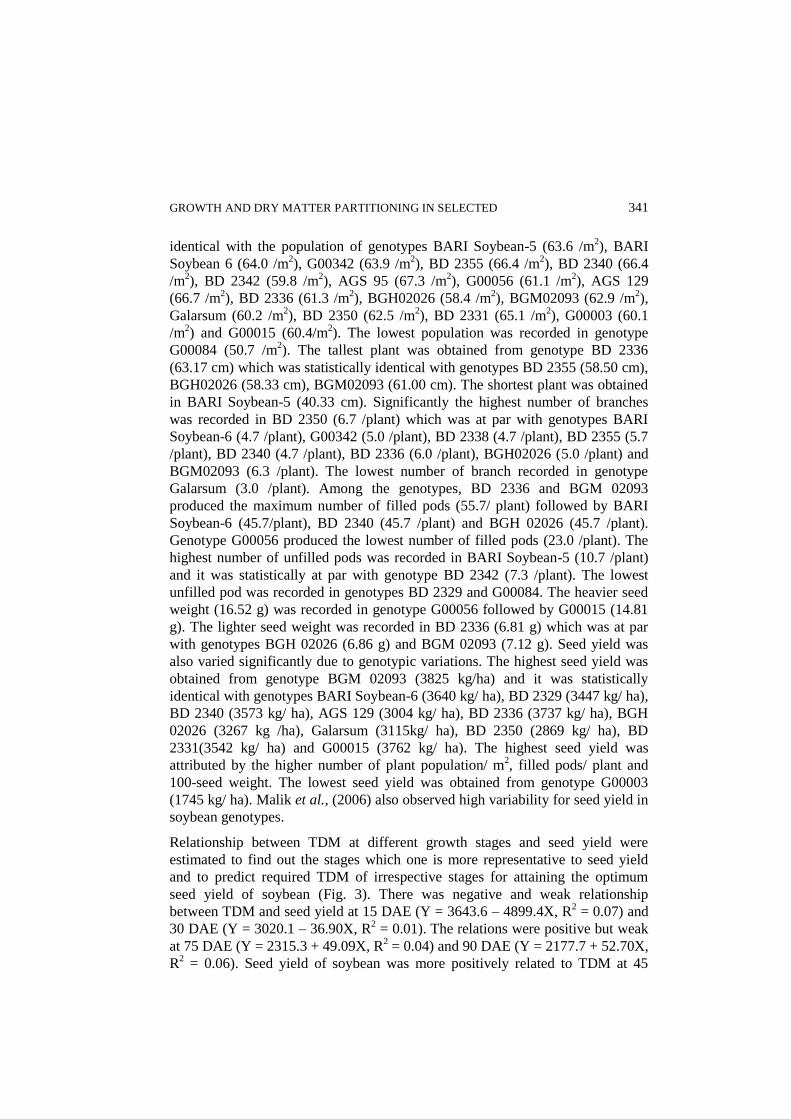
Total dry matter and their distribution in percent
Total dry matter and their distribution (%) of the plant of the respective soybean
genotypes at 90 DAE is presented in Table 3. The genotypes varied according to
their dry matter distribution (%) in different plant parts. Though the genotypes
BARI Soybean-6, G00342, BD 2338, BD 2340, BD 2331, G00003 and G00015
produced maximum dry matter, BARI Soybean-6 distributed 21.66% in stem,
4.83% in petiole, 9.24% in leaf blade and 64.27% in pods; G00342 distributed
19.04% in stem, 2.86% in petiole, 10.29% in leaf blade and 67.81% in pods; BD
2338 distributed 17.27% in stem, 6.57% in petiole, 22.01% in leaf blade and

338 KHAN et al.
54.06% in pods; BD 2334 distributed 15.56% in stem, 5.34% in petiole, 14.75%
in leaf blade and 64.35% in pods; BD 2331 distributed 20.915 in stem, 4.14% in
petiole, 11.84% in leaf blade and 63.11% in pods; G00003 distributed 21.50% in
stem, 6.9% in petiole, 18.75% in leaf blade and 52.85% in pods; G00015
distributed 16.21% in stem, 7.03% in petiole, 21.54% in leaf blade and 55.22% in
pods. Among the genotypes, G00056 distributed the highest dry matter in pods
(69.50%) with lowest in petiole (1.99%) and leaf blade (5.25%). Varietal
differences in dry matter accumulation with their partitioning in mustard are in
agreement with Khan et al., (2006).
Table 2. Total dry matter production of soybean genotypes at different days after
emergence (DAE).
Genotype Total dry matter (g/plant)
15 DAE 30 DAE 45 DAE 60 DAE 75 DAE 90 DAE
BARI Soybean-5 0.10 0.53 2.30 4.66 14.89 15.20
BARI Soybean-6 0.13 0.67 3.56 7.37 18.21 18.43
G00342 0.18 0.86 3.46 6.37 17.87 18.28
BD 2338 0.07 0.58 2.40 6.49 18.14 18.22
BD 2355 0.17 0.79 3.21 6.21 11.58 15.02
BD 2329 0.10 0.61 3.27 6.62 11.86 15.21
BD 2340 0.13 0.89 4.03 7.19 12.27 16.34
BD 2342 0.10 0.72 3.18 6.57 9.38 12.56
AGS 95 0.13 0.66 2.91 5.88 11.41 13.23
G00056 0.18 0.85 4.10 7.95 13.73 14.52
AGS 129 0.13 0.72 3.93 7.61 13.58 13.77
BD 2336 0.12 0.64 4.05 7.75 14.23 14.72
BGH02026 0.10 0.59 4.05 7.81 12.61 13.34
BGM02093 0.11 0.76 4.30 8.48 13.67 14.12
Galarsum 0.12 0.68 3.90 8.31 11.84 12.25
BD 2350 0.17 0.76 3.77 7.16 12.01 13.12
G00084 0.17 1.45 4.01 6.87 12.45 13.69
BD 2331 0.13 0.79 4.06 8.08 14.48 16.12
G00003 0.17 0.53 2.80 6.65 13.64 16.57
G00015 0.16 0.60 4.31 8.88 18.32 24.71
SE (±) 0.01 0.04 0.14 0.23 0.57 0.64
Mean 0.13 0.73 3.58 7.15 13.81 15.47
GROWTH AND DRY MATTER PARTITIONING IN SELECTED 339
Table 3. Total dry matter and their distribution in different plant parts at 90 days
after emergence of soybean genotypes.
Genotypes Stem
(%)
Petiole
(%)
Leaf blade
(%)
Pods
(%)
TDM
(g/plant)
BARI Soybean-5 18.15 4.71 15.98 61.15 15.20
BARI Soybean-6 21.66 4.83 9.24 64.27 18.43
G00342 19.04 2.86 10.29 67.81 18.28
BD 2338 17.27 6.57 22.10 54.06 18.22
BD 2355 20.04 7.72 27.10 45.13 15.02
BD 2329 17.89 3.83 11.15 67.13 15.21
BD 2340 15.56 5.34 14.75 64.35 16.34
BD 2342 24.65 2.65 6.45 66.25 12.56
AGS 95 18.27 4.76 17.34 59.63 13.23
G00056 23.26 1.99 5.25 69.50 14.52
AGS 129 22.71 4.22 14.36 58.71 13.77
BD 2336 22.55 4.84 13.43 59.18 14.72
BGH02026 26.83 3.11 7.81 62.25 13.34
BGM02093 24.70 2.55 6.19 66.56 14.12
Galarsum 23.80 4.42 15.47 56.31 12.25
BD 2350 17.87 4.87 19.88 57.39 13.12
G00084 25.03 6.02 18.75 50.20 13.69
BD 2331 20.91 4.14 11.84 63.11 16.12
G00003 21.50 6.90 18.75 52.85 16.57
G00015 16.21 7.03 21.54 55.22 24.71
SE(±) 0.73 0.36 1.33 1.44 0.64
Mean 20.90 4.67 14.38 60.05 15.47
Crop growth rate (CGR)
Crop growth rate of the soybean genotypes varied appreciably over the time (Fig.
2). At early stages, CGR was very slow till 30 DAE and thereafter increased
rapidly and the differences among the soybean genotypes persisted throughout
the growth period. Regardless of genotypes, CGR reached peak at 75 DAE and
thereafter declined in all genotypes. Maximum utilization of environmental
resources reached the plant at maximum CGR at the reproductive phase. After 75
DAE natural senescence of leaves might have tended to decline in CGR. At 45
DAE, CGR was maximum in genotype G00015 (16.51 g/m2/day) which was at
par in BGM02093 (15.74 g/m2/day) and followed by the growth rate of

340 KHAN et al.
genotypes BD 2336 (15.17 g/m2/day), BD 2326 (15.36 g/m
2/day) and BD
2331(14.57 g/m2/day). At 75 DAE it reached the highest in genotype BD 2338
(51.78 g/m2/day) which was at par with genotypes G00342 (51.11 g/m
2/day) and
BARI Soybean-6 (48.19 g/m2/day). At 90 DAE, the maximum CGR was
recorded in genotype G00015 (28.40 g/m2/day) followed by genotypes BD 2340
(18.10 g/m2/day), BD 2355 (15.27 g/m
2/day), BD 2329 (14.89 g/m
2/day) and BD
2342 (14.13 g/m2/day) genotypes.
0
10
20
30
40
50
60
15 30 45 60 75 90
Days after emergence
CG
R (
g m
-2d
ay
-1)
BARI soy 5 BARI soy-6 G00342 BD 2338
0
10
20
30
15 30 45 60 75 90
Days after emergence
CG
R (
g m
-2d
ay
-1)
BD 2355 BD 2329 BD 2340 BD 2342
0
10
20
30
40
50
15 30 45 60 75 90
Days after emergence
CG
R (
g m
-2d
ay
-1)
AGS 95 G00056 AGS 129 BD 2336
0
10
20
30
15 30 45 60 75 90
Days after emergence
CG
R (
g m
-2d
ay
-1)
BGH02026 BGM02093 Galarsum BD 2350
0
10
20
30
40
50
15 30 45 60 75 90
Days after emergence
CG
R (
g m
-2d
ay
-1)
G00084 BD 2331 G00003 G00015
Fig. 2. Crop growth rate (CGR) of soybean genotypes at different growth stages.
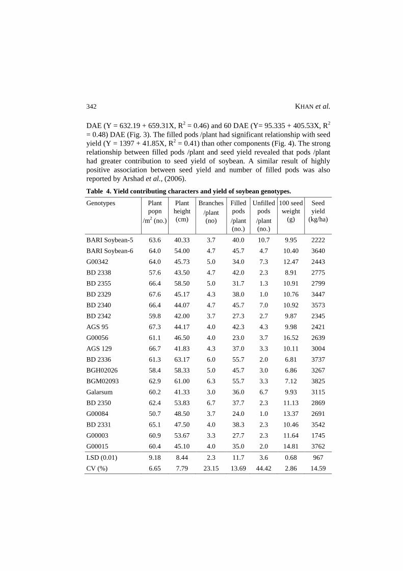
Yield and yield attributes
Plant population /m2, plant height, number of branches per plant, filled pods per
plant, unfilled pods per plant, 100-seed weight and seed yield of soybean showed
significant variations across the genotypes (Table 4). The maximum plant
population was obtained in genotype BD 2329 (67.6 /m2) and it was statistically
GROWTH AND DRY MATTER PARTITIONING IN SELECTED 341
identical with the population of genotypes BARI Soybean-5 (63.6 /m2), BARI
Soybean 6 (64.0 /m2), G00342 (63.9 /m
2), BD 2355 (66.4 /m
2), BD 2340 (66.4
/m2), BD 2342 (59.8 /m
2), AGS 95 (67.3 /m
2), G00056 (61.1 /m
2), AGS 129
(66.7 /m2), BD 2336 (61.3 /m
2), BGH02026 (58.4 /m
2), BGM02093 (62.9 /m
2),
Galarsum (60.2 /m2), BD 2350 (62.5 /m
2), BD 2331 (65.1 /m
2), G00003 (60.1
/m2) and G00015 (60.4/m
2). The lowest population was recorded in genotype
G00084 (50.7 /m2). The tallest plant was obtained from genotype BD 2336
(63.17 cm) which was statistically identical with genotypes BD 2355 (58.50 cm),
BGH02026 (58.33 cm), BGM02093 (61.00 cm). The shortest plant was obtained
in BARI Soybean-5 (40.33 cm). Significantly the highest number of branches
was recorded in BD 2350 (6.7 /plant) which was at par with genotypes BARI
Soybean-6 (4.7 /plant), G00342 (5.0 /plant), BD 2338 (4.7 /plant), BD 2355 (5.7
/plant), BD 2340 (4.7 /plant), BD 2336 (6.0 /plant), BGH02026 (5.0 /plant) and
BGM02093 (6.3 /plant). The lowest number of branch recorded in genotype
Galarsum (3.0 /plant). Among the genotypes, BD 2336 and BGM 02093
produced the maximum number of filled pods (55.7/ plant) followed by BARI
Soybean-6 (45.7/plant), BD 2340 (45.7 /plant) and BGH 02026 (45.7 /plant).
Genotype G00056 produced the lowest number of filled pods (23.0 /plant). The
highest number of unfilled pods was recorded in BARI Soybean-5 (10.7 /plant)
and it was statistically at par with genotype BD 2342 (7.3 /plant). The lowest
unfilled pod was recorded in genotypes BD 2329 and G00084. The heavier seed
weight (16.52 g) was recorded in genotype G00056 followed by G00015 (14.81
g). The lighter seed weight was recorded in BD 2336 (6.81 g) which was at par
with genotypes BGH 02026 (6.86 g) and BGM 02093 (7.12 g). Seed yield was
also varied significantly due to genotypic variations. The highest seed yield was
obtained from genotype BGM 02093 (3825 kg/ha) and it was statistically
identical with genotypes BARI Soybean-6 (3640 kg/ ha), BD 2329 (3447 kg/ ha),
BD 2340 (3573 kg/ ha), AGS 129 (3004 kg/ ha), BD 2336 (3737 kg/ ha), BGH
02026 (3267 kg /ha), Galarsum (3115kg/ ha), BD 2350 (2869 kg/ ha), BD
2331(3542 kg/ ha) and G00015 (3762 kg/ ha). The highest seed yield was
attributed by the higher number of plant population/ m2, filled pods/ plant and
100-seed weight. The lowest seed yield was obtained from genotype G00003
(1745 kg/ ha). Malik et al., (2006) also observed high variability for seed yield in
soybean genotypes.
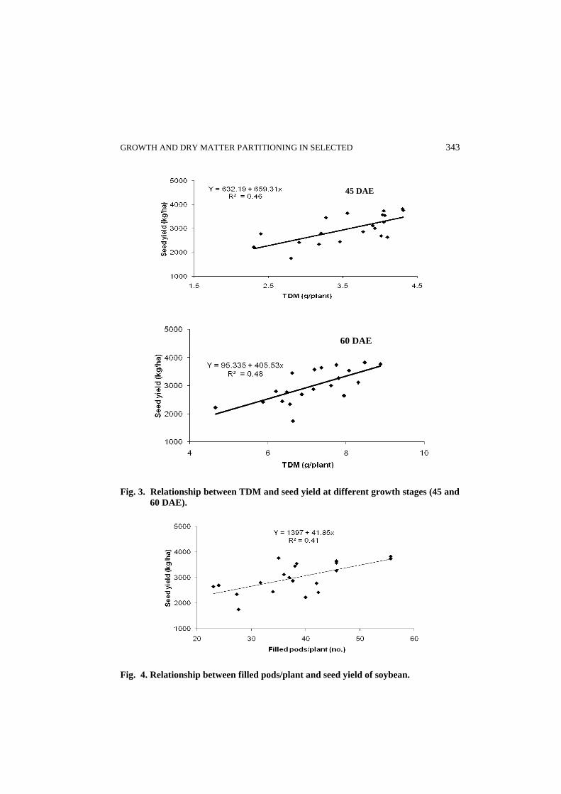
Relationship between TDM at different growth stages and seed yield were
estimated to find out the stages which one is more representative to seed yield
and to predict required TDM of irrespective stages for attaining the optimum
seed yield of soybean (Fig. 3). There was negative and weak relationship
between TDM and seed yield at 15 DAE (Y = 3643.6 – 4899.4X, R2 = 0.07) and
30 DAE (Y = 3020.1 – 36.90X, R2 = 0.01). The relations were positive but weak
at 75 DAE (Y = 2315.3 + 49.09X, R2 = 0.04) and 90 DAE (Y = 2177.7 + 52.70X,
R2 = 0.06). Seed yield of soybean was more positively related to TDM at 45
342 KHAN et al.
DAE (Y = 632.19 + 659.31X, R2 = 0.46) and 60 DAE (Y= 95.335 + 405.53X, R
2
= 0.48) DAE (Fig. 3). The filled pods /plant had significant relationship with seed
yield (Y = 1397 + 41.85X, R2 = 0.41) than other components (Fig. 4). The strong
relationship between filled pods /plant and seed yield revealed that pods /plant
had greater contribution to seed yield of soybean. A similar result of highly
positive association between seed yield and number of filled pods was also
reported by Arshad et al., (2006).
Table 4. Yield contributing characters and yield of soybean genotypes.
Genotypes Plant
popn
/m2 (no.)
Plant
height
(cm)
Branches
/plant
(no)
Filled
pods
/plant
(no.)
Unfilled
pods
/plant
(no.)
100 seed
weight
(g)
Seed
yield
(kg/ha)
BARI Soybean-5 63.6 40.33 3.7 40.0 10.7 9.95 2222
BARI Soybean-6 64.0 54.00 4.7 45.7 4.7 10.40 3640
G00342 64.0 45.73 5.0 34.0 7.3 12.47 2443
BD 2338 57.6 43.50 4.7 42.0 2.3 8.91 2775
BD 2355 66.4 58.50 5.0 31.7 1.3 10.91 2799
BD 2329 67.6 45.17 4.3 38.0 1.0 10.76 3447
BD 2340 66.4 44.07 4.7 45.7 7.0 10.92 3573
BD 2342 59.8 42.00 3.7 27.3 2.7 9.87 2345
AGS 95 67.3 44.17 4.0 42.3 4.3 9.98 2421
G00056 61.1 46.50 4.0 23.0 3.7 16.52 2639
AGS 129 66.7 41.83 4.3 37.0 3.3 10.11 3004
BD 2336 61.3 63.17 6.0 55.7 2.0 6.81 3737
BGH02026 58.4 58.33 5.0 45.7 3.0 6.86 3267
BGM02093 62.9 61.00 6.3 55.7 3.3 7.12 3825
Galarsum 60.2 41.33 3.0 36.0 6.7 9.93 3115
BD 2350 62.4 53.83 6.7 37.7 2.3 11.13 2869
G00084 50.7 48.50 3.7 24.0 1.0 13.37 2691
BD 2331 65.1 47.50 4.0 38.3 2.3 10.46 3542
G00003 60.9 53.67 3.3 27.7 2.3 11.64 1745
G00015 60.4 45.10 4.0 35.0 2.0 14.81 3762
LSD (0.01) 9.18 8.44 2.3 11.7 3.6 0.68 967
CV (%) 6.65 7.79 23.15 13.69 44.42 2.86 14.59
GROWTH AND DRY MATTER PARTITIONING IN SELECTED 343
Fig. 3. Relationship between TDM and seed yield at different growth stages (45 and
60 DAE).
Fig. 4. Relationship between filled pods/plant and seed yield of soybean.
45 DAE
60 DAE

344 KHAN et al.
Conclusion
Plant height, leaf area index, dry matter distribution in different parts, crop
growth rate and seed yield showed variation among the genotypes. The
genotypes BGM 02093, BD 2329, BD 2340, BD 2336, Galarsum, BD 2331 and
G00015 performed better in respect of higher accumulation of total dry matter
and seed yield. The selected genotypes should further be incorporated in breeding
trials to develop high yielding soybean varieties.
References
Aduloju, M.O., J. Mahamood and Y.A. Abayomi. 2009. Evaluation of soybean (Glycine
max (L) Merrill) genotypes for adaptability to a southern Guinea savanna
environment with and without P fertilizer application in north central Nigeria.
Afr. J. Agric. Res. 4: 556-563.
Arshad, M., N. Ali and A. Ghafoor. 2006. Character correlation and path coefficient in
soybean Glycine max (L.) Merrill. Pak. J. Bot. 38(1): 121-130.
FRG, 2005. Fertilizer Recommendation Guide. Bangladesh Agricultural Research
Council (BARC), Farmgate, Dhaka-1215.
Board, J.E., and B.G. Harville. 1992. Explanations for greater light interception in
narrow-vs. wide-row soybean. Crop Sci. 32: 198-202.
Ghatge, R.D., and R.N. Kadu. 1993. Genetic variability and heritability studies in
soybean. Advances in Plant Science 6: 224-228.
Hossain, M.A., and M.S.A. Khan. 2003. Genotypic variation in root growth, dry matter
accumulation, nutrient uptake and yield of Brassica species. Bangladesh J. Agril.
Sci. 30(1): 143-150.
Hossain, M.A., R.R. Saha and M.S.A. Khan. 2004. Root development, nutrient uptake
and yield performance of soybean as influenced by phosphorus fertilization.
Bangladesh J. Agril. Sci. 31(2): 161-168.
Khan, M.S.A., M.A. Hossain, M.N. Islam, M.S. Aktar and M.A. Rahman. 2006. Root
length density, dry matter accumulation and yield performance of mustard varieties
under rainfed condition. The Agriculturists 4(1&2): 141-148.
Khan, M.S.A. 2013. Evaluation of soybean genotypes in relation to yield performance,
salinity and drought tolerance. Ph.D. Dissertation. Dept. Agronomy, BSMRAU,
Salna, Gazipur.
Malik, M.F.A., A.S. Qureshi, M. Ashraf and A. Ghafoor. 2006. Genetic variability of the
main yield related characters in soybean. Int. J. Agri. Biol. 8(6): 815-819.
Messina, M. 1997. Soyfoods: Their role in disease prevention and treatment. In Liu, K.
(ed). Soybeans: Chemistry, Technology and Utilization, Chapman and Hall, New
York. Pp.442-466.

GROWTH AND DRY MATTER PARTITIONING IN SELECTED 345
Mondal, M.R.I., and M.A. Wahhab. 2001. Production Technology of Oilcrops. ORC,
BARI, Joydebpur, Gazipur. Pp.57-67
Radford, P.J. 1967. Growth analysis formulae – their use and abuse. Crop science. Vol.
7: 171-175.
Rasaily, S.K., N.D. Desai and M.U. Kukadia. 1986. Genetic variability in soybean
(Glycine max (L) Merrill). Gujrat Agric. University Res. J. 11: 57-60.
Yaklich, R.W., B. Vinyard, M. Camp and S. Douglass. 2002. Analysis of seed protein
and oil from soybean northern and southern region uniform tests. Crop Sci. 42:
1504-15.

346 KHAN et al.
ISSN 0258-7122
Bangladesh J. Agril. Res. 40(3): 347-361, September 2015
FARMERS LAND TENURE ARRANGEMENTS AND TECHNICAL
EFFICIENCY OF GROWING CROPS IN SOME SELECTED UPAZILAS
OF BANGLADESH
ISLAM M. A.1 AND MAHARJAN K. L.
2
Abstract
There are different land tenure arrangements in crop cultivation in Bangladesh.
It is needed to detect how farmers could maximize the benefits from proper
utilization of their resources and technologies in these prevailing different land
tenure arrangements in crop cultivation. The main quest of this study is to
analyze the actual production level and how much is deviated from maximum
attainable production level in terms of technical efficiencybased on average
gross revenue of output ha-1 in the cultivated various types of crops among
different categories of farmers and identifies the impact of the factors associated
with technical efficiency.In search of this research question a case study was
conducted in two Upazilas (Sub districts) in Bangladesh based on cross section
data. This data were collected from January to March, 2013. Age of the
household head, education, farm size, off-farm income and other concerned
issues were assessed. Maximum likelihood estimation and ordinary least square
regression techniques were used to estimate the parameters of the stochastic
production frontier.Ordinary least square regression was used to identify the
factors associated with technical efficiency. The study reveals that the technical
efficiency varied among different categories of farmers. But land rent (0.0575)
and weed management (0.0838) had significant positive impact on technical
efficiency. This detects the potentiality to improve the technical efficiency by
taking proper measures in land tenure arrangements in consideration of land rent
andprovide required weed management support for the farmers.
Keywords: Stochastic frontier approach, Maximum likelihood estimation,
ordinary least square regression method, land tenure, agricultural
production.
Introduction
Bangladesh is an agricultural developing country. The total area of Bangladesh is
144,000 sq. km, population is 150 million having cultivable area of 8.44 million
hectare (ha), the contribution of agriculture sector in the share of gross domestic
product is 23.50%, and this sector ensures 52% of the total employment of the
1Senior Assistant Secretary (OSD), Ministry of Public Administration, Bangladesh
Secretariat, Dhaka, Bangladesh, Presently, Ph.D Student, Graduate School for
International Development and Cooperation, Hiroshima University 1-5-1 Kagamiyama,
Higashi-Hiroshima, 739-8529 Japan, 2Professor, Graduate School for International
Development and Cooperation, Hiroshima University 1-5-1 Kagamiyama, Higashi-
Hiroshima, 739-8529 Japan.
348 ISLAM AND MAHARJAN
country(BBS, 2011).The major cultivated cereal crops in Bangladesh areHYV
Boro, T. Aman and B. Aman. The average yield of these crops are 3.90, 2.26 and
1.90 Ton ha-1 (BBS, 2011).The following three farming categories are observed
in the country based on share cropping, fixed rent and mortgaging tenancy
arrangements:(a) Owner farming (b) Owner cum tenant farming(c) Tenant
farming.
Farming category in the study areas
In Bangladesh, the percentages of owner, owner cum tenant and tenant farmers
are 65%, 22% and 13% respectively( BBS , 2011).Where as these percentages of
owner, owner cum tenant and tenant farmers in the study areas are 44.5%, 33.5%
and 22% respectively (DAE, 2013).
Owner farmers cultivate owned land and mortgaged land in owner farming. In
cultivating this owned land, owner farmers get the whole amount of the produced
crop as net revenue after deducting the production cost. In the case of mortgaged
land, cultivators need not to pay any share of the produced output to the land
owner but need to pay a certain amount of mortgaged money and duration of this
mortgaged land persist until the mortgaged money can be repaid by
themortgagor(who mortgaged out the land).
Owner cum tenant farmers cultivate owned land, mortgaged land, fixed
rentedland and share cropped land. In cultivation of this fixed rented land, a fixed
amount of money is needed to payannually to the land owners by the
cultivators(who rented in the land in fixed renting system).The terms and
conditions of mortgaged land in owner cum tenant farming are as same as
mortgaged land in owner farming. In most cases, share cropping system of
cultivation has been found inefficient in terms of low resource use, low
productivity and deprivation from land lords.ThereforeBangladesh government
passed the land reform ordinance 1984 in order to protect the interest of tenant or
share croppers from landlords as well as to increase crop productivity at farm
level through efficient use of resources.
According to this land reform ordinance of Bangladesh, tenant will provide labor,
land will be provided by the land owner and rest other input costs will be shared
between the land owner and tenant farmers in 50:50 ratio, and the produced
output will be shared based on the same ratio between the land owner and tenant
farmers to get proper incentive in agricultural production(LRB, 1982). But in
practice, output sharing is conducted according tothis legal provision but input
costs sharing is not practiced properly(Ullah, 1996). Again,this crop sharing
arrangement is applied in case of share cropped land of the owner cum tenant
farmers also.

FARMERS LAND TENURE ARRANGEMENTS AND TECHNICAL EFFICIENCY 349
Measuring technical efficiency is one of theapproachesfor understanding how
farmers could maximize the benefits from the proper utilization of existing
resources and technologies.This approach can be conducted using production,
cost or profit function. The first approach is called technical efficiency(Battese
and Coelli,1995).
The adaptation of proper variety and other socioeconomic factors had significant
impact on technical efficiency (TE) in rice production of different farming
system in Bangladesh,Barmon (2013)found that farmers producing modern
variety of rice were more technically efficient than farmers producing rice in
prawn gher(Area used for prawn cultivation) farming in the coastal region of
Bangladesh.
The mean technical efficiency of Nepalese rice seed growers was 81% and it was
found that there was a wide variation in technical efficiency due to education
level and experience of the farmers in seed production (Khanal and Maharjan,
2013). The mean technical efficiency of rice cultivation in Bangladesh was 69%,
indicating that there is a scope of 31% improvement in technical efficiency and
availability of credit was found significant positive impact on technical efficiency
(Ahmed, 2011). There are variations in the level of technical efficiency in
agriculture within the sub- sectors of crop, livestock and fish cultivation. It is
revealed that credit had a significant positive impact on the technical efficiency
of all of these sub-sectors (Ahmed, 2010). The noted literatures clearly
demonstrate that the stochastic frontier approach is widely used in agricultural
economics studies. In case of Bangladesh, it was observed that fragmentation of
land generates production inefficiency in agriculture sector (Wadud, 2003).In this
study it was also found that farmers could increase their rice production by 9 to
39% if they could operate at full technical efficiency level with their existing
resources and technology.
The pattern of land ownership affects gross revenue per hectare by affecting the
efficient use of inputs. Considering the tenancy status of farm lands in
Bangladesh, 58% of the land is operated by owner, 40% by owner cum tenant,
and 2% by tenant farmers (Tenaw, et al., 2009).
There are studies (Ahmed, 2012; Asadullah, 2005) about land tenure and tenancy
system in Bangladesh refuting the claim about the significance of land leasing in
and consequence enhancements in viability of small farms. It is cited evidence
that the terms of tenancy in Bangladesh were very oppressive. In large portion of
the cases the land owner exacted 50% of the produced crops as rent without
sharing any parts of the cost and at least 5% of the cases the share of rent was
more than 50%. Thus, when full cost accounting is applied the share croppers
incurred a negative return (Ullah, 1996). The effect of land fragmentation on
China’s agriculture was examined by Wan and Cheng (2001) and found that a
350 ISLAM AND MAHARJAN
new land tenure institution emphasizing consolidation significantly improves the
production efficiency. The mean technical efficiency of Nigerian agriculture was
77%; it means that there is a scope of 23% improvement in technical efficiency
(Idiong, 2007).
The productivity of agricultural production may varyamong different categories
of farming due to discriminate use of various production inputs and managerial
factors in Bangladesh, which needs proper evaluation through econometric
model.There are some studies about various aspects of agricultural production in
Bangladesh including technical efficiency based on different socioeconomic
issues,but an updated study is needed on technical efficiency based on land
tenure aspect to trace out the proper policy implication for the agricultural
development in Bangladesh.Therefore, the present study was conducted with the
following specific objectives.
Objectives of the study
o To analyze the technical efficiency of different categories of farmers in
cultivating various cultivated crops in a cropping year to detect the actual
production level and deviated from the maximum attainable production
level of the farmers;
o To identify the impact of the factors influencing technical efficiency of
different categories of farmers;
o To recommendfor betterment of agricultural production;
Materials and Method
(a) Description of the Study location and sampling technique
adopted:This study was carried out at Basailupazila ofTangail district and
TitasupazilaofComilla district in Bangladesh. The area of Basailupazila was
158 sq.km, and population was 76,002.The area of Titasupazila was 107.19
sq.km, and population was 183,425.These two Upazilas were selected as
farmers of these twoUpazilas were getting proper agricultural support of the
government due to location advantage, which can represent the overall
farming characteristics of the country.The purposive stratified sampling
technique was followed as the share of owner, owner cum tenant and tenant
farmers were very disproportionate in the study areas(DAE, 2013).
(b) Method of data collection and period of study:Three hundred
respondents were taken equally one hundred for each category and fifty
respondents from each upazila.Data were collected in survey methodfrom
January, 2013 - March, 2013 to trace out the proper factors oftechnical
efficiency under different land tenure arrangements based on the cultivated
FARMERS LAND TENURE ARRANGEMENTS AND TECHNICAL EFFICIENCY 351
crops in a cropping year. The major cultivated crops in the study areas were
HYV Boro, T. Aman and B. Aman. Mustard, jute, wheat or pulses were
cultivated as minor crops. Normally two or three crops were cultivated in
each plot of land among these crops in a year.
(c) Analytical technique adopted: The collected data were analyzed by
using STATA9.Stochastic frontier model was used to measure the technical
efficiency of the different categories of farmers based on their average gross
revenue of output ha-1in the cultivated various types of land.This study
considers the stochastic frontier approach with the assumption that the actual
production cannotexceed the maximum possible production with the given
input quantities and it is suggested to determine the factors responsible for
inefficiency (Aigner et al.,1977 and Meeusen and van den Broeck,1977).
It was used in a two stage procedure. In the first stage,TE was computed and in
the second stage socioeconomic variables of farm households were
regressedagainst this TE using ordinary least square(OLS) regression method to
identify their impact.Since the value of TE is 0<TE<1,it justifies using OLS
technique(Kalirajan,1999;Piya,Kiminami and Yagi,2012).The stochastic frontier
model used in this study as follows:
𝐿𝑛Yi β0 β𝐿𝑛𝑥𝑖 + 𝑣𝑖 − 𝑢𝑖… (1)
Where, logarithm Yi is theaverage gross revenue of output ha-1in different types
of cultivated land, βis the vector of parameters to be estimated,xi presents inputs.
These inputs includes per hectare averagecost of labor, power tiller, chemical
fertilizer andirrigation in various categories of cultivated land of the different
tenure groups of farmers. Land rent was taken as a proxy indicator of surplus as
ownership patterns as well as cultivated land categories were different among
owner,owner cum tenant and tenant farmers. This land rent was taken at the rate
of the cost of mortgaged land of the owner farmers based on their cultivated
mortgaged land, but for the owner cum tenant and tenant farmers this land rent
was taken at the rate of cost of cultivated share cropped land of the owner cum
tenant and tenant farmers in the study areas.
It was found in the study areas that if half of the seed cost was provided to the
tenant by the land owner then land owner claimed half of the produced by-
product, and even sometimes without sharing this seed cost the half of the
produced by- product was claimed also based on customary rule. To avoid this
complexity, the price of by-product was not taken into account in estimating
gross revenue as well as seed was not included due to this reason.vi presents the
error term accounting for random variation in gross revenue due to factors
outside the control of farmers.
352 ISLAM AND MAHARJAN
Another error term ui presents error associated with farm level inefficiency and
this is assumed to have 0 mean with variance (𝜎u2)and distributed half
normally. Similarly,vi is assumed to have zero mean and constant variance(𝜎v2)
and distributed normally with independent with each ui. Both of these error terms
are supposed to be uncorrelated with explanatory variables xi.
The loglikelihood function for half normal model is given in equation (2).This
likelihood function estimates whether the variation among the observation is due
to inefficiency. From the likelihood function we get 𝜎2 and ℷ2.
Where, ℷ2 = 𝜎𝑢2 + 𝜎𝑣2 andℷ2 = 𝜎𝑢2/𝜎2 . If =0, it indicates there is no
inefficiency effect and the variation in the data is due to random noise only.The
higher the valueofℷ the more will be inefficiency effects explained by the model.
𝐿𝑛 𝐿 𝑌𝑖 𝛽, 𝜎ℷ = −1
2𝐿𝑛 𝜋𝜎2 + 𝐿𝑛∅{
𝑛
𝑖=1
−ℇ𝑖ℷ
𝜎}-
1
2𝜎2 ℇ𝑖2𝑛
𝑖=1 … (2)
Where, Yi is the vector log ofaverage gross revenue of output ha-1 in different
types of cultivated landℇ𝑖=vi-ui=Ln Yi-xi 𝛽 is the composite error and∅(𝑥𝑖) is a
cumulative distribution functionof the standard normal variable evaluated at xi.
Empirical model:
Empirical model for production
lnYi= a+b1lnX1 + b2 lnX2+ b3 lnX3 + b4 ln X4 +Ui
Where,
Y= Average gross revenue of output (Takaha-1) of different types of
cultivated land in different types of farming
a, b1, b2, b3, b4= Parameters to be estimated
X1=Average cost of labor (Taka ha-1)in different types of cultivated land
X2= Average cost of power tiller (Taka ha-1)in different types of cultivated
land
X3= Average cost of chemical fertilizer (Taka ha-1)in different types of
cultivated land
X4= Average cost of irrigation (Taka ha-1)in different types of cultivated land
Ui= Error term
Empirical model for TE
The TE of the farmers in the context of stochastic frontier model can be
expressed as:
TEi =𝑌𝑖
𝑌∗= 𝑓 𝑥𝑖; 𝛽 exp(𝑣𝑖 − 𝑢𝑖)/𝑓 𝑥𝑖; 𝛽 𝑒𝑥𝑝(𝑣𝑖) = 𝑒𝑥𝑝 −𝑢𝑖 … (3)

FARMERS LAND TENURE ARRANGEMENTS AND TECHNICAL EFFICIENCY 353
Where, 𝑌 ∗ is the maximum possible average gross revenue of output ha-1 in
different types of cultivated land,Yi,xi, 𝛽, 𝑣𝑖, 𝑇𝐸𝑖and uiare as explained
earlier.TEi measures the average gross revenue of output ha-1 in different types
of cultivated land of the farmers relative to the maximum possible average gross
revenue ofoutput ha-1 in different types of cultivated land that can be produced
using the same cost of input vectors. This value of TEi is 0 to 1.
If TEi=1,Yi achieves the maximum value of 𝑓 𝑥𝑖; 𝛽 𝑒𝑥𝑝 𝑣𝑖 .IfTEi is less than
1,thatindicates the shortfall of gross revenue of output from the maximum
possible level.Thissituation is characterized by stochastic elements,which vary
among the farmers.The following equation (4) was used to identify the impact of
socioeconomic variables on TE.
𝑇𝐸𝑖 = δ0+𝛿𝐿𝑛𝑍𝑖 + 𝜔𝑖 …(4)
Where, presents the parameters associated with socioeconomic
variables(zi),and𝜔𝑖 is the error term.
The variables for the study were chosen considering both production theory and
local context of the farmers.Analysis of variance (ANOVA) was used to analyze
the mean difference of technical efficiency of the farmers.
Regression analysis was used to identify the impact of the factors associated
with technical efficiency.In using this stochastic frontier model Wald chi2 test
showed significant result(P= 0.0000), that indicates the fitness of the model. All
of these stochastic frontier model, ANOVA and regression analyses were used
based on overall study areas.For the regression analysis OLS method was used,
because OLS is easier to analyze mathematically than many other regression
technique. It produces solution those are easily interpretable; OLS is the best
unbiased linear estimator of the model coefficient.
Moreover, robust regression technique of this OLS model mitigates the problem
of data variation. Before running this OLS model data were validated using
Variance Inflation Factor(VIF) and robust regression method for
multicollinearity and heteroskedasticity.
This OLS model was used in the many other similar studies including the study
conducted by Ahmed (2012),on Agricultural Land Tenancy. This OLS model
was also used in the study on Farm Productivity and efficiency in Rural
Bangladesh: The role of Education Revisited(Asadullah,2005).
Results and Discussion
(1) Socioeconomic characteristics of respondent farmers
Table 1 presents the socioeconomic characteristics of the respondent farmers.
The average year of education of head of the household (HHH1) were 4.65, 3.96

354 ISLAM AND MAHARJAN
and 2.22 in owner, owner cum tenant and tenant farmers respectively. This year
of education varied from 0 to 14 years, from 0 to 10 years, and from 0 to 5 years
in owner, owner cum tenant and tenant farmers respectively.
The average farm size of owner, owner cum tenant and tenant farmers were 0.77,
0.74 and 0.70 ha respectively.This farm size varied in owner, owner cum tenant
and tenant farmers from 0.23 to 4.08 ha, from 0.23 to 2.27 ha and from 0.23 to
2.72 ha respectively.
The mean land rents were BDT 18,010, 9,730 and 16,050 ha-1
among owner,
owner cum tenant and tenant farmers respectively.This land rent varied from
BDT 8,000 to 83,803, from BDT 5,000 to 39,696 and from BDT 3,000 to75,000,
ha-1
respectively.
The percentages of adoption of new crop adopting farmers were 100, 100 and 87
among owner, owner cum tenant and tenant farmers respectively. But this
percentage was 96 in overall.
The percentages of weed management adopting farmers were 100, 98 and 5
amongowner, owner cum tenant and tenant farmers, but this percentage was 68 in
overall.
From the discussion of socioeconomic characteristics of the farmers, it is
concluded that tenant farmers were in most dis-advantageous position in farming
among these different tenure categories of farmers in consideration of farm size
and all other socioeconomic aspects.
(2) Study variables
Table 2.1presentsthe mean and standard deviation of the study variables.The
mean gross revenues of owner, owner cum tenant and tenant farmers were BDT
94,558, 93,941 and103,916ha-1
respectively.
Those varied from BDT15,845 to 234,650, BDT 25,641 to 395,200 and BDT
11,115 to 185,250
ha-1
inowner, owner cum tenant and tenant farmers respectively.The mean labor
costs of owner, owner cum tenant and tenant farmers were BDT7,133,4,438 and
10,938ha-1
respectively. These labor cost varied in the range of BDT 2,205 to
16,540, BDT 2,205 to 11,026and BDT1,500 to 16,540 among owner, owner cum
tenant and tenant farmers respectively.The mean power tiller costswere BDT
2,419,1,626 and 4,084 ha-1
in owner, owner cum tenant and tenant farmers
respectively.
This power tiller cost varied from BDT 1,470 to 4,410, BDT1,143 to 4,410and
BDT1,700to 4,940 ha-1
in owner, owner cum tenant and tenant farmers
respectively.

FARMERS LAND TENURE ARRANGEMENTS AND TECHNICAL EFFICIENCY 355
Ta
ble
1.
So
cio
eco
no
mic
ch
ara
cter
isti
c o
f th
e sa
mp
le h
ou
seh
old
s.
Va
ria
ble
s O
wn
er f
arm
ers
Ow
ner
cu
m t
ena
nt
farm
ers
Ten
an
t fa
rm
ers
Ov
era
ll
Age
of
HH
H1(y
ear)
Ed
uca
tio
n (
yea
r)
Occ
up
atio
n o
f H
HH
1 (
1)
(%)
Fam
ily l
abo
r(L
FU
2)
Far
m s
ize(
ha)
Off
far
m i
nco
me
( T
aka)
Land
ren
t
Exte
nsi
on (
1)
(%)
Sav
ing (
1)
(%)
Cre
dit
(1
) (%
)
% o
f ad
op
tio
n o
f new
cro
p
Wee
d m
anag
em
ent
(1)
(%)
Liv
esto
ck n
it(L
SU
3)
51
.43(9
.98
)
4.6
5(3
.5)
42
3.6
5(0
.83
)
0.9
0(0
.67
)
69
,640
(76
,94
4)
18
,010
(18
,39
7)
98
98
77
10
0
10
0
3.0
6(1
.21
)
50
.51(8
.99
)
3.9
4(2
.79
)
76
3.5
4(0
.77
)
0.8
0(0
.33
)
28
,750
(44
,01
6)
9,7
30(6
,58
9)
60
46
36
10
0
98
3.0
0(0
.73
)
43
.77(9
.69
)
2.2
2(1
.97
)
72
3.1
3(0
.89
)
0.7
05(0
.52
)
26
,020
(18
,95
8)
16
,050
(13
,70
6)
4
2
20
87
5
2.3
2(0
.91
)
48
.57(9
.56
)
3.6
1(1
.75
)
63
3.4
4(0
.82
)
0.8
0(0
.50
)
41
,469
(46
,63
9)
14
,596
(14
,18
3)
54
49
44
96
68
2.7
9(0
.95
)
So
urc
e: F
ield
surv
ey (
20
13
) N
ote
: F
igure
s in
the
par
enth
eses
ind
icat
e S
tand
ard
Dev
iati
on.
356 ISLAM AND MAHARJAN
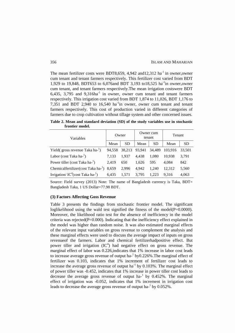
The mean fertilizer costs were BDT8,659, 4,942 and12,312 ha-1
in owner,owner
cum tenant and tenant farmers respectively. This fertilizer cost varied from BDT
1,929 to 19,848, BDT653 to 6,076and BDT 3,193 to18,525 ha-1
in owner,owner
cum tenant, and tenant farmers respectively.The mean irrigation costswere BDT
6,435, 3,795 and 9,316ha-1
in owner, owner cum tenant and tenant farmers
respectively. This irrigation cost varied from BDT 1,874 to 11,026, BDT 1,176 to
7,351 and BDT 2,940 to 16,540 ha-1
in owner, owner cum tenant and tenant
farmers respectively. This cost of production varied in different categories of
farmers due to crop cultivation without tillage system and other concerned issues.
Table 2. Mean and standard deviation (SD) of the study variables use in stochastic
frontier model.
Variables Owner
Owner cum
tenant Tenant
Mean SD Mean SD Mean SD
Yield( gross revenue Taka ha-1) 94,558 38,213 93,941 34,489 103,916 33,501
Labor (cost Taka ha-1) 7,133 1,937 4,438 1,080 10,938 3,791
Power tiller (cost Taka ha-1) 2,419 650 1,626 595 4,084 842
Chemicalfertilizer(cost Taka ha-1) 8,659 2,996 4,942 1,240 12,312 5,560
Irrigation/ IC4(cost Taka ha-
1) 6,435 1,571 3,795 1,223 9,316 4,063
Source: Field survey (2013) Note: The name of Bangladesh currency is Taka, BDT=
Bangladesh Taka, 1 US Dollar=77.98 BDT.
(3) Factors Affecting Goss Revenue
Table 3 presents the findings from stochastic frontier model. The significant
loglikelihood using the wald test signified the fitness of the model(P=0.0000).
Moreover, the likelihood ratio test for the absence of inefficiency in the model
criteria was rejected(P=0.000). Indicating that the inefficiency effect explained in
the model was higher than random noise. It was also estimated marginal effects
of the relevant input variables on gross revenue to complement the analysis and
these marginal effects were used to discuss the average impact of inputs on gross
revenueof the farmers. Labor and chemical fertilizerhadpositive effect. But
power tiller and irrigation (IC4) had negative effect on gross revenue. The
marginal effect of labor was 0.226,indicates that 1% increase in labor cost leads
to increase average gross revenue of output ha-1 by0.226%.The marginal effect of
fertilizer was 0.103, indicates that 1% increment of fertilizer cost leads to
increase the average gross revenue of output ha-1
by 0.103%. The marginal effect
of power tiller was -0.452, indicates that 1% increase in power tiller cost leads to
decrease the average gross revenue of output ha-1 by 0.452%. The marginal
effect of irrigation was -0.052, indicates that 1% increment in irrigation cost
leads to decrease the average gross revenue of output ha-1 by 0.052%.

FARMERS LAND TENURE ARRANGEMENTS AND TECHNICAL EFFICIENCY 357
Table 3. Maximum likelihood estimates and marginal effect.
Variables Coefficients P value Marginal effects
Labor
Power tiller
Chemical fertilizer
Irrigation(IC4)
Constant
0.306(0.000021)
-0.690(0.000014)
0.138(0.000019)
-0.072(0.000021)
14.36(0.00011)
0.000***
0.000***
0.000***
0.000***
0.000***
0.226
-0.452
0.103
-0.052
Loglikelihood:-298.05***σ2= 1.71ℷ =7.77 likelihood ratio= 2.7*** N= 300, *** indicates
significant at 1% level of significance.
(4) Farm specific technical efficiency of the farmers
Tables (4.1, 4.2) present frequency distribution and mean difference of technical
efficiency among owner, owner cum tenant and tenant farmers. From the tables it
is found that there was a variation among the number of farmers as well as
significant mean difference of technical efficiencyamong owner, owner cum
tenant and tenant farmers.
Table 4.1 Frequency distribution of farm specifictechnical efficiency of the
farmers.
Rage of TE Owner(%) Owner cum
tenant(%) Tenant(%)
< 0.50 29 70 50
0.51- 0.60 28 12 28
0.61- 0.70 18 06 09
0.71- 0.80 06 08 03
0.80+ 19 04 10
Table 4.2 Farm specific technical efficiency of the farmers.
Farming category Technical efficiency P value
Owner 0.603(0.211) 0.0000***
Owner cum tenant 0.444(0.184)
Tenant 0.527(0.192)
Note: Number of observation: 300 ***Significant at 1% level of significance, figures in
the parentheses indicate Std. Dev.
The result shows that there was 60% mean technical efficiency of owner farmers that varied from 7.9% to 99.9%. Indicates that owner farmers could improve technical efficiency by 40%.This mean technical efficiency in owner cum tenant farmers was 44% that varied from 3.8% to 99.9%, indicates that owner cum
tenant farmers could improve technical efficiency by 56%. Again average technical efficiency of tenant farmers was 52.7% in the range of 5.8% to 99.9%, which indicates that tenant farmers could improve technical efficiency by 47.3%.

358 ISLAM AND MAHARJAN
(5) Factors affecting technical efficiency of the farmers
Table 5 presents the summary result of the impact of socioeconomic
variables.We tested fourteen socio economic explanatory variables against
technical efficiency in OLS regression. From the analysis, it was found that the
direction of the response of the variables land rent andweed management were as
per the hypothesis and these variables hadsignificant positive impact on technical
efficiency.Indicate that1% increment of land rent leads to increase TE by
5.75%.This might be for the better incentive of land rent as a surplus in farming.
Proper use of weed management leads to increase TE by 0.0838%. This might be
better utility of weed management in farming.Education, farm status, farm size
and adoption of new crop were significant but did not show expected sign.
Table 5. Measurement unit, expected sign and parameter estimates of the OLS model.
Variables Measurement unit Expected
sign Coefficients P value
Age of the HHH1 Year + 0.0015(.001) 0.264
Education Year of formal education + -0.0128(.004) 0.003***
Occupation 1= primary, 0= secondary
(dummy)
+ -0.0146(.030) 0.634
Farm status (Owner
cum tenant)
2= owner cum tenant
+ -0.0797(.032) 0.015**
Farm status( Tenant) 3= tenant + 0.0431(.059) 0.467
Family labor(LFU2) LFU
2 + 0.0110(.015) 0.466
Ln farm size Hectare + -0.0857(.023) 0.000***
Ln off- farm income BDT + -0.0212(.016) 0.198
Ln land rent BDT + 0.0575(.019) 0.003***
Extension services 1 = Yes, 0= No (dummy) + 0.0452(.035) 0.208
Saving 1 = Yes, 0= No (dummy) + 0.0392(.037) 0.296
Credit 1 = Yes, 0= No (dummy) + 0.0386(.032) 0.233
Adaptation of new
crop
1 = Yes, 0= No (dummy) + -0.1202(.061) 0.053*
Weed management 1 = Yes, 0= No (dummy) + 0.0838(.039) 0.034**
Livestock unit
(dummy)
LSU3 + -0.0205(.015) 0.196
Cons BDT + 0.1812(.261) 0.488
Note: Farm status:1= owner, 2= owner cum tenant, 3= tenant (dummy) Number of
observation: 300 R-squared = 28 Root MSE= 0.176 Figures in the parentheses indicate
Std. Err. ***, ** and * Significant at 1%, 5% and 10% level of significance respectively.

FARMERS LAND TENURE ARRANGEMENTS AND TECHNICAL EFFICIENCY 359
In case of education, this might be the provided education was not properly
oriented in farming. For the case of farm status of owner cum tenant farmers, this
might be due to extensive use of owned land of owner cum tenant farmers. For
farm size, this might be due to extensive use of owned land of the owner farmers
as well as owner cum tenant farmers. In the case ofadoption of new crop, this
might be the existing cultivation of crop is economically more viable than
adoption of new crop based on the socioeconomic context of the farmers.Other
variables did not show significant impact on technical efficiency.
Conclusion and recommendation
In this study technical efficiency of different categories of farmers was estimated
using stochastic frontier model and analyzed the estimated technical efficiency
using ANOVA.It was found that there was a statistically significant difference
from zero in the level of technical efficiency among owner, owner cum tenant
and tenant farmers.It was alsofound significantly positive influence of landrent
and weed management on technical efficiency.
From the discussions it can be discerned that, there is a potentiality for the
enhancement of technical efficiency in ensuring change by taking measures in
land tenure arrangements in proper implementation of the land reform ordinance
1984 that will ascertain higher surplus for the share croppersin share cropped
land and provide weed management support for the farmers.Those might lead to
attain higher technical efficiency. This study recommends the government to take
necessary measures on that direction.
End Note:
(1) HHH stands for household head.
(2) Labor force unit(LFU) is the measurement of family labor where people
from 15-59 years regardless of sex were categorised 1 person=1 LFU, but
in the case of children 10-14 and elderly people more than 59 years old 1
person= 0.5 LFU.
(3) Livestock unit(LSU) is the aggregate of different types of livestock kept at
household standard unit calculated using following equivalents;
1 adult buffalo = 1 LSU,1 immature buffalo= 0.5 LSU 1 cow= 0.8 LSU,
1sheep or goat= 0.2 LSU and 1 poultry or pigeon=0.1 LSU (Khanal and
Maharjan,2013).
(4) IC stands for irrigation cost. This irrigation cost is paid in kind as one
fourth of the total produced crop.

360 ISLAM AND MAHARJAN
References
Ahmed, S. 2012. Agricultural Land Tenancy in Rural Bangladesh: Productivity Impact
and Process of Contract Choice.
Ahmed, M. S. 2010. Technical Efficiency of Agricultural Farms in Khulna, Bangladesh:
Stochastic Frontier Approach.
Asadullah, N. M. 2005. Farm Productivity and Efficiency in Rural Bangladesh: The Role
of Education Revisited SKOPE, Department of Economics Uiversity of Oxford, UK.
Bangladesh Bureauof Statistics (BBS). 2011. Year Book of Agricultural Statistics of
Bangladesh Bureau of Statistics, Ministry of Planning, Government of the people`s
republic of Bangladesh, Dhaka.
Barmon, B.K. 2013. Technical Efficiency and Total Factor Productivity of Modern
Variety Paddy Production UnderDifferent Farming System in Bangladesh,
Asia Pacific Journal of Rural Development 1: 58-78.
Bamatraf, A. R. 2000.Impact of Land Tenure and other Socioeconomic Factors on
Mountain Terrace Maintenance in Yemen, International Food Policy Research
Institute, Washington D.C, USA.
Bilkis, R. 2012. Trend in Productivity Research in Bangladesh Agriculture: A Review of
Selected Articles, Asian Business Review, volume 1.
Battese, G. E., and Coelli, T. J. 1995. A model for Technical Inefficiency Effect in a
Stochastic Frontier Production Function for Panel Data, Empirical Economics,
20(1995): 325-332.
Department of Agricultural Extension (DAE). 2013. Department of Agriculture
Extension, Tangail and Comilla districts, Bangladesh.
Hossain, M. 1991.Agriculture in Bangladesh: Performance Problems and Prospects
University press limited.
Idiong, I. C. 2007.Estimation of Farm Level Technical Efficiency in Small Scale Swamp
Rice Production inCross River State of Nigeria: A Stochastic Frontier Approach,
World Journal of Agricultural Sciences, (5):653-658.
Kalirajan, K. P. 1999. The Importance of Effective and Efficient Use in the Adoption of
Technologies:A Micro Panel Data Analysis Journal of Production Analysis Pp. 113-
126.
Khanal, N. P., and Maharjan, K. L. 2013. Technical Efficiency of Rice Seed Growers in
the Tarai region of Nepal, Journal of rural problems, 49(1):27-31.
Land Reform Board (LRB).1982. Land Reform Report of Land Reform Committee, Land
Reform Board, Ministry of Land, Government of the People`s Republic of
Bangladesh, Dhaka.
Meeusen, W. and Van den Broeck, J. 1977.Efficiency Estimation from Cobb Douglas
Production Function with Composed Error. International Economic Review, 18(2):
435-444.
FARMERS LAND TENURE ARRANGEMENTS AND TECHNICAL EFFICIENCY 361
S. Piya. A. Kiminami and Yagi, H. 2012. Comparing the Technical Efficiency of Rice
Farmers in Urban and Rural Areas: A Case Study from Nepal, Trends in Agriculture
Economics, Pp. 48-60.
Tenaw, S., Islam, Z. K. M., Parviainen, T. 2009. Effects of Land Tenure and Property
Rights on Agricultural Productivity in Ethiopia, Namibia and Bangladesh University
of Helsinki, Department of Economics and Management, Helsinki, Finland.
Ullah, M. 1996. Land Livelihood and Change in Rural Bangladesh, University press
limited.
Wadud, M. A. 2003. Technical, Allocative and Economic Efficiency in Bangladesh: A
Stochastic and DEA approach, The Journal of Developing Areas, 37(1):109-126.

362 ISLAM AND MAHARJAN

ISSN 0258-7122
Bangladesh J. Agril. Res. 40(3): 363-379, September 2015
FACTORS AFFECTING THE ADOPTION OF IMPROVED VARIETIES
OF MUSTARD CULTIVATION IN SOME SELECTED SITES OF
BANGLADESH
M. A. MONAYEM MIAH1, SADIA AFROZ
2
M. A. RASHID3 AND S. A. M. SHIBLEE
4
Abstract
Mustard is a leading oil crop in Bangladesh. Relevant data and information on
the adoption of improved mustard varieties is very scanty and sporadic in
Bangladesh. Therefore, an attempt was made to assess the extent of adoption of
improved mustard varieties and their management practices at farm level. The
study used data from 540 mustard growing farmers under Manikgonj, Rajshahi
and Dinajpur districts. Probit regression model along with other descriptive
statistics were used to analyze the collected data. Analysis revealed that the farm
level adoption of different production practices were not encouraging as most
farmers did not follow the recommendations made by Bangladesh Agricultural
Research Institute (BARI) for mustard cultivation. The variety adoption scenario
was also discouraging since only 40% of the farmers cultivated improved
mustard varieties. However, farmers showed positive attitude towards adoption
of improved mustard varieties since about 53% of the adopters wanted to
increase area under improve mustard cultivation in next growing season
considering the high yielding ability, low cultivation cost, high profit, and less
labour requirements. Although mustard is considered to be a profitable crop,
many farmers showed negative attitude towards its production due to some
drawbacks. Non-availability of improved mustard seed was also found to be a
barrier to its adoption at farm level.
Keywords: Improved mustard, variety adoption, farmers’ attitude, production
practices.
Introduction
Rapeseed and mustard are popularly called ‘Mustard’ which is a leading oilseed
crop, covering about 80% of the total oilseed area and contributing to more than
60% of the total oilseed production in Bangladesh. It is a cold loving crop which
is grown during Rabi season.
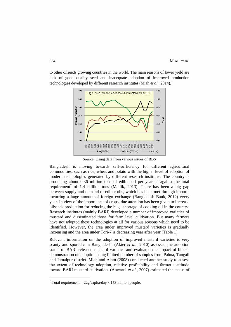
The total area and production of mustard is 276.11 thousand hectare and 262.00
thousand tons (Fig 1). The present mustard yield (0.95 t/ha) is very low as compared
1Senior Scientific Officer,
3&4Principal Scientific Officer. Agricultural Economics
Division, Bangladesh Agricultural Research Institute (BARI), Joydebpur, Gazipur-1701, 2Assistant Chief, Ministry of Planning, Sher-e-Bangla Nagar, Dhaka-1207, Bangladesh.
364 MIAH et al.
to other oilseeds growing countries in the world. The main reasons of lower yield are
lack of good quality seed and inadequate adoption of improved production
technologies developed by different research institutes (Miah et al., 2014).
Source: Using data from various issues of BBS
Bangladesh is moving towards self-sufficiency for different agricultural
commodities, such as rice, wheat and potato with the higher level of adoption of
modern technologies generated by different research institutes. The country is
producing about 0.36 million tons of edible oil per year as against the total
requirement* of 1.4 million tons (Mallik, 2013). There has been a big gap
between supply and demand of edible oils, which has been met through imports
incurring a huge amount of foreign exchange (Bangladesh Bank, 2012) every
year. In view of the importance of crops, due attention has been given to increase
oilseeds production for reducing the huge shortage of cooking oil in the country.
Research institutes (mainly BARI) developed a number of improved varieties of
mustard and disseminated those for farm level cultivation. But many farmers
have not adopted these technologies at all for various reasons which need to be
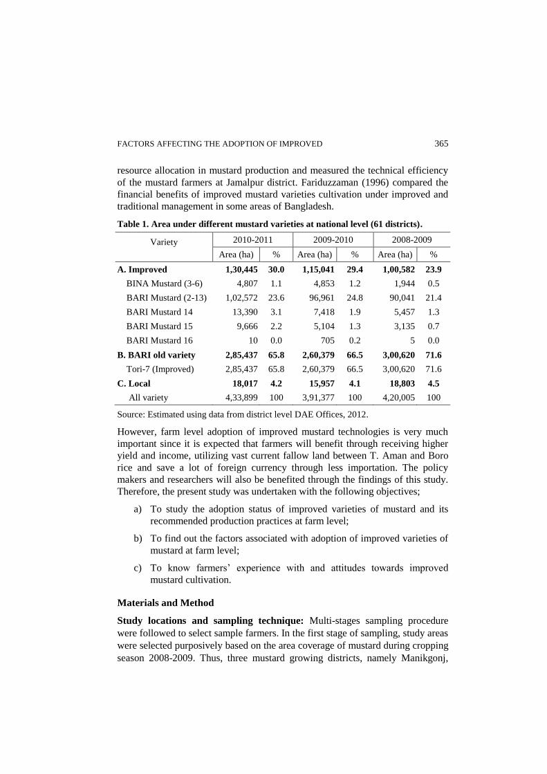
identified. However, the area under improved mustard varieties is gradually
increasing and the area under Tori-7 is decreasing year after year (Table 1).
Relevant information on the adoption of improved mustard varieties is very
scanty and sporadic in Bangladesh. (Akter et al., 2010) assessed the adoption
status of BARI released mustard varieties and evaluated the impact of blocks
demonstration on adoption using limited number of samples from Pabna, Tangail
and Jamalpur district. Miah and Alam (2008) conducted another study to assess
the extent of technology adoption, relative profitability and farmer’s attitude
toward BARI mustard cultivation. (Anwarul et al., 2007) estimated the status of
* Total requirement = 22g/capita/day x 153 million people.
FACTORS AFFECTING THE ADOPTION OF IMPROVED 365
resource allocation in mustard production and measured the technical efficiency
of the mustard farmers at Jamalpur district. Fariduzzaman (1996) compared the
financial benefits of improved mustard varieties cultivation under improved and
traditional management in some areas of Bangladesh.
Table 1. Area under different mustard varieties at national level (61 districts).
Variety
2010-2011 2009-2010 2008-2009
Area (ha) % Area (ha) % Area (ha) %
A. Improved 1,30,445 30.0 1,15,041 29.4 1,00,582 23.9
BINA Mustard (3-6) 4,807 1.1 4,853 1.2 1,944 0.5
BARI Mustard (2-13) 1,02,572 23.6 96,961 24.8 90,041 21.4
BARI Mustard 14 13,390 3.1 7,418 1.9 5,457 1.3
BARI Mustard 15 9,666 2.2 5,104 1.3 3,135 0.7
BARI Mustard 16 10 0.0 705 0.2 5 0.0
B. BARI old variety 2,85,437 65.8 2,60,379 66.5 3,00,620 71.6
Tori-7 (Improved) 2,85,437 65.8 2,60,379 66.5 3,00,620 71.6
C. Local 18,017 4.2 15,957 4.1 18,803 4.5
All variety 4,33,899 100 3,91,377 100 4,20,005 100
Source: Estimated using data from district level DAE Offices, 2012.
However, farm level adoption of improved mustard technologies is very much
important since it is expected that farmers will benefit through receiving higher
yield and income, utilizing vast current fallow land between T. Aman and Boro
rice and save a lot of foreign currency through less importation. The policy
makers and researchers will also be benefited through the findings of this study.
Therefore, the present study was undertaken with the following objectives;
a) To study the adoption status of improved varieties of mustard and its
recommended production practices at farm level;
b) To find out the factors associated with adoption of improved varieties of
mustard at farm level;
c) To know farmers’ experience with and attitudes towards improved
mustard cultivation.
Materials and Method
Study locations and sampling technique: Multi-stages sampling procedure
were followed to select sample farmers. In the first stage of sampling, study areas
were selected purposively based on the area coverage of mustard during cropping
season 2008-2009. Thus, three mustard growing districts, namely Manikgonj,
366 MIAH et al.
Rajshahi, and Dinajpur consisting high (covered ≤10% of total mustard area),
medium (≤5 to >10% area), and low (>5% area) mustard growing areas were
selected for the study. In the second stage, in all nine Upazilas under three
selected districts were purposively selected taking three Upazila from each
district. Before selecting Upazilas, data on the area and production of mustard
were collected from Upazila DAE offices and the highest three mustard growing
Upazilas were selected for the study. Thirdly, three agricultural blocks were also
purposively selected in consultation with Agricultural Officer of the respective
Upazila. Finally, a total of 540 mustard growing households (3 districts ×
3Upazilas × 3 Blocks × 20 HHs) were randomly selected from a complete list of
mustard growing farmers.
Method of data collection and period of study: Data and relevant information
were collected through personal interview with sampled farmers using a pre-
tested structured interview schedule. The researchers and trained enumerators
collected data and information for this study. Data and information were
collected during the period from October 2011 to October 2012.
Analytical techniques: For assessing the level of adoption of crop management
technologies, respondent farmers were grouped into three categories such as
high, medium, and low adopter based on the percent of farmers followed
recommended practice with respect to each technology. A higher percentage
indicates a higher level of adoption, while a lower percentage indicates a lower
level of adoption of a technology. Adoption level was categorized as (70-100%)
as high, (50-69%) as medium, and <50% as low. This category of adoption was
followed by different authors (Islam et al., 2013; Salam et al., 2011; Miah et al.,
2010; Akter et al., 2010) in the past.
Probit and Logit models have been used extensively by agricultural production
and farming systems economists for studying and analyzing farmers’ adoption
and diffusion of agricultural interventions. In Pakistan, Malik et al., (1991) and
Heisey et al., (1990) used Probit model to examine the role of credit in
agricultural development and to identify the determinants of adoption of wheat
varieties. Traxler and Byerlee (1992) also used this analysis to identify the
characteristics of insecticide farmers. In the present study, Probit regression
model was used to find out the factors of adoption and non-adoption of improved
varieties of mustard. In order to ascertain the probability of adoption of improved
mustard varieties, the following empirical Probit model was employed. Since the
dependent variable is dichotomous, Ordinary Least Square (OLS) method is not
suitable. Therefore, MLE method was followed to run the Probit model using
STATA software. The empirical probit model was as follows:
Ai = α + βiXi + ……..+ Ui

FACTORS AFFECTING THE ADOPTION OF IMPROVED 367
Where,
Ai = Farmers adopting improved mustard variety (If adopted = 1; Otherwise
= 0), α = Intercept, Xi = Explanatory variables, βi = Coefficients of respective
variables, and Ui = Error term
The adoption of improved mustard variety is likely to be influenced by different
explanatory variables. The variables are X1 = Farm size (in decimal), X2 = Family
labour (in No./ha), X3 = Training received on oilseed (in No.), X4 = Availability
of improved seed (score), X5 = Influence of neighbouring farmers (score), X6 =
Influence of SAAO (score), X7 = Cosmopolitness of the farmer (score), and X8 =
Extension contact of the farmers (score).
The procedures of measuring qualitative variables included in the model are
briefly discussed below.
Influence of neighbouring farmers and SAAO: These variables were measured
based on the level of influences of neighbouring farmers and SAAO in adopting
improved mustard variety. Zero value was assigned for ‘no influence’ and 4 for
‘strong influence’. Therefore, the possible scores of these variables ranged from
0 to 4.
Availability of improved seed: The availability of improved mustard seeds was
assigned different values ranging from 0 to 4 (0 = not available, 4 = plenty) and
these values were considered as score.
Cosmopolitness: Different values (0 for no visit and 3 for frequent visit) were
assigned, based on frequency, for different places of visit. The actual score was
then calculated by adding all the values. Possible scores ranged from 0 to 9.
Extension contact: Ten different extension Medias were considered in this
study. All these Medias were assigned different values (0 for no contact and 4 for
regular contact) according to their importance. The actual score was measured by
adding all the values. The possible scores for extension contact were ranged from
0 to 40.
Results and Discussion
Adoption of mustard varieties in the study locations
The farm level adoption of mustard varieties mostly depended on the
dissemination process of BARI in association with the Department of
Agricultural Extension (DAE). So far BARI has developed and disseminated 16
improved rapeseed and mustard varieties to the farmers. Adoption of mustard
varieties at household levels has been discussed below.

368 MIAH et al.
Household level adoption revealed that about 40.2% mustard farmers adopted
improved varieties and almost 60% adopted BARI old variety (Tori-7). The
national level data on mustard area also revealed that Tori-7 is the dominant
variety across the country which covered 68.15% mustard area (Table 1). Short
duration and to some extent tolerant to biotic and abiotic stresses are the main
characteristics that make Tori-7 popular to most of the farmers in the study areas.
Among improved varieties, BARI Mustard-15 and BARI Mustard-9 were the
highly adopted varieties in the study areas, but area covered by these two
varieties is very low at national level. However, BAU Sampod, BARI Mustard-9
and BARI Mustard-15 were the highly adopted varieties in Dinajpur, Rajshahi,
and Manikgonj district respectively (Table 2).
Table 2. Level of adoption of different mustard varieties in different study locations.
Variety % of farmers adopted the variety
Manikgonj Rajshahi Dinajpur All area
A. Improved 40.0 30.0 50.5 40.2
BARI Mustard-9 5.6 (10) 16.7 (30) 8.3 (15) 10.2 (55)
BARI Mustard-14 16.1 (29) 2.8 (5) 1.1 (2) 6.7 (36)
BARI Mustard-15 17.2 (31) 10.6 (19) 12.2 (22) 13.3 (72)
BARI Mustard-16 1.1 (2) -- -- 0.4 (2)
BAU Sampod -- -- 17.8 (32) 5.9 (32)
Indian Mustard -- -- 11.1 (20) 3.7 (20)
B. BARI old variety 60.0 70.0 49.5 59.8
Tori-7 60.0 (108) 70.0 (126) 49.5 (89) 59.8 (323)
All varieties 100 (180) 100 (180) 100 (180) 100 (540)
Note: Figures in the parentheses indicate the number of respondent farmers.
Source: Field survey, 2011-12.
The respondent farmers were found to be very much enthusiastic towards BARI
Mustard-14 and 15 due to their short life cycle (80-85 days) and high yielding
potentials. But the rate of adoption of these two varieties was not satisfactory in
the study areas mainly due to lack of knowledge about these varieties and non-
availability of seed. The same reasons of low adoption of improved rice varieties
were also stated in the study conducted by Jabber and Alam (1993). However,
the adoption rates of these two varieties may be higher in other mustard growing
areas. Experienced farmers and extension personnel opined that the availability
of seeds of short duration T. Aman rice (e.g. BINA Dhan-7), BARI Mustard-14,
and BARI Mustard-15 could bring revolution in mustard cultivation in
Bangladesh.
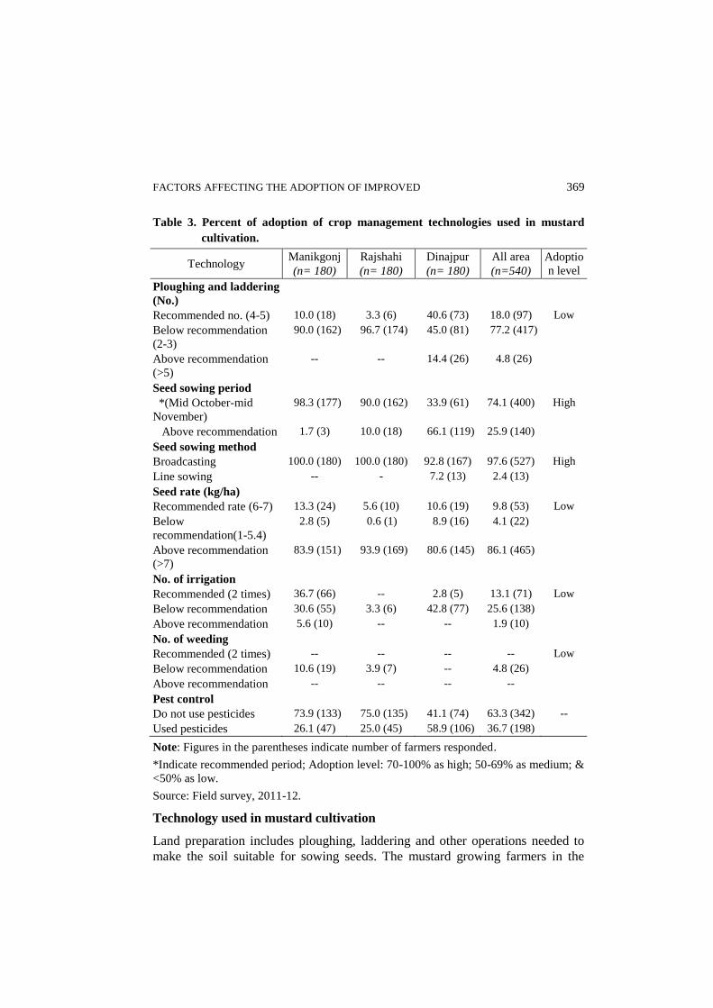
FACTORS AFFECTING THE ADOPTION OF IMPROVED 369
Table 3. Percent of adoption of crop management technologies used in mustard
cultivation.
Technology Manikgonj
(n= 180)
Rajshahi
(n= 180)
Dinajpur
(n= 180)
All area
(n=540)
Adoptio
n level
Ploughing and laddering
(No.)
Recommended no. (4-5) 10.0 (18) 3.3 (6) 40.6 (73) 18.0 (97) Low
Below recommendation
(2-3)
90.0 (162) 96.7 (174) 45.0 (81) 77.2 (417)
Above recommendation
(>5)
-- -- 14.4 (26) 4.8 (26)
Seed sowing period
*(Mid October-mid
November)
98.3 (177) 90.0 (162) 33.9 (61) 74.1 (400) High
Above recommendation 1.7 (3) 10.0 (18) 66.1 (119) 25.9 (140)
Seed sowing method
Broadcasting 100.0 (180) 100.0 (180) 92.8 (167) 97.6 (527) High
Line sowing -- - 7.2 (13) 2.4 (13)
Seed rate (kg/ha)
Recommended rate (6-7) 13.3 (24) 5.6 (10) 10.6 (19) 9.8 (53) Low
Below
recommendation(1-5.4)
2.8 (5) 0.6 (1) 8.9 (16) 4.1 (22)
Above recommendation
(>7)
83.9 (151) 93.9 (169) 80.6 (145) 86.1 (465)
No. of irrigation
Recommended (2 times) 36.7 (66) -- 2.8 (5) 13.1 (71) Low
Below recommendation 30.6 (55) 3.3 (6) 42.8 (77) 25.6 (138)
Above recommendation 5.6 (10) -- -- 1.9 (10)
No. of weeding
Recommended (2 times) -- -- -- -- Low
Below recommendation 10.6 (19) 3.9 (7) -- 4.8 (26)
Above recommendation -- -- -- --
Pest control
Do not use pesticides 73.9 (133) 75.0 (135) 41.1 (74) 63.3 (342) --
Used pesticides 26.1 (47) 25.0 (45) 58.9 (106) 36.7 (198)
Note: Figures in the parentheses indicate number of farmers responded.
*Indicate recommended period; Adoption level: 70-100% as high; 50-69% as medium; &
<50% as low.
Source: Field survey, 2011-12.
Technology used in mustard cultivation
Land preparation includes ploughing, laddering and other operations needed to
make the soil suitable for sowing seeds. The mustard growing farmers in the
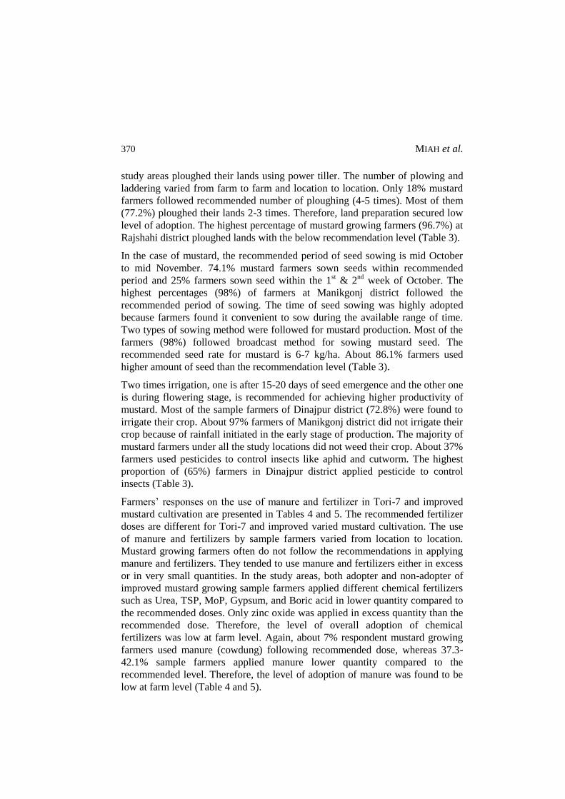
370 MIAH et al.
study areas ploughed their lands using power tiller. The number of plowing and
laddering varied from farm to farm and location to location. Only 18% mustard
farmers followed recommended number of ploughing (4-5 times). Most of them
(77.2%) ploughed their lands 2-3 times. Therefore, land preparation secured low
level of adoption. The highest percentage of mustard growing farmers (96.7%) at
Rajshahi district ploughed lands with the below recommendation level (Table 3).
In the case of mustard, the recommended period of seed sowing is mid October
to mid November. 74.1% mustard farmers sown seeds within recommended
period and 25% farmers sown seed within the 1st & 2
nd week of October. The
highest percentages (98%) of farmers at Manikgonj district followed the
recommended period of sowing. The time of seed sowing was highly adopted
because farmers found it convenient to sow during the available range of time.
Two types of sowing method were followed for mustard production. Most of the
farmers (98%) followed broadcast method for sowing mustard seed. The
recommended seed rate for mustard is 6-7 kg/ha. About 86.1% farmers used
higher amount of seed than the recommendation level (Table 3).
Two times irrigation, one is after 15-20 days of seed emergence and the other one
is during flowering stage, is recommended for achieving higher productivity of
mustard. Most of the sample farmers of Dinajpur district (72.8%) were found to
irrigate their crop. About 97% farmers of Manikgonj district did not irrigate their
crop because of rainfall initiated in the early stage of production. The majority of
mustard farmers under all the study locations did not weed their crop. About 37%
farmers used pesticides to control insects like aphid and cutworm. The highest
proportion of (65%) farmers in Dinajpur district applied pesticide to control
insects (Table 3).
Farmers’ responses on the use of manure and fertilizer in Tori-7 and improved
mustard cultivation are presented in Tables 4 and 5. The recommended fertilizer
doses are different for Tori-7 and improved varied mustard cultivation. The use
of manure and fertilizers by sample farmers varied from location to location.
Mustard growing farmers often do not follow the recommendations in applying
manure and fertilizers. They tended to use manure and fertilizers either in excess
or in very small quantities. In the study areas, both adopter and non-adopter of
improved mustard growing sample farmers applied different chemical fertilizers
such as Urea, TSP, MoP, Gypsum, and Boric acid in lower quantity compared to
the recommended doses. Only zinc oxide was applied in excess quantity than the
recommended dose. Therefore, the level of overall adoption of chemical
fertilizers was low at farm level. Again, about 7% respondent mustard growing
farmers used manure (cowdung) following recommended dose, whereas 37.3-
42.1% sample farmers applied manure lower quantity compared to the
recommended level. Therefore, the level of adoption of manure was found to be
low at farm level (Table 4 and 5).

FACTORS AFFECTING THE ADOPTION OF IMPROVED 371
Table 4. Farmers’ practice on using manure and fertilizer in improved
variety mustard cultivation.
Particular
% of farmers used manure and fertilizers Adoption
level Manikgonj
(n=72)
Rajshahi
(n=54)
Dinajpur
(n=91)
All area
(n=217)
Cowdung (ton/ha)
*8-10 ton/ha 13.2 (12) 1.4 (1) 3.7 (2) 6.9 (15) Low
Below recommendation 38.5 (35) 16.7 (12) 63.0(34) 37.3 (81)
Above recommendation 26.4 (24) -- -- 11.1 (24)
Urea (kg/ha)
*250-300 kg/ha 7.0 (5) -- 2.1 (2) 3.2 (7) Low
Below recommendation 86.1 (62) 98.1 (53) 90.1 (82) 91.7(199)
Above recommendation 7.0 (5) 1.8 (1) 5.4 (5) 5.1 (11)
TSP (kg/ha)
*170-180 kg/ha 4.2 (3) -- 1.1 (1) 1.8 (4) Low
Below recommendation 41.7 (30) 42.6 (23) 61.5 (56) 50.2(109)
Above recommendation 34.7 (25) 18.7 (17) 19.3 (42)
MoP (kg/ha)
*85-100 kg/ha 5.6 (4) 5.5 (3) 19.8 (18) 11.5 (25) Low
Below recommendation 37.5 (27) 66.7 (36) 40.7 (37) 46.5(101)
Above recommendation 12.5 (9) 9.3 (5) 54.9 (50) 29.5 (64)
Gypsum (kg/ha)
*150-180 kg/ha -- 5.6 (3) 4.3 (4) 2.8 (6) Low
Below recommendation 33.3 (24) 35.2 (19) 29.7 (27) 32.3 (70)
Above recommendation 6.9 (5) 3.7 (2) 8.8 (8) 6.9 (15)
Zinc (kg/ha)
*5-7 kg/ha 4.2 (3) 1.8 (1) 1.1 (1) 2.3 (5) Low
Below recommendation 1.4 (1) -- 5.4 (5) 2.8 (6)
Above recommendation 5.6 (4) 5.6 (3) 26.4 (24) 14.3 (31)
Boron (kg/ha)
*10-15 kg/ha 5.6 (4) 1.8 (1) 9.9 (9) 6.5 (14) Low
Below recommendation 8.3 (6) 9.3 (5) 16.4 (15) 12.0 (26)
Above recommendation 1.4 (1) 5.6 (3) 3.3 (3) 3.2 (7)
Note: Figures in the parentheses indicate number of farmers responded
*Recommended dose; Adoption level: 70-100% as high; 50-69% as medium; and <50%
as low.
Source: Field survey, 2011-12.
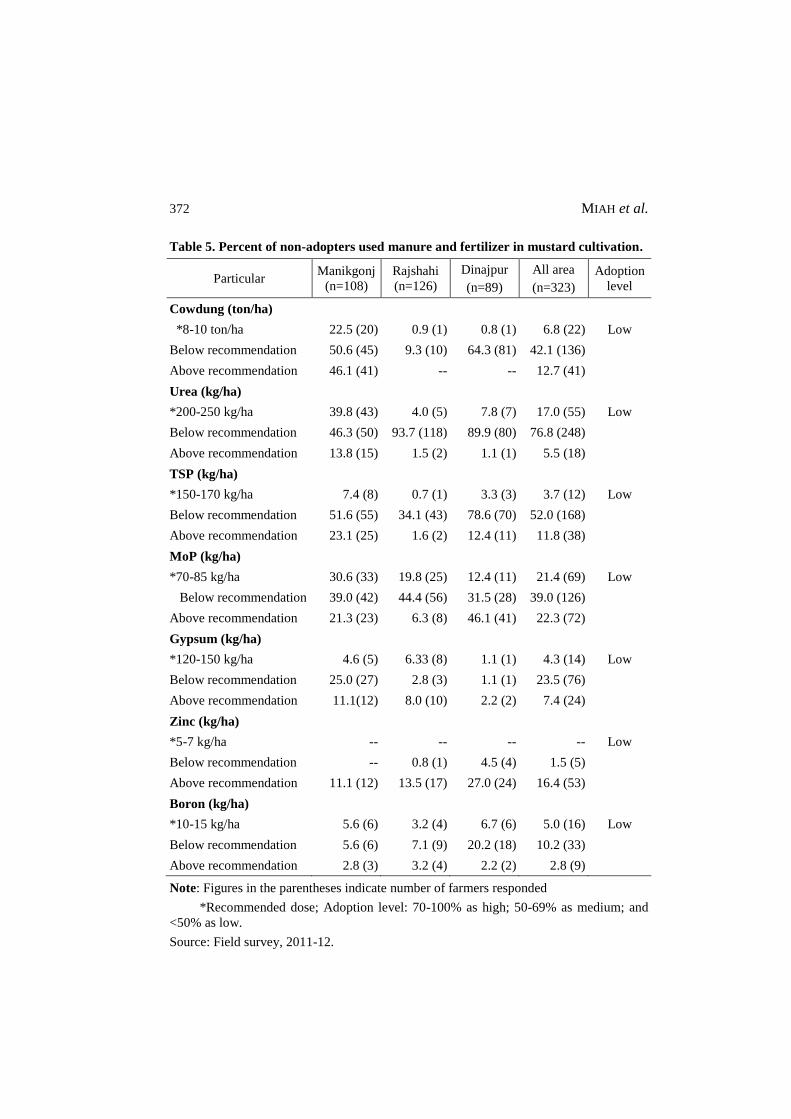
372 MIAH et al.
Table 5. Percent of non-adopters used manure and fertilizer in mustard cultivation.
Particular Manikgonj
(n=108)
Rajshahi
(n=126)
Dinajpur
(n=89)
All area
(n=323)
Adoption
level
Cowdung (ton/ha)
*8-10 ton/ha 22.5 (20) 0.9 (1) 0.8 (1) 6.8 (22) Low
Below recommendation 50.6 (45) 9.3 (10) 64.3 (81) 42.1 (136)
Above recommendation 46.1 (41) -- -- 12.7 (41)
Urea (kg/ha)
*200-250 kg/ha 39.8 (43) 4.0 (5) 7.8 (7) 17.0 (55) Low
Below recommendation 46.3 (50) 93.7 (118) 89.9 (80) 76.8 (248)
Above recommendation 13.8 (15) 1.5 (2) 1.1 (1) 5.5 (18)
TSP (kg/ha)
*150-170 kg/ha 7.4 (8) 0.7 (1) 3.3 (3) 3.7 (12) Low
Below recommendation 51.6 (55) 34.1 (43) 78.6 (70) 52.0 (168)
Above recommendation 23.1 (25) 1.6 (2) 12.4 (11) 11.8 (38)
MoP (kg/ha)
*70-85 kg/ha 30.6 (33) 19.8 (25) 12.4 (11) 21.4 (69) Low
Below recommendation 39.0 (42) 44.4 (56) 31.5 (28) 39.0 (126)
Above recommendation 21.3 (23) 6.3 (8) 46.1 (41) 22.3 (72)
Gypsum (kg/ha)
*120-150 kg/ha 4.6 (5) 6.33 (8) 1.1 (1) 4.3 (14) Low
Below recommendation 25.0 (27) 2.8 (3) 1.1 (1) 23.5 (76)
Above recommendation 11.1(12) 8.0 (10) 2.2 (2) 7.4 (24)
Zinc (kg/ha)
*5-7 kg/ha -- -- -- -- Low
Below recommendation -- 0.8 (1) 4.5 (4) 1.5 (5)
Above recommendation 11.1 (12) 13.5 (17) 27.0 (24) 16.4 (53)
Boron (kg/ha)
*10-15 kg/ha 5.6 (6) 3.2 (4) 6.7 (6) 5.0 (16) Low
Below recommendation 5.6 (6) 7.1 (9) 20.2 (18) 10.2 (33)
Above recommendation 2.8 (3) 3.2 (4) 2.2 (2) 2.8 (9)
Note: Figures in the parentheses indicate number of farmers responded
*Recommended dose; Adoption level: 70-100% as high; 50-69% as medium; and
<50% as low.
Source: Field survey, 2011-12.

FACTORS AFFECTING THE ADOPTION OF IMPROVED 373
Determinants of adoption of improved mustard varieties
The adoption of improved mustard varieties was likely to be influenced by
different socio-economic factors. Data in Table 6 show that farm size, family
labor, training on oilseed, influences of neighbor, influences of SAAO,
cosmopoliteness, and extension contact had positive and importantly influence on
the adoption of improved mustard varieties in the study areas.
Marginal coefficient indicate that if farm size increased by 100%, the probability
of adopting improved mustard varieties would increase at 0.017%. Again, if the
number of family labor increased by 100% the probability of adopting improved
mustard varieties would increase by 1.01%. The coefficients of seed availability,
influences of SAAO, cosmopolitness, and extension contact were positive and
significant. If these variables increase by 100% the probability of adopting
improved mustard varieties would increase by 13.26%, 14.67%, 5.06%, and
1.18% respectively (Table 7).
Table 6. Maximum likelihood estimates of variable determining adoption of
improved mustard varieties among respondent farmers.
Explanatory variable Coefficient Standard Error z-statistic Probability
Constant -
3.70295***
0.413278 -8.96 0.000
Farm size (decimal) 0.00045* 0.0002515 1.80 0.072
Family labour (number/ha) 0.02763*** 0.0045008 6.14 0.000
Training on oilseed (number) 0.09835 0.1206966 0.81 0.415
Availability of HYV seed
(score)
0.36302*** 0.0902197 4.02 0.000
Influences of neighbour
(score)
0.07377 0.0740819 1.00 0.319
Influences of SAAO (score) 0.40150*** 0.0699717 5.74 0.000
Farmers’ cosmopolitness
(score)
0.13839** 0.0607972 2.28 0.023
Extension contact (score) 0.03230** 0.0150383 2.15 0.032
Note: Number of observation = 537; LR chi-square (8) = 321.6; Log likelihood = -
190.47736;
‘***’ ‘**’ & ‘*’ represent significant at 1%, 5% and 10% level respectively
Higher score value represents the higher probability of improved variety adoption
Source: Field survey, 2011-12.

374 MIAH et al.
Table 7. Marginal effect of the variables determining adoption of improved mustard
varieties among respondent farmers.
Explanatory variable Dy/dx Standard
Error z-statistic Probability
Farm size (decimal) 0.000165* 0.00009 1.80 0.071
Family labour (number/ha) 0.010094*** 0.00167 6.04 0.000
Training on oilseed (number) 0.035930 0.04414 0.81 0.416
Availability of HYV seed (score) 0.132622*** 0.03307 4.01 0.000
Influences of neighbour (score) 0.026949 0.02699 1.00 0.318
Influences of SAAO (score) 0.146682*** 0.02669 5.50 0.000
Farmers’ cosmopolitness (score) 0.050557** 0.02218 2.28 0.023
Extension contact (score) 0.011799** 0.00551 2.14 0.032
Note: ‘***’ ‘**’ & ‘*’ represent significant at 1%, 5% and 10% level respectively
Farmers’ attitudes toward mustard cultivation
The respondent farmers were asked to mention the possibility of devoting more
area for improved mustard cultivation. In the case of adopters, almost 52% of the
mustard farmers showed their interest to increase mustard cultivation in the next
year. In the case of non-adopters, 46.65% farmers showed their interest to expand
mustard cultivation. About 48% adopter and 52% non-adopter indicated that they
would not increase mustard area in the next year. Although mustard is a
profitable crop, 50.19% farmers will not increase mustard cultivation in the next
year due to various reasons (Table 8).
Table 8. Farmers’ perceptions regarding further increase or decrease of area under
mustard cultivation in the next year,
Particulars % of farmers opined
Adaptor (n=197) Non-adaptor (n=343) All category (n=540)
1. Increase 51.78 46.65 48.52
2. Not increase 47.72 51.60 50.19
3. Decrease 0.51 1.75 1.30
Source: Field survey, 2011-12
The highest percentage of the sample mustard growing farmers mentioned their
willingness to expand their mustard areas for the next year due to higher yield
and good price of the produces. They also mentioned various reasons behind
their eagerness to increase mustard cultivation in future. The reasons were low
cost but high profit, easy cultivation and needs les labour, available lands for
mustard cultivation (Table 9).

FACTORS AFFECTING THE ADOPTION OF IMPROVED 375
Table 9. Farmers’ reasons for increasing mustard cultivation in the near future.
Reasons for devoting more area % of responses (n=540)
1. Higher yield and get good product price 38.9
2. Low cost but high profit 34.1
3. Easy cultivation and needs less labour 14.6
4. Availability of cultivable land 3.9
5. Others* 3.1
*Create new cropping pattern, invest mustard income on Boro cultivation, less attack of
insects, early soil moisture, and family consumption.
Source: Field survey, 2011-12
Some adopters and non-adopters mustard farmers mentioned various reasons for
not expanding their area in the next year. The important reasons were scarcity of
cultivable land as they need to grow other crops. A very small percentage of
respondent farmers mentioned about higher cost of production which is
considered to be a barrier toward expansion of mustard cultivation in the next
year. This reason is not significant because most farmers mentioned that mustard
cultivation requires lower cost compared to other crops. About 10.2% farmers
mentioned that mustard cultivation is less profitable compared to maize, onion,
carrot and vegetables. Some farmers did not want to increase mustard cultivation
because it hampers Boro rice cultivation due to lack of short duration improved
variety (Table 10). A small number of adopter and non-adopter farmers also
mentioned some reasons for decreasing their area for the next year. The reasons
were scarcity of suitable cultivable land as they need to grow other crops.
Table 10. Reasons for not increasing oilseed cultivation in the next year.
Reasons for not increasing % of responses (n=540)
1. Scarcity of cultivable land 19.6
2. Higher cost of production 2.6
3. Lack of irrigation facility 0.9
4. Scarcity of improved short duration seed 0.9
5. Increase rice cultivation 2.4
6. Others* 4.8
*Delay in Boro rice production, lack of short duration variety seed, foggy weather,
decrease soil fertility due to use same cropping pattern repeatedly, increase rice
cultivation, and lack of irrigation facility.
Source: Field survey, 2011-12.

376 MIAH et al.
Facility needed for increasing mustard cultivation
Some of the respondent farmers mentioned some facilities that need to be created
for them to expand mustard area in the near future. Their demanded needs are
displayed in Table 11.
The availability of cultivable land is very much important for growing or
expanding area for mustard. About 20.4% farmers opined in favour of devoting
area for mustard cultivation for the next year if they can manage more cultivable
land through lease or mortgage. Availability of short duration improved mustard
variety is a pre-requisite for expanding mustard cultivation throughout the
country. Many farmers also demanded short duration T. Aman rice variety so that
they can harvest Aman rice early and cultivate mustard in between T. Aman and
Boro rice cultivation.
Good quality seeds, fertilizers and pesticides are important inputs for producing
mustard profitably. Therefore, these inputs should be available to the farmers at
lower price. A good segment of the sample farmers opined in favour of reducing
the input price (Table 11).
Farmers need cash money at the time of cultivation. So, institutional credit
facilities should be made available at the right time to the farmers to encourage
them in producing more crops. Some mustard farmers wanted easy access to
institutional credit facilities with easy terms and conditions since the rate of
interest of non-institutional credit is very high.
Irrigation is an important input for crop production. It helps increasing crop
productivity to a great extent. Most of the study areas are facilitated with
irrigation. But mustard farmers are often constrained by the frequent load
shedding of electricity that hampers their crop production practices.
Nevertheless, some farmers till do not have adequate irrigation facility.
Therefore, they have demanded this facility in the study areas.
Product price is very much important to the mustard farmers for higher
production. Some of adopter and non-adopter mustard farmers opined that they
could not receive fair prices of their produces.
Training is an important tool that enhances knowledge and skill of the farmers. It
is noted that a small percentage of mustard farmers approached for receiving
hand-on training on oilseed production. Farmers also proposed some other
facilities such as short duration variety of T. Aman rice (BINA Dhan-7);
cooperation from extension personnel; crop threshing machine; low cost of
plough; removal of water logging problem; and storage facility (Table 11).
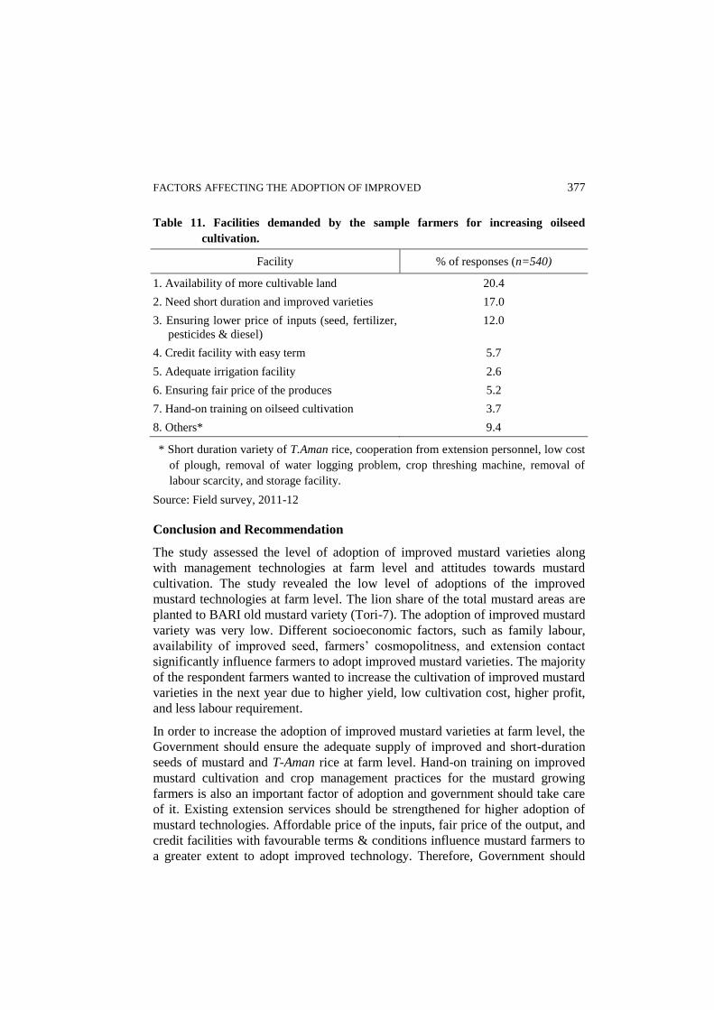
FACTORS AFFECTING THE ADOPTION OF IMPROVED 377
Table 11. Facilities demanded by the sample farmers for increasing oilseed
cultivation.
Facility % of responses (n=540)
1. Availability of more cultivable land 20.4
2. Need short duration and improved varieties 17.0
3. Ensuring lower price of inputs (seed, fertilizer,
pesticides & diesel)
12.0
4. Credit facility with easy term 5.7
5. Adequate irrigation facility 2.6
6. Ensuring fair price of the produces 5.2
7. Hand-on training on oilseed cultivation 3.7
8. Others* 9.4
* Short duration variety of T.Aman rice, cooperation from extension personnel, low cost
of plough, removal of water logging problem, crop threshing machine, removal of
labour scarcity, and storage facility.
Source: Field survey, 2011-12
Conclusion and Recommendation
The study assessed the level of adoption of improved mustard varieties along
with management technologies at farm level and attitudes towards mustard
cultivation. The study revealed the low level of adoptions of the improved
mustard technologies at farm level. The lion share of the total mustard areas are
planted to BARI old mustard variety (Tori-7). The adoption of improved mustard
variety was very low. Different socioeconomic factors, such as family labour,
availability of improved seed, farmers’ cosmopolitness, and extension contact
significantly influence farmers to adopt improved mustard varieties. The majority
of the respondent farmers wanted to increase the cultivation of improved mustard
varieties in the next year due to higher yield, low cultivation cost, higher profit,
and less labour requirement.
In order to increase the adoption of improved mustard varieties at farm level, the
Government should ensure the adequate supply of improved and short-duration
seeds of mustard and T-Aman rice at farm level. Hand-on training on improved
mustard cultivation and crop management practices for the mustard growing
farmers is also an important factor of adoption and government should take care
of it. Existing extension services should be strengthened for higher adoption of
mustard technologies. Affordable price of the inputs, fair price of the output, and
credit facilities with favourable terms & conditions influence mustard farmers to
a greater extent to adopt improved technology. Therefore, Government should
378 MIAH et al.
take appropriate steps on these aspects so that farmers become enthusiastic
toward improved mustard cultivation.
Acknowledgement
This article has been prepared from the project titled ‘Assessment of
socioeconomic impacts of oilseed research and development in Bangladesh’
funded by National Agricultural Technology Project (NATP: Phase 1), BARC,
Farmgate, Dhaka. The authors are highly grateful to BARC for funding this
project.
References
Akter, M., M.A.M. Miah, M.M.H. Khurram, M.S. Rahman and Q.M. Alam. 2010.
Economic feasibility of soybean production in some selected areas of Bangladesh.
Bangladesh Journal of Agricultural Research, 35(4): 561-571.
Akter, M., M. A. M. Miah, M. S. Rahman and M. M. H. Khurram. 2010. Adoption and
relative profitability of groundnut (Arachis hypogaea L.) cultivation in char areas of
Bangladesh. Bangladesh J. of agri. 2010, 35(1): 85-95.
Anwarul, M., Q.M. Alam and M.A. Based. 2007. Technical efficiency of mustard
production in Jamalpur district. Annual Research Report 2007-08, Oilseed Research
Centre, BARI, Joydebpur, Gazipur.
Bakr, M.A. and H.U. Ahmed. 2009. Advances in oilseed research in Bangladesh:
Proceeding of the national workshop on ‘Research and Development of Oilseed
Crops in Bangladesh and Future Challenges’, BARI, Gazipur, P. 11.
Bangladesh Bank, 2012. Monthly Economic Trends, December, 2012. Statistics
Department, Bangladesh Bank, Head Office, Dhaka, Bangladesh.
BBS, 2012. Agricultural Statistics of Bangladesh. Bangladesh Bureau of Statistics,
Ministry of Planning, Government of the People’s Republic of Bangladesh, Dhaka.
Fariduzzaman, M. 1996. An economic study of some improved varieties of mustard
production under improved managements and farmers management in some selected
areas of Bangladesh. Unpublished M.S. Thesis, Department of Agricultural
Economics, Bangladesh Agricultural University, Mymensingh.
Heisey, P., W. Tetlay, Z. Ahmad and M. Ahmad. 1990. Varietal change in post-green
revolution agriculture: empirical evidence for wheat in Pakistan. Journal of
Agricultural Economics. 44(3): 428-442.
Islam, Q. M. S., M.A.M. Miah, M.S. Rahman and M.S. Hossain. 2013. Adoption of
BARI mung varieties and its constraints to higher production in southern region of
Bangladesh. Bangladesh J. Agricultural Research, 38(1): 85-96.
Jabber, M.A. and M.S. Alam. 1993. Adoption of modern rice varieties in Bangladesh.
The Bangladesh Journal of Agricultural Economics, Vol. XVI, No. 2
FACTORS AFFECTING THE ADOPTION OF IMPROVED 379
Malik, S.J., M. Mushtaq and M.A. Gill. 1991. The role of institutional credit in the
agricultural development of Pakistan. The Pakistan Development Review. 30(4):
1039-1048.
Miah, M.A.M. and Q.M. Alam. 2008. Adoption and relative profitability of mustard
production in Bangladesh. Annual Research Report 2007-08, Oilseed Research
Centre, BARI, Joydebpur, Gazipur.
Miah, M.A.M., M. Akter, M.M.M.H. Khurram, M.A. Salam and M.A. Uddin. 2010.
Adoption of BARI mustard technology in selected areas of Bangladesh. Eco-friendly
Agriculture Journal, 3(2): 123-130, 2010.
Miah, M.A.M., M.A. Rashid and S.A.M. Shiblee. 2014. Assessment of socioeconomic
impacts of oilseed research and development in Bangladesh. Final report submitted
to the Agricultural Economics and Rural Sociology, BARC, Farmgate, Dhaka.
Mallik, M.S.A. 2013. Quality seed production of oilseed crops: An overview. Paper
presented in the workshop on ‘Modern Techniques for Quality Seed Production of
Oilseed Crops’. Oilseed Research Centre, Bangladesh Agricultural Research
Institute, Gazipur.
Salam, M.A., M.M.H. Khurram, S.M. Moniruzzaman and S. Hossain. 2011. The
economics of sesame production in two selected areas of Bangladesh. Bangladesh
Journal of Agriculture, 36(1): 117-129.
Traxler, G. and Byerlee, D. 1992. Crop management research and extension: the products
and their impact on productivity. CIMMYT Economics Paper No. 5. Mexico, D.F.:
CIMMYT.

380 MIAH et al.

ISSN 0258-7122
Bangladesh J. Agril. Res. 40(3): 381-390, September 2015
SOME BIOLOGICAL PARAMETERS OF BRINJAL SHOOT AND
FRUIT BORER, LEUCINODES ORBONALIS GUENEE (LEPIDOPTERA:
PYRALIDAE) ON POTATO IN LABORATORY CONDITION
M.A. MANNAN1, K.S. ISLAM
2, M. JAHAN
2 AND N. TARANNUM
3
Abstract
Studies were made on the biology of brinjal shoot and fruit borer (BSFB),
Leucinodes orbonalis Guenee feeding on peeled potato tubers as host in the
laboratory. It was observed that moths were active at night for mating,
oviposition and adult emergence. Adult emergence started just after sunset and it
was maximum (88.90%) during the first half of the night. Maximum mating
occurred at late night where 90.80% mating occurred in the first night of adult
emergence. Oviposition occurred in the second night of emergence when
86.62% of eggs were deposited during the first half of the night. A female laid
288.05 eggs in 2.65 days in summer and 185.55 eggs in 2.70 days in winter. The
egg hatching and larval and pupal period of BSFB were 4.13, 10.40 and 6.60
days, respectively in summer and 6.90, 14.50 and 10.65 days in winter. BSFB
needs 10.40 and 14.50 days to complete its larval period in summer and winter,
respectively. Pupal period lasted for 5-13 days. Life cycle from egg to adult was
17-44 days. The longevity of male and female adult was 3.50 and 6.20 days in
summer and 4.85 and 8.90 days in winter. Temperature in two seasons showed
variations in the biology of BSFB.
Keywords: Biology, adult longevity, brinjal shoot and fruit borer, mating,
oviposition, larval and pupal period.
Introduction
Brinjal (Solanum melongena L .) is one of the most popular and year-round
vegetable, cultivated widely in Bangladesh and covers about 15% of the total
vegetable area of the country (Rahman, 2005) with an average yield of 6.03 t/ha
(Anon, 2009). It is the leading vegetable in the country and ranks first among
summer and winter vegetables in terms of total acreage and cultivation by small
farmers, low income consumers and commercial growers. Brinjal, an
economically important commercial crop, is reported infestation by more than 36
pests (Regupathy et al., 1997) from the time of its planting to harvest. Among
them brinjal shoot and fruit borer is considered to be the most serious pest of
brinjal and it has become a very serious production constraint in all brinjal
growing countries (Alam et al., 2003). It is very difficult to control as it feeds
inside the shoots and fruits (Ghosh and Senapati, 2009). Sometimes, the yield
1Regional Agricultural Research Station, Jamalpur,
2Department of Entomology,
Bangladesh Agricultural University, Mymensingh, 3Sher-E-Bangla Agricultural
University, Dhaka, Bangladesh.
382 MANNAN et al.
loss caused by this pest has been estimated more than 85% (Rashid et al., 2003)
in Bangladesh, 85.8% (Patnaik, 2000) and 75% (Singh et al., 2005) in India.
Over 95% of farmers recognized BSFB as the most serious pest of brinjal and
nearly all of them used only chemical insecticides to combat this pest (Alam et
al., 2003).
Indiscriminate use of systemic insecticides makes the vegetables poisonous,
ecologically unsafe and economically unviable. It is easy to replace the
poisonous chemicals with the knowledge of the nature and behaviour of BSFB.
Very few farmers had knowledge on the biology of BSFB. Insect control with
insecticides and other methods is based on the availability of data on insect
biology, ecology and population dynamics. It is important to know the life cycle
of an insect so that control mechanisms may be incorporated at the most
susceptible stage of the life cycle. It is necessary to understand the biology of
BSFB for reducing crop damage. Therefore, the present study has been
undertaken to know some biological parameters of BSFB.
Materials and method
The biology of BSFB was studied during March, 2008 to April, 2009 in the
laboratory, Department of Entomology, BAU, Mymensingh, Bangladesh.
Infested fruits were collected from the unsprayed brinjal field and were kept in
tin made tray like open container with dried brinjal leaves (Plate 1). Through
completing the larval stage the full fed larvae came out from the infested brinjal
fruits and go to pupation in the dried brinjal leaves. A large number of pupae
were collected from the tray (Plate 2) and left in a glass jar. The mouth of the
glass jar was then covered with a small piece of mosquito net to allow the pupae
to develop into adults (Plate 3). After adult emergence, the male and female adult
moths were collected from the glass jars. A pair of adults (one male and one
female) was transferred into a both side open cylindrical glass jar (Plate 4)
containing a few pieces of green papers inside. The inner surface of the glass jar
was wrapped with green papers to make the environment of the jar somewhat
green like leaves of brinjal. Immediately after transferring the adults both the
open ends were covered carefully with small pored net so that the moths were not
injured during the process. Mating, adult behavior and oviposition were recorded
in the twenty same cylindrical jars. BSFB usually lays eggs on the brinjal leaves
and twigs both of which are rough surfaced. In preliminary observation it was
also evident that BSFB female prefers to deposit its eggs in a place of rough
surface. The fine meshed net was found to be a preferred surface for egg
deposition of BSFB. This type of net was used to cover the cylinder with the
objective to encourage the females to lay eggs on it. Sugar solution of 5% soaked
in cotton was placed inside the cylinder to provide nourishment for the adults
during the period of oviposition. The pair of moths was transferred to another
SOME BIOLOGICAL PARAMETERS OF BRINJAL SHOOT AND FRUIT BORER 383
similar jar after 24 hours and maintained following the same procedure. This was
continued so long the moths survived. Twenty mated females were used
separately as 20 replications for recording the egg laying trend. After removal of
adults the green papers and the fine meshed net were checked thoroughly for the
presence of BSFB egg.
Plate 1: Infested fruits with brinjal leaves.
Plate 2: Collected pupae from the tray.
Plate 3: : BSFB adult
emerged from pupae in
glass cylinder
Plate 4: One pair of adult
(male and female) within
the rearing chamber
Plate 5: Egg mass of BSFB
As expected the female laid all the eggs on the net. There was no trace of eggs on
the green papers. The eggs on the net were very tiny and visualized properly with
the help of magnifying glass. Then these were counted and it was continued until
the death of the female. This counting was done at mid night and early in the
morning as it was observed to lay eggs after sunset and no eggs were laid in day
time. After counting, the net with eggs was placed in a plastic film container and
allowed to hatch. For all the batches of eggs, the same procedure was maintained.
All the batches of eggs of an individual were added to get the fecundity of the
female. Twenty females were observed for laying their eggs (Plate 5). The age
specific egg laying pattern of the female was determined. The eggs laid by a
female per day from the 1st oviposition day to the last oviposition day were
counted daily. The longevity of the adults was recorded also.
Net with eggs were cut into several pieces carefully with minimum damage and kept in plastic film container and allowed to hatch. The eggs were observed for

384 MANNAN et al.
hatching everyday. The time of egg hatching was also recorded. Counting of the number of egg hatching was done from early in the morning to till 2.00 PM.
Once the eggs hatched into neonate larvae the duration of the incubation period was recorded. The mean incubation period and percentages of hatching were calculated. After hatching, 40 neonate larvae were released on whole peeled potato with the help of soft hair brush for feeding. Immediately after releasing on the peeled potato the newly hatched larvae were allowed to settle there. In earlier experiment laboratory rearing technique of BSFB on the peeled potato was
developed. The development of larvae of each generation was observed. Peeled potato infested with neonate larvae was observed for the development of larvae. Once the larval period is about to be completed, they came out from the host potato. The larval duration was recorded. Pre-pupae were left in a tray with dry leaves of brinjal for pupation to provide favorable environment for pupation. The pre-pupae were observed carefully for any change to become a pupa. All the pre-
pupae and pupae were left undisturbed in a tray until the adult emergence. The pupal period was recorded. The total development periods were also recorded. To study the behavior of the adult emergence a number of pupae were kept in a glass cylinder and observed for adult emergence. In a preliminary study in the laboratory it was found that adult started emerging from the pupae just after sunset and continued up to sun rising and no adults emerged in day time.
Therefore, the number of adult emergence were recorded at two times viz., mid night and early in the morning. The percentage of adult emergence was calculated at first half and second half of night.
Results and discussion
Mating behavior
BSFB moths were found active at night when the mating took place. As revealed
from the preliminary observation that maximum percentage of adult emergence
(88.90%) occurred at first half of the night (Table 1). Mating frequency was
found to vary with the adult emergence time. The percentage of mating was
90.80 in the night of adult emergence and it was 9.20 in the next night (Table 2).
The mean of mating period was 35.02 minutes in summer and 43.27 minutes in
winter (Table 3). Singh and Singh (2001a) reported mating more than once in the
life span of female which occurred at night or very early hours in the morning.
Yasuda and Kawashaki (1994) observed the copulation of male and female at
4.40 AM which lasted for 43 minutes. Das and Islam (1982) showed that the
virgin 1-day old females began calling from 18:15 to 23.45 hours and duration
was 33 minutes. Kavitha et al., (2008) showed that mating took place on the
same or next day after emergence. Prabhat and Johnsen (2000) reported that the
feeding and mating activities occurred during night and mating lasted for about
16 minutes. The findings of the above authors supported the present investigation
on mating behavior of adult moths of orbonalis L.
SOME BIOLOGICAL PARAMETERS OF BRINJAL SHOOT AND FRUIT BORER 385
Table 1. Percentage of adult emergence and oviposition of brinjal shoot and fruit
borer in different times of night.
Parameters First half of the night Second half of the night
Range Mean± SE Range Mean± SE
Adult emergence (%) 84-95 88.90±1.07 5-16 11.10± 1.07
Egg laying (%) 73.83-96.33 86.62±2.53 3.67-26.17 13.38±2.53
Table 2. Percentage of mating and ovipositing female of brinjal shoot and fruit
borer in two nights.
Parameters First night Second night
Range Mean± SE Range Mean± SE
Mating (%) 88-94 90.80±0.59 6-12 9.20±0.59
Egg laying (%) 75-98 85.90±2.88 2-25 14.10±2.88
Oviposition behaviour
Egg laying always occurred at night. Generally oviposition started during the
next night after emergence and mating. Maximum percentage of (86.62%) egg
laying occurred at first half of the night and rest of them were in the second half
of the night (Table 1). There were 85.90% females to start egg laying in the first
night and 14.10% were in the second night (Table 2). Although females were
found to survive about a week but effective egg laying period was first three
days. The eggs were distributed in mass or singly in a scattered form. A range of
40-60 eggs were found in a mass. Singh and Singh (2001b) reported that the
female laid eggs within a day or second day after mating. Singh and Singh
(2001a) reported that the laying of eggs started on the same day of mating and
continued till fourth day with an average preoviposition and ovipositional period
1.35 and 2.09 days, respectively. The number of eggs gradually decreased by
each day. The egg laying activities of the female was reported by Prabhat and
Johnsen (2000), Alam et al., (2003) and Rahman (2005). The latter author
reported that eggs were laid during the later part of the night to the early hours of
the morning. Gupta and Kauntey (2007) reported that the average oviposition
period of BSFB was 2.46 days. Harit and Shukla (2003) expressed the similar
opinion indicating that the female BSFB moth starts laying eggs on the same day
or a day after mating. The mean oviposition period was observed in this study
was 2.65 days in summer and 2.70 days in winter (Table 3). Harit and Shukla
(2003) and Gupta and Kauntey (2007) reported 2.1 and 2.46 days as oviposition
period which was similar to the present study. However, all the findings showed
that the oviposition period of BSFB is very short. This indicated that the female
emerged with full compliment of eggs which were deposited in short time
starting as early as possible.
386 MANNAN et al.
Table 3. Different biological parameters of brinjal shoot and fruit borer in two
seasons.
Parameters observed Summer Winter
Range Mean± SE Range Mean ± SE
Preoviposition period (days) 1.15-1.24 1.21±0.32 1.08-1.21 1.10±0.52
Fecundity (eggs/female) 198-387 288.05±2.32 100-281 185.55±2.52
Oviposition period (days) 1-4 2.65±0.04 1-4 2.70±0.04
Egg hatching period (days) 3.5-4.21 4.13±0.01 5.0-8.0 6.90±0.05
Egg hatching (%)
Morning 87-95 90.37±1.06 83-94 87.41±0.18
After morning to noon 5-11 9.63±1.06 4-9 12.59±0.18
Overall egg hatching (%) 80-100 94.05±0.30 28-77 60.80±0.68
Larval period (days) 8-16 10.40±0.11 11-25 14.50±0.18
Pupal period (days) 5-9 6.60±0.05 9-13 10.65±0.06
Life cycle (egg to adult) (days) 17-28 21.18±0.14 23-44 31.95±0.21
Longevity of adult (days)
Male 2-5 3.50±0.05 3-7 4.85±0.06
Female 5-8 6.20±0.05 7-11 8.90±0.07
Mating duration (minutes) 33-45 35.02±2.05 28-50 43.27±1.07
Fecundity and egg viability
After mating the female moth of L. orbonalis laid a mean of 288.05 eggs in
summer and 185.55 eggs in winter (Table 3). The overall mean percentage of egg
hatching was 94.05 (ranged from 80-100%) in summer and 60.80 (ranged from 28-
77%) in winter. The egg hatching period ranged from 3.5 to 4.21 ( x = 4.13) days in
summer and 5 to 8 ( x = 6.90) days in winter. It is important to note that eggs
hatched early in the morning. Usually in the morning 90.37% eggs hatched in
summer (5.0-7.0 AM) and 87.41% in winter (7.0-9.0 AM). Rest of the eggs
hatched at 7:00-14:00 hours in summer and 9:00-14:00 hours in winter (Table 3).
Egg laying started just after sunset and no egg was laid during day time.
Singh and Singh (2001a) reported that on an average 174.95 eggs were laid by a
female and the viability of eggs was 82.61%. Alam et al., (2003) reported that the
number of eggs laid by a female varies from 80 to 253. An adult female laid as
few as 8 to as many as 295 eggs during its lifetime with an average of 118 eggs
(PhilRice, 2007). Kavitha et al., (2008) reported that the average number of eggs
laid by an individual female was 170. The results of the present study showed
that the number of eggs laid per female and percentage of egg hatching was
higher in summer than the winter which might be due to higher temperature in

SOME BIOLOGICAL PARAMETERS OF BRINJAL SHOOT AND FRUIT BORER 387
summer. The number of eggs laid per female and percentage of egg hatching
reported by the above authors were lower than that found in summer in present
study. However, the data of fecundity in winter is similar to those of the above
reports. Environmental conditions influence the biology of many insects
including the fecundity.
Larval and pupal development
After hatching, the neonate larvae which were released on the potato tubers bored
into the tubers. They completed their larval period on this host. The neonate larva
completed its larval period in 10.40 days (8-16 days) during summer and 14.50
days (11-25 days) during winter (Table 3). Rahman (2005) showed that the larval
period was 12-15 days during summer while it was 14-22 days during winter
season. A larva of L. orbonalis completes its larval development in 15-20 days
(Talekar et al., 1999). The average larval period was 18.66 days (Singh and
Singh, 2001a), 12.80 days (Gupta and Kauntey, 2007) and 16.32 days (Kavitha et
al., 2008a). It is reported by several authors that BSFB larva completes its total
development period in 5 instars. In the present study five larval instars were
found during different activities. It became difficult to study the instar wise
developmental period in potato host as the left exuvae were not clearly visible
due to similarity with the color of potato. For this reason no attempt was made to
conduct the study on instar wise development period. Variation of larval
developmental period in summer and winter noticed in the present study was solely
the influence of higher and lower temperature in these two seasons. The effect of
different hosts such as potato used in the present study and different artificial diets
used by different authors caused such variation of larval development.
The full fed larvae moved out of the potato tubers to pupate in the supplied dried
brinjal leaves, the usual substrate for pupation. The pupal period was 6.60 days
(5-9 days) in summer and 10.65 days (9-13 days) in winter (Table 3). Rahman
(2005) showed that the pupal period was 7-10 days during summer while it was
13-15 days during winter. Almost similar pupal period was reported by Rahman
(2005) and Kavitha et al., (2008) and also by Gupta and Kauntey (2007). It is
evident from the present study and reports of other authors that BSFB needs around a
week for completion of its pupal period.
Total development period
The total development period (egg-adult) ranged from 17.0 to 28.0 days
( x =21.18) in summer and 23.0-44.0 days ( x = 31.95) in winter (Table 3).
Mathur et al., (2000) showed that the total development period was found to be
28.2±1.2 days and 37±2.31 days in summer and winter, respectively. A range of
22 to 27 days as total developmental period of brinjal shoot and fruit borer was
reported by PhilRice (2007) and a mean of 28.82 days was reported by Gupta and

388 MANNAN et al.
Kauntey (2007). Singh and Singh (2001a) described the life cycle of the brinjal
shoot and fruit borer and showed 26 to 39 days developmental period of BSFB
with 10 generations in a year. It is clear from the data that BSFB requires 1.5
times higher periods to complete its development in winter than that of summer.
Although the effect of temperature was not studied in this experiment the results
indicated that the rate of development of BSFB seemed to be directly
proportional to the temperature.
Adult emergence
Most of the adults (88.90%) emerged during the first half of the night and rest of
the adults emerged in the second half of the night (Table 1). During the day
adults remained inactive on the lower surface of the host leaf and were not
usually seen. They were found to be active at night for their mating and
oviposition purposes. At night they were mostly active from 20.00h to 22.00h
(Alam et al., 2003).
Adult longevity
Longevity of male and female of BSFB moth is shown in Table 3. The longevity of
female moth was higher than the male moth. The male adult survived in 2-5 days
( x =3.50) in summer and 3-7 days ( x =4.85) in winter. The female adult longevity
was 5-8 days ( x =6.20) in summer and 7-11 ( x =8.90) days in winter (Table 3).
Singh and Singh (2001a) reported that the male and female moth of L. orbonalis
was found to survive on an average for 3.53 days (2-5 days) and 5.80 days (2-8
days). The longevity of male and female was 4.0 days and 7.5 days, respectively
(Bang and Corey, 1991). On an average the longevity of adult was 4-8 days
reported by PhilRice (2007). Kavitha et al., (2008) reported that the longevity of
male and female was 3.50 days and 5.70 days, respectively. Reports on the
longevity of male and female BSFB moth by Kavitha et al., (2008) was 3.5 and
5.70 days, respectively which is similar to the results of the present study. As per
findings of Gupta and Kauntey (2007) the longevity of BSFB moth was very short
which is different from the results of present study as well as reports of other
authors. There might be some reasons for such short duration but no single
individual moth lived for such short period in the environmental condition of the
present study. Adult longevity was longer in winter than summer. Female
longevity was about 2-fold higher than the male.
References
Alam, S.N., Rashid, M.A., Rouf, F.M.A., Jhala, R.C., Patel, J.R., Satpathy, S.,
Shivalingaswamy, T.M., Rai, S., Wahundeniya, I., Cork, A., Ammaranan, C. and
Talekar, N.S. 2003. Development of an integrated pest management strategy for
eggplant fruit and shoot borer in South Asia. Technical Bulletin No. 28. AVRDC
SOME BIOLOGICAL PARAMETERS OF BRINJAL SHOOT AND FRUIT BORER 389
Publication Number 03-548. AVRDC-The World Vegetable Centre, Shanhua,
Taiwan. 56p.
Alam, S.N., Hossain, M.I., Rouf, F.M.A., Jhala, R.C., Patel, M.G., Raith, L.K., Sengupta,
A., Baral, K., Shylesha, A.N., Satpathy S., Shivalingaswamy, T.M., Cork, A. and
Talekar, N.S. 2006. Implemntation and promotion of an IPM strategy for control of
eggplant fruit and shoot borer in South Asia. Technical Bulletin No. 36. AVRDC
Publication Number 06-672. AVRDC-The World Vegetable Centre, Shanhua,
Taiwan. 74p.
Anonymous. 2009. Production of vegetables. Statistical Year Book of Bangladesh, BBS.
154p.
Bang, L.A. and Corey, F.M. 1991. Life history of an eggplant shoot and fruit borer,
Leucinodes orbonalis Guenee (Lepidoptera:Pyralidae). CMU J. Sci. 4(1): 45-61.
Das, G.P. and Islam, M.A. 1982. Effects of age on the calling behaviour of the brinjal
shoot and fruit borer, L. orbonalis (Lepidoptera:Pyralidae). Bangladesh J. Zool.
10(2): 120-125.
Ghosh, S.K. and Senapati, S.K. 2009. Seasonal fluctuation in the population of
Leucinodes orbonalis Guenee in the sub-himalayan region of West Bengal, India and
its control on eggplant (Solanum melongena). Prec. Agril. 10(5): 443-449.
Gupta, Y.C. and Kauntey, R.P.S. 2007. Biology of shoot and fruit borer, Leucinodes
orbonalis Guenee of brinjal, Solanum melongena Linn. at Mathura, Uttar Pradesh,
India. Asian J. Exp. Sci. 21(1): 155-160.
Harit, D.N. and Shulka, G.R. 2003. Laboratory biology of brinjal shoot and fruit borer,
Leucinodes orbonalis Guenee (Lepidoptera:Pyralidae). J. Exp. Zool. 5(2): 133-140.
Kavitha, V.S., Revathi, N. and Kingsley, S. 2008. Biology of brinjal pest, Leucinodes
orbonalis Guenee of Erode region in Tamil Nadu. J. Entomol. Res. 32(3): 255-257.
Mathur, A., Saxena, A. and Jain, L.V. 2000. The seasonal effects on the biology of
Leucinodes orbonalis Guenee during summer and winter. Asian J. Exp. Sci.
13(1&2): 1-4.
Patnaik, H.P. 2000. Flower and fruit infestation by brinjal shoot and fruit borer,
Leucinodes orbonalis Guenee–damage potential vs. weather. Veg. Sci. 27(1): 82-83.
PhilRice. 2007. Integrated pest management in rice-vegetable cropping systems.
Maligaya, Science City of Munoz, Nueva Ecija. 73p.
Prabhat, K. and Johnsen, S. 2000. Life cycle studies on fruit and shoot borer (Leucinodes
orbonalis) and natural enemies of insect pests of eggplant (Solanum melongena).
J. Appl. Biol. 10(2): 178-184.
Rahman, M.M. 2005. IPM technologies of different crops potential for field trial
generated at the Department of Entomology, BSMRAU, Gazipur. Paper presented at
IPM operation workshop organized by the DANIDA-DAE-SPPS project and held on
March 30 at DAE, Khamarbari, Dhaka, Bangladesh.
Rashid, M.A., Alam, S.N., Rouf, F.M.A. and Talekar, N.S. 2003. Socio economic
parameters of brinjal pest control in Jessore district of Bangladesh. Technical

390 MANNAN et al.
Bulletin No. 29. Shanbua, Taiwan. AVRDC-The world vegetable centre. AVRDC
publication No. 03-556. 29p.
Regupathy, A., Armes, N.J., Asoken, G., Jadhav, D.R., Soundarajan, R.D. and Russell,
D.A. 1997. Best method for insecticide resistance management of Helicoverpa
armigera. In: International Conference on Integrated Approach to Combating
Resistance. A.L. Devonshine (ed.), April 14-16, 1997. IACR, Rothamsted,
Harpendle, UK. 116p.
Singh, N.P., Thakur, N.S.A., Shyclesha, A.N. and Biswas, S. 2005. Implementation and
Promotion of IPM technology for the control of eggplant shoot and fruit borer
(Leucinodes orbonalis Guenee) in Meghalaya and Tripura. Publication No.-17.
AVRDC, Post Box: 42, Sanghua, Taiwan 741.
Singh, Y.P. and Singh, P.P. 2001a. Biology of shoot and fruit borer (Leucinodes
orbonalis Guenee) of eggplant (Solanum melongena L) at medium high altitude hills
of Meghalaya. Indian J. Entomol. 63(3): 360-368.
Singh, Y.P. and Singh, P.P. 2001b. Lab biology of shoot and fruit borer (Leucinodes
orbonalis Guenee) of eggplant at medium high altitude hills of Meghalaya.
Indian J. Entomol. 63(4): 373-376.
Talekar, N.S., Lin, M.Y. and Hwang, C.C. 1999. Rearing eggplant fruit and shoot borer.
A slide set and illustrated guide. AVRDC publication no. 99-486, April 1999.
AVRDC, PO Box 42, Shanhua, Taiwan 741 ROC. 12p. (Text in Ent) (AVRDC staff
publication) (SB348. ESREP-102).
Yasuda, K. and Kawasaki, K. 1994. Mating behaviour of eggplant fruit borer, Leucinodes
orbonalis Guenee (Lepidoptera:Pyralidae) and capture of males in virgin female
traps. Japanese J. Appl. Entomol. Zool. 38(4): 302-304.

ISSN 0258-7122
Bangladesh J. Agril. Res. 40(3): 391-398, September 2015
EFFICACY OF FUNGICIDES IN CONTROLLING BOTRYTIS
GRAY MOLD OF CHICKPEA (Cicer arietinum L.)
M SHAHIDUZZAMAN1
Abstract
A field experiment was carried out at Regional Pulses Research Station (RPRS),
Madaripur during Rabi season of 2011-12 and 2012-13 to evaluate the most
effective fungicides in controlling Botrytis Gray Mold (BGM) of Chickpea. Five
different fungicides e.g. Propiconazole (Tilt 250 EC), Carbendazim (Bavistin
DF), Fenamidone+Mancozeb (Secure 600 WG), Difenoconazole (Score 250
EC), Tebuconazole (Folicure 250 EC) were evaluated under natural condition.
Results revealed that among the five fungicides Fenamidone+Mancozeb (Secure
600WG) sprayed at the rate of 1g/L with 7 days interval gave the lowest BGM
score of 3.80 and 4.00 in 1-9 scale during 2011-12 and 2012-13 and produced
highest yield of 1547 and 1443 kg/ha, respectively. Besides, the highest BGM
was scored by the untreated control plot (6.26 and 6.33) and produced the lowest
yield of 988 and 853 kg/ha during the two consecutive years.
Introduction
Chickpea (Cicer arietinum L.) is the third most important pulse crop in the world
and seven most important pulse crops in Bangladesh as per production. Botrytis
gray mold (BGM) caused by Botrytis ceneria is an important disease of chickpea
in northern India, Nepal, Bangladesh and Pakistan. It was first reported in India
in 1915 (Shaw and Ajrekar, 1915). Outside the Indian subcontinent the disease
has been reported from Argentina (Carranza, 1965), Australia (Nene et al., 1989),
Canada (Kharbanda and Bernier, 1979), and Chile (Sepulveda and Alvarez,
1984). It was first documented in 1981 in Bangladesh (Annon., 1981). In
Bangladesh, for high infestation of BGM, farmers are reluctant to grow chickpea
that results declining of area and production of the crop. The pathogen of the
disease is soil, seed and air borne. Different researchers had been taking many
efforts to control the disease. Foliar application of fungicides is one of the most
important management options to control the disease. Therefore, the experiment
has been conducted to find out suitable fungicide to control BGM of chickpea.
Materials and Method
The experiment was conducted at Regional Pulses Research Station (RPRS),
Madaripur, Bangladesh during Rabi season of 2011-12 and 2012-13. The
experiment was laid out in Randomized Complete Block Design (RCBD) with
1Scientific Officer, Regional Pulses Research Station, Bangladesh Agricultural Research
Institute (BARI), Madaripur, Bangladesh.
392 SHAHIDUZZAMAN
three replications. The five fungicides viz- Propiconazole (Tilt 250 EC, 0.5
ml/L), Carbendazim (Bavistin DF, 2.0 g/L), Fenamidone+Mancozeb (Secure 600
WG, 1 g/L), Difenoconazole (Score 250 EC, 0.5 ml/L), Tebuconazole (Folicure
250EC, 2.0 ml/L) and untreated control were included in the study. The unit plot
size was 2.4m × 3m and plant spacing was 50 cm × 10 cm. The seeds of BGM
susceptible chickpea variety BARI Chola-1 (Nabin) was treated with Provax-200
to control fusarium wilt and sown on 16 November 2011 and 14 November 2012.
Intercultural operations were done manually and herbicides application (Rahman
and Miah, 1989). The experiment was monitored regularly to observe the first
appearance of BGM. Spraying of fungicides was started when the disease
appeared on the crop. Four sprays were applied at weekly interval on 8, 15, 22
and 27 February, 2012 and 3, 10, 17 and 24 February, 2013 respectively by the
knapsack sprayer. Data on BGM disease was recorded on three frequencies (18,
25 and 30 February, 2012 and 13, 20 and 27 February, 2013). BGM of chickpea
was graded on a 1-9 scoring scale (Singh, 1999). The scale described as 1= no
infection on any part of the plant, 2= minute lesions on lower leaves, flowers and
pods covered under dense plant canopy, usually not visible, 3= lesions on less
than 5% of the leaves, flowers and pods covered and under dense plant canopy,
4= lesions and some fungal growth (conidiophores and conidia) can be seen on
up to 15% of the leaves, flowers and pods and branches covered under dense
plant canopy, 5= lesions and slight fungal growth on up to 25% of the leaves,
flowers and pods, stems and brunches covered under dense plant canopy, 6=
lesions and fungal growth on up to 40% of the leaves, flowers and pods, stems
and branches defoliation, 25% of the plant killed, 7= large lesions and good
fungal growth on up to 60% of the leaves, flowers and pods, stems and branches
defoliation common, drying of branches and 50% of the plants killed, 8= large
lesions and profuse fungal growth on up to 80% of the leaves, flowers and pods,
stems and branches, severe defoliation, drying of branches and 75% of the plants
killed, 9= large lesions, very profuse fungal growth on up to 100% of the flowers,
pods, stems, branches, almost complete defoliation, drying of plants and 100% of
the plants killed. The crop was harvested on 15 March 2012 and 18 March 2013
at matured stage. Data on yield contributing characters recorded from 10
randomly selected plants from each plot. Grain yield (kg/ha) were recorded from
the whole plot. The Data were analyzed statistically through MSTAT-C.
Results and Discussion
The fungicides caused sharp variation in percent mortality and severity of
botrytis gray mold disease of chickpea in Madaripur during 2011-12 (Table 1).
Maximum percent mortality (15.35) was observed in Tebuconazole (Folicur
250EC) treated plot and minimum (7.65) in Difenoconazole (Score 250EC)

EFFICACY OF FUNGICIDES IN CONTROLLING BOTRYTIS 393
treated plot. The BGM disease score was found minimum (3.80) in
Fenamidone+Mancozeb (Secure 600 WG) treated plot and maximum (6.26) in
control plot. The grain yield and yield contributing characters of chickpea were
significantly influenced by the test fungicides during 2011-12 cropping season
(Table 2). The highest number of branches (4.25) were recorded from
Propiconazole (Tilt 250 EC), Fenamidone+Mancozeb (Secure 600 WG) and
Tebuconazole (Folicur 250EC) treated plots and lowest (3.20) from
Difenoconazole (Score 250 EC) treated plot. Similarly, the highest plant height
(45.00cm) was recorded from Difenoconazole (Score 250 EC) treated plot and
lowest (33.33 cm) from Tebuconazole (Folicur 250 EC) treated plot. There was
no significant differences in pods/plant and seeds/pod due to the application of
fungicides in chickpea. However, higher number of pods/plant was observed in
case of fungicide treatment over untreated control plot. In case of seeds/pod,
Fenamidone+Mancozeb (Secure 600 WG) treated plot produced maximum (1.78)
while control plot produced lowest (1.53) seeds/pod. The effect of fungicide was
statistically similar in respect of 100 seed weight but differed from the untreated
control plot. The 100 seed weight ranged from 11.5-13.0 g among the fungicide
treated plot and maximum (13.0 g) was in Fenamidone+Mancozeb (Secure 600
WG) treated plot and minimum (8.9 g) in control plot. Among the five fungicides
Fenamidone+Mancozeb (Secure 600 WG) sprayed plot produced highest seed
yield (1547 kg/ha) which was statistically similar to that of Propiconazole (Tilt
250 EC) and Difenoconazole (Score 250EC) while the lowest (988 kg/ha) yield
was recorded in control plot (Table 2).
Table 1. Efficacy of different fungicides in controlling BGM of chickpea during
2011-12 at Madaripur.
Fungicides Mortality (%) BGM Scale
(1-9)
Propiconazole (Tilt 250 EC) 9.45 4.73
Carbendazim (Bavistin DF) 8.36 4.76
Fenamidone+Mancozeb (Secure 600 WG) 9.82 3.80
Difenoconazole (Score 250 EC) 7.65 5.00
Tebuconazole (Folicur 250 EC) 15.35 5.33
Control 11.46 6.26
CV(%) 8.85 5.96
LSD (0.05) 5.80 0.53
Values within a column having same letter(s) do not differ significantly (p=0.05);
BGM=Botrytis gray mould.

394 SHAHIDUZZAMAN
Ta
ble
2.
Eff
ect
of
dif
feren
t fu
ng
icid
es o
n t
he
yie
ld a
nd
yie
ld c
on
trib
uti
ng
ch
ara
cter
s o
f ch
ick
pea
th
rou
gh
su
pp
ress
ion
of
BG
M
du
rin
g 2
01
1-1
2 a
t M
ad
ari
pu
r.
Fu
ng
icid
es
Bra
nch
per
pla
nt
Pla
nt
hei
ght
(cm
) P
od
s p
er p
lant
See
ds
per
po
d
10
0 s
eed
wei
ght
(gm
) Y
ield
(kg/h
a)
Pro
pic
onaz
ole
(T
ilt
25
0 E
C)
4.2
5 a
4
1.3
3 b
4
7.5
3
1.7
3
12
.0a
15
14
ab
Car
ben
daz
im (
Bav
isti
n D
F)
3.6
6 a
4
2.2
0 a
b
41
.80
1
.33
12
.5 a
1
43
3 b
Fen
am
ido
ne+
Manco
zeb
(S
ecu
re 6
00 W
G)
4.2
5 a
3
6.8
0 c
4
7.9
3
1.7
8
13
.0 a
1
54
7 a
Dif
eno
conaz
ole
(S
core
25
0 E
C)
3.2
0 b
4
5.0
0 a
4
2.6
7
1.6
6
12
.2 a
1
49
2 a
b
Teb
uco
naz
ole
(F
oli
cur
25
0 E
C)
4.2
5 a
3
3.3
3 c
4
6.3
3
1.5
6
11
.5 a
1
10
6 c
Co
ntr
ol
3.8
0 a
3
6.8
0 c
3
8.5
3
1.5
3
8.9
b
98
8 d
CV
(%)
7.7
1
10
.32
11
.13
1
2.4
1
8.0
5
4.0
7
LS
D (
0.0
5)
1.5
6
6.8
83
10
.18
0
.65
43
.30
96
.35
Val
ues
wit
hin
a c
olu
mn
havin
g s
am
e le
tter
(s)
do
no
t d
iffe
r si
gn
ific
antl
y (
p=
0.0
5).
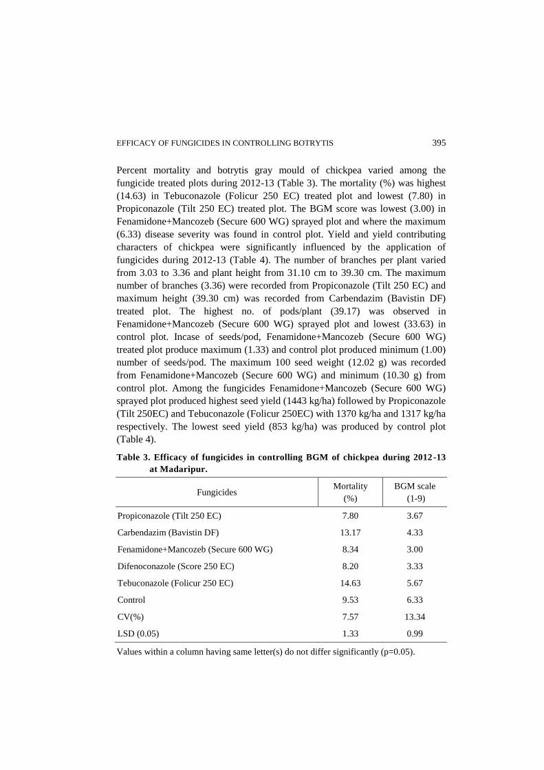
EFFICACY OF FUNGICIDES IN CONTROLLING BOTRYTIS 395
Percent mortality and botrytis gray mould of chickpea varied among the
fungicide treated plots during 2012-13 (Table 3). The mortality (%) was highest
(14.63) in Tebuconazole (Folicur 250 EC) treated plot and lowest (7.80) in
Propiconazole (Tilt 250 EC) treated plot. The BGM score was lowest (3.00) in
Fenamidone+Mancozeb (Secure 600 WG) sprayed plot and where the maximum
(6.33) disease severity was found in control plot. Yield and yield contributing
characters of chickpea were significantly influenced by the application of
fungicides during 2012-13 (Table 4). The number of branches per plant varied
from 3.03 to 3.36 and plant height from 31.10 cm to 39.30 cm. The maximum
number of branches (3.36) were recorded from Propiconazole (Tilt 250 EC) and
maximum height (39.30 cm) was recorded from Carbendazim (Bavistin DF)
treated plot. The highest no. of pods/plant (39.17) was observed in
Fenamidone+Mancozeb (Secure 600 WG) sprayed plot and lowest (33.63) in
control plot. Incase of seeds/pod, Fenamidone+Mancozeb (Secure 600 WG)
treated plot produce maximum (1.33) and control plot produced minimum (1.00)
number of seeds/pod. The maximum 100 seed weight (12.02 g) was recorded
from Fenamidone+Mancozeb (Secure 600 WG) and minimum (10.30 g) from
control plot. Among the fungicides Fenamidone+Mancozeb (Secure 600 WG)
sprayed plot produced highest seed yield (1443 kg/ha) followed by Propiconazole
(Tilt 250EC) and Tebuconazole (Folicur 250EC) with 1370 kg/ha and 1317 kg/ha
respectively. The lowest seed yield (853 kg/ha) was produced by control plot
(Table 4).
Table 3. Efficacy of fungicides in controlling BGM of chickpea during 2012-13
at Madaripur.
Fungicides Mortality
(%)
BGM scale
(1-9)
Propiconazole (Tilt 250 EC) 7.80 3.67
Carbendazim (Bavistin DF) 13.17 4.33
Fenamidone+Mancozeb (Secure 600 WG) 8.34 3.00
Difenoconazole (Score 250 EC) 8.20 3.33
Tebuconazole (Folicur 250 EC) 14.63 5.67
Control 9.53 6.33
CV(%) 7.57 13.34
LSD (0.05) 1.33 0.99
Values within a column having same letter(s) do not differ significantly (p=0.05).

396 SHAHIDUZZAMAN
Ta
ble
4.
Eff
ect
of
dif
feren
t fu
ng
icid
es o
n t
he
yie
ld a
nd
yie
ld c
on
trib
uti
ng
ch
ara
cter
s o
f ch
ick
pea
th
rou
gh
su
pp
ress
ion
of
BG
M
du
rin
g 2
01
2-1
3 a
t M
ad
ari
pu
r.
Fu
ng
icid
es
No
. o
f b
ranch
es
/pla
nt
Pla
nt
hei
ght
(cm
)
No
. o
f p
od
s/
pla
nt
No
. o
f se
eds/
po
d
10
0 s
eed
wt.
(g)
Yie
ld
(kg/h
a)
Pro
pic
onaz
ole
(T
ilt
25
0 E
C)
3.3
6a
38
.37
a
38
.10
a 1
.23
ab
12
.00 a
1
37
0 a
b
Car
ben
daz
im (
Bav
isti
n D
F)
3.2
3ac
3
9.3
0a
37
.67
a 1
.23
ab
11
.63 a
1
17
5 b
c
Fen
am
ido
ne+
Manco
zeb
(S
ecu
re 6
00 W
G)
3.3
3ab
3
8.9
0a
39
.17
a
1.3
3 a
1
2.0
2 a
1
44
3 a
Dif
eno
conaz
ole
(S
core
25
0 E
C)
3.0
3d
38
.47
a 3
8.1
7a
1.2
7 a
1
1.8
3 a
1
04
8 c
d
Teb
uco
naz
ole
(F
oli
cur
25
0 E
C)
3.1
3cd
3
1.1
0c
3
3.7
7b
1
.07
c
10
.83 b
1
31
7 a
b
Co
ntr
ol
3.3
3ab
3
3.3
0b
33
.63b
1
.00
c
10
.30 b
8
53
e
CV
(%)
2.9
1
2.4
3
2.7
2
6.4
0
3.6
2
8.7
9
LS
D (
0.0
5)
0.1
6
1.5
5
1.7
4
0.1
3
0.7
2
73
.6
Val
ues
wit
hin
a c
olu
mn
havin
g s
am
e le
tter
(s)
do
no
t d
iffe
r si
gn
ific
antl
y (
p=
0.0
5).
EFFICACY OF FUNGICIDES IN CONTROLLING BOTRYTIS 397
Management of plant diseases successfully achieved through application of
chemical fungicides. All the tested fungicides reduced the disease score and
enhanced plant growth parameters and yield of chickpea in comparison with
control plot. The lowest BGM disease score of 3.80 and 3.00 were recorded from
the plots sprayed with Fenamidone+Mancozeb (Secure 600 WG) and the highest
score of 6.26 and 6.33 were recorded from control plot during 2011-12 and 2012-
13, respectively. In 2012-13, the yield of chickpea was less than that of 2011-12
due to attack of pod borer (Helicoverpa armigera Hubner). This results in less
number of seed/pod in 2012-13. But the BGM infection was comparatively less
in the second year due to unfavorable climatic conditions for BGM results in low
scoring scale. However, foliar sprays, used at regular intervals with the first
appearance of the disease, can control an epidemic in the crop (Pande et al.,
2002), particularly when used in combination with a seed-dressing fungicide
(Grewal and Laha, 1983). Effective fungicides used as a foliar spray 50 days
after sowing or with the first sign of the disease include Captan, Carbendazim,
Chlorothalonil, Mancozeb, Thiabendazole, Thiophanate-methyl, Thiram,
Triadimefon, Triadimenol, or Vinclozolin (Singh and Kaur, 1990; Haware and
McDonald, 1992; Bakr et al., 1993; Haware, 1998; Knights and Siddique, 2002;
Pande et al., 2002; Davidson et al., 2004). Sometimes multiple sprays are
recommended, although generally one spray at flowering followed by another 10
days later on a moderately resistant chickpea cultivar provides the best protection
against BGM on chickpea (Pande et al., 2002).
Conclusion
Fenamidone+Mancozeb (Secure 600 WG) at 1 g/L water effectively controlled
the BGM disease and produced higher yield of chickpea through four sprays at 7
days interval if applied at the first appearance of the disease.
References
Annonymous. 1981. Annual Report of the Regional Agricultural Research Station,
Ishwrdi, Bangladesh, 1980-81. Pp. 66.
Bakr, M. A., M. M. Rahman, F. Ahmed and J. Kumar. 1993. Progress in management of
botrytis gray mold of chickpea in Bangladesh. In ‘Recent advances in research in
botrytis gray mold of chickpea’. (Eds M, P. Haware, C. L. L. Gowda, D. McDonald)
pp. 17–19. (ICRISAT: Patancheru, AP, India)
Carranza, J. M. 1965. [Wilt of chickpea (C. arietinum) caused by B. cinerea.] (In Es.).
Revta Fac. Agron. Univ. Nac. La Plata. 41:135-138.
Davidson, J. A., S. Pande, T. W. Bretag, K. D. Lindbeck and G. K. Kishore. 2004.
Biology and management of Botrytis spp. in legume crops. In ‘Botrytis: biology,
pathology and control’. (Eds Y. Elad, B. Williamson, P. Tudzynski, N. Delen) pp.
295–318. (Kluwer Academic Publishers: The Netherlands)

398 SHAHIDUZZAMAN
Grewal, J. S. and S. K. Laha. 1983. Chemical control of botrytis blight of chickpea.
Indian J. Phytopath. 36: 516–520.
Haware, M. P. 1998. Diseases of chickpea. In ‘The pathology of food and pasture
legumes’. (Eds D. J. Allen and J. M. Lenne) Pp. 473–516. (ICARDA, CAB
International: Wallingford, UK)
Haware, M. P. and D. McDonald. 1992. Integrated management of botrytis gray mold of
chickpea. In ‘Botrytis gray mold of chickpea’. (Eds M. P. Haware, D. G. Faris and C.
L. L. Gowda.) Pp. 3–6. (ICRISAT: Patancheru, AP, India)
Kharbanda, P. D. and C. C. Bernier. 1979. Botrytis gray mold of chickpea in Mani toba.
Plant Disease Reporter 63(8): 662-663.
Knights, E. J. and K. H. M. Siddique. 2002. Manifestation of Botrytis cinerea on
chickpeas in Australia. In ‘Workshop Proceedings Integrated Management of
Botrytis Grey Mould of Chickpea in Bangladesh and Australia’. Pp. 70–77.
(Bangladesh Agricultural Research Institute: Joydebpur, Gazipur, Bangladesh)
Nene, Y. L., V. K. Sheila and S. B. Sharma. 1989. A world list of chickpea (Cicer
arietinum L.) and pigeonpea (Cajanus cajan L Mill sp.) pathogens. Pulse Pathology
Progress Report No. 32. Patancheru, A.P. 502 324, India: International Crops
Research Institute for the Semi-Arid Tropics. Pp. 19.
Pande, S., G. Singh, J. N. Rao, M. A. Bakr, P. C. P. Chaurasia, S. Joshi, C. Johansen, S.
D. Singh, J. Kumar, M. M. Rahman, and C. L. L. Gowda. 2002. Integrated
management of botrytis gray mold of chickpea. Information Bulletin No. 61,
ICRISAT, Andhra Pradesh, India.
Rahman, M. A. and A. A. Miah. 1989. Study on seedling mortality and plant competition
of lentil at a wide range of population densities. Research Report on Pulse
Agronomy. Pulse Research Center. BARI, Joydebpur, Gazipur. P. 27-33
Sepulveda, R. P. and A. M. Alvarez. 1984. Identification of Botrytis cinerea Pers.
causing blight in chickpea (Cicer arietinum L.) (In Es.) Agricultural Technica.
44:79-80.
Shaw, F. J. F. and S. L. Ajrekar. 1915. The genus Rhizoctonia in India. Botanical Series
7:77. Memoirs of Department of Agriculture, New Delhi, India.
Singh, G. 1999. Proposed rating scale for BGM of chickpea. BGM Newsletter 2(1): 5-6
Singh, G. and L. Kaur. 1990. Chemical control of gray mold of chickpea. Plant Dis. Res.
5: 132–137.
ISSN 0258-7122
Bangladesh J. Agril. Res. 40(3): 399-407, September 2015
BRINJAL SHOOT AND FRUIT BORER INFESTATION IN RELATION
TO PLANT AGE AND SEASON
M. A. MANNAN1, K. S. ISLAM
2 AND M. JAHAN
2
Abstract
Brinjal shoot and fruit borer infestation varied significantly in relation to plant
age and season. The peak shoot infestation was 8.56% in the 10th
week of
transplanting. No infestation of BSFB was found up to 5 weeks of transplanting.
The shoot infestation was initiated in the 6th
week of transplanting which
increased to a little higher level in the next week. Then it showed an exponential
increase of shoot infestation up to 10th
week after which it declined steadily.
Flowering and fruit setting started in the 9th
week of transplanting. Infestation of
brinjal shoot and fruit borer (BSFB) shifted to fruits from shoots causing a
steady declined in the trend of shoot infestation. Plant age had significant effect
(r2=0.87) on fruit infestation. The fruit infestation reached the highest level
(38.56%) in 14th
week of transplanting. However, the level of infestation at
different ages of the plant may vary depending on the location, temperature,
variety etc. The shoots and fruits of brinjal plant were found to be infested by
BSFB throughout the year, although the level of infestation varied. Maximum
shoot and fruit infestation was found in the month of September.
Keywords: Brinjal shoot and fruit borer, Leucinodes orbonalis, infestation,
plant age, seasonal fluctuation.
Introduction
Brinjal is a versatile and economically important vegetable among small-scale
farmers and low income consumers of the entire universe (FAO, 2000). It is the
leading vegetable in the country and ranks first among summer and winter
vegetables in terms of total acreage. Asia has the largest brinjal production which
comprises about 90% of the total production area and 87% of the world
production (FAO, 2000). Brinjal, an economically important commercial crop, is
reported variedly to be infested by more than 36 pests (Regupathy et al., 1997)
from the time of its planting to harvest. Among them, brinjal shoot and fruit borer
(BSFB), Leucinodes orbonalis Guenee is considered to be the most serious pest
of brinjal and it has become a very serious production constraint in all brinjal
growing countries (Alam et al., 2003). The brinjal shoot and fruit borer is the key
insect pest of brinjal in Bangladesh (Alam and Sana, 1964), India (Tewari and
Sardana, 1990) and other countries of the world (Dhankar, 1988). The fruit
infestation by this pest may be as high as 67% (BARI 1991). It is very difficult to
control since it feeds inside the shoots and fruits (Ghosh and Senapati, 2009).
1Regional Agricultural Research Station, Jamalpur.
2Department of Entomology,
Bangladesh Agricultural University, Mymensingh, Bangladesh.

400 MANNAN et al.
Over 95% farmers recognized BSFB as the most serious pest and nearly all of
them used only chemical insecticides to combat (Alam et al., 2003). Sometimes,
the yield loss caused by this pest has been estimated more than 85% (Rashid et
al., 2003) and 86% (Ali et al., 1996) in Bangladesh, 85.8% (Patnaik, 2000), 75%
(Singh et al., 2005) and 95% (Naresh et al., 1986) in India. Brinjal production is
seriously affected by damage caused by brinjal shoot and fruit borer (AVRDC,
2001). The management practices mainly include spraying different insecticides
which cause several pesticide related complications and leave toxic residues in
the fruits, reduce the beneficial arthropods and create pollution of the
environment. The vegetable growers of Jessore region spray insecticide almost
every day or every alternate day in the brinjal field with as many as 84 times in a
season (BARI, 1994). It is now urgently required to find out an alternative and
non-insecticidal method for controlling this pest. Frequent use of systemic
insecticides makes the vegetables poisonous, ecologically unsafe and
economically unviable. It is easy to replace the poisonous chemicals with
knowledge through transplanting the seedlings at appropriate time and
understanding the knowledge of seasonal fluctuation of temperature and other
abiotic factors. Very few farmers had knowledge on the infestation status of
BSFB in relation to plant age and seasonal fluctuation of temperature. Therefore,
the present study was undertaken to know the effects of plant age of brinjal and
seasonal variation on the infestation of BSFB.
Materials and method
An experiment was conducted in the field of Entomology Division, Bangladesh
Agricultural University, Mymensingh during September 2008 to October 2009
on the incidence of BSFB in relation to plant age and season. The seedlings were
raised in a seed bed. Variety was BARI Begoon 8. The land was prepared by
ploughing and laddering and fertilized with organic manure such as cow dung @
10 m ton/ha, 7 days before final land preparation and chemical fertilizer Urea @
150 kg/ha, TSP @ 100 kg/ha and MP @ 150 kg/ha. The whole TSP and MP and 1/3 of Urea were applied during the final land preparation. Rest of the Urea was
applied in two splits- one 30 days and other 50 days after planting. The
individual plot size was 4.5m 4.2m. The seedlings were planted in September
2008 and March 2009 with spacing 75 cm in between lines and 60 cm in between
plants. Irrigation and other cultural operations were done as and when necessary.
Ten plots were made for recording data and each plot was treated as one
replication. No control measure was taken except the removal of shoots and fruits
at the time of data collection. Infestation of BSFB to the shoots and fruits was
monitored weekly after establishment of the plant in the field and continued to
the last harvest of the brinjal fruits. Shoot damage was recorded by counting the
infested shoots from 10 randomly selected plants. Percentage of shoot damage
was calculated from damaged and healthy shoots. The number of infested and

BRINJAL SHOOT AND FRUIT BORER INFESTATION IN RELATION 401
healthy brinjal fruits per plot were recorded at each harvest. The percentage of
infestation by number was calculated using the number of infested and total
brinjal fruits. At each count the affected shoots and fruits were removed and
harvested. Incidence of BSFB in different months was calculated from the pooled
weekly data. The correlations between seasonal incidence and environmental
factors such as temperature, humidity and rainfall were determined.
Results and Discussion
Infestation level of BSFB with plant age: After transplanting the brinjal
seedlings, it was monitored weekly for BSFB infestation. Infestation by BSFB
was different in plant of different ages (Figure 1). The peak shoot infestation was
8.56% in the 10th week of transplanting. No infestation of BSFB was found up to
5 weeks of transplanting. The shoot infestation was initiated in the 6th week of
transplanting which increased to a little higher level in the next week. Then it
showed an exponential increase of shoot infestation up to the 10th week after
which it declined steadily. Flowering and fruit setting started in the 9th week.
Infestation of BSFB shifted to fruits from shoots causing a steady decline in the
trend of shoot infestation. There was no significant correlation (r2=0.17) between
plant age and shoot infestation.
Figure 1. Effect of plant age on the infestation of L. orbonalis
On the other hand, plant age had significant effect (r2=0.87) on fruit infestation
which started in 9th week of transplanting and showed 5.13% infestation. Then
the fruit infestation increased rapidly showing a distinct increasing trend. The
fruit infestation reached to its highest level (38.56%) in 14th week of
402 MANNAN et al.
transplanting. Thereafter, a little decline of fruit infestation was observed. It is
evident that older plants suffered far more from the attack of BSFB and caused
higher damage to the brinjal plants especially to the fruits. However, the level of
infestation at different ages of the plant may vary depending on the location,
temperature, variety etc. Therefore, in the early stage of the plant growth the pest
BSFB is not a serious problem to brinjal cultivation. The management option
should be selected depending on the level of BSFB infestation. In general, the
brinjal growers may not need to adopt any chemical control measures until the
plant reaches its maximum vegetative stage or pre-flowering stage as the
commencement of infestation is noticed during that stage.
Several authors reported that the infestation of BSFB depends on plant age.
Hossain et al., (2002) reported that plant age had significant effect on the
incidence of brinjal shoot and fruit borer. They showed the highest infestation
(32.80%) of BSFB at 70 days after transplanting which was statistically different
from the infestation (5.18%) at 40 days after transplanting. They also reported
that the rate of infestation gradually increased with the increase of plant age and
then decreased in 100 days (31.70%) after transplanting. Naik et al., (2008)
showed the initial infestation of BSFB at 51 days after transplanting and
thereafter the infestation gradually increased from 10.2 to 82.4% of shoot
damage. It required 74 days after transplanting to reach a peak incidence of
BSFB. Thereafter declined gradually with rise in temperature. In the present
study the maximum shoot damage was found as 8.56% while Sharma and
Chhibber (1999) reported that shoot damage was 15.89% at 29 days after
transplanting of brinjal. The present finding on BSFB shoot infestation is
different from the reports of Sharma and Chhibber (1999). It is noted that BSFB
needs good vegetative growth of the plants for its infestation.
The level of BSFB infestation reported by Hossain et al., (2002) was 31.70% at
100 days after transplanting which is similar to the results of present study as it
was recorded 31.25% fruit infestation at 91 days (13 weeks) after transplanting.
The initial infestation of BSFB reported by Naik et al., (2008) was 51 days after
transplanting which was near to 42 days (6 weeks) in the present study. The
maximum shoot infestation was observed at 70 days (10 weeks) after
transplanting in the present study which was also supported by Naik et al., (2008)
although the level of infestation was different.
The results of the present study and the findings of above authors clearly indicate
that the infestation of BSFB has relationship with the plant age showing higher
pest incidence with the progress of plant growth. In other words, it can be said
that infestation level is higher with sufficient vegetative growth of the plant and
the presence of fruiting bodies.

BRINJAL SHOOT AND FRUIT BORER INFESTATION IN RELATION 403
Seasonal incidence of L. orbonalis
The seasonal incidence of BSFB throughout the year in terms of shoot and fruit infestation is shown in Figure 2. Observation on the seasonal incidence of BSFB started in the month of September 2008 and continued up to October 2009. It was found that the level of fruit infestation was always higher than that of shoot infestation. The shoots and fruits of brinjal plant were found to be infested by BSFB throughout the year although the level of infestation varied. The shoot infestation was only 1.33% in January which was very similar in February. Then it started to increase steadily up to the month of September when maximum shoot infestation was observed. Then a marked decline was observed in October which showed a further slow decline thereafter up to the month of December.
Figure 2. Seasonal incidence of L. orbonalis in unsprayed brinjal field
The incidence of BSFB in fruits was calculated on the basis of the infestation of
marketable size of the fruits. The fruit infestation was found 5.26% in the month
of January which was minimum. Then a slight increase was found in the month
of February which followed a sharp increase in March reaching 31.27%.
Thereafter the infestation of fruit was found to show a more or less steady
increase up to the month of September when it reached its peak (56.38%). Then a
certain drop of infestation level occurred in the next month and reached to a
significantly lower level as the winter progressed. In the month of December the
level of infestation was found 12.25%.
In addition, it was observed that a large number of flowers, flower buds and very
young fruits were infested and damaged totally which were not included in the
data. If they were included the level of fruit infestation would be much higher as
it is evident in the Figure 3. The variation of BSFB infestation in shoots and
fruits might be due to several abiotic and biotic factors. The temperature and
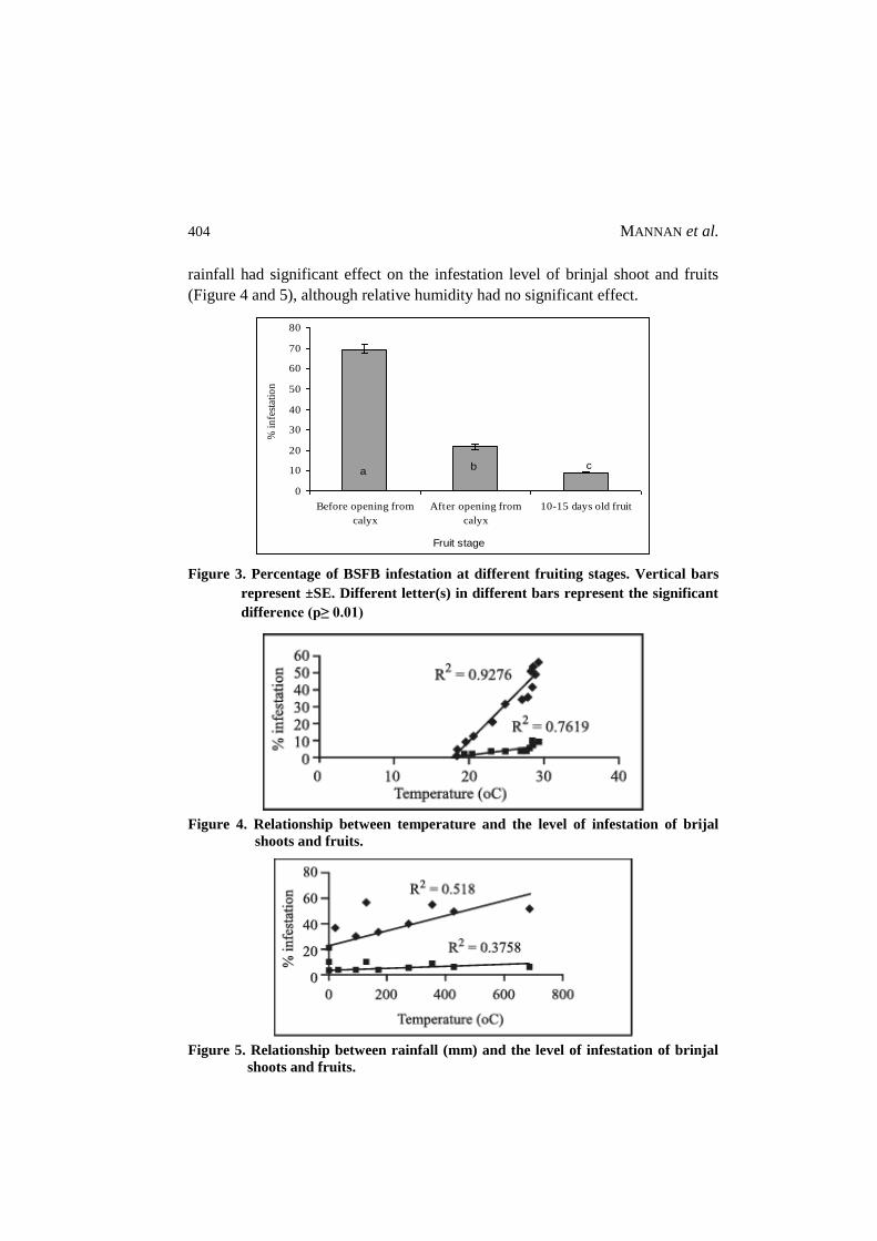
404 MANNAN et al.
rainfall had significant effect on the infestation level of brinjal shoot and fruits
(Figure 4 and 5), although relative humidity had no significant effect.
cba
0
10
20
30
40
50
60
70
80
Before opening from
calyx
After opening from
calyx
10-15 days old fruit
Fruit stage
% i
nfe
stat
ion
Figure 3. Percentage of BSFB infestation at different fruiting stages. Vertical bars
represent ±SE. Different letter(s) in different bars represent the significant
difference (p≥ 0.01)
Figure 4. Relationship between temperature and the level of infestation of brijal
shoots and fruits.
Figure 5. Relationship between rainfall (mm) and the level of infestation of brinjal
shoots and fruits.
BRINJAL SHOOT AND FRUIT BORER INFESTATION IN RELATION 405
Naik et al., (2008) reported that incidence of L. orbonalis in terms of shoot
infestation starts in February and there was no significant relationship of BSFB
infestation with the temperature, RH and rainfall. Singh et al., (2000) reported
that BSFB infestation was more serious on shoots during September to October
ranging 73.33% to 86.66% with an intensity of 2.09 borers/plant when it reached
the peak. They demonstrated a continuous decline of shoot infestation even to
zero level in the month of October. This decline was related to the initiation of
flowering and at this critical stage the borer infestation shifted from 33.33% to
66.66% in flowers and shoots which subsequently showed a greater decrease
with the advent of winter season. Mahesh and Men (2007) reported that the
infestation commenced from August with 21.2% infestation and reached its peak
during mid-October with 35.3% infestation at temperatures ranging between 21.4
and 33.00 C, relative humidity of 45-86% with 2.7 mm rain and hot sunshine.
Although it was revealed that BSFB was prevailing in the brinjal field throughout
the year, the level of infestation varied with the months and seasons of the year.
The borer infestation was found to be very low during the winter months
(December-February) which increased markedly in the summer months which was
supported by Alam et al., (2006). They reported that summer brinjal crops suffered
much greater pest damage than winter crops. Rashid et al., (2003) reported that L.
orbonalis is difficult to control in the open field during summer time. The
maximum level of borer infestation was found from June to September ranging
from 51.35 to 56.38% when the average temperature, RH and rainfall were
28.740C, 87.77% and 400.28 mm, respectively.
The trend of BSFB infestation found in present investigation has similarity with
the findings of Singh et al., (2000) and Mahesh and Men (2007) although the
level of infestation was different. The seasonal variation of the pest level is
common in many insects mostly for their poikelothermic developmental nature
i.e., the development is directly proportional to the environmental temperatures.
The variation of level of pest incidence in summer and winter may have the
relationship with the biotic factors especially some parasitoids of BSFB.
Although no attempt was made to investigate the synchronization between the
pest and parasitoids in different environmental conditions, it was assumed that
the tiny parasitoids were not able to withstand in the environmental condition
when the rainfall was high during the month of June to September.
References
Alam, S.N., M.A. Rashid, F.M.A. Rouf, R.C. Jhala, J.R. Patel, S. Satpathy, T.M.
Shivalingaswamy, S. Rai, I. Wahundeniya, A. Cork, C. Ammaranan and N.S.
Talekar. 2003. Development of an integrated pest management strategy for eggplant
fruit and shoot borer in South Asia. Technical Bulletin No. 28. AVRDC Publication
Number 03-548. AVRDC-The World Vegetable Centre, Shanhua, Taiwan. 56p.

406 MANNAN et al.
Alam, S.N., M.I. Hossain, F.M.A. Rouf, R.C. Jhala, M.G. Patel, L.K. Rath, A. Sengupta,
K. Baral, A.N. Shylesha, S. Satpathy, T.M. Shivalingaswamy, A. Cork and N.S.
Talekar. 2006. Implemntation and promotion of an IPM strategy for control of
eggplant fruit and shoot borer in South Asia. Technical Bulletin No. 36. AVRDC
Publication Number 06-672. AVRDC-The World Vegetable Centre, Shanhua,
Taiwan. 74p.
Alam, M.Z. and D.L. Sana. 1964. Biology of Leucinodes orbonalis Guenee in East Pakistan.
pp. 192-200. In: M.Z. Alam, A. Ahmed, S. Alam, M.A. Islam (eds). A Review of
Research, Division of Entomology (1947-1964). Agric. Inform. Serv. Dhaka.
Ali, M.I., A.K.M. Khorsheduzzaman, M.A. Karim and A. Ahmed. 1996. Effect of
intercropping onion, garlic and coriander with brinjal on the infestation of brinal
shoot and fruit borer. Bangladesh J. Agril. Res. 21(1): 58-63.
AVRDC. 2001. Eggplant insect pests: eggplant fruit and shoot borer. Shanhua, Taiwan.
74p.
BARI. 1991. Management of the brinjal shoot and fruit borer, Leucinodes orbonalis
Guen. pp.44-46. In: Annual Research Report. 1990-91. BARI, Gazipur, Bangladesh.
BARI. 1994. Integrated management for the brinjal shoot and fruit borer, Leucinodes
orbonalis Guen. pp.94-96. In: Annual Research Report. 1993-94. BARI, Gazipur,
Bangladesh.
Dhankar, B.S. 1988. Progress in resistance studies in eggplant (Solanum melongena L.)
against shoot and fruit borer (Leucinodes orbonalis) infestation. Trop. Pest Manage.
34:343-345.
FAO. 2000. Area and production of aubergines. Year book. 48: 136.
Ghosh, S.K. and S.K. Senapati. 2009. Seasonal fluctuation in the population of
Leucinodes orbonalis Guenee in the sub-himalayan region of West Bengal, India and
its control on eggplant (Solanum melongena). Prec. Agril. 10(5): 443-449.
Hossain, M.M., M. Shajahan, and M.A. Salam. 2002. Screening of some brinjal varieties
and lines against brinjal shoot and fruit borer, L. orbonalis Guenee. Pak. J. Biol. Sci.
5(10): 1032-1040.
Mahesh, P and U.B. Men. 2007. Seasonal incidence of Leucinodes orbonalis on brinjal.
Ann. Plant. Prot. Sci. 15(2): 498-499.
Naik, V., C. Babu, R.P. Arjuna, P.V. Krishnaya and R.V. Sriviivasa. 2008. Seasonal
incidence and management of L. orbonalis Guenee on brinjal. Ann. Plant. Prot. Sci.
16(2): 329-332.
Naresh, J.S., V. Malik, J.S. Balam and K.S. Khokar. 1986. A new record of Trathala sp.
A larval endoparasite attacking brinjal fruit borer, Leucinodes orbonalis Guen. Bull.
Entomol. New Delhi. 27(1): 74.
Patnaik, H.P. 2000. Flower and fruit infestation by brinjal shoot and fruit borer,
Leucinodes orbonalis Guenee–damage potential vs. weather. Veg. Sci. 27(1): 82-83.
Rashid, M.A., S.N. Alam, F.M.A. Rouf and N.S. Talekar. 2003. Socio economic
parameters of brinjal pest control in Jessore district of Bangladesh. Technical

BRINJAL SHOOT AND FRUIT BORER INFESTATION IN RELATION 407
Bulletin No. 29. Shanbua, Taiwan. AVRDC-The world vegetable centre. AVRDC
publication No. 03-556. 29p.
Regupathy, A., N.J. Armes, G. Asoken, D.R. Jadhav, R.D. Soundarajan and D.A. Russell.
1997. Best method for insecticide resistance management of Helicoverpa armigera.
In: International Conference on Integrated Approach to Combating Resistance. A.L.
Devonshine (ed.), April 14-16, 1997. IACR, Rothamsted, Harpendle, UK. 116p.
Sharma, A.K. and R.C. Chhibber. 1999. Effect of exposure periods and insecticides on
Leucinodes orbonalis in brinjal. Indian J. Entomol. 61(3): 242-251.
Singh, S.V., K.S. Singh and Y.P. Malik. 2000. Seasonal abundance and economic losses
of shoot and fruit borer, Leucinodes orbonalis on brinjal. Indian J. Entomol. 62(3):
247-252.
Singh, N.P., N.S.A. Thakur, A.N. Shyclesha and S. Biswas. 2005. Implementation and
Promotion of IPM technology for the control of eggplant shoot and fruit borer
(Leucinodes orbonalis Guenee) in Meghalaya and Tripura. Publication No.-17.
AVRDC, Post Box: 42, Sanghua, Taiwan 741.
Tewari, G. and H.R. Sardana. 1990. An unusual heavy parasitization of brinjal shoot
and fruit borer, Leucinodes orbonalis Guenee by a new braconid parasite.
Indian J. Entomol. 52(2):338-341.

408 MANNAN et al.

ISSN 0258-7122
Bangladesh J. Agril. Res. 40(3): 409-420, September 2015
PROFITABILITY OF BETEL LEAF (Piper betle L.) CULTIVATION IN
SOME SELECTED SITES OF BANGLADESH
Q. M. S. ISLAM1, M. A. MATIN
2, M. A. RASHID
3
M. S. HOQ4 AND MONIRUZZAMAN
5
Abstract
The study was conducted in four betel leaf growing areas, namely Barisal,
Chittagong, Rajshahi and Kustia district during 2013-14 to assess the cultivation
practices, physical productivity, profitability, and to explore the constraints to
betel leaf cultivation. The study has been designed to investigate the economics
of betel leaf production considering intensive cultivated areas for recent
information in Bangladesh. From each district, two upazilas were selected
considering the concentration of betel leaf growers and easy access. Also from
each upazila, two blocks and from each block 20 farmers were selected with the
consultation of Upazila Agriculture Officer and Sub Assistant Agriculture
Officer. The study revealed that betel leaf cultivation was profitable in the study
areas, although BCR in the first and second years was below one which was due
to high initial cost. The highest yield and gross return of betel leaf cultivation
were in the fifth year. The benefit cost ratio was found highest in 6-10 year
followed by 5th
and 11-15 year. The benefit cost ratio at 12%, 15% and 20% rate
of interest were 1.27, 1.25 and 1.21 respectively. Internal rate of return (IRR)
was calculated 62% in current situation, IRR 37% was found by 10% decrease
of return and 39% by 10% increase of cost. The problems like leaf rot disease,
high price of boroj materials, low price of betel leaf, high price of oilcake, etc.
were facing by the betel leaf farmers.
Keywords: Betel leaf, BCR, IRR, NPV, Constraints.
Introduction
Betel leaf (Piper betle L.), locally known as Paan, is a masticatory having
important socio-cultural and ceremonial uses in South and Southeast Asia,
significant medicinal properties and nutritional values. The vine is native to
Southeast Asia including Bangladesh which is thought to be one of the cradles of
earliest agriculture. The betel leaf plant is an evergreen and perennial creeper,
with glossy heart-shaped leaves and white catkin. It is a native of central and
eastern Malaysia, which spread at a very early date throughout tropical Asia and
later to Madagascar and East Africa (www.efymag.com/ admin/issuepdf/
Betel%20Leaf_April-12.pdf).
Betel leaf a kind of pepper used in wrapping the pellets of betel nut and lime, is
commonly chewed in the orient. Betel leaf is an important cash crop in our
1-3Principal Scientific Officer,
4Scientific Officer,
5Senior Scientific Officer, Agricultural
Economics Division, BARI, Joydebpur, Gazipur, Bangladesh.

410 ISLAM et al.
country and is considered to be one of the ingredients for social entertainment. It
has also a sharp taste and good smell, improves taste and appetite, tonic to the
brain heart, liver, strengthens the teeth and clears the throat.
Table 1: Area and production of betel leaf in Bangladesh
Year Area (ha) Production (tons) Yield (t/ha)
1995-96 13943 71910 5.16
1996-97 14595 77035 5.28
1997-98 14832 79080 5.33
1998-99 13820 73525 5.32
1999-00 15063 78780 5.23
2000-01 15346 82260 5.36
2001-02 14696 80540 5.48
2002-03 15472 83830 5.42
2003-04 16480 93425 5.67
2004-05 16771 93820 5.59
2005-06 16275 97415 5.99
2006-07 16536 101240 6.12
2007-08 17346 97947 5.65
2008-09 17643 105448 5.98
2009-10 17871 91681 5.13
2010-11 18247 105953 5.81
Mean 15934 88368 5.53
CV (%) 8.84 12.81 5.63
Growth rate (%) 1.80 2.50 0.70
Source: BBS, 2011
In 2010-11, the total betel leaf area was 18,247 ha (31% higher than the area in
1995-96) with a production of 1,05,953 tons (47% higher than the production in
1995-96) in Bangladesh. The area of this crop has been increasing at an
increasing rate (1.8%) over the years (Table 1). Betel leaf has become a
promising commodity with an increasing trend of export every year
(Anonymous, 1984).
The country may earn a huge amount of foreign currency every year by exporting
betel leaf in different countries. However, data and information regarding betel
leaf production and the status of local and international marketing system are
scarce in the country. A very few studies were conducted (Ahmed, 1985; Islam
and Elias 1991 and Moniruzzaman, et. al 2008) regarding the profitability and

PROFITABILITY OF BETEL LEAF CULTIVATION IN SOME SELECTED 411
constraints to higher production as well as export potentiality of betel leaf
production in Bangladesh. Earlier studies were conducted very limited areas and
back dated. Thus, the present study has been designed to investigate the
economics of betel leaf cultivation considering intensive cultivated areas. This
study provides useful information to the policy makers to make policy guidelines
for enhancing its production as well as its overall development in the near future.
Therefore, the present study was undertaken with the following specific
objectives:
1. To know the agronomic practices of betel leaf at growers level.
2. To determine the cost and return of betel leaf cultivation.
3. To estimate physical productivity and returns to investment in betel leaf
cultivation, and
4. To find out the constraints of betel leaf cultivation at farm level.
Methodology
Study area and sampling technique: Multi-stage sampling technique was
followed in this study. Four betel leaf growing districts namely Barisal,
Chittagong, Rajshahi and Kustia were purposively selected. Again from each
district, two upazilas were selected considering the concentration of betel leaf
growers and easy access. Also from each upazila, two blocks were selected with
the consultation of Upazila Agriculture Officer. A list of betel leaf growers from
the selected blocks was prepared with the help of DAE personnel. Thus a total of
4×2×2×16 = 256 samples were randomly selected for the interview.
Data collection and period of study: Experienced field investigators with the
direct supervision of the researchers collected data and information using a pre-
tested interview schedule. Data were collected during the period of November to
April, 2013-14.
Analytical technique: (a) Tabular method of analysis using descriptive statistics
like average, percentage, ratio etc. was followed in presenting the results of the
study. Data were categorized according to the age of betel leaf boroj. The age of
the boroj were classified like 1st year, 2
nd year, 3
rd year, 4
th year, 5
th year, (6-10)
th
year, (11-15) th
year and (16 and above) th
year. Because both cost of production
and yield were vary year to year. Collected data were edited, summarized,
tabulated and analyzed to fulfill the objectives of the study. (b) To measure the
return to investment of betel leaf cultivating project appraisal technique. For
measuring capital productivity, costs and returns were discounted at 12 %, 15%
and 20% rate of interest. The Benefit cost ratio (BCR), Net present value(NPV)
and Internal rate of return(IRR) in betel leaf cultivation were calculated with the
help of following formula.
412 ISLAM et al.
Net present Value =
nt
tt
tt
i
CB
1 )1(
Benefit cost ratio =
t
tnt
t
nt
tt
t
i
C
t
B
)1(
)1(
1
1
Internal
Rate of
Return
(IRR) =
Lower
discount
rate +
Difference
between
the
discount
rates
×
Present worth of incremental net
benefit stream (cash flow) at the
lower discount rate
Sum of the present worth of the
incremental net benefit streams
(cash flows) at the two discount
rates, signs ignored
Where, Bt = Total benefit (Tk/ha) in tth year
Ct = Total cost (Tk/ha) in tth year
t = Number of year
i = interest (discount) rate.
Results and Discussion
1. Agronomic practices of betel leaf cultivation
Respondent farmers did not plough their land for betel leaf cultivation. They
prepared their land by spading. The most appropriate planting time of the betel
leaf is at the end of the rainy season mostly from July to October by the farmers.
The respondent farmers used betel leaf vine as seed which was mostly local
variety. Within local varieties, farmers mainly cultivated Mohanali, Chailtagota
and Cherifuli in Barisal, Mithapaan, Dholshi in Chittagong, Banglapaan,
Mithapaan in Rajshahi and Mistipaan, Khilipaan in Kustia district. Modern
varieties of betel leaf are not available in the study areas. The average number of
betel leaf seed (vine) was found to be 123845 to 172841 numbers per hectare.
The average plant to plant distance was found 15.24-20.32cm and line to line
spacing of betel leaf vine were found to be 45.72-55.88 cm in Barisal and
Chittagong. But in Rajshahi and Kustia the line to line spacing were found
81.28-91.44 cm. The average number of earthing up, application of oilcake,
weeding, spraying and irrigation were 1.96, 4.23, 1.86, 5.82 and 6.02 respectively
(Table 2). In Table-1, the average number of irrigation was 6.02. But in
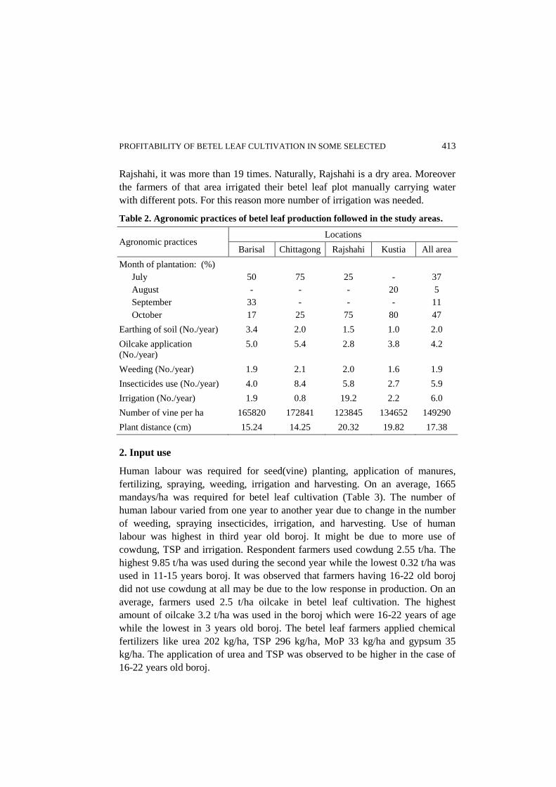
PROFITABILITY OF BETEL LEAF CULTIVATION IN SOME SELECTED 413
Rajshahi, it was more than 19 times. Naturally, Rajshahi is a dry area. Moreover
the farmers of that area irrigated their betel leaf plot manually carrying water
with different pots. For this reason more number of irrigation was needed.
Table 2. Agronomic practices of betel leaf production followed in the study areas.
Agronomic practices Locations
Barisal Chittagong Rajshahi Kustia All area
Month of plantation: (%)
July
August
September
October
50
-
33
17
75
-
-
25
25
-
-
75
-
20
-
80
37
5
11
47
Earthing of soil (No./year) 3.4 2.0 1.5 1.0 2.0
Oilcake application
(No./year)
5.0 5.4 2.8 3.8 4.2
Weeding (No./year) 1.9 2.1 2.0 1.6 1.9
Insecticides use (No./year) 4.0 8.4 5.8 2.7 5.9
Irrigation (No./year) 1.9 0.8 19.2 2.2 6.0
Number of vine per ha 165820 172841 123845 134652 149290
Plant distance (cm) 15.24 14.25 20.32 19.82 17.38
2. Input use
Human labour was required for seed(vine) planting, application of manures,
fertilizing, spraying, weeding, irrigation and harvesting. On an average, 1665
mandays/ha was required for betel leaf cultivation (Table 3). The number of
human labour varied from one year to another year due to change in the number
of weeding, spraying insecticides, irrigation, and harvesting. Use of human
labour was highest in third year old boroj. It might be due to more use of
cowdung, TSP and irrigation. Respondent farmers used cowdung 2.55 t/ha. The
highest 9.85 t/ha was used during the second year while the lowest 0.32 t/ha was
used in 11-15 years boroj. It was observed that farmers having 16-22 old boroj
did not use cowdung at all may be due to the low response in production. On an
average, farmers used 2.5 t/ha oilcake in betel leaf cultivation. The highest
amount of oilcake 3.2 t/ha was used in the boroj which were 16-22 years of age
while the lowest in 3 years old boroj. The betel leaf farmers applied chemical
fertilizers like urea 202 kg/ha, TSP 296 kg/ha, MoP 33 kg/ha and gypsum 35
kg/ha. The application of urea and TSP was observed to be higher in the case of
16-22 years old boroj.

414 ISLAM et al.
Table 3. Per hectare input used for betel leaf cultivation in the study areas.
Parameters
Period of cultivation (Year)
1st 2
nd 3
rd 4
th 5
th 6-10 11-15 16 -22 All
Observations n=19 n=23 n=48 n=44 n=37 n=55 n=30 n=11 n=256
Human labour
(mandays)
1385 1509 1694 1619 1693 1598 1522 1491 1665
Own 662 655 790 666 718 667 605 679 718
Higher 723 854 904 953 975 931 917 812 947
Seed(Vine) 123748
Cowdung(ton) 5.5 9.9 3.7 2.2 4.9 3.2 3.8 - 2.5
Oilcake(ton) 2.4 2.5 2.3 2.3 2.3 2.6 2.5 3.2 2.5
Fertilizer
(kg):
Urea 117 207 165 202 213 211 190 248 202
TSP 386 321 343 276 237 208 239 452 296
MP 21 56 37 24 22 20 63 15 33
Gypsum 33 87 53 110 36 35 9 45 55
Others* 26 20 5 17 12 12 - 2 12
* Others indicate DAP, Zn, Boron, etc.
3. Cost of production
The cost of production included human labour, boroj making materials, seed
(vine), manures, fertilizers, pesticides, irrigation, insecticides, etc. Rental value of
land was treated as fixed cost and was included in the total costs. Seed (vine) cost
was needed only for the first year. The highest cost (Tk 1088333/ha) was
incurred in the first year due to initial investment on seed (vine) and boroj
making materials. The lowest cost (Tk 885035/ha) was observed for the boroj
aged ranged from 11-15 years (Table 4). Among the cost items of betel leaf
cultivation human labour incurred the highest cost (50%) followed by boroj
materials cost (26%).
4. Return
For estimating the yield of betel leaf, data were collected from the survey plot on
the basis of local unit like bira, Sali, gadi, kuri, pon etc. After that yield data were
converted into ton per hectare on the basis of average weight of betel leaf. On an
average, the weight of 265 number of betel leaf is one kilogram (Moniruzzaman,
2008). On review of Table 3, it is observed that the yield started increasing
during 2nd
to 5th year and declined form thereafter. Among the betel leaf boroj,
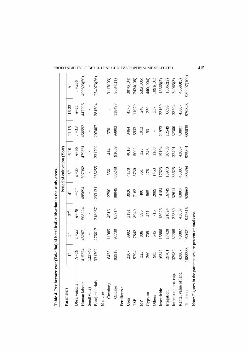
PROFITABILITY OF BETEL LEAF CULTIVATION IN SOME SELECTED 415
Ta
ble
4.
Per
hec
tare
co
st (
Tak
a/h
a)
of
bet
el l
eaf
cult
iva
tion
in
th
e st
ud
y a
rea
s.
Par
amet
ers
Per
iod o
f cu
ltiv
ati
on (
Yea
r)
1st
2nd
3rd
4
th
5th
6
-10
1
1-1
5
16
-22
All
Ob
serv
ati
on
s N
=1
9
n=
23
n=
48
n=
44
n=
37
n=
55
n=
19
n=
11
n=
25
6
Hu
man
lab
our
4
15
37
4
45
267
1
50
822
4
48
569
4
50
796
2
47
933
1
45
659
2
44
729
6
49
939
3(5
0)
See
d(V
ine)
1
23
74
8
- -
- -
- -
- -
Bo
roj
mat
eria
ls
33
179
2
27
661
7
21
806
7
23
313
1
26
525
5
23
179
2
20
740
7
28
150
4
25
497
3(2
6)
Man
ure
s:
C
ow
dun
g
64
35
11
985
4
51
6
27
90
55
6
41
4
57
0
- 3
11
7(.
03)
O
ilca
ke
92
918
97
730
8
57
14
88
049
86
248
91
669
99
903
11
849
7
95
841
(1)
Fer
tili
zers
:
Ure
a 2
30
7
39
92
31
91
39
20
41
78
40
13
34
64
45
70
38
70(.
04)
TS
P
97
94
78
42
89
49
71
63
57
30
50
92
59
33
11
070
74
34(.
08)
MP
3
23
88
6
59
5
40
0
36
1
32
8
10
13
24
0
53
5(.
00
5)
Gyp
sum
2
60
70
9
47
1
86
5
27
8
24
6
93
35
9
44
0(.
00
4)
Oth
ers
98
5
54
5
71
6
20
89
14
53
11
68
- 3
37
10
91(.
01)
Inse
ctic
ide
1
63
42
15
886
1
89
26
14
184
17
623
19
194
21
973
23
169
18
868
(2)
Irri
gat
ion
19
701
17
428
2
16
24
16
749
18
973
16
759
12
549
66
99
18
062
(2)
Inte
rest
on o
pt.
cap
. 3
29
82
32
208
3
23
30
32
611
33
625
32
491
32
300
33
294
34
065
(3)
Ren
tal
val
ue
of
land
4
38
07
43
807
4
38
07
43
807
43
807
43
807
43
807
43
807
45
689
(5)
To
tal
cost
1
08
83
33
95
032
1
94
261
6
92
866
3
98
549
4
92
589
1
88
503
5
97
084
3
98
929
7(1
00
)
No
te:
Fig
ure
s in
the
par
enth
eses
are
per
cent
of
tota
l co
st.

416 ISLAM et al.
Ta
ble
5
. P
rofi
tab
ilit
y o
f b
etel
lea
f cu
ltiv
ati
on
in
th
e st
ud
y a
rea
s.
Item
P
erio
d o
f cu
ltiv
ati
on (
Yea
r)
All
1st
2nd
3rd
4
th
5th
6
-10
1
1-1
5
16
-22
Ob
serv
ati
on
s n
=1
9
n=
23
n=
48
n=
44
n=
37
n=
55
n=
19
n=
11
n=
25
6
Yie
ld(t
/ha)
5
.80
6.0
3
7.0
5
7.8
0
9.5
0
9.3
1
7.8
4
6.9
6
8.2
3
T.
var
iab
le c
ost
(T
k/h
a)
50
415
3
49
231
7
49
419
3
49
848
5
51
398
0
49
665
2
49
373
2
50
892
7
52
070
3
Gro
ss r
eturn
(T
k/h
a)
70
332
0
90
171
1
10
579
55
12
931
60
15
386
51
14
507
96
13
192
87
11
585
79
12
989
85
Gro
ss m
argin
(Tk/h
a)
28
916
6
40
939
3
56
376
3
79
467
6
10
246
72
95
414
5
82
555
5
64
965
2
77
828
2
Net
ret
urn
(Tk/h
a)
51
649
38
480
8
55
887
4
85
975
0
11
536
20
91
351
1
53
078
5
11
528
9
72
111
6
BC
R o
n
full
co
st b
asis
0
.73
0.9
5
1.1
2
1.3
9
1.5
6
1.5
7
1.4
9
1.1
9
1.3
8
BC
R o
n
cash
co
st b
asis
0
.93
1.1
3
1.3
0
1.5
4
1.6
2
1.6
3
1.5
6
1.2
5
1.1
0
Ret
urn
s to
lab
our
(Tk/m
an
-day)
87
26
8
36
8
52
5
62
7
62
9
58
5
42
6
48
6
Ta
ble
6
. C
ost
ben
efit
an
aly
sis
of
bet
el l
eaf
pro
du
ctio
n i
n t
he
stu
dy
are
as.
Yea
r o
f
bo
roj
Co
st
(Tk/h
a)
Dis
cou
nt
fact
or
(DF
) D
isco
unte
d c
ost
at
Gro
ss r
eturn
(T
k/h
a)
Dis
cou
nte
d b
enef
it a
t
12
%
15
%
20
%
12
%
15
%
20
%
1
2%
1
5%
2
0%
1
10
883
33
0.8
9
0.8
7
0.8
3
97
172
6
94
637
7
90
694
4
79
332
0
70
832
1
68
984
3
66
110
0
2
95
032
1
0.8
0
0.7
6
0.6
9
75
759
0
71
857
9
65
994
5
90
171
1
71
883
8
68
182
3
62
618
8
3
94
261
6
0.7
1
0.6
6
0.5
8
67
093
5
61
978
5
54
549
5
10
579
55
75
303
2
69
562
3
61
224
3
4
92
866
3
0.6
4
0.5
7
0.4
8
59
018
2
53
096
6
44
785
1
12
931
60
82
182
7
73
936
9
62
363
1
5
98
549
4
0.5
7
0.5
0
0.4
0
55
919
6
48
996
5
39
604
8
15
386
51
87
307
2
76
498
2
61
835
0
6-1
0
92
589
1
0.5
1
0.4
3
0.3
3
46
908
5
40
028
8
31
007
9
14
507
96
73
501
9
62
721
9
48
586
9
11
-15
88
503
5
0.2
9
0.2
1
0.1
3
25
442
6
19
023
2
11
911
5
13
192
87
37
926
3
28
357
2
17
756
0
16
-22
97
084
3
0.1
6
0.1
1
0.0
5
15
837
1
10
375
3
52
513
11
585
8
18
899
12
381
62
67
To
tal
59
250
83
52
044
26
42
874
52
7
54
29
75
65
056
48
52
008
13
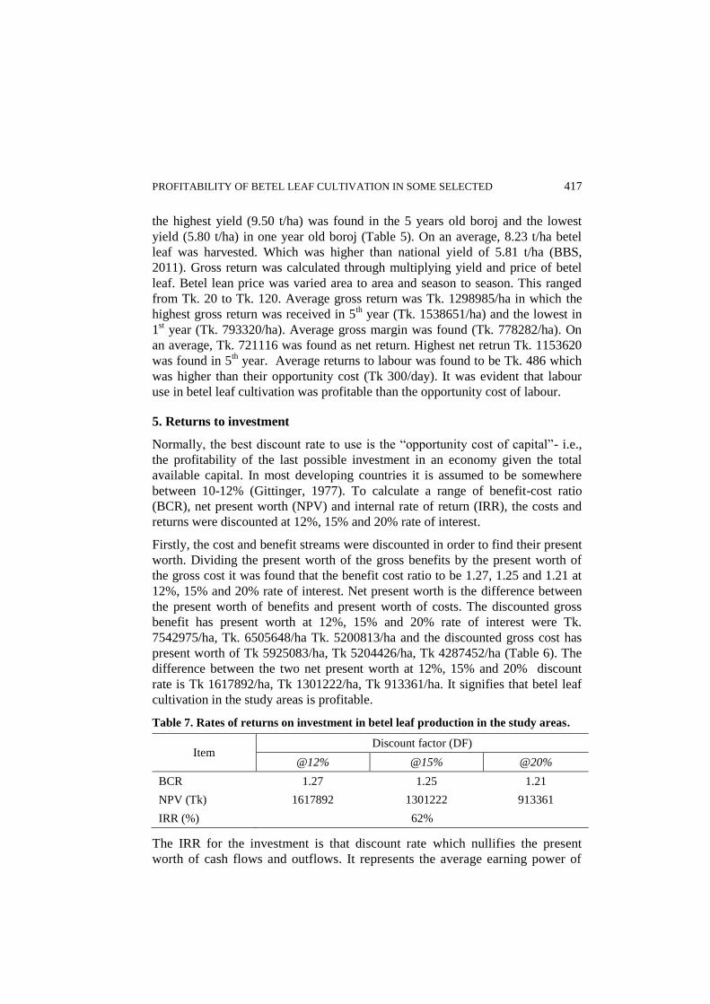
PROFITABILITY OF BETEL LEAF CULTIVATION IN SOME SELECTED 417
the highest yield (9.50 t/ha) was found in the 5 years old boroj and the lowest
yield (5.80 t/ha) in one year old boroj (Table 5). On an average, 8.23 t/ha betel
leaf was harvested. Which was higher than national yield of 5.81 t/ha (BBS,
2011). Gross return was calculated through multiplying yield and price of betel
leaf. Betel lean price was varied area to area and season to season. This ranged
from Tk. 20 to Tk. 120. Average gross return was Tk. 1298985/ha in which the
highest gross return was received in 5th year (Tk. 1538651/ha) and the lowest in
1st year (Tk. 793320/ha). Average gross margin was found (Tk. 778282/ha). On
an average, Tk. 721116 was found as net return. Highest net retrun Tk. 1153620
was found in 5th year. Average returns to labour was found to be Tk. 486 which
was higher than their opportunity cost (Tk 300/day). It was evident that labour
use in betel leaf cultivation was profitable than the opportunity cost of labour.
5. Returns to investment
Normally, the best discount rate to use is the “opportunity cost of capital”- i.e.,
the profitability of the last possible investment in an economy given the total
available capital. In most developing countries it is assumed to be somewhere
between 10-12% (Gittinger, 1977). To calculate a range of benefit-cost ratio
(BCR), net present worth (NPV) and internal rate of return (IRR), the costs and
returns were discounted at 12%, 15% and 20% rate of interest.
Firstly, the cost and benefit streams were discounted in order to find their present
worth. Dividing the present worth of the gross benefits by the present worth of
the gross cost it was found that the benefit cost ratio to be 1.27, 1.25 and 1.21 at
12%, 15% and 20% rate of interest. Net present worth is the difference between
the present worth of benefits and present worth of costs. The discounted gross
benefit has present worth at 12%, 15% and 20% rate of interest were Tk.
7542975/ha, Tk. 6505648/ha Tk. 5200813/ha and the discounted gross cost has
present worth of Tk 5925083/ha, Tk 5204426/ha, Tk 4287452/ha (Table 6). The
difference between the two net present worth at 12%, 15% and 20% discount
rate is Tk 1617892/ha, Tk 1301222/ha, Tk 913361/ha. It signifies that betel leaf
cultivation in the study areas is profitable.
Table 7. Rates of returns on investment in betel leaf production in the study areas.
Item Discount factor (DF)
@12% @15% @20%
BCR 1.27 1.25 1.21
NPV (Tk) 1617892 1301222 913361
IRR (%) 62%
The IRR for the investment is that discount rate which nullifies the present
worth of cash flows and outflows. It represents the average earning power of

418 ISLAM et al.
the money used in the project over the project life. In betel leaf project, IRR is
62%. It is acceptable, because it is much higher than the opportunity cost of
capital (Table 8).
Sensitivity Analysis
To make a valid generalization it was necessary to conduct sensitivity analysis.
This table has been reworked separately to see what happens on the profitability
of betel leaf under varying conditions. The cost of betel leaf cultivation was
considered constant, while benefit decreases at the rate of 10% or if benefit of the
betel leaf cultivation remains the same but all costs increase at the rate of 10%
then what would be the outcome.
Table 8. Result of sensitivity analysis of betel leaf cultivation in the study areas.
Situation Discount measures
BCR at 12% NPV at 12% IRR (%)
Base parameter 1.27 Tk. 1617892 62
Decrease of return:
10% 1.04 Tk. 271086 37
Increase of gross cost:
10% 1.16 Tk. 102583 39
The results of sensitivity analysis considering the above mentioned situation are
presented in Table 8. It was revealed from the table 7 that BCR of betel leaf is
greater than one, NPV is positive at 12% discount rate and IRR is also higher
than the opportunity cost of capital. This implies that if the returns decrease at
10% the cost of betel leaf remains unchanged investment in betel leaf is
profitable from the point of view of the owner. Again, BCR of the betel leaf is
greater than one. NPV is positive and IRR is higher than the opportunity cost of
capital, if gross cost increases at 10% the returns remain same. This means that
the owner of betel leaf boroj can also make profit if all costs slightly increase in
near future. The result of the study indicates that the owners of betel leaf boroj
can earn profits under changing situation.
Constraints
Every farmer opined one or more than one problems (Table 9). Leaf rot disease
was a common problem in the study areas. About 79% farmers opined that it is a
serious problem for betel leaf cultivation. High price of boroj materials was
another problem reported by the farmers. Many farmers reported that vine died at
the end of the vine and sometimes 2-3 ft upper was a common problem which
hampered the betel leaf production. About 45% farmers faced the problem of
capital shortage during betel leaf cultivation. Cumbersome procedure of

PROFITABILITY OF BETEL LEAF CULTIVATION IN SOME SELECTED 419
institutional credit was also a common problem in the study area. Price of betel
leaf is very low during rainy season i.e. during the months of June to August.
Regarding seed (vine), respondents had mentioned the problem of non-
availability of quality seed. They did not know about the modern varieties of
betel leaf. Though BARI released two betel leaf varieties but these were not
reached to the farmer’s field. Farmers used much quantity of oilcake in their
boroj. Some of the responded opined that price of oilcake was very high. For this
reason some of the farmers were unable to apply oilcake according to their
desired level. Huge number of labour is required for betel leaf cultivation. About
17% farmers faced the problem of non-availability of labour. Non-availability of
irrigation water was also a problem opined by 13% respondent. It is essential to
irrigate the betel leaf boroj during dry period. High price of insecticides was also
mentioned by 7% farmers. Besides, some farmers mentioned that insect
infestation, excess cold, lack of transportation facilities were also the constraints
of betel leaf cultivation.
Table 9. Constraints faced by the respondent betel leaf growers in the study areas.
Constraints % of responses (n=256)
1. Infection of leaf rot disease 79
2. High price of boroj materials 56
3. Seed (vine) died 52
4. Lack of capital 45
5. Low price of betel leaf 41
6. Non-availability of modern varieties 32
7. High price of oilcake 21
8. Non-availability of labour 17
9. Non-availability of irrigation water 13
10. High price of insecticides 7
11. Others* 27
* Others indicate insect infestation, excess cold, lack of transport facilities etc.
Conclusion and Recommendation
The study has estimated the agronomic practices, profitability, returns to
investment of betel leaf cultivation and constraints to its cultivation at farm level.
The benefit cost ratio, net present worth and internal rate of return indicate that
betel leaf cultivation is profitable. Sensitivity analysis also indicates that the
owners of betel leaf boroj can earn profit under changing situation. Although
betel leaf cultivation is profitable, but farmers faced various problems such as
infection of leaf rot disease, high price of boroj materials, vine died, lack of
420 ISLAM et al.
capital, low price of betel leaf, high price of oilcake, non-availability of modern
variety, labour scarcity, and lack of irrigation water.
For controlling leaf rot disease of betel leaf, pathologist may conduct research on
this aspect. It is also imperative to carry out more research on developing high
yielding varieties of betel leaf and develop appropriate production technologies
for maximizing the yield as well as income and minimizing the cost. Extension
works with publicity need to be strengthened to popularize the modern varieties
of betel leaf in order to expand its cultivation area.
References
Ahmed, A.U. 1985 Disease Problems of Betel Leaf Vine in Kushtia Area, Plant
Pathology Division, BARI, Joydebpur, Gazipur.
Anonymous, 1984. Export form Bangladesh during the fiscal year 1970-71 to 1983-84,
Export promotion Bureau, Motigheel commercials Area, Dhaka, Bangldesh.
Bangladesh Bureau of Statistics, 2011. Yearbook of Agricultural Statistics of Bangldesh.
Statistical Division, Ministry of Planning. GOB. P. 76.
Gittiner, J.P. 1977. Economic Analysis of Agricultural Project. A World Bank
Publication.]
Islam, M.N and S.M. Elias (1991), Production and Marketing of Betel leaf in selected
areas of Bangladesh, Research Report No. 16, Agricultural Economics Division,
BARI, Joydebpur, Gazipur.
Moniruzzaman, M.S. Rahman, M.A Hossain and Q.M. Alam(2008). Betel Leaf
Production and Its Market Potential on National and International Market. Annual
Research Report , Agricultural Economics Division, BARI, Joydebpur, Gazipur.

ISSN 0258-7122
Bangladesh J. Agril. Res. 40(3): 421-433, September 2015
GENETIC DIVERGENCE IN Brassica rapa L.
S. NAZNIN1, M. A. KAWOCHAR
2, S. SULTANA
3
N. ZEBA4
AND S. R. BHUIYAN5
Abstract
Different multivariate analysis techniques were used to classify 33 Brassica
rapa L. genotypes. The genotypes were grouped into five clusters. Cluster I
contained the maximum number of genotypes. Cluster III earned the highest
cluster mean value for number of primary branches/plant, number of secondary
branches/plant, number of siliquae/plant and seed yield/plant. Therefore, more
emphasis can be given on cluster III for selecting genotypes as parents for the
hybridization program. The highest intra-cluster distance (3.822) was found in
cluster I and the lowest (0.000) in cluster V. The highest inter-cluster distance
(15.705) was observed between clusters III and V showing wide diversity
among the groups. Principal component analysis (PCA) showed that the first
three principal components accounted for 99.38 % of the total variation
observed. Analysis of the factor loading of the component character indicated
that the characters number of siliquae/plant, plant height and days to maturity
were found responsible for genetic divergence. The role of number of
siliquae/plant
in both the vectors was important components for genetic
divergence in these materials. Among the possible 528 combinations, the highest
inter-genotypic distance (1.5975) was observed between G-27 (BARI sarisha-9
x BARI sarisha-6 S-62) and G-31 (BARI sarisha-15). Considering group and
inter-genotypic distance, cluster mean, contribution of different characters
towards the total divergence and other agronomic performance the genotypes G-
19 (BARI sarisha-6 x TORI-7 S-48), G-20 (F6 x BARI sarisha-9 S-52), G-27
and G-30 (BARI sarisha-6 x TORI-7 S-37) from cluster III; G-26 (F6 x BARI
sarisha-9 S-15) and G-31 from cluster IV and G-33 (BARI sarisha-6) from
cluster V would be considered as better parents for future hybridization
program.
Keywords: Genetic diversity, principal component analysis, principal coordinate
analysis, cluster analysis, Brassica rapa L.
Introduction
Brassica rapa L. commonly known as field mustard or turnip mustard belonging
to the family Brassicaceae. The seeds of Brassica rapa L. contain 42% oil and
25% protein (Khaleque, 1985). It also serves as important source of raw material
1-3Scientific Officer (Plant Breeding), Tuber Crops Research Centre, Bangladesh
Agricultural Research Institute, Gazipur-1701, 4&5
Professor, Department of Genetics and
Plant Breeding, Sher-e-Bangla Agricultural University, Dhaka-1207, Bangladesh.

422 NAZNIN et al.
for industrial use such as in making soaps, paints, hair oils, lubricants, textile
auxiliaries, pharmaceuticals and so on. It is the third most important oil crop in
the world accounting for over 16% of the world’s edible oil supply (Anonymous,
2005). It also plays an important role to the total edible oil production in
Bangladesh. Among the oil crops grown in Bangladesh Brassica rapa L.
occupies the first position in respect of area and production. During 2010-11,
about 0.252 million hectare of land was under Brassica rapa L. and mustard
cultivation where produced about 0.246 million tons of seed, and national
average yield was 0.977 ton/ha in this country. Total annual edible oil production
was about 0.833 million tons which is very low against the requirement of
Bangladesh. Bangladesh imported 89.97 thousand tons of edible oil of rapeseed in
the year of 2010-11 to meet up the annul requirement, which costs Tk.3718.457
million (BBS, 2011). The main reasons behind these are the use of low yielding
local indigenous cultivars, low management practices and reduction of
cultivation area. The area for rapeseed and mustard was reduced from 0.3177
million hectare in 2000-01 to 0.2340 million hectare in 2008-09. There was
26.32% reduction in area for this crop (Bhuiyan, 2012). For increasing the
production of Brassica rapa L., expansion of cultivated area and unit area
production are needed. There is a limited scope for horizontal expansion of its
cultivation. Thus, to increase the production of Brassica rapa L., production per
unit area must be increased. Moreover the crop should fit in the cropping pattern.
Therefore, high yielding and short duration Brassica rapa L. varieties should be
developed to fit into the existing cropping pattern (T-amon-mustard-Boro).
Genetic diversity refers to sum total of genetic variations found in a species or
population. Existence of genetic diversity is very essential to meet the present
and future crop breeding challenges. It is a prerequisite for the development of
improved cultivars with wider adaptability and broad genetic base. It can be
estimated through biometrical procedures such as Mahalanobis's D2-statistic and
is possible to choose genetically diverse parents. Diversity analysis greatly helps
the breeder in identification and proper choice of parents for specific breeding
objectives. The selection of potential varieties in a breeding program is based on
the knowledge of genetic diversity amongst them. To realize heterosis,
genetically divergent parents are generally considered to be useful. In such
crosses more variability could be expected in the resulting segregating progenies
(Joseph et al., 1999). Precise information about the extent of genetic divergence
on characters used for discrimination among the population is crucial in any crop
improvement program, because selection of plants based on genetic divergence
has become successful in several crops (Ananda and Rawat 1984; De et al.,
1988). Therefore the present study was undertaken to collect information on
GENETIC DIVERGENCE IN Brassica rapa L. 423
genetic divergence in the genotypes and selection of suitable diverse parents for
the utilization in future hybridization program.
Materials and Method
The experiment was conducted at the field of Sher-e-Bangla Agricultural
University farm, Dhaka, during rabi, 2011-12. Thirty-three genotypes were used
in this experiment where three of them were used as checks. Among the
genotypes, thirty were selected from F9 segregating generation on the basis of
their variation in different traits. The experiment was laid out in a Randomized
Complete Block Design with three replications. Each plot was 3m long with two
rows. The distance of 10 cm between plants, 30cm between rows and 1m
between blocks were maintained. Seeds were sown in lines in the experimental
plots on 29th October 2011. Recommended doses of fertilizers and standard
cultural practices were applied for raising healthy crops. Data were recorded on
randomly ten selected plants from each plot and plants were selected from middle
to avoid border effect of the plot. Data were recorded on days to maturity, plant
height (cm), number of primary branches/plant, number of secondary/branches
plant, number of siliquae/plant, siliqua length (cm), number of seeds/siliqua,
1000 seed weight (g) and seed yield/plant (g). All the collected data of the study
were subjected to statistical analysis. Multivariate analysis viz., Principal
Component Analysis (PCA), Principal Coordinate Analysis (PCO), Canonical
Variate Analysis (CVA) and Cluster Analysis were done by using GENSTAT 5
Release 4.1 (PC/Windos NT) software program (Copyright, 1997, Lawes
Agricultural Trust, Rothamasted Experimental Station, UK).
Using standardized data, numerical measures of likeness/similarity were
computed and distance matrix was constructed using Euclidean Distance
Coefficients. Clustering by UPGMA (Unweighted Pair Group of Arithmetic
Mean) method was executed (Siopongco et al., 1999). Dendogram was
constructed by using the SPSS.16 software. PCO is equivalent to PCA but it is
used in calculating inter genotypic distance and intra cluster distance for all
possible combination. When the clusters were formed, the average intra-cluster
distances for each cluster was calculated by taking possible D2
values within the
member of a cluster obtained from the PCO. CVA was performed to get the inter
cluster distances. Principal Components were computed from the correlation
matrix (variance-covariance coefficient) and genotype scores were obtained from
the first components. Two dimensional scatter diagram was prepared by using
principal component score I in X-axis and II in Y-axis. Scree plot is a useful
visual aid to determine an appropriate number of principal components and it was

424 NAZNIN et al.
constructed according to Johnson and Wichern, (2008). The factor loadings of
characters were used from PCA for identifying the major characters responsible
for maximum variability. Contribution of the different morphological characters
towards divergence was discussed from the latent vectors of the first two
principal components.
Results and Discussion
Cluster Analysis
Thirty three genotypes of Brassica rapa L. were grouped into 5 different clusters
by applying non-hierarchical cluster using covariance matrix (Table 1). The
results were more or less confirmatory with the cluster pattern of the genotypes
obtained through Dendogram (Figure 1). Nath et al., (2003) reported 5 clusters
which support this result. Rameeh (2013) reported 4 clusters. Two dimensional
scatter diagram was prepared by using principal component score I in X-axis and
II in Y-axis. The scatter diagram also revealed that there were five apparent
clusters. The genotypes were distantly located from each other (Figure 2). Cluster
I contained the maximum number of nineteen genotypes followed by cluster II,
cluster III and cluster IV having seven, four and two genotypes, respectively and
cluster V having only one genotype (Table 1 and Figure 1). Mahmud et al.,
(2008) and Dhillon et al., (1999) recorded variable number of genotypes in
different clusters. In the present study cluster I contained the genotypes G-1
(BARI sarisha-9 x BARI sarisha-6 S-73), G-3 (BARI sarisha-9 x BARI sarisha-6
S-51), G-4 (BARI sarisha-6 x TORI-7 S-19), G-6 ( BARI sarisha-6 x TORI-7 S-
62), G-7 (BARI sarisha- 9 x BARI sarisha-6 S-42), G-8 (F6 x BARI sarisha-9 S-
25), G-9 (BARI sarisha-6 x TORI-7 S-45), G-11 (BARI sarisha-9 x BARI
sarisha-6 S-50), G-12 (BARI sarisha-6 x TORI-7 S-49), G-15 (BARI sarisha-6 x
TORI-7 S-11), G-16 (BARI sarisha-9 x BARI sarisha-6 S-35), G-17 (F6 x BARI
sarisha-9 S-19), G-18 (BARI sarisha-6 x TORI-7 S-5), G-23 (BARI sarisha-6 x
TORI-7 S-32), G-24 (F6 x BARI sarisha-9 S-23), G-25 (F6 x BARI sarisha-9 S-
29), G-28 (BARI sarisha-9 x BARI sarisha-6 S-81), G-29 (BARI sarisha-9 x
BARI sarisha-6 S-69) and G-32 (TORI-7). Cluster II was composed of the
genotypes G-2 ( F6 x BARI sarisha-9 S-89), G-5 (BARI sarisha-9 x BARI
sarisha-6 S-87), G-10 (BARI sarisha-6 x TORI-7 S-29), G-13 (F6 x BARI
sarisha-9 S-75), G-14 (F6 x BARI sarisha-9 S-31), G-21 (F6 x BARI sarisha-9 S-
59) and G-22 (BARI sarisha-9 x BARI sarisha-6 S-92). Cluster III was
constituted with G-19 (BARI sarisha-6 x TORI-7 S-48), G-20 (F6 x BARI
sarisha-9 S-52), G-27 (BARI sarisha-9 x BARI sarisha-6 S-62) and G-30 (BARI
sarisha-6 x TORI-7 S-37). On the other hand, cluster IV represented 2 genotypes

GENETIC DIVERGENCE IN Brassica rapa L. 425
namely G-26 (F6 x BARI sarisha-9 S-15) andG-31 (BARI sarisha-15) and cluster
V comprised only one genotype G-33 (BARI sarisha-6).
The genotypes from cluster III earned the highest cluster mean values for number
of primary branches/plant (6.75), number of secondary branches/plant (5.00),
number of siliquae/plant (172.58) and seed yield/plant (5.56 g) but the lowest
cluster mean for siliqua length (5.08 cm), number of seeds/siliqua (16.58) and
1000-seed weight (2.87 g). On the other hand, Cluster V produced the highest
mean values for plant height (113.33 cm), number of seeds/siliqua (26.67), days
to maturity (99 days) and 1000-seed weight (3.40 g) but the lowest mean values
for number of primary branches/plant (4.33), indicating late maturing and coarse
seeded genotypes constituted this cluster. If parents from cluster III and V are
involved in hybridization program then the highest heterosis in respect of yield,
earliness, tallness, higher number of branches, seeds and siliquae/plant might be
obtained. Srivastav and Singh (2000) reported that cluster III had the highest
number of primary and secondary branches and the highest mean value for seed
yield/plant and cultivars in cluster V with 1000-grain weight supported this
result. Cluster II showed better performance in case of early maturity (82.42
days) and siliqua length (5.44 cm), On the other hand the genotypes included in
cluster IV showed the lowest cluster mean for number of secondary
branches/plant (1.50), the lowest siliqua length (5.03 cm) and also the lowest
seed yield/plant (3.68 g) (Table 2).
Figure 1. Dendogram of 33 genotypes of Brassica rapa L. by using morphological
data and executed by UPGMA (Unweighted Pair Group of Arithmetic
Mean)
426 NAZNIN et al.
Figure 2. Scatter distribution of 33 genotypes of Brassica rapa L. based on their
principal component scores superimposed with clustering
Table 1. Distribution of 33 genotypes of Brassica rapa L. in five clusters as per
dendogram
Cluster Number of
genotypes Name of Genotypes with code
I 19 G-1 (BARI sarisha-9 x BARI sarisha-6 S-73); G-3 (BARI sarisha-
9 x BARI sarisha-6 S-51); G-4 (BARI sarisha-6 x TORI-7 S-19);
G-6 (BARI sarisha-6 x TORI-7 S-62); G-7 (BARI sarisha- 9 x
BARI sarisha-6 S-42); G-8 (F6 x BARI sarisha-9 S-25); G-9
(BARI sarisha-6 x TORI-7 S-45); G-11 (BARI sarisha-9 x BARI
sarisha-6 S-50); G-12 (BARI sarisha-6 x TORI-7 S-49); G-15
(BARI sarisha-6 x TORI-7 S-11); G-16 (BARI sarisha-9 x BARI
sarisha-6 S-35); G-17 (F6 x BARI sarisha-9 S-19); G-18 (BARI
sarisha-6 x TORI-7 S-5); G-23 (BARI sarisha-6 x TORI-7 S-32);
G-24 (F6 x BARI sarisha-9 S-23); G-25 (F6 x BARI sarisha-9 S-
29); G-28 (BARI sarisha-9 x BARI sarisha-6 S-81); G-29 (BARI
sarisha-9 x BARI sarisha-6 S-69) and G-32 (TORI-7)
II 7 G-2 (F6 x BARI sarisha-9 S-89); G-5 (BARI sarisha-9 x BARI
sarisha-6 S-87); G-10 (BARI sarisha-6 x TORI-7 S-29); G-13 (F6
x BARI sarisha-9 S-75); G-14 (F6 x BARI sarisha-9 S-31); G-21
(F6 x BARI sarisha-9 S-59) and G-22 (BARI sarisha-9 x BARI
sarisha-6 S-92)
III 4 G-19 (BARI sarisha-6 x TORI-7 S-48); G-20 (F6 x BARI sarisha-
9 S-52); G-27 (BARI sarisha-9x BARI sarisha-6 S-62) and G-30
(BARI sarisha-6 x TORI-7 S-37)
IV 2 G-26 (F6 x BARI sarisha-9 S-15) and G-31 (BARI sarisha-15)
V 1 G-33 (BARI sarisha-6)
GENETIC DIVERGENCE IN Brassica rapa L. 427
Table 2. Non-hierarchical cluster mean values for 9 characters of 33 genotypes of
Brassica rapa L.
Character
Cluster
I II III IV V
Days to maturity 83.26 82.42 84.00 88.50 99.00
Plant height 93.83 88.35 95.06 96.28 113.33
Number of primary branches/plant 6.08 5.29 6.75 5.00 4.33
Number of secondary branches/plant 3.00 2.57 5.00 1.50 2.00
Number of siliquae/plant 137.75 108.38 172.58 82.84 84.00
siliqua length 5.30 5.44 5.08 5.03 5.21
Number of seeds/siliqua 17.35 16.95 16.58 20.66 26.67
1000 seed weight 2.89 3.08 2.87 2.93 3.40
Seed yield/plant 4.88 4.32 5.56 3.68 4.59
In many cases, the same cluster included genotypes from different eco-
geographic region indicating the geographic distribution and genetic divergence
did not follow the similar trend. This finding was in agreement with the findings
of other researcher, Rawhat and Anad (1981), Gupta et al., (1991) and Mitra and
Saini (1998) reported the non-correspondence of genetic and geographic
diversity.
Principal Coordinates Analysis (PCO)
Inter genotypic distance (D2) were obtained from PCO for all possible
combinations between pair of genotypes. Among the possible 528 combinations,
the highest inter-genotypic distance (1.5975) was observed between G-27 (BARI
sarisha-9 x BARI sarisha-6 S-62) and G-31 (BARI sarisha-15) followed by G-26
(F6 x BARI sarisha-9 S-15) and G-27 (BARI sarisha-9 x BARI sarisha-6 S-62)
(1.5038); and G-27 (BARI sarisha-9 x BARI sarisha-6 S-62) and G-33 (BARI
sarisha-6) (1.4781), while the lowest distance (0.1534) was observed between
genotypes G-23 (BARI sarisha-6 x TORI 7 S-32) and G-29 (BARI sarisha-9 x
BARI sarisha-6 S-69) (Table 3). The difference between the highest and the
lowest inter genotypic distance indicated the presence of variability among the 33
genotypes of Brassica rapa L. studied.
The intra-cluster distance was computed by using the values of inter genotypic
distance from distance matrix as per Singh and Chaudhary (1985). Cluster I
showed highest intra-cluster distance (3.822) followed by cluster II (1.343),
cluster III (0.747) and cluster IV (0.207). The cluster V showed zero intra-cluster
distance due to containing only one genotype (Table 4).
428 NAZNIN et al.
Table 3. Ten of each higher and lower inter-genotypic distance (D2) between pair of
Brassica rapa L. genotypes
Genotypic
Combination
Ten maximum (D2)
values
Genotypic
Combination
Ten minimum
(D2)values
G-27 – G-31 1.5975 G-23 – G-29 0.1534
G-26 – G-27 1.5038 G-23 – G-24 0.1571
G-27 – G-33 1.4781 G-11 – G-12 0.1643
G-5 – G-27 1.407 G-8 – G-11 0.1757
G-15 – G-27 1.3257 G-9 – G-12 0.1779
G-30 – G-31 1.2914 G-7 – G-8 0.1864
G-20 – G-31 1.2842 G-17 – G-24 0.1912
G-3 – G-27 1.2362 G-10 – G-13 0.1916
G-20 – G-33 1.2134 G-12 – G-25 0.1952
G-18 – G-27 1.2127 G-4 – G-28 0.2123
Table 4. Average inter cluster distance and intra cluster distance (bold) for 33
genotypes of Brassica rapa L.
Cluster I II III IV V
I 3.822 4.837 5.008 8.142 12.205
II 1.343 9.610 5.356 10.870
III 0.747 12.728 15.705
IV 0.207 6.674
V 0.000
Canonical Variate Analysis (CVA)
CVA was done to compute the inter-cluster distances. The values of inter-cluster
distance (D2) are presented in Table 4. In this experiment, the inter-cluster
distances were higher than the intra-cluster distances which indicated
considerable range of genetic diversity among the genotypes of different groups.
Mahmud et al., (2011) and Zahan et al., (2008) also reported similar result in
Brassica. The highest inter-cluster distance was observed between cluster III and
V (15.705), followed by those of between cluster III and IV (12.728), cluster I
and V (12.205), cluster II and V (10.870), cluster II and III (9.610) and cluster I
and IV (8.142). The maximum values of inter-cluster distance indicated that the
genotypes belonging to cluster III were far away from those of cluster V. In
contrast, the lowest inter-cluster distance was observed between cluster I and II
(4.837) followed by those of cluster I and III (5.008), cluster II and IV (5.356)
(Table 4). However, genotypes from clusters III and V if involved in
hybridization may produce a wide spectrum of segregating population.
Choudhary and Joshi (2001) reported that the derivatives selected from cross of
diverse parents revealed greater diversity. Khan (2000), Dhillon et al., (1999) and
Harch et al., (1999) also mentioned that maximum inter-cluster distance of

GENETIC DIVERGENCE IN Brassica rapa L. 429
parents gave desirable segregants for the development of high yielding varieties
with quality. The genotypes of cluster I and II were genetically closed.
Principal Component Analysis (PCA)
PCA is a statistical method which attempts to describe the total variation in
multivariate sample using fewer variables than in the original data set (Bartolome
et al., 1999). In the end, the analysis results in the identification of the major
attributes that are responsible for the observed variation within a given collection.
Principal component analysis was carried out with 33 genotypes of Brassica rapa
L. The computed eigenvalues for the 9 variables subjected to principal
component analysis, together with the corresponding proportion and cumulative
explained variances are given in Table 5. The first principal component
accounted for 91.36 % of the total variation while principal components two and
three accounted for 6.39 % and 1.63 %, respectively (Table 5). Zaman et al.,
(2010) reported that first three axes accounted for 94.00% of the total variation
whereas the first principal components accounted for 81.94%. However, Khan
(2010) reported that first three principal components accounted for 70.27% of the
total variation where the first principal components accounted for 28.65%.
Table 5. Eigenvalues and percentage of variation in respect of 9 principal
components in 33 genotypes of Brassica rapa L.
Principal component
axis
Eigenvalues % of total variation
accounted for
Cumulative of %
Variation
1 20112 91.36 91.36
2 1406 6.39 97.75
3 358 1.63 99.38
4 72 0.32 99.7
5 32 0.15 99.85
6 24 0.11 99.96
7 7 0.03 99.99
8 3 0.01 <100
9 1 0.00 100
Scree plot is a useful visual aid to determine an appropriate number of principal
components. The magnitude of an eigenvalues versus its number with the
eigenvalues ordered from largest to smallest. To determine the appropriate
number of components, we look for an elbow (bend) in the scree plot. The
number of components is taken to be the point at which the remaining
eigenvalues are relatively small and all about the same size (Johnson and
Wichern, 2008). In this case, it appears without any other evidence, that three
sample principal components effectively summarized the total sample variance
(Figure-3). The first three principal axes accounted for 99.38% of the total
variation among the characters describing 33 genotypes of Brassica rapa L.

430 NAZNIN et al.
Figure 3. Scree plot constructed from eigenvalues vs number of principal
components accounted for percent variations
Contribution of characters towards divergence of the genotypes
The factor loadings of characters from PCA retained three components identified
the major characters responsible for maximum variability (Table 6). The first
principal component (PC1) can be consider as the component of number of
siliquae/plant (-0.99711). Principal component II (PC2) on the other hand
indicated the importance of days to maturity (-0.50863), plant height (-0.83615)
and number of seeds/siliqua (-0.20085). The characters associated with the
principal component III (PC3) were siliqua length (-0.02179) and seed
yield/plant (-0.01399) for high loadings. High loadings were also observed for
days to maturity (-0.84123) and plant height (0.53200) but they were also
important in PC2.
Table 6. Factors loadings for component character traits in principal component 1-3.
Characters PC 1 PC 2 PC 3
Days to maturity 0.04343 -0.50863 -0.84123
Plant height -0.00393 -0.83615 0.53200
Number of primary branches/plant -0.01955 0.01539 -0.00478
Number of secondary branches/plant -0.03383 0.00146 0.00042
Number of siliquae/plant -0.99711 -0.02779 -0.04257
siliqua length 0.00089 0.00429 -0.02179
Number of seeds/siliqua 0.04479 -0.20085 -0.08176
1000 seed weight 0.00278 -0.01137 0.01079
Seed yield/plant -0.01819 -0.02559 -0.01399

GENETIC DIVERGENCE IN Brassica rapa L. 431
The latent vectors (Z1 and Z2) were also obtained from PCA (Table 7). The
important characters responsible for genetic divergence in the axis of
differentiation in vector I (Z1) were plant height (0.1595), number of
siliquae/plant (0.0652), number of seeds/siliqua (0.4366), days to maturity
(0.3029) and 1000 seed weight (0.1287). In vector II (Z2), number of
siliquae/plant (0.1235) was important. The role of number of siliquae/plant in
both the vectors was important components for genetic divergence in these
materials. Afrin (2012) and Verma and Sachan (2000) reported that number of
siliquae/plant in both the vectors were important components for genetic
divergence. On the other hand, the role of primary branches number/plant,
number of secondary branches/plant, siliqua length and yield/plant had a minor
role in the genetic divergence. Dhillon et al., (1997) reported that number of
branches/plant showed minimum contribution to total divergence.
Table 7. Latent vectors for 9 morphological characters of 33 genotypes of Brassica
rapa L.
Characters Vectors 1 Vectors 2
Days to maturity 0.3029 -0.4296
Plant height 0.1595 -0.5943
Number of primary branches/plant -0.3663 -0.1103
Number of secondary branches/plant -0.3996 -0.2003
Number of siliquae/plant 0.0652 0.1235
siliqua length -0.4881 -0.1761
Number of seeds/siliqua 0.4366 -0.2464
1000 seed weight 0.1287 -0.3393
Seed yield/plant -0.3731 -0.4335
Selection of genotypes as parent for hybridization program
Selection of genetically diverge parents is the prime task for any plant breeding
activities. Considering magnitude of genetic distance, contribution of different
characters towards the total divergence, magnitude of cluster means for
different characters and field performance the genotypes G-19 (BARI sarisha-6
x TORI-7 S-48), G-20 (F6 x BARI sarisha-9 S-52), G-27 (BARI sarisha-9 x
BARI sarisha-6 S-62) and G-30 (BARI sarisha-6 x TORI-7 S-37) from cluster
III; G-26 (F6 x BARI sarisha-9 S-15) and G-31 (BARI sarisha-15) from cluster
IV and G-33 (BARI sarisha-6) from cluster V would be considered as better
parents for future hybridization program. Singh and Gupta (1984) reported that
out of 31 genotypes six genotypes were found to be suitable for use in one of
their breeding program.

432 NAZNIN et al.
References
Afrin, K.S., F. Mahmud, M.S.R. Bhuiyan, and M.A. Rahim. 2012. Genetic Divergence in
Advanced Lines of Oilseed Rape (Brassica napus ssp oleifera L.). Agric. conspec.
sci. 77(2):81-85.
Ananda, I.J., and D.S. Rawat. (1984).Genetic diversity, combining ability and heterosis in
brown mustard. Indian J. Genet. 44: 226-234.
Anonymous, 2005. FAO Production Year Book, Food and Agricultural Organization of
United Nations, Rome 00108, Italy.Vol. 57. Pp. 115-133.
Bartolome, V.I., L.C. Quintana, A.B. Olea, L.C. Paunlagui, M.A. Ynalvez, and C.G.
Maclaren. 1999. Experimental Design and Data Analysis for Agricultural
Research.Volume 2. Training Documents. Biometrics Unit. International Rice
Research Institute.
BBS, 2011. Yearbook of Agricultural Statistics of Bangladesh. Bureau of Statistics,
Statistics Division, Ministry of Planning, Government Peoples Republic of
Bangladesh, Dhaka. P. 101, 322, 477.
Bhuiyan, M.S.R. (2012). Research and development of oilseeds: Past, present and future.
Proc. nat. work. on research achievement of past ten years of pulses and oilseeds and
future research strategies for sustainable crop production, Mar. 20-21, BARC,
Dhaka, Bangladesh, Pp. 23-41.
Chaudhury, B. R. and P. Joshi. 2001. Genetic diversity in advanced derivatives of Brassica
interspecific hybrids. Kluwer Academic Publishers.the Netherlands. 121: Pp. 1-7.
De, R.N., R. Setharam, M.K. Sinha and S.P. Banarjee. 1988. Genetic divergence in rice.
Indian J. Genet. 48:189-194.
Dhillon, S.S., K. Singh, and K.S. Brar. 1999. Diversity analysis of highly selected
genotypes in indian mustard ( Brassica juncea czern& coss). 10th
International
Rapeseed Congress, Canberra, Australia 1999, P. 435.
Dhillon, S.S., K. Singh, and K.S. Brar. 1997. Diversity analysis of highly selected
genotypes in Indian mustard (Brassica junceaL. Czen and Cross). J. Oilseed Res.
13(1): 113-115.
Gupta, V.P., M.S. Sekhon, and D.R. Satiya. 1991. Studies on genetic diversity, heterosis
and combining ability in Indian mustard [Brassica juncea Czen and Cross]. Indian J.
Genet. Pl. Breed. 5(4): 448-453.
Harch, B.D., and P.K. Lawrence. 1999. The analysis of large scale data taken from wild
groundnut germplasm collection. Euphytica 105(2): 73-82.
Johnson, R. A. and D. W. Wichern. 2008. Applied Multivariate Statistical Analysis.
Dorling Kindersley (India) Pvt. Ltd., Sixth Edition, New Delhi 110017, India, Pp.
464-465.
Joseph, T.A., R.K. Birhman, S.K. Sood, and J. Gopal. 1999. Genetic divergence in new
potato genotypes. J. Indian Potato Assoc. 26(3 & 4): 119-125.
GENETIC DIVERGENCE IN Brassica rapa L. 433
Khaleque, M.A. 1985. A guide book on production of oil crops in Bangladesh. DAE and
FAO/UNDP project BGA/79/034, strengthening the Agricultural Extension Service
Khamarbari, Farmgate, Dhaka. P. 3.
Khan, M.M.H. 2010. Diversity analysis among 32 genotypes of Brassica rapa. M.S.
thesis, Dept. of Genetics and Plant Breeding, SAU, Dhaka, Bangladesh.pp.64-84.
Khan, M.N. 2000. Multivariate analysis in raya (Brassica juncea). Appl. Biol. Res. 2(1-
2): 169-171.
Mahmud, M.A.A., M.A. Syed, M.M. Rahman, M.R. Islam, and A. Husna. 2011. Genetic
divergence in 58 advanced lines of Brassica rapa. Libyan Agric. Res. Cent. J. Int.
2(5): 209-214.
Mahmud, M.A.A. 2008. Intergenotypic variability study in advanced lines of Brassica
rapa. M.S. thesis, Dept. of Genetics and Plant Breeding, SAU, Dhaka, Bangladesh.
Mitra, S.K. and S.A. Saini. 1998. D2 and metroglyph analysis in mustard. Indian J.
Genet.Pl. Breed. 50 (1): 120-125.
Nath, U.K., S. Naz, and M.M. Rahman. 2003. Genetic divergence of Brassica
campestris, Brassica juncea parents and their hybrids. Pakistan J. Biol. Sci. 6(10):
936-938.
Rameeh, V. 2013. Multivariate analysis of some important quantitative traits in rapeseed
(Brassica napus L.) advanced lines. J. Oilseed Brassica 4(2): 75-82.
Rawhat, D.S. and I.J. Anand. 1981. Analysis of genetic divergence in Brown Mustard.
Genetika 13(2): 123-128.
Singh, D. and P.K. Gupta. 1984. Genetic divergence among thirty-one genotypes of toria
(Brassica campestris L.) grown in twelve environments. Theol. Appl. Genet. 69:
129-131.
Singh, R.K. and B.D. Chaudary. 1985. Biometrical methods in quantitative genetic
analysis. Kalyani Publishers, New Delhi, India. P. 56.
Siopongco, L.B., N.C. Altoveros, V.M.V. Cruz, and M.L.H. Villavicencio. 1999.
Morphological diversity in NPGRL’s local corn collection. Philipp. J. Crop Sci. 24(2
& 3): 103-113.
Srivastav, M. K. and R.P. Singh. 2000. Genetic divergence analysis in Indian mustard
[Brassica juncea Czen and Cross]. Crop Res. Hisar. 20 (3): 555-557.
Verma, S.K. and J.N. Sachan. 2000. Genetic divergence in Indian mustard [Brassica
juncea Czen and Cross]. Crop Res. Hisar. 19(2): 271-276.
Zahan, M.I., M.S.R. Bhuiyan, and M.S. Hossain. 2008. Genetic divergence in Oleiferous
Brassica species. J. Shere-Bangla Agric. Univ. 2(1): 1-6.
Zaman, M.A., M.T. Khatun, M.Z. Ullah, M. Moniruzzamn, and M.Z. Rahman. 2010.
Multivariate analysis of divergence in advanced lines of mustard (Brassica spp).
Bangladesh J. Pl. Breed. Genet. 23(2): 29-34.

434 NAZNIN et al.
ISSN 0258-7122
Bangladesh J. Agril. Res. 40(3): 435-450, September 2015
VARIABILITY AND HERITABILITY ANALYSIS IN SPRING
WHEAT (Triricum aestivum L .) GENOTYPES
M.F. AMIN1, M. HASAN
2, N. C. D. BARMA
3
M. M. RAHMAN4 AND M. M. HASAN
5
Abstract
The experiment was carried out with 50 wheat lines to study their inter-
genotypic variability, heritability, GCV, PCV, genetic advance, and CV percent
considering 14 morphological characters at the experimental field of Regional
Wheat Research Centre RWRC), Bangladesh Agricultural Research Institute
(BARI), Gazipur during November 2010 to March 2010. Significant variation
was observed among the genotypes for all characters studied. High GCV and
PCV values were observed for grain filling duration, grain filling rate, and seed
yield. High heritability along with higher genetic advance was observed for
DTH, DTA, DPM, GFD, GFR, PHT, CHLA, spikelets/spk., and yield kg/ha. The
remaining traits showed lower heritability coupled with low genetic advance in
percent of mean. Considering variability among the genotypes, heritability,
genetic advance, percent co-efficient of variation, and field performances, the
genotypes G 3, G 10, G 11, G 12, G13, G 21, G 29, G 35, G 38, G 40, G 46 and
G 48 were found suitable for future breeding programme.
Keywords: Wheat, Genotypes, Variability, Heritability .
Introduction
Wheat is the most widely grown and consumed food crop in the world (Vasil and
Anderson, 1997). Intensive breeding in modern times has led to the adaption of
wheat to a wide range of ecological conditions (temperate, subtropical, and
tropical). Even in Asia, where rice has historically been the dominant crop, wheat
is fast becoming a major crop. For example, in 1994, Asia produced 217 million
tons of wheat compared with a combined harvest of 209 million tons in USA,
Canada, Europe and Mexico (Vasil and Anderson, 1997). In addition to wheat
being grown in countries not traditionally associated with wheat growing, over
the past 40 years the introduction of new cultivars and improved husbandry has
led to major increase in global wheat yield (2% increase annually from 1961-
1994) (Braun et al., 1998).Wheat Research Centre (WRC) of Bangladesh
Agricultural Research Institute (BARI) now has a wide range of spring wheat
germplasm collection from different sources. Most of these have been collected
1&5Scientific Officer,
4Senior Scientific Officer, and
3Chief Scientific Officer, Regional
Wheat Research Centre (RWRC), Bangladesh Agricultural Research Institute (BARI),
Gazipur, 2Associate Professor, Department of Genetics and Plant Breeding, Bangabandhu
Sheikh Mujibur Rahman Agricultural University (BSMRAU), Salna, Gazipur,
Bangladesh.

436 AMIN et al.
from International Maize and Wheat Improvement Centre (CIMMYT), Mexico
and few from Nepal, India, Pakistan, and Australia.
Now, there is a need for improved varieties in respect of heat, drought and
disease tolerance and germplasm is the important natural resource that should be
used by the breeders to develop new cultivars. Genetic variability is a
prerequisite for a successful breeding programme of any crop species and a
critical survey of genetic variability is essential before initiating an improvement
programme aiming to develop high yielding varieties (Falconer, 1989).The
variability analysis and partitioning of the total variation into heritable and non-
heritable components with suitable genetic parameters like genotypic coefficient
of variation (GCV), phenotypic coefficient of variation (PCV), percent
heritability, percent genetic advance etc. is therefore, a necessity (Barma et al.,
1990). The genetic variability in a population along with heritability gives an
idea of genetic advance to be expected from selection for a given character
(Burton, 1952; Johanson et al., 1955). The present, attempts have been made to
characterize a set of wheat germplasm for various morphological characters and
estimate the variabilities available in the collections, which can be utilized as
donors in hybridization programme.
Materials and Method
Fifty wheat genotypes were grown in a randomized complete block design with
three replications at the experimental field of Bangladesh Agricultural Research
Institute, Gazipur during first week of December 2010 to first week of April
2011. The experimental site was at 23.46 0 N latitude and 90.23
0 E longitude with
an elevation of 8 meter from sea level. The experimental field was prepared
thoroughly by ploughing with tractor followed by harrowing and removing the
stubble. The crop was fertilized with NPKS and B @ 100, 28, 40, 20 and 2.5 kg
ha-1
, respectively to ensure proper growth and development of wheat plant. The
elements N, P, K, S and B were applied in the form of Urea, Triple Super
Phosphate, Muriat of Potash, Gypsum and Boric acid, respectively. Two-third of
urea and the entire quantity of other fertilizers were applied at final land
preparation along with Furadon 3G @ 8 kg ha-1
. The rest one-third urea was top-
dressed at crown root initiation stage (17-21 days after sowing) following first
irrigation. Data were collected on days to heading (DTH), days to anthesis
(DTA), days to maturity (DTM), grain filling duration (GFD)[days], grain filling
rate (GFR) [g m-2
d-1
], plant height (PHT) in cm, chlorophyll content at anthesis
(CHLA) in SPAD unit, canopy temperature (0C) at vegetative (CTveg.), anthesis
(CTanth.) and grain filling (CTgf.) stage, spikelets spike-1
(no.), grains spike-1
(no.),
thousand grain weight (TGW) [g], and grain yield m-2
(g). Grain yield m-2
of each
genotype was converted into grain yield (Kg/ha). The data were analyzed for
phenotypic and genotypic variances (Johnson et al., 1955). The Genotypic and

VARIABILITY AND HERITABILITY ANALYSIS IN SPRING WHEAT 437
phenotypic coefficients of variations were estimated according to the formula
suggested by Burton (1952). Heritability in broad sense (h2b), genetic advance
(GA), and genetic advance in percent of mean (GA%) were estimated for
different characters by the formula suggested by Johnson et al., (1955) and
Hanson et al., (1956), Allard (1960) and Comstock and Robinson (1952),
respectively.
Results and discussion
The mean, range, and CV of seed yield and yield contributing characters of 50
genotypes of spring wheat (Triticum aestivum L.) are presented in Table 1.
Variations were observed among the lines for all the characters studied. The
average days to heading (DTH) across genotypes was 72.77 days and ranged
from 61 to 79. The minimum DTH was observed in genotype G 21 (61.67 days)
and the maximum (79 days) in genotype G 27 (Table 2). Days to anthesis (DTA)
ranged from 65 to 84. The shortest vegetative period was observed in the
genotype G 21 (65.33) and the longest (84.33) in the genotype G 27 (Table 2).
Days to physiological maturity (DPM) ranged from 98 to 111. The lowest days to
physiological maturity was observed in the genotype G 21 (98.33) and the
highest (111.33) in the genotype G 27 (Table 2). Grain filling duration (GFD)
ranged from 23 to 34. The shortest GFD was recorded in genotype G 29 (23.33
days) and the longest one (34.00 days) in genotype G 44 (Table 2). The average
Grain filling rate (GFR) across genotypes was 14.43 g-2
d-1
m-2
and ranged from
10.07 to 18.98. Minimum GFR was observed in genotype G 3 (10.07 g-2
d-1
m-2
)
and the maximum (18.98 g-2
d-1
m-2
) in genotype G 40 (Table 2). Plant height
(PHT) ranged from 80 to 98 cm. The minimum plant height was observed in the
genotypes G 3 (80.33cm) and the maximum (97.67cm) in the genotype G 4 and
G16 (Table 2). The average Chlorophyll content at anthesis stage (CHLA) across
genotypes was 49.51 SPAD unit for all genotypes and ranged from 43.50 to
54.53. Highest chlorophyll content (54.50 SPAD unit) was recorded in genotype
G 45 while the lowest chlorophyll content (43.50 SPAD unit) was recorded in G
2 (Table 2). The canopy temperature measured by infrared thermometer has been
used to evaluate genotypes for their ability to keep their canopy cool with less
impaired assimilation processes as suggested by Reynolds et al., (1994). Canopy
temperature at vegetative stage (CTveg.) ranged from 19.90 to 22.500 C. Minimum
average canopy temperature at vegetative stage was recorded in the genotype
G 46 (19.90 0C) and the maximum (22.50
0C) was in the genotype G 7 (Table 2).
Canopy temperature at anthesis stage (CTanth.) ranged from 21.10 to 23.500
C.
Minimum average canopy temperature was recorded in the genotype G 39
(21.10 0C) and the maximum (23.50
0C) was in the genotype G 15 (Table 2).
Canopy temperature at grain filling stage (CTgf.) ranged from 21.50 to 24.900C.

438 AMIN et al.
The minimum average canopy temperature was recorded in the genotype G 44
(21.50 0C) and the maximum (24.90
0C) was in the genotype G 15 (Table 2).
Spikelets spike-1
(Splet/spk.) ranged from 13.90 to 18.40. The minimum spikelets
spike-1
was produced by the genotype G 3 (13.90) and the maximum (18.40) by
genotype G 38 (Table 2). The average Grain spike-1
across genotypes was 50.74
and ranged from 40.70 to 57.90. Genotype G 49 produced minimum grains spike-
1 (40.70) while G 35 produced the maximum (57.90) grains spike
-1 (Table 2).
Thousand grain weight (TGW) ranged from 30.50 g to 45.90 g. The lowest 1000-
grain weight was recorded in the genotype G 4 (30.50g) and the highest (45.90g)
was in genotype G 13 (Table 2). The average Grain yield was 3810.14 kg ha-1
for
all genotypes and ranged from 2552 to 4998. G 41 was the lowest yielder
(2552.00 kg ha-1
) while G 40 was the highest yielder (4998.00 kg ha-1
) among the
genotypes studied (Table 2). The hieghest co-efficient of variation (CV%) was
recorded in the character grain filling rate (8.7) followed by grain yield (8.54),
grains spike-1
(7.60), and TGW (7.07).
Minimum variation was observed in the character days to anthsis (1) [Table 1].
The coefficient of variation (CV %) was not so high and ranged from 1 to 8.7,
which indicated that the reliability level of results for these traits was high.
Considering plant height, days to heading, days to maturity, grain filling
duration, grain spike-1
, spikelets spike-1
, thousand grain weight, seed yield and
other yield contributing characters, the genotypes G 3, G 13, G 21, G 29, G 35, G
38, G40, and G 46 were selected for future breeding programme.
Variability among the genotypes
Out of 50 wheat genotypes the lowest days to heading was taken by genotype
G21 (61.77 days) followed by genotype G8 (62.33 days), G44(62.67 days), and
G1 (66.33 days). The highest days to heading was taken by genotype G 27
(79.00), which was close to genotype G32 (77.33 days) [Table 2]. The low and
close GCV (5.09) and PCV (5.20) indicated narrow range of genotypic
variability along with less influence of environment for the expression of this
trait. Barma et al., (1990) and Rahman (2009) reported a narrow range of
variation among genotypes for this trait (Table 3).
The highest days to anthesis was observed in genotype G27 (84.33 days)
followed by G 25 (82.67 days) and G29 (81.67 days), whereas the lowest days to
anthesis was observed in genotype G21 (65.33 days) [Table 2]. The phenotypic
coefficient of variation (5.40) and genotypic coefficient of variation (5.30) were
low and close to each other. This is indicating less influence of environment for
the expression of this trait and at the same time narrow range of genetic variation
among genotypes for DTA (Table 3).

VARIABILITY AND HERITABILITY ANALYSIS IN SPRING WHEAT 439
Ta
ble
1.
Mea
n,
Ra
ng
e, a
nd
CV
(%
) o
f se
ed
yie
ld a
nd
yie
ld c
on
trib
uti
ng
ch
ara
cter
s o
f fi
fty
sp
rin
g w
hea
t g
eno
typ
es.
Co
mp
onent
MS
p
MS
G
MS
E
Mea
n
Ran
ge
CV
%
F-V
alue
DT
H
41
.693
41
.088
0.6
05
72
.77
61
-79
1.0
7
**
DT
A
50
.398
49
.804
0.5
94
76
.83
65
-84
1
**
DP
M
22
.278
21
.684
1.3
72
10
3.3
5
98
-11
1
1.1
3
**
GF
D
18
.348
17
.754
1.7
39
26
.55
23
-34
4.9
7
**
GF
R
12
.091
10
.52
15
.76
14
.3
10
.07
-18.9
8
8.7
**
PH
T
41
.854
40
.115
4.7
65
91
.83
80
-98
2.3
8
**
CH
LA
19
.984
18
.75
1.2
34
49
.51
43
.5-5
4.5
2
.24
**
CT
vg (
oC
) 0
.58
5
0.3
12
0.2
73
21
.03
19
.9-2
2.5
2
.48
**
CT
anth
(oC
) 0
.51
4
0.2
36
0.2
78
22
.08
21
.1-2
3.5
2
.39
**
CT
g f(o
C)
0.7
86
0.4
63
0.3
23
23
.75
21
.5-2
4.9
2
.39
**
Sp
let/
spk.
3.9
46
3.4
58
0.4
88
16
.02
13
.9-1
8.4
4
.36
**
Gr.
/sp
k.
46
.76
31
.88
14
.872
50
.74
40
.7-5
7.9
7
.6
**
TG
W
32
.652
25
.727
6.9
25
37
.21
30
.5-4
5.9
7
.07
**
Gra
in y
ield
(kg/h
a)
81
548
1
70
954
7
10
593
4
38
10
.14
25
52
-499
8
8.5
4
**
** S
ignif
icant
at 1
% l
evel
of
pro
bab
ilit
y.
DT
H=
Day
s to
hea
din
g,
DT
A=
Day
s to
anth
esi
s, D
PM
=D
ays
to p
hysi
olo
gic
al m
aturi
ty (
day
s);
GF
D=
Gra
in f
illi
ng d
ura
tio
n,
GF
R=
Gra
in
fill
ing r
ate,
PH
T=
Pla
nt
hei
gh
t (c
m),
CH
LA=
Chlo
rop
hyll
co
nte
nt
at a
nth
esis
stag
e (
SP
AD
unit
),
CT
vg=
Cano
py t
em
per
ature
at
veget
ativ
e
stag
e (
oC
); C
Tan
th=
Cano
py t
em
per
ature
at
anth
esi
s st
age
(oC
); C
Tgf=
Cano
py t
em
per
ature
at
gra
in f
illi
ng
sta
ge (
oC
); S
ple
t/sp
k.=
Sp
ikel
ets
per
sp
ike,
Gr.
/sp
k.=
Gra
ins
per
spik
e, T
GW
= T
ho
usa
nd
gra
in w
eig
ht,
MS
P=
Mea
n s
um
of
squar
es d
ue
to p
heno
typ
e, M
SG=
Mea
n s
um
of
squar
es d
ue
to g
eno
typ
e;
MS
E=
Mea
n s
um
of
squar
es d
ue
to e
rror.

440 AMIN et al.
Among 50 genotypes, the highest days to physiological maturity was observed in
genotype G 27 (111.33 days), whereas the lowest was in genotype G21 (98.33
days) followed by G40 (99.67 days) and G 8 (99.67 days) [Table 2]. The
phenotypic coefficient of variation (2.79) and genotypic coefficient of variation
(2.60) were low and close to each other indicating narrow range of genetic
variation and at the same time very small environmental influence for the
expression of this trait (Table 3).
The highest grain filling duration was observed in genotype G44 (34.00 days)
followed by G8 (33.67 days) and G21 (33.00 days), whereas the lowest was
observed in genotype G29 (23.33 days), which was close to genotype G50
(23.67), G49 (23.67 days), and G41(23.67 days) [Table 2]. The phenotypic
coefficient of variation (10.16) was close to genotypic coefficient of variation
(9.16) (Table 1). So, environment had a minor influence for the expression of this
trait (Table 3).
The highest grain filling rate was observed in genotype G40 (18.98 1 g-2
d-1
m-2
)
followed by G48 (18.15 1 g-2
d-1
m-2
) and G11 (17.65 1 g-2
d-1
m-2
), whereas the
lowest was observed in genotype G3 (10.07g-2
d-1
m-2
) followed by genotype G41
(10.78 1 g-2
d-1
m-2
) and G5 (10.99 1 g-2
d-1
m-2
) [Table 2]. The phenotypic
coefficient of variation (15.63) and genotypic coefficient of variation (12.98) was
moderate. Little difference in phenotypic and genotypic coefficient of variation
indicated less influence of environment for the character (Table 3).
The highest plant height was observed in genotype G4 (97.67 cm), G16 (97.67
cm), and G30 (97.67 cm), whereas the lowest plant height was observed in
genotype G3 (80.33cm) followed by the genotypes G41 (81.33 cm) and G 21 (83
cm) [Table 2]. Lower estimate of phenotypic coefficient of variation (4.51) was
little higher than genotypic coefficient of variation (3.98) indicating narrow range
of genetic variation as well as some degree of environmental influence for the
expression of this trait (Table 3).
The highest chlorophyll content at anthesis stage was observed in genotype G45
(54.53 SPAD unit) followed by genotype G 12 (53.67 SPAD unit) and G9 (53.63
SPAD unit), whereas the lowest was observed in genotype G2 (43.47 SPAD unit)
[Table 2]. Lower estimate of phenotypic coefficient of variation (5.53) was
slightly higher to genotypic coefficient of variation (5.05) indicating narrow
range of genetic variation as well as some degree of environmental influence for
the expression of this trait (Table 2).
The highest canopy temperature at vegetative stage was found in genotype G7
(22.47) and the lowest was in genotype G46 (19.93) [Table 2]. The PCV (2.92)

VARIABILITY AND HERITABILITY ANALYSIS IN SPRING WHEAT 441
was higher to GCV (1.53), indicating that the environment itself had played
major role for the expression of this trait (Table 3).
The highest canopy temperature at anthesis stage was found in genotype G15
(23.47) and the lowest was found in genotype G39 (21.17) [Table 2]. The PCV
(2.70) was higher to GCV (1.27), indicating that the environment itself had
played major role for the expression of this trait (Table 3).
The highest canopy temperature at grain filling stage was found in the genotype
G15 (24.97) and the lowest was in genotype G44 (21.50) [Table 2]. The
phenotypic coefficient of variation (2.91) was higher to genotypic coefficient of
variation (1.65), indicating the presence of environmental influence for the
expression of this trait (Table 3).
The highest number of spikelets spike-1
was produced by the genotype G38
(18.37) which was followed by the genotypes G42 (18.10) and G 5(17.60) [Table
2]. The phenotypic coefficient of variation (7.99) was little higher to genotypic
coefficient of variation (6.70) [Table 3]. So, it could be realized that range of
genetic variation for the expression of this trait was narrow and environment
might have very minor influence.
The highest number of grains spike-1
was found from the genotype G35 (57.93)
followed by the genotypes G25 (56.90) and G30 (56.77), whereas the lowest
grains spike-1
was produced by the genotype G49 (40.73) [Table 2]. The
phenotypic coefficient of variation (9.95) was higher to genotypic coefficient of
variation (6.42) indicating a considerable level of environmental influence for the
expression of this trait (Table 3).
The highest thousand grain weight (TGW) was observed in genotype G13 (45.90
g.) followed by that of the genotypes G40 (42.40g.) and G 17 (42.20 g.), whereas
the lowest was observed in genotype G4 (30.50 g.) [Table 2]. The phenotypic
coefficient of variation (10.58) was higher to genotypic coefficient of variation
(7.87) indicating a considerable level of environmental influence for the
expression of this trait (Table 3). Chaturvedi and Gupta (1995) found phenotypic
variation being higher than the genotypic variation.
In this experiment, the highest variation was found for grain yield. The highest
grain yield was produced by the genotype G40 (4998 kg/ha.) followed by the
genotypes G11 (4905 kg/ha.) and G12 (4899 kg/ha.), whereas the lowest grain
yield was produced by the genotype G41 (2552 kg/ha.) [Table 2]. The phenotypic
coefficient of variation (15.36) was higher to genotypic coefficient of variation
(12.76) indicating a considerable level of environmental influence for the
expression of this trait (Table 3).

442 AMIN et al.
The analysis of variance showed significance differences among the genotypes
for all the characters. The ranges were high for most of the traits also. In order to
obtain a clear understanding of the pattern of variations, the phenotypic variances
were portioned into genotypic and environmental variances. The highest
genotypic, environmental, and phenotypic variances were found in grain yield.
The lowest variances were found in canopy temperature at anthesis stage. The
phenotypic co-efficient of variations (PCV) were higher than the genotypic co-
efficient of variations (GCV) for all the characters studied indicating the presence
of environmental influence in the phenotypic expression of the characters. The
difference between PCV and GCV was remarkably low for days to anthesis. The
difference between PCV and GCV was high for grains spike-1
.
Heritability and genetic advance
The knowledge of heritability of a character helps the breeder in predicting the
behavior of the succeeding generation and making desirable selections. Days to
heading exhibited higher estimate of broad sense heritability (95.8%) along with
low genetic advance in percent of mean (8.76%) suggests that improvement
through phenotypic selection for this trait is feasible but it may not be rewarding
(Table 3).
Days to anthesis showed higher estimate of broad sense heritability (96.5%) and
low genetic advance in percent of mean (9.17) [Table 3]. Rahman (2009)
observed similar results in spring wheat. Direct phenotypic selection may lead to
some limited improvement in this trait but it may not be rewarding.
Days to physiological maturity (DPM) showed very high estimate of broad sense
heritability (83.6%) and the genetic advance in percent of mean (4.11) was low
(Table 3). All these indicated that the trait might be governed by non-additive
gene action; hence there is few to zero probability of getting positive response
through selection.
Grain filling duration exhibited higher estimate of broad sense heritability (76.10)
along with moderate genetic advance in percent of mean (13.60) assuming that
phenotypic selection may provide some improvement for this trait as there might
be presence of additive gene action (Table 3).
Grain filling rate exhibited higher estimate of broad sense heritability (87.00)
coupled with higher genetic advance in percent of mean (23.93) [Table 3]. Direct
phenotypic selection will result in good positive improvement of this trait as
there might be presence of additive gene action which had the late heat stress
tolerance mechanism. Barma (2005) reported high heritability coupled with
moderate genetic advance for this trait.

VARIABILITY AND HERITABILITY ANALYSIS IN SPRING WHEAT 443
Plant height showed higher estimate of broad sense heritability (72.2) and lower
genetic advance in percent of mean (5.73) [Table 3]. Under such indications
selection for this character will not be effective. Ali et al., (2008) and Rahman
(2009) reported moderate heritability along with low genetic advance in spring
wheat for plant height
Chlorophyll content at anthesis stage showed higher estimate of broad sense
heritability (83.5%) along with lower genetic advance in percent of mean (8.12),
which indicated that both additive and non-additive gene action was present there
(Table 3). Direct phenotypic selection has limited chance for the improvement of
this trait. Barma (2005) reported moderately high broad sense heritability coupled
with moderate genetic advance in percent of mean for chlorophyll content.
Canopy temperature at vegetative stage exhibited lower estimate of broad sense
heritability (27.6%) along with lower genetic advance in percent of mean (1.42)
again reveals preponderance of non-additive gene action (Table 3). Raynolds et
al, (1997) reported sensitivity of canopy temperature to environmental fluxes
along with moderate heritability. Selection for this character will not be effective.
Canopy temperature at anthesis stage exhibited lower estimate of broad sense
heritability (22.1%) along with lower genetic advance in percent of mean (1.05)
again reveals preponderance of non-additive gene action (Table 3). Reynolds et
al., (1997) reported that canopy temperature is quite sensitive to environmental
fluxes and moderate heritability values were found for this trait. Selection for this
character will not be effective.
Canopy temperature at grain filling stage showed moderate estimate of broad
sense heritability (32.3%) along with lower genetic advance in percent of mean
(1.66) suggests that there were predominance of non-additive gene action (Table
3). Rahman (2009) observed lower genetic advance along with moderate
heritability for canopy temperature in spring wheat. Selection for these traits will
not be effective.
Spikelets spike-1
exhibited higher estimate of broad sense heritability (70.3) but
lower genetic advance in percent of mean (9.88) [Table 3]. Phenotypic selection
may provide some improvement for this trait as there might be presence of non-
additive gene action. Ali et al., (2008) estimated high heritability coupled with
high genetic advance for spikelets spike-1
.
Grains spike-1
exhibited moderate estimate of broad sense heritability (41.7%)
along with lower genetic advance (7.30) in percent of mean suggests that there
were predominance of non-additive gene action (Table 3). Direct phenotypic
selection has limited chance for the improvement of this trait. Sharma et al.,
(1995) reported high genotypic coefficient of variation, high heritability and high
genetic advance in grains spike-1
, suggesting the operation of additive gene effect
for these traits

444 AMIN et al.
Ta
ble
2.
Mea
n p
erfo
rm
an
ce o
f th
e 5
0 g
eno
typ
es f
or
ph
eno
log
ica
l, p
hy
sio
log
ica
l, a
nd
yie
ld c
on
trib
uti
ng
tra
its.
EN
T
DT
H
DT
A
DP
M
GF
D
GF
R
PH
T
CH
LA
C
Tvg
(oC
)
CT
anth
(oC
)
CT
g f
(oC
) S
ple
t/sp
k.
Gr.
/sp
k.
TG
W
Yie
ld
kg/h
a
1
66
.33
69
.30
10
0.6
7
31
.3
13
.90
90
.00
45
.90
21
.70
22
.20
23
.60
16
.30
46
.80
40
.40
43
65
2
75
.00
79
.70
10
6.0
0
26
.3
14
.90
89
.00
43
.50
21
.60
22
.10
24
.10
16
.50
51
.30
32
.30
39
11
3
71
.00
75
.70
10
4.6
7
29
.0
10
.10
80
.33
44
.50
21
.40
22
.20
23
.90
13
.90
45
.00
31
.90
29
18
4
73
.00
77
.30
10
4.0
0
26
.7
15
.80
97
.67
47
.00
20
.80
21
.90
23
.70
14
.20
53
.60
30
.50
42
29
5
74
.00
78
.70
10
6.6
7
28
.0
10
.90
96
.00
45
.30
20
.80
21
.90
23
.80
17
.60
53
.80
34
.70
30
49
6
74
.67
79
.70
10
5.6
7
26
.0
14
.30
93
.67
51
.20
22
.00
22
.80
24
.40
15
.00
41
.20
41
.20
37
23
7
67
.67
71
.00
10
1.0
0
30
.7
11
.20
94
.00
49
.80
22
.50
22
.80
24
.30
15
.20
52
.10
33
.90
34
18
8
62
.33
66
.00
99
.67
33
.7
11
.20
92
.33
46
.40
21
.90
22
.90
24
.40
17
.00
51
.30
38
.40
37
66
9
70
.33
73
.70
10
0.6
7
27
.0
16
.20
96
.00
53
.60
21
.40
22
.00
23
.70
15
.80
51
.90
34
.90
43
67
10
69
.67
73
.00
10
0.6
7
27
.7
16
.00
94
.67
51
.60
21
.50
21
.90
23
.90
14
.90
47
.00
32
.80
44
24
11
69
.67
73
.30
10
1.3
3
28
.0
17
.60
91
.33
52
.50
21
.30
22
.00
23
.80
16
.60
54
.30
35
.70
49
05
12
70
.00
73
.70
10
2.6
7
29
.0
16
.90
95
.67
53
.70
21
.30
22
.00
23
.70
14
.50
50
.30
40
.50
48
99
13
72
.33
76
.00
10
0.6
7
24
.7
14
.90
91
.33
50
.70
21
.10
22
.10
23
.70
16
.30
50
.70
45
.90
36
78
14
74
.33
78
.30
10
5.6
7
27
.3
13
.80
92
.33
50
.40
21
.00
21
.90
23
.90
17
.30
52
.70
41
.70
37
62
15
74
.00
77
.70
10
2.3
3
24
.7
14
.30
92
.00
50
.50
21
.00
23
.50
24
.90
15
.70
47
.90
35
.40
35
16
16
72
.00
76
.00
10
1.3
3
25
.3
13
.70
97
.67
52
.40
21
.10
22
.20
23
.70
16
.50
51
.40
36
.90
34
58
17
71
.00
74
.70
10
0.0
0
25
.3
15
.80
94
.33
51
.30
20
.80
21
.80
23
.80
17
.30
50
.90
42
.20
40
00
18
73
.33
77
.00
10
2.0
0
25
.0
11
.90
95
.00
48
.60
20
.90
21
.70
23
.80
16
.10
45
.30
38
.00
29
83
19
72
.33
76
.00
10
2.3
3
26
.3
15
.20
89
.67
48
.00
21
.20
21
.80
23
.90
15
.00
49
.00
35
.60
39
87
20
72
.33
76
.30
10
1.3
3
25
.0
14
.40
92
.00
47
.20
21
.40
21
.90
23
.10
16
.80
50
.70
38
.00
36
00
21
61
.67
65
.30
98
.33
33
.0
12
.70
83
.00
48
.50
21
.50
22
.30
23
.80
16
.40
54
.70
32
.80
41
99

VARIABILITY AND HERITABILITY ANALYSIS IN SPRING WHEAT 445
EN
T
DT
H
DT
A
DP
M
GF
D
GF
R
PH
T
CH
LA
C
Tvg
(oC
)
CT
anth
(oC
)
CT
g f
(oC
) S
ple
t/sp
k.
Gr.
/sp
k.
TG
W
Yie
ld
kg/h
a
22
74
.33
78
.00
10
3.0
0
25
.0
15
.10
93
.67
51
.10
20
.70
21
.80
23
.70
16
.20
51
.20
38
.30
37
81
23
73
.00
77
.00
10
4.3
3
27
.3
14
.70
90
.67
49
.80
20
.50
21
.90
23
.80
14
.30
52
.10
36
.80
40
12
24
75
.33
79
.30
10
5.0
0
25
.7
12
.80
91
.00
46
.40
21
.10
22
.00
24
.20
14
.00
46
.70
35
.00
32
82
25
76
.67
82
.70
10
8.0
0
25
.3
11
.70
88
.00
49
.80
21
.00
22
.00
22
.50
15
.70
56
.90
39
.90
29
66
26
76
.00
80
.70
10
5.0
0
24
.3
13
.80
88
.00
50
.70
20
.80
22
.10
24
.30
16
.40
43
.10
32
.30
33
55
27
79
.00
84
.30
11
1.3
3
27
.0
13
.00
89
.33
46
.50
20
.70
22
.20
23
.90
16
.30
52
.20
37
.10
35
02
28
72
.00
75
.70
10
1.3
3
25
.7
14
.20
92
.33
50
.20
20
.80
22
.40
24
.20
14
.40
51
.00
38
.40
36
36
29
77
.00
81
.70
10
5.0
0
23
.3
14
.20
94
.33
48
.20
21
.30
22
.00
24
.10
17
.30
52
.30
36
.60
33
33
30
75
.00
79
.70
10
7.3
3
27
.7
13
.20
96
.67
51
.40
20
.80
21
.70
23
.60
17
.40
56
.80
37
.90
36
54
31
75
.33
79
.70
10
7.0
0
27
.3
13
.70
95
.67
53
.30
20
.80
22
.10
23
.70
16
.20
52
.60
39
.10
37
46
32
77
.33
81
.70
10
7.0
0
25
.3
16
.30
91
.00
47
.40
20
.90
21
.80
23
.70
17
.20
48
.80
33
.10
41
32
33
76
.33
80
.70
10
5.0
0
24
.3
15
.80
91
.67
46
.90
21
.00
21
.70
23
.50
16
.80
51
.00
38
.10
37
99
34
71
.67
75
.30
10
0.0
0
24
.7
16
.20
92
.33
52
.00
20
.80
21
.60
23
.50
14
.90
56
.00
36
.60
39
94
35
71
.00
74
.70
10
0.6
7
26
.0
17
.30
87
.67
52
.30
20
.80
22
.00
23
.70
14
.70
57
.90
36
.40
44
95
36
73
.00
76
.70
10
2.0
0
25
.3
15
.60
88
.67
52
.60
20
.80
22
.00
23
.90
15
.10
55
.60
30
.90
39
53
37
74
.33
78
.70
10
6.0
0
27
.3
12
.80
94
.00
48
.60
20
.90
21
.80
23
.50
16
.50
55
.10
36
.40
35
04
38
75
.33
79
.30
10
5.6
7
27
.0
15
.60
93
.33
47
.70
20
.40
21
.30
23
.10
18
.40
46
.30
41
.80
42
12
39
74
.67
79
.00
10
6.3
3
27
.3
14
.70
93
.67
48
.90
20
.40
21
.10
23
.30
17
.40
56
.40
39
.60
40
48
40
69
.00
73
.30
99
.67
26
.3
19
.00
96
.33
46
.50
20
.80
21
.90
23
.80
14
.90
50
.00
42
.40
49
98
41
76
.00
80
.70
10
4.3
3
23
.7
10
.80
81
.33
50
.30
21
.00
22
.60
24
.20
17
.10
55
.50
37
.00
25
52
42
74
.33
78
.30
10
3.3
3
25
.0
16
.70
96
.33
45
.90
20
.80
22
.60
24
.10
18
.10
47
.90
38
.10
41
48
43
75
.00
78
.70
10
3.6
7
25
.0
14
.70
90
.67
48
.20
20
.60
22
.70
24
.40
15
.90
49
.40
38
.40
36
71
Ta
ble
2.
Co
nti
nu
ed.
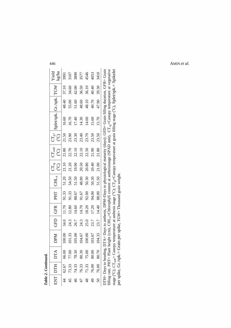
446 AMIN et al.
EN
T
DT
H
DT
A
DP
M
GF
D
GF
R
PH
T
CH
LA
C
Tvg
(oC
)
CT
anth
(oC
)
CT
g f
(oC
) S
ple
t/sp
k.
Gr.
/sp
k.
TG
W
Yie
ld
kg/h
a
44
62
.67
66
.00
10
0.0
0
34
.0
11
.70
91
.33
51
.20
21
.10
21
.80
21
.50
16
.60
48
.40
37
.10
39
91
45
73
.33
77
.00
10
1.3
3
24
.3
12
.80
91
.33
54
.50
21
.20
22
.70
23
.90
16
.70
55
.00
34
.60
31
07
46
74
.33
78
.30
10
5.0
0
26
.7
14
.60
88
.67
51
.50
19
.90
22
.10
23
.30
17
.40
51
.60
42
.00
38
90
47
76
.33
80
.30
10
4.6
7
24
.3
14
.70
91
.67
48
.80
20
.50
22
.10
23
.40
14
.30
48
.60
36
.50
35
77
48
71
.33
75
.00
10
0.0
0
25
.0
18
.20
92
.00
50
.30
20
.80
22
.50
23
.70
14
.60
48
.10
36
.10
45
46
49
76
.00
80
.00
10
3.6
7
23
.7
17
.20
94
.00
50
.30
20
.40
21
.90
23
.50
15
.60
40
.70
40
.40
40
53
50
76
.00
80
.70
10
4.3
3
23
.7
14
.40
88
.00
51
.50
21
.00
21
.80
23
.50
15
.70
47
.90
39
.30
34
10
DT
H=
Day
s to
hea
din
g,
DT
A=
Day
s to
anth
esi
s, D
PM
=D
ays
to p
hysi
olo
gic
al m
aturi
ty (
day
s);
GF
D=
Gra
in f
illi
ng d
ura
tio
n,
GF
R=
Gra
in
fill
ing r
ate,
PH
T=
Pla
nt
hei
gh
t (c
m),
CH
LA=
Chlo
rop
hyll
co
nte
nt
at a
nth
esis
stag
e (
SP
AD
unit
),
CT
vg=
Cano
py t
em
per
ature
at
veget
ativ
e
stag
e (o
C);
CT
anth
= C
ano
py t
em
per
ature
at
anth
esi
s st
age
(oC
); C
Tgf=
Cano
py t
em
per
ature
at
gra
in f
illi
ng s
tage
(oC
), S
ple
t/sp
k.=
Sp
ikel
et
per
sp
ike,
Gr.
/sp
k.=
Gra
in p
er s
pik
e, T
GW
= T
ho
usa
nd
gra
in w
eig
ht.
Ta
ble
2.
Co
nti
nu
ed.

VARIABILITY AND HERITABILITY ANALYSIS IN SPRING WHEAT 447
Thousand grain weight exhibited higher estimate of broad sense heritability
(55.3%) along with lower genetic advance in percent of mean (10.30) [Table 3].
Phenotypic selection may provide some improvement for this trait as there might
be presence of non-additive gene action. Chaturvedi and Gupta (1995) found
higher estimates of heritability for 1000-grain weight. Many other authors
reported high heritability along with high genetic advance for 1000-grain weight
(Sharma et al., 1995; Shoran, 1995; Vilhelmsen et al., 2001 and Ali et al., 2008).
Grain yield showed high estimate of broad sense heritability (69.10%) along with
moderate genetic advance in percent of mean (18.67) indicating the presence of
additive and non-additive gene action for the expression of this trait [Table 3].
There is a scope of phenotypic selection for the improvement of this trait. Many
authors found high heritability along with high to moderate genetic advance for
grain yield in wheat (Barma, 2005; Singh et al., 2006; Ali et al., 2008; Rahman,
2009).
Genotypic co-efficient of variation together with high heritability and genetic
advance are considered as good estimates of genetic gain to be expected in
making selection of superior genotypes on the basis of phenotypic performance.
Johnson et al., (1955) mentioned that high heritability along with high genetic
gain are more successful than the heritability alone to select desirable genotypes
with higher yield.Panse (1957) stated that high value of heritability with low
genetic advance indicated that the heritability was probably due to the effect of
non-additive gene action. The characters with high values of GCV, PCV, and
heritability accompanied by high genetic advance in percent of mean might be
transmitted to their progenies and therefore, phenotypic selection based on these
characters would be effective.
Estimated phenotypic coefficient of variation (PCV) and genotypic coefficient of
variation (GCV) revealed higher to moderate range of genetic variations for most
of the phenological and physiological traits. Grain filling period, grain filling
rate, grain yield, exhibited more than 10% GCV. DTH, DTA, CHLA, spikelets
spike-1
, grains spike-1
, TGW also had moderate range of PCV% and GCV%.
DPM, PHT, CTvg (oC), CTg (
oC), CTanth (
oC), had lower GCV estimate (<10%)
indicating narrow range of genetic variation. The PCV and corresponding GCV
estimates were close to each other for CHLA, DTA, DPM, DTH indicating less
influence of environment for the expression of these traits. On the other hand the
PCV estimate for GFD, GFR, PHT, CTvg (oC), CTanth (
oC), CTg (
oC), spikelets
spike-1
, grains spike-1
, TGW , and yield (kg/ha), were moderately higher to much
higher than corresponding GCV indicating that the environment had moderate to
major influence for the expression of these traits.
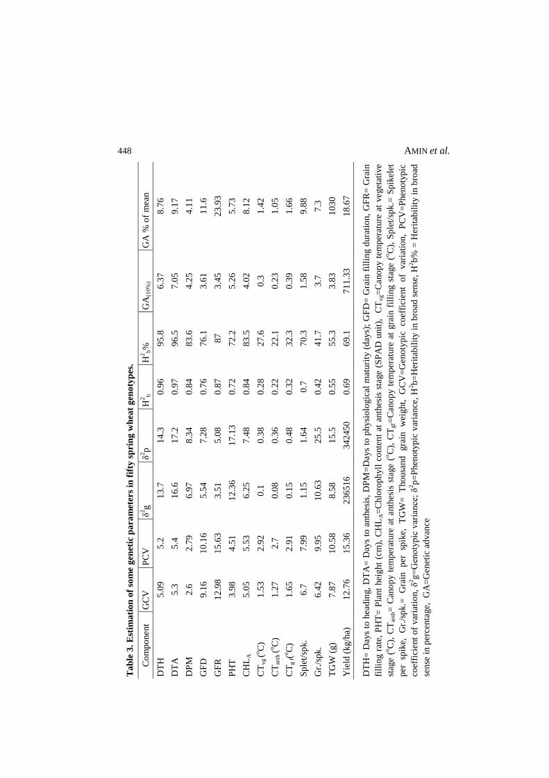
448 AMIN et al.
Ta
ble
3.
Est
ima
tio
n o
f so
me
gen
etic
pa
ram
eter
s in
fif
ty s
pri
ng
wh
eat
gen
oty
pes
.
Co
mp
onent
GC
V
PC
V
δ2g
δ
2p
H
2b
H2
b%
G
A(1
0%
) G
A %
of
mea
n
DT
H
5.0
9
5.2
1
3.7
1
4.3
0
.96
95
.8
6.3
7
8.7
6
DT
A
5.3
5
.4
16
.6
17
.2
0.9
7
96
.5
7.0
5
9.1
7
DP
M
2.6
2
.79
6.9
7
8.3
4
0.8
4
83
.6
4.2
5
4.1
1
GF
D
9.1
6
10
.16
5.5
4
7.2
8
0.7
6
76
.1
3.6
1
11
.6
GF
R
12
.98
15
.63
3.5
1
5.0
8
0.8
7
87
3.4
5
23
.93
PH
T
3.9
8
4.5
1
12
.36
17
.13
0.7
2
72
.2
5.2
6
5.7
3
CH
LA
5.0
5
5.5
3
6.2
5
7.4
8
0.8
4
83
.5
4.0
2
8.1
2
CT
vg (
oC
) 1
.53
2.9
2
0.1
0
.38
0.2
8
27
.6
0.3
1
.42
CT
anth
(oC
) 1
.27
2.7
0
.08
0.3
6
0.2
2
22
.1
0.2
3
1.0
5
CT
g f(o
C)
1.6
5
2.9
1
0.1
5
0.4
8
0.3
2
32
.3
0.3
9
1.6
6
Sp
let/
spk.
6.7
7
.99
1.1
5
1.6
4
0.7
7
0.3
1
.58
9.8
8
Gr.
/sp
k.
6.4
2
9.9
5
10
.63
25
.5
0.4
2
41
.7
3.7
7
.3
TG
W (
g)
7.8
7
10
.58
8.5
8
15
.5
0.5
5
55
.3
3.8
3
10
30
Yie
ld (
kg/h
a)
12
.76
15
.36
23
651
6
34
245
0
0.6
9
69
.1
71
1.3
3
18
.67
DT
H=
Day
s to
hea
din
g,
DT
A=
Day
s to
anth
esi
s, D
PM
=D
ays
to p
hysi
olo
gic
al m
aturi
ty (
day
s);
GF
D=
Gra
in f
illi
ng d
ura
tio
n,
GF
R=
Gra
in
fill
ing r
ate,
PH
T=
Pla
nt
hei
gh
t (c
m),
CH
LA=
Chlo
rop
hyll
co
nte
nt
at a
nth
esis
sta
ge
(SP
AD
unit
),
CT
vg=
Cano
py t
em
per
atu
re a
t veget
ativ
e
stag
e (o
C),
CT
anth
= C
ano
py t
emp
erat
ure
at
anth
esis
sta
ge
(oC
), C
Tgf=
Cano
py t
em
per
ature
at
gra
in f
illi
ng s
tage
(oC
), S
ple
t/sp
k.=
Sp
ikel
et
per
sp
ike,
G
r./s
pk.=
G
rain
p
er
spik
e,
TG
W=
T
ho
usa
nd
gra
in
wei
ght,
G
CV
=G
eno
typ
ic
coef
fici
ent
of
var
iati
on,
PC
V=
Phen
oty
pic
coef
fici
ent
of
var
iati
on,
δ2g=
Gen
oty
pic
var
iance
; δ
2p
=P
hen
oty
pic
var
iance
, H
2b
=H
erit
abil
ity i
n b
road
sen
se,
H2b
% =
Her
itab
ilit
y i
n b
road
sen
se i
n p
erce
nta
ge,
G
A=
Gen
etic
ad
van
ce

VARIABILITY AND HERITABILITY ANALYSIS IN SPRING WHEAT 449
High heritability along with higher genetic advance was observed for DTH,
DTA, DPM, GFD, GFR, PHT, CHLA, spikelets spike-1
, and yield (kg/ha)
indicated that direct phenotypic selection has good chances to bring some good
improvement in these traits. The remaining traits showed lower heritability
coupled with low genetic advance in percent of mean indicating that selection has
little to no chance for improvement. Considering variability among the
genotypes, heritability, genetic advance, percent co-efficient of variance, and
field performances, the genotypes G 3, G 10, G 11, G 12, G13, G 21, G 29, G 35,
G 38, G 40, and G 48 were found suitable for future breeding programme.
References
Allard, R. W. 1960. Principles of Plant Breeding. John Wiley and Sons. Inc. New York.
Ali, Y., B. Manzoor, J. Akhter, P. Monneveux and Z. Lateef. 2008. Genetic Variability,
Character Association and Diversity Studies in Wheat. Pak. J. Bot. 40(5): 2087-
2097.
Barma, N.C.D. 2005. Genetic study of morpho-physiological traits related to heat
tolerance in spring wheat. Ph.D. Thesis, Dept. of Genetics and Plant Breeding, BAU,
Mymensingh.
Barma, N. C. D., S. H. Khan, M. A. K. Mian and A. Islam. 1990. Variability and
Interrelationships of eight Quantitative Characters in Bread Wheat (Triticum
aestivum L.). Bangladesh J. Plant Breed. Genet. 3(1 & 2): 71-75.
Braun, H.J., T.S.Payne, A.I. Morgounov, M. van Ginkel, and S. Rajaram, (1998).The
challenge: one billion tons of wheat by 2020. In: AE. Slinkard (ed.), Proceedings
of the 9th International Wheat Genetics Symposium, Saskatoon, Canada, vol I, Pp.
33-40.
Burton, G. W. 1952. Quantitative inheritance in grasses. Proc. sixth Int. Grassland Cong.
1: 277-283.
Comstock, R.E. and H.F. Robinson. 1952. Genetic parameters, their estimation and
significance. Proc. sixth Int. Grassland Cong. 1: 284-291.
Chaturvedi, B. K. and R. R. Gupta. 1995. Selection parameters for some grain and quality
attributes in spring wheat (Triticum aestivum L.). Agric. Sci. Digest. 15(4): 186-190,
Karnal, India.
Falconar, D. S. 1989. Introduction to Quantitative Genetics. 2nd
Ed. English Language
Book Society/ Longman. P. 288.
Hanson, C. H., H. F. Robinson and R. E. Comstock. 1956. Biometrical studies of yield in
segregating population of Korean lespedeza. Agronomy Journal 48: 268-272.
Johnson, H. W., H. F. Robinson and R. E. Comstock. 1955. Estimation of genetic and
environmental variability in soybean. Agronomy Journal. 47: 314-318.
Panse, V. G. 1957. Genetics of quantitative characters in relation to plant breeding.
Indian J. Genet. 17:318-328.

450 AMIN et al.
Rahman, M.M. 2009. Genetic variability and genotypes-environment interaction in
wheat. M.S. Thesis, Bangabandhu Sheikh Mujibur Rahman Agricultural University,
Gazipur.
Reynolds, M. P., S. Nagaranjan, M. A. Razzaque and O. A. A. Ageeb (eds.). 1997. Using
canopy temperature depression to select for yield potential of wheat in heat- stressed
environments. Wheat Special Report No. 42. Mexico. D. F.: CIMMYT.
Reynolds, M. P., M. Balota, M. I. B. Delgado, I. Amani and R. A. Fischer. 1994.
Pyhsiological and morphological traits associated with spring wheat yield under hot,
irrigated conditions. Aust. J. Plant Physiol. 21: 717-730.
Sharma, D. J., R. K. Yadav and P. K. Sharma. 1995. Genetic variability and association
of some yield components in winter x spring nursery of wheat. Adv. in Pl. Sci.
8(l):95-99.
Shoran, J. 1995. Estimation of variability parameters and path coefficients for certain
metric traits in winter wheat (Triticum. aestivum L.). Indian J. Genet. 55(4): 399-
405.
Singh, K. N., K. Neeraj, V. Kumar and S. Tim. 2006. Genetic variability of wheat
(Triticum aestivum L.) lines for grain yield and component characters grown under
sodic and waterlogged conditions. Indian Journal of Agricultural Science. 76(7):
414-419.
Vasil, I.K. and O.D. Anderson, (1997). Genetic engineering of wheat gluten (review).
Trends in Plant Science, 2: 292-297.
Vilhelmsen, A.L., M.P. Reynolds, B. Skovmand, D. Mohan, K.N. Ruwali, S. Nagrajan
and O. Stoelen. 2001. Genetic diversity and heritability of heat tolerance traits in
wheat. Wheat Special Report. Mexico, D. F., CIMMYT.
ISSN 0258-7122
Bangladesh J. Agril. Res. 40(3): 451-463, September 2015
LARVICIDAL EFFICACY OF SOME INDIGENOUS PLANT EXTRACTS
AGAINST EPILACHNA BEETLE, EPILACHNA
VIGINTIOCTOPUNCTATA (FAB.) (COLEOPTERA: COCCINELLIDAE)
R. ARA1, M. A. A. BACHCHU
2, M. O. KULSUM
3 AND Z. I. SARKER
4
Abstract
The study was carried out to assess the larvicidal efficacies of some indigenous
plant seed extracts against epilachna beetle, Epilachna vigintioctopunctata in the
laboratory of the Department of Entomology, HSTU, Dinajpur, Bangladesh.
Petroleum ether and methanol solvent extracts of ata (Annona squamosa), neem
(Azadirachta indica), dhutura (Datura metel) and castor (Ricinus communis)
seeds were evaluated for their larvicidal properties against the larval stage of E.
vigintioctopunctata. The result revealed that all the tested plant extracts had
more or less insecticidal effect against the larvae and their progeny. Among the
plant extracts, ata seed extract in methanol solvent performed the highest
toxicity (LD50 value 0.031 mg/insect) in larval stage after 72 hours exposure
time. The effects of the extracts on fecundity, fertility and F1 adult emergence of
the epilachna beetle at doses 4.0, 2.0 and 1.0 ml/l of water including untreated
control were also evaluated. The result indicated that, among the extracts, ata
seed extract at maximum dose (4.0 ml/l water) showed the highest efficacy with
the inhibition of total eggs (74.1%), viable eggs (80.4%) and number of
emergent adult progeny (87.3%). The result also revealed that the number of
eggs, number of viable eggs and F1 progeny production decreased with the
increase of doses. All the treated doses effectively reduced the epilachna beetle
as compared to untreated control.
Keywords: Plant extracts, petroleum ether, methanol solvent, larval mortality,
Epilachna vigintioctopunctata.
Introduction
Two species of epilachna beetle viz. Epilachna vigintioctopunctata (Fab.) and
Epilachna dodecastigma (Wied.) are serious pests of vegetables in Bangladesh
(Khan et al., 2000). Epilachna beetles are locally known as hadda beetles and
common throughout the country and cause a considerable damage to a number of
solanaceous, cucurbitaceous and leguminous crops (Anam et al., 2006; Rahaman
et al., 2008; Islam, et al., 2011). Both adults and grubs feed voraciously by
scrapping the chlorophyll of the leaves, causing characteristics skeletonization of
the lamina. Affected leaves gradually dry and drop down (Srivastava and Butani,
1998).
1-3Department of Entomology, Hajee Mohammad Danesh Science and Technology
University (HSTU), Dinajpur, 4Breeding division, Wheat Research Centre, Nashipur,
Dinajpur, Bangladesh.

452 ARA et al.
Due to infestation of epilachna beetle about 80% of plants are damaged
depending on place and season for prevailing environmental conditions
(Rajagopal and Trivedi, 1989). The presence of this pest is one of the limiting
factors in the vegetable production causing qualitative as well as quantitative
losses. Synthetic chemical insecticides have been widely preferred to combat this
pest problem because of their quick knock-down effect. But due to some ill-
effects of the chemical insecticides, there have been numerous problems, such as
acute and chronic poisoning of applicators, farm workers, consumers, fishes,
birds and other wild life animals etc. (National Research Council, 2000; Rohani
et al., 2001). Substitutes are being strongly conceived whereby researchers are
now paying much emphasis on the biologically active indigenous plant products
as they are environmentally safe, biodegradable and cost effective. Plant extracts
contain botanical insecticides or phytochemicals that could be used to repel, deter
feeding, or limit reproduction and survival of various insect pest species
including coccinellid beetles (Rajagopal and Trivedi, 1989; Swaminathan et al.,
2010).
Using various plant extracts, attempts have been made to save such crops as
potato (Rajagopal and Trivedi, 1989), brinjal (Sreedevi et al., 1993; Ghatak and
Mondal, 2008), oilseed (Ahmed, 2007; Ahmed et al., 2010), cucumber (Mondal
and Ghatak, 2009) and bitter gourd (Rahaman et al., 2008) against the attacks of
the beetle. Ahmed (2007) reported that aqueous extract sprays of the castor oil
plant Ricinus communis L. (F. Euphorbiaceae) reduced Epilachna attack on
foliage. Subsequently, methanol extracts of R. communis were found to have
larvicidal properties against the mosquitoes Aedes aegypti (Zahir et al., 2009).
Anam et al., (2006) reported that neem oil significantly prolonged larval and
pupal periods and some of the treated larvae never reached to the pupae. Pupal
recovery and adult emergence were greatly reduced in treated larvae. The
aqueous extract of Calotropis procera showed strong repellent activity against
the Henosepilachna elaterii (Ahmed et al., 2006). The uses of plant products
against vegetable pests are scanty in Bangladesh. Therefore, an attempt was
made to find out the larvicidal efficacy of the seed extracts of neem, ata, dhutura
and castor against the larvae of epilachna beetle.
Materials and Method
Collection and preparation of test plant seed powder: The study was
conducted in the laboratory of the Department of Entomology, Hajee Mohammad
Danesh Science and Technology University (HSTU), Dinajpur, Bangladesh
during August 2012 to November 2012. Test plant materials, such as neem
(Azadirachta indica A. Juss.), ata (Annona squamosa L.), dhutura (Datura metel
L.) and castor (R. communis L.) seeds were collected from the villages of the
Dinajpur district. All seeds were collected at the ripening stage. Collected seeds

LARVICIDAL EFFICACY OF PLANT EXTRACTS AGAINST EPILACHNA BEETLE 453
were washed in the running tap water and then dried under shade in the
laboratory as breakdown of various compounds may occur in sunlight. The dried
seeds were then powdered in a hand grinding machine separately. Before
grinding the seeds were well-dried in an oven at 40ºC for six hours. A sieve of
60-mesh diameter was used to obtain the fine powder. Later each powder was
stored in plastic containers under laboratory condition for experimental use.
Preparation of seed extract: Hundred grams of different seed powders were
dissolved in 300 ml of pure methanol (polar) and petroleum ether (non-polar)
solvent separately and stirred for 30 minutes in a magnetic stirrer. The mixture
was then allowed to stand for 72 hours and shaking several intervals. Then, the
mixture was filtered through a filter paper (Whatman no. 42) and allowed to
evaporate the solvents in water bath at 700C. Finally, the oily crude extracts were
obtained. The oily extracts were preserved in tightly corked vials and stored in a
refrigerator for experimental use.
Rearing and mass culture of the test insect (E. vigintioctopunctata): In order
to obtain a huge number of beetles continuously for experimental use a mass
culture was maintained in cages with potted plant of bitter gourd. The adults of E.
vigintioctopunctata were collected from the infested bitter gourd plant cultivated
in the field of Entomology Department, HSTU campus. They were sexed and one
pair of beetle was released in each plant in the fine mesh nylon cages (45 cm x 35
cm x 60 cm) under laboratory conditions at 28±2°C and 81±2% RH for
oviposition. After oviposition adult beetles were transferred in different cages
and the egg masses were left undisturbed for hatching. After hatching the larvae
and pupae were reared up to adult emergence. For continuous supply of the
potted plants as food, bitter gourd seeds were sown in earthen pots every
alternate day. When the plants were fed by larvae in cages, the fresh plant pot
was placed attached to the adjacent pot, thus all the larvae moved to the fresh
one. The number of instars was determined by their shed skin. This procedure
was used to obtain a large number of larvae of the same instar (4th) at the same
time for experiments.
Experimental protocol
Effect of plant extract on the larval mortality (direct toxicity): Direct toxicity
tests on the larvae of epilachna beetle were conducted under laboratory
conditions at 28±2°C and 81±2% RH following Completely Randomized Design
(CRD). Different concentrations of crude extracts were prepared by diluting with
the respective solvents. The concentrations were 100, 50, 25, 12.5 and 6.25
mg/ml of each plant in each solvent. Before applying extracts, the larvae were
chilled for a period of 10 minutes in refrigerator. The immobilized larvae were
individually picked up and 10 micro-liter solutions of different concentrations

454 ARA et al.
(100, 50, 25, 12.5 and 6.25 mg/ml) were applied to the dorsal surface of the
thorax of each individual with the help of a micro syringe (Hamilton, USA). Ten
larvae were treated in one replication. Three replications were used in each dose.
The insects of control treatment were treated with the respective solvent only.
The insects were then transferred into 9.0 cm diameter Petri dishes containing
leaf disc of bitter gourd as food. Insect mortality was recorded at 24, 48 and 72
hours after treatment. The data were corrected by Abbott’s (1987) formula. The
probit analyses were done to estimate LD50 values with 95% fiducial limits.
Heterogeneity was tested by a chi-square test.
Effect of plant extracts on the fecundity, egg hatchability, and adult
population of F1 progeny (residual effect)
The seeds of neem, ata, dhutura and castor were extracted in two solvents
(petroleum spirit and methanol) for their residual effect on the fecundity, egg
hatchability, and adult population of F1 progeny. Each type of crude extract was
diluted with distilled water containing 0.01% nonidet to prepare different
concentrations of spray solution. The doses were 4.0, 2.0, and 1.0 ml/l of water
for each treatment. The total numbers of treatments were 25 and replication was
thrice for each dose. The test extracts were compared with untreated control.
The entire experiment was conducted with the potted bitter gourd plant. Bitter
gourd seeds were collected from regional BRAC seed centre, Dinajpur and
planted in earthen pot. To prevent the pest infestation, plants were covered with
mosquito net. Sprayings with different solutions were done at 40 days after
sowing (DAS) by a hand sprayer. After spraying each plant was marked with
marking card. To induce population build up one pair of 10-15 days old fresh
healthy adult beetles were released in each plant and kept for oviposition. The
total numbers of eggs in masses were counted and recorded after seven days with
the help of magnifying glass and then the parent beetles were removed.
Observations on total number of larvae, pupae and adult emergence (F1 progeny)
were also counted and recorded up to adult emergence.
Statistical analysis: The experiments were conducted using CRD. The data
obtained from the experiments were statistically analyzed by MSTAT-C
computer program. The means of the treatments were tested by DMRT. The
observed mortality data were corrected by Abbott’s (1987) formula and then
subjected to probit analysis.
Results and Discussion
Effect of plant seed extracts on larval mortality: The results of the larval
mortality for the estimation of LD50 values, 95% confidence limits, regression
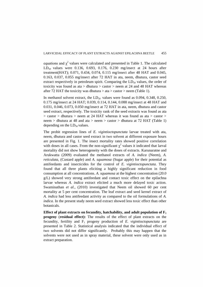
LARVICIDAL EFFICACY OF PLANT EXTRACTS AGAINST EPILACHNA BEETLE 455
equations and χ2 values were calculated and presented in Table 1. The calculated
LD50 values were 0.136, 0.693, 0.176, 0.230 mg/insect at 24 hours after
treatment(HAT); 0.071, 0.434, 0.074, 0.115 mg/insect after 48 HAT and 0.045,
0.163, 0.037, 0.055 mg/insect after 72 HAT in ata, neem, dhutura, castor seed
extract respectively in petroleum spirit. Comparing the LD50 values, the order of
toxicity was found as ata > dhutura > castor > neem at 24 and 48 HAT whereas
after 72 HAT the toxicity was dhutura > ata > castor > neem (Table 1).
In methanol solvent extract, the LD50 values were found as 0.094, 0.348, 0.250,
0.175 mg/insect at 24 HAT; 0.039, 0.114, 0.144, 0.088 mg/insect at 48 HAT and
0.031, 0.046, 0.073, 0.050 mg/insect at 72 HAT in ata, neem, dhutura and castor
seed extract, respectively. The toxicity rank of the seed extracts was found as ata
> castor > dhutura > neem at 24 HAT whereas it was found as ata > castor >
neem > dhutura at 48 and ata > neem > castor > dhutura at 72 HAT (Table 1)
depending on the LD50 values.
The probit regression lines of E. vigintioctopunctata larvae treated with ata,
neem, dhutura and castor seed extract in two solvent at different exposure hours
are presented in Fig. 1. The insect mortality rates showed positive correlation
with doses in all cases. From the non-significant χ2 values it indicated that larval
mortality did not show heterogeneity with the doses of extracts. Karunaratne and
Arukwatta (2009) evaluated the methanol extracts of A. indica (Neem), A.
reticulata, (Custard apple) and A. squamosa (Sugar apple) for their potential as
antifeedants and insecticides for the control of E. vigintioctopunctata. They
found that all three plants eliciting a highly significant reduction in food
consumption at all concentrations. A. squamosa at the highest concentration (20.0
g/L) showed very strong antifeedant and contact toxic effect on the epilachna
larvae whereas A. indica extract elicited a much more delayed toxic action.
Swaminathan et al., (2010) investigated that Neem oil showed 60 per cent
mortality at 5 per cent concentration. The leaf extract and seed kernel extract of
A. indica had less antifeedant activity as compared to the oil formulations of A.
indica. In the present study neem seed extract showed less toxic effect than other
botanicals.
Effect of plant extracts on fecundity, hatchability, and adult population of F1
progeny (residual effect): The results of the effect of plant extracts on the
fecundity, fertility and F1 progeny production of E. vigintioctopunctata are
presented in Table 2. Statistical analysis indicated that the individual effect of
two solvents did not differ significantly. Probably this may happen that the
solvents were not used as in spray material, these solvent were only used as in
extract preparation.

456 ARA et al.
Tab
le 1
. R
elati
ve
toxic
ity o
f d
iffe
ren
t in
dig
enou
s p
lan
t se
ed e
xtr
act
s of
two s
olv
ents
tre
ate
d a
gain
st E
pil
ach
na v
igin
tioct
opu
nct
ata
(F
ab
.)
So
lvent
use
d
Pla
nt
seed
D
ura
tio
n o
f
Tre
atm
ent
No
. o
f
larv
ae
use
d
LD
50
(mg/i
nse
ct)
95
% c
onfi
den
ce l
imit
Reg
ress
ion e
quat
ion
χ2
val
ue
(df
= 3
) L
ow
er
Up
per
Petroleum
spirit
Ata
24
HA
T
15
0
0.1
364
09
0
.06
02
26
0
.30
89
59
Y
= 4
.349
508
+ 0
.57
32
004
X
0.0
582
404
48
HA
T
15
0
0.0
705
88
0
.03
04
32
0
.16
37
28
Y
= 4
.455
248
+ 0
.64
18
457
X
0.1
351
719
72
HA
T
15
0
0.0
446
58
0
.01
70
03
0
.11
72
93
Y =
4.5
45
282
+ 0
.69
96
722
X
0.4
227
400
Cas
tor
24
HA
T
15
0
0.2
303
93
0
.08
51
89
0
.73
60
46
Y
= 4
.263
516
+ 0
.52
65
698
X
0.0
182
552
48
HA
T
15
0
0.1
154
83
0
.04
61
41
0
.28
90
32
Y
= 4
.458
756
+ 0
.50
93
98 X
0
.16
51
783
72
HA
T
15
0
0.0
553
76
0
.01
93
71
0
.15
83
00
Y =
4.5
72
763
+ 0
.57
47
69 X
0
.12
89
406
Dh
utu
ra
24
HA
T
15
0
0.1
760
29
0
.07
74
41
0
.40
01
26
Y
= 4
.252
675
+ 0
.59
99
796
X
0.0
089
731
48
HA
T
15
0
0.0
738
07
0
.03
53
77
0.1
539
82
Y
= 4
.374
619
+ 0
.72
04
061
X
0.2
571
945
72
HA
T
15
0
0.0
370
54
0
.01
22
58
0
.11
20
05
Y =
4.6
18
414
+ 0
.67
08
236
X
0.3
140
278
Nee
m
24
HA
T
15
0
0.6
932
45
0
.23
45
95
2
.04
85
86
Y
= 3
.340
462
+ 0
.90
14
887
X
0.3
007
021
48
HA
T
15
0
0.4
342
04
0
.14
84
63
1.2
699
02
Y
= 3
.849
556
+ 0
.70
24
786
X
0.1
576
462
72
HA
T
15
0
0.1
633
68
0
.08
03
71
0
.33
20
76
Y
= 4
.171
383
+ 0
.68
30
195
X
0.1
061
063
Methanol
Ata
24
HA
T
15
0
0.0
938
66
0
.04
28
69
0
.20
55
25
Y
= 4
.393
81
+ 0
.62
332
70
X
0.0
992
475
48
HA
T
15
0
0.0
386
96
0
.01
03
75
0
.14
43
21
Y
= 4
.676
89
+ 0
.54
981
85
X
0.0
756
526
72
HA
T
15
0
0.0
313
86
0
.01
08
29
0.0
909
59
Y
= 4
.621
701
+ 0
.76
15
78
X
0.2
303
925
Cas
tor
24
HA
T
15
0
0.1
748
67
0
.08
17
47
0
.37
40
60
Y
= 4
.193
177
+ 0
.64
92
46 X
0
.10
53
519
48
HA
T
15
0
0.0
881
85
0
.04
52
11
0
.17
20
06
Y
= 4
.294
052
+ 0
.74
67
22 X
0
.17
39
197
72
HA
T
15
0
0.0
503
67
0
.02
13
42
0
.11
88
68
Y
= 4
.481
58
+ 0
.73
833
39 X
0
.16
00
962
Dh
utu
ra
24
HA
T
15
0
0.2
504
07
0
.85
18
97
0.7
360
46
Y
= 4
.263
516
+ 0
.52
65
698
X
0.0
182
552
48
HA
T
15
0
0.1
441
36
0
.06
03
31
0
.34
43
51
Y
= 4
.374
189
+ 0
.54
00
64
X
0.2
390
728
72
HA
T
15
0
0.0
728
03
0
.02
94
30
0.1
800
97
Y
= 4
.492
859
+ 0
.58
82
30
X
0.3
903
656
Nee
m
24
HA
T
15
0
0.3
477
31
0
.10
71
07
1.1
289
34
Y
= 4
.121
894
+ 0
.56
97
39
X
0.1
259
551
48
HA
T
15
0
0.1
140
38
0
.05
41
75
0.2
400
51
Y
= 4
.331
665
+ 0
.63
22
64
X
0.0
293
164
72
HA
T
15
0
0.0
463
36
0
.01
63
86
0
.13
10
25
Y
= 4
.576
223
+ 0
.63
63
84 X
0
.26
07
088
HA
T =
Ho
ur
afte
r tr
eatm
ent,
Val
ues
wer
e b
ased
on f
ive
con
centr
atio
ns,
thre
e re
pli
cati
ons
of
10
lar
vae
eac
h.
χ2 =
Go
od
nes
s o
f fi
t, T
he
tab
ula
ted
val
ue
of
χ2 is
5.9
9 (
d.
f =
2 a
t 5
% l
evel
).

LARVICIDAL EFFICACY OF PLANT EXTRACTS AGAINST EPILACHNA BEETLE 457
Ta
ble
2.
Mea
n o
f eg
gs
laid
, v
iab
le e
gg
s, a
du
lt p
op
ula
tion
of
E.
vig
inti
oct
op
un
cta
ta r
eare
d i
n b
itte
r g
ou
rd p
lan
t tr
eate
d b
y d
iffe
ren
t
pla
nt
seed
extr
act
in
va
rio
us
do
ses.
So
lvent/
Pla
nt
seed
extr
act/
Do
ses
No
. o
f
egg
s
/inse
ct
inh
ibi-
tio
n r
ate
(%)
No
. o
f eg
g
hat
ched
inh
ibi-
tio
n r
ate
(%)
No
. o
f
larv
ae
inh
ibi-
tio
n r
ate
(%)
No
. o
f
pup
ae
inh
ibi-
tio
n r
ate
(%)
No
. o
f
adult
em
erged
inh
ibi-
tio
n r
ate
(%)
Pet
role
um
sp
irit
6
0.3
-
45
.7
- 2
9.3
-
17
.5
- 1
5.1
-
Met
hano
l 5
8.3
-
44
.1
- 2
8.6
-
16
.9
- 1
4.7
-
LS
D (
0.0
5)
NS
-
NS
-
NS
-
NS
-
NS
-
Ata
see
d e
xtr
act
(AS
E)
50
.9 c
4
5.4
3
8.6
c
51
.1
25
.5 c
5
8.0
1
5.4
c
59
.5
13
.6 c
5
8.8
Cas
tor
seed
extr
act
(CS
E)
52
.5 c
4
3.7
3
9.9
c
49
.5
26
.4 c
5
6.5
1
5.9
c
58
.2
14
.0 c
5
7.6
Dhutu
ra s
eed e
xtr
act
(DS
E)
67
.7 b
2
7.4
5
1.3
b
35
.1
32
.1 b
4
7.1
1
8.8
b
50
.5
16
.3 b
5
0.6
Nee
m s
eed
ex
trac
t (N
SE
) 6
6.2
b
29
.0
49
.7 b
3
7.1
3
1.7
b
47
.8
18
.8 b
5
0.5
1
5.7
b
52
.4
Co
ntr
ol
93
.3 a
0
7
9.0
a
0
60
.7 a
0
3
8.0
a
0
33
.0 a
0
LS
D (
0.0
5)
4.2
-
3.2
-
1.8
-
1.0
-
0.7
-
Do
se-1
(4
.0 m
l/li
tre)
3
2.3
d
65
.4
20
.6 d
7
3.9
1
0.8
d
82
.2
6.1
d
83
.9
5.3
d
83
.9
Do
se-2
(2
.0 m
l/li
tre)
4
5.4
c
51
.3
30
.8 c
6
1.0
1
6.7
c
72
.5
9.1
c
76
.1
7.9
c
76
.1
Do
se-3
(1
.0 m
l/li
tre)
6
6.3
b
28
.9
49
.1 b
3
7.8
2
7.7
b
54
.4
15
.7 b
5
8.7
1
3.5
b
59
.1
Co
ntr
ol
93
.3 a
0
7
9.0
a
0
60
.7 a
0
3
8.0
a
0
33
.0 a
0
LS
D (
0.0
5)
4.2
-
3.2
-
1.8
-
1.0
-
0.7
-
458 ARA et al.
So
lvent/
Pla
nt
seed
extr
act/
Do
ses
No
. o
f
egg
s
/inse
ct
inh
ibi-
tio
n r
ate
(%)
No
. o
f eg
g
hat
ched
inh
ibi-
tio
n r
ate
(%)
No
. o
f
larv
ae
inh
ibi-
tio
n r
ate
(%)
No
. o
f
pup
ae
inh
ibi-
tio
n r
ate
(%)
No
. o
f
adult
em
erged
inh
ibi-
tio
n r
ate
(%)
AS
E D
ose
-1 (
4.0
ml/
litr
e)
24
.2 h
7
4.1
1
5.5
g
80
.4
8.0
f
86
.8
4.7
g
87
.6
4.2
h
87
.3
AS
E D
ose
-2 (
2.0
ml/
litr
e)
34
.5 f
g
63
.0
23
.2 e
f 7
0.6
1
2.2
de
79
.9
7.0
e
81
.6
6.2
g
81
.2
AS
E D
ose
-3 (
1.0
ml/
litr
e)
51
.7 d
4
4.6
3
6.7
d
53
.5
21
.3 c
6
4.9
1
1.8
d
68
.9
10
.5 e
6
8.2
CS
E D
ose
-1 (
4.0
ml/
litr
e)
26
.5 g
h
71
.6
16
.8 f
g
78
.7
8.7
ef
8
5.7
5
.0 f
g
86
.8
4.5
h
86
.4
CS
E D
ose
-2 (
2.0
ml/
litr
e)
34
.2 f
g
63
.3
22
.8 e
f 7
1.1
1
2.5
d
79
.4
6.8
ef
82
.1
6.5
g
80
.3
CS
E
Do
se-3
(1
.0 m
l/li
tre)
5
6.2
d
39
.8
40
.8 d
4
8.4
2
3.8
c
60
.8
13
.8 c
6
3.7
1
2.2
d
63
.0
DS
E D
ose
-1 (
4.0
ml/
litr
e)
35
.7 e
f 6
1.7
2
3.3
e
70
.5
12
.0 d
e 8
0.2
6
.8 e
f 8
2.1
6
.0 g
8
1.8
DS
E D
ose
-2 (
2.0
ml/
litr
e)
57
.5 d
3
8.4
3
9.7
d
49
.7
21
.3 c
6
4.9
1
1.5
d
69
.7
9.8
ef
70
.3
DS
E D
ose
-3 (
1.0
ml/
litr
e)
84
.2 b
9
.8
63
.3 b
1
9.9
3
4.5
b
43
.2
19
.0 b
5
0.0
1
6.3
b
50
.6
NS
E D
ose
-1 (
4.0
ml/
litr
e)
43
.0 e
5
3.9
2
6.8
e
66
.1
14
.5 d
7
6.1
7
.8 e
7
9.5
6
.3 g
8
0.9
NS
E D
ose
-2 (
2.0
ml/
litr
e)
55
.3 d
4
0.7
3
7.5
d
52
.5
20
.7 c
6
5.9
1
1.2
d
70
.5
9.0
f
72
.7
NS
E D
ose
-3 (
1.0
ml/
litr
e)
73
.0 c
2
1.8
5
5.5
c
29
.7
31
.0 b
4
8.9
1
8.0
b
52
.6
14
.8 c
5
5.2
Co
ntr
ol
93
.3 a
0
7
9.0
a
0
60
.7 a
0
3
8.0
a
0
33
.0 a
0
* W
ithin
co
lum
n v
alues
foll
ow
ed b
y s
am
e le
tter
(s)
are
no
t si
gn
ific
antl
y d
iffe
rent
by D
MR
T a
t 5
% l
evel
of
pro
bab
ilit
y.
AS
E-
Ata
see
d e
xtr
act,
CS
E-
Cas
tor
seed
extr
act,
DS
E-
Dh
utu
ra s
eed
extr
act
and
NS
E-N
eem
see
d e
xtr
act.
Ta
ble
2.
Co
nti
nu
ed.
LARVICIDAL EFFICACY OF PLANT EXTRACTS AGAINST EPILACHNA BEETLE 459
The individual effects of plant extracts on the fecundity, fertility and F1 progeny
production of E. vigintioctopunctata were significantly different among the plant
extracts. Among the extracts, ata seed extracts showed maximum efficacy to
produce the lowest number of eggs (50.9), viable eggs (38.6) and population
production (13.6) followed by castor seed extract. On the other hand, dhutura
seed extracts showed the highest number of eggs (67.7), viable eggs (51.3) and
population production (16.3). The inhibition rate of the plant extracts ranged
from 27.4 to 45.4 % for the number of eggs per insect and 35.1 to 51.1% for the
number of egg hatched. The per cent larval and pupal inhibition was found 47.1
to 58.0 and 50.5 to 59.5 in all tested plant extract while no larval and pupal
inhibition was found in control treatment. Similarly, adult emergence inhibition
was found 50.6 to 58.8 % among the all the tested plant extracts whereas no per
cent inhibition of adult emergence was observed in control treatment. On the
basis of fecundity, hatchability, and adult population of F1 progeny the order of
toxicity was found as ata > castor > neem > dhutura.
The lowest average numbers of eggs laid, eggs hatched and population
production were observed in the highest dose of all plant extracts (4.0 ml/l) and
the highest numbers of eggs laid, eggs hatched and population production were
found in control (Table 2). The present result indicates that the fecundity, fertility
and population production decreased with the increased doses. Statistical analysis
showed that all the doses of the plant extracts differed significantly over control
and also among the plant extracts (Table 2). The per cent of the highest egg
laying inhibition rate was observed in highest dose (4.0 ml/l) and lowest was in
lowest dose (1.0 ml/l), whereas no egg laying inhibition rate was observed in the
control treatment. Similar results were found in per cent inhibition of egg hatch,
larval population, pupal population and adult emergence. (Table 2).
The ata seed extract showed the highest efficacy in producing the lowest number
of eggs per insect, viable eggs and F1 progeny productions in the highest dose
(4.0 ml/l). Similarly, ata showed the highest inhibition (%) rate in egg hatch,
larval population, pupal population and adult emergence (Table 2).
Reddy et al., (1990) reported that petroleum spirit (1%) extracts of A. indica and
A. squamosa reduced the number of H. vigintioctopunctata larvae infesting
brinjal by 88.0 and 92.99%; 85.98 and 91.02% at 24 and 72 hours after spraying,
respectively. Similarly, Rao et al., (1990) observed that extracts of A. squamosa,
Argemone mexicana, Calotropis gigantea, D. stramonium, Eucalyptus globulus,
Pongamia glabra and R. communis (0.5%) produced cent per cent protection
against second instar larvae of H. vigintioctopunctata. Mondal and Ghatak (2009)
found that seed extract of A. squamosa in methanol solvent achieved the highest
extent of 76.37% population reduction at 3ml/l of water followed by 64% in
Neem Azal at 5ml/l of water and 57% in petroleum spirit extracts of rhizome of
Acorus calamus at 2ml/l of water against H. vigintioctopunctata. The overall

460 ARA et al.
result of the present study achieved the bioefficacy of all the tested plant seed
extracts against E. vigintioctopunctata but among these, ata seed extract showed
the highest effect in reducing fecundity, hatchability and adult emergence of the
pest.
Fig. 1. Relation between log doses and probit mortality for different plant extracts against
larvae of E. vigintioctopunctata [A= Petroleun spirit of ata, B= methanol extract of ata,
C= Petroleun spirit of neem, D= methanol extract of neem, E= Petroleun spirit of
dhutura, F= methanol extract of dhutura, G= Petroleun spirit of castor H= methanol
extract of castor].
LARVICIDAL EFFICACY OF PLANT EXTRACTS AGAINST EPILACHNA BEETLE 461
Babu et al., (1998) reported that the seeds of A. squamosa were found to have
insecticidal properties. The larval mortality is probably due to the presence of
bioactive chemical components in plant products. The biological activity of ata
seed extracts might be attributed to its several alkaloids contents, such as
Anonaine, Squamocins B to N, Annotemoyin-1, Annotemoyin-2, Squamocin,
Cholesterol and Glucopyranoside etc. (Pandey and Brave, 2011) which might
cause mortality to insects.
Conclusion
The present result indicates the larvicidal efficacy of methanol and petroleum
spirit seed extracts of ata, neem, dhutura and castor against E. vigintioctopunctata
with some promising information on the direct toxicity on the larval mortality
and residual toxicity against the fecundity, fertility and F1 progeny production.
The mortality increased with increasing doses and exposure time. The dhutura
seed extract in petroleum spirit showed the highest toxicity in larval stages
whereas in methanol solvent, ata and castor seed extract achieved the highest
toxicity at 72 hours exposure time. The results revealed that among the extracts,
ata seed extract at maximum dose (4.0 ml/l water) showed the highest efficacy
with the inhibition of total eggs laid, viable eggs and the number of emergence of
F1 adult progeny. All the treated doses effectively reduced the epilachna beetle as
compared to untreated control.
Acknowledgment
This investigation is supported by financial grant received from the University
Grants Commission (UGC), Bangladesh which is gratefully acknowledged.
References
Abbott, W. S. 1987. A method of computing the effectiveness of an insecticide.
J. American Mosquito control Assoc. 3: 302-303.
Ahmed, K. N. 2007. Effect of biopesticides in the suppression of major insect pests and
yield of oilseed crops under different climatic conditions in Bangladesh. Proc. Natl.
Symp. Plant Protection-Technology Interface, Assoc. Adv. Plant Protection, Bidhan
Chandra Agricultural University, West Bengal, India, December 28-29, Pp. 81-82.
Ahmed, K. N., S. H. A. Pramanik, M. Khatun, A. Nargis and M. R. Hasan. 2010.
Efficacy of plant extracts in the suppression of insect pests and their effect on the
yield of sunflower crop under different climatic conditions. J. Plant Prot. Sci. 2(1):
53-58.
Ahmed, U. A. M., S. Zuhua, N. H. H. Bashier, K. Muafi, H. Zhongping and G. Yuling.
2006. Evaluation of insecticidal potentialities of aqueous extracts from Calotropis
procera Ait. against Henosepilachna elaterii Rossi. J. Applied Sci. 6: 2466-2470.
462 ARA et al.
Anam, M., M. Ahmad and M. A. Haque. 2006. Efficacy of neem oil on the biology and
food consumption of epilachna beetle, Epilachna dodecastigma (Weid.).
J. Agric. Rural Dev. 4(1&2): 83-88.
Babu, P. B. S., J. M. Rao and B. Joy. 1998. Effect of crude oils of Annona squamosa and
A. reticulata on feeding and development of Spodoptera litura (Fab.) larvae.
J. Insect Sci. 11: 184-185.
Ghatak, S.S. and S. Mondal. 2008. Feasibility of using plant products and biopesticides
against epilachna beetle, Henosepilachna vigintioctopunctata (Fab.), infecting
brinjal. Indian J. Entomol. 70(3): 278-279.
Islam, K., M. S. Islam and Z. Ferdousi. 2011. Control of Epilachna vigintioctopuntata
Fab. (Coleoptera: Coccinellidae) using some indigenous plant extracts.
J. Life Earth Sci. 6: 75-80.
Karunaratne, M. M. S. C. and A. P. K. M. C. P. Arukwatta. 2009. Efficacy of three plant
species on the mortality and food consumption of Epilachna vigintioctopunctata.
Vidyodaya J. Sci. 14: 167-176.
Khan, M. H., B. N. Islam, A. K. M. M. Rahman and M. L. Rahman. 2000. Life table and
the rate of food consumption of epilachna beetle, Epilachna dodecastigma (Wied.)
on different host plant species in laboratory condition. Bangladesh J. Ent. 10(1-2):
63-70.
Mondal, S. and S. S. Ghatak. 2009. Bioefficacy of some indigenous plant extracts against
epilachna beetle (Henosepilachna vigintioctopunctata Fabr.) infesting cucumber.
J. Plant Protect. Sci. 1(1):71-75.
National Research Council. 2000. The future role of pesticides in US Agriculture.
National Academic Press. Washington, DC. P. 323.
Pandey, N. and D. Brave. 2011. Phytochemical and pharmacological review on Annona
squamosa Linn. Int. J. Res. Phar. Bio. Sci. 2(4): 1404 – 1412.
Rahaman, M. A., M. D. H. Prodhan and A. K. M. Maula. 2008. Effect of botanical and
synthetic pesticides in controlling Epilachna beetle and the yield of bitter gourd.
Int. J. Sustain. Crop Prod. 3(5): 23-26.
Rajagopal, D. and T. P. Trivedi. 1989. Status, bioecology and management of epilachna
beetle, Epilachna vigintioctopunctata (Fab.) (Coleoptera: Coccinellidae) on potato in
India. Int. J.Pest Manage. 35(4): 410 - 413.
Rao, S. M., K. C. Chitra, D. Gunesekhar and P. K. Rao. 1990. Antifeedent properties of
certain plant extracts against second stage larva of Henosepilachna
vigintioctopunctata Fabricus. Indian J. Entomol. 52(4): 681-685.
Reddy, P. V. R., K. C. Chitra and P. K. Rao. 1990. Field evaluation of certain plant
extracts for the control of brinjal spotted leaf beetle, Henosepilachna
vigintioctopunctata. J. Insect Sci. 3: 194-195.
Rohani, A., W. L. Chu, L. Saadiyah, H. L. Lee and S. M. Phang. 2001. Insecticide
resistance status of Aedes albopietus and Aedes aegypti collected from urban and
rural in major towns of Malaysia. Trop. Biomed. 18(1): 29-39.
LARVICIDAL EFFICACY OF PLANT EXTRACTS AGAINST EPILACHNA BEETLE 463
Sreedevi, K., K. C. Chitra and K. Rao. 1993. Effect of certain plant extracts against
brinjal leaf beetle, Henosepilachna vigintioctopunctata Fab. under greenhouse
conditions. Indian J. Entomol. 55(3): 329-331.
Srivastava, K. P. and D. Butani. 1998. Pest management in vegetable. Research
Periodical and Book Publishing House, Pp. 197-225.
Swaminathan, R., M. Sumon and T. Hussain. 2010. Antifeedent activity of some
biopesticides on Henosepilachna vigintioctopunctata (Fab.) (Coleoptera:
Coccinellidae). J. Biopest. 3 (1 special issue): 77-88.
Zahir, A. A., A. A. Rahuman, C. Kamara, A. Bagavan, G. Elango, A. Sanganan and B.
Kumar. 2009. Laboratory determination of efficacy of indigenous plant extracts for
parasites control. Parasitol. Res. 105: 453-461.

464 ARA et al.

ISSN 0258-7122
Bangladesh J. Agril. Res. 40(3): 465-478, September 2015
EFFECT OF PLANTING DATES ON THE YIELD OF
BROCCOLI GENOTYPES
M. A. HAFIZ1, A. BISWAS
2, M. ZAKARIA
3, J. HASSAN
4 AND N. A. IVY
5
Abstract
This experiment was conducted during September, 2011 to March, 2012 in the
experimental field of Department of Horticulture, Bangabandhu Sheikh Mujibur
Rahman Agricultural University (BSMRAU), Gazipur to find out the effect of
planting date on the yield of broccoli genotypes. There were five genotypes viz.
Early green, Forest green, Green calabrese, Premium crop and Green king and
four planting dates viz. 2 October, 27 October, 21 November and 16 December.
The treatment effects were statistically analyzed and found significant in most of
the characters studied. Genotype Green calabrese was the highest in average
plant height (53.70 cm). Green king produced the maximum spread diameter
(69.23 cm), stem diameter (30.35 mm) and early initiation of floral head.
Genotype Early green performed the best regarding head weight (343.87 g),
yield per plant (477.4 g) and yield (19.10 t/ha). Broccoli planted on 21
November initiated early flower head, maximum head diameter (16.99 cm),
head weight (314.49 g), yield per plant (453.64 g) and total yield (18.15 t/ha).
The genotype Early green planted on 21 November showed the best
performance in yield per plant (580.17 g) and yield hectare (23.21 t/ha).
Keywords: Broccoli genotype(s), planting date, yield.
Introduction
Broccoli (Brassica oleracea var. italica L.), is an important member of “Cole”
crops, belongs to the family Brassicaceae. Broccoli originated from west Europe
(Prasad and Kumer, 1999). The word “Cole” means a group of highly
differentiated plants originated from a single wild Brassica oleracea var.
oleracea (Sylvestris L.) commonly known as wild cabbage (Bose and Som,
1986). Cole crops are the most widely grown vegetables in the temperate zones.
After the Second World War these have spread rapidly to both tropical and sub-
tropical areas and cabbage has increased in Africa by 31.5% and in Asia by 8.9%
compared to the total increase in the world by 5.8% from 1970 to 1980. In
Bangladesh, broccoli was introduced about two decades ago.
1MS Student, Department of Horticulture, Bangabandhu Sheikh Mujibur Rahman
Agricultural University, Gazipur, Bangladesh; 2
Scientific officer, Regional Agricultural
Research Station, Bangladesh Agricultural Research Institute (BARI), Jessore,
Bangladesh; 3Associate professor and
4Assitant professor, Department of Horticulture,
Bangabandhu Sheikh Mujibur Rahman Agricultural University, Gazipur, Bangladesh; 5Associate professor, Department of Genetics and Plant Breeding, Bangabandhu Sheikh
Mujibur Rahman Agricultural University, Gazipur, Bangladesh.
466 HAFIZ et al.
Broccoli is grown in winter season in Bangladesh as an annual crop. It is
environmentally better adapted and can withstand comparatively high
temperature than cauliflower (Rashid et al., 1976). Its wider environmental
adaptability, higher nutritive value, good taste and less risk to crop failure due to
various biotic and abiotic factors indicate that there is enough scope for its
promotional efforts. Its popularity to the consumers of urban area is increasing
day by day in our country. But its cultivation has not spread much beyond the
farms of different agricultural organizations. This is mainly due to the lack of
awareness among the people about its importance and lack of available
information production technology about it. Cultivation of broccoli in our
country are confined into a very limited area with a minimum production and its
average yield is only about 10.5 metric tons per hectare (Anon., 2004) which is
very low compared to other broccoli growing countries like 24 t/ha in Italy, 20
t/ha in Japan and 18 t/ha in Turkey (Ahmed et al., 2004).
The planting dates have significant effect on yield and other yield contributing
characters of broccoli. The yield decreased with delay planting. Head yield is
higher when crops are planted earlier and show a linear decreasing trend with
delay in planting dates (Bianco et al., 1996). Early planted crops resulted in
longer duration and produced taller plants with more number of leaves, higher
plant spread and more leaf size index as well as the lowest percentage of
abnormal curds than late planted crops and finally attributed to higher curd yield
(Gautam et al., 1998). So there is enough scope to identify the optimum planting
date to maximize the broccoli yield.
Broccoli genotypes have also significant effect on yield of broccoli. Cultivar
“Captain” produced the highest total yield as well as top and lateral head yields,
the largest top head weight and marked earliness which was followed by cultivars
Lucky, General, Griffen, Liberty and Milady (Toth et al., 2007). Several broccoli
genotypes are cultivated in our country those differ in yield. So it is essential to
identify high yielding genotypes to maximize broccoli yield. Therefore, the
present experiment was undertaken to find out optimum planting date and
appropriate genotype for maximum yield of Broccoli.
Materials and Method
The experiment was conducted at the Horticultural Research Farm, BSMRAU,
Gazipur during September, 2011 to March, 2012. The location of the
experimental site was at the centre of Madhupur Tract (24.090N latitude and
90.260E longitudes) at 8.5m above the sea level (Anon., 1995). The soil of the
experimental field was silty clay of shallow Red Brown Terrace type under Salna

EFFECT OF PLANTING DATES ON THE YIELD OF BROCCOLI GENOTYPES 467
Series of Madhupur Tract in agroecological zone (AEZ) 28 (Brammer,1971 and
Saheed,1984). The soil contained pH of 6.4 (Anon., 1998 and Haider et al.,
1991). There were four planting dates viz. 2 October, 27 October, 21 November
and 16 December and five genotypes viz. Early green, Forest green, Green
calabrase, Premium crop and Green king. The field experiment was laid out in a
factorial Randomized Complete Block Design with three replications. The unit
plot size was 4m x 1.5m. The genotypes of broccoli were collected from the
market of Siddique bazaar of Dhaka. The land was manured and fertilized with
N, P, K and Molybdenum as Cowdung, Urea, TSP, MoP and Molybdenum @
1500, 210, 120, 100 and 1kg/ha, respectively. The entire amount of Cow dung,
TSP, MoP and Molybdenum were applied at the time of final land preparation
and the entire urea was applied as top dressing in two equal split at 15 and 30
days after transplanting. Healthy and uniform 30 days old seedlings were
transplanted in the main field at each date of planting maintaining a spacing of
50 cm x 50 cm. Weeding, irrigation and other cultural practices were done as and
when necessary. Data were recorded from randomly selected plants for
individual plant performance and from total plot for per hectare yield. Collected
data were statistically analyzed by MSTATC.
Results and Discussion
Plant height
Significant variation in plant height was observed due to different planting dates
(Table 1). The highest plant height was obtained from 2 October planting at 15,
25 and 35 DAT (30.10, 40.75 and 54.83 cm, respectively) while it was the
minimum with delayed planting i.e. 16 December). This result was in agreement
with the result obtained by Ahmed and Abdullah (1986) who found taller plant of
broccoli from earlier planting than late planting.
Plant height varied significantly at 15, 25 and 35 DAT among the genotypes
(Table 1). The highest plant height (31.42 and 39.20cm) was recorded from the
genotype Premium at 15 and 25 DAT, respectively. At 35 DAT, Green calabrese
produced the tallest plant (53.70cm), which was statistically identical to Premium
(51.66 cm). At 15 DAT, the lowest plant height (26.81 cm) was obtained from
Green calabrese, which was statistically similar to Green king (27.70 cm) and
Forest green (27.11 cm). But at 25 and 35 DAT, Forest green produced the
lowest plant height as 34.05 and 46.07 cm, respectively. Variation in plant height
may be due to the difference in genetic make-up of broccoli genotypes.
The interaction effect between genotypes and planting dates varied significantly
at 15 DAT, but it did not vary significantly at 25 and 35 DAT (Table 2). The
highest plant height (34.50 cm) was recorded from the genotype Premium
planted on 27 October which was similar to G4P3 (32.50 cm) and the lowest

468 HAFIZ et al.
Ta
ble
1.
Eff
ect
of
gen
oty
pes
an
d p
lan
tin
g d
ate
s o
n p
lan
t h
eig
ht,
sp
rea
d d
iam
eter
an
d d
iam
eter
of
stem
of
bro
cco
li p
lan
t a
t
dif
feren
t D
AT
s.
Tre
atm
ents
P
lant
hei
ght
(cm
) S
pre
ad d
iam
eter
(cm
) D
iam
eter
of
stem
(m
m)
15
DA
T
25
DA
T
35
DA
T
15
DA
T
25
DA
T
35
DA
T
15
DA
T
25
DA
T
35
DA
T
Gen
oty
pes
Ear
ly g
reen
(G
1)
29
.31 b
3
7.3
0 b
4
8.2
7 b
3
2.8
9 c
d
52
.14 c
d
63
.89 b
1
0.4
3 b
1
7.6
3 c
2
7.5
4 c
Fo
rest
gre
en (
G2)
27
.11 c
3
4.0
5 c
4
6.0
7 b
3
6.0
5 a
5
5.5
8 a
6
8.5
5 a
1
1.2
8 a
1
8.8
0 b
2
8.2
3 b
c
Gre
en c
alab
rese
(G
3)
26
.81 c
3
6.8
0 b
5
3.7
0 a
3
1.9
8 d
5
1.7
3 d
6
8.3
2 a
8
.40
c
13
.93 d
2
2.3
6 d
Pre
miu
m (
G4)
31
.42 a
3
9.2
0 a
5
1.6
6 a
3
3.8
8 b
c 5
3.4
1 b
c 6
4.6
5 b
1
0.5
4 b
1
9.2
1 b
2
8.9
8 b
Gre
en k
ing (
G5)
27
.70 c
3
7.0
7 b
4
6.4
4 b
3
5.1
2 a
b
54
.56 a
b
69
.23 a
1
1.7
3 a
2
1.0
6 a
3
0.3
5 a
Pla
nti
ng
tim
e
2 O
cto
ber
(P
1)
30
.10 a
4
0.7
5 a
5
4.8
3 a
4
1.4
0 a
6
0.9
9 a
7
7.0
3 a
1
0.5
4 b
1
9.0
1 a
2
8.3
4 a
27
Oct
ob
er (
P2)
29
.41 a
3
8.9
6 b
4
9.0
2 b
3
8.7
2 b
5
1.8
1 b
6
9.0
9 b
1
1.1
7 a
1
9.8
5 a
2
7.9
9 a
b
21
N
ovem
ber
(P
3)
27
.23 b
3
6.7
9 c
4
6.6
0 c
3
7.5
9 b
5
0.2
3 c
6
1.4
6 c
1
0.7
9 a
b
17
.33 b
2
6.4
7 c
16
Dec
emb
er (
P4)
27
.13 b
3
1.0
3 d
4
6.4
6 c
1
8.2
3 c
5
0.9
1 b
c 6
0.1
2 d
9
.40
c
16
.32 c
2
7.1
6 b
c
CV
(%
) 6
.13
5.8
9
5.1
8
6.1
5
3.3
7
2.6
0
5.7
1
6.6
2
5.4
2
Mea
ns
bea
rin
g s
am
e le
tter
(s)
in a
co
lum
n d
o n
ot
dif
fer
sign
ific
antl
y a
t 1
% l
evel
of
pro
bab
ilit
y.
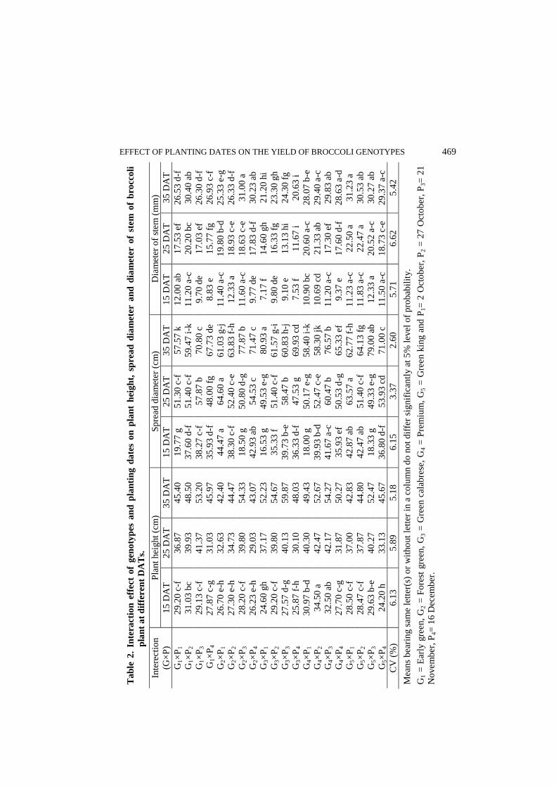
EFFECT OF PLANTING DATES ON THE YIELD OF BROCCOLI GENOTYPES 469
Ta
ble
2.
Inte
ract
ion
eff
ect
of
gen
oty
pes
an
d p
lan
tin
g d
ate
s o
n p
lan
t h
eig
ht,
sp
rea
d d
iam
eter
an
d d
iam
eter
of
stem
of
bro
cco
li
pla
nt
at
dif
feren
t D
AT
s.
Inte
rect
ion
(G×
P)
Pla
nt
hei
ght
(cm
) S
pre
ad d
iam
eter
(cm
) D
iam
eter
of
stem
(m
m)
15
DA
T
25
DA
T
35
DA
T
15
DA
T
25
DA
T
35
DA
T
15
DA
T
25
DA
T
35
DA
T
G1×
P1
29
.20 c
-f
36
.87
45
.40
19
.77 g
5
1.3
0 c
-f
57
.57 k
1
2.0
0 a
b
17
.53 e
f 2
6.5
3 d
-f
G1×
P2
31
.03 b
c 3
9.9
3
48
.50
37
.60 d
-f
51
.40 c
-f
59
.47 i
-k
11
.20 a
-c
20
.20 b
c 3
0.4
0 a
b
G1×
P3
29
.13 c
-f
41
.37
53
.20
38
.27 c
-f
57
.87 b
7
0.8
0 c
9
.70
de
17
.03 e
f 2
6.3
0 d
-f
G1×
P4
27
.87 c
-g
31
.03
45
.97
35
.93 d
-f
48
.00 f
g
67
.73 d
e 8
.83
e
15
.77 f
g
26
.93 c
-f
G2×
P1
26
.70 e
-h
32
.63
42
.40
44
.47 a
6
4.6
0 a
6
1.0
3 g
-j
11
.40 a
-c
19
.80 b
-d
25
.33 e
-g
G2×
P2
27
.30 e
-h
34
.73
44
.47
38
.30 c
-f
52
.40 c
-e
63
.83 f
-h
12
.33 a
1
8.9
3 c
-e
26
.33 d
-f
G2×
P3
28
.20 c
-f
39
.80
54
.33
18
.50 g
5
0.8
0 d
-g
77
.87 b
1
1.6
0 a
-c
18
.63 c
-e
31
.00 a
G2×
P4
26
.23 e
-h
29
.03
43
.07
42
.93 a
b
54
.53 c
7
1.4
7 c
9
.77
de
17
.83 d
-f
30
.23 a
b
G3×
P1
24
.60 g
h
37
.17
52
.23
16
.53 g
4
9.5
3 e
-g
80
.93 a
7
.17
f
14
.60 g
h
21
.20 h
i
G3×
P2
29
.20 c
-f
39
.80
54
.67
35
.33 f
5
1.4
0 c
-f
61
.57 g
-i
9.8
0 d
e 1
6.3
3 f
g
23
.30 g
h
G3×
P3
27
.57 d
-g
40
.13
59
.87
39
.73 b
-e
58
.47 b
6
0.8
3 h
-j
9.1
0 e
1
3.1
3 h
i 2
4.3
0 f
g
G3×
P4
25
.87 f
-h
30
.10
48
.03
36
.33 d
-f
47
.53 g
6
9.9
3 c
d
7.5
3 f
1
1.6
7 i
2
0.6
3 i
G4×
P1
30
.97 b
-d
40
.30
49
.43
18
.00 g
5
0.1
7 e
-g
58
.40 i
-k
10
.90 b
c 2
0.6
0 a
-c
28
.07 b
-e
G4×
P2
34
.50 a
4
2.4
7
52
.67
39
.93 b
-d
52
.47 c
-e
58
.30 j
k
10
.69 c
d
21
.33 a
b
29
.40 a
-c
G4×
P3
32
.50 a
b
42
.17
54
.27
41
.67 a
-c
60
.47 b
7
6.5
7 b
1
1.2
0 a
-c
17
.30 e
f 2
9.8
3 a
b
G4×
P4
27
.70 c
-g
31
.87
50
.27
35
.93 e
f 5
0.5
3 d
-g
65
.33 e
f 9
.37
e
17
.60 d
-f
28
.63 a
-d
G5×
P1
28
.50 c
-f
37
.00
42
.83
42
.87 a
b
63
.57 a
6
2.7
7 f
-h
11
.23 a
-c
22
.50 a
3
1.2
3 a
G5×
P2
28
.47 c
-f
37
.87
44
.80
42
.47 a
b
51
.40 c
-f
64
.13 f
g
11
.83 a
-c
22
.47 a
3
0.5
3 a
b
G5×
P3
29
.63 b
-e
40
.27
52
.47
18
.33 g
4
9.3
3 e
-g
79
.00 a
b
12
.33 a
2
0.5
2 a
-c
30
.27 a
b
G5×
P4
24
.20 h
3
3.1
3
45
.67
36
.80 d
-f
53
.93 c
d
71
.00 c
1
1.5
0 a
-c
18
.73 c
-e
29
.37 a
-c
CV
(%
) 6
.13
5.8
9
5.1
8
6.1
5
3.3
7
2.6
0
5.7
1
6.6
2
5.4
2
Mea
ns
bea
rin
g s
am
e le
tter
(s)
or
wit
ho
ut
lett
er i
n a
co
lum
n d
o n
ot
dif
fer
sig
nif
ican
tly a
t 5
% l
evel
of
pro
bab
ilit
y.
G1 =
Ear
ly g
reen
, G
2 =
Fo
rest
gre
en,
G3 =
Gre
en c
alab
rese
, G
4 =
Pre
miu
m,
G5 =
Gre
en k
ing a
nd
P1=
2 O
cto
ber
, P
2 =
27
Oct
ob
er,
P3=
21
No
vem
ber
, P
4=
16
Dec
emb
er.
470 HAFIZ et al.
plant height (24.20 cm) was obtained from treatment G5P4 (Green king planted
on 16 December) at 15 DAT. Plant height varied from 42.40 cm to 59.87 cm at
35 DAT.
Spread diameter
Spread diameter of broccoli varied significantly with planting dates (Table 1).
Spread diameter increased with the increase of days after transplanting in the all
sampling dates. At 35 DAT, broccoli planted on 2 October showed maximum
spread diameter (77.03 cm) followed by 27 October planting (69.09 cm) while
spread diameter was minimum (60.12 cm) in most delayed planting (16
December).
There were significant differences among the genotypes in respect of spread
diameter (Table 1). Spread diameter increased with the advancement of days
after transplanting. At 35 DAT, genotype Green king spreaded maximum
(69.23cm), which was similar to Forest green (68.55 cm) and Green calabrese
(68.32 cm) while it was minimum (63.89 cm) in Early green.
The combined effect of genotypes and planting dates was found significant in
respect of spread diameter (Table 2). The maximum spread diameter was
obtained in Forest green planted on 2 October (44.47 and 64.60 cm) at 15 and 25
DAT, respectively followed by G5×P1 (42.87 and 63.57cm). At 35DAT, the
plants of G3×P1 produced the maximum spread diameter (80.93 cm), which was
statistically identical with G5×P3 (79.00cm) closely followed by G2×P3 (77.87
cm) and G4×P3 (76.57 cm) while it was minimum (57.57 cm) in G1×P1.
Diameter of stem
Significant variation in stem diameter was observed due to the influence of
planting dates (Table 1). Broccoli planted on 27 October produced the maximum
(11.17 and 19.85 mm) stem diameter at 15 and 25 DAT and it was the highest
(28.34 mm) in the plants planted on 2 October at 35 DAT.
Diameter of stem varied significantly among the genotypes (Table 1). Green king
produced the maximum (11.73, 21.06 and 30.35 mm) diameter of stem at 15, 25
and 35 DAT, respectively. Green calabrese gave minimum (8.40, 13.93 and
22.36 mm) in stem diameter at 15, 25 and 35 DAT, respectively.
There were significant differences in stem diameter due to interaction of
genotypes and planting dates (Table 2). Stem diameter increased with the
increase of days after planting in all treatment combinations. At 35 DAT, Green
king planted on 2 October produced the maximum stem diameter (31.23 mm),
which was similar to G2×P3 (31.00 mm), G5×P2 (30.53 mm), G1×P2 (30.40 mm),
G5×P3 (30.27 mm), G2×P4 (30.23 mm),G4×P3 (29.83 mm), G4×P2 (29.40 mm),

EFFECT OF PLANTING DATES ON THE YIELD OF BROCCOLI GENOTYPES 471
G5×P4 (29.37 mm) and G4×P4 (28.63 mm) while it was minimum (20.63 mm) in
G3×P4.
Head initiation
Variation in days to head initiation due to planting date was observed (Fig. 1). It
was revealed that maximum number of days (75.3) for first head initiation was
required in 2 October planting which showed a decreasing trend with the later
planting. Similar trend were also observed in 50% head initiation and total head
initiation. In both cases maximum number of days 84.7 and 89.3 were required
for 50% and 100% head initiation, respectively in 2 October planting, which
decreased to 70.3 and 75.3 days in most delayed planting i.e. 16 December
planting. Head formation in broccoli was quite similar to the curd formation of
cauliflower which was primarily influenced by temperature. When broccoli sown
late exhibited premature head initiation i.e., head initiation started before
completion of vegetative growth. Similar results were obtained in cauliflower by
Salter and Ward (1972) who reported that cauliflower plants grown in late
planting at low temperature passed from vegetative phase to reproductive phase
rapidly.
Fig. 1. Effect of planting dates on days to head initiation.
Genotypic differences were observed on days to head initiation (Figure 2). Green
king required minimum number of days 67.33, 71.5 and 76.66, respectively for
first head initiation, 50% head initiation and total head initiation while these were
maximum in Green calabrese, which were 86.33, 93.5 and 103.66 days for first
head, 50% and 100% head initiation, respectively.
date
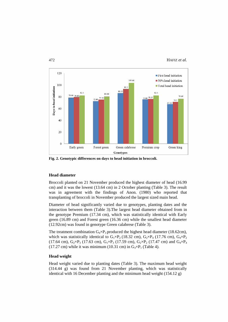
472 HAFIZ et al.
Fig. 2. Genotypic differences on days to head initiation in broccoli.
Head diameter
Broccoli planted on 21 November produced the highest diameter of head (16.99
cm) and it was the lowest (13.64 cm) in 2 October planting (Table 3). The result
was in agreement with the findings of Anon. (1980) who reported that
transplanting of broccoli in November produced the largest sized main head.
Diameter of head significantly varied due to genotypes, planting dates and the
interaction between them (Table 3).The largest head diameter obtained from in
the genotype Premium (17.34 cm), which was statistically identical with Early
green (16.89 cm) and Forest green (16.36 cm) while the smallest head diameter
(12.92cm) was found in genotype Green calabrese (Table 3).
The treatment combination G4×P3 produced the highest head diameter (18.62cm),
which was statistically identical to G1×P2 (18.32 cm), G2×P4 (17.76 cm), G4×P2
(17.64 cm), G2×P3 (17.63 cm), G1×P3 (17.59 cm), G2×P2 (17.47 cm) and G4×P4
(17.27 cm) while it was minimum (10.31 cm) in G3×P1 (Table 4).
Head weight
Head weight varied due to planting dates (Table 3). The maximum head weight
(314.44 g) was found from 21 November planting, which was statistically
identical with 16 December planting and the minimum head weight (154.12 g)
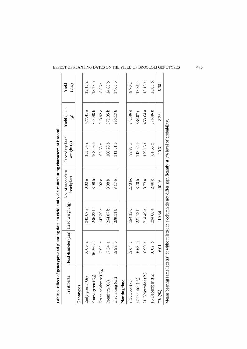
EFFECT OF PLANTING DATES ON THE YIELD OF BROCCOLI GENOTYPES 473
Ta
ble
3.
Eff
ect
of
gen
oty
pes
an
d p
lan
tin
g d
ate
on
yie
ld a
nd
yie
ld c
on
trib
uti
ng
ch
ara
cter
s o
f b
rocc
oli
.
Tre
atm
ents
H
ead
dia
met
er (
cm
) H
ead
wei
ght
(g)
No
. o
f se
cond
ary
hea
d/p
lant
Sec
ond
ary h
ead
wei
ght
(g)
Yie
ld /
pla
nt
(g)
Yie
ld
(t/h
a)
Gen
oty
pes
Ear
ly g
reen
(G
1)
16
.89
a 3
43
.87
a
3.8
3 a
1
33
.54
a
47
7.4
1 a
1
9.1
0 a
Fo
rest
gre
en (
G2)
16
.36
ab
23
6.2
2 b
3
.08
b
10
8.2
6 b
3
44
.48
b
13
.78 b
Gre
en c
alab
rese
(G
3)
12
.92
c 1
47
.39
c
1.9
2 c
6
6.5
3 c
2
13
.92
c
8.5
6 c
Pre
miu
m (
G4)
17
.34
a 2
64
.07
b
3.0
8 b
1
08
.28
b
37
2.3
5 b
1
4.8
9 b
Gre
en k
ing (
G5)
15
.58
b
23
9.1
1 b
3
.17
b
11
1.0
1 b
3
50
.13
b
14
.00 b
Pla
nti
ng
tim
e
2 O
cto
ber
(P
1)
13
.64
c 1
54
.12
c
2.7
3 b
c 8
8.3
5 c
2
42
.46
d
9.7
0 d
27
Oct
ob
er (
P2)
16
.63
b
22
1.1
2 b
3
.20
b
11
2.9
4 b
3
34
.07
c
13
.36 c
21
N
ovem
ber
(P
3)
16
.99
a 3
14
.49
a
3.7
3 a
1
39
.16
a
45
3.6
4 a
1
8.1
5 a
16
Dec
emb
er (
P4)
16
.02
b
29
4.8
0 a
2
.40
c
81
.65 c
3
76
.46
b
15
.06 b
CV
(%
) 6
.01
10
.34
10
.26
10
.31
8.3
8
8.3
8
Mea
ns
bea
rin
g s
am
e le
tter
(s)
or
wit
ho
ut
lett
er i
n a
co
lum
n d
o n
ot
dif
fer
sig
nif
ican
tly a
t 1
% l
evel
of
pro
bab
ilit
y.

474 HAFIZ et al.
Ta
ble
4.
Inte
ract
ion
eff
ect
of
gen
oty
pes
an
d p
lan
tin
g d
ate
s o
n y
ield
an
d y
ield
co
ntr
ibu
tin
g c
ha
ract
ers
of
bro
cco
li.
Inte
ract
ion (
G×
P)
Hea
d d
iam
eter
(cm
)
Hea
d w
eight
(g)
No
. o
f se
cond
ary
hea
d/p
lant
Sec
ond
ary h
ead
wei
ght
(g)
Yie
ld /
pla
nt
(g)
Yie
ld
(t/h
a)
G1×
P1
15
.60 d
e 2
39
.83
ef
3.6
7 a
-c
11
8.2
5 b
-d
35
8.0
8 f
g
14
.32 f
G1×
P2
18
.32 a
4
37
.42
a
4.0
0 a
b
14
0.9
1 a
-c
43
2.4
7 d
e 1
7.3
0 d
G1×
P3
17
.59 a
-c
40
6.6
9 a
b
4.6
7 a
1
73
.48
a
58
0.1
7 a
2
3.2
1 a
G1×
P4
16
.04 b
-e
29
1.5
6 c
-e
3.0
0 b
-e
10
1.5
2 c
-e
53
8.9
4 a
b
21
.56 a
b
G2×
P1
12
.59 g
1
20
.85
ij
2.6
7 b
-e
86
.59 d
-f
20
7.4
4 j
k
8.3
0 j
k
G2×
P2
17
.47 a
-c
25
3.5
2 d
-f
3.3
3 b
-d
11
7.6
5 b
-d
37
1.1
7 e
-g
14
.85 e
f
G2×
P3
17
.63 a
-c
30
3.4
9 c
d
4.0
0 a
b
14
9.0
4 a
b
45
2.5
3 c
d
18
.10 c
d
G2×
P4
17
.76 a
b
26
7.0
1 d
-f
2.3
3 c
-e
79
.77 d
-f
34
6.7
7 f
g
13
.87 f
g
G3×
P1
10
.31 h
1
75
.52
g-i
1
.67
e
56
.65 e
f 1
29
.17
l
5.1
7 l
G3×
P2
13
.82 f
g
12
0.1
3 i
j 2
.00
de
69
.98 e
f 1
92
.11
kl
7.6
8 k
G3×
P3
14
.62 e
f 2
15
.11
f-h
2
.33
c-e
8
7.1
1 d
-f
30
2.2
3 g
i 1
2.0
9 g
h
G3×
P4
12
.95 f
g
76
.79 j
1
.67
e
52
.38 f
2
32
.17
jk
9
.29
i-k
G4×
P1
15
.85 c
-e
16
3.2
5 h
i 2
.67
b-e
8
6.7
3 d
-f
24
9.9
8 i
-k
10
.00 i
j
G4×
P2
17
.64 a
-c
21
1.0
4 f
-h
3.3
3 b
-d
11
8.0
0 b
-d
32
9.0
4 g
h
13
.16 f
g
G4×
P3
18
.62 a
3
52
.12
bc
4.0
0 a
b
14
8.8
2 a
b
50
0.9
3 b
c 2
0.0
4 b
c
G4×
P4
17
.27 a
-d
32
9.8
8 c
2
.33
c-e
7
9.5
6 d
-f
40
9.4
4 d
-f
16
.38 d
e
G5×
P1
13
.83 f
g
16
9.8
7 g
i 3
.00
b-e
9
7.7
8 c
-f
26
7.6
5 h
-j
10
.71 h
i
G5×
P2
15
.90 c
-e
22
7.3
7 f
g
3.3
3 b
-d
11
8.1
7 b
-d
34
5.5
4 f
g
13
.82 f
g
G5×
P3
16
.49 b
-d
29
5.0
1 c
-e
3.6
7 a
-c
13
7.3
4 a
-c
43
2.3
5 c
-e
17
.29 d
G5×
P4
16
.09 b
-e
26
4.2
0 d
-f
2.6
7 b
-e
90
.77 d
-f
35
4.9
6 f
g
14
.20 f
g
CV
(%
) 6
.01
10
.34
10
.26
10
.31
8.3
8
8.3
8
Mea
ns
bea
rin
g s
am
e le
tter
(s)
in a
co
lum
n d
o n
ot
dif
fer
sign
ific
antl
y a
t 5
% l
evel
of
Pro
bab
ilit
y.
G1 =
Ear
ly g
reen
, G
2 =
Fo
rest
gre
en,
G3 =
Gre
en c
alab
rese
, G
4 =
Pre
miu
m c
rop
, G
5 =
Gre
en k
ing a
nd
P1=
2 O
cto
ber
, P
2 =
27 O
cto
ber
, P
3=
21
No
vem
ber
, P
4=
16
Dec
emb
er.

EFFECT OF PLANTING DATES ON THE YIELD OF BROCCOLI GENOTYPES 475
was found from 2 October planting. This result was in agreement with the
findings of Anon. (1977) who reported that planting of broccoli on 28 November
gave the maximum weight of head.
Central head weight was significantly influenced by the genotypes, planting dates
and their interaction effects (Table 3). The maximum weight was recorded from
genotype Early green (343.87 g) followed by Premium (264.07 g) which was
statistically identical with Green king (239.11 g) and Forest green (236.22 g)
while it was minimum (147.39 g) in Green calabrese (Table 3).Genotype Early
green produced the highest head weight might be due to producing higher
number of leaves and head diameter. Srivastava (1960) reported that good head
depends on the number of leaves, their size (length and breadth) and ability to
store carbohydrates and other nutrients within a particular temperature range.
Due to combined effect of genotype and planting dates head weight differed
significantly ranging from 76.79 to 437.42 g (Table 4). The maximum head
weight (437.42 g) was recorded from G1×P2 (Early green planted on 27 October)
that was statistically identical with G1×P3 (406.69 g). The minimum head weight
(76.79 g) was obtained from G3×P4 (Green calabrese planted on 16 December).
The plants of G1P2 and G1P3 performed better might be due to prevailing suitable
temperature for vigorous vegetative growth resulting in higher head weight.
Similar results were obtained by Bianco et al., (1996) who reported that central
head yield was higher when crop planted earlier.
Number of secondary heads per plant
Number of secondary heads per plant also varied significantly due to different
planting dates (Table 3). Number of secondary head of broccoli per plant varied
from 2.40 to 3.73. The maximum number of secondary head per plant (3.73) was
observed on 21 November planting and minimum (2.40) on 16 December
planting.
The secondary head was those, which develop after harvest of main head. The
results revealed that there was a variation in number of secondary heads among
the genotypes (Table 3). Maximum number of secondary heads per plant (3.83)
was recorded in genotype Early green. The minimum number of secondary heads
per plant (1.92) was found in Green calabrese.
A significant variation in number of secondary heads per plant was observed due
to interaction of genotypes and planting dates (Table 4). The maximum number
of secondary heads per plant (4.67) was obtained from G1×P3 (Early green
planted on 21 November) which was statistically identical to G1×P2 (4.00), G2×P3
(4.00), G4×P3 (4.00), G1×P1 (3.67) and G5×P3 (3.67).The minimum number of
secondary heads per plant (1.67) was observed in treatment G3×P1 and G3×P4.

476 HAFIZ et al.
Secondary head weight
Secondary head weight differed significantly among planting dates ranging from
139.16 g to 81.65 g (Table 3). The maximum weight of secondary head (139.16
g) was obtained from 21 November planting which was statistically different to
others, while the minimum (81.65 g) was found from 16 December planting.
There was significant variation on weight of secondary head per plant among the
genotypes (Table 3). The highest weight (133.54 g) of secondary head per plant
was found in Early green and the minimum was in Green calabrese (66.53 g)
while rest of the genotypes produced statistically identical weight of secondary
heads per plant.
The combined effect of genotypes and planting dates was found significant on
secondary head weight (Table 4). The secondary head weight varied from 173.48
to 52.38 g. The maximum head weight (173.48 g) was obtained from treatment
combination G1×P3 (Early green planted on 21 November) which was
statistically identical to G2×P3 (149.04 g), G4×P3 (148.82 g), G1×P2 (140.91 g)
and G5×P3 (137.34 g) while it was the minimum (52.38g) in G3×P4 (Green
calabrese planted at 16 December).
Yield per plant
Yield per plant varied significantly with planting dates (Table 3). The maximum
yield per plant (453.64 g) was found in 21 November planting followed by 16
December (376.46 g) and 27 October planting (334.07 g) whereas it was the
minimum (242.46 g) in 2 October planting.
Genotypes of broccoli differed significantly regarding yield per plant (Table 3).
The genotype Early green produced the maximum yield per plant (477.41 g)
followed by Premium (372.35 g), which was statistically similar to Green king
(350.13 g) and Forest green (344.48 g). The minimum yield per plant (213.92 g)
was found in Green calabrese.
Significant variation was observed in yield per plant due to the interaction of
genotypes and planting dates (Table 4). The highest yield per plant (580.17 g)
was obtained from G1×P3, which was statistically identical to G1×P4 (538.94 g)
followed by G4×P3 (500.93 g) and G2×P3 (452.53 g) while it was minimum
(129.17 g) in G3P1. The treatment combination G1P3 performed the best might be
due to the production of higher number of leaves, head diameter, head weight
and secondary head weight by the genotype Early green in presence of good
environmental condition on 21 November planting.

EFFECT OF PLANTING DATES ON THE YIELD OF BROCCOLI GENOTYPES 477
Total yield
Planting dates also had significant influence on the yield of broccoli (Table 3).
Broccoli of 21 November planting produced the highest yield (18.15 t/ha)
followed by the 16 December planting (15.06 t/ha). It might be due to favorable
low temperature for the head setting and development. On the other hand,
minimum yield (9.70 t/ha) was obtained from 2 October planting. It might be due
to comparatively higher temperature than the optimum at that time.
The total yield of broccoli consisted of the main head and the secondary head
those develop after the removal of the main one. Although the core of stem is
also edible, it is usually not included as part of the yield. Significant variation in
yield (t/ha) was observed among the genotypes (Table 3).The maximum yield
(19.10 t/ha) was obtained from genotype Early green. This might be due to best
performance of this genotype in head diameter, head weight and secondary head
weight. The lowest yield (8.56 t/ha) was recorded from Green calabrese.
Interaction effect of genotypes and planting dates on yield per hectare was found
significant (Table 4). The plants of G1×P3 produced the maximum yield (23.21
t/ha) which was statistically identical to G1×P4 (21.56 t/ha) followed by G4×P3
(20.04 t/ha) while the lowest yield was obtained from G3×P1 (5.17 t/ha).
Conclusion
Considering yield contributing characters and yield potential of Broccoli,
genotype Early green was found the best among the studied genotypes. 21
November was found to be the optimum date of planting for Broccoli. So the
genotypes Early green should be planted on 21 November for maximum yield of
Broccoli.
References
Ahmed, M. S. and A. M. Abdullah. 1986. Effect of time of planting on the yield of
sprouting broccoli. Bangladesh. Hort. 14(2): 47-48.
Ahmed, M. J., Q. Karim and W. Siddique. 2004. Effect of sowing dates on growth and
yield of broccoli (Brassica oleracea var. italica L.) under Rawalakot conditions,
Pakistan. Asian J. Plant Sci. 3(2):167-169.
Anonymous. 1998. Year Book of Agricultural Statistics of Bangladesh, 1996-97.
Bangladesh Bur. of Stat., Govt. People’s Repub. Bangladesh, Dhaka, Bangladesh.
Anonymous. 2004. Annual Report, 2003-04. Bangladesh Agricultural Research Institute,
Gazipur. l.c., 452.
Bianco, V. V.,G. Darnato, R. Pomarici, J. S. Dias, I. Crute and A. A. Monteiro. 1996.
Sowing and transplanting date in four Cima de rapa (Brassica rapa L.) cultivars. I.
sowing dates. Acta Horticulture 407:293-298.

478 HAFIZ et al.
Bose, T. K. and M.G. Som. 1986.Vegetable crops in India.1st
edi. NayaPrakash, Calcutta
6:770-773.
Brammer, H. 1971. Soil resources.Soil survey project, Bangladesh AGL.SF/PAK. 6.
Technical report 3.
Gautam, B. P., A. Shadeque and L. Saikia. 1998. Effect of sowing dates and varieties on
growth and yield of early cauliflower. Journal of Vegetable Science 25(1):1-4.
Prasad, S. and U. Kumer. 1999. Principles of Horticulture. Agrobotanica, 4E 176. J. N.
Vyas Nagar, India. l.c. 6.
Rashid, M. A., A. Shahabuddin, S. N. Mondal, A. K. M. A. Hossaain. 1976. Effect of
time of planting on the performance of some cauliflower varieties. Bangladesh J. of
Agri. Res. 15 (1): 38-41.
Saheed, S. M. 1984. Soils of Bangladesh: General soil type. Soil Resources Development
Institute (SRDI), Dhaka, Bangladesh. P. 3.
Salter, P. J. and R. J. Ward. 1972. Study in crop maturity in cauliflower III. Effect of cold
treatment and certain growth regulators on crop maturity, charecteristics and yield.
J. Hort. Sci. 47(1):57.
Srivastava, R. C. 1960. Three steps to a bumper cauliflower crops. Indian Farming
9(11):8-9.
Toth, N., J. Borosic, I. Zutic, B. Novak, and B. Benko. 2007. Yield components of
broccoli cultivars grown in the continental climate of Croatia. Acta Horticulture 729:
255-260.

ISSN 0258-7122
Bangladesh J. Agril. Res. 40(3): 479-489, September 2015
VARIABILITY, CORRELATION AND PATH ANALYSIS IN PUMPKIN
(Cucurbita moschata L .)
S. SULTANA1, M. A. KAWOCHAR
2, S. NAZNIN
3
A. SIDDIKA4
AND F. MAHMUD5
Abstract
Twenty one genotypes of pumpkin (Cucurbita moschata L.) were evaluated to
measure the variability among the genotypes for several characters, estimate
genetic parameters, association among the characters and their contribution to
yield. There was a great deal of significant variation for all the characters among
the genotypes. High variability was observed in number of female flowers/plant,
number of male flowers/plant, single fruit weight and fruit yield/plant. All the
characters except days to first male flowering and days to first female flowering
showed high heritability along with high genetic advance in percent of mean.
The positive and strong association of number of female flowers/plant (rg=0.918,
rp=0.839), number of male flowers/plant (rg=0.687, rp=0.638), fruit length
(rg=0.691, rp= 0.520), fruit breadth (rg=0.518, rp=0.420) and single fruit weight
(rg=0.492, rp= 0.431) with fruit yield/plant revealed the importance of these
characters in determining fruit yield/plant. On the other hand, days to first male
flowering (rg = -0.623, rp = -0.550) and days to first female flowering (rg= -
0.689, rp= -0.543) correlated significantly and negatively with fruit yield/plant.
The path co-efficient analysis revealed that the highest positive direct effect was
recorded in number of female flowers (0.887) to fruit yield and high direct effect
was found in case of days to first female flowering (0.798). Fruit breadth was
observed to have the highest positive indirect effect (0.899). In case of fruit
length (0.381) and single fruit weight (0.398), the significant positive correlation
with fruit yield/plant was observed because of the combination of the direct and
indirect effects of fruit length and single fruit weight to fruit yield/plant. Overall,
the results indicated that days to first female flowering, number of female
flowers, fruit length, fruit breadth and single fruit weight can be used as useful
selection criteria to increase fruit yield/plant in pumpkin.
Keywords: Pumpkin, variability, Correlation, Path co-efficient analysis.
Introduction
Pumpkin (Cucurbita spp.) is one of the cucurbitaceous fruit vegetables of
Bangladesh. It is an important source of minerals, fibres, vitamins, antioxidants
and phytonutrients (Aruah et al, 2010) and these make the fruit a whole-some
and healthy item for human consumption. Some authors have reported that
1-3Scientific Officer (Plant Breeding), Tuber Crops Research Centre, Bangladesh
Agricultural Research Institute (BARI), Gazipur-1701, 4Scientific Officer, Oilseed
Research Centre, BARI, Gazipur-1701, 5Professor, Department of Genetics and Plant
Breeding, Sher-e-Bangla Agricultural University, Dhaka-1207, Bangladesh.
480 SULTANA et al.
pumpkin fruits possess high medicinal values (Abd El-Aziz and Abd El- Kakek,
2011). Pumpkin seed is an excellent source of protein and has pharmacological
values such as anti-diabetic (Li et al, 2003), antibacterial and antiinflammation
activities (Fu et al, 2006) and antioxidant effects (Nkosi et al., 2006). Despite its
health and dietary benefits, the production of pumpkin in Bangladesh is mostly
done on a small scale with low yield. The total production of pumpkin was 0.218
million tons in 2011 in this country (BBS, 2011). However, cultivation of this
crop is highly desirable to overcome the problems of under-nourishment and
food poverty in Bangladesh. A large number of pumpkin genotypes are cultivated
in Bangladesh but no serious attempts have been made to improve its
productivity and acceptability.
The success of any crop improvement program depends, to a large extent, on the
amount of genetic variability present in the population. Intensive research efforts
are needed in several areas particularly in selection of superior pumpkin
genotypes. There is a wide genetic variability among the existing genotypes (Aliu
et al, 2011) and thus, the utilization of such variability in the breeding programs
of this crop is possible. In a crop selection program, knowledge of the
interrelationships among yield and yield contributing characters are necessary.
Path analysis would help in partitioning the correlation coefficient into direct and
indirect effects of various traits on the genetic variability, character association
and the direct and indirect contributions of some yield characters towards fruit
yield. Thus, the present investigation was undertaken with the view to estimate
variability and character association in pumpkin.
Materials and Method
The investigation was carried out at the experimental field of Sher-e-Bangla
Agricultural University, Dhaka, Bangladesh during the period from March to
August 2010 to study the variability and character association in 21 pumpkin
genotypes. The experiment was laid out in Randomized Complete Block
Design (RCBD) with three replications. These genotypes were assigned at
random into pits of each replication. Pits of 55 cm x 55 cm x 50 cm were
prepared in each block at a spacing of 3 m x 3 m. Standard production package
was followed for raising a healthy crop. For studying different genetic parameters
and inter-relationships, thirteen characters were taken into consideration namely,
leaf length, leaf breadth, internodes distance, days to first male flowering, days
to first female flowering, pedicel length of male flower, pedicel length of female
flower, number of male and female flowers/plant, fruit length, fruit breadth, single
fruit weight and fruit yield plant-1
. Analysis of variance (ANOVA), mean and
range were calculated by using MSTATC software program. Phenotypic and
genotypic variances were estimated by the formula given by Johnson et al,
(1955). Genotypic and phenotypic co-efficients of variations were calculated

VARIABILITY, CORRELATION AND PATH ANALYSIS IN PUMPKIN 481
using the formula of Burton (1952) and the values were categorized as low (0-
10%), moderate(10-20%) and high (20% and above) as suggested by
Shivasubramanian and Menon (1973). Heritability was measured using the
formula given by Singh and Chaudhary, (1985) and the percentage was
categorized as low (0-30%), moderate (30-60%) and high (60% and above) as
given by Robinson et al, (1949). Genetic advance in percentage of mean was
calculated by the formula given by Johnson et al, (1955), and the values were
categorized as low (0-10%), moderate (10-20%) and high (20% and above) as
given by him. Genotypic and phenotypic correlation coefficients were obtained
using the formula suggested by Miller et a,. (1958), and path co-efficient analysis
was done following the method outlined by Dewey and Lu (1959).
Results and Discussion
Genetic Variability: Variance components, genotypic and phenotypic
coefficients of variations, heritability, genetic advance and genetic advance in
percent of mean (GAPM) are presented in Table 1. The phenotypic variance and
phenotypic coefficient of variation were higher than the corresponding genotypic
variance and genotypic coefficient of variation for all the characters under study
suggesting the presence of environmental influence to some extent in the
expressions of these characters. The highest genotypic variance (57.87) as well as
phenotypic variance (85.62) was found in fruit length followed by days to first
male flowering and days to first female flowering. Saha et al, (1992) also found
high genotypic variance (30.34) and phenotypic variance (31.76) in fruit length.
The difference between genotypic variance and phenotypic variance was the
minimum in single fruit weight indicating that less influence of environment on
this character. The highest genotypic (45.76) and phenotypic co-efficients of
variation (69.78) were found in number of female flowers/plant, which indicated
that the genotypes were highly variable for this trait. High variability was also
observed in internode distance, pedicel length of male flower, pedicel length of
female flower, number of male flowers/plant, single fruit weight and fruit
yield/plant. All the characters except days to first male flowering and days to first
female flowering showed high heritability along with high genetic advance in
percent of mean. High heritability estimates for the characters like pedicel length
of male flower (96.49), pedicel length of female flower (95.94), single fruit
weight (81.20) and fruit yield/plant. On the other hand, genetic advance for these
characters were 71.39, 82.02, 65.55 and 106.73, respectively. Chowdhury and
Sharma (2002) found high values of heritability, PCV, GCV and genetic advance
for yield/ha and single fruit weight. High heritability with high genetic advance in
percent of mean indicated that the character is mostly governed by additive
genes, and selection based on this character would be effective for future
breeding program.

482 SULTANA et al.
Ta
ble
1.
Est
ima
tio
n o
f so
me
gen
etic
pa
ram
eter
s in
21
gen
oty
pes
of
pu
mp
kin
.
Par
amet
ers
p
g
P
CV
G
CV
H
erit
abil
ity
(%)
Gen
etic
ad
vance
Gen
etic
ad
vance
(%
mea
n)
Lea
f le
ngth
wit
ho
ut
pet
iole
(cm
) 8
.71
7.9
0
17
.16
16
.34
90
.70
5
.51
32
.03
Lea
f b
read
th a
t th
e m
axim
um
wid
th (
cm
) 1
3.5
8
12
.37
15
.76
15
.04
91
.12
6
.92
29
.59
Inte
rno
des
dis
tance
1
2.6
1
8.2
5
25
.06
20
.27
65
.43
4
.79
33
.80
Days
to f
irst
mal
e fl
ow
erin
g
62
.30
44
.07
11
.21
9.4
3
70
.74
1
1.5
0
16
.34
Days
to f
irst
fem
ale
flo
wer
ing
5
5.9
0
39
.96
9.9
5
8.4
1
71
.50
1
1.0
1
14
.65
Ped
icel
len
gth
of
male
flo
wer
(cm
) 3
5.8
6
34
.60
35
.91
35
.28
96
.49
1
1.9
0
71
.39
Ped
icel
len
gth
of
fem
ale
flo
wer
(cm
) 3
.41
3.2
7
41
.42
40
.57
95
.94
3
.65
82
.02
Nu
mb
er o
f m
ale
flo
wer
s/p
lant
17
.31
11
.82
61
.38
50
.72
68
.28
5
.85
86
.41
Nu
mb
er o
f fe
mal
e fl
ow
ers/
pla
nt
6.1
0
2.6
2
69
.78
45
.76
43
.00
2
.19
62
.04
Fru
it l
eng
th (
cm
) 8
5.6
2
57
.87
17
.35
14
.26
67
.59
1
2.8
8
24
.15
Fru
it b
read
th (
cm
) 2
6.9
0
19
.23
18
.79
15
.89
71
.47
7
.64
27
.69
Sin
gle
fru
it w
eig
ht
(kg)
0.6
7
0.5
5
39
.26
35
.38
81
.20
1
.37
65
.55
Fru
it y
ield
/pla
nt
(kg)
8.7
3
6.1
4
73
.53
61
.64
70
.27
4
.28
10
6.7
3
2 p
= P
hen
oty
pic
var
iance
,
2g =
Gen
oty
pic
var
iance
, P
CV
= P
hen
oty
pic
co
effi
cient
of
var
iati
on,
GC
V =
Gen
oty
pic
co
effi
cien
t o
f
var
iati
on.

VARIABILITY, CORRELATION AND PATH ANALYSIS IN PUMPKIN 483
High heritability and moderate genetic advance in percent of mean found in days
to first male flowering (70.74, 16.34) and days to first female flowering (71.50,
14.65) indicated the non-additive gene effect. Therefore, high heritability does
not necessarily mean that the character will show high genetic advance. Selection
based upon phenotypic expression of these characters would not be effective for
the improvement of this crop. Singh and Lal (2005) reported similar results.
Correlation co-efficient: Correlation studies have been done both at phenotypic
and genotypic level and showed that genotypic correlation was higheer than the
respective phenotypic correlation in most of the cases suggesting strong inherent
association between the characters under study (Table 2). Similar result was
found by Pankaj et al, (2002). Lower phenotypic correlation coefficients than
genotypic correlation coefficients indicate that both environmental and genotypic
correlations in those cases act in same direction, and finally maximize their
expression at phenotypic level.
In present investigation, number of female flowers/plant gave the highest
significant positive association with fruit yield/plant (rg=0.918, rp=0.839). In
addition, fruit yield/plant was also correlated positively and significantly with
number of male flowers (rg=0.687, rp= 0.638). This means that increase in the
number of male and female flowers would result in higher pollen production and
therefore, enhance fertilization and ultimately fruit yield/plant. Shah and Kale
(2002) reported close association and dependency of yield with number of female
flowers.
A significant positive correlation was also obtained between number of male
flowers and number of female flowers (rg = 0.852, rp = 0.769). This suggests that
the number of male and female flowers increases or decreases simultaneously,
and these could be linked to enhance pollination efficiency in the plant. Positive
genetic correlation was reported between the number of male and female flowers
in pumpkin (Aruah et al., 2012)
On the other hand, the number of male flowers was correlated significantly and
negatively with days to first male flowering (rg = -0.597, rp = -0.410) and days to
first female flowering (rg = -0.443, rp = -0.329). Similar result was found in case
of number of female flowers. These results indicated that early flowering
increased the number of male and female flowers and increased number of male
and female flowers which increased yield/plant. This result was in agreement
with Mohanty (2001) who reported that early flowering at lower nodes and
higher number of flowers/plant, particularly the female flower, increase fruit
yield. Badade et al, (2001) found negative association of yield/ vine with days to
first male flower opening.
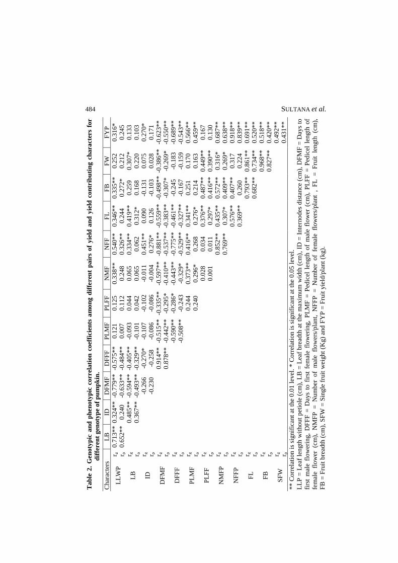
484 SULTANA et al.
Ta
ble
2.
Gen
oty
pic
an
d p
hen
oty
pic
co
rrel
ati
on
co
effi
cien
ts a
mo
ng
dif
fere
nt
pa
irs
of
yie
ld a
nd
yie
ld c
on
trib
uti
ng
ch
ara
cter
s fo
r
dif
feren
t g
eno
typ
e o
f p
um
pk
in.
Char
acte
rs
L
B
ID
DF
MF
D
FF
F
PL
MF
P
LF
F
NM
F
NF
F
FL
F
B
FW
F
YP
LL
WP
r g
0
.71
3** 0
.32
4**
-0.7
79
**
-0
.57
5**
0
.12
1
0.1
25
0.3
38
**
0.5
40
**
0.3
46
**
0.3
35
**
0.2
52
0.3
16
*
r p
0.6
52
**
0.2
40
-0.6
33
**
-0
.48
4**
0
.00
7
0.1
12
0.2
48
0.3
26
**
0.2
44
0.2
72
*
0.2
12
0.2
45
LB
r g
0.4
85
**
-0.5
94
**
-0
.40
5**
-0
.09
3
0.0
44
0.0
65
0.3
34
**
0.4
19
**
0.2
59
0.3
07
*
0.1
33
r p
0.3
67
**
-0.4
93
**
-0
.32
9**
-0
.10
1
0.0
42
0.0
65
0.0
62
0.3
12
*
0.1
68
0.2
20
0.1
03
ID
r g
-0.2
66
-0
.27
0*
-0.1
07
-0.1
02
-0.0
11
0.4
51
**
0.0
90
-0.1
31
0.0
75
0.2
70
*
r p
-0.2
30
-0
.25
8
-0.0
86
-0.0
86
-0.0
04
0.2
76
*
0.1
26
-0.1
03
0.0
28
0.1
71
DF
MF
r g
0.9
14
**
-0.5
15
**
-0
.33
5**
-0
.59
7**
-0
.88
1**
-0
.55
9**
-0
.49
8**
-0
.38
6**
-0
.62
3**
r p
0.8
78
**
-0.4
42
**
-0
.29
5*
-0.4
10
**
-0
.53
7**
-0
.38
3**
-0
.30
7*
-0.2
69
*
-0.5
50
**
DF
FF
r g
-0
.59
0**
-0
.28
6*
-0.4
43
**
-0
.77
5**
-0
.46
1**
-0
.24
5
-0.1
83
-0.6
89
**
r p
-0
.50
8**
-0
.24
3
-0.3
29
*
-0.5
29
**
-0
.32
7**
-0
.16
7
-0.1
59
-0.5
43
**
PL
MF
r g
0.2
44
0.3
73
**
0.4
16
**
0.3
41
**
0.2
51
0.1
70
0.5
66
**
r p
0.2
40
0.2
96
*
0.2
68
0.2
76
*
0.2
14
0.1
63
0.4
59
**
PL
FF
r g
0
.02
8
0.0
34
0.3
76
**
0.4
87
**
0.4
49
**
0.1
67
r p
0
.00
1
0.0
11
0.2
97
*
0.4
16
**
0.3
90
**
0.1
30
NM
FP
r g
0.8
52
**
0.4
35
**
0.5
72
**
0.3
16
*
0.6
87
**
r p
0.7
69
**
0.3
07
*
0.4
09
**
0.2
69
*
0.6
38
**
NF
FP
r g
0
.57
6**
0.4
07
**
0.3
17
0.9
18
**
r p
0
.36
9**
0.2
60
0.2
24
0.8
39
**
FL
r g
0.7
93
**
0.8
61
**
0.6
91
**
r p
0.6
82
**
0.7
34
**
0.5
20
**
FB
r g
0
.96
8**
0.5
18
**
r p
0
.82
7**
0.4
20
**
SF
W
r g
0
.49
2**
r p
0.4
31
**
** C
orr
elat
ion i
s si
gnif
icant
at t
he
0.0
1 l
evel
. * C
orr
elat
ion i
s si
gnif
icant
at t
he
0.0
5 l
evel
.
LL
P =
Lea
f le
ngth
wit
ho
ut
pet
iole
(cm
), L
B =
Lea
f b
read
th a
t th
e m
axim
um
wid
th (
cm
), I
D =
Inte
rno
des
dis
tance
(cm
), D
FM
F =
Days
to
firs
t m
ale f
low
erin
g,
DF
FF
= D
ays
to f
irst
fem
ale
flo
wer
ing,
PL
MF
= P
edic
el l
eng
th o
f m
ale
flo
wer
(cm
), P
LF
F =
Ped
icel
len
gth
of
fem
ale
flo
wer
(c
m),
N
MF
P =
N
um
ber
o
f m
ale
flo
wer
s/p
lant,
N
FF
P =
N
um
ber
o
f fe
mal
e fl
ow
ers/
pla
nt
, F
L =
F
ruit
le
ngth
(c
m),
FB
= F
ruit
bre
adth
(cm
), S
FW
= S
ingle
fru
it w
eigh
t (K
g)
and
FY
P =
Fru
it y
ield
/pla
nt
(kg).
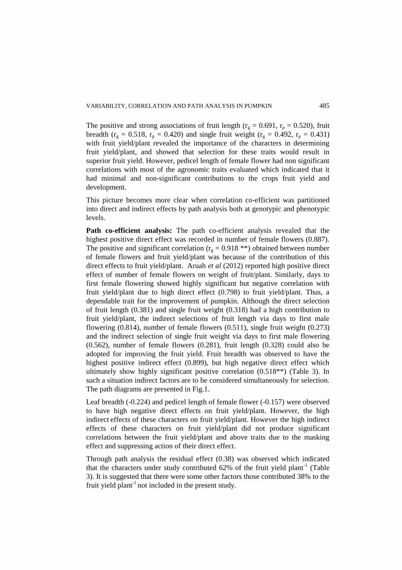
VARIABILITY, CORRELATION AND PATH ANALYSIS IN PUMPKIN 485
The positive and strong associations of fruit length (rg = 0.691, rp = 0.520), fruit
breadth (rg = 0.518, rp = 0.420) and single fruit weight (rg = 0.492, rp = 0.431)
with fruit yield/plant revealed the importance of the characters in determining
fruit yield/plant, and showed that selection for these traits would result in
superior fruit yield. However, pedicel length of female flower had non significant
correlations with most of the agronomic traits evaluated which indicated that it
had minimal and non-significant contributions to the crops fruit yield and
development.
This picture becomes more clear when correlation co-efficient was partitioned
into direct and indirect effects by path analysis both at genotypic and phenotypic
levels.
Path co-efficient analysis: The path co-efficient analysis revealed that the
highest positive direct effect was recorded in number of female flowers (0.887).
The positive and significant correlation (rg = 0.918 **) obtained between number
of female flowers and fruit yield/plant was because of the contribution of this
direct effects to fruit yield/plant. Aruah et al (2012) reported high positive direct
effect of number of female flowers on weight of fruit/plant. Similarly, days to
first female flowering showed highly significant but negative correlation with
fruit yield/plant due to high direct effect (0.798) to fruit yield/plant. Thus, a
dependable trait for the improvement of pumpkin. Although the direct selection
of fruit length (0.381) and single fruit weight (0.318) had a high contribution to
fruit yield/plant, the indirect selections of fruit length via days to first male
flowering (0.814), number of female flowers (0.511), single fruit weight (0.273)
and the indirect selection of single fruit weight via days to first male flowering
(0.562), number of female flowers (0.281), fruit length (0.328) could also be
adopted for improving the fruit yield. Fruit breadth was observed to have the
highest positive indirect effect (0.899), but high negative direct effect which
ultimately show highly significant positive correlation (0.518**) (Table 3). In
such a situation indirect factors are to be considered simultaneously for selection.
The path diagrams are presented in Fig.1.
Leaf breadth (-0.224) and pedicel length of female flower (-0.157) were observed
to have high negative direct effects on fruit yield/plant. However, the high
indirect effects of these characters on fruit yield/plant. However the high indirect
effects of these characters on fruit yield/plant
did not produce significant
correlations between the fruit yield/plant and above traits due to the masking
effect and suppressing action of their direct effect.
Through path analysis the residual effect (0.38) was observed which indicated
that the characters under study contributed 62% of the fruit yield plant-1
(Table
3). It is suggested that there were some other factors those contributed 38% to the
fruit yield plant-1
not included in the present study.
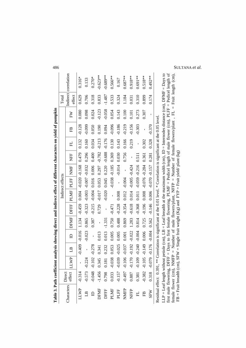
486 SULTANA et al.
Ta
ble
3.
Pa
th c
oef
fici
ent
an
aly
sis
sho
win
g d
irec
t a
nd
in
dir
ect
eff
ect
of
dif
feren
t ch
ara
cter
s o
n y
ield
of
pu
mp
kin
Char
acte
rs
Dir
ect
effe
ct
Ind
irec
t ef
fects
T
ota
l
Ind
irec
t
effe
ct
corr
elat
ion
LL
WP
L
B
ID
DF
MF
D
FF
F
PL
MF
P
LF
F
NM
F
NF
F
FL
F
B
FW
LL
WP
-0
.31
4
- -0
.40
9
-0.0
16
1
.13
4
-0.4
59
0.0
04
-0.0
20 -
0.1
68
0.4
79
0
.13
2
-0.1
28
0.0
80
0.6
29
0.3
16
*
LB
-0
.57
3
-0.2
24
- -0
.02
3
0.8
65
-0.3
23
-0.0
03
-0.0
07 -
0.0
32
0.2
96
0
.16
0
-0.0
99
0.0
98
0.7
06
0.1
33
ID
-0.0
48
-0.1
02
-0.2
78
- 0
.38
7
-0.2
15
-0.0
04
0.0
16
0.0
06
0.4
00
0
.03
4
0.0
50
0.0
24
0.3
18
0.2
70
*
DF
MF
-1
.45
6
0.3
45
0.3
41
0.0
13
-
0.7
29
-0.0
17
0.0
53
0.2
97
-0.7
82
-0
.21
3
0.1
90
-0.1
23
0.8
33
-0.6
23
**
DF
FF
0
.79
8
0.1
81
0.2
32
0.0
13
-1
.33
1
- -0
.02
0
0.0
45
0.2
20
-0.6
88
-0
.17
6
0.0
94
-0.0
58
-1.4
87
-0.6
89
**
PL
MF
0
.03
3
-0.0
38
0.0
53
0.0
05
0
.75
0
-0.4
71
- -0
.03
8 -
0.1
85
0.3
69
0
.13
0
-0.0
96
0.0
54
0.5
33
0.5
66
**
PL
FF
-0
.15
7
-0.0
39
-0.0
25
0.0
05
0
.48
8
-0.2
28
0.0
08
- -0
.01
4
0.0
30
0
.14
3
-0.1
86
0.1
43
0.3
24
0.1
67
NM
FP
-0
.49
7
-0.1
06
-0.0
37
0.0
01
0
.86
9
-0.3
54
0.0
12
-0.0
04
- 0
.75
6
0.1
66
-0.2
19
0.1
00
1.1
84
0.6
87
**
NF
FP
0
.88
7
-0.1
70
-0.1
92
-0.0
22
1
.28
3
-0.6
18
0.0
14
-0.0
05 -
0.4
24
- 0
.21
9
-0.1
56
0.1
01
0.0
31
0.9
18
**
FL
0
.38
1
-0.1
09
-0.2
40
-0.0
04
0
.81
4
-0.3
68
0.0
11
-0.0
59 -
0.2
16
0.5
11
-
-0.3
03
0.2
73
0.3
10
0.6
91
**
FB
-0
.38
2
-0.1
05
-0.1
49
0.0
06
0
.72
5
-0.1
96
0.0
08
-0.0
76 -
0.2
84
0.3
61
0
.30
2
- 0
.30
7
0.8
99
0.5
18
**
SF
W
0.3
18
-0.0
79
-0.1
76
-0.0
04
0
.56
2
-0.1
46
0.0
06
-0.0
70 -
0.1
57
0.2
81
0
.32
8
-0.3
70
- 0
.17
4
0.4
92
**
Res
idual
eff
ect:
0
.39
1,
** C
orr
elat
ion i
s si
gn
ific
ant
at t
he
0.0
1 l
evel
. * C
orr
elat
ion i
s si
gnif
icant
at t
he
0.0
5 l
evel
.
LL
P =
Lea
f le
ngth
wit
ho
ut
pet
iole
(cm
), L
B =
Lea
f b
read
th a
t th
e m
axim
um
wid
th (
cm
), I
D =
Inte
rno
des
dis
tance
(cm
), D
FM
F =
Days
to
firs
t m
ale f
low
erin
g,
DF
FF
= D
ays
to f
irst
fem
ale
flo
wer
ing,
PL
MF
= P
edic
el l
eng
th o
f m
ale
flo
wer
(cm
), P
LF
F =
Ped
icel
len
gth
of
fem
ale
flo
wer
(c
m),
N
MF
P =
N
um
ber
o
f m
ale
flo
wer
s/p
lant,
N
FF
P =
N
um
ber
o
f fe
mal
e fl
ow
ers/
pla
nt
, F
L =
F
ruit
le
ngth
(c
m),
FB
= F
ruit
bre
adth
(cm
), S
FW
= S
ingle
fru
it w
eig
ht
(Kg)
and
F
YP
= F
ruit
yie
ld/
pla
nt
(kg)
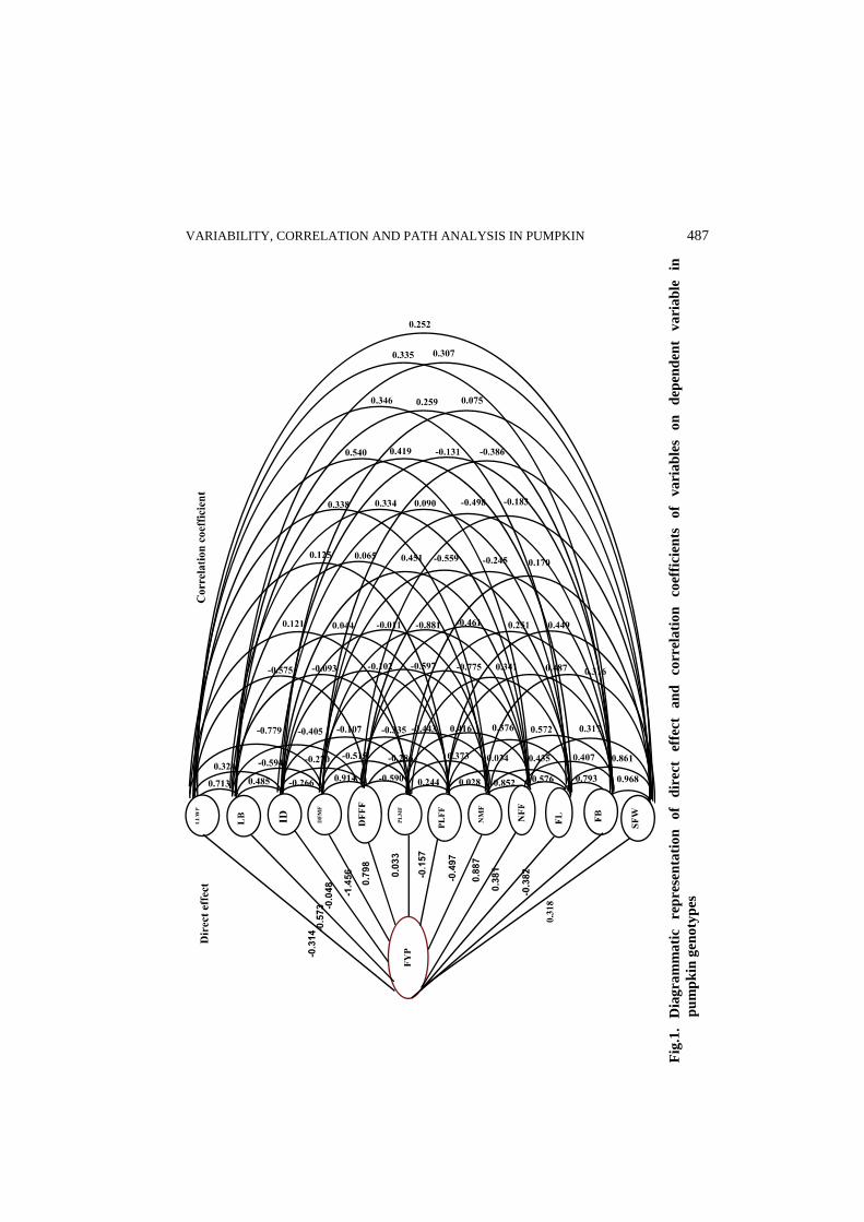
VARIABILITY, CORRELATION AND PATH ANALYSIS IN PUMPKIN 487
Fig
.1.
Dia
gra
mm
ati
c re
pre
sen
tati
on
o
f d
irec
t ef
fect
an
d
corr
ela
tio
n
coef
fici
ents
o
f va
ria
ble
s o
n
dep
end
ent
va
ria
ble
in
pu
mp
kin
gen
oty
pes
488 SULTANA et al.
Wide genetic variability was found among the genotypes. After analyzing the
data obtained from genotypic co-efficient of variation, phenotypic co-efficient of
variation, heritability, genetic advance in percent of mean, correlation coefficient
and path co-efficient analysis, it can be concluded that days to first female
flowering, number of female flowers, fruit length, fruit breadth and single fruit
weight can be used as selection criteria to increase fruit yield/plant in pumpkin.
References
Abd El-Aziz, A. B. and H.H. Abd El-Kalek. 2011. Antimicrobial proteins and oil seeds
from pumpkin (Cucurbita moschata). Nature and Science 9(3): 105-119.
Aliu, S., A. Haziri, S. Fetahu, N. Aliage, I. Rusinove, I. Haziri and V. Arapi. 2011.
Morphological and nutritive variation in a collection of Cucurbita pepo L. growing
in Kosova. Notulae Scientia Biologicae 3(2): 119-122.
Aruah, C. B., M. I. Uguru and B.C. Oyiga . 2010. Nutritional evaluation of some
Nigerian pumpkins (Cucurbita spp.) Fruit, vegetable and Cereal Science and
Biotechnology 5 (Special Issue 2): 64-71
Aruah, C. B., M. I. Uguru, and B.C. Oyiga. 2012. Genetic Variability and Inter-
Relationship among some Nigerian Pumpkin Accessions ( Cucurbita spp.).
International Journal of Plant Breeding 6(1): 34-41.
Badade, D.S., S. D. Warade and S.K. Gaikwad. 2001. Correlation studies in bottle gourd
(Lageneria sicereria (Mol.) Stand). Journal of Maharashtra Agricultural
Universities 26(1):20-22.
BBS. (Bangladesh Bureau of Statistics). 2011. Statistical Year Book of Bangladesh 2010-
2011. Bangladesh Bureau of Statistics Division, Ministry of Planning, Govt.of the
people’s Republic of Bangladesh, Dhaka.
Burton, G.W. 1952. Quantitative inheritance in grasses. Proceeding 6th International
Grassland Congress, Pennsylvania. 17-23 August. Pennsylvania State College, State
College, Pennsylvania, USA. P. 277-283.
Chowdhury, D. and K. C. Sharma. 2002. Studies on variability, heritability, genetic
advance and correlation in ridge gourd (Luffa acutangula Roxb.). Hort. J. 15(3):
53-58.
Dewey, D.R. and K. H. Lu. 1959. A correlation and path coefficient analysis of
components of crested wheat grass seed production. Agron. J. 51:515-518.
Fu, C-L., S.H. Huan, Q.H. Li. 2006. A Review on pharmacological activities and
utilization technologies of pumpkin. Plant Foods for Human Nutrition Journal 61:
70-77
Johnson, H.W., H.F. Rabinson, and R.E. Comstock. 1955. Estimation of genetic and
environmental variability in soybean. Agron. J. 47:314-318.
Li Q-H, Z. Tian, T-Y Cai. 2003. Study on the hypoglycemic action of pumpkin extract in
diabetic rats. Acta Nutrimental Sinica 25: 34-36.

VARIABILITY, CORRELATION AND PATH ANALYSIS IN PUMPKIN 489
Miller, P.A., J.G. Williams, H.F. Robinson, and R.E. Comstock. 1958. Estimates of
genotypic and environmental variances and co-variances in upland cotton and their
implication in selections. Agron. J. 501:126-131.
Mohanty, B. K. 2001. Studies on correlation and path analysis in pumpkin (Cucurbita
moschata). Haryana J. Hort. Sci. 30(1/2): 86-89.
Nkosi C.Z., A.R. Opoku, S.E. Terblanche. 2006. Antioxidant effects of pumpkin seeds
(Cucurbita pepo) protein isolate in CCI-induced liver injury in low-protein fed rats.
Phototherapy Research 20: 935-940.
Pankaj, S., T. Gyanendra, A.S. Gontia, V.D. Patil, and P. Shah. 2002. Correlation
studies in Indian Mustard. Agricultural Science Digest 22(2):79-82.
Robinson, H. I., R. E. Comstock, and P. H. Harvey. 1949. Estimation of heritability and
degree of dominance in corn. Agron. J. 41:353-359.
Saha, R. R., B. N. Mitra, A. E. Hossain, M. Jamaluddin and A. M. M. Mosiul Hoque.
1992. Genetic variability, character association and path coefficient analysis in
pumpkin (Cucurbita moschata L.). Bangladesh Hort., 20(1), 59-62.
Shah, S.R. and P.N. Kale. 2002. Yield component association analysis in ridge gourd.
J. Maharashtra Agril. Univ., 27(2): 197-198.
Shivasubramanian, S. and M. Menon. 1973. Heterosis and inbreeding depression in rice.
The Madras Agricultural Journal 6:1139-1140.
Singh, G. and T. Lal. 2005. Genetic variability, heritability and genetic advance for yield
and its contributing traits in muskmelon (Cucumis melo L.). J. Res. Punjab Agric.
Univ. 42(2): 168-174.
Singh, R.K. and B.D. Chaudhury. 1985. Biometrical Methods in Quantitative Genetic
Analysis. Kalyani Publishers, New Delhi, India. p.56.
Ushakumari, R.M., M. Subramanian, and Subramaniam. 1991. Studies on coefficient of
variation and heritable components of some quantitative characters of Brinjal.
Indian Journal of Horticulture 48(1):75-78.

490 SULTANA et al.
ISSN 0258-7122
Bangladesh J. Agril. Res. 40(3): 491-500, September 2015
EFFECT OF SOWING DATE AND PLANT SPACING ON
SEED PRODUCTION OF CAULIFLOWER
M. F. HOSSAIN1, N. ARA
2, M. R. UDDIN
3
M. R. ISLAM4 AND M. G. AZAM
5
Abstract
The experiment was conducted at Regional Agricultural Research Station,
Ishurdi, Pabna during rabi season of 2011-2012 and 2012-2013 to find out the
appropriate sowing date and optimum plant spacing for seed production of
cauliflower (var. BARI Phulcopi-1). Four sowing dates viz. 20 September, 1
October, 10 October and 20 October and three plant spacing viz. 60 cm × 50 cm,
60 cm × 60 cm and 60 cm × 70 cm were used as treatment variables. Significant
variation in seed yield and yield contributing characters of cauliflower were
observed due to execution of different sowing dates and plant spacing. Number
of branches plant-1
, number of pods plant-1
and number of seeds pod-1
showed
the highest in 1 October sowing as a result the highest seed yield (361.69 kgha-1
)
was obtained from same date of sowing. Sowing on 10 October and 20 October
reduced seed yield drastically compared to that obtained from 1 October sowing.
The lowest seed yield (188.54 kgha-1
) was obtained from 20 October sowing.
On the contrary, closer spacing (60 cm × 50 cm) produced the highest seed yield
(315.88 kgha-1
) and the wider spacing (60 cm × 70 cm) produced the lowest
seed yield (254.07 kgha-1
). However, combination of 1 October sowing with 60
cm × 50 cm plant spacing produced the highest seed yield (414.81 kgha-1
) due to
higher number of seeds pod-1
. The seed yield decreased after 10 October sowing
irrespective of plant spacing. So, early sowing (1 October) with closer spacing
(60 cm× 50 cm) would be economically profitable for cauliflower seed
production in North-Western part of Bangladesh.
Keywords: Cauliflower, sowing, spacing, yield and seed.
Introduction
Cauliflower (Brassica oleracea var. botrytis L.) is a biannual and herbaceous
vegetable crop belonging to the family Cruciferae. It is one of the popular winter
vegetables in Bangladesh. Cauliflower thrives best in a cool moist climate and it
does not withstand very low temperature or too much heat (Din et al., 2007). The
temperature in the country remains higher up to mid October after which
gradually comes down in mid-December and extends up to mid-February. The
1Senior Scientific Officer, Bangladesh Agricultural Research Institute, RARS, Ishwardi,
Pabna, 2Principal Scientific Officer, Bangladesh Agricultural Research Institute, Gazipur,
3Principal Scientific Officer, Bangladesh Agricultural Research Institute, RARS,
Ishwardi, Pabna, 4Senior Scientific Officer, Bangladesh Agricultural Research Institute,
RARS, Ishwardi, Pabna, 5Scientific Officer, Bangladesh Agricultural Research Institute,
PRC, Ishwardi, Pabna, Bangladesh.
492 HOSSAIN et al.
temperature increases sharply thereafter. Optimum plant spacing is important for
crop production through efficient utilization of light, nutrients and water by the
plants. In some cases higher plant population adversely affect yield per unit area
hampering vegetative and reproductive growth of plant specially head size and
delay in seed maturity. So, it is essential to maintain optimum plant spacing for
maximum seed yield of cauliflower. Baloch (1994) recommended that relatively
wide spacing (60 cm × 60 cm) promotes earliness and larger heads, but yield and
number of curds usually increased by close spacing (45 cm × 45 cm). Increase
the plant density limits the availability of space for lateral growth, resulting in
increase in plant height (Pandita et al., 2005). Seeds of cauliflower are produced
in the country in a small scale but the maximum amount of seeds of cauliflower
is imported from other countries. The meteorological data for the last 10 years
indicated that the crop suffer from cold injury during the month of January
(Anon, 2007) which resulted low yield of crop. The optimum temperature for
cauliflower withstands is 10 to 150C (Din et al., 2007) but in the north-western
part of the country, the night temperature falls even below 5-60C which affects
crop yield loss. Early sowing recorded maximum vegetative growth and higher
yield than late planting (Alam et al., 2010). Lavanya et al., (2014) recommended
that early sowing (1st October) with closer spacing is suitable treatment
combination for higher seed yield of radish. So, it is needed to optimize sowing
date for quality seed production of cauliflower. Keeping in view, the present
experiment was conducted to find out the suitable sowing date and determine the
optimum plant spacing for seed production of cauliflower.
Materials and Method
The experiment was carried out at Regional Agricultural Research Station,
Ishurdi, Pabna during rabi season of 2011-12 and 2012-13. The initial soil
samples were collected from the experimental field for a depth of 0-15 cmprior to
application of fertilizers. The nutrient status of soil of the experimental plot was
determined at the Soil Science Lab of Soil Science Division, Bangladesh
Agricultural Research Institute, Joydebpur, Gazipur. Results of soil analysis are
presented in Table 1. Four sowing dates viz. 20 September, 1 October, 10
October and 20 October and three plant spacing viz. 60 cm × 50 cm, 60 cm × 60
cm and 60 cm × 70 cm were used as treatment variables. The treatments were
factorial combination of the two factors and the experiment was conducted using
a randomized complete block design with three replications. The unit plot size
was 10 m ×1.2 m. Seeds of variety BARI Phulcopi-1 were sown in the nursery
beds at an interval of 10 days started from 20 September. Beds were immediately
irrigated with the help of watering cane. After germination, when the seedlings
were attained at a height of 3 cm then the seedlings were transplanted in the
other nursery beds 10 cm apart for proper growth and development of the
seedlings. Thirty days old seedlings were transplanted in the evening time in the

EFFECT OF SOWING DATE AND PLANT SPACING ON SEED 493
experimental plot according to the treatment. Healthy seedlings of uniform size
were selected for planting. Before transplantation, the nursery beds were irrigated
so that the seedlings could be easily uprooted from the beds without any damage
of the root. After one week of transplantation, dead seedlings were replaced by
planting fresh seedlings to obtain a uniform stand. The land was fertilized with
well decomposed cowdung @ 15 tha-1
and 120, 55, 100, 15 1.5, 2 and 1 kgha-1
N
P K S B Zn and Mo, respectively as a source of Urea, TSP, MoP, Gypsum, Boric
acid, Zinc sulphate and Sodium molybdate, respectively. Curds with hollow stem
disorder is a major problem in cauliflower production and is associated with Mo
deficiency. So, Mo application is a crucial factor for yield and quality as well as
to control curds with hollow stem disorder. Total amount of cow dung, TSP,
gypsum, zinc sulphate, boric acid and sodium molybdate were applied in the plot
during final land preparation. Urea and MoP were applied in four equal
installments at 20, 40, 60 and 90 days after planting. After transplantation, the
experimental plot was irrigated by watering cane and second irrigation (flood
irrigation) was done 3 days after transplantation. After this, irrigations were done
after fertilizer application and as and when required. Three weeding were done
for weed control at 20, 40 and 60 DAT. In the early stage of transplantation
damping off disease was occurred in early sowing but serious in late sowing and
it was controlled by spraying Bavistin @ 2 g liter-1
water. In the seed maturation
stage, the plant was attacked by Cercospora leaf spot disease and controlled by
spraying Rovral @ 2 g liter-1
water. Scooping (removing centre portion of curd)
was done when it is fully formed to help the easy emergence of the flower stalks.
The flower stalks were supported with bamboo stakes to avoid lodging. Ten
plants were selected randomly for data collection. Harvesting was done on 16 to
30 March in 2012 and 14 to 30 March in 2013 when the pods were brown in
colour. The collected data were analyzed statistically and the means were
separated by Duncan Multiple Range Test (DMRT). The crop received 273 mm
and 351 mm total rainfall during crop period of 2011-12 and 2012-13,
respectively. A little bit more rainfall occurred in 2012-13. The mean monthly
maximum air temperature was 30.66 0C &30.96
0C and minimum was 18.36
0C
and 16.92 0C during crop period of 2011-12 and 2012-13, respectively. The
lowest mean (10 days) maximum (210C) and minimum (13
0C) air temperature
was occurred in 20 to 31 December (Fig. 1).
Table1. Chemical properties of initial soils of the experimental field.
pH OM
(%)
Ca Mg K Total
N % P S B Cu Fe Mn Zn
meq100-1
g µgml-1
7.16 1.35 11.20 1.6 0.12 0.049 11 15 0.2 1.5 18 11 1.9
Critical level 2.0 0.8 0.2 - 14 14 0.2 1.0 10 5.0 2.0

494 HOSSAIN et al.
Fig. 1 Average maximum and minimum air temperature (0C) and total rainfall
(mm) during the growing period (pooled data of 2011-2012 and 2012-2013)
(Source: Bangladesh Sugarcane Research Institute, Ishurdi, Pabna).
Results and Discussion
Significant variation was not found in years. So, pooled analysis on seed yield
and yield attributes were done and discussed accordingly.
Effect of sowing date on plant character and seed yield of cauliflower
Plant height was significantly affected by sowing dates. The maximum plant
height (94 cm) was measured from 20 September sowing which was statistically
similar to 1 October sowing (92 cm) and the minimum plant height (84 cm) from
20 October sowing (Table 1). This might be due to favourable conditions
prevailing during the growing period when planted earlier i.e., 1 October and also
due to longer growth experienced by plants resulted from the seeds sown earlier.
Similar results were obtained under different climatic conditions as influenced
sowing time by Jaiswal et al., (1996). Number of plants m-2
was same (2.83) in
all the sowing dates as no plants were dead in the later stage and in very early
stage of planting dead plants were replaced with the same aged seedlings. Early
flowering was enhanced by different sowing dates. The earliest 50% flowering
(105 days) occurred on 20 October sowing whereas, delayed flowering (120
days) on 20 September sowing. Sowing on 20 October took shorter cool period
EFFECT OF SOWING DATE AND PLANT SPACING ON SEED 495
for vegetative growth and it turned quickly for reproductive phase. These results
coincide with the findings of Castillo et al., (1992) who reported that the short
growing cycle in winter enhanced flowering. Similar trend was observed in case
of seed harvest. Early sowing (20 September) required the maximum days (176)
whereas, the last sowing (20 October) required the minimum days (161) for pod
harvest. Early sowing received long cool period for growth of the plant resulted
delayed flowering as well as harvesting. The maximum number of branches
plant-1
(11.84) was obtained from 1 October sowing followed by 20 September
sowing (10.86) and the minimum number of branches plant-1
(9.10) from 10
October sowing. Being a thermo sensitive plant, the early planted plant received
comparatively low temperature during vegetative growth which produced bigger
sized head which ultimately produced branches (Kanwar, 1996). Number of pods
plant-1
is an important yield contributing factor for cauliflower seed production,
which is significantly influenced by the prevailing growing conditions of a crop.
The maximum number of pods plant-1
was produced from 1 October sowing
(1263) which was statistically similar to 20 September sowing (1238) and the
lowest was produced from 20 October sowing (863). These results are in
agreement with the findings of Incalcaterr et al., (2000). The maximum number
of seeds pod-1
(16.22) was recorded from 1 October sowing and while the
minimum number of seeds pod-1
(14.47) was recorded from 20 September
sowing which was statistically similar to 10 October sowing. This might be due
to plants sowing on 1 October took the optimum growing period which produced
the optimum size of pod as well as the maximum number of seeds pod-1
. Patil et
al., (1995) reported that plants grown in early winter produced large sized pod
and increased number of seeds pod-1
because of proper growth and development
of the cauliflower plants. There was no significantly difference among the
sowing dates in respect of 1000-seed weight. However, 1000-seed weight was
decreased with the advancement of date from 1 October sowing. The highest
seed yield (361.69 kgha-1
) was obtained from 1 October sowing possibly due to
higher number of branches as well as pods plant-1
. Moreover, by sowing the crop
on 1 October, the phonological phase of plant influenced to thermal regimes
conceded with optimum temperature (Fig.1). These results are almost similar to
Gurusamy (1999) who reported that early sowing increased head size and
produced the highest seed yield. Significantly the lower seed yield (188.54 kgha-
1) was obtained from 20 October sowing. Shorter growing period experienced by
the crop sown on 20 October caused reduction in seed yield. Castillo et al.,
(1992) also observed that the short growing cycle in winter cultivars both stages
(curd and seed yield) were decreased at later sowing dates.

496 HOSSAIN et al.
Ta
ble
2.
Eff
ect
of
sow
ing
da
te o
n p
lan
t ch
ara
cter
s a
nd
see
d y
ield
of
cau
lifl
ow
er (
po
ole
d d
ata
of
20
11
-20
12
an
d 2
012
-201
3).
Dat
e o
f so
win
g
Pla
nt
hei
ght
(cm
)
Pla
nts
m-2
(no
)
Days
to
50
%
flo
wer
ing
Days
to
har
vest
Nu
mb
er o
f
bra
nch
es
pla
nt-1
Nu
mb
er o
f
po
ds
pla
nt-1
N
um
ber
of
seed
s p
od
-1
10
00
-
seed
wei
ght
(g)
See
d y
ield
(kg
ha-1
)
20
Sep
tem
ber
9
4 a
2
.83
12
0 a
1
76
a
10
.86 a
1
23
8 a
1
4.4
7 b
2
.38
30
4.2
0 b
1 O
cto
ber
92
a
2.8
3
11
2 b
1
71
b
11
.84 a
1
26
3 a
1
6.2
2 a
2
.50
36
1.6
9 a
10
Oct
ob
er
88
b
2.8
3
11
3 b
1
67
c
9.1
0 b
1
05
9 b
1
4.6
4 b
2
.37
28
0.8
3 b
20
Oct
ob
er
84
b
2.8
3
10
5 c
1
61
d
9.1
5 b
8
63
c
15
.43 a
b
2.0
8
18
8.5
4 c
CV
(%
) 4
.32
1.2
0
1.2
1
1.0
2
10
.73
14
.09
4.2
5
7.6
6
3.1
4
Mea
ns
bea
rin
g s
am
e o
r w
itho
ut
lett
er i
n a
co
lum
n d
o n
ot
dif
fer
signif
icantl
y a
t 5
% l
evel
of
pro
bab
ilit
y.
Ta
ble
3.
Eff
ect
of
pla
nt
spa
cin
g o
n p
lan
t ch
ara
cter
s a
nd
see
d y
ield
of
cau
lifl
ow
er (
po
ole
d d
ata
of
20
11
-20
12
an
d 2
01
2-2
01
3).
Pla
nt
spac
ing
T
ime
of
sow
ing
Pla
nt
hei
ght
(cm
)
Pla
nts
m-2
(no
)
Days
to
50
%
flo
wer
ing
Days
to
har
vest
Nu
mb
er o
f
bra
nch
es
pla
nt-1
Nu
mb
er o
f
po
ds
pla
nt-1
Nu
mb
er o
f
seed
s p
od
-1
10
00
-
seed
wei
ght
(g)
See
d y
ield
(kg
ha-1
)
60
cm×
50
cm
9
2
3.3
3a
11
3
16
9
9.4
1 b
1
09
6 b
1
5.9
7 a
2
.36
31
5.8
8 a
60
cm×
60
cm
8
9
2.8
3b
1
12
16
9
9.8
0 b
1
10
8 b
1
5.2
7 a
b
2.3
9
28
1.5
1 b
60
cm×
70
cm
8
8
2.3
3c
11
2
16
8
11
.51 a
1
14
0 a
1
4.3
4 b
2
.25
25
4.0
7 c
CV
(%
) 4
.32
1.2
0
1.2
1
1.0
2
10
.73
14
.09
4.2
5
7.6
6
3.1
4
Mea
ns
bea
rin
g s
am
e o
r w
itho
ut
lett
er i
n a
co
lum
n d
o n
ot
dif
fer
signif
icantl
y a
t 5
% l
evel
of
pro
bab
ilit
y.
EFFECT OF SOWING DATE AND PLANT SPACING ON SEED 497
Effect of plant spacing on plant characters and seed yield of cauliflower
Number of branches plant-1
, number of pods plant-1
, number of seeds pod-1
and seed yield ha
-1 were significantly affected by plant spacing. Number of plants m
-2
was maximum (3.33) in 60cm × 70cm followed by 60cm × 60cm (2.83) and minimum in 60cm × 70cm (2.33) according to the treatments. Variation of plant population did not show significant effect in respect of days to 50% flowering, days to harvest, plant height and 1000-seed weight (Table3). The highest number
of branches plant-1
(11.51) was recorded from 60cm × 70cm spacing and the minimum number of branches plant
-1 (9.41) from 60cm × 50cm spacing. This
may be due to the wider spacing where plant received more nutrients, space, aeration and sunlight for better curd growth and development which increased curd diameter and enhanced more branching. Similar results were quoted by Rahman et al., (2007). The highest number of pods plant
-1 (1140) was produced
from 60cm × 70cm spacing, while closer spacing (60cm × 50cm) produced the minimum number of pods plant
-1 (1096). The more branches plant
-1produce more
number of pods per plant. On the contrary, the maximum number of seeds plant-1
(15.97) was counted from 60cm×50cm spacing which was statistically similar to 60cm×60cm spacing and the minimum number of seeds plant
-1 (14.34) was
counted from wider spacing (60cm×70cm). The plants which produced less
number of pods required more nutrient and produce comparatively long pod resulted more number of seeds plant
-1. Plant spacing had a significant effect on
seed production of cauliflower. The highest seed yield (315.88 kgha-1
) was obtained from 60cm×50cm plant spacing due to closer spacing accumulates more number of plants which ultimately increased seed yield. Increasing the plants number plot
-1 decreased the head size but increased the seed yield. Sharma and
Arora (1984) reported that curd yield as well as seed yield increased with increasing plant density. There was a trend to decrease seed yield with the increase in plant spacing.
Combined effect of sowing date and plant spacing on plant characters and
seed yield of cauliflower
Most of the parameters were not significant except number of pods plant-1
and
seed yield ha-1
of cauliflower (Table 4). The maximum number of pods plant-1
(1392) was counted from 1 October sowing with 60cm×70cm spacing, whereas the minimum number of pods plant
-1 (840) from 20 October sowing with
60cm×70cm spacing. The highest yield (414.81 kgha-1
) was obtained from 1 October sowing with 60cm×50cm spacing due to more number of seeds pod
-1
though branches plant-1
and pods plant-1
lower than I October sowing with wider
spacing (60cm×70cm). The higher yield in above treatment is due to better plant survival owing to the favourable conditions for growth and development of plant and the closer spacing accommodates more number of plants per unit area. Similar results were reported by Azizur Rehman and Nawab Ali (2000). Seed yield was considerably decreased in late sowing (20 October).

498 HOSSAIN et al.
Ta
ble
4.
Co
mb
ined
eff
ect
of
sow
ing
da
tes
an
d p
lan
t sp
aci
ng
on
pla
nt
cha
ract
ers
an
d s
eed
yie
ld o
f ca
uli
flo
wer
(p
oo
led
da
ta o
f 2
011
-
20
12
an
d 2
012
-20
13
).
Tre
atm
ent
com
bin
atio
n
Pla
nt
hei
ght
(cm
)
Pla
nts
m-2
(no
)
Days
to
50
%
flo
wer
ing
Days
to
har
vest
Nu
mb
er o
f
bra
nch
es
pla
nt-1
Nu
mb
er o
f
po
ds
pla
nt-1
N
um
ber
of
seed
s p
od
-1
10
00
- se
ed
wei
ght
(g)
See
d y
ield
(kg
ha-1
)
T1 S
1
95
3.3
3
12
0
17
6
10
.17
11
64
c
13
.97
2.5
0
33
2.3
0 c
T1 S
2
94
2.8
3
12
0
17
7
10
.67
12
80
b
15
.00
2.4
0
30
2.4
7 d
T1 S
3
93
2.3
3
11
9
17
6
11
.77
12
68
b
14
.10
2.1
7
26
9.8
4 e
f
T2 S
1
95
3.3
3
11
3
17
2
10
.83
11
69
c
18
.36
2.5
1
41
4.8
1 a
T2 S
2
89
2.8
3
11
2
17
1
11
.67
12
28
b
15
.96
2.5
1
35
2.8
8 b
T2 S
3
90
2.3
3
11
1
17
0
13
.03
13
92
a
14
.33
2.4
7
32
0.9
8 c
T3 S
1
92
3.3
3
11
3
16
8
8.3
1
10
94
cd
1
4.6
7
2.2
6
30
3.7
0 d
T3 S
2
89
2.8
3
11
3
16
7
8.6
6
10
24
e
14
.70
2.3
1
28
1.8
9 e
T3 S
3
84
2.3
3
11
2
16
6
10
.37
10
59
d
14
.56
2.3
6
26
1.9
0 f
T4 S
1
86
3.3
3
10
5
16
0
8.3
3
85
0 h
1
6.5
3
2.6
0
23
3.3
0 g
T4 S
2
82
2.8
3
10
4
16
1
8.2
1
90
0 g
1
4.4
0
2.4
1
20
6.7
8 h
T4S
3
83
2.3
3
10
5
16
1
10
.90
84
0 h
1
4.3
6
2.5
1
18
2.5
4 i
CV
(%
) 4
.32
1.2
0
1.2
1
1.0
2
10
.73
14
.09
4.2
5
7.6
6
3.1
4
Mea
ns
bea
rin
g s
am
e o
r w
itho
ut
lett
er i
n a
co
lum
n d
o n
ot
dif
fer
signif
icantl
y a
t 5
% l
evel
of
pro
bab
ilit
y.
T1=
20
Sep
, T
2=
1 O
ct, T
3=
10
Oct
, an
d T
4=
20
Oct
, S
1=
60
cm
× 5
0 c
m,
S2=
60
cm
× 6
0 c
m a
nd
S3=
60
cm
× 7
0 c
m.
EFFECT OF SOWING DATE AND PLANT SPACING ON SEED 499
Economic performance
The economic performances of sowing date and plant spacing on seed production
of cauliflower are presented in Table 5. The highest gross return (Tk. 4148100
ha-1
) and gross margin (Tk. 3967125 ha-1
) was obtained from the crop sown on 1
October with 60cm×50cm plant spacing. Maximum benefit cost ratio (23.18) was
also obtained from the same treatment combination. Hence early sowing (1
October) with 60cm×50cm plant spacing would be economically profitable for
cauliflower seed production.
Table 5. Benefit-cost analysis of cauliflower seed production under different sowing
dates and plant spacing (pooled data of 2011-2012 and 2012-2013).
Treatments Seed yield
(kgha-1
)
Gross return
(Tkha-1
)
Cost of
production
(Tk/ha)
Net margin
(Tk/ha) BCR
T1 S1 332.30 3323000 178975 3144025 18.57
T1 S2 302.47 3024700 178975 2845725 16.90
T1 S3 269.84 2698400 178975 2519425 15.08
T2 S1 414.81 4148100 178975 3969125 23.18
T2 S2 352.88 3528800 178975 3349825 19.72
T2 S3 320.98 3209800 178975 3030825 17.93
T3 S1 303.70 3037000 178975 2858025 16.97
T3 S2 281.89 2818900 178975 2639925 15.75
T3 S3 261.90 2619000 178975 2440025 14.63
T4 S1 233.30 2333000 178975 2154025 13.04
T4 S2 206.78 2067800 178975 1888825 11.55
T4S3 182.54 1825400 178975 1646425 10.20
T1=20 September, T2=1 October, T3=10 October, T4=20 October, S1=60cm×50cm,
S2=60cm×60cm and S3=60cm×70cm
Marked price: Seed = Tk. 10,000 kg-1
(OP variety)
Conclusion
The study revealed that the seed yield of cauliflower was significantly affected
by different sowing dates. Early October sowing with 60cm×50cm plant spacing
produced the highest seed yield due to higher yield attributes as well as prevail
longer period of cool. So, early sowing (1October) with 60cm×50cm plant
spacing would be economically profitable for enhancing growth parameters and
seed production of cauliflower in North-western part of Bangladesh.
500 HOSSAIN et al.
References
Alam M, Farooque A M, Nuruzzaman M and Jamaluddin A F M. 2010. Effect of sowing
time on growth and yield of three radish varieties. Bangladesh Res. Pub. J. 3(3):
998-1006.
Anonymous. 2007. The year book of Agricultural Statistics of Bangladesh. Bangladesh
Bureau of Statistics, Ministry of Planning, Govt. People’s Repub. Bangladesh.
Azizur Rehman and Nawab Ali. 2000. Effect of plant spacing and sowing time on yield
of turnip crop. Sarhad J Agri. 16(60: 775-779.
Baloch A F. 1994. Vegetable Crops Horticulture. National Book Foundation, Islamabad.
Pp. 489-538.
Castillo H, Quintanilla C and Melillo C. 1992. Effect of sowing date on curd and seed
yield in four cauliflower cultivars. Conf. paper of international Soc. for Tropical
Hort. 7-12.
Din F, Qasim M, Elahi N and Faridullah. 2007. Responce of different sowing dates on
the growth and yield of cauliflower. Sarhad J. Agric. 23(2):289-291.
Gurusamy C. 1999. Effect of stage of harvesting on seed yield and quality of cauliflower.
Indian Seed Sci. and Tech. 27(3): 29-936.
Incalcaterra G, Iapichino G, Stoffela P J, Cantliffej D J and Damato G. 2000. Sowing
time influences cauliflower seed production. Italian Acta Hort. 533: 45-52.
Jaiswal J P, Subedi P P and Bhattarai S P. 1996. Findings of seed production study on
cauliflower. Working paper of Agric. Res. Center, Nepal. 14 p.
Kanwar J S. 1996. Effect of sowing times on the curd size and seed yield of cauliflower.
Annual report of Punjab Agric. Univ. India 22(1): 69-71.
Lavanya A V N, Sudhavani V, Reddy P S and Chaitanya K. 2014. Effect of sowing dates
and spacing on growth and root yield of radish cv. pusa chetki. Plant Archives
14(1):619-623.
Pandita V K, Scrana Chaudry D and Vinod. 2005. Seed productivity and quality in
relation to plant spacing in carrot. Indian J. Agri. Sci. 75(11): 722-724.
Patil J D, Ranpise S A and Jadhav S B. 1995. Effect of spacing and date of sowing on
yield of different cultivars of cauliflower. Agric. Madras J India 82(11): 613-614.
Rahman M. Iqbal M. Jilani M S. and Waseem K. 2007. Effect of different plant spacing
on the productiion of cauliflower (Brassica oleracea var botrytis). Pakistan J of Bio.
Sci. 10: 4531-4534.
Sharma R P. and Arora P N. 1984. Response of mid season cauliflower to rates and time
of nitrogen application and plant density. Indian J. Agron. 29: 468-470.
ISSN 0258-7122
Bangladesh J. Agril. Res. 40(3): 501-506, September 2015
RESPONSE OF LENTIL TO BIO AND CHEMICAL FERTILIZERS
AT FARMER’S FIELD
M. A. H. BHUIYAN1, M. S. ISLAM
2 AND M. S. AHMED
3
Abstract
Field trials were carried out at the Farming System Research & Development
site, Hatgavindapur, Faridpur, On-Farm Research Division of Bangladesh
Agricultural Research Institute during rabi seasons of 2006-2007 and 2007-2008
with the objectives to evaluate the response of lentil to Rhizobium biofertilizer
and to reduce the use of N-fertilizer under farmer’s field condition. The
experiment was laid out in Randomized Complete Block Design (RCBD) with
four replications. Unit plot size was 4 m x 5 m. Four fertilizer treatments viz. T1:
24-22-42-20-5 kg N-P-K-S-Zn ha-1
, T2: 50-22-42-20-5 kg N-P-K-S-Zn ha-1
, T3:
0-22-42-20-5 kg N- P-K-S-Zn ha-1
+ Rhizobium Inoculum and T4: Farmer’s
practices were studied. Farmer’s practice was 25-18-21-0-0 kg N-P-K-S-Zn ha-1
.
BARI Masur-4 and peat based rhizobial inoculum (strain BARI RLc-102) @ 1.5
kg ha-1
were used. Result revealed that application of Rhizobium biofertilizer
along with PKSZn chemical fertilizers produced the highest nodule number
(11.62 plant-1
) and nodule weight (11.94 mg plant-1
), and the seed yield 1.44 t
ha-1
. The seed yield was higher in T3 treatments (N0P22K42S20Zn5 + Inoculum)
than T1 (N24P22K42S20Zn5) and T2 (N50P22K42S20Zn5) treatments. No variation
was observed in seed yield in treatments T1, T2 and T3 but significantly different
from farmer’s practice. Farmer’s practice showed the lowest yield. Economic
analysis revealed that T3 treatment i.e. PKSZn plus Rhizobium inoculum gave
the highest 5.36 benefit cost ratio (BCR) followed by T1 4.68 and T2 3.61. It is
evident from the experiment that application of biofertilizer can be used as
substitute of nitrogenous fertilizer for higher yield of lentil at farmer’s field in
Faridpur.
Keywords: Lentil, biofertilizer, chemical fertilizers, nodulation, yield, benefit
cost ratio
Introduction
Lentil (Lens culinaris L.) occupies the top position in terms of popularity and has
been placed second in respect of area and production in Bangladesh (BBS, 2012).
It is cultivated during rabi season under rainfed condition. About 80% of total
lentil in the country is grown in greater Faridpur, Kustia, Jessore, Rajshahi and
Pabna districts of Bangladesh (BBS, 2012). The yield of lentil is very poor (928
kg ha-1
) (BBS, 2012). There is a great possibility to increase its production by
1Principal Scientific Officer, Soil Science Division, BARI, Joydebpur, Gazipur-1701,
Bangladesh; 2Principal Scientific Officer, RARS, BARI, Jessore, Bangladesh,
3Senior
Scientific Officer, OFRD, BARI, Faridpur, Bangladesh
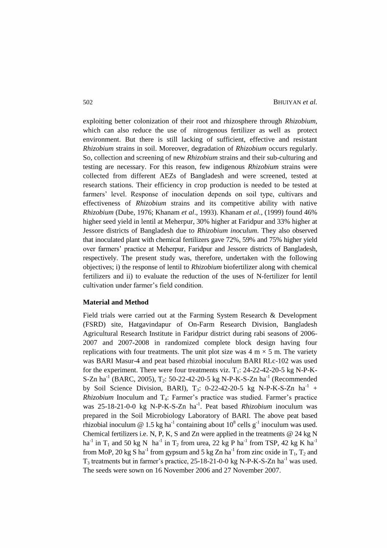
502 BHUIYAN et al.
exploiting better colonization of their root and rhizosphere through Rhizobium,
which can also reduce the use of nitrogenous fertilizer as well as protect
environment. But there is still lacking of sufficient, effective and resistant
Rhizobium strains in soil. Moreover, degradation of Rhizobium occurs regularly.
So, collection and screening of new Rhizobium strains and their sub-culturing and
testing are necessary. For this reason, few indigenous Rhizobium strains were
collected from different AEZs of Bangladesh and were screened, tested at
research stations. Their efficiency in crop production is needed to be tested at
farmers’ level. Response of inoculation depends on soil type, cultivars and
effectiveness of Rhizobium strains and its competitive ability with native
Rhizobium (Dube, 1976; Khanam et al., 1993). Khanam et al., (1999) found 46%
higher seed yield in lentil at Meherpur, 30% higher at Faridpur and 33% higher at
Jessore districts of Bangladesh due to Rhizobium inoculum. They also observed
that inoculated plant with chemical fertilizers gave 72%, 59% and 75% higher yield
over farmers’ practice at Meherpur, Faridpur and Jessore districts of Bangladesh,
respectively. The present study was, therefore, undertaken with the following
objectives; i) the response of lentil to Rhizobium biofertilizer along with chemical
fertilizers and ii) to evaluate the reduction of the uses of N-fertilizer for lentil
cultivation under farmer’s field condition.
Material and Method
Field trials were carried out at the Farming System Research & Development
(FSRD) site, Hatgavindapur of On-Farm Research Division, Bangladesh
Agricultural Research Institute in Faridpur district during rabi seasons of 2006-
2007 and 2007-2008 in randomized complete block design having four
replications with four treatments. The unit plot size was 4 m × 5 m. The variety
was BARI Masur-4 and peat based rhizobial inoculum BARI RLc-102 was used
for the experiment. There were four treatments viz. T1: 24-22-42-20-5 kg N-P-K-
S-Zn ha-1
(BARC, 2005), T2: 50-22-42-20-5 kg N-P-K-S-Zn ha-1
(Recommended
by Soil Science Division, BARI), T3: 0-22-42-20-5 kg N-P-K-S-Zn ha-1
+
Rhizobium Inoculum and T4: Farmer’s practice was studied. Farmer’s practice
was 25-18-21-0-0 kg N-P-K-S-Zn ha-1
. Peat based Rhizobium inoculum was
prepared in the Soil Microbiology Laboratory of BARI. The above peat based
rhizobial inoculum @ 1.5 kg ha-1 containing about 10
8 cells g
-1 inoculum was used.
Chemical fertilizers i.e. N, P, K, S and Zn were applied in the treatments @ 24 kg N
ha-1 in T1 and 50 kg N ha
-1 in T2 from urea, 22 kg P ha
-1 from TSP, 42 kg K ha
-1
from MoP, 20 kg S ha-1
from gypsum and 5 kg Zn ha-1 from zinc oxide in T1, T2 and
T3 treatments but in farmer’s practice, 25-18-21-0-0 kg N-P-K-S-Zn ha-1
was used.
The seeds were sown on 16 November 2006 and 27 November 2007.
RESPONSE OF LENTIL TO BIO AND CHEMICAL FERTILIZERS 503
Ta
ble
1.
Eff
ect
of
rhiz
ob
ial
ino
culu
m a
nd
ch
em
ica
l fe
rti
lize
rs o
n n
od
ula
tio
n,
dry
ma
tter
pro
du
ctio
n a
nd
yie
ld o
f le
nti
l a
t F
ari
dp
ur,
Ba
ng
lad
esh
(p
oo
led
da
ta o
f 2
yea
rs).
Tre
atm
ent
No
dule
nu
mb
er
pla
nt-1
No
dule
wei
ght
(mg p
lant-1
)
Ro
ot
wei
ght
(g p
lant-1
)
Sho
ot
wei
ght
(g p
lant-1
)
Pla
nt
hei
ght
(cm
)
Sto
ver
yie
ld
(t h
a-1)
10
00
seed
wei
ght
(g)
See
d
yie
ld
(t h
a-1)
Yie
ld
incr
ease
over
FP
(%)
T1:
N2
4P
22K
42S
20Z
n5
T2:
N5
0P
22K
42S
20Z
n5
T3:N
OP
22K
42S
20Z
n5+
Ino
c.
T4:F
P (
N2
0P
12K
17S
0Z
n0)
7.2
0b
6.1
6b
11
.62
a
6.8
5b
6.7
0b
6.4
5b
11
.94
a
6.6
7b
0.0
9
0.1
1
0.1
1
0.0
9
1.2
5
1.4
1
1.4
4
1.2
9
32
.4
34
.1
31
.6
32
.4
1.5
7
1.5
9
1.6
0
1.5
3
17
.4
17
.2
17
.4
17
.0
1.4
0a
1.3
4a
1.4
4a
0.9
9b
41
.4
35
.4
45
.5
-
CV
(%
) 1
5.5
1
4.5
1
3.6
1
2.0
6
.8
11
.4
4.7
9
.3
-
Mea
ns
foll
ow
ed b
y c
om
mo
n l
ette
r ar
e no
t si
gnif
ican
tly d
iffe
rent
at 5
% l
evel
by D
MR
T
T1:
N2
4P
22K
42S
20Z
n5
kg h
a-1,
T2:
N5
0P
22K
42S
20Z
n5 k
g h
a-1,
T3:
N0P
22K
42S
20Z
n5 k
g h
a-1 +
Rhiz
obiu
m i
no
culu
m,
T4:
FP
(N
20P
12K
17S
0Z
n0
kg h
a-1),
FP
= F
arm
er’s
pra
ctic
e
504 BHUIYAN et al.
During the experiment, growth and development of plants in the field were carefully observed. Ten plants along with roots were collected at 50% flowering
stage from each unit plot. The dry weight of roots; shoots and nodules including nodule numbers were recorded. The plants were harvested on 07 March for 2007 and 02 March for 2008. Data on plant height, 1000-seed weight, stover yield and seed yield were taken. All data were analyzed statistically.
Results and Discussion
Effect of Rhizobium inoculation and the application of chemical fertilizers on
nodule number (plant-1
), nodule weight (mg plant-1
), root weight (g plant-1
), shoot weight (g plant
-1), plant height (cm), 1000-seed weight (g), stover yield (t ha
-1),
seed yield (t ha-1
) and percent yield increased over farmer’s practice have been presented in Table 1.
The highest nodule number (11.62 plant-1
) and nodule weight (11.94 mg plant-1
) were recorded in PKSZn + Inoculum treated plot which was significantly higher
over other treatments (Table 1). The treatments T1, T2 and T4 produced identical nodule number and weight. Among the 4 treatments, T2 treatments (N24P22K42S20Zn5) produced the lowest nodule number and weight. Khanam et al., (1993) reported higher nodule number (156-245%) and nodule weight (169-284%) due to Rhizobium inoculation in lentil. Khanam et al., (1999) observed that Rhizobium inoculum gave 167%, 60% and 136% higher nodule mass over
control at Kustia, Faridpur and Jessore, respectively while Rhizobium inoculum plus chemical fertilizers except N gave 342%, 106% and 264% higher nodule mass at Meherpur, Faridpur and Jessore, respectively. Bhuiyan et al., (1996) also found higher nodule number (101%) at farmer’s field of Faridpur, Bangladesh and 110% at farmer’s field of Jessore, Bangladesh, and nodule weight 52% higher at Faridpur and 81% higher at farmer’s field at Jessore due to Rhizobim
inoculation in chickpea. Similar trends were also reported by Bhuiyan et al., (2001) for chickpea at farmers’ field of Meherpur and Rajshahi districts of Bangladesh. Root weight, shoot weight, plant height, stover yield and 1000-seed weight were found insignificant, though the highest values were observed in PKSZn + Inoculum treatment. Similar results were reported by Bhuiyan et al., (2001) in chickpea at Rajshahi, Bangladesh. The seed yield was significantly
influenced by inoculum. The highest seed yield 1.44 t ha-1
were recorded with the treatment P22K42S20Zn5 + Inoculum but identical with T1 and T2 treatments. The seed yield showed higher 1.44 t ha
-1 due to higher pods plant
-1, seeds pod
-1 and
1000-seed weight. The similar trend was also reported by Khanam et al., (1993). They reported that Rhizobium inoculation gave 64-68% higher seed yield in lentil. In another study, Khanam et al., (1999) found 46% higher seed yield in
lentil at Meherpur, 30% at Faridpur and 33% at Jessore districts of Bangladesh due to Rhizobium inoculum. The lower seed yield was recorded in T2 treatment than T1 which might be due to excess plant growth and less pod setting. The lowest yield was with farmer’s practice (0.99 t ha
-1). Rhizobium inoculum with

RESPONSE OF LENTIL TO BIO AND CHEMICAL FERTILIZERS 505
inorganic fertilizer T3, showed better performance against only with inorganic fertilizers T1 and T2 treatments. The yield was 100 kg higher than T2 due to
application of Rhizobium inoculum. So, Rhizobium inoculum can be used as the substitute of urea for lentil cultivation at Faridpur area. Khanam et al., (1999) also observed that inoculated plant with chemical fertilizers gave 72%, 59% and 75% higher yield over farmers’ practice at Meherpur, Faridpur and Jessore districts of Bangladesh, respectively. The results are also an agreement with the findings of Bhuiyan et al., (1998).
Farmers’ reaction
The farmer’s of Faridpur district were very encouraged by observing the
performance of BARI Masur-4 with rhizobial inoculum.
Economic analysis
Benefit cost ratio (BCR) analysis for lentil at Faridpur has been presented in
Table 2. For BCR only cost of chemical fertilizers and Rhizobium inoculum were
considered and other costs remain constant. Economic analysis revealed that T3
treatment i.e. PKSZn with inoculum gave the highest BCR 5.36 at Faridpur.
Khanam et al., (1993) found that inoculated treatment with PKSZn fertilizers
gave higher benefit cost ratio 6.44-7.68 in lentil. Bhuiyan and Khanam (1996)
found BCR 8.71-9.61 by PKSZn + Rhizobium inoculum in chickpea.
Table 2. Benefit cost ratio analysis for lentil at Faridpur (mean of 2 years).
Treatments
Yield
(t ha-1
)
Variable
cost
(Tk. ha-1
)
Gross
return
(Tk. ha-1
)
Net
return
(Tk. ha-1
)
Net return
over
farmer’s
practice (Tk.
ha-1
)
Benefit
cost
ratio
T1: N24P22K42S20Zn5 1.40 5,948/- 1,05,000/- 99,052/- 27,848/- 4.68
T2: N50P22K42S20Zn5 1.34 6,348/- 1,00,500/- 94,152/- 22,948/- 3.61
T3:N0P22K42S10Zn5+Inoc. 1.44 5,728/- 1,07,625/- 1,01,897/- 30,693/- 5.36
T4: FP(N25P18K21S0Zno) 0.99 2,671/- 73,875/- 71,204/- - -
Urea= Tk. 7.00 kg-1
, TSP= Tk. 17.00 kg-1
, MoP= Tk. 18.00 kg-1
, Gypsum= Tk. 8.00 kg-1
,
ZnSO4= Tk. 95.00 kg-1
, Rhizobium inoculum = Tk. 100 kg-1
, Lentil= Tk. 75.00 kg-1
For both the years, positive and significant correlation was found in nodule number
with nodule weight (Table 3). Nodule number was strongly correlated with nodule
weight. Nodule number was also correlated with root weight in 2007 and nodule
weight was correlated with shoot weight and stover yield in 2008 (Table 3).
Bhuiyan et al., (1996 and 2001) also reported positive and significant correlation for
the inoculated chickpea.
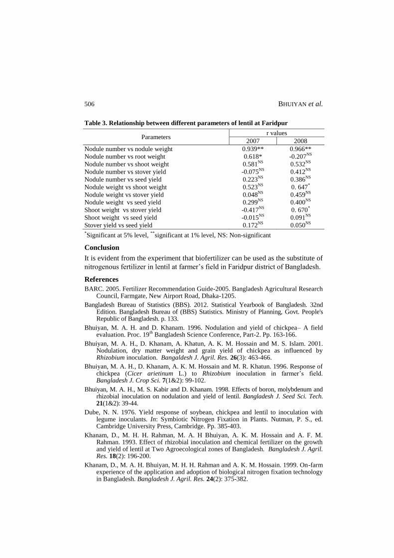
506 BHUIYAN et al.
Table 3. Relationship between different parameters of lentil at Faridpur
Parameters r values
2007 2008
Nodule number vs nodule weight 0.939** 0.966**
Nodule number vs root weight 0.618* -0.207NS
Nodule number vs shoot weight 0.581NS
0.532NS
Nodule number vs stover yield -0.075NS
0.412NS
Nodule number vs seed yield 0.223NS
0.386NS
Nodule weight vs shoot weight 0.523NS
0. 647*
Nodule weight vs stover yield 0.048NS
0.459NS
Nodule weight vs seed yield 0.299NS
0.400NS
Shoot weight vs stover yield -0.417NS
0. 670*
Shoot weight vs seed yield -0.015NS
0.091NS
Stover yield vs seed yield 0.172NS
0.050NS
*Significant at 5% level,
**significant at 1% level, NS: Non-significant
Conclusion
It is evident from the experiment that biofertilizer can be used as the substitute of
nitrogenous fertilizer in lentil at farmer’s field in Faridpur district of Bangladesh.
References
BARC. 2005. Fertilizer Recommendation Guide-2005. Bangladesh Agricultural Research Council, Farmgate, New Airport Road, Dhaka-1205.
Bangladesh Bureau of Statistics (BBS). 2012. Statistical Yearbook of Bangladesh. 32nd Edition. Bangladesh Bureau of (BBS) Statistics. Ministry of Planning, Govt. People's Republic of Bangladesh. p. 133.
Bhuiyan, M. A. H. and D. Khanam. 1996. Nodulation and yield of chickpea– A field evaluation. Proc. 19
th Bangladesh Science Conference, Part-2. Pp. 163-166.
Bhuiyan, M. A. H., D. Khanam, A. Khatun, A. K. M. Hossain and M. S. Islam. 2001. Nodulation, dry matter weight and grain yield of chickpea as influenced by Rhizobium inoculation. Bangaldesh J. Agril. Res. 26(3): 463-466.
Bhuiyan, M. A. H., D. Khanam, A. K. M. Hossain and M. R. Khatun. 1996. Response of chickpea (Cicer arietinum L.) to Rhizobium inoculation in farmer’s field. Bangladesh J. Crop Sci. 7(1&2): 99-102.
Bhuiyan, M. A. H., M. S. Kabir and D. Khanam. 1998. Effects of boron, molybdenum and rhizobial inoculation on nodulation and yield of lentil. Bangladesh J. Seed Sci. Tech. 21(1&2): 39-44.
Dube, N. N. 1976. Yield response of soybean, chickpea and lentil to inoculation with legume inoculants. In: Symbiotic Nitrogen Fixation in Plants. Nutman, P. S., ed. Cambridge University Press, Cambridge. Pp. 385-403.
Khanam, D., M. H. H. Rahman, M. A. H Bhuiyan, A. K. M. Hossain and A. F. M. Rahman. 1993. Effect of rhizobial inoculation and chemical fertilizer on the growth and yield of lentil at Two Agroecological zones of Bangladesh. Bangladesh J. Agril. Res. 18(2): 196-200.
Khanam, D., M. A. H. Bhuiyan, M. H. H. Rahman and A. K. M. Hossain. 1999. On-farm experience of the application and adoption of biological nitrogen fixation technology in Bangladesh. Bangladesh J. Agril. Res. 24(2): 375-382.

ISSN 0258-7122
Bangladesh J. Agril. Res. 40(3): 507-512, September 2015 Short Communication
INCIDENCE, DAMAGE POTENTIAL AND MANAGEMENT OF
JASSIDS IN GROUNDNUT FIELD
DR. G. C. BISWAS1
Keywords : Incidence, damage severity, jassid, groundnut.
The studies were made on the incidence, damage severity and management of
jassid in groundnut in the experimental field during Rabi season of two
consecutive years 2011-12 and 2012-13. The highest jassid population
(24.25/plant) and leaf infestation (54.25%) were observed in the second week of
April at the pod formation stage of the crop. Among the treatments,
Imidaclorprid (Admire 200Sl @ 0.50ml/l) reduced significantly the highest jassid
population (80.25%) as well as leaf infestation (54.25%) over the untreated
control. The pod yield was significantly highest (1.60 t/ha) obtained from Admire
treated plot and calculated high BCR (3.16) followed by Dimethoid (Tafgor
40EC @ 2ml/l) treated plot having pod yield of 1.53t/ha and BCR 2.60.
Groundnut (Arachis hypogaea L.) is the second important oilseed crop after
rapeseed and mustard on the basis of area and annual production in Bangladesh
(Biswas et al., 2000). Its cultivation covered about 95,000 hectares of land and
produced about 1,40,000 metric tones of seeds during 2011-2012 (Anon. 2013).
It is a good source of oil (48-52%) and protein (25-30%) (Kaul and Das 1986).
Jassid ( Empoasca terminalis) the important foliage pest of groundnut and acts as
limiting factors in successful cultivation of the crop in South- East Asia
especially in India and Bangladesh (Ahmed et al., 1989; Begum, 1995; Biswas
et al., 2000; Biswas et al., 2009 ; Biswas and Das 2011; and Singh, 1990). Both
the nymphs and adults of Jssids suck the sap from the tender leaf and under
surface of the leaflet causing yellowing the leaflets, leaf curling, necrosis. V
shaped yellowing appears at the tip of the leaflets resulting stunted growth and
gradually die. It also acts as a vector of leaf curled, tomato spotted and other
viruses (Singh, 1990). Infested leaves become spotted, pale and sickly curled
(Amin and Palmer, 1985). Incidence of jassid on groundnut crop, losses, and
suitable management techniques are of very important. Information on these
aspects of jassid in groundnut crop field are scanty in Bangladesh. The research
work was undertaken to know the incidence, extent of damage and to develop the
suitable management techniques for jassid in groundnut crop.
The experiment was conducted in the field of the Oilseed Research Centre,
Bangladesh Agricultural Research Institute (BARI), Joydebpur, Gazipur, during
Rabi season of two consecutive years 2011-12 and 2012-13. Seeds of groundnut
variety BARI Chinabadam-9 were sown on November 27, 2011 and 2012 in 4m
1Principal Scientific Officer, Vertebrate Pest Division, Bangladesh Agricultural Research
Institute (BARI), Joydebpur, Gazipur-1701, Bangladesh

508 BISWAS
X 3m plots in Randomized Complete Block design with 3 replications. There
were five treatments, namely, application of detergent (Jet powder) 3g/litre,
Crude Neem seed mixture (NSM) @ 50 g/l, Spraying of Dimethoid (Tafgor 40
EC @ 2ml/l), Spraying of Imidaclorprid (Admire 200Sl) @ 0.5 ml/l of water and
Untreated control with only water were used uniformly. The recommended
agronomic practices like fertilizers and other intercultural operations were
maintained for raising the crop (Mondal and Wahhab, 2001).
Fresh ripe and sun dried neem seeds (5 kg) were crushed and then added 10 litres
of water and kept over night. Then the solution was sieved with fine mesh net
and added 10 g of detergent and the solution was prepared for spray. This is
known as crude neem seed and detergent mixture. The detergent, botanicals and
other insecticides were applied with the help of knapsack sprayer in three
frequencies on the crop in second and last week of February 2012 and 2013 at the
vegetative and flowering stages of the crop at 10 days intervals. The population
of jassids were recorded from the crop during February - May in both the years.
The leaf infestation caused by jassids was recorded on February - May in 2012
and 2013 at the vegetative, flowering and pod forming stages of the crop.
Randomly 10 plants were selected per plot for counting jassid population.
Percent leaf damage by jassids was recorded by counting leaves from five (5)
selected plant population in each treatment. Percent leaf infestation reduction
over untreated in each treatment was calculated. The crop was harvested on last
week of May in each year. Seed yield of different treatments were recorded.
Weather data mainly temperature was also recorded during the study period in
both the years. Data were compiled and analyzed statistically. Analysis of
variance (ANOVA) was done following MSTATE C and means were separated
following Duncan’s multiple range test (DMRT). Benefit cost ratio (BCR) of the
different treatments was also calculated.
Jassid population was observed in the groundnut crop during first week of
February in 2012 at the vegetative and flowering stages of the crop and continued
up to second week of May at the pod formation stage. The maximum jassid
population was observed (24.25/plant) in the second week of April 2012 and then
gradually decreased (Fig.1). Almost similar increasing trend of jassid population
was observed during 2013. But slightly higher jassid population (25.68/plant)
was observed in 2013 than in 2012 (Fig. 2). Leaf infestation by jassid showed the
similar pattern in both the years. The highest leaf infestation caused by jassid was
52.54% recorded in 2012 (Fig. 1) and slightly higher leaf infestation rate by
jassid (55.68/plant) in 2013 than in 2012 (Fig. 2). It was observed that jassid
population and leaf infestation in groundnut crop increased in time with the
increasing average temperature (From 230 C -30
0 C ) in two years (Figs 1 and 2.).
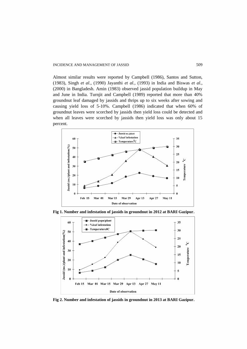
INCIDENCE AND MANAGEMENT OF JASSID 509
Almost similar results were reported by Campbell (1986), Santos and Sutton,
(1983), Singh et al., (1990) Jayanthi et al., (1993) in India and Biswas et al.,
(2000) in Bangladesh. Amin (1983) observed jassid population buildup in May
and June in India. Turnjit and Campbell (1989) reported that more than 40%
groundnut leaf damaged by jassids and thrips up to six weeks after sowing and
causing yield loss of 5-10%. Campbell (1986) indicated that when 60% of
groundnut leaves were scorched by jassids then yield loss could be detected and
when all leaves were scorched by jassids then yield loss was only about 15
percent.
Fig 1. Number and infestation of jassids in groundnut in 2012 at BARI Gazipur.
Fig 2. Number and infestation of jassids in groundnut in 2013 at BARI Gazipur.

510 BISWAS
Efficacy of jet powder, neem seed mixture and chemical insecticides in controlling jassids in groundnut crop during 2012 and 2013 is presented in
Table 1. All the treatments reduced jassid population with significant variation among them. Of these Imidaclorprid (Admire 200SL @ 0.50ml/l) reduced significantly the highest jassid population (80.25%) over the untreated. Reduction of jassid occurred by 65-68% in Tafgor (Dimethoid) 40 EC @2ml/l and neem seed mixture+Jet powder treated plots and these two treatments caused similar controlling effects on jassid next to Imidaclorprid (admire,
82.72%) while Jet powder @ 3g/l reduced the lowest jassid population (49.86%) over the untreated control. The leaf infestation by jassid had the same trend as the number in all the treatments with the highest efficacy of Imidaclorprid resulted 80.72% reduction over untreated control. The lowest efficacy was recorded in jet powder treatment (Table 2). Almost similar information was recorded by Campbell (1986) in India and Biswas et al., (2009
and 2011) in Bangladesh.
Table 1. Number of jassids and reduction of its population over control in different
treatments in groundnut crop in two years pooled data.
Treatments
Number of jassid/plant after three times of
spray % Population
reduction
over untreated 7 days after
1st spray
7 days after
2nd spray
7 days after
3rd spray Mean
Jet powder @ 3g/L 15.60 b 10.40 b 08.00 b 11.40 b 49.86 c
NSM + jet powder 12.00 c 08.50 c 06.50 c 8.80 c 65.07 b
Tafgor @ 2 ml/L 10.00 c 06.50 c 05.50 c 7.66 c 68.58 b
Admire @0.5 ml/L 08.50 d 05.50 d 02.00 d 5.00 d 80.72 a
Untreated 20.50 a 25.50 a 35.00 a 25.67 a -
Means followed by the same letter in a column did not differ significantly at 5% level by
DMRT. Neem Seed Mixture= NSM.
Table 2. Percent of leaf infestation in different treatments used against jassids in
groundnut in the pooled data of 2012 and 2013 at Gazipur.
Treatments
Leaf infestation(%) by jassid recorded on % infestation
reduction
over
untreated
7 days
after 1st
spray
7 days after
2nd spray
7 days
after
3rd spray
Mean leaf
infestation
(%)
Jet powder @ 3g/L 30.60 b 21.40 b 18.00 b 23.40 b 49.86 c
NSM + jet powder 23.00 c 15.50 c 10.50 c 16.30 c 65.07 b
Tafgor @ 2 ml/L 22.00 c 13.50 c 8.50 c 14.66 c 68.58 b
Admire @0.5 ml/L 13.50 d 8.50 d 5.00 d 9.00 d 80.72 a
Untreated 40.50 a 56.50 a 65.00 a 54.67 a -
Means followed by the same letter in a column do not differ significantly at 5% level by
DMRT. Data were recorded in average of 10 plants/plot. . Neem Seed Mixture= NSM.

INCIDENCE AND MANAGEMENT OF JASSID 511
Table 3. Benefit cost ratio of different treatments against jassid in groundnut from
the pooled data of 2012 and 2013 at BARI, farm Gazipur
Treatments
Seed
yield
(t/ha)
Increased
yield over
untreated
Addition
al
income
(TK./ha)
Cost of
insectici
des
& spray
Net
income
(TK./ha)
BCR
Jet powder @3g/L 1.43 bc 0.08 4000.00 1500.00 2500.00 1.66
NSM + jet powder 1.48 ab 0.13 6500.00 2000.00 4500.00 2.25
Tafgor @ 2ml/L 1.53 ab 0.18 9000.00 2500.00 6500.00 2.60
Admire @0.5 ml/L 1.60 a 0.25 12500.00 3000.00 9500.00 3.16
Untreated 1.35 d - - -
Means followed by the same letters in a column do not differ significantly at 5% level by
DMRT.
Price of Jet powder = 250, Price of Admire = 10000 Tk./L, Price of Tafhor = 800 TK./L
Price of groundnut seed= 50 Tk./kg, Cost of neem seed = 50 Tk./Kg, Cost of labour=200
Tk./labour/day , Three labours and 0.5 litre of Tafgor 40 EC @ 2 ml/I being required for
1 hectare of crop field sprayed in one time. One machine spray volume = 10 litre
required 200 sqm field spraying in one time. Other variable costs were same in all the
treatments.
BCR= Net income/ Management cost
The Benefit Cost Ratio (BCR) analysis of different treatments in suppressing
jassids in groundnut crop is presented in the Table 3. The result revealed that
significantly the highest pod yield of groundnut was obtained from Admire 200
Sl treated plot (1.60 t/ha) and calculated the highest BCR (3.16) followed by that
of Tafgor 40 EC treated plot (2.60). The groundnut pod yield was 1.53 t/ha which
was not statistically significant different from that of neem seed mixture + jet
powder treated plot (Table 3). Significantly the lowest pod yield was recorded
from the untreated control plot (1.35t/ha) and the lowest BCR was calculated
from Jet powder treated plot (1.66)(Table 3). Similar information was also
reported by Amin and palmer (1985), Singh (1990) in India and Ahmed et al.,
(1989) and Biswas et al., (2009 and 2011) in Bangladesh.
References
Anonymous, 2013. Krishi Diary-2013, Crop production target and achieved 2011-12.
Agricultural Information Service, Department of Agricultural Extension,
Khamarbari, Dhaka-1215, pp.98.
Ahmed, K. N., M. M. Husain and U. Islam. 1989. A preliminary report on the insect pests
of groundnut. J. Asiat. Soc. Bangladesh Sci. 15: 31 – 35.
Amin, P.W. 1983. Major field insect pests of groundnut in India and associated crop
losses. Indian J. Entom. (Special issue) 2: 337-344.

512 BISWAS
Amin, P.W. and J. Palmer. 1985. Identification of groundnut Thysanoptera. Tropical Pest
Management 31: 286-291.
Begum, S. 1995. Insect pests of oilseed crops of Bangladesh. Bangladesh J. Zool. 23(2):
153-158.
Biswas, G.C., F. U. Mian and M.S. Islam 2000. Screening of some groundnut genotypes
for resistance to jassids infestation. Bangladesh J. Agril Res. 25 (2): 721-725.
Biswas, G.C., S. Begum, and M.Y. Mian. 2000. Leaf infestation and yield loss caused by
jassid and thrips in groundnut. J. Asiat. Soc. Bangladesh Sci. 26 (2): 253-258.
Biswas, G.C., K.H. Kabir and R. Islam 2009. Insect pest management of oilseed crops in
Bangladesh.pp.109-122. In: Advances in oilseed research in Bangladesh edited by
Bakr and Ahmed. Proceedings of the National Workshop Prospects and
Development of Oilseed crops in Bangladesh and Future Challenges 29-30 April
2009.
Biswas, G. C. and G. P. Das. 2011. Insect and mite pests diversity in the oilseed crops
ecosystems in Bangladesh. Bangladesh J. Zool. 39 (2): 232-235.
Campbell, W.V. 1986. Management of arthropods on peanut in South-east asia. In
University of Georgia, Annual report, Peanut Collaborative Research Support
Program, 115-133.
Jayanthi, M., K. M. Singh and R. N. Singh. 1993. Succession of insect pest on high
yielding groundnut variety under Delhi conditions. Indian J. Ent. 55 (7): 24-29.
Kaul, A. K. and M. L Das 1986. “Oilseeds in Bangladesh.” Bangladesh Canada
Agriculture Sector Team. Ministry of Agriculture, Govt. of the People’s Republic of
Bangladesh, Dhaka. 324 p.
Mondal, M.R.I. and M.A. Wahhab 2001. “Production Technology of Oilcrops.” Oilseed
Research Centre, BARI, Joydebpur, Gazipur. 111 p.
Santos, R.B. and B.G. Sotton.1983. effect of Defoliation on reproductive development of
the peanut. Austalian J. Agric. Research, 34: 527-535.
Singh, S.R. 1990. Insect Pest of Tropical Food Legumes. John Willy & Sons.Inc. New
York, USA. pp. 451.
Singh, T.V. K., K.M. Singh and R.N. Singh 1990. Groundnut Pest complex, succession
of pests. Indian J. Ent. 52 (3): 493-498.
Turnjit J.A. and W. V. Campbell 1989. Peanut communication about groundnut pests.
Tropical Grain Legume Bull. 26: 23-25.
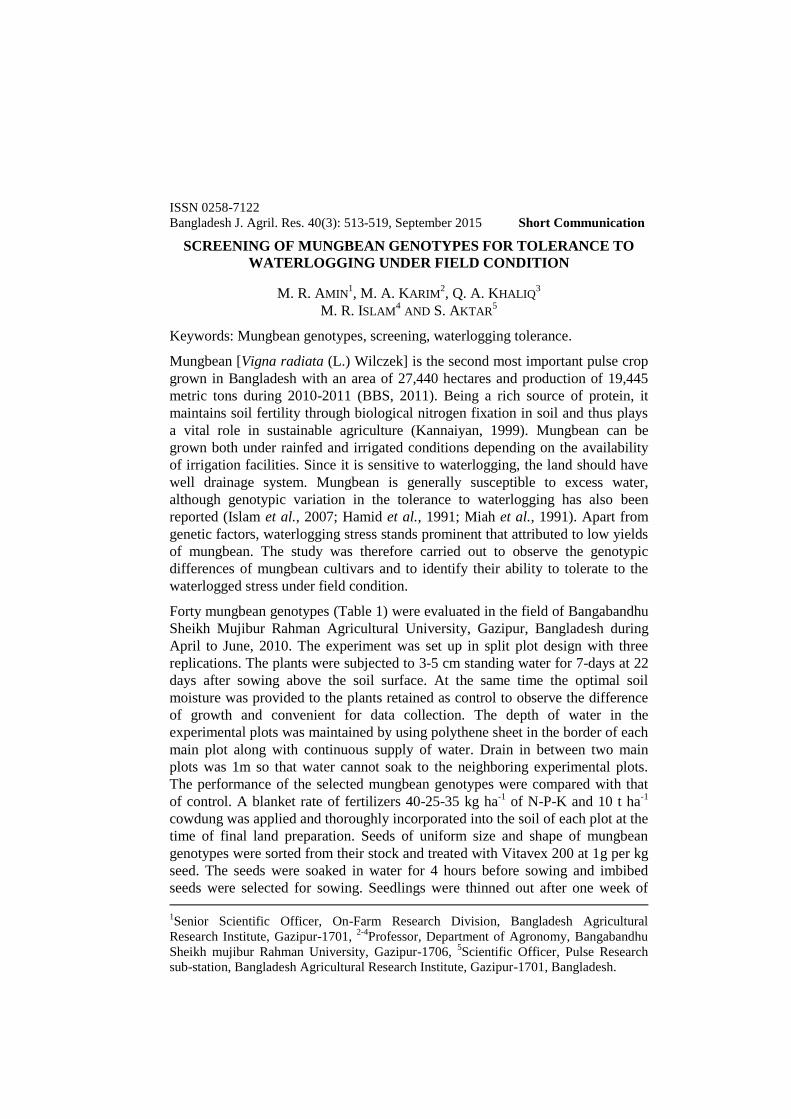
ISSN 0258-7122
Bangladesh J. Agril. Res. 40(3): 513-519, September 2015 Short Communication
SCREENING OF MUNGBEAN GENOTYPES FOR TOLERANCE TO
WATERLOGGING UNDER FIELD CONDITION
M. R. AMIN1, M. A. KARIM
2, Q. A. KHALIQ
3
M. R. ISLAM4 AND S. AKTAR
5
Keywords: Mungbean genotypes, screening, waterlogging tolerance.
Mungbean [Vigna radiata (L.) Wilczek] is the second most important pulse crop
grown in Bangladesh with an area of 27,440 hectares and production of 19,445
metric tons during 2010-2011 (BBS, 2011). Being a rich source of protein, it
maintains soil fertility through biological nitrogen fixation in soil and thus plays
a vital role in sustainable agriculture (Kannaiyan, 1999). Mungbean can be
grown both under rainfed and irrigated conditions depending on the availability
of irrigation facilities. Since it is sensitive to waterlogging, the land should have
well drainage system. Mungbean is generally susceptible to excess water,
although genotypic variation in the tolerance to waterlogging has also been
reported (Islam et al., 2007; Hamid et al., 1991; Miah et al., 1991). Apart from
genetic factors, waterlogging stress stands prominent that attributed to low yields
of mungbean. The study was therefore carried out to observe the genotypic
differences of mungbean cultivars and to identify their ability to tolerate to the
waterlogged stress under field condition.
Forty mungbean genotypes (Table 1) were evaluated in the field of Bangabandhu
Sheikh Mujibur Rahman Agricultural University, Gazipur, Bangladesh during
April to June, 2010. The experiment was set up in split plot design with three
replications. The plants were subjected to 3-5 cm standing water for 7-days at 22
days after sowing above the soil surface. At the same time the optimal soil
moisture was provided to the plants retained as control to observe the difference
of growth and convenient for data collection. The depth of water in the
experimental plots was maintained by using polythene sheet in the border of each
main plot along with continuous supply of water. Drain in between two main
plots was 1m so that water cannot soak to the neighboring experimental plots.
The performance of the selected mungbean genotypes were compared with that
of control. A blanket rate of fertilizers 40-25-35 kg ha-1
of N-P-K and 10 t ha-1
cowdung was applied and thoroughly incorporated into the soil of each plot at the
time of final land preparation. Seeds of uniform size and shape of mungbean
genotypes were sorted from their stock and treated with Vitavex 200 at 1g per kg
seed. The seeds were soaked in water for 4 hours before sowing and imbibed
seeds were selected for sowing. Seedlings were thinned out after one week of
1Senior Scientific Officer, On-Farm Research Division, Bangladesh Agricultural
Research Institute, Gazipur-1701, 2-4
Professor, Department of Agronomy, Bangabandhu
Sheikh mujibur Rahman University, Gazipur-1706, 5Scientific Officer, Pulse Research
sub-station, Bangladesh Agricultural Research Institute, Gazipur-1701, Bangladesh.
514 AMIN et al.
emergence keeping one healthy seedlings per hill. Management practices and
plant protection measures were taken as and when necessary. Five plants both
from control and waterlogging treatments were harvested after 28 and 38 days
from their corresponding emergence dates and data were collected. Height of
individual plants was measured from the base to the top of main shoot. After
harvesting, the seedlings of both waterlogged and controls were segmented into
components i.e. stem, leaf, petiole, and reproductive organs. The segmented parts
were oven dried at 800C for 72 hours to a constant weight and dry weights were
recorded separately. Total dry weight was calculated by summing up the dry
weights of stem, leaf, petiole, and reproductive parts of plants. Leaf area was
measured using automatic leaf area meter (Model AAM-8. Hayashi Denkoh Co.
Ltd., Tokyo, Japan). The screening criterion of the genotypes was based on
survival % after removal of the flooding stress. Their survival percentage was
recorded on the 28 DAE, 38 DAE and 48 DAE after termination of flooding.
Plant survival percentage of each genotype was calculated by the following
formula,
The no. of plants of each genotype survived after 7-day waterlogging
Survival (%) = ---------------------------------------------------------------------------x100 Total plants of each genotype present at the beginning of waterlogging
The screening criterion of the genotypes was based on survival rate and recovery
of plants after termination of waterlogging as suggested by Nawata (1989). After
termination of waterlogging (28 DAE), a significant number of plants of each
genotypes were found to survive. During 10-days recovery period (38 DAE), the
number of plants of each genotype greatly reduced due to seedling mortality.
Finally, a number of plants of each mungbean genotype were survived till
maturity. The percentage of plant survival was calculated (Table 1). Among the
total number of genotypes, only 15 genotypes namely, IPSA-13 (entry no.26),
IPSA-15 (entry no.27), VC-3173 (B-10) (entry no.28), VC-6367 (44-55-2) (entry
no.29), ACC-12890054 (entry no.30), ACC-12890085 (entry no.31), GK-1(entry
no.32), GK-3 (entry no.33), GK-63 (entry no.34), GK-48 (entry no.35), GK-65
(entry no.36), BU mug 2 (entry no.37), CO-3 (entry no.38), VC-6173A (entry
no.39), VC-3160(A-89) (entry no.40) showed 20-34% survival, and the rest 25
genotypes had survival of <20%. Lawn and Russel (1978) reported that after
emergence, the stand establishment of the mungbean crop may reduce to 65-
100% for eight days waterlogging at second trifoliate leaf stage.
The variability in plant characters of the mungbean genotypes at the end of
waterlogging (28 DAE) and during 10 days recovery period (38 DAE) have been
shown in Table 2. Some plants were taller viz. IPK-1040-94 (entry no.3), ML-
613 (entry no.5), GK-46 (entry no.11), PDM-11 (entry no.23), ACC-12890054
(entry no.30), ACC-12890085 (entry no.31), GK-63 (entry no.34), GK-48 (entry
no.35), CO-3 (entry no.38) and some were shorter viz. GK-29 (entry no.19), GK-

SCREENING OF MUNGBEAN GENOTYPES FOR TOLERANCE 515
55 (entry no.20), VC-6367 (44-55-2) (entry no.29), GK-1 (entry no.32), GK-48
(entry no.35) under control condition but significant reduction in plant height of
all the waterlogged treated genotypes was observed. The difference in plant
height of waterlogged plants were increased to a great extent during 10 days
recovery period and less reduction in plant height over the control was recorded
35.59 % in BARI mung 6, 76 % in BARI mung 5, 29.33 %, in GK-6 and 3.85 %
in BU mug 2. The relative elongation rate of plant height is a morphological
mechanism of waterlogged tolerance of plants as reported by Futakuchi et al.,
(2001).
Table 1. List of mungbean genotypes and percentage of plant survived at 28, 38 and
48 days after emergence of seedlings
Sl.
no. Genotypes
% of plant survival
at 28 DAE
% of plant survival
at 38DAE
% of plant
survival
at 48DAE
1 BINA-6 65.21 13.04 4.34
2 BINA-7 66.66 17.77 6.66
3 IPK-1040-94 83.33 14.28 9.52
4 IPSA -18 63.15 21.05 7.89
5 ML-613 74.41 20.93 6.97
6 GK-6 55.88 11.76 2.94
7 GK-7 57.57 12.12 3.03
8 GK-32 55.88 17.64 8.82
9 GK-36 65.90 13.63 6.81
10 GK-37 63.88 13.88 8.33
11 GK-46 62.22 13.33 6.66
12 VC-3950-88 76.74 13.95 2.32
13 BARI mung 5 69.44 22.22 19.44
14 BARI mung 6 76.31 21.05 10.52
15 IPSA-12 35.00 25.00 17.50
16 IPSA-19 57.77 22.22 13.33
17 GK-5 58.33 16.66 11.11
18 GK14 58.13 16.27 13.95
19 GK-29 60.52 21.05 19.44
20 GK-55 61.53 20.51 15.38
21 GK-56 63.15 18.42 10.52
22 ML-267 71.42 23.80 16.66
23 PDM-11 75.00 18.18 11.36

516 AMIN et al.
Table 1. Continued.
Sl.
no. Genotypes
% of plant survival
at 28 DAE
% of plant survival
at 38DAE
% of plant
survival
at 48DAE
24 VC-6379 (23-11) 70.21 21.27 10.63
25 VC-3173 (B-6) 80.95 19.04 11.90
26 IPSA-13 76.92 23.07 20.51
27 IPSA-15 61.90 28.57 21.42
28 VC-3173 (B-10) 68.18 36.36 29.54
29 VC-6367(44-55-2) 77.77 31.11 26.66
30 ACC-12890054 66.66 28.57 23.80
31 ACC-12890085 73.33 28.88 22.22
32 GK-1 65.78 23.68 21.05
33 GK-3 66.66 25.64 25.64
34 GK-63 60.52 26.31 21.05
35 GK-48 66.66 27.27 24.24
36 GK-65 65.00 25.00 22.50
37 BU mug 2 81.81 43.18 34.09
38 CO-3 85.71 33.33 30.95
39 VC-6173 A 81.25 46.87 31.25
40 VC-3160 (A-89) 71.42 33.33 30.95
Leaf area (cm2
plant-1
) increased significantly in control plants over time and
decreased significantly in flooded plants at the end of waterlogging (28 DAE).
The reduction in leaf area over control ranged from 6% to 80% in different
genotypes among which comparatively higher recovery in leaf area was recorded
in (BINA-7) 27% (entry no.2), (IPSA-19) 38% (entry no.16), (GK-29) 26%
(entry no.29), (GK-56) 36% (entry no.21), {VC-6379 (23-11)} 6% (entry no.24),
{VC-3173 (B-10)} 1% (entry no.28), {VC-6367 (44-55-2)}29% (entry no.29),
(VC3950-88) 34% (entry no.12), (ACC-12890085) 11% (entry no.31). While
higher leaf area during the recovery period (28 DAE) indicated greater foliage
development ability of some mungbean genotypes overcoming waterlogging
stress reported by Islam (2005).
Plant components such as stem, leaf, and petiole and pod dry weight varied in
between the control and waterlogged plants. A wide range of genetic variation in
waterlogging induced changes in dry matter accumulation in the plant component
observed by Islam et al., (2007). The dry matter weight of plant parts in different
mungbean genotypes reduced greatly after waterlogging and increased
considerably during 10 days recovery period. Some genotypes produced pods
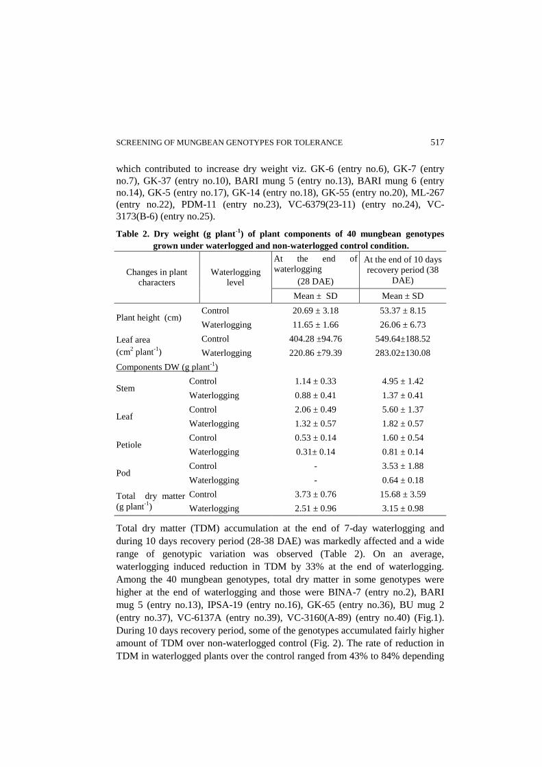
SCREENING OF MUNGBEAN GENOTYPES FOR TOLERANCE 517
which contributed to increase dry weight viz. GK-6 (entry no.6), GK-7 (entry
no.7), GK-37 (entry no.10), BARI mung 5 (entry no.13), BARI mung 6 (entry
no.14), GK-5 (entry no.17), GK-14 (entry no.18), GK-55 (entry no.20), ML-267
(entry no.22), PDM-11 (entry no.23), VC-6379(23-11) (entry no.24), VC-
3173(B-6) (entry no.25).
Table 2. Dry weight (g plant-1
) of plant components of 40 mungbean genotypes
grown under waterlogged and non-waterlogged control condition.
Changes in plant
characters
Waterlogging
level
At the end of
waterlogging
(28 DAE)
At the end of 10 days
recovery period (38
DAE)
Mean ± SD Mean ± SD
Plant height (cm) Control 20.69 ± 3.18 53.37 ± 8.15
Waterlogging 11.65 ± 1.66 26.06 ± 6.73
Leaf area
(cm2 plant
-1)
Control 404.28 ±94.76 549.64±188.52
Waterlogging 220.86 ±79.39 283.02±130.08
Components DW (g plant-1
)
Stem Control 1.14 ± 0.33 4.95 ± 1.42
Waterlogging 0.88 ± 0.41 1.37 ± 0.41
Leaf Control 2.06 ± 0.49 5.60 ± 1.37
Waterlogging 1.32 ± 0.57 1.82 ± 0.57
Petiole Control 0.53 ± 0.14 1.60 ± 0.54
Waterlogging 0.31± 0.14 0.81 ± 0.14
Pod Control - 3.53 ± 1.88
Waterlogging - 0.64 ± 0.18
Total dry matter
(g plant-1
)
Control 3.73 ± 0.76 15.68 ± 3.59
Waterlogging 2.51 ± 0.96 3.15 ± 0.98
Total dry matter (TDM) accumulation at the end of 7-day waterlogging and
during 10 days recovery period (28-38 DAE) was markedly affected and a wide
range of genotypic variation was observed (Table 2). On an average,
waterlogging induced reduction in TDM by 33% at the end of waterlogging.
Among the 40 mungbean genotypes, total dry matter in some genotypes were
higher at the end of waterlogging and those were BINA-7 (entry no.2), BARI
mug 5 (entry no.13), IPSA-19 (entry no.16), GK-65 (entry no.36), BU mug 2
(entry no.37), VC-6137A (entry no.39), VC-3160(A-89) (entry no.40) (Fig.1).
During 10 days recovery period, some of the genotypes accumulated fairly higher
amount of TDM over non-waterlogged control (Fig. 2). The rate of reduction in
TDM in waterlogged plants over the control ranged from 43% to 84% depending

518 AMIN et al.
on the genotypes. Lower reduction in TDM over the control was recorded in
BARI mung 5 (65%), IPSA-12 (61%), IPSA-13 (61%), IPSA-15 (47%), VC-
3173(B-10) (65%), VC-6367(44-55-2) (51%), ACC-12890054 (51%), ACC-
128900850 (43%), VC-6173A (61%). Accumulation of higher TDM in
waterlogged plants over the control was observed in some mungbean genotypes
which might tolerate soil flooding to a great extent. Yadav and Saxena (1998)
found decreased production of total dry matter in waterlogged mungbean.
Fig.1. Total dry matter of mungbean genotypes at the end of 7-day waterlogging
Fig. 2. Total dry matter of mungbean genotypes at the end of 10 days recovery
period
0
1
2
3
4
5
6
1 2 3 4 5 6 7 8 9 10 11 12 13 14 15 16 17 18 19 20 21 22 23 24 25 26 27 28 29 30 31 32 33 34 35 36 37 38 39 40
Genotypes
To
tal
dry
mat
ter
(g p
lan
t -1
)
Control Flooding
0
5
10
15
20
25
30
1 2 3 4 5 6 7 8 9 10 11 12 13 14 15 16 17 18 19 20 21 22 23 24 25 26 27 28 29 30 31 32 33 34 35 36 37 38 39 40
Genotypes
To
tal
dry
mat
ter
(g p
lan
t -1
)
Control Flooding
SCREENING OF MUNGBEAN GENOTYPES FOR TOLERANCE 519
References
BBS. 2011. Yearbook of Agricultural Statistics of Bangladesh. 2011. Bangladesh Bur. of
Stat., Stat. Inform. Div. Minis. Plan. Govt. People’s Repub. Bangladesh. Dhaka.
P.98.
Futakuchi, K., M.P. Jones and R. Ishii. 2001. Physiological and morphological
mechanisms of submergence resistance in African rice (Oryza glaberrima Steud.).
Jpn. J. Agr. 45(1):8-14.
Hamid, A., W. Agata, A.F.M. Moniruzzaman, and A.A. Miah. 1991. Physiological
aspects of yield improvement in mungbean.. In: Proceedings of the Second National
Workshop on Pulses, 6-8 Jan, 1989, Joydebpur, Bangladesh. Pp. 87-94.
Islam, M.R. 2005. Response of mungbean to flooding at vegetative stage I. Root and
shoot growth. Bangladesh Agron J. 11(1 & 2):1-9.
Islam, M.R., A.Hamid, Q.A. Khaliq, J.U. Ahmed, M.M. Haque and M.A. Karim. 2007.
Genetic variability in flooding tolerance of mungbean (Vigna radiata L. Wilczek)
genotypes. Euphytica. 156: 247-255.
Kannaiyan, S. 1999. Bioresource technology for sustainable agriculture. Associated
Publishing Company. New Delhi. Pp. 422.
Lawn, R. J. and J. S. Russel. 1978. Mungbean: a grain legume for summer rainfall
cropping areas of Australia. J. Agric. Sci. 44:28-41.
Miah, A.A., A.F.M. Moniruzzaman and M.M. Rahman. 1991. Problems and prospects of
pulses production.. In: Proceedings of the Second National Workshop on Pulses, 6-8
Jan, 1989, Joydebpur, Bangladesh. Pp. 87-94.
Nawata, E. 1989. Analysis of the responses of yard long bean to waterlogging. A Ph. D.
Thesis. Kyoto University, Japan. Pp.1-122.
Yadav, R.S. and H.K. Saxena. 1998. Response of waterlogging on growth and seed yield
of mungbean (Vigna radiata (L.) Wilczek). Indian J. Plant Physiol. 3:71-72.

520 AMIN et al.

M. A. Hafiz, A. Biswas, M. Zakaria, J. Hassan and N. A. Ivy − Effect of planting dates on the yield of broccoli genotypes
S. Sultana, M. A. Kawochar, S. Naznin, A. Siddika and F. Mahmud − Variability, correlation and path analysis in pumpkin (Cucurbita moschata L.)
M. F. Hossain, N. Ara, M. R. Uddin, M. R. Islam and M. G. Azam − Effect of sowing date and plant spacing on seed production of cauliflower
M. A. H. Bhuiyan, M. S. Islam and M. S. Ahmed − Response of lentil to bio and chemical fertilizers at farmer’s field
Short communication
Dr. G. C. Biswas − Incidence, damage potential and management of jassids in groundnut field
M. R. Amin, M. A. Karim, Q. A. Khaliq, M. R. Islam and S. Aktar − Screening of mungbean genotypes for tolerance to waterlogging under field condition
465
479
491
513
501
507
C O N T E N T S

M. S. A. Khan, M. A. Karim, M. M. Haque, A. J. M. S. Karim and M. A. K. Mian− Growth and dry matter partitioning in selected soybean (Glycine max L.) genotypes
Islam M. A. and Maharjan K. L.− Farmers land tenure arrangements and technical efficiency of growing crops in some selected upazilas of Bangladesh
M. A. Monayem Miah, Sadia Afroz, M. A. Rashid and S. A. M. Shiblee − Factors affecting the adoption of improved varieties of mustard cultivation in some selected sites of Bangladesh
M. A. Mannan, K.S. Islam, M. Jahan and N. Tarannum − Some biological parameters of brinjal shoot and fruit borer, Leucinodes orbonalis guenee (lepidoptera: pyralidae) on potato in laboratory condition
M Shahiduzzaman − Efficacy of fungicides in controlling botrytis gray mold of chickpea (Cicer arietinum L.)
M. A. Mannan, K. S. Islam and M. Jahan − Brinjal shoot and fruit borer infestation in relation to plant age and season
Q. M. S. Islam, M. A. Matin, M. A. Rashid, M. S. Hoq and Moniruzzaman − Profitability of betel leaf (Piper betle L.) cultivation in some selected sites of Bangladesh
S. Naznin, M. A. Kawochar, S. Sultana, N. Zeba and S. R. Bhuiyan − Genetic divergence in Brassica rapa L.
M. F. Amin, M. Hasan, N. C. D. Barma, M. M. Rahman and M. M. Hasan − Variability and heritability analysis in spring wheat (Triricum aestivum L .) Genotypes
R. Ara, M. A. A. Bachchu, M. O. Kulsum and Z. I. Sarker − Larvicidal efficacy of some indigenous plant extracts against epilachna beetle, epilachna vigintioctopunctata (FAB.) (coleoptera: coccinellidae)
(Cont'd. inner back cover)
BANGLADESH JOURNAL OF AGRICULTURAL RESEARCH
Vol. 40 September 2015 No. 3
333
347
363
381
391
399
409
421
435
451
Published by the Director General, Bangladesh Agricultural Research Institute (BARI), Gazipur 1701, Bangladesh. Printed at Rita Art Press, 13/Ka/1/1, K. M. Das Lane, Dhaka-1203, Phone : 7112756, 9564540.