ISSN 1744-6848

PAPER Guilhem Poy and Slobodan Žumer Ray-based optical visualisation of complex birefringent structures including energy transport

Soft Matterrsc.li/soft-matter-journal

Volume 15 Number 18 14 May 2019 Pages 3633–3838

This journal is©The Royal Society of Chemistry 2019 Soft Matter, 2019, 15, 3659--3670 | 3659

Cite this: SoftMatter, 2019,

15, 3659

Ray-based optical visualisation of complexbirefringent structures including energytransport†

Guilhem Poy * and Slobodan Zumer

We propose an efficient method to simulate light propagation in lossless and non-scattering uniaxial

birefringent media, based on a standard ray-tracing technique supplemented by a newly-derived

transport equation for the electric field amplitude along a ray and a tailored interpolation algorithm for

the reconstruction of the electromagnetic fields. We show that this algorithm is accurate in comparison

to a full solution of Maxwell’s equations when the permittivity tensor of the birefringent medium

typically varies over a length much bigger than the wavelength. We demonstrate the usefulness of our

code for soft matter by comparing experimental images of liquid crystal droplets with simulated bright-

field optical micrographs, and conclude that our method is more general than the usual Jones method,

which is only valid under polarised illumination conditions. We also point out other possible applications

of our method, including liquid crystal based flat element design and diffraction pattern calculations for

periodic liquid crystal samples.

1 Introduction

Liquid crystal (LC) phases are always associated with an orien-tational order: the molecules inside a mesoscopic volume areoriented around the same direction n, called the director.1,2

Because of this orientational order, LCs have an anisotropicpermittivity tensor at optical frequencies, i.e. they are birefringentfluids. Together with the easy reorientation of n under externalelectric fields, this fundamental optical property is at the coreof the most successful technological applications of LCs3

(LC displays, phase retarders, spatial light modulators. . .), inwhich light propagates through simple director fields manipu-lated with external voltages.

In the past ten years, major developments in the field of softmatter have unlocked the possibility to create and control evenmore complex birefringent structures useful for advanced lightapplications: without being exhaustive, one can mention tunableLC microresonators,4 laser-directed patterns of cholestericfingers allowing one to generate optical phase singularities,5

photoaligned chiral superstructures with application to diffrac-tion gratings and lasing,6 and beam shaping using LC micro-optical elements with engineered Pancharatnam–Berry phases.7

Having access to the orientational field of these complexbirefringent structures is essential for a better theoreticalunderstanding of these systems and for the design of newoptical devices. If the birefringent structure under considerationis quasi two-dimensional (Langmuir layers, smectic films. . .),one can use standard polarised light microscopy techniques tofully reconstruct the director field:8 by illuminating the samplewith polarised light and collecting with a camera the reflected ortransmitted light though a lens and an analyser, one cangenerally find a link between the measured intensity and thelocal orientation of the director. The images measured with suchtechniques are called polarised optical micrographs (POMs),a term which also encompasses images measured in otherpolarised microscopy setups (only one polariser or analyzer,presence of a half-wave or quarter-wave plate. . .).

If the birefringent structure under consideration is fullythree-dimensional, the POMs generally depend on the focalsetting of the microscope and one cannot directly measure nusing these simple microscopy techniques. To fully reconstructthe three dimensional director field, three possibilities can beenvisioned: either a direct experimental measurement usingtomography techniques (fluorescence confocal polarisedmicroscopy9 or multiphoton imaging techniques10), a numericalsimulation with a minimization of the free energy of thesystem,11,12 or a hybrid experimental/numerical method recentlydeveloped by Posnjak et al.13 The first and third possibilitieshave the advantage of being in situ measurements, but also havea major limitation: the birefringence of the LC must be very

Faculty of Mathematics and Physics, University of Ljubljana, Jadranska 19,

1000 Ljubljana, Slovenia. E-mail: guilhem.poy@fmf.uni-lj.si; Tel: +33 7 86 09 07 39

† Electronic supplementary information (ESI) available: The code of the numer-ical method presented in this article will be publicly disseminated mid-2019 aspart of a general platform for light propagation in LCs. See DOI: 10.1039/c8sm02448k

Received 4th December 2018,Accepted 21st March 2019

DOI: 10.1039/c8sm02448k

rsc.li/soft-matter-journal

Soft Matter

PAPER

Ope

n A

cces

s A

rtic

le. P

ublis

hed

on 1

1 A

pril

2019

. Dow

nloa

ded

on 3

/18/

2022

3:2

4:16

AM

. T

his

artic

le is

lice

nsed

und

er a

Cre

ativ

e C

omm

ons

Attr

ibut

ion

3.0

Unp

orte

d L

icen

ce.

View Article OnlineView Journal | View Issue

3660 | Soft Matter, 2019, 15, 3659--3670 This journal is©The Royal Society of Chemistry 2019

small in order to avoid optical artefacts. The second possibilitydoes not suffer from such a limitation, but necessitates accuratevalues of the material constants present in the expression of thefree energy.

In any case, one should always try to validate the recon-structed director field by simulating what it would look likeunder a real microscope and comparing the simulated imageswith the experimental POMs of the structure under considera-tion. The most widely adopted method to simulate POMs is theJones method:3 in this method, the polarisation state of light isrepresented by a vector of size 2 which is propagated in onedirection through the birefringent medium using 2-by-2 trans-fer matrices depending on the given director field. However,this method suffers from two important limitations: first, thesample is assumed to be illuminated by a single plane wave,although this is generally not the case under a real micro-scope;14 second, light does not propagate in a straight lineinside birefringent media, but can be deflected due to thespatial variation of n.15 The first limitation implies that theJones method is unable to predict the effect of the numericalaperture and focusing optics of the microscope on the POMs,and the second limitation implies that the Jones methodcannot simulate bright-field optical micrographs (BFOM)obtained when the sample is observed with unpolarised lightwithout any polariser or analyser.‡

Although the first limitation can be easily addressed byusing a generalised Jones method,14 the situation concerningthe second issue is more complicated. The finite-differencetime-domain method can be used to directly solve Maxwell’sequations in a birefringent medium,16 but this approach can becomputationally very intensive for large 3D domains. Moreefficient ray-tracing methods15,17 have been extensively studiedin anisotropic media, but all studies in the literature eitherfocus on simple 2D geometries18,19 or do not propose a recon-struction of the electromagnetic field amplitudes.20,21 Beampropagation22 and eikonal methods23 have also been used tofully calculate the electromagnetic fields inside complex 3Dbirefringent systems, but these approaches are not very efficientif one want to compute light transmission in samples sur-rounded by thick isotropic layers such as glass plates: sincelight is deflected by the birefringent medium, one would need aprohibitively large computational domain in order to containthe full extent of the light wave.§ In addition, the eikonalpropagation equation becomes highly singular when the deflec-tion effects are too important,24 which complicates the numer-ical integration.

In this paper, we present a novel numerical method for thepropagation of light in uniaxial birefringent samples, with two

important features: fast and accurate reconstruction of theelectromagnetic fields inside the sample, as well as the possi-bility to simulate POMs and BFOMs even when the sample issurrounded with thick isotropic layers.

The plan of the paper is as follows. In Section 2, we describethe theoretical framework and numerical implementation ofour method, which is based on a ray-tracing technique supple-mented by transport equations for the wave amplitudes and anefficient interpolation algorithm to calculate the electro-magnetic fields. In Section 3, we validate our method with acomparison against a full solution of Maxwell’s equations. InSection 4, we use our method to calculate the BFOM of a LCdroplet, which we compare with experimental micrographs ofthe same droplet. Finally, we draw our conclusions in Section 5.

2 Ray-tracing method includingenergy transport

In this section, we explicitly describe our ray-tracing methodallowing a full reconstruction of the electric and magneticfields inside the uniaxial birefringent medium. First, we willcompute the polarisation basis of each transverse mode of theelectric and magnetic fields. Second, we will derive the Hamiltonianray-tracing equations for each of these modes. Third, we will derivesimple equations for the transport of energy and the associatedconservation laws allowing the computation of the amplitude of thetransverse modes. Finally, we will present the details of ournumerical implementation.

2.1 WKB expansion and polarisation bases

We use the usual notation for the Maxwell fields: E and B forthe electric and magnetic fields, and D = e0eE for the displacementfield. Here, e0 (resp. m0) is the permittivity (resp. permeability) ofempty space and e is the tensorial relative permittivity. As we willonly consider uniaxial birefringent media, this tensor has thefollowing expression:

e = e8(n#n) + e>(I � n#n),

with I the identity operator, n the optical axis (normalised to 1),and e8 (e>) the relative permittivity along (orthogonal to) n.

We assume that the fields oscillate at a single angularfrequency o and that the wavelength l = 2pc/o is much smallerthan the typical length L over which e varies in the planeorthogonal to the propagation axis.¶ Under these assumptions,the wave equation for the electric field3 can be put into thefollowing form:

Z2 ~r� ~r� E þ eE ¼ 0; (1)

with Z � 1/(ik0L) the complex ‘‘smallness’’ parameter, k0 � 2p/l

the wave vector in empty space, and ~r � Lr the dimensionlessgradient.

‡ In the Jones method, only the polarisation state of light changes along the rays.This implies that the Jones method will always predict a transmission of 1 inbright-field microscopy.§ Note that for the beam propagation method, the memory cost can still beacceptable since the propagation can be done layer by layer in the propagationdirection z (only two-dimensional arrays are therefore kept in the computermemory); but for propagation distance 41 mm, this method still takes a lot oftime since a great number of steps in the z-direction are needed.

¶ This length can be rigorously defined as L = 8e8N/8r>e8N, with r> thegradient in the plane orthogonal to the propagation axis and 8T8N the maximumvalue of any component of a tensor field T.

Paper Soft Matter

Ope

n A

cces

s A

rtic

le. P

ublis

hed

on 1

1 A

pril

2019

. Dow

nloa

ded

on 3

/18/

2022

3:2

4:16

AM

. T

his

artic

le is

lice

nsed

und

er a

Cre

ativ

e C

omm

ons

Attr

ibut

ion

3.0

Unp

orte

d L

icen

ce.

View Article Online

This journal is©The Royal Society of Chemistry 2019 Soft Matter, 2019, 15, 3659--3670 | 3661

Since the smallness parameter appears in front of thederivative of highest order, the standard method for solvingsuch an equation is the so-called Wentzel–Kramers–Brillouin(WKB) method.25 More precisely, we use the following asymptoticexpansion for the electric field:

E ¼ expfZ� iot

� �X1n¼0

ZnEn; (2)

and we define the eikonal function c = Lf so that the phase termin eqn (2) can be written as i(k0c � ot). Throughout this article,the amplitudes En and eikonal function c are assumed to dependon the spatial position r. The validity of the WKB expansion relieson the smallness of Z, which physically corresponds to systemswhere L c l. Note that the asymptotic expansions for the otherfields can be obtained from eqn (2) by replacing E with theappropriate symbols (B or D). By injecting eqn (2) into eqn (1),we obtain at order 0 and 1 in Z:

LpE0 = 0, (3)

LpE1 + DpE0 = 0, (4)

where we defined the linear operators Lp and Dp as:

Lp� ¼ p� p� jpj2Iþ e� �

�; (5)

Dp� ¼ ~r� ðp� �Þ þ p� ð ~r� �Þ; (6)

with p � rc ¼ ~rf the dimensionless wave vector k/k0. As willbecome apparent later, eqn (3) allows one to calculate thedirection of E0 and eqn (4) allows one to reconstruct theamplitude of E0. Note that eqn (4) also allows one to computethe first-order correction E1, but for simplicity’s sake wewill only keep the zeroth order term in the reconstructedelectric field.

For now, let us examine the zeroth-order eqn (3). Thisequation admits a non-trivial solution if and only if thedeterminant of Lp is zero. After some algebra, we find that thiscondition is equivalent to the following equation:

(|p|2 � e>)(e>|p|2 + ea[n�p]2 � e8e>) = 0,

with ea � e8 � e>.We therefore retrieve the well-known eigenvalue equation

for the ordinary and extraordinary modes in a uniaxialbirefringent medium.1 In the following, we will indicate withan (o) index all quantities associated with the ordinary mode –which must fulfill the condition |p(o)|2 = e> – and with an (e)index all quantities associated with the extraordinary mode –which must fulfill the condition e>|p(e)|2 + ea[n�p(e)]2 = e8e>.

We can now easily obtain for each mode the polarisationstates of E0, D0 and B0, as well as the direction of the Poyntingvector S0 � m0E0 � B0. Let us define u(a)

x � X(a)0 /|X(a)

0 |, with a = eor o and X0 = E0, D0, B0, or S0. We compute the expressionsof the vectors u(a)

x by writing that E0 must be in the kernel of Lp

(cf. eqn (3)) and by developing the Maxwell equations at thelowest order in Z. Since the fully covariant form of these vectorsis a bit lengthy, we refer to Section S0 of the ESI† for the finalresult of this calculation. Here, we will simply mention that the

expressions of these vectors only depend on the optical axis n,the dimensionless wave vectors p(e) and p(o), and the effectiverelative permittivity along the propagation axis e(a) � [p(a)�u(a)

s ]2

for the extraordinary (a = e) and ordinary (a = o) modes.The expressions of these effective relative permittivities aree(o) � e> and:

eðeÞ ¼eke?2

e?2 þ ea n � pðeÞ½ �2: (7)

To summarize, we have obtained in this subsection thenormalized directions of the electric, displacement, magneticand Poynting fields in both extraordinary and ordinary eigen-modes. The orientation of these vectors is recapitulated inFig. 1. Note that to fully reconstruct E, D, B and S at the lowestorder in Z using eqn (2), we still need to find a method tocompute the scalar amplitude of these fields as well as the c(e)

and c(o) fields (from which we can deduce the phase of theMaxwell fields and the renormalised wave vectors p(e) and p(o)).These two points are addressed in the next sections.

2.2 Hamiltonian flow and ray-tracing

To reconstruct the eikonal functions c(e) and c(o), let usintroduce the concept of a ray, defined as an integral curve(also called a field line) of the vector field u(e)

s (extraordinary ray)or u(o)

s (ordinary ray) – the directions in which the energy flows,since these vector fields correspond to the renormalised Poyntingvector field associated with each eigenmode. Our strategy here isto compute a great number of these rays inside the sample byusing c(e) (resp., c(o)) itself as the natural parametrisation for eachextraordinary (resp., ordinary) ray. The trajectory of each ray iscomputed thanks to a Hamiltonian ray-tracing method8 similarto the method of Sluijter et al.,20 with two small improvements:� All the formulae presented below are in a covariant form,

contrary to Sluijter’s formulas which are expressed in theprincipal coordinate system of the birefringent system.� Sluijter et al. derived the ray-tracing equations directly

from the eigenvalue equation for p(e) and p(o), and then showed

Fig. 1 Unit vectors representing the orientation of the fields E0, D0, B0 andS0 with respect to p and n for the extraordinary mode (left) and ordinarymode (right). All vectors except u(e)

b and u(o)d = u(o)

e are in the plane of thepaper.

8 Usually, ray-tracing is done by solving the Euler–Lagrange equation of aminimization problem15 (i.e. by using the Lagrangian formalism). Here, we preferto use Hamiltonian dynamics because the involved expressions are much simplerand easier to solve numerically.

Soft Matter Paper

Ope

n A

cces

s A

rtic

le. P

ublis

hed

on 1

1 A

pril

2019

. Dow

nloa

ded

on 3

/18/

2022

3:2

4:16

AM

. T

his

artic

le is

lice

nsed

und

er a

Cre

ativ

e C

omm

ons

Attr

ibut

ion

3.0

Unp

orte

d L

icen

ce.

View Article Online

3662 | Soft Matter, 2019, 15, 3659--3670 This journal is©The Royal Society of Chemistry 2019

that these equations have a Hamiltonian form. Here, we preferto directly derive the Hamiltonian formulation of theseequations from the Fermat principle, which has the doubleadvantage of making the link with the century-old theory ofFermat–Grandjean15 and showing that the natural parametri-sation for this problem is the optical length %s – the differenceDc(a) (a = e or o) between the value of the eikonal function atthe considered point and the value of the same function at thestarting point of the ray (for simplicity’s sake, we do not use an(e) or (o) index for %s since it can be inferred from other terms ineach equation).

Since this derivation is quite technical, we refer to Section S1of the ESI† for the full calculation, whose main result isthe following expressions for the two Hamiltonian functionsassociated with extraordinary and ordinary rays:

HðeÞðr; pÞ ¼ e?jpj2 þ ea nðrÞ � p½ �2

2eke?; HðoÞðr; pÞ ¼ jpj

2

2e?:

In these definitions, r corresponds to the spatial position ofa virtual bullet propagating along the ray and p is the conjugatemoment of dr/d%s, with %s the optical length defined above.Tracing a ray (i.e. computing its spatial trajectory) is fullyequivalent to propagating the virtual bullet parametrized by r,which we will call the ‘‘end point of the ray’’ in the following.

The ray-tracing equations for the extraordinary rays are then

simply obtained from the Hamilton equations associated withHðeÞ:

dr

d�s¼ @H

ðeÞ

@p¼ e?pþ ea nðrÞ � p½ �nðrÞ

eke?; (8)

dp

d�s¼ �@H

ðeÞ

@r¼ �ea nðrÞ � p½ �

eke?rn½ � � p: (9)

Note that when {r, p} is a solution of eqn (8) and (9), the followingidentities are verified:

HðeÞ ¼ 1

2; p ¼ pðeÞ;

dr

d�s¼ u

ðeÞsffiffiffiffiffiffiffieðeÞp :

Similarly, the ray-tracing equations for the ordinary rays are

obtained from the Hamilton equations associated with HðoÞ:

dr

d�s¼ @H

ðoÞ

@p¼ p

e?; (10)

dp

d�s¼ �@H

ðoÞ

@r¼ 0: (11)

When {r, p} is a solution of eqn (10) and (11), the followingidentities are verified:

HðoÞ ¼ 1

2; p ¼ pðoÞ;

dr

d�s¼ u

ðoÞsffiffiffiffiffie?p :

Note that we neglected a possible spatial dependence of therefractive indices in eqn (8)–(11). If taken into account, thisdependence leads to additional terms in the equations fordp/d%s. Although such terms are really not difficult to take intoaccount in the numerical code, we will assume here forsimplicity’s sake that they are negligible.

Since it is shown in Section S1 of the ESI† that %s can bedirectly identified with Dc(e) or Dc(o) depending on the type ofray, the eikonal functions can be calculated along the rays bydirectly integrating the ray-tracing equations (8)–(11), on thecondition that a suitable set of initial conditions is given – thevalues of p(a) and c(a) (a = e or o) need to be specified onthe surface defining the light source (i.e. the object of originfor all rays).

2.3 Conservation laws along a ray

The last step to fully reconstruct the Maxwell fields is to find away of computing the amplitudes of these fields at order 0 inthe WKB expansion. This can be done by eliminating E1 fromthe first-order term in the WKB expansion of the wave equation(eqn (4)). To simplify this elimination process, we neglectall energy exchange between the extraordinary and ordinarymodes. This corresponds to the so-called adiabatic regime,which in our formalism is equivalent to saying that E(e) andE(o) separately verify eqn (4):

Lp(a)E(a)1 + Dp(a)E(a)

0 E 0, a = e or o (12)

The error made by setting the left-hand-side of eqn (12) to zerois of orderOð1=MÞ, where we defined the Mauguin number M =

k0Dneff/qeff with Dneff ¼ffiffiffiffiffiffiffieðeÞp

�ffiffiffiffiffiffiffieðoÞp

and qeff = {[u(o)s �r]u(o)

e }�u(o)b the

effective twist of the polarisation vectors along the propagationaxis.26 Neglecting all energy exchange between the extraordinaryand ordinary modes is therefore equivalent to the condition M c 1,which we will assume in the following.

Using the fact that u(a)e is in the kernel of Lp(a), we can

eliminate E(a)1 from eqn (12) by taking the scalar product of this

equation with u(a)e . After some simplifications, we then find:

2eðaÞdEðaÞ0

d�sþ r �

ffiffiffiffiffiffiffieðaÞ

puðaÞs

� �h iEðaÞ0 ¼ 0; a ¼ e or o: (13)

Eqn (13) corresponds to two first-order ordinary differentialequations (ODE) for the amplitudes E(e)

0 and E(o)0 along a ray.

Instead of directly integrating these ODEs to reconstruct the fieldamplitudes, we show that this system of equations is associatedwith two conserved quantities (one for each eigenmode of theelectric field), each depending on the field amplitude, theeffective optical index and the so-called geometrical spreading –a quantity of major importance in the theoretical and numericalanalysis of seismic waves and light propagation in isotropicmedia.24 Searching for conserved quantities is a better strategythan directly solving the ODEs in eqn (13) because it leads to moreaccurate results (no propagation of errors).

More specifically, we introduce the geometrical spreadingsq(a)� det[ J(a)] associated with each collection of rays (a = e or o),where we defined the Jacobian matrices J(e) and J(o) as:

JðaÞij �s; x0ð Þ ¼ @r

ðaÞi

@x0j�s; x0ð Þ; a ¼ e or o: (14)

In this definition, r(e)(%s, x0) and r(o)(%s,x0) correspond to theLagrangian trajectories of the extraordinary and ordinary rays

Paper Soft Matter

Ope

n A

cces

s A

rtic

le. P

ublis

hed

on 1

1 A

pril

2019

. Dow

nloa

ded

on 3

/18/

2022

3:2

4:16

AM

. T

his

artic

le is

lice

nsed

und

er a

Cre

ativ

e C

omm

ons

Attr

ibut

ion

3.0

Unp

orte

d L

icen

ce.

View Article Online

This journal is©The Royal Society of Chemistry 2019 Soft Matter, 2019, 15, 3659--3670 | 3663

starting at x0 and computed from the ray-tracing equations ofthe previous section.

The geometrical spreadings q(e) and q(o) obey the followingdifferential equations:

dqðaÞ

d�s¼ qðaÞ r � u

ðaÞsffiffiffiffiffiffiffieðaÞp !" #

; a ¼ e or o: (15)

The proof of these transport equations is given in Section S2of the ESI.† Here, we focus on their physical interpretation:when the extraordinary or ordinary rays are locally converging(resp., diverging), the associated divergence term in eqn (15)is negative (resp., positive) and therefore the associated geo-metrical spreading decreases (resp., increases). This observa-tion is confirmed by the fact that the geometrical spreading canbe interpreted as the change of volume of an infinitesimal cubewhose vertices are transported along the rays (see Fig. 2).

By combining the transport equations for E(a) and q(a)

(eqn (13) and (15)) and by using the Leibniz formula for thedivergence, we finally find the following conservation laws:

dFðaÞd�s¼ 0; a ¼ e or o:

where we defined

FðaÞ ¼ EðaÞ0

ffiffiffiffiffiffiffiffiffiffiffiffiffiffiqðaÞeðaÞ

q; a ¼ e or o:

Assuming that the amplitudes E(e)0 and E(o)

0 are specified on thereference surface defining the light source, one can directly

compute the values of the conserved quantities FðeÞ and FðoÞand then deduce E(e)

0 and E(o)0 in the rest of the sample using the

following equation:

EðaÞ0 ¼

FðaÞffiffiffiffiffiffiffiffiffiffiffiffiffiffiqðaÞeðaÞ

p ; a ¼ e or o: (16)

Based on the previous discussion on the physical interpretationof q(e) and q(o), eqn (16) has a very clear meaning: when the raysare converging (resp., diverging), the geometrical spreading willdecrease (resp., increase) and therefore the amplitude of theelectric field will increase (resp., decrease).

2.4 Details of the numerical implementation

In the last three sections, we presented all the equationsnecessary to reconstruct the polarisation state (Section 2.1),the eikonal function (Section 2.2) and the amplitude (Section 2.3)of the electric field at the lowest order in the WKB expansion.We now propose a numerical scheme allowing one to efficientlysolve these equations.

Our target system will consist of two parallel isotropic platesenclosing either a birefringent medium or a suspension ofbirefringent droplets in an isotropic fluid. Fig. 3 schematizesthese two types of system. In each case, the light sourcecorresponds to an incident plane wave below the sample.**The birefringent structure is specified by its orientational fieldn, which can be obtained from a theoretical model, a numericalsimulation or an experiment. The field n is internally representedin our code as a C1 mapping using tricubic interpolation.27

Instead of copying by hand the general formula for the inter-polation kernel (4300 lines of code), we automatically generatedthe associated C code with a symbolic calculation in Mathematicausing the centered finite-difference approximation for thederivatives.

To propagate the rays across the sample, we define a targetplane containing the current end points of all rays. This targetplane is always parallel to the source plane and is moved in theupward direction e3 (see Fig. 3) by small increments. To fullyreconstruct the electric and magnetic field in the bulk of thesample, we associate a 2D regular grid with the target plane andwe use the following iterative procedure:

(A1) Initial setup of the rays on the source plane; the targetplane is initially aligned with the source plane.

(A2) While the target plane has not reached the end of thesample, do the following steps:

(A2.1) Move the target plane with a small vertical incrementand propagate the rays until they cross the new position of thetarget plane.

(A2.2) Reconstruct the electric and magnetic field at the newend points of the rays.

(A2.3) Interpolate the values of the electric and magneticfield on the regular grid associated with the target plane.

A detailed description of the steps (A1) and (A2.1–2.3) isavailable in Section S3 of the ESI.† Here, we will only mentiontwo subtleties in our algorithm. First, each interface of dis-continuity of the optical index produces reflected and trans-mitted rays, which means that the number of rays at each pointof the sample is theoretically infinite. In our code, we only takeinto account transmitted rays propagating forward in thesample and apply the full Fresnel boundary conditions at eachinterface to update the amplitude, polarisation and phase ofthe rays. Second, the last step (A2.3) of the main loop of ouralgorithm is more complicated than it appears because the

Fig. 2 The geometrical spreading q is related to the change of volume ofan infinitesimal cube advected along the light rays. In this figure, werepresent a simplified situation where the geometrical spreading is initially1 and then increases or decreases depending on the converging ordiverging behavior of the rays.

** Note that our method can support more complicated light sources such as aGaussian beam or a tilted plane wave. For these general light sources, theinitialization is however a bit more complicated since one needs to specifyinhomogeneous distributions on the source plane for the eikonal functions,rescaled wavevectors and initial amplitudes.

Soft Matter Paper

Ope

n A

cces

s A

rtic

le. P

ublis

hed

on 1

1 A

pril

2019

. Dow

nloa

ded

on 3

/18/

2022

3:2

4:16

AM

. T

his

artic

le is

lice

nsed

und

er a

Cre

ativ

e C

omm

ons

Attr

ibut

ion

3.0

Unp

orte

d L

icen

ce.

View Article Online

3664 | Soft Matter, 2019, 15, 3659--3670 This journal is©The Royal Society of Chemistry 2019

local value of the electric field at a point P of the target plane isobtained by summing all contributions from rays arriving at P.When deflection effects are important, several rays from thesame family (extraordinary, ordinary or isotropic) can contri-bute to the local value of the electric field, as illustrated inFig. 4. The surface separating the white domain (one-to-onecorrespondence between the source and target planes) fromthe red domain (multiple-to-one correspondence betweenthe source and target planes) in Fig. 4 is called a caustic,and the red region itself is called a caustic domain. Reconstruct-ing the full electric and magnetic fields inside caustic domains ischallenging, but it can still be done efficiently and accuratelywhen elementary caustic domains do not overlap (see Section S3.4and Section S4 in the ESI†).

3 Validation of our method on a simpletest case

In the previous section, we presented our improved ray-tracingmethod but did not examine the conditions of validity of such amethod. We address this problem here by comparing the

solution obtained with our method with a more exact solutionobtained directly from Maxwell’s equations with the finite-difference time-domain (FDTD) method. We first present thesystem on which this comparison is made, and then discussour results.

3.1 Numerical setup

The simple system used in this study consists of an isotropicmedium filling the lower half space z o 0 and an undeformedcholesteric helix texture filling the upper half space z 4 0, withthe helix axis oriented along the axis ex. A schematic represen-tation of this system is visible in Fig. 5. The comparisonbetween our ray-tracing method and FDTD was made on thez-component Sz of the time-averaged Poynting vector <[m0E� B*]inside the cholesteric domain, when the latter is illuminatedfrom below by a plane-wave of constant intensity Sz = S0. The

polarisation of incident light was set to ðex þ eyÞ=ffiffiffi2p

in orderto generate both extraordinary and ordinary rays inside thecholesteric domain.

Since we assumed that the cholesteric texture is anundeformed helix oriented along ex, the director field can beexpressed as:

nðx; y; z4 0Þ ¼ cos2pxP

� �ey þ sin

2pxP

� �ez;

with P the cholesteric pitch. Because of the n - �n invariancein a cholesteric, the true periodicity of this system is P/2,which is why we limited our simulation to the interval �P/4 rx r P/4. Furthermore, the director field is invariant in they-direction, which was therefore neglected in all our simula-tions. Both numerical codes (ray-tracing and FDTD) wereinitialized with the same setup as in Fig. 5 using the directorfield defined above and the values of the material constantsdefined in Table 1. From the values in Table 1 and thecalculated trajectories of the light rays, we also estimated thatthe Mauguin number is always greater than 35, which meansthat the assumption made in Section 2.3 (well-establishedadiabatic regime) is valid in this system.

The FDTD simulation was done with the open-source codeMeep developed by MIT,16 which includes support for light

Fig. 4 When the deflection effect is strong, rays of the same family cancross each other, as represented in this figure. In the white domain, there isa one-to-one correspondence between points of this domain and sourcepoints on the reference plane. In the red domain (where rays are crossingeach other), each target point is associated with three possible sourcepoints, as illustrated by the blue and red rays.

Fig. 5 Test case setup for the comparison between our improved ray-tracing method and a full solution of Maxwell’s equations. Tilted moleculesin the cholesteric phase are represented by nails proportional in length tothe director projection in the plane of the drawing. The nail point isoriented toward the reader.

Fig. 3 The numerical implementation of our improved ray-tracingmethod considers two types of system in which light is propagated: (a) abirefringent droplet (gray color) suspended in an isotropic medium (dotteddomain) or (b) a slab of constant thickness of a birefringent medium (graycolor again). In both cases, two parallel isotropic plates (blue rectangles)are used to contain the sample. We assume that the incident light is a planewave, in which case the surface defining the light source is just a referenceplane below the sample. Rays (in red if isotropic, in green if ordinary, inbrown if extraordinary) are propagated in the sample by pushing upward atarget plane containing the end points of the rays. Special care is takenwhen a surface of discontinuity of the optical index is encountered, asexplained in the main text.

Paper Soft Matter

Ope

n A

cces

s A

rtic

le. P

ublis

hed

on 1

1 A

pril

2019

. Dow

nloa

ded

on 3

/18/

2022

3:2

4:16

AM

. T

his

artic

le is

lice

nsed

und

er a

Cre

ativ

e C

omm

ons

Attr

ibut

ion

3.0

Unp

orte

d L

icen

ce.

View Article Online

This journal is©The Royal Society of Chemistry 2019 Soft Matter, 2019, 15, 3659--3670 | 3665

propagation in inhomogeneous uniaxial media. We chose aspatial resolution Df = l/75 E 6.7 nm and an associated timeresolution T = Df/(2c), which fulfills the Courant condition for

FDTD in 3D28 cT=Df 1=ffiffiffi3p

. We used periodic boundaryconditions on the vertical boundaries (x = P/4) and perfectly-matched layer (PML) absorbing conditions on the top and bottomboundaries. We stopped the simulation after N = 20H/Df = 6� 108

integration steps (with H = P the length of the mesh in thez direction), which was sufficient to get good convergence forthe time-averaged amplitude of the electric and magnetic fields.Note that the spatial resolution was not chosen randomly but inorder to get an accurate solution near the cholesteric/isotropicinterface. This was checked by directly comparing the computedsolution with an analytical calculation of the Maxwell fields oneach side of this interface.

In the ray-tracing method, we used a total of 200 rays and 200target points to reconstruct the Maxwell fields in the xz-plane. Thetarget plane (which here corresponds to a line parallel to the x-axis,since we neglected the invariance axis y) was moved upward byincrements Dr = 50 nm, which also correspond to the spatialresolution along the x axis (200 points over a length P/2 = 10 mm).We emphasize that with our choice of parameters, the rays are neverleaving the computational domain, which allows us to easily calcu-late the Poynting vector everywhere inside the latter without havingto resort to periodic boundary conditions on the vertical boundaries.

Finally, note that both methods were parallelised in order tobenefit from the multiple CPU cores available on the simulationdesktop computer. For the FDTD code Meep, the parallelisationwas done using MPI (a distributed model with communicationbetween the parallel processes). For our ray-tracing method, theparallelisation was done using OpenMP (a shared memorymodel without any communication between the threads) byevolving in parallel multiple rays.

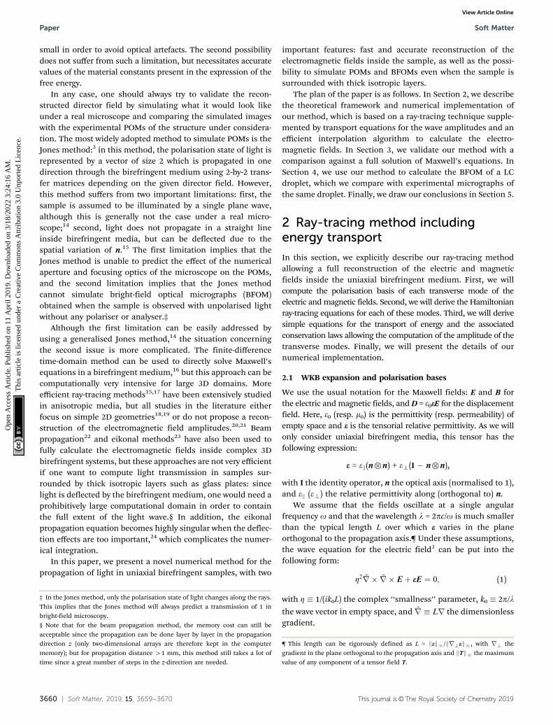
3.2 Results and discussion

Fig. 6 shows two density plots of Sz/S0 computed with the FDTDmethod (Fig. 6a) and our ray-tracing method (Fig. 6b). Theagreement between the two methods is visually very good,especially for the low-intensity elongated bands near the verticalboundaries of the computational domain. Note that the contrastof these bands is not due to an exchange of energy between theextraordinary and ordinary waves (which we neglected in Section2.3), but is simply caused by interference between these twowaves. This interference is possible because the polarisation ofan extraordinary ray at a given point is not orthogonal tothe polarisation of the associated ordinary ray at the same point(the directions of the wave vectors associated with both rays are

different since we have taken into account ray deflection). Hadwe neglected the deflection of the extraordinary rays – as in theJones method – no such interference would have been visible.

However, some differences between the ray-tracing andFDTD method can be seen in the small region R delimited bythe black dashed line of Fig. 6. This region was numericallyobtained by searching for all points where the relative errorbetween the FDTD solution and ray-tracing solution was morethan 25%. In this region, a sharp boundary between low andhigh intensity regions can be seen in the ray-tracing simulation,while the FDTD simulation is associated with a much smoothersolution. This sharp boundary corresponds to a caustic, whoseshape is similar to the one described schematically in Fig. 4.The sharp increase of intensity is due to an artificial divergence ofthe electric and magnetic field on the caustic itself, where thegeometrical spreading q can be shown to become zero.24 Since nosuch divergence is present in the exact solution of Maxwell’sequations, this means that our method is highly inaccurate nearcaustics – a problem which is common to all ray-based methods.24

Nevertheless, the good agreement between our method andthe FDTD method is quickly retrieved outside the domain R,whose extent is rather limited. This can be directly confirmedby looking at the horizontal and vertical profiles of the Sz/S0

field. Two such profiles are presented in Fig. 7. In these graphs,the intersection between the profile lines and the region R isrepresented by gray areas. At the center of these gray areas, thedivergence of Sz can be clearly seen, while outside these grayareas, the curves associated with the ray-tracing solutionquickly converge to the curves associated with the FDTDsolution. In particular, good agreement is obtained inside thecaustic domain (but sufficiently far from the caustic itself),where multiple extraordinary rays contribute to the local valueof the Maxwell fields (as depicted in Fig. 4).

Up until this point, all our results were associated with atransverse periodicity P/2 = 10 mm, as indicated in Table 1.Since this periodicity corresponds to the typical length overwhich the director field varies, the associated amplitudefor the smallness parameter introduced in Section 2.1 is

Table 1 Values of the wavelength and the material constants for the setupdescribed in Fig. 5. niso corresponds to the optical index of the isotropicdomain, and n>(n8) corresponds to the ordinary (extraordinary) index ofthe cholesteric domain

l P niso n> n8

0.5 mm 20 mm 1 1.45 1.55

Fig. 6 Density plot of the renormalised intensity Sz/S0 obtained with theFDTD method (a) and our ray-tracing method (b). The black dashed linedelimits a domain R where the typical relative error between the FDTDsolution and the ray-tracing solution is more than 25%.

Soft Matter Paper

Ope

n A

cces

s A

rtic

le. P

ublis

hed

on 1

1 A

pril

2019

. Dow

nloa

ded

on 3

/18/

2022

3:2

4:16

AM

. T

his

artic

le is

lice

nsed

und

er a

Cre

ativ

e C

omm

ons

Attr

ibut

ion

3.0

Unp

orte

d L

icen

ce.

View Article Online

3666 | Soft Matter, 2019, 15, 3659--3670 This journal is©The Royal Society of Chemistry 2019

|Z| � pl/P E 0.15. To determine how the accuracy of ourmethod varies with |Z|, we reproduced the same numericalexperiments as above with different values of pitch, whilekeeping the other parameters constant and using a scaledmesh of dimensions {P/2, P} in the {x,z} directions.

Whatever the value of the cholesteric pitch, we found that thetypical lateral extent of the branches defining the domain R isalways around 2l–4l, which means that our method allows us tolocalize the expansion error around the caustics, while keeping goodconvergence properties far from the caustics. In particular, weget an even better agreement with FDTD than in Fig. 6 and 7when the cholesteric pitch is greater than 20 mm, because themeshes associated with these systems are much bigger than thewavelength – and therefore much bigger than the typical lateralextent of the high-inaccuracy region R.

Conversely, the agreement between FDTD and ray-tracingbecomes less satisfactory for small cholesteric pitches: when|Z|� pl/P = 0.3, the mesh size becomes comparable to the lateralextent of the high-inaccuracy region, which means that theconvergence error is becoming global. This critical point corre-sponds to a periodicity length of 5 mm, which corresponds hereto ten times the wavelength. For even lower periodicity length,our method is not applicable anymore and a full solution ofMaxwell’s equations using FDTD must be envisioned.

On a similar line, we also noticed that the caustics werealways appearing at a critical vertical position zc scaling linearlywith the cholesteric pitch. This scaling can be theoreticallyexplained by directly computing the analytical expression of zc

for the system considered here:

zc ¼Pn?

4

ffiffiffiffiffiffiffiffiffiffiffiffiffiffiffiffiffiffiffiffiffiffiffiffink� �2� n?½ �2

q : (17)

The proof of this formula is available in Section S5 of the ESI.†Note that eqn (17) is only valid for positive birefringence(for negative birefringence, it needs to be adapted by switchingthe variables n8 and n>). This formula can be used to deter-mine if caustics are present or not in arbitrary birefringentslabs by replacing P/4 with the typical distance L over which thedirector switches from a vertical orientation to a horizontalorientation. For sufficiently thin samples (thickness smallerthan zc), caustics are not present in the birefringent slab andtherefore do not ‘‘pollute’’ the simulated fields with a divergingamplitude.

Finally, let us conclude this section by pointing out that ourimproved ray-tracing method is massively faster than the FDTDmethod. This can be directly checked by the running timesof both methods. As a typical example, the running timesassociated with the results of Fig. 6 and 7 are 4 s for ourmethod and around 1 h for FDTD. These running times wereobtained on a state-of-the-art desktop computer (6 multi-threaded cores cadenced at 3.5 GHz). Here, the high computa-tional cost of FDTD is simply explained by the high density ofthe mesh necessary to get an accurate solution: the wavelengthis much smaller than the typical size of our system, whichmeans that a few millions of points are necessary if we impose aratio of 75 vertices per wavelength. When a third dimension isadded to the system (as in the next section), the computationalcost of FDTD becomes prohibitive if the considered system islarge. Since our method works well for these large systems(small expansion parameter Z), it can be adopted as a replace-ment for FDTD.

4 Application to the visualisationof liquid crystal droplets

In this section, we show how our method is able to predict thebright-field optical micrographs (BFOMs) of liquid crystal dropletsas observed under a microscope when using unpolarised lightwithout any polariser and analyser – something that the Jonesmethod is unable to address. We first detail the experimental andnumerical setup used, and then present and discuss our results.

4.1 Experimental setup

We focused on one particular type of liquid crystal droplet,namely twisted bipolar droplets obtained at the thermo-dynamic coexistence between the nematic and isotropic phase.Twisted bipolar droplets are characterised by their planaranchoring (the molecules prefer to align parallel to the surfaceof the droplet), the existence of two diametrically opposedtopological defects of rank +1 (in agreement with the Poin-care–Hopf theorem applied to a sphere), and a double twistinternal structure for the director field of the droplet. This lastcharacteristic can be experimentally induced either by using acholesteric liquid crystal (in which case the director field has aspontaneous twist of fixed handedness) or an achiral nematicliquid crystal in which twist elastic deformations cost a negli-gible amount of free energy in comparison to splay and/or bend

Fig. 7 (a) Vertical profile of Sz/S0 over the line x = 0 mm. (b) Horizontalprofile of Sz/S0 over the line z = 19.5 mm. The legend of (a) also applies for(b). The gray regions correspond to the intersection of the domain R ofFig. 6b with the profile line.

Paper Soft Matter

Ope

n A

cces

s A

rtic

le. P

ublis

hed

on 1

1 A

pril

2019

. Dow

nloa

ded

on 3

/18/

2022

3:2

4:16

AM

. T

his

artic

le is

lice

nsed

und

er a

Cre

ativ

e C

omm

ons

Attr

ibut

ion

3.0

Unp

orte

d L

icen

ce.

View Article Online

This journal is©The Royal Society of Chemistry 2019 Soft Matter, 2019, 15, 3659--3670 | 3667

elastic deformations34 (in which case the director field prefers tobe twisted in order to decrease the energy of the surface defects).In the latter case, the twist can be left-handed or right-handedwith a 50/50 probability since it is due to energetically-inducedspontaneous symmetry breaking in an achiral system.

In our experiment, we exploited this spontaneous symmetrybreaking by using a lyotropic chromonic suspension of SunsetYellow FCF (SSY) in water with a mass fraction 29 wt%. Inconfined geometries filled with this mixture – such as thedroplets studied here – a twist can be observed because of thegiant elastic anisotropy of SSY suspensions, as reported byseveral authors.35–38 The protocol to prepare the sample andcreate twisted bipolar droplets was already described in a pre-vious article.38 Briefly, an aqueous suspension of SSY was con-tained between two parallel glass plates separated by nylon wiresof calibrated diameter 110 mm. The glass plates of the samplewere spin-coated beforehand with polyvinyl alcohol (PVA) andannealed at 120 1C in order to favor wetting of the sample plateby the isotropic phase of the SSY suspension. Once filled, thesample was sealed with UV glue and sandwiched by two trans-parent ovens separately regulated within 0.01 1C. A detaileddescription of these ovens is available in ref. 39. Note that twothin layers of glycerol were added between the sample and theovens in order to improve the thermal contact.

The sample was observed through the objective of a Leicamicroscope under bright-field illumination conditions (halogenlamp producing unpolarised white light, Kohler illuminationsetup allowing us to uniformly light the sample, no polariser andanalyser). Note that the condenser diaphragm of the microscopewas closed as much as possible in order to get normal illumina-tion on the sample (which is assumed in our numerical method).The temperatures of the ovens were adjusted to be inside thecoexistence range between the nematic and isotropic phase ofthe SSY sample. Thanks to the surface treatment of the sampleplate, the nematic domains dewetted the walls and formeddroplets in the bulk of the sample. The radius of the observeddroplets was then adjusted to be typically R E 25 mm bychanging the temperature of the ovens while staying inside thecoexistence range. By setting slightly different temperatures forthe top and bottom ovens, we noticed that the droplets formingin the sample only have two possible orientations: parallel ororthogonal to the induced vertical temperature gradient. Wechose to focus only on droplets with the polar axis orthogonal tothe view direction by centering the sample stage appropriately.

Optical micrographs of the droplets were captured thanks toa CCD camera (C4742, Hamamatsu). Note that the incidentunpolarised light was filtered using a red bandpass filter(l E 633 nm) in order to optimize the contrast of the micro-graphs. Since our goal is to study light deviation effects in thedroplets, we systematically saved for each micrograph thevertical shift of the sample stage with respect to a referenceposition where the droplet is well-focused.

4.2 Numerical setup

The first step to numerically reconstruct the optical micro-graphs of the twisted bipolar droplets was to compute the

director field associated with the observed SSY droplets.This was done using a trust-region finite-element minimisation(TR-FEM) of the total free energy of a spherical droplet withR = 25 mm. The details of this algorithm are given in anotherpaper.12 Briefly, we assume that the anchoring strength at thenematic/isotropic interface is finite, which implies that thepolar defects of the twisted bipolar droplets are only virtual(i.e. the Frank elastic energy stays finite near these defects).This allows us to neglect variations of the scalar order para-meter and write the total free energy F[n] of the droplet as:

F[n] = Ff[n] + Fs[n]

In this equation, Ff[n] corresponds to the Frank free energy,whose expression – given in the previous citation – depends onthe director field and on the elastic constants K1,2,3,4 respec-tively associated with splay, twist, bend, and Gauss/double twistdeformations. The second term Fs[n] corresponds to the con-tribution of the anchoring potential on the nematic/isotropicinterface, and its expression is given by:

Fs½n� ¼ð

S

K1

lan � vð Þ2dS

Here, la = K1/Wa is the anchoring length and Wa is the anchoringstrength. Our TR-FEM algorithm allows us to iteratively mini-mize a discretised version of F[n] with finite elements using anefficient null space factorisation of the gradient and Hessian ofthe free energy and a robust calculation of the solution updatewhich always decreases the energy and converges quadraticallynear a minimum of F[n]. We applied this algorithm to the caseof SSY droplets by using the values of the material constantsgiven in Table 2. The resulting director field, obtained on amesh with approximately 2� 106 vertices, is presented in Fig. 8.

Once the director field was computed, we used it in our ray-tracing code to propagate light through the system described inthe previous section, including all the isotropic layers asso-ciated with the transparent ovens and the sample plates. Sincewe are only interested in the final micrographs and not in thebulk data of the Maxwell fields, we skipped step (A2.3) of ouralgorithm (see Section 2.4) and simply propagated forward therays through the system using the values of the materialconstants in Table 2.

Table 2 Values of the relevant material constants for the system ofSection 4. The Frank elastic constants K1,2,3 and refractive indices n>,8,iso

in the SSY suspension were measured by Zhou et al.29 The K4 constant wasestimated using the theoretical formula of Nehring and Saupe.30 Theanchoring length la at the nematic/isotropic interface was never measuredin SSY so we took a similar value to that in cyanobiphenyls,31 and wechecked that the computed micrographs were not changing much whenapplying a factor 0.5–2 to this value. The values of the refractive index ofthe glass, glycerol and water layers were obtained from tabulated data32,33

K2/K1 K3/K1 K4/K1 la l

0.161 1.43 0.58 3 mm 633 nm

nglass nglycerol nwater niso n> n8

1.52 1.47 1.33 1.43 1.47 1.41

Soft Matter Paper

Ope

n A

cces

s A

rtic

le. P

ublis

hed

on 1

1 A

pril

2019

. Dow

nloa

ded

on 3

/18/

2022

3:2

4:16

AM

. T

his

artic

le is

lice

nsed

und

er a

Cre

ativ

e C

omm

ons

Attr

ibut

ion

3.0

Unp

orte

d L

icen

ce.

View Article Online

3668 | Soft Matter, 2019, 15, 3659--3670 This journal is©The Royal Society of Chemistry 2019

Under a real microscope, optical micrographs are obtainedby propagating light through the objective to the final screen(here, the CCD image sensor). In our numerical method, weassume that the objective can be represented by an ideal lens,in which case the final screen P is conjugated through the lensto a virtual plane P0, which we call the back-focal plane. Theseplanes are schematised in Fig. 9. Since we assumed that the

lens is ideal, the final intensity field on the plane P is perfectlyequivalent (with a scaling transformation) to the intensityfield on the virtual plane P0, which can be obtained bypropagating backward the output rays as if the whole spacewas filled with air (dashed trajectories in Fig. 9). For thisreason, we calculated the optical micrographs by combiningall contributions of the ray families on the back-focal planeafter propagating the rays forward through the system andbackward to the virtual plane P0. Since an input polarisationmust be specified in our method, the final BFOM is obtainedby averaging incoherently the simulated POMs over all possi-ble input polarisations.

4.3 Results and discussion

A few observed and simulated BFOMs are presented inFig. 10a and b for different vertical positions of the back-focal plane P0. The same contrast setting (Sz/S0 between0.5 and 1.5) was applied to all micrographs for ease ofcomparison. As can been seen, the simulated micrographscorrectly predict the existence of the almond-shaped highintensity region at the center of the droplet, which opens upand expands when the back-focal plane is moved upward. Letus remark that our first attempt to simulate the BFOMsof Fig. 10 was unsuccessful because we initially neglectedthe presence of all the additional isotropic layers associatedwith the sample plates and the transparent ovens ofthe experimental setup: in this simplified situation, the simu-lated micrographs were much more uniform (inexistentalmond-shaped high intensity region) and therefore verydifferent from the observations. The fact that the micrographshave a much sharper contrast when including the isotropiclayers in the simulation can be interpreted as an amplificationof the deflection effects on the back-focal plane P0 due tolight refraction at the boundaries of the isotropic layers(see Fig. 9).

Although the agreement between the simulated andobserved BFOMs is good, some discrepancies are clearlyvisible, especially outside the droplet and near its boundary.First, it is easy to see that the simulated interference ringsoutside the droplet are thicker and of higher contrast than inthe experimental images. This discrepancy is probably due tothe fact that we neglected all reflected rays on the boundaryof the droplet. Second, optical artefacts are visible near thepolar defects (left and right side of the droplet) when Dz o 0 inFig. 10. These artefacts are associated with the presenceof caustics, where the reconstructed Maxwell fields are highlyinaccurate as shown in the previous section. Last, thecrescent-shaped high intensity regions visible in the experi-mental micrographs when Dz 4 0 are much thinner in thesimulated micrographs. This discrepancy is not due to thepresence of caustics (which can be directly checked inour result files by counting the number of rays arriving atone point of the micrograph); the most likely source of error isthat the effective birefringence Dneff introduced in Section 2.3is vanishingly small near the boundary of the droplet,

Fig. 8 Director field of an SSY droplet with R = 25 mm on three sliceplanes and on the droplet surface. Here, y is the polar axis associated witha rotational invariance and z is the direction of propagation of light in theray-tracing simulation.

Fig. 9 In this figure, we illustrate how two different rays (brown and greentrajectories, respectively associated with extraordinary and ordinary rays)are recombined at a point (O) of the final screen P after passing throughthe ideal lens L. Since this lens is assumed ideal, the intensity data at point(O) is perfectly equivalent to the intensity data at the conjugate point (O0)

on the back-focal plane P0. For this reason, we calculate micrographs bypropagating backward the rays to this virtual plane (dashed trajectories).Here, we assumed that the droplet is embedded in a single isotropicmedium, but our approach can be easily generalized to more complexsetups.

Paper Soft Matter

Ope

n A

cces

s A

rtic

le. P

ublis

hed

on 1

1 A

pril

2019

. Dow

nloa

ded

on 3

/18/

2022

3:2

4:16

AM

. T

his

artic

le is

lice

nsed

und

er a

Cre

ativ

e C

omm

ons

Attr

ibut

ion

3.0

Unp

orte

d L

icen

ce.

View Article Online

This journal is©The Royal Society of Chemistry 2019 Soft Matter, 2019, 15, 3659--3670 | 3669

where the director is almost parallel to the propagation axis.This implies that one of the main assumptions of our code(Mauguin number much bigger than 1) is broken near thedroplet boundary, which explains the difference between thesimulated and observed BFOMs near the crescent-shaped highintensity regions described above.

Nevertheless, we checked that the Mauguin number isreasonably high enough (Z10) at the center of the dropletand that the WKB expansion parameter |Z| E 1/(2k0R) is smallenough (B0.002), which explains why our ray-tracing method isrobust enough to qualitatively predict the correct alternation ofdark and bright bands in all micrographs. It should be notedthat additional insight into the structure of the micrographscan be obtained by looking at the deflection maps of theextraordinary and ordinary rays, defined as the differenceDr(a) between the actual end point of a ray r(a) (a = e or o)and the virtual end point which would be obtained if there wereno deflection of this ray. These deflection maps are plotted inthe two bottom rows of Fig. 10. The ordinary deflection mapalways has rotational symmetry (which is expected since theordinary index is constant inside the spherical droplet) andpoints outward for Dz o 0 and inward for Dz 4 0, whichexplains the presence of interference rings outside the dropletwhen Dz o 0 and the dark bands near the boundary of thedroplet when Dz 4 0. The extraordinary deflection map has C2

symmetry (as expected because of the bipolar and twistednature of the director field) and points inward for Dz o 0and outward for Dz 4 0, which explains why the almond-shaped high intensity region opens up and expands when Dzincreases. Finally, we should clarify exactly what we meant by a

‘‘well-focused droplet’’ when defining the reference position ofthe back focal plane P0 (Dz = 0 in Fig. 10): here, ‘‘well-focused’’simply means that the average deflection amplitude of theordinary rays is minimal (as can be visually checked in Fig. 10d).

5 Conclusion

To summarize, we presented an improved ray-tracing methodallowing one to fully reconstruct the phase, polarisation andamplitude of the optical field inside a uniaxial birefringentmedium. We demonstrated that this method is extremely fastin comparison to a full resolution of Maxwell’s equations, andshowed that the calculated solutions are accurate far fromcaustics, which only formed when the sample thickness isgreater than a critical value. Finally, we showed how ourmethod can be used to simulate bright-field optical micro-graphs of birefringent samples as seen under a microscope,with good agreement with experimental micrographs. Ourmethod is thus able to address one of the main limitation ofthe Jones method, namely the inability to take into account raydeflection and simulate light propagation under bright-fieldillumination conditions. Contrary to the numerical methodsmentioned in Section 1 (finite difference time domain, beampropagation method, eikonal differential equation. . .), ourmethod is also able to support complex setups with thickisotropic layers. The main reason for this is that we do nothave to solve a set of partial differential equations, we only haveto propagate rays and reconstruct the electric fields alongthese rays.

Fig. 10 Experimental (a) and simulated (b) BFOMs of a SSY droplet with R = 25 mm, for different vertical shift Dz of the back-focal plane P0 with respect toa reference position associated with a well-focused droplet (fourth column). The two bottom rows represent the deflection maps of the extraordinary (c)and ordinary (d) rays. The color scale is associated with the amplitude of deflection. Note that the Jones method is unable to simulate these BFOMs sinceit always predicts a transmission of 1 under bright-field illumination conditions.

Soft Matter Paper

Ope

n A

cces

s A

rtic

le. P

ublis

hed

on 1

1 A

pril

2019

. Dow

nloa

ded

on 3

/18/

2022

3:2

4:16

AM

. T

his

artic

le is

lice

nsed

und

er a

Cre

ativ

e C

omm

ons

Attr

ibut

ion

3.0

Unp

orte

d L

icen

ce.

View Article Online

3670 | Soft Matter, 2019, 15, 3659--3670 This journal is©The Royal Society of Chemistry 2019

Note that the simplicity and effectiveness of our method arelargely due to the fact that we neglected any exchange of energybetween the extraordinary and ordinary modes. This assump-tion is only valid if the Mauguin number is much bigger than 1.As discussed in Sections 3 and 4, this was mainly the case forthe systems studied here. In the future, it would be interestingto further improve our numerical method by relaxing thisassumption and deriving general transport equations for theamplitude of the extraordinary and ordinary modes outsidethe adiabatic regime. Such a generalised method could then beapplied to highly chiral birefringent systems, in which the twistof the polarisation is non-negligible everywhere in the sample.

On a parallel note, although our method was mainly appliedto the calculation of optical micrographs, one could imagine anumber of other applications. For example, our method could beused to analyze the diffraction patterns of the LC-based diffrac-tion gratings mentioned in the introduction, by setting the finaltarget plane of our method to the output plane of the LC layer,and then applying the usual far-field formula. The optical prop-erties of flat LC diffractive lenses40 could also be analyzed eitherby using the ray trajectories computed by our method or by usingthe reconstructed fields on the output surface of the LC layer.

Conflicts of interest

There are no conflicts to declare.

Acknowledgements

The authors warmly thank P. Oswald for giving access to theexperimental setup used in this paper. Funding is acknowl-edged from the ARSS (Javna Agencija za Raziskovalno DejavnostRS) through grants P1-0099 and L1-8135, and from theEuropean Union’s Horizon 2020 programme through the MarieSkłodowska-Curie grant agreement No. 834256.

References

1 P. Oswald and P. Pieranski, Nematic and cholesteric liquidcrystals: concepts and physical properties illustrated by experi-ments, CRC Press, 2006.

2 P. Oswald and P. Pieranski, Smectic and columnar liquidcrystals: concepts and physical properties illustrated by experi-ments, CRC Press, 2006.

3 I.-C. Khoo, Liquid crystals: physical properties and nonlinear opticalphenomena, Wiley-Interscience, Hoboken, N.J., 2nd edn, 2007.

4 M. Humar, M. Ravnik, S. Pajk and I. Musevic, Nat. Photonics,2009, 3, 595–600.

5 P. J. Ackerman, Z. Qi, Y. Lin, C. W. Twombly, M. J. Laviada,Y. Lansac and I. I. Smalyukh, Sci. Rep., 2012, 2, 414.

6 I. Nys, K. Chen, J. Beeckman and K. Neyts, Adv. Opt. Mater.,2018, 6, 1701163.

7 M. Jiang, H. Yu, X. Feng, Y. Guo, I. Chaganava, T. Turiv,O. D. Lavrentovich and Q.-H. Wei, Adv. Opt. Mater., 2018,1800961.

8 Y. Tabe and H. Yokoyama, Langmuir, 1995, 11, 699–704.9 I. Smalyukh, Mol. Cryst. Liq. Cryst., 2007, 477, 23–41.

10 T. Lee, R. P. Trivedi and I. I. Smalyukh, Opt. Lett., 2010, 35,3447–3449.

11 M. Ravnik and S. Zumer, Liq. Cryst., 2009, 36, 1201–1214.12 G. Poy, F. Bunel and P. Oswald, Phys. Rev. E, 2017, 96, 012705.13 G. Posnjak, S. Copar and I. Musevic, Sci. Rep., 2016, 6, 26361.14 U. Mur, S. Copar, G. Posnjak, I. Musevic, M. Ravnik and

S. Zumer, Liq. Cryst., 2017, 44, 679–687.15 F. Grandjean, Bull. Soc. Fr. Mineral., 1919, 42, 42.16 A. F. Oskooi, D. Roundy, M. Ibanescu, P. Bermel, J. Joannopoulos

and S. G. Johnson, Comput. Phys. Commun., 2010, 181, 687–702.17 A. Joets and R. Ribotta, Opt. Commun., 1994, 107, 200–204.18 J. A. Kosmopoulos and H. M. Zenginoglou, Appl. Opt., 1987,

26, 1714.19 H. M. Zenginoglou and J. A. Kosmopoulos, Appl. Opt., 1989,

28, 3516.20 M. Sluijter, D. K. G. de Boer and J. J. M. Braat, J. Opt. Soc. Am.

A, 2008, 25, 1260.21 M. Sluijter, D. K. de Boer and H. P. Urbach, J. Opt. Soc. Am.

A, 2009, 26, 317.22 G. D. Ziogos and E. E. Kriezis, Opt. Quantum Electron., 2008,

40, 733–748.23 G. Panasyuk, J. Kelly, E. C. Gartland and D. W. Allender, Phys.

Rev. E: Stat., Nonlinear, Soft Matter Phys., 2003, 67, 041702.24 O. Runborg, Commun. Comput. Phys., 2007, 2, 827–880.25 R. B. Dingle and R. Dingle, Asymptotic expansions: their

derivation and interpretation, Academic Press, London,1973, vol. 48.

26 H. L. Ong, J. Appl. Phys., 1988, 64, 614–628.27 F. Lekien and J. Marsden, Int. J. Numer. Meth. Eng., 2005, 63,

455–471.28 A. Taflove and S. C. Hagness, Computational electrodynamics: the

finite-difference time-domain method, Artech house, 2005.29 S. Zhou, Y. A. Nastishin, M. M. Omelchenko, L. Tortora, V. G.

Nazarenko, O. P. Boiko, T. Ostapenko, T. Hu, C. C. Almasan,S. N. Sprunt, J. T. Gleeson and O. D. Lavrentovich, Phys. Rev.Lett., 2012, 109, 037801.

30 J. Nehring and A. Saupe, J. Chem. Phys., 1971, 54, 337–343.31 S. Faetti and V. Palleschi, Phys. Rev. A: At., Mol., Opt. Phys.,

1984, 30, 3241.32 M. Rubin, Sol. Energy Mater., 1985, 12, 275–288.33 J. Rheims, J. Koser and T. Wriedt, Meas. Sci. Technol., 1997,

8, 601–605.34 R. D. Williams, J. Phys. A: Math. Gen., 1986, 19, 3211.35 L. Tortora and O. D. Lavrentovich, Proc. Natl. Acad. Sci. U. S. A.,

2011, 108, 5163–5168.36 J. Jeong, Z. S. Davidson, P. J. Collings, T. C. Lubensky and

A. G. Yodh, Proc. Natl. Acad. Sci. U. S. A., 2014, 111, 1742–1747.37 K. Nayani, R. Chang, J. Fu, P. W. Ellis, A. Fernandez-Nieves,

J. O. Park and M. Srinivasarao, Nat. Commun., 2015, 6, 8067.38 J. Ignes-Mullol, G. Poy and P. Oswald, Phys. Rev. Lett., 2016,

117, 057801.39 P. Oswald and A. Dequidt, Phys. Rev. Lett., 2008, 100, 217802.40 P. Valley, D. L. Mathine, M. R. Dodge, J. Schwiegerling,

G. Peyman and N. Peyghambarian, Opt. Lett., 2010, 35, 336–338.

Paper Soft Matter

Ope

n A

cces

s A

rtic

le. P

ublis

hed

on 1

1 A

pril

2019

. Dow

nloa

ded

on 3

/18/

2022

3:2

4:16

AM

. T

his

artic

le is

lice

nsed

und

er a

Cre

ativ

e C

omm

ons

Attr

ibut

ion

3.0

Unp

orte

d L

icen

ce.

View Article Online