voltage fluctuation in industrial network and compensation measures
TRANSCRIPT

8/12/2019 Voltage fluctuation in industrial network and compensation measures
http://slidepdf.com/reader/full/voltage-fluctuation-in-industrial-network-and-compensation-measures 1/156
UNIVERSITY OF LJUBLJANA
Faculty of Electrical Engineering
Ljubiša Spasojević
VOLTAGE FLUCTUATION IN INDUSTRIALNETWORK AND COMPENSATION
MEASURES
DOCTORAL DISSERTATION
Ljubljana, 2014

8/12/2019 Voltage fluctuation in industrial network and compensation measures
http://slidepdf.com/reader/full/voltage-fluctuation-in-industrial-network-and-compensation-measures 2/156

8/12/2019 Voltage fluctuation in industrial network and compensation measures
http://slidepdf.com/reader/full/voltage-fluctuation-in-industrial-network-and-compensation-measures 3/156

8/12/2019 Voltage fluctuation in industrial network and compensation measures
http://slidepdf.com/reader/full/voltage-fluctuation-in-industrial-network-and-compensation-measures 4/156

8/12/2019 Voltage fluctuation in industrial network and compensation measures
http://slidepdf.com/reader/full/voltage-fluctuation-in-industrial-network-and-compensation-measures 5/156
UNIVERSITY OF LJUBLJANA
Faculty of Electrical Engineering
Ljubiša Spasojević
VOLTAGE FLUCTUATION IN INDUSTRIALNETWORK AND COMPENSATION
MEASURES
DOCTORAL DISSERTATION
Mentor: prof. dr. Igor Papič
Ljubljana 2014

8/12/2019 Voltage fluctuation in industrial network and compensation measures
http://slidepdf.com/reader/full/voltage-fluctuation-in-industrial-network-and-compensation-measures 6/156
8/12/2019 Voltage fluctuation in industrial network and compensation measures
http://slidepdf.com/reader/full/voltage-fluctuation-in-industrial-network-and-compensation-measures 7/156
UNIVERZA V LJUBLJANI
Fakulteta za elektrotehniko
Ljubiša Spasojević
KOLEBANJE NAPETOSTI VINDUSTRIJSKEM OMREŽJU IN
KOMPENZACIJSKI UKREPI
DOKTORSKA DISERTACIJA
Mentor: prof. dr. Igor Papič
Ljubljana, 2014

8/12/2019 Voltage fluctuation in industrial network and compensation measures
http://slidepdf.com/reader/full/voltage-fluctuation-in-industrial-network-and-compensation-measures 8/156

8/12/2019 Voltage fluctuation in industrial network and compensation measures
http://slidepdf.com/reader/full/voltage-fluctuation-in-industrial-network-and-compensation-measures 9/156
To my father Milan and my mother Zora

8/12/2019 Voltage fluctuation in industrial network and compensation measures
http://slidepdf.com/reader/full/voltage-fluctuation-in-industrial-network-and-compensation-measures 10/156

8/12/2019 Voltage fluctuation in industrial network and compensation measures
http://slidepdf.com/reader/full/voltage-fluctuation-in-industrial-network-and-compensation-measures 11/156

8/12/2019 Voltage fluctuation in industrial network and compensation measures
http://slidepdf.com/reader/full/voltage-fluctuation-in-industrial-network-and-compensation-measures 12/156

8/12/2019 Voltage fluctuation in industrial network and compensation measures
http://slidepdf.com/reader/full/voltage-fluctuation-in-industrial-network-and-compensation-measures 13/156

8/12/2019 Voltage fluctuation in industrial network and compensation measures
http://slidepdf.com/reader/full/voltage-fluctuation-in-industrial-network-and-compensation-measures 14/156

8/12/2019 Voltage fluctuation in industrial network and compensation measures
http://slidepdf.com/reader/full/voltage-fluctuation-in-industrial-network-and-compensation-measures 15/156
Ljubiša Spasojević Doctoral dissertation
Content
LIST OF ABBREVIATIONS AND SYMBOLS............................................................................................................... 11
ABSTRACT ............................................................................................................................................................ 17
RAZŠIRJENI POVZETEK .......................................................................................................................................... 21
1. INTRODUCTION ........................................................................................................................................... 29
1.1 SUBJECT OF THE DOCTORAL DISSERTATION .............................................................................................................. 30
1.2 CONTRIBUTION TO SCIENCE .................................................................................................................................. 31
2 POWER QUALITY ......................................................................................................................................... 33
2.1 STANDARD EN 50160 ....................................................................................................................................... 33
Frequency of the supply voltage .................................................................. ...................................................... 34
Declared supply voltage .................................................................................................................................... 34
Voltage deviation .............................................................................................................................................. 34
Voltage dip ........................................................................................................................................................ 35
Interruption of voltage supply ........................................................................................................................... 36
Temporary overvoltage between live conductors and earth ........................................................ ..................... 36
Transient overvoltage between live conductors and earth ............................................................................... 37
Voltage unbalance .................................................................. .................................................................. ......... 38
Rapid voltage fluctuations ................................................................ ................................................................. 39
3 FLICKER ....................................................................................................................................................... 41
3.1 OCCURRENCE OF FLICKER AND FLICKER SOURCES ...................................................................................................... 42
Occurrence of flicker .......................................................................................................................................... 43
Arc furnace ............................................................................ ................................................................... ......... 45
Welding machine ............................................................................................................................................... 46
Wind turbines .................................................................................................................................................... 46
3.2 ESTIMATE OF THE FLICKER LEVEL ........................................................................................................................... 46
3.3 FLICKERMETER .................................................................................................................................................. 48
Block 1 – input voltage adapter ................................................................... ...................................................... 49
Block 2 - squaring multiplier .............................................................................................................................. 49
Block 3 – filters .................................................................................................................................................. 50
Block 4 - non-linear variance estimator .................................................................. ........................................... 51
Block 5 - statistical calculation block ................................................................................................................. 52
4 ELECTRIC ARC FURNACE .............................................................................................................................. 55 4.1 FURNACE WITH A DIRECT ELECTRICAL ARC ............................................................................................................... 55
4.2 INDIRECT ARC FURNACES ..................................................................................................................................... 57
4.3 FURNACE WITH A SUBMERGED ARC ........................................................................................................................ 57
4.4 ELECTRIC ARC .................................................................................................................................................... 58 Electric arc of direct current .............................................................................................................................. 59
Electric arc of alternating current ................................................................ ...................................................... 62
5 DYNAMIC REACTIVE-POWER COMPENSATION ............................................................................................ 65
5.1 FLEXIBLE ALTERNATING-CURRENT TRANSMISSION SYSTEM .......................................................................................... 65
5.2 STATIC VAR COMPENSATOR ................................................................................................................................ 67
FC-TCR structure ................................................................................................................................................ 67
6 THE MODELLING OF ELECTRIC ARC FURNACES ............................................................................................ 73
6.1 REPRESENTATIVE SAMPLES OF VOLTAGE AND CURRENT ............................................................................................. 74
The Selection of Representative Samples .......................................................................................................... 75
6.2 MODEL OF THE FLICKERMETER .............................................................................................................................. 80 Testing of S(t) .............................................................. .................................................................. ..................... 80
9

8/12/2019 Voltage fluctuation in industrial network and compensation measures
http://slidepdf.com/reader/full/voltage-fluctuation-in-industrial-network-and-compensation-measures 16/156
Ljubiša Spasojević Doctoral dissertation
Testing of the Pst ................................................................................................................................................ 82
6.3 BASIC CONCEPT OF THE MODEL OF THE ELECTRIC ARC FURNACE ................................................................................ 82
System Configuration ........................................................................................................................................ 84
Modeling the Electrical Arc Length.................................................................................................................... 86
Calculation of the Voltage Envelope ................................................................................................................. 87
6.4 THE RESULTS OF THE SIMULATION ........................................................................................................................ 88
7 DEVELOPING THE CONTROL ALGORITHM ................................................................................................... 95
7.1 VECTOR ILLUSTRATION OF THREE-PHASE QUANTITIES ................................................................................................ 95
Instantaneous active and reactive power ......................................................................................................... 98
7.2 COMPENSATION PRINCIPLE AND MATHEMATICAL MODEL OF TCR .............................................................................. 100
7.3 CONTROLLER DESIGN ........................................................................................................................................ 103
Transfer function of the P controller ............................................................................................................... 105
7.4 MODEL TESTING .............................................................................................................................................. 107
The static analysis .......................................................................................................................................... 107
The dynamic analysis ...................................................................................................................................... 109
7.5 THE SIMULATION RESULTS ................................................................................................................................. 111
The system configuration ................................................................................................................................ 112
7.6 MODELLING OF THE ELECTRIC-ARC LENGTH USING SINUSOIDAL FUNCTION ................................................................... 114 Simulations without a connected SVC ............................................................................................................. 114
Simulations with connected SVC ..................................................................................................................... 120
Reactive power and flicker-regulation mode .................................................................................................. 120
Voltage-regulation mode ................................................................................................................................ 127
7.7 MODELLING OF THE ELECTRIC-ARC LENGTH USING A SIGNAL THAT INVOLVES THE ALL-IMPORTANT FREQUENCIES FOR FLICKER 130
Simulations without the connected SVC .......................................................................................................... 130
Reactive power and flicker regulation mode ................................................................ ................................... 135
Voltage-regulation mode ................................................................................................................................ 139
7.8 SIMULATION WITH ANOTHER FREQUENCY SPECTRUM .............................................................................................. 141
7.9 ASSESSMENT OF THE CONTROLLER CHARACTERISTICS .............................................................................................. 142
8 CONCLUSION ............................................................................................................................................ 145
9 REFERENCES: ............................................................................................................................................ 147
10

8/12/2019 Voltage fluctuation in industrial network and compensation measures
http://slidepdf.com/reader/full/voltage-fluctuation-in-industrial-network-and-compensation-measures 17/156
Ljubiša Spasojević Doctoral dissertation
List of abbreviations and symbols
List of used abbreviations
AC Alternating current BESS Battery energy storage system DC Direct current DFT Discrete Fourier transformation EAF Electric arc furnace EMC Electromagnetic compatibility FACTS Flexible Alternating Current Transmission System FC Fixed-capacitor
FC-
TCR Fixed-
capacitor Thyristor Controlled Reactor
FFT Fast Fourier transformationIPFC Interline Power Flow Controller MV Medium-voltagePCC Point of common couplingSRCS Synchronous rotation coordinate systemSSG Static Synchronous Generator SSSC Static Synchronous Series Capacitor STATCOM Static Synchronous Compensator
SVC
Static VAr compensator
TCPST Thyristor-controlled phase-shifting transformersTCR Thyristor Controlled Reactor TCR Thyristor Controlled Reactor TCSC Thyristor Controlled Series Capacitor TCSR Thyristor Controlled Series Reactor TSSC Thyristor Switched Series Capacitor TSSR Thyristor Switched Series Reactor UPFC Unified Power Flow Controller
Symbols used in section 3
f b Basic frequency of the voltage
f m Frequency of modulation
m Factor of modulation
P inst Instantaneous flicker sensation
P inst, max Maximum instantaneous flicker sensation
P lt Long-term flicker index
P st Short-term flicker index
t Time
U(t) Basic amplitude of the voltage
11

8/12/2019 Voltage fluctuation in industrial network and compensation measures
http://slidepdf.com/reader/full/voltage-fluctuation-in-industrial-network-and-compensation-measures 18/156
Ljubiša Spasojević Doctoral dissertation
ω Angular frequency
Symbols used in section 4
∆B Correction factor due to the Schottky effect A, B, C, D Constants
E arc Electric field in the arc
f FrequencyI arc RMS value of arc currenti arc Waveforms of the arc current
J Emission density
l Arc length M Frist characteristic constant that depend on type of material
N
Second characteristicconstant that depend on type of material
T Temperature of cathode
U arc RMS value of arc voltage
u arc Waveforms of the arc voltage
U -I Voltage-Current characteristic
Symbols used in section 5
B TCR Reactive admittance (susceptance) of the TCR
cosφ Power factor
i(t) Instantaneous current
I FC Root-mean-square values of constant capacitive reactive current
I rms Root-mean-square values of i
I SVC Root-mean-square values of total reactive power current
I TCR Variable inductive reactive current
L Inductance of the thyristor-controlled reactor
U Peak value of the applied voltage
u(t) Instantaneous voltage
U rms
Root-mean-
square values ofu
u S (t) Instantaneous source voltageα Thyristor firing angle
ω Angular frequency of the supply voltage
Symbols used in section 6
∆u Voltage drop
A Sum of the anode and cathode voltage dropsAm
Amplitude
B Voltage drop per unit of the arc length
12

8/12/2019 Voltage fluctuation in industrial network and compensation measures
http://slidepdf.com/reader/full/voltage-fluctuation-in-industrial-network-and-compensation-measures 19/156
Ljubiša Spasojević Doctoral dissertation
C, D Constants
F(f, A, φ) Function for control of the variable voltage source
f s Sampling frequency
G
Gaini A Instantaneous value of arc current i RS Representative sample of the current
k Ratio between the arc voltage’s threshold value U AT (l ) at length l , andU AT (l 0 ) at the reference length l 0
l Length of the arc
l 0 Reference length of the arc
L C Cable inductance
L f Furnace inductance
L LSC Short-circuit inductance
p(t) Characteristic signal with frequencies from 1
Hz to 35 Hz of electric
arc furnace
p'(t) Characteristic signal of electric arc furnace, fingerprint of electric arcfurnace
P 1 Active power of the selected representative sample
P m Mean values of the active power of the ten-minute measured signal
P s Active power of the one-second sample
P sim Active power obtained by simulation
P st Flicker level of the ten-minute measured signal
P st, sim Flicker level obtained by simulation
P st, s Flicker levels of one-second sample
P st,1 Flicker levels of the selected representative sample
Q 1 Reactive power of the selected representative sample
Q m Mean values of the reactive power of the ten-minute measured signal
Q s Reactive power of the one-second sample
Q sim Reactive power obtained by simulation
r(t) Law of the arc-length variation
R C Cable resistance
R eq
Equivalent resistance
R f Furnace resistanceR LSC Short-circuit resistance
S(t) Instantaneous value of flicker
S” sc Short-circuit power at the 110-kv bus
T Total simulation time
u A Instantaneous value of arc voltage
u A Voltage at the point of the arc furnace’s connection to the network
u A0 Arc voltage corresponding to the reference length of the arc
U AT The threshold value to which the voltage tends for the reference
length of the arc
13

8/12/2019 Voltage fluctuation in industrial network and compensation measures
http://slidepdf.com/reader/full/voltage-fluctuation-in-industrial-network-and-compensation-measures 20/156
Ljubiša Spasojević Doctoral dissertation
u RS Representative sample of the voltage
X eq Equivalent reactance
φ Phase displacement of interharmonic
Symbols used in section 7
α Firing angle
b Variable factorBTCR Susceptance of the TCR cosφ Power factor
dq0, dq Direct quadrature zero transformations
F Control function of the controllable voltage sources F(s)tr Transfer functions of the system
i α α components of the current
i β β components of the current
i a_TCR , i b_TCR ,
i c_TCR Currents through the reactors in the star equivalent scheme
i ab , i bc , i ca Currents through the reactors in the delta equivalent scheme
i B Base values of the current
i d d components of the current
id’ d components of the current that flows into the TCR in p.u. iFC Currents of FC
il Load current
IL RMS value of the current through the reactor
i q q components of the current
iq’ q components of the current that flows into the TCR in p.u. iq’* Reference current
iqFC Reactive components of the FC current
iql Reactive component of the load current
iqs Reactive component of the system current
iqs
’*
Measured value of the reactive component of the total system currenti qs
iqSVC Reactive components of the current of SVC device
iqTCR Reactive component of the TCR current
is System currenti sa , i sb , i sc System currents, currents from the power system
iSVC Current of the SVC deviceiTCR Currents of TCR
Kp Gain of P controller
L Inductance of the TCRLa
, Lb
, Lc Inductance of inductor in star configuration
Lab, Lbc, Lca Inductance of inductor in delta configuration
14

8/12/2019 Voltage fluctuation in industrial network and compensation measures
http://slidepdf.com/reader/full/voltage-fluctuation-in-industrial-network-and-compensation-measures 21/156
Ljubiša Spasojević Doctoral dissertation
Lf inductance of the cable line between the furnace transformer and the
furnace electrodes
LLSC Short-circuit inductance
p Instantaneous active power in dq rotation coordinate system
P Proportional controllerPI Proportional–integral controller
Pst Short-term flicker index
q Instantaneous reactive power in dq rotation coordinate system qins Instantaneous values of the reactive powerRa, Rb, Rc Resistance of resistor in star configuration Rab, Rbc, Rca Resistance of resistor in delta configuration Rf Resistance of the cable line between the furnace transformer and the
furnace electrodes
RLSC
Short-circuit resistance
S’’sc Short-circuit power at the 110-kV bus
T Total simulation time
T dq Transformation matrix for dq transformations
TTCR Response time of the TCR
T αβ Transformation matrix for αβ transformations U RMS value of the connected voltage
u α α components of the voltage
u β β components of the voltage
u a , u b , u c , Phase-to-neutral voltages at the point of common coupling
u B Base values of the voltage
u d d components of the voltage
u d ’ d components of the voltage in p.u.
ud’ d components of the measured voltage at the SVC connection point
uMV Voltage at the MV level u q q components of the voltage
u q ’ q components of the voltage in p.u.
uq’ q components of the measured voltage at the SVC connection point
URMS
RMS voltage at the MV level
XL Maximum reactance of the TCR
Z B Base values of the impedance
αβ0, αβ αβ transformationsφ Angle between the voltage vector and the d-axes of the dq SRCS
ω Angular speed of the rotation coordinate system
ω b Synchronous angular speed of the fundamental network component
15

8/12/2019 Voltage fluctuation in industrial network and compensation measures
http://slidepdf.com/reader/full/voltage-fluctuation-in-industrial-network-and-compensation-measures 22/156

8/12/2019 Voltage fluctuation in industrial network and compensation measures
http://slidepdf.com/reader/full/voltage-fluctuation-in-industrial-network-and-compensation-measures 23/156
Ljubiša Spasojević Doctoral dissertation
Abstract
The main theme of this doctoral dissertation is the compensation of the negative impacts of
electric arc furnaces
(EAFs
)in a power system. Is generally known that an
EAF represents
a large consumer of electrical energy, which because of its nonlinear characteristics has astrong feedback influence on the power quality in the electric power system, and as suchrequires the installation of compensation devices. The development and design ofcompensation devices for the EAF is a major problem because of the non-linear electricalcharacteristics of the EAF. In the development and design process of compensating devicesan important role is played the simulation model of the EAF. In order to be able to developa cost-effective and at the same time very efficient compensating device we need to have
the most accurate simulation model of the EAF. The key contributions to science of this
doctoral dissertation are from the fields of the development and design of a real model of
an EAF and a control algorithm for the compensation device in order to eliminate thenegative impacts of the EAF on the power system.
This dissertation can be divided into two parts: first, is the theoretical part and, second, isthe research-development part of the work. The theoretical part includes the first 5chapters and in it is a theoretical presentation of the existing situation and issues, while the
research-development part of this work is included in the last three chapters, and in it is a
presentation of the results of the research work and the solutions for some existing issues.
In Chapter 2 is the basic structure of the power-quality concept (what the term 'powerquality' means and why it is necessary to define it ). On the basis of the standard EN 50160thirteen basic parameters are defined that are essential to the power quality. Theseparameters will be respected by consumers and by suppliers. For all 13 defined parametersthe minimum and maximum allowable values that must be followed are presented.
Chapter 3 focuses on flicker. In this chapter, one of 13 pre-defined parameters of powerquality is explained in detail. In this chapter we present the causes of flicker, how flickerappears and how it is transferred from its source to the human eye. To measure the
intensity of flicker in a power system a Flickermeter is used. Using a flickermeter it ispossible to measure the instantaneous intensity of the flicker in the power network. From
further statistical processing of the instantaneous value of the flicker the flicker severity
can be obtained. Depending on how long the period of time is taken to calculate, there aretwo different flicker severities, i.e., the index for long-term flicker and the index for short-
term of flicker.
Chapter 4 introduces the theory of electric arc furnaces. These EAFs transform electrical
energy into heat by means of an electric arc. Their use in the past few decades is increasing
rapidly. Depending onthe way the steel is melted
, furnaces can be divided into three maingroups: furnace with a direct electrical arc, furnace with an indirect and electrical arc17

8/12/2019 Voltage fluctuation in industrial network and compensation measures
http://slidepdf.com/reader/full/voltage-fluctuation-in-industrial-network-and-compensation-measures 24/156
Ljubiša Spasojević Doctoral dissertation
furnace with a submerged arc. Direct arc furnaces melt the content of a furnace in such a
way that the electrical arc is established between the graphite electrodes and the batches
that gradually heat up and melt. In the indirect arc furnaces the melting is effected by the
arcing between two horizontally opposed carbon electrodes or graphite electrodes. In
furnaces with a submerged arc the electrodes are directly put into the molten alloy. Theelect ric arcs are established in the gaseous area within the slag. An electric arc is theelectrical breakdown of a gas that produces an on-going plasma discharge, resulting from acurrent through normally non-conductive media. It is characterized by non-linear voltage-
current characteristics and a high current density.
Chapter 5 deals with reactive power. This reactive power is necessary for the proper workof certain consumers, but its transfer to larger distances increases the stress on the
transmission capacity of the power system. Furthermore, the transfer of reactive power atlonger distance in a power system increases the losses and reduces the power factor. For
this reason there is a need for reactive power compensation in the place of consumption.Electrical loads depending on their electrical characteristics can be consumers orproducers reactive energy. The development of a new technology has enabled the
development of compensation devices that at the same time can be both consumers and
producers of reactive power. The flexible alternating current transmission system(FACTS)
are compensating devices based upon power electronics that are capable of absorbing orgenerating reactive power. This chapter gives an overview of FACTS devices with specialemphasis on the Static VAr compensator (SVC). Chapter 6 deals with the modelling of realistic models of the EAF. There are severaldifferent met hods for modelling the arc of the EAF. Usually, the arc of an EAF is modelled asa controlled voltage source. For modelling the time-varying characteristics of an electric
arc two approaches are used: the stochastic and the deterministic approaches. The realistic
model of the EAF proposed in this thesis is based on representative samples of voltage and
current , which are one-second or one-minute intervals extracted from longer voltage (orcurrent) intervals. On the basis of the voltage envelope of selected representative samples
the time-varying characteristics of the arc are defined. The new model of EAF wasimplemented in the real model of the power system and on that occasion a number of
simulations and testings was made. In addition to the new model of the EAF in this sectiona complete analysis of the data obtained from simulations of the new model EAF is
presented.
Chapter 7 shows the complete mathematical derivation and development of a newcontroller for SVC. This mathematical derivation is based on a simplified mathematicalmodel of the SVC in the dq coordinate system. Based on the parameters of a simplifiedmathematical model of SVC controller the parameters are determined. Also, during themathematical development and the testing of the reliability
the maximum frequencies ofthe thyristors was taken into account. A model of the SVC with the new controller was18
8/12/2019 Voltage fluctuation in industrial network and compensation measures
http://slidepdf.com/reader/full/voltage-fluctuation-in-industrial-network-and-compensation-measures 25/156
Ljubiša Spasojević Doctoral dissertation
implemented on a realistic simulation model of the steel factory and a large number of
simulations were made.
Keywords: arc furnace, flicker, interharmonics, load modelling, non-linear system,
representative voltage samples
control algorithm,SVC, TCR, voltage
fluctuation,
19

8/12/2019 Voltage fluctuation in industrial network and compensation measures
http://slidepdf.com/reader/full/voltage-fluctuation-in-industrial-network-and-compensation-measures 26/156

8/12/2019 Voltage fluctuation in industrial network and compensation measures
http://slidepdf.com/reader/full/voltage-fluctuation-in-industrial-network-and-compensation-measures 27/156
Ljubiša Spasojević Doctoral dissertation
Razširjeni povzetek
Kolebanje napetosti v industrijskem omrežju in kompenzacijski ukrepi Električna energija je najpogosteje uporabljena in najbolj razširjena oblika energije, ker joje mogoče enostavno pretvoriti v druge oblike energije. Značilnosti električne energije(razen amplitude in frekvence napetosti) so bile standardizirane zelo pozno. Tradicionalnose je mislilo, da je kakovost električne energije preprosto njena zanesljivost, z drugimibesedami, neobstoj stalne prekinitve v oskrbi z električno energijo. Vendar pa to ni večtako. V sodobnem električnem omrežju je sprejemanje kakovosti električne energijeodvisno od pomembnih fizikalnih lastnosti dobavljene napetosti. V zvezi s tem, so problemis kontinuiteto dobave večinoma rešeni, v fazi načrtovanja in gradnje električnega omrežja,m
edtem ko je fizični problem kakovosti napetosti tesno povezan z njeno uporabo.
Obstoj velikega števila nelinearnih bremen na distribucijskih omrežjih vodi do številnihnegativnih učinkov. Ti negativni učinki preko omrežja vplivajo na vse druge uporabnike vomrežju. Skupni interes proizvajalcev in porabnikov električne energije je zanesljiva, varnain visoko kakovostna oskrba z električno energijo. Prevladujoči vplivi na kakovostelektrične energije prihajajo iz tako imenovanih nelinearnih potrošnikov, kot so napraveenergetske elektronike, električni stroji, elektroobločne peči, itd. Popačenje kakovostielektrične energije pomeni kršitev osnovnih parametrov napetosti v ustaljenem oziroma
prehodnom stanju in deformacijo valovnih oblik.
Glede na tržno usmerjenost, povečanje porabe in vse večje povpraševanje po prenosuelektrične energije, so obstoječi energetski sistemi vedno bolj obremenjeni in začnejo delatina meji lastne stabilnosti. Zato obstaja povečana nevarnost delnega ali popolnega zlomasistema, kar se kaže v nižji kakovosti dobavljene električne energije za potrošnike. Problempomanjkanja prenosnih zmogljivosti in nizkega pretoka energije v elektroenergetski sistemje mogoče rešiti z dodajanjem novih daljnovodov ali z zamenjavo obstoječega daljnovoda zdaljnovodom, ki ima večjo kapaciteto (kar pomeni večjo zmogljivost prenosa) . Te rešitveso zanesljive, vendar je njihova izvedba drag in dolgotrajen proces. En alternativni pristop k reševanju teh težav je uporaba FACTS naprav. FACTS tehnologijani le ena naprava, ki reši obstoječe težave v energetskem sistemu, temveč skup naprav, kise lahko uporabljajo samostojno ali v sodelovanju z drugimi napravami za upravljanjeenega ali več parametrov sistema.Z uporabo FACTS naprav je mogoče doseči boljši nadzor pretoka energije skozi prenosnivod brez ogrožanja toplotne meje daljnovoda, z minimalnimi izgubami in večjo stabilnostjomeja. Delovni princip FACTS naprav temelji na elementih energetske elektronike, kiomogočajo boljše in enostavnejše rokovanje, kot tudi hitrejšo in bolj zanesljivo delovanjenaprav FACTS. Zaradi teh lastnosti, so naprave FACTS zelo priročno sredstvo za razširitev
21

8/12/2019 Voltage fluctuation in industrial network and compensation measures
http://slidepdf.com/reader/full/voltage-fluctuation-in-industrial-network-and-compensation-measures 28/156
Ljubiša Spasojević Doctoral dissertation
stabilnosti sistema v primerih motnje. V bistvu, naprave FACTS igrajo ključno vlogo priučinkoviti in ekonomični proizvodnji in prenosu električne energije v prihodnosti.
Z liberalizacijo energetskih trgov, je električna energija postala tržno blago kot katerikolidrug proizvod, in takšna mora izpolnjevati ustrezne standarde kakovosti. Prav tako je trebaohraniti določeno raven kakovosti napetosti do omrežja za zagotovitev pravilnegadelovanja priključene opreme. V svetu energetskih omrežij, morajo oblikovalci inproizvajalci električnih naprav, izpolnjevati celo vrsto standardov in priporočil na področjukakovosti električne energije. Vsak uporabnik omrežja (potrošnik ali proizvajalecelektrične energije) mora omejiti negativen vpliv lastne opreme na kakovost napetostiomrežja glede na vnaprej dogovorjeni nivo. Osrednja tema te doktorske disertacije je kompenzacija negativnih vplivov elektrobločnihpeči v elektroenergetskem sistemu. Splošno je znano, da elektrobločne peči predstavljajovelike porabnike električne energije, ki imajo zaradi svojih nelinearnih značilnosti močnepovratne vplive na kakovost električne energije v elektroenergetskem sistemu in kottakšne zahtevajo vgradnjo kompenzacijskih naprav. Razvoj in načrtovanje kompenzacijskihnaprav za elektrobločne peči je velik problem, zaradi njenih nelinearnih električnihkarakteristik. Pri procesu razvoja in načrtovanja kompenzacijskih naprav ima pomembnovlogo simulacijski model elektrobločne peči. Da bi sploh lahko razvili in načrtovali stroškovno, učinkovito in hkrati zelo učinkovito kompenzacijsko napravo, moramo imetikarseda natančen simulacijski model elektrobločne peči.To doktorsko disertacijo lahko razdelimo na dva dela: prvi del teoretični in drugiraziskovalno-razvojni del. Teoretični del zajema prvih 5 poglavij in v njem so teoretičnopredstavljene obstoječe razmere in problematika, medtem ko raziskovalno-razvojni deltega dela zajema zadnja tri poglavja, in v njem so predstavljeni rezultati raziskovalnegadela in rešitve za nekatera obstoječa vprašanja.V drugem poglavju lahko vidimo osnovno strukturo koncepta kakovosti električne energije(kar pomeni termin "kakovost električne energije" in zakaj ga je potrebno opredeliti). Vvečini evropskih držav imajo inkorporirani standard EN 50160 "Voltage characteristics ofelectricity supplied by public distribution systems" ki jih je leta 1994 sprejel Evropskiodbor za standardizacijo v elektrotehniki. Standard EN 50160 daje kvantitativneznačilnosti kakovosti napetosti pri normalnem stanju delovanja. Obdobje merjenja, ki jedoločena s standardom EN 50160, je sedem dni brez prekinitve. Merilni posnetki, ki jihspremljamo za vsak parameter so deset-minutni intervali, razen za frekvenco, ki jo je biloopaziti v časovni razini deset sekund. Slovenija je kot članica EU sprejela evropskoDirektivo o elektromagnetni združljivosti in jo preslikala v pravilnik o elektromagnetnizdružljivosti (EMC). Na podlagi standarda EN 50160 je določeno in predstavljeno 13
osnovnih parametrov, ki imajo bistven pomen električne energije. Te parametre morajospoštovati potrošniki in dobavitelji. Za vseh 13 določenih parametrov so podane njihove
22

8/12/2019 Voltage fluctuation in industrial network and compensation measures
http://slidepdf.com/reader/full/voltage-fluctuation-in-industrial-network-and-compensation-measures 29/156
Ljubiša Spasojević Doctoral dissertation
minimalne in maksimalne dovoljene vrednosti, ki jih je treba upoštevati. V preglednici A sopodane vrednosti za naslednje parametre. •
omrežna frekvenca,
•
velikost napetosti, • odkloni napetosti, • hitre napetostne spremembe, • upadi napetosti, • porasti napetosti, • kratkotrajne prekinitve napetosti, • dolgotrajne prekinitve napetosti, • prehodne prenapetosti, •
neravnotežje,
•
harmonska napetost , • medharmonska napetost , • signalna napetost.
V tretjem poglavju je natančno razložen pojav nastanka flikerja, od povzročiteljevnapetostnega kolebanja v omrežju do odziva svetlobnega vira na napetostno kolebanje inkončno do odziva človeka na nihanje svetlobnega toka svetil.Fliker je definiran kot vtis nestalnosti vidnega zaznavanja zaradi svetlobnega dražljaja,katereg
a svetlost ali spektralna porazdelitev časovno niha. Ta nihanja osvetljenosti sepojavijo kot posledica nihanja napetosti, tako da je mogoče vzpostaviti jasno razmerje medflikerjem in nihanjem napetosti. Na splošno, utripanja lahko bistveno zmanjšajo našo vizijoin povzročijo splošno nelagodje in utrujenost. V nekaterih primerih lahko celo povzročinesreče na delovnem mestu. Vtis flikerja oziroma njegova jakost je odvisna od amplitude infrekvence nihanja svetlobnega toka svetil, ta pa je odvisna od nihanja amplitude napetosti vomrežju. Tipično frekvenčno območje za nihanja, ki jih lahko opazi človeško oko je od 0,5Hz do 35 Hz z amplitudami, ki se že začnejo z 0,2% od amplitude pri 50 Hz. Takšnoodvisnost opisujejo U -f krivulje flikerja.V nadaljevanju je prikazano fizikalno ozadje nihanjasvetlobnega toka različnih svetil pri napetostnem kolebanju pri različnih frekvencah, ter
tudi človeško zaznavanje svetlobnega nihanja.
Za merjenje jakosti flikerja v elektroenergetskem sistemu se uporablja flikermeter, skaterim se merijo trenutne jakosti flikerja v električnem omrežju. Za ocenjevanje kakovostinapetosti v omrežju je potrebno statistično obdelati dobljene vrednosti trenutnega flikerja.Odvisno od tega, koliko časa je potrebnega za izračun, obstajata dva različna indeksaflikerja:• P st indeks za jakost kratkotrajnega flikerja, • P lt indeks za jakost dolgotrajnega flikerja.
V četrtem poglavju bodo teoretično predstavljene elektroobločne peči. Elektroobločne pečipreoblikujejo električno energijo v toploto s pomočjo električnega obloka. Električni oblok23

8/12/2019 Voltage fluctuation in industrial network and compensation measures
http://slidepdf.com/reader/full/voltage-fluctuation-in-industrial-network-and-compensation-measures 30/156
Ljubiša Spasojević Doctoral dissertation
je električna razdelitev plina, ki proizvaja stalno izpraznitev skozi plazmo, zaradi toka skoziobičajno neprevodni medij. Zanj je značilna nelinearna napetostno-tokovna karakteristikain visoka gostota toka. Pretvorba električne energije v toplotno energijo z oblokom
omogoča veliko koncentracijo gostote moči na relativno majhni prostornini, kar izkoriščajoelektroobločne peči za taljenje jekla. Odvisno od načina kako talijo jeklo, lahko peči razdelimo v tri glavne skupine:• peči z direktnim električnim oblokom, • peči s indirektnim električnim oblokom, • peči s potopljenim električnim oblokom.
Peči z direktnim električnim oblokom talijo železo v peči tako, da se električni oblokvzpostavi med elektrodo in železom, ki se postopoma segreva in topi. Pri peči z indirektnimelektričnim oblokom, se taljenje
železa v peči
opravi na tak način, da je električni oblokvzpostavljen med dvema nasprotno ležečima elektrodoma. Pri pečeh s potopljenimelektričnim oblokom so elektrode neposredno potopljene v taljeno zlitino. Električni loki soustanovljeni v plinastem območju znotraj žlindre.Poglavje pet obravnava dinamično kompenzacijo jalove moči. Jalova moč je potrebna zadobro delo nekaterih potrošnikov, vendar njen prenos na večje razdalje povečaobremenitev na prenosne zmogljivosti elektroenergetskega sistema. Poleg tega prenosjalove moči na daljše razdalje v elektroenergetskem sistemu poveča izgube in zmanjša
faktor
moči. Iz tega razloga obstaja potreba po kompenzaciji jalove moči v kraju potrošnje.Električne naprave so lahko glede na njihove električne lastnosti potrošniki ali proizvajalcijalove energije. Razvoj nove tehnologije je omogočil razvoj kompenzacijskih naprav, ki solahko istočasno potrošniki in proizvajalci jalove moči. The Flexible alternating currenttransmission system (FACTS) so pridobljene naprave, ki temeljijo na energetskielektroniki, ki so sposobne absorbirati ali ustvarjati jalovo moč. Uporaba te naprave jeposebej utemeljena v aplikacijah, ki zahtevajo eno ali več od naslednjih značilnosti:• hiter dinamičen odziv,•
možnost za pogoste spremembe izhodnih vrednot,• fino nastavljivimi izhodnimi vrednostmi, hitro izvajanje, da bi dosegli znatnopovečanje zmogljivosti, • zmanjšanje stroškov prenosa.
Na splošno, FACTS naprave, glede na priklopitev na prenosni sistem, lahko razdelimo nanaslednji način: • serijske naprave, • vzporedne naprave
,
•
kombinirani serijski-serijska naprave, 24

8/12/2019 Voltage fluctuation in industrial network and compensation measures
http://slidepdf.com/reader/full/voltage-fluctuation-in-industrial-network-and-compensation-measures 31/156
Ljubiša Spasojević Doctoral dissertation
• kombinirana serijsko-paralelna naprave.
Serijske naprave FACTS so zelo učinkovite pri upravljanju pretoka energije, kakor tudi pri
povečanju stabilnosti sistema. Z uporabo serijskega
kompenzatorja se celotna serijskaimpedanca med dvema točkama prenosnega voda lahko zmanjša, kar naprej vpliva napretok delovne moči. Vrste serijskih naprav FACTS: • statični sinhroni serijski kondenzator, • tiristorsko krmiljen serijski kondenzator, • tiristorsko krmiljena serijska dušilka, • tiristorsko vklopljena serijska dušilka, • tiristorsko vklopljen serijski kondenzator.
Vzporedna kompenzacija se uporablja za vpliv na električnih lastnostih daljnovoda, da bipovečali začetno vrednost moči, ki se lahko prenaša preko prenosnega voda in kontrolnenapetosti vrednosti vzdolž daljnovoda. Vzporedne naprave FACTS:
• Statični sinhronski generator, • Statični sinhroni kompenzator, • Statični VAr kompenzator, • Sistem za shranjevanje energije.
Kombinirane FACTS naprave so sestavljene iz vzajemnih kombinacij serijskih in paralelnihnaprav. Statični VAr kompenzator je skupno ime za več vrst FACTS naprav. Statični VArkompenzator je vzporedno priključen v sistem in ima možnost generiranja ali absorpcijereaktivne energije da bi dosegli določene parametre v EES. Z uporabo statičnega VAr kompenzatorja se lahko poveča zmogljivost prenosnegaelektričnega omrežja, napetost sistema se lahko stabilizira, nizke frekvence nihanja sistemase zadušijo. Te vrste naprav so večinoma krmiljene s tiristorji in najpomembnejše mednjimi so tiristorsko krmiljena dušilka in tiristorsko preklopljen kondenzator. Kombinacijateh dveh vrst zagotavlja večjo fleksibilnost pri uresničevanju kontrolnega dela inzmanjšanje harmoničnih injekcij toka. Tiristorsko krmiljena dušilka zagotavlja neprekinjeno nadzorovanje jalove moči toda samo v induktivnem območju. Da bi doseglidinamično krmiljenje jalove moči tudi v kapacitivnem območju, je struktura s fiksnimkondenzatorjem vzporedno povezana.
Poglavje šest se ukvarja z modeliranjem realističnih modelov elektroobločnih peči. Eden odglavnih virov kolebanja napetosti v elektroenergetskem sistemu so elektroobločne peči.Zato je pomembno razviti čimbolj natančne modele elektroobločne peči, da bi bilo mogočesimulirati pogoje, ki povzročajo fliker. Obstaja več različnih metod za modeliranje oblokelektroobločnih peči, ampak vse metode so lahko razvrščene v štiri naslednje skupine:
25

8/12/2019 Voltage fluctuation in industrial network and compensation measures
http://slidepdf.com/reader/full/voltage-fluctuation-in-industrial-network-and-compensation-measures 32/156

8/12/2019 Voltage fluctuation in industrial network and compensation measures
http://slidepdf.com/reader/full/voltage-fluctuation-in-industrial-network-and-compensation-measures 33/156
Ljubiša Spasojević Doctoral dissertation
Reprezentativni vzorci napetosti in toka so izločeni iz daljših intervalov, pridobljeni izvelikega števila tokovnih in napetostnih meritev v energetskem sistemu. Reprezentativnivzorci napetosti (ali toka), so 1-sekundni ali 1-minutni intervali kateri so izločeni iz daljših
intervalov napetosti (ali toka). Vsak vzorec predstavlja
karakteristično in edinstvenokombinacijo harmonika in interharmonika napetosti katere so karakteristične za vsakdelovni ciklus peči. Tako reprezentativni vzorci napetosti predstavljajo "prstni-odtis"daljšega intervala napetosti. Reprezentativne vzorce izločimo na mestu vklopa obločne pečiv omrežje. V tem primeru so potrebne meritve trenutnih napetosti na tem mestu. Potem se iz desetminutnih izmerjenih valovnih oblik napetosti in toka, na 110-kV nivojulahko izračunajo reprezentativni vzorci napetosti in toka. Najprej desetminutne izmerjenenapetostne in tokovne signale razdelimo na 600 eno-sekundnih intervalov. Pri izdelavinovega vzorca je pomembno zagotoviti, da se vsak napetostni vzorec začne in konča vtrenutku, ko ima vrednost 0,
pri tem pa morajo biti tokovni vzorci sinhronizirani z vzorci
napetosti. Zdaj za vsak novi 1-sekundni napetostni vzorec formiramo novi daljši napetostnideset-minutni signal. Nov daljši deset-minutni signal se formira s ponavljanjem 1-sekundnih napetostnih vzorcev za 600-k rat. Nadalje, za novoustanovljene deset-minutnenapetostne signale, pridobljene na ta način bomo izračunali kratkoročni nivo flikerja.Potem je izbrano šest reprezentativnih vzorcev s približno enakimi karakteristikami,kakršne ima dolgi deset-minutni izmerjeni signal. Izbor reprezentativnih vzorcev je bilizveden na tak način, da imajo vsi izbrani vzorci približno enak nivo flikerja, tudi delovne injalove moči, kot deset-minutni izmerjeni signal. Zdaj je, od šestih izbranih reprezentativnihvzorcev, izbran reprezentativni vzorec z najbolj natančno vrednostjo flikerja.
Nadalje, z uporabo metode kvadratične-demodulacije izračunamo napetostno ovojnicoizbranega vzorca. V tem primeru so uporabljeni visokopasovni filterji prvega reda z mejnofrekvenco 3 dB pri 0,05 Hz, in Butterworth nizkopasovni filter 6. reda z mejno frekvenco 3dB pri 35 Hz. Od izračunane napetostne ovojnice izbranega vzorca se izračunava nizinterharmonike, ki se lahko šteje kot edinstvena za vsako inštalirano peč v omrežju in zatopredstavlja svoj prstni odtis v sistemu.
Dobljeni signal zajema vse frekvence signala od 1 Hz do 35 Hz, katere elektroobločna pečgenerira med njenim delovanjem. Na ta način so bile izračunane interharmonike, kitemeljijo na podatkih iz dejanskih meritev. Navsezadnje, ta signal se uporablja kotkontrolna funkcija za krmiljenje kontroliranega vira napetosti v simulacijskem modelu.Rezultati simulacije kažejo, da tisti model peči generira signale, ki imajo približno enakspekter kot signali dobljeni z realnimi meritvami.
V zadnjem poglavju je prikazana celotna matematična izpeljava in razvoj novegaregulatorja za SVC napravo. Matematična izpeljava temelji na poenostavljenem
matematičnem modelu SVC naprave, zastopane v dq koordinatnem sistemu. Na podlagiparametrov poenostavljenega matematičnega modela SVC-ja so določeni parametri27

8/12/2019 Voltage fluctuation in industrial network and compensation measures
http://slidepdf.com/reader/full/voltage-fluctuation-in-industrial-network-and-compensation-measures 34/156
Ljubiša Spasojević Doctoral dissertation
regulatorja. Prav tako je, v matematičnem razvoju in preizkušanju zanesljivosti najvišjefrekvence obratovanja tranzistorja, le-ta upoštevana.
Na začetku je najprej razvit matematični model SVC kontrolorja v dq sinhrono vrtečemkoordinatnem sistemu. Popolna analiza stabilnosti sistema (analiza v ustaljenem oziromaprehodnem stanju) je narejena. Na samem koncu je učinkovitost predstavljenega regulatorja dokazana s pomočjoračunalniških simulacij dejanskega modela tovarne jekla. Rezultati simulacije so pokazali,da se predlagani kontroler lahko uspešno uporablja za kompenzacijo jalove moči, zmanjšastopnjo flikerja ali regulira napetost.
28

8/12/2019 Voltage fluctuation in industrial network and compensation measures
http://slidepdf.com/reader/full/voltage-fluctuation-in-industrial-network-and-compensation-measures 35/156
Ljubiša Spasojević Doctoral dissertation
1 Introduction
Because it can be easily converted into other forms of energy, electricity is the mostcommonly used and most widespread form of energy. The characteristics of electricity
(apart from the amplitude and the frequency of the voltage) were standardized very late.Traditionally, it was thought that the quality of electricity was simply its reliability, in otherwords, the lack of any permanent interruption to the electricity supply. However, this is no
longer so. In a modern power network the acceptance of power quality depends on
important physical characteristics of the delivered voltage. In this respect, the problems of
the continuity of supply are mainly solved during the planning and construction phases ofthe power network, while the physical problem of the voltage quality is closely related to
its exploitation.
With energy markets becoming liberalized, electricity is become a commodity like anyother product and so it must satisfy the relevant quality standards. It is also necessary tomaintain a certain level of voltage quality in a network to ensure the proper operation of
the connected equipment. In the world of power networks, the designers and
manufacturers of electric devices are required to meet a large number of standards andrecommendations in the field of power quality. Each network user (a consumer orproducer of electricity) must limit the negative impact of its own equipment on network’s voltage quality with respect to a pre-agreed level.
The existence of a large number of nonlinear loads in distribution networks leads to anumber of negative effects. These negative effects have an influence throughout the
network on all the other consumers in the network. The common interest of producers and
consumers of electricity is a reliable, safe and high-quality supply of electrical energy. Thedominant influences on the quality of the electrical power come from so-called non-linear
consumers, with such as devices power electronics, electrical machines, EAFs, etc.Distortion of the power quality implies a violation of the basic parameters of voltage in the
steady-state or transient condition and the deformation of waveforms.
Because ofthe market
’s
orientation, the increase in consumption and the growing need for
electric-power transfer, the existing power systems are becoming increasingly burdened
and are beginning to operate on the limit of stability. Consequently, there is an increasedrisk of a partial or a total collapse of the system, which is reflected in a lower quality of the
electricity supplied to consumers. The problem of a lack of transmission capacity and a low
power flow in the power system can be solved with the addition of new transmission lines
or by replacing the existing transmission line with a transmission line that has a higher
capacity (meaning a higher transmission capacity). These solutions are reliable, but theirimplementation is an expensive and time-consuming process.
An alternative approach to solving these problems is the use of FACTS devices. FACTStechnology is not just a one device that solves an existing problem in power system, but29
8/12/2019 Voltage fluctuation in industrial network and compensation measures
http://slidepdf.com/reader/full/voltage-fluctuation-in-industrial-network-and-compensation-measures 36/156
Ljubiša Spasojević Doctoral dissertation
rather a set of devices, which can be applied individually or in coordination with otherdevices, for the management of one or more parameters of the system. Using FACTSdevices it is possible to achieve better control of the power flow through the transmission
line without endangering the thermal limits of the
transmission line, with minimal lossesand increased border stability. The working principle of FACTS devices is based onelements of power electronics that allow better and simpler handling, as well as a faster
and more reliable operation of the FACTS devices. Because of these qualities, FACTSdevices are a very convenient means of extending the system’s stability in the disorderconditions, such as outage and overload power lines and generators. Essentially, FACTSdevices play a key role in the efficient and economical production and transmission of
electricity in the future.
1.1 Subject of the doctoral dissertation
This doctoral dissertation is focused on the problem of working with electric arc furnacesand eliminating their negative impact on the power quality in a power system. EAFsrepresent a nonlinear group of consumers that have the ability to convert electrical energyinto heat. During this process their negative impact on the power quality in the power
system cannot be neglected. To be able to develop an appropriate compensation device,which will reduce the negative impacts of an EAF to an acceptable level, it is necessary to
develop an accurate and realistic simulation model of theEAF. In the first part of the doctoral dissertations a new method for modelling an EAF is
presented which is based on representative samples of voltage and current. A detailed
procedure in which actual data obtained from measurements can be used to modelthe EAFare shown. Also, a review of existing EAF models and all the advantages of the new method
compared to existing methods are presented. According to the proposed method, a
detailed, three-phase model of an industrial network in a steel factory was designed withthe PSCAD software. A large number of simulations was made and based on the obtained
results it was concluded that the developed arc-furnace model provides voltage and
current waveforms (harmonics, interharmonics, flicker level) that are almost equal to themeasured waveforms of real steelworks. This fact is confirmed by a comparison of the data
obtained with the simulation and data obtained from actual measurements.
The second part of the of research work relates to the development of the controlalgorithm for SVC devices. A detailed development process for the controller, from themathematical equations to the implementation, to a realistic simulation model of the steel
plant is shown. The developed controller has the ability to compensate the reactive power,the power factor correction, reduce the level of flicker and regulate the voltage at the point
of connection
. Also, in this case a large number of simulations was made and the obtained
results show the set of advantages of the developed controller as compared to existing
controllers.
30

8/12/2019 Voltage fluctuation in industrial network and compensation measures
http://slidepdf.com/reader/full/voltage-fluctuation-in-industrial-network-and-compensation-measures 37/156
Ljubiša Spasojević Doctoral dissertation
1.2 Contribution to science
The major contributions to science of this doctoral dissertation are listed below:
•
Development and description of a new method for modelling an electric arc furnace
• Development of a new controller for the SVC device
• New analyse method of simulations with model of EAF
List of the author’s publications: 1) Lj. Spasojević, B. Blažič, I. Papič: ‘Uporaba tiristorsko krmiljene serijske dušilke zazmanjšanje flikerja elektroobločne peči’, Journal of electrical engineering and
computer science, Vol. 78, No 3, pp. 112-
117.
2) Lj. Spasojević, I. Papič, B. Blažič: ‘A New Approach to the Modelling of Electric ArcFurnaces with Representative Voltage Samples’, International Transactions onElectrical Energy Systems, 14 March 2014, DOI: 10.1002/etep.1900.
3) Lj. Spasojević, I. Papič, B. Blažič: ‘Development of the Control Algorithm forIndustrial Use of Static VAr Compensator (SVC)’, processing at Journal of PowerElectronics.
4) Lj. Spasojević, Z. Ivanović: ‘Realizovanje pozicionog elektromotornog pogonapomoću savremenog industriskog energetskog pretvarača’, Proceedings of the52nd conference for Electronics, Telecommunication, Computers, Automation andNuclear Technique, ETRAN 2008 : 8-12. June 2008, Palić.
5) Lj. Spasojević, B. Blažič, I. Papič: ‘Reduction of arc furnace flicker by thyristor-
controlled series reactor’, 6th International Workshop on Deregulated ElectricityMarket Issues in South-Eastern Europe, DEMSEE, 20.-21. September 2011, Bled,
Slovenia
6) Lj. Spasojević, I. Papič, B. Blažič: ‘Implementation of a controller for a static VArcompensator in large industrial networks’, International Conference onRenewable Energies and Power Quality ICREPQ’13, 20-22 March, 2013 Bilbao,Spain.
31

8/12/2019 Voltage fluctuation in industrial network and compensation measures
http://slidepdf.com/reader/full/voltage-fluctuation-in-industrial-network-and-compensation-measures 38/156
8/12/2019 Voltage fluctuation in industrial network and compensation measures
http://slidepdf.com/reader/full/voltage-fluctuation-in-industrial-network-and-compensation-measures 39/156
Ljubiša Spasojević Doctoral dissertation
2 Power quality
As a member of the EU, Slovenia adopted a European directive on electromagneticcompatibility (EMC) and based on that created
a rulebook for electromagnetic
compatibility. This ordinance defines the criteria required to ensure the electromagnetic
compatibility of devices and thus the proper operation of electrical devices connected to
the public network. For this directive to enter into force it has been necessary to adopt aset of standards that will support it. These standards relate to power quality and the
definition of the allowable interference in the network. Simultaneously with the change inthe Energy Act is the definition of the requirements in terms of voltage quality in thenetwork. With this the network operator is bound to provide quality power to the place oftakeover in accordance with the requirements on the quality of the legislation in the
Energy Act.
A violation of power quality involvesa disturbance of the basic parameters of
voltage in the steady-state or the transient condition and the distortion of the waveform.
2.1 Standard EN 50160
Most European countries have incorporated the standard EN 50160 "Voltagecharacteristics of electricity supplied by public distribution systems" that in 1994 wereadopted by the European Committee for Electrotechnical Standardization. Standard
EN
50160 gives the quantitative characteristics of voltage quality in the case of normaloperating status. Its purpose is to describe and identify the characteristics of thedistribution voltage, while not describing the average values of the observed parametersfor defining the largest deviations of certain parameters, which can be expected in theelectricity distribution network. The period of the measurement that is determined by
standard EN 50160 is seven days without interruption. The measuring clips that are
observed for each parameter are ten-minute intervals, except for the frequency, which is
observed in time-slices of ten seconds. Standard EN 50160 describes the limits or values
within which the voltage characteristics can be expected to remain at any supply terminal
in public European electricity networks and does not describe the average situation usuallyexperienced by an individual network user [1], [2], [3]. In Slovenia the quality of thevoltage is assessed using Slovenia's standard SIST EN 50160, based on the European’s standards EN 50160. Among other things, this standard covers the following thirteencharacteristics of t he voltage:
• frequency of the supply voltage, • declared supply voltage, • voltage deviation, • rapid fluctuations of voltage (flicker
),
•
voltage dip, • short voltage interruption, 33

8/12/2019 Voltage fluctuation in industrial network and compensation measures
http://slidepdf.com/reader/full/voltage-fluctuation-in-industrial-network-and-compensation-measures 40/156
Ljubiša Spasojević Doctoral dissertation
• long voltage interruption, • temporary overvoltage between live conductors and earth, • transient overvoltage between live conductors and earth, • voltage unbalance
,
•
harmonic voltage, • interharmonic voltage, • mains signalling voltage.
Frequency of the supply voltage
The nominal frequency is the number of occurrences of the supply voltage per one second, and this
should be 50
Hz. Under normal operating conditions the mean value of thefundamental frequency measured over 10 s shall be within the range of: – for systems with synchronous connection to an interconnected system:
50 Hz ± 1 % (i.e., 49.5 Hz... 50. 5 Hz) during 99.5 % of a year;
50 Hz + 4 % / - 6 % (i.e., 47 Hz... 52 Hz) during 100 % of the time [1], [2],
– for systems with no synchronous connection to an interconnected system
(e.g., supply systems on certain islands):
50 Hz ± 2 % (i.e., 49 Hz... 51 Hz) during 95 % of a week;
50 Hz ± 15 % (i.e., 42.5 Hz... 57.5 Hz) during 100 % of the time[1], [2].
Declared supply voltage
The declared supply voltage is agreed by the network operator and the network user. The
voltage level is defined as the RMS value of the voltage at the point of delivery of theelectric energy at a particular time, measured within a certain period . Under normal
operating conditions, not taking into account the disruption of supply, 95%of the value of
the 10-minutes average value of the RMS value of the voltage during an interval of oneweek must be in the range 10% U n , while the remaining 5% U n the observed time period
must be within the limits of -15 / +10% [1], [2].
Voltage deviation
Voltage changes are the deviation voltage values from the nominal values. They are mainly
caused by changes in the loads of the
energy consumer, by switching in the system, or byfaults. Under normal operating conditions the change generally does not exceed 5% U n [1], [2]. Rapid voltage changes can cause changes in the luminance of lamps, which may create
34

8/12/2019 Voltage fluctuation in industrial network and compensation measures
http://slidepdf.com/reader/full/voltage-fluctuation-in-industrial-network-and-compensation-measures 41/156
Ljubiša Spasojević Doctoral dissertation
the visual phenomenon called flicker. Figure 2.1 shows an example of voltage changes
caused by changing loads.
Figure 2.1 Voltage changes caused by changing loads
Voltage dip
Figure 2.2 shows an example of unpredictable voltage dip. A drop in voltage is defined as atemporary, sharp (unpredictable) reduction in the value of the voltage below a
predetermined limit.
Figure 2.2 Example of voltage dip
35
8/12/2019 Voltage fluctuation in industrial network and compensation measures
http://slidepdf.com/reader/full/voltage-fluctuation-in-industrial-network-and-compensation-measures 42/156
Ljubiša Spasojević Doctoral dissertation
These limits are usually in the range of 90% to 1% of the nominal voltage value. Voltagedips are usually caused by a malfunction in the system or a sudden increase in the load.
They are classified by their depth and duration. Most of the dips have a length of less than
1 s and a
depth of less than 60%U n
[1], [2].
Interruption of voltage supply
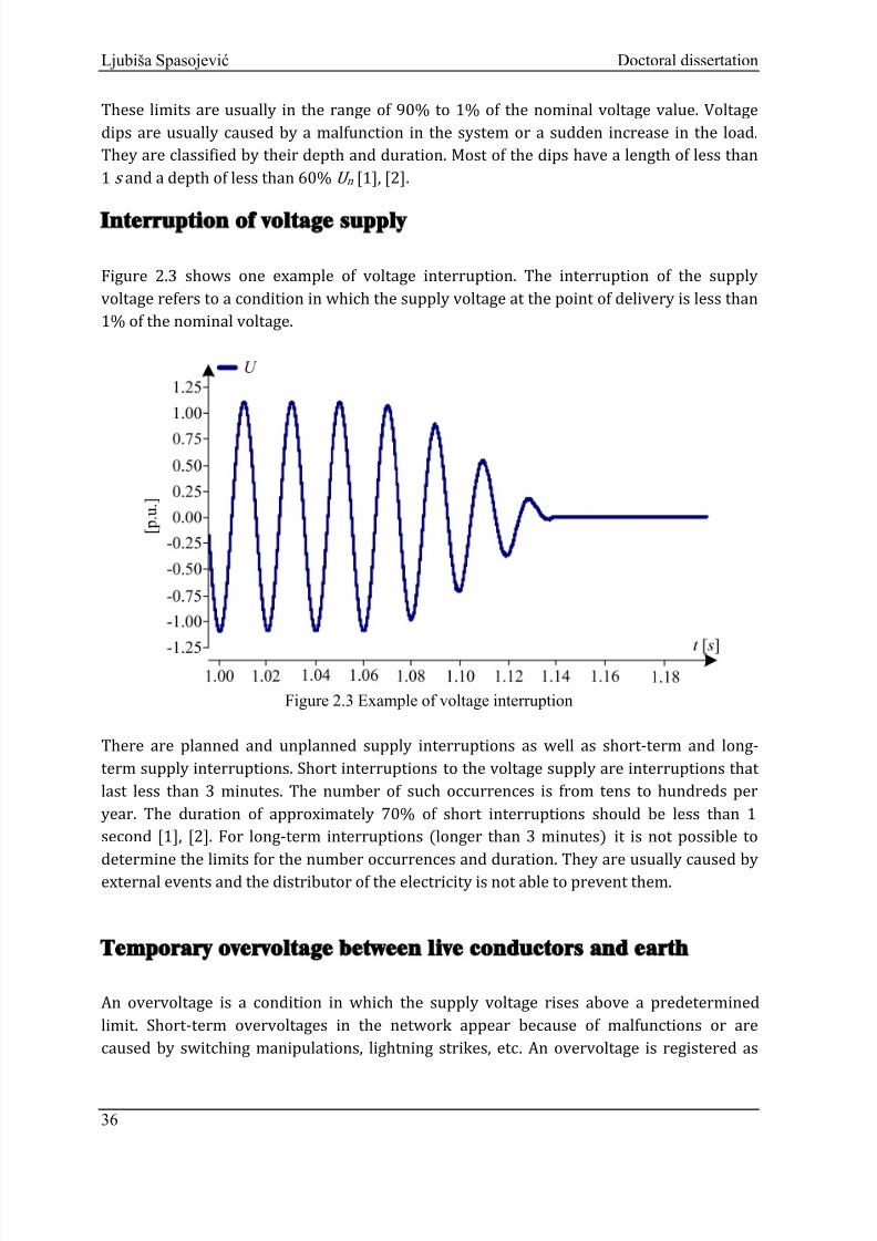
Figure 2.3 shows one example of voltage interruption. The interruption of the supply
voltage refers to a condition in which the supply voltage at the point of delivery is less than1% of the nominal voltage.
Figure 2.3 Example of voltage interruption
There are planned and unplanned supply interruptions as well as short-term and long-term supply interruptions. Short interruptions to the voltage supply are interruptions thatlast less than 3 minutes. The number of such occurrences is from tens to hundreds per
year. The d
uration of approximately 70% of short interruptions should be less than 1second [1], [2]. For long-term interruptions (longer than 3 minutes) it is not possible todetermine the limits for the number occurrences and duration. They are usually caused by
external events and the distributor of the electricity is not able to prevent them.
Temporary overvoltage between live conductors and earth
An overvoltage is a condition in which the supply voltage rises above a predetermined
limit. Short-term overvoltages in the network appear because of malfunctions or are
caused by switching manipulations, lightning strikes, etc. An overvoltage is registered as
36

8/12/2019 Voltage fluctuation in industrial network and compensation measures
http://slidepdf.com/reader/full/voltage-fluctuation-in-industrial-network-and-compensation-measures 43/156
Ljubiša Spasojević Doctoral dissertation
soon as the values of the voltage supply exceeding the limit of +10% U n . Figure 2.4 shows
an example of an overvoltage [1], [2].
Figure 2.4 Example of an overvoltage
Transient overvoltage between live conductors and earth
Figure 2.5 shows a couple of examples of a transient overvoltage.
Figure 2.5 Example of a transient overvoltage
37

8/12/2019 Voltage fluctuation in industrial network and compensation measures
http://slidepdf.com/reader/full/voltage-fluctuation-in-industrial-network-and-compensation-measures 44/156
8/12/2019 Voltage fluctuation in industrial network and compensation measures
http://slidepdf.com/reader/full/voltage-fluctuation-in-industrial-network-and-compensation-measures 45/156
Ljubiša Spasojević Doctoral dissertation
In the standards SIST EN 50160 a voltage unbalance is defined as a period of one week
where under normal operating conditions 95% of the 10 min mean RMS values of thenegative phase sequence component of the supply voltage shall be within the range 0% to
2% of the positive phase sequence component
[1], [2].
Rapid voltage fluctuations
Voltage fluctuations can be described as repetitive or random variations of the voltage
envelope due to sudden changes in the real and reactive power drawn by a load. Thefluctuating loads in the electrical power system, e.g., welding machines and arc furnaces,are the main sources of these voltage fluctuations. The characteristics of voltage
fluctuations depend on the load type and size
, and the power system
’s capacity. The voltage
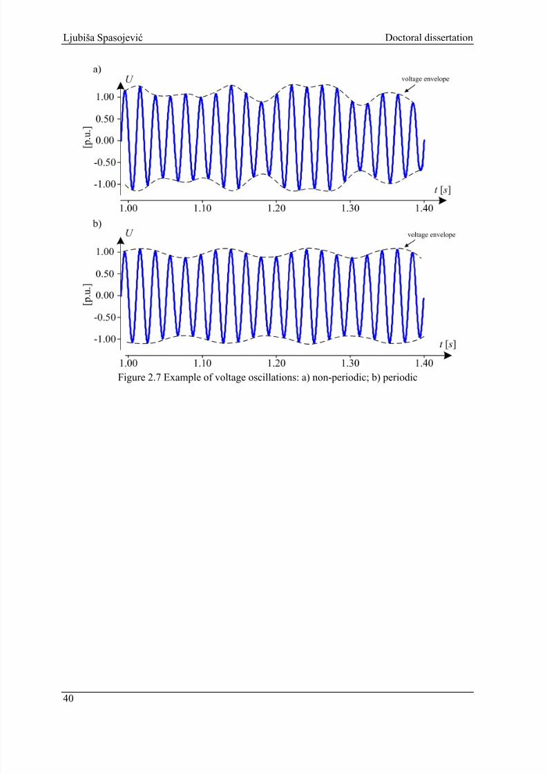
waveform exhibits variations in magnitude due to the fluctuating nature or intermittentoperation of the connected loads. The frequency of the voltage envelope is often referred toas the flicker frequency. Thus, there are two important parameters with respect to thevoltage fluctuations, the frequency of the fluctuation and the magnitude of the fluctuation[1], [2]. Both of these components are significant in the adverse effects of voltagefluctuations. These two parameters can be constants, and in this case there are periodicvoltage oscillations in the network, Figure 2.7a. Also, these parameters can be variable, and
in this case there are non-periodic voltage oscillations in the network, Figure 2.7b.
Most electrical and electronic equipment is designed to operate properly and within the
specifications if the voltage supply varies within ±10% of the nominal value [1], [2]. However, some sensitive devices require a stable incoming voltage for them to performaccurately, such as computers, medical equipment, telecommunications and testequipment. Voltage fluctuations are usually evident in nuisance variations of the lightoutput from incandescent and discharge lighting sources. This is commonly known asflicker, which is a subjective visual impression of the unsteadiness of a light’s flux, whoseluminance fluctuates with time [1], [2].
39
8/12/2019 Voltage fluctuation in industrial network and compensation measures
http://slidepdf.com/reader/full/voltage-fluctuation-in-industrial-network-and-compensation-measures 46/156
Ljubiša Spasojević Doctoral dissertation
Figure 2.7 Example of voltage oscillations: a) non-periodic; b) periodic
40

8/12/2019 Voltage fluctuation in industrial network and compensation measures
http://slidepdf.com/reader/full/voltage-fluctuation-in-industrial-network-and-compensation-measures 47/156
Ljubiša Spasojević Doctoral dissertation
3 Flicker
Voltage fluctuations in power systems can cause a number of harmful technical effects,resulting in a
disruption to production processes and substantial costs. But flicker, with itsnegative physiological results, can affect worker safety as well as productivity. Voltageflicker is a problem that has existed in the power industry for many years. Flicker is defined
as the impression of unsteadiness of the visual sensation induced by a light stimulus whose
luminance or spectral distribution fluctuates with time [3]. In other words, flicker is
defined as the unpleasant sensation experienced by a person when are subjected tochanges that occur in the intensity of the illumination of light sources. These illuminationvariations appear as a consequence of voltage fluctuations, so that a clear relationship canbe established between these disturbances (flicker and voltage fluctuations). This is reasonwhy flicker directly correlates with an
evaluation of voltage quality.
As already mentioned, humans can be sensitive to the light flicker caused by voltagefluctuations. Generally speaking, flicker can significantly impair our vision and causegeneral discomfort and fatigue. Also, flicker affects our vision process and brain reaction,almost always producing discomfort and deterioration in work quality. In some situations,it can even result in workplace accidents because it affects the ergonomics of the
production environment by causing operator fatigue and reduced concentration levels [4], [5].
Since the beginning of the twentieth century there have been a lot of measurements on theeffects of electric flicker on human vision [4], [6]. These measurements studied the
relationship between the light intensity threshold and the luminance variation frequencyas observed by human beings. The aim was to find the condition in which the observer
cannot see flickering light while the fluctuation with the same amplitude can cause aflickering sensation with a lower variation frequency. Tests were performed on people whowere exposed to different variations of waveform voltage, levels of illumination and typesof lighting. The typical frequency range for flicker that can be noticed by the human eye isfrom 0.5 Hz to 35 Hz with amplitudes that begin from 0.2 % of the amplitude at 50 Hz [5], [6], [7]
.
Figure 3.1 shows the flicker detection threshold, i.e., the minimum required amplitude ofthe voltage oscillation at a particular frequency, in which case 50% of the population is able
to detect the flicker. Figure 3.1 shows the border case of the flicker curve (U -f curve) for
sinusoidal and rectangular modulations of the voltage according to [6], [7]. From the figure
it is clear that the human eye is most sensitive to a flicker frequency of approximately 9 Hz.A relative modulation voltage of 0.25% of the basic voltage amplitude at a frequency of8.8 Hz can cause flicker [3], [6]. The flicker of electric lighting causes discomfort in humans
and is especially dangerous for people with epilepsy
[8], [9].
41

8/12/2019 Voltage fluctuation in industrial network and compensation measures
http://slidepdf.com/reader/full/voltage-fluctuation-in-industrial-network-and-compensation-measures 48/156
Ljubiša Spasojević Doctoral dissertation
Figure 3.1 Flicker detection threshold for signals with sinusoidal and rectangular waveforms
Flicker can be measured with a UIE/IEC flickermeter, which is an instrument designed tomeasure any quantity representative of flicker [5]. There are two major indices used in theevaluation of flicker in power systems, the short-term flicker index, (P st ), and the long-termflicker index, (P lt ). The short-term and long-term flicker indicators, which are the output ofthe UIE/IEC flickermeter, are used to describe the characteristics of flicker. The short-term
flicker indicator P st
is the flicker severity evaluated over a short period (10 minutes is usedin practice). P st 1 is the conventional threshold of irritability [5]. The long-term flickerindicator P lt is the flicker severity evaluated over a long period (two hours is used inpractice) using successive P st values.
3.1 Occurrence of flicker and flicker sources
The basic principle of creating flicker can be simply described with Figure 3.2.
Figure 3.2 Creating flicker from voltage oscillations in a power system
Voltage fluctuations at the high-
voltage level of the power system, from its source (sourceflicker) spread to the rest of the power system. Over the transmission lines andtransformers, these oscillations are transmitted to the low-voltage level of the power
42
8/12/2019 Voltage fluctuation in industrial network and compensation measures
http://slidepdf.com/reader/full/voltage-fluctuation-in-industrial-network-and-compensation-measures 49/156
Ljubiša Spasojević Doctoral dissertation
system. The low-voltage level supplies the light sources (light bulbs, lamps, etc.) whichrespond differently to oscillations in the voltage supply system. In the worst case for thedetermined frequency spectrum, the range oscillation of the amplitude is large enough tocause discomfort in people.
Occurrence of flicker
The voltage signal of a power system with the basic frequency f b , can be written as: () = () sin( 2), (3.1)
where U (t ) is the basic amplitude of the voltage and t is the time. If the basic amplitude of
the voltage is constant (U (t )const ), there is no flicker in the network. As a result of
nonlinear dynamic loads, the quick connection and disconnection of some consumers, the
basic amplitude U (t ) of the voltage can fluctuate with time. However, each switching onand off of consumers in the network , changes in their power, active and/or reactive, causesvoltage fluctuations across the entire network. When the value of the basic amplitude U (t )
is not constant (U (t )≠const ), it can be any variable with time. For example, let us take the
function defined by (3.2) with some random frequency f m (frequency of modulation). The
amplitude that describes the fluctuation of U (t
)is
equal to 20
% of theamplitude of the
basic signal U (factor of modulation m 0.2). () = + sin( 2). (3.2)
The modulation factor m is defined by equation (3.3), Figure 3.3.
=
∆ 2�
. (3.3)
Based on everything mentioned above, equation (3.1) can now be written as
() = [1 + sin(2)] sin(2), (3.4)
or in the general form:
(
)=
[
1 + ,
=sin(
2, + ,)]sin(
2),
(3.5)
43
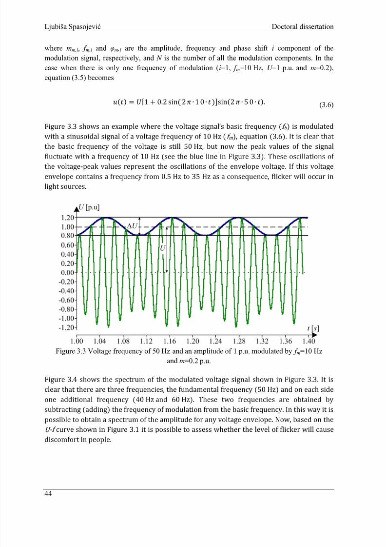
8/12/2019 Voltage fluctuation in industrial network and compensation measures
http://slidepdf.com/reader/full/voltage-fluctuation-in-industrial-network-and-compensation-measures 50/156
Ljubiša Spasojević Doctoral dissertation
where mm,i, f m,i and φm ,i are the amplitude, frequency and phase shift i component of the
modulation signal, respectively, and N is the number of all the modulation components. In the
case when there is only one frequency of modulation (i=1, f m=10 Hz, U =1 p.u. and m=0.2),
equation (3.5) becomes
() = [1 + 0.2 sin( 2 ∙ 1 0 ∙ )]sin(2 ∙ 5 0 ∙ ). (3.6)
Figure 3.3 shows an example where the voltage signal’s basic frequency (f b ) is modulated
with a sinusoidal signal of a voltage frequency of 10 Hz (f m ), equation (3.6). It is clear that
the basic frequency of the voltage is still 50 Hz, but now the peak values of the signal
fluctuate with a frequency of 10 Hz (see the blue line in Figure 3.3). These oscillations of
the voltage-peak values represent the oscillations of the envelope voltage. If this voltage
envelope contains a
frequency from 0.5
Hz to 35 Hz as a
consequence, flicker will occur in
light sources.
Figure 3.3 Voltage frequency of 50 Hz and an amplitude of 1 p.u. modulated by f m=10 Hz
and m=0.2 p.u.
Figure 3.4 shows the spectrum of the modulated voltage signal shown in Figure 3.3. It is
clear that there are three frequencies, the fundamental frequency (50 Hz) and on each sideone additional frequency (40 Hz and 60 Hz). These two frequencies are obtained bysubtracting (adding) the frequency of modulation from the basic frequency. In this way it is
possible to obtain a spectrum of the amplitude for any voltage envelope. Now, based on the
U -f curve shown in Figure 3.1 it is possible to assess whether the level of flicker will cause
discomfort in people.
44

8/12/2019 Voltage fluctuation in industrial network and compensation measures
http://slidepdf.com/reader/full/voltage-fluctuation-in-industrial-network-and-compensation-measures 51/156
Ljubiša Spasojević Doctoral dissertation
Figure 3.4 Amplitude spectrum of the signal from Figure 3.3
The voltage envelope can be calculated in many ways. The first and simplest way is to usethe algorithm of a discrete Fourier transformation (DFT). Using DFT we obtain the
spectrum components of the signal, as shown in Figure 3.4, in the case of the modulated
voltage signal shown in Figure 3.3. The speed of the calculation can be improved with a fast
Fourier transform (FFT), while the accuracy can be improved by using a variable window.Another approach that can be used to calculate the voltage envelope is based on a structure
with a squaring demodulation, as shown in Figure 3.5. Also, this structure is used in the
flickermeter and will be described later.
Figure 3.5 Square modulation structure
As previously mentioned, the main sources of severe voltage fluctuations are industrial
loads with fluctuating power demands.
Also, wind turbines and wave power
, etc.
, can
generate flicker [9], [10].
Arc furnace
An arc furnace is probably the load that produces the most flicker in a power system [9], [10]. When the arc furnace operates, an unstable arc is established between the electrodesand the scrap causing fluctuations of the power consumption and thus a potential flicker
problem. As a rule of thumb, the ratio between the short-circuit capacity at the point of
common coupling (PCC) to the maximum demand of the arc furnace should be greater than80 in order to limit the risk of severe flicker caused by the arc furnace. The best way to
45

8/12/2019 Voltage fluctuation in industrial network and compensation measures
http://slidepdf.com/reader/full/voltage-fluctuation-in-industrial-network-and-compensation-measures 52/156
Ljubiša Spasojević Doctoral dissertation
investigate the actual flicker situation is to perform on-site measurements using a
flickermeter based on [6]. If the arc furnace is connected to a network with changing loadsover time, a good idea is to measure the flicker permanently and thereby observe the trend
of the flicker.
A common method to reduce flicker originating from an arc furnace is to
increase the short-circuit level by installing a new main transformer with ahigher capacity,installing active mitigation equipment like a SVC, etc., or to improve the control strategies
of the arc furnace [11].
Welding machine
Welding machines can also introduce major power-quality problems. A welding machinenormally has a much shorter on-time than off-time, resulting in both current harmonics
and sudden current spikes
, leading to a voltage drop at the point of common coupling. If a
welding machine is a major load on the power network, the current spikes can causesignificant flicker levels if the repetitive frequency is within the flicker frequency window. Wind turbines
The flicker emission from a wind turbine is mainly caused by a fluctuating power
production due to wind-speed changes, since the generated power from a wind turbine is
proportional to the cube of the wind-speed. This means a small change in the wind-speed
will result in a much greater change in the produced output power. If the wind turbine isinstalled in a weak network, the change in output power due to a fluctuating wind speed
can cause considerable voltage changes at the point of common coupling and thereby
flicker. Other reasons for flicker emission originating from a wind turbine are the tower
shadow effect and, for pitch-controlled wind turbines, the limited bandwidth of the pitch
mechanism [12]-[15].
3.2 Estimate of the flicker level
The simplest way to estimate the level of flicker is the use of flicker curves, which are givenin the IEEE standard [6], [7], Figure 3.6. The term “changes per minute” is used as the unitfor the modulating voltage frequency in Figure 3.6. For a modulating voltage, one cycle istwo changes. Thus, 120 changes per minute are equal to 1 Hz. The curves 230 V, 120 V and100 V are obtained from 230 V, 120 V and 100 V, 60 W incandescent-bulb measurements
with a rectangular modulated voltage, respectively. These curves indicate the relativevoltage fluctuation (∆U/U ) with respect to the modulating voltage frequency. The flickercurves shown in
Figure 3.6 give the borderline values of the relative voltage fluctuation for
a corresponding modulating voltage frequency when the short-term flicker indicator (P st )is equal to one. A relative voltage fluctuation below the flicker curve will cause P st to be less
46

8/12/2019 Voltage fluctuation in industrial network and compensation measures
http://slidepdf.com/reader/full/voltage-fluctuation-in-industrial-network-and-compensation-measures 53/156
Ljubiša Spasojević Doctoral dissertation
than one. A relative voltage fluctuation above the flicker curve will cause P st to be higher
than one.
Figure 3.6 Flicker curve for rectangular modulation frequencies presented in IEEE 141-1993,
Pst =1
As the flicker curve is the simplest way to estimate the flicker level, the relative voltagefluctuations for different lamp types to obtain the same flicker level can be compared using
the flicker curves of different lamp types.
Figure 3.7 shows the instantaneous flicker curves
of the four lamp types. Figure 3.7 shows that the incandescent lamp is the most sensitive toflicker, since its modulating voltage amplitudes are the lowest when P inst , max equals one.
Figure 3.7 Instantaneous flicker curves for different lamp types [8]
47

8/12/2019 Voltage fluctuation in industrial network and compensation measures
http://slidepdf.com/reader/full/voltage-fluctuation-in-industrial-network-and-compensation-measures 54/156
Ljubiša Spasojević Doctoral dissertation
The energy-saving lamp is the most insensitive to flicker because of its highest modulating
voltage amplitudes [16]. To obtain the flicker curves of different lamp types, the referenceflicker level needs to be defined. Therefore, the reference values of the relative voltage
fluctuations and the corresponding modulating voltage frequencies, which can cause thereference flicker level, should be defined first. The Standard IEC 61000-4-15 gives thevalues of the sinusoidal modulated voltage for a 230 V incandescent lamp when themaximum instantaneous flicker sensation P inst, max equals one.3.3 Flickermeter
To evaluate the flicker level in power systems, it is necessary to develop a measurement
tool that can represent the relationship between the voltage fluctuations and the human
vision system.
Therefore,a device called a flickermeter has been developed to measure any
quantity representative of flicker. There were four important national flickermeters that
already existed before the flickermeter was defined [6]. The major reason why an
international flickermeter had to be defined was that the national flickermeters did not
give universal results that can indicate the flicker level. All the specifications and all the
necessary provisions of the flickermeter were defined in [6]. In it there is a fundamental
mathematical formulation of the device and the implementation process for testing and
measurement. The specifications of the flickermeter are applicable only to a 60 W,230 V/120 V incandescent lamp. A universal flickermeter model that would cover all types
of lamps does not exist because there is no universal curve of flicker for all lights.
It is important to bear in mind that the primary objective of the flickermeter is not toprovide an evaluation of voltage fluctuations, but of the flicker perception caused by these
fluctuations. To reach to this, the equipment has to be designed so that it is able to
transform the input voltage fluctuations into an output parameter that is proportionally
related to the flicker perception. This is possible by simulating the process of physiologicalvisual perception, which is the so-called lamp-eye-brain chain, [17]. The architecture of the
flickermeter is described in Figure 3.8., which shows the flickermeter can be divided into
two parts, each performing one of the following tasks:
• Simulation of the response of the lamp-eye-brain chain.• Online statistical analysis of the flicker signal and the presentation of results.
The first task is performed by blocks 2, 3 and 4 of Figure 3.8, while the second task isaccomplished by block 5. The response of each block will be analysed in the following
subsections.
48

8/12/2019 Voltage fluctuation in industrial network and compensation measures
http://slidepdf.com/reader/full/voltage-fluctuation-in-industrial-network-and-compensation-measures 55/156
Ljubiša Spasojević Doctoral dissertation
Figure 3.8 Block scheme of flickermeter
Block 1 – input voltage adapter
The supply voltage is the input for this block. In this block there is a voltage-adapting
circuit that can scale the RMS value of the input voltage down to an internal reference level
and does not modify the modulated voltage waveform. This means that all the flicker
measurements can be made independently of the input carrier voltage level. The output of
this block is the normalized RMS value of the input voltage [8].
Block 2 - squaring multiplier
For the referenced incandescent lamp, the light produced by the lamp depends on the
energy consumed by the lamp. The consumed energy by the lamp is proportional to the
square of the input lamp voltage. This block is used to simulate this squaring behaviour ofthe lamp. Since the incandescent lamp has a thermal time constant because of the filamentof the lamp, a low-pass filter function is used to present this time-constant function and it ispart of the weighting filter in block 3 [8]. Let
() = (sin )(1 + sin ), (3.7)
where U(t) is the supply voltage with amplitude A and angular frequency ω , which ismodulated by a sinusoidal waveform with the amplitude m
and angular frequencyω m . The
signal at the output of the squaring multiplier has the following form:
()2 = 22 1 + 22 + 22 1 + 22 sin 2+ 2 28 sin 2( + ) +
2 28 sin 2( ) + 22 sin(2 + ) + 22 sin(2 + ) +
sin + 4 sin 2
(3.8)
49

8/12/2019 Voltage fluctuation in industrial network and compensation measures
http://slidepdf.com/reader/full/voltage-fluctuation-in-industrial-network-and-compensation-measures 56/156
Ljubiša Spasojević Doctoral dissertation
Block 3 – filters
This block consists of series circuits of two filters, i.e., the demodulator filter and the
weighting filter
[8]:
• Demodulator filter (high-pass filter + low-pass filter)
The demodulator filter includes a first-order high-pass filter (3 dB cut-off frequency at0.05 Hz) to filter the DC-component caused by the squaring function in block 2 and a low-
pass filter to filter all the components that are equal to, or greater than, the fundamentalfrequency of the carrier voltage [8]. A sixth-order low-pass Butterworth filter (gives a 3 dBcut-off frequency at 35 Hz for a 50 Hz system and a 3 dB cut-off frequency at 40 Hz for a 60Hz system) is recommended in this block. By filtering the DC component and all the
frequency components higher than the fundamental angular frequencyω, only the
following terms remain: = sin + 4 sin 2. (3.9)
• Weighting filterThe weighting filter simulates the frequency response of a coiled-filament gas-filled lampand the human visual system. As mentioned in block 2, the filament lamp has a thermaltime constant function; it is considered as a low-pass filter with a cut-
off frequency of about
6 Hz. The transfer function of the weighting filter is described as [8]: () =
+ 2 + x1 + 1 + 1 + . (3.10)
For a 60 W 230 V incandescent lamp:
k = 1.74802
λ = 2 π 4.05981 ω1 = 2 π 9.15494
ω2 = 2 π 2.27979
ω3 = 2 π 1.22535
ω4= 2 π 21.9.
For a 60 W 120 V incandescent lamp:
λ = 2 π 4.167375
ω1 = 2 π 9.077169
ω2 = 2 π 2.939902
50
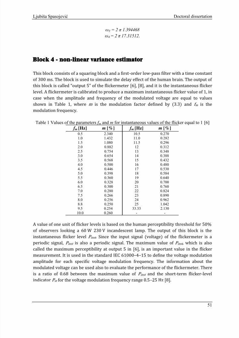
8/12/2019 Voltage fluctuation in industrial network and compensation measures
http://slidepdf.com/reader/full/voltage-fluctuation-in-industrial-network-and-compensation-measures 57/156
Ljubiša Spasojević Doctoral dissertation
ω3 = 2 π 1.394468
ω4 = 2 π 17.31512.
Block 4 - non-linear variance estimator
This block consists of a squaring block and a first-order low-pass filter with a time constantof 300 ms. The block is used to simulate the delay effect of the human brain. The output ofthis block is called “output 5” of the flickermeter [6], [8], and it is the instantaneous flickerlevel. A flickermeter is calibrated to produce a maximum instantaneous flicker value of 1, incase when the amplitude and frequency of the modulated voltage are equal to valuesshown in Table 1, where m is the modulation factor defined by (3.3) and f m is the
modulation frequency.
Table 1 Values of the parameters f m and m for instantaneous values of the flicker equal to 1 [6]
f m [Hz] m [%] f m [Hz] m [%]0.5 2.340 10.5 0.270
1.0 1.432 11.0 0.282
1.5 1.080 11.5 0.296
2.0 0.882 12 0.312
2.5 0.754 13 0.3483.0 0.654 14 0.388
3.5 0.568 15 0.432
4.0 0.500 16 0.480
4.5 0.446 17 0.5305.0 0.398 18 0.584
5.5 0.360 19 0.640
6.0 0.328 20 0.700
6.5 0.300 21 0.760
7.0 0.280 22 0.824
7.5 0.266 23 0.890
8.0 0.256 24 0.962
8.8 0.250 25 1.0429.5 0.254 33.33 2.130
10.0 0.260 - -
A value of one unit of flicker levels is based on the human perceptibility threshold for 50%of observers looking a 60 W 230 V incandescent lamp. The output of this block is theinstantaneous flicker level P inst . Since the input signal (voltage) of the flickermeter is aperiodic signal, P inst is also a periodic signal. The maximum value of P inst , which is alsocalled the maximum perceptibility at output 5 in [6], is an important value in the flicker
measurement. It is used in the standard IEC 61000–4–15 to define the voltage modulationamplitude for each specific voltage modulation frequency. The information about the
modulated voltage can be used also to evaluate the performance of the flickermeter. Thereis a ratio of 0.68 between the maximum value of P inst and the short-term flicker-level
indicator P st
for the voltage modulation frequency range 0.5–
25 Hz
[8].
51

8/12/2019 Voltage fluctuation in industrial network and compensation measures
http://slidepdf.com/reader/full/voltage-fluctuation-in-industrial-network-and-compensation-measures 58/156
Ljubiša Spasojević Doctoral dissertation
Block 5 - statistical calculation block Block 5 is used for the statistical calculation of the short-term flicker indicator P st and the
long-term flicker indicator P lt using the time-at-level method
[6].
• Short-term flicker indicator ( P st)The P st value represents the perceived flicker severity averaged over a ten-minutemeasurement interval. A value of 1.0 or higher represents a flicker level that will bringannoyance to an observer. The P st value can be calculated using the equation:
= 0.0314. + 0.0525 + 0.0657 + 0.28 + 0.08 , (3.11)
where the percentiles P 0.1, P 1, P 3, P 10 and P 50 are the instantaneous flicker levels exceeding0.1 %, 1 %, 3 %, 10 % and 50 % of the time during the observation period. The suffix s inthe equation indicates that the smoothed values should be used, which are shown in theequation below. P 1s , P 3s , P 10s and P 50s can be determined as: P1s = (P0.7 + P1 + P1.3 ) / 3, (3.12)
P3s = (P2.2 + P3 + P4 ) / 3, (3.13)
P10s = (P6 + P8 + P10 + P13 + P17 ) / 5, (3.14)
P50s = (P30 + P50 + P80 ) / 3. (3.15)
The IEC standard gives four observation intervals (1 min, 5 min, 10 min and 15 min).However, only the 10-min interval will be used for the P st assessment during field
measurements. The other three intervals can be used for the laboratory measurements [8]. The 10-min interval was chosen because it is sufficiently short to characterize in detail a
load whose operating cycle is long (e.g., an arc furnace) and also sufficiently long so that itis not affected by very isolated short-term variations.
• Long-term flicker indicator ( Plt)
Since the short-term flicker indicator is only suitable to assess the flicker caused by an
individual source with a short duty-cycle, another flicker indicator, which can assess the52

8/12/2019 Voltage fluctuation in industrial network and compensation measures
http://slidepdf.com/reader/full/voltage-fluctuation-in-industrial-network-and-compensation-measures 59/156
Ljubiša Spasojević Doctoral dissertation
combined effects of several flicker sources (e.g., welders, motors) operating randomly, or
flicker sources having a long and variable duty-cycle, should be defined. The long-term
flicker indicator P lt has been defined for this purpose. It can be derived from the short-term
flicker indictor P st values over a certain measuring period that relates to the duty-cycle of
the flicker sources. The mathematical equation used to calculate P lt is shown below: = ∑ =
. (3.16)
Here, N is the number of the P st measurements during the P lt observation period [8]. Normally, in practice, 2 hours is selected as the observation period for the long-term flicker
indicator P lt . To calculate P lt values, 2 hours must be a discrete time interval. Two-hour
sliding windows are not allowed. Since theP st
observation interval is 10 minutes and theP lt
interval is 2 hours, the number of measurements N will be 12 [8].
53

8/12/2019 Voltage fluctuation in industrial network and compensation measures
http://slidepdf.com/reader/full/voltage-fluctuation-in-industrial-network-and-compensation-measures 60/156
8/12/2019 Voltage fluctuation in industrial network and compensation measures
http://slidepdf.com/reader/full/voltage-fluctuation-in-industrial-network-and-compensation-measures 61/156
Ljubiša Spasojević Doctoral dissertation
4 Electric arc furnace
The use of electric arc furnaces (EAFs) has grown rapidly over the past 30 or so years. The
main reason for this is
their productivity, precision, flexibility and some advancedapplications for steelmaking. Of all the steel made today, 36% is produced by the electric-
arc-furnace route and this share will increase to 50% by 2030 [16]-[18]. On the other hand,their time-varying nature and non-linear voltage-current characteristics have a large, negative influence on the power quality. They are major sources of voltage oscillations inpower system that can produce the effect known as flicker. Also, EAFs need a significantquantity of reactive power, which may give rise to the voltage instability in a power system
without proper compensation [16]-[18].
Anelectric arc furnace converts electrical energy to thermal energy in the form of an
electric arc in order to melt the raw materials held by the furnace. The arc is establishedbetween the electrode and the melting bath and is characterized by a low voltage and a
high current. Electric arc furnaces are used for smelting and refining metals, mainly the
iron in the steel production. Using an electric arc we can achieve an extremely high
temperature and a high power density. Due to the high concentration of power in a smallarea, an equal allocation of heat is not possible [16]-[18]. Therefore, electric arc are used
for melting metals and alloys, while for heat treatments they are inappropriate.
Electric arc furnacesbased on alternating current (
AC) and direct current (
DC) represent
one of the most intensive, disturbing loads in sub-transmission or transmission electricpower systems. They are characterized by rapid changes in the absorbed powers, especially during the initial stage of melting. Nowadays, arc furnaces are designed for very
large power-input ratings and due to the nature of both the electrical arc and the melt-down process, these devices can cause large power-quality problems on the electricity net,mainly harmonics, inter-harmonics, flicker and voltage imbalances. The Voltage-Current(U -I ) characteristic of the arc is non-linear, which can cause harmonic currents [18], [19]. In general, electric arc furnaces are classified according to their method of heating, as
follows
:
• furnace with a direct electrical arc
• furnace with an indirect electrical arc
• furnace with a submerged arc [19] - [21].
4.1 Furnace with a direct electrical arc
For these furnaces there is a
specific low voltage,a high current and the electric arc is
established between graphite electrodes and batches that gradually heat up and melt.Direct arc electric furnaces are very popular for the melting of alloy steels and range in size55

8/12/2019 Voltage fluctuation in industrial network and compensation measures
http://slidepdf.com/reader/full/voltage-fluctuation-in-industrial-network-and-compensation-measures 62/156
Ljubiša Spasojević Doctoral dissertation
from a few kilograms, for laboratory units, to in excess of 100 tonnes per batch. Typically,the units found in foundries are in the range of 1 to 10 tonnes [19] - [21].
The scheme of an
EAF with a direct electrical arc is presented in
Figure 4.1. The furnace
consists of a spherical hearth (bottom), a cylindrical shell and a swinging water-cooleddome-shaped roof. The roof has three holes for consumable graphite electrodes held by a
clamping mechanism. The mechanism provides for the independent lifting and lowering of
each electrode. The water-cooled electrode holders also serve as contacts for transmitting
the electric current supplied by water-cooled cables (tubes). The electrode and the scrapform the star connection of three-phase current, in which the scrap is the common junction.The furnace is mounted on a tilting mechanism for tapping the molten steel through a tap
hole with a pour spout located on the rear side of the shell. The charge door, through whichthe slag components and alloying additives are charged, is located on the front side of thefurnace shell. The charge door is also used for removing the slag (de-slagging). The scrap is
commonly charged from the furnace top. The roof with the electrodes is swung aside before the
scrap charging. The scrap arranged in the charge basket is transferred to the furnace by a crane
and then dropped into the shell [19], [20].
Figure 4.1 Furnace with a direct electrical arc
Advantage of a direct arc furnace: • Quicker readiness for use
• Longer hearth life
• Ease of repair
• Great independence of the quality of the charge
• Analysis of the metal can be kept to an accurate limit.
The major disadvantage of this typeof furnace is the high cost of the electricity and the cost
of the equipment. The heating costs are higher than for other furnaces [19] - [21]. This,
Slag Arc
Spout
Charging
door
Molten steel
Electrodes
56

8/12/2019 Voltage fluctuation in industrial network and compensation measures
http://slidepdf.com/reader/full/voltage-fluctuation-in-industrial-network-and-compensation-measures 63/156
Ljubiša Spasojević Doctoral dissertation
however, can be adjusted, to some extent , by using low-cost scrap turning or boring as the
metal charge.
4.2 Indirect arc furnaces
Generally, indirect arc furnaces consist of a horizontal barrel shape steel shell lined with
refractories. The melting is effected by the arcing between two horizontally opposed
carbon electrodes or graphite electrodes. The heating is via radiation from the arc to the
charge. The barrel-shaped shell is designed to rotate and reverse through approximately180° C in order to avoid excessive heating of the refractories above the melt level and to
increase the melting efficiency of the unit. The furnace is mounted on the rollers and the
rollers can be driven to rock the furnace. The metal melts because of the heat radiated from
the arc and the heat from the hot refractory lining. Indirect arc furnaces are suitable for
melting a wide range of alloys
, but are particularly popular for the production of copper
base alloys. The units operate on a single-phase power supply and hence the size is usually
limited to relatively small units. The scheme of an EAF with an indirect electrical arc is
presented in Figure 4.2 [19], [20].
Figure 4.2 Furnace with an indirect electrical arc
4.3 Furnace with a submerged arc
A submerged arc furnace is mainly used for ferroalloy production, e.g., ferromanganese,ferronickel, ferrosilicon, ferrochrome, silicon manganese. In furnaces with a submerged arc
the electrodes are directly put into the molten alloy. The electric arcs are established in the
gaseous area within the slag. The charge is heated by the heat emitted in the arcs and also
by the Joule heat developed as the current passes through the charge. The energy
consumption of these furnaces is relatively high, and for high-carbon ferrochrome the
57

8/12/2019 Voltage fluctuation in industrial network and compensation measures
http://slidepdf.com/reader/full/voltage-fluctuation-in-industrial-network-and-compensation-measures 64/156
Ljubiša Spasojević Doctoral dissertation
electrical energy consumption varies between 2000 kWh/T alloy, with pre-reduction to4000 kWh/T alloy, without pre-reduction and feed preheating [20]. These furnaces
represent the most powerful consumers of electricity. Figure 4.3 shows the scheme of the
submerged arc furnace.
Figure 4.3 Furnace with a submerged arc
4.4 Electric arc
An electric arc is the electrical breakdown of a gas that produces an on-going plasmadischarge, resulting from a current through normally non-conductive media such as air.The electric arc was first described in 1802 as a "special fluid with electrical properties", byVasily V. Petrov, a Russian scientist [21].
The arc occurs in the gas-filled space between at least two conductive electrodes that are
made of tungsten or carbon, and it results in a very high temperature. The electric arc is a
continuous discharge and may occur either in direct-current circuits or in alternating
circuits, while a similar electric spark discharge is momentary. Under the influence of an
electric field the particles between the electrodes are electrified and their movement is
directed. Positively charged particles are directed towards the cathode, while negativelycharged particles move towards the anode. The electric arc has a non-linear relationship
between the current and the voltage characterized by a small cathode voltage drop (from10 to 20 V) and high current density (from 100 A/cm2 to over 1000 A/cm2). The current
level between the electrodes is directly proportional to the gradient of the electric
potential. Figure 4.4 shows the voltage-current (U -I ) characteristics of the electric arc.
Normally, gas is an electrical insulator
[19], [20].
58

8/12/2019 Voltage fluctuation in industrial network and compensation measures
http://slidepdf.com/reader/full/voltage-fluctuation-in-industrial-network-and-compensation-measures 65/156
Ljubiša Spasojević Doctoral dissertation
With a small voltage difference between the electrodes a small current (negligible) that is
proportional to the voltage will flow. This can be explained by the higher speed of the free
electrons and the positive ions in the stronger electric field, Figure 4.4 point 1. Increasing
the voltage at point
2 does not cause an increased current. This can be explained by the
limited number of charge carriers. If the voltage level rises above point 2, the electronsaccelerated at that level cause the ionization of other molecules. In this way the number of
charge carriers is increased and the current begins to increase with increasing voltage [19], [20], [21].
Figure 4.4 Voltage-current characteristic of an electric arc
The voltage at point 3 is characteristic for a given gas environment and the type ofelectrodes. Under the influence of this voltage, the secondary ionization of space occurs,which is manifested in the form of sparks. The quantity of the charge carrier has increased
to such an extent that the environment can be treated as being conductive. The voltage
between the electrodes is decreased and this generates the negative U -I characteristic of
the arc. At point 4, the arc is established; electrons with a high speed collide with theneutral atoms (molecules) and ionize them [20], [21].
Electric arc of direct current
An electrical arc of a direct current is obtained with the short circuit of two graphite
electrodes connected to a source of direct-current voltage. Following a brief short circuitthe electrodes move apart and between them the arc is established, Figure 4.5. Positively
charged particles move to the cathode, become neutral and accumulate on it. That is the
reason why the top of the cathode is a conical surface, while at the anode crater is formed.Electric arc that burns between the electrodes has a surface temperature of over 4000ºCand is characterized by a different electrode voltage drop. The anode
’s voltage drop is
59
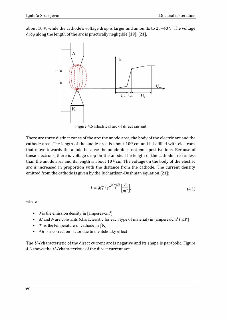
8/12/2019 Voltage fluctuation in industrial network and compensation measures
http://slidepdf.com/reader/full/voltage-fluctuation-in-industrial-network-and-compensation-measures 66/156
Ljubiša Spasojević Doctoral dissertation
about 10 V, while the cathode's voltage drop is larger and amounts to 25–40 V. The voltage
drop along the length of the arc is practically negligible [19], [21].
Figure 4.5 Electrical arc of direct current
There are three distinct zones of the arc: the anode area, the body of the electric arc and the
cathode area. The length of the anode area is about 10-3 cm and it is filled with electrons
that move towards the anode because the anode does not emit positive ions. Because ofthese electrons, there is voltage drop on
the anode. The length of the cathode area is less
than the anode area and its length is about 10-5 cm. The voltage on the body of the electricarc is increased in proportion with the distance from the cathode. The current density
emitted from the cathode is given by the Richardson-Dushman equation [21]: = −−∆ , (4.1)
where:
•
J is the emission density in [amperes/cm
2
]• M and N are constants (characteristic for each type of material) in [amperes/cm2 (ºK)2]
• T is the temperature of cathode in [ºK]
• ∆ B is a correction factor due to the Schottky effect
The U -I characteristic of the direct current arc is negative and its shape is parabolic. Figure4.6 shows the U -I characteristic of the direct current arc.
lArc
Uarc
A
K
Uk Uk Ua
60

8/12/2019 Voltage fluctuation in industrial network and compensation measures
http://slidepdf.com/reader/full/voltage-fluctuation-in-industrial-network-and-compensation-measures 67/156
Ljubiša Spasojević Doctoral dissertation
Figure 4.6 Static characteristic of a DC electric arc
Changing the arc length (l ), i.e., the distance between the electrodes, means the shape of thecurve is changed. Also, the voltage level that is necessary for the electric arc is modified.
Increasing the current of the arc as result , there is an increase of the temperature into the
electric arc. The temperature of the electric arc directly influences the ionisation, i.e., ahigher temperature means better ionisation (higher conductance of arc). Based on theresults of much experimental research, the equations that describe the characteristic
values and lengths of the electric arc have been formulated [19]. Equation (4.2) describes
the characteristic values of the electric arc.
= + + + , (4.2)
where:
• U arc is the voltage of the arc [V]
• I arc is the current of the arc [A]
• l is the length of the arc [m]
• A, B, C, D are constants that depend on the type electrodes and the gas environment.
Based on the results of many experimental measurements, a simplified equation that
describes the length of the arc can be written as: = +40, (4.3)
where:
• U arc is the voltage of the arc [V]
•
E arc is the electric field in the arc (approximately constant 1700-1900 V/m)• 40 is a constant that represents the drop voltage on the electrodes.
61

8/12/2019 Voltage fluctuation in industrial network and compensation measures
http://slidepdf.com/reader/full/voltage-fluctuation-in-industrial-network-and-compensation-measures 68/156
Ljubiša Spasojević Doctoral dissertation
Electric arc of alternating current
In case when the voltage supply is alternating, the conditions of the arc burning and its
characteristics are very different. The forms of the U -I characteristic of the electrical arc
depend on the conditions of burning of the arc, essentially from its cooling conditions. Thedynamic characteristics of a low-power electric arc for the conditions of intensive cooling
are shown in Figure 4.7.
Figure 4.7 Dynamic characteristics of the arc
During each pass of the current through zero, the area is cooled and deionized.Furthermore, the resistance of the space between the electrodes is increased and there is
demand for a higher voltage level for the establish arc (voltage peak). This voltage peak
represents the voltage level of the arc ignition. With the advent current of the arc, thevoltage of arc is dropped to minimum for maximum value of current. The decreasing
current causes the voltage to increase to the point when the arc disappears (the voltagelevel of shutdown). In the case when the power of the arc is higher and the conditions of
the cooling are
lower, the voltage peaks andthe voltage level of the shutdown are lower.
The dynamic characteristics of a high-power electric arc for low conditions of cooling areshown in Figure 4.8.
62

8/12/2019 Voltage fluctuation in industrial network and compensation measures
http://slidepdf.com/reader/full/voltage-fluctuation-in-industrial-network-and-compensation-measures 69/156
Ljubiša Spasojević Doctoral dissertation
Figure 4.8 Dynamic characteristics of a high-power electric arc
This form of the U -I features is characteristic for high-power electric arc furnaces for
melting steel, were the arc burns almost constantly. For the values of the arc current equalto 10-15 kA, the measured current density in the AC electric arc is approximately 10 7 A/m2,while the diameter of the arc is about 2 cm. For larger values of the arc current, the current
range is 100 kA, the current density is 108 A/m2 and the diameter of the arc is about 3 cm.The major useful characteristic of the arc is its high density heat, which can reach a value of
2
GW/m2. The temperatures on the surface of the arc are in the
range 4000–
5000º
C, whilethe temperature in its interior can reach 15000º
C [19], [20].
63

8/12/2019 Voltage fluctuation in industrial network and compensation measures
http://slidepdf.com/reader/full/voltage-fluctuation-in-industrial-network-and-compensation-measures 70/156
8/12/2019 Voltage fluctuation in industrial network and compensation measures
http://slidepdf.com/reader/full/voltage-fluctuation-in-industrial-network-and-compensation-measures 71/156
Ljubiša Spasojević Doctoral dissertation
5 Dynamic reactive-power compensation
The lack of static compensation means an inability to control the power factor in conditions
of variable load. In the dynamic type of reactive-power compensation the reactive power is
produced in a way that there is the possibility to quickly change the production level, regardless of the voltage level at the connection point. Dynamic reactive-powercompensation can be stepped or continuous, depending on the configuration of the static
compensators. Therefore, dynamic sources can increase (or decrease) the level of reactive
power in the conditions of the voltage drop (overvoltage) and thus avoid a voltage collapse.Some of the major advantages of the use of dynamic reactive-power compensation are: • compensation of the reactive power, which requires consumers with rapid changes in the
load
•
fast switching on and off of the capacitor, without a time delay for the discharge of acapacitor
• no transient phenomena
• extending the lifetime of the system to compensate
Static compensators based on power-electronic, synchronous generators and
compensators represent the dynamic sources of reactive power.
5.1 Flexible alternating-current transmission system
The technological advancement of power-electronics has enabled the production of more
modern compensating devices and devices for the management of more complex power
systems. The Flexible Alternating Current Transmission System (FACTS) is a concept basedon power-electronics that enhance the value of transmission networks by increasing the
use of their capacity [22]. FACTS technology has created new opportunities for powermanagement and achieving the full capacity of transmission networks. The idea for the
development of these devices was born in the
1980sin order to solve problems around the
construction of transmission lines and facilitate the control of transmission power [23], [24]. However, as already mentioned, the main reasons were the increase of the maximum
transmission capacity of the existing transmission system and the management of power
flows on certain routes.
FACTS devices work by acting on certain parameters, such as serial or parallel impedance,current, voltage, phase angle, etc [24]. Using these devices is particularly justified inapplications that demand one or more of the following characteristics: •
fast dynamic response• ability for frequent changes of output values
65
8/12/2019 Voltage fluctuation in industrial network and compensation measures
http://slidepdf.com/reader/full/voltage-fluctuation-in-industrial-network-and-compensation-measures 72/156
Ljubiša Spasojević Doctoral dissertation
• finely adjustable output values
• rapid implementation in order to achieve a significant increase in capacity
• reduction of transmission costs.
FACTS technology is not just a device that solves a certain problem, it is more of a set ofdevices that can be applied individually or in coordination with other devices in order to
manage one or more parameters of the system [24]. In general, FACTS devices, depending
on the connection to the transmission system, could be divided as follows: • serial devices
• parallel devices
• combined serial-serial devices
• combined serial-parallel devices.
Serial FACTS devices are very effective in the management of power flow as well asincreasing the stability of the system. Using a serial compensator the total effective series
impedance between two points of the transmission line can be reduced by influencing the
flow of active power. The possibility of controlling the power flow can be used to increase
the limit of the transient stability and the damping of the power oscillation [22], [24]. FACTS devices for series compensation are composed of capacitors, reactors and thyristorconverters. Types of serial FACTS devices are [24]:
• Static Synchronous Series Capacitor – SSSC
• Thyristor Controlled Series Capacitor – TCSC
• Thyristor Controlled Series Reactor – TCSR
• Thyristor Switched Series Reactor – TSSR
• Thyristor Switched Series Capacitor – TSSC.
Parallel compensation is used to influence the electrical characteristics of the transmission
lines in order to increase the initial value of the power that can be transmitted through a
transmission line and control the voltage values along the transmission line [24]. Parallel
FACTS devices
are:
• Static Synchronous Generator – SSG
• Static Synchronous Compensator – STATCOM
• Static Var Compensator – SVC
• Battery energy storage system – BESS.
Combined FACTS devices are composed of mutual combination serial and parallel devices.Someone of most important FACTS devices of this type are:
66
8/12/2019 Voltage fluctuation in industrial network and compensation measures
http://slidepdf.com/reader/full/voltage-fluctuation-in-industrial-network-and-compensation-measures 73/156
Ljubiša Spasojević Doctoral dissertation
• Unified Power Flow Controller – UPFC
• Thyristor-controlled phase-shifting transformers – TCPST
• Interline Power Flow Controller (IPFC).
5.2 Static VAr Compensator
Static VAr compensator (SVC) is the common name for several types of FACTS devices. SVC
is a parallel connected static VAr generator or absorber whose output is adjusted toexchange the capacitive or inductive current in order to achieve the control of specific
parameters of the power system (typically the voltage on the BUS). With the application ofSVC, the power-transmission capability of the electric network can be increased, the
system voltage can be stabilized,the low-
frequency oscillation of system can be damped,and sub-synchronous oscillation can be suppressed, while the application of SVC in powerdistribution network, voltage fluctuation, flicker, negative sequence and harmonicinterference caused by nonlinear loads and impact loads can be reduced, the power qualitycan be improved, the productivity and power factor can be increased, the reactive tide canbe decreased, and the net loss can be reduced. These types of devices are mainly controlled
by a thyristor and the most important of these are thyristor-controlled reactors (TCRs) and
thyristor-Switched capacitors (TSCs). The structure of the SVC is the obtained combinationof TCR and TSC, such as the Fixed Capacitor Thyristor Controlled Reactor (FC-TCR)structure and the Thyristor Swit ched Capacitor Thyristor Controlled Reactor (SC-TCR)
structure. This combination is ensures greater flexibility in the realization of control work
and reducing the injection harmonics of the current.
FC-TCR structure
The TCR structure can ensure continuously controllable reactive power only in the lagging
power-factor range. In order to achieve dynamic, controllable, reactive power also on the
leading power-
factor domain, a fixed-capacitor
(FC) structureis connected in parallel. The
FC-TCR compensator consists of a fixed capacitor bank utilized as high-order currentharmonics filters, and parallel reactors whose fundamental current harmonic is controlledby means of thyristor AC switches [24]. The FC-TCR structure can be seen in Figure 5.1. This type of SVC can provide an adjustment of the reactive power in bothquadrants, i.e., capacitive and inductive. The capacitors ensure the constant capacitivereactive power (current, I FC ) for the devices and usually inductance (L ) is added in series, Figure 5.1, which forms a resonant circuit that filters harmonic and/or interharmonic fromthe network [24]. The variable inductive reactive power (current, I TCR ) is ensured by thethyristor-controlled reactors. The sum of the capacitive and inductive reactive powers
represents the total reactive power (current,I SVC
), equation (
5.
1), which the device
generates or absorbs over the range from –I FC to –I TCR +I FC .
67

8/12/2019 Voltage fluctuation in industrial network and compensation measures
http://slidepdf.com/reader/full/voltage-fluctuation-in-industrial-network-and-compensation-measures 74/156
Ljubiša Spasojević Doctoral dissertation
= + (5.1)
Figure 5.1 FC-TCR structure of SVC
The voltage-current characteristic for the FC-TCR is shown in Figure 5.2. The compensator voltage-current characteristic encompasses the area ofinductive and capacitive loadings within the boundaries determined by the FC and thethyristor-controlled reactor powers. It should be emphasized that the compensator is a
source of odd harmonics and, if the control angles of antiparallel-connected thyristors areunequal, even harmonics can occur too. The third harmonics in the compensator currentcan be cancelled by the delta connection of the reactor branches.
68
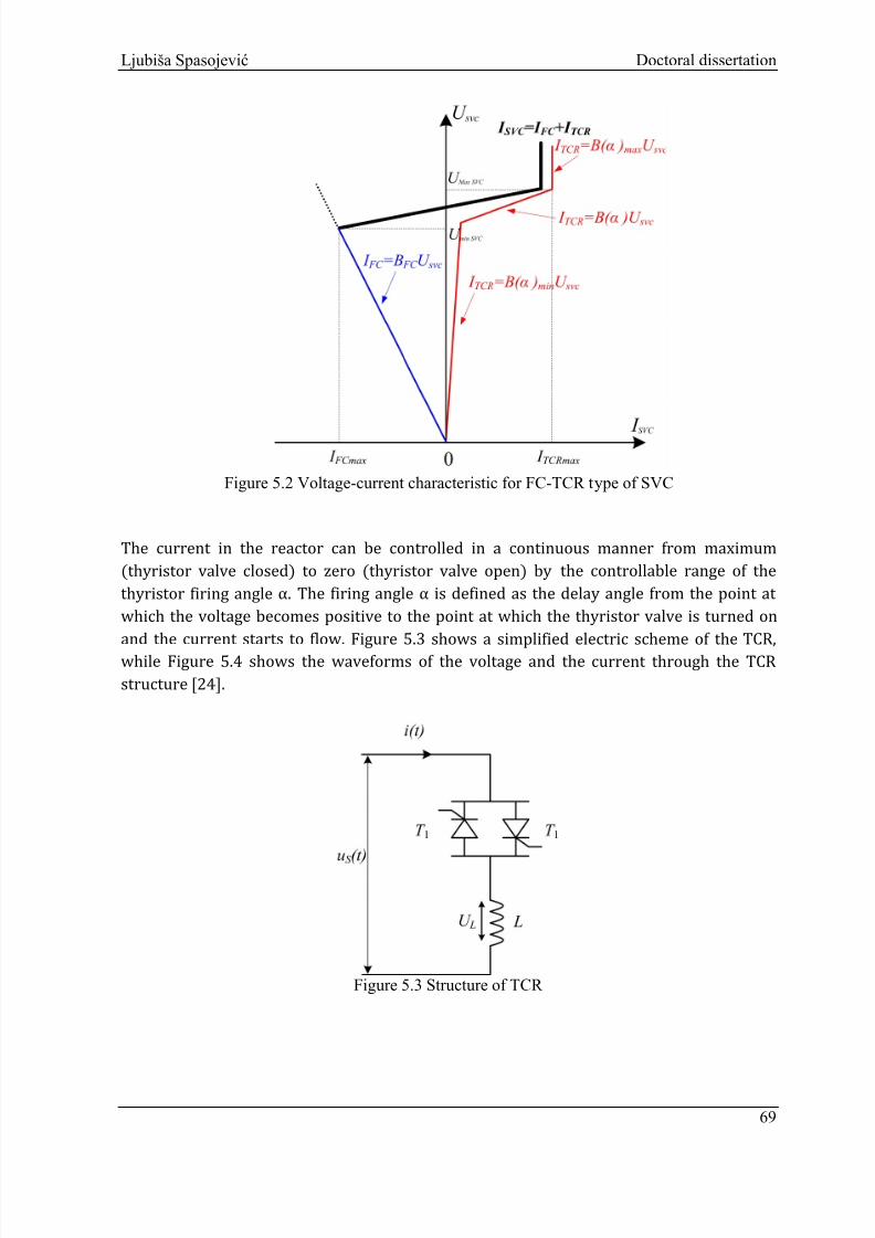
8/12/2019 Voltage fluctuation in industrial network and compensation measures
http://slidepdf.com/reader/full/voltage-fluctuation-in-industrial-network-and-compensation-measures 75/156
Ljubiša Spasojević Doctoral dissertation
Figure 5.2 Voltage-current characteristic for FC-TCR type of SVC
The current in the reactor can be controlled in a continuous manner from maximum(thyristor valve closed) to zero (thyristor valve open) by the controllable range of the
thyristor firing angle α. The firing angle
α is defined as the delay angle from the point at
which the voltage becomes positive to the point at which the thyristor valve is turned onand the current starts to flow. Figure 5.3 shows a simplified electric scheme of the TCR,while Figure 5.4 shows the waveforms of the voltage and the current through the TCRstructure [24].
Figure 5.3 Structure of TCR
69

8/12/2019 Voltage fluctuation in industrial network and compensation measures
http://slidepdf.com/reader/full/voltage-fluctuation-in-industrial-network-and-compensation-measures 76/156
Ljubiša Spasojević Doctoral dissertation
Figure 5.4 Waveforms of voltage and current through the TCR structure
Let us define the source voltage as:
() = sin , (5.2)
where U S is the peak value of the applied voltage and ω is the angular frequency of the
supply voltage [24].
The current through the inductance L is obtained with:
(
) (
)=
0, (5.3)
() =1 () + . (5.4)
For the boundary condition i(ωt=α)=0,
() = (cos + cos ). (5.5)
Using Fourier analyses we can derive an expression for the fundamental reactor current asa function of angle α, equation (5.6) [24].
() = (1 2 1 sin 2), (5.6)
where U is the amplitude of the applied ac voltage, L is the inductance of the thyristor-controlled reactor, and ω is the angular frequency of the applied voltage. Equation (5.6) can be rewritten as:
70

8/12/2019 Voltage fluctuation in industrial network and compensation measures
http://slidepdf.com/reader/full/voltage-fluctuation-in-industrial-network-and-compensation-measures 77/156
Ljubiša Spasojević Doctoral dissertation
() = (), (5.7)
where B TCR represents the reactive admittance (susceptance) of the TCR defined as: () = (1 2 1 sin 2), (5.8)
=1. (5.9)
The variation of the per–unit value of B TCR with the firing angle α is shown in
Figure 5.5. The per–unit value of B TCR is obtained with respect to its maximum value B max as
the base quantity
[24].
Figure 5.5 Control characteristics of the TCR susceptance, BTCR (α)
71

8/12/2019 Voltage fluctuation in industrial network and compensation measures
http://slidepdf.com/reader/full/voltage-fluctuation-in-industrial-network-and-compensation-measures 78/156

8/12/2019 Voltage fluctuation in industrial network and compensation measures
http://slidepdf.com/reader/full/voltage-fluctuation-in-industrial-network-and-compensation-measures 79/156
Ljubiša Spasojević Doctoral dissertation
6 The Modelling of Electric Arc Furnaces
One of the main sources of voltage fluctuations in power systems are electric arc furnaces.
It is therefore important to develop accurate models of the electric arc furnace for network
power-quality analyses that make it possible to simulate the conditions that cause flicker.There are various methods for modelling electric arc furnaces. All these models can beclassified into four groups:• Time-domain analysis methods [25], [26], [27],
• Frequency-domain analysis methods [28], [29],
• Chaotic variation methods [30], [31],
• Models based on the electric arc furnace’s periodic draw of active and reactive power[32].
Usually, the electric arc furnace (the electric arc) is modelled as a voltage source. Theamplitudes of the frequency components of the voltage source are time-modulated to
describe the arc-length variations that cause network-voltage fluctuations. Determining thefrequency characteristic of the arc length can be a difficult task. To simulate the arc -lengthvariation, a stochastic or a deterministic approach can be used. The stochastic approachprovides random variations of the length, which is closer to reality, but makes themathematical analysis complex and requires longer simulation times due to the need for astatistical evaluation. With the deterministic approach the arc length varies as a sine
function with a selected frequency. However, this approach does not fully describe theoperation of the electric arc furnace, but allows a much easier simulation with shortersimulation times and without any additional statistical assessment of the results. The
deterministic model usually provides higher flicker levels at a certain operating point of the
electric arc furnace compared to the stochastic model. However, deterministic modelling isnot entirely satisfactory, because a nonlinear phenomenon is modelled as a linear one. In [26] the arc length is modelled as a controlled voltage source based on a nonlinear u-i
characteristic. The time modulation of the voltage source is achieved by two different time-
variation laws based on sinusoidal and white-noise functions. In the first case (sinusoidal
law) a frequency of 8.8 Hz for the changing arc length is chosen, as this is the frequencythat lies at the centre of perceptivity of the flicker. This modelling approach, when only theworst frequency is considered, ignores the whole spectrum of characteristic flickerfrequencies that can have a significant effect on the flicker level. A more realistic modellingof the furnace operation can be achieved with the addition of a white-noise, time modulation of the arc length, as in [26] and also in [33]. However, neither author explains
or mentions how to specify the white-noise function that would be able to accuratelydescribe the spectrum of characteristic flicker frequencies. An alternative approach to modelling the arc length is described in [34], where chaostheory is used. The irregular and aperiodic behaviour of the arc length is based on the
73

8/12/2019 Voltage fluctuation in industrial network and compensation measures
http://slidepdf.com/reader/full/voltage-fluctuation-in-industrial-network-and-compensation-measures 80/156
Ljubiša Spasojević Doctoral dissertation
Lyapunov exponent. With chaos theory the disadvantages of the stochastic approach to
modelling can be resolved, and such a model can describe the phenomena in an electric arcfurnace more accurately. Also, Chua’s chaotic circuit can be used for modelling the
variation of the arc length. A disadvantage of this type of modelling is that the dataobtained with the simulation does not correspond to the measured data in the network andtherefore all the obtained results must be accepted with caution.
In [27] the arc is modelled as a controlled voltage source that is based on a piece-wise
linear approximation of the u -i characteristic of the load. The approximation and
simplification of the data for the modulation characteristics of the arc could make theaccuracy and reliability of this method questionable.
In order to overcome the described shortcomings, a new method of modelling the arclength is proposed. With this method it is possible to achieve a satisfactory accuracy for
modelling the time-modulation of the electric arc’s length. The advantages of this model
with respect to other models are presented.
6.1 Representative Samples of Voltage and Current
Representative voltage and current samples are obtained from a large number of currentand voltage measurements from electric-arc furnaces in the power system. Representativesamples of the voltage (or current) are one
-second or one-minute intervals extracted from
longer (e.g., 100-second, 10-minute) voltage (or current) intervals [35]. Each samplerepresents a characteristic and unique combination of the harmonic and interharmonicvoltage components for every operating cycle of the arc furnace. The representativesamples represent a unique fingerprint of each individual arc furnace, as shown in [35] and[36]. The flicker levels of short , representative samples P st,r are also almost equal to theflicker level of the longer interval they substitute P st , as shown in Figure 6.1.
74

8/12/2019 Voltage fluctuation in industrial network and compensation measures
http://slidepdf.com/reader/full/voltage-fluctuation-in-industrial-network-and-compensation-measures 81/156

8/12/2019 Voltage fluctuation in industrial network and compensation measures
http://slidepdf.com/reader/full/voltage-fluctuation-in-industrial-network-and-compensation-measures 82/156
Ljubiša Spasojević Doctoral dissertation
Figure 6.3 Waveforms of current measured at the 110-kV level
In the next step it is necessary to conduct mathematical signal processing, which consists ofthe several steps described below:
• Creating one-second samples – In this step 10-min measured voltage and current
signals are divided into 600 one-second intervals (one-second samples). When creating the
sample it is important to ensure that each voltage sample begins and ends at the point of passing
through 0. Current samples must be synchronized with voltage samples. In Figure 6.4 and Figure6.5 the voltage and current samples are shown.
Figure 6.4 One-second sample of voltage at the 110-kV level
76

8/12/2019 Voltage fluctuation in industrial network and compensation measures
http://slidepdf.com/reader/full/voltage-fluctuation-in-industrial-network-and-compensation-measures 83/156
Ljubiša Spasojević Doctoral dissertation
Figure 6.5 One-second sample of current at the 110-kV level
alculation , Q and st – In this step is necessary to calculate the active and reactive power
and the flicker level for each generated one-second sample, i.e., for each one-second sample
we calculate the values of the flicker level (P st, s ) as well as the active (P s ) and reactivepower (Q s ). The values obtained in this step are shown in Figure 6.6 and will be used as a
reference for selecting representative samples.
Figure 6.6 a) Active power of one-second samples and the mean value; b) reactive power of one-
second samples and the mean value
77

8/12/2019 Voltage fluctuation in industrial network and compensation measures
http://slidepdf.com/reader/full/voltage-fluctuation-in-industrial-network-and-compensation-measures 84/156
Ljubiša Spasojević Doctoral dissertation
The red line in Figure 6.6a represents the active power of each individual, one-secondsample, while the green line represents the mean value of the active power of all the one-
second samples. Figure 6.6b is the same, where the blue line represents the reactive power
of each one-second sample and the yellow line represents the mean value of the reactive
power of all the one-second samples.
The value of the flicker level for each individual one-second sample is calculated as follows.Firstly, from the one-second voltage sample we form a longer ten-minute voltage signal.
The longer ten-minute voltage signal is formed by repeating the one-second voltage sample600 times. Next, for the newly created ten-minute voltage signal obtained in this way we
calculate the short-term of flicker level (P st ). The easiest way to do this is to use the
flickermeter. The calculated P st of the newly created ten-minute signal represents the P st of
the one-second voltage sample. The calculated values of P st for each individual one-second
voltage sample are presented in
Figure 6.7.
Figure 6.7 Flicker level (Pst ) of all the one-second samples
• Selection of a representative sample – In this step we select the six representative
samples with approximately the same characteristic as the longer ten-minute measured signal.
The selection of representative samples was made in such a way that all the selected samples
have approximately the same level of flicker (the most important condition), as well as active
and reactive power, as the ten-minute measured signal. The reference value of the flicker level
for selecting the representative samples is the measured value of the flicker at the 110-kV level
(Pst ). The values Pm and Qm are used as a reference for the active and reactive powers.
The Figure 6.8 shows the values of the flicker level P st, s and the active P s and the reactive Q s
powers for the six one-second selected representative samples, s= 1, 2, 3, 4, 5, 6. All theparameters are related to one phase. Also, in the same figure we can see the parameters of
the measured ten-minute signal. The P st represents the ten-minute value of the flicker level
measured at the 110-kV level, while P m and Q m represent the mean values of the active and
78

8/12/2019 Voltage fluctuation in industrial network and compensation measures
http://slidepdf.com/reader/full/voltage-fluctuation-in-industrial-network-and-compensation-measures 85/156
Ljubiša Spasojević Doctoral dissertation
reactive powers of the same signal at the same voltage level. In Table 2 the values of these
parameters are presented numerically.
Now, f rom the six presented representative samples the representative sample with the
most accurate values of P st should to be selected. The representative sample numbered onewith values of parameters P 1 and Q 1 was selected.
Figure 6.8 Parameters of the measured ten-minute signal (Pst , Pm, Qm) and the representative
samples (Ps, Qs active and reactive power of representative sample s=1, 2, 3, 4, 5, 6) for one
phase
Table 2 Numerical values of the parameters Pst , P and Q of the measured ten-minute signal and
of the representative samples (phase values) P m [MW] Q m [MVAr] P st
Measured
signal 13.49 10.09 1.450
Representativesample
P [MW] Q [MVAr] P st
1 12.62 10.44 1.453
2 12.88 11.41 1.447
3 14.20 10.90 1.454
4 12.72 10.50 1.455
5 12.47 9.91 1.443
6 12.94 9.09 1.442
79
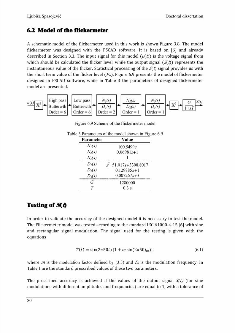
8/12/2019 Voltage fluctuation in industrial network and compensation measures
http://slidepdf.com/reader/full/voltage-fluctuation-in-industrial-network-and-compensation-measures 86/156
Ljubiša Spasojević Doctoral dissertation
6.2 Model of the flickermeter
A schematic model of the flickermeter used in this work is shown Figure 3.8. The model
flickermeter was designed
with the PSCAD software. It isbased on
[6] and already
described in Section 3.3. The input signal for this model (u (t )) is the voltage signal fromwhich should be calculated the flicker level, while the output signal (S (t )) represents the
instantaneous value of the flicker. Statistical processing of the S (t ) signal provides us with
the short term value of the flicker level (P st ). Figure 6.9 presents the model of flickermeterdesigned in PSCAD software, while in Table 3 the parameters of designed flickermeter
model are presented.
Figure 6.9 Scheme of the flickermeter model
Table 3 Parameters of the model shown in Figure 6.9
Parameter Value N 1(s)
N 2(s)
N 3(s)
100.5499s
0.06981s+1
1
D1(s)
D2(s)
D3(s)
s2+51.017s+3308.8017
0.129885s+1
0.007267s+1
G
T
1280000
0.3 s
Testing of t)
In order to validate the accuracy of the designed model it is necessary to test the model.
The Flickermeter model was tested according to the standard IEC 61000-4-15 [6] with sineand rectangular signal modulation. The signal used for the testing is given with theequations
() = sin(250) [1 + sin(250)], (6.1)
where m is the modulation factor defined by (3.3) and f m is the modulation frequency. In
Table 1 are the standard prescribed values of these two parameters.
The prescribed accuracy is achieved if the values of the output signal S(t) (for sinemodulations with different amplitudes and f requencies) are equal to 1, with a tolerance of
80

8/12/2019 Voltage fluctuation in industrial network and compensation measures
http://slidepdf.com/reader/full/voltage-fluctuation-in-industrial-network-and-compensation-measures 87/156
Ljubiša Spasojević Doctoral dissertation
±5% [6]. In Table 4 the values obtained from the test were shown, while in Figure 6.10
they are graphically represented. In Figure 6.10 it is clear that the deviations of S (t ) arewithin the prescribed limits, except for the first two and the last value . If we take a look at
Figure 3.1 it is clear that these
frequenciesdo not significantly influence the flicker level.
Table 4 The values of S (t ) obtained by tests
f m (Hz) S(t) f m (Hz) S(t)
0.5 0.750 10.5 1.012
1.0 0.875 11.0 1.010
1.5 0.925 11.5 1.007
2.0 0.925 12.0 1.005
2.5 0.975 13.0 1.000
3.0 0.991 14.0 0.995
3.5 0.991 15.0 0.993
4.0 0.993 16.0 0.995
4.5 1.011 17.0 0.9935.0 1.005 18.0 0.998
5.5 1.015 19.0 1.000
6.0 1.015 20.0 1.009
6.5 1.007 21.0 1.005
7.0 1.008 22.0 1.008
7.5 1.015 23.0 1.010
8.0 1.015 24.0 1.018
8.8 1.015 25.0 1.038
9.5
10.0
1.015
1.010
33.3 1.544
- -
Figure 6.10 Graphical overview of the values from Table 4
81
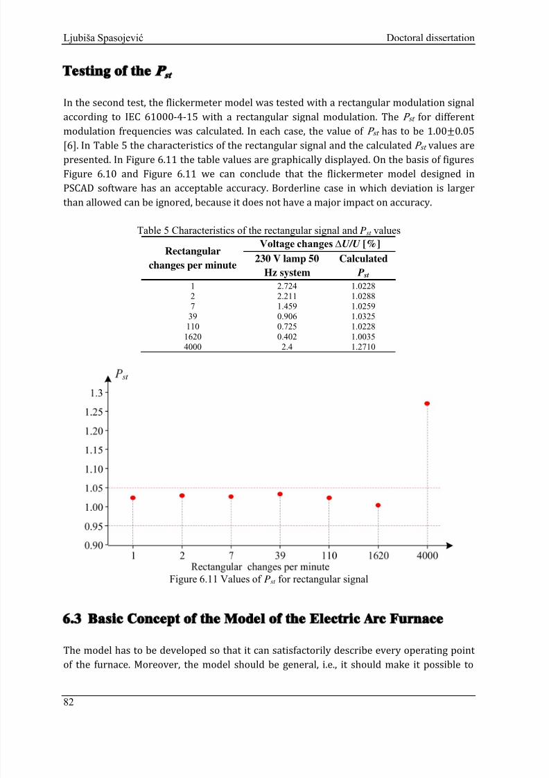
8/12/2019 Voltage fluctuation in industrial network and compensation measures
http://slidepdf.com/reader/full/voltage-fluctuation-in-industrial-network-and-compensation-measures 88/156
Ljubiša Spasojević Doctoral dissertation
Testing of thest
In the second test , the flickermeter model was tested with a rectangular modulation signal
according to IEC 61000-
4-
15 with a rectangular signal modulation. The P st for different
modulation frequencies was calculated. In each case, the value of P st has to be 1.00±0.05 [6]. In Table 5 the characteristics of the rectangular signal and the calculated P st values are
presented. In Figure 6.11 the table values are graphically displayed. On the basis of figuresFigure 6.10 and Figure 6.11 we can conclude that the flickermeter model designed inPSCAD software has an acceptable accuracy. Borderline case in which deviation is largerthan allowed can be ignored, because it does not have a major impact on accuracy. Table 5 Characteristics of the rectangular signal and Pst values
Rectangular
changes per minute
Voltage changes ∆U/U [%]
230 V lamp 50Hz system Calculated P st 1 2.724 1.0228
2 2.211 1.0288
7 1.459 1.0259
39 0.906 1.0325
110 0.725 1.0228
1620 0.402 1.0035
4000 2.4 1.2710
Figure 6.11 Values of Pst for rectangular signal
6.3 Basic Concept of the Model of the Electric Arc Furnace
The model has to be developed so that it can satisfactorily describe every operating pointof the furnace. Moreover, the model should be general, i.e., it should make it possible to82
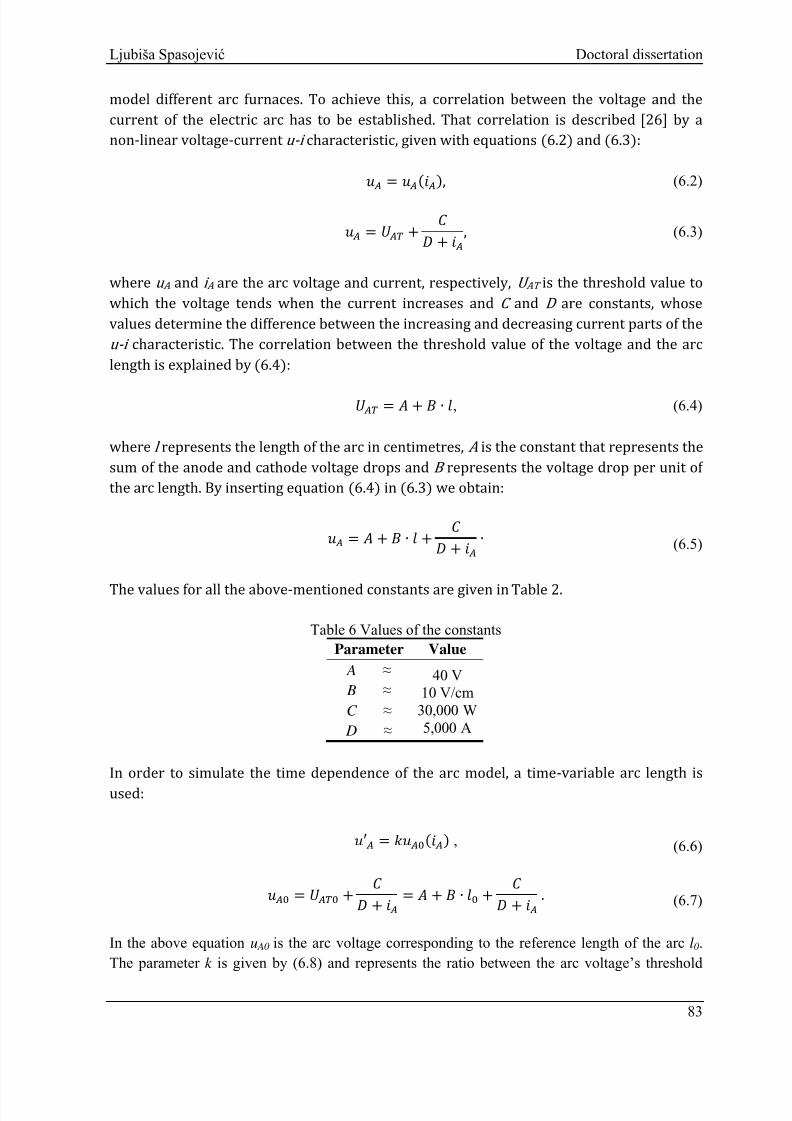
8/12/2019 Voltage fluctuation in industrial network and compensation measures
http://slidepdf.com/reader/full/voltage-fluctuation-in-industrial-network-and-compensation-measures 89/156
Ljubiša Spasojević Doctoral dissertation
model different arc furnaces. To achieve this, a correlation between the voltage and thecurrent of the electric arc has to be established. That correlation is described [26] by a
non-linear voltage-current u-i characteristic, given with equations (6.2) and (6.3):
= (), (6.2)
= + + , (6.3)
where u A and i A are the arc voltage and current, respectively, U AT is the threshold value to
which the voltage tends when the current increases and C and D are constants, whosevalues determine the difference between the increasing and decreasing current parts of the
u-i characteristic. The correlation between the threshold value of the voltage and the arc
length is explained by
(6.4):
= + ∙ , (6.4)
where l represents the length of the arc in centimetres, A is the constant that represents the
sum of the anode and cathode voltage drops and B represents the voltage drop per unit ofthe arc length. By inserting equation (6.4) in (6.3) we obtain:
=
+ ∙ +
+ ∙ (6.5)
The values for all the above-mentioned constants are given in Table 2.
Table 6 Values of the constants
Parameter Value A ≈
B ≈
C ≈
D ≈
40 V
10 V/cm
30,000 W
5,000 A
In order to simulate the time dependence of the arc model, a time-variable arc length isused: ′ = () , (6.6)
= + + = + ∙ + + . (6.7)
In the above equation u A0 is the arc voltage corresponding to the reference length of the arc l0.The parameter k is given by (6.8) and represents the ratio between the arc voltage’s threshold
83
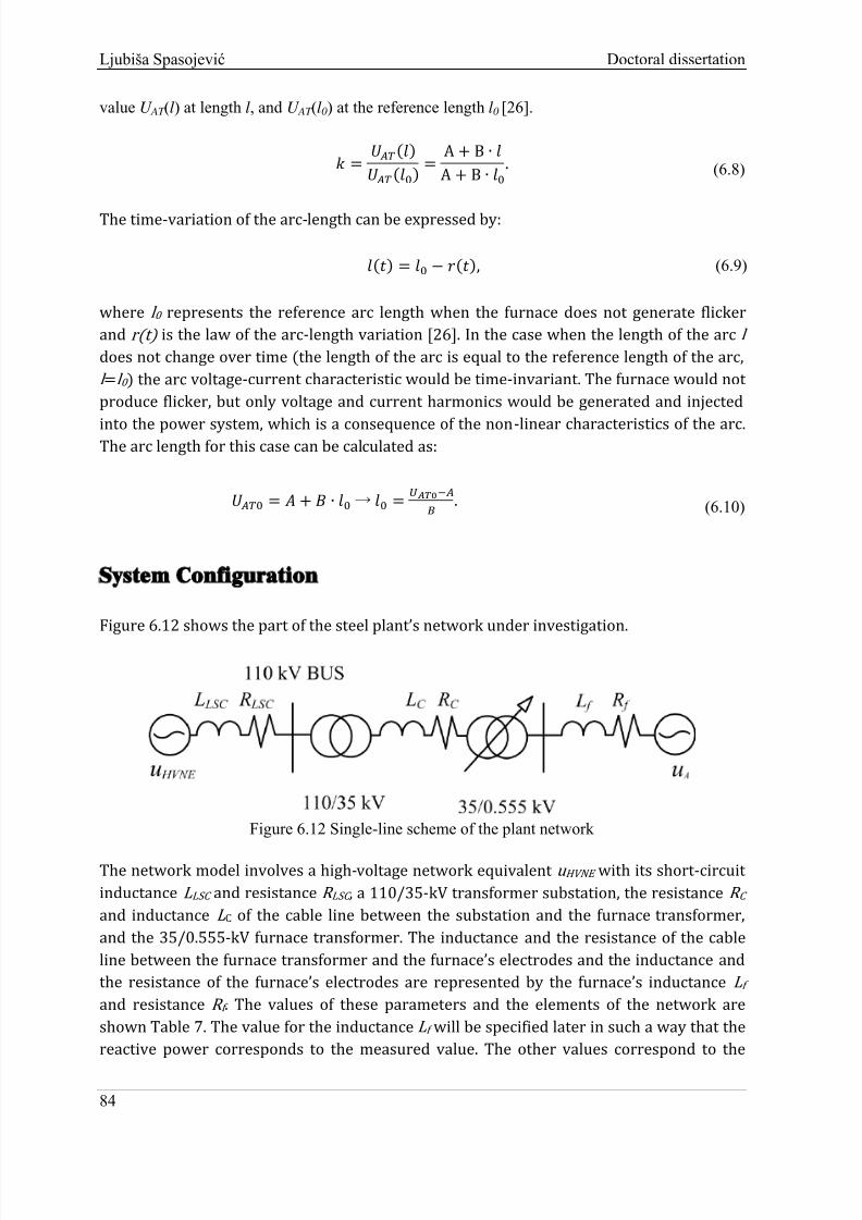
8/12/2019 Voltage fluctuation in industrial network and compensation measures
http://slidepdf.com/reader/full/voltage-fluctuation-in-industrial-network-and-compensation-measures 90/156
Ljubiša Spasojević Doctoral dissertation
value U AT (l) at length l, and U AT (l0) at the reference length l0 [26].
=()
(
) =
A + B ∙
A + B ∙ . (6.8)
The time-variation of the arc-length can be expressed by: () = (), (6.9)
where l 0 represents the reference arc length when the furnace does not generate flicker
and r(t) is the law of the arc-length variation [26]. In the case when the length of the arc l does not change over time (the length of the arc is equal to the reference length of the arc,l =l 0
) the arc voltage-current characteristic would be time-invariant. The furnace would not
produce flicker, but only voltage and current harmonics would be generated and injectedinto the power system, which is a consequence of the non-linear characteristics of the arc.
The arc length for this case can be calculated as: = + ∙ → =
− . (6.10)
System Configuration
Figure 6.12 shows the part of the steel plant’s network under investigation.
Figure 6.12 Single-line scheme of the plant network
The network model involves a high-voltage network equivalent u HVNE with its short-circuit
inductance L LSC and resistance R LSC , a 110/35-kV transformer substation, the resistance R C
and inductance L C of the cable line between the substation and the furnace transformer,and the 35/0.555-kV furnace transformer. The inductance and the resistance of the cableline between the furnace transformer and the furnace’s electrodes and the inductance and
the resistance of the furnace’s electrodes are represented by the furnace’s inductance L f
and resistance R f . The values of these parameters and the elements of the network are
shown Table 7. The value for the inductance L f will be specified later in such a way that thereactive power corresponds to the measured value. The other values correspond to the
84

8/12/2019 Voltage fluctuation in industrial network and compensation measures
http://slidepdf.com/reader/full/voltage-fluctuation-in-industrial-network-and-compensation-measures 91/156
Ljubiša Spasojević Doctoral dissertation
actual parameters of the steel plant. The short-circuit power S” sc at the 110-kV bus equals3750 MVA. Respecting the turn ratio of the transformers, all the measured values were
calculated at a low-voltage level.
Table 7 Values of the parameters of the model shown in Figure 6.12
Component Parameter Value
High-voltage
network equivalent
S’’sc
u HVNE
R/X
3750 MVA
110 kV
0.1
Tr 110/35
S tr1
untr1
uktr1
R/X
40 MVA
110/ 35 kV
10.49 %
0.1
Tr 35/0.555
S tr2
untr2
uktr2
R/X
35 MVA
35/0.555 kV
5.96 %0.1
Values of the parameters at 0.555 kV voltage level
cable resistancecable inductance
furnace resistance
R C
L C
R f
2.76∙10-6 Ω
1.31∙10-8 H
1.80∙10-3 Ω
The value of l 0 is calculated so that the furnace’s active power is the largest for every tapposition of the furnace transformer. This is achieved when the value of U AT0 is equal to 30%
of the voltage value (for that tap position) on the low-voltage side of the furnace
transformer. This correlation was determined experimentally based on real measured data.Since the furnace’s inductance L f is not known from the real factory network, its value wasalso determined experimentally based on the data from the selected representative sample
(P 1, Q 1). The values of these parameters were set such that the simulation model of theelectric arc furnace has approximately the same values of the active and reactive power as
the representative sample. Table 8 presents the experimentally determined parameters
based on real measured data.
Table 8 Values of experimentally determined parameters of the model used in the simulation Parameter of
Representative Sample ValueDetermined
Parameter Value
P1 12.62 MWU AT0
lo
167 V
12.84 cm
Q1 10.44 MVAr L f 8.02∙10-6 H
The law of the arc-length variation r (t ) in the case when the length of the arc l is not equalto the reference length of the arc l 0 but changes with time will be presented in the following
sections.
85

8/12/2019 Voltage fluctuation in industrial network and compensation measures
http://slidepdf.com/reader/full/voltage-fluctuation-in-industrial-network-and-compensation-measures 92/156
Ljubiša Spasojević Doctoral dissertation
Modeling the Electrical Arc Length
The basic idea of the proposed approach to modelling the electric arc furnace is that the
electrical arc is modelled as a controlled voltage source
[26]. This voltage source has to be
controlled so that it generates waveforms at the 110-kV level that correspond to thewaveforms of the representative (measured) samples. To achieve this, the amplitudes of all
the harmonic and interharmonic components of the voltage source have to be controlled.Therefore, the function F (f, A, φ ) (f – frequency, A – amplitude, φ – phase displacement ofinterharmonic) for control of the voltage source must be determined. This function, in fact,describes the arc-length variation.
All the resistances and reactances of the network in Figure 6.12 (of the 110/35-kV and
35/0.555-
kV transformers, of the cable and ofthe
furnace’s resistances andreactances
) canbe replaced with one equivalent resistance R eq and one equivalent reactance X eq , while theelectric arc furnace can be represented as a controlled voltage source. In this case, the
simplified single-line scheme shown in Figure 6.13 is obtained.
Figure 6.13 Simplified single-line scheme of the plant network
The waveforms of the voltage and current (i.e., the amplitudes and phase angles φ of all theharmonics and interharmonic components) at node B (measured at the 110-kV bus andrecalculated to the 0.555-kV level) are known from the measurements and arerepresentative samples of the voltage u RS and the current i RS . The voltage drop ∆u can be
calculated with (6.11) and, consequently, the waveforms of the voltage at point A can beobtained with (6.12). The voltage u A is the voltage at the point of the arc furnace’sconnection to the network.
∆ = ∙ ( + ), (6.11)
= ∙ ( + ) ∙ (6.12)
86

8/12/2019 Voltage fluctuation in industrial network and compensation measures
http://slidepdf.com/reader/full/voltage-fluctuation-in-industrial-network-and-compensation-measures 93/156
Ljubiša Spasojević Doctoral dissertation
Using the representative samples of voltage and current and the equivalent impedance, thevoltage waveforms at point A can be calculated. Equation (6.12) is an ordinary differentialequation that has to be solved numerically, because the data are given in discrete form. In
this way the obtained voltage waveforms at the point A correspond to the actual
waveforms at that point. The voltage drops in phases b and c are calculated in the sameway.
Next, it is necessary to define the law of the arc-length variation r (t ) in the case when thelength of the arc l is not equal to the reference length of the arc l 0 but changes with time.
This can be calculated from the voltage envelope of the representative sample spectrum.
The arc voltage value u A in (6.3) corresponds to the calculated voltage (frommeasurements) at point A in Figure 6.13. The arc current can be easily calculated
(respecting the turn ratio of the transformers) from measured representative samples ofthe current. The obtained voltage fluctuations at point A correspond to the actual voltagefluctuations at the 0.555-kV level. Since the voltage waveform at point A is known, thevoltage envelope at 0.555-kV can be calculated. Calculation of the Voltage Envelope
To calculate the voltage envelope of u A the squaring-demodulation method is used [37].
The structure of this method is shown in Figure 6.14, while Figure 6.15 and Figure 6.16
show the signal waveforms before and after passing through the squaring-demodulation
structure. The filter used in this case is a first-order high-pass filter with a cut-off frequencyof 3 dB at 0.05 Hz, while a 6th-order Butterworth low-pass filter has a cut-off frequency of3 dB at 35 Hz. The high-pass filter is used to eliminate the DC component and theButterworth filter to reject the double main frequency components caused by the squaringdemodulator, Figure 6.16. By applying a fast Fourier transform (FFT) to the signal p' (t ) aset of interharmonics (amplitudes A and phase angles φ ) for this signal are calculated. Asampling frequency for the FFT equal to 1 Hz was chosen.
Figure 6.14 Squaring-demodulation structure
The calculated set of interharmonics can be considered as being characteristic for each
individual installed furnace and therefore represents its fingerprint in the system. The
signal p (t ) is computed by applying an inverse fast Fourier transform (IFFT), covering thefrequency range from 1
Hz to 35
Hz, to the obtained set of interharmonics. Since this rangeof interharmonics involves all the important frequencies for flicker [38], [39] it will be used
87

8/12/2019 Voltage fluctuation in industrial network and compensation measures
http://slidepdf.com/reader/full/voltage-fluctuation-in-industrial-network-and-compensation-measures 94/156
Ljubiša Spasojević Doctoral dissertation
for modelling the time variation of the arc length r (t ) in (6.9). The obtained signal involves
all the signals with frequencies from 1 Hz to 35 Hz generated by the electric arc furnace
during its operation. In this way the interharmonics were calculated based on the data
from actual measurements.
Figure 6.15 Waveform input signal of the squaring-demodulation structure
Figure 6.16 Waveform output signal of the squaring-demodulation structure
6.4 The Results of the Simulation
A detailed three-phase model of an industrial network in a steel factory, shown in Figure
6.12, was designed with the PSCAD software. The network equivalent is represented with a
voltage source respecting the short-circuit power S” sc at the 110-kV bus. The non-linear
88

8/12/2019 Voltage fluctuation in industrial network and compensation measures
http://slidepdf.com/reader/full/voltage-fluctuation-in-industrial-network-and-compensation-measures 95/156
Ljubiša Spasojević Doctoral dissertation
arc-furnace model was implemented in the simulation program with three single-phase
controllable voltage sources. The control function F (f , A, φ ) for the control of the voltagesource at the arc-furnace model is based on equations (6.6) and can be written as:
= ′ = () ∙ (). (6.13)Substituting the calculated signal p (t ) in equation (6.9) the law of the arc-length variation
is derived. In order to achieve identical levels of flicker P st in the simulation and therepresentative sample, the signal p (t ) was multiplied by the constant G (gain), which wasdetermined experimentally (based on measured data) and was set to 6.25, equation (6.14).
() = ∙ (). (6.14)
Applying the above-mentioned equation (6.9) for the time-variation of the arc-lengthbecomes: () = ∙ (). (6.15)
Furthermore, based on the time-variation of the parameter k expressed by (6.8) and(6.15), the parameter k can be written as:
() = + ∙ (
) + ∙ = 1 ∙ ∙ (
) + ∙ . (6.16)
Finally, the equation that describes the control function F of the controllable voltage sources
representing the electric arc furnace model is given by:
= 1 ∙ ∙ () + ∙ ∙ + ∙ + + . 6.17)
A total simulation time (T
) of 50 seconds was chosen with a sampling frequency of 6.4 kHz.
In the simulation the waveforms of the voltage at the 110-kV and 0.555-kV levels wereobserved along with the flicker level at the 110-kV level. The interharmonics spectrum ofthe voltage at 110 kV, which is the cause of the flicker, is shown in Figure 6.17. Two sets of
interharmonic spectra are shown: the simulated and the measured. Although thedifferences in the amplitude between some interharmonics can be seen, both voltagescause approximately the same level of flicker at 110 kV. The amplitudes of the 50-Hz
component of the measured and obtained signals are identical and equal to 89.90 kV. InFigure 6.17 they are given with different lines because of the ordinate scaling.
89

8/12/2019 Voltage fluctuation in industrial network and compensation measures
http://slidepdf.com/reader/full/voltage-fluctuation-in-industrial-network-and-compensation-measures 96/156
Ljubiša Spasojević Doctoral dissertation
Figure 6.17 The spectrum of interharmonics at the 110-kV level; a) measured, b) simulated
The waveforms of the voltage and current simulated at the 0.555-kV level are shown in
Figure 6.18 and
Figure 6.19. These correspond to the waveforms of the voltage and the
current of the electrical arc.
Figure 6.18 Waveforms of the voltage simulated at the 0.555-kV level
90

8/12/2019 Voltage fluctuation in industrial network and compensation measures
http://slidepdf.com/reader/full/voltage-fluctuation-in-industrial-network-and-compensation-measures 97/156
Ljubiša Spasojević Doctoral dissertation
Figure 6.19 Waveforms of the current simulated at the 0.555-kV level
If we put the waveforms of the voltage and current simulated at the 0.555 -kV level in thesame figure, Figure 6.20, it is clear that there are no phase displacements between them.Also, it is clear that irrespective of the polarity of the voltage, t he arc remains permanently
conductive. In Figure 6.20 the voltage of the arc u A is given in volts, while the arc current isgiven in kiloamperes.
Figure 6.20 Simulated waveform of the voltage u A and the waveform of the current i A of the
electrical arc
The absence of a phase shift between the arc voltage and thearc current, and the fact that
the arc contains only ohmic resistance was confirmed. Based on all these simulation
results, the obtained arc voltage-current u-i characteristic of this electric arc furnace model
is shown in Figure 6.21.
91

8/12/2019 Voltage fluctuation in industrial network and compensation measures
http://slidepdf.com/reader/full/voltage-fluctuation-in-industrial-network-and-compensation-measures 98/156
Ljubiša Spasojević Doctoral dissertation
Figure 6.21 Dynamic voltage-current u-i characteristic obtained from the simulation results
The time variation of the arc length l obtained with this method and the reference length of
the arc l 0 are shown in Figure 6.22.
Figure 6.22 Reference arc length l0 and the arc length obtained in the simulation l
92

8/12/2019 Voltage fluctuation in industrial network and compensation measures
http://slidepdf.com/reader/full/voltage-fluctuation-in-industrial-network-and-compensation-measures 99/156
Ljubiša Spasojević Doctoral dissertation
In the picture it is clear that the main characteristic of the electric arc is fast and largechanges of the length in a very short period of time. Also, the picture clearly shows that atany point the arc length is not equal to 0. Based on that can be concluded that the electricarc is uninterrupted.
Figure 6.23 shows a representative sample’s instantaneous values of the flicker S (t ) at the110-kV level together with the simulated values. It is clear that the waveforms of these two
signals are approximately the same. After the statistical processing of both signals,approximately the same value of P st was obtained, as shown in Table 9.
Figure 6.23 Representative sample’s S (t ) RS and simulated S (t )sim instantaneous values of flickerat the 110-kV level
The simulated flicker level P st, sim , the flicker level of a representative sample P st, r and theflicker level measured at 110 kV P st are shown in Table 9; the measured active and reactive
power (P m , Q m ), active and reactive power of representative sample (P 1 , Q 1 ) and thesimulated values (P sim , Q sim ) are shown in the same table.
Table 9 Values of active power, reactive power and flicker level
Parameter ValuePst
Pst, r
Pst, sim
1.450
1.453
1.457
Pm
P1
Psim
13.49 MW
12.62 MW
12.62 MW
Qm
Q1
Qsim
10.09 MVAr
10.44 MVAr
10.44 MVAr
93

8/12/2019 Voltage fluctuation in industrial network and compensation measures
http://slidepdf.com/reader/full/voltage-fluctuation-in-industrial-network-and-compensation-measures 100/156
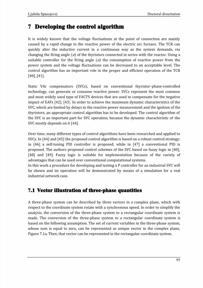
8/12/2019 Voltage fluctuation in industrial network and compensation measures
http://slidepdf.com/reader/full/voltage-fluctuation-in-industrial-network-and-compensation-measures 101/156
Ljubiša Spasojević Doctoral dissertation
7 Developing the control algorithm
It is widely known that the voltage fluctuations at the point of connection are mainly
caused by a rapid change in the reactive power of the electric arc furnace. The
TCR canquickly alter the inductive current in a continuous way as the system demands, viachanging the firing angle (α ) of the thyristors connected in series with the reactor. Using a
suitable controller for the firing angle (α ) the consumption of reactive power from the
power system and the voltage fluctuations can be decreased to an acceptable level. The
control algorithm has an important role in the proper and efficient operation of the TCR [40], [41].
Static VAr compensators (SVCs), based on conventional thyristor-phase-controlled
technolog
y, can generate or consume reactive power. SVCs represent the most commonand most widely used type of FACTS devices that are used to compensate for the negativeimpact of EAFs [42], [43]. In order to achieve the maximum dynamic characteristics of theSVC, which are limited by delays in the reactive power measurement and the ignition of thethyristors, an appropriate control algorithm has to be developed. The control algorithm ofthe SVC is an important part for SVC operation, because the dynamic characteristic of theSVC mostly depends on it [44].
Over time, many different types of control algorithms have been researched and applied to
SVCs. In
[44] and
[45] the proposed control algorithm is based on a robust control strategy
:
in [46] a self-tuning PID controller is proposed, while in [47] a conventional PID isproposed. The authors proposed control schemes of the SVC based on fuzzy logic in [40], [48] and [49]. Fuzzy logic is suitable for implementation because of the variety of
advantages that can be used over conventional computational systems.
In this work a procedure for developing and testing a P controller for an industrial SVC willbe shown and its operation will be demonstrated by means of a simulation for a real
industrial network case.
7.1 Vector illustration of three-phase quantities
A three-phase system can be described by three vectors in a complex plane, which with
respect to the coordinate system rotate with a synchronous speed. In order to simplify the
analysis, the conversion of the three-phase system to a rectangular coordinate system is
made. The conversion of the three-phase system to a rectangular coordinate system is
based on the following assumption. The set of current variables in the three-phase system, whose sum is equal to zero, can be represented as unique vector in the complex plane,Figure 7.1a. Then, that vector can be represented in the rectangular coordinate system.
95
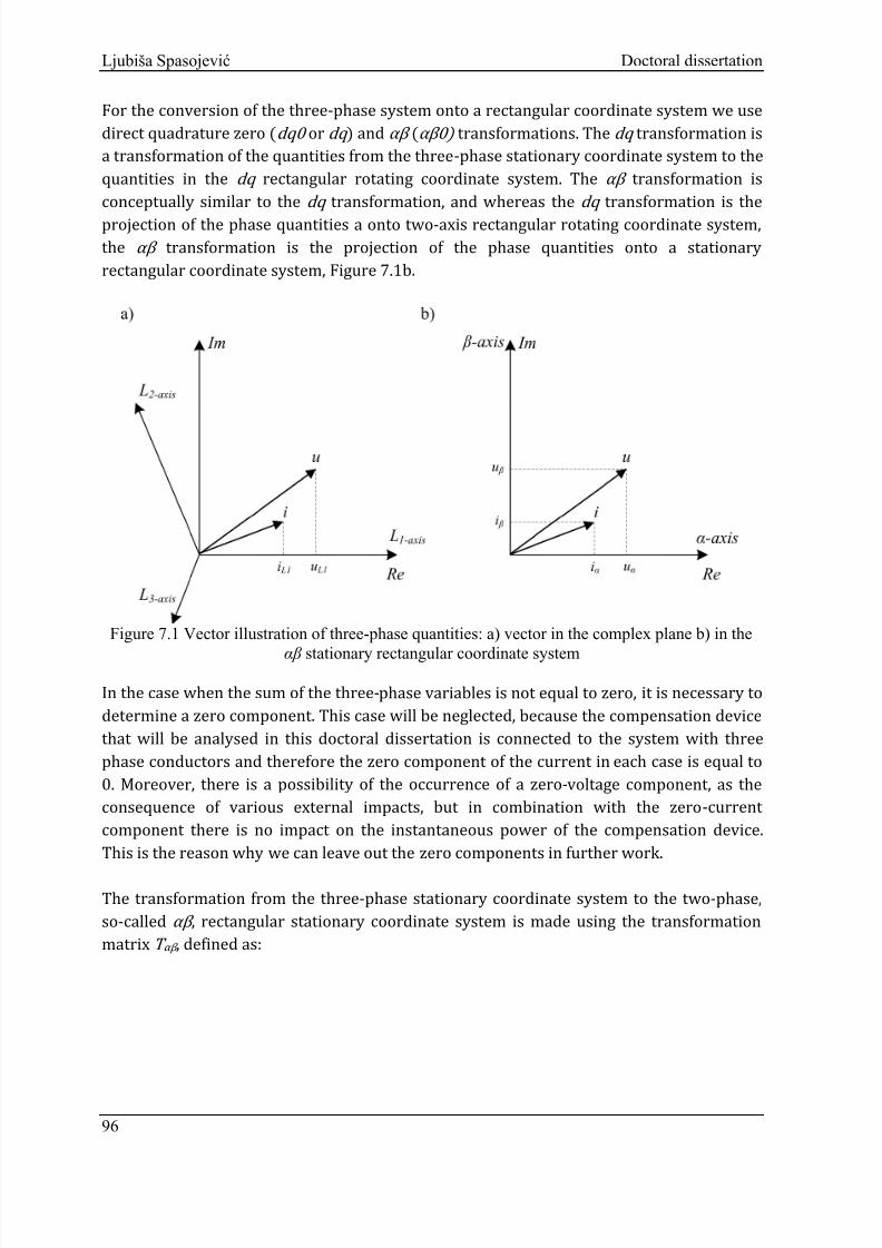
8/12/2019 Voltage fluctuation in industrial network and compensation measures
http://slidepdf.com/reader/full/voltage-fluctuation-in-industrial-network-and-compensation-measures 102/156
Ljubiša Spasojević Doctoral dissertation
For the conversion of the three-phase system onto a rectangular coordinate system we usedirect quadrature zero (dq0 or dq ) and αβ (αβ0) transformations. The dq transformation is
a transformation of the quantities from the three-phase stationary coordinate system to the
quantities inthe dq rectangular rotating coordinate system. The αβ transformation is
conceptually similar to the dq transformation, and whereas the dq transformation is theprojection of the phase quantities a onto two-axis rectangular rotating coordinate system,the αβ transformation is the projection of the phase quantities onto a stationaryrectangular coordinate system, Figure 7.1b.
Figure 7.1 Vector illustration of three-phase quantities: a) vector in the complex plane b) in theαβ stationary rectangular coordinate system
In the case when the sum of the three-phase variables is not equal to zero, it is necessary to
determine a zero component. This case will be neglected, because the compensation devicethat will be analysed in this doctoral dissertation is connected to the system with three
phase conductors and therefore the zero component of the current in each case is equal to0. Moreover, there is a possibility of the occurrence of a zero-voltage component, as theconsequence of various external impacts, but in combination with the zero-current
component there is no impact on the instantaneous power of the compensation device.
This is the reason why we can leave out the zero components in further work.
The transformation from the three-phase stationary coordinate system to the two-phase,so-called αβ , rectangular stationary coordinate system is made using the transformationmatrix T αβ , defined as:
96
8/12/2019 Voltage fluctuation in industrial network and compensation measures
http://slidepdf.com/reader/full/voltage-fluctuation-in-industrial-network-and-compensation-measures 103/156
Ljubiša Spasojević Doctoral dissertation
α =23
⎣
1 12 120 √ 32 √ 3212 12 12 ⎦
. (7.1)
The variables of the αβ coordinate system are calculated from the variables of the three-
phase system as follows:
= and = . (7.2)
The calculated components α and β represent the vector projection to the perpendicularaxis, Figure 7.1b. From the obtained α and β components of the voltage and current (i αβ , u αβ ), the amplitudes can be calculated using the following equations:
= α + β (7.3)
and
=
α + β .
(7.4)
The transformation from the three-phase stationary coordinate system to the two-phase,so-called dq transformation, rectangular rotating coordinate system is made using thetransformation matrix T dq , defined as
=
23 ⎣
⎡
cos() cos 23 cos + 23 sin(
) sin
23
sin
+23 12 12 12 ⎦
⎤. (7.5)
The variables of the dq coordinate system are calculated from the variables of the three-
phase system as follows
=
and = . (7.6)
In the conversion to the dq rotating coordinate system it is necessary to indicate that thetransformation matrix is no longer constant. Now, the transformation matrix is time-
97

8/12/2019 Voltage fluctuation in industrial network and compensation measures
http://slidepdf.com/reader/full/voltage-fluctuation-in-industrial-network-and-compensation-measures 104/156
Ljubiša Spasojević Doctoral dissertation
dependent and as a variable contains the angular speed ω . The angular speed represents
the synchronous speed of the rotating dq coordinate system. A vector illustration in the
two-phase synchronous rotating coordinate system is shown Figure 7.2b.
Figure 7.2 Vector illustration of three-phase quantities: a) vector in the complex plane b) in the
dq rotating coordinate system
The transformation to the dq rectangular rotating coordinate system gets real practicalvalue when the angular speed of the dq coordinate system is equal to the angular speed ofthe three-phase system. In such a case, the AC quantities, voltage and current, in the three-phase AC system are converted to the constant quantities of the dq rotating coordinate
system (only in steady-state conditions). This property is very suitable for thedevelopment of a control algorithm for system devices.
Instantaneous active and reactive power
The instantaneous active power in the three-phase system quantities can be calculated
using the following equation: () = ()( ) + ()()+()(). (7.7)
The instantaneous reactive power can be described as part of the power that exists in eachphase and whose sum of all three phases is equal to zero. Because of it, there is no influenceof the instantaneous reactive power on the instantaneous active power.
98

8/12/2019 Voltage fluctuation in industrial network and compensation measures
http://slidepdf.com/reader/full/voltage-fluctuation-in-industrial-network-and-compensation-measures 105/156
Ljubiša Spasojević Doctoral dissertation
Using the transformation matrix (7.1) the instantaneous active and reactive power can be
written in the αβ rectangular coordinate system as:
=
32 α
α
+ β
β
, (7.8)
=32 α β + β α . (7.9)
In the same way, using the transformation matrix (7.5) the instantaneous active and
reactive power can be written in the dq rectangular rotating coordinate system as:
=
32
+
, (7.10)
=32 + . (7.11)
If we make an appropriate synchronization of the dq rectangular rotating coordinatesystem, the value of u q will be:
=
0. (7.12)
This synchronization is achieved when the angle (φ ) between the voltage vector of phaseL 1 and d -axe of the dq rotating coordinate system is equal to 0. According to all the
mentioned equations for the instantaneous active and reactive power in the dq coordinate
system become: =
32 , (7.13)
= 32 . (7.14)
On the basis of (7.14), we can conclude that the q -component of the current is proportionalto the reactive power, while the d -component is proportional to the active power.
99
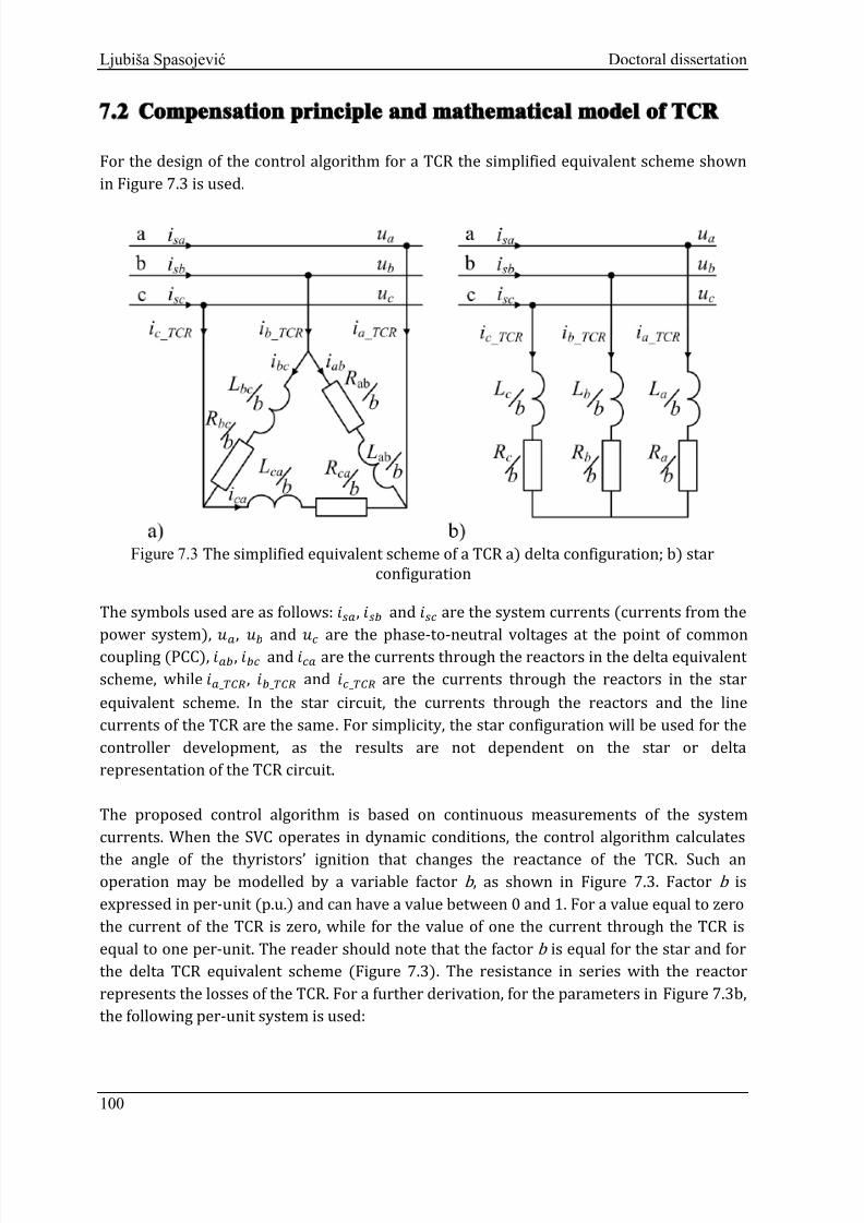
8/12/2019 Voltage fluctuation in industrial network and compensation measures
http://slidepdf.com/reader/full/voltage-fluctuation-in-industrial-network-and-compensation-measures 106/156
Ljubiša Spasojević Doctoral dissertation
7.2 Compensation principle and mathematical model of TCR
For the design of the control algorithm for a TCR the simplified equivalent scheme shownin
Figure 7.3 is used.
Figure 7.3 The simplified equivalent scheme of a TCR a) delta configuration; b) starconfiguration
The symbols used are as follows: , and are the system currents (currents from thepower system), , and are the phase-to-neutral voltages at the point of commoncoupling (PCC), , and are the currents through the reactors in the delta equivalentscheme, while _, _ and _ are the currents through the reactors in the starequivalent scheme. In the star circuit, the currents through the reactors and the linecurrents of the TCR are the same . For simplicity, the star configuration will be used for thecontroller development, as the results are not dependent on the star or deltarepresentation of the TCR circuit. The proposed control algorithm is based on continuous measurements of the systemcurrents. When the SVC operates in dynamic conditions, the control algorithm calculatesthe angle of the thyristors’ ignition that changes the reactance of the TCR. Such anoperation may be modelled by a variable factor b , as shown in Figure 7.3. Factor b is
expressed in per-unit (p.u.) and can have a value between 0 and 1. For a value equal to zerothe current of the TCR is zero, while for the value of one the current through the TCR isequal to one per-unit. The reader should note that the factor b is equal for the star and forthe delta TCR equivalent scheme (Figure 7.3). The resistance in series with the reactorrepresents the losses of the TCR. For a further derivation, for the parameters in Figure 7.3b,the following per-unit system is used
:
100

8/12/2019 Voltage fluctuation in industrial network and compensation measures
http://slidepdf.com/reader/full/voltage-fluctuation-in-industrial-network-and-compensation-measures 107/156
Ljubiša Spasojević Doctoral dissertation
=_ , =
_ , =_ , (7.15)
=
, =
, =
, (7.16)
= , =
, = , (7.17)
= , =
, = , =
, (7.18)
where
, and
are the base values of the current, voltage and impedance,respectively, while is the synchronous angular speed of the fundamental networkcomponent. When the per-unit system is adopted, the following set of equations can bewritten, based on the equivalent scheme shown in Figure 7.3b:
= _ + ,
= _ + ,
= _ +
(7.19)
or on p.u.: =
+ ,
=
+
,
=
+ .
(7.20)
Applying the dq transformation, a 3-phase system can be transformed into a dq synchronous rotation coordinate system (SRCS). Assuming that the phase inductances andphase resistances are equal (
X and R
respectively), equation (7.19) can be written as (7.21)in d-q SRCS and using the Laplace transform.
101

8/12/2019 Voltage fluctuation in industrial network and compensation measures
http://slidepdf.com/reader/full/voltage-fluctuation-in-industrial-network-and-compensation-measures 108/156
Ljubiša Spasojević Doctoral dissertation
+ ′X′
=X′
+ (7.21)
where s=d/dt . In this case both components (
and
) of the current that flows into theTCR are coupled by the angular speed ω . A common choice would also be to set = .In steady-state conditions the values of and are constant, which is convenient for thederivation of the control algorithm. The currents can be expressed as:
+ ′X′
=X′
+ , (7.22)
+ ′
′
=
′
, (7.23)
= 1 + ′X′
X′
+ , (7.24)
=1
+ ′ ′ ′ .
(7.25)
Based on equations (7.24) and (7.25) a simplified mathematical model ofthe
TCR device ind q SRCS is obtained and is shown in Figure 7.4.
Figure 7.4 Simplified mathematical model of TCR
102

8/12/2019 Voltage fluctuation in industrial network and compensation measures
http://slidepdf.com/reader/full/voltage-fluctuation-in-industrial-network-and-compensation-measures 109/156
Ljubiša Spasojević Doctoral dissertation
7.3 Controller design
The derivation of the control algorithm of the TCR device in the d-q SRCS starts from the
simplified mathematical model shown in
Figure 7.4. Firstly,a proper synchronization of the
coordinate system must be made. With this proper synchronization the reactivecomponent ( ) of the TCR current is proportional to the reactive power (q ) of the TCRdevice. The d q SRCS is synchronized to the medium-voltage (MV) level so that the angle φ
between the voltage vector of u MV (voltage at the MV level) and the d-axes of the d q SRCS equals 0.From Figure 7.4 it is clear that a change in the factor b influences the value of . Therefore,the desired values of can be generated by suitable values of the factor b . In fact, thes
usceptance of the TCR (B TCR
) can be controlled by the parameterb .
Now, the connection between the reactive component of the TCR current () and thereactive component of the system current () should be established. The system current() flows from the power system to the EAF and its reactive component should becompensated to zero. Figure 7.5 shows a simplified system configuration.
Figure 7.5 Simplified scheme of the system
For point A we can write:
= , (7.26)
where , and are the system current, the SVC current and the load current,respectively. Subsequently, the current of the SVC device (i svc ) can be written as: = + , (7.27)
where
and
are the TCR and FC currents. Based on equations (7.26) and
(7.27), thereactive current components of the system current () and of the SVC device () inthe d q SRCS are obtained:
103

8/12/2019 Voltage fluctuation in industrial network and compensation measures
http://slidepdf.com/reader/full/voltage-fluctuation-in-industrial-network-and-compensation-measures 110/156
Ljubiša Spasojević Doctoral dissertation
In a fully compensated system, the reactive component of the system current () shouldbe equal to zero. In other words, the reactive component of the TCR current should beadjusted so that equals zero:
In this way, when the TCR controller regulates the system current () to zero, the reactivecomponent of the load current () is fully compensated, as follows from equation (7.30).
Figure 7.6 shows the control scheme in the dq frame. Proportional–integral (PI) controllersare used in this control algorithm to set the reference for the P controller. Only one of the
two PI controllers is used for setting the reference. The choice depends on the aim of theregulation (voltage, reactive power or flicker control). The power and the voltage
represent the instantaneous values of the reactive power and the
RMS voltage at the
MV level. The reference current ∗ is compared to the q -component of the system
current .
Figure 7.6 Basic idea for the design of the control algorithm,
= , (7.28)
= + , (7.29)
+ = 0 →
→ =
(
)
(7.30)
104
8/12/2019 Voltage fluctuation in industrial network and compensation measures
http://slidepdf.com/reader/full/voltage-fluctuation-in-industrial-network-and-compensation-measures 111/156
Ljubiša Spasojević Doctoral dissertation
The control algorithm is based on the continuous monitoring and computing of the reactivecurrent from the power system. The frequency range of 0.5 to 35 Hz should be extractedfrom the whole spectrum of the reactive current since this frequency spectrum ( with
observable magnitudes starting at less than 1.0
%) represents the main source of theflicker phenomena [50], [51]. Frequencies outside this range should not influence theoperation of the controller because they could reduce its efficiency to reduce the flicker.
This can be achieved by filtering the input signals of the P controller. In this study filtersbased on a fast Fourier transform (FFT) were used. Based on the actual values of the inputs, the control algorithm calculates the required valueof the susceptance (B TCR ) in p.u. A correlation between the susceptance B TCR and the firing
angle α is nonlinear and is described by the following equation [52]:
= 22+2 , (7.31)
where X L represents the maximum reactance of the TCR. By changing the susceptance ofthe B TCR , the RMS value of the current through the reactor is changed and can be expressedas a function of the firing angle as follows:
= (22+2), (7.32)
where U rms is the RMS value of the connected voltage, L is the inductance of the TCR, and ω is the angular frequency of the voltage at the connection point [53].
Transfer function of the P controller
The transfer function of the P controller from Figure 7.6 can be expressed as follows:
where ∗ represents the reference value of the reactive current component on the MV level,while is the measured value of the reactive component of the total system current ().It should be noted that = , as already shown. Subsequently, the response time of the TCR (T TCR ) is limited by the thyristor’s ignitiondelay [52]. Namely, the thyristor phase angle can be varied once during each half-cycle (in
each phase). The ignition delay is not fixed and depends on the instant of the referencechange (thyristor dead-time) and the delay between the sampling instant and the instantwhen the thyristor starts to conduct (firing delay). The required frequency of changing the
= ∗ , (7.33)
105

8/12/2019 Voltage fluctuation in industrial network and compensation measures
http://slidepdf.com/reader/full/voltage-fluctuation-in-industrial-network-and-compensation-measures 112/156
Ljubiša Spasojević Doctoral dissertation
value of the parameter b is six times the fundamental frequency for a three-phase 6-pulseTCR. In order to model the TCR delay, the parameter b should be multiplied by a first-order
block with the time constant T TCR representing the average delay time, as shown in
equation (7.34).
= ′1 + . (7.34)
Taking into account equation (7.33) we obtain: =
∗ (1 + ). (7.35)
By using equation (7.35), a direct connection between the controller output and themathematical model of the TCR is established. Based on this definition of the parameter b' ,and taking intoaccount equations (7.24), (7.25) and (7.35), the following set of equations isobtained for the TCR current: =
1 + ′ ′
∗ 1 + ′ + ,
(7.36)
= 1 + ′ ′ ∗ 1 + ′ , (7.37)
where , are the d- and q - components of the measured voltage at the SVC connectionpoint. This set of equations represents the mathematical model of a TCR controlled with a Pcontroller. The block diagram of the mathematical model can be seen in Figure 7.7.
106

8/12/2019 Voltage fluctuation in industrial network and compensation measures
http://slidepdf.com/reader/full/voltage-fluctuation-in-industrial-network-and-compensation-measures 113/156
Ljubiša Spasojević Doctoral dissertation
Figure 7.7 The simplified mathematical model of the TCR with the P controller
7.4 Model testing
The static analysis
In order to analyse the static accuracy, the dynamic accuracy and the stability of this model,its transfer function has to be determined. By inserting equation (7.36) into (7.37) the
transfer functions of the system shown in Figure 7.7 are calculated as follows (equations(7.38) and (7.39)): =
1 +
⎣∗ 1 + ∙ 1
+ ∗ 1 + ∙ +
⎦. (7.38)
= + + (1 + 2 ) + 2 + + + + ,
where:
=
, =
, =
. (7.40)
x
ω
ω
R' ω b
X' s +
1
R' ω b
X' s +
1
id
iq
K piq b
ω b
X'
ω b
X' x
1
1+sT TCR
'
'
'* b'
ud '
uq '
() = ∗ = (7.39)
107

8/12/2019 Voltage fluctuation in industrial network and compensation measures
http://slidepdf.com/reader/full/voltage-fluctuation-in-industrial-network-and-compensation-measures 114/156

8/12/2019 Voltage fluctuation in industrial network and compensation measures
http://slidepdf.com/reader/full/voltage-fluctuation-in-industrial-network-and-compensation-measures 115/156

8/12/2019 Voltage fluctuation in industrial network and compensation measures
http://slidepdf.com/reader/full/voltage-fluctuation-in-industrial-network-and-compensation-measures 116/156
Ljubiša Spasojević Doctoral dissertation
Figure 7.8 The step response of the system; 1 – response of the real TCR model; 2 – response of
the mathematical model for the case T TCR=6 ms; 3 – response of the mathematical model for the
case T TCR=4 ms; 4 – response of the mathematical model for the case T TCR=2 ms
The stability was tested using the Bode stability criterion. According to this criterion, a
closed-loop system will be stable if the value of the gain is less than 1 at the criticalfrequency. The critical frequency is equal to -180 degrees. The obtained results are shownin Figure 7.9. Based on Figure 7.9 it can be concluded that the system will be stable for the
selected parameters K p and T TCR .
110

8/12/2019 Voltage fluctuation in industrial network and compensation measures
http://slidepdf.com/reader/full/voltage-fluctuation-in-industrial-network-and-compensation-measures 117/156
Ljubiša Spasojević Doctoral dissertation
Figure 7.9 Bode diagram of F(s)tr for values of T TCR = 0.004 s and K p=0.50;
7.5 The simulation results
The SVC control system proposed in this work has been applied for the realistic model of a
steel factory. The electric arc furnace is modelled as described in Chapter 6. The control
function F of the controllable voltage sources is described by (6.17).
Firstly, f or modelling the time variation of the electric arc length a sinusoidal function with
different frequencies was used. Frequencies of 5, 9 and 13 Hz were used. For this case,equation (6.17),
which defines the control function of the controllable voltage sources
,
becomes: = 1 ∙ ∙ (2 ) + ∙ ∙ + ∙ + + , (7.48)
where f sin can have values of 5, 9 or 13 Hz. Since the frequency of 9 Hz is the worst for theflicker production, waveform of simulated data only for this frequency will be graphicalpresented. For other frequencies the simulated data will only be presented numerically.
After simulations with the sinusoidal function for modelling the time variation of theelectric arc length, simulations with a signal that involves all the important frequencies for
111

8/12/2019 Voltage fluctuation in industrial network and compensation measures
http://slidepdf.com/reader/full/voltage-fluctuation-in-industrial-network-and-compensation-measures 118/156
Ljubiša Spasojević Doctoral dissertation
flicker were made. The calculation procedure for this signal is described in Chapter 6. Theequation (6.17) describes the control function of the controllable voltage sources used in
this case. In each simulated case the parameters of the electric arc furnace model were
adjusted so that the model generated the same level of flicker (P st
) at 110 kV. The modelwas calibrated according to the field measurements.
The system configuration
In Figure 7.10 a simplified single-line diagram of the steel plant’s network underinvestigation is shown. The network model involves a high-voltage network equivalentwith its short-circuit inductance (L LSC ) and resistance (R LSC ), a 110/35-kV transformersubstation, the resistance (R C ) and inductance (L C ) of the cable line between the substationand the furnace
transformer, the 35/0.74-
kV furnace transformer and inductance (L f
) and
the resistance (R f ) of the cable line between the furnace transformer and the furnace
electrodes.
Figure 7.10 Single-line scheme of the plant network
The values of these parameters are shown in Table 10 and correspond to the actual
parameters of the steel plant. The short-circuit power (S’’ sc ) at the 110-kV bus equals3200 MVA.
112
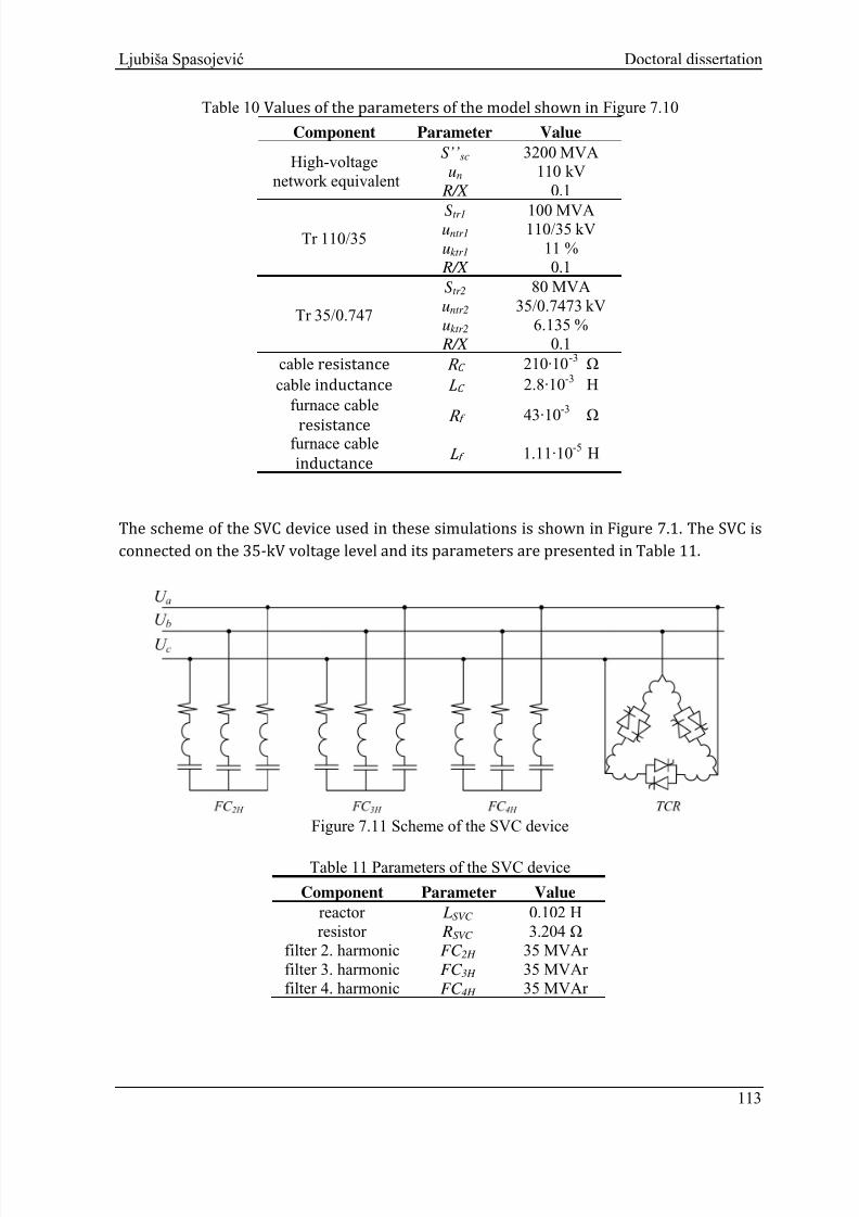
8/12/2019 Voltage fluctuation in industrial network and compensation measures
http://slidepdf.com/reader/full/voltage-fluctuation-in-industrial-network-and-compensation-measures 119/156
Ljubiša Spasojević Doctoral dissertation
Table 10 Values of the parameters of the model shown in Figure 7.10
Component Parameter Value
High-voltage
network equivalent
S’’sc
un
R/X
3200 MVA
110 kV
0.1
Tr 110/35
S tr1
untr1
uktr1
R/X
100 MVA110/35 kV
11 %
0.1
Tr 35/0.747
S tr2
untr2
uktr2
R/X
80 MVA
35/0.7473 kV
6.135 %
0.1
cable resistance R C 210∙10-3 Ω
cable inductance L C 2.8∙10-3 H
furnace cableresistance
R f 43∙10-3 Ω
furnace cable
inductance L f 1.11∙10-5 H
The scheme of the SVC device used in these simulations is shown in Figure 7.1. The SVC isconnected on the 35-kV voltage level and its parameters are presented in Table 11.
Figure 7.11 Scheme of the SVC device
Table 11 Parameters of the SVC device
Component Parameter Valuereactor
resistor
filter 2. harmonic
filter 3. harmonic
filter 4. harmonic
LSVC
RSVC
FC 2H
FC 3H
FC 4H
0.102 H
3.204 Ω
35 MVAr
35 MVAr
35 MVAr
113

8/12/2019 Voltage fluctuation in industrial network and compensation measures
http://slidepdf.com/reader/full/voltage-fluctuation-in-industrial-network-and-compensation-measures 120/156
Ljubiša Spasojević Doctoral dissertation
7.6 Modelling of the electric-arc length using sinusoidal
function
Simulations without a connected SVC
A simulation of the steel-factory model without the SVC was carried out. A total simulation
time (T ) of 20 seconds was chosen, with a sampling time of 15 µs. Waveforms of the
simulated signals (frequency of arc length modulation 9 Hz), active (P ) and reactive (Q )powers of the furnace, are shown in Figure 7.12. P furnace and Q furnace represent the active and
reactive powers of arc furnace, respectively, measured on the low-voltage side of the
furnace transformer. The figure shows fluctuations of the active and reactive powers.These oscillations have a frequency of 9 Hz, and through the furnace transformer aretransferred to the medium-voltage level.
Furthermore, over the substation transformerthese oscillations are farther transferred to the 110-kV voltage level.
Figure 7.12 Simulated signals of the active and reactive powers without the connected SVC at
the low-voltage level of the furnace transformer (frequency of the arc-length modulation 9 Hz)
Figure 7.13 and Figure 7.14 show the simulated signals of the active and reactive powers
that are obtained at different voltage levels. Figure 7.13 shows the simulated signal of the
active and reactive powers at the medium-voltage level, while Figure 7.14 shows the same
simulated signal at the 110-kV level. If we compare Figure 7.14 and Figure 7.12 it is clear
that there are differences between the quantities of active and reactive powers
downloaded from the power system and consumed in the arc furnace. This differencerepresents the quantity of energy that is required to cover the losses in the transformers
and the cables.
114

8/12/2019 Voltage fluctuation in industrial network and compensation measures
http://slidepdf.com/reader/full/voltage-fluctuation-in-industrial-network-and-compensation-measures 121/156
Ljubiša Spasojević Doctoral dissertation
Figure 7.13 Simulated signals of the active and reactive powers of the furnace without the SVC
at the 35-kV level (frequency of arc length modulation 9 Hz)
Figure 7.14 Simulated signals of the active and reactive powers without the connected SVC at
the 110-kV voltage level (frequency of the arc-length modulation 9 Hz)
Furthermore, in the next figures (Figure 7.15-Figure 7.22) are the waveforms of otherquantities obtained by simulations. Figure 7.15 and Figure 7.17 show the waveforms of thevoltage and current, respectively, at the medium-voltage level. If we look carefully at Figure7.15 we can see fluctuations of the peak value of the voltage. These fluctuations can be
easily seen if we look at the waveform of RMS value of this voltage. The waveform of theRMS voltage value at the medium-voltage level is shown in Figure 7.16.
115

8/12/2019 Voltage fluctuation in industrial network and compensation measures
http://slidepdf.com/reader/full/voltage-fluctuation-in-industrial-network-and-compensation-measures 122/156
Ljubiša Spasojević Doctoral dissertation
Figure 7.15 Waveform of the voltage at the medium-voltage level without the SVC (frequency of
the arc-length modulation 9 Hz)
Figure 7.16 Fluctuations of the RMS voltage at the medium-voltage level (frequency of the arc-
length modulation 9 Hz)
The current waveforms at the medium-voltage level are presented in Figure 7.17.
116

8/12/2019 Voltage fluctuation in industrial network and compensation measures
http://slidepdf.com/reader/full/voltage-fluctuation-in-industrial-network-and-compensation-measures 123/156
Ljubiša Spasojević Doctoral dissertation
Figure 7.17 Waveform of the current at the medium-voltage level without the SVC (frequency of
the arc-length modulation 9 Hz)
The phase displacement between the voltage and the current at the medium voltage level
without the SVC can be seen in Figure 7.18.
Figure 7.18 Phase shift between the voltage and current at the medium-voltage level without the
SVC
The waveforms of the voltage and the current at the 110-kV level are shown in Figure 7.19
and Figure 7.20. In Figure 7.19 and Figure 7.20 we can see the fluctuations of the peak
values of the voltage and current, respectively, while Figure 7.21 shows the phase shift
between them.
117

8/12/2019 Voltage fluctuation in industrial network and compensation measures
http://slidepdf.com/reader/full/voltage-fluctuation-in-industrial-network-and-compensation-measures 124/156
Ljubiša Spasojević Doctoral dissertation
Figure 7.19 Waveform of the voltage at the 110-kV level without the SVC (frequency of the arc-
length modulation 9 Hz)
Figure 7.20 Waveforms of the current at the 110-kV level without the SVC (frequency of the
arc-length modulation 9 Hz)
118
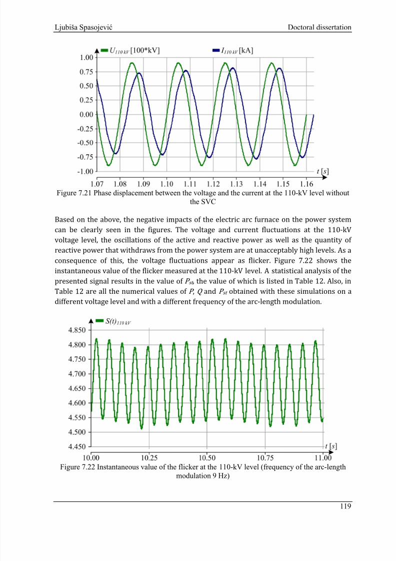
8/12/2019 Voltage fluctuation in industrial network and compensation measures
http://slidepdf.com/reader/full/voltage-fluctuation-in-industrial-network-and-compensation-measures 125/156
Ljubiša Spasojević Doctoral dissertation
Figure 7.21 Phase displacement between the voltage and the current at the 110-kV level without
the SVC
Based on the above, the negative impacts of the electric arc furnace on the power system
can be clearly seen in the figures. The voltage and current fluctuations at the 110-kVvoltage level, the oscillations of the active and reactive power as well as the quantity ofreactive power that withdraws from the power system are at unacceptably high levels. As aconsequence of this, the voltage fluctuations appear as flicker. Figure 7.22 shows the
instantaneous value of the flicker measured at the
110-
kV level. A statistical analysis of the
presented signal results in the value of P st , the value of which is listed in Table 12. Also, inTable 12 are all the numerical values of P , Q and P st obtained with these simulations on a
different voltage level and with a different frequency of the arc-length modulation.
Figure 7.22 Instantaneous value of the flicker at the 110-kV level (frequency of the arc-length
modulation 9 Hz)
119

8/12/2019 Voltage fluctuation in industrial network and compensation measures
http://slidepdf.com/reader/full/voltage-fluctuation-in-industrial-network-and-compensation-measures 126/156

8/12/2019 Voltage fluctuation in industrial network and compensation measures
http://slidepdf.com/reader/full/voltage-fluctuation-in-industrial-network-and-compensation-measures 127/156
Ljubiša Spasojević Doctoral dissertation
Table 14 Simulated values with connected SVC for the period t<6 s at the 35-kV level
With SVC - P controllerArc lengthmodulation
P [MW] Q [MVAr] cosφ P st
5 Hz
Network 110 kV 61.43 5.25 0.99
0.56 Network 35 kV 60.85 ≈ 0 1
Furnace 0.74 kV 56.47 56.43 0.70
9 Hz
Network 110 kV 61.30 5.22 0.99
0.65 Network 35 kV 60.72 ≈ 0 1
Furnace 0.74 kV 56.49 56.15 0.70
11 Hz
Network 110 kV 60.57 7.57 0.99
0.76 Network 35 kV 60.75 2.25 0.99
Furnace 0.74 kV 56.24 56.26 0.70
13 Hz
Network 110 kV 61.09 12.58 0.98
0.96 Network 35 kV 60.50 6.693 0.99
Furnace 0.74 kV 56.09 56.16 0.70
Waveforms of the all simulated signals (frequency of arc-length modulation 9 Hz) are
presented in the figures from 7.23 to 7.28. Figure 7.23 shows the waveforms of the active
and reactive powers measured at the low-voltage level of the furnace transformer. For the
period t <6 s the furnace operates with full load. If we compare Figure 7.23 (t <6 s) andFigure 7.12 we can see that the fluctuations of the active and reactive powers are
approximately the same. Based on this we can conclude that the furnace works at the same
operating point
, i.e.
, the industrial process in the furnace is not changed
, irrespective
whether the SVC is connected or not. At the moment t 6 s, the furnace load is changed.
In Figure 7.24 we can see the positive effects of the operation of the SVC controller. We can
see that the fluctuations of the active and reactive powers at the low-voltage side of the
substation transformer (meddle-level) are significantly reduced compared to thefluctuations of the active and reactive powers that can be seen in Figure 7.13. Also, it isclear that the quantity of the downloaded reactive power from the power system is
practically negligible. At the moment t 6 s, the furnace load is changed. As can be seen in
Figure 7.24, this change of the furnace load does not have any impact on the proper
operation of the controller, i.e., the controller continues to minimize the fluctuations andthe quantity of the downloaded reactive power from the power system also for the period
t >6.
121

8/12/2019 Voltage fluctuation in industrial network and compensation measures
http://slidepdf.com/reader/full/voltage-fluctuation-in-industrial-network-and-compensation-measures 128/156
Ljubiša Spasojević Doctoral dissertation
Figure 7.23 Simulated signals of active and reactive powers with connected SVC at the low-
voltage level of the furnace transformer (frequency of the arc-length modulation 9 Hz)
Figure 7.24 Simulated signals of the active and reactive powers of the furnace with the SVC at
the low-voltage level of the substation transformer before and after the change of furnace load(frequency of the arc-length modulation 9 Hz)
The waveforms of the active and reactive powers at the 110-kV level are presented in
Figure 7.25. It should be noted that there is still downloading of the reactive energies fromthe power system. In fact, it is the reactive energy which is spent for magnetizing the coreof the substation transformer. Although there is a consumption of reactive power the
power factor (cosφ ) is within the prescribed limits, as can be seen in Table 14. In most
cases the minimum allowed value of cosφ is 0.95. If necessary, this quantity of reactiveenergy can also be fully compensated using the proposed controller.
122

8/12/2019 Voltage fluctuation in industrial network and compensation measures
http://slidepdf.com/reader/full/voltage-fluctuation-in-industrial-network-and-compensation-measures 129/156
Ljubiša Spasojević Doctoral dissertation
Figure 7.25 Simulated signals of the active and reactive powers at the 110-kV level downloaded
from the power system with the SVC (frequency of the arc-length modulation 9 Hz)
In Figure 7.26 we can see a waveform of the RMS value of the voltage at the medium-
voltage level. We can see that the fluctuations of the RMS value of the voltage at Figure 7.26
are lower than the fluctuations that can be seen in Figure 7.16 (the case when the
controller does not operate). As a direct consequence of the lower voltage fluctuations,there is lower level of flicker at 110 kV.
Figure 7.26 Fluctuations of RMS voltage at the medium-voltage level with the connected SVC
(frequency of the arc-length modulation 9 Hz)
At
the moment t6
s when the furnace’s load is changed, as a consequence of a decreasedactive power there is a lower value of the current. This lower value of the current means a
123
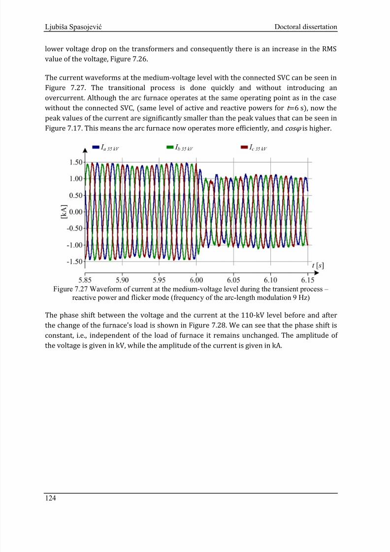
8/12/2019 Voltage fluctuation in industrial network and compensation measures
http://slidepdf.com/reader/full/voltage-fluctuation-in-industrial-network-and-compensation-measures 130/156
Ljubiša Spasojević Doctoral dissertation
lower voltage drop on the transformers and consequently there is an increase in the RMSvalue of the voltage, Figure 7.26.
The current waveforms at the medium-voltage level with the connected SVC can be seen inFigure 7.27. The transitional process is done quickly and without
introducing an
overcurrent. Although the arc furnace operates at the same operating point as in the casewithout the connected SVC, (same level of active and reactive powers for t 6 s), now thepeak values of the current are significantly smaller than the peak values that can be seen inFigure 7.17. This means the arc furnace now operates more efficiently, and cosφ is higher.
Figure 7.27 Waveform of current at the medium-voltage level during the transient process –
reactive power and flicker mode (frequency of the arc-length modulation 9 Hz)
The phase shift between the voltage and the current at the 110-kV level before and after
the change of the furnace's load is shown in Figure 7.28. We can see that the phase shift isconstant, i.e., independent of the load of furnace it remains unchanged. The amplitude of
the voltage is given in kV, while the amplitude of the current is given in kA.
124

8/12/2019 Voltage fluctuation in industrial network and compensation measures
http://slidepdf.com/reader/full/voltage-fluctuation-in-industrial-network-and-compensation-measures 131/156
Ljubiša Spasojević Doctoral dissertation
Figure 7.28 Phase displacement between the voltage and the current at the 110-kV level
(frequency of the arc-length modulation 9 Hz)
The waveforms of the thyristor’s ignition angle can be seen in Figure 7.29.
Figure 7.29 Values of the tyristor's ignition angle, α, the reactive power and the flicker-
regulation mode (frequency of the arc-length modulation 9 Hz)
Furthermore, the figures from Figure 7.30 to Figure 7.32 present the waveforms of the
active and the reactive powers of the SVC device. Here, it should be mentioned that the
direction of the power is defined as being positive when the power flows from the SVCdevice to the arc-furnace transformer (shown in Figure 7.10). As a consequence of that, we
have negative values of the active power of the SVC and TCR. The negative value of the
active power means that the SVC and TCR consume active power fromthe system and it
actually represents the active losses in the SVC device. In Figure 7.30 we can see the total
125
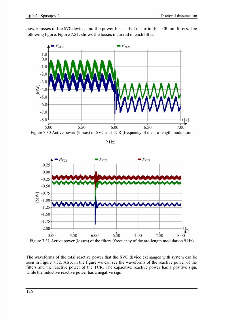
8/12/2019 Voltage fluctuation in industrial network and compensation measures
http://slidepdf.com/reader/full/voltage-fluctuation-in-industrial-network-and-compensation-measures 132/156
Ljubiša Spasojević Doctoral dissertation
power losses of the SVC device, and the power losses that occur in the TCR and filters. Thefollowing figure, Figure 7.31, shows the losses incurred in each filter.
Figure 7.30 Active power (losses) of SVC and TCR (frequency of the arc-length modulation
9 Hz)
Figure 7.31 Active power (losses) of the filters (frequency of the arc-length modulation 9 Hz)
The waveforms of the total reactive power that the SVC device exchanges with system can be
seen in Figure 7.32. Also, in the figure we can see the waveforms of the reactive power of the
filters and the reactive power of the TCR. The capacitive reactive power has a positive sign,
while the inductive reactive power has a negative sign.
126

8/12/2019 Voltage fluctuation in industrial network and compensation measures
http://slidepdf.com/reader/full/voltage-fluctuation-in-industrial-network-and-compensation-measures 133/156
Ljubiša Spasojević Doctoral dissertation
Figure 7.32 Simulated signal of the reactive power of the SVC, TCR and FC (frequency of the
arc-length modulation 9 Hz)
Voltage-regulation mode
Finally, the case when the SVC operates in voltage-regulation mode was simulated. Like in
the mode of reactive power and flicker regulation, f or the period t <6 s the furnace operates
with a full nominal load and at the moment t
6 s the load of the furnace is changed. Figure
7.33 shows the waveforms of active and reactive powers at the medium-voltage level
downloaded from the power system in this case.
Figure 7.33 Simulated signals of the active and reactive powers at the medium-voltage level
downloaded from the power system (frequency of the arc-length modulation 9 Hz)
127

8/12/2019 Voltage fluctuation in industrial network and compensation measures
http://slidepdf.com/reader/full/voltage-fluctuation-in-industrial-network-and-compensation-measures 134/156
Ljubiša Spasojević Doctoral dissertation
At the moment t 6 s the load of the furnace is changed and as a consequence of thisreduced load, there is an increase in the voltage, Figure 7.34. In Figure 7.34 we can see thatthe system reaches the desired value (in this case 1 p.u.) of the voltage after a change of the
load for a short period. If we compare
Figure 7.34 and
Figure 7.26, itis clear that the
fluctuations of the RMS voltage value in both figures are almost the same, i.e., the flickerlevel is almost the same. Based on this it can be concluded that the SVC with this controllerwhen it operates in voltage-regulation mode also has the ability to reduce the level of
flicker.
Figure 7.34 Fluctuations of RMS voltage at the 35-kV level with the connected SVC, voltage
regulation (frequency of the arc-length modulation 9 Hz)
The current waveforms which system draws from power system at the medium-voltage
level with the connected SVC can be seen in Figure 7.35. Also in this case, like in the
reactive-power and flicker-regulation mode, the transitional process is done quickly andwithout an overcurrent occurring.
128

8/12/2019 Voltage fluctuation in industrial network and compensation measures
http://slidepdf.com/reader/full/voltage-fluctuation-in-industrial-network-and-compensation-measures 135/156
Ljubiša Spasojević Doctoral dissertation
Figure 7.35 Waveform of the current which system draws from power system at the medium-
voltage level during the transient process – voltage-regulation mode (frequency of the arc-length
modulation 9 Hz)
The waveforms of the thyristor’s ignition angle can be seen in Figure 7.36.
Figure 7.36 Values of the tyristor's ignition angle α, the voltage-regulation mode (frequency of
the arc-length modulation 9 Hz)
129

8/12/2019 Voltage fluctuation in industrial network and compensation measures
http://slidepdf.com/reader/full/voltage-fluctuation-in-industrial-network-and-compensation-measures 136/156
Ljubiša Spasojević Doctoral dissertation
7.7 Modelling of the electric-arc length using a signal that
involves the all-important frequencies for flicker
As in the previous section, firstly the simulation of the realistic model of the steel factory withoutthe SVC was carried out. All the simulation parameters are unchanged, except the function
which is used for modelling the arc length. Also, the procedure for the simulation is the same.
Frist, simulations without the connected SVC were made. After these simulations, simulations
with the connected SVC were made. During the simulating process with the connected SVC at
the moment t =6 s the furnace’s load is changed.
Simulations without the connected SVC
In Table 15 the numerical values of P, Q and Pst obtained by simulations for the full load withoutthe connected SVC are listed. If we compare the data from Table 15 with the data in Table 12 we
can see that the active and reactive powers and the power factor have approximately the same
values. This means that the furnace works at the same operating point.
Table 15 Simulated values of the active (P) and reactive (Q) powers and
the flicker level (Pst ) without the connected SVC
Without SVC - P controller P [MW] Q [MVAr] cosφ P st
Network 110 kV 58.89 79.28 0.601.55 Network 35 kV 57.68 69.34 0.64
Furnace 0.74 kV 56.07 56.77 0.70
In the next figures are all the signals obtained with these simulations. In Figure 7.37 we can
see the simulated signals of the active and reactive powers at the low-voltage level of thefurnace transformer. Now, we can see that the fluctuations are higher and include morethan one frequency. For this case it can be said that it is more realistic than the case that
includes only one frequency.
130

8/12/2019 Voltage fluctuation in industrial network and compensation measures
http://slidepdf.com/reader/full/voltage-fluctuation-in-industrial-network-and-compensation-measures 137/156
Ljubiša Spasojević Doctoral dissertation
Figure 7.37 Simulated signals of the active and reactive powers without the SVC at the low-
voltage level of the furnace transformer
The simulated signals of the active and reactive powers that the system withdraws from
the power system can be seen in Figure 7.38.
Figure 7.38 Simulated signals of the active and reactive powers without the SVC at the 110-kV
level
The voltage fluctuations at the medium-voltage level can be seen in Figure 7.39, while the
fluctuations of the current which system draws from power system at the same voltage
level are presented in Figure 7.40. The waveform of the RMS voltage value at the medium-
voltage level is shown in Figure 7.41.
131
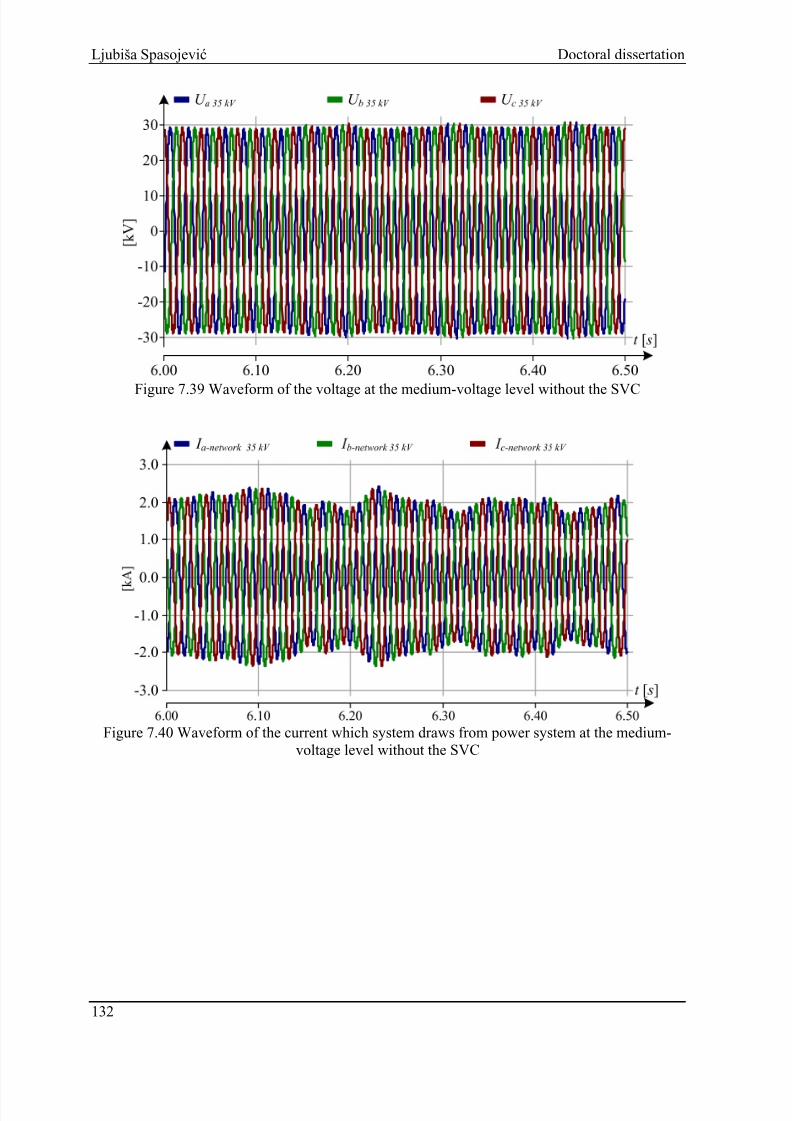
8/12/2019 Voltage fluctuation in industrial network and compensation measures
http://slidepdf.com/reader/full/voltage-fluctuation-in-industrial-network-and-compensation-measures 138/156

8/12/2019 Voltage fluctuation in industrial network and compensation measures
http://slidepdf.com/reader/full/voltage-fluctuation-in-industrial-network-and-compensation-measures 139/156
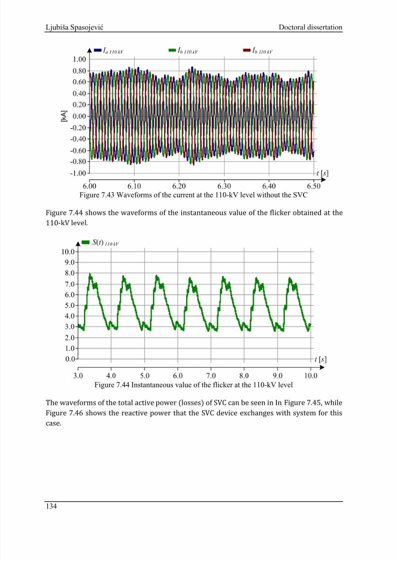
8/12/2019 Voltage fluctuation in industrial network and compensation measures
http://slidepdf.com/reader/full/voltage-fluctuation-in-industrial-network-and-compensation-measures 140/156
Ljubiša Spasojević Doctoral dissertation
Figure 7.43 Waveforms of the current at the 110-kV level without the SVC
Figure 7.44 shows the waveforms of the instantaneous value of the flicker obtained at the110-kV level.
Figure 7.44 Instantaneous value of the flicker at the 110-kV level
The waveforms of the total active power (losses) of SVC can be seen in In Figure 7.45, whileFigure 7.46 shows the reactive power that the SVC device exchanges with system for this
case.
134

8/12/2019 Voltage fluctuation in industrial network and compensation measures
http://slidepdf.com/reader/full/voltage-fluctuation-in-industrial-network-and-compensation-measures 141/156
Ljubiša Spasojević Doctoral dissertation
Figure 7.45 Active power of the TCR and the SVC
Figure 7.46 Reactive power of the FC, the TCR and the SVC
Reactive power and flicker regulation mode
In this section are the results of simulations with the connected SVC. In Table 16 the
numerical values of P , Q, cosφ and P st obtained by simulations for the periods t<6 s and
t>6 s with the connected SVC are listed. At the moment t 6 s, the furnace’s load is changed.
135

8/12/2019 Voltage fluctuation in industrial network and compensation measures
http://slidepdf.com/reader/full/voltage-fluctuation-in-industrial-network-and-compensation-measures 142/156
Ljubiša Spasojević Doctoral dissertation
Table 16 Simulated values with the connected SVC for the period at MV level – reactive power
and flicker-regulation mode
With SVC - P controller t < 6 s t > 6 s
P [MW] Q [MVAr] cosφ P st P [MW] Q [MVAr] cosφ P st Network 110 kV 61.78 5.00 0.99
0.80
49.11 3.35 0.99
0.68 Network 35 kV 61.24 ≈ 0 1 48.77 ≈ 0 0.99
Furnace 0.74 kV 56.03 57.07 0.70 41.60 46.18 0.67
Figure 7.47 shows the simulated signals of the active and reactive powers with theconnected SVC at the low-voltage level of the furnace transformer before and after thechange of the furnace’s load. Like in all the simulations before, the furnace operates at the
same operating point.
Figure 7.47 Simulated signals of the active and reactive powers with the connected SVC at the
low-voltage level of the furnace transformer
In Figure 7.48 we can see the simulated signals of the active and reactive powers with the
SVC atthe low-voltage level of the substation transformer before and after the change of
the furnace’s load. From the figure we can see that the change of the furnace’s load does nothave an influence on the work of the controller. The controller continues to minimize the
fluctuations and the quantity of the downloaded reactive power from the power system, independent of the level of the load.
136
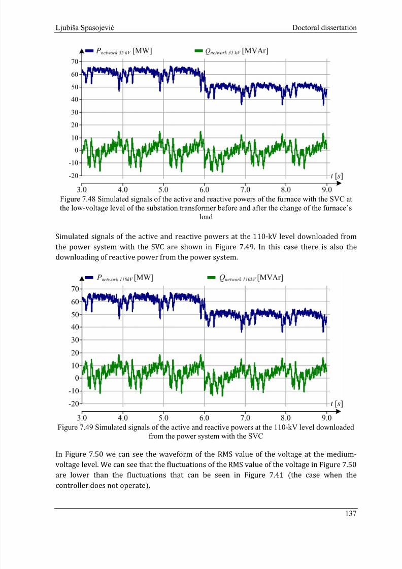
8/12/2019 Voltage fluctuation in industrial network and compensation measures
http://slidepdf.com/reader/full/voltage-fluctuation-in-industrial-network-and-compensation-measures 143/156
Ljubiša Spasojević Doctoral dissertation
Figure 7.48 Simulated signals of the active and reactive powers of the furnace with the SVC at
the low-voltage level of the substation transformer before and after the change of the furnace’s
load
Simulated signals of the active and reactive powers at the 110-kV level downloaded fromthe power system with the SVC are shown in Figure 7.49. In this case there is also the
downloading of reactive power from the power system.
Figure 7.49 Simulated signals of the active and reactive powers at the 110-kV level downloaded
from the power system with the SVC
In Figure 7.50 we can see the waveform of the RMS value of the voltage at the medium-
voltage level. We can see that the fluctuations of the
RMS value of the voltage in
Figure 7.50
are lower than the fluctuations that can be seen in Figure 7.41 (the case when thecontroller does not operate).
137

8/12/2019 Voltage fluctuation in industrial network and compensation measures
http://slidepdf.com/reader/full/voltage-fluctuation-in-industrial-network-and-compensation-measures 144/156
Ljubiša Spasojević Doctoral dissertation
Figure 7.50 Fluctuations of the RMS voltage at the medium-voltage level with the connected
SVC
The waveforms of the currents at the medium-voltage level during the transient process
are presented in Figure 7.51.
Figure 7.51 Waveforms of the currents at the medium-voltage level during the transient process
– reactive power and flicker mode
Figure 7.52 shows the instantaneous value of the flicker at the 110-kV level.
138

8/12/2019 Voltage fluctuation in industrial network and compensation measures
http://slidepdf.com/reader/full/voltage-fluctuation-in-industrial-network-and-compensation-measures 145/156
Ljubiša Spasojević Doctoral dissertation
Figure 7.52 Instantaneous value of the flicker at the 110-kV level
Voltage-regulation mode
In this section are the figures with the waveforms of the signal obtained by simulations in
the voltage-regulation mode. In Figure 7.53 we can see the RMS voltage fluctuations at theMV level. At the moment t 6 s the load of furnace is changed. From Figure 7.53 it is clear
that the controller operates correctly before and after the
furnace’s load is changed.In
Figure 7.54 we can see the waveforms of the currents which system draws from powersystem at MV level and it is clear that the transitional process is done quickly and withoutany overcurrent occurring.
Figure 7.53 Fluctuations of the RMS voltage at the 35-kV level with the connected SVC, voltage
regulation
139

8/12/2019 Voltage fluctuation in industrial network and compensation measures
http://slidepdf.com/reader/full/voltage-fluctuation-in-industrial-network-and-compensation-measures 146/156
Ljubiša Spasojević Doctoral dissertation
Figure 7.54 Waveform of the current which system draws from power system at the medium-
voltage level during the transient process – voltage-regulation mode
Figure 7.55 presents the simulated signals of the active and reactive power (at the low-
voltage level of the substation transformer) downloaded from the power system before
and after the change of the furnace’s load.
Figure 7.55 Simulated signals of the active and reactive powers (medium-voltage level)
downloaded from the power system
In Figure 7.56 we can see the waveform of the tyristor's ignition angle α, before and afterthe furnace’s load.
140

8/12/2019 Voltage fluctuation in industrial network and compensation measures
http://slidepdf.com/reader/full/voltage-fluctuation-in-industrial-network-and-compensation-measures 147/156
Ljubiša Spasojević Doctoral dissertation
Figure 7.56 Values of the thyristor's ignition angle α, voltage-regulation mode
7.8 Simulation with another frequency spectrum
In order to verify the accuracy of the designed controller model, in this section thenumerical results of additional simulations are presented. All the parameters of thesimulation model are unchanged, except for the law of the arc-length variation. The
calculate procedure of the law of the arc-length variation is identical to the procedure
described in Chapter 6. The only difference is that the starting point for the calculation ofthe law of the arc-length is changed, i.e., a different measured signal (signal obtained by
real measurement at other arc furnace location) is taken. According to the previouslydescribed procedure, a representative sample from the measured signal was calculated and
selected. Furthermore, from that representative sample the law of the arc-length wascalculated. Figure 2 shows the waveform of the electric arc length obtained using this
simulation. If we compare Figure 6.22 with Figure 7.57, it is clear that these are two
different arcs with a different frequency spectrum. Also, we can see that the length of arc l 1
is longer than the length of arc l shown in
Figure 7.57.
In Table 17 the numerical values of P, Q, cosφ and P st obtained by simulations for this case
with and without the connected SVC are listed. We can see that the active and reactivepowers and the power factor of the furnace have approximately the same values. This
means that the furnace works at the same operating point. The active power that the
system draws from the power system now is larger. That is a consequence of the existing
losses in the SVC device. In addition, we can see the difference between the power factor
and the level of flicker. With the connected SVC the power factor is almost equal to 1, whilethe
flicker level is lower than 1. Based onthis we can conclude that in this case the
proposed controller also works correctly.
141
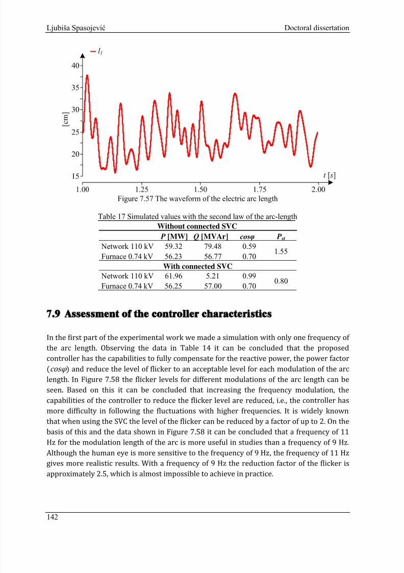
8/12/2019 Voltage fluctuation in industrial network and compensation measures
http://slidepdf.com/reader/full/voltage-fluctuation-in-industrial-network-and-compensation-measures 148/156
Ljubiša Spasojević Doctoral dissertation
Figure 7.57 The waveform of the electric arc length
Table 17 Simulated values with the second law of the arc-length
Without connected SVC P [MW] Q [MVAr] cosφ P st
Network 110 kV 59.32 79.48 0.591.55
Furnace 0.74 kV 56.23 56.77 0.70
With connected SVC
Network 110 kV 61.96 5.21 0.990.80
Furnace 0.74 kV 56.25 57.00 0.70
7.9 Assessment of the controller characteristics
In the first part of the experimental work we made a simulation with only one frequency ofthe arc length. Observing the data in Table 14 it can be concluded that the proposed
controller has the capabilities to fully compensate for the reactive power, the power factor
(cosφ ) and reduce the level of flicker to an acceptable level for each modulation of the arc
length. In
Figure 7.58 the flicker levels for different modulations of the arc length can be
seen. Based on this it can be concluded that increasing the frequency modulation, thecapabilities of the controller to reduce the flicker level are reduced, i.e., the controller has
more difficulty in following the fluctuations with higher frequencies. It is widely knownthat when using the SVC the level of the flicker can be reduced by a factor of up to 2. On the
basis of this and the data shown in Figure 7.58 it can be concluded that a frequency of 11Hz for the modulation length of the arc is more useful in studies than a frequency of 9 Hz.Although the human eye is more sensitive to the frequency of 9 Hz, the frequency of 11 Hz
gives more realistic results. With a frequency of 9 Hz the reduction factor of the flicker is
approximately 2.5,which is almost impossible to achieve in practice.
142

8/12/2019 Voltage fluctuation in industrial network and compensation measures
http://slidepdf.com/reader/full/voltage-fluctuation-in-industrial-network-and-compensation-measures 149/156
Ljubiša Spasojević Doctoral dissertation
Figure 7.58 Simulated values of the flicker level with the connected SVC for different
modulation frequencies (for P furnace≈56.21 MW)
In the second part of the experimental work, the length of the arc is modulated by a signal
that included the full spectrum of characteristic frequencies for the occurrence of the
flicker. Based on the data obtained with these simulations, whose numerical values are
presented in Table 16, we can see that in this case, the controller successfully minimizesthe negative influences of the
EAF on the power system. If wecompare the waveforms
shown in the figures obtained by the simulations when we have only one frequency for themodulation of the arc length with the figures when we have the full spectrum ofcharacteristic frequencies we can see that there is the same trend of behaviour for the
controller. The ability to compensate for the reactive power and voltage control in both
cases can be realized. Only that the compensation of the flicker level for some individualfrequencies is better than in the case if we have the whole spectrum of characteristicfrequencies. Also, we can see that in both cases the transition process in the EAF ( a suddenchange of power) does not affect the stable operation of the controller.In Figure 7.58 we can see the level of flicker with and without the connected SVC device with the first law of the arc-length. The level of flicker with and without the connected SVCdevice with the second law of the arc-length is same as shown in Figure 7.58.
We can see that the correction factor of the level of flicker in both cases is equal to 1.92. Asalready mentioned, using the SVC the level of the flicker can be reduced by a factor of 2.Based on all this, we can conclude that by using the proposed controller we can achieve
practically the maximum efficiency of the SVC, regardless which spectrum produces
electric arc furnace at the connection point. If we compare the pictures 7.58 and 7.59 we
can see that modelling the
electric arc length with a frequency of 11 Hz producesacceptable results for the compensation, i.e., the results obtained in this way are
143

8/12/2019 Voltage fluctuation in industrial network and compensation measures
http://slidepdf.com/reader/full/voltage-fluctuation-in-industrial-network-and-compensation-measures 150/156
Ljubiša Spasojević Doctoral dissertation
approximately the same as the results obtained using simulations that included the wholespectrum of characteristic frequencies. It is important to note that the active power of the
electric arc furnace in all the simulations remains the same.
Figure 7.59 Simulated values of the flicker level with and without the connected SVC; the arc
length modulated with first law of the arc-length to occur
144

8/12/2019 Voltage fluctuation in industrial network and compensation measures
http://slidepdf.com/reader/full/voltage-fluctuation-in-industrial-network-and-compensation-measures 151/156
Ljubiša Spasojević Doctoral dissertation
8 Conclusion
This doctoral dissertation deals with the negative impacts of electric arc furnaces in the
power system. Generally, we know that the EAFs represent large consumers of electrical
energy, which because of their nonlinear characteristics have a strong feedback influenceon the power quality at the electric power system, and as such require the installation ofcompensation devices. In the development and design process of compensating devices an
important role is played by a simulation model of the EAF. The process of developing and
designing the compensation devices for the EAF represents a major problem. In particular, this problem is expressed (because of the non-linear electrical characteristics) when weneed to develop and design the simulation model of the EAF.This dissertation i
s divided into two parts: first isthe theoretical part and second is the
research-development part of the work. The theoretical part includes the first 5 chaptersand presents the existing situation and issues, while the research-development part of this
work is contained in the last three chapters, and in it are the results of the research work
and solutions to some existing problems. Also, the research-development part of the
dissertation includes the contributions to science. The key contributions to science of this
doctoral dissertation are from the fields of the development and the design of the real
model of the EAF and the control algorithm for the compensation device in order to
eliminate the negative impacts of the EAF on the power system.
In this doctoral dissertation a new method for modelling electric arc furnaces based onrepresentative samples of voltages and currents is presented. The proposed arc-furnace
model provides the waveforms of the voltage and current as well as the characteristics(spectrum of interharmonics, flicker level) that are almost equal to the waveforms in thereal plant.
The proposed method is based on a deterministic approach for the generation of the arc
length. The arc-length variation is derived from the measured interharmonic spectrum of
an arc furnace. An advantage of the approach proposed in thisthesis is that it can generate
a full set of frequencies that cause the flicker (i.e., interharmonics) which are generated bythe furnace.
The new model can be used for a comprehensive analysis of the influence of the electric arcfurnace on the network, as it produces similar conditions in the network to the actualfurnace. The proposed model is general and can be used for all arc furnaces. However,furnaces differ substantially, not only due to their different sizes, but also due to thedifferent melting processes, different electrode regulators and different connections to thenetwork. Therefore, for an accurate representation of a particular arc-furnace,measurements are needed for the calibration of the arc-
furnace model. Generally, it would145

8/12/2019 Voltage fluctuation in industrial network and compensation measures
http://slidepdf.com/reader/full/voltage-fluctuation-in-industrial-network-and-compensation-measures 152/156
Ljubiša Spasojević Doctoral dissertation
be possible to group the furnaces based on their effect on the network. This would requirean analysis of a larger number of furnaces and is a goal of our future work.
The simulation results showed that the modelling of an
electric arc length with a frequencyof 11 Hz produces results that are comparable with the results obtained by simulations inthe case when the length of electric arc is modelled with the whole spectrum ofcharacteristic frequencies. The research-development part of this doctoral dissertation relates to the developmentand implementation of an SVC controller. In this part of the doctoral dissertation we
presented a method for developing and implementing an SVC controller in a feedback-loop
strategy. The presented controller is based on the transfer function of the TCRmathematical model, and was designed in the d-q coordinate system. The proposed
controller was designed with the objective being to eliminate the negative impact caused by
electric arc furnaces (EAFs) on a power system.
A mathematical model of the proposed SVC controller in the d-q synchronous rotating
coordinate system (SRCS) was developed first. Then, a completely stability analysis of the
system (analysis in dynamic and steady-state conditions) was carried out. In the end, the
efficiency of the presented controller is demonstrated by means of computer simulations of an
actual steel-factory network model.
The major advantages of the proposed controller are the better flicker compensation, theability to regulate the voltage and the requirement for only single
-point network
measurements. Using an actual industrial network model, the proposed controller wasvalidated by means of simulations. The simulation results showed that the proposed model
can be used successfully to compensate for the reactive power, reduce the flicker level or toregulate the voltage. The main advantages of the proposed controller are good flickercompensation, the ability to regulate the voltage and that its implementation requires onlya single point for the network measurement. A single measurement point also means alower price for the installation of the system and fewer possibilities for failure.
The control algorithm proposed in this thesis
can also be applied to other types of FACTSdevices, such as a STATCOM or thyristor-controlled series compensator. The controlalgorithm was developed for positive system currents. The arc-furnace unbalance will beinvestigated in future work. Also, future work on the subject will include an evaluation ofthe proposed controller in a real-time digital simulator (hardware in the loop).
146
8/12/2019 Voltage fluctuation in industrial network and compensation measures
http://slidepdf.com/reader/full/voltage-fluctuation-in-industrial-network-and-compensation-measures 153/156
Ljubiša Spasojević Doctoral dissertation
9 References
[1] Standard SIST EN 50160:2011: Voltage characteristics of electricity supplied by public
electricity networks.
[2] Standard SIST EN 61000–4–30:2003: EMC Part 4, Section 30 – Testing and
measurement techniques – Power quality measurement methods.
[3] M. Maksić, I. Papič, Calculating flicker propagation in a meshed high voltage networkwith interharmonics and representative voltage samples, Electrical Power and Energy
Systems 42 (2012) 179–187.
[4] “Flicker Measurement and Evaluation”, UIE publication, 1992
[5] IEC 61000–3–3, Edition 1.1: “Electromagnetic compatibility (EMC) – Part 3–3: Limits –
Limitation of voltage changes, voltage fluctuations and flicker in References 168 public
low–voltage supply systems, for equipment with rated current <= 16 A per phase and not
subject to conditional connection”.
[6] IEC/TR 61000–4–15 Standard, EMV – Testing and measuring techniques, Flickermeter –
Functional and design specifications.
[7] IEEE standard 141 – 1993: “IEEE recommended practice for electric power distribution
for industrial plants”, 1993.
[8]
Cai R.: Flicker Interaction Studies and Flickermeter Improvement, doctoral dissertation,Technische Universiteit Eindhoven, 2009.
[9] S. Mendis, M. Bishop, and J. Witte. “Investigations of Voltage Flicker in Electric Arc
Furnace Power Systems”. IEEE Industry Applications Magazine, Jan./ Febr. 1996.
[10] P. Ashmole. “Quality of Supply-voltage fluctuations - part 2”. Power Engineering
Journal, Apr. 2001.
[11] Z. Zhang, N. Fahmi and W. Norris. “Flicker Analysis and Methods for Electric Arc
Furnace Flicker Mitigation (A Survey)”. 2001 IEEE Porto Power Tech Conference,Porto, Portugal, Sept. 2001
[12] T. Thiringer, T. Petru and S. Lundberg. “Flicker contribution from wind turbineinstallations”, IEEE Trans. Energy Conv. vol. 17, pp. 114–118, Mar. 2002.
[13] J. Tande and K. Uhlen. ”Wind Turbines in Weak Grids – Constraints and Solutions”.
16th Int. Conf. On Electricity Distribution, CIRED 2001, June 2001.
[14]
Ĺ. Larsson. “Flicker Emission of Wind Turbines during Continuous Operation”. IEEETrans. Energy Conv. vol. 17, pp. 114-118, Mar. 2002
147
8/12/2019 Voltage fluctuation in industrial network and compensation measures
http://slidepdf.com/reader/full/voltage-fluctuation-in-industrial-network-and-compensation-measures 154/156
Ljubiša Spasojević Doctoral dissertation
[15] Ĺ. Larsson. “Flicker Emission of Wind Turbines during Continuous Operation”. IEEE
Trans. Energy Conv. vol. 17, pp. 114-118, Mar. 2002.
[16] M. Maksić, Calculating flicker propagation in a meshed high voltage network withinterharmonics and representative voltage samples, doctoral dissertation, Faculty of
Electrical Engineering, University Ljubljana 2011
[17] A. Baggini, Handbook of Power Quality, Wiley, June 16, 2008
[18] H. Andrei1, C. Cepisca, S. Grigorescu, Power Quality and Electrical Arc Furnaces,
Politehnica University of Bucharest, Romania
[19] J. Voršič, J. Bratina, Electrotermija, Univerza v Mariboru, Maribor 2000
[20] Y. Yang, Y. Xiao and M.A. Reuter, Analysis of transport phenomena in submerged arc
furnace for ferrochrome production, Delft University of Technology, Dept. of Applied
Earth Sciences Mijnbouwstraat 120, 2628 RX Delft, The Netherlands. [21] A. H. Howatson, An Introduction to Gas Discharges, Pergamon Press, Oxford
[22] R. M. Mathur, R. K. Varma, Thyristor-based FACTS controllers for electrical
transmission systems, ISBN 0-471-20643-1, 2002
[23] D. Lagator: Kontrola napona i jalove snage, seminarski rad, sveučilište Osjek 2011
[24] N. G. Hingorani, L. Gyugyi, “Understanding FACTS concepts and technology of flexible
AC transmission systems, ISBN 0-7803-3455-8, 1999
[25] Tang, L., Kolluri S., McGrangghan, M. F.: “Voltage flicker prediction for two
simultaneously operated ac arc furnaces”, IEEE Trans. Power Delivery, Vol. 12, No. 2,
1997.
[26] Montanari, G. C., Loggini, M., Cavallini, A., Pitti, L., Zaninelli, D.: “Arc-furnace model
for the study of flicker compensation in electrical networks”, IEEE Trans. Power
Delivery, Vol. 9, No. 4, 1994.
[27] Varadan, S., Makram, E. B., Girgis, A. A.: “A new time domain voltage source model for
an arc furnace EMPT”, IEEE Trans. Power Delivery. Vol. 11, No. 3, 1996
[28] Mayordomo, J. G., Asensi R.: “A Frequency Domain Arc Furnace Model For Harmonic
Power Flows Under Balanced Conditions”, Proceedings of the IEEE 7th International
Conference on Harmonics and Quality of Power, Las Vegas, pp. 419-27, 16-18 Oct.
1996.
[29] Mayordomo, J. G., Beites, L. F., Asensi, R., Izzeddine, M., Zabala, L., Amantegui, J.: ‘A
new frequency domain arc furnace model for iterative harmonic analysis’, IEEE Trans.
Power Delivery, Vol. 12, No. 4, 1997.
148

8/12/2019 Voltage fluctuation in industrial network and compensation measures
http://slidepdf.com/reader/full/voltage-fluctuation-in-industrial-network-and-compensation-measures 155/156
Ljubiša Spasojević Doctoral dissertation
[30] Ozgun, O., Abur, A.: ‘Development of an arc furnace model for power quality studies’,
Power Engineering Society Summer Meeting, IEEE Vol. 1, pp. 507 – 511, 18-22 July
1999.
[31] Ozgun O., Abur A.: ‘Flicker study using a novel arc furnace model’, IEEE Trans. Power
Delivery, Vol. 17, No. 4, 2002.
[32] Zhang L., Liu Y., Ingram M. R., Bradshaw D. T., Eckroad S., Crow M. L.: ‘EAF Voltage
Flicker Mitigation By FACTS/ ESS’, Power System Conference & Exposition, Vol. 1,
pp. 372-378, Oct. 2004.
[33] O’Neill-Carrillo, E., Heydt, G.T., Kostelich, E.J., Venkata, S.S., Sundaram, A.:
‘Nonlinear deterministic modelling of highly varying loads’, IEEE Trans. Power
Delivery, Vol. 14, No. 5, 1999.
[34] Ozgun, O., Abur, A.: ‘Flicker study using a novel arc furnace model’, IEEE Trans.
Power Delivery, Vol. 17, No. 4, 2002.
[35] Maksić, M., Papič, I.: ’Analysis of flicker propagation with representative samples ofnetwork voltage’, IEEE Trans. Power Delivery, Vol. 26, No. 3, 2011.
[36] Maksić, M., Papič, I.: ‘Calculating flicker propagation in a meshed high voltage networkwith interharmonics and representative voltage samples’, Electrical Power and Energy
Systems, Vol. 42, 2011.
[37] Chang, G. W., Chen, C. I. A.: ‘A Comparative Study of Voltage Flicker Envelope
Estimation Methods’, Conference Publications IEEE, pp. 1-6, 20-24 July 2008.
[38] IEEE 1453-2004: ‘Recommended Practice for Measurement and Limits of Voltage
Fluctuations and Associated Light Flicker on AC Power Systems’, 2005.
[39] H. Samet, M.E. Hamedani Golshan, “A wide nonlinear analysis of reactive power time
series related to electric arc furnaces”, Electrical Power and Energy Systems 36, 127-134,
2012.
[40] J. Wang, C. Fu, Y. Zhang, “SVC Control System Based on Instantaneous Reactive Power
Theory and Fuzzy PID”, IEEE Trans. Industrial Electronics, Vol. 55, No. 4, April 2008.
[41] Q. Zhao, J. Jiang, “Robust SVC controller design for improving power system damping”,
IEEE Trans. Power Systems, Vol. 10. No. 4, 1995.
[42] M. C. Lima, H. Tyll, “An overview of static Var compensators technology evolution on a
Brazilian generation and transmission utility”, Proc. IEEE 10th Int. Conf. Harmonics
Quality Power, Vol. 2, pp. 601–606. 6–9 Oct. 2002.
149
8/12/2019 Voltage fluctuation in industrial network and compensation measures
http://slidepdf.com/reader/full/voltage-fluctuation-in-industrial-network-and-compensation-measures 156/156
Ljubiša Spasojević Doctoral dissertation
[43] A. F. Zobaa, M. A. Jovanović, “A comprehensive overview on reactive powercompensation technologies for wind power applications”, Proc. IEEE 12th Int. Power
Electron. Motion Control Conf., pp. 1848–1852. Aug. 2006.
[44] H. Samet, M. Parniani, “Predictive method for improving SVC speed in electric arc
furnace compensation”, IEEE Trans. Power Del., Vol. 22, No. 1, pp. 732–734, Jan. 2007.
[45] M. Noroozian, M. Ghandhari, G. Andersson, “A robust control strategy for shunt and
series reactive compensators to damp electromechanical oscillations”, IEEE Trans.
Power Delivery, Vol. 16, No. 4, 2001.
[46] C. Cheng, Y. Y. Hsu. “Damping of generator oscillations using an adaptive static VAr
compensator”, IEEE Trans.Power Systems, Vol. 7, No. 2, 1992.
[47]
X. Du, L. Peng, L. Zhou. “A hybrid reactive power compensation system consisting ofmulti capacitor banks and a SVG”, Power System Technology, Vol. 32, No. 14, 2008.
[48] E. H. Mamdani, “Application of fuzzy algorithm for control of simple dynamic plant”,
Procedings of IEEE, 121(12): 1585 – 1588. 1974
[49] T. Abdelazim, O. P. Malik, “Intelligent SVC control for transient stability enhancement”,
IEEE Power Engineering Society General Meeting. New York: IEEE, 1701 – 1707.
2005.
C.J. Wu, T.H. Fu, “Effective voltage flicker calculation algorithm using indirect