vol2 chap 3 stormwater hydrology
TRANSCRIPT

8/11/2019 Vol2 Chap 3 Stormwater Hydrology
http://slidepdf.com/reader/full/vol2-chap-3-stormwater-hydrology 1/76
..CHAPTER ..
3
Volume 2 (Technical Guidance) Page 3-1
STORMWATER HYDROLOGY3.1 Introduction to Hydrologic MethodsHydrology is the science dealing with the characteristics, distribution, and movement of water onand below the earth's surface and in the atmosphere. Hydrology in this manual shall be limited toestimating flow peaks, volumes, and time distributions of stormwater runoff. The analysis of theseparameters is fundamental to the design of stormwater management facilities, such as stormdrainage systems and structural stormwater BMPs. In the hydrologic analysis of a developmentsite, there are a number of variable factors that affect the nature of stormwater runoff from the site.Some of the factors that need to be considered include:
• rainfall amount and storm distribution;
• drainage area size, shape and orientation;• ground cover and soil type;
• slopes of terrain and stream channel(s);
• antecedent moisture condition;
• storage potential (floodplains, ponds, wetlands, reservoirs, channels, etc.);
• watershed development potential; and
• characteristics of the local drainage system.
There are a number of empirical hydrologic methods that can be used to estimate runoffcharacteristics for a site or drainage subbasin; however, the following methods presented in thischapter have been selected to support hydrologic site analysis for the design methods andprocedures included in the Manual:
• Rational Method;
• United States Geological Survey (USGS) and Tennessee Valley Authority (TVA) RegressionEquations;
• Soil Conservation Service (SCS) Unit Hydrograph Method;
• Clark Unit Hydrograph;
• Water Quality Volume (WQv) Calculation; and
• Water Balance Calculations.These methods were selected based upon their accuracy in duplicating local hydrologic estimatesfor a range of design storms and the availability of equations, nomographs, and computerprograms to support them.
Table 3-1 lists the hydrologic methods and the circumstances for their use in various analysis anddesign applications. Table 3-2 provides some limitations on the use of several methods.

8/11/2019 Vol2 Chap 3 Stormwater Hydrology
http://slidepdf.com/reader/full/vol2-chap-3-stormwater-hydrology 2/76

8/11/2019 Vol2 Chap 3 Stormwater Hydrology
http://slidepdf.com/reader/full/vol2-chap-3-stormwater-hydrology 3/76
Knox County Tennessee Stormwater Management Manual
Volume 2 (Technical Guidance) Page 3-3
In general:
• the Rational Method is recommended for small, highly impervious drainage areas such asparking lots and roadways draining into inlets and gutters; and
• the USGS regression equations are recommended for drainage areas with characteristicswithin the ranges given for the equations. The USGS equations should be used with cautionwhen there are significant storage areas within the drainage basin or where other drainagecharacteristics indicate that general regression equations might not be appropriate; and
• the TVA regression equations are used for stormwater system design (discussed in Chapter 7),choosing the more conservative solution from between the results of the applicable USGSregression equation and the TVA regression equation.
Note: Users must realize that any hydrologic analysis is only an approximation. The relationshipbetween the amount of precipitation on a drainage basin and the amount of runoff from the basin iscomplex and too little data are available on the factors influencing the rainfall-runoff relationship toexpect exact solutions.
3.1.1 Symbols and Definitions
To provide consistency within this section, the symbols listed in Table 3-3 will be used. Thesesymbols were selected because of their wide use in technical publications. In some cases, thesame symbol is used in existing publications for more than one definition. Where this occurs in thismanual, the symbol will be defined where it occurs in the text or equations.
Table 3-3. Symbols and Definitions for Stormwater RunoffSymbol Definition Units
A Drainage area acres (or mi 2)Bf Baseflow cfsC Runoff coefficient -C f Frequency factor -
CN SCS-runoff curve number -CPv Channel protection volume acre-feet
d Time interval hoursE Evaporation ftE t Evapotranspiration ftFp Pond and swamp adjustment factor -Gh Hydraulic gradient ft/ft
I or i Runoff intensity in/hrIA Percent of impervious cover %I Infiltration ftI Inflows cfs
Ia Initial abstraction from total rainfall inkh Infiltration rate ft/dayL Flow length ftn Manning roughness coefficient (Manning’s “n”) -O f Overflow acre-feetO Outflows cfsP Accumulated rainfall inP 2 2-year, 24-hour rainfall inP w Wetted perimeter ftPF Peaking factor -
8/11/2019 Vol2 Chap 3 Stormwater Hydrology
http://slidepdf.com/reader/full/vol2-chap-3-stormwater-hydrology 4/76
Knox County Tennessee Stormwater Management Manual
Volume 2 (Technical Guidance) Page 3-4
Symbol Definition Units
Q Rate of runoff or depth of runoff cfs or inchesQp Peak rate of discharge cfsQp 2 2-year event peak discharge cfs
Qp 10 10-year event peak discharge cfsQp 25 25-year event peak discharge cfsQp 100 100-year event peak discharge cfsQwq Water quality peak discharge cfsQwv Water quality runoff peak volume in
q Storm runoff during a time interval inqu Unit peak discharge cfs (or cfs/mi 2 /inch)R Clark watershed storage constant -R Hydraulic radius ftRo Runoff acre-feetRv Runoff coefficient -S Ground slope ft/ft or %S Potential maximum retention inS Slope of hydraulic grade line ft/ftTL Lag time hoursTp Time to peak hours
Tt or t t Travel time min or hourst Time min
Tc or t c Time of concentration minTIA Total impervious area %V Velocity ft/sV Pond volume acre-feet
WQv Water quality volume acre-feet
Ws Average ground surface slope as a percentage %
3.1.2 Rainfall Estimation
The first step in any hydrologic analysis is an estimation of the rainfall that will fall on the site for agiven time period. The amount of rainfall can be quantified with the following characteristics:
Duration (hours) – Length of time over which rainfall (storm event) occurs;
Depth (inches) – Total amount of rainfall occurring during the storm duration; and
Intensity (inches per hour) – Rate of rainfall or depth divided by the duration
The frequency of a rainfall event is the recurrence interval of storms having the same duration andvolume (depth). This can be expressed either in terms of exceedance probability or return period .
Exceedance Probability – Probability that a storm event having the specified duration andvolume will be exceeded in one given time period, typically 1-year.
Return Period – Average length of time between events that have the same duration andvolume.
Thus, if a storm event with a specified duration and volume has a 1% chance of occurring in anygiven year, then it has an exceedance probability of 0.01 and a return period of 100-years. Adesign storm event over 24-hours with a 1% chance of occurring in any given year is often referredto as the 100-year, 24-hour storm. This design storm would be developed based on assumptionsregarding intensity and distribution of the storm over the specified timeframe (24-hours for this

8/11/2019 Vol2 Chap 3 Stormwater Hydrology
http://slidepdf.com/reader/full/vol2-chap-3-stormwater-hydrology 5/76
Knox County Tennessee Stormwater Management Manual
Volume 2 (Technical Guidance) Page 3-5
scenario). Therefore, a design storm event is used to estimate actual storm events even though itwould be very unlikely that an actual storm event would match up with all of the design storm eventassumptions.
Rainfall intensities for Knox County are provided in Table 3-4 and should be used for all hydrologicanalysis. The sources of the values in this table are the Weather Bureau Technical Papers TP-25and TP-40 (Hershfield, 1961) and National Weather Service publication Hydro-35 (NOAA, 1977).The intensity values have been adjusted to produce smooth intensity-duration-frequency (IDF)curves and cumulative rainfall distributions. Table 3-5 shows the rainfall depths for hypotheticalstorm events.
Figure 3-1 shows the IDF curves for Knox County for the 1, 2, 5, 10, 25, and 100-year, 24-hourstorms. These curves are plots of the tabular values. No values are given for times less than 5minutes.
Table 3-4. Intensity-Duration-Frequency Curve Data(Sources: Hershfield, 1961; NOAA, 1977)
ARI1 (years) 24-Hour Precipitation Frequency Estimates (inches/hour) by ReturnPeriods
Hours Minutes 2-year 5-year 10-year 25-year 50-year 100-year0.083 5 4.60 5.55 6.25 7.30 7.90 8.600.170 10 3.70 4.60 5.25 6.20 6.80 7.490.250 15 3.19 3.98 4.60 5.45 6.00 6.600.330 20 2.82 3.50 4.10 4.90 5.45 6.020.420 25 2.48 3.12 3.70 4.45 4.95 5.500.500 30 2.22 2.80 3.34 4.03 4.53 5.03
0.580 35 2.02 2.55 3.06 3.67 4.14 4.620.670 40 1.86 2.35 2.82 3.38 3.80 4.240.750 45 1.73 2.18 2.62 3.14 3.53 3.930.830 50 1.62 2.04 2.46 2.94 3.30 3.670.920 55 1.53 1.92 2.32 2.77 3.10 3.451.000 60 1.45 1.82 2.20 2.62 2.93 3.26
1.500 90 1.06 1.36 1.64 1.95 2.18 2.452.000 120 0.86 1.09 1.31 1.55 1.71 1.953.000 180 0.66 0.80 0.97 1.13 1.23 1.386.000 360 0.41 0.50 0.58 0.66 0.75 0.83
12.000 720 0.24 0.30 0.34 0.39 0.43 0.4824.000 1440 0.14 0.17 0.20 0.23 0.25 0.27
1 - ARI= Average Recurrence Interval
Table 3-5. Rainfall Depths for Hypothetical Storm Events
Rainfall Depths for Hypothetical Storm EventsStorm Event 24-Hr Depth (in)
1-year 2.52-year 3.35-year 4.1
10-year 4.825-year 5.5
100-year 6.5

8/11/2019 Vol2 Chap 3 Stormwater Hydrology
http://slidepdf.com/reader/full/vol2-chap-3-stormwater-hydrology 6/76
V ol um
e2
( T e c h n
i c al G
ui d
an
c e )
P a g e 3 - 6
Figure 3-1. Intensity-Duration-Frequency-(IDF) Curves for Knox County 24-hour Storms(Based upon partial duration-based point precipitation frequency estimates for average recurrence intervals (T))
T = 2 - y e a r
T = 5 - y e a r
T = 1 0 - y e a r
T = 2 5 - y e a r
T = 5 0 - y e a r
T = 1 0 0 - y e a r
0
1
2
3
4
5
6
7
8
9
10
0 20 40 60 80
Duration (T c) - Minutes
P r e c i p i t a t i o n D
e p t h ( i n c h e s )

8/11/2019 Vol2 Chap 3 Stormwater Hydrology
http://slidepdf.com/reader/full/vol2-chap-3-stormwater-hydrology 7/76
Knox County Tennessee Stormwater Management Manual
Volume 2 (Technical Guidance) Page 3-7
CIAQ =
3.1.3 Rational Method
A popular approach for determining the peak runoff rate is the Rational Formula. The RationalMethod considers the entire drainage area as a single unit and estimates the peak discharge at themost downstream point of that area.
The Rational Formula follows the assumptions that:
• the rainfall is uniformly distributed of the entire drainage area and is constant over time;
• the predicted peak discharge has the same probability of occurrence (return period) as theused rainfall intensity (I);
• peak runoff rate can be represented by the rainfall intensity averaged over the same timeperiod as the drainage area’s time of concentration (tc); and
• the runoff coefficient (C) is constant during the storm event.
When using the Rational Method some precautions should be considered:
• in determining the C value (runoff coefficient based on land use) for the drainage area,hydrologic analysis should take into account any future changes in land use that might occurduring the service life of the proposed facility;
• if the distribution of land uses within the drainage basin will affect the results of hydrologicanalysis (e.g., if the impervious areas are segregated from the pervious areas), the basinshould be divided into sub-drainage basins. The single equation used for the Rational Methoduses one composite C and one t c value for the entire drainage area; and ,
• the charts, graphs, and tables included in this section are given to assist the engineer inapplying the Rational Method. The engineer shall use sound engineering judgment in applyingthese design aids and shall make appropriate adjustments when specific site characteristicsdictate that these adjustments are appropriate.
3.1.3.1 Application
The Rational Method can be used to estimate stormwater runoff peak flows for the design of gutterflows, drainage inlets, storm drain pipe, culverts and small ditches. It is most applicable to small,highly impervious areas. Knox County policies regarding the use of the Rational Method are asfollows:
• In Knox County, the Rational Method shall not be utilized for drainage areas less than five (5)acres.
• The Rational Method shall not be used for storage design or any other application where amore detailed routing procedure is required.
• The Rational Method shall not be used for calculating peak flows downstream of bridges,culverts or storm sewers that may act as restrictions and impact the peak rate of discharge.
3.1.3.2 EquationsThe Rational Method estimates the peak rate of runoff at a specific watershed location as afunction of the drainage area, runoff coefficient, and mean rainfall intensity for a duration equal tothe time of concentration, t c. The t c is the time required for water to flow from the most remote pointof the basin to the location being analyzed.
The Rational Method is expressed in Equation 3-1. Further explanation of each variable in theRational Method equation is presented in Sections 3.1.3.3 and 3.1.3.4.
Equation 3-1

8/11/2019 Vol2 Chap 3 Stormwater Hydrology
http://slidepdf.com/reader/full/vol2-chap-3-stormwater-hydrology 8/76
Knox County Tennessee Stormwater Management Manual
Volume 2 (Technical Guidance) Page 3-8
where:Q = maximum rate of runoff (cfs)C = runoff coefficient representing a ratio of runoff to rainfallI = average rainfall intensity for a duration equal to the t c (in/hr)
A = drainage area contributing to the design location (acres)
3.1.3.3 Runoff Coefficient
The runoff coefficient (C) is the variable of the Rational Method least susceptible to precisedetermination and requires judgment and understanding on the part of the design engineer. Whileengineering judgment will always be required in the selection of runoff coefficients, typicalcoefficients represent the integrated effects of many drainage basin parameters. Table 3-6 givesthe recommended runoff coefficients for the Rational Method.
It is often desirable to develop a composite runoff coefficient based on the percentage of differenttypes of surfaces in the drainage areas. Composites can be made with the values from Table 3-6by using percentages of different land uses. In addition, more detailed composites can be madewith coefficients for different surface types such as rooftops, asphalt, and concrete. The compositeprocedure can be applied to an entire drainage area or to typical “sample" blocks as a guide to theselection of reasonable values of the coefficient for an entire area.
It should be remembered that the Rational Method assumes that all land uses within a drainagearea are uniformly distributed throughout the area. If it is important to locate a specific land usewithin the drainage area, then another hydrologic method should be used where hydrographs canbe generated and routed through the drainage system.
Using only the impervious area from a highly impervious site (and the corresponding high C factorand shorter time of concentration) can in some cases yield a higher peak runoff value than by usingthe whole site. Peak flow calculations can be underestimated due to areas where the overlandportion of flow is grassy (yielding a longer t c).
Note that the coefficients given in Table 3-6 are applicable for storms of 5 to 10-year frequencies.Less frequent, higher intensity storms may require modification of the coefficient becauseinfiltration and other losses have a proportionally smaller effect on runoff (Wright - McLaughlin
Engineers, 1969). The adjustment of the Rational Method for use with major storms can be madeby multiplying the right side of the Rational Formula by a frequency factor Cf. The RationalFormula for major storm events now becomes:
Equation 3-2 CIAC Q f =
C f values are listed in Table 3-7. The product of C f times C shall not exceed 1.0.
3.1.3.4 Rainfall Intensity (I)The rainfall intensity (I) is the average rainfall rate in in/hr for a selected return period that is basedon a duration equal to the time of concentration (t c). Once a particular return period has beenselected for design and a time of concentration has been calculated for the drainage area, therainfall intensity can be determined from rainfall-intensity-duration data given in Table 3-4 or Figure3-1. Calculation of t c is discussed in detail in the next section.

8/11/2019 Vol2 Chap 3 Stormwater Hydrology
http://slidepdf.com/reader/full/vol2-chap-3-stormwater-hydrology 9/76
V ol um
e2
( T e c h ni c al G
ui d
an
c e )
P a g e 3 - 9
Table 3-6. Recommended Runoff Coefficient Values for Rational MethodRunoff Coefficient (C) by Hydrologic Soil Group and Ground Slope
A B C Land Use
<2% 2 - 6% >6% <2% 2 - 6% >6% <2% 2 - 6% >6% <2%
Forest 0.08 0.11 0.14 0.10 0.14 0.18 0.12 0.16 0.20 0.15
Meadow 0.14 0.22 0.30 0.20 0.28 0.37 0.26 0.35 0.44 0.30
Pasture 0.15 0.25 0.37 0.23 0.34 0.45 0.30 0.42 0.52 0.37
Farmland 0.14 0.18 0.22 0.16 0.21 0.28 0.20 0.25 0.34 0.24
Res. 1 acre 0.22 0.26 0.29 0.24 0.28 0.34 0.28 0.32 0.40 0.31
Res. 1/2 acre 0.25 0.29 0.32 0.28 0.32 0.36 0.31 0.35 0.42 0.34
Res. 1/3 acre 0.28 0.32 0.35 0.30 0.35 0.39 0.33 0.38 0.45 0.36
Res. 1/4 acre 0.30 0.34 0.37 0.33 0.37 0.42 0.36 0.40 0.47 0.38
Res. 1/8 acre 0.33 0.37 0.40 0.35 0.39 0.44 0.38 0.42 0.49 0.41
Industrial 0.85 0.85 0.86 0.85 0.86 0.86 0.86 0.86 0.87 0.86
Commercial 0.88 0.88 0.89 0.89 0.89 0.89 0.89 0.89 0.90 0.89
Streets: ROW 0.76 0.77 0.79 0.80 0.82 0.84 0.84 0.85 0.89 0.89
Parking 0.95 0.96 0.97 0.95 0.96 0.97 0.95 0.96 0.97 0.95
Disturbed Area 0.65 0.67 0.69 0.66 0.68 0.70 0.68 0.70 0.72 0.69

8/11/2019 Vol2 Chap 3 Stormwater Hydrology
http://slidepdf.com/reader/full/vol2-chap-3-stormwater-hydrology 10/76
Knox County Tennessee Stormwater Management Manual
Volume 2 (Technical Guidance) Page 3-10
Table 3-7. Frequency Factors for Rational FormulaRecurrence Interval (years) C f
10 or less 1.025 1.150 1.2
100 1.25
3.1.3.5 Time of Concentration
Use of the Rational Method requires calculating the time of concentration (t c) for each design pointwithin the drainage basin. The duration of rainfall is then set equal to the time of concentration andis used to estimate the design average rainfall intensity (I). The basin time of concentration isdefined as the time required for water to flow from the most remote part of the drainage area to thepoint of interest for discharge calculations. The time of concentration is computed as a summationof travel times within each flow path as follows:
Equation 3-3 tmt t c t t t t ++= 21
here:tc = time of concentration (hours)tt = travel time of segment (hours)m = number of flow segments
Knox County policies regarding the calculation of t c are as follows:
• The t c shall be the longest sub-basin travel time when all flow paths are considered.
• The minimum t c for all computations shall be five (5) minutes.
Time of concentration calculations are subject to the following limitations:
1. the equations presented in this section should not be used for sheet flow on impervious landuses where the flow length is longer than 50 feet; and
2. in watersheds with storm sewers, use care to identify the appropriate hydraulic flow path toestimate t c.
Two common errors should be avoided when calculating time of concentration. First, in somecases runoff from a highly impervious portion of a drainage area may result in a greater peakdischarge than the calculated peak discharge for the entire area. Second, the designer shouldconsider that the overland flow path does not necessarily remain the same when comparing pre-development and post-development areas. Grading operations and development can alter theoverland flow path and length. Selecting overland flow paths for impervious areas that are greaterthan 50 feet should be done only after careful consideration. For typical urban areas, the time ofconcentration consists of multiple flow paths including overland flow, shallow concentrated flow andthe travel time in the storm drain, paved gutter, roadside ditch, or drainage channel.
Overland Flow: Overland flow in urbanized basins occurs from the backs of lots to the street, across and withinparking lots and grass belts, and within park areas, and is characterized as shallow, steady anduniform flow with minor infiltration effects. The travel time (T t) for overland flow over plane surfacesfor distances of less than 300 lineal feet (100 feet for paved surfaces) can be calculated usingManning's kinematic solution (Overton and Meadows, 1976), shown in Equation 3-4. Following theequation, Table 3-8 presents Manning’s “n” roughness coefficients for use in Equation 3-4.

8/11/2019 Vol2 Chap 3 Stormwater Hydrology
http://slidepdf.com/reader/full/vol2-chap-3-stormwater-hydrology 11/76
Knox County Tennessee Stormwater Management Manual
Volume 2 (Technical Guidance) Page 3-11
Equation 3-4( )
( ) 4.05.02
8.0007.0
S P
nLT t =
where:Tt = travel time (hours)
n = Manning's roughness coefficient (see Table 3-8)L = flow length (ft)P 2 = 2-year 24-hour rainfall (inches)S = ground slope, (ft/ft)
Table 3-8. Roughness coefficients (Manning's “n”) 1 (Soil Conservation Service, 1986)
Surface Description n
Smooth surfaces (concrete, asphalt, gravel or bare soil) 0.011Fallow (no residue) 0.05Cultivated soils:
Residue cover 20% 0.06
Residue cover > 20% 0.17Grass:
Short grass prairie 0.15Dense grasses 2 0.24Bermuda grass 0.41
Range (natural) 0.13Woods 3:
Light underbrush 0.40Dense underbrush 0.80
1 The n values are a composite of information by Engman (1986).2 Includes species such as weeping lovegrass, bluegrass, buffalo grass, blue grama grass,and native grass mixtures.3 When selecting n, consider cover to a height of about 0.1 ft. This is the only part of the
plant cover that will obstruct sheet flow.
Additionally, the SCS lag equation is an acceptable method for calculating the time of concentrationfor overland flow (T c) based on watershed lag time (T L). T L is defined as the time between thecenter of mass of excess rainfall to the time of peak runoff (similar to an average flow time for asmall homogeneous area). The following equations can be used to determine T c:
Equation 3-5 Lc T T 67.1=
where:TC = time of concentration of overland flow portion of flow path (hours)TL = NRCS lag time (hours)
Equation 3-6 5.0
7.08.0
1900)1(
s
LW
S LT +=
where:TL = SCS lag time (hours)L = flow length for sheet flow over the surface (feet)S = potential maximum soil retention (inches) = 1000/CN-10Ws = average ground surface slope as a percentage (%)

8/11/2019 Vol2 Chap 3 Stormwater Hydrology
http://slidepdf.com/reader/full/vol2-chap-3-stormwater-hydrology 12/76
Knox County Tennessee Stormwater Management Manual
Volume 2 (Technical Guidance) Page 3-12
Figure 3-2. Average Velocities - Shallow Concentrated Flow(Source: Soil Conservation Service, 1986)

8/11/2019 Vol2 Chap 3 Stormwater Hydrology
http://slidepdf.com/reader/full/vol2-chap-3-stormwater-hydrology 13/76
Knox County Tennessee Stormwater Management Manual
Volume 2 (Technical Guidance) Page 3-13
Shallow Concentrated Flow: After a maximum of 300 feet (100 feet for paved areas), overland flow will normally becomeshallow concentrated flow. The average velocity of this flow can be determined from Figure 3-2, inwhich average velocity is a function of watercourse slope and type of channel. Equations 3-7 and3-8 can be used to determine the average flow velocity on paved and unpaved surfaces for slopes
less than the minimum slope in Figure 3-2 (0.005 ft/ft):
Equation 3-7 Unpaved ( ) 5.013.16 S V =
Equation 3-8 Paved ( ) 5.033.20 S V =
where:V = average velocity (ft/s), andS = slope of hydraulic grade line (watercourse slope, ft/ft)
After determining average velocity, use Equation 3-9 to estimate travel time for the shallowconcentrated flow segment.
Equation 3-9V
LT t 60
=
where:Tt = travel time (min)L = reach length (ft)V = velocity in reach (ft/sec) = Q/A
Paved Gutter and Open Channel Flow: The travel time within the storm drain, gutter, swale, ditch, or other drainage way can bedetermined through an analysis of the hydraulic properties of these conveyance systems usingManning's equation (Equation 3-10).
Equation 3-10 ( ) ( )nS RV
21
32
49.1=
where:V = average velocity (ft/s)R = hydraulic radius (feet) and equals A/P w A = cross sectional flow area (sq.ft.)P w = wetted perimeter (feet)S = slope of energy grade line (channel slope, ft/ft), andn = Manning's roughness coefficient for open channel flow
Open channels are assumed to begin where surveyed cross section information has beenobtained, where channels are visible on aerial photographs, where channels have been identified
by TDEC or Knox County, or where blue lines (indicating streams) appear on USGS quadranglesheets. Equation 3-10 or water surface profile information can be used to estimate average flowvelocity. Average flow velocity for travel time calculations is usually determined for bankfullelevation assuming low vegetation winter conditions.
Values of Manning's "n" for use in Equation 3-10 may be obtained from standard design textbookssuch as Chow (1959) and Linsley et al. (1949). These values are also included as a part ofdiscussion of Manning's equation within Chapter 7 of this Manual, Stormwater Drainage SystemDesign .
After the average velocity is computed using Equation 3-10, T t for the channel segment can beestimated using Equation 3-9 shown previously.

8/11/2019 Vol2 Chap 3 Stormwater Hydrology
http://slidepdf.com/reader/full/vol2-chap-3-stormwater-hydrology 14/76
Knox County Tennessee Stormwater Management Manual
Volume 2 (Technical Guidance) Page 3-14
.
! " # #
• % & !'( & '!' )• * # & ' • * & ' • + , , - & .!/• & '!'.0 ) & .!0(• , 1 2 # '!'3'• , 1 2 # # '!'4'
• # $o , 1 . ) 2 0'(o 5 ( '(
• # $ # 6 (
.$ 7 # 3: 7 & '!''891'!'4'21 '2: '!0 )1 ! '2 '! 1'!' 2 '!3
& '!'/. & !8
$ ; # .'$
< & .!341.!/ 2 ) 1'!'.02 .) )1'!'3'2& /!4 )
7 # 4$ 7 & ')91/!421/'2:
& !3
$ ; ! & !8 = !3 & 4!. 1 4 )
3$ 7 3 " & /!3 )
$ % # 1;2 ; 7 /! % ;!
!
" #
" $ %
, 1 . ) 2 0' '! '! 0'
5 ' '!3 '!'03 7 ? , ; & '! /3
. ; 3 ; ; !

8/11/2019 Vol2 Chap 3 Stormwater Hydrology
http://slidepdf.com/reader/full/vol2-chap-3-stormwater-hydrology 15/76
Knox County Tennessee Stormwater Management Manual
Volume 2 (Technical Guidance) Page 3-15
/$ 7 , @ - A & ; ;"% & 1.!.'21'! /321/!3 21 2
& 4!.
3.1.4 Regression Methods
3.1.4.1 USGS Regressions Equations
Two sets of USGS Regression Equations are presented in this section. Table 3-9 presents urbanequations intended for use in the preliminary design of culverts across streams that are depicted asblue lines (i.e., waters of the state) on USGS quadrangle maps.
Table 3-9. USGS Urban Peak Flow Regression Equations(Source: United States Geological Survey, 1984)
Frequency 1 Equations 2, 3
2-year Q2 = 1.76A
0.74IA
0.48P
3.01
5-year Q5 = 5.55A
0.75IA
0.44P
2.53
10-year Q10 = 11.8A
0.75
IA
0.43
P
2.12
25-year Q
25 = 21.9A0.75
IA0.39
P1.89
50-year Q50 = 44.9A
0.75IA
0.40P
1.42
100-year Q100 = 77.0A
0.75IA
0.40P
1.10
A = drainage area, mi 2 IA = total impervious area, % (e.g., 30% would be input as 30 not 0.30)P = 2-year, 24-hour rainfall (inches) = 3.30 inches for Knox County1 - Extrapolation is required to determine the 500-year peak flow.2 - These equations are applicable for drainage areas between 0.21 mi 2 and 24.3 mi 2.3 - These equations are applicable for impervious areas between 4.7% and 74%.
Table 3-10 presents USGS rural equations and USGS urban “three parameter” estimating
equations (USGS, 1983). These equations were utilized by TVA to calculate peak discharges forthe 2006 Flood Insurance Study of Knox County, Tennessee (FEMA, not yet dated). Theequations presented in Table 3-10 must be used for preparation of new, and/or updating ofexisting, flood elevation studies in Knox County. Note: the designer may be required to utilize anexisting HEC-1 model as opposed to using the equations presented in Table 3-10 to prepare ormodify a flood elevation study in Knox County. Consult Knox County Engineering prior tobeginning a flood elevation study to determine the appropriate peak discharge calculation method.
Table 3-10. USGS Rural and Urban Three Parameter Equations(Source: United States Geological Survey, 1983)
Frequency Rural Equations 1 Three Parameter Equations 1, 2, 3
2-year RQ2 = 118A
0.753 Q
2 = 13.2A
.21(13-BDF)
-.43RQ 2
.73
5-year RQ 5 = 198A0.736
Q5 = 10.6A.17
(13-BDF)-.39
RQ 5.78
10-year RQ10
= 259A0.727
Q10
= 9.51A.16
(13-BDF)-.36
RQ 10.79
25-year RQ25
= 344A0.717
Q25
= 8.68A.15
(13-BDF)-.34
RQ 25.80
50-year RQ50 = 413A
0.711 Q
50 = 8.04A
.15(13-BDF)
-.32RQ 50
.81
100-year RQ100 = 493A
0.703 Q
100 = 7.70A
.15(13-BDF)
-.32RQ 100
.82
500-year RQ500
= 670A0.694
extrapolation required1 - A = drainage area, mi 2 2 - BDF = basin development factor (see discussion below)3 - RQ x
= equivalent rural discharge for an X-year event (cfs)

8/11/2019 Vol2 Chap 3 Stormwater Hydrology
http://slidepdf.com/reader/full/vol2-chap-3-stormwater-hydrology 16/76

8/11/2019 Vol2 Chap 3 Stormwater Hydrology
http://slidepdf.com/reader/full/vol2-chap-3-stormwater-hydrology 17/76

8/11/2019 Vol2 Chap 3 Stormwater Hydrology
http://slidepdf.com/reader/full/vol2-chap-3-stormwater-hydrology 18/76
Knox County Tennessee Stormwater Management Manual
Volume 2 (Technical Guidance) Page 3-18
4. use of the unit hydrograph approach to develop the hydrograph of direct runoff from thedrainage basin.
The SCS method can be used for both the estimation of stormwater runoff peak rates and thegeneration of hydrographs for the routing of stormwater flows. The SCS method can be used for
most design applications, including storage facilities and outlet structures, storm drain systems,culverts, small drainage ditches and open channels, and energy dissipators.
3.1.5.1 Equations and ConceptsThe hydrograph of outflow from a drainage basin is the sum of the elemental hydrographs from allthe sub-areas of the basin, modified by the effects of transit time through the basin and storage inthe stream channels. Since the physical basin characteristics including shape, size and slope areconstant, the unit hydrograph approach assumes that there is considerable similarity in the shapeof hydrographs from storms of similar rainfall characteristics. Thus, the unit hydrograph is a typicalhydrograph for the basin with a runoff volume under the hydrograph equal to one (1.0) inch from astorm of specified duration. For a storm of the same duration but with a different amount of runoff,the hydrograph of direct runoff can be expected to have the same time base as the unit hydrographand ordinates of flow proportional to the unit hydrograph’s runoff volume. Therefore, a storm that
produces two inches of runoff would have a hydrograph with a flow equal to twice the flow of theunit hydrograph. With 0.5 inches of runoff, the total flow of the hydrograph would be one-half of theflow of the unit hydrograph.
The following discussion outlines the equations and basin concepts used in the SCS method.
Drainage Area - The drainage area of a watershed is determined from topographic maps and fieldsurveys. For large drainage areas it might be necessary to divide the area into sub-drainage areasto account for major land use changes, obtain analysis results at different points within thedrainage area, combine hydrographs from different sub-basins as applicable, and/or route flows topoints of interest.
Rainfall - The SCS method applicable to Knox County is based on a storm event that has a Type IItime distribution. This distribution is used to distribute the 24-hour volume of rainfall for thedifferent storm frequencies.
Rainfall-Runoff Equation - A relationship between accumulated rainfall and accumulated runoff wasderived by SCS from experimental plots for numerous soils and vegetative cover conditions. TheSCS runoff equation (Equation 3-12) is used to estimate direct runoff from 24-hour or 1-day stormrainfall.
Equation 3-12( )
( ) S I P
I PQ
a
a
+−−
=2
where:Q = accumulated direct runoff (in)P = accumulated rainfall or potential maximum runoff (in)Ia = initial abstraction including surface storage, interception, evaporation,
and infiltration prior to runoff (in)S = potential maximum soil retention (in) = 1000/CN-10
An empirical relationship used in the SCS method for estimating I a is presented in Equation 3-13.This is an average value that could be adjusted for flatter areas with more depressions if there arecalibration data to substantiate the adjustment.
Equation 3-13 S I a 2.0=

8/11/2019 Vol2 Chap 3 Stormwater Hydrology
http://slidepdf.com/reader/full/vol2-chap-3-stormwater-hydrology 19/76
Knox County Tennessee Stormwater Management Manual
Volume 2 (Technical Guidance) Page 3-19
Substituting 0.2S for I a in Equation 3-12, the SCS rainfall-runoff equation becomes Equation 3-14.
Equation 3-14( )( )S P
S PQ
8.0
2.0 2
+−
=
where: S = 1000/CN - 10CN = SCS curve number
Figure 3-3 presents a graphical solution of this equation. For example, 4.1 inches of direct runoffwould result if 5.8 inches of rainfall occurs on a watershed with a curve number of 85.
Figure 3-3. SCS Solution of the Runoff Equation(Source: Soil Conservation Service, 1986)

8/11/2019 Vol2 Chap 3 Stormwater Hydrology
http://slidepdf.com/reader/full/vol2-chap-3-stormwater-hydrology 20/76
Knox County Tennessee Stormwater Management Manual
Volume 2 (Technical Guidance) Page 3-20
Equation 3-14 can be rearranged so that the curve number can be estimated if the rainfall andrunoff volume are known, as shown in Equation 3-15 (Pitt, 1994).
Equation 3-15
( ) 21
2
25.11010510
1000
QPQQP
CN
+−++
=
where:CN = SCS curve numberP = accumulated rainfall or potential maximum runoff (in)Q = accumulated direct runoff (in). Can be Q wv, Q 2, Q10, etc…
3.1.5.2 Runoff Factor/Curve NumbersThe principal physical watershed characteristics affecting the relationship between rainfall andrunoff are land use, land treatment, soil types, and land slope. The SCS method uses acombination of soil conditions and land uses (ground cover) to assign a runoff factor to an area.These runoff factors, called runoff curve numbers (CN), indicate the runoff potential of an area.The higher the CN, the higher the runoff potential. Soil properties influence the relationshipbetween runoff and rainfall since soils have differing rates of infiltration. Based on infiltration rates,the SCS has divided soils into four hydrologic soil groups (HSG).
Group A Soils having a low runoff potential due to high infiltration rates. These soils consistprimarily of deep, well-drained sands and gravels.
Group B Soils having a moderately low runoff potential due to moderate infiltration rates. Thesesoils consist primarily of moderately deep to deep, moderately well to well drained soilswith moderately fine to moderately coarse textures.
Group C Soils having a moderately high runoff potential due to slow infiltration rates. These soilsconsist primarily of soils in which a layer exists near the surface that impedes thedownward movement of water or soils with moderately fine to fine texture.
Group D Soils having a high runoff potential due to very slow infiltration rates. These soils consistprimarily of clays with high swelling potential, soils with permanently high water tables,soils with a claypan or clay layer at or near the surface, and shallow soils over nearlyimpervious parent material.
A list of soils throughout Knox County and their hydrologic classification can be found in thereference SCS, 1986. Soil survey maps can be obtained from the local Natural ResourcesConservation Service or the Knox County Soil Conservation office for use in estimating soil type.
Consideration should be given to the effects of urbanization on the natural hydrologic soil group. Ifheavy equipment can be expected to compact the soil during construction or if grading will mix thesurface and subsurface soils, appropriate changes should be made in the soil group selected.Also, runoff curve numbers vary with the antecedent soil moisture conditions. Average antecedent
soil moisture conditions (AMC II) are recommended for most hydrologic analyses, except in thedesign of developments in sinkhole drainage areas where AMC III may be allowed. Areas withhigh water table conditions may want to consider using AMC III antecedent soil moistureconditions. This should be considered a calibration parameter for modeling against real calibrationdata. Table 3-13 gives recommended curve number values for a range of different land usesassuming AMC II.

8/11/2019 Vol2 Chap 3 Stormwater Hydrology
http://slidepdf.com/reader/full/vol2-chap-3-stormwater-hydrology 21/76
V ol um
e2
( T e c h ni c al
G ui d
an
c e )
P a g e 3 - 2 1
Table 3-13. SCS Method Runoff Curve Numbers 1
Cover Description Cover Type and Hydrologic ConditionAverage PercentImpervious Area 2
without conservation treatment 72Cultivated land: with conservation treatment 6
poor condition Pasture or range land:
good condition Meadow Generally mowed for hay 3
thin stand, poor cover 4Wood or forest land:
good cover poor condition (grass cover <50%) 68fair condition (grass cover 50% to 75%) 49
Open space (lawns, parks,golf course, cemeteries,etc.) 3 good condition (grass cover > 75%) 39
Impervious areas: paved parking lots, roofs, driveways, etc.(excluding right-of-way)
paved; curbs and storm drains (excluding right-of-way)paved; open ditches (including right-of-way) 83 gravel (including right-of-way) 7
Streets and roads:
dirt (including right-of-way) commercial and business 85% 89
Urban districts:industrial 72% 1/8 acre or less (town houses) 65% 77 1/4 acre 38% 1/3 acre 30% 1/2 acre 25%
1 acre 20%
Residential districts:
2 acres 12% Developing urban areas and newly graded areas (pervious areas only, no vegetation)
1- Average runoff condition, and Ia = 0.2S2- The average % impervious area shown was used to develop the composite CNs. Other assumptions are: impervious areas are directly connected to the d
impervious areas have a CN of 98, and pervious areas are considered equivalent to open space in good hydrologic condition. If the impervious area is nSCS method has an adjustment to reduce the effect.
3- CNs shown are equivalent to those of pasture. Composite CNs may be computed for other combinations of open space cover type.

8/11/2019 Vol2 Chap 3 Stormwater Hydrology
http://slidepdf.com/reader/full/vol2-chap-3-stormwater-hydrology 22/76

8/11/2019 Vol2 Chap 3 Stormwater Hydrology
http://slidepdf.com/reader/full/vol2-chap-3-stormwater-hydrology 23/76
Knox County Tennessee Stormwater Management Manual
Volume 2 (Technical Guidance) Page 3-23
Connected Impervious Areas
The curve numbers provided in Table 3-13 for various land cover types were developed for typicalland use relationships based on specific assumed percentages of impervious area. These CNvalues were developed on the assumptions that:
1. pervious urban areas are equivalent to pasture in good hydrologic condition, and
2. impervious areas have a CN of 98 and are directly connected to the drainage system.
If all of the impervious area is directly connected to the drainage system, but the impervious areapercentages or the pervious land use assumptions in Table 3-13 are not applicable, use Figure 3-4to compute a composite CN.
Figure 3-4. Composite CN with Connected Impervious Areas(for use with areas having a total % imperviousness equal to or greater than 30%)
(Source: Soil Conservation Service, 1986)
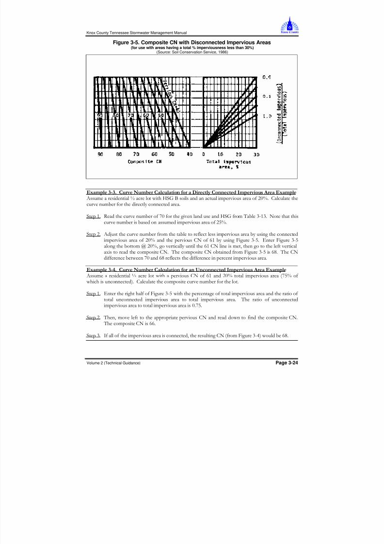
Disconnected Impervious Areas
Runoff from these areas is spread over a pervious area as sheet flow. To determine the CN whenall or part of the impervious area is not directly connected (i.e., “disconnected”) to the drainage
system, either (1) use Figure 3-5 if total impervious area is less than 30% or (2) use Figure 3-4 ifthe total impervious area is equal to or greater than 30%, because the absorptive capacity of theremaining pervious areas will not significantly affect runoff. When impervious area is less than30%, obtain the composite CN by entering the right half of Figure 3-5 with the percentage of totalimpervious area and the ratio of total unconnected impervious area to total impervious area.
Examples 3-3 and 3-4 present the calculation of composite curve numbers for directly connectedand disconnected impervious areas, respectively.
8/11/2019 Vol2 Chap 3 Stormwater Hydrology
http://slidepdf.com/reader/full/vol2-chap-3-stormwater-hydrology 24/76
Knox County Tennessee Stormwater Management Manual
Volume 2 (Technical Guidance) Page 3-24
Figure 3-5. Composite CN with Disconnected Impervious Areas(for use with areas having a total % imperviousness less than 30%)
(Source: Soil Conservation Service, 1986)
& ' ( , - & $ % D # + B C '(!
!
.! , 8' + B 7 . ! E (!
! % F '( ;E /. !
G '( /. ;E ;E! 7 ;E /0! 7
# 8' /0 !
! & ' ( - & $ % D # ;E /. '( # 2! ; !
.! # ! 7 '!8 !
! 7 ;E # 7 ;E //!
! " ;E 1 32 #

8/11/2019 Vol2 Chap 3 Stormwater Hydrology
http://slidepdf.com/reader/full/vol2-chap-3-stormwater-hydrology 25/76
Knox County Tennessee Stormwater Management Manual
Volume 2 (Technical Guidance) Page 3-25
3.1.5.4 Simplified SCS Peak Runoff Rate CalculationThese calculation presented in this section is applicable to drainage areas less than 2,000 acresthat have homogeneous land uses that can be described by a single CN value (SCS, 1986). TheSCS peak discharge equation is presented as Equation 3-16.
Equation 3-16 pu p AQF qQ = where:
Qp = peak discharge (cfs)qu = unit peak discharge (cfs/mi 2 /in)A = drainage area (mi 2)Q = runoff (in)Fp = pond and swamp adjustment factor
The computation sequence for the peak discharge method is presented in steps 1 through 6 below.
1. The 24-hour rainfall depth is determined from rainfall Table 3-5 for the selected location andreturn frequency.
2. The runoff curve number, CN, is estimated from Table 3-13 and direct runoff, Q, is calculatedusing Equation 3-15.
3. The CN value is used to determine the initial abstraction, I a , from Table 3-14, and the ratio I a /Pis then computed (P = accumulated 24-hour rainfall).
Table 3-14. Initial Abstraction (I a) for Runoff Curve NumbersCurve Number I a (in) Curve Number I a (in)
40 3.000 70 0.85741 2.878 71 0.81742 2.762 72 0.77843 2.651 73 0.74044 2.545 74 0.703
45 2.444 75 0.66746 2.348 76 0.63247 2.255 77 0.59748 2.167 78 0.56449 2.082 79 0.53250 2.000 80 0.50051 1.922 81 0.46952 1.846 82 0.43953 1.774 83 0.41054 1.704 84 0.38155 1.636 85 0.35356 1.571 86 0.32657 1.509 87 0.29958 1.448 88 0.27359 1.390 89 0.24760 1.333 90 0.22261 1.279 91 0.19862 1.226 92 0.17463 1.175 93 0.15164 1.125 94 0.12865 1.077 95 0.10566 1.030 96 0.08367 0.985 97 0.06268 0.941 98 0.04169 0.899 -

8/11/2019 Vol2 Chap 3 Stormwater Hydrology
http://slidepdf.com/reader/full/vol2-chap-3-stormwater-hydrology 26/76
Knox County Tennessee Stormwater Management Manual
Volume 2 (Technical Guidance) Page 3-26
4. The watershed time of concentration is computed using the procedures in Section 3.1.3.5 andis used with the ratio I a /P to obtain the unit peak discharge, q u, from Figure 3-6 for the Type IIrainfall distribution. If the ratio I a /P lies outside the range shown in the figure, either use thelimiting values or use another peak discharge method. Note: Figure 3-6 is based on a peakingfactor of 484. If a peaking factor of 300 is needed, this figure is not applicable and thesimplified SCS method should not be used. See Section 3.1.5.5 for additional informationabout peaking factor.
Figure 3-6. SCS Type II Unit Peak Discharge Graph(Source: Soil Conservation Service, 1986)
8/11/2019 Vol2 Chap 3 Stormwater Hydrology
http://slidepdf.com/reader/full/vol2-chap-3-stormwater-hydrology 27/76
Knox County Tennessee Stormwater Management Manual
Volume 2 (Technical Guidance) Page 3-27
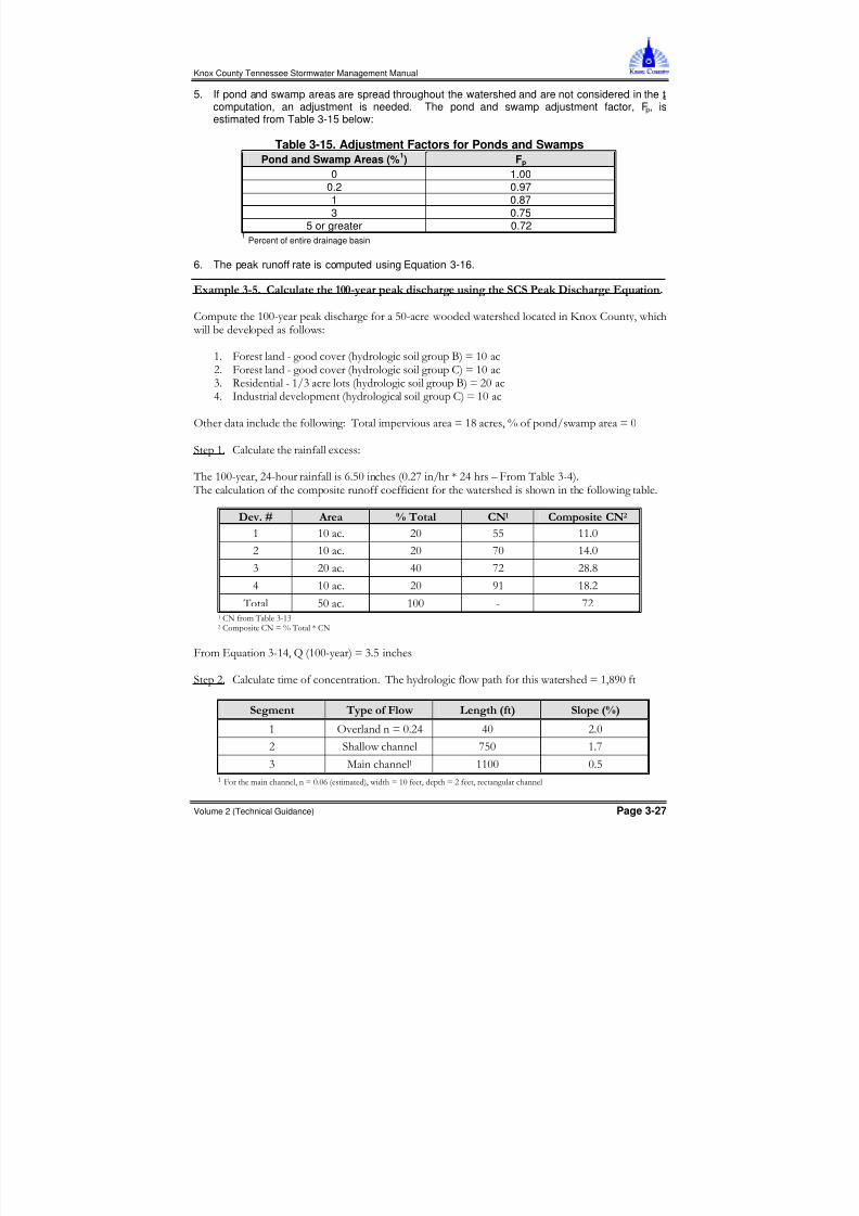
5. If pond and swamp areas are spread throughout the watershed and are not considered in the t c computation, an adjustment is needed. The pond and swamp adjustment factor, F p, isestimated from Table 3-15 below:
Table 3-15. Adjustment Factors for Ponds and Swamps
Pond and Swamp Areas (%1
) F p 0 1.000.2 0.971 0.873 0.75
5 or greater 0.721 Percent of entire drainage basin
6. The peak runoff rate is computed using Equation 3-16.
. // , 0 0 1
; .'' - ' # # H ; # # $
.! 1 C2 & .' ! 1 ;2 & .' ! , .) 1 C2 & '
3! " 1 ;2 & .'
I # $ 7 & .0 ( ) #
.! ; $
7 .'' 3 /! ' 1'! 8 ) J 3 6 7 32!
7 # #
& 2 $ ) # ' ' . .' ! ' ..!'
.' ! ' 8' .3!' ' ! 3' 8 0!0
3 .' ! ' 4. .0! 7 ' ! .'' 8
. ;E 7 . ; ;E & ( 7 J ;E
.3 A 1.'' 2 & ! ! ; ! 7 # # &
0 #, 3 4 " * + 0 *)+
. I & '! 3 3' !' # 8 ' .!8 @ . ..'' '!
. & '!'/ 1 2 # & .' &

8/11/2019 Vol2 Chap 3 Stormwater Hydrology
http://slidepdf.com/reader/full/vol2-chap-3-stormwater-hydrology 28/76
Knox County Tennessee Stormwater Management Manual
Volume 2 (Technical Guidance) Page 3-28
. 7 3 # 5 & ! ' 1'!.3 3 6 7 32 7 & '!''891'! 3213'2: '!0 )1 ! '2 '! 1'!' 2 '!3
& '!.. & /!80
7 8
< & !. ) 1 82 7 & 8 ')91/'21 !.2: & !4
K .' < & 91.!3421.!3 2'!/8 1'!'' 2 '! :)'!'/
& ! ) 7 & ..'')/'1 ! 2 & 0!
7 & /!8 = !4 = 0! & . & '!
& '!.. & /!80
! ; ")5 ;E & 8 2 " & '!880 17 .32
" )5 & 1'!880)/!/'2 & '!. 1E $ K " )5 & '!.' /! !2
3! K 1.'' 2 /& / ' )
! ; - # & . ./
A .'' & / '1 ')/3'21 ! 21.2 & .80
3.1.5.5 Hydrograph GenerationIn addition to estimating the peak discharge, the SCS method can be used to estimate the entirehydrograph from a drainage area. The SCS has developed a Tabular Hydrograph procedure thatcan be used to generate the hydrograph for drainage areas less than 2,000 acres. The TabularHydrograph procedure uses unit discharge hydrographs that have been generated for a series oftime of concentrations. In addition, SCS has developed hydrograph procedures to be used togenerate composite flood hydrographs. For hydrograph development in homogeneous developeddrainage areas, for hydrograph development for drainage areas that are not homogeneous andwhere multiple sub-area hydrographs need to be generated, routed and combined at a pointdownstream (SCS, 1986),
The unit hydrograph equations used in the SCS method for generating hydrographs include aconstant to account for the general land slope in the drainage area. This constant, called apeaking factor, can be adjusted when using the method. A default value of 484 for the peakingfactor represents rolling hills – a medium level of relief. SCS indicates that for mountainous terrain
the peaking factor can go as high as 600, and as low as 300 for flat (coastal) areas. In KnoxCounty, the default value of 484 must be used for the peaking factor.
The development of a runoff hydrograph from a watershed is a laborious process not normallydone by hand. For that reason this discussion is limited to an overview of the process and is givenhere to assist the designer in reviewing and understanding the input and output from a typicalcomputer program. There are choices of computational interval, storm length (if the 24-hour stormis not going to be used) and other “administrative” parameters that are specific to each computerprogram.

8/11/2019 Vol2 Chap 3 Stormwater Hydrology
http://slidepdf.com/reader/full/vol2-chap-3-stormwater-hydrology 29/76
Knox County Tennessee Stormwater Management Manual
Volume 2 (Technical Guidance) Page 3-29
The development of a runoff hydrograph for a watershed or one of many sub-basins within a morecomplex model involves the following steps:
1. Development or selection of a design storm hyetograph (a graph of the time distribution ofrainfall over a watershed). Often, the SCS 24-hour storm described in Section 3.1.5.3 is used.
2. Development of curve numbers and lag times for the watershed using the methods describedin Sections 3.1.5.4, 3.1.5.5, and 3.1.5.6.
3. Development of a unit hydrograph from the standard (peaking factor of 484) dimensionless unithydrographs. See discussion below.
4. Step-wise computation of the initial and infiltration rainfall losses and, thus, the excess rainfallhyetograph using a derivative form of the SCS rainfall-runoff equation (Equation 3-12).
5. Application of each increment of excess rainfall to the unit hydrograph to develop a series ofrunoff hydrographs, one for each increment of rainfall (this is called “convolution”).
6. Summation of the flows from each of the small incremental hydrographs (keeping proper trackof time steps) to form a runoff hydrograph for that watershed or sub-basin.
Figure 3-7 and Table 3-16 can be used along with Equations 3-17 and 3-18 to assist the designer inusing the SCS unit hydrograph in Knox County. The unit hydrograph with a peaking factor of 300 isshown in the figure for comparison purposes, but should not be used for areas in Knox County.
Figure 3-7. Dimensionless Unit Hydrographs for Peaking Factors of 484 and 300

8/11/2019 Vol2 Chap 3 Stormwater Hydrology
http://slidepdf.com/reader/full/vol2-chap-3-stormwater-hydrology 30/76
Knox County Tennessee Stormwater Management Manual
Volume 2 (Technical Guidance) Page 3-30
Table 3-16. Dimensionless Unit Hydrograph 484484t/T p
q/q u Q/Qp0.0 0.000 0.0000.1 0.005 0.0000.2 0.046 0.0040.3 0.148 0.0150.4 0.301 0.0380.5 0.481 0.0750.6 0.657 0.1250.7 0.807 0.1860.8 0.916 0.2550.9 0.980 0.3301.0 1.000 0.4061.1 0.982 0.4811.2 0.935 0.5521.3 0.867 0.6181.4 0.786 0.6771.5 0.699 0.7301.6 0.611 0.7771.7 0.526 0.8171.8 0.447 0.8511.9 0.376 0.8792.0 0.312 0.9032.1 0.257 0.9232.2 0.210 0.9392.3 0.170 0.9512.4 0.137 0.962
2.5 0.109 0.9702.6 0.087 0.9772.7 0.069 0.9822.8 0.054 0.9862.9 0.042 0.9893.0 0.033 0.9923.1 0.025 0.9943.2 0.020 0.9953.3 0.015 0.9963.4 0.012 0.9973.5 0.009 0.9983.6 0.007 0.998
3.7 0.005 0.9993.8 0.004 0.9993.9 0.003 0.9994.0 0.002 1.000
Equation 3-17 is used to multiply each time ratio value by the time-to-peak (T p) and each value ofq/q u by q u.
Equation 3-17 p
u T APF
q )(
=
8/11/2019 Vol2 Chap 3 Stormwater Hydrology
http://slidepdf.com/reader/full/vol2-chap-3-stormwater-hydrology 31/76
Knox County Tennessee Stormwater Management Manual
Volume 2 (Technical Guidance) Page 3-31
where:qu = unit hydrograph peak rate of discharge (cfs)PF = peaking factor (either 484 or 300)A = area (mi 2)Tp = time to peak = d/2 + 0.6 T c (hours)d = rainfall time increment (hours)
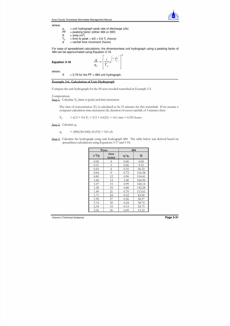
For ease of spreadsheet calculations, the dimensionless unit hydrograph using a peaking factor of484 can be approximated using Equation 3-18.
Equation 3-18
X
T t
pu
peT t
=
−1
where:X = 3.79 for the PF = 484 unit hydrograph.
5 6,
; ' # # !
; .! ; 71 -2
7 17 2 . # ! " # 1 2
7 & ) = '!/ 7 & ) = '!/1 .2 & .3!. & '!
! ;
& 130321 ')/3'2)1'! 2 & ./.
! ; 303! 7 # # .8 .0!
# !7!
8# * + 181 9
'!'' ' '!'' '!'''! . '!'/ 4!.'!3 / '! /!'!/3 4 '!8 ../! 0
'!0 . '!4/ . 3!3..!'' .3 .!'' ./'!4'.!'8 . '!44 ./'!.3.! 0 .0 '!00 .3 ! 0.!34 . '!8' .. !/..!8. 3 '! 0 !4'.!4 8 '! / 0! 8
!.3 ' '! 3 0!83! '!. 3!8! / / '!'4 . !

8/11/2019 Vol2 Chap 3 Stormwater Hydrology
http://slidepdf.com/reader/full/vol2-chap-3-stormwater-hydrology 32/76
Knox County Tennessee Stormwater Management Manual
Volume 2 (Technical Guidance) Page 3-32
# !7!
8# * + 181 9
!80 4 '!'/ 4! 3!44 3 '!' !3! ' 3 '!' !.!3 30 '!'. .!84!/ . '!'. .!''!03 3 '!'' '!
3!'/ 8 '!'' '! '3! 8 /' '!'' '!./3!30 / '!'' '!'43!8' // '!'' '!'3!4. /4 '!'' '!'
3.1.6 Clark Unit Hydrograph
In Knox County, use of the Clark Unit Hydrograph method is acceptable only for hydrologiccalculations that are prepared for flood studies and flood elevation calculations. See Volume 2,Chapter 9 for more information on flood study preparation.
The Clark method defines a unit hydrograph for a given basin using the concept of theinstantaneous unit hydrograph (IUH). An IUH is a theoretical hydrograph that would result when asingle unit of rainfall excess was spread out evenly over an entire basin and allowed to run off. TheIUH can be converted to a unit hydrograph of a desired duration by conventional techniques fordeveloping unit hydrographs (Hoggan, 1997).
The Clark method is based on the effects of translation and attenuation as the primary forcesinvolved in the flow of water through a watershed. Translation is defined as the ‘downhill’ flow ofwater as a result of the force of gravity. Attenuation is defined as the resistance of flow that iscaused by either friction in the channel or water storage. According to Clark, translation in awatershed can be described with a time-area curve. This curve displays the portion of watershedarea that is contributing runoff as a function of time. The curve should start at the point in whicheffective precipitation begins. Effective precipitation is any precipitation that does not infiltrate intothe soil or is retained in a ponding area. Equation 3-19 presents these concepts.
Equation 3-19 ROS =
where:S = StorageR = Attenuation (Watershed Storage) ConstantO = Outflow
A synthetic hydrograph could be produced by proportionally routing an inch of direct runoff to thechannel in accordance with the time-area curve. The runoff entering the channel would then berouted through a linear reservoir. More recent studies have indicated that it is not necessary toproduce detailed time-area curves in order to produce accurate synthetic hydrographs. Thedimensionless time-area curve included in HEC-1 and HEC-HMS hydrologic models (developed bythe United States Army Corps of Engineers) have produced accurate synthetic hydrographs. Inorder to apply the Clark method in a HEC-1 or HEC-HMS model, the time of concentration (tc) anda watershed storage constant (R) are required as inputs. In stormwater master plans prepared forKnox County in the late 1990’s and early 2000’s, research indicated that Equation 3-20, whichequates to setting R = T c, produced accurate estimates of peak discharges for small drainage

8/11/2019 Vol2 Chap 3 Stormwater Hydrology
http://slidepdf.com/reader/full/vol2-chap-3-stormwater-hydrology 33/76
Knox County Tennessee Stormwater Management Manual
Volume 2 (Technical Guidance) Page 3-33
areas. However, the engineer performing the flood study should determine the most appropriateequation to determine the value of R.
Equation 3-20 5.0=+ RT
R
c
where:R = Attenuation (Watershed Storage) ConstantTc = Time of concentration
3.1.7 Water Quality Calculations
3.1.7.1 Water Quality Volume CalculationIn Knox County, the Water Quality Volume (WQv) is the treatment volume required to remove 80%of the average annual, post-development total suspended solids (TSS) load. This is achieved byintercepting and treating a portion of the runoff from all storms and all the runoff from 85% of thestorms that occur on average during the course of a year. The water quality treatment volume iscalculated using Equation 3-21.
Equation 3-21 121.1 A RWQv v=
where:WQv = water quality volume (acre-feet)1.1 = the 85 th percentile annual rainfall depth in Knox County (inches)Rv = volumetric runoff coefficient (see Equation 3-22)A = total drainage area (acres)
The volumetric runoff coefficient (Rv) is directly proportional to the percent impervious cover of thedevelopment or drainage area. Rv is calculated using Equation 3-22.
Equation 3-22 ( ) I Rv 0092.0015.0 +=
where:I = percent of impervious cover (%)
3.1.7.2 Water Quality Peak Discharge CalculationThe peak rate of discharge for the water quality design storm (Q wq, also called the water qualitypeak discharge) is needed to size off-line diversion structures, such as for sand filters andinfiltration trenches. This method is utilized for the sizing of water quality treatment controls asopposed to more traditional peak discharge calculation methods which are not appropriate for thisapplication. For example, the use of the Rational Method for sizing water quality controls wouldrequire the choosing of an arbitrary storm event. Further, conventional SCS methods have beenfound to underestimate the volume and rate of runoff for rainfall events of less than two inches.This discrepancy in estimating runoff and discharge rates can lead to situations where a significantamount of runoff bypasses the structural control due to an inadequately sized diversion structureand leads to the design of undersized bypass channels.
Equation 3-23 is utilized to calculate Q wq.
Equation 3-23 wvuwq AQqQ =
where:Qwq = the water quality flow rate (cfs)qu = the unit peak discharge (cfs/mi²/inch)A = drainage area (mi 2)Qwv = runoff peak volume (water quality volume), in inches (1.1R v)

8/11/2019 Vol2 Chap 3 Stormwater Hydrology
http://slidepdf.com/reader/full/vol2-chap-3-stormwater-hydrology 34/76
Knox County Tennessee Stormwater Management Manual
Volume 2 (Technical Guidance) Page 3-34
The following procedure can be used to calculate Q wq. This procedure relies on WQv and thesimplified peak discharge calculation: WQv (water quality volume in acre-feet) = Q wv (water qualityrunoff peak volume in inches) =1.1Rv. An example calculation is provided in Example 3-7.
1. Using Q wv=1.1(Rv), a corresponding CN is computed utilizing a form of Equation 3-15:
CN = 1000/[10 + 5P + 10Q wv - 10(Q wv2 +1.25 Q wvP) 0.5]
where:P = 1.1 inchesQwv = water quality runoff peak volume (inches)
2. Once a CN is computed, the time t c is computed.
3. Using the computed CN, t c and drainage area (A), in acres; the water quality peak discharge(Qwq) is computed using a slight modification to the Simplified SCS Peak Runoff RateEstimation technique discussed previously. The following steps will apply to the calculation.
a. read initial abstraction (I a), compute I a /P;
b. read the unit peak discharge (q u) for appropriate t c; andc. using Q wv, compute the water quality flow rate (Q wq) using Equation 3-23.
: % 9 , ; % 9 , 3 4K ?A A # !
.$ ; , $
, & '!'. =1'!''4 21"2 & '!'. =1'!''4 '1.0) '21.''2 & '!
$ ; # ?A $
?A & .!., %). & .!.1'! 21 '2). & .!/
! ; - A # $
A # & .!., & .!.1'! 2 & '! 4
3$ ; $
;E & .''')9.' = 1.!.2 = .'1'! 42 6 .'91'! 42 =.! 1'! 421.!.2:'! & 4' & .''')1;E 6 .'2 & .''')14' .'2 & .!..
'! & " & '! " )5 & '! ).!. & '! '
$ & '! / ")5 & '! '
& 0' ) )
/$ ; # - # !
A # & 0'1 ')/3'21'! 42 & .8!/8

8/11/2019 Vol2 Chap 3 Stormwater Hydrology
http://slidepdf.com/reader/full/vol2-chap-3-stormwater-hydrology 35/76
Knox County Tennessee Stormwater Management Manual
Volume 2 (Technical Guidance) Page 3-35
3.1.8 Water Balance Calculations
Water balance calculations can help to determine if a drainage area is large enough or has theright characteristics to support a permanent pool of water during average or extreme conditions.When in doubt, a water balance calculation may be advisable for retention pond and wetlanddesign.
The details of a rigorous water balance are beyond the scope of this manual. However, asimplified procedure is described herein that will provide an estimate of pool viability and point tothe need for more rigorous analysis. Water balance can also be used to help establish plantingzones in a wetland design.
3.1.8.1 Basic EquationsWater balance is defined as the change in volume of the permanent pool resulting from the totalinflow minus the total outflow (actual or potential). Equation 3-24 presents this calculation.
Equation 3-24 −=∆ O I V
where: ∆ = delta or “change in”V = pond volume (ac-ft)Σ = “the sum of”I = Inflows (ac-ft)O = Outflows (ac-ft)
The inflows consist of rainfall, runoff and baseflow into the pond. The outflows consist ofinfiltration, evaporation, evapotranspiration, and surface overflow out of the pond or wetland.Equation 3-24 can be expanded to reflect these factors, as shown in Equation 3-25. Key variablesin Equation 3-25 are discussed in detail below the equation.
Equation 3-25 Of EtA EA IA Bf RPAV o −−−−++=∆
where:P = precipitation (ft)A = area of pond (ac)Ro = runoff (ac-ft)Bf = baseflow (ac-ft)I = infiltration (ft)E = evaporation (ft)Et = evapotranspiration (ft)Of = overflow (ac-ft)
Rainfall (P) – Monthly rainfall values can be obtained from the National Weather Serviceclimatology at http://www.srh.noaa.gov/mrx/climat.htm . Monthly values are commonly used for
calculations of values over a season. Rainfall is then the direct amount that falls on the pondsurface for the period in question. When multiplied by the pond surface area (in acres) it becomesacre-feet of volume. Table 3-17 presents average monthly rainfall values for Knoxville based on a30-year period of record.
Table 3-17. Average Rainfall Values in Inches for Knoxville, TennesseeJan Feb Mar Apr May Jun Jul Aug Sep Oct Nov Dec
P (feet) 4.57 4.01 5.17 3.99 4.68 4.04 4.71 2.89 3.04 2.65 3.98 4.49
Annual Precipitation 48.2 Source: www.ncdc.noaa.gov/oa/climate/online/ccd/nrmpcp.txt

8/11/2019 Vol2 Chap 3 Stormwater Hydrology
http://slidepdf.com/reader/full/vol2-chap-3-stormwater-hydrology 36/76
Knox County Tennessee Stormwater Management Manual
Volume 2 (Technical Guidance) Page 3-36
Runoff (R o) – Runoff is equivalent to the rainfall for the period times the “efficiency” of thewatershed, which is equal to the ratio of runoff to rainfall (Q/P). In lieu of gage information, Q/P canbe estimated one of several ways. The best method would be to perform long-term simulationmodeling using rainfall records and a watershed model.
Equation 3-21 gives a ratio of runoff to rainfall volume for a particular storm. If it can be assumedthat the average storm that produces runoff has a similar ratio, then the Rv value can serve as theratio of rainfall to runoff. Not all storms produce runoff in an urban setting. Typical initial losses(often called “initial abstractions”) are normally taken between 0.1 and 0.2 inches. When comparedto the rainfall records in Knox County, this is equivalent to about a 10% runoff volume loss. Thus,in a water balance calculation, a factor of 0.9 should be applied to the calculated Rv value toaccount for storms that produce no runoff. Equation 3-26 reflects this approach. Total runoffvolume is then simply the product of runoff depth (Q) times the drainage area to the pond.
Equation 3-26 PRvQ 9.0=
where:Q = runoff volume (in)P = precipitation (in)Rv = volumetric runoff coefficient [Equation 3-22]
Baseflow (B f) – Most stormwater ponds and wetlands have little, if any, baseflow, as they are rarelyplaced across perennial streams. If so placed, baseflow must be estimated from observation orthrough theoretical estimates. Methods of estimation and baseflow separation can be found inmost hydrology textbooks.
Infiltration (I) – Infiltration is a very complex subject and cannot be covered in detail here. Theamount of infiltration depends on soils, water table depth, rock layers, surface disturbance, thepresence or absence of a liner in the pond, and other factors. The infiltration rate is governed bythe Darcy equation, shown in Equation 3-27.
Equation 3-27 hh G Ak I =
where:I = infiltration (ac-ft/day)A = cross sectional area through which the water infiltrates (ac)kh = saturated hydraulic conductivity or infiltration rate (ft/day)Gh = hydraulic gradient = pressure head/distance
Gh can be set equal to 1.0 for pond bottoms and 0.5 for pond sides steeper than about 4:1.Infiltration rate can be established through testing, though not always accurately. Table 3-18 canbe used for initial estimation of the saturated hydraulic conductivity.
Table 3-18. Saturated Hydraulic Conductivity(Source: Ferguson and Debo, 1990)
Hydraulic ConductivityMaterialin/hr ft/day
ASTM Crushed Stone No. 3 50,000 100,000ASTM Crushed Stone No. 4 40,000 80,000ASTM Crushed Stone No. 5 25,000 50,000ASTM Crushed Stone No. 6 15,000 30,000Sand 8.27 16.54Loamy sand 2.41 4.82Sandy loam 1.02 2.04Loam 0.52 1.04

8/11/2019 Vol2 Chap 3 Stormwater Hydrology
http://slidepdf.com/reader/full/vol2-chap-3-stormwater-hydrology 37/76
Knox County Tennessee Stormwater Management Manual
Volume 2 (Technical Guidance) Page 3-37
Hydraulic ConductivityMaterialin/hr ft/day
Silt loam 0.27 0.54Sandy clay loam 0.17 0.34Clay loam 0.09 0.18
Silty clay loam 0.06 0.12Sandy clay 0.05 0.10Silty clay 0.04 0.08Clay 0.02 0.04
Evaporation (E) – Evaporation is from an open lake water surface. Evaporation rates aredependent on differences in vapor pressure, which, in turn, depend on temperature, wind,atmospheric pressure, water purity, and shape and depth of the pond. It is estimated or measuredin a number of ways, which can be found in most hydrology textbooks. Pan evaporation methodsare also used, though there are no longer pan evaporation sites active in Knox County. Formerlypan evaporation methods were utilized at the Knoxville Experiment Station.
Table 3-19 presents pan evaporation rate distributions for a typical 12-month period based on panevaporation information from one station in Knox County. Figure 3-8 depicts a map of annual freewater surface (FWS) evaporation averages for Tennessee based on a National Oceanic andAtmospheric Administration (NOAA) assessment done in 1982. FWS evaporation differs from lakeevaporation for larger and deeper lakes, but can be used as an estimate of it for the type ofstructural stormwater ponds and wetlands being designed in Knox County. Total annual valuescan be estimated from this map and distributed in accordance with the percentages presented inTable 3-19 .
Table 3-19. Pan Evaporation Rates - Monthly DistributionJan Feb Mar Apr May Jun Jul Aug Sep Oct Nov Dec
2.9% 3.8% 7.2% 10.6% 13.1% 13.1% 13.2% 12.4% 9.8% 6.7% 4.1% 3.1%
Figure 3-8. Average Annual Free Water Surface Evaporation (in inches)(Source: NOAA, 1982)

8/11/2019 Vol2 Chap 3 Stormwater Hydrology
http://slidepdf.com/reader/full/vol2-chap-3-stormwater-hydrology 38/76
Knox County Tennessee Stormwater Management Manual
Volume 2 (Technical Guidance) Page 3-38
Evapotranspiration (E t). Evapotranspiration consists of the combination of evaporation andtranspiration by plants. The estimation of E t for crops is well documented and has becomestandard practice. However, the estimating methods for wetlands are not documented, nor arethere consistent studies to assist the designer in estimating the wetland plant demand on watervolumes. Literature values for various places in the United States vary around the free watersurface lake evaporation values. Estimating E t only becomes important when wetlands are beingdesigned and emergent vegetation covers a significant portion of the pond surface. In these casesconservative estimates of lake evaporation should be compared to crop-based E t estimates and adecision made. Crop-based E t estimates can be obtained from typical hydrology textbooks or fromthe web sites mentioned above. A value of zero shall be assumed for E t unless the wetland designdictates otherwise.
Overflow (O f) – Overflow is considered as excess runoff, and in water balance design is either notconsidered since the concern is for average precipitation values, or is considered lost for allvolumes above the maximum pond storage. Obviously, for long-term simulations of rainfall-runoff,large storms would play an important part in pond design.
7 % < H / H ; #
! 7 #! 7 # ! ? L #
8 ( # !
.$ , & '!'. = '!''4 18 2 & '!8.! ? '!4 # '!/3! 7 - 0 ! !
" & '! 3 ) 17 .02! - # .'(
@ H ; # ? !
$ 7 # #
; = 3 ( $ , = = $ 0 > ' &
. @ . 0 . ' . ' . . ' . ' .
5 !1 2 3! 8 3!'. !.8 !44 3!/0 3!'3 3!8. !04 !'3 !/ !40 3!34
!! 1(2 !4 !0 8! .'!/ . !. . !. . ! . !3 4!0 /!8 3!. !.
3 , '
1 2 /! ! / 8!./ ! /!34 !/' /! 3!'. 3! . !/0 ! /!
51 2 '!.4 '!.8 '! '!.8 '! ' '!.8 '! ' '!. '!. '!.. '!.8 '!.4
/ 1 2 '!'/ '!'0 '!.3 '! '! / '! / '! / '! '! ' '!. '!'0 '!'/
8 "1 2 !'. 3! !'. 3!0 !'. 3!0 !'. !'. 3!0 !'. 3!0 !'.
0 C !1 2 .!3 .!. ! '!/ .!3 '!// .!3/ .!. '!8. .! '!8/ .!
4 , ! C !1 2 .!3 !'' !'' !'' !'' !'' !'' '!08 '!./ ' '!8/ !''
7 $.!

8/11/2019 Vol2 Chap 3 Stormwater Hydrology
http://slidepdf.com/reader/full/vol2-chap-3-stormwater-hydrology 39/76
Knox County Tennessee Stormwater Management Manual
Volume 2 (Technical Guidance) Page 3-39
! @ # # 7 .8!! 7 .4!
3! ? '!/3 1/2!
! 5
. !/! 30 8! " 4'(
'! 1C - 3$.2 .'( !0! C * 13 = 2 1/ = 82!4! , C 4 -
# !
" ! 7 #
!
3.1.9 Calculating Downstream Impacts (the Ten Percent Rule)
In the Knox County Stormwater Management Manual, the “ten-percent” rule has been adopted asthe approach for ensuring that stormwater quantity detention ponds maintain pre-developmentpeak flows through the downstream conveyance system.
The ten-percent rule recognizes the fact that a structural control providing detention has a “zone ofinfluence” downstream where its effectiveness can be observed. Beyond this zone of influence thestructural control becomes relatively small and insignificant compared to the runoff from the totaldrainage area at that point. Based on studies and master planning results for a large number ofsites, that zone of influence is considered to be the point where the drainage area controlled by thedetention or storage facility comprises 10% of the total drainage area. For example, if thestructural control drains 10 acres, the zone of influence ends at the point where the total drainagearea is 100 acres or greater.
Typical steps in the application of the ten-percent rule are:
1. Using a topographic map determine the lower limit of the “zone of influence” (i.e., the 10%point), and determine all 10% rule comparison points (at the outlet of the site and at alldownstream tributary junctions).
2. Using a hydrologic model determine the pre-development peak discharges (pre-Qp 2, pre-Qp 10 ,pre-Qp 25 , and pre-Qp 100 ) and timing of those peaks at each tributary junction beginning at thepond outlet and ending at the next tributary junction beyond the 10% point.
3. Change the site land use to post-development conditions and determine the post-developmentpeak discharges (post-Qp 2, post-Qp 10 , post-Qp 25 , and post-Qp 100 ). Design the structuralcontrol facility such that the post-development peak discharges from the site for all storm
events do not increase the pre-development peak discharges at the outlet of the site and ateach downstream tributary junction and each public or major private downstream stormwaterconveyance structure located within the zone of influence.
4. If post-development conditions do increase the peak flow within the zone of influence, thestructural control facility must be redesigned or one of the following options must be chosen:
• Control of the Qp 2, Qp 10 , Qp 25 , and/or Qp 100 may be waived by the Director of Engineeringand Public Works (the Director) if adequate overbank flood protection and/or extreme floodprotection is suitably provided by a downstream or shared off-site stormwater facility, or ifengineering studies determine that installing the required stormwater facilities would not bein the best interest of Knox County. However, a waiver of such controls does not eliminate

8/11/2019 Vol2 Chap 3 Stormwater Hydrology
http://slidepdf.com/reader/full/vol2-chap-3-stormwater-hydrology 40/76

8/11/2019 Vol2 Chap 3 Stormwater Hydrology
http://slidepdf.com/reader/full/vol2-chap-3-stormwater-hydrology 41/76
Knox County Tennessee Stormwater Management Manual
Volume 2 (Technical Guidance) Page 3-41
C # # .4' ! / ! 7 F # .'( F
# ! 7 .4' # - 7, ' # ! 7
# - # .
3.2 Storage Design 3.2.1 General Storage Concepts
This section provides general guidance on stormwater runoff storage for meeting control of theWQv, CPv, Qp 2, Qp 10 , Qp 25 and the Qp 100 . Storage of stormwater runoff within a stormwatermanagement system is critical to providing the extended detention of flows for water qualitytreatment and downstream channel protection, as well as for peak flow attenuation of the largeroverbank and extreme flood protection flows. Runoff storage can be provided within an on-sitesystem through the use of structural stormwater BMPs and/or non-structural features andlandscaped areas. Figure 3-9 illustrates various storage facilities that can be considered for adevelopment site.
Figure 3-9. Examples of Typical Stormwater Storage Facilities
Dry Basin
Stormwater Pond or Wetland
Flood Level
Flood Level
Permanent Pool
Rooftop Storage
LandscapedArea
Parking LotStorage
Underground Vault Underground StoragePipe
There are three main types of stormwater runoff storage: detention, extended detention, andretention . Stormwater detention is used to reduce the peak discharge and detain runoff for aspecified short period of time. Detention basins are designed to completely drain after the designstorm has passed. Detention is used to meet overbank flood protection criteria, and extreme floodcriteria where required. Extended detention (ED) is used to drain a runoff volume over a specifiedperiod of time, typically 24 hours, and is used to meet channel protection criteria. Some structuralBMP designs (wet ED pond, micropool ED pond, dry extended pond and shallow ED marsh) alsoinclude extended detention storage of a portion of the water quality volume. Retention facilities,
8/11/2019 Vol2 Chap 3 Stormwater Hydrology
http://slidepdf.com/reader/full/vol2-chap-3-stormwater-hydrology 42/76
Knox County Tennessee Stormwater Management Manual
Volume 2 (Technical Guidance) Page 3-42
such as stormwater ponds and wetlands, are designed to contain a permanent pool of water that isused for water quality treatment. Some facilities include one or more types of storage. An exampleof a combined storage facility is one that is sized to provide extended detention of the WQv as wellas detention of the Qp 100 .
Storage facilities are often classified on the basis of their location and size. On-site storage isconstructed on individual development sites and most often only provides control of the runoff thatdischarges that individual site. Regional storage facilities are designed to manage stormwaterrunoff from multiple projects and/or properties, or are constructed at the lower end of a sub-basinwithin which multiple properties are located. Knox County Engineering will determine if the use of aregional storage facility is applicable on a case-by-case basis.
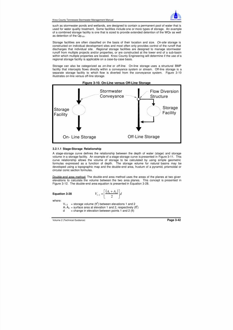
Storage can also be categorized as on-line or off-line . On-line storage uses a structural BMPfacility that intercepts flows directly within a conveyance system or stream. Off-line storage is aseparate storage facility to which flow is diverted from the conveyance system. Figure 3-10illustrates on-line versus off-line storage.
Figure 3-10. On-Line versus Off-Line Storage
StormwaterConveyance
Flow DiversionStructure
Off-Line StorageOn- Line Storage
StorageFacility
StorageFacility
3.2.1.1 Stage-Storage Relationship
A stage-storage curve defines the relationship between the depth of water (stage) and storagevolume in a storage facility. An example of a stage-storage curve is presented in Figure 3-11. Thiscurve relationship allows the volume of storage to be calculated by using simple geometricformulas expressed as a function of depth. The storage volume for natural basins may bedeveloped using a topographic map and the double-end area, frustum of a pyramid, prismoidal orcircular conic section formulas.
Double-end area method: The double-end area method uses the areas of the planes at two givenelevations to calculate the volume between the two area planes. This concept is presented inFigure 3-12. The double-end area equation is presented in Equation 3-28.
Equation 3-28( )
d A A
V +
=− 221
21
where:V1-2 = storage volume (ft 3) between elevations 1 and 2A1 A2 = surface area at elevation 1 and 2, respectively (ft 2)
d = change in elevation between points 1 and 2 (ft)

8/11/2019 Vol2 Chap 3 Stormwater Hydrology
http://slidepdf.com/reader/full/vol2-chap-3-stormwater-hydrology 43/76
Knox County Tennessee Stormwater Management Manual
Volume 2 (Technical Guidance) Page 3-43
Figure 3-11. Stage-Storage Curve
Figure 3-12. Double-End Area Method
A3
A2
A1
AREA AT 103 ft
100 ft
101 ft
102 ft
103 ft
AREA AT 102 ft
AREA AT 101 ft
ZERO AREA AT 100 ft
d
Frustrum of a pyramid method: Another calculation involves treating the storage as a pyramidfrustum, or a part of a pyramid. The frustum is formed by truncating the pyramid using two planesparallel to the pyramid base. The frustum of a pyramid can be calculated using Equation 3-29.
Stage (ft)
S t o r a g e
( a c - f t )
100 101 102 103 104 105 106 107
12.0
10.0
8.0
6.0
4.0
2.0
0.0

8/11/2019 Vol2 Chap 3 Stormwater Hydrology
http://slidepdf.com/reader/full/vol2-chap-3-stormwater-hydrology 44/76
Knox County Tennessee Stormwater Management Manual
Volume 2 (Technical Guidance) Page 3-44
Equation 3-29 ( )[ ]25.0
2113 A A A A
d V +×+=
where:V = volume of frustum of a pyramid (ft 3)
d = change in elevation between points 1 and 2 (ft)
A1 = surface area at elevation 1 (ft2
)A2 = surface area at elevation 2 (ft 2)
Frustrum of a prismoid method: A trapezoidal basin can be represented as a prismoid since thevolume is formed by the trapezoidal faces. Equation 3-30 presents the prismoidal equation fortrapezoidal basins.
Equation 3-30 ( ) 322
3
4 D Z ZDW L LWDV +++=
where:V = volume of trapezoidal basin (ft 3)
L = length of basin at base (ft)W = width of basin at base (ft)
D = depth of basin (ft)Z = side slope factor, ratio of horizontal to vertical
Frustrum of a cone or conic section method: Equations 3-31 and 3-32 present the calculationapproach for the basin storage volume represented is as a circular cone.
Equation 3-31 ( )212
22
1047.1 R R R R DV ++=
Equation 3-32 221
21 33047.1 D Z ZDR R DV ++=
where:V = volume of circular cone basin (ft 3)R
1, R
2= bottom and surface radii of the conic section (ft)
D = depth of basin (ft)Z = side slope factor, ratio of horizontal to vertical
3.2.1.2 Stage-Discharge RelationshipA stage-discharge curve defines the relationship between the depth of water and the discharge oroutflow from a storage facility. Figure 3-13 presents an example stage-discharge curve. A typicalstorage facility has multiple outlets or spillways: a principal outlet that handles the range of designstorms and design criteria and a secondary (or emergency) outlet. The principal outlet is usuallydesigned with a capacity sufficient to convey the design discharges and volumes without allowingflow to enter the emergency spillway. Pipes, culverts, weirs, perforated risers and otherappropriate outlets can be used in the principal spillway or outlet.
The emergency spillway is sized to provide a bypass for floodwater during a flood that exceeds thedesign capacity of the principal outlet. This spillway should be designed taking into account thepotential threat to downstream areas if the storage facility were to fail. The stage-discharge curveshould take into account the discharge characteristics of both the principal spillway and theemergency spillway. For more details, see Section 3.3 of this chapter.
3.2.2 Symbols and Definitions
To provide consistency within this section, the symbols listed in Table 3-20 will be used. Thesesymbols were selected because of their wide use in technical publications. In some cases, thesame symbol is used in existing publications for more than one definition. Where this occurs in thissection, the symbol will be defined where it occurs in the text or equations.

8/11/2019 Vol2 Chap 3 Stormwater Hydrology
http://slidepdf.com/reader/full/vol2-chap-3-stormwater-hydrology 45/76
Knox County Tennessee Stormwater Management Manual
Volume 2 (Technical Guidance) Page 3-45
Figure 3-13. Example Stage-Discharge Curve
Stage (ft)
D i s c
h a r g e
( c f s )
100 101 102 103 104 105 106 107
300
250
200
150
100
50
0
Table 3-20. Symbols and Definitions for Storage DesignSymbol Definition Units
a,b Rainfall factors for Modified Rational Method -A Cross sectional or surface area ft 2 A Drainage area acres (or mi 2)
Cw Weir coefficient -C Rational Method Runoff Coefficient -
CN Curve number -CPv Channel protection volume acre-ft
d Change in elevation ftD Depth of basin or diameter of pipe ftg Acceleration due to gravity ft/s 2 H Head on structure ftHC Height of weir crest above channel bottom ft
i Rainfall intensity in/hrL Length ftP x Storm depth for x duration storm in
q i,q o Peak inflow or outflow rate cfs, inR Surface Radii ft
Rv Runoff coefficient -t Routing time period sec
tb Time base of hydrograph sec, hrtc Time of concentration minTd Critical storm duration minTi Duration of basin inflow hr, min, sectP Time to peak of hydrograph hrTt Travel time min
V, V s Storage volume ft 3, acre-ftVr Runoff volume ft 3, acre-ftW Width of basin ft
WQv Water quality volume acre-ftZ Side slope factor -

8/11/2019 Vol2 Chap 3 Stormwater Hydrology
http://slidepdf.com/reader/full/vol2-chap-3-stormwater-hydrology 46/76
Knox County Tennessee Stormwater Management Manual
Volume 2 (Technical Guidance) Page 3-46
3.2.3 General Storage Design Procedures
This section discusses the general design procedures for designing storage to provide standarddetention of stormwater runoff for the Qp 2, Qp 10 , Qp 25 and Qp 100 . The design procedures for allstorage facilities are the same whether or not they include a permanent pool of water. In the lattercase, the permanent pool elevation is taken as the “bottom” of storage and is treated as if it were a
solid basin bottom for routing purposes.
The location of a storage facility can have a sizeable impact on the effectiveness of such facilitiesto control downstream impacts. In addition, multiple storage facilities located in the same drainagebasin will affect the timing of the runoff through the downstream conveyance system, which coulddecrease or increase flood peaks in different downstream locations. Therefore, a downstreampeak flow analysis (i.e., the 10% rule) should be performed as part of the storage facility designprocess. In multi-purpose multi-stage facilities such as stormwater ponds, the storage design mustbe integrated with the overall design for water quality treatment objectives. See Volume 2, Chapter4 for further guidance and criteria for the design of structural best management practices (BMPs)for water quality control.
3.2.3.1 Design Procedure
The following data are needed for storage design and routing calculations:
• inflow hydrograph for all selected design storms;
• stage-storage curve for proposed storage facility; and
• stage-discharge curve(s) for all outlet control structures.
A general procedure for using the above data in the design of storage facilities is presented below.
1. Compute inflow hydrographs for the 2, 10, 25 and 100-year, 24-hour design storms using thehydrologic methods outlined in Section 3.1. Both existing conditions and post-developmenthydrographs are required.
2. Perform preliminary calculations to evaluate detention storage requirements for thehydrographs from Step 1.
3. Determine the physical basin dimensions necessary to hold the volumes determined in Step 2,including freeboard, which is defined as 1.0 foot above the Qp 100 water surface elevation to thelowest point in the detention embankment, excluding the emergency spillway. The maximumstorage requirement calculated from Step 2 should be used. From the selected basin shape,determine the maximum depth in the pond.
4. Select the type of outlet(s) and size each outlet structure. The outlet type and size will dependon the type of basin (detention, extended detention or retention) as well as the allowabledischarge. The estimated peak stage will occur for the estimated volume from Step 2. Theoutlet structure(s) should be sized to convey the allowable discharge at this stage.
5. Perform routing calculations using inflow hydrographs from Step 1 to check the preliminary
design using a storage routing computer model. If the routed post-development peakdischarges (Qp 2, Qp 10 , Qp 25 and the Qp 100 ) exceed the existing conditions peak discharges,then revise the available storage volume, outlet device(s), etc., and return to Step 3 until thebasin size, basin depth, outlet type and outlet size meet the allowable discharge requirements.
6. Apply the 10% rule (i.e., downstream effects of detention outflows) for the 2-year, 10-year,25-year and 100-year storms to ensure that the routed hydrograph does not causedownstream flooding problems.
7. Evaluate the control structure outlet velocity and provide channel and bank stabilization if thevelocity will cause erosion problems downstream.

8/11/2019 Vol2 Chap 3 Stormwater Hydrology
http://slidepdf.com/reader/full/vol2-chap-3-stormwater-hydrology 47/76
Knox County Tennessee Stormwater Management Manual
Volume 2 (Technical Guidance) Page 3-47
Routing hydrographs through storage facilities is critical to the proper facility design and is requiredin Knox County. Although storage design procedures have been developed that use inflow/outflowanalysis without routing, these design procedures have not produced acceptable results indesigning detention facilities for many areas of the country, including Knox County.
Although hand calculation procedures are available for routing hydrographs through storagefacilities, these procedures are very time consuming, especially when several different designs areevaluated. Many standard hydrology and hydraulics textbooks give examples of hand-routingtechniques. For this manual, it is assumed that designers will be using one of the many computerprograms available for storage routing and thus other procedures and example applications will notbe given here.
3.2.4 Preliminary Detention Calculations
Procedures for preliminary detention calculations are included here to provide a simple method thatcan be used to estimate storage needs and also provide a quick check on the results of usingdifferent computer programs. Standard routing should be used for actual (final) storage facilitycalculations and design.
3.2.4.1 Storage Volume EstimationFor small drainage areas, a preliminary estimate of the storage volume required for peak flowattenuation may be obtained from a simplified design procedure that replaces the actual inflow andoutflow hydrographs with the standard triangular hydrograph shapes shown in Figure 3-14. Therequired storage volume may be estimated from the hatched area between the inflow and outflowhydrographs. This preliminary storage volume estimate can be calculated using Equation 3-33.
Equation 3-33 ( )oibs QQt V −= 5.0
where:Vs = storage volume estimate (ft 3)
tb = time base of hydrograph (s)Q i = peak inflow rate (cfs)Qo = peak outflow rate (cfs)
Figure 3-14. Triangular-Shaped Hydrographs(For Preliminary Estimate of Required Storage Volume)
TIME
OutflowHydrograph
InflowHydrograph v
v
Preliminary Estimateof Required StorageVolume D
I S C H A R G E
Q
Q o
i
r
s
tp
tb

8/11/2019 Vol2 Chap 3 Stormwater Hydrology
http://slidepdf.com/reader/full/vol2-chap-3-stormwater-hydrology 48/76
Knox County Tennessee Stormwater Management Manual
Volume 2 (Technical Guidance) Page 3-48
3.2.4.2 Alternative Storage Volume Estimation MethodAn alternative preliminary estimate of the storage volume required for a specified peak flowreduction can be obtained using the following regression equation procedure (Wycoff and Singh,1976).
1. Determine input data, including the allowable peak outflow rate, Q O; the peak flow rate of theinflow hydrograph, Q i; the time base of the inflow hydrograph, t b; and the time to peak of theinflow hydrograph, t p.
2. Calculate a preliminary estimate of the ratio V S /Vr using the input data from Step 1 andEquation 3-34.
Equation 3-34 411.0
753.0
1291.1
−
=
b
p
i
o
r
s
t
t
Q
Q
V
V
where:
Vs = volume of storage (in)Vr = volume of runoff (in)Qo = outflow peak flow (cfs)Q i = inflow peak flow (cfs)tb = time base of the inflow hydrograph (hr) [Determined as the time from the beginning
of rise to a point on the recession limb where the flow is 5% of the peak]tp = time to peak of the inflow hydrograph (hr)
3. Multiply the volume of runoff, V r, times the ratio V s /Vr, calculated in Step 2 to obtain theestimated storage volume V s .
3.2.4.3 Peak Flow Reduction Estimate
A preliminary estimate of the potential peak flow reduction for a selected storage volume can be
obtained by the following procedure.
1. Determine volume of runoff, V r; peak flow rate of the inflow hydrograph, Q i; time base of theinflow hydrograph, t b; time to peak of the inflow hydrograph, t p; and storage volume V s .
2. Calculate a preliminary estimate of the potential peak flow reduction for the selected storagevolume using Equation 3-35 (Wycoff and Singh, 1976):
Equation 3-35
546.0328.1
712.01
−=
p
b
r
s
i
o
t
t
V
V
Q
Q
where:Qo = outflow peak flow (cfs)
Q i = inflow peak flow (cfs)Vs = volume of storage (in)Vr = volume of runoff (in)tb = time base of the inflow hydrograph (hr) [Determined as the time from the beginning
of rise to a point on the recession limb where the flow is 5 percent of the peak]tp = time to peak of the inflow hydrograph (hr)
3. Multiply the peak flow rate of the inflow hydrograph, Q i, by the potential peak flow reductioncalculated from Step 2 to obtain the estimated peak outflow rate, Q o, for the selected storagevolume.

8/11/2019 Vol2 Chap 3 Stormwater Hydrology
http://slidepdf.com/reader/full/vol2-chap-3-stormwater-hydrology 49/76
Knox County Tennessee Stormwater Management Manual
Volume 2 (Technical Guidance) Page 3-49
3.2.5 Calculation of the Channel Protection Volume
The Simplified SCS Peak Runoff Rate Calculation approach (see Section 3.1.5.4) can be used fordetermination of the channel protection volume (CPv) for storage facility design. The calculationprocedure is as follows.
1. Use Figure 3-6 to determine the unit peak discharge (q U) based on I a /P and time ofconcentration (t c).
2. Knowing q U and T (extended detention time, minimum of 24 hours and maximum of 72 hours),the q o /q i ratio (peak outflow discharge/peak inflow discharge) can be estimated from Figure3-15.
Figure 3-15. Detention Time vs. Discharge Ratios(Source: Maryland Department of the Environment, 1998)
Unit Peak Discharge (q ), csm/in
R a
t i o o
f O u
t f l o w
t o I n f l o w
( q / q )
T=24 hr
500.000
T=12 hr
100 150 200 250 300 350 400 450 500 550 600 650 700 750 800 850 900 950 1000
0.050
0.100
0.150
0.200
0.250
0.300
0.350
0.400
0.450
0.500
o
i
u
3. A preliminary estimate of CPv can then be determined using calculation of V s /Vr from Figure3-16 or Equation 3-36, developed from the SCS TR-55 hydrologic model using a Type II rainfalldistribution. Equation 3-36 is not appropriate for final calculation of CPv because the accuracyof the equation is suspect when the expression q o /q i approaches the limits given of 0.1 and 0.8.
Equation 3-36
32
804.064.143.1682.0
−
+
−=
i
o
i
o
i
o
r
s
V V
where:Vs = required storage volume (acre-feet)Vr = runoff volume (acre-feet)qo = peak outflow discharge (cfs)q i = peak inflow discharge (cfs)

8/11/2019 Vol2 Chap 3 Stormwater Hydrology
http://slidepdf.com/reader/full/vol2-chap-3-stormwater-hydrology 50/76
Knox County Tennessee Stormwater Management Manual
Volume 2 (Technical Guidance) Page 3-50
Figure 3-16. Approximate Detention Basin Routing for Rainfall Types I, IA, II, and III(Source: Soil Conservation Service, 1986)
4. The required storage volume (CPv in this case) can then be calculated using Equation 3-37.
Equation 3-37 12
AQV
V
V d
r
s
s
=
where:Vs and V r are defined aboveQd = the developed runoff for the design storm (inches)A = total drainage area (acres)
/ %9& &; .'' - ' # # H ;
# # $
1 C2 & .' 1 ;2 & .'
, # .) 1 C2 & ' " 1 ;2 & .'
I # $ 7 & .0 ( # & '
.! ; ! 7 .'' 3 /! ' 1'! 8 ) 3 7 32! 7 3 ! ' 1'!. 0 ) 3 7 32! 7 # #!

8/11/2019 Vol2 Chap 3 Stormwater Hydrology
http://slidepdf.com/reader/full/vol2-chap-3-stormwater-hydrology 51/76

8/11/2019 Vol2 Chap 3 Stormwater Hydrology
http://slidepdf.com/reader/full/vol2-chap-3-stormwater-hydrology 52/76
Knox County Tennessee Stormwater Management Manual
Volume 2 (Technical Guidance) Page 3-52
H # 1. 2 & 0' ) 3 7 1 3 ) . !
) & '!'
7 ""
< )< & '!/0 .!3 1 ) 2 = .!/31 ) 2 6 '!0'31 ) 2 < )< & '!/0 .!3 1'!' 2 = .!/31'!' 2 6 '!0'31'!' 2 & '!/3
7 # A 1. 2 & '! .
;5 & < & 1'!/321'! 21 '2). & .!3.
3.3 Outlet Structures3.3.1 Symbols and Definitions
To provide consistency within this section as well as throughout this manual, the symbols listed in
Table 3-21 will be used. These symbols were selected because of their wide use in technicalpublications. In some cases, the same symbol is used in existing publications for more than onedefinition. Where this occurs in this section, the symbol will be defined where it occurs in the textor equations.
Table 3-21. Symbols and Definitions for Outlet StructuresSymbol Definition Units
A,a Cross sectional or surface area ft 2 Am Drainage area acres (or mi 2)Ap Cross sectional area of all holes (perforated riser) ft 2 B Breadth of weir ft
Cw Weir coefficient or Discharge coefficient -
Cp Discharge coefficient for perforations -CPv Channel protection volume ac-ftd Change in elevation ftD Depth of basin or diameter of pipe ftg Acceleration due to gravity ft/s 2 H Head on structure ft
HC Height of weir crest above channel bottom ftkm Coefficient of minor losses (1.0) -kp Pipe friction coefficient -Kg Bar shape factor -L Length ftn Manning’s “n” -
Q,q Peak inflow or outflow rate cfs, inQ f Free flow cfsQS Submergence flow cfsVu Approach velocity ft/s
WQv Water quality volume ac-ftw Maximum cross sectional bar width facing the flow inx Minimum clear spacing between bars inθ Angle of v-notch degreesθ γ Angle of the grate with respect to the horizontal degrees

8/11/2019 Vol2 Chap 3 Stormwater Hydrology
http://slidepdf.com/reader/full/vol2-chap-3-stormwater-hydrology 53/76
Knox County Tennessee Stormwater Management Manual
Volume 2 (Technical Guidance) Page 3-53
3.3.2 Primary Outlets
Primary outlets provide the critical function of the regulation of flow for structural stormwater BMPs.The different types of outlets consist of a single stage outlet structure, or several outlet structurescombined to provide multi-stage outlet control. Figure 3-17 shows several typical primary outlets.For a single stage system, the stormwater facility can be designed as a simple pipe or culvert. For
multi-stage control structures such as an extended detention pond used for control of WQv, CPv,Qp 2, Qp 10 , Qp 25 , and Qp 100 , the inlet is designed considering a range of design flows. A stage-discharge curve is developed for the full range of flows that the structure would experience. Theoutlets may be housed in a riser or several pipes or culverts in a single location.
This section provides an overview of outlet structure hydraulics and design for stormwater storagefacilities. The design engineer is referred to an appropriate hydraulics text for additionalinformation on outlet structures not contained in this section.
Figure 3-17. Typical Primary Outlets
(a) PIPE OR BOX CULVERT
(b) RISER STRUCTURE(single and multi-level outlets)
(c) DROP INLET
(d) WEIR OVERFLOW SPILLWAY
(e) SLOTTED OUTLET
Side Elevation
Front Elevation
3.3.2.1 Outlet Structure TypesThere are a wide variety of outlet structure types, the most common of which are covered in thissection. Descriptions and equations are provided for the following outlet types for use instormwater facility design.
•••• orifice •••• broad-crested weir•••• perforated riser •••• V-notch weir•••• pipe/culvert •••• proportional weir•••• sharp-crested weir •••• combination outlet
Each of these outlet types has a different design purpose and application. The control of WQv andCPv flows are normally handled with smaller, more protected outlet structures such as reverseslope pipes, hooded orifices, orifices located within screened pipes or risers, perforated plates orrisers, and V-notch weirs. Larger discharges, such as Qp 2, Qp 10 , Qp 25 and Qp 100 flows, aretypically handled through a riser with different sized openings, through an overflow at the top of a

8/11/2019 Vol2 Chap 3 Stormwater Hydrology
http://slidepdf.com/reader/full/vol2-chap-3-stormwater-hydrology 54/76
Knox County Tennessee Stormwater Management Manual
Volume 2 (Technical Guidance) Page 3-54
riser (drop inlet structure), or a flow over a broad crested weir or spillway. Overflow weirs can alsobe of different heights and configurations to handle control of multiple design flows.
3.3.2.2 OrificesAn orifice is a circular or rectangular opening of a prescribed shape and size. The flow rate is
dependant on the height of the water above the opening and the size and edge treatment of theorifice. For a single orifice, as illustrated in Figure 3-18(a), the orifice discharge can be determinedusing the standard orifice equation shown in Equation 3-38 below. Figure 3-18(c) shows aperforated riser that has multiple openings.
Equation 3-38 ( ) 5.02 gH CAQ =
where:Q = the orifice flow discharge (cfs)C = discharge coefficientA = cross-sectional area of orifice or pipe (ft 2)
g = acceleration due to gravity (32.2 ft/s 2)
H = effective head on the orifice, from the center of orifice to the water surface
Figure 3-18. Orifice Definitions
When the material used for the orifice is thinner than the orifice diameter (i.e., it has sharp edges),a discharge coefficient of 0.6 should be used. When the material is thicker than the orificediameter a coefficient of 0.80 should be used. If the edges are rounded, a coefficient of 0.92 can
DH
H
D
D
H1
H2
H3
Headwater
Tailwater
(a)
(b)
(c)

8/11/2019 Vol2 Chap 3 Stormwater Hydrology
http://slidepdf.com/reader/full/vol2-chap-3-stormwater-hydrology 55/76
Knox County Tennessee Stormwater Management Manual
Volume 2 (Technical Guidance) Page 3-55
be used. Equation 3-39 presents a simplification of the orifice equation that can be used for around orifice with square-edged entrance conditions:
Equation 3-39 ( ) 5.025.0 78.326.0 H DgH AQ ==
where:Q = the orifice flow discharge (cfs)C = discharge coefficientA = cross-sectional area of orifice or pipe (ft 2)
g = acceleration due to gravity (32.2 ft/s 2)
H = effective head on the orifice, from the center of orifice to the water surfaceD = diameter of orifice or pipe (ft)
If the orifice discharges as a free outfall, then the effective head is measured from the center of theorifice to the upstream (headwater) surface elevation. If the orifice discharge is submerged, thenthe effective head is the difference in elevation of the headwater and tailwater surfaces as shown inFigure 3-18(b).
Flow through multiple orifices, such as the perforated plate shown in Figure 3-18(c), can becomputed by summing the flow through individual orifices. For multiple orifices of the same sizeand under the influence of the same effective head, the total flow can be determined by multiplyingthe discharge for a single orifice by the number of openings.
Perforated orifice plates for the control of discharge can be of any size and configuration.However, the Denver Urban Drainage and Flood Control District has developed standardizeddimensions that have worked well. These are presented in Table 3-22.
Table 3-22. Circular Perforation Sizing(Source: Urban Drainage and Flood Control District, 1999)
Flow Area per Row (in 2)HoleDiameter
(in)
Minimum Column HoleCenterline Spacing
(in)N=1 N=2 N=30.25 1 0.05 0.1 0.15
0.3125 2 0.08 0.15 0.230.375 2 0.11 0.22 0.33
0.4375 2 0.15 0.3 0.450.50 2 0.2 0.4 0.6
0.5625 3 0.25 0.5 0.750.625 3 0.31 0.62 0.93
0.6875 3 0.37 0.74 1.110.75 3 0.44 0.88 1.32
0.8125 3 0.52 1.04 1.560.875 3 0.6 1.2 1.8
0.9375 3 0.69 1.38 2.071.0 4 0.79 1.58 2.37
1.0625 4 0.89 1.78 2.671.125 4 0.99 1.98 2.97
1.1875 4 1.11 2.22 3.331.25 4 1.23 2.46 3.69
1.3125 4 1.35 2.7 4.051.375 4 1.48 2.96 4.44
1.4375 4 1.62 3.24 4.861.50 4 1.77 3.54 5.31
1.5625 4 1.92 3.84 5.76

8/11/2019 Vol2 Chap 3 Stormwater Hydrology
http://slidepdf.com/reader/full/vol2-chap-3-stormwater-hydrology 56/76
Knox County Tennessee Stormwater Management Manual
Volume 2 (Technical Guidance) Page 3-56
Flow Area per Row (in 2)HoleDiameter
(in)
Minimum Column HoleCenterline Spacing
(in) N=1 N=2 N=31.625 4 2.07 4.14 6.21
1.6875 4 2.24 4.48 6.72
1.75 4 2.41 4.82 7.231.8125 4 2.58 5.16 7.741.875 4 2.76 5.52 8.28
1.9375 4 2.95 5.9 8.852.0 4 3.14 6.28 9.42
N = Number of columns of perforationsMinimum
steel platethickness
0.25” 0.3125” 0.375”
The vertical spacing between orifice row hole centerlines is always 4-inches.
For rectangular slots, the slot height is normally two inches with variable slot width. Only onecolumn of rectangular slots is allowed.
Figure 3-19 provides a schematic of an orifice plate outlet structure for a wet ED pond showing thedesign pool elevations and the flow control mechanisms. For simplicity, the outlets for the 2-yearand 10-year pools are not shown.
.Figure 3-19. Schematic of Orifice Plate Outlet Structure
PERMANENT POOL
TOP OF EMBANKMENT0.1 FT. MINIMUM
1.0 FT. MINIMUM FREEBOARD
WATER QUALITY ED
25 YR. POOL
CHANNEL PROTECTION CPv
100 YR. POOL
TRASH RACKS
SPILLWAY
ORIFICE PLATES
TRASH RACK
3.3.2.3 Perforated Risers
A special kind of orifice is a perforated riser as illustrated in Figure 3-20. In the perforated riser, anorifice plate at the bottom of the riser, or in the outlet pipe just downstream from the elbow at thebottom of the riser, controls the flow. It is important that the perforations in the riser convey moreflow than the orifice plate so that the perforations do not become the control. Referring to Figure3-20, Equation 3-40 presents a formula that has been developed to estimate the total flow capacityof the perforated section (McEnroe, 1988).
Equation 3-40 23
23
2 H g
H
AC Q
s
p p=

8/11/2019 Vol2 Chap 3 Stormwater Hydrology
http://slidepdf.com/reader/full/vol2-chap-3-stormwater-hydrology 57/76

8/11/2019 Vol2 Chap 3 Stormwater Hydrology
http://slidepdf.com/reader/full/vol2-chap-3-stormwater-hydrology 58/76
Knox County Tennessee Stormwater Management Manual
Volume 2 (Technical Guidance) Page 3-58
Equation 3-41( )
( )
5.0
1
2
++=
Lk k gH
aQ pm
where:Q = discharge (cfs)a = pipe cross sectional area (ft 2)g = acceleration of gravity (ft/s 2)H = elevation head differential (ft)km = coefficient of minor losses (use 1.0)kp = Manning’s “n” friction head loss / unit length = 5087*n 2 /dia(in) 4/3 L = pipe length (ft)
3.3.2.5 Sharp-Crested WeirsIf the overflow portion of a weir has a sharp, thin leading edge such that the water springs clear ofthe weir plate as it overflows, the overflow is termed a sharp-crested weir. The weir’s crest is theedge where the water flows over the weir. If the sides of the weir also cause the flow through theweir to contract, it is termed an end-contracted sharp-crested weir. Sharp-crested weirs havestable stage-discharge relations and are often used as a flow measurement device. A sharp-crested weir with no end contractions is illustrated in Figure 3-21(a). The discharge equation forthis configuration is presented in Equation 3-42 (Chow, 1959).
Equation 3-42 5.14.027.3 LH H H
Qc
+=
where:Q = discharge (cfs)H = head above weir crest excluding velocity head (ft)Hc = height of weir crest above channel bottom (ft)L = horizontal weir length (ft)
Figure 3-21. Sharp-Crested Weir
A sharp-crested weir with two end contractions is illustrated in Figure 3-21(b). Equation 3-43presents the discharge equation for this configuration (Chow, 1959).
L L
H
Hc
H1
Hc
H2
(a) No end contractions (b) With end contractions
(c) Section view

8/11/2019 Vol2 Chap 3 Stormwater Hydrology
http://slidepdf.com/reader/full/vol2-chap-3-stormwater-hydrology 59/76
Knox County Tennessee Stormwater Management Manual
Volume 2 (Technical Guidance) Page 3-59
Equation 3-43 ( ) 5.12.04.027.3 H H L H H
Qc
−
+=
where:Q = discharge (cfs)
H = head above weir crest excluding velocity head (ft)Hc = height of weir crest above channel bottom (ft)L = horizontal weir length (ft)
A sharp-crested weir will be affected by submergence when the tailwater rises above the weir crestelevation. The result will be that the discharge over the weir will be reduced. Equation 3-44presents the discharge equation for a submerged sharp-crested weir (Brater and King, 1976).
Equation 3-44
385.05.1
1
21
−=
H H
QQ f s
where:
Q s = submergence flow (cfs)Q f = free flow (cfs)H1 = upstream head above crest (ft)H2 = downstream head above crest (ft)
3.3.2.6 Broad-Crested WeirsA weir in the form of a relatively long raised channel control crest section is a broad-crested weir asshown in Figure 3-22. The flow control section can have different shapes, such as triangular orcircular. True broad-crested weir flow occurs when upstream head above the crest is between thelimits of about 1/20 and 1/2 the crest length in the direction of flow. For example, a thick wall or aflat stop log can act like a sharp-crested weir when the approach head is large enough that the flowsprings from the upstream corner. If upstream head is small enough relative to the top profilelength, the stop log can act like a broad-crested weir (USBR, 1997).
Figure 3-22. Broad-Crested Weir
Equation 3-45 presents the discharge equation for a broad-crested weir (Brater and King, 1976).
Equation 3-45 5.1CLH Q =
where:Q = discharge (cfs)C = broad-crested weir coefficientL = broad-crested weir length perpendicular to flow (ft)H = head above weir crest (ft)
If the upstream edge of a broad-crested weir is so rounded as to prevent flow contraction and if theslope of the crest is as great as the friction head loss, flow will pass through critical depth at the
H
b
L

8/11/2019 Vol2 Chap 3 Stormwater Hydrology
http://slidepdf.com/reader/full/vol2-chap-3-stormwater-hydrology 60/76

8/11/2019 Vol2 Chap 3 Stormwater Hydrology
http://slidepdf.com/reader/full/vol2-chap-3-stormwater-hydrology 61/76
Knox County Tennessee Stormwater Management Manual
Volume 2 (Technical Guidance) Page 3-61
Figure 3-23. V-Notch Weir
Figure 3-24. Proportional Weir Dimensions
Equations 3-47 and 3-48 present the design equations for proportional weirs (Sandvik, 1985).
Equation 3-47
−=3
97.4 5.0 a H baQ
Equation 3-48
−=5.0
arctan17.3
11
a y
b x
where:Q = discharge (cfs)Dimensions a, b, H, x, and y are shown in Figure 3-24
3.3.2.9 Combination OutletsCombinations of orifices, weirs and pipes are typically used to provide multi-stage outlet control fordifferent control volumes/discharges within a storage facility (i.e., WQv, CPv, Qp 2, Qp 10 , Qp 25 andQp 100 ). The use of a combination outlet requires the construction of a composite stage-dischargecurve suitable for control of multiple storm flows. An example composite curve is presented inFigure 3-25. The design of multi-stage combination outlets is discussed in detail in Section 3.3.4.
H
y
a
b
x
H
Θ/2Θ/2Θ/2Θ/2A
A
Section A-A

8/11/2019 Vol2 Chap 3 Stormwater Hydrology
http://slidepdf.com/reader/full/vol2-chap-3-stormwater-hydrology 62/76
Knox County Tennessee Stormwater Management Manual
Volume 2 (Technical Guidance) Page 3-62
Secondary Outlet(Spillway)
Riser Capacity
Primary Outlet
Total Outflow
0 5 10 15 20 25 30
103.5
103.0
102.5
102.0
101.5
101.0
100.5
100.0
Discharge (cfs)
E l e v a
t i o n
( f t )
1 0 0 Y R .
2 5 Y R .
C P v
W Q v E .D .
P E R M . P O O L
S L O T
G A T EVA L V E
D . I . P.E . D . P I P E
G A T EVA L V E
C O N C R E T EH E A D W A L L
E X I S T.G R O U N D
E M E R G E N C YS P IL L W A Y C R E S T
T O P O F E M B A N K M E N T
0 . 1 F T . M I N I M U M
G A T EVA L V E R C P B A R R E LP O N D
B O T T O M
P O N D D R A I NP I P E
I M P E R M E A B L EC U T O F F T R E N C H
4 . 0
' M I N
.
S A N D F I L T E RD I A P H R A G M
P R O P O S E D G R A D E
1 0 ' M I N IM U MT O P W I D T H
3
1 M A X .
3
1
R I P -R A P C H A N N E L
C O N C R E T EB O X R IS E R
1 . 0 F T . M IN I M U MF R E E B O A R D
S L O T
Figure 3-25. Composite Stage-Discharge Curve
There are generally of two types of combination outlets: shared outlet control structures andseparate outlet controls . Shared outlet control is typically a number of individual outlet openings(orifices), weirs or drops at different elevations on a riser pipe or box which all flow to a commonlarger conduit or pipe. Figure 3-26 shows an example of a riser designed for a wet pond. Theorifice plate outlet structure in Figure 3-20 is another example of a combination outlet.
Figure 3-26. Schematic of Shared Outlet Control Structure

8/11/2019 Vol2 Chap 3 Stormwater Hydrology
http://slidepdf.com/reader/full/vol2-chap-3-stormwater-hydrology 63/76
Knox County Tennessee Stormwater Management Manual
Volume 2 (Technical Guidance) Page 3-63
Separate outlet controls are less common and may consist of several pipe or culvert outlets atdifferent levels in the storage facility that are either discharged separately or are combined todischarge at a single location.
3.3.3 The Design of Extended Detention Outlets
3.3.3.1 Outlet SizingExtended detention (ED) orifice sizing is required in design applications that provide extendeddetention for downstream channel protection volume control (CPv) or the ED portion of the waterquality volume (WQv). In both cases an extended detention orifice or reverse slope pipe can beused for the outlet. For a structural control facility providing both WQv extended detention and CPvcontrol (wet ED pond, micropool ED pond, and shallow ED wetland), there will be a need to designtwo outlet orifices – one for the water quality control outlet and one for the channel protectiondrawdown.
(The following procedures are based on the water quality outlet design procedures included in theVirginia Stormwater Management Handbook, 1999 )
The outlet hydraulics for peak control design (Qp 2, Qp 10 , Qp 25 and Qp 100 ) is usually straightforwardin that an outlet is selected that will limit the peak flow to some predetermined maximum. Sincevolume and the time required for water to exit the storage facility are not usually considered, theoutlet design can easily be calculated and routing procedures used to determine if quantity designcriteria are met.
However, in an extended detention facility for water quality treatment or downstream channelprotection, the storage volume is detained and released over a specified amount of time (e.g., noless than 24-hours). The release period is a brim drawdown time, beginning at the time of peakstorage of the water quality volume until the entire calculated volume drains out of the basin. Thisassumes that the brim volume is present in the basin prior to any discharge. In reality, however,water is flowing out of the basin prior to the full or brim volume being reached. Therefore, theextended detention outlet can be sized using either of the following two methods:
1. Use the maximum hydraulic head associated with the storage volume and maximum flow, andcalculate the orifice size needed to achieve the required drawdown time, and route the volumethrough the basin to verify the actual storage volume used and the drawdown time.
2. Approximate the orifice size using the average hydraulic head associated with the storagevolume and the required drawdown time.
These two procedures are outlined in the examples below.
> @ 6, 6 4 % # > # #
! B # > # !
• ? A < 1?A 2 & '!8/ & .'/
• @ + + 1+ 2 & !' 1 ! 2
.! 3 # # ?A 1 ;5 2
# !
A & .'/ )1 3 21 /'' ) 2 & '! 0 A & A & '!8/

8/11/2019 Vol2 Chap 3 Stormwater Hydrology
http://slidepdf.com/reader/full/vol2-chap-3-stormwater-hydrology 64/76
Knox County Tennessee Stormwater Management Manual
Volume 2 (Technical Guidance) Page 3-64
! 1A + $A & ;%1 +2'! % & A);1 2'!
% & '!8/)'!/91 21 ! 21 !'2:'! & '!'8.
! % & !.3 )3 & 13%) !.32'! & 931'!'8.2) !.3: '! & '! ' & !/.
7 !/ # !
, # '!8/ !/ # # # #
> @ $& 6, 6 $& K 1 ..2 @
!
• ? A < 1?A 2 & '!8/ & .'/
• % + + 1+ 2 & ! 1 2
.! #
A & .'/ )1 3 21 /'' ) 2 & '! 0
! 1 $
A & ;%1 +2'! % & A);1 2'!
% & '! 0)'!/91 21 ! 21 ! 2:'!
& '!' !
% & !.3 )3 & 13%) !.32'! & 931'!' 2) !.3: '! & '! & !'
7 # !
K @ . > 1 > 2 @
!' !
3.3.3.2 Outlet ProtectionSmall low flow orifices such as those used for extended detention applications can easily clog,preventing the structural control from meeting its design purpose(s) and potentially causingadverse impacts. Therefore, extended detention orifices need to be adequately protected fromclogging. There are a number of different anti-clogging designs, as described in the followingparagraphs.
The use of a reverse slope pipe attached to a riser for a stormwater pond or wetland with apermanent pool. This configuration is presented in Figure 3-27. The inlet is submerged 1 footbelow the elevation of the permanent pool to prevent floatables from clogging the pipe and to avoiddischarging warmer water at the surface of the pond.

8/11/2019 Vol2 Chap 3 Stormwater Hydrology
http://slidepdf.com/reader/full/vol2-chap-3-stormwater-hydrology 65/76
Knox County Tennessee Stormwater Management Manual
Volume 2 (Technical Guidance) Page 3-65
Figure 3-27. Reverse Slope Pipe Outlet
The use of a hooded outlet for a stormwater pond or wetland with a permanent pool. Thisconfiguration is shown in Figures 3-28 and 3-29.
Internal orifice protection through the use of an over-perforated vertical stand pipe with ½-inchorifices or slots that are protected by wirecloth and a stone filtering jacket. This configuration isshown in Figure 3-30.
Internal orifice protection through the use of adjustable gate valves can achieve an equivalentorifice diameter. This configuration is not shown in a figure.
Figure 3-28. Hooded Outlet
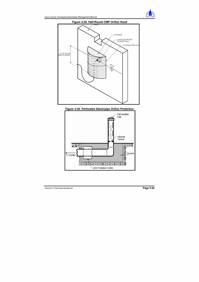
8/11/2019 Vol2 Chap 3 Stormwater Hydrology
http://slidepdf.com/reader/full/vol2-chap-3-stormwater-hydrology 66/76
Knox County Tennessee Stormwater Management Manual
Volume 2 (Technical Guidance) Page 3-66
Figure 3-29. Half-Round CMP Orifice Hood
Figure 3-30. Perforated Stand-pipe Orifice Protection

8/11/2019 Vol2 Chap 3 Stormwater Hydrology
http://slidepdf.com/reader/full/vol2-chap-3-stormwater-hydrology 67/76
Knox County Tennessee Stormwater Management Manual
Volume 2 (Technical Guidance) Page 3-67
3.3.4 Multi-Stage Outlet Design
A combination outlet such as a multiple orifice plate system or multi-stage riser is often used toprovide adequate hydraulic outlet controls for the different design requirements (e.g., WQv, CPv,Qp 2, Qp 10 , Qp 25 and Qp 100 ) for stormwater ponds, stormwater wetlands and detention-only facilities.Separate openings or devices at different elevations are used to control the rate of discharge from
a facility during multiple design storms. Figure 3-26 (shown previously) is an example of multi-stage combination outlet systems.
A design engineer may be creative to provide the most economical and hydraulically efficient outletdesign possible in designing a multi-stage outlet. Many iterative routings are usually required toarrive at a minimum structure size and storage volume that provides proper control. The stage-discharge table or rating curve is a composite (previously shown in Figure 3-25) of the differentoutlets that are used for different elevations within the multi-stage riser.
3.3.4.1 Multi-Stage Outlet Design Procedure
Below are the steps for designing a multi-stage outlet. Note that if a structural control facility willnot control one or more of the required storage volumes (WQv, CPv, Qp 2, Qp 10 , Qp 25 , and Qp 100 ),then that step in the procedure is skipped.
1. Determine Stormwater Control Volumes. Using the procedures from Sections 3.1 and 3.2,estimate the required storage volumes for water quality treatment (WQv), channel protection(CPv), and overbank flood control (Qp 2, Qp 10 , Qp 25) and extreme flood control (Qp 100 ).
2. Develop Stage-Storage Curve. Using the site geometry and topography, develop the stage-storage curve for the facility in order to provide sufficient storage for the control volumesinvolved in the design.
3. Design the Water Quality Volume Outlet. Design the water quality orifice. If a permanent poolis incorporated into the design of the facility, a portion of the storage volume for water qualitywill be above the elevation of the permanent pool. The outlet can be protected using either areverse slope pipe, a hooded protection device, or another acceptable method.
4. Design the Channel Protection Volume Outlet. Design the stream channel protection extendeddetention outlet (CPv-ED) using either Method 1 or 2 from subsection 3.3.3. For this design,the storage needed for channel protection will be “stacked” on top of the water quality volumestorage elevation determined in Step 3. The total stage-discharge rating curve at this point willinclude the water quality control orifice and the outlet used for stream channel protection. Theoutlet should be protected in a manner similar to that for the water quality orifice.
5. Design Overbank Flood Protection Outlet. The overbank protection volume is added above thewater quality and channel protection storage. Establish the Qp 2, Qp 10 , Qp 25 maximum watersurface elevations using the stage-storage curve and subtract the CPv elevation to find the2-year, 10-year and 25-year maximum head. Select an outlet type and calculate the initial sizeand geometry based upon maintaining the pre-development 2-year, 10-year and 25-year peakdischarge rates. Develop a stage-discharge curve for the combined set of outlets (WQv, CPvand Qp 2, Qp 10 , Qp 25). This procedure is repeated for control (peak flow attenuation) of the
100-year storm (Qp 100 ).6. Check Performance of the Outlet Structure. Perform a hydraulic analysis of the multi-stage
outlet structure using reservoir routing to ensure that all outlets will function as designed.Several iterations may be required to calibrate and optimize the hydraulics and outlets that areused. Also, the structure should operate without excessive surging, noise, vibration, or vortexaction at any stage. This usually requires that the structure have a larger cross-sectional areathan the outlet conduit. The hydraulic analysis of the design must take into account thehydraulic changes that will occur as depth of storage changes for the different design storms.As shown in Figure 3-31, as the water passes over the rim of a riser, the riser acts as a weir.However, when the water surface reaches a certain height over the rim of a riser, the riser willbegin to act as a submerged orifice. The designer must compute the elevation at which this

8/11/2019 Vol2 Chap 3 Stormwater Hydrology
http://slidepdf.com/reader/full/vol2-chap-3-stormwater-hydrology 68/76
Knox County Tennessee Stormwater Management Manual
Volume 2 (Technical Guidance) Page 3-68
transition from riser weir flow control to riser orifice flow control takes place for an outlet wherethis change in hydraulic conditions will occur. Also note in Figure 3-31 that as the elevation ofthe water increases further, the control can change from barrel inlet flow control to barrel pipeflow control. Figure 3-32 shows another condition where weir flow can change to orifice flow,which must be taken into account in the hydraulics of the rating curve as different designconditions result in changing water surface elevations.
Figure 3-31. Riser Flow Diagrams(Source: Virginia Department of Conservation and Recreation, 1999)
Figure 3-32. Weir and Orifice Flow(Source: Virginia Department of Conservation and Recreation, 1999)

8/11/2019 Vol2 Chap 3 Stormwater Hydrology
http://slidepdf.com/reader/full/vol2-chap-3-stormwater-hydrology 69/76
Knox County Tennessee Stormwater Management Manual
Volume 2 (Technical Guidance) Page 3-69
7. Size the Emergency Spillway. It is recommended that all stormwater impoundment structureshave a vegetated emergency spillway. An emergency spillway provides a degree of safety toprevent overtopping of an embankment if the primary outlet or principal spillway shouldbecome clogged, or otherwise inoperative. The 100-year storm should be routed through theoutlet devices and emergency spillway to ensure the hydraulics of the system will operate asdesigned.
8. Design Outlet Protection. Design necessary outlet protection and energy dissipation facilitiesto avoid erosion problems downstream from outlet devices and emergency spillway(s). Referto Chapter 7 for more information.
9. Perform Buoyancy Calculations. Perform buoyancy calculations for the outlet structure andfooting. Flotation will occur when the weight of the structure is less than or equal to thebuoyant force exerted by the water.
10. Provide Seepage Control. Seepage control should be provided for the outflow pipe or culvertthrough an embankment. The two most common devices for controlling seepage are (1) filterand drainage diaphragms and (2) anti-seep collars.
3.3.5 Trash Racks and Safety Grates
The susceptibility of larger inlets to clogging by debris and trash needs to be considered whenestimating their hydraulic capacities. In most instances, trash racks will be needed. Trash racksand safety grates are a critical element of outlet structure design and serve several importantfunctions. When properly designed, installed, and maintained, trash racks:
• keep debris away from the entrance to the outlet works where the debris will not clog thecritical portions of the structure;
• capture debris in such a way that relatively easy removal is possible;
• ensure that people and large animals are kept out of confined conveyance and outlet areas;and,
• provide a safety system that prevents humans and animals from being drawn into the outletand allows them to climb to safety.
Trash racks can serve these purposes without interfering significantly with the hydraulic capacity ofthe outlet (or inlet in the case of conveyance structures) (ASCE, 1985; Allred-Coonrod, 1991). Thelocation and size of the trash rack depends on a number of factors, including head losses throughthe rack, structural convenience, safety and size of outlet.
3.3.5.1 Trash Rack DesignAn example of trash racks used on a riser outlet structure is shown in Figure 3-33. The inclinedvertical bar rack is most effective for lower stage outlets. Debris will ride up the trash rack as waterlevels rise. This design also allows for removal of accumulated debris with a rake while standingon top of the structure.
Trash racks must be large enough such that partial plugging will not adversely restrict flowsreaching the control outlet. There are no universal guidelines for the design of trash racks toprotect detention basin outlets, although a commonly used "rule-of-thumb" is to have the trash rackarea at least ten times larger than the control outlet orifice.
The surface area of all trash racks should be maximized and the trash racks should be located asuitable distance from the protected outlet to avoid interference with the hydraulic capacity of theoutlet. The spacing of trash rack bars must be proportioned to the size of the smallest outletprotected. However, where a small orifice is provided, a separate trash rack for that outlet shouldbe used, so that a simpler, sturdier trash rack with more widely spaced members can be used for

8/11/2019 Vol2 Chap 3 Stormwater Hydrology
http://slidepdf.com/reader/full/vol2-chap-3-stormwater-hydrology 70/76
Knox County Tennessee Stormwater Management Manual
Volume 2 (Technical Guidance) Page 3-70
the other outlets. Spacing of the rack bars should be wide enough to avoid interference, but closeenough to provide the level of clogging protection required.
Figure 3-33. Trash Racks Used on a Riser Outlet Structure(Source: Virginia Department of Conservation and Recreation, 1999)
To facilitate removal of accumulated debris and sediment from around the outlet structure, theracks should have hinged connections. If the rack is bolted or set in concrete it will precluderemoval of accumulated material and will eventually adversely affect the outlet hydraulics.
Since sediment will tend to accumulate around the lowest stage outlet, the inside of the outletstructure for a dry basin should be depressed below the ground level to minimize clogging due tosedimentation. Depressing the outlet bottom to a depth below the ground surface at least equal tothe diameter of the outlet is recommended.
Trash racks at entrances to pipes and conduits should be sloped at about 3H:1V to 5H:1V to allowtrash to slide up the rack with flow pressure and rising water level—the slower the approach offlow, the flatter the trash rack angle. Rack opening rules-of-thumb are found in literature. Figure3-34 gives opening estimates based on outlet diameter (Urban Drainage and Flood Control District,1999). Judgment should be used in that an area with higher debris (e.g., a wooded area) mayrequire more opening space.

8/11/2019 Vol2 Chap 3 Stormwater Hydrology
http://slidepdf.com/reader/full/vol2-chap-3-stormwater-hydrology 71/76
Knox County Tennessee Stormwater Management Manual
Volume 2 (Technical Guidance) Page 3-71
Figure 3-34. Minimum Rack Size vs. Outlet Diameter(Source: Urban Drainage and Flood Control District, 1999)
The bar opening space for small pipes should be less than the pipe diameter. For larger diameterpipes, openings should be 6 inches or less. Collapsible racks have been used in some places ifclogging becomes excessive or a person becomes pinned to the rack. Alternately, debris for
culvert openings can be caught upstream from the opening by using pipes placed in the ground ora chain safety net (United States Bureau of Reclamation, 1978; Urban Drainage and Flood ControlDistrict, 1999). Racks can be hinged on top to allow for easy opening and cleaning.
The control for the outlet should not shift to the grate, nor should the grate cause the headwater torise above planned levels. Therefore, head losses through the grate should be calculated. Anumber of empirical loss equations exist though many have difficult to estimate variables. Two willbe given to allow for comparison.
Equation 3-49 can be used to determine the head loss through a trash rack (Metcalf and Eddy,1972). In the use of Equation 3-49, grate openings should be calculated assuming a certainpercentage blockage as a worst case to determine losses and upstream head. Often 40 to 50%blockage is chosen as a working assumption.
Equation 3-49 gu
gg gV
xw
K H θ sin2
234
1
=
where:Hg = head loss through grate (ft)Kg1 = bar shape factor:
2.42 – sharp-edged rectangular1.83 - rectangular bars with semicircular upstream faces1.79 - circular bars1.67 - rectangular bars with semicircular up- and downstream faces

8/11/2019 Vol2 Chap 3 Stormwater Hydrology
http://slidepdf.com/reader/full/vol2-chap-3-stormwater-hydrology 72/76
Knox County Tennessee Stormwater Management Manual
Volume 2 (Technical Guidance) Page 3-72
w = maximum cross-sectional bar width facing the flow (in)x = minimum clear spacing between bars (in)Vu = approach velocity (ft/s)θ g = angle of the grate with respect to the horizontal (degrees)g = acceleration of gravity (32.2 ft/s 2)
The United States Army Corps of Engineers has developed a similar head loss equation for trashracks, shown in Equation 3-50 (USACE, 1988). This equation is for vertical racks, but presumablycan be adjusted through multiplication by the sine of the angle of the grate with respect to thehorizontal, in a manner similar to the previous equation.
Equation 3-50g
V K H ug
g 2
22=
where:
Hg = head loss through grate (ft)Kg2 = defined as described belowVu = approach velocity (ft/s)
g = acceleration of gravity (32.2 ft/s2
)
Kg2 is defined from a series of fit curves, as shown in Table 3-24.
Table 3-24. Fit Curves to Determine K g2
Grate Type Length/thickness CurveSharp-edged rectangular 10 K g2 = 0.00158 - 0.03217 A r + 7.1786 A r
2 Sharp-edged rectangular 5 K g2 = -0.00731 + 0.69453 A r + 7.0856 A r
2 Round edged rectangular 10.9 K g2 = -0.00101 + 0.02520 A r + 6.0000 A r
2 Circular cross-section not applicable K g2 = 0.00866 + 0.13589 A r + 6.0357 A r
2
3.3.6 Secondary OutletsThe purpose of a secondary outlet (emergency spillway) is to provide a controlled overflow forflows in excess of the maximum design storm for a storage facility. Figure 3-35 shows an exampleof an emergency spillway.
In many cases, on-site stormwater storage facilities do not warrant elaborate studies to determinespillway capacity. While the risk of damage due to failure is a real one, it normally does notapproach the catastrophic risk involved in the overtopping or breaching of a major reservoir. Bycontrast, regional facilities with homes immediately downstream could pose a significant hazard iffailure were to occur, in which case emergency spillway considerations are a major design factor.
3.3.6.1 Emergency Spillway DesignEmergency spillway designs are open channels, usually trapezoidal in cross section, and consist ofan inlet channel, a control section, and an exit channel (see Figure 3-35). The emergency spillwayis proportioned to pass flows in excess of the 100-year flood without allowing excessive velocitiesand without overtopping of the embankment. Flow in the emergency spillway is open channel flow.Normally, it is assumed that critical depth occurs at the control section. Volume 2, Chapter 7provides more information on open channel hydraulics.
SCS manuals provide guidance for the selection of emergency spillway characteristics for differentsoil conditions and different types of vegetation. The selection of degree of retardance for a givenspillway depends on the vegetation. Knowing the retardance factor and the estimated dischargerate, the emergency spillway bottom width can be determined. For erosion protection during thefirst year, assume minimum retardance. Both the inlet and exit channels should have a straight

8/11/2019 Vol2 Chap 3 Stormwater Hydrology
http://slidepdf.com/reader/full/vol2-chap-3-stormwater-hydrology 73/76
Knox County Tennessee Stormwater Management Manual
Volume 2 (Technical Guidance) Page 3-73
alignment and grade. Spillway side slopes should be no steeper the 3:1 (horizontal to vertical).The most common type of emergency spillway used is a broad-crested overflow weir cut throughoriginal ground next to the embankment. The transverse cross section of the weir cut is typicallytrapezoidal in shape for ease of construction. Such an excavated emergency spillway is illustratedbelow.
Figure 3-35. Emergency Spillway (Source: Virginia Department of Conservation and Recreation, 1999)

8/11/2019 Vol2 Chap 3 Stormwater Hydrology
http://slidepdf.com/reader/full/vol2-chap-3-stormwater-hydrology 74/76

8/11/2019 Vol2 Chap 3 Stormwater Hydrology
http://slidepdf.com/reader/full/vol2-chap-3-stormwater-hydrology 75/76

8/11/2019 Vol2 Chap 3 Stormwater Hydrology
http://slidepdf.com/reader/full/vol2-chap-3-stormwater-hydrology 76/76
Knox County Tennessee Stormwater Management Manual
This page left intentionally blank.