Printed by Karunaratne & Sons (Pvt) Ltd.

Vol. XXXXIV, No. 03, July 2011

ENGINEER JOURNAL OF THE INSTITUTION OF ENGINEERS, SRI LANKA

EDITORIAL BOARD Eng. (Prof.) A. K. W. Jayawardane Eng. Priyal De Silva Eng. W. T. R. De Silva Eng. (Prof.) K. P. P. Pathirana - Editor Transactions Eng. (Prof.) T. M. Pallewatta - Editor “ENGINEER” Eng. (Dr.) D. A. R. Dolage Eng. (Miss.) Arundathi Wimalasuriya Eng. M. L. Weerasinghe - Editor “SLEN” Eng. (Dr.) K. S. Wanniarachchi Eng. (Prof.) S. S. L. Hettiarachchi The Institution of Engineers, Sri Lanka 120/15, Wijerama Mawatha, Colombo - 00700 Sri Lanka. Telephone: 94-11-2698426, 2685490, 2699210 Fax: 94-11-2699202 E-mail: iesl@slt.lk E-mail (Publications): ed@sltnet.lk Website: http://www.iesl.lk

COVER PAGE

Kokavil Tower Kokavil tower, the main component of the Multi - functional Communication Transmission Center, was commissioned on the 6th June 2011, stands as the tallest tower in Sri Lanka. At a total height of 174 m, this tower is further distinguished as the tallest free standing tower in South Asia. The new Kokavil Tower, constructed under the auspices of the Uthuru Wasanthaya Programme, is located at the site of the previous tower which was destroyed by the terrorists. The center built under the direction of the Telecommunications Regulatory Commission of Sri Lanka was constructed at a cost of Rs. 310 million, by the Central Engineering Consultancy Bureau on a Design and Built Contract Basis. This Transmission Tower will be of great help in alleviating problems associated with telecommunication, television, radio and ICT, affecting the communities in the Northern Sri Lanka. Courtesy of: Eng. Dharmasiri De Alwis, Head of Projects of TRCSL

CONTENTS

Vol.: XXXXIV, No. 03, July 2011 ISSN 1800-1122

From the Editor ... III

SECTION I

Identification of the Spatial Variability of 1 Runoff Coefficients of Three Wet Zone Watersheds of Sri Lanka by : Eng. (Dr.) (Mrs) K. R. J. Perera and Eng. (Prof.) N. T. S. Wijesekara

The following Paper was placed in the First ‘Over 35 years of age’ Category at the Competition on “Infrastructure for Sustainable Development of Water and Other Natural Resources” 2009/2010.

Preparation of the Stormwater Drainage 11 Management Plan for Matara Municipal Council by : Eng. (Prof.) N. T.S. Wijesekera and Eng. (Dr.) K.M.P.S. Bandara

SECTION II

Impact on Existing Transport Systems by 31 Generated Traffic due to New Developments by : Eng. (Prof.) K. S. Weerasekera Comparison of Performance Assessment 39 Indicators for the Evaluation of Irrigation Development of Sri Lanka by: Eng. S. M. D. L. K. De Alwis and Eng. (Prof.) N. T. S. Wijesekara

Pull-out Behavior of Reinforcing Tendons 51 of Nehemiah Anchored Earth System by: Eng. K. J. S. Munasinghe and Eng. R. D. D. Dayawansha The following Paper was placed in the Second ‘Over 35 years of age’ Category at the Competition on “Infrastructure for Sustainable Development of Water and Other Natural Resources” 2009/2010.

Economic Analysis of Water Infrastructure: 57 Have We Got It Right? By : Eng. (Dr.) (Mrs.) Bhadranie Thoradeniya, Eng. (Prof.) Malik Ranasinghe and Eng. (Prof.) N. T. S. Wijesekara

The statements made or opinions expressed in the “Engineer” do not necessarily reflect the views of the Council or a Committee of the Institution of Engineers Sri Lanka, unless expressly stated.

Notes: ENGINEER, established in 1973, is a Quarterly

Journal, published in the months of January, April, July & October of the year.

All published articles have been refereed in anonymity by at least two subject specialists.

Section I contains articles based on Engineering Research while Section II contains articles of Professional Interest.

Vol. XXXXIV, No. 03, July 2011

III

FROM THE EDITOR………….. Tallest self standing tower in South Asia, a remarkable entity indeed, is the newly commissioned Kokavil multi-functional communication tower. Though Sri Lanka is a small country, we have had more than our fair share of biggest, longest, etc., of things to be proud of. Tallest masonry structure – inclusive of foundation, largest sugar factory, biggest school are some that comes to one’s mind, without much difficulty. So have we got in to the Guinness book of records in no insubstantial manner through deeds as well as icons. Whatever is said and done, we are a nation inspired by record breaking creations and achievements. Coming back to Kokavil tower, our object of discussion, it is heartening to note that the design and construction was carried out by a local semi government Engineering organization – namely Central Engineering Consultancy Bureau. Apart from the record setting height, the project has set another record in safety by completing the tower reaching precarious heights, without a single noteworthy accident. In an era where even the simplest of construction tasks are entrusted to expatriate consultants and constructors, the initiative by the client, the Telecommunications Regulatory Commission and the Government of Sri Lanka, to entrust this extraordinary works to local Engineers is laudable. Further, the pioneering spirit of undertaking such a challenge by the Central Engineering Consultancy Bureau Engineers as a Designed and Built project has to be commended. This project would have undoubtedly imparted them with a wealth of experience and confidence. All in all, the direction indicated by this successful landmark project is the correct path for sustainable national infrastructure development while consolidating the confidence in the professional skills of our Engineers. Eng. (Prof.) T. M. Pallewatta, Int. PEng (SL), C. Eng, FIE(SL), FIAE(SL) Editor, ‘ENGINEER’, Journal of The Institution of Engineers.

SECTION I

1 ENGINEER

ENGINEER - Vol. XXXXIV, No. 03, pp. [1-10], 2011© The Institution of Engineers, Sri Lanka

Identification of the Spatial Variability of Runoff Coefficients of Three Wet Zone Watersheds of Sri

Lanka

K. R. J. Perera and N. T. S. Wijesekera

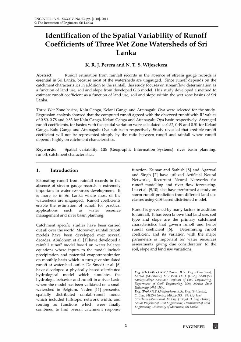
Abstract: Runoff estimation from rainfall records in the absence of stream gauge records is essential in Sri Lanka, because most of the watersheds are ungauged. Since runoff depends on the catchment characteristics in addition to the rainfall, this study focuses on streamflow determination as a function of land use, soil and slope from developed GIS model. This study developed a method to estimate runoff coefficient as a function of land use, soil and slope within the wet zone basins of Sri Lanka. Three Wet Zone basins, Kalu Ganga, Kelani Ganga and Attanagalu Oya were selected for the study. Regression analysis showed that the computed runoff agreed with the observed runoff with R2 values of 0.80, 0.78 and 0.83 for Kalu Ganga, Kelani Ganga and Attanagalu Oya basin respectively. Averaged runoff coefficients, for basins with the spatial variation were calculated as 0.52, 0.49 and 0.51 for Kelani Ganga, Kalu Ganga and Attanagalu Oya sub basin respectively. Study revealed that credible runoff coefficient will not be represented simply by the ratio between runoff and rainfall where runoff depends highly on catchment characteristics. Keywords: Spatial variability, GIS (Geographic Information Systems), river basin planning, runoff, catchment characteristics. 1. Introduction Estimating runoff from rainfall records in the absence of stream gauge records is extremely important in water resources development. It is more so in Sri Lanka where most of the watersheds are ungauged. Runoff coefficients enable the estimation of runoff for practical applications such as water resource management and river basin planning. Catchment specific studies have been carried out all over the world. Moreover, rainfall runoff models have been developed over several decades. Abulohom et al. [1] have developed a rainfall runoff model based on water balance equations where inputs to the model include precipitation and potential evapotranspiration on monthly basis which in turn give simulated runoff at watershed outlet. De Smedt et al. [6] have developed a physically based distributed hydrological model which simulates the hydrologic behavior and runoff in a river basin where the model has been validated on a small watershed in Belgium. Naden [11] presented spatially distributed rainfall-runoff model which included hillslope, network width, and routing as functions which were finally combined to find overall catchment response

function. Kumar and Sathish [8] and Agarwal and Singh [2] have utilized Artificial Neural Networks, Recurrent Neural Networks for runoff modelling and river flow forecasting. Liu et al. [9,10] also have performed a study on storm runoff prediction from different land use classes using GIS-based distributed model. Runoff is governed by many factors in addition to rainfall. It has been known that land use, soil type and slope are the primary catchment characteristics that govern runoff and hence runoff coefficient [6]. Determining runoff coefficient and its variation with the major parameters is important for water resources assessments giving due consideration to the soil, slope and land use variations.

Eng. (Dr.) (Mrs.) K.R.J.Perera, B.Sc. Eng. (Moratuwa), M.Phil. (Moratuwa), MS(USA), Ph.D. (USA), AMIE(Sri Lanka),College Assistant Professor of Civil Engineering, Department of Civil Engineering, New Mexico State University, NM, USA. Eng. (Prof.) N.T.S.Wijesekera, B.Sc. Eng. (Sri Lanka), C. Eng., FIE(Sri Lanka), MICE(UK), PG Dip Hyd Structures (Moratuwa), M. Eng. (Tokyo), D. Eng. (Tokyo). Senior Professor of Civil Engineering, Department of Civil Engineering, University of Moratuwa, Sri Lanka.

ENGINEER 2

#0

#0

$1

Vincit

Karasnagala

-

1 0 10.5Kilometers

$1 Stream Gauge

#0 Rainfall Gauges

Stream Network

Karasnagala Boundary Attanagalu Oya at Kotugoda

Kotugoda

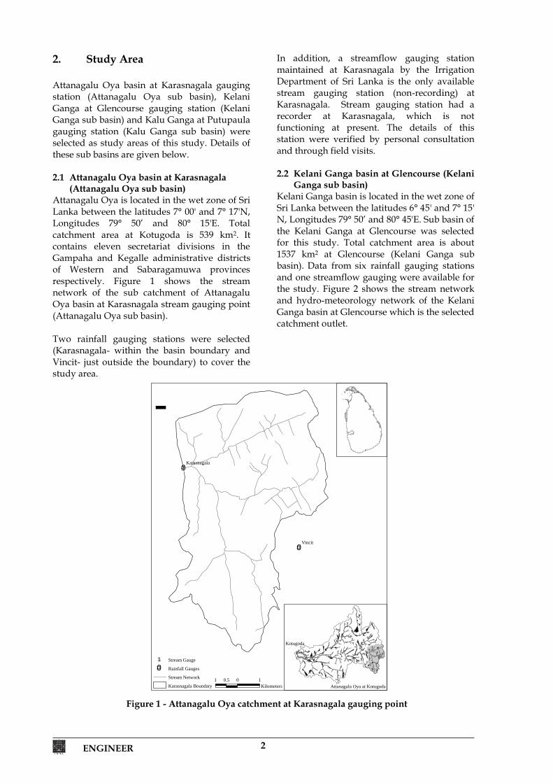
2. Study Area Attanagalu Oya basin at Karasnagala gauging station (Attanagalu Oya sub basin), Kelani Ganga at Glencourse gauging station (Kelani Ganga sub basin) and Kalu Ganga at Putupaula gauging station (Kalu Ganga sub basin) were selected as study areas of this study. Details of these sub basins are given below. 2.1 Attanagalu Oya basin at Karasnagala

(Attanagalu Oya sub basin) Attanagalu Oya is located in the wet zone of Sri Lanka between the latitudes 7° 00' and 7° 17'N, Longitudes 79° 50’ and 80° 15'E. Total catchment area at Kotugoda is 539 km2. It contains eleven secretariat divisions in the Gampaha and Kegalle administrative districts of Western and Sabaragamuwa provinces respectively. Figure 1 shows the stream network of the sub catchment of Attanagalu Oya basin at Karasnagala stream gauging point (Attanagalu Oya sub basin). Two rainfall gauging stations were selected (Karasnagala- within the basin boundary and Vincit- just outside the boundary) to cover the study area.

In addition, a streamflow gauging station maintained at Karasnagala by the Irrigation Department of Sri Lanka is the only available stream gauging station (non-recording) at Karasnagala. Stream gauging station had a recorder at Karasnagala, which is not functioning at present. The details of this station were verified by personal consultation and through field visits. 2.2 Kelani Ganga basin at Glencourse (Kelani

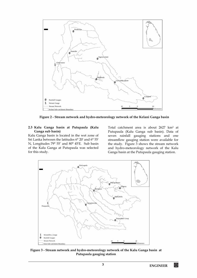
Ganga sub basin) Kelani Ganga basin is located in the wet zone of Sri Lanka between the latitudes 6° 45' and 7° 15' N, Longitudes 79° 50’ and 80° 45'E. Sub basin of the Kelani Ganga at Glencourse was selected for this study. Total catchment area is about 1537 km2 at Glencourse (Kelani Ganga sub basin). Data from six rainfall gauging stations and one streamflow gauging were available for the study. Figure 2 shows the stream network and hydro-meteorology network of the Kelani Ganga basin at Glencourse which is the selected catchment outlet.

Figure 1 - Attanagalu Oya catchment at Karasnagala gauging point

3 ENGINEER

$1

#0

#0

#0

#0#0

#0

Glencourse

Dunedin

Campion

Maliboda

Pindeniya

Ingoya estate

Luccombe estate

-

10 0 105Kilometers

#0 Rainfall Gauges

$1 Stream Gauge

Stream Network

Kelani Sub-catchment Boundary

#0

#0

#0

#0

#0

#0

#0

$1

AlupotaRatnapura

Pelmadulla

Ehelyagoda

Hapugastenna

Gonapinuwala

Dependene Group

-

10 0 105Kilometers

$1 Streamflow_Gauge

#0 Rainfall Gauges

Stream Network

Kalu Sub-catchment Boundary

Putupaulla

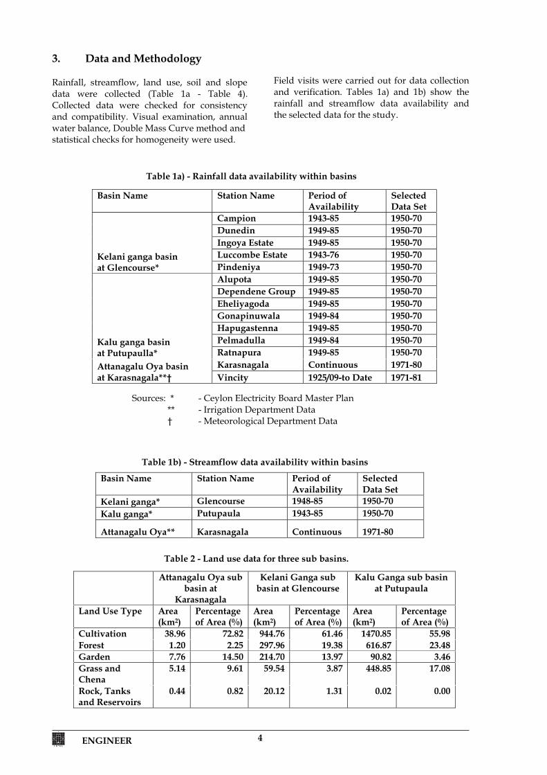
2.3 Kalu Ganga basin at Putupaula (Kalu

Ganga sub basin) Kalu Ganga basin is located in the wet zone of Sri Lanka between the latitudes 6° 20' and 6° 55' N, Longitudes 79° 55’ and 80° 45'E. Sub basin of the Kalu Ganga at Putupaula was selected for this study.

Total catchment area is about 2627 km2 at Putupaula (Kalu Ganga sub basin). Data of seven rainfall gauging stations and one streamflow gauging station were available for the study. Figure 3 shows the stream network and hydro-meteorology network of the Kalu Ganga basin at the Putupaula gauging station.

Figure 2 - Stream network and hydro-meteorology network of the Kelani Ganga basin

Figure 3 - Stream network and hydro-meteorology network of the Kalu Ganga basin at Putupaula gauging station

ENGINEER 4

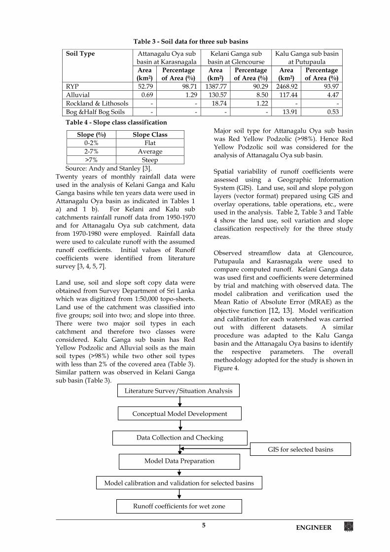
3. Data and Methodology Rainfall, streamflow, land use, soil and slope data were collected (Table 1a - Table 4). Collected data were checked for consistency and compatibility. Visual examination, annual water balance, Double Mass Curve method and statistical checks for homogeneity were used.

Field visits were carried out for data collection and verification. Tables 1a) and 1b) show the rainfall and streamflow data availability and the selected data for the study.

Basin Name Station Name Period of Availability

Selected Data Set

Kelani ganga basin at Glencourse*

Campion 1943-85 1950-70 Dunedin 1949-85 1950-70 Ingoya Estate 1949-85 1950-70 Luccombe Estate 1943-76 1950-70 Pindeniya 1949-73 1950-70

Kalu ganga basin at Putupaulla*

Alupota 1949-85 1950-70 Dependene Group 1949-85 1950-70 Eheliyagoda 1949-85 1950-70 Gonapinuwala 1949-84 1950-70 Hapugastenna 1949-85 1950-70 Pelmadulla 1949-84 1950-70 Ratnapura 1949-85 1950-70

Attanagalu Oya basin at Karasnagala**†

Karasnagala Continuous 1971-80 Vincity 1925/09-to Date 1971-81

Basin Name Station Name Period of Availability

Selected Data Set

Kelani ganga* Glencourse 1948-85 1950-70 Kalu ganga* Putupaula 1943-85 1950-70

Attanagalu Oya** Karasnagala Continuous 1971-80

Attanagalu Oya sub basin at

Karasnagala

Kelani Ganga sub basin at Glencourse

Kalu Ganga sub basin at Putupaula

Land Use Type Area (km2)

Percentage of Area (%)

Area (km2)

Percentage of Area (%)

Area (km2)

Percentage of Area (%)

Cultivation 38.96 72.82 944.76 61.46 1470.85 55.98 Forest 1.20 2.25 297.96 19.38 616.87 23.48 Garden 7.76 14.50 214.70 13.97 90.82 3.46 Grass and Chena

5.14 9.61 59.54 3.87 448.85 17.08

Rock, Tanks and Reservoirs

0.44 0.82 20.12 1.31 0.02 0.00

Table 1a) - Rainfall data availability within basins

Table 1b) - Streamflow data availability within basins

Sources: * - Ceylon Electricity Board Master Plan ** - Irrigation Department Data

† - Meteorological Department Data

Table 2 - Land use data for three sub basins.

5 ENGINEER

Table 4 - Slope class classification

Slope (%) Slope Class 0-2% Flat 2-7% Average >7% Steep

Source: Andy and Stanley [3]. Twenty years of monthly rainfall data were used in the analysis of Kelani Ganga and Kalu Ganga basins while ten years data were used in Attanagalu Oya basin as indicated in Tables 1 a) and 1 b). For Kelani and Kalu sub catchments rainfall runoff data from 1950-1970 and for Attanagalu Oya sub catchment, data from 1970-1980 were employed. Rainfall data were used to calculate runoff with the assumed runoff coefficients. Initial values of Runoff coefficients were identified from literature survey [3, 4, 5, 7]. Land use, soil and slope soft copy data were obtained from Survey Department of Sri Lanka which was digitized from 1:50,000 topo-sheets. Land use of the catchment was classified into five groups; soil into two; and slope into three. There were two major soil types in each catchment and therefore two classes were considered. Kalu Ganga sub basin has Red Yellow Podzolic and Alluvial soils as the main soil types (>98%) while two other soil types with less than 2% of the covered area (Table 3). Similar pattern was observed in Kelani Ganga sub basin (Table 3).

Major soil type for Attanagalu Oya sub basin was Red Yellow Podzolic (>98%). Hence Red Yellow Podzolic soil was considered for the analysis of Attanagalu Oya sub basin. Spatial variability of runoff coefficients were assessed using a Geographic Information System (GIS). Land use, soil and slope polygon layers (vector format) prepared using GIS and overlay operations, table operations, etc., were used in the analysis. Table 2, Table 3 and Table 4 show the land use, soil variation and slope classification respectively for the three study areas. Observed streamflow data at Glencource, Putupaula and Karasnagala were used to compare computed runoff. Kelani Ganga data was used first and coefficients were determined by trial and matching with observed data. The model calibration and verification used the Mean Ratio of Absolute Error (MRAE) as the objective function [12, 13]. Model verification and calibration for each watershed was carried out with different datasets. A similar procedure was adapted to the Kalu Ganga basin and the Attanagalu Oya basins to identify the respective parameters. The overall methodology adopted for the study is shown in Figure 4.

Soil Type Attanagalu Oya sub

basin at Karasnagala Kelani Ganga sub

basin at Glencourse Kalu Ganga sub basin

at Putupaula Area (km2)

Percentage of Area (%)

Area (km2)

Percentage of Area (%)

Area (km2)

Percentage of Area (%)

RYP 52.79 98.71 1387.77 90.29 2468.92 93.97 Alluvial 0.69 1.29 130.57 8.50 117.44 4.47 Rockland & Lithosols - - 18.74 1.22 - - Bog &Half Bog Soils - - - - 13.91 0.53

Table 3 - Soil data for three sub basins

GIS for selected basins

Literature Survey/Situation Analysis

Conceptual Model Development

Data Collection and Checking

Model calibration and validation for selected basins

Runoff coefficients for wet zone

Model Data Preparation

ENGINEER 6

Spatially varied land use, soil and slope data which were collected and identified on maps were digitized using GIS (vector format). Three catchment characteristics for a given basin was overlaid using overlay operation in GIS. This activity creates different land parcels with different catchment characteristics. Required land parcel was selected using table operations for later applications. 3.1 Model development A simple conceptual model was used to compute runoff from each land parcel. The model assumed a linear function incorporating land use, slope and soil as major catchment parameters contributing to convert rainfall into surface runoff.

Surface Runoff = ƒ (Runoff Coefficient, Rainfall)

...(1) The cumulative runoff contributed from each land parcel in a catchment was taken as the surface runoff generated from the catchment. Runoff Coefficient = ƒ (Land use, Slope, Soil)

...(2) Q = (Pijk *Aijk)*R ...(3) where, R = Rainfall Aijk = Area of concern with given factors i,j,k Coefficient Pijk= ƒ (i(1-5), j(1-3), k(1-2))

Table 5 -Land use, slope and soil classification

Land use (i) Slope (j) Soil (k) i Class j Class k Class 1 Forest 1 Flat 1 Red

Yellow Podzolic

2 Garden 2 Average 2 Alluvial 3 Grass &

Chena 3 Steep

4 Cultivation 5 Rocks,

tanks & reservoirs

Pijk represents the coefficient for ith land use type, jth slope class and kth soil type where i varies from 1-5, j varies between 1-3 and k from 1-2. For an instance, P231 represents the coefficient for steep slope garden areas with red yellow podzolic soil type. Parameters of the model assigned by the above criteria are given in Table 6. Model parameters (P values) were estimated (optimized) using Mean Ratio of Absolute Error as the objective function [12, 13]. Parameter optimization was initiated with the literature values [3, 4, 5, 7]. Parameters at which minimum MRAE were selected as finalized parameters of the model. 3.2 Overall runoff coefficient In the present work the overall runoff coefficient which is the area weighted runoff coefficient for a particular watershed was computed using equation 4.

Table 6 - Classification of model parameters on land use, soil and slope

Land Use (i) Slope Class (j)

Soil (k) Red Yellow Podzolic (RYP) - (1)

Alluvial (AL) - (2)

Forest (1)

Flat (0-2 %) (1) (P111) (P112) Average Slope (2-7 %) (2) (P121) (P122) Steep Slope (over 7 %) (3) (P131) (P132)

Garden (2)

Flat (0-2 %) (P211) (P212) Average Slope (2-7 %) (P221) (P222) Steep Slope (over 7 %) (P231) (P232)

Grass & Chena (3)

Flat (0-2 %) (P311) (P312) Average Slope (2-7 %) (P321) (P322) Steep Slope (over 7 %) (P331) (P332)

Cultivation (4)

Flat (0-2 %) (P411) (P412) Average Slope (2-7 %) (P421) (P422) Steep Slope (over 7 %) (P431) (P432)

Rocks, Tanks & Reservoirs (5) Any Slope (P5,1-3,1-2)

7 ENGINEER

This runoff coefficient provides the opportunity to compute an aggregated runoff coefficient for a basin to compute a single runoff coefficient incorporating the variation of soil, slope and land use. Using this method overall runoff coefficients were computed for Kelani, Kalu and Attanagalu Oya basins.

...(4) where, Aijk = Area of concern with given factors i,j,k Coefficient Pijk= ƒ (i(1-5), j(1-3), k(1-2)) and i, j, k are as explained in Table 5. 4. Results and Discussion 4.1 General results for selected watersheds Data checks provided agreeable results with minor error records at Karasnagala streamflow data in year 1975. Annual rainfall for three catchments ranged from 2500mm-5000mm. Typical dry month for the Attanagalu Oya basin is January while for Kelani and Kalu Ganga sub basins, January and February are the dry months. Average rainfall in each basin and runoff data at stream gauging locations of each basin (Karasnagala, Putupaulla and Glencourse for Attanagalu Oya, Kalu Ganga and Kelani Ganga sub basin respectively) were used and calculated the ratio of runoff between rainfall (catchments’ average runoff coefficients). These numbers were found as 0.40, 0.72, and 0.70 for Attanagalu, Kelani and Kalu sub basins respectively. As spatially varied runoff coefficients were found in this study, catchments’ average runoff coefficient were found using the established coefficients as explained in section 3.2.

Hence the runoff coefficients with spatial variation were obtained as 0.51, 0.52, and 0.49 for Attanagalu, Kelani and Kalu sub basins respectively. 4.2 Model parameters and optimized values Each basin contributes to different parameters. Parameters of Kelani Ganga basin were optimized first. Table 7 shows the parameters optimized from Kelani Ganga basin.

The optimized parameters from the Kelani Ganga basin were fixed for the Kalu Ganga basin and the rest of the parameters were optimized for the Kalu Ganga basin which are given in Table 8. Similar analysis was carried out for the Attanagalu Oya basin at Karasnagala and the parameters used and optimized are shown in Table 9. Table 10 shows the finalized coefficients from all three basins, in other words the runoff coefficient matrix. Cultivation contributes higher percentage of land use for all basins. Cultivation includes coconut, rubber, and other cultivation. For the cultivation group optimized runoff coefficients are 0.61, 0.57 and 0.20 for steep, average and flat slopes for red yellow podzolic soils while that for alluvial soils are 0.55 and 0.50 for steep and average slope respectively. Higher amounts of runoff from rainfall was generated in residential areas which was indicated by higher runoff coefficients: 0.65, 0.60, and 0.55 (steep, average and flat slope respectively) for red yellow podzolic soils and 0.56 (steep slope) and 0.52 (average slope) for alluvial soils. Lowest runoff coefficients were obtained for forest areas with alluvial soils (0.10 for steep slope and 0.05 for average slope) followed by red yellow podzolic soils (0.25, 0.20, and 0.10 for steep, average and flat slope respectively).

ijk

ijkijk

AAP

tCoefficienRunoffOverall*

Table 7 - Land use, soil, slope factors considered in the Kelani sub basin and model finalized values

Parameter Optimized Parameter

Land Use Slope Class \ Soil RYP AL RYP AL Forest

Average Slope (2-7 %) Steep Slope (over 7 %) (P131) 0.25

Garden

Average Slope (2-7 %) (P221) (P222) 0.60 0.52 Steep Slope (over 7 %) (P231) (P232) 0.65 0.56

Grass & Chena

Average Slope (2-7 %) Steep Slope (over 7 %) (P331) 0.55

Cultivation

Average Slope (2-7 %) (P421) (P422) 0.57 0.50 Steep Slope (over 7 %) (P431) (P432) 0.61 0.55

Rocks, Tanks, Res. Any Slope (P5,1-3,1-2) 1.00

( (

ENGINEER 8

Table 8 - Land use, soil, slope factors considered in the Kalu Ganga sub basin and finalized values with the model

Parameter Optimized

Parameter Land Use Slope Class \ Soil RYP AL RYP AL

Forest

Average Slope (2-7 %) (P112) (P122) 0.20 0.05 Steep Slope (over 7 %) (P131) (P132) 0.25 0.10

Garden

Average Slope (2-7 %) (P221) (P222) 0.60 0.52 Steep Slope (over 7 %) (P231) (P232) 0.65 0.56

Grass & Chena

Average Slope (2-7 %) (P321) (P322) 0.52 0.35 Steep Slope (over 7 %) (P331) (P332) 0.55 0.40

Cultivation

Average Slope (2-7 %) (P421) (P422) 0.57 0.50 Steep Slope (over 7 %) (P431) (P432) 0.61 0.55

Rocks, Tanks & Res. Any Slope (P5,1-3,1-2) 1.00

Table 9 - Land use, soil, slope factors considered in the Karasnagala sub basin with optimized values

Parameter Optimized

Parameter Land Use Slope Class \ Soil RYP Forest

Flat (0-2 %) (P111) 0.10 Steep Slope (over 7 %) (P131) 0.25

Garden

Flat (0-2 %) (P211) 0.55 Steep Slope (over 7 %) (P231) 0.65

Grass & Chena

Flat (0-2 %) (P311) 0.45 Steep Slope (over 7 %) (P331) 0.55

Cultivation

Flat (0-2 %) (P411) 0.20 Steep Slope (over 7 %) (P431) 0.61

Rocks, Tanks & Res. Any Slope (P5,1-3,1-2) -

Table 10 - Finalized Runoff Coefficient Matrix

Land Use Slope Class \ Soil RYP AL Forest

Flat (0-2 %) 0.10 Average Slope (2-7 %) 0.20 0.05 Steep Slope (over 7 %) 0.25 0.10

Garden

Flat (0-2 %) 0.55 Average Slope (2-7 %) 0.60 0.52 Steep Slope (over 7 %) 0.65 0.56

Grass & Chena

Flat (0-2 %) 0.45 Average Slope (2-7 %) 0.52 0.35 Steep Slope (over 7 %) 0.55 0.40

Cultivation

Flat (0-2 %) 0.20 Average Slope (2-7 %) 0.57 0.50

Steep Slope (over 7 %) 0.61 0.55 Rocks, Tanks & Res. Any Slope 1.00

9 ENGINEER

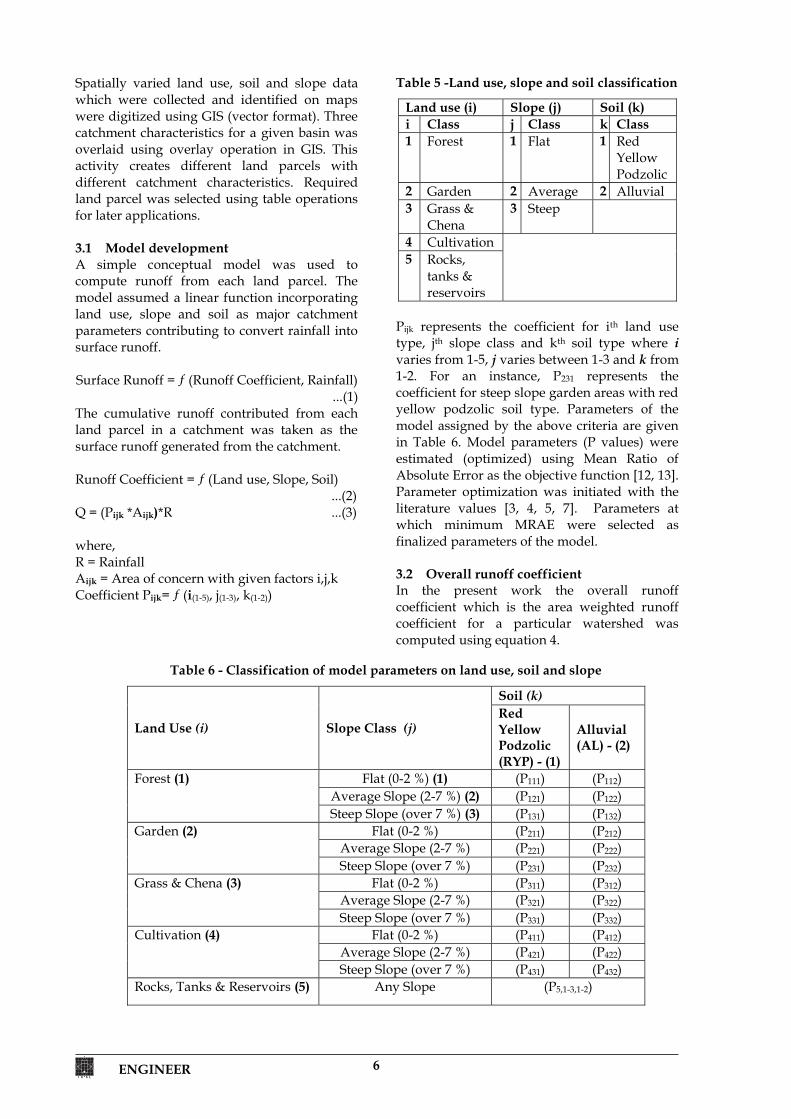
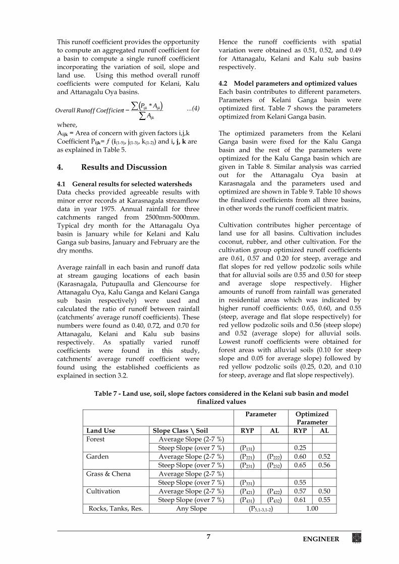
4.3 Calculated vs. observed results The predictive ability of this approach is demonstrated by comparing calculated streamflows against the observed values. Linear regression analysis was carried out with MRAE (objective function) which was used as the measure of the quality of prediction. MRAE of 0.9 and R2 0.83 for Attanagalu Oya sub basin was obtained (Figure 5). For Kelani Ganga sub basin, MRAE was 0.3 and R2 was 0.78 while MRAE for Kalu Ganga sub basin was 0.44 with R2 of 0.80 (Figure 6, Figure 7 respectively). When compared with the objective function, Kelani Ganaga sub basin provided the best fit among three basins. Overall runoff coefficients, for basins with the spatial variation were calculated as 0.52, 0.49 and 0.51 for Kelani, Kalu and Attanagalu sub basins, respectively. Data from five year period (1971-1975) was selected for calibration of Attanagalu Oya sub basin while data from different five years (1976-1980) was used for validation of the model. Figure 5 shows the agreement between modeled and observed streamflow values.

Figure 5 - Calculated Vs observed streamflows for Karasnagala sub basin

The plot in Figure 5 for Attanagalu Oya sub basin (at Karasnagala), indicates an overestimation of the streamflow. As mentioned in methodology and data section, gauging station at Karasnagala was not functioning properly due to clogging by sand where the observed data are undervalued. Figure 6 shows the quality of fit between calculated and observed streamflow values from model calibration (1951-1960) in Kelani

Ganga sub basin. Data from years 1961-1970 was used for model validation. Even though the R2 value is lower compared to the other two basins, best relationship could be observed in Kelani Ganga sub basin data set with low MRAE (Figure 6).

Figure 6 - Calculated Vs observed streamflows for Kelani sub basin

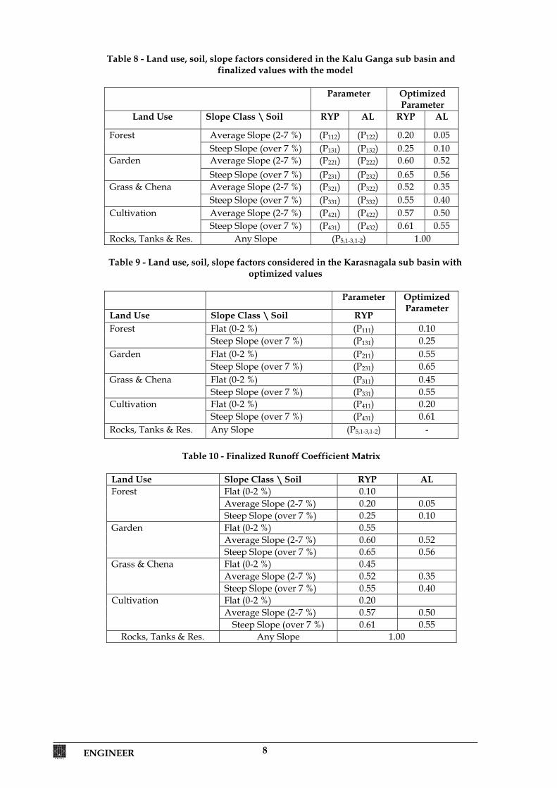
The agreement between the model and the observed streamflow for Kalu Ganga sub basin is shown in Figure 7. Data from 1950-1960 was used for calibration while 1961-1970 used for validation of the model. An underestimation is observed in Kalu Ganga sub basin. Kalu Ganga sub basin land use is cultivation and it receives higher rainfall compared to other two basins of consideration. Overall quality of fit plotted for all three sub basins is shown in Figure 8.

Figure 7 - Calculated Vs observed streamflows

for Kalu Ganga sub basin

ENGINEER 10

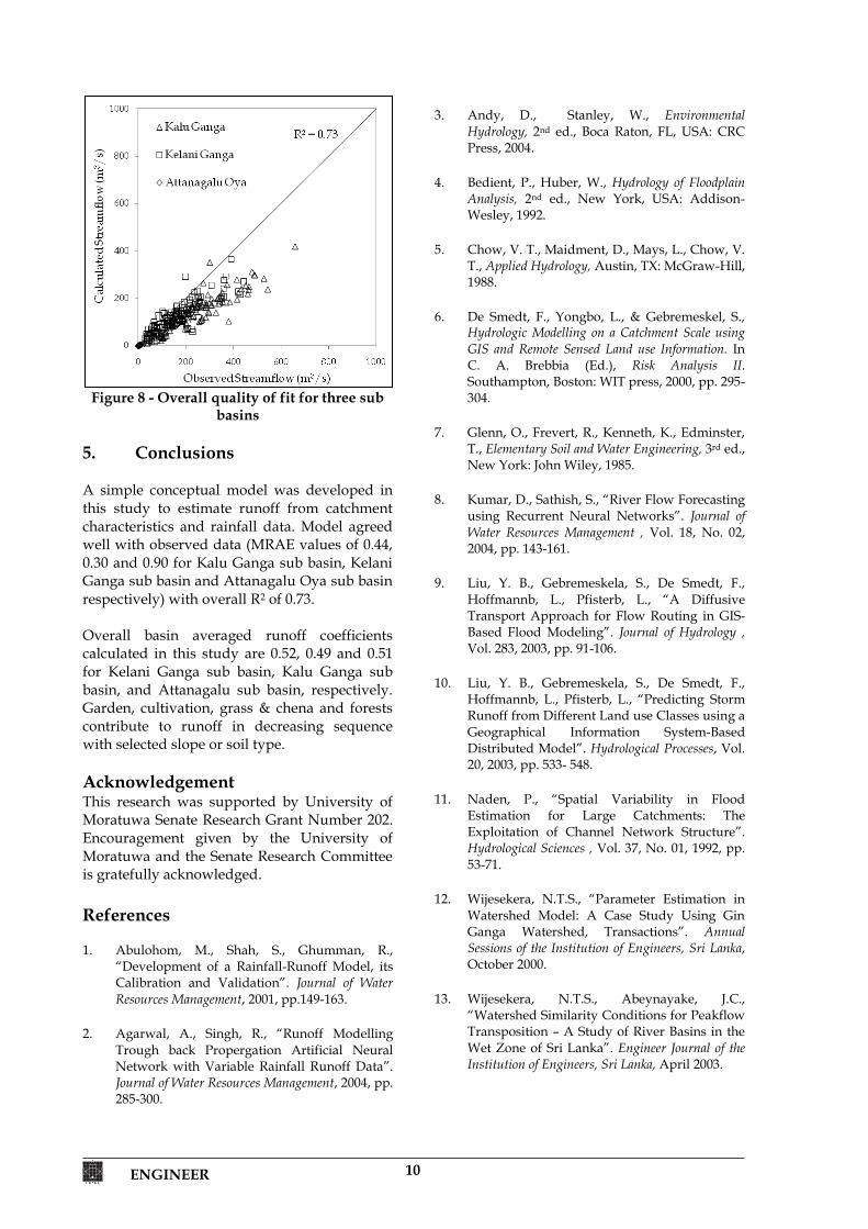
Figure 8 - Overall quality of fit for three sub basins

5. Conclusions A simple conceptual model was developed in this study to estimate runoff from catchment characteristics and rainfall data. Model agreed well with observed data (MRAE values of 0.44, 0.30 and 0.90 for Kalu Ganga sub basin, Kelani Ganga sub basin and Attanagalu Oya sub basin respectively) with overall R2 of 0.73. Overall basin averaged runoff coefficients calculated in this study are 0.52, 0.49 and 0.51 for Kelani Ganga sub basin, Kalu Ganga sub basin, and Attanagalu sub basin, respectively. Garden, cultivation, grass & chena and forests contribute to runoff in decreasing sequence with selected slope or soil type.

Acknowledgement This research was supported by University of Moratuwa Senate Research Grant Number 202. Encouragement given by the University of Moratuwa and the Senate Research Committee is gratefully acknowledged. References 1. Abulohom, M., Shah, S., Ghumman, R.,

“Development of a Rainfall-Runoff Model, its Calibration and Validation”. Journal of Water Resources Management, 2001, pp.149-163.

2. Agarwal, A., Singh, R., “Runoff Modelling

Trough back Propergation Artificial Neural Network with Variable Rainfall Runoff Data”. Journal of Water Resources Management, 2004, pp. 285-300.

3. Andy, D., Stanley, W., Environmental Hydrology, 2nd ed., Boca Raton, FL, USA: CRC Press, 2004.

4. Bedient, P., Huber, W., Hydrology of Floodplain

Analysis, 2nd ed., New York, USA: Addison-Wesley, 1992.

5. Chow, V. T., Maidment, D., Mays, L., Chow, V.

T., Applied Hydrology, Austin, TX: McGraw-Hill, 1988.

6. De Smedt, F., Yongbo, L., & Gebremeskel, S.,

Hydrologic Modelling on a Catchment Scale using GIS and Remote Sensed Land use Information. In C. A. Brebbia (Ed.), Risk Analysis II. Southampton, Boston: WIT press, 2000, pp. 295-304.

7. Glenn, O., Frevert, R., Kenneth, K., Edminster,

T., Elementary Soil and Water Engineering, 3rd ed., New York: John Wiley, 1985.

8. Kumar, D., Sathish, S., “River Flow Forecasting

using Recurrent Neural Networks”. Journal of Water Resources Management , Vol. 18, No. 02, 2004, pp. 143-161.

9. Liu, Y. B., Gebremeskela, S., De Smedt, F.,

Hoffmannb, L., Pfisterb, L., “A Diffusive Transport Approach for Flow Routing in GIS-Based Flood Modeling”. Journal of Hydrology , Vol. 283, 2003, pp. 91-106.

10. Liu, Y. B., Gebremeskela, S., De Smedt, F.,

Hoffmannb, L., Pfisterb, L., “Predicting Storm Runoff from Different Land use Classes using a Geographical Information System-Based Distributed Model”. Hydrological Processes, Vol. 20, 2003, pp. 533- 548.

11. Naden, P., “Spatial Variability in Flood

Estimation for Large Catchments: The Exploitation of Channel Network Structure”. Hydrological Sciences , Vol. 37, No. 01, 1992, pp. 53-71.

12. Wijesekera, N.T.S., “Parameter Estimation in

Watershed Model: A Case Study Using Gin Ganga Watershed, Transactions”. Annual Sessions of the Institution of Engineers, Sri Lanka, October 2000.

13. Wijesekera, N.T.S., Abeynayake, J.C.,

“Watershed Similarity Conditions for Peakflow Transposition – A Study of River Basins in the Wet Zone of Sri Lanka”. Engineer Journal of the Institution of Engineers, Sri Lanka, April 2003.

11 ENGINEER

ENGINEER - Vol. XXXXIV, No. 03, pp. [11-29], 2011© The Institution of Engineers, Sri Lanka

Preparation of the Stormwater Drainage Management Plan for Matara Municipal Council

N.T.S. Wijesekera and K.M.P.S. Bandara

Abstract: Matara Municipal Council area had been experiencing stormwater drainage problems causing inconvenience to public, interruption to work and damage to property. Though the Matara Municipal Council (MMC) had carried out a project in 2001 to develop its drainage canals, there were many cases of flooding within its boundary limits. In order to achieve a suitable plan for stormwater drainage management, the present work carried out an analysis of the associated stormwater drainage system. Systematic field data collection activities were done to identify the flood problem of the area, and to capture sufficient details of terrain and drainages. GPS surveys were conducted to identify the road and drainage alignments. A main feature of the study was the conduct of a road drainage survey which among many other details captured drainage directions along and across the roads. This survey helped to rationally identify the undulations in the terrain to generate the digital terrain model for the generation of stream network and delineation of watersheds. The 1:10,000 elevation data supported by the field work information showed the capability to generate a representative topography for stormwater drainage assessments. Analysis also used a simple Geographic Information System to prioritize critical flood affected areas and enabled identification of critical watersheds for engineering interventions. The present canal system was evaluated with that generated by the model and several sections were identified for early drainage designs these locations were verified in the field. Present work identified that in the MMC area 42% of roads coincide with the stream network indicating a loading of street stormwater drains with runoff generation as a result of terrain changes affected at individual compounds. 164 identified flood locations were analysed with drainage directions and surrounding elevations supported by detailed engineering inspections at specific locations to provide short term solutions. The study made recommendations with respect to development plan approval procedures, preparation of a suitable stormwater drainage database and the need of guidelines for developers to mitigate stormwater drainage problems as part of the long term solutions. Keywords: Urban, Stormwater, Drainage, Management, Terrain Model, GIS, Flood, Field Survey. 1. Introduction Urban areas often experience drainage problems causing flooding to disrupt human activities and leading to numerous environmental problems such as creating mosquito breeding grounds, washing away of garbage to undesirable places, creating stagnant water holes generating unpleasant odour and deteriorating road surfaces. Urban area flooding is usually attributed to new developments blocking the natural waterways, land filling creating changes to drainage directions, filling of flood retention and detention areas, and diversion of natural streams to road side drains etc. In near coast urban centres the low-lying lands also cause drainage problems thereby leading to flood situations when land use changes are conducive to higher runoff generation than that were previously experienced.

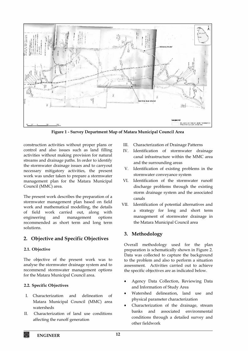
The Matara Municipality Area (Figure 1) had been experiencing stormwater drainage problems causing inconvenience to public, interruption to work and damage to property. The reasons cited for poor stormwater drainage had been given as, the non existence of natural drainage to the sea because most of the lands are either below the sea level or at the same level, many buildings and boundary walls have come up obstructing the natural drainage paths, uncontrolled landfills creating obstacles for flood water flow and storage, lack of proper drainage of stormwater as a result of

Eng. (Prof.) N.T.S. Wijesekera, B.Sc. Eng. Hons, (Sri Lanka), P.G.Dip(Moratuwa), M.Eng.(Tokyo), D.Eng.(Tokyo), C.Eng, FIE(Sri Lanka), MICE(London), Senior Professor of Civil Engineering, Department of Civil Engineering, University of Moratuwa. Eng. (Dr.) K.M.P.S.Bandara, B.Sc.Eng. (Sri Lanka), M.Sc (Geoinformatics-Netherlands), PhD(Netherlands), MBA (Colombo), C.Eng, FIE(Sri Lanka), MICE(London), Director of Engineering Service Board, Ministry of Public Administration & Home Affairs.

ENGINEER 12

construction activities without proper plans or control and also issues such as land filling activities without making provision for natural streams and drainage paths. In order to identify the stormwater drainage issues and to carryout necessary mitigatory activities, the present work was under taken to prepare a stormwater management plan for the Matara Municipal Council (MMC) area. The present work describes the preparation of a stormwater management plan based on field work and mathematical modelling, the details of field work carried out, along with engineering and management options recommended as short term and long term solutions. 2. Objective and Specific Objectives 2.1. Objective The objective of the present work was to analyse the stormwater drainage system and to recommend stormwater management options for the Matara Municipal Council area. 2.2. Specific Objectives

I. Characterization and delineation of

Matara Municipal Council (MMC) area watersheds

II. Characterization of land use conditions affecting the runoff generation

III. Characterization of Drainage Patterns IV. Identification of stormwater drainage

canal infrastructure within the MMC area and the surrounding areas

V. Identification of existing problems in the stormwater conveyance system

VI. Identification of the stormwater runoff discharge problems through the existing storm drainage system and the associated canals

VII. Identification of potential alternatives and a strategy for long and short term management of stormwater drainage in the Matara Municipal Council area

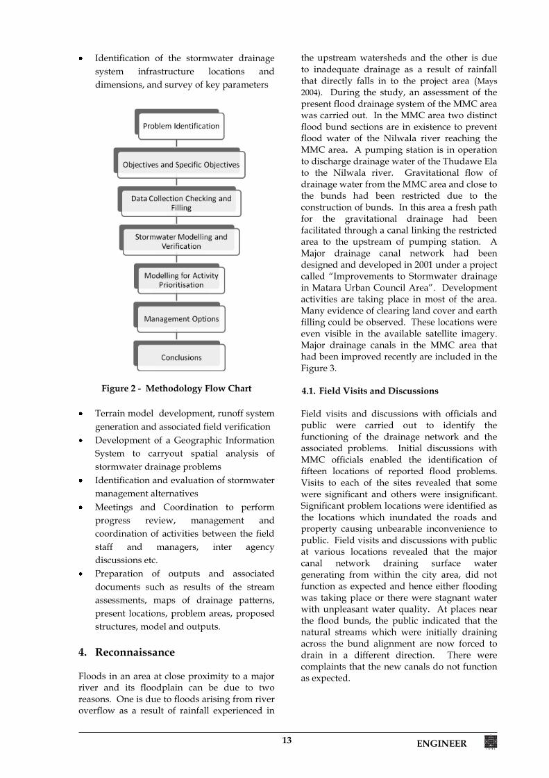
3. Methodology Overall methodology used for the plan preparation is schematically shown in Figure 2. Data was collected to capture the background to the problem and also to perform a situation assessment. Activities carried out to achieve the specific objectives are as indicated below. Agency Data Collection, Reviewing Data

and Information of Study Area Watershed delineation, land use and

physical parameter characterization Characterization of the drainage, stream

banks and associated environmental conditions through a detailed survey and other fieldwork

Figure 1 - Survey Department Map of Matara Municipal Council Area

13 ENGINEER

Identification of the stormwater drainage system infrastructure locations and dimensions, and survey of key parameters

Figure 2 - Methodology Flow Chart

Terrain model development, runoff system

generation and associated field verification Development of a Geographic Information

System to carryout spatial analysis of stormwater drainage problems

Identification and evaluation of stormwater management alternatives

Meetings and Coordination to perform progress review, management and coordination of activities between the field staff and managers, inter agency discussions etc.

Preparation of outputs and associated documents such as results of the stream assessments, maps of drainage patterns, present locations, problem areas, proposed structures, model and outputs.

4. Reconnaissance Floods in an area at close proximity to a major river and its floodplain can be due to two reasons. One is due to floods arising from river overflow as a result of rainfall experienced in

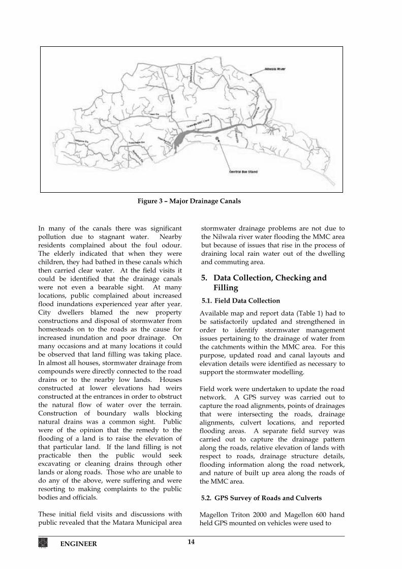
the upstream watersheds and the other is due to inadequate drainage as a result of rainfall that directly falls in to the project area (Mays 2004). During the study, an assessment of the present flood drainage system of the MMC area was carried out. In the MMC area two distinct flood bund sections are in existence to prevent flood water of the Nilwala river reaching the MMC area. A pumping station is in operation to discharge drainage water of the Thudawe Ela to the Nilwala river. Gravitational flow of drainage water from the MMC area and close to the bunds had been restricted due to the construction of bunds. In this area a fresh path for the gravitational drainage had been facilitated through a canal linking the restricted area to the upstream of pumping station. A Major drainage canal network had been designed and developed in 2001 under a project called “Improvements to Stormwater drainage in Matara Urban Council Area”. Development activities are taking place in most of the area. Many evidence of clearing land cover and earth filling could be observed. These locations were even visible in the available satellite imagery. Major drainage canals in the MMC area that had been improved recently are included in the Figure 3. 4.1. Field Visits and Discussions Field visits and discussions with officials and public were carried out to identify the functioning of the drainage network and the associated problems. Initial discussions with MMC officials enabled the identification of fifteen locations of reported flood problems. Visits to each of the sites revealed that some were significant and others were insignificant. Significant problem locations were identified as the locations which inundated the roads and property causing unbearable inconvenience to public. Field visits and discussions with public at various locations revealed that the major canal network draining surface water generating from within the city area, did not function as expected and hence either flooding was taking place or there were stagnant water with unpleasant water quality. At places near the flood bunds, the public indicated that the natural streams which were initially draining across the bund alignment are now forced to drain in a different direction. There were complaints that the new canals do not function as expected.

ENGINEER 14

In many of the canals there was significant pollution due to stagnant water. Nearby residents complained about the foul odour. The elderly indicated that when they were children, they had bathed in these canals which then carried clear water. At the field visits it could be identified that the drainage canals were not even a bearable sight. At many locations, public complained about increased flood inundations experienced year after year. City dwellers blamed the new property constructions and disposal of stormwater from homesteads on to the roads as the cause for increased inundation and poor drainage. On many occasions and at many locations it could be observed that land filling was taking place. In almost all houses, stormwater drainage from compounds were directly connected to the road drains or to the nearby low lands. Houses constructed at lower elevations had weirs constructed at the entrances in order to obstruct the natural flow of water over the terrain. Construction of boundary walls blocking natural drains was a common sight. Public were of the opinion that the remedy to the flooding of a land is to raise the elevation of that particular land. If the land filling is not practicable then the public would seek excavating or cleaning drains through other lands or along roads. Those who are unable to do any of the above, were suffering and were resorting to making complaints to the public bodies and officials. These initial field visits and discussions with public revealed that the Matara Municipal area

stormwater drainage problems are not due to the Nilwala river water flooding the MMC area but because of issues that rise in the process of draining local rain water out of the dwelling and commuting area.

5. Data Collection, Checking and Filling

5.1. Field Data Collection

Available map and report data (Table 1) had to be satisfactorily updated and strengthened in order to identify stormwater management issues pertaining to the drainage of water from the catchments within the MMC area. For this purpose, updated road and canal layouts and elevation details were identified as necessary to support the stormwater modelling. Field work were undertaken to update the road network. A GPS survey was carried out to capture the road alignments, points of drainages that were intersecting the roads, drainage alignments, culvert locations, and reported flooding areas. A separate field survey was carried out to capture the drainage pattern along the roads, relative elevation of lands with respect to roads, drainage structure details, flooding information along the road network, and nature of built up area along the roads of the MMC area. 5.2. GPS Survey of Roads and Culverts Magellon Triton 2000 and Magellon 600 hand held GPS mounted on vehicles were used to

Figure 3 – Major Drainage Canals

15 ENGINEER

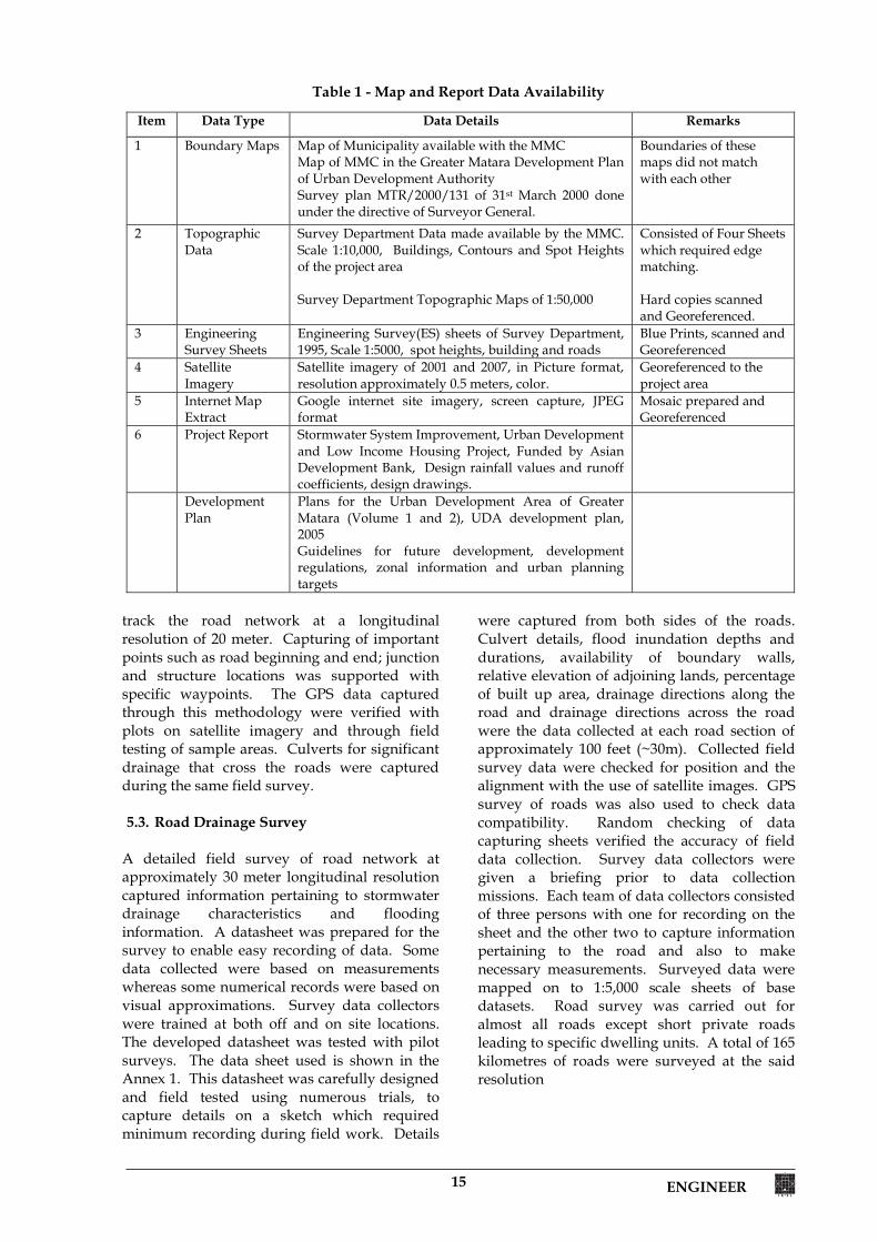
Table 1 - Map and Report Data Availability

track the road network at a longitudinal resolution of 20 meter. Capturing of important points such as road beginning and end; junction and structure locations was supported with specific waypoints. The GPS data captured through this methodology were verified with plots on satellite imagery and through field testing of sample areas. Culverts for significant drainage that cross the roads were captured during the same field survey. 5.3. Road Drainage Survey

A detailed field survey of road network at approximately 30 meter longitudinal resolution captured information pertaining to stormwater drainage characteristics and flooding information. A datasheet was prepared for the survey to enable easy recording of data. Some data collected were based on measurements whereas some numerical records were based on visual approximations. Survey data collectors were trained at both off and on site locations. The developed datasheet was tested with pilot surveys. The data sheet used is shown in the Annex 1. This datasheet was carefully designed and field tested using numerous trials, to capture details on a sketch which required minimum recording during field work. Details

were captured from both sides of the roads. Culvert details, flood inundation depths and durations, availability of boundary walls, relative elevation of adjoining lands, percentage of built up area, drainage directions along the road and drainage directions across the road were the data collected at each road section of approximately 100 feet (~30m). Collected field survey data were checked for position and the alignment with the use of satellite images. GPS survey of roads was also used to check data compatibility. Random checking of data capturing sheets verified the accuracy of field data collection. Survey data collectors were given a briefing prior to data collection missions. Each team of data collectors consisted of three persons with one for recording on the sheet and the other two to capture information pertaining to the road and also to make necessary measurements. Surveyed data were mapped on to 1:5,000 scale sheets of base datasets. Road survey was carried out for almost all roads except short private roads leading to specific dwelling units. A total of 165 kilometres of roads were surveyed at the said resolution

Item Data Type Data Details Remarks

1 Boundary Maps Map of Municipality available with the MMC Map of MMC in the Greater Matara Development Plan of Urban Development Authority Survey plan MTR/2000/131 of 31st March 2000 done under the directive of Surveyor General.

Boundaries of these maps did not match with each other

2 Topographic Data

Survey Department Data made available by the MMC. Scale 1:10,000, Buildings, Contours and Spot Heights of the project area Survey Department Topographic Maps of 1:50,000

Consisted of Four Sheets which required edge matching. Hard copies scanned and Georeferenced.

3 Engineering Survey Sheets

Engineering Survey(ES) sheets of Survey Department, 1995, Scale 1:5000, spot heights, building and roads

Blue Prints, scanned and Georeferenced

4 Satellite Imagery

Satellite imagery of 2001 and 2007, in Picture format, resolution approximately 0.5 meters, color.

Georeferenced to the project area

5 Internet Map Extract

Google internet site imagery, screen capture, JPEG format

Mosaic prepared and Georeferenced

6 Project Report Stormwater System Improvement, Urban Development and Low Income Housing Project, Funded by Asian Development Bank, Design rainfall values and runoff coefficients, design drawings.

Development Plan

Plans for the Urban Development Area of Greater Matara (Volume 1 and 2), UDA development plan, 2005 Guidelines for future development, development regulations, zonal information and urban planning targets

ENGINEER 16

5.4. Drainage Detail and Status Survey A field survey was conducted to capture the locations which had attracted public complaints about poor stormwater drainage. These locations were visited and details were collected including discussions with residents and collection of location photographs. Flood problems were cited with local name of the drainage canals and therefore needed comparison with map data for clarification. A detailed drainage line field survey was conducted to assess the field situation of the drainage canals and to capture other relevant details. 5.5. Data Checking and Filling

All maps were scanned and georeferenced to the Kandawala datum enabling the features to be extracted and were utilized for GIS based computations. Data layers were then printed to a scale of 1:5000 and random field checks of reported information was performed. Data were checked for consistency, and accuracy. In case of elevations when absolute values were not known, a relative comparison of either the data from the same dataset or from different datasets was done to identify disparities. Data showing inconsistency were taken out and wherever possible missing data were given reasonable values considering the surrounding values supported with field visit information. Where the canals had been rehabilitated but the elevations were not available, design gradients in the drawings were used to compute approximate elevations. In cases where canal bank elevations were not available, the ground levels from the topographic maps were taken as the bank elevations. In case elevations of only one bank was available, then the elevations of both banks were considered equal. The drainage and stream alignment were checked closely with the satellite imagery and the traces were adjusted to suit the tracks shown in the satellite imagery. Road traces were also checked, field verified and adjusted in a similar manner. The data checking activity was combined with field visits to ensure data accuracy suitable for computations. 6. Stormwater Modelling

6.1. Terrain Model Development The assessment of stormwater drainage issues requires identifying the geography of the MMC area in sufficient detail and hence a satisfactory digital terrain model of the study area is

required. A terrain model for the assessment of drainage in MMC needs to ensure necessary terrain features for watershed delineation in a flat terrain. Also this terrain model needs to be of sufficiently high resolution to capture the localized flooding issues reported by the public and the Municipality officials. Stormwater generation is highly dependent upon the built up and non-built up area. Therefore it is also necessary to capture the land cover information with adequate representation of the built up area. Accordingly terrain model development was commenced with the use of collected information from maps and reports.

6.1.1. Spatial Resolution In order to model the stormwater drainage in the project area, various spatial resolutions were taken into consideration (Maidment and Djokic 2000). A spatial resolution of 5m was selected by considering the adequacy of details for a management plan, and also considering the computational time required for high resolution data processing (Dutta, Herath and Wijesekera, 2002). Modelling work were also carried out to compare 35m and 50m spatial resolutions and it was noted that such coarse resolutions prevented the reflection of finer details required for stormwater modelling in urban flat terrain.

6.1.2. Elevation Data Adequacy

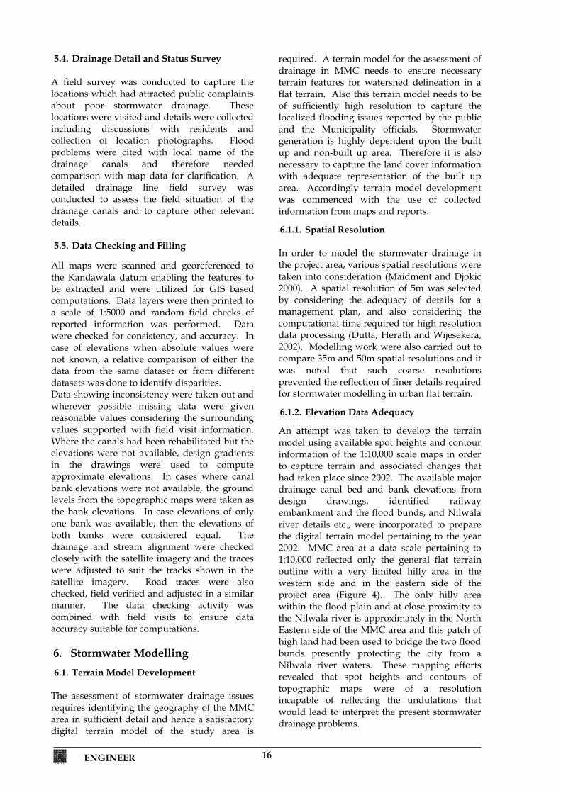
An attempt was taken to develop the terrain model using available spot heights and contour information of the 1:10,000 scale maps in order to capture terrain and associated changes that had taken place since 2002. The available major drainage canal bed and bank elevations from design drawings, identified railway embankment and the flood bunds, and Nilwala river details etc., were incorporated to prepare the digital terrain model pertaining to the year 2002. MMC area at a data scale pertaining to 1:10,000 reflected only the general flat terrain outline with a very limited hilly area in the western side and in the eastern side of the project area (Figure 4). The only hilly area within the flood plain and at close proximity to the Nilwala river is approximately in the North Eastern side of the MMC area and this patch of high land had been used to bridge the two flood bunds presently protecting the city from a Nilwala river waters. These mapping efforts revealed that spot heights and contours of topographic maps were of a resolution incapable of reflecting the undulations that would lead to interpret the present stormwater drainage problems.

17 ENGINEER

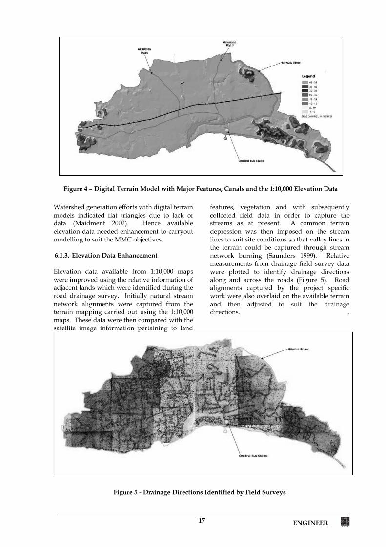
Watershed generation efforts with digital terrain models indicated flat triangles due to lack of data (Maidment 2002). Hence available elevation data needed enhancement to carryout modelling to suit the MMC objectives. 6.1.3. Elevation Data Enhancement Elevation data available from 1:10,000 maps were improved using the relative information of adjacent lands which were identified during the road drainage survey. Initially natural stream network alignments were captured from the terrain mapping carried out using the 1:10,000 maps. These data were then compared with the satellite image information pertaining to land

features, vegetation and with subsequently collected field data in order to capture the streams as at present. A common terrain depression was then imposed on the stream lines to suit site conditions so that valley lines in the terrain could be captured through stream network burning (Saunders 1999). Relative measurements from drainage field survey data were plotted to identify drainage directions along and across the roads (Figure 5). Road alignments captured by the project specific work were also overlaid on the available terrain and then adjusted to suit the drainage directions. .

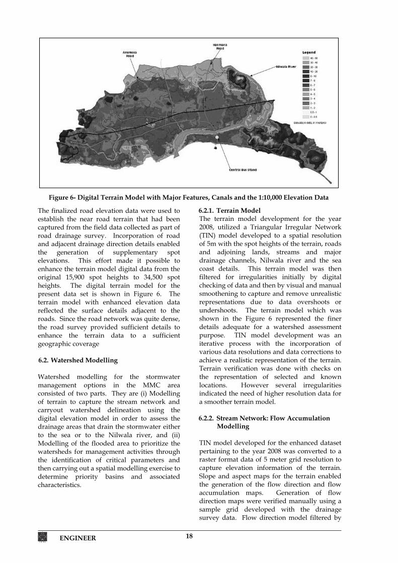
Figure 4 – Digital Terrain Model with Major Features, Canals and the 1:10,000 Elevation Data

Figure 5 - Drainage Directions Identified by Field Surveys

ENGINEER 18

The finalized road elevation data were used to establish the near road terrain that had been captured from the field data collected as part of road drainage survey. Incorporation of road and adjacent drainage direction details enabled the generation of supplementary spot elevations. This effort made it possible to enhance the terrain model digital data from the original 15,900 spot heights to 34,500 spot heights. The digital terrain model for the present data set is shown in Figure 6. The terrain model with enhanced elevation data reflected the surface details adjacent to the roads. Since the road network was quite dense, the road survey provided sufficient details to enhance the terrain data to a sufficient geographic coverage 6.2. Watershed Modelling Watershed modelling for the stormwater management options in the MMC area consisted of two parts. They are (i) Modelling of terrain to capture the stream network and carryout watershed delineation using the digital elevation model in order to assess the drainage areas that drain the stormwater either to the sea or to the Nilwala river, and (ii) Modelling of the flooded area to prioritize the watersheds for management activities through the identification of critical parameters and then carrying out a spatial modelling exercise to determine priority basins and associated characteristics.

6.2.1. Terrain Model The terrain model development for the year 2008, utilized a Triangular Irregular Network (TIN) model developed to a spatial resolution of 5m with the spot heights of the terrain, roads and adjoining lands, streams and major drainage channels, Nilwala river and the sea coast details. This terrain model was then filtered for irregularities initially by digital checking of data and then by visual and manual smoothening to capture and remove unrealistic representations due to data overshoots or undershoots. The terrain model which was shown in the Figure 6 represented the finer details adequate for a watershed assessment purpose. TIN model development was an iterative process with the incorporation of various data resolutions and data corrections to achieve a realistic representation of the terrain. Terrain verification was done with checks on the representation of selected and known locations. However several irregularities indicated the need of higher resolution data for a smoother terrain model. 6.2.2. Stream Network: Flow Accumulation

Modelling TIN model developed for the enhanced dataset pertaining to the year 2008 was converted to a raster format data of 5 meter grid resolution to capture elevation information of the terrain. Slope and aspect maps for the terrain enabled the generation of the flow direction and flow accumulation maps. Generation of flow direction maps were verified manually using a sample grid developed with the drainage survey data. Flow direction model filtered by

Figure 6- Digital Terrain Model with Major Features, Canals and the 1:10,000 Elevation Data

19 ENGINEER

filling the sinks was used to capture the flow accumulation model for the project area. Stream network was delineated with various threshold values for flow accumulation. Trial and error computations indicated that a threshold value of 100 showed the best detailed stream network. Considering the available dataset and while considering the issues pertaining to generating streams in a flat terrain without detailed elevation data, this threshold value presented a highly acceptable stream network map. Streams thus generated were checked for the matching with known terrain and field data. Subsequently the stream network data were compared at selected field locations and was found reliably representative. Field testing locations for the stream network were the flood complaint locations. Stream network generated through the model on most occasions followed the trace of the major drains. However in case of secondary and tertiary drainages, the matching showed a deviation from the terrain depressions that were naturally present in the spot height dataset and also indicated by the vegetation observed in the satellite imagery. The stream network also reflected the drainage direction concerns mentioned by the public. The Nupe Ela and the Kithulampitiya (Weragampita) Canals which were captured from the satellite imagery and rehabilitation plans deviate from the generated ones indicating a different flow direction than that had been anticipated. During field visits and discussion with public verified that the model results are closer to the reality.

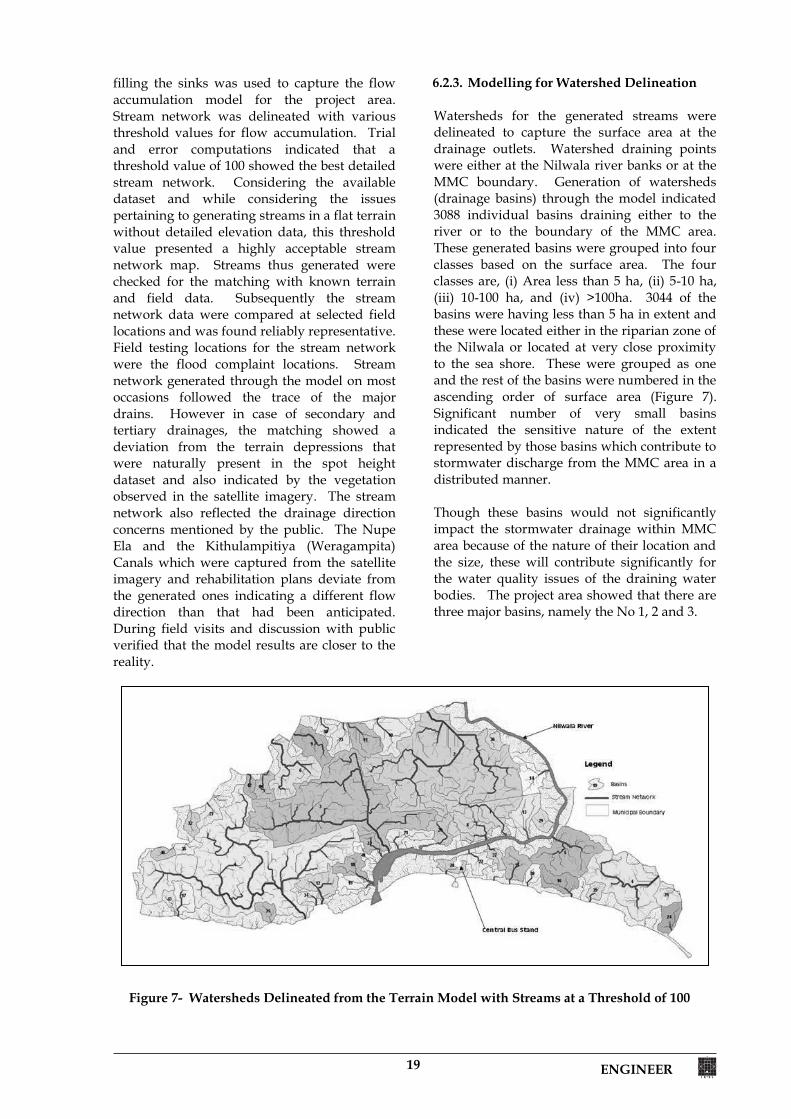
6.2.3. Modelling for Watershed Delineation Watersheds for the generated streams were delineated to capture the surface area at the drainage outlets. Watershed draining points were either at the Nilwala river banks or at the MMC boundary. Generation of watersheds (drainage basins) through the model indicated 3088 individual basins draining either to the river or to the boundary of the MMC area. These generated basins were grouped into four classes based on the surface area. The four classes are, (i) Area less than 5 ha, (ii) 5-10 ha, (iii) 10-100 ha, and (iv) >100ha. 3044 of the basins were having less than 5 ha in extent and these were located either in the riparian zone of the Nilwala or located at very close proximity to the sea shore. These were grouped as one and the rest of the basins were numbered in the ascending order of surface area (Figure 7). Significant number of very small basins indicated the sensitive nature of the extent represented by those basins which contribute to stormwater discharge from the MMC area in a distributed manner. Though these basins would not significantly impact the stormwater drainage within MMC area because of the nature of their location and the size, these will contribute significantly for the water quality issues of the draining water bodies. The project area showed that there are three major basins, namely the No 1, 2 and 3.

Figure 7- Watersheds Delineated from the Terrain Model with Streams at a Threshold of 100

ENGINEER 20

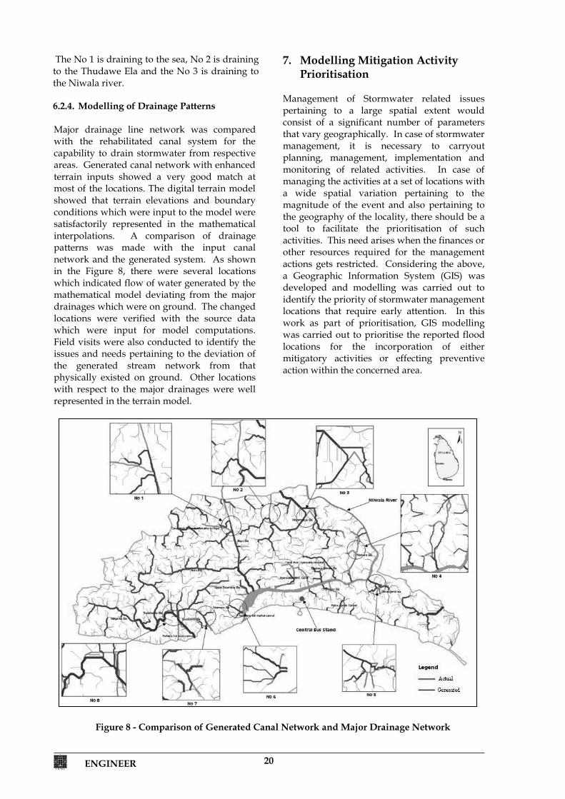
The No 1 is draining to the sea, No 2 is draining to the Thudawe Ela and the No 3 is draining to the Niwala river. 6.2.4. Modelling of Drainage Patterns Major drainage line network was compared with the rehabilitated canal system for the capability to drain stormwater from respective areas. Generated canal network with enhanced terrain inputs showed a very good match at most of the locations. The digital terrain model showed that terrain elevations and boundary conditions which were input to the model were satisfactorily represented in the mathematical interpolations. A comparison of drainage patterns was made with the input canal network and the generated system. As shown in the Figure 8, there were several locations which indicated flow of water generated by the mathematical model deviating from the major drainages which were on ground. The changed locations were verified with the source data which were input for model computations. Field visits were also conducted to identify the issues and needs pertaining to the deviation of the generated stream network from that physically existed on ground. Other locations with respect to the major drainages were well represented in the terrain model.

7. Modelling Mitigation Activity Prioritisation

Management of Stormwater related issues pertaining to a large spatial extent would consist of a significant number of parameters that vary geographically. In case of stormwater management, it is necessary to carryout planning, management, implementation and monitoring of related activities. In case of managing the activities at a set of locations with a wide spatial variation pertaining to the magnitude of the event and also pertaining to the geography of the locality, there should be a tool to facilitate the prioritisation of such activities. This need arises when the finances or other resources required for the management actions gets restricted. Considering the above, a Geographic Information System (GIS) was developed and modelling was carried out to identify the priority of stormwater management locations that require early attention. In this work as part of prioritisation, GIS modelling was carried out to prioritise the reported flood locations for the incorporation of either mitigatory activities or effecting preventive action within the concerned area.

Figure 8 - Comparison of Generated Canal Network and Major Drainage Network

21 ENGINEER

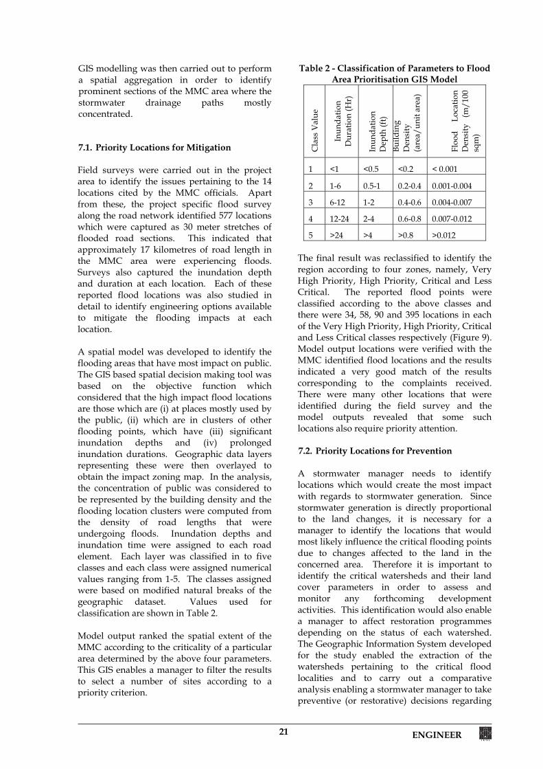
GIS modelling was then carried out to perform a spatial aggregation in order to identify prominent sections of the MMC area where the stormwater drainage paths mostly concentrated. 7.1. Priority Locations for Mitigation Field surveys were carried out in the project area to identify the issues pertaining to the 14 locations cited by the MMC officials. Apart from these, the project specific flood survey along the road network identified 577 locations which were captured as 30 meter stretches of flooded road sections. This indicated that approximately 17 kilometres of road length in the MMC area were experiencing floods. Surveys also captured the inundation depth and duration at each location. Each of these reported flood locations was also studied in detail to identify engineering options available to mitigate the flooding impacts at each location. A spatial model was developed to identify the flooding areas that have most impact on public. The GIS based spatial decision making tool was based on the objective function which considered that the high impact flood locations are those which are (i) at places mostly used by the public, (ii) which are in clusters of other flooding points, which have (iii) significant inundation depths and (iv) prolonged inundation durations. Geographic data layers representing these were then overlayed to obtain the impact zoning map. In the analysis, the concentration of public was considered to be represented by the building density and the flooding location clusters were computed from the density of road lengths that were undergoing floods. Inundation depths and inundation time were assigned to each road element. Each layer was classified in to five classes and each class were assigned numerical values ranging from 1-5. The classes assigned were based on modified natural breaks of the geographic dataset. Values used for classification are shown in Table 2. Model output ranked the spatial extent of the MMC according to the criticality of a particular area determined by the above four parameters. This GIS enables a manager to filter the results to select a number of sites according to a priority criterion.

Table 2 - Classification of Parameters to Flood Area Prioritisation GIS Model

Cla

ss V

alue

Inun

datio

n D

urat

ion

(Hr)

Inun

datio

n D

epth

(ft)

Build

ing

Den

sity

(a

rea/

unit

area

)

Floo

d Lo

catio

n D

ensi

ty

(m/1

00

sqm

)

1 <1 <0.5 <0.2 < 0.001

2 1-6 0.5-1 0.2-0.4 0.001-0.004

3 6-12 1-2 0.4-0.6 0.004-0.007

4 12-24 2-4 0.6-0.8 0.007-0.012

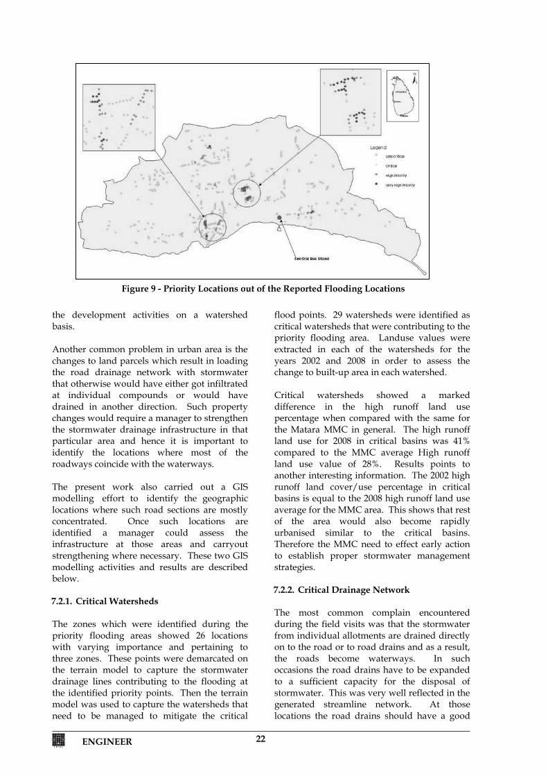
5 >24 >4 >0.8 >0.012 The final result was reclassified to identify the region according to four zones, namely, Very High Priority, High Priority, Critical and Less Critical. The reported flood points were classified according to the above classes and there were 34, 58, 90 and 395 locations in each of the Very High Priority, High Priority, Critical and Less Critical classes respectively (Figure 9). Model output locations were verified with the MMC identified flood locations and the results indicated a very good match of the results corresponding to the complaints received. There were many other locations that were identified during the field survey and the model outputs revealed that some such locations also require priority attention. 7.2. Priority Locations for Prevention A stormwater manager needs to identify locations which would create the most impact with regards to stormwater generation. Since stormwater generation is directly proportional to the land changes, it is necessary for a manager to identify the locations that would most likely influence the critical flooding points due to changes affected to the land in the concerned area. Therefore it is important to identify the critical watersheds and their land cover parameters in order to assess and monitor any forthcoming development activities. This identification would also enable a manager to affect restoration programmes depending on the status of each watershed. The Geographic Information System developed for the study enabled the extraction of the watersheds pertaining to the critical flood localities and to carry out a comparative analysis enabling a stormwater manager to take preventive (or restorative) decisions regarding

ENGINEER 22

the development activities on a watershed basis. Another common problem in urban area is the changes to land parcels which result in loading the road drainage network with stormwater that otherwise would have either got infiltrated at individual compounds or would have drained in another direction. Such property changes would require a manager to strengthen the stormwater drainage infrastructure in that particular area and hence it is important to identify the locations where most of the roadways coincide with the waterways. The present work also carried out a GIS modelling effort to identify the geographic locations where such road sections are mostly concentrated. Once such locations are identified a manager could assess the infrastructure at those areas and carryout strengthening where necessary. These two GIS modelling activities and results are described below. 7.2.1. Critical Watersheds The zones which were identified during the priority flooding areas showed 26 locations with varying importance and pertaining to three zones. These points were demarcated on the terrain model to capture the stormwater drainage lines contributing to the flooding at the identified priority points. Then the terrain model was used to capture the watersheds that need to be managed to mitigate the critical

flood points. 29 watersheds were identified as critical watersheds that were contributing to the priority flooding area. Landuse values were extracted in each of the watersheds for the years 2002 and 2008 in order to assess the change to built-up area in each watershed. Critical watersheds showed a marked difference in the high runoff land use percentage when compared with the same for the Matara MMC in general. The high runoff land use for 2008 in critical basins was 41% compared to the MMC average High runoff land use value of 28%. Results points to another interesting information. The 2002 high runoff land cover/use percentage in critical basins is equal to the 2008 high runoff land use average for the MMC area. This shows that rest of the area would also become rapidly urbanised similar to the critical basins. Therefore the MMC need to effect early action to establish proper stormwater management strategies. 7.2.2. Critical Drainage Network The most common complain encountered during the field visits was that the stormwater from individual allotments are drained directly on to the road or to road drains and as a result, the roads become waterways. In such occasions the road drains have to be expanded to a sufficient capacity for the disposal of stormwater. This was very well reflected in the generated streamline network. At those locations the road drains should have a good

Figure 9 - Priority Locations out of the Reported Flooding Locations

23 ENGINEER

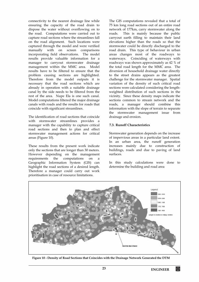
connectivity to the nearest drainage line while ensuring the capacity of the road drain to dispose the water without overflowing on to the road. Computations were carried out to capture road sections where the streamlines fall on the road alignment. Such locations were captured through the model and were verified manually with on screen comparisons incorporating field observations. The model results provide valuable information for a manager to carryout stormwater drainage management within the MMC area. Model results have to be filtered to ensure that the problem causing sections are highlighted. Therefore from the model outputs it is necessary that the road sections which are already in operation with a suitable drainage canal by the side needs to be filtered from the rest of the area. Nupe Ela is one such canal. Model computations filtered the major drainage canals with roads and the results for roads that coincide with significant streamlines. The identification of road sections that coincide with stormwater streamlines provides a manager with the capability to capture critical road sections and then to plan and effect stormwater management actions for critical areas (Figure 10). These results from the present work indicate only the sections that are longer than 30 meters. However depending on the management requirements the computations on a Geographic Information System (GIS) can highlight the road sections of a desired length. Therefore a manager could carry out work prioritisation in case of resource limitations.

The GIS computations revealed that a total of 75 km long road sections out of an entire road network of 177km, carry stormwater along the roads. This is mainly because the public carryout earth filling to maintain their land elevations higher than the roads so that the stormwater could be directly discharged to the road drain. This type of behaviour in urban areas changes most of the roadways to waterways. Coinciding of waterways with roadways was shown approximately as 42 % of the total road length for the MMC area. The diversion of household drainage water directly to the street drains appears as the greatest challenge for the stormwater manager. Spatial variation of the density of such critical road sections were calculated considering the length-weighted distribution of such sections in the vicinity. Since these density maps indicate the sections common to stream network and the roads, a manager should combine this information with the slope of terrain to separate the stormwater management issue from drainage and erosion. 7.3. Runoff Characteristics Stormwater generation depends on the increase of impervious areas in a particular land extent. In an urban area, the runoff generation increases mainly due to construction of buildings, roads and due to paving of land surfaces. In this study calculations were done to determine the building and road area

Figure 10 - Density of Road Sections that Coincides with the Drainage Network Generated the DTM

ENGINEER 24

in the two datasets corresponding to 2002 and 2008. Roads which were in the 1:10,000 scale had subjected to many changes. Roads and Buildings of each year was overlaid on the landuse map of 2002 and each land use type was extracted using the Geographic Information System. These land use categories were then classified into two broad groups as high runoff generating and low runoff generating. Watersheds in general showed an increase in the impervious land cover indicating a high runoff land use percentage of approximately 28% as against a value of 17% for high runoff land cover corresponding to the year 2002. The land use changes of watersheds incorporating average runoff coefficients of 0.7 and 0.25 for high runoff generating and low runoff generating land uses respectively show that the generation of stormwater has increased by 14% from the year 2002 to year 2008. The same computations for a high runoff value of 0.8 and with the same low runoff value of 0.25 would increase the runoff by 16%. 8. Management Recommendations The MMC stormwater drainage system which has many similarities to other urban areas along the coast of Sri Lanka lies on a flat terrain. The main common characteristic is that the public directly discharge stormwater from their properties to the roadway drains. Paved areas in the city are increasing with time due to pressure of dwelling needs in the urban community. The present work of stormwater system analysis indicated the options for stormwater management. The options can be broadly divided into long term and short term. The long term ones would be the preventive actions and good management practices whereas short term ones would be to ease the problems which are presently being experienced. The present work led to the identification of problem areas and goes on to recommend how such areas could be dealt with and also how a manager could determine the areas of priority. 8.1. Short Term Solutions

8.1.1. Major Drainage Lines The mathematical modelling and field work identified that the generated major streams reflected a different behaviour when compared with what had been anticipated during the previous designs and construction. This

indicated that the functioning of the drainage canals at certain points need detailed studies in order to identify the appropriate drainage canal trace, size, slope and other parameters. The stream network generation by the model follows a system which initially identifies the flow directions and then picks up sinks where pools of water results in sets of cells with undetermined flow directions. In the model such pools are filled and then calculations are carried out to identify the flow directions to compute the stream network. An iterative process fills the terrain sinks to produce the final stream network. Stream network generated by the model reflects the functioning of the drainage direction once the pools are filled and hence the direction in which the flood waters would recede. However in reality, when the rains are inadequate then the flow will stop at the sinks creating pools of water. This means that even if the flood is receding there will be pools of water at the locations where the terrain indicate sinks. A close scrutiny of the major canals identified several key issues pertaining to the major canals. Their locations are shown in Figure 8 and descriptions are given thereafter. No.1: In the generated stream network, the Nupe canal is shown as two sections flowing in two directions. A major section is flowing southwards and a smaller section is draining towards the northern boundary. This behaviour shows that even when the surface depressions had been incorporated for the terrain model indicating the presence of a canal, the functioning in reality is different or in other words the flow in the canal is not in one direction. Terrain model has indicated that canal elevation inputs have not supported water flow through the canal alignment. However it is noteworthy that the terrain model represents the behaviour of the canal as described by the officials and the public. Site visits also revealed the presence of a regulator to raise the parent canal head so that the water could flow along the Nupe canal in the direction from North to South. This regulator does not appear to be in operation as at present. Also the recent constructions raising the bed level of the Nupe canal indicates that for the regulator to be useful then the water level would have to be raised to significant elevations. No 2: In the Kithulampitiya canal too there is a section which behaves similarly to Nupe Ela.

25 ENGINEER

The physical inputs show a canal construction but the terrain model shows flow in two separate directions. This indicates the problem when attempting to drain water through the Kithulampitiya canal in the direction of Thudawa. No 3: Kithulampitiya canal is expected to drain water from regions inside the flood bunds at the western edge of the MMC area to the Thudawe Ela at the Northern end. However the model indicates that instead of flowing along the canal trace the drainage flow deviates to lower terrain at a location close to the Mathugala Bund (Wella). Water from the Harischandra properties also drain towards the Mathugama Wella contradicting the flow direction expected from the canal. These behaviour matches with the observations of the public and the complaints made by them indicating that the canal levels need checking because it appears that the canal has been constructed to push the flow in the upstream direction. The terrain model developed for the study has successfully indicated the geographic features that support the drainage of stormwater along this canal system. No 4 at Piladuwa Ela shows two section of the Ela draining in two separate directions while having a ridge close to the railway line. This indicates that the elevations do not permit water to flow along the canal though the ends are linked to form a single canal. The stream network generated by the model clearly reflects the behaviour of the canal system as described by the public during field surveys. At Nos 5,6, 7 and 8 too, the flow directions deviate from the physically excavated canal alignments. This indicates that the terrain does not facilitate the flow directly into the canals which have been rehabilitated. It also means that at the deviations there will be locations of flooding and water collecting pools prior to draining excess water through the stream network as identified by the model. This detailed comparison of model outputs with the physically existing canal system points to the problem locations which are having difficulties in draining stormwater to ensure flood mitigation. Therefore the terrain model output has indicated its strong potential to capture critical locations in the main drainages so that a manager could commence action to pursue detailed engineering studies in the model identified locations to identify the exact

behaviour and then to execute engineering solutions. The generated stream network was categorised according to stream order of tributaries and this enables a manager to initially identify the problem area in the high stream order locations and then to move towards less order streams. In case the terrain details that have been fed to the model are of finer resolution then it is possible to satisfactorily capture the drainage issues even in the level 1 stream order canals. The model has identified locations of incompatibility in the existing drainage system. This enables the stormwater manager to commence action to carryout detailed studies and identify locality specific engineering designs for implementation as indicated above. 8.1.2. Identified Flooding Locations Each of the flooding locations identified during field surveys and at discussions with MMC officials were inspected to identify the best management options. The observations were studied with the terrain model and the generated streamlines to provide options for easing the stormwater drainage problem as at present. Engineering field inspections of the surrounding environment were made at each of the identified flood complaint locations. At most occasions it was identified that either the natural stormwater discharge path had been obstructed by a land or had been over loaded due to large stormwater contributions from surrounding urbanised land. The proposals whilst using site inspection details and satellite imagery recommend the most suitable path for stormwater disposal. However engineering surveys at the recommended vicinity should be carried out prior to construction work. Importantly, long term solutions should be incorporated for each and every critical location to ensure the sustainability of these solutions. Specific solutions were given for the identified 164 locations and a sample is shown in the Figure 11. 8.2. Long Term Solutions 8.2.1. Development Planning and Approval The study identified that the major issue for stormwater management in the long run would be to control the stormwater generation from the urban lands and also to control the simultaneous discharge of the stormwater to the street drainage network. Blockage of natural drainage paths were also identified as a

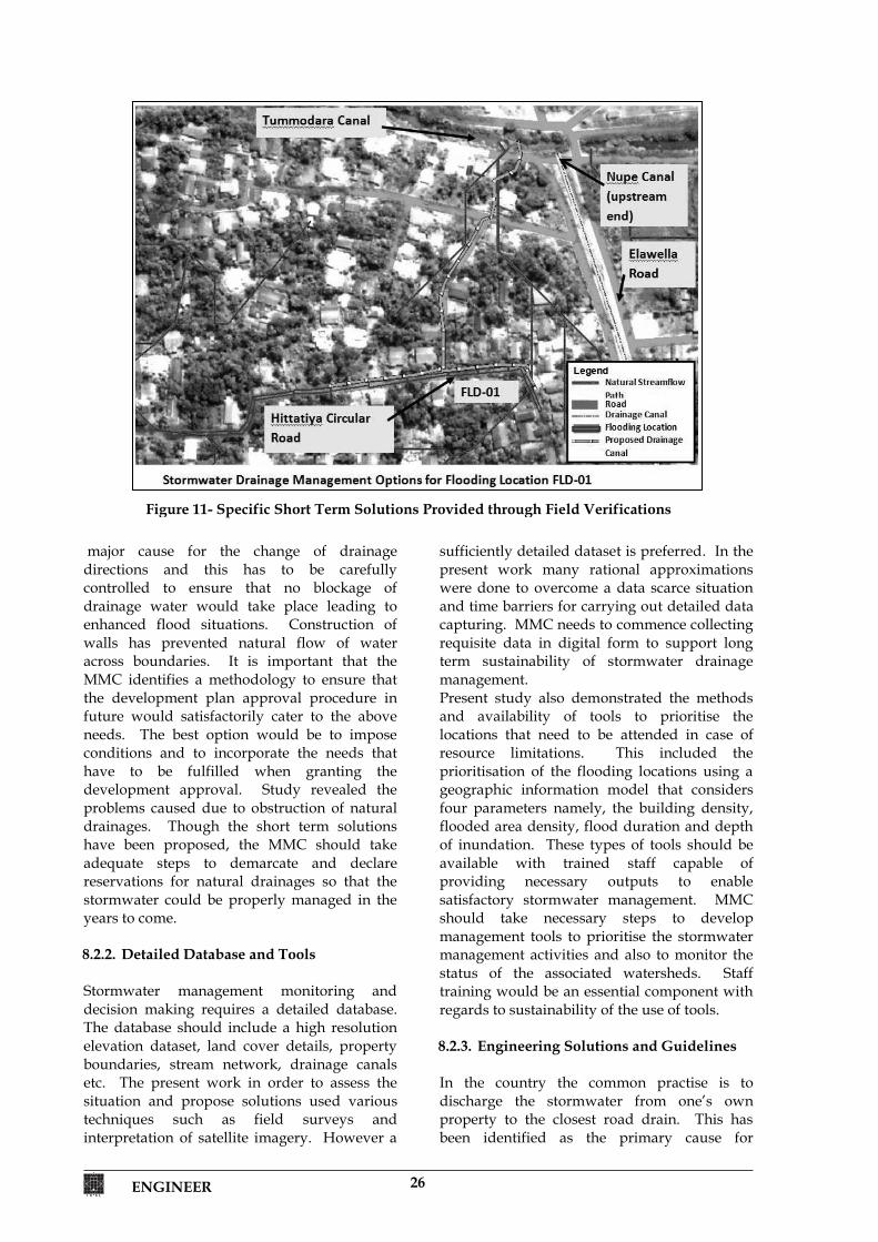
ENGINEER 26

major cause for the change of drainage directions and this has to be carefully controlled to ensure that no blockage of drainage water would take place leading to enhanced flood situations. Construction of walls has prevented natural flow of water across boundaries. It is important that the MMC identifies a methodology to ensure that the development plan approval procedure in future would satisfactorily cater to the above needs. The best option would be to impose conditions and to incorporate the needs that have to be fulfilled when granting the development approval. Study revealed the problems caused due to obstruction of natural drainages. Though the short term solutions have been proposed, the MMC should take adequate steps to demarcate and declare reservations for natural drainages so that the stormwater could be properly managed in the years to come. 8.2.2. Detailed Database and Tools Stormwater management monitoring and decision making requires a detailed database. The database should include a high resolution elevation dataset, land cover details, property boundaries, stream network, drainage canals etc. The present work in order to assess the situation and propose solutions used various techniques such as field surveys and interpretation of satellite imagery. However a

sufficiently detailed dataset is preferred. In the present work many rational approximations were done to overcome a data scarce situation and time barriers for carrying out detailed data capturing. MMC needs to commence collecting requisite data in digital form to support long term sustainability of stormwater drainage management. Present study also demonstrated the methods and availability of tools to prioritise the locations that need to be attended in case of resource limitations. This included the prioritisation of the flooding locations using a geographic information model that considers four parameters namely, the building density, flooded area density, flood duration and depth of inundation. These types of tools should be available with trained staff capable of providing necessary outputs to enable satisfactory stormwater management. MMC should take necessary steps to develop management tools to prioritise the stormwater management activities and also to monitor the status of the associated watersheds. Staff training would be an essential component with regards to sustainability of the use of tools. 8.2.3. Engineering Solutions and Guidelines In the country the common practise is to discharge the stormwater from one’s own property to the closest road drain. This has been identified as the primary cause for

Figure 11- Specific Short Term Solutions Provided through Field Verifications

27 ENGINEER

flooding and especially flash flooding. The MMC needs to ensure that such discharges are carried out within engineering limits imposed by considering the load that can be undertaken by a reasonable drainage infrastructure system. Since the increase of stormwater on the drainage system requires financial inputs to sustain the infrastructure, it may be appropriate for the MMC to consider imposing a levy on those properties that have not constructed stormwater retention or detention facilities. In order to ensure that the public are properly assisted to incorporate stormwater retention and detention, it is necessary that the MMC establishes guidelines for the developers as to what should be constructed, what type and size should be used etc. It is recommended that a handbook for the design and building of such facilities should be made available at the MMC for public use. 9. Conclusions

1. The present study carried out systematic

field and desk studies and clearly identified the long term and short term solutions for rational stormwater management.

2. Watershed delineation efforts for flat terrain requires high resolution elevation data, but in the absence of such survey data, it is possible to use field drainage surveys to create representative digital elevation models using 1:10,000 topographic map elevation data with satellite map interpretations.

3. Simple Geographic Information System incorporating flood inundation level, inundation duration, proximity to populated area, and nearby flood location density enabled the prioritisation of critical locations for management interventions.

4. The present work compared the terrain, the generated stream network, the constructed drainage canals and carried out field inspection of specific locations to successfully propose practically feasible short term solutions for Stormwater drainage management

5. The generated stream network developed for the present situation confirmed that the road drains have become the major drainage water disposal route as a result of landfills and drainage closures. The GIS

enabled the identification of such road section clusters enabling a manager to propose adequate interventions.

6. Eight critical locations in the major drainage network were identified and recommendations were made to ensure proper drainage of stormwater using the existing drainage canal network.

7. Individual flooding locations which were identified during field surveys were grouped in to 164 localities. These locations were inspected, analysed for suitable options, and solutions for proper stormwater disposal have been made while taking efforts to address each individual case and its surroundings.

8. The flood locations identified were spatially modelled using a GIS to identify 34 No of Very High Priority, 58 No of High Priority, and 90 No of Critical flooding locations for implementation of mitigatory action especially in resource limited situations.

9. 29 Critical watersheds pertaining to the priority given to flooding locations were identified with its landuse components facilitating a stormwater manager to monitor and control the development activities in a sustainable manner.

10. A Total of 75 kilometres of road sections which is approximately 42% of the MMC roads, that carry significant stormwater either in its side drains or on the road surface were identified, mapped and prioritised for effecting suitable stormwater management programs.

References 1. Maidment, David and Djokic, Dean “Hydrologic

and Hydraulic Modelling Support with Geographic Information Systems”, Maidment, David and Djokic, Dean Editors, Environmenatal Systems Research Institute, Inc., Redlands, California, ISBN 1-879102-80-3, 2000.

2. Dutta D., Herath, S., Wijesekera, N.T.S.,

“Understanding The Impacts of Spatial Data Resolution in Flood Risk Modelling”, Proceedings of the International Symposium on Geoinformatics for Spatial Infrastructure Development in Earth and Allied Sciences, GISIDEAS, Hanoi, Vietnam, September, 2002.

ENGINEER 28

3. Saunders, William., “Preparation of DEMs for Use in Environmental Modelling Analysis”, ESRI User Conference, July 24-30, San Diego, California, 1999.

4. Mays, Larry. W., “Floodplain Management,

Water Resources Engineering”, Replika Press Pvt. Ltd., India, ISBN 9812-53-116-5, 2004

5. Maidment David., “Arc Hydro, GIS for Water Resources”, David Maidment Editor, Environmenatal Systems Research Institute, Inc., Redlands, California, ISBN 1-58948-034-1, 2002.

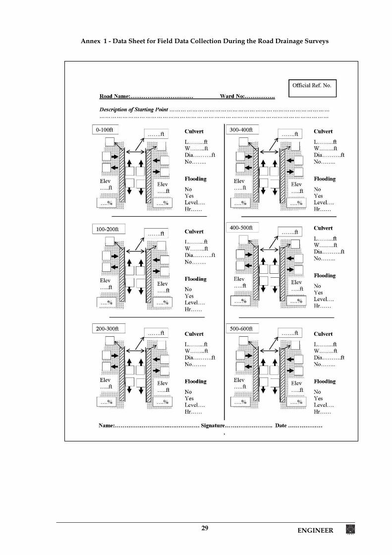
29 ENGINEER

Annex 1 - Data Sheet for Field Data Collection During the Road Drainage Surveys

SECTION II

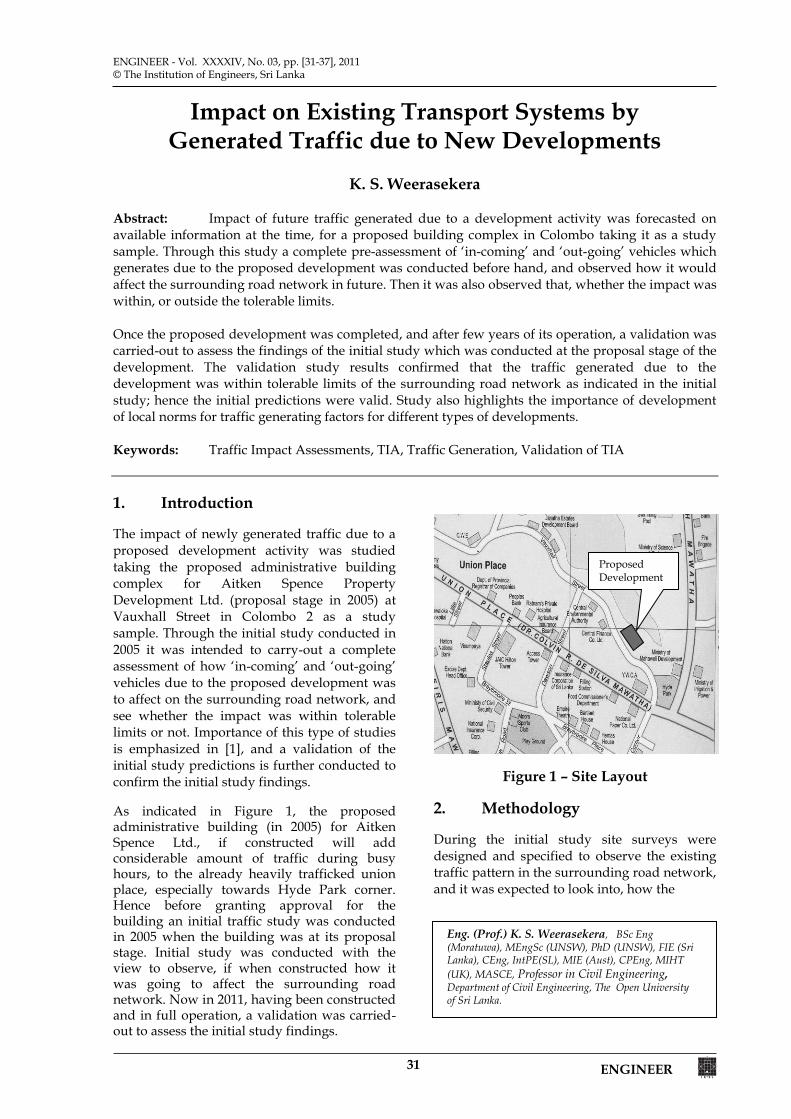
31 ENGINEER

ENGINEER - Vol. XXXXIV, No. 03, pp. [31-37], 2011© The Institution of Engineers, Sri Lanka

Impact on Existing Transport Systems by Generated Traffic due to New Developments

K. S. Weerasekera

Abstract: Impact of future traffic generated due to a development activity was forecasted on available information at the time, for a proposed building complex in Colombo taking it as a study sample. Through this study a complete pre-assessment of ‘in-coming’ and ‘out-going’ vehicles which generates due to the proposed development was conducted before hand, and observed how it would affect the surrounding road network in future. Then it was also observed that, whether the impact was within, or outside the tolerable limits. Once the proposed development was completed, and after few years of its operation, a validation was carried-out to assess the findings of the initial study which was conducted at the proposal stage of the development. The validation study results confirmed that the traffic generated due to the development was within tolerable limits of the surrounding road network as indicated in the initial study; hence the initial predictions were valid. Study also highlights the importance of development of local norms for traffic generating factors for different types of developments. Keywords: Traffic Impact Assessments, TIA, Traffic Generation, Validation of TIA 1. Introduction

The impact of newly generated traffic due to a proposed development activity was studied taking the proposed administrative building complex for Aitken Spence Property Development Ltd. (proposal stage in 2005) at Vauxhall Street in Colombo 2 as a study sample. Through the initial study conducted in 2005 it was intended to carry-out a complete assessment of how ‘in-coming’ and ‘out-going’ vehicles due to the proposed development was to affect on the surrounding road network, and see whether the impact was within tolerable limits or not. Importance of this type of studies is emphasized in [1], and a validation of the initial study predictions is further conducted to confirm the initial study findings.

As indicated in Figure 1, the proposed administrative building (in 2005) for Aitken Spence Ltd., if constructed will add considerable amount of traffic during busy hours, to the already heavily trafficked union place, especially towards Hyde Park corner. Hence before granting approval for the building an initial traffic study was conducted in 2005 when the building was at its proposal stage. Initial study was conducted with the view to observe, if when constructed how it was going to affect the surrounding road network. Now in 2011, having been constructed and in full operation, a validation was carried-out to assess the initial study findings.

Figure 1 – Site Layout

2. Methodology

During the initial study site surveys were designed and specified to observe the existing traffic pattern in the surrounding road network, and it was expected to look into, how the

Proposed Development

Eng. (Prof.) K. S. Weerasekera, BSc Eng (Moratuwa), MEngSc (UNSW), PhD (UNSW), FIE (Sri Lanka), CEng, IntPE(SL), MIE (Aust), CPEng, MIHT (UK), MASCE, Professor in Civil Engineering, Department of Civil Engineering, The Open University of Sri Lanka.

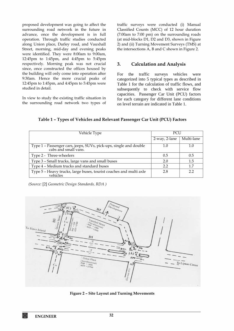
ENGINEER 32

proposed development was going to affect the surrounding road network in the future in advance, once the development is in full operation. Through traffic studies conducted along Union place, Darley road, and Vauxhall Street, morning, mid-day and evening peaks were identified. They were 8:00am to 9:00am, 12:45pm to 1:45pm, and 4:45pm to 5:45pm respectively. Morning peak was not crucial since, once constructed the offices housed by the building will only come into operation after 9:30am. Hence the more crucial peaks of 12:45pm to 1:45pm, and 4:45pm to 5:45pm were studied in detail. In view to study the existing traffic situation in the surrounding road network two types of

traffic surveys were conducted (i) Manual Classified Counts (MCC) of 12 hour duration (7:00am to 7:00 pm) on the surrounding roads (at mid-blocks D1, D2 and D3, shown in Figure 2) and (ii) Turning Movement Surveys (TMS) at the intersections A, B and C shown in Figure 2. 3. Calculation and Analysis For the traffic surveys vehicles were categorized into 5 typical types as described in Table 1 for the calculation of traffic flows, and subsequently to check with service flow capacities. Passenger Car Unit (PCU) factors for each category for different lane conditions on level terrain are indicated in Table 1.

Table 1 – Types of Vehicles and Relevant Passenger Car Unit (PCU) Factors

Vehicle Type PCU

2-way, 2-lane Multi-lane

Type 1 – Passenger cars, jeeps, SUVs, pick-ups, single and double cabs and small vans.

1.0 1.0

Type 2 - Three-wheelers 0.5 0.5 Type 3 – Small trucks, large vans and small buses 2.0 1.5 Type 4 – Medium trucks and standard buses 2.2 1.7 Type 5 – Heavy trucks, large buses, tourist coaches and multi axle

vehicles 2.8 2.2

(Source: [2] Geometric Design Standards, RDA )

Figure 2 – Site Layout and Turning Movements

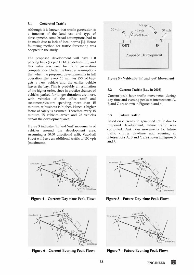
33 ENGINEER

3.1 Generated Traffic

Although it is known that traffic generation is a function of the land use and type of development, some broad assumptions had to be made due to lack of local norms [3]. Hence following method for traffic forecasting was adopted in the study. The proposed development will have 100 parking bays (as per UDA guidelines [5]), and this value was used for traffic generation computations. Under the broader assumptions that when the proposed development is in full operation, that every 15 minutes 25% of bays gets a new vehicle and the earlier vehicle leaves the bay. This is probably an estimation of the higher order, since in practice chances of vehicles parked for longer durations are more, with vehicles of the office staff and customers/visitors spending more than 45 minutes at business is higher. Hence a higher factor of safety is assumed. Therefore every 15 minutes 25 vehicles arrive and 25 vehicles depart the development area.

Figure 3 indicates ‘in’ and ‘out’ movements of vehicles around the development area. Assuming a 50:50 directional split, Vauxhall Street will have an additional traffic of 100 vph (maximum).

Figure 3 – Vehicular ‘in’ and ‘out’ Movement

3.2 Current Traffic (i.e., in 2005)

Current peak hour traffic movements during day-time and evening peaks at intersections A, B and C are shown in Figures 4 and 6.

3.3 Future Traffic

Based on current and generated traffic due to proposed development, future traffic was computed. Peak hour movements for future traffic during day-time and evening at intersections A, B and C are shown in Figures 5 and 7.

Figure 4 – Current Day-time Peak Flows Figure 5 – Future Day-time Peak Flows

Figure 6 – Current Evening Peak Flows Figure 7 – Future Evening Peak Flows

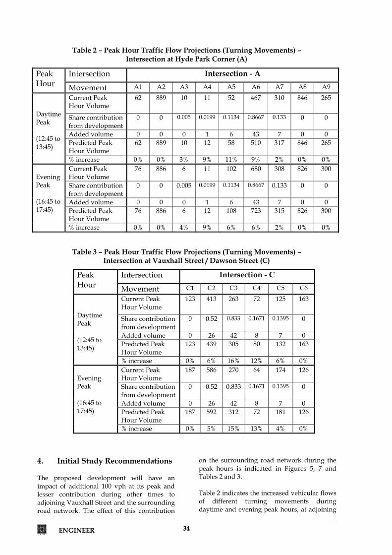
ENGINEER 34

Table 2 – Peak Hour Traffic Flow Projections (Turning Movements) –

Intersection at Hyde Park Corner (A)

Peak Hour

Intersection Intersection - A

Movement A1 A2 A3 A4 A5 A6 A7 A8 A9 Daytime Peak (12:45 to 13:45)

Current Peak Hour Volume

62 889 10 11 52 467 310 846 265

Share contribution from development

0 0 0.005 0.0199 0.1134 0.8667 0.133 0 0

Added volume 0 0 0 1 6 43 7 0 0 Predicted Peak Hour Volume

62 889 10 12 58 510 317 846 265

% increase 0% 0% 3% 9% 11% 9% 2% 0% 0% Evening Peak (16:45 to 17:45)

Current Peak Hour Volume

76 886 6 11 102 680 308 826 300

Share contribution from development

0 0 0.005 0.0199 0.1134 0.8667 0.133 0 0

Added volume 0 0 0 1 6 43 7 0 0 Predicted Peak Hour Volume

76 886 6 12 108 723 315 826 300

% increase 0% 0% 4% 9% 6% 6% 2% 0% 0%

Table 3 – Peak Hour Traffic Flow Projections (Turning Movements) –

Intersection at Vauxhall Street / Dawson Street (C)

Peak Hour

Intersection Intersection - C

Movement C1 C2 C3 C4 C5 C6 Daytime Peak (12:45 to 13:45)

Current Peak Hour Volume

123 413 263 72 125 163

Share contribution from development

0 0.52 0.833 0.1671 0.1395 0

Added volume 0 26 42 8 7 0 Predicted Peak Hour Volume

123 439 305 80 132 163

% increase 0% 6% 16% 12% 6% 0% Evening Peak (16:45 to 17:45)

Current Peak Hour Volume

187 586 270 64 174 126

Share contribution from development

0 0.52 0.833 0.1671 0.1395 0

Added volume 0 26 42 8 7 0 Predicted Peak Hour Volume

187 592 312 72 181 126

% increase 0% 5% 15% 13% 4% 0%

4. Initial Study Recommendations The proposed development will have an impact of additional 100 vph at its peak and lesser contribution during other times to adjoining Vauxhall Street and the surrounding road network. The effect of this contribution

on the surrounding road network during the peak hours is indicated in Figures 5, 7 and Tables 2 and 3. Table 2 indicates the increased vehicular flows of different turning movements during daytime and evening peak hours, at adjoining

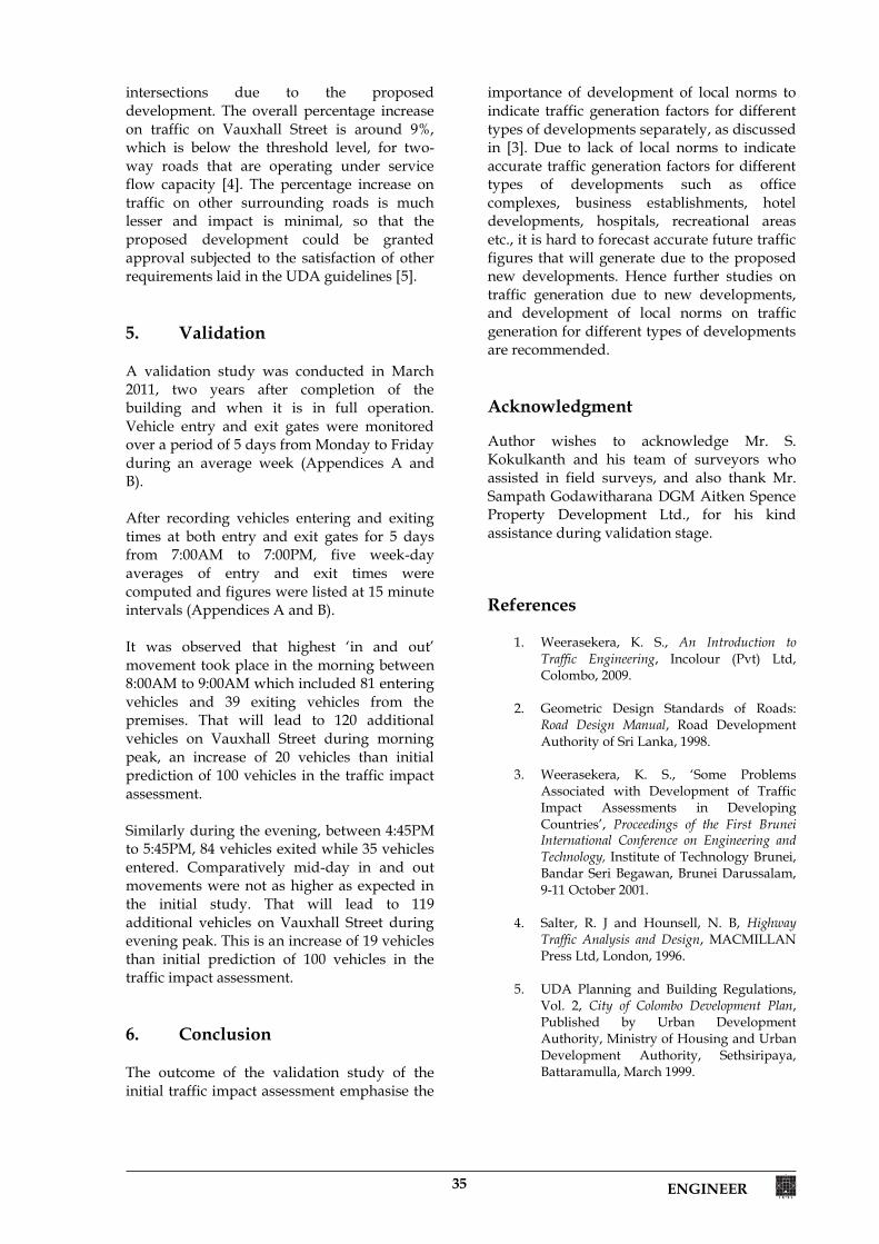
35 ENGINEER

intersections due to the proposed development. The overall percentage increase on traffic on Vauxhall Street is around 9%, which is below the threshold level, for two-way roads that are operating under service flow capacity [4]. The percentage increase on traffic on other surrounding roads is much lesser and impact is minimal, so that the proposed development could be granted approval subjected to the satisfaction of other requirements laid in the UDA guidelines [5]. 5. Validation A validation study was conducted in March 2011, two years after completion of the building and when it is in full operation. Vehicle entry and exit gates were monitored over a period of 5 days from Monday to Friday during an average week (Appendices A and B). After recording vehicles entering and exiting times at both entry and exit gates for 5 days from 7:00AM to 7:00PM, five week-day averages of entry and exit times were computed and figures were listed at 15 minute intervals (Appendices A and B). It was observed that highest ‘in and out’ movement took place in the morning between 8:00AM to 9:00AM which included 81 entering vehicles and 39 exiting vehicles from the premises. That will lead to 120 additional vehicles on Vauxhall Street during morning peak, an increase of 20 vehicles than initial prediction of 100 vehicles in the traffic impact assessment. Similarly during the evening, between 4:45PM to 5:45PM, 84 vehicles exited while 35 vehicles entered. Comparatively mid-day in and out movements were not as higher as expected in the initial study. That will lead to 119 additional vehicles on Vauxhall Street during evening peak. This is an increase of 19 vehicles than initial prediction of 100 vehicles in the traffic impact assessment. 6. Conclusion The outcome of the validation study of the initial traffic impact assessment emphasise the

importance of development of local norms to indicate traffic generation factors for different types of developments separately, as discussed in [3]. Due to lack of local norms to indicate accurate traffic generation factors for different types of developments such as office complexes, business establishments, hotel developments, hospitals, recreational areas etc., it is hard to forecast accurate future traffic figures that will generate due to the proposed new developments. Hence further studies on traffic generation due to new developments, and development of local norms on traffic generation for different types of developments are recommended. Acknowledgment

Author wishes to acknowledge Mr. S. Kokulkanth and his team of surveyors who assisted in field surveys, and also thank Mr. Sampath Godawitharana DGM Aitken Spence Property Development Ltd., for his kind assistance during validation stage.

References

1. Weerasekera, K. S., An Introduction to Traffic Engineering, Incolour (Pvt) Ltd, Colombo, 2009.

2. Geometric Design Standards of Roads:

Road Design Manual, Road Development Authority of Sri Lanka, 1998.

3. Weerasekera, K. S., ‘Some Problems Associated with Development of Traffic Impact Assessments in Developing Countries’, Proceedings of the First Brunei International Conference on Engineering and Technology, Institute of Technology Brunei, Bandar Seri Begawan, Brunei Darussalam, 9-11 October 2001.

4. Salter, R. J and Hounsell, N. B, Highway

Traffic Analysis and Design, MACMILLAN Press Ltd, London, 1996.

5. UDA Planning and Building Regulations,

Vol. 2, City of Colombo Development Plan, Published by Urban Development Authority, Ministry of Housing and Urban Development Authority, Sethsiripaya, Battaramulla, March 1999.

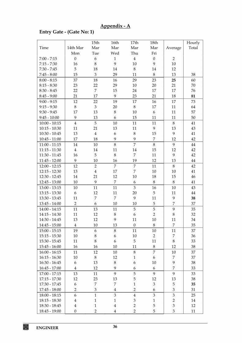
ENGINEER 36

Appendix - AEntry Gate - (Gate No: 1)

Time 14th Mar 15th Mar

16th Mar

17th Mar

18th Mar Average

Hourly Total

Mon Tue Wed Thu Fri 7:00 - 7:15 0 6 1 4 0 2 7:15 - 7:30 16 8 9 10 9 10 7:30 - 7:45 5 18 14 8 14 12 7:45 - 8:00 15 3 29 11 8 13 38 8:00 - 8:15 37 18 16 29 23 25 60 8:15 - 8:30 23 22 29 10 20 21 70 8:30 - 8:45 22 7 15 24 17 17 76 8:45 - 9:00 21 17 9 23 21 18 81 9:00 - 9:15 12 22 19 17 16 17 73 9:15 - 9:30 8 3 20 8 17 11 64 9:30 - 9:45 17 13 8 10 6 11 57 9:45 - 10:00 9 13 6 15 11 11 50 10:00 - 10:15 4 5 10 11 11 8 41 10:15 - 10:30 11 21 13 11 9 13 43 10:30 - 10:45 13 4 6 8 15 9 41 10:45 - 11:00 17 18 9 9 7 12 42 11:00 - 11:15 14 10 8 7 8 9 44 11:15 - 11:30 4 14 11 14 15 12 42 11:30 - 11:45 16 5 8 7 11 9 42 11:45 - 12:00 9 10 16 19 12 13 44 12:00 - 12:15 12 2 7 7 11 8 42 12:15 - 12:30 13 4 17 7 10 10 41 12:30 - 12:45 14 21 12 10 18 15 46 12:45 - 13:00 10 9 7 6 8 8 41 13:00 - 13:15 10 11 11 3 16 10 43 13:15 - 13:30 6 12 11 20 5 11 44 13:30 - 13:45 11 7 7 9 11 9 38 13:45 - 14:00 2 6 10 10 5 7 37 14:00 - 14:15 11 13 11 5 5 9 35 14:15 - 14:30 11 12 8 6 2 8 32 14:30 - 14:45 13 12 9 11 10 11 34 14:45 - 15:00 4 10 13 0 8 7 35 15:00 - 15:15 19 6 8 11 10 11 37 15:15 - 15:30 10 8 6 10 2 7 36 15:30 - 15:45 11 8 6 5 11 8 33 15:45 - 16:00 16 16 10 11 8 12 38 16:00 - 16:15 11 12 10 8 7 10 37 16:15 - 16:30 10 8 12 1 6 7 37 16:30 - 16:45 6 13 8 6 10 9 38 16:45 - 17:00 4 12 9 6 6 7 33 17:00 - 17:15 13 11 9 5 9 9 33 17:15 - 17:30 12 23 13 5 12 13 38 17:30 - 17:45 6 7 7 1 3 5 35 17:45 - 18:00 2 3 4 2 6 3 31 18:00 - 18:15 6 1 3 4 3 3 25 18:15 - 18:30 4 1 1 3 1 2 14 18:30 - 18:45 4 1 4 2 5 3 12 18:45 - 19:00 0 2 4 2 5 3 11

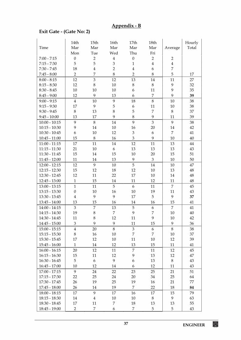
37 ENGINEER

Appendix - B Exit Gate - (Gate No: 2)

Time 14th Mar

15th Mar

16th Mar

17th Mar

18th Mar Average

Hourly Total

Mon Tue Wed Thu Fri 7:00 - 7:15 0 2 4 0 2 2 7:15 - 7:30 5 5 3 1 4 4 7:30 - 7:45 18 4 2 4 6 7 7:45 - 8:00 2 7 8 2 8 5 17 8:00 - 8:15 12 3 12 13 14 11 27 8:15 - 8:30 12 8 10 8 8 9 32 8:30 - 8:45 10 10 10 6 11 9 35 8:45 - 9:00 12 9 13 6 7 9 39 9:00 - 9:15 4 10 9 18 8 10 38 9:15 - 9:30 17 9 5 6 11 10 38 9:30 - 9:45 8 13 8 5 7 8 37 9:45 - 10:00 13 17 9 8 9 11 39 10:00 - 10:15 9 8 14 9 3 9 38 10:15 - 10:30 9 14 10 16 20 14 42 10:30 - 10:45 6 10 12 3 6 7 41 10:45 - 11:00 15 8 16 3 9 10 40 11:00 - 11:15 17 11 14 12 11 13 44 11:15 - 11:30 21 10 6 13 13 13 43 11:30 - 11:45 15 14 15 10 20 15 51 11:45 - 12:00 11 14 13 9 3 10 50 12:00 - 12:15 12 9 10 5 14 10 47 12:15 - 12:30 15 12 18 12 10 13 48 12:30 - 12:45 12 11 22 17 10 14 48 12:45 - 13:00 1 15 14 11 12 11 48 13:00 - 13:15 1 11 5 6 11 7 45 13:15 - 13:30 0 10 16 10 19 11 43 13:30 - 13:45 4 9 9 17 5 9 37 13:45 - 14:00 13 15 16 14 16 15 41 14:00 - 14:15 3 7 13 5 6 7 41 14:15 - 14:30 19 8 7 9 7 10 40 14:30 - 14:45 11 8 12 11 9 10 42 14:45 - 15:00 3 9 9 11 15 9 36 15:00 - 15:15 4 20 8 3 6 8 38 15:15 - 15:30 8 16 10 7 7 10 37 15:30 - 15:45 17 12 10 11 10 12 39 15:45 - 16:00 1 14 12 13 15 11 41 16:00 - 16:15 20 12 11 7 11 12 45 16:15 - 16:30 15 11 12 9 13 12 47 16:30 - 16:45 5 6 9 6 13 8 43 16:45 - 17:00 10 12 14 6 12 11 43 17:00 - 17:15 9 24 22 23 25 21 51 17:15 - 17:30 22 25 24 20 34 25 64 17:30 - 17:45 26 19 25 19 16 21 77 17:45 - 18:00 26 14 19 7 22 18 84 18:00 - 18:15 17 9 17 16 17 15 79 18:15 - 18:30 14 4 10 10 8 9 63 18:30 - 18:45 17 11 7 18 13 13 55 18:45 - 19:00 2 7 6 7 5 5 43

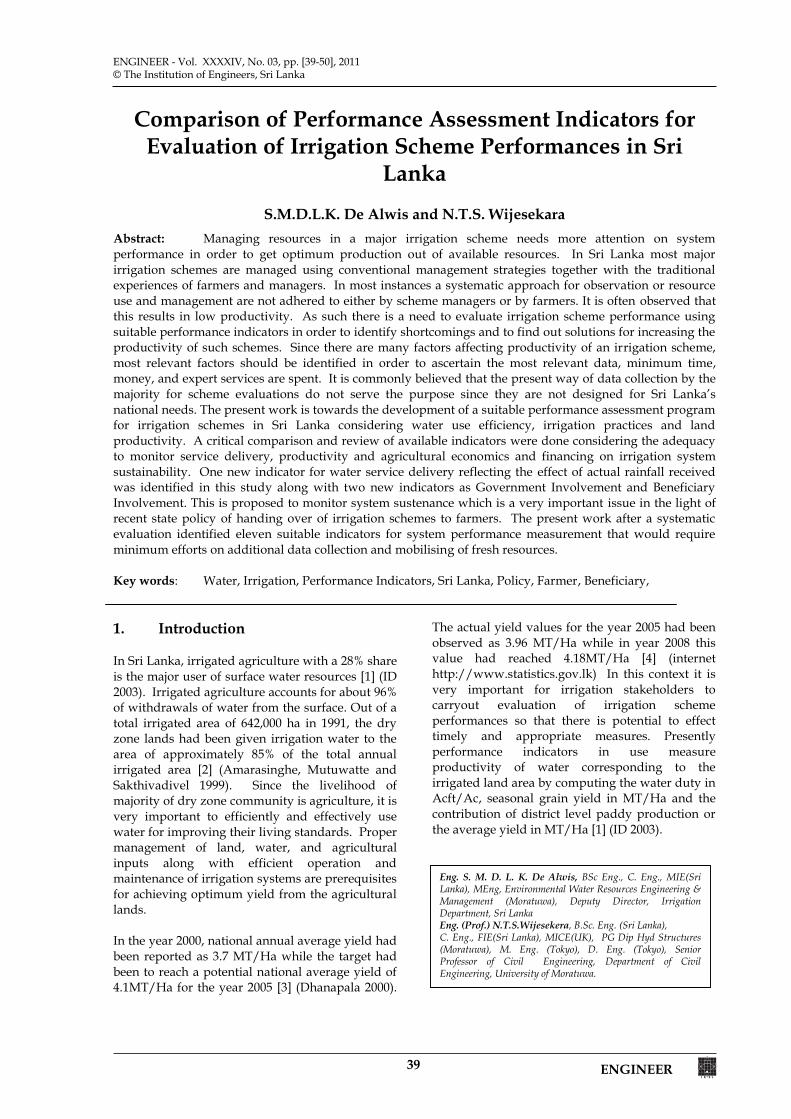
39 ENGINEER

ENGINEER - Vol. XXXXIV, No. 03, pp. [39-50], 2011© The Institution of Engineers, Sri Lanka

Comparison of Performance Assessment Indicators for Evaluation of Irrigation Scheme Performances in Sri

Lanka

S.M.D.L.K. De Alwis and N.T.S. Wijesekara

Abstract: Managing resources in a major irrigation scheme needs more attention on system performance in order to get optimum production out of available resources. In Sri Lanka most major irrigation schemes are managed using conventional management strategies together with the traditional experiences of farmers and managers. In most instances a systematic approach for observation or resource use and management are not adhered to either by scheme managers or by farmers. It is often observed that this results in low productivity. As such there is a need to evaluate irrigation scheme performance using suitable performance indicators in order to identify shortcomings and to find out solutions for increasing the productivity of such schemes. Since there are many factors affecting productivity of an irrigation scheme, most relevant factors should be identified in order to ascertain the most relevant data, minimum time, money, and expert services are spent. It is commonly believed that the present way of data collection by the majority for scheme evaluations do not serve the purpose since they are not designed for Sri Lanka’s national needs. The present work is towards the development of a suitable performance assessment program for irrigation schemes in Sri Lanka considering water use efficiency, irrigation practices and land productivity. A critical comparison and review of available indicators were done considering the adequacy to monitor service delivery, productivity and agricultural economics and financing on irrigation system sustainability. One new indicator for water service delivery reflecting the effect of actual rainfall received was identified in this study along with two new indicators as Government Involvement and Beneficiary Involvement. This is proposed to monitor system sustenance which is a very important issue in the light of recent state policy of handing over of irrigation schemes to farmers. The present work after a systematic evaluation identified eleven suitable indicators for system performance measurement that would require minimum efforts on additional data collection and mobilising of fresh resources. Key words: Water, Irrigation, Performance Indicators, Sri Lanka, Policy, Farmer, Beneficiary, 1. Introduction In Sri Lanka, irrigated agriculture with a 28% share is the major user of surface water resources [1] (ID 2003). Irrigated agriculture accounts for about 96% of withdrawals of water from the surface. Out of a total irrigated area of 642,000 ha in 1991, the dry zone lands had been given irrigation water to the area of approximately 85% of the total annual irrigated area [2] (Amarasinghe, Mutuwatte and Sakthivadivel 1999). Since the livelihood of majority of dry zone community is agriculture, it is very important to efficiently and effectively use water for improving their living standards. Proper management of land, water, and agricultural inputs along with efficient operation and maintenance of irrigation systems are prerequisites for achieving optimum yield from the agricultural lands. In the year 2000, national annual average yield had been reported as 3.7 MT/Ha while the target had been to reach a potential national average yield of 4.1MT/Ha for the year 2005 [3] (Dhanapala 2000).

The actual yield values for the year 2005 had been observed as 3.96 MT/Ha while in year 2008 this value had reached 4.18MT/Ha [4] (internet http://www.statistics.gov.lk) In this context it is very important for irrigation stakeholders to carryout evaluation of irrigation scheme performances so that there is potential to effect timely and appropriate measures. Presently performance indicators in use measure productivity of water corresponding to the irrigated land area by computing the water duty in Acft/Ac, seasonal grain yield in MT/Ha and the contribution of district level paddy production or the average yield in MT/Ha [1] (ID 2003).

Eng. S. M. D. L. K. De Alwis, BSc Eng., C. Eng., MIE(Sri Lanka), MEng, Environmental Water Resources Engineering & Management (Moratuwa), Deputy Director, Irrigation Department, Sri Lanka Eng. (Prof.) N.T.S.Wijesekera, B.Sc. Eng. (Sri Lanka), C. Eng., FIE(Sri Lanka), MICE(UK), PG Dip Hyd Structures (Moratuwa), M. Eng. (Tokyo), D. Eng. (Tokyo), Senior Professor of Civil Engineering, Department of Civil Engineering, University of Moratuwa.

ENGINEER 40

It has been noted that water duty values at the end of the season provide the overall water

consumption of the area, do not provide

adequate information about the adequacy, reliability and timeliness of operations. Average yield which provides average productivity per unit area does not reflect the reasons for such yields. Literature indicated that most agriculture production indicators enable assessment of the performance of a season in terms of a selected criterion with respect to benchmark values. However scheme level benchmark values were not available at the Department of Agriculture except district level yield forecasts. In order to assess the Agriculture Economics & Financing, status of the irrigated agriculture sector, the most common indicator used in Sri Lanka is ‘Profit’ which usually presents the national level performance using district level values [5] DOA(2005). There are a large number of indicators presented in the literature together with those already in use enabling an irrigation manager to identify the effectiveness and efficiency of land and water resource usage ([1] ID 2003, [6] Bos Burton and Molden 2005, [7] Malano and Burton 2001). [8] Murray-Rust and Snellen (1993) carrying out an irrigation system case study including four schemes from Sri Lanka has indicated that lack of systematic measurement of performance, minimum concern about long term sustainability and poor consideration of institutional and resource condition are key factors that need to be addressed in the performance assessment of irrigated agriculture. [6] BOS, Burton, and Molden (2005) in their guideline very clearly indicate that the assessment of performance assessment procedure would vary depending on the purpose of the assessment and the type of scheme. In almost all irrigation schemes there are several indicators computed resulting from a vast data collection effort. However there are no supporting literatures or case studies to guide a scheme manager about the best indicators that could be used with either already collected data or with a minimum additional data collection effort. Therefore it is very important to carefully evaluate these indicators for the identification of the optimum effective management of the spatial units starting from irrigation scheme as operational units.

Informal discussions had with irrigation managers and farmers revealed that some of the important questions that require answers are the identification of operational performance of irrigation scheme tracts, productivity of turnout areas, performance of irrigation practices and assessment of profitability. Accordingly it is necessary to identify information

pertaining to three major categories as (i) service delivery, (ii) production (iii) economics & financing.

In this backdrop, the objective of the present work is to carryout a comparison of most common irrigation performance indicators to identify the best for Sri Lanka in order to address water use efficiency, irrigation practices, land productivity and system sustenance etc., with respect to water, yield and income consideration of Irrigation Department and the Farmer Organisations who are the two major stakeholder groups in the irrigation sector.

In the present work extensive discussions were held with irrigation managers and farmer organisation representatives to capture performance assessment needs especially in a turnout area basis for productivity enhancement. They are water utilisation and service delivery, land utilization, effective use of rainfall for production, provision of engineering and agricultural inputs, government support, and strength of farmer organizations and the enhancement of farmer status. The literature survey for the present work identified eleven major documents describing and discussing performance indicators that are relevant to the study objectives and number of indicators were captured with a listing of an associated categorisation (Table 1).

2.0 Methodology and Analysis 2.1 Literature Survey Performance assessment is the systematic observation, documentation and interpretation of the management of an irrigation and drainage system to ensure intended outputs and proper functioning ([6] Bos, Burton and Molden 2005). The three key stakeholder interactions that have been identified in the irrigated agricultural sector are between, i) Water Institutions and Farmer Organizations, ii) Farmer Organizations and the Government and iii) Water Institutions and the Government ([9] Bandara 2006). Performance optimization of irrigation schemes is commonly applied either through planning, management, or structural interventions to improve application, conveyance or economic efficiency ([10] Jayatillake 2000).

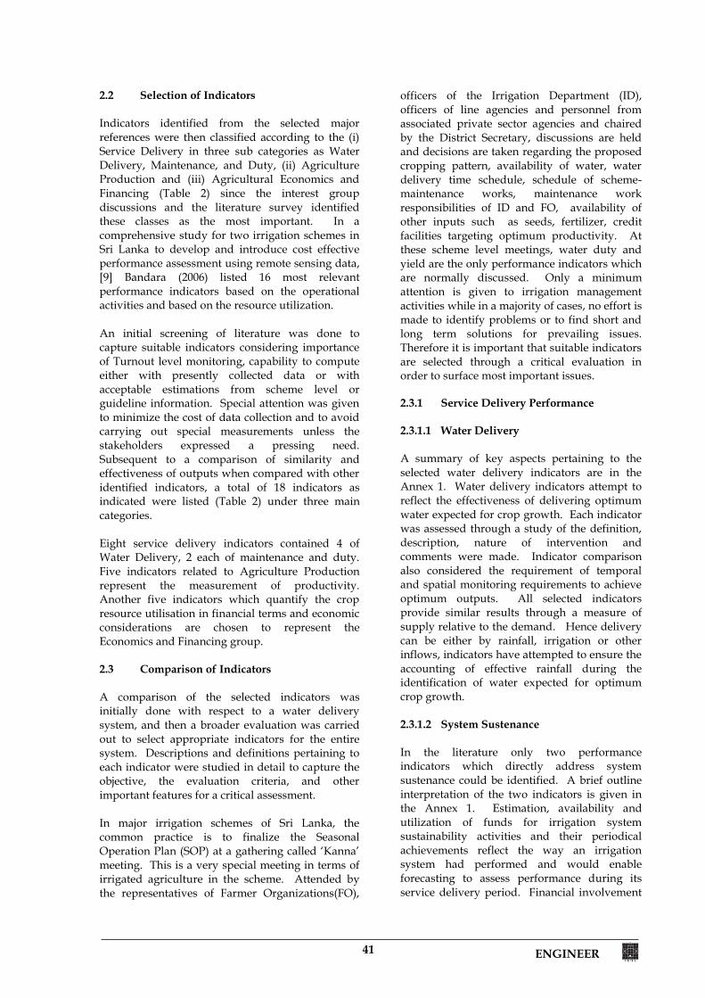
41 ENGINEER

2.2 Selection of Indicators Indicators identified from the selected major references were then classified according to the (i) Service Delivery in three sub categories as Water Delivery, Maintenance, and Duty, (ii) Agriculture Production and (iii) Agricultural Economics and Financing (Table 2) since the interest group discussions and the literature survey identified these classes as the most important. In a comprehensive study for two irrigation schemes in Sri Lanka to develop and introduce cost effective performance assessment using remote sensing data, [9] Bandara (2006) listed 16 most relevant performance indicators based on the operational activities and based on the resource utilization. An initial screening of literature was done to capture suitable indicators considering importance of Turnout level monitoring, capability to compute either with presently collected data or with acceptable estimations from scheme level or guideline information. Special attention was given to minimize the cost of data collection and to avoid carrying out special measurements unless the stakeholders expressed a pressing need. Subsequent to a comparison of similarity and effectiveness of outputs when compared with other identified indicators, a total of 18 indicators as indicated were listed (Table 2) under three main categories. Eight service delivery indicators contained 4 of Water Delivery, 2 each of maintenance and duty. Five indicators related to Agriculture Production represent the measurement of productivity. Another five indicators which quantify the crop resource utilisation in financial terms and economic considerations are chosen to represent the Economics and Financing group. 2.3 Comparison of Indicators A comparison of the selected indicators was initially done with respect to a water delivery system, and then a broader evaluation was carried out to select appropriate indicators for the entire system. Descriptions and definitions pertaining to each indicator were studied in detail to capture the objective, the evaluation criteria, and other important features for a critical assessment. In major irrigation schemes of Sri Lanka, the common practice is to finalize the Seasonal Operation Plan (SOP) at a gathering called ‘Kanna’ meeting. This is a very special meeting in terms of irrigated agriculture in the scheme. Attended by the representatives of Farmer Organizations(FO),

officers of the Irrigation Department (ID), officers of line agencies and personnel from associated private sector agencies and chaired by the District Secretary, discussions are held and decisions are taken regarding the proposed cropping pattern, availability of water, water delivery time schedule, schedule of scheme-maintenance works, maintenance work responsibilities of ID and FO, availability of other inputs such as seeds, fertilizer, credit facilities targeting optimum productivity. At these scheme level meetings, water duty and yield are the only performance indicators which are normally discussed. Only a minimum attention is given to irrigation management activities while in a majority of cases, no effort is made to identify problems or to find short and long term solutions for prevailing issues. Therefore it is important that suitable indicators are selected through a critical evaluation in order to surface most important issues. 2.3.1 Service Delivery Performance 2.3.1.1 Water Delivery A summary of key aspects pertaining to the selected water delivery indicators are in the Annex 1. Water delivery indicators attempt to reflect the effectiveness of delivering optimum water expected for crop growth. Each indicator was assessed through a study of the definition, description, nature of intervention and comments were made. Indicator comparison also considered the requirement of temporal and spatial monitoring requirements to achieve optimum outputs. All selected indicators provide similar results through a measure of supply relative to the demand. Hence delivery can be either by rainfall, irrigation or other inflows, indicators have attempted to ensure the accounting of effective rainfall during the identification of water expected for optimum crop growth. 2.3.1.2 System Sustenance In the literature only two performance indicators which directly address system sustenance could be identified. A brief outline interpretation of the two indicators is given in the Annex 1. Estimation, availability and utilization of funds for irrigation system sustainability activities and their periodical achievements reflect the way an irrigation system had performed and would enable forecasting to assess performance during its service delivery period. Financial involvement

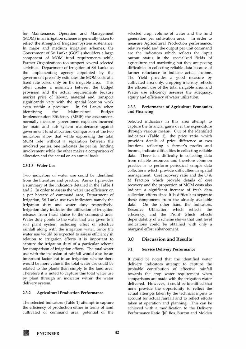
ENGINEER 42

for Maintenance, Operation and Management (MOM) in an irrigation scheme is generally taken to reflect the strength of Irrigation System sustenance. In major and medium irrigation schemes, the Government of Sri Lanka (GOSL) shoulders a large component of MOM fund requirements while Farmer Organizations too support several selected activities. Department of Irrigation of Sri Lanka as the implementing agency appointed by the government presently estimates the MOM costs at a fixed rate based only on the irrigable area. This often creates a mismatch between the budget provision and the actual requirements because market price of labour, material and transport significantly vary with the spatial location work even within a province. In Sri Lanka when identifying the Maintenance Budget Implementation Efficiency (MBIE) the assessments normally measure government expenses incurred for main and sub system maintenance against government fund allocation. Comparison of the two indicators show that while expressing the total MOM role without a separation between the involved parties, one indicates the per ha funding involvement while the other makes a comparison of allocation and the actual on an annual basis. 2.3.1.3 Water Use Two indicators of water use could be identified from the literature and practice. Annex 1 provides a summary of the indicators detailed in the Table 1 and 2. In order to assess the water use efficiency on a per hectare of command area, Department of Irrigation, Sri Lanka use two indicators namely the irrigation duty and water duty respectively. Irrigation duty indicates the utilization of irrigation releases from head sluice to the command area. Water duty points to the water that was given to a soil plant system including effect of effective rainfall along with the irrigation water. Since the water use would be expected to assess efficiency in relation to irrigation efforts it is important to capture the irrigation duty of a particular scheme for comparison of irrigation efforts. The total water use with the inclusion of rainfall would also be an important factor but in an irrigation scheme there would be more value if the total water use could be related to the plants than simply to the land area. Therefore it is noted to capture this total water use by plant through an indicator within the water delivery system.

2.3.2 Agricultural Production Performance The selected indicators (Table 1) attempt to capture the efficiency of production either in terms of land cultivated or command area, potential of the

selected crop, volume of water and the fund generation per cultivation area. In order to measure Agricultural Production performance, relative yield and the output per unit command are the indicators which reflects the input output status in the specialized fields of agriculture and marketing but they are posing difficulties in collecting reliable data because of farmer reluctance to indicate actual income. The Yield provides a good measure by cultivated area only, cropping intensity reflects the efficient use of the total irrigable area, and Water use efficiency assesses the adequacy, equity and efficiency of water utilization. 2.3.3 Performance of Agriculture Economics and Financing Selected indicators in this area attempt to capture the financial gains over the expenditure through various means. Out of the identified indicators (Table 1), the price ratio which provides details of price difference at two locations reflecting a farmer’s profits and income, indicate difficulties in collecting reliable data. There is a difficulty in collecting data from reliable resources and therefore common practice is to perform periodical sample data collections which provide difficulties in spatial management. Cost recovery ratio and the O & M Fraction which provide details of cost recovery and the proportion of MOM costs also indicate a significant increase of fresh data collection efforts since it is difficult to separate these components from the already available data. On the other hand the indicators, Resource Utilization which reflects the efficiency, and the Profit which reflects dependability of a scheme shows that unit level indications could be obtained with only a marginal effort enhancement. 3.0 Discussion and Results 3.1 Service Delivery Performance It could be noted that the identified water delivery indicators attempt to capture the probable contribution of effective rainfall towards the crop water requirement when comparisons are made with the irrigation water delivered. However, it could be identified that none provide the opportunity to reflect the actual attempts taken by the technical inputs to account for actual rainfall and to reflect efforts taken at operation and planning. This can be achieved with a modification to the Delivery Performance Ratio ([6] Bos, Burton and Molden

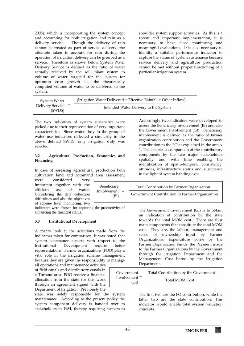
43 ENGINEER

2005), which is incorporating the system concept and accounting for both irrigation and rain as a delivery service. Though the delivery of rain cannot be treated as part of service delivery, the attempts taken to account for rain during the operation of irrigation delivery can be grouped as a service. Therefore as shown below System Water Delivery Service is defined as the ratio of water actually received by the soil, plant system to volume of water targeted for the system for optimum crop growth i.e. the theoretically computed volume of water to be delivered to the system.

The two indicators of system sustenance were picked due to their representation of very important characteristics. Since water duty in the group of water use indicators reflected a similarity in the above defined SWDS, only irrigation duty was selected. 3.2 Agricultural Production, Economics and Financing In case of assessing agricultural production both cultivation land and command area assessment were considered very important together with the efficient use of water. Considering the data collection difficulties and also the objectives of scheme level monitoring, two indicators were chosen for capturing the productivity of enhancing the financial status.

3.3 Institutional Development A macro look at the selections made from the indicators taken for comparison, it was noted that system sustenance aspects with respect to the Institutional Development require better representations. Farmer organizations (FOO) play a vital role in the irrigation scheme management because they are given the responsibility to manage all operations and maintenance activities of field canals and distributory canals in a Turnout area. FOO receive a financial allocation from the state for this work through an agreement signed with the Department of Irrigation. Previously the state was solely responsible for the system maintenance. According to the present policy the system component delivery is handed over to stakeholders in 1984, thereby requiring farmers to

shoulder system support activities. As this is a recent and important implementation, it is necessary to have close monitoring and meaningful evaluations. It is also necessary to identify a suitable performance indicator to capture the status of system sustenance because service delivery and agriculture production cannot be met without proper functioning of a particular irrigation system.

Accordingly two indicators were developed to assess the Beneficiary Involvement (BI) and also the Government Involvement (GI). Beneficiary involvement is defined as the ratio of farmer organization contribution and the Government contribution to the FO as explained in the annex 1. This enables a comparison of the contributory components by the two major stakeholders spatially and with time enabling the identification of spatio-temporal consistency, attitudes, infrastructure status and sustenance in the light of system handing over.

The Government Involvement (GI) is to obtain an indication of contribution by the state towards the total MOM cost. There are four main components that constitute the total MOM cost. They are, the labour, management and sense of ownership input by Farmer Organizations, Expenditure borne by the Farmer Organization Funds, the Payment made to the Farmer Organizations by the Government through the irrigation Department and the Management Cost borne by the Irrigation Department.

The first two are the FO contribution, while the latter two are the state contribution. This indicator would enable total system valuation concepts.

Total Contribution by the Government

Total MOM Cost =

Government Involvement

(GI)

Total Contribution by Farmer Organisation

Government Contribution to Farmer Organization = Beneficiary

Involvement (BI)

(Irrigation Water Delivered + Effective Rainfall + Other Inflow)

Intended Water Delivery to the System = System Water

Delivery Service (SWDS)

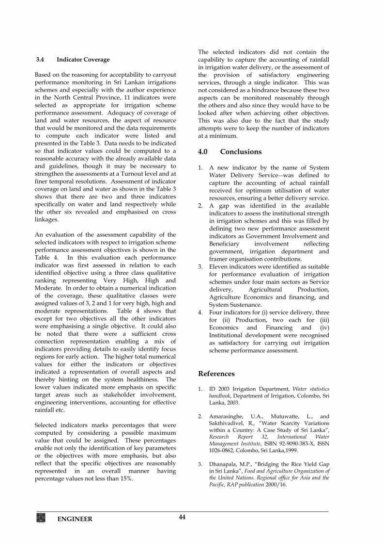
ENGINEER 44

3.4 Indicator Coverage Based on the reasoning for acceptability to carryout performance monitoring in Sri Lankan irrigations schemes and especially with the author experience in the North Central Province, 11 indicators were selected as appropriate for irrigation scheme performance assessment. Adequacy of coverage of land and water resources, the aspect of resource that would be monitored and the data requirements to compute each indicator were listed and presented in the Table 3. Data needs to be indicated so that indicator values could be computed to a reasonable accuracy with the already available data and guidelines, though it may be necessary to strengthen the assessments at a Turnout level and at finer temporal resolutions. Assessment of indicator coverage on land and water as shown in the Table 3 shows that there are two and three indicators specifically on water and land respectively while the other six revealed and emphasised on cross linkages. An evaluation of the assessment capability of the selected indicators with respect to irrigation scheme performance assessment objectives is shown in the Table 4. In this evaluation each performance indicator was first assessed in relation to each identified objective using a three class qualitative ranking representing Very High, High and Moderate. In order to obtain a numerical indication of the coverage, these qualitative classes were assigned values of 3, 2 and 1 for very high, high and moderate representations. Table 4 shows that except for two objectives all the other indicators were emphasising a single objective. It could also be noted that there were a sufficient cross connection representation enabling a mix of indicators providing details to easily identify focus regions for early action. The higher total numerical values for either the indicators or objectives indicated a representation of overall aspects and thereby hinting on the system healthiness. The lower values indicated more emphasis on specific target areas such as stakeholder involvement, engineering interventions, accounting for effective rainfall etc. Selected indicators marks percentages that were computed by considering a possible maximum value that could be assigned. These percentages enable not only the identification of key parameters or the objectives with more emphasis, but also reflect that the specific objectives are reasonably represented in an overall manner having percentage values not less than 15%.

The selected indicators did not contain the capability to capture the accounting of rainfall in irrigation water delivery, or the assessment of the provision of satisfactory engineering services, through a single indicator. This was not considered as a hindrance because these two aspects can be monitored reasonably through the others and also since they would have to be looked after when achieving other objectives. This was also due to the fact that the study attempts were to keep the number of indicators at a minimum. 4.0 Conclusions 1. A new indicator by the name of System

Water Delivery Service was defined to capture the accounting of actual rainfall received for optimum utilisation of water resources, ensuring a better delivery service.

2. A gap was identified in the available indicators to assess the institutional strength in irrigation schemes and this was filled by defining two new performance assessment indicators as Government Involvement and Beneficiary involvement reflecting government, irrigation department and framer organisation contributions.

3. Eleven indicators were identified as suitable for performance evaluation of irrigation schemes under four main sectors as Service delivery, Agricultural Production, Agriculture Economics and financing, and System Sustenance.

4. Four indicators for (i) service delivery, three for (ii) Production, two each for (iii) Economics and Financing and (iv) Institutional development were recognised as satisfactory for carrying out irrigation scheme performance assessment.

References 1. ID 2003 Irrigation Department, Water statistics

handbook, Department of Irrigation, Colombo, Sri Lanka, 2003.

2. Amarasinghe, U.A., Mutuwatte, L., and

Sakthivadivel, R., “Water Scarcity Variations within a Country: A Case Study of Sri Lanka”, Research Report 32, International Water Management Institute, ISBN 92-9090-383-X, ISSN 1026-0862, Colombo, Sri Lanka,1999.

3. Dhanapala, M.P., “Bridging the Rice Yield Gap

in Sri Lanka”, Food and Agriculture Organization of the United Nations. Regional office for Asia and the Pacific, RAP publication 2000/16.

45 ENGINEER

4. Agriculture Statistics of Sri Lanka, Average Yield of

2008, http://www.statistic.gov.lk/agriculture, visited 16th January 2011.

5. DOA (2005), “Cost of Cultivation of Agricultural

Crops Maha 2004/2005”, Publications of Socio Economics and Planning Centre (www.agridept.gov.lk), Department of Agriculture, Peradeniya, Sri Lanka.

6. BOS, M.G., Burton, M.A., Molden, D.J., “Irrigation

and Drainage Performance Assessment”, practical guide line. (ICTAD, CID, IWMT). Ch 3, 2005, pp. 26 – 86 and pp. 144 – 151.

7. Malano, H., and Burton, M., “Guideline for Bench

Marking Performance in the Irrigation and Drainage Sector”, 2001.

8. Murray-Rust, D.H. and Snellen, W.B., “Irrigation

System Performance Assessment and Diagnosis”. Joint IIMI/ILRI/IHEE publication. International Irrigation Management Institute, Colombo, Sri Lanka,1993.

9. Bandara, K.M.P.S., “Assessing Irrigation

Performance by Using Remote Sensing”. ch 3, pp. 27 – 41, ch 7, 2006, pp. 109 – 122.

10. Jayathilake, H.M., “Rice in Major Irrigation Schemes

Potential for Increased Cropping Intensities with Limiting Water Resources: Working paper Rice Congress”. Audio Visual center of the Department of Agriculture, Peradeniya, Sri Lanka. ch 2, 2000, pp. 14 – 63.

11. Bos, M.G. and Nugteren, J., On Irrigation Efficiencies,

2nd edn. ILRI publication No. 19. International Institute for Land Reclamation and Improvement (ILRI), Wageningen, The Netherlands,1974.

12. Molden, D.J., Sakthivadivel, R., Perry, C.J., de

Fraiture, C. and Kloezen, W., “Indicators for Comparing Performance of Irrigated Agricultural Systems”. Research Report 20. International Water Management Institute, Colombo, Sri Lanka,1999.

13. Rao, P.S., “Review of Selected Literature on

Indicators of Irrigation Performance”. IIMI Research paper. International Irrigation Management Institute, Colombo, Sri Lanka. ch 2, pp. 5 -10, ch 3, pp. 55 – 62 and ch 4, 1993, pp. 63 – 64.

14. Diskin Patrick, “Agriculture Productivity Indicator

Measurement Guide”. Food and Nutrition Technical Assistance, 1997, pp 01 – 41.

15. Wim, H., Klozenand & Carlas Garces – Restrepo,

“Assessing Irrigation Performance with comparative Indicators; The Case of Alto Rio Lerma Irrigation District, Mexico”, Research Report 22 IWMI, 1998.

16. Karaa, K., Karam, F., Tarabey. N., “Attempt to

Determine some Performance Indicators in the

QASMEH RAS – EL – AIN Irrigation scheme (Lebanon)”, Technical Paper on Irrigation System Performance.

17. Ponrajah, A.J.P., Revised Edition, “Technical

Guide Line for Irrigation Works, Irrigation Department, Sri Lanka”. 1998, pp. 236 – 249.

18. Siriwardane, S.M.P., “Operational Performance

Monitoring in System C of the Mahaweli Development Programme in Sri Lanka”, 2001.

19. Ariyarathna, D.M., “Towards a New Agriculture

Volume II Ministry of Agriculture and Land, Sri Lanka”,1998.

20. Molden, D., “Accounting for Water Use and

Productivity”. SWIM paper I, International Irrigation Management Institute, Colombo, Sri Lanka,1997.

21. Strzepek, K., Molden, D., Galbraith, H.,

“Comprehensive Globle Assessment of Costs, Benefits and Future Directions of Irrigated Agriculture”, 2001, Working paper 03.

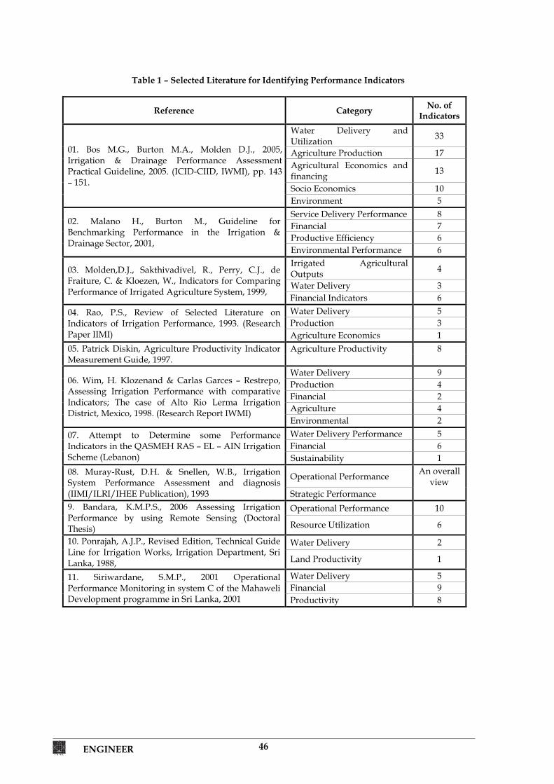
ENGINEER 46

Table 1 – Selected Literature for Identifying Performance Indicators

Reference Category No. of Indicators

01. Bos M.G., Burton M.A., Molden D.J., 2005, Irrigation & Drainage Performance Assessment Practical Guideline, 2005. (ICID-CIID, IWMI), pp. 143 – 151.

Water Delivery and Utilization 33

Agriculture Production 17 Agricultural Economics and financing 13

Socio Economics 10 Environment 5

02. Malano H., Burton M., Guideline for Benchmarking Performance in the Irrigation & Drainage Sector, 2001,

Service Delivery Performance 8 Financial 7 Productive Efficiency 6 Environmental Performance 6

03. Molden,D.J., Sakthivadivel, R., Perry, C.J., de Fraiture, C. & Kloezen, W., Indicators for Comparing Performance of Irrigated Agriculture System, 1999,

Irrigated Agricultural Outputs 4

Water Delivery 3 Financial Indicators 6

04. Rao, P.S., Review of Selected Literature on Indicators of Irrigation Performance, 1993. (Research Paper IIMI)

Water Delivery 5 Production 3 Agriculture Economics 1

05. Patrick Diskin, Agriculture Productivity Indicator Measurement Guide, 1997.

Agriculture Productivity 8

06. Wim, H. Klozenand & Carlas Garces – Restrepo, Assessing Irrigation Performance with comparative Indicators; The case of Alto Rio Lerma Irrigation District, Mexico, 1998. (Research Report IWMI)

Water Delivery 9 Production 4 Financial 2 Agriculture 4 Environmental 2

07. Attempt to Determine some Performance Indicators in the QASMEH RAS – EL – AIN Irrigation Scheme (Lebanon)

Water Delivery Performance 5 Financial 6 Sustainability 1

08. Muray-Rust, D.H. & Snellen, W.B., Irrigation System Performance Assessment and diagnosis (IIMI/ILRI/IHEE Publication), 1993

Operational Performance An overall view

Strategic Performance 9. Bandara, K.M.P.S., 2006 Assessing Irrigation Performance by using Remote Sensing (Doctoral Thesis)

Operational Performance 10

Resource Utilization 6

10. Ponrajah, A.J.P., Revised Edition, Technical Guide Line for Irrigation Works, Irrigation Department, Sri Lanka, 1988,

Water Delivery 2

Land Productivity 1

11. Siriwardane, S.M.P., 2001 Operational Performance Monitoring in system C of the Mahaweli Development programme in Sri Lanka, 2001

Water Delivery 5 Financial 9 Productivity 8

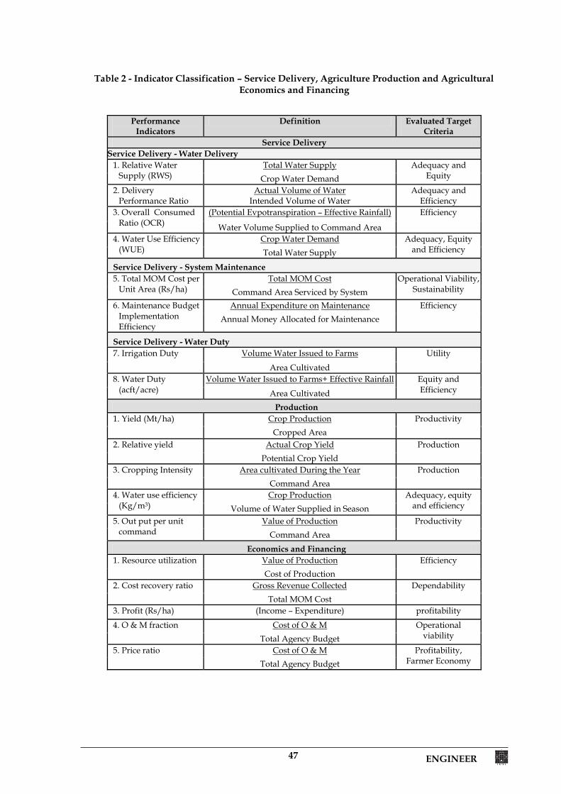
47 ENGINEER

Table 2 - Indicator Classification – Service Delivery, Agriculture Production and Agricultural Economics and Financing

Performance Indicators

Definition Evaluated Target Criteria

Service Delivery Service Delivery - Water Delivery

1. Relative Water Supply (RWS)

Total Water Supply Adequacy and Equity Crop Water Demand

2. Delivery Performance Ratio

Actual Volume of Water Intended Volume of Water

Adequacy and Efficiency

3. Overall Consumed Ratio (OCR)

(Potential Evpotranspiration – Effective Rainfall) Efficiency

Water Volume Supplied to Command Area 4. Water Use Efficiency

(WUE) Crop Water Demand Adequacy, Equity

and Efficiency Total Water Supply

Service Delivery - System Maintenance 5. Total MOM Cost per

Unit Area (Rs/ha) Total MOM Cost Operational Viability,

Sustainability Command Area Serviced by System 6. Maintenance Budget

Implementation Efficiency

Annual Expenditure on Maintenance Efficiency Annual Money Allocated for Maintenance

Service Delivery - Water Duty 7. Irrigation Duty Volume Water Issued to Farms Utility

Area Cultivated 8. Water Duty

(acft/acre) Volume Water Issued to Farms+ Effective Rainfall Equity and

Efficiency Area Cultivated Production

1. Yield (Mt/ha) Crop Production Productivity Cropped Area

2. Relative yield Actual Crop Yield Production Potential Crop Yield

3. Cropping Intensity Area cultivated During the Year Production Command Area

4. Water use efficiency (Kg/m3)

Crop Production Adequacy, equity and efficiency Volume of Water Supplied in Season

5. Out put per unit command

Value of Production Productivity Command Area

Economics and Financing 1. Resource utilization Value of Production Efficiency

Cost of Production 2. Cost recovery ratio Gross Revenue Collected Dependability

Total MOM Cost 3. Profit (Rs/ha) (Income – Expenditure) profitability

4. O & M fraction Cost of O & M Operational viability Total Agency Budget

5. Price ratio Cost of O & M Profitability, Farmer Economy Total Agency Budget

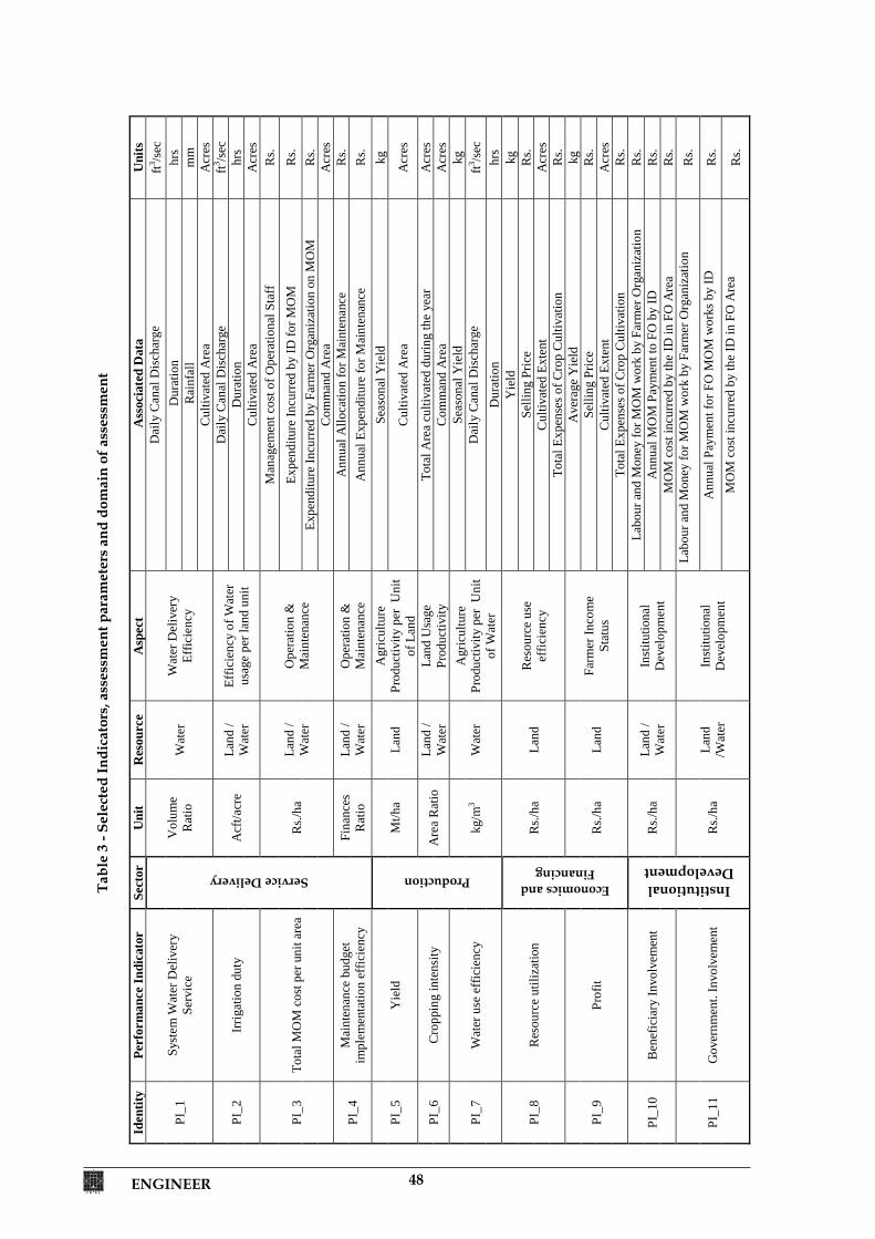
ENGINEER 48

Tabl

e 3

- Sel

ecte

d In

dica

tors

, ass

essm

ent p

aram

eter

s an

d do

mai

n of

ass

essm

ent

Id

entit

y Pe

rfor

man

ce In

dica

tor

Sect

or

Uni

t R

esou

rce

Asp

ect

Ass

ocia

ted

Dat

a U

nits

PI_1

Sy

stem

Wat

er D

eliv

ery

Serv

ice

Service Delivery

Vol

ume

Rat

io

Wat

er

Wat

er D

eliv

ery

Effic

ienc

y

Dai

ly C

anal

Dis

char

ge

ft3 /sec

D

urat

ion

hrs

Rai

nfal

l m

m

Cul

tivat

ed A

rea

Acr

es

PI_2

Ir

rigat

ion

duty

A

cft/a

cre

Land

/ W

ater

Ef

ficie

ncy

of W

ater

us

age

per l

and

unit

Dai

ly C

anal

Dis

char

ge

ft3 /sec

D

urat

ion

hrs

Cul

tivat

ed A

rea

Acr

es

PI_3

To

tal M

OM

cos

t per

uni

t are

a R

s./ha

La

nd /

Wat

er

Ope

ratio

n &

M

aint

enan

ce

Man

agem

ent c

ost o

f Ope

ratio

nal S

taff

R

s. Ex

pend

iture

Incu

rred

by

ID fo

r MO

M

Rs.

Expe

nditu

re In

curr

ed b

y Fa

rmer

Org

aniz

atio

n on

MO

M

Rs.

Com

man

d A

rea

Acr

es

PI_4

M

aint

enan

ce b

udge

t im

plem

enta

tion

effic

ienc

y Fi

nanc

es

Rat

io

Land

/ W

ater

O

pera

tion

&

Mai

nten

ance

A

nnua

l Allo

catio

n fo

r Mai

nten

ance

R

s. A

nnua

l Exp

endi

ture

for M

aint

enan

ce

Rs.

PI_5

Y

ield

Production

Mt/h

a La

nd

Agr

icul

ture

Pr

oduc

tivity

per

Uni

t of

Lan

d

Seas

onal

Yie

ld

kg

Cul

tivat

ed A

rea

Acr

es

PI_6

C

ropp

ing

inte

nsity

A

rea

Rat

io

Land

/ W

ater

La

nd U

sage

Pr

oduc

tivity

To

tal A

rea

culti

vate

d du

ring

the

year

A

cres

C

omm

and

Are

a A

cres

PI_7

W

ater

use

effi

cien

cy

kg/m

3 W

ater

A

gric

ultu

re

Prod

uctiv

ity p

er U

nit

of W

ater

Seas

onal

Yie

ld

kg

Dai

ly C

anal

Dis

char

ge

ft3 /sec

D

urat

ion

hrs

PI_8

R

esou

rce

utili

zatio

n

Economics and Financing

Rs./

ha

Land

R

esou

rce

use

effic

ienc

y

Yie

ld

kg

Selli

ng P

rice

Rs.

Cul

tivat

ed E

xten

t A

cres

To

tal E

xpen

ses o

f Cro

p C

ultiv

atio

n R

s.

PI_9

Pr

ofit

Rs./

ha

Land

Fa

rmer

Inco

me

Stat

us

Ave

rage

Yie

ld

kg

Selli

ng P

rice

Rs.

Cul

tivat

ed E

xten

t A

cres

To

tal E

xpen

ses o

f Cro

p C

ultiv

atio

n R

s.

PI_1

0 B

enef

icia

ry In

volv

emen

t

Institutional Development

Rs./

ha

Land

/ W

ater

In

stitu

tiona

l D

evel

opm

ent

Labo

ur a

nd M

oney

for M

OM

wor

k by

Far

mer

Org

aniz

atio

n R

s. A

nnua

l MO

M P

aym

ent t

o FO

by

ID

Rs.

MO

M c

ost i

ncur

red

by th

e ID

in F

O A

rea

Rs.

PI_1

1 G

over

nmen

t. In

volv

emen

t R

s./ha

La

nd

/Wat

er

Inst

itutio

nal

Dev

elop

men

t

Labo

ur a

nd M

oney

for M

OM

wor

k by

Far

mer

Org

aniz

atio

n R

s. A

nnua

l Pay

men

t for

FO

MO

M w

orks

by

ID

Rs.

MO

M c

ost i

ncur

red

by th

e ID

in F

O A

rea

Rs.

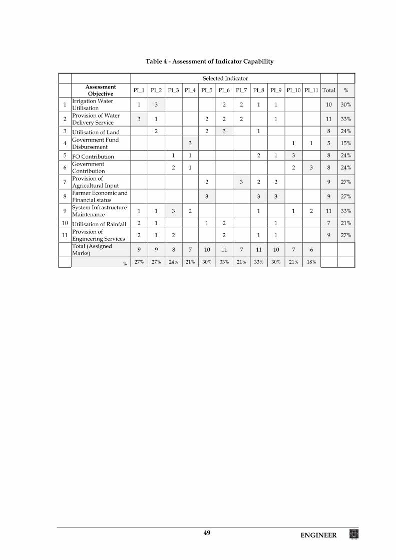
49 ENGINEER

Table 4 - Assessment of Indicator Capability

Selected Indicator

Assessment Objective PI_1 PI_2 PI_3 PI_4 PI_5 PI_6 PI_7 PI_8 PI_9 PI_10 PI_11 Total %

1 Irrigation Water Utilisation 1 3 2 2 1 1 10 30%

2 Provision of Water Delivery Service 3 1 2 2 2 1 11 33%

3 Utilisation of Land 2 2 3 1 8 24%

4 Government Fund Disbursement 3 1 1 5 15%

5 FO Contribution 1 1 2 1 3 8 24%

6 Government Contribution 2 1 2 3 8 24%

7 Provision of Agricultural Input 2 3 2 2 9 27%

8 Farmer Economic and Financial status 3 3 3 9 27%

9 System Infrastructure Maintenance 1 1 3 2 1 1 2 11 33%

10 Utilisation of Rainfall 2 1 1 2 1 7 21%

11 Provision of Engineering Services 2 1 2 2 1 1 9 27%

Total (Assigned Marks) 9 9 8 7 10 11 7 11 10 7 6

% 27% 27% 24% 21% 30% 33% 21% 33% 30% 21% 18%

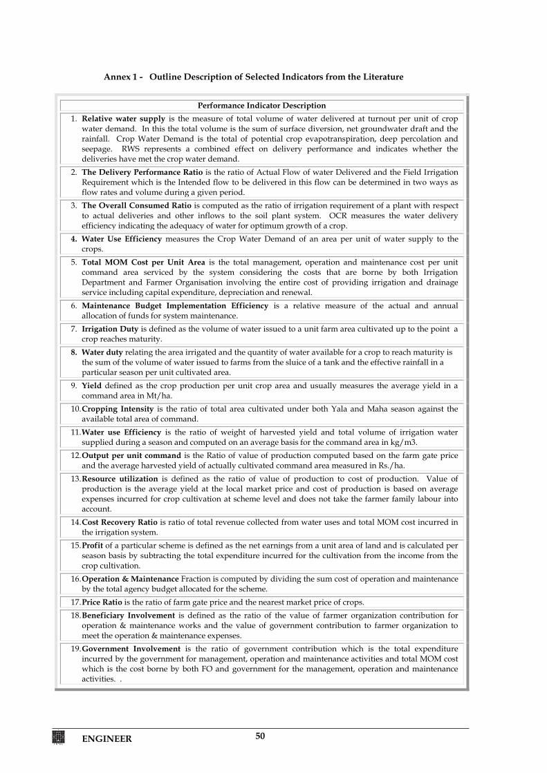
ENGINEER 50

Annex 1 - Outline Description of Selected Indicators from the Literature

Performance Indicator Description 1. Relative water supply is the measure of total volume of water delivered at turnout per unit of crop

water demand. In this the total volume is the sum of surface diversion, net groundwater draft and the rainfall. Crop Water Demand is the total of potential crop evapotranspiration, deep percolation and seepage. RWS represents a combined effect on delivery performance and indicates whether the deliveries have met the crop water demand.

2. The Delivery Performance Ratio is the ratio of Actual Flow of water Delivered and the Field Irrigation Requirement which is the Intended flow to be delivered in this flow can be determined in two ways as flow rates and volume during a given period.

3. The Overall Consumed Ratio is computed as the ratio of irrigation requirement of a plant with respect to actual deliveries and other inflows to the soil plant system. OCR measures the water delivery efficiency indicating the adequacy of water for optimum growth of a crop.

4. Water Use Efficiency measures the Crop Water Demand of an area per unit of water supply to the crops.

5. Total MOM Cost per Unit Area is the total management, operation and maintenance cost per unit command area serviced by the system considering the costs that are borne by both Irrigation Department and Farmer Organisation involving the entire cost of providing irrigation and drainage service including capital expenditure, depreciation and renewal.

6. Maintenance Budget Implementation Efficiency is a relative measure of the actual and annual allocation of funds for system maintenance.

7. Irrigation Duty is defined as the volume of water issued to a unit farm area cultivated up to the point a crop reaches maturity.

8. Water duty relating the area irrigated and the quantity of water available for a crop to reach maturity is the sum of the volume of water issued to farms from the sluice of a tank and the effective rainfall in a particular season per unit cultivated area.

9. Yield defined as the crop production per unit crop area and usually measures the average yield in a command area in Mt/ha.

10. Cropping Intensity is the ratio of total area cultivated under both Yala and Maha season against the available total area of command.

11. Water use Efficiency is the ratio of weight of harvested yield and total volume of irrigation water supplied during a season and computed on an average basis for the command area in kg/m3.

12. Output per unit command is the Ratio of value of production computed based on the farm gate price and the average harvested yield of actually cultivated command area measured in Rs./ha.

13. Resource utilization is defined as the ratio of value of production to cost of production. Value of production is the average yield at the local market price and cost of production is based on average expenses incurred for crop cultivation at scheme level and does not take the farmer family labour into account.

14. Cost Recovery Ratio is ratio of total revenue collected from water uses and total MOM cost incurred in the irrigation system.

15. Profit of a particular scheme is defined as the net earnings from a unit area of land and is calculated per season basis by subtracting the total expenditure incurred for the cultivation from the income from the crop cultivation.

16. Operation & Maintenance Fraction is computed by dividing the sum cost of operation and maintenance by the total agency budget allocated for the scheme.

17. Price Ratio is the ratio of farm gate price and the nearest market price of crops. 18. Beneficiary Involvement is defined as the ratio of the value of farmer organization contribution for

operation & maintenance works and the value of government contribution to farmer organization to meet the operation & maintenance expenses.

19. Government Involvement is the ratio of government contribution which is the total expenditure incurred by the government for management, operation and maintenance activities and total MOM cost which is the cost borne by both FO and government for the management, operation and maintenance activities. .

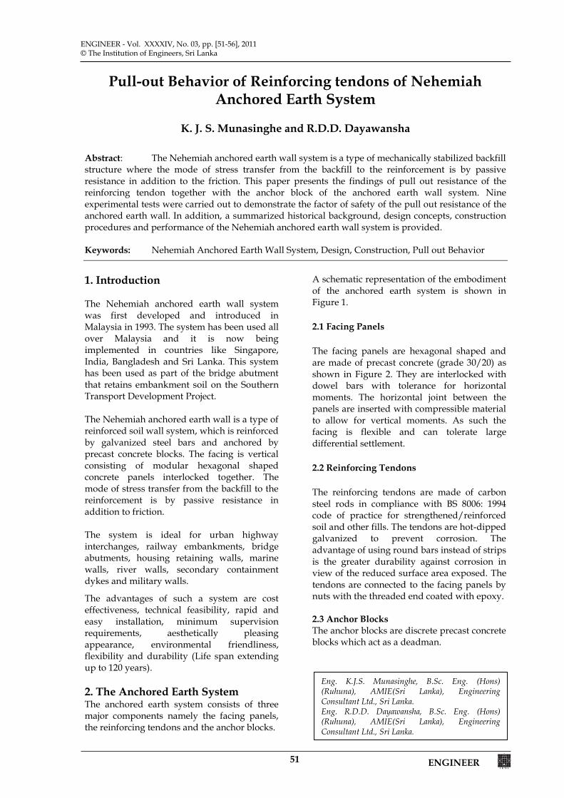
51 ENGINEER

ENGINEER - Vol. XXXXIV, No. 03, pp. [51-56], 2011© The Institution of Engineers, Sri Lanka

Pull-out Behavior of Reinforcing tendons of Nehemiah Anchored Earth System

K. J. S. Munasinghe and R.D.D. Dayawansha

Abstract: The Nehemiah anchored earth wall system is a type of mechanically stabilized backfill structure where the mode of stress transfer from the backfill to the reinforcement is by passive resistance in addition to the friction. This paper presents the findings of pull out resistance of the reinforcing tendon together with the anchor block of the anchored earth wall system. Nine experimental tests were carried out to demonstrate the factor of safety of the pull out resistance of the anchored earth wall. In addition, a summarized historical background, design concepts, construction procedures and performance of the Nehemiah anchored earth wall system is provided. Keywords: Nehemiah Anchored Earth Wall System, Design, Construction, Pull out Behavior

1. Introduction The Nehemiah anchored earth wall system was first developed and introduced in Malaysia in 1993. The system has been used all over Malaysia and it is now being implemented in countries like Singapore, India, Bangladesh and Sri Lanka. This system has been used as part of the bridge abutment that retains embankment soil on the Southern Transport Development Project. The Nehemiah anchored earth wall is a type of reinforced soil wall system, which is reinforced by galvanized steel bars and anchored by precast concrete blocks. The facing is vertical consisting of modular hexagonal shaped concrete panels interlocked together. The mode of stress transfer from the backfill to the reinforcement is by passive resistance in addition to friction. The system is ideal for urban highway interchanges, railway embankments, bridge abutments, housing retaining walls, marine walls, river walls, secondary containment dykes and military walls.

The advantages of such a system are cost effectiveness, technical feasibility, rapid and easy installation, minimum supervision requirements, aesthetically pleasing appearance, environmental friendliness, flexibility and durability (Life span extending up to 120 years). 2. The Anchored Earth System The anchored earth system consists of three major components namely the facing panels, the reinforcing tendons and the anchor blocks.

A schematic representation of the embodiment of the anchored earth system is shown in Figure 1. 2.1 Facing Panels The facing panels are hexagonal shaped and are made of precast concrete (grade 30/20) as shown in Figure 2. They are interlocked with dowel bars with tolerance for horizontal moments. The horizontal joint between the panels are inserted with compressible material to allow for vertical moments. As such the facing is flexible and can tolerate large differential settlement. 2.2 Reinforcing Tendons The reinforcing tendons are made of carbon steel rods in compliance with BS 8006: 1994 code of practice for strengthened/reinforced soil and other fills. The tendons are hot-dipped galvanized to prevent corrosion. The advantage of using round bars instead of strips is the greater durability against corrosion in view of the reduced surface area exposed. The tendons are connected to the facing panels by nuts with the threaded end coated with epoxy. 2.3 Anchor Blocks The anchor blocks are discrete precast concrete blocks which act as a deadman.

Eng. K.J.S. Munasinghe, B.Sc. Eng. (Hons) (Ruhuna), AMIE(Sri Lanka), Engineering Consultant Ltd., Sri Lanka. Eng. R.D.D. Dayawansha, B.Sc. Eng. (Hons) (Ruhuna), AMIE(Sri Lanka), Engineering Consultant Ltd., Sri Lanka.

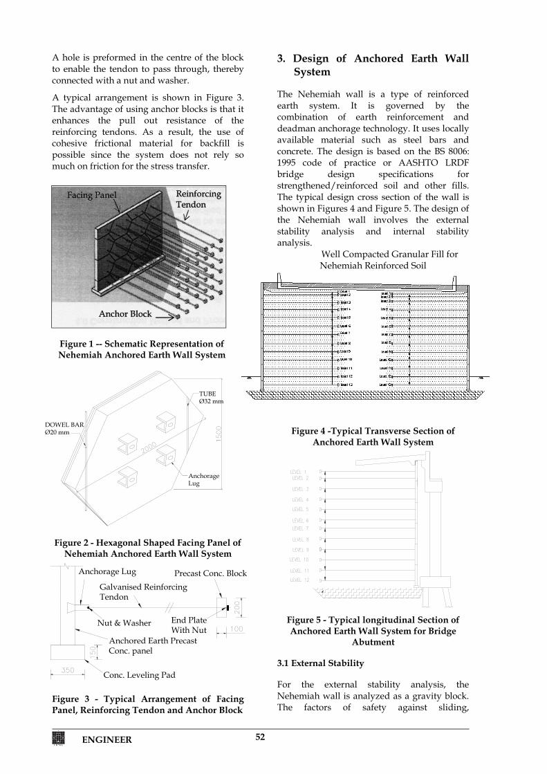
ENGINEER 52

End PlateWith Nut

Conc. Leveling Pad

Anchored Earth PrecastConc. panel

Anchorage Lug

Nut & Washer

Galvanised ReinforcingTendon

Precast Conc. Block

A hole is preformed in the centre of the block to enable the tendon to pass through, thereby connected with a nut and washer.

A typical arrangement is shown in Figure 3. The advantage of using anchor blocks is that it enhances the pull out resistance of the reinforcing tendons. As a result, the use of cohesive frictional material for backfill is possible since the system does not rely so much on friction for the stress transfer.

Figure 1 -- Schematic Representation of Nehemiah Anchored Earth Wall System

Figure 2 - Hexagonal Shaped Facing Panel of

Nehemiah Anchored Earth Wall System Figure 3 - Typical Arrangement of Facing Panel, Reinforcing Tendon and Anchor Block

3. Design of Anchored Earth Wall System

The Nehemiah wall is a type of reinforced earth system. It is governed by the combination of earth reinforcement and deadman anchorage technology. It uses locally available material such as steel bars and concrete. The design is based on the BS 8006: 1995 code of practice or AASHTO LRDF bridge design specifications for strengthened/reinforced soil and other fills. The typical design cross section of the wall is shown in Figures 4 and Figure 5. The design of the Nehemiah wall involves the external stability analysis and internal stability analysis.

Well Compacted Granular Fill for Nehemiah Reinforced Soil

Figure 4 -Typical Transverse Section of Anchored Earth Wall System

Figure 5 - Typical longitudinal Section of Anchored Earth Wall System for Bridge

Abutment 3.1 External Stability For the external stability analysis, the Nehemiah wall is analyzed as a gravity block. The factors of safety against sliding,

DOWEL BARØ20 mm

TUBEØ32 mm

AnchorageLug

53 ENGINEER

overturning and bearing are checked; designed to ensure that they are adequate. The global analysis and the geotechnical analysis are also external stability analysis. They are not described in this paper. 3.2 Internal Stability The internal stability analysis involves checks to ensure that the factors of safety against tensile strength and pull out failure of all the reinforcing tendons are adequate. 3.2.1 Tensile Failure In the design, it is important that the number and size of the reinforcing tendons are adequately provided so that the tension developed in the tendons is always less than the allowable tensile strength of all the tendons. The tensions in the reinforcing tendons [4] are computed as follows: Where, Ti = Tension developed in the reinforcing tendon at ith levels K = Coefficient of earth pressure within the reinforced block Sv = Vertical spacing of the tendons

v = Vertical stress acting on the ith level of the tendons according to the Meyerhof pressure distribution 3.2.2 Pull out Failure The ultimate pull out resistance of the reinforcing tendons is the sum of the shaft frictional resistance and the anchor capacity of the anchor block. The shaft resistance is determined by the friction developed between the backfill and the effective length of the tendon [7] Which is shown in Figure 6.

Figure 6 - Effective Length of Reinforcing Tendons – Le

The shaft resistance is computed as follows:

Where, Fs = Shaft resistance = Coefficient of friction Ø = Angle of Internal friction of the backfill d = Diameter of the tendon Le = Effective shaft length The anchor capacity [7] is computed as follows: Where, Pa = Passive resistance of the backfill in front of the anchor block Kp = Coefficient of passive earth pressure h = Height of the anchor block w = Width of the anchor block Hence, the total pull out resistance is given as follows: The factor of safety for pull out resistance must be larger than or equal to unity. It is computed as follows. Where, Pr = Ultimate pull out resistance Ø = Resistance factor for pull out resistance, which can be take as 0.9 Tdesign = Design working load 4. Construction of Nehemiah

Anchored Earth Wall System The construction sequence shall start with site preparation before wall construction. It is explained under the following headings. 4.1 Site Preparation The first step in the construction was to remove the unsuitable subsoil material or any weak material with debris and replace it with compacted granular material. Once the sub soil was strengthened, the leveling pad was cast at base level. Unreinforced grade 20/20 concrete was used. After the site preparation was completed, the wall erection can be commenced.

1............................................VVSKTi

2..............................tan VeS LdF

3........................................4 vpa whKP

4..............................................aSr PFP

5..PrtandesignT

cesisoutPullforFOS Re

Rankine Failure Plane

(45 - Ø/2)

ActiveZone

ResistantZone

Le

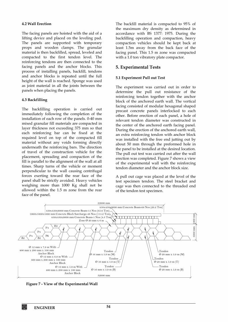
ENGINEER 54

B2P4

P4P4

H2

B2P4

22000 mm

32000 mm

450x450x9000 mm Concrete Beam-06 Nos (26.2 Ton)450x450x9000 mm Concrete Beam-15 Nos (65.6 Ton)

1000x1000x1000 mm Concrete Block Surcharge-48 Nos (115.2 Ton)450x450x9000 mm Concrete Beam-1 Nos (4.3 Ton)

Zone Ø 20 mm x 6 m

1900

mm

Ø 12 mm x 7.9 m With400 mm x 200 mm x 100 mm

Anchor BlockØ 12 mm x 6.9 m With

400 mm x 200 mm x 100 mmAnchor Block

Ø 12 mm x 5.9 m With400 mm x 200 mm x 100 mm

Anchor Block

TendonØ 16 mm x 5.9 m (M)

TendonØ 16 mm x 5.9 m (T)

TendonØ 20 mm x 5.9 m (M)

TendonØ 20 mm x 5.9 m (T)

TendonØ 20 mm x 5.9 m (B)

TendonØ 16 mm x 5.9 m (B)

3000

mm

4.2 Wall Erection The facing panels are hoisted with the aid of a lifting device and placed on the leveling pad. The panels are supported with temporary props and wooden clamps. The granular material is then backfilled, spread, leveled and compacted to the first tendon level. The reinforcing tendons are then connected to the facing panels and the anchor blocks. This process of installing panels, backfill, tendons and anchor blocks is repeated until the full height of the wall is reached. Sponge was used as joint material in all the joints between the panels when placing the panels. 4.3 Backfilling The backfilling operation is carried out immediately following the completion of the installation of each row of the panels. 0-40 mm mixed granular fill materials are compacted in layer thickness not exceeding 375 mm so that each reinforcing bar can be fixed at the required level on top of the compacted fill material without any voids forming directly underneath the reinforcing bars. The direction of travel of the construction vehicle for the placement, spreading and compaction of the fill is parallel to the alignment of the wall at all times. Sharp turns of the vehicle or moment perpendicular to the wall causing centrifugal forces exerting toward the rear face of the panel shall be strictly avoided. Heavy vehicles weighing more than 1000 Kg shall not be allowed within the 1.5 m zone from the rear face of the panel.

Figure 7 - View of the Experimental Wall

The backfill material is compacted to 95% of the maximum dry density as determined in accordance with BS 1377: 1975. During the backfilling operation and compaction, heavy compaction vehicles should be kept back at least 1.5m away from the back face of the facing panel. This 1.5 m zone was compacted with a 1.0 ton vibratory plate compactor. 5. Experimental Tests

5.1 Experiment Pull out Test The experiment was carried out in order to determine the pull out resistance of the reinforcing tendon together with the anchor block of the anchored earth wall. The vertical facing consisted of modular hexagonal shaped precast concrete panels interlocked to each other. Before erection of each panel, a hole of relevant tendon diameter was constructed in the center of the anchored earth facing panel. During the erection of the anchored earth wall, an extra reinforcing tendon with anchor block was installed with the free end jutting out by about 50 mm through the preformed hole in the panel to be installed at the desired location. The pull out test was carried out after the wall erection was completed. Figure 7 shows a view of the experimental wall with the reinforcing tendon diameter and the anchor block size. A pull out cage was placed at the level of the test specimen tendon. The steel bracket and cage was then connected to the threaded end of the tendon test specimen.

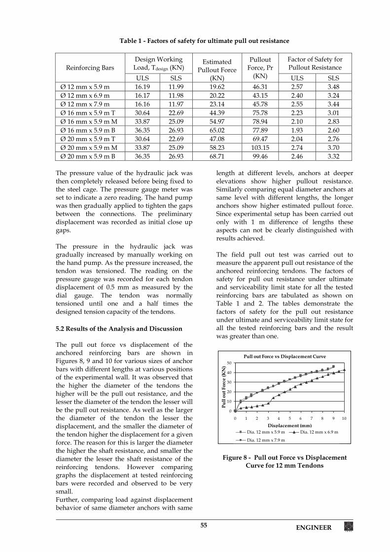
55 ENGINEER

Table 1 - Factors of safety for ultimate pull out resistance

Reinforcing Bars Design Working Load, Tdesign (KN)

Estimated Pullout Force

(KN)

Pullout Force, Pr

(KN)

Factor of Safety for Pullout Resistance

ULS SLS ULS SLS Ø 12 mm x 5.9 m 16.19 11.99 19.62 46.31 2.57 3.48 Ø 12 mm x 6.9 m 16.17 11.98 20.22 43.15 2.40 3.24 Ø 12 mm x 7.9 m 16.16 11.97 23.14 45.78 2.55 3.44 Ø 16 mm x 5.9 m T 30.64 22.69 44.39 75.78 2.23 3.01 Ø 16 mm x 5.9 m M 33.87 25.09 54.97 78.94 2.10 2.83 Ø 16 mm x 5.9 m B 36.35 26.93 65.02 77.89 1.93 2.60 Ø 20 mm x 5.9 m T 30.64 22.69 47.08 69.47 2.04 2.76 Ø 20 mm x 5.9 m M 33.87 25.09 58.23 103.15 2.74 3.70 Ø 20 mm x 5.9 m B 36.35 26.93 68.71 99.46 2.46 3.32

The pressure value of the hydraulic jack was then completely released before being fixed to the steel cage. The pressure gauge meter was set to indicate a zero reading. The hand pump was then gradually applied to tighten the gaps between the connections. The preliminary displacement was recorded as initial close up gaps. The pressure in the hydraulic jack was gradually increased by manually working on the hand pump. As the pressure increased, the tendon was tensioned. The reading on the pressure gauge was recorded for each tendon displacement of 0.5 mm as measured by the dial gauge. The tendon was normally tensioned until one and a half times the designed tension capacity of the tendons. 5.2 Results of the Analysis and Discussion The pull out force vs displacement of the anchored reinforcing bars are shown in Figures 8, 9 and 10 for various sizes of anchor bars with different lengths at various positions of the experimental wall. It was observed that the higher the diameter of the tendons the higher will be the pull out resistance, and the lesser the diameter of the tendon the lesser will be the pull out resistance. As well as the larger the diameter of the tendon the lesser the displacement, and the smaller the diameter of the tendon higher the displacement for a given force. The reason for this is larger the diameter the higher the shaft resistance, and smaller the diameter the lesser the shaft resistance of the reinforcing tendons. However comparing graphs the displacement at tested reinforcing bars were recorded and observed to be very small. Further, comparing load against displacement behavior of same diameter anchors with same

length at different levels, anchors at deeper elevations show higher pullout resistance. Similarly comparing equal diameter anchors at same level with different lengths, the longer anchors show higher estimated pullout force. Since experimental setup has been carried out only with 1 m difference of lengths these aspects can not be clearly distinguished with results achieved. The field pull out test was carried out to measure the apparent pull out resistance of the anchored reinforcing tendons. The factors of safety for pull out resistance under ultimate and serviceability limit state for all the tested reinforcing bars are tabulated as shown on Table 1 and 2. The tables demonstrate the factors of safety for the pull out resistance under ultimate and serviceability limit state for all the tested reinforcing bars and the result was greater than one.

Pull out Force vs Displacement Curve

0

10

20

30

40

50

0 1 2 3 4 5 6 7 8 9 10

Displacement (mm)

Pull

out F

orce

(KN

)

Dia. 12 mm x 5.9 m Dia. 12 mm x 6.9 m

Dia. 12 mm x 7.9 m

Figure 8 - Pull out Force vs Displacement Curve for 12 mm Tendons

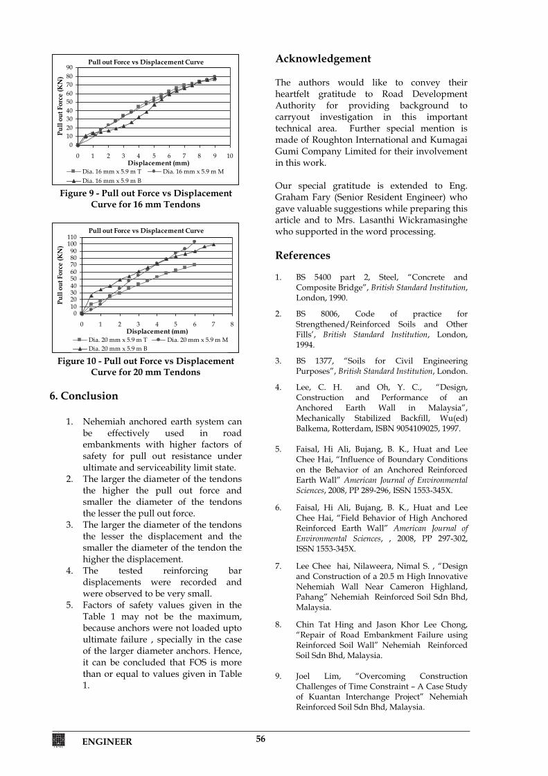
ENGINEER 56

Pull out Force vs Displacement Curve

0102030405060708090

0 1 2 3 4 5 6 7 8 9 10Displacement (mm)

Pull

out F

orce

(KN

)

Dia. 16 mm x 5.9 m T Dia. 16 mm x 5.9 m MDia. 16 mm x 5.9 m B

Figure 9 - Pull out Force vs Displacement Curve for 16 mm Tendons

Pull out Force vs Displacement Curve

0102030405060708090

100110

0 1 2 3 4 5 6 7 8Displacement (mm)

Pull

out F

orce

(KN

)

Dia. 20 mm x 5.9 m T Dia. 20 mm x 5.9 m MDia. 20 mm x 5.9 m B

Figure 10 - Pull out Force vs Displacement Curve for 20 mm Tendons

6. Conclusion

1. Nehemiah anchored earth system can be effectively used in road embankments with higher factors of safety for pull out resistance under ultimate and serviceability limit state.

2. The larger the diameter of the tendons the higher the pull out force and smaller the diameter of the tendons the lesser the pull out force.

3. The larger the diameter of the tendons the lesser the displacement and the smaller the diameter of the tendon the higher the displacement.

4. The tested reinforcing bar displacements were recorded and were observed to be very small.

5. Factors of safety values given in the Table 1 may not be the maximum, because anchors were not loaded upto ultimate failure , specially in the case of the larger diameter anchors. Hence, it can be concluded that FOS is more than or equal to values given in Table 1.

Acknowledgement The authors would like to convey their heartfelt gratitude to Road Development Authority for providing background to carryout investigation in this important technical area. Further special mention is made of Roughton International and Kumagai Gumi Company Limited for their involvement in this work. Our special gratitude is extended to Eng. Graham Fary (Senior Resident Engineer) who gave valuable suggestions while preparing this article and to Mrs. Lasanthi Wickramasinghe who supported in the word processing. References 1. BS 5400 part 2, Steel, “Concrete and

Composite Bridge”, British Standard Institution, London, 1990.

2. BS 8006, Code of practice for Strengthened/Reinforced Soils and Other Fills’, British Standard Institution, London, 1994.

3. BS 1377, “Soils for Civil Engineering Purposes”, British Standard Institution, London.

4. Lee, C. H. and Oh, Y. C., “Design, Construction and Performance of an Anchored Earth Wall in Malaysia”, Mechanically Stabilized Backfill, Wu(ed) Balkema, Rotterdam, ISBN 9054109025, 1997.

5. Faisal, Hi Ali, Bujang, B. K., Huat and Lee

Chee Hai, “Influence of Boundary Conditions on the Behavior of an Anchored Reinforced Earth Wall” American Journal of Environmental Sciences, 2008, PP 289-296, ISSN 1553-345X.

6. Faisal, Hi Ali, Bujang, B. K., Huat and Lee Chee Hai, “Field Behavior of High Anchored Reinforced Earth Wall” American Journal of Environmental Sciences, , 2008, PP 297-302, ISSN 1553-345X.

7. Lee Chee hai, Nilaweera, Nimal S. , “Design and Construction of a 20.5 m High Innovative Nehemiah Wall Near Cameron Highland, Pahang” Nehemiah Reinforced Soil Sdn Bhd, Malaysia.

8. Chin Tat Hing and Jason Khor Lee Chong, “Repair of Road Embankment Failure using Reinforced Soil Wall” Nehemiah Reinforced Soil Sdn Bhd, Malaysia.

9. Joel Lim, “Overcoming Construction

Challenges of Time Constraint – A Case Study of Kuantan Interchange Project” Nehemiah Reinforced Soil Sdn Bhd, Malaysia.

57 ENGINEER

ENGINEER - Vol. XXXXIV, No. 03, pp. [57-66], 2011© The Institution of Engineers, Sri Lanka

Economic Analysis of Water Infrastructure: Have We Got It Right?

Bhadranie Thoradeniya, Malik Ranasinghe, N T S Wijesekara

Abstract: The paper describes shortcomings of the general economic analysis procedure adopted in water infrastructure development projects in Sri Lanka. As a case study an application of the ‘Educated Trade-off’ framework in the Ma Oya river basin is used to illustrate the shortcomings of general economic analysis procedure. This framework facilitates the systematic identification of resource uses and the possible range of environmental and social impacts by the water infrastructure project, through the involvement (consultation and participation) of key stakeholders. The study revealed two types of shortcomings that result in erroneous economic indicators: first, the lack of a competent process to establish the baseline situation leading to non-inclusion of some important social and environmental impacts, both positive and negative, by the project and, second, deviations from reasonable practices either due to negligence or on purposes that give decision makers optimistic data which could result in questionable decisions. Keywords: economic analysis, water infrastructure development projects, educated trade-off, stakeholder consultation, natural resources

1. Introduction Water infrastructure development can be considered as a production process as the purpose of production is to convert a set of inputs (e.g. river flow, concrete, steel and other building materials) to a set of outputs (e.g. irrigation, water supply, and hydropower generation projects). This justifies the application of production functions, cost benefit analysis and other economic analysis to water resource infrastructure development [20]. In the economic analysis of an infrastructure project, the total value of the resource has to be considered to maximise the efficiency. The total value of a resource consists of its use and non-use values. The basic measures of use and non-use values are maximum willingness to pay (WTP) to prevent environmental damage or realise an economic-environmental benefit; and/or minimum willingness to accept (WTA) compensation for accepting a specific degradation in environmental quality [1]. Non-availability of a systematic approach to establish the baseline situation of the full range of use and non-use values of the resources is a key deficiency associated with the procedure generally adopted for economic analysis of water infrastructure projects especially in river development work. Inadequate efforts to include the values of full range of social and environmental impacts due to the development

project aggravate the situation. This practice could be due to lack of knowledge, negligence or on purpose. The objective of this paper is to present a case study on proposed Yatimahana multi-purpose balancing reservoir which is a water infrastructure project on Ma Oya in order to: a) highlight deviations in economic analysis

from reasonable practices either due to negligence or on purpose, and

b) address the above deficiencies through the application of an ‘Educated Trade-offs’ framework [16], [17].

The ‘Educated Trade-offs’ framework developed by Thoradeniya [17] is a decision-making tool to facilitate trade-offs between different resource uses by educating the stakeholders on the combined economic value (economic estimates and environmental and social costs) of each resource use sector.

Eng. Dr. (Mrs.) Bhadranie Thoradeniya, AMIE(Sri Lanka), PhD, Head, Division of Civil EngineeringTechnology, Institute of Technology, University of Moratuwa Eng. (Prof.) Malik Ranasinghe, B.Sc. Eng. Hons, Int. PEng., C.Eng., FIE(Sri Lanka), M.A.Sc., PhD, Professor in Civil Engineering and the Vice-Chancellor of the University of Moratuwa Eng. (Prof.) N.T.S. Wijesekera, B.Sc. Eng. (Hons), C.Eng., FIE(Sri Lanka), MICE(UK), PG. Dip., M.Eng., D.Eng., Senior Professor in Civil Engineering, University of Moratuwa.

ENGINEER 58

The framework consists of five steps. The first step identifies the stakeholders and the uses/issues of the natural resources in the total area impacted by the project, through the systematic consultation of stakeholder groups. The critical bounds of the technical requirements of the resource uses and issues identified in step one are then estimated in step two. The economic value and the environmental (including social) costs of the respective critical bound of the technical requirements are estimated in the third and the fourth steps. The fifth step combines the economic estimates and the environmental and social costs of critical bounds, to form the basis for ‘Educated Trade-offs’ for stakeholder consultations [16], [17]. This paper describes the application of the step 1 of the above framework briefly and steps 3 and 4 in detail, which are relevant to the objectives of this paper. The case study application highlighted two main factors; a) the erroneous approaches in the methodologies employed by the project analysts in performing economic analysis of the water infrastructure project b) the inability of general approaches to capture ground realities in the economic analysis. Both the above factors resulted in obtaining wrong economic indicators that would mislead the decision makers. The next section presents an overview of the economic theories that are used for these analyses. The third section describes the case study (the proposed Yatimahana reservoir) and the baseline scenario. The fourth section presents estimates of combined economic values of the water infrastructure project. The conclusions are given in the fifth section. 2. Overview of the Economic

Theories 2.1 Economic Indicators Economic Net Present Value (EcoNPV) and Economic Internal Rate of Return (EIRR) analyses are frequently used to determine the difference in economic benefits and economic costs of a water infrastructure project. The Present Value (PV) of net benefits and costs over time is its value today, usually represented as time zero in a cash flow diagram. In other words, it is the value obtained by discounting the benefits and costs separately for each year over time at a constant

discount rate and, throughout the assumed life of a development project [11]. Then, the fundamental relationship to determine the Economic Net Present Value (EcoNPV) of a resource use can be expressed as;

n

iiii

rCB

EcoNPV0 )1(

[2.1]

Where Bi is the annual economic benefits from the use of resource at the ith year and Ci is the economic cost of the resource use at the ith year. ‘n’ is the duration of the study period and ‘r’ is the discount rate [17]. Economic Internal Rate of Return (EIRR) is the most often cited method for comparing alternatives in development projects. The EIRR analysis calculates the return from the development project as a non-dimensional measure. Present value formulations are the foundations for EIRR calculation as the EIRR is calculated by equating EcoNPV given in equation 2.1 to zero and solving for the discount rate that allows the equality [11]. Therefore, Internal Rate of Return (IRR) is generally defined as the rate at which PV of costs is equal to the PV of benefits, or the rate at which the NPV is equal to zero. The IRR preference (ranking) for an alternative always agrees with that of the NPV preference for projects, which are economically independent of one another (i.e. the selection of a particular project does not preclude the choice of the other). When the alternatives are mutually exclusive, there can be reversal of rankings. Alternatives are mutually exclusive when the selection of one alternative eliminates the opportunity to invest in any of the others. Most problems in development projects normally fit into this category because a single course of action is sought to solve a particular, often urgent, problem. When the best alternative is determined, the problem is theoretically resolved by implementing the indicated course of action [13]. In choosing between alternatives (i.e. different resource uses), the criterion is to select the one that maximizes EcoNPV. For instance, an EcoNPV of Rs. Z means that the PV of the alternative (resource use) is Rs. Z greater than on an investment of similar size that produces a rate of return equal to the discount rate or the Minimum Acceptable Rate of Return (MARR).

59 ENGINEER

A negative PV means that the alternative does not satisfy the rate of return requirement, as MARR reflects the opportunity cost of capital. In other words, the possible return the economy would obtain is lower on the same amount of capital than if invested elsewhere at MARR, assuming that the risks are similar for both investment alternatives [11, 12]. 2.2 Financial Analysis The starting point of an economic analysis of a resource use is the financial analysis of that resource use. The financial analysis measures the receipts (benefits) and payments (costs) relevant to the investors or owners of the resource/project. It is a tool that provides investors with the information required to decide whether to undertake an investment. Hence, the objectives of the financial analysis are to determine, analyse and interpret all financial consequences that may be relevant to and significant for investment and financing decisions [11]. The financial analysis of a resource use/project is typically carried out at market prices prevailing at the time of the analysis [7]. The estimates for costs and benefits (receipts) are therefore in terms of prevailing market prices. Taxes and subsidies (transfer payments), foreign exchange distortions, monopoly rents, and externalities influence market prices. Market distortions cause market prices to diverge from economic prices [7]. 2.3 Economic Analysis According to Jenkins and Harberger [7], for inputs, market prices would reveal the productive value of an item in its next best use. The market prices of an output would signal the level at which the consumer's marginal WTP for an item just equals the cost of producing that item (marginal cost). Instead, market distortions cause market prices to diverge from "economic prices." For example, taxes increase prices and reduce demand. The effect of subsidies is opposite [7], [2]. The financial analysis relies on cash flow techniques to compare and analyse the estimated receipts (benefits) and costs. An economic analysis is of exactly the same nature as a financial analysis, except in the case of an economic analysis, the benefits and costs are measured from the point of view of the economy [7]. Instead of relying solely on cash

flow techniques to measure benefits and costs as in the case of the financial analysis, economic valuation requires the use of economic techniques of measurement. Then, the merit of a resource use is assessed with regard to the impact that use has on the efficiency of the economy as a whole [7]. The market prices are adjusted to reflect the opportunity cost (or shadow price) of goods and services. Then, the cost to society of the project is measured in terms of forgone marginal products of inputs, had they been used in the next best alternative to the resource use. The outputs of the resource use are valued based on their demand price in the absence of market distortions [7]. Ideally, the price of every input and output should be adjusted so that “shadow prices” can be approximated. Once the shadow (economic) price is known, a conversion factor of the ratio of the economic price to the market price, is used to facilitate this adjustment. When the conversion factors are approximated, computer spreadsheet programs easily facilitate the transformation of the financial analysis to the economic analysis. Instead of replacing all financial values with economic values, financial values can be multiplied by the conversion factors to yield economic values [11], [4]. The complexity of finding the economic price depends on the nature of the good or service being considered. The third step of the ‘Educated Trade-off’ framework uses these reasoning to estimate the economic value of the water infrastructure project. 2.4 Extended Economic Analysis A negative outcome often linked with the water resources development is the environmental degradation that occurs due to the economic activities [10]. Inclusion of such costs (and benefits) in the water infrastructure project is the basis for the ‘Extended Economic Analysis.’ It is imperative to value such impacts to the environment in related decision making [8], [9], [6]. Birol et al. [3] defines the role of economic valuation techniques in the design of efficient, equitable and sustainable policies for water resources management in the face of environmental problems.

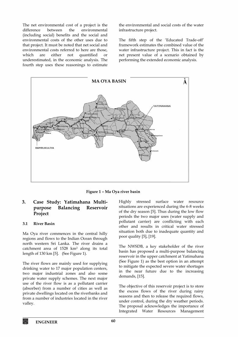
ENGINEER 60

The net environmental cost of a project is the difference between the environmental (including social) benefits and the social and environmental costs of the other uses due to that project. It must be noted that net social and environmental costs referred to here are those, which are either not quantified or underestimated, in the economic analysis. The fourth step uses these reasonings to estimate

the environmental and social costs of the water infrastructure project. The fifth step of the ‘Educated Trade-off’ framework estimates the combined value of the water infrastructure project. This in fact is the net present value of a scenario obtained by performing the extended economic analysis.

Figure 1 – Ma Oya river basin 3. Case Study: Yatimahana Multi-

purpose Balancing Reservoir Project

3.1 River Basin Ma Oya river commences in the central hilly regions and flows to the Indian Ocean through north western Sri Lanka. The river drains a catchment area of 1528 km2 along its total length of 130 km [5]. (See Figure 1). The river flows are mainly used for supplying drinking water to 17 major population centers, two major industrial zones and also some private water supply schemes. The next major use of the river flow is as a pollutant carrier (absorber) from a number of cities as well as private dwellings located on the riverbanks and from a number of industries located in the river valley.

Highly stressed surface water resource situations are experienced during the 6-8 weeks of the dry season [5]. Thus during the low flow periods the two major uses (water supply and pollutant carrier) are conflicting with each other and results in critical water stressed situation both due to inadequate quantity and poor quality [5], [19]. The NWSDB, a key stakeholder of the river basin has proposed a multi-purpose balancing reservoir in the upper catchment at Yatimahana (See Figure 1) as the best option in an attempt to mitigate the expected severe water shortages in the near future due to the increasing demands, [15]. The objective of this reservoir project is to store the excess flows of the river during rainy seasons and then to release the required flows, under control, during the dry weather periods. The proposal acknowledges the importance of Integrated Water Resources Management

MA OYA BASIN

61 ENGINEER

(IWRM) and has considered irrigation, industry and hydropower sectors in addition to the water supply and sanitation sector. Hydropower is proposed mainly as a strategy for achieving the economic viability of the reservoir project [15]. 3.2 Baseline Scenario The resource uses and issues of a river show a significant variation spatially and temporally. It is therefore vital to establish the baseline situation and the possible impacts by the water infrastructure project prior to engaging in economic analyses. The baseline situation should be established by carrying out systematic surveys covering the entire area that is expected to be impacted by the project. A main feature of the ‘Educated Trade-off’ framework is the establishment of the baseline scenario with regard to total value of the resource against the current practice of limiting the analyses mostly to direct use values. The first step of the ‘Educated Trade-off’ framework is developed on the premise that the establishment of the most accurate baseline situation for identifying the resource uses is through the bottom level (grass-root) stakeholder consultations. The methodology used for the identification of stakeholders and issues was to conduct sample surveys along the river banks at the smallest administrative unit (Grama Niladhari Division – GND) level. In this case study, the sample constituted of 427 stakeholders from 145 GNDs along both river banks from river estuary to Aranayake (a location upstream of the proposed reservoir), representing all sectors having a stake in the river including public administration, public and private institutions in river resource use sectors. It also included representatives of social, political, religious, and ethnic groups of public at grass-root level. A detailed analysis of the data collected through the sample survey is presented by Thoradeniya [17], and Thoradeniya and Ranasinghe [18], with regard to the resource uses and stakeholders. The major resource use sectors, which could be significantly impacted by the proposed water infrastructure project, were identified in two groups. First are the sectors which are spatially widespread such as, water supply schemes, industries using river water, dug-wells, rain-fed agriculture and industrial waste disposal

sectors. Second are the other use sectors, which are more localised in nature; such as recreation and tourism. Use sectors like hydropower, tourism, sand and clay mining have created localised adverse impacts to the environment and local populations. Already documented environmental and social impacts by the different use sectors range from drying up of springs used for drinking and household needs of the villagers at upstream locations to dried up well and abandoned paddy lands [12], [19]. An interesting finding of the baseline scenario was the current situation of the irrigation sector. The project economic analysis considered three irrigation projects down stream of the Yatimahana reservoir as contributing economically. However, Yaka Bendi Ela scheme is still a proposal while the other two, Pannala and Makandura lift irrigation schemes are abandoned. The economic analysis assumed an annual income of Rs. 100,000,000 from these three irrigation schemes. The stakeholder consultations at grass-root level revealed that the real reason for abandoning the two lift irrigation schemes was not the inadequacy of water but the inability of farmers to meet the cost of energy for lifting water. More interestingly it was found that parts of land under these schemes have been reallocated under the political visions of the area for other purposes such as housing making it difficult to rehabilitate the schemes. Therefore, the assumed irrigable area under the three schemes of 453 ha., is in reality a fantasy. Another finding was the inadequacy of the present head works, which are in a dilapidated condition, for lift operations as the river water level has dropped by about 5 - 6 m since the time these schemes were abandoned. 4. Economic analysis of the

Yatimahana project 4.1 Feasibility Study The project feasibility study [15] identified economic benefits of the project from power generation, increased water sales, crop production, land value increases and generations of new business activities (Table 1).

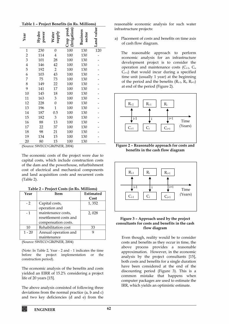
ENGINEER 62

Table 1 – Project Benefits (in Rs. Millions) Ye

ar

Hyd

ro

pow

er

Wat

er

supp

ly

Cro

p p

rod.

(I

rrig

atio

n)

Busi

ness

se

ctor

Land

val

ue

1 230 0 100 130 120 2 114 4 100 130 - 3 101 28 100 130 - 4 146 42 100 130 - 5 192 2 100 130 - 6 103 43 100 130 - 7 75 73 100 130 - 8 149 22 100 130 - 9 141 17 100 130 - 10 145 18 100 130 - 11 163 3 100 130 - 12 228 0 100 130 - 13 196 1 100 130 - 14 187 0.5 100 130 - 15 182 3 100 130 - 16 88 13 100 130 - 17 22 37 100 130 - 18 98 21 100 130 - 19 134 15 100 130 - 20 80 15 100 130 -

(Source: SWECO GRØNER, 2004) The economic costs of the project were due to capital costs, which include construction costs of the dam and the powerhouse, refurbishment cost of electrical and mechanical components and land acquisition costs and recurrent costs (Table 2).

Table 2 – Project Costs (in Rs. Millions) Year Item Estimated

Cost - 2

Capital costs, operation and maintenance costs, resettlement costs and compensation costs.

1, 352

- 1 2, 028

10 Rehabilitation cost 33 1 - 20 Annual operation and

maintenance 9

(Source: SWECO GRØNER, 2004) (Note: In Table 2, Year - 2 and - 1 indicates the time before the project implementation or the construction period). The economic analysis of the benefits and costs yielded an EIRR of 15.2% considering a project life of 20 years [15]. The above analysis consisted of following three deviations from the normal practice (a, b and c) and two key deficiencies (d and e) from the

reasonable economic analysis for such water infrastructure projects: a) Placement of costs and benefits on time axis

of cash flow diagram. The reasonable approach to perform

economic analysis for an infrastructure development project is to consider the operation and maintenance costs (Ci-1, Ci, Ci+1) that would incur during a specified time unit (usually 1 year) at the beginning of the period and the benefits (Ri-1, Ri, Ri+1) at end of the period (Figure 2).

Figure 2 – Reasonable approach for costs and

benefits in the cash flow diagram

Figure 3 – Approach used by the project consultants for costs and benefits in the cash

flow diagram Even though, reality would be to consider costs and benefits as they occur in time, the above process provides a reasonable approximation. However, in the economic analysis by the project consultants [15], both costs and benefits for a single duration have been considered at the end of the discounting period (Figure 3). This is a common mistake that happens when computer packages are used to estimate the IRR, which yields an optimistic estimate.

i-1 i i+1 Time

(Years)

Ri-1 Ri Ri+1

Ci-1 Ci Ci+1

i-1 i i+1 Time

(Years)

Ri-2 Ri-1 Ri

Ci-1 Ci Ci+1

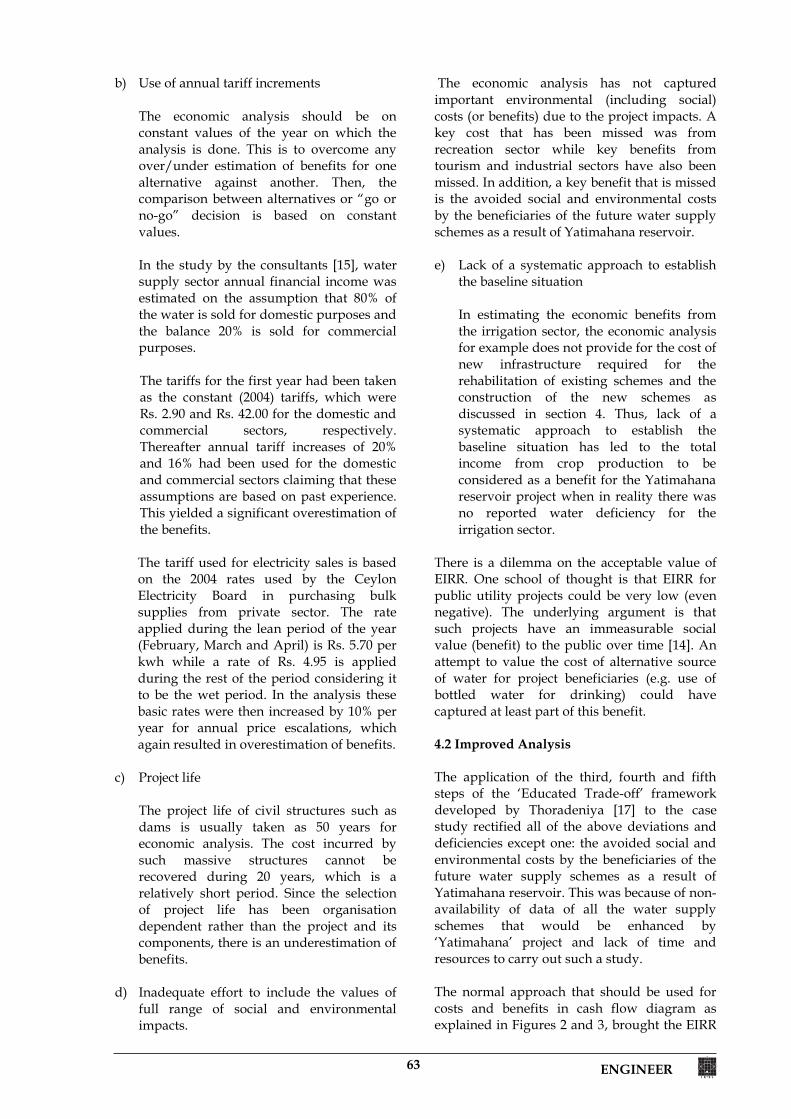
63 ENGINEER

b) Use of annual tariff increments

The economic analysis should be on constant values of the year on which the analysis is done. This is to overcome any over/under estimation of benefits for one alternative against another. Then, the comparison between alternatives or “go or no-go” decision is based on constant values. In the study by the consultants [15], water supply sector annual financial income was estimated on the assumption that 80% of the water is sold for domestic purposes and the balance 20% is sold for commercial purposes.

The tariffs for the first year had been taken as the constant (2004) tariffs, which were Rs. 2.90 and Rs. 42.00 for the domestic and commercial sectors, respectively. Thereafter annual tariff increases of 20% and 16% had been used for the domestic and commercial sectors claiming that these assumptions are based on past experience. This yielded a significant overestimation of the benefits.

The tariff used for electricity sales is based on the 2004 rates used by the Ceylon Electricity Board in purchasing bulk supplies from private sector. The rate applied during the lean period of the year (February, March and April) is Rs. 5.70 per kwh while a rate of Rs. 4.95 is applied during the rest of the period considering it to be the wet period. In the analysis these basic rates were then increased by 10% per year for annual price escalations, which again resulted in overestimation of benefits.

c) Project life

The project life of civil structures such as dams is usually taken as 50 years for economic analysis. The cost incurred by such massive structures cannot be recovered during 20 years, which is a relatively short period. Since the selection of project life has been organisation dependent rather than the project and its components, there is an underestimation of benefits.

d) Inadequate effort to include the values of

full range of social and environmental impacts.

The economic analysis has not captured important environmental (including social) costs (or benefits) due to the project impacts. A key cost that has been missed was from recreation sector while key benefits from tourism and industrial sectors have also been missed. In addition, a key benefit that is missed is the avoided social and environmental costs by the beneficiaries of the future water supply schemes as a result of Yatimahana reservoir. e) Lack of a systematic approach to establish

the baseline situation

In estimating the economic benefits from the irrigation sector, the economic analysis for example does not provide for the cost of new infrastructure required for the rehabilitation of existing schemes and the construction of the new schemes as discussed in section 4. Thus, lack of a systematic approach to establish the baseline situation has led to the total income from crop production to be considered as a benefit for the Yatimahana reservoir project when in reality there was no reported water deficiency for the irrigation sector.

There is a dilemma on the acceptable value of EIRR. One school of thought is that EIRR for public utility projects could be very low (even negative). The underlying argument is that such projects have an immeasurable social value (benefit) to the public over time [14]. An attempt to value the cost of alternative source of water for project beneficiaries (e.g. use of bottled water for drinking) could have captured at least part of this benefit. 4.2 Improved Analysis The application of the third, fourth and fifth steps of the ‘Educated Trade-off’ framework developed by Thoradeniya [17] to the case study rectified all of the above deviations and deficiencies except one: the avoided social and environmental costs by the beneficiaries of the future water supply schemes as a result of Yatimahana reservoir. This was because of non-availability of data of all the water supply schemes that would be enhanced by ‘Yatimahana’ project and lack of time and resources to carry out such a study. The normal approach that should be used for costs and benefits in cash flow diagram as explained in Figures 2 and 3, brought the EIRR

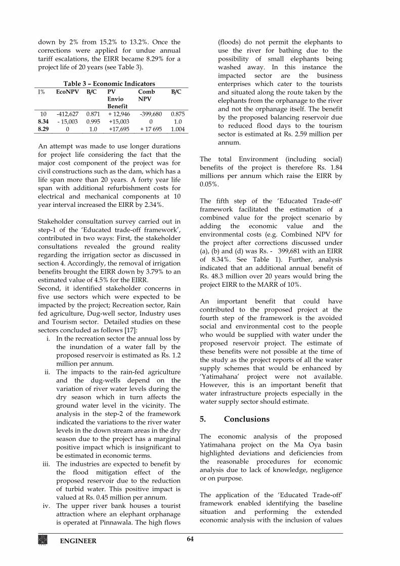
ENGINEER 64

down by 2% from 15.2% to 13.2%. Once the corrections were applied for undue annual tariff escalations, the EIRR became 8.29% for a project life of 20 years (see Table 3).

Table 3 – Economic Indicators I% EcoNPV B/C PV

Envio Benefit

Comb NPV

B/C

10 -412,627 0.871 + 12,946 -399,680 0.875 8.34 - 15,003 0.995 +15,003 0 1.0 8.29 0 1.0 +17,695 + 17 695 1.004 An attempt was made to use longer durations for project life considering the fact that the major cost component of the project was for civil constructions such as the dam, which has a life span more than 20 years. A forty year life span with additional refurbishment costs for electrical and mechanical components at 10 year interval increased the EIRR by 2.34%. Stakeholder consultation survey carried out in step-1 of the ‘Educated trade-off framework’, contributed in two ways: First, the stakeholder consultations revealed the ground reality regarding the irrigation sector as discussed in section 4. Accordingly, the removal of irrigation benefits brought the EIRR down by 3.79% to an estimated value of 4.5% for the EIRR. Second, it identified stakeholder concerns in five use sectors which were expected to be impacted by the project; Recreation sector, Rain fed agriculture, Dug-well sector, Industry uses and Tourism sector. Detailed studies on these sectors concluded as follows [17]:

i. In the recreation sector the annual loss by the inundation of a water fall by the proposed reservoir is estimated as Rs. 1.2 million per annum.

ii. The impacts to the rain-fed agriculture and the dug-wells depend on the variation of river water levels during the dry season which in turn affects the ground water level in the vicinity. The analysis in the step-2 of the framework indicated the variations to the river water levels in the down stream areas in the dry season due to the project has a marginal positive impact which is insignificant to be estimated in economic terms.

iii. The industries are expected to benefit by the flood mitigation effect of the proposed reservoir due to the reduction of turbid water. This positive impact is valued at Rs. 0.45 million per annum.

iv. The upper river bank houses a tourist attraction where an elephant orphanage is operated at Pinnawala. The high flows

(floods) do not permit the elephants to use the river for bathing due to the possibility of small elephants being washed away. In this instance the impacted sector are the business enterprises which cater to the tourists and situated along the route taken by the elephants from the orphanage to the river and not the orphanage itself. The benefit by the proposed balancing reservoir due to reduced flood days to the tourism sector is estimated at Rs. 2.59 million per annum.

The total Environment (including social) benefits of the project is therefore Rs. 1.84 millions per annum which raise the EIRR by 0.05%. The fifth step of the ‘Educated Trade-off’ framework facilitated the estimation of a combined value for the project scenario by adding the economic value and the environmental costs (e.g. Combined NPV for the project after corrections discussed under (a), (b) and (d) was Rs. - 399,681 with an EIRR of 8.34%. See Table 1). Further, analysis indicated that an additional annual benefit of Rs. 48.3 million over 20 years would bring the project EIRR to the MARR of 10%. An important benefit that could have contributed to the proposed project at the fourth step of the framework is the avoided social and environmental cost to the people who would be supplied with water under the proposed reservoir project. The estimate of these benefits were not possible at the time of the study as the project reports of all the water supply schemes that would be enhanced by ‘Yatimahana’ project were not available. However, this is an important benefit that water infrastructure projects especially in the water supply sector should estimate. 5. Conclusions The economic analysis of the proposed Yatimahana project on the Ma Oya basin highlighted deviations and deficiencies from the reasonable procedures for economic analysis due to lack of knowledge, negligence or on purpose. The application of the ‘Educated Trade-off’ framework enabled identifying the baseline situation and performing the extended economic analysis with the inclusion of values

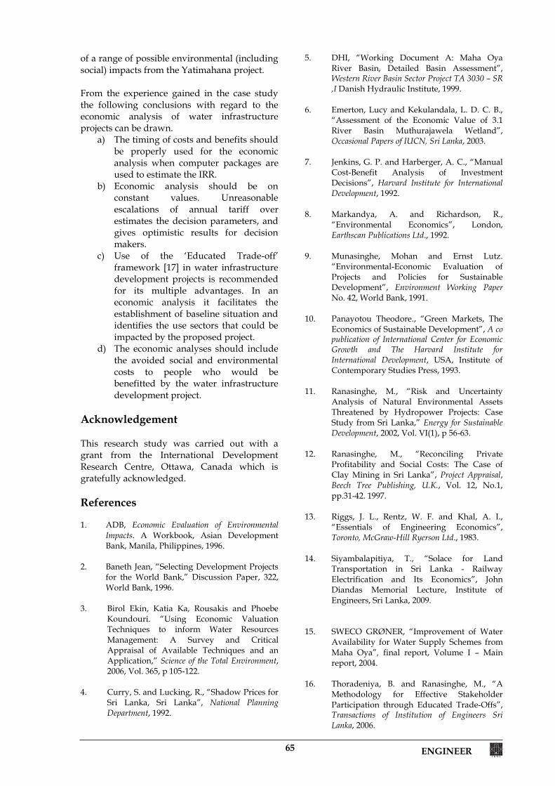
65 ENGINEER

of a range of possible environmental (including social) impacts from the Yatimahana project. From the experience gained in the case study the following conclusions with regard to the economic analysis of water infrastructure projects can be drawn.

a) The timing of costs and benefits should be properly used for the economic analysis when computer packages are used to estimate the IRR.

b) Economic analysis should be on constant values. Unreasonable escalations of annual tariff over estimates the decision parameters, and gives optimistic results for decision makers.

c) Use of the ‘Educated Trade-off’ framework [17] in water infrastructure development projects is recommended for its multiple advantages. In an economic analysis it facilitates the establishment of baseline situation and identifies the use sectors that could be impacted by the proposed project.

d) The economic analyses should include the avoided social and environmental costs to people who would be benefitted by the water infrastructure development project.

Acknowledgement This research study was carried out with a grant from the International Development Research Centre, Ottawa, Canada which is gratefully acknowledged. References 1. ADB, Economic Evaluation of Environmental

Impacts. A Workbook, Asian Development Bank, Manila, Philippines, 1996.

2. Baneth Jean, “Selecting Development Projects

for the World Bank,” Discussion Paper, 322, World Bank, 1996.

3. Birol Ekin, Katia Ka, Rousakis and Phoebe Koundouri. “Using Economic Valuation Techniques to inform Water Resources Management: A Survey and Critical Appraisal of Available Techniques and an Application,” Science of the Total Environment, 2006, Vol. 365, p 105-122.

4. Curry, S. and Lucking, R., “Shadow Prices for

Sri Lanka, Sri Lanka”, National Planning Department, 1992.

5. DHI, “Working Document A: Maha Oya River Basin, Detailed Basin Assessment”, Western River Basin Sector Project TA 3030 – SR ,I Danish Hydraulic Institute, 1999.

6. Emerton, Lucy and Kekulandala, L. D. C. B.,

“Assessment of the Economic Value of 3.1 River Basin Muthurajawela Wetland”, Occasional Papers of IUCN, Sri Lanka, 2003.

7. Jenkins, G. P. and Harberger, A. C., “Manual

Cost-Benefit Analysis of Investment Decisions”, Harvard Institute for International Development, 1992.

8. Markandya, A. and Richardson, R.,

“Environmental Economics”, London, Earthscan Publications Ltd., 1992.

9. Munasinghe, Mohan and Ernst Lutz.

“Environmental-Economic Evaluation of Projects and Policies for Sustainable Development”, Environment Working Paper No. 42, World Bank, 1991.

10. Panayotou Theodore., “Green Markets, The

Economics of Sustainable Development”, A co publication of International Center for Economic Growth and The Harvard Institute for International Development, USA, Institute of Contemporary Studies Press, 1993.

11. Ranasinghe, M., “Risk and Uncertainty

Analysis of Natural Environmental Assets Threatened by Hydropower Projects: Case Study from Sri Lanka,” Energy for Sustainable Development, 2002, Vol. VI(1), p 56-63.

12. Ranasinghe, M., “Reconciling Private

Profitability and Social Costs: The Case of Clay Mining in Sri Lanka”, Project Appraisal, Beech Tree Publishing, U.K., Vol. 12, No.1, pp.31-42. 1997.

13. Riggs, J. L., Rentz, W. F. and Khal, A. I.,

“Essentials of Engineering Economics”, Toronto, McGraw-Hill Ryerson Ltd., 1983.

14. Siyambalapitiya, T., “Solace for Land

Transportation in Sri Lanka - Railway Electrification and Its Economics”, John Diandas Memorial Lecture, Institute of Engineers, Sri Lanka, 2009.

15. SWECO GRØNER, “Improvement of Water Availability for Water Supply Schemes from Maha Oya”, final report, Volume I – Main report, 2004.

16. Thoradeniya, B. and Ranasinghe, M., “A Methodology for Effective Stakeholder Participation through Educated Trade-Offs”, Transactions of Institution of Engineers Sri Lanka, 2006.

ENGINEER 66

17. Thoradeniya, B, “Stakeholder Involvement in

the Decision Making for Development Projects Using ‘Educated Trade-Offs’”, Ph D thesis, 2009.

18. Thoradeniya, B. and Ranasinghe, M., Key

note address, International Conference in Building Education and Research, Kandalama, Sri Lanka., 10-15 February, 2008.

19. Thoradeniya, W. B. M., “Evaluation Report

on the longest serving Area Water Partnership in Sri Lanka”, Lanka Jalani, Colombo, 2005.

20. Vedula, S. and Mujumdar, P. P., “Water Resources Systems, Modeling Techniques and Analysis”, New Delhi, Tata McGraw-Hill Publishing Company Limited, 2005.