vol. 3, no. 2, 1999 pdf - journal of applied measurement
TRANSCRIPT

EDITOR
Richard M Smith Rehabilitation Foundation Inc
ASSOCIATE EDITORS
Benjamin D Wright University of Chicago Richard F Harvey RMClMarianjoy Rehabilitation Hospital amp Clinics Carl V Granger State University of Buffalo (SUNY)
HEALTH SCIENCES EDITORIAL BOARD
David Cella Evanston Northwestern Healthcare William Fisher Jr Louisiana State University Medical Center Anne Fisher Colorado State University Gunnar Grimby University of Goteborg Perry N Halkitis New York University Allen Heinemann Rehabilitation Institute of Chicago Mark Johnston Kessler Institute for Rehabilitation David McArthur UCLA School of Public Health Robert Rondinelli University of Kansas Medical Center Tom Rudy University of Pittsburgh Mary Segal Moss Rehabilitation Alan Tennant University of Leeds Luigi Tesio Foundazione Salvatore Maugeri Pavia Craig Velozo University of Illinois Chicago
EDUCATIONALIPSYCHOLOGICAL EDITORIAL BOARD
David Andrich Murdoch University Trevor Bond James Cook University Ayres DCosta Ohio State University Barbara Dodd University of Texas Austin George Engelhard Jr Emory University
Tom Haladyna Arizona State University West Robert Hess Arizona State University West William Koch University of Texas Austin Joanne Lenke Psychological Corporation J Michael Linacre MESA Press Geofferey Masters Australian Council on Educational Research Carol Myford Educational Testing Service Nambury Raju Illinois Institute of Technology Randall E Schumacker University of North Texas Mark Wilson University of California Berkeley
JOURNAL OF OUTCOME MEASUREMENTreg
1999Volume 3 Numler 2
Articles
Investigating Rating Scale Category Utility 103 John M Linacre
Using IRT Variable Maps to Enrich Understanding of Rehabilitation Data 123
Wendy Coster Larry Ludlow and Marisa Mancini
Measuring Pretest-Posttest Change with a Rasch Rating Scale Model 134
Edward W Wolfe and Chris W T Chiu
Grades of Severity and the Validation of an Atopic Dermatitis Assessment Measure (ADAM) 162
Denise P Charman and George A Varigos
Parameter Recovery for the Rating Scale Model Using PARSCALE 176
Guy A French and Barbara G Dodd
IndexingAbstracting Services JOM is currently indexed in the Current Index to Journals in Education (ERIC) Index Medicus and MEDLINE The paper used in this publication meets the requirements of ANSIINISO Z39 48-1992 (Permanence of Paper)
JOURNAL OF OUTCOME MEASUREMENTreg 3(2) 103-122
Copyright 1999 Rehabilitation Foundation Inc
Investigating Rating Scale Category Utility
John M Linacre University of Chicago
Eight guidelines are suggested to aid the analyst in investigating whether rating scales categories are cooperating to produce observations on which valid measurement can be based These guidelines are presented within the context of Rasch analysis They address features of rating-scale-based data such as category frequency ordering rating-to-measure inferential coherence and the quality of the scale from measurement and statistical perspectives The manner in which the guidelines prompt recategorization or reconceptualization of the rating scale is indicated Utilization of the guidelines is illustrated through their application to two published data sets
Requests for reprints should be sent to John M Linacre MESA Psychometric Laborashytory University of Chicago 5835 S Kimbark Avenue Chicago IL 60637 e-mail mesauchicagoedu
104 LINACRE
Introduction
A productive early step in the analysis of questionnaire and survey data is an investigation into the functioning of rating scale categories Though polytomous observations can be used to implement multidimensional sysshytems (Rasch and Stene 1967 Fischer 1995) observations on a rating scale are generally intended to capture degrees of just one attribute ratshying scales use descriptive terms relating to the factor in question (Stanley and Hopkins 1972 p 290) This factor is also known as the latent trait or variable The rating scale categorizations presented to respondents are intended to elicit from those respondents unambiguous ordinal indishycations of the locations of those respondents along such variables of inshyterest Sometimes however respondents fail to react to a rating scale in the manner the test constructor intended (Roberts 1994)
Investigation of the choice and functioning of rating scale categoshyries has a long history in social science Rating scale categorizations should be well-defined mutually exclusive univocal and exhaustive (Guilford 1965) An early finding by Rensis Likert (1932) is that differshyential category weighting schemes (beyond ordinal numbering) are unshyproductive He proposes the well-known five category agreement scale Nunnally (1967) favors eliminating the neutral category in bi-polar scales such as Likerts and presenting respondents an even number of categoshyries Nunnally (1967 p 521) summarizing Guilford (1954) also reports that in terms of psychometric theory the advantage is always with using more rather than fewer steps Nevertheless he also states that the only exception would occur in instances where a large number of steps conshyfused subjects or irritated them More recently Stone and Wright (1994) demonstrate that in a survey of perceived fear combining five ordered categories into three in the data increases the test reliability for their sample Zhu et al (1997) report similar findings for a self-efficacy scale
Since the analyst is always uncertain ofthe exact manner in which a particular rating scale will be used by a particular sample investigation of the functioning of the rating scale is always merited In cooperation with many other statistical and psycho-linguistic tools Rasch analysis provides an effective framework within which to verify and perhaps imshyprove the functioning of rating scale categorization
Rasch Measurement Models for Rating Scales
A basic Rasch model for constructing measures from observations
INVESTIGATING RATING SCALE CATEGORY UTILITY 105
on an ordinal rating scale is (Andrich 1978)
(1)log ( Pnik Pni(k-I) ) = Bn - Di - Fk
where Pnik is the probability that person n on encountering item i would be observed in category k Pni(k-I) is the probability that the observation would be in category k-l Bn is the ability (attitude etc) of person n Di is the difficulty of item i Fk is the impediment to being observed in category k relative to catshyegory k-l ie the kth step calibration where the categories are numshybered Om
This and similar models not only meet the necessary and sufficient conditions for the construction of linear measures from ordinal observashytions (Fischer 1995) but also provide the basis for investigation of the operation of the rating scale itself The Rasch parameters reflecting the structure of the rating scale the step calibrations are also known as threshshyolds (Andrich 1978)
The prototypical Likert scale has five categories (Strongly Disagree Disagree Undecided Agree Strongly Agree) These are printed equally spaced and equally sized on the response form (see Figure 1) The intenshytion is to convey to the respondent that these categories are of equal imshyportance and require equal attention They form a clear progression and they exhaust the underlying variable
IDisagree I I Und~ided I 3 Figure 1 Prototypical Likert scale as presented to the respondent
From a measurement perspective the rating scale has a different appearance (Figure 2) The rating categories still form a progression and exhaust the underlying variable The variable however is conceptually infinitely long so that the two extreme categories are also infinitely wide However strongly a particular respondent agrees we can always posit one who agrees yet more strongly ie who exhibits more of the latent variable The size of the intermediate categories depends on how they are perceived and used by the respondents Changing the description of the middle category from Undecided to Unsure or Dont Know or
6 08 Ol Ql
C 07 u +shy
o 06 s o ~ 05 gt shyQl ] 04middotmiddotmiddot o 0 03middotmiddot gtshy
+shy
6 02middotmiddotmiddot o
0
~ 01 a
Strongly Disagree
106 LINACRE
Dont Care will change its meaning psycho-linguistically and so the amount of the underlying variable it represents its size as depicted in Figure 2 In view of the general proclivity of respondents towards social conformity agreeability or mere lethargy the agree option is usually more attractive than the disagree one Hence the agree category tends to represent a wider range of the underlying variable
Strongly Disagree
Agree Strongly Agree
- - Latent Variable - shy
Figure 2 Prototypical Likert scale from a measurement perspective
Empirically the observations manifest a stochastic element The analysts expectation is that the probability of observing each category is greatest where that category is modeled to occur on the latent variable but there is always some possibility of observing any category at any point on the continuum Figure 3 shows probability curves for each category in accordance with Rasch model specifications (Wright and Masters 1982 p81)
09 --~-___
gt- Agree
O+-~~--~~r---r-~~~~~~-~~=-~ -5 -4 -3 -2 -1 0 2 3 4 5
Latent Variable
Figure 3 Category probability curves for 5 category Likert scale
INVESTIGATING RATING SCALE CATEGORY UTILITY 107
In practice data do not conform exactly to Rasch model specificashytions or those of any other ideal model For problem solving purposes we do not require an exact but only an approximate resemblance between theoshyretical results and experimental ones (Laudan 1977 p 224) For analytishycal purposes the challenge then becomes to ascertain that the rating scale observations conform reasonably closely to a specified model such as that graphically depicted in Figure 3 When such conformity is lacking the analyst requires notification as to the nature of the failure in the data and guidance as to how to remedy that failure in these or future data
How the variable is divided into categories affects the reliability of a test Mathematically it can be proven that when the data fit the Rasch model there is one best categorization to which all others are inferior (Jansen and Roskam 1984) Since this best categorization may not be observed in the raw data guidelines have been suggested for combining categories in order to improve overall measure quality (Wright and Linacre 1992) Fit statistics step calibrations and other indicators have also been suggested as diagnostic aids (Linacre 1995 Andrich 1996 Lopez 1996)
The Heuristic Analysis of Rating Scale Observations
At this point we set aside the linguistic aspects of category definitions (Lopez 1996) taking for granted that the categories implement a clearly deshyfined substantively relevant conceptually exhaustive ordered sequence We consider solely the numerical information that indicates to what extent the data produce coherent raw scores ie raw scores that support the construcshytion of Rasch measures The description of the characteristics of an ideal rating scale presented above suggests an explicit procedure for verifying useful functioning and diagnosing malfunctioning
) Table 1
Analysis ofGuilfords (1954) rating scale
Category Average Expected OUTFIT Step CategoryLabel Count Measure Measure MnSq Calibration Name
1 4 4 - 85 -73 8 - lowest 2 4 4 -11 - 57 26 - 63 3 25 24 - 36 - 40 9 -231 4 8 8 - 43 - 22 5 84 5 31 30 - 04 -03 8 -148 middle 6 6 6 - 46 16 41 1 71 7 21 20 45 34 6 -1 01 8 3 3 74 49 5 235 9 3 3 76 61 7 53 highest
108 LINACRE
gtshy~ 09 Cgt
-6 08 u 0 07 c ~ 06middotmiddot C gta 05 In
lt304 o -~03
g 02 c ott 01
-2 -1 2 Latent Variable
Figure 4 Rasch model category probability curves for Guilfords (1954) scale
Table 2
Analysis ofLFS rating scale data
Category Average Expeoted OUTFIT Step Coherenoe Soore-to-Meaaure Label Count Measure Measure IInSq Calibration II-gtC C-gtII ----Zone---shy
0 578 -87 -LOS 119 NONE 65115 4211 -- -118 1 620 15 55 69 - 85 54115 71 -118 118 2 852 223 215 146 85 85115 781s 118 +shy
Consider the Ratings of Creativity (Guilford 1954) also discussed from a different perspective in Linacre (1989) Table 1 contains results from an analysis by Facets (Linacre 1989) The model category characshyteristic curves are shown in Figure 4 These will be contrasted with the Liking for Science (LFS) ratings reported in Wright and Masters (1982) Table 2 contains results from an analysis by BIGSTEPS (Wright and Linacre 1991) The model category characteristic curves for the LFS data are shown in Figure 5
Guideline 1 At least 10 observations of each category
Each step calibration Fk is estimated from the log-ratio of the freshyquency of its adjacent categories When category frequency is low then the step calibration is imprecisely estimated and more seriously potenshytially unstable The inclusion or exclusion of one observation can noticeshyably change the estimated scale structure
c
INVESTIGATING RATING SCALE CATEGORY UTILITY 109
gtshy~ 09 Cl CDC 08 u Dislike Like 0 07
206 Neuttal o gt ~ 05 ()
c5 04 o ~ 03
g 02 a oct 01
Omiddotmiddot~ww=middotmiddotmiddot=middot~c-~middot-~- Y__-+__ =~====~ -3 -2 -1 o 2 3
Latent Variable
Figure 5 Model probability characteristic curves for LFS rating scale
For instance omitting one often observations changes the step calishybration by more than 1 logits (more than 2 logits for one of 5) If each item is defined to have its own rating scale ie under partial credit conshyditions this would also change the estimated item difficulty by 1Im when there are m+1 categories and so m steps For many data sets this value would exceed the model standard error of the estimated item difficulty based on 100 observations Consequently the paradox can arise that a sample large enough to provide stable item difficulty estimates for less statistically informative dichotomous items (Linacre 1994) may not be sufficiently large for more informative polytomous items
Categories which are not observed in the current dataset require speshycial attention First are these structural or incidental zeros Structural zeros correspond to categories of the rating scale which will never be observed They may be an artifact of the numbering of the observed catshyegories eg categories 2 and 4 cannot be observed when there are only three scale categories and these are numbered 1 3 and 5 Or structural zeros occur for categories whose requirements are impossible to fulfil eg in the 17th Century it was conventional to assign the top category to God-level performance For these structural zeros the catshy
110 LINACRE
egories are simply omitted and the remaining categories renumbered seshyquentially to represent the only observable qualitative levels of perforshymance
Incidental zeroes are categories that have not been observed in this particular data set Thus all categories of a 5 category scale cannot be seen in just three observations There are several strategies that avoid modifying the data i) treat those incidental zeroes as structural for this analysis renumbering the categories without them ii) impose a scale strucshyture (by anchoring thresholds) that includes these categories iii) use a mathematical device (Wilson 1991) to keep intermediate zero categories in the analysis
In the Guilford example (Table 1) category frequency counts as low as 3 are observed When further relevant data cannot be easily obtained one remedy is to combine adjacent categories to obtain a robust structure of high frequency categories Another remedy is to omit observations in low frequency categories that may not be indicative of the main thrust of the latent variable Such off-dimension categories may be labeled dont know or not applicable The frequency count column by itself sugshygests that the rarely observed categories 124689 be combined with adjacent categories or their data be omitted The remaining categories would be renumbered sequentially and then the data reanalyzed
In the LFS example (Table 2) all category frequency counts are large indicating that locally stable estimates of the rating scale structure can be produced
Guideline 2 Regular observation distribution
Irregularity in observation frequency across categories may signal aberrant category usage A uniform distribution of observations across categories is optimal for step calibration Other substantively meaningful distributions include unimodal distributions peaking in central or extreme categories and bimodal distributions peaking in extreme categories Probshylematic are distributions of roller-coaster form and long tails of relashytively infrequently used categories On the other hand when investigating highly skewed phenomena eg criminal behavior or creative genius the long tails of the observation distribution may capture the very informashytion that is the goal of the investigation
A consideration when combining or omitting categories is that the rating scale may have a substantive pivot-point the point at which the subshy
INVESTIGATING RATING SCALE CATEGORY UTILITY III
stantive meaning of the ratings is dichotomized For instance when using a Likert scale to ask about socially-acceptable propositions such as Crime should be punished the pivot point could be between Strongly Agree and Agree For negatively worded propositions such as Politicians are dishonest the pivot could be between Disagree and Neutral
In Table 1 the frequency distribution is tri-modal with peaks at 35 and 7 perhaps indicating that the judges are being asked to apply a 9 category scale to performances that they can only discriminate into three levels Again remedies include combining adjacent categories or omitshyting observations in categories such as Other whose measurement imshyplications are dubious A regular frequency distribution in Table 1 could be obtained by combining categories 12 and 3 totaling 33 also 4 and 5 totaling 39 and then 6 7 8 and 9 totaling 33
In Table 2 the frequency distribution is unimodal and shows reasshysuringly smooth increases from approximately 380 to 620 (a jump of 240) and then from 620 to 850 (a jump of 230)
Guideline 3 Average measures advance monotonically with category
Equation (1) specifies a Rasch measurement model This is concepshytualized to generate data in the following fashion
B - D - F ==gt X (2)n 1 k nl
where Xni is the rating observed when person n encountered item i Fk is the set of step calibrations for all categories 0 m and other parameters have the meanings assigned in (1)
Within anyone item or group of items modeled to have the same rating scale structure the Fk are constant across observations and may be ignored at this point It is the combination of B nand Di (or their equivashylent in any other Rasch model) that is crucial in producing and then diagshynosing the empirical observation Xni It is essential to our comprehension of the rating scale that in general higher measure combinations (Bn - D) produce observations in higher categories and vice-versa Accordingly a diagnostic indicator is the average of the measures (B - D) across all
n I
observations in each category
These average measures are an empirical indicator of the context in which the category is used In general observations in higher categories must be produced by higher measures (or else we dont know what a higher
112 LINACRE
measure implies) This means that the average measures by category for each empirical set of observations must advance monotonically up the ratshying scale Otherwise the meaning of the rating scale is uncertain for that data set and consequently any derived measures are of doubtful utility
In Table 1 failures of average measures to demonstrate monotonicity are flagged by In particular the average measure corresponding to the 6 observations in category 6 is -46 noticeably less than the -04 for the 31 observations in category 5 Empirically category 6 does not manifest higher performance levels than category 5 An immediate remedy is to combine non-advancing (or barely advancing) categories with those below them and so obtain a clearly monotonic structure The average measure column of Table 2 by itself suggests that categories 2 3 and 4 be combined and also categories 5 6 and 7 Categories 18 and 9 are already monotonic
In Table 2 the average measures increase monotonically with rating scale category from -87 to 1310gits (a jump of 10) and then from 13 to 223 (a jump of 22) This advance is empirical confirmation of our intenshytion that higher rating scale categories indicate more of the latent varishyable The advances across categories however are uneven This may be symptomatic of problems with the use of the rating scale or may merely reflect the item and sample distributions
The Expected Measure columns in Tables 1 and 2 contain the valshyues that the model predicts would appear in the Average Measure colshyumns were the data to fit the model In Table 1 these values are diagnostically useful For category 1 the observed and expected values -85 and -73 are close For category 2 however the observed value ofshy11 is 4610gits higher than the expected value of 57 and also higher than the expected value for category 4 Category 6 is yet more aberrant with an observed average measure less than the expected average measure for category 3 The observations in categories 2 and 6 are so contradictory to the intended use of the rating scale that even on this slim evidence it may be advisable to remove them from this data set
In Table 2 the observed average measures appear reasonably close to their expected values
Guideline 4 OUTFIT mean-squares less than 20
The Rasch model is a stochastic model It specifies that a reasonably uniform level of randomness must exist throughout the data Areas within the data with too little randomness ie where the data are too predictable
INVESTIGATING RATING SCALE CATEGORY UTILITY 113
tend to expand the measurement system making performances appear more d~fferent Areas with excessive randomness tend to collapse the measureshyment system making performances appear more similar Ofthese two flaws excessive randomness ndise is the more immediate threat to the meashysurement system
For the Rasch model mean-square fit statistics have been defined such that the model-specified uniform value of randomness is indicated by 10 (Wright and Panchapakesan 1969) Simulation studies indicate that values above 15 ie with more than 50 unexplained randomness are problemshyatic (Smith 1996) Values greater than 20 suggest that there is more unexshyplained noise than explained noise so indicating there is more misinformation than information in the observations For the outlier-sensitive OUTFIT meanshysquare this misinformation may be confined to a few substantively explainshyable and easily remediable observations Nevertheless large mean-squares do indicate that segments of the data may not support useful measurement
For rating scales a high mean-square associated with a particular category indicates that the category has been used in unexpected conshytexts Unexpected use of an extreme category is more likely to produce a high mean-square than unexpected use of a central category In fact censhytral categories often exhibit over-predictability especially in situations where respondents are cautious or apathetic
In Table 1 category 6 has an excessively high mean-square of 41 It has more than three times as much noise as explained stochasticity From the standpoint of the Rasch model these 6 observations were highly unpredictable Inspection of the data however reveals that only one of the three raters used this category and that it was used in an idiosyncratic manner Exploratory solutions to the misfit problem could be to omit individual observations combine categories or drop categories entirely Category 2 with only 4 observations also has a problematic mean-square of 21 One solution based on mean-square information alone would be to omit all observations in categories 2 and 6 from the analysis
In Table 2 central category 1 with mean-square 69 is showing some over-predictability In the data one respondent choose this category in reshysponses to all 25 items suggesting that eliminating that particular respondents data would improve measurement without losing information Extreme category 2 with mean-square 146 is somewhat noisy This high value is cause by a mere 6 observations Inspection of these ratings for data entry errors and other idiosyncracies is indicated
114 LINACRE
Guideline 5 Step calibrations advance
The previous guidelines have all considered aspects of the current samples use ofthe rating scale This guideline concerns the scales infershyential value An essential conceptual feature of rating scale design is that increasing amounts of the underlying variable in a respondent correspond to a progression through the sequentially categories of the rating scale (Andrich 1996) Thus as measures increase or as individuals with increshymentally higher measures are observed each category of the scale in tum is designed to be most likely to be chosen This intention corresponds to probability characteristic curves like those in Figure 3 in which each category in tum is the most probable ie modal These probability curves look like a range of hills The extreme categories always approach a probability of 10 asymptotically because the model specifies that responshydents with infinitely high (or low) measures must be observed in the highshyest (or lowest) categories regardless as to how those categories are defined substantively or are used by the current sample
The realization of this requirement for inferential interpretability of the rating scale is that the Rasch step calibrations Fk advance monotonishycally with the categories Failure of these parameters to advance monotonishycally is referred to as step disordering Step disordering does not imply that the substantive definitions of the categories are disordered only that their step calibrations are Disordering reflects the low probability of obshyservance ofcertain categories because of the manner in which those categoshyries are used in the rating process This degrades the interpretability of the resulting measures Step disordering can indicate that a category represents too narrow a segment of the latent variable or a concept that is poorly deshyfined in the minds of the respondents
Disordering of step calibrations often occurs when the frequencies of category usage follow an irregular pattern The most influential comshyponents in the estimation of the step calibrations are the log-ratio of the frequency of adjacent categories and the average measures of the responshydents choosing each category Thus
Fk log (TkTk) - Bk + Bk_1 (3)
where
Tk is the observed frequency of category k Tk-I is the observed frequency of category k-J Bk is the average measure of respondents choosing category k and Bk_1 is the average measure of those choosing category k-J
INVESTIGATING RATING SCALE CATEGORY UTILITY 115
It can be seen that step-disordering may result when a higher catshyegory is relatively rarely observed or a lower category is chosen by reshyspondents with higher measures
In Table 1 disordered step calibrations are indicated with The step calibrations correspond to the intersections in the probability curve plot Figshyure 4 The step calibration from category 2 to category 3 F3 is -23110gits In Figure 4 this is the point where the probability curves for categories 2 and 3 cross at the left side of the plot It can be seen that category 2 is never modal ie at no point on the variable is category 2 ever the most likely category to be observed The peak of category 2s curve is submerged and it does not apshypear as a distinct hill Figure 4 suggests that a distinct range of hills and so strict ordering of the step calibrations would occur if categories 2 and 3 were combined and also 4 5 and 6 and finally 7 and 8 Since the extreme categoshyries 1 and 9 are always modal it is not clear from this plot whether it would be advantageous to combine one or both of them with a neighboring more central category
In Table 2 the step calibrations -85 and +85 are ordered The corresponding probability curves in Figure 5 exhibit the desired appearshyance of a range of hills
shyGuideline 6 Ratings imply measures and measures imply ratings
In clinical settings action is often based on one observation Conshysequently it is vital that in general a single observation imply an equivashylent underlying measure Similarly from an underlying measure is inferred what behavior can be expected and so in general what rating would be observed on a single item The expected item score ogive the model item characteristic curve (ICC) depicts the relationship between measures and average expected ratings
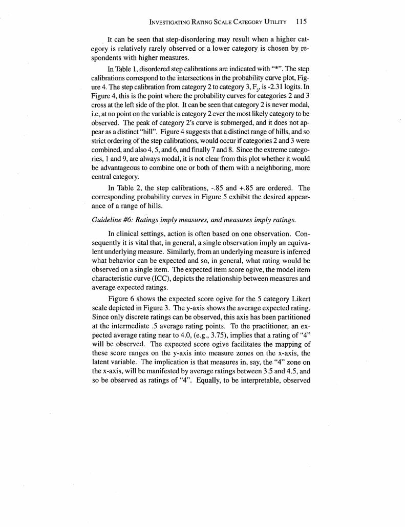
Figure 6 shows the expected score ogive for the 5 category Likert scale depicted in Figure 3 The y-axis shows the average expected rating Since only discrete ratings can be observed this axis has been partitioned at the intermediate 5 average rating points To the practitioner an exshypected average rating near to 40 (eg 375) implies that a rating of 4 will be observed The expected score ogive facilitates the mapping of these score ranges on the y-axis into measure zones on the x-axis the latent variable The implication is that measures in say the 4 zone on the x-axis will be manifested by average ratings between 35 and 45 and so be observed as ratings of 4 Equally to be interpretable observed
116 LINACRE
5
en 45 c -0 4 D
~ 35middotmiddotmiddot +shyu (J) 3 D X
W (J) 25 0)
2 2 (J) gt laquo 15
4 Zone 1 ~----middotmiddot~-------~---middot~--~~-----Tmiddotmiddotmiddotmiddotmiddotmiddotmiddotmiddotmiddot-middot------middotmiddotmiddotmiddotmiddot-middotmiddotmiddot--~ -5 -4 -3 -2 -1 0 1 2 3 4 5
Latent Variable Figure 6 Expected score ogive for 5 category Likert scale showing rating-measure zones
ratings of 4 on the y-axis imply respondent measures within the 4 zone of the latent variable
In Table 2 the Coherence columns report on the empirical relationshyship between ratings and measures for the LFS data The computation of Coherence is outlined in Table 3 M-gtC (Measure implies Category ) reshyports what percentage of the ratings expected to be observed in a category (according to the measures) are actually observed to be in that category
The locations of the measure zone boundaries for each category are shown in Table 2 by the Score-to-Measure Zone columns Consider the M-gtC of category O 63 of the ratings that the measures would place in category 0 were observed to be there The inference ofmeasuresshyto-ratings is generally successful The C-gtM (Category implies Measure ) for category 0 is more troublesome Only 42 of the occurrences of category 0 were placed by the measures in category O The inference of ratings-to-measures is generally less successful Nevertheless experishyence with other data sets (not reported here) indicates that 40 is an emshypirically useful level of coherence
INVESTIGATING RATING SCALE CATEGORY UTILITY 117
Table 3
Coherence of Observations
Observed Rating Observed Rating in Category outside Category
Observed Measure ICIZ OCIZ in Zone (Rating in Figure 7) in Figure 7) ( H
Observed Measure ICOZ shyoutside Zone (x in Figure 7)
M- gtC =In Category amp Zone I All in Zone = ICIZ I (lCIZ + OCIZ) 100
C-gtM = In Category amp Zone f All in Category = ICIZ I (ICIZ + ICOZ) 100
Figure 7 shows the Guttman scalogram for the LFS data partitioned by category for categories 0 1 and 2 left to right In each section ratings observed where their measures predict are reported by their rating value 0 1 or 2 Ratings observed outside their expected measure zone are marked by x Ratings expected in the specified category but not observed there are marked by In each partition the percentage of ratings reported by their category numbers to such ratings ands is given by M-gtC The percentage of ratings reported by their category numbers to such ratings and xs is given by C-gtM In the left-hand panel for category 0 the there are about twice as many Os as s so C-gtM coshyherence of 63 is good On the other hand there are more xs than Os so M-gtC coherence of 42 is fragile The inference from measures to ratings for category degis strong but from ratings to measures is less so This suggests that local inference for these data would be more secure were categories degand 1 to be combined
Guideline 7 Step difficulties advance by at least 14 logits
It is helpful to communicate location on a rating scale in terms of categories below the location ie passed and categories above the locashytion ie not yet reached This conceptualizes the rating scale as a set of dichotomous items Under Rasch model conditions a test of m dichotoshymous items is mathematically equivalent to a rating scale of m+1 categoshyries (Huynh 1994) But a rating scale of m+ 1 categories is only equivalent to test of m dichotomous items under specific conditions (Huynh 1996)
2 41 x 34 xx 17 50 45
x
xx
x x xii
x bullbull x 7 x x x xx
16 48 25 59
x xx x
x x
xll11 x 11 x 111 x xii bullbullbull
22x
2x
2 x 18 x xx x 11 39 xx x xlll 23 xxx XXll111 58 x xx x x ll 57 xxxxx 40 x xx xl 11 70 x xxx xx 1 33 x xxx x 111 38 X x xxllll1110 43 xxxx x 111 1 74 x xxxxx x bullbullbullbullbullbullbullbullbullbull SO x x xXI 1I 111111 S4 X xx 1111111 11 xx xxxO 1 11 22 x 1111111111111 x 56 x xxO x 11 1111
3 x 0 xll111111111 51 xxxxO x 11111 83 x x xO xx l11 111
8 x x xxxOO 11 1 bullbull 69 x xxOO x 11111 bullbull 1 71 x x x xx X X x 1 1 111 X X X xOO x 11 bullbullbull111 24 xx xOO xx 1111 bullbullbullbull 11 42 XOO xxx 111 bullbull 111111 31 0 x x 111111111111x 65 x xx x x x11111 111
1 x xx x 00 1111 bullbull 11 1 54 000 x x xll111111 111 66 x x xx 000 1 bullbull11111 28 xx x xOO xx bullbull 1 bullbull III1 x 61 XXOOO xxxl bullbull 111111 67 x x X OO xx 111 1111xx 10 x xOOOO x x1 111111 x 21 bullbull 000 x l111111111111xx 44 x 00000 x xl11 11111 62 xx x xx xOOOOO 73 x x xxx x bullbullbull 00 III I x
4 x xOOO x ll11111111x x 15 27 xx x 66 x xxxxl1111111111111xx xx
x xlll ll1111x x 35 000 bull x xl1111111111111 37 xOOOOO xl 11 1111111 52 xxxxl1111111111111xxxXX 20 x x xxOOOOO 1111 11 82 x xOOOOO x x 11 111111 46 xxxxxxOOOO 1 x 75 xx x x xOOO 1bullbullbull 11 bullbull 1bullbullbull 11x
x
X
x
x
x
X
x
xx
x
xx
x
x xx x
x x
x x
bull X
x
x
x x
x xx
x x
x
x x x
x
xx
x
xxx
x
x xx
118 LINACRE
ITEIIS ITEIIS
26 xxxxxlll111111111111 xxxxx S6 x x 000 bull x 1111111111111 X 55 x x xOO bullbull O x 111111111 1 xx
6 xx xxx 0 xx11111111 bullbull 1x xx 9 xx x x 00 x 11 111111 x x
13 x x xO 00 xl111111 xxx 47 xxx x 0000 x 1111 bullbullbull1111 x 14 xx x xx xx 0000 1111 x 49 x x x xOO bullbullbull xxx11111111111 x x
5 xx x xOOOO bullbull Xll11 11111x x xxx 68 x x x x 00000000 1 11111 X 12 x x xxxx 00 bull 0000 bullbull xl1 11 xx X x SO xx x 000000000000 11 1 x 29 x xx xOOOOOOOO 00 1111 1 x x 72 x xxx xOOOOOOOO bullbullbullbullO 111 11 x xx 53 xx 00000000 bullbullbull0000 11 1111 xxx
Figure 7 Guttman scalograms of LFS data flagging out-of-zone observations wiht x
For practical purposes when all step difficulty advances are larger than 14 logits then a rating scale of m+1 categories can be decomposed
INVESTIGATING RATING SCALE CATEGORY UTILITY 119
in theory into a series of independent dichotomous items Even though such dichotomies may not be empirically meaningful their possibility implies that the rating scale is equivalent to a sub-test of m dichotomies For developmental scales this supports the interpretation that a rating of k implies successful leaping of k hurdles Nevertheless this degree of rating scale refinement is usually not required in order for valid and infershyentially useful measures to be constructed from rating scale observations
The necessary degree of advance in step difficulties lessens as the number of categories increases For a three category scale the advance must be at least 14 logits between step calibrations in order for the scale to be equivalent to two dichotomies For a five category rating scale adshyvances of at least 10 logits between step calibrations are needed in order for that scale to be equivalent to four dichotomies
In Table 2 the step calibrations advance from -85 to +85 logits a distance of 17 This is sufficiently large to consider the LFS scale statisshytically equivalent to a 2-item sub-test with its items about 12logits apart When the two step calibrations are -7 and +7 then the advance is 14 logits (the smallest to meet this guideline) and the equivalent sub-test comprises two items of equal difficulty When the advance is less than 14logits redefining the categories to have wider substantive meaning or combining categories may be indicated
Guideline 8 Step difficulties advance by less than 50 logits
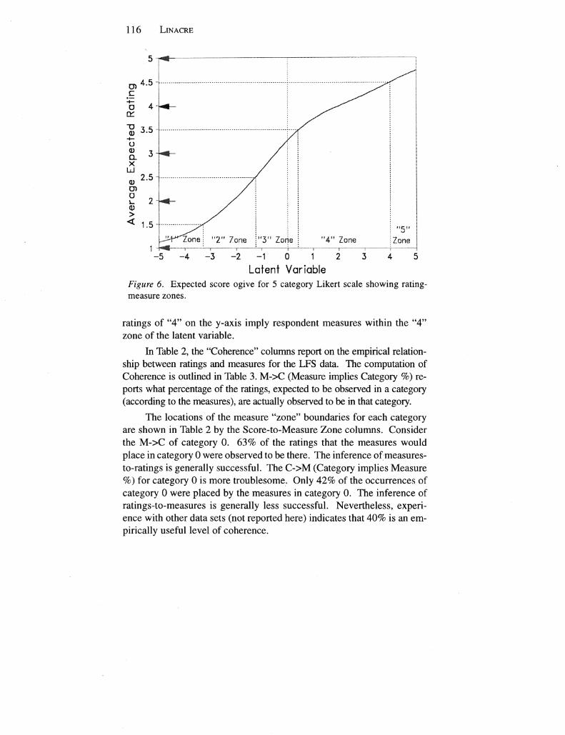
The purpose of adding categories is to probe a wider range of the variable or a narrow range more thoroughly When a category represents a very wide range of performance so that its category boundaries are far apart then a dead zone develops in the middle of the category in which measurement loses its precision This is evidenced statistically by a dip in the information function In practice this can result from Guttmanshystyle (forced consensus) rating procedures or response sets
In Figure 8 the information functions for three category (two step) items are shown When the step calibrations are less than 3 log its apart then the information has one peak mid-way between the step calibrashytions As the step calibrations become farther apart the information funcshytion sags in the center indicating that the scale is providing less information about the respondents apparently targeted best by the scale Now the scale is better at probing respondents at lower and higher decision points than at the center When the distance between step calibrations is more
120 LINACRE
than 5 logits the information provided at the items center is less than half that provided by a simple dichotomy When ratings collected under circumstances which encourage rater consensus are subjected to Rasch analysis wide distances between step calibrations may be observed Disshytances of 30 log its have been seen Such results suggest that the raters using such scales are not locally-independent experts but rather rating machines A reconceptualization of the function of the raters or the use of the rating scale in the measurement process may be needed
045 Step Calibration Advance = 2 logits
04middotmiddot
c 035a-0
03E 6 0 025~ s
0 02 ()
i 015VIshy-+shyc
01 U1
005
0 0=6 =4 =3 =2 -1 0 2 3 4 5
Logit Measure Figure 8 Information functions for a three-category rating scale
In clinical applications discovery of a very wide intermediate category suggests that it may be productive to redefine the category as two narrower categories This redefinition will necessarily move allcategory thresholds but the clinical impact of redefinition of one category on other clearly defined categories is likely to be minor and indeed may be advantageous
Conclusion
Unless the rating scales which form the basis of data collection are functioning effectively any conclusions based on those data will be inseshycure Rasch analysis provides a technique for obtaining insight into how
INVESTIGATING RATING SCALE CATEGORY UTILITY 121
the data cooperate to construct measures The purpose of these guideshylines is to assist the analyst in verifying and improving the functioning of rating scale categories in data that are already extant Not all guidelines are relevant to any particular data analysis The guidelines may even suggest contradictory remedies Nevertheless they provide a useful startshying-point for evaluating the functioning of rating scales
References Andrich D A (1978) A rating formulation for ordered response categories
Psychometrika 43 561-573
Andrich D A (1996) Measurement criteria for choosing among models for graded responses In A von Eye and C C Clogg (Eds) Analysis ofcategorical variables in developmental research Orlando FL Academic Press Chapter 1 3-35
Fischer G H (1995) The derivation of polytomous Rasch models Chapter 16 in G H Fischer and I W Molenaar (Eds) Rasch Models Foundations Reshycent Developments and Applications New York Springer Verlag
Guilford J P (1954) Psychometric Methods 2nd Edn New York McGrawshyHill
Guilford JP (1965) Fundamental Statistics in Psychology and Education 4th Edn New York McGraw-Hill
Huynh H (1994) On equivalence between a partial credit item and a set of independent Rasch binary items Psychometrika 59111-119
Huynh H (1996) Decomposition of a Rasch partial credit item into independent binary and indecomposable trinary items Psychometrika 61(1) 31-39
Jansen PGW and Roskam EE (1984) The polytomous Rasch model and dishychotomization of graded responses p 413-430 in E Degreef and J van Buggenhaut (Eds) Trends in Mathematical Psychology Amsterdam NorthshyHolland
Laudan L (1977) Progress and its Problems Berkeley CA University of Calishyfornia Press
Likert R (1932) A technique for the measurement of attitudes Archives ofPsyshychology 1401-55
Linacre 1M (1989) Facets computer p rogram for many-facet Rasch measureshyment Chicago MESA Press
Linacre J M (1989) Many-facet Rasch Measurement Chicago MESA Press
Linacre 1 M (1994) Sample size and item calibration stability Rasch Measureshyment Transactions 7(4) 328
Linacre JM (1995) Categorical misfit statistics Rasch Measurement Transacshytions 9(3) 450-1
122 LINACRE
Lopez W (1996) Communication validity and rating scales Rasch Measureshyment Transactions 10(1) 482
Nunnally 1 C (1967) Psychometric Theory New York McGraw Hill
Rasch G (1960) Probabilistic Models for Some Intelligence and Attainment Tests Copenhagen Institute for Educational Research Reprinted 1992 Chishycago MESA Press
Rasch G and Stene 1 (1967) Some remarks concerning inference about items with more than two categories (Unpublished paper)
Roberts 1 (1994) Rating scale functioning Rasch Measurement Transactions 8(3) 386
Smith RM (1996) Polytomous mean-square statistics Rasch Measurement Transactions 10(3) p 516-517
Stanley 1 C and Hopkins K D (1972) Educational and Psychological Meashysurement and Evaluation Englewood Cliffs N1 Prentice-Hall Inc
Stone M H and Wright BD (1994) Maximizing rating scale information Rasch Measurement Transactions 8(3) 386
Wilson M (1991) Unobserved categories Rasch Measurement Transactions 5(1) 128
Wright BD and Linacre 1M (1992) Combining and splitting categories Rasch Measurement Transactions 6(3) 233-235
Wright BD and Linacre 1M (1991) BIGSTEPS computer programfor Rasch measurement Chicago MESA Press
Wright BD and Masters GN (1982) Rating Scale Analysis Chicago MESA Press
Wright B D and Panchapakesan N A (1969) A procedure for sample-free item analysis Educational and Psychological Measurement 2923-48
Zhu w Updyke wP and Lewandowski C (1997) Post-Hoc Rasch analysis of optimal categorization of an ordered response scale Journal of Outcome Measurement 1(4) 286-304
JOURNAL OF OUTCOME MEASUREMENTreg 3(2) 123-133
Copyright 1999 Rehabilitation Foundation Inc
Using IRT Variable Maps to Enrich Understanding of Rehabilitation Data
Wendy Coster Boston University
Larry Ludlow Boston College
Marisa Mancini Universidade Federal de Minas Gerais
Belo Horizonte Brazil
One of the benefits of item response theory (IRT) applications in scale development is the greater transparency of resulting scores This feature allows translation of a total score on a particular scale into a profile of probable item responses with relative ease for example by using the variable map that often is part of IRT analysis output Although there have been a few examples in the literature using variable maps to enrich clinical interpretation of individual functional assessment scores this feature of IRT output has recei ved very limited application in rehabilitation research The present paper illustrates the application of variable maps to support more in-depth interpretation of functional assessment scores in research and clinical contexts Two examples are presented from an outcome prediction study conducted during the standardization of a new functional assessment for elementary school students with disabilities the School Function Assessment Two different applications are described creating a dichotomous outcome variable using scores from a continuous scale and interpreting the meaning of a classification cut-off score identified through Classification and Regression Tree (CART) analysis
Requests for reprints should be sent to Wendy Coster PhD OTRlL Department of Occupational Therapy Sargent College of Health and Rehabilitation Sciences Boston University 635 Commonwealth Avenue Boston MA 02215 Support for this project was provided in part by grant 133G30055 from the US Deshypartment of Education National Institute on Disability and Rehabilitation Research to Boston University
124 COSTER et al
One of the benefits of item response theory (IRT) applications in scale development is the greater transparency of resulting scores (eg Fisher 1993) That is assuming a well-fitting model a total score on a particular scale can be translated into a profile of probable item responses with relashytive ease Graphic versions of these profiles often referred to as varishyable maps are readily obtained in the output from programs such as BIG STEPS (Linacre and Wright 1993) In some instances this graphic output has been incorporated into research reports as a useful way to disshyplay information about item distribution along the continuum represented by the scale (eg Ludlow Haley and Gans 1992 Wright Linacre and Heinemann 1993) To date however this feature of IRT has received very limited attention in the research literature compared to the growing body of information on applications of IRT in scale development
The purpose of the present paper is to encourage greater use of varishyable maps from IRT analyses to support theoretically and clinically meanshyingful use of functional assessment scores in both research and clinical contexts Application of this feature can help bridge the gap between quantitative summaries of rehabilitation status and questions regarding the profile of strengths and limitations that such scores may represent The paper expands on previous reports in the literature (eg Haley Ludlow and Coster 1993) that have focused on interpretation of results from an individual clinical assessment by focusing on use of variable maps to inshyterpret data from a group of individuals
The examples used for this illustration are drawn from research conshyducted during the standardization of a new functional assessment for elshyementary school students with disabilities the School Function Assessment (SFA) (Coster Deeney Haltiwanger and Haley 1998) After an overshyview of the instrument and its features the paper will describe two differshyent applications of SFA variable maps during an outcome prediction study Other rehabilitation research and clinical contexts where use of variable maps could enrich interpretation of results will also be presented
General Background
The focus of the study from which these examples are derived was to identify a set of predictors that accurately classified students with disshyabilities into two groups those with high and low levels of participation in the regular elementary school program The analysis method chosen to address this question was the non-parametric Classification and Regresshysion Tree (CART) or recursive partitioning approach (Breiman Friedshy
USING IRT VARIABLE MAPS 125
man Olshen and Stone 1993) This method was chosen over multivarishyate regression or discriminant analysis methods because it allows greater examination of outcomes at the level of individuals
Instrument
The School Function Assessment examines three different aspects of elementary school functioning level of participation need for supshyports and functional activity performance across six major activity setshytings including classroom playground transportation transitions mealtime and bathroom It is a criterion-referenced judgement-based instrument whose primary purpose is to assist the students special edushycation team to identify important functional strengths and limitations in order to plan effective educational programs and to measure student progress after the implementation of intervention or support services
The present examples involve two sections of the SFA Part I (Parshyticipation) and Part III (Activity Performance) The Part I Participation scale examines the students level of active participation in the important tasks and activities of the six major school settings listed above Ratings for each setting are completed using a 6 point scale where each rating represents a different profile of participation 1 =Extremely limited 2 = Participation in a few activities 3 =Participation with constant supervishysion 4 =Participation with occasional assistance 5 =Modified full parshyticipation 6 = Full Participation Ratings are summed to yield a total Participation raw score Raw scores are converted to Rasch measures (estimates) and then transformed to scaled scores on a 0-100 continuum The scaled scores are interpreted in a criterion-referenced (as compared to norm-referenced) manner
Part III the Activity Performance section consists of 18 indepenshydent scaJes each of which examines performance of related activities within a specific task domain (eg Travel Using Materials Functional Communication Positive Interaction) There are between 10 and 20 items in each scale Each item is scored on a 4-point rating scale based on the students typical performance of the particular activity 1 = Does notl cannot perform 2 =Partial performance (student does some meaningful portion of activity) 3 = Inconsistent performance (student initiates and completes activity but not consistently) and 4 =Consistent performance (student initiates and completes activity to level expected oftypical same grade peers) Item ratings are summed to yield a total raw score for the scale which are then converted to Rasch measures (estimates) and transshy
126 COSTER et al
formed to scaled scores on a 0-100 continuum Like the Part I scores these scaled scores are also interpreted in a criterion-referenced manner
All scales of the SFA were developed using the Rasch partial credit model (BIGSTEPS Linacre and Wright 1993) Final score conversion tables were derived directly from the item measure information Scores were transformed onto a 0 to 100 continuum for greater ease of use (Ludlow and Haley 1995) The data presented in this paper involved the Stanshydardization edition of the SFA The final published version of the SFA is identical to the Standardization version except for two items that were dropped from Part III scales because of serious goodness-of-fit problems Psychometric information on the SFA is detailed in the Users Manual (Coster et aI 1998) Studies have provided favorable evidence of internal consistency and coherence as well as stability of scores across assessshyment occasions (test-retest rs gt 90)
Participants
The sample from which the current data were obtained consisted of 341 elementary school students with disabilities with a mean age of 90 years Approximately 65 were boys and 35 were girls Data were collected from 120 public school sites across the United States which included a representative mix of urban suburban and rural sites as well as racialethnic groups Forty-six percent of the students were identified as having a primary physical impairment (eg cerebral palsy spina bifida) and 54 were identified as having a primary cognitiveibehavioral imshypairment (eg autism mental retardation ADHD)
Students were identified by school personnel following general guidelines established by the project coordinator The major concern during sample selection was to maximize diversity in the sample in terms of school location and clinical diagnosis in order to assess whether the scales were relevant and appropriate for all geographic regions and for students with different types of functional limitations Hence only a small number of students from each individual school were included Since diversity of participants was the most essential requirement and normashytive standards were not being established random selection was not deemed feasible
Procedure
The data collection and sample selection were conducted by volunshyteer school professionals Because the authors priority was to create an
USING IRT VARIABLE MAPS 127
instrument that could be applied readily in typical school situations it was designed to require no special training in administration or scoring Participants were asked to rely on the description and instructions in the test booklet to understand both the items and the rating scales Because the SFA is so comprehensive it is unlikely that anyone person would have all the information required to complete all scales Typically two or more persons who worked with the student often a teacher and therapist were involved as respondents No additional instructions were given about how this collaborative effort should be conducted
Application Example 1 Setting a criterion to create a dichotomous variable
Rehabilitation outcome studies like the one described here often inshyvolve dichotomous variables eg examination of factors associated with good versus poor treatment outcome Outcome group criteria can be esshytablished in a variety of ways Sometimes there is a specific definition of what constitutes good versus poor outcome for a particular group For example in outcome studies of stroke rehabilitation good outcome may be meaningfully defined as discharge to the community and poor outcome as discharge to nursing home In other circumstances howshyever the outcome of interest is measured on a continuous scale and the researcher must then decide how to create the dichotomous split This situation arises almost any time that a functional scale is used to examine patient performance because most of these scales are continuous A varishyety of methods can be used to split the groups in this situation for exshyample doing a median split or splitting subjects into those above or below the mean The drawback to such methods is that the selected dividing point may be statistically meaningful but mayor may not have any real world meaning That is members of the two groups may not necessarily differ in ways that are congruent with our clinical understanding of good and poor outcomes For scales developed using IRT methodology varishyable maps offer an alternative approach
In the present analysis the SFA Part I Participation total score was chosen as the outcome variable since this score reflected the students overall degree of success in achieving active participation across the six different school environments This variable needed to be dichotomized in order to conduct a classification analysis To identify a meaningful split point the variable map for the Participation scale was examined in conjunction with the definitions of the rating categories for that scale
128 COSTER et al
The rating definitions suggested a logical split between students whose ratings were between 1 and 3 (ie those who needed intensive levels of physical assistance or supervision in order to perfonn important school tasks) and those with ratings between 4 and 6 (ie those who were able to do many or all school tasks without assistance)
One option in this situation would have been to use a frequency count to classify the participants for example by setting the criterion that all students who achieved at least four ratings of 4 or better would be put in the good outcome group This approach however would assign equal weight to all the school settings ignoring infonnation from IRT analyses indicating that the settings present different degrees of difficulty in their demands Such an approach in fact defeats the major purpose of using IRT to construct summary scores that reflect actual item difficulty
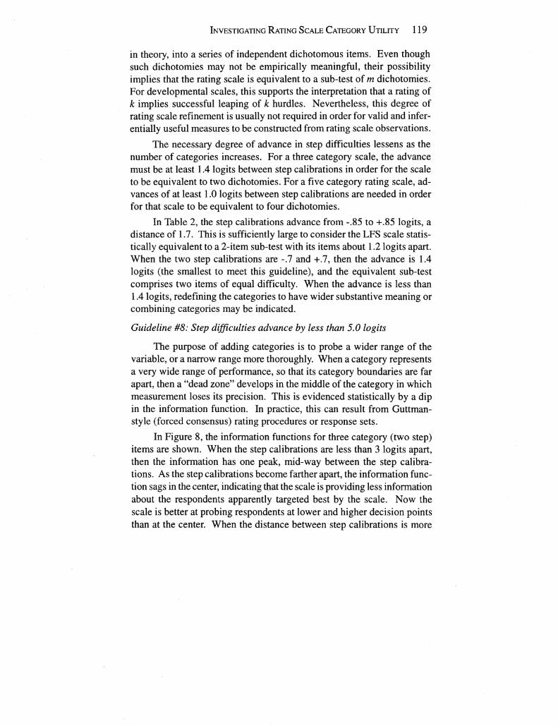
A sounder alternative is to use the variable map from the Participation scale which is reproduced in Figure 1 By looking at the map one could identify the specific summary score (transfonned score) that best represhysented the perfonnance profile for what was considered high participashytion Because the variable maps reflect the infonnation on relative item and rating difficulty one could decide the settings in which it was most important for participants to have achieved a minimum rating of 4 in order to be included in the high participation group Two possibilities are illustrated in Figure 1 In the first a lower criterion is set (dotted line) This criterion reflects a judgement that when the students total score indicates there are at least two settings in which 4 is the expected rating he or she is assigned to the high participation group A second choice (solid line) is to set a higher criterion Here the final cut score is set at the point where the student would be expected to have ratings of 4 in all settings
An important point here is that this alternative strategy for cut-score determination rests on the researchers clinical understanding of which profile best represents the outcome of interest for the particular study Thus rather than rely on more arbitrary groupings based on traditional statistical evidence such as frequency counts or the midpoint of a distrishybution the researcher can set a criterion that incorporates information regarding the difficulty of the items and the desired level of performance defined by the positive and less positive outcomes selected
Application Example 2 Interpreting the meaning of results
The focus of the study used for these examples was to identify predicshytors of good and poor outcomes with an ultimate aim of understanding pathshy
USING IRT VARIABLE MAPS 129
ITEM -10 0 30 5~ 7D 90 110
Regular Ed Class 2 is 4 5 6 Playgroundrecess 2 5 4 5 6 Transportation 1 2 i 5 6BathroamvToileting 2 ~ 4 5 6 Transitions 2 3 4 5 6
MealtimeSnacktime 2 3 5 4 5 6
-10 10 30 7D 90 051 Figure 1 Participation Variable Map (6 school setting items) Adapted from the School Function Assessment Copyrightcopy 1998 by Therapy Skill Builders a division of The Psychological Corporation Reproduced by permission All rights reserved
Note The two lines indicate potential cut-off points to dichotomize the Participation variable For the first option a lower scaled score is selected (dotted line) at the point where a student is expected to have a rating of 4 (Participation with occasional assistance) in at least two settings Once a student achieves this score he or she will be assigned to the high participation group For the second option (solid line) a higher criterion is set by choosing a cut-off score at the point where the student would have an expected rating of at least 4 in all settings
ways to successful participation and the variables that help identify those students most likely to benefit from rehabilitation services Because the ultishymate goal was to generate outcome predictions for individuals a Classificashytion and Regression Tree (CART) analysis approach (Breiman Friedman Olshen and Stone 1993) was chosen A full discussion of CART is beyond the scope of the present paper however the essential features will be deshyscribed as needed to understand this application example A complete disshycussion of the present study and its results is found elsewhere (Mancini1997)
CART is a non-parametric multivariate procedure that can be used to classify individuals into specified outcome categories The analysis proceeds through a series of binary recursive partitions or splits to select from a larger set of predictor variables those that considered in sequence provide the most accurate classification of the individuals in the sample This method is particularly helpful to identify interactions among predicshytor variables in situations where such interactions are likely but there is limited previous research to guide the analysis (See Falconer Naughton Dunlop Roth Strasser and Sinacore 1994 for an application of CART methodology in the analysis of stroke rehabilitation outcomes)
130 COSTER et al
Another valuable feature of CART is that for each predictor varishyable that is selected all potential divisions or values of the variable are tested to identify the one that best separates individuals into the groups of interest This cut-point can be useful for clinicians who want to use the CART decision tree to identify persons likely to have better or worse outcomes in a similar clinical context However for researchers intershyested in understanding the pathways to different outcomes it would be helpful if there were some means to ascertain why a particular cut-point might have been selected That is what distinguishes the performance of persons above and below that score level This is the situation where if scores are IRT -based measures application of the relevant variable maps may prove very useful
In the present example a CART analysis was conducted to examine predictors of school participation using the SFA Participation variable
0 10 20 30 40 50 70 80 90 100
Buttons sma II buttons 2 3 4 Fastens belt buckle 1 middot 2 3 4 SeparateshooKs zipper 1 2 3 4 Buttons 11 corresp 1 2 3 4 Secures shoes 1 2 3 4 Puts shoes on 2 middot 3 4 Puts socks onoff 2 4]
Puts on pullover top 1 2 4 Hangs clothes 1 2 3 4Removes shoes 2 3 4Removes pullover top 2 3 4 Zips and unzips 2 3 4 Lowers garment bottom 2 3 4 Puts on front-open top 1middot 2 3 4 Puts on hat 1middot 2 3 middot4 Removes front-open top 2 3 middot 4 Removes hat 2 3 4-
0 10 20 30 40 50 60 70 80 90 100
Figure 2 Clothing Management Variable Map (17 functional activity items) Adapted from the School Function Assessment Copyrightcopy 1998 by Therapy Skill Builders a division of The Psychological Corporation Reproduced by permission All rights reserved
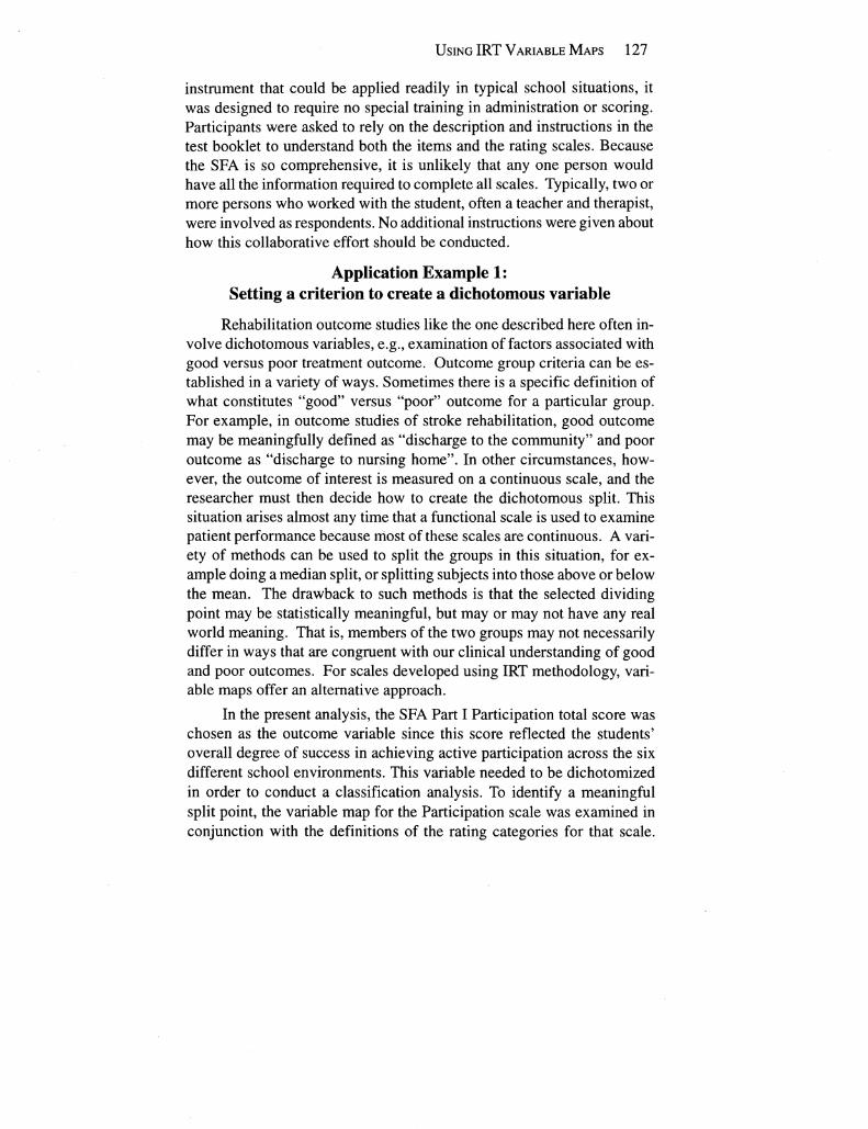
Note The solid line indicates the cut-point of 59 selected by the CART analysis The expected functional activity performance profile of students with scores below 59 is described by the ratings to the left of this line that of students above the cutshypoint is described by the ratings to the right of the line Results indicate that students may be classified into the high participation group even though they may still be expected to have difficulty (ie as indicated by ratings of 1 Does not perform or 2 Partial performance) on fine motor activities such as buttoning buttons
USING IRT VARIABLE MAPS 131
dichotomized as described above as the outcome measure and SFA Part III scaled scores as predictors The specific research question was which of the functional tasks examined in Part III are most informative in preshydicting high or low participation The first variable selected by the proshygram was the Clothing Management score with a cut point set at a score of 59 Although this result seemed counter-intuitive given the outcome focus on school participation a review of the content of this scale sugshygested that it was probably selected because it measures functional pershyformance in activities that require a variety of both gross motor and fine motor skills Thus the variable may be serving as an indirect measure of severity of physical disability (for more detailed discussion see Mancini 1997) However application of the variable map for this scale provided more insight into the result
The variable map for this scale is reproduced in Figure 2 and the selected cut point is identified with the solid vertical line The line idenshytifies the expected pattern of item performance associated with scores above (to the right) and below (to the left) of 59 Review of the items indicates that students with scores below 59 would be expected to have difficulty with the basic gross motor and postural control aspects of dressshying The profile suggests that these students are generally not able to consistently initiate andor complete (ratings lt3) lower body dressing activities such as raising and lowering pants or putting on and taking off shoes and socks nor can they do any significant portions of manipulative taskS (ratings of 1) In qmtrast students with scores above 59 manage the gross motor aspects of dressing relatively well although many would still be expected to have difficulty with fine motor aspects such as doing fasshyteners (eg expected ratings of 2)
This more in-depth interpretation of results supported by the varishyable map is valuable on several counts First examining the items on either side of the cut-point helped confirm the initial interpretation that the scale was selected because it provided an indirect measure of severity of mobility limitations This result makes clinical sense since severe mobility restrictions can pose significant challenges to active participashytion in school across a wide variety of contexts On the other hand the results also suggested that limitations in the performance of manipulative activities did not on their own significantly predict school limitations The latter result is somewhat surprising given the number and variety of fine motor activities (eg writing and other tool use eating activities) typically expected during the school day This result invites further reshy
132 COSTER et al
search into the question of what the minimum threshold of functional performance for school-related fine motor activities may be and the deshygree to which limitations in this area may be accommodated successfully through various adaptations This more precise definition of questions for future research would not have been possible without the additional information provided through examination of IRT variable maps
Discussion
This paper has presented two illustrations of research applications of variable maps to guide definition of outcome groups and to obtain a more in-depth understanding of results Both types of applications are relevant to a variety of other clinical and research situations where IRT -based scales are used For example clinical facilities and researchers analyzing patient outcomes may face similar questions of how best to describe positive and negative outcome groups If they are using IRT-based measures for which variable maps are available they can follow a similar rational procedure for deciding which cut-off point is most appropriate given their questions
The more common applications are those in which variable maps can enhance understanding of particular scores related to research or clinishycal outcomes For example rather than simply reporting the mean funcshytional performance score for a group of patients discharged from an intervention program one could use the variable map to describe the exshypected functional performance profile associated with that score and the proportion of patients who achieved that level or better Similarly deshyscriptive analyses of change over time in a particular patient group would be much more meaningful if the scores at admission and discharge were interpreted using variable maps in terms of the expected functional proshyfiles represented by each score For example consider an intervention program that enabled a substantial portion of students to achieve scores above 59 on the Clothing Management scale used in the previous exshyample In addition to reporting the average amount of change in the scaled score after intervention one could also describe the increased level of independent function that this change represents ie that these students are now able to manage basic dressing tasks more consistently on their own implying less need for assistance from the teacher In this context interpreting results using variable map information on the expected funcshytional performance profiles associated with pre and post scores can help to resolve debates over whether particular statistical differences in scores represent clinically meaningful change
USING IRT VARIABLE MAPS 133
References Breiman L Friedman JH Olshen RA and Stone CJ (1993) Classificashy
tion and regression trees NY Chapman and Hall
Coster WJ Deeney TA Haltiwanger JT and Haley SM (1998) School Function Assessment San Antonio TX The Psychological Corporation Therapy Skill Builders
Falconer JA Naughton BJ Dunlop DD Roth EJ Strasser DC and Sinacore JM (1994) Predicting stroke inpatient rehabilitation outcome using a classification tree approach Archives ofPhysical Medicine and Reshyhabilitation 75 619-625
Fisher WP (1993) Measurement-related problems in functional assessment American Journal ofOccupational Therapy 47331-338
Haley SM Ludlow LH and Coster WJ (1993) Clinical interpretation of summary scores using Rasch Rating Scale methodology In C Granger and G Gresham (eds) Physical Medicine and Rehabilitation Clinics of North America Volume 4 No3 New developments in functional assessment (pp 529-540) Philadelphia Saunders
Linacre JM and Wright BD (1993) A users guide to BIGSTEPS Raschshymodel computer program Chicago MESA Press
Ludlow LH HaleySM and Gans BM (1992) A hierarchical model offuncshytional performance in rehabilitation medicine Evaluation and The Health Professions 15 59-74
Ludlow LH and Haley SM (1995) Rasch modellogits Interpretation use and transformation Educational and Psychological Measurement 55 967-975
Mancini M C (1997) Predicting elementary school participation in children with disabilities Unpublished doctoral dissertation Boston University
Wright BD Linacre JM and Heinemann Aw (1993) Measuring funcshytional status in rehabilitation In C Granger and G Gresham (eds) Physical Medicine and Rehabilitation Clinics ofNorth America Volume 4 No3 New developments in functional assessment (pp 475-491) Philadelphia Saunders
JOURNAL OF OUTCOME MEASUREMENT 3(2)134-161
Copyright 1999 Rehabilitation Foundation Inc
Measuring Pretest-Posttest Change with a Rasch Rating Scale Model
Edward W Wolfe University ofFlorida
Chris WT Chiu Michigan State University
When measures are taken on the same individual over time it is difficult to determine whether observed differences are the result of changes in the person or changes in other facets of the measurement situation (eg interpretation of items or use of rating scale) This paper describes a method for disentangling changes in persons from changes in the interpretation of Likert-type questionnaire items and the use of rating scales (Wright 1996a) The procedure relies on anchoring strategies to create a common frame of reference for interpreting measures that are taken at different times and provides a detailed illustration of how to implement these procedures using FACETS
Requests for reprints should be sent to Edward W Wolfe 1403 Norman Hall University of Florida Gainesville FL 32611 e-mail ewolfeufleduThis research was supported by ACT Inc and a post-doctoral fellowship at Educational Testing Service The authors thank Carol Myford Mark Reckase and Hon Yuen for their input on a previous version of this manuscript A previous draft of this paper was presented in March of 1997 at the International Objective Measurement Workshop 9 in Chicago IL
MEASURING PRETEST-POSTIEST CHANGE 135
Measuring Pretest-Posttest Change with a Rasch Rating Scale Model
Measuring change over time presents particularly difficult challenges for program evaluators A number of potential confounds may distort the measurement of change making it unclear whether the observed changes in the outcome variable are due to the intervention or some other effect such as regression toward the mean (Lord 1967) maturation of particishypants or idiosyncrasies of participants who drop out of the program (Cook and Campbell 1979) When rating scales or assessment instruments are used to measure changes in an outcome variable additional confounds may be introduced into the evaluation process For example participants may improve their performance on an assessment instrument that is used as both a pre-test and post-test because of familiarity with the test items (Cook and Campbell 1979) Alternatively when changes are measured with Likert-type questionnaires participants may interpret the items or the rating scale options differently on the two occasions (Wright 1996a)
This article describes and illustrates an equating procedure proposed by Wright (l996a) that can be applied to rating scale data to compensate for the latter of these potential confounds to measuring change over time That is we describe a method for reducing the effect that changes in parshyticipants interpretations of questionnaire items and rating scale options may have on the measurement of change on the underlying construct We outline the procedures for making this correction illustrate how these procedures are carried out and demonstrate how the employment of these procedures can lead to the discovery of changes that would not be apparshyent otherwise By implementing this equating procedure evaluators can eliminate at least one potential threat to the valid interpretation of changes in attitudes or opinions as measured by Likert-type questionnaires
Theoretical Framework
In many program evaluation settings evaluators are interested in measuring changes in the behaviors or attitudes of non-random samples of participants who are drawn from a population of interest Changes in the measures of the outcome variable are typically attributed to participashytion in the program in question Of course numerous threats to the validshyity of this inference exist and each of these threats highlights a potential confound that must be taken into account when designing an evaluation collecting and analyzing data and interpreting the results These threats
136 WOLFEANDCHIU
to the validity of interpretations that are drawn from a program evaluation may relate to statistical validity (the accuracy of the statistical inferences drawn about the relationship between the program and the outcome varishyable) construct validity (the accuracy of the inferred relationship between the measurement procedures and the latent construct they are intended to represent) external validity (the accuracy of the inferred relationship beshytween the participants and the population that they are intended to represhysent) or internal validity (the accuracy of the theory-based inferences drawn about the relationship between the program and the outcome varishyable) Methods for avoiding or reducing each of these threats to drawing valid inferences are outlined by Cook and Campbell (1979)
The problem addressed by this article represents one of several poshytential threats to internal validity That is we are concerned with whether observed changes in the outcome variable are truly caused by participashytion in the program or whether observed changes can be attributed to other variables that are byproducts of the evaluation setting In a program evalushyation threats to internal validity may arise when changes in participants can be attributed to maturation changes in participants familiarity with the measurement instrument mortality of participants the procedures used to assign participants to treatments statistical regression toward the mean or changes in the measurement instrument rather than the treatment itself The threat to internal validity that we discuss arises when Likert-type questionnaire items are used to measure attitudinal changes More speshycifically we are concerned with the degree to which changes in the way participants interpret questionnaire items and use rating scales confounds the measurement of changes in attitudes or opinions
Prior research in this area has shown that participants interpretashytions of items or rating scales may change over time and that this is a common concern for those who use questionnaires to measure outcome variables For example Zhu (1996) investigated how childrens psychomotoric self-efficacy changes over time In this study children completed a questionnaire designed to measure the strength of their conshyfidence about their abilities to perform a variety of physical exercises The results of this study indicated that some of the activities were pershyceived as being less difficult to perform relative to the remaining activishyties over repeated administrations of the questionnaire Such differential functioning of items over time threatens the validity of interpretations that might be drawn from the results of Zhus study
MEASURING PRETEST-PaSTIEST CHANGE 137
In order to evaluate changes in persons over time participants inshyterpretations of the items and rating scales that are used to measure this change must be stable across multiple administrations of the questionshynaire Only if interpretations of items and rating scales demonstrate such stability can differences between measures of the persons be validly inshyterpreted (Wilson 1992 Wright 1996b) To further exacerbate the probshylem summated composite scores are not comparable across time when items are added removed or reworded items are skipped by some subshyjects or response options change from pre-test to post-test-all problems that are common with multiple questionnaire administrations (Roderick and Stone 1996) In order to mitigate some of these problems scaling methods are often used to place measures from different administrations of a questionnaire onto a common scale
Rasch Rating Scale Model
The Rasch Rating Scale Model (RSM) is an additive linear model that describes the probability that a specific person (n) will respond to a specific Likert-type item (i) with a specific rating scale category (x) (Andrich 1978) The mathematical model for this probability (Equation 1) contains three parameters the persons ability (~n) the items difficulty (0) and the difficulty of each scale step (ie the threshold between two adjacent scale levels x and x-I) (t) Calibration of questionnaire data to
J this model results in a separate parameter estimate and a standard error for that estimate for each person item and scale step in the measurement context
(1)
where P(Xni = x) is the probability that a person n responds with rating scale category x to item i which has m+1 response options
The fit of these estimates to the RSM (ie model-data fit) can be evaluated using a standardized mean square fit statistic as shown in Equashytion 2 (Wright and Masters 1982) When the data fit the RSM t has a
e
mean near zero and a standard deviation near one Estimates with It 1gt200 e
exhibit poor fit to the model and should be further examined to determine
138 WOLFE AND CHIU
whether there are problems with the scores associated with that particular person item or rating scale step
(2)
where ve is the weighted mean of the squared residuals (weighted by their variances) of the observed data from their expected values and qe is the model standard deviation of the weighted mean square
An important feature of the RSM is that it allows one to evaluate the extent to which item calibrations are stable across samples of pershysons or the extent to which person measures are stable across samples of items (ie to determine the invariance of parameter estimates) This feature is useful when comparing two groups of persons who respond to the same set of items or equating two tests (each composed of different items) that are taken separately by a single group of people In the present context invariance evaluation is useful because it allows one to detershymine the extent to which item calibrations and person measures are stable across two measurement occasions The stability of two parameter estishymates ( 81 and eJ that are obtained on different occasions is evaluated by examining the standardized difference (Equation 3) between the two estimates (Wright and Masters 1982) The standardized differences for a population or item pool that conform to the RSM have an expected value of 000 and an expected standard deviation of 100 Large deparshytures in observed data from these expected values indicate estimates that are less stable over time than would be expected
(3)
Examining Change Over Time with the Rating Scale Model
Measuring change over time requires a stable frame of reference and differential functioning of items and rating scales disrupts the establishshyment of such a frame of reference In order to measure changes in the pershyformance of persons across time other changes in the measurement framework must be eliminated or controlled There are several methods for accomplishing this (Wright 1996b) For example facets other than the pershysons may be assumed to be constant by forcing the elements of each facet to
MEASURING PRETEST-PaSTIEST CHANGE 139
STEP 1
Evaluate the rating scale and item invariance
with separate analyses of Time 1 and Time 2 Data
1 versus 2 and Di versus Di2
~ STEP 2
Create common scale calibrations (c) by stacking Time 1 amp Time 2 data
and treating persons as unique at each time point
~ STEP 3
Obtain corrected person measures (3nlJ and
corrected item calibrations (Die) for Time 1 data
with the rating scale anchored on c
1 STEP 4
Obtain corrected person measures (3n2c) for Time 2 data
with the rating scale anchored on e
and the 0 stable items from Step 1 anchored on Dile
Note Person change is evaluated via 3nle-3n2c
1 STEPS
Obtain corrected item calibrations (Di2c) for Time 2 data
with the rating scale anchored on ltxc
and the persons anchored on 3n2c
Note Item change is evaluated via Dilc-Di2c
Figure 1 Steps for creating a frame of reference using Rasch measurement
140 WOLFE AND eHIU
remain fixed Alternatively facets that exhibit noticeable change from one occasion to another may be assumed to be truly different indicators of the construct in question and may therefore be treated as being completely different elements at each time Finally a compromise can be achieved beshytween different administrations of an instrument by creating an average frame of reference and allowing facets to vary about that average
The method we describe was originally proposed by Wright (1996a) and this method creates a common frame of reference by assuming that some elements of the measurement situation remain constant and by alshylowing others to vary over time Many researchers desire to identify whether differences demonstrated by specific items or persons are large enough to be of importance and the method presented in this article alshylows for such a distinction Once a common frame of reference has been created differences between person measures or between item calibrashytions at each measurement occasion can be evaluated by examining the standardized differences of the parameter estimates produced for each occasion The method is described here as a five step procedure as porshytrayed in Figure 1
Step 1 Evaluate Rating Scale and Item Invariance
The first step in using the RSM to measure change over time is to determine whether interpretations of the scale steps and the items are stable across the two measurement occasions If the item and step calibrations do demonstrate stability over time (ie they are invariant) then differshyences between person measures at the two occasions are valid indicators of changes in persons over time (ie they are free from potential conshyfounding due to changes in interpretations of items or uses of rating scales) However if the scale step and item calibrations are not invariant over time then the researcher must disentangle the changes in the scale steps items and persons to determine which elements of the measurement conshytext are indeed changing (Steps 2 through 5)
To determine whether the scale step or item calibrations are invarishyant over time one must generate two data sets-one containing the reshysponses of each person (n) to each item (i) at Time 1 and the other containing the responses of each person to each item at Time 2 The layshyout of these data sets is shown in Figure 2 Item and step calibrations as well as person measures are obtained for each data set separately so that there is a pair of estimates one for Time 1 and one for Time 2 for each scale step (tjl amp tJ) each item laquo amp 3) and each person (~nl amp ~n2)
MEASURING PRETEST-PaSTIEST CHANGE 141
1 1- xIII x2l 111 1H
2 1- x211 x221 middotmiddotmiddotx2l1Timel
N 1- xNll xN21 middotmiddotmiddotxNIl
1 1- xI12 xI22middotmiddotmiddot X1I2] 2 1- x212 x222 middotmiddotmiddotx212
Tlme2 r
N 1- xNI2 xN22 middotmiddotmiddotxNl2
Figure 2 FACETS Data Layout for Step 1 The first column shows the examinee the second column shows the item range N is the number of examinees and I is the number of items
(where ~nl refers to the measure for person n at Time 1 and ~n2 refers to the for person n measure at Time 2)
To evaluate item and step calibration invariance over time one comshypares the pair of calibrations for each element of these two facets That is one compares tjl and tj2 for each step level and compares Oil to 0i2 for each item This comparison can be made using the standardized difference of the two estimates (Equation 3) Items or scale steps that exhibit large difshyferences between their Time 1 and Time 2 calibrations (eg Izlgt 200) are not invariant over time (ie they are unstable) Such differences between the way the scale steps were used or the items were interpreted at each occasion may confound any inferences that are drawn based on observed differences in the person measures for Time 1 and Time 2 and the reshysearcher must make corrections (Steps 2 through 5) For now note that there are 0 invariant items If there are no large differences between step and item calibrations from the two occasions then it is safe to interpret the differences between the person measures from the two occasions as indicashytors of change in persons over time Again this can be done by examining the standardized differences (Equation 3) between the two measures for each person (~nl amp ~n2)middot
Step 2 Create Common Scale Calibrations
If the analyses in Step 1 reveal that any of the step or item calibrashytions are not stable across time then there is a need to constrain this
142 WOLFE AND CHID
variability before interpreting observed changes in person measures In order to measure change one must assume that at least one facet of the measurement context remained stable The current method relies on the assumption that the rating scale remained stable by using the average value for the scale steps to create the measurement framework Thus this method assumes that a common underlying equal-interval scale adequately porshytrays the data and that departures from that underlying scale are due only to random fluctuations
Therefore the second step in measuring change over time is to creshyate common step calibrations so that person measures and item calibrashytions from Time 1 and Time 2 can be compared on a common underlying rating scale To accomplish this we allow persons to float from Time 1 to Time 2 and items are assumed to be invariant from Time 1 to Time 2 That is persons are treated as being different objects of measurement on each of the two occasions This means that the two data sets from Step 1 must be reconfigured by assigning two unique identifiers to each pershyson-one for Timel responses (n1) and one for Time 2 responses (n2) and appending them (ie stacking them to create a single data set) The format of the reconfigured data is shown in Figure 3
11 1- x1111 x1l21 xllIl
21 1- x2111 x2121 x21Il
N1 1- xN111 xNl21 xNlIlStacked
12 1- x1212 xl222 x1212
22 1- x2212 x2222 bull x2212
N2 1- xN212 xN222 xN212
Figure 3 FACETS Data Layout for Step 2 The first column shows the examinee the second column shows the items N is the number of examinees and I is the number of items
This stacked data set is analyzed to obtain step calibrations that are consistent with person performance and item functioning across both ocshycasions The values of these common scale estimates (t ) are used in Steps
JC 3 through 5 as anchors for the scale steps Analysis of the stacked data set also produces a single set of item calibrations and two separate measures
MEASURING PRETEST-PaSTIEST CHANGE 143
for each person-one portraying the person at Time 1 and another porshytraying the person (as a different person) at Time 2 These item calibrashytions and person measures are ignored Note that the calibrations from this step for the items that were identified as showing instability over time in Step 1 should show greater misfit to the RSM (Wright 1996b)
Step 3 Correct the Time 1 Estimates
Once a common rating scale has been created for the two occasions that scale is used as a frame of reference for the Time 1 and Time 2 data sets In Step 3 of the procedure the Time I data are re-analyzed using the step calibrations from Step 2 (ie tj ) as anchors for the rating scale This results in two sets ofestimates a) corrected person measures for all persons (R 1 ) and b) corrected item calibrations for all items (01 ) These estimates tJ n C I C
are referenced to the common scale that was created in the Step 2 analyses and they are used as the basis for measuring change in Steps 4 and 5
Step 4 Correct the Time 2 Person Measures
In Steps 2 and 3 a frame of reference was created for interpreting changes in person measures at Time 2 by creating a rating scale that is common to both occasions and determining the corrected Time 1 person measures and item calibrations In Step 4 the Time 2 data are re-analyzed by anchoring the steps on the common-scale values obtained in Step 2 (ie tj ) and anchoring the a invariant items from Step 1 on the corrected item calibrations from Step 3 (Oole) The I-a items that were found to be unstable from one occasion to the next in Step 1 however are not anshychored (ie they are allowed to float)
The Step 4 analyses produce corrected person measures at Time 2 (~n2) that are referenced to a rating scale that is common to both Time 1 and Time 2 and a set of items that are invariant across time Any differshyences between these corrected person measures and the corrected meashysures obtained in Step 3 (~n1) indicate changes in persons rather than interpretations of items or uses of the rating scale over time For each person the corrected Time 1 measure (~n1c) and the corrected Time 2 measure (~n2c) can be compared using the standardized difference as shown in Equation 3 Persons that exhibit large variability (eg Izlgt 200) have changed over time The analysis also produces calibrations for the I-a unstable items (ie the items that were allowed to float-0(l_Ol2) These calibrations are ignored
144 WOLFE AND CHIU
Step 5 Correct the Time 2 Item Calibrations
The final step in the procedure is to determine the extent to which item functioning changed over time while controlling for changes in pershyson measures In Step 5 the Time 2 data are re-calibrated by anchoring the scale steps on the joint calibrations obtained in Step 2 (tj ) and anchorshying the person measures on the corrected Time 2 estimates from Step 4 (~n2c) All items are allowed to float This analysis results in item calibrashytions (for all items) at Time 2 (Oi2) that are corrected for changes in both the interpretation of the rating scale and the performance of people To determine how much item functioning changed across occasions the corshyrected Time 1 item calibrations (Oil) are compared to the corrected Time 2 item calibrations (oi2e) The comparison can be made by computing the standardized differences between these two estimates (Equation 3) This comparison is free from potential confounds due to changes in the use of the rating scale or the performance of persons across time It is important to note that calibrations for items that were found to be unstable over time in the Step I analyses have been treated as different items in the estimashytion of person measures regardless of how much their corrected calibrashytions differ
Example
The remainder of this article illustrates how this procedure can be applied to the measurement of change in questionnaire data We demonshystrate this technique on data that are typical of many program evaluations (ie single group pretest intervention posttest) Our analyses emphashysize how using the procedure results in different interpretations of how persons and items change over time
Participants
The data for our illustration come from mathematics science and language arts teachers from 14 public and private secondary schools in different regions of the United States These teachers participated in a nine-month program designed to help them develop portfolio assessments Approximately 12 teachers from each school participated in the program (n = 168) At the beginning of the school year (in September) teachers responded to a questionnaire designed to assess the strength with which teachers perceive potential barriers to the implementation of a portfolio assessment program to be problematic (Wolfe and Miller 1997) After
MEASURING PRETEST-POSTIEST CHANGE 145
participating in the program for an academic year (in June) teachers comshypleted the questionnaire a second time A comparison of a teachers reshysponses from September (Time 1) with the responses provided in June (Time 2) was interpreted as a measure of change in the teachers percepshytion of barriers to the implementation of portfolio assessments Complete data for Time 1 and Time 2 were available for 117 of the 168 teachers who participated in the program (a 30 attrition rate)
Instrument
The questionnaire asked teachers how problematic they perceived 30 potential barriers to the implementation of a portfolio assessment sysshytem to be The barriers referenced issues such as the amount of time reshyquired to use portfolios resistance from people to the idea of using portfolios the difficulty of assigning scores to portfolio entries changes in instruction that are required when portfolios are used and the availshyability of resources for using portfolio assessment Each barrier was forshymatted as the stem for a four-point Likert-type item Teachers responded to each barrier by indicating whether the barrier is a(n) unlikely minor difficult or serious problem For each of the 30 barriers teachers indishycated the option that best describes the difficulty of that specific barrier Unlikely problems were defined as those that would likely have no impact on the teachers use of portfolios Minor problems were those that may cause the teacher to use portfolios differently than they would be used in an ideal situation Difficult problems were defined as problems that may cause the teacher to reconsider using portfolios in his or her classroom Serious problems were those that would cause the teacher not to use portshyfolios at all
Analyses and Results
These data were analyzed with a Rasch RSM For substantive meanshying all facets were scaled so that higher logit values were associated with more difficult portfolio implementation That is higher values of teacher measures were associated with the perception of portfolio implementashytion as being more difficult and higher values of barrier and rating scale step calibrations were associated with barriers that are more difficult to overcome In each of the following sections we detail the steps of the anchoring method described by Wright (l996a) Prior to illustrating the five steps however the fit of the data to the RSM is evaluated
146 WOLFE AND CHru
Evaluating Fit
For Step 1 the data were placed in two data sets-one containing the teachers responses from September (Time 1) and the other containshying teachers responses from June (Time 2) (see Figure 2) Each data set contained three variables a) teacher (person) identifier b) barrier (item) identifier and c) the teachers response (rating) to that barrier In our deshyscription we use FACETS (Linacre 1989) to obtain parameter estimates for these data sets It should be noted however that these analyses can be performed using any item response software that allows for the analysis of rating scale data and the anchoring of measurement facets The two data sets one from each of the two occasions were calibrated on separate FACETS analyses An example FACETS command file for performing Step 1 on the September data is shown in Appendix A A similar comshymand file is written for the June data These analyses result in two sets of barrier calibrations and teacher measures-one for the September data and one for the June data
To evaluate the fit of the data to the model the standardized mean square fit statistics (Equation 2) for the parameter estimates of each teacher and barrier were examined at each occasion Teachers and barriers with fit statistics greater than two were flagged as potential problems Howshyever no teachers or barriers were eliminated from the analyses based on misfit because inspection of their response pattems revealed no conspicushyous anomalies Sixteen of the teachers (14) showed poor fit to the model in the September data and twelve (10) showed poor fit in June Three of the barriers in our questionnaire (10) had large fit statistics for the Sepshytember data and only one (3) showed poor fit in June
Step 1 Evaluate Rating Scale and Barrier Invariance
As described in the previous section in Step 1 the September and June responses were analyzed separately so that each teacher barrier and rating scale step received a pair of parameter estimates-one for Septemshyber and one for June The pair of estimates for each teacher barrier and rating scale step are referred to here as ~nl and ~n2 Oil and 0i2 and tjl and tj2 respectively In subsequent sections these estimates will also be reshyferred to as uncorrected estimates To determine whether differences beshytween ~nl and ~n2 are valid indicators of change in teacher measures over time we computed the standardized differences (Equation 3) between each pair of step calibrations (t I and t) and each pair of barrier cali brashy
I J
MEASURING PRETEST-PaSTIEST CHANGE 147
tions (Ojl and OJ) The parameter estimates for September and June their standard errors and the associated standardized differences are shown in Table 1 and Figure 4
The analyses from Step 1 reveal that there are large differences in the way that the rating scale steps were used at September and June as indicated by the large standardized difference for two of the three scale
Table 1
Rating Scale Step Calibrations from Step 1 for September and June
Scale Step tjl Logit tjl Error tj2 Logit tj2 Error z
oto 1 -182 004 -124 004 -1025
1 to 2 005 005 012 005 -099
2 to 3 177 010 113 008 500
Mean 000 006 000 006 middot208
(SD) (180) (003) (119) (002) (768)
Note tjl represents the rating scale step calibrations obtained in Step 1 for Sepshytember and tj2 represents the rating scale step calibrations obtained in Step 1 for June Izlgt200 is considered large enough to indicate unstable uses of rating scale steps across occasions
2
September
-2 2
June
Figure 4 Scatter plot of uncorrected September and June barrier calibrations
148 WOLFE AND CHIU
step calibrations (Table 1) Specifically the difference between Septemshyber and June scale steps for the 0 to 1 and the 2 to 3 transitions are so much larger than their standard errors that their invariance across time is suspect Furthermore several of the barriers showed unexpectedly large changes in their calibrations over the two administrations of the questionshynaire In fact 7 of the 30 barriers (23) have absolute standardized difshyferences greater than 200 (ie 0 =23) as evidenced by the points falling outside of the 95 confidence bands shown in Figure 4 This is a large percentage of barriers when compared to the expectation derived from the standard normal distribution (about five percent) The largest change in barrier calibrations indicated as point A on the scatterplot was 449 standard errors (from -058 to -168 logits) In addition the standard deshyviation of the standardized differences (180) is considerably larger than the expected value of 100 These statistics suggest that differences in the functioning of barriers and rating scale steps over time may cloud any interpretations that we make of differences in teacher measures so our example proceeds with Steps 2 through 5 of Wrights (1996a) correction procedure
Step 2 Correct the Scale Calibrations
In Step 2 of the procedure a common rating scale is created so that teacher attitudes and barrier severity estimates from September and June can be estimated in a common frame of reference To this end we stack the two data sets from Step 1 reassigning teacher identifiers to each teacher for the June responses (as shown in Figure 3) In our example we simply added 1000 to the original identifier (as shown in the example FACETS command file presented in Appendix B) Because this step of the analysis portrays each teacher as being a different person in June than in Septemshyber and allows barriers to remain stable across administration of the quesshytionnaire the output of this command file results in a pair of measures for each teacher and a single calibration for each barrier All of these values are ignored The rating scale step calibrations ( ~) from this analysis howshyever are of interest and will be utilized as anchor values for the remaining steps of the procedure Table 2 compares the scale step calibrations from Step 1 of the procedure to those obtained from Step 2 As one would expect the values from Step 2 (ie the step calibrations for the scale that are common to September and June) are between the two values obtained in Step 1 (ie the step calibrations for the separate September and June scales) In addition because each calibration is based on a larger number
MEASURING PRETEST-POSTIEST CHANGE 149
Table 2
Rating Scale Step calibrations from Step 1 and Step 2
Scale Step tjl Logit tjl Logit tjc Logit tjc SE
oto 1 -182 -124 -146 003
1 to 2 005 012 010 003
2 to 3 177 113 136 006
Mean 000 000 000 004
(SD) (180) (119) (141) (002)
Note tjl represents the rating scale step calibrations obtained in Step 1 for September tj2 represents the scale step calibrations obtained in Step 1 for June and tjc represents the scale step calibrations obtained in Step 2 for the comshybined September and June data set (ie the common scale)
of observations the standard errors of these calibrations are smaller than those for the Step 1 calibrations
Step 3 Corrected September Estimates
In Step 3 corrected estimates are obtained for teachers (~n) and barriers (Oil) in September by anchoring rating scale steps on the values obtained in Step 2 (tjJ Appendix C shows an example FACETS comshymand file for this analysis Note that the command file is the same as the command file used in Step 1 with the exception that rating scale steps are now anchored on their r values The data file is the same one used for the
JC
September analysis in Step 1 The Step 3 analyses result in two sets of values for the September data The corrected teacher measures (~n) and the corrected barrier calibrations (Oil) are used as the basis for measuring changes in teachers and barriers in Steps 4 and 5 These estimates are also referred to as the corrected September estimates
Step 4 Correct the June Teacher Measures
In Step 4 the common rating scale step calibrations from Step 2 (tj) and the corrected barrier calibrations obtained in Step 3 (OJ Ie) for the 0 (23) items that were found to be invariant across time in the Step 1 analyshyses (referred to here as 001) are used as anchors so that corrected teacher measures (~n2e) can be estimated for the June data As shown in Appendix D the seven barriers that were found to be unstable across time in Step 1
150 WOLFE AND eHIU
are not anchored (ie they are allowed to float) Note that new calibrashytions (0(100)2) are obtained for these barriers in Step 4 but these values are ignored Otherwise the procedures for analyzing the June data are the same as they were in Step 1 The resulting teacher measures (~n2) have been corrected for changes in perceptions of barriers and uses of the ratshying scale over time through this anchoring process As a result a comparishyson of the corrected June teacher measures (~n2c) with the corrected September teacher measures (~nlc) reveals how people have changed over time without confounding from changes in barrier or rating scale funcshytioning This comparison can be made by examining the standardized difshyference (Equation 3) for each teachers pair of corrected measures
Comparison of Uncorrected and Corrected Teacher Measures
Figure 5 displays the uncorrected and corrected measures for the 117 teachers in this study This scatter plot shows that overall the stanshydardized differences that were based on the corrected teacher measures were greater than those based on the uncorrected measures This is evishydent from the fact that the majority of the points fall above the identity line in Figure 5 That is teachers appear to have a more positive view as a result of participation in the program when the corrected measures are considered For example the teacher represented by point A had a
7
5
Zuncorrected
-7 -5 -3 5 7 ~~ ~
- -3 C
A
-5
Zeorrectoo-7
Figure 5 Scatter plot of uncorrected and corrected teacher standardized differences
MEASURING PRETEsT-PaSTIEST CHANGE 151
Z d = -578 and a z d = -540 Although there were only minor uncorrecte correcte
differences in most of the teacher standardized differences that were based on the uncorrected and the corrected measures (r = 99) the correction method made noticeable differences for some teachers This is particularly true for teachers who had positive standardized differshyences (ie showed a decreased sensitivity to barriers between the preshytest and posttest) as evidenced by the fact that the points are more dispersed in the upper right quadrant of Figure 5 As shown the teachshyers included in subset B are more dispersed than are other teachers in the sample As for changes in individual teachers standardized differshyences the largest discrepancy between teacher standardized differences between the uncorrected and corrected teacher measures was 097 (ie Z d = -077 and Z d = -174) indicated in the scatterplot asuncorrecte correcte
point C
Table 3 summarizes how the application of the method for measuring change influenced the distributions of teacher measures This table shows
Table 3
Uncorrected and Corrected Teacher Measure Summary Statistics
Statistic Uncorrected Measures Corrected Measures
Number with Fitgt 2 29 (12) 26(11)
Mean (z) -094 -053
Number with Significant z 57 (49) 54 (46)
SD (z) 243 233
Note Number with fitgt 2 represents the number of teachers with large fit statistics summed across both occasions Therefore the percent shown is the total number of misfitting teachers divided by 234 (117 x 2) Mean (z) is the average standardized difference across the 117 teachers and SD (z) is the standard deviation of the standardized differences Number with significant z represents the number of teachers with absolute standardized differencesgt 2
that the utilization of the correction method resulted in slightly fewer misfitting teachers ( t d = 12 t d = 11 ) In addition the corshyuncorrec e corree e
rection method also resulted in smaller differences between pretest and posttest measures as evidenced by the mean standardized difference (Mean zuncorrected =-094 Mean zcoITected =-053) As a result we would draw someshywhat different conclusions about the amount of change that teachers exhibshyited depending on whether we interpret the uncorrected or the corrected
152 WOLFE AND CHIU
measures This observation is supported by the fact that a smaller percent of the teachers corrected absolute standardized differences were greater than two ( ted = 49 d =46) Not only would our interpretation
uncorrec correcte
of the amount of change exhibited by the group of teachers change but so would our interpretation of which teachers changed Comparison of the standardized differences revealed that different conclusions would be drawn about 13 (11 ) of the teachers based on the uncorrected and corrected stanshydardized differences Of course the majority of these teachers had smaller standardized differences when their measures were corrected
Step 5 Correct the June Barrier Calibrations
In Step 5 the common rating scale step calibrations from Step 2 (tj )
and the corrected person measures for June obtained in Step 4 (~n2c) are used as anchors so that corrected barrier calibrations can be estimated for the June data As shown in the example command file in Appendix E this anchoring is the only difference between the analyses of the June data for Steps 1 and 5 The resulting barrier calibrations (Oi2) have been corrected for changes in teachers and uses of the rating scale over time The corshyrected June barrier calibrations can be compared to the corrected calibrashytions for September (Oil) obtained in Step 3 to identify how the perception of barriers changed over time As in the previous analyses this comparishyson is made by examining the standardized difference (Equation 3) for each barriers pair of corrected calibrations
Comparison of Uncorrected and Corrected Barrier Calibrations
Figure 6 displays the uncorrected and corrected calibrations for the 30 barriers in this study This scatter plot shows that there were larger differshyences between the standardized differences that were based on the uncorshyrected and the corrected calibrations than for the teacher measures as evidenced by the wider dispersion of points around the identity line Howshyever the correlation between corrected and uncorrected standardized difshyferences for barrier calibrations is still strong (r = 93) albeit somewhat inflated by the outlier represented by point A on the scatterplot This reshysulted in changes in individual barriers standardized differences as large as 142 (ie zuncorrectcd =-152 and zconected =-294 point B) depending on whether the uncorrected and corrected calibrations are considered
Table 4 summarizes how the application of the method for measurshying change influenced the distributions of barrier calibrations This table
MEASURING PRETEST-PaSTIEST CHANGE 153
6 A---
4
2
corrected
-6 -4 -2 2 4 6 -2
t -4
B
-6 Zcorrected
Figure 6 Scatter plot of uncorrected and corrected barrier standardized differences
Table 4
Uncorrected and Corrected Barrier Calibration Summary Statistics
Statistic Uncorrected Calibrations Corrected Calibrations
Number with Fitgt 2 4 (7) 2 (3)
Mean (z) -001 -009
Number with Significant z 7 (23) 7 (23)
SD (z) 180 188
Note Number with fitgt 2 represents the number of barriers with large fit stashytistics summed across both occasions Therefore the percent shown is the total number of misfitting barriers divided by 60 (30 x 2) Mean (z) is the average standardized difference across the 30 barriers and SD (z) is the standard deviashytion of the standardized differences Number with significant z represents the number of barriers with absolute standardized differencesgt 2
shows that the utilization of the correction method resulted in fewer misfitting barriers ( d =7 I = 3) In addition the corshyuncorrecte correctec
rection method also resulted in larger differences between pretest and posttest measures as evidenced by the mean standardized difference (Mean
154 WOLFE AND eHIU
Z d =-001 Mean Z d =-009) Again this result would lead us to uncorrecte corrccte
draw somewhat different conclusions about the nature of change in this study depending on whether we interpret the uncorrected or the corrected barrier calibrations-with the corrected measures we would say that teachshyers changed less and barriers changed more than they did when uncorshyrected values are considered And as was true for the teacher measures we would draw different conclusions about several of the individual barshyriers based on the uncorrected and corrected standardized differences Decisions concerning a total of six of the barriers (20) would be differshyent (half moving from significant to non-significant and half moving from non-significant to significant)
Conclusions
We have illustrated a procedure for removing potentially-confoundshying sources of variability from the measures of changes in persons over time Application of this procedure to the data in our example revealed four things about our perception of change in these data that were not apparent when this correction procedure was not applied First use of this procedure reduced the perceived overall change exhibited by this group of teachers That is depending on whether teacher measures were corshyrected or not a different magnitude of change in teacher measures from pretest to posttest was observed Second the procedure resulted in changes in the perception of which teachers changed over time In the example gi ven here we would draw different conclusions about 11 of the teachshyers as a result of applying the procedure Third the application of the procedure resulted in better fit of the teacher measures to the RSM By removing the confounding of changes in perceptions of barriers from the teacher measures and fluctuations in the use of the rating scale we were able to produce better measures of our teachers Finally we were able to detect changes in the perceptions of items over time that were not apparshyent without the correction procedure In fact we would draw different conclusions about 20 of the items after applying the correction proceshydure to our data
Overall this procedure seems useful for disentangling changes in the item functioning and rating scale use from changes in person perforshymance when Likert-type questionnaires are used to measure the impact that a program has in participants As a result the procedure could prove useful for program evaluators who are interested in measuring changes in attitudes and opinions We suggest four directions for further exploration
MEASURING PRETEST-POSTIEST CHANGE 155
of this procedure One direction would be to determine how well the method can be adapted to multi-faceted measurement contexts or to measurement models based on different response structures (eg partial credit modshyels) Often program evaluations are ongoing and involve measuring changes across several consecutive years so a second direction for future work might involve extending this correction procedure to settings with more than two measurement occasions Third it would be interesting to compare this method to other methods for disentangling sources of change in questionnaire data For example Chang and Chan (1995) identified four Rasch-based methods for measuring change that are distinct from the one presented in this article Comparison of these methods would reshyveal consistencies and differences in the ways that change is depicted Of course because there are multiple methods such a comparison would probably lead to conflicting results Therefore we suggest a fourth direcshytion for future research concerning the variety of models for measuring change over time We believe that any work that is based on these models is incomplete without evidence that the change that is being detected is indeed true change As a result we believe that it will be necessary to use simulations to determine the adequacy with which of each of the variety of methods recovers true change over time
References Andrich D (1978) A rating formulation for ordered response categories
Psychometrika 43 561-573
Chang We and Chan e (1995) Rasch analysis for outcome measures Some methodological considerations Archives ofPhysical Medicine and Rehabilishytation 76 934-939
Cook Te and Campbell DT (1979) Quasi-experimentation Design and analysis issues for field settings Boston MA Houghton Mifflin
Linacre IM (1989) Many-facet Rasch measurement Chicago IL MESA Press
Lord EM (1967) Elementary models for measuring change In eW Harris (Ed) Problems in Measuring Change (pp 21-38) Madison WI University of Wisconsin Press
Roderick M and Stone S (1996 April) Is it changing opinions or changing kids Paper presented at the annual meeting of the American Educational Reshysearch Association New York NY
Wilson M (1992) Measuring changes in the quality of school life In M Wilson (Ed) Objective measurement Theory into practice (pp 77-96) Norwood Nl Ablex Publishing
156 WOLFEANDCHIU
Wolfe EW and Miller TR (1997) Barriers to the implementation of portfolio assessment in secondary education Applied Measurement in Education 10 235-25l
Wright BD (1996a) Time 1 to time 2 Comparison Rasch Measurement Transshyactions 10 478-479
Wright BD (1996b) Comparisons require stability Rasch Measurement Transshyactions 10 506
Wright BD and Masters GN (1982) Rating scale analysis Chicago IL MESA Press
Zhu W (1996 April) Many-faceted rasch analysis of childrens change in selfshyefficacy Paper presented at the annual meeting of the American Educational Research Association New York NY
MEASURING PRETEST-PaSTIEST CHANGE 157
Appendix A FACETS Command File for Step 1
Ti tle = STEP 1 TIME 1 -EVALUATE SCALE AND BARRIER INVARIANCE Output = STEP1Tl0UTSTEP1TlANC Scorefile = STEP1TlS Facets = 2 positive = 12 Arrange == mf Models == LIKERT
Rating Scale=LIKERTR3 O==UNLIKELY l==MINOR 2=DIFFICULT 3==SERIOUS
Labels =
1TEACHER 1 Tli teacher 1 time 1 2 == T2i teacher 2 time 1
117 == Tl17i teacher 117 at time 1
2 BARRIER
1 == Bli barrier 1 2 == B2i barrier 2
30 == B30i barrier 30 Data == STEP1TlDATi Time 1 data configured as shown in Figure 1
158 WOLFE AND CHIU
Appendix B FACETS Command File for Step 2
Title = STEP 2 CREATE COMMON SCALE CALIBRATIONS Output = STEP20UTSTEP2ANC Scorefile = STEP2S Facets = 2 positive = 12 Arrange = mf Models = LIKERT
Rating Scale=LIKERTR3 O=UNLIKELY l=MINOR 2=DIFFICULT 3=SERIOUS
Labels =
1TEACHER 1 = Tl teacher 1 time 1
2 = T2 teacher 2 time 1
117 = Tl17i teacher 117 at time 1 1001 = Tli teacher 1 time 2
1002 = T2i teacher 2 time 2
1117 Tl17 teacher 117 at time 2
2 BARRIER
1 = Bl barrier 1 2 = B2 barrier 2
30 = B30 barrier 30 data STEP2DATi Time 1 amp Time 2 data stacked as in Figure 2
MEASURING PRETEST-POSTIEST CHANGE 159
Appendix C FACETS Command File for Step 3
Title = STEP 3 CORRECT TIME 1 ESTIMATES Output = STEP30UTSTEP3ANC Scorefile = STEP3S Facets = 2 positive = 12 Arrange = mf Models = LIKERT
Rating Scale=LIKERTR3 O=UNLIKELYOAi ALWAYS ANCHOR ON deg 1=MINOR-146Ai ANCHOR ON VALUE FROM STEP 2 2=DIFFICULT010A 3=SERIOUSl36A
Labels =
1TEACHER 1 = T1 teacher 1 time 1
2 = T2i teacher 2 time 1
117 = T117i teacher 117 at time 1
2 BARRIER 1 = B1i barrier 1
2 = B2i barrier 2
30 = B30i barrier 30 data = STEP1T1DAT Time 1 data as shown in Figure 1
160 WOLFE AND CHIU
Appendix D FACETS Command File for Step 4
Title = STEP 4 CORRECT TIME 2 TEACHER MEASURES Output = STEP40UTSTEP4ANC Scorefile = STEP4S Facets = 2 positive = 12 Arrange = mf Models = LIKERT
Rating Scale=LIKERTR3 O=UNLIKELYOA ALWAYS ANCHOR ON 0 1=MINOR-146A ANCHOR ON VALUE FROM STEP 2 2=DIFFICULTO10A 3=SERIOUS136A
Labels =
1TEACHER 1001 = Tl teacher 1 time 2
1002 = T2 teacher 2 time 2
1117 = Tl17j teacher 117 at time 2
2BARRIERA
1 Bl-46 barrier 1 (invariant) anchored on Step 3 value
2 B2 barrier 2 (unstable) with no anchor value
30 = B30-51 barrier 30 (invariant) anchored on Step 3 value data = STEP1T2DATj Time 2 data as shown in Figure 1
MEASURING PRETEST-POSTIEST CHANGE 161
Appendix E FACETS Command File for Step 5
Title = STEP 5 CORRECT TIME 2 ITEM CALBRATIONS Output = STEP50UTSTEP5ANC Scorefile = STEP5S Facets = 2 positive = 12 Arrange = mf Models = LIKERT
Rating Scale=LIKERTR3 O=UNLIKELYOA ALWAYS ANCHOR ON deg 1=MINOR-146A ANCHOR ON VALUE FROM STEP 2 2=DIFFICULT010A 3=SERIOUS136A
Labels =
1TEACHERA 1001 T1 34 teacher 1 time 2 anchored on Step
4 value 1002 T2 01 teacher 2 time 2 anchored on Step
4 value
1117 = Tl17-61 teacher 117 time 2 anchored on Step 4 value
2BARRIER 1 = B1 barrier 1
2 = B2 barrier 2
30 = B30 barrier 30 data = STEP1T2DAT Time 2 data as shown ln Figure 1
JOURNAL OF OUTCOME MEASUREMENTreg 3(2)162-175
Copyright 1999 Rehabilitation Foundation Inc
Grades of Severity and the Validation of an Atopic Dermatitis Assessment Measure
(ADAM)
Denise P Charman Victoria University ofTechnology
George A Varigos Royal Children S Hospital Victoria Australia
There has generally been a dearth of good clinical descriptions ofgrades ofdisease severity The aim of this study was to produce reliable and valid descriptions of grades of severity of Atopic Dermatitis (AD) The ADAM (AD Assessment Measure) measure was used to assess AD severity in 171 male and female paediatric patients (mean age=54 months) at the Royal Childrens Hospital in Melbourne Australia The assessments were subject to Partial Credit analyses to produce clinically relevant word pictures of grades of severity of AD Patterns of AD were shown to vary according to age sex and severity These descriptions will be useful for clinical training and research Moreover the approach to validation adopted here has important implications for the future of measurement in medicine
Requests for reprints should be sent to Denise Charman Victoria University of Technol ogy P O Box 14428 MCMC Melbourne 8001 Victoria Australia e-mail denisceharrnanvuteduau
GRADES OF SEVERITY AND VALIDATION OF ADAM 163
Introduction
In the clinical and research literature there is a dearth of good clinical descriptions of grades of disease severity which are generally implicit and acquired from an apprenticeship style of clinical training Under these circumstances it is not surprising that agreement studies have proshyduced less than optimal results (Charman Varigos Home and Oberklaid 1999 Sackett et ai 1991) The extent of agreement in general has been moderate only Moreover agreement appears to vary such that it has been better with mild grades of severity than with moderate and severe grades (Charman et aI 1999 Hall et ai 1987)
Such findings have been noted in studies of agreement on grades of severity of Atopic Dermatitis (AD) (for example European Task Force on Atopic Dermatitis 1993) These findings suggest that the bases for clinical judgements of grades of AD severity could be more clearly defined If definitions are clear agreement should improve and response biases diminshyished (Streiner and Norman 1989 Spiteri et aI 1988) Moreover definishytions would also help to ensure that a scale or measure is valid
It should be noted that there is a web-site (http wwwadserversanteuniv-nantesfr) which does provide photographs for selected morphological features at severity grade levels 1 2 and 3 This site is an adaptation from a CD-ROM developed for the European Task Force on AD (European Task Force on Atopic Dermatitis 1997) Howshyever the clinical photographs and the morphological features were deshyrived from consensus They are not necessarily statistically reliable and valid This point is emphasised by the reported 54 agreement on grade 1 for one of the morphological features (edemapopulations) and yet this feature was retained (presumably) because of clinical commitment The overall SCORAD AD severity score is calculated from a weighted linear combination of all of the (a priori) selected intensity features including edemapopulations extent and subjective symptoms of pruritus and inshysomnia There does not appear to be any direct relationship between the severity score and the definitions of AD severity
It is the aim of this paper to report on a study to establish the validity of the ADAM measure (Charman et aI 1999) and in so doing develop clear definitions of grades of severity to be derived from mathematically modelling severity of AD The ADAM measure requires clinicians to record ratings which are clinical judgements of grades of severity Each
164 CHARMAN AND VARIGOS
sign and symptom is rated as present or absent and if present present to a degree of severity that is none mild moderate or severe
Clinical rating behaviours can be analyzed with mathematical (or measurement) models available to disciplines such as education psycholshyogy and psychiatry Essentially modelling is the search for latent trait where latent trait is a statistical concept to explain the consistency of peoples responses to the items in the scale (Streiner and Norman 1989 p 51) It is assumed that the latent trait underscores the pattern of ratings on the items of an measure and lies on a continuum from less to more (Wright and Masters 1982) Applied to medical ratings latent trait can be conceptualised as severity of disease
In this study a variant of the Rasch measurement model the Partial Credit model was adopted for use as it can analyse items on ordered categories none mild moderate and severe Moreover the items can be evaluated independently of the sample upon which it is calibrated This independence or separation is mathematically expressed as an adshyditive system of the persons qualities (case estimates) and the item level or difficulty (item estimates) This additivity is achieved with a log transformation of the raw score to produce a logit score The effect is that items and cases are measured on an interval scale with a common unit (Wright and Masters 1982 Wright and Linacre 1989) The items are distributed along the scale which may if the item fit is good be conceptualised as the latent trait scale Cases too are distributed along the same latent trait continuum from less of the trait (mild) to more of the trait (severe) Cases (and items) that do not fit for whatever reasons (for example misdiagnosis) may be identified and omitted from further analysis
Method
Participants Children (N =171) with active AD who were consecushytive patients to dermatology clinics at the Royal Childrens Hospital over a twelve month period were recruited The children were new and old patients to the clinic (mean age =54 months ranging from 4 to 193 months) There were 98 (573) males (mean age = 47 months) and 68 (398) females (mean age == 62 months) Five (29) children did not have their sex reshycorded and 19 (111 ) children did not have their age recorded Doctors There wen~ seven available staff members comprised of three dermatologists and two dermatology trainees and two medical trainees on six month rotashy
GRADES OF SEVERITY AND VALIDATION OF ADAM 165
tions under the supervision of the Head of the Unit The ADAM measure The ADAM measure (Charman et aI 1999) comprises items scored on either a four point rating scale (0 none 1 mild 2 moderate or 3 seshyvere) or a two point scale (present or absent) AD morphology items were for erythema scaledryness lichenification and excoriations Sites were face arms hands legs feet trunk head and neck and flexures Procedure Participants were assessed during scheduled appointments in the dermatolshyogy clinics of the Royal Childrens Hospital in Melbourne Their treating doctor was instructed to rate the AD as it is now using the ADAM measure The doctor was also advised that where AD was absent a blank (rather than a written zero) could be left for that item on the measure Analysis The Partial Credit analysis was computed with a software package called QUEST for MS-DOS Student Version (13) (Adams and Khoo 1993) using threshshyold as a measure of item difficulty The items of the ADAM measure which were analysed consisted of the 28 site and morphology items The remaining items did not refer to clinical manifestations of AD and were therefore exshycluded from the analysis
Results
The item estimates (thresholds) were plotted as a map which revealed a bimodal distribution with almost all items coded as severe (3) located together at one end of the scale These severe item estimates were based upon low frequencies of endorsement by assessing dermashytologists Therefore severe was re-coded as moderatesevere and the data re-analysed The new item estimates are provided in Table 1 and an item estimate map is provided as Figure 1 The Item Separation Reliability was R =76 with SD Adjusted=58 The Infit and Outfit Mean Squares were M=100 and 99 (SD=12 and 23 respectively) and t values were 03 and 01 (SD=12 and 13 respectively) Thus the summary statistics were within the accepted range (that is M=l t=O) The items of the ADAM measure fitted the model The Case Separation Reliability was R =86 with SD Adjusted=86 with fit mean squares consistent with those expected if the model holds that is M= 10 1 and 99 (SD=39 and 44 respectively) The t values were also consistent with the model -06 and 00 (SD= 144 and 107) respectively
The recoded data satisfied the requirement for uni-dimensionality with one item erythema on the face close to misfitting Item estimates were distributed along a latent trait scale to be referred to as AD Severity
166 CHARMAN AND V ARIGOS
Tablel
Item Estimates (Thresholds) (N = 171 L = 30)
The ADAM Measure Thresholds INFT OUTFT INFT OUTFT Item Name 2 3 MNSQ MNSQ
1 Pruritus -488 -156 98 77 77 -23 -18 2 FaceScale -225 -AI 265 125 130 25 22 3 FaceILichenification -AI 58 261 117 lAO 12 16 4 FacelErythema -181 -85 88 1042 151 39 33 5 FacelExcoriations -34 50 194 124 130 16 12 6 ArmsScale -256 -29 262 108 113 8 -13 7 ArmslLichenification -141 -013 12 101 99 1 -12 8 ArmslErythema -209 -12 210 88 87 -12 -16 9 ArmslExcoriations -73 073 01 100 100 0 15 10 HandsScale -134 30 222 100 099 0 -2 11 HandslLichenification -78 11 298 87 79 -12 1 12 HandslErythema -97 29 NA 90 84 -10 0 13 HandslExcoriations 09 83 229 89 59 -6 -11 14 LegsScale -266 -39 155 110 111 10 7 15 LegslLichenification -163 -31 105 110 117 9 9 16 LegsErythema -222 -22 257 89 89 -11 -11 17 LegslExcoriations -103 -06 170 92 87 -7 -11 18 FeetScale -91 62 95 91 88 -7 -10 19 FeetILichenification -047 091 82 88 69 -9 -104 20 FeetlErythema -66 31 283 85 077 -13 9 21 FeetlExcoriations 09 83 229 83 55 -9 12 22 TrunkScale -23 404 203 103 103 3 -9 23 TrunkLichenification -78 11 156 98 110 -1 -7 24 TrunklErythema -156 27 226 104 106 A -7 25 TrunklExcoriations -047 54 194 108 134 6 15 26 Scalp -57 103 097 5 -2 27 NapkinArea -03 104 100 A 1 28 Head amp NeckFlexures -139 99 101 -2 1 29 Limb Flexures -215 109 131 111 21 30 Global Severity Rating -528 -1049 121 70 70 -32 -26 M 00 100 100 0 0 SD 86 15 24 104 13
NA Code 3 not used
However it is yet to be established that this is an accurate description for the trait
Item placement
To define the scale for AD Severity item placements along the item estimate map were examined to determine whether placements were consistent with the a priori order as provided by the demlatologists Firstly the moderate (2) codes were at the more severe end of the scale and were all consistently higher than the mild (1) codes Trunk and face
GRADES OF SEVERITY AND VALIDATION OF ADAM 167
20 x
X
132 212
X 182 32 52 252
10 XXXX 102 122 202 242
X 232 X 92 112 13 1 192
211 XXXXXXX 72 172 27
XXXXXX 82 xxx 62 152 162
X 22 51 142 XXXXXX 31 191 251
00 XXXXXX 26 XXXXXXXXX 201
xx 91 111 231 XXXX 42 181
XXXXXXXXXX 121 171 XXXXX
XXXXXXXXXXXXX XXXXXX 101
XXXXXXX 71 28 -1 0 XXXXXXXXXXX 241
XXXXX 151 XXXXXXXXXXXXXX
XXXXXXXX 41 XXXXXXX
XXXXXX 81 21 161 29
XXXXXXX 221 XXXX
61 -20 xxx 141
XXXXX
xx xx
-30 X represents one case
XXX 132 represents item 13 (see Table 1) at code level 2
Figure 1 Item estimates (thresholds) Map 28 items (N=171)
items (22 to 25 and 2 to 5 respectively) were evenly placed along the scale suggesting that these two sites were common in all manifestations of AD and that the type of morphological feature on these sites dictated placement on the severity scale Face lichenification and excoriation were at the severe end of the scale Face erythema and scaledryness were at the less severe end of the scale Head and neck flexures and limb flexures (items 28 and 29) were on the milder end of the scale Arms and legs were placed at the moderate and mild parts of the scale
168 CHARMAN AND VARIGOS
Excoriations at all sites (items 5 9131721 and 25) were placed at the more severe end of the scale with hands and feet coded as moderate severe (items 13 and 21) at the extreme end ofthe scale Mild excoriation on hands and feet had item estimates above the sample mean Erythema (items 4 8 12 1620 and 24) was present along the scale but grade of erythema did not clearly indicate grade of severity Therefore erythema could be a distraction despite the belief that it is an essential feature of AD but is consistent with the clinical observations that the signs of AD are similar to those for inflammation Scaledryness (items 26 10 14 18 and 22) was present across the continuum Therefore scaledryness was an essential feature of AD Severity in all grades This scale pattern is consistent with the clinical practice of prescribing moisturizers as an ameliorating or even a preventive treatment to avoid the anticipated deshyvelopment of lichenification and excoriations
The number and distribution of the items might indicate that some of the items could be redundant for the purposes of measurement Howshyever apart form FaceErythema the fit statistics for the items are satisfacshytory Moreover clinically cases may have equivalent severity scores but have quite different AD distributions and AD morphologies
This ordering of difficulty as depicted by thresholds (see Table 1) was somewhat surprising in that lichenification was on the less severe end of the scale compared with excoriations It was expected that excoriations were a precursor to lichenification that is excoriations would have had lower thresholds Either this proposition was incorrect or the calibration sample was a chronic sample with their skin already lichenified when the ratings took place The sample was indeed chronic as the mean age was 4Y2 years with mean onset of AD within the first 12 months and having waited a mean of 6 months for an appointment with the dermatologists
Examination of the pattern of step 2 thresholds showed approximately equivalent thresholds for scale erythema lichenification and excoriations Thus severe manifestations of AD included all four morphological features
Case Placement
The case fit estimates were M= -073 SD =93 (ie the mean was within one SD of zero) and the range of case fit estimates varied from -329 to +199 The mode consisted oftwo equally occurring estimates -113 and -62 Both of these values fell in the mild end of the latent trait scale Forty-two (244) cases had positive case estimates that is estimatesgt O Three (17) cases

JOURNAL OF OUTCOME MEASUREMENTreg
1999Volume 3 Numler 2
Articles
Investigating Rating Scale Category Utility 103 John M Linacre
Using IRT Variable Maps to Enrich Understanding of Rehabilitation Data 123
Wendy Coster Larry Ludlow and Marisa Mancini
Measuring Pretest-Posttest Change with a Rasch Rating Scale Model 134
Edward W Wolfe and Chris W T Chiu
Grades of Severity and the Validation of an Atopic Dermatitis Assessment Measure (ADAM) 162
Denise P Charman and George A Varigos
Parameter Recovery for the Rating Scale Model Using PARSCALE 176
Guy A French and Barbara G Dodd
IndexingAbstracting Services JOM is currently indexed in the Current Index to Journals in Education (ERIC) Index Medicus and MEDLINE The paper used in this publication meets the requirements of ANSIINISO Z39 48-1992 (Permanence of Paper)
JOURNAL OF OUTCOME MEASUREMENTreg 3(2) 103-122
Copyright 1999 Rehabilitation Foundation Inc
Investigating Rating Scale Category Utility
John M Linacre University of Chicago
Eight guidelines are suggested to aid the analyst in investigating whether rating scales categories are cooperating to produce observations on which valid measurement can be based These guidelines are presented within the context of Rasch analysis They address features of rating-scale-based data such as category frequency ordering rating-to-measure inferential coherence and the quality of the scale from measurement and statistical perspectives The manner in which the guidelines prompt recategorization or reconceptualization of the rating scale is indicated Utilization of the guidelines is illustrated through their application to two published data sets
Requests for reprints should be sent to John M Linacre MESA Psychometric Laborashytory University of Chicago 5835 S Kimbark Avenue Chicago IL 60637 e-mail mesauchicagoedu
104 LINACRE
Introduction
A productive early step in the analysis of questionnaire and survey data is an investigation into the functioning of rating scale categories Though polytomous observations can be used to implement multidimensional sysshytems (Rasch and Stene 1967 Fischer 1995) observations on a rating scale are generally intended to capture degrees of just one attribute ratshying scales use descriptive terms relating to the factor in question (Stanley and Hopkins 1972 p 290) This factor is also known as the latent trait or variable The rating scale categorizations presented to respondents are intended to elicit from those respondents unambiguous ordinal indishycations of the locations of those respondents along such variables of inshyterest Sometimes however respondents fail to react to a rating scale in the manner the test constructor intended (Roberts 1994)
Investigation of the choice and functioning of rating scale categoshyries has a long history in social science Rating scale categorizations should be well-defined mutually exclusive univocal and exhaustive (Guilford 1965) An early finding by Rensis Likert (1932) is that differshyential category weighting schemes (beyond ordinal numbering) are unshyproductive He proposes the well-known five category agreement scale Nunnally (1967) favors eliminating the neutral category in bi-polar scales such as Likerts and presenting respondents an even number of categoshyries Nunnally (1967 p 521) summarizing Guilford (1954) also reports that in terms of psychometric theory the advantage is always with using more rather than fewer steps Nevertheless he also states that the only exception would occur in instances where a large number of steps conshyfused subjects or irritated them More recently Stone and Wright (1994) demonstrate that in a survey of perceived fear combining five ordered categories into three in the data increases the test reliability for their sample Zhu et al (1997) report similar findings for a self-efficacy scale
Since the analyst is always uncertain ofthe exact manner in which a particular rating scale will be used by a particular sample investigation of the functioning of the rating scale is always merited In cooperation with many other statistical and psycho-linguistic tools Rasch analysis provides an effective framework within which to verify and perhaps imshyprove the functioning of rating scale categorization
Rasch Measurement Models for Rating Scales
A basic Rasch model for constructing measures from observations
INVESTIGATING RATING SCALE CATEGORY UTILITY 105
on an ordinal rating scale is (Andrich 1978)
(1)log ( Pnik Pni(k-I) ) = Bn - Di - Fk
where Pnik is the probability that person n on encountering item i would be observed in category k Pni(k-I) is the probability that the observation would be in category k-l Bn is the ability (attitude etc) of person n Di is the difficulty of item i Fk is the impediment to being observed in category k relative to catshyegory k-l ie the kth step calibration where the categories are numshybered Om
This and similar models not only meet the necessary and sufficient conditions for the construction of linear measures from ordinal observashytions (Fischer 1995) but also provide the basis for investigation of the operation of the rating scale itself The Rasch parameters reflecting the structure of the rating scale the step calibrations are also known as threshshyolds (Andrich 1978)
The prototypical Likert scale has five categories (Strongly Disagree Disagree Undecided Agree Strongly Agree) These are printed equally spaced and equally sized on the response form (see Figure 1) The intenshytion is to convey to the respondent that these categories are of equal imshyportance and require equal attention They form a clear progression and they exhaust the underlying variable
IDisagree I I Und~ided I 3 Figure 1 Prototypical Likert scale as presented to the respondent
From a measurement perspective the rating scale has a different appearance (Figure 2) The rating categories still form a progression and exhaust the underlying variable The variable however is conceptually infinitely long so that the two extreme categories are also infinitely wide However strongly a particular respondent agrees we can always posit one who agrees yet more strongly ie who exhibits more of the latent variable The size of the intermediate categories depends on how they are perceived and used by the respondents Changing the description of the middle category from Undecided to Unsure or Dont Know or
6 08 Ol Ql
C 07 u +shy
o 06 s o ~ 05 gt shyQl ] 04middotmiddotmiddot o 0 03middotmiddot gtshy
+shy
6 02middotmiddotmiddot o
0
~ 01 a
Strongly Disagree
106 LINACRE
Dont Care will change its meaning psycho-linguistically and so the amount of the underlying variable it represents its size as depicted in Figure 2 In view of the general proclivity of respondents towards social conformity agreeability or mere lethargy the agree option is usually more attractive than the disagree one Hence the agree category tends to represent a wider range of the underlying variable
Strongly Disagree
Agree Strongly Agree
- - Latent Variable - shy
Figure 2 Prototypical Likert scale from a measurement perspective
Empirically the observations manifest a stochastic element The analysts expectation is that the probability of observing each category is greatest where that category is modeled to occur on the latent variable but there is always some possibility of observing any category at any point on the continuum Figure 3 shows probability curves for each category in accordance with Rasch model specifications (Wright and Masters 1982 p81)
09 --~-___
gt- Agree
O+-~~--~~r---r-~~~~~~-~~=-~ -5 -4 -3 -2 -1 0 2 3 4 5
Latent Variable
Figure 3 Category probability curves for 5 category Likert scale
INVESTIGATING RATING SCALE CATEGORY UTILITY 107
In practice data do not conform exactly to Rasch model specificashytions or those of any other ideal model For problem solving purposes we do not require an exact but only an approximate resemblance between theoshyretical results and experimental ones (Laudan 1977 p 224) For analytishycal purposes the challenge then becomes to ascertain that the rating scale observations conform reasonably closely to a specified model such as that graphically depicted in Figure 3 When such conformity is lacking the analyst requires notification as to the nature of the failure in the data and guidance as to how to remedy that failure in these or future data
How the variable is divided into categories affects the reliability of a test Mathematically it can be proven that when the data fit the Rasch model there is one best categorization to which all others are inferior (Jansen and Roskam 1984) Since this best categorization may not be observed in the raw data guidelines have been suggested for combining categories in order to improve overall measure quality (Wright and Linacre 1992) Fit statistics step calibrations and other indicators have also been suggested as diagnostic aids (Linacre 1995 Andrich 1996 Lopez 1996)
The Heuristic Analysis of Rating Scale Observations
At this point we set aside the linguistic aspects of category definitions (Lopez 1996) taking for granted that the categories implement a clearly deshyfined substantively relevant conceptually exhaustive ordered sequence We consider solely the numerical information that indicates to what extent the data produce coherent raw scores ie raw scores that support the construcshytion of Rasch measures The description of the characteristics of an ideal rating scale presented above suggests an explicit procedure for verifying useful functioning and diagnosing malfunctioning
) Table 1
Analysis ofGuilfords (1954) rating scale
Category Average Expected OUTFIT Step CategoryLabel Count Measure Measure MnSq Calibration Name
1 4 4 - 85 -73 8 - lowest 2 4 4 -11 - 57 26 - 63 3 25 24 - 36 - 40 9 -231 4 8 8 - 43 - 22 5 84 5 31 30 - 04 -03 8 -148 middle 6 6 6 - 46 16 41 1 71 7 21 20 45 34 6 -1 01 8 3 3 74 49 5 235 9 3 3 76 61 7 53 highest
108 LINACRE
gtshy~ 09 Cgt
-6 08 u 0 07 c ~ 06middotmiddot C gta 05 In
lt304 o -~03
g 02 c ott 01
-2 -1 2 Latent Variable
Figure 4 Rasch model category probability curves for Guilfords (1954) scale
Table 2
Analysis ofLFS rating scale data
Category Average Expeoted OUTFIT Step Coherenoe Soore-to-Meaaure Label Count Measure Measure IInSq Calibration II-gtC C-gtII ----Zone---shy
0 578 -87 -LOS 119 NONE 65115 4211 -- -118 1 620 15 55 69 - 85 54115 71 -118 118 2 852 223 215 146 85 85115 781s 118 +shy
Consider the Ratings of Creativity (Guilford 1954) also discussed from a different perspective in Linacre (1989) Table 1 contains results from an analysis by Facets (Linacre 1989) The model category characshyteristic curves are shown in Figure 4 These will be contrasted with the Liking for Science (LFS) ratings reported in Wright and Masters (1982) Table 2 contains results from an analysis by BIGSTEPS (Wright and Linacre 1991) The model category characteristic curves for the LFS data are shown in Figure 5
Guideline 1 At least 10 observations of each category
Each step calibration Fk is estimated from the log-ratio of the freshyquency of its adjacent categories When category frequency is low then the step calibration is imprecisely estimated and more seriously potenshytially unstable The inclusion or exclusion of one observation can noticeshyably change the estimated scale structure
c
INVESTIGATING RATING SCALE CATEGORY UTILITY 109
gtshy~ 09 Cl CDC 08 u Dislike Like 0 07
206 Neuttal o gt ~ 05 ()
c5 04 o ~ 03
g 02 a oct 01
Omiddotmiddot~ww=middotmiddotmiddot=middot~c-~middot-~- Y__-+__ =~====~ -3 -2 -1 o 2 3
Latent Variable
Figure 5 Model probability characteristic curves for LFS rating scale
For instance omitting one often observations changes the step calishybration by more than 1 logits (more than 2 logits for one of 5) If each item is defined to have its own rating scale ie under partial credit conshyditions this would also change the estimated item difficulty by 1Im when there are m+1 categories and so m steps For many data sets this value would exceed the model standard error of the estimated item difficulty based on 100 observations Consequently the paradox can arise that a sample large enough to provide stable item difficulty estimates for less statistically informative dichotomous items (Linacre 1994) may not be sufficiently large for more informative polytomous items
Categories which are not observed in the current dataset require speshycial attention First are these structural or incidental zeros Structural zeros correspond to categories of the rating scale which will never be observed They may be an artifact of the numbering of the observed catshyegories eg categories 2 and 4 cannot be observed when there are only three scale categories and these are numbered 1 3 and 5 Or structural zeros occur for categories whose requirements are impossible to fulfil eg in the 17th Century it was conventional to assign the top category to God-level performance For these structural zeros the catshy
110 LINACRE
egories are simply omitted and the remaining categories renumbered seshyquentially to represent the only observable qualitative levels of perforshymance
Incidental zeroes are categories that have not been observed in this particular data set Thus all categories of a 5 category scale cannot be seen in just three observations There are several strategies that avoid modifying the data i) treat those incidental zeroes as structural for this analysis renumbering the categories without them ii) impose a scale strucshyture (by anchoring thresholds) that includes these categories iii) use a mathematical device (Wilson 1991) to keep intermediate zero categories in the analysis
In the Guilford example (Table 1) category frequency counts as low as 3 are observed When further relevant data cannot be easily obtained one remedy is to combine adjacent categories to obtain a robust structure of high frequency categories Another remedy is to omit observations in low frequency categories that may not be indicative of the main thrust of the latent variable Such off-dimension categories may be labeled dont know or not applicable The frequency count column by itself sugshygests that the rarely observed categories 124689 be combined with adjacent categories or their data be omitted The remaining categories would be renumbered sequentially and then the data reanalyzed
In the LFS example (Table 2) all category frequency counts are large indicating that locally stable estimates of the rating scale structure can be produced
Guideline 2 Regular observation distribution
Irregularity in observation frequency across categories may signal aberrant category usage A uniform distribution of observations across categories is optimal for step calibration Other substantively meaningful distributions include unimodal distributions peaking in central or extreme categories and bimodal distributions peaking in extreme categories Probshylematic are distributions of roller-coaster form and long tails of relashytively infrequently used categories On the other hand when investigating highly skewed phenomena eg criminal behavior or creative genius the long tails of the observation distribution may capture the very informashytion that is the goal of the investigation
A consideration when combining or omitting categories is that the rating scale may have a substantive pivot-point the point at which the subshy
INVESTIGATING RATING SCALE CATEGORY UTILITY III
stantive meaning of the ratings is dichotomized For instance when using a Likert scale to ask about socially-acceptable propositions such as Crime should be punished the pivot point could be between Strongly Agree and Agree For negatively worded propositions such as Politicians are dishonest the pivot could be between Disagree and Neutral
In Table 1 the frequency distribution is tri-modal with peaks at 35 and 7 perhaps indicating that the judges are being asked to apply a 9 category scale to performances that they can only discriminate into three levels Again remedies include combining adjacent categories or omitshyting observations in categories such as Other whose measurement imshyplications are dubious A regular frequency distribution in Table 1 could be obtained by combining categories 12 and 3 totaling 33 also 4 and 5 totaling 39 and then 6 7 8 and 9 totaling 33
In Table 2 the frequency distribution is unimodal and shows reasshysuringly smooth increases from approximately 380 to 620 (a jump of 240) and then from 620 to 850 (a jump of 230)
Guideline 3 Average measures advance monotonically with category
Equation (1) specifies a Rasch measurement model This is concepshytualized to generate data in the following fashion
B - D - F ==gt X (2)n 1 k nl
where Xni is the rating observed when person n encountered item i Fk is the set of step calibrations for all categories 0 m and other parameters have the meanings assigned in (1)
Within anyone item or group of items modeled to have the same rating scale structure the Fk are constant across observations and may be ignored at this point It is the combination of B nand Di (or their equivashylent in any other Rasch model) that is crucial in producing and then diagshynosing the empirical observation Xni It is essential to our comprehension of the rating scale that in general higher measure combinations (Bn - D) produce observations in higher categories and vice-versa Accordingly a diagnostic indicator is the average of the measures (B - D) across all
n I
observations in each category
These average measures are an empirical indicator of the context in which the category is used In general observations in higher categories must be produced by higher measures (or else we dont know what a higher
112 LINACRE
measure implies) This means that the average measures by category for each empirical set of observations must advance monotonically up the ratshying scale Otherwise the meaning of the rating scale is uncertain for that data set and consequently any derived measures are of doubtful utility
In Table 1 failures of average measures to demonstrate monotonicity are flagged by In particular the average measure corresponding to the 6 observations in category 6 is -46 noticeably less than the -04 for the 31 observations in category 5 Empirically category 6 does not manifest higher performance levels than category 5 An immediate remedy is to combine non-advancing (or barely advancing) categories with those below them and so obtain a clearly monotonic structure The average measure column of Table 2 by itself suggests that categories 2 3 and 4 be combined and also categories 5 6 and 7 Categories 18 and 9 are already monotonic
In Table 2 the average measures increase monotonically with rating scale category from -87 to 1310gits (a jump of 10) and then from 13 to 223 (a jump of 22) This advance is empirical confirmation of our intenshytion that higher rating scale categories indicate more of the latent varishyable The advances across categories however are uneven This may be symptomatic of problems with the use of the rating scale or may merely reflect the item and sample distributions
The Expected Measure columns in Tables 1 and 2 contain the valshyues that the model predicts would appear in the Average Measure colshyumns were the data to fit the model In Table 1 these values are diagnostically useful For category 1 the observed and expected values -85 and -73 are close For category 2 however the observed value ofshy11 is 4610gits higher than the expected value of 57 and also higher than the expected value for category 4 Category 6 is yet more aberrant with an observed average measure less than the expected average measure for category 3 The observations in categories 2 and 6 are so contradictory to the intended use of the rating scale that even on this slim evidence it may be advisable to remove them from this data set
In Table 2 the observed average measures appear reasonably close to their expected values
Guideline 4 OUTFIT mean-squares less than 20
The Rasch model is a stochastic model It specifies that a reasonably uniform level of randomness must exist throughout the data Areas within the data with too little randomness ie where the data are too predictable
INVESTIGATING RATING SCALE CATEGORY UTILITY 113
tend to expand the measurement system making performances appear more d~fferent Areas with excessive randomness tend to collapse the measureshyment system making performances appear more similar Ofthese two flaws excessive randomness ndise is the more immediate threat to the meashysurement system
For the Rasch model mean-square fit statistics have been defined such that the model-specified uniform value of randomness is indicated by 10 (Wright and Panchapakesan 1969) Simulation studies indicate that values above 15 ie with more than 50 unexplained randomness are problemshyatic (Smith 1996) Values greater than 20 suggest that there is more unexshyplained noise than explained noise so indicating there is more misinformation than information in the observations For the outlier-sensitive OUTFIT meanshysquare this misinformation may be confined to a few substantively explainshyable and easily remediable observations Nevertheless large mean-squares do indicate that segments of the data may not support useful measurement
For rating scales a high mean-square associated with a particular category indicates that the category has been used in unexpected conshytexts Unexpected use of an extreme category is more likely to produce a high mean-square than unexpected use of a central category In fact censhytral categories often exhibit over-predictability especially in situations where respondents are cautious or apathetic
In Table 1 category 6 has an excessively high mean-square of 41 It has more than three times as much noise as explained stochasticity From the standpoint of the Rasch model these 6 observations were highly unpredictable Inspection of the data however reveals that only one of the three raters used this category and that it was used in an idiosyncratic manner Exploratory solutions to the misfit problem could be to omit individual observations combine categories or drop categories entirely Category 2 with only 4 observations also has a problematic mean-square of 21 One solution based on mean-square information alone would be to omit all observations in categories 2 and 6 from the analysis
In Table 2 central category 1 with mean-square 69 is showing some over-predictability In the data one respondent choose this category in reshysponses to all 25 items suggesting that eliminating that particular respondents data would improve measurement without losing information Extreme category 2 with mean-square 146 is somewhat noisy This high value is cause by a mere 6 observations Inspection of these ratings for data entry errors and other idiosyncracies is indicated
114 LINACRE
Guideline 5 Step calibrations advance
The previous guidelines have all considered aspects of the current samples use ofthe rating scale This guideline concerns the scales infershyential value An essential conceptual feature of rating scale design is that increasing amounts of the underlying variable in a respondent correspond to a progression through the sequentially categories of the rating scale (Andrich 1996) Thus as measures increase or as individuals with increshymentally higher measures are observed each category of the scale in tum is designed to be most likely to be chosen This intention corresponds to probability characteristic curves like those in Figure 3 in which each category in tum is the most probable ie modal These probability curves look like a range of hills The extreme categories always approach a probability of 10 asymptotically because the model specifies that responshydents with infinitely high (or low) measures must be observed in the highshyest (or lowest) categories regardless as to how those categories are defined substantively or are used by the current sample
The realization of this requirement for inferential interpretability of the rating scale is that the Rasch step calibrations Fk advance monotonishycally with the categories Failure of these parameters to advance monotonishycally is referred to as step disordering Step disordering does not imply that the substantive definitions of the categories are disordered only that their step calibrations are Disordering reflects the low probability of obshyservance ofcertain categories because of the manner in which those categoshyries are used in the rating process This degrades the interpretability of the resulting measures Step disordering can indicate that a category represents too narrow a segment of the latent variable or a concept that is poorly deshyfined in the minds of the respondents
Disordering of step calibrations often occurs when the frequencies of category usage follow an irregular pattern The most influential comshyponents in the estimation of the step calibrations are the log-ratio of the frequency of adjacent categories and the average measures of the responshydents choosing each category Thus
Fk log (TkTk) - Bk + Bk_1 (3)
where
Tk is the observed frequency of category k Tk-I is the observed frequency of category k-J Bk is the average measure of respondents choosing category k and Bk_1 is the average measure of those choosing category k-J
INVESTIGATING RATING SCALE CATEGORY UTILITY 115
It can be seen that step-disordering may result when a higher catshyegory is relatively rarely observed or a lower category is chosen by reshyspondents with higher measures
In Table 1 disordered step calibrations are indicated with The step calibrations correspond to the intersections in the probability curve plot Figshyure 4 The step calibration from category 2 to category 3 F3 is -23110gits In Figure 4 this is the point where the probability curves for categories 2 and 3 cross at the left side of the plot It can be seen that category 2 is never modal ie at no point on the variable is category 2 ever the most likely category to be observed The peak of category 2s curve is submerged and it does not apshypear as a distinct hill Figure 4 suggests that a distinct range of hills and so strict ordering of the step calibrations would occur if categories 2 and 3 were combined and also 4 5 and 6 and finally 7 and 8 Since the extreme categoshyries 1 and 9 are always modal it is not clear from this plot whether it would be advantageous to combine one or both of them with a neighboring more central category
In Table 2 the step calibrations -85 and +85 are ordered The corresponding probability curves in Figure 5 exhibit the desired appearshyance of a range of hills
shyGuideline 6 Ratings imply measures and measures imply ratings
In clinical settings action is often based on one observation Conshysequently it is vital that in general a single observation imply an equivashylent underlying measure Similarly from an underlying measure is inferred what behavior can be expected and so in general what rating would be observed on a single item The expected item score ogive the model item characteristic curve (ICC) depicts the relationship between measures and average expected ratings
Figure 6 shows the expected score ogive for the 5 category Likert scale depicted in Figure 3 The y-axis shows the average expected rating Since only discrete ratings can be observed this axis has been partitioned at the intermediate 5 average rating points To the practitioner an exshypected average rating near to 40 (eg 375) implies that a rating of 4 will be observed The expected score ogive facilitates the mapping of these score ranges on the y-axis into measure zones on the x-axis the latent variable The implication is that measures in say the 4 zone on the x-axis will be manifested by average ratings between 35 and 45 and so be observed as ratings of 4 Equally to be interpretable observed
116 LINACRE
5
en 45 c -0 4 D
~ 35middotmiddotmiddot +shyu (J) 3 D X
W (J) 25 0)
2 2 (J) gt laquo 15
4 Zone 1 ~----middotmiddot~-------~---middot~--~~-----Tmiddotmiddotmiddotmiddotmiddotmiddotmiddotmiddotmiddot-middot------middotmiddotmiddotmiddotmiddot-middotmiddotmiddot--~ -5 -4 -3 -2 -1 0 1 2 3 4 5
Latent Variable Figure 6 Expected score ogive for 5 category Likert scale showing rating-measure zones
ratings of 4 on the y-axis imply respondent measures within the 4 zone of the latent variable
In Table 2 the Coherence columns report on the empirical relationshyship between ratings and measures for the LFS data The computation of Coherence is outlined in Table 3 M-gtC (Measure implies Category ) reshyports what percentage of the ratings expected to be observed in a category (according to the measures) are actually observed to be in that category
The locations of the measure zone boundaries for each category are shown in Table 2 by the Score-to-Measure Zone columns Consider the M-gtC of category O 63 of the ratings that the measures would place in category 0 were observed to be there The inference ofmeasuresshyto-ratings is generally successful The C-gtM (Category implies Measure ) for category 0 is more troublesome Only 42 of the occurrences of category 0 were placed by the measures in category O The inference of ratings-to-measures is generally less successful Nevertheless experishyence with other data sets (not reported here) indicates that 40 is an emshypirically useful level of coherence
INVESTIGATING RATING SCALE CATEGORY UTILITY 117
Table 3
Coherence of Observations
Observed Rating Observed Rating in Category outside Category
Observed Measure ICIZ OCIZ in Zone (Rating in Figure 7) in Figure 7) ( H
Observed Measure ICOZ shyoutside Zone (x in Figure 7)
M- gtC =In Category amp Zone I All in Zone = ICIZ I (lCIZ + OCIZ) 100
C-gtM = In Category amp Zone f All in Category = ICIZ I (ICIZ + ICOZ) 100
Figure 7 shows the Guttman scalogram for the LFS data partitioned by category for categories 0 1 and 2 left to right In each section ratings observed where their measures predict are reported by their rating value 0 1 or 2 Ratings observed outside their expected measure zone are marked by x Ratings expected in the specified category but not observed there are marked by In each partition the percentage of ratings reported by their category numbers to such ratings ands is given by M-gtC The percentage of ratings reported by their category numbers to such ratings and xs is given by C-gtM In the left-hand panel for category 0 the there are about twice as many Os as s so C-gtM coshyherence of 63 is good On the other hand there are more xs than Os so M-gtC coherence of 42 is fragile The inference from measures to ratings for category degis strong but from ratings to measures is less so This suggests that local inference for these data would be more secure were categories degand 1 to be combined
Guideline 7 Step difficulties advance by at least 14 logits
It is helpful to communicate location on a rating scale in terms of categories below the location ie passed and categories above the locashytion ie not yet reached This conceptualizes the rating scale as a set of dichotomous items Under Rasch model conditions a test of m dichotoshymous items is mathematically equivalent to a rating scale of m+1 categoshyries (Huynh 1994) But a rating scale of m+ 1 categories is only equivalent to test of m dichotomous items under specific conditions (Huynh 1996)
2 41 x 34 xx 17 50 45
x
xx
x x xii
x bullbull x 7 x x x xx
16 48 25 59
x xx x
x x
xll11 x 11 x 111 x xii bullbullbull
22x
2x
2 x 18 x xx x 11 39 xx x xlll 23 xxx XXll111 58 x xx x x ll 57 xxxxx 40 x xx xl 11 70 x xxx xx 1 33 x xxx x 111 38 X x xxllll1110 43 xxxx x 111 1 74 x xxxxx x bullbullbullbullbullbullbullbullbullbull SO x x xXI 1I 111111 S4 X xx 1111111 11 xx xxxO 1 11 22 x 1111111111111 x 56 x xxO x 11 1111
3 x 0 xll111111111 51 xxxxO x 11111 83 x x xO xx l11 111
8 x x xxxOO 11 1 bullbull 69 x xxOO x 11111 bullbull 1 71 x x x xx X X x 1 1 111 X X X xOO x 11 bullbullbull111 24 xx xOO xx 1111 bullbullbullbull 11 42 XOO xxx 111 bullbull 111111 31 0 x x 111111111111x 65 x xx x x x11111 111
1 x xx x 00 1111 bullbull 11 1 54 000 x x xll111111 111 66 x x xx 000 1 bullbull11111 28 xx x xOO xx bullbull 1 bullbull III1 x 61 XXOOO xxxl bullbull 111111 67 x x X OO xx 111 1111xx 10 x xOOOO x x1 111111 x 21 bullbull 000 x l111111111111xx 44 x 00000 x xl11 11111 62 xx x xx xOOOOO 73 x x xxx x bullbullbull 00 III I x
4 x xOOO x ll11111111x x 15 27 xx x 66 x xxxxl1111111111111xx xx
x xlll ll1111x x 35 000 bull x xl1111111111111 37 xOOOOO xl 11 1111111 52 xxxxl1111111111111xxxXX 20 x x xxOOOOO 1111 11 82 x xOOOOO x x 11 111111 46 xxxxxxOOOO 1 x 75 xx x x xOOO 1bullbullbull 11 bullbull 1bullbullbull 11x
x
X
x
x
x
X
x
xx
x
xx
x
x xx x
x x
x x
bull X
x
x
x x
x xx
x x
x
x x x
x
xx
x
xxx
x
x xx
118 LINACRE
ITEIIS ITEIIS
26 xxxxxlll111111111111 xxxxx S6 x x 000 bull x 1111111111111 X 55 x x xOO bullbull O x 111111111 1 xx
6 xx xxx 0 xx11111111 bullbull 1x xx 9 xx x x 00 x 11 111111 x x
13 x x xO 00 xl111111 xxx 47 xxx x 0000 x 1111 bullbullbull1111 x 14 xx x xx xx 0000 1111 x 49 x x x xOO bullbullbull xxx11111111111 x x
5 xx x xOOOO bullbull Xll11 11111x x xxx 68 x x x x 00000000 1 11111 X 12 x x xxxx 00 bull 0000 bullbull xl1 11 xx X x SO xx x 000000000000 11 1 x 29 x xx xOOOOOOOO 00 1111 1 x x 72 x xxx xOOOOOOOO bullbullbullbullO 111 11 x xx 53 xx 00000000 bullbullbull0000 11 1111 xxx
Figure 7 Guttman scalograms of LFS data flagging out-of-zone observations wiht x
For practical purposes when all step difficulty advances are larger than 14 logits then a rating scale of m+1 categories can be decomposed
INVESTIGATING RATING SCALE CATEGORY UTILITY 119
in theory into a series of independent dichotomous items Even though such dichotomies may not be empirically meaningful their possibility implies that the rating scale is equivalent to a sub-test of m dichotomies For developmental scales this supports the interpretation that a rating of k implies successful leaping of k hurdles Nevertheless this degree of rating scale refinement is usually not required in order for valid and infershyentially useful measures to be constructed from rating scale observations
The necessary degree of advance in step difficulties lessens as the number of categories increases For a three category scale the advance must be at least 14 logits between step calibrations in order for the scale to be equivalent to two dichotomies For a five category rating scale adshyvances of at least 10 logits between step calibrations are needed in order for that scale to be equivalent to four dichotomies
In Table 2 the step calibrations advance from -85 to +85 logits a distance of 17 This is sufficiently large to consider the LFS scale statisshytically equivalent to a 2-item sub-test with its items about 12logits apart When the two step calibrations are -7 and +7 then the advance is 14 logits (the smallest to meet this guideline) and the equivalent sub-test comprises two items of equal difficulty When the advance is less than 14logits redefining the categories to have wider substantive meaning or combining categories may be indicated
Guideline 8 Step difficulties advance by less than 50 logits
The purpose of adding categories is to probe a wider range of the variable or a narrow range more thoroughly When a category represents a very wide range of performance so that its category boundaries are far apart then a dead zone develops in the middle of the category in which measurement loses its precision This is evidenced statistically by a dip in the information function In practice this can result from Guttmanshystyle (forced consensus) rating procedures or response sets
In Figure 8 the information functions for three category (two step) items are shown When the step calibrations are less than 3 log its apart then the information has one peak mid-way between the step calibrashytions As the step calibrations become farther apart the information funcshytion sags in the center indicating that the scale is providing less information about the respondents apparently targeted best by the scale Now the scale is better at probing respondents at lower and higher decision points than at the center When the distance between step calibrations is more
120 LINACRE
than 5 logits the information provided at the items center is less than half that provided by a simple dichotomy When ratings collected under circumstances which encourage rater consensus are subjected to Rasch analysis wide distances between step calibrations may be observed Disshytances of 30 log its have been seen Such results suggest that the raters using such scales are not locally-independent experts but rather rating machines A reconceptualization of the function of the raters or the use of the rating scale in the measurement process may be needed
045 Step Calibration Advance = 2 logits
04middotmiddot
c 035a-0
03E 6 0 025~ s
0 02 ()
i 015VIshy-+shyc
01 U1
005
0 0=6 =4 =3 =2 -1 0 2 3 4 5
Logit Measure Figure 8 Information functions for a three-category rating scale
In clinical applications discovery of a very wide intermediate category suggests that it may be productive to redefine the category as two narrower categories This redefinition will necessarily move allcategory thresholds but the clinical impact of redefinition of one category on other clearly defined categories is likely to be minor and indeed may be advantageous
Conclusion
Unless the rating scales which form the basis of data collection are functioning effectively any conclusions based on those data will be inseshycure Rasch analysis provides a technique for obtaining insight into how
INVESTIGATING RATING SCALE CATEGORY UTILITY 121
the data cooperate to construct measures The purpose of these guideshylines is to assist the analyst in verifying and improving the functioning of rating scale categories in data that are already extant Not all guidelines are relevant to any particular data analysis The guidelines may even suggest contradictory remedies Nevertheless they provide a useful startshying-point for evaluating the functioning of rating scales
References Andrich D A (1978) A rating formulation for ordered response categories
Psychometrika 43 561-573
Andrich D A (1996) Measurement criteria for choosing among models for graded responses In A von Eye and C C Clogg (Eds) Analysis ofcategorical variables in developmental research Orlando FL Academic Press Chapter 1 3-35
Fischer G H (1995) The derivation of polytomous Rasch models Chapter 16 in G H Fischer and I W Molenaar (Eds) Rasch Models Foundations Reshycent Developments and Applications New York Springer Verlag
Guilford J P (1954) Psychometric Methods 2nd Edn New York McGrawshyHill
Guilford JP (1965) Fundamental Statistics in Psychology and Education 4th Edn New York McGraw-Hill
Huynh H (1994) On equivalence between a partial credit item and a set of independent Rasch binary items Psychometrika 59111-119
Huynh H (1996) Decomposition of a Rasch partial credit item into independent binary and indecomposable trinary items Psychometrika 61(1) 31-39
Jansen PGW and Roskam EE (1984) The polytomous Rasch model and dishychotomization of graded responses p 413-430 in E Degreef and J van Buggenhaut (Eds) Trends in Mathematical Psychology Amsterdam NorthshyHolland
Laudan L (1977) Progress and its Problems Berkeley CA University of Calishyfornia Press
Likert R (1932) A technique for the measurement of attitudes Archives ofPsyshychology 1401-55
Linacre 1M (1989) Facets computer p rogram for many-facet Rasch measureshyment Chicago MESA Press
Linacre J M (1989) Many-facet Rasch Measurement Chicago MESA Press
Linacre 1 M (1994) Sample size and item calibration stability Rasch Measureshyment Transactions 7(4) 328
Linacre JM (1995) Categorical misfit statistics Rasch Measurement Transacshytions 9(3) 450-1
122 LINACRE
Lopez W (1996) Communication validity and rating scales Rasch Measureshyment Transactions 10(1) 482
Nunnally 1 C (1967) Psychometric Theory New York McGraw Hill
Rasch G (1960) Probabilistic Models for Some Intelligence and Attainment Tests Copenhagen Institute for Educational Research Reprinted 1992 Chishycago MESA Press
Rasch G and Stene 1 (1967) Some remarks concerning inference about items with more than two categories (Unpublished paper)
Roberts 1 (1994) Rating scale functioning Rasch Measurement Transactions 8(3) 386
Smith RM (1996) Polytomous mean-square statistics Rasch Measurement Transactions 10(3) p 516-517
Stanley 1 C and Hopkins K D (1972) Educational and Psychological Meashysurement and Evaluation Englewood Cliffs N1 Prentice-Hall Inc
Stone M H and Wright BD (1994) Maximizing rating scale information Rasch Measurement Transactions 8(3) 386
Wilson M (1991) Unobserved categories Rasch Measurement Transactions 5(1) 128
Wright BD and Linacre 1M (1992) Combining and splitting categories Rasch Measurement Transactions 6(3) 233-235
Wright BD and Linacre 1M (1991) BIGSTEPS computer programfor Rasch measurement Chicago MESA Press
Wright BD and Masters GN (1982) Rating Scale Analysis Chicago MESA Press
Wright B D and Panchapakesan N A (1969) A procedure for sample-free item analysis Educational and Psychological Measurement 2923-48
Zhu w Updyke wP and Lewandowski C (1997) Post-Hoc Rasch analysis of optimal categorization of an ordered response scale Journal of Outcome Measurement 1(4) 286-304
JOURNAL OF OUTCOME MEASUREMENTreg 3(2) 123-133
Copyright 1999 Rehabilitation Foundation Inc
Using IRT Variable Maps to Enrich Understanding of Rehabilitation Data
Wendy Coster Boston University
Larry Ludlow Boston College
Marisa Mancini Universidade Federal de Minas Gerais
Belo Horizonte Brazil
One of the benefits of item response theory (IRT) applications in scale development is the greater transparency of resulting scores This feature allows translation of a total score on a particular scale into a profile of probable item responses with relative ease for example by using the variable map that often is part of IRT analysis output Although there have been a few examples in the literature using variable maps to enrich clinical interpretation of individual functional assessment scores this feature of IRT output has recei ved very limited application in rehabilitation research The present paper illustrates the application of variable maps to support more in-depth interpretation of functional assessment scores in research and clinical contexts Two examples are presented from an outcome prediction study conducted during the standardization of a new functional assessment for elementary school students with disabilities the School Function Assessment Two different applications are described creating a dichotomous outcome variable using scores from a continuous scale and interpreting the meaning of a classification cut-off score identified through Classification and Regression Tree (CART) analysis
Requests for reprints should be sent to Wendy Coster PhD OTRlL Department of Occupational Therapy Sargent College of Health and Rehabilitation Sciences Boston University 635 Commonwealth Avenue Boston MA 02215 Support for this project was provided in part by grant 133G30055 from the US Deshypartment of Education National Institute on Disability and Rehabilitation Research to Boston University
124 COSTER et al
One of the benefits of item response theory (IRT) applications in scale development is the greater transparency of resulting scores (eg Fisher 1993) That is assuming a well-fitting model a total score on a particular scale can be translated into a profile of probable item responses with relashytive ease Graphic versions of these profiles often referred to as varishyable maps are readily obtained in the output from programs such as BIG STEPS (Linacre and Wright 1993) In some instances this graphic output has been incorporated into research reports as a useful way to disshyplay information about item distribution along the continuum represented by the scale (eg Ludlow Haley and Gans 1992 Wright Linacre and Heinemann 1993) To date however this feature of IRT has received very limited attention in the research literature compared to the growing body of information on applications of IRT in scale development
The purpose of the present paper is to encourage greater use of varishyable maps from IRT analyses to support theoretically and clinically meanshyingful use of functional assessment scores in both research and clinical contexts Application of this feature can help bridge the gap between quantitative summaries of rehabilitation status and questions regarding the profile of strengths and limitations that such scores may represent The paper expands on previous reports in the literature (eg Haley Ludlow and Coster 1993) that have focused on interpretation of results from an individual clinical assessment by focusing on use of variable maps to inshyterpret data from a group of individuals
The examples used for this illustration are drawn from research conshyducted during the standardization of a new functional assessment for elshyementary school students with disabilities the School Function Assessment (SFA) (Coster Deeney Haltiwanger and Haley 1998) After an overshyview of the instrument and its features the paper will describe two differshyent applications of SFA variable maps during an outcome prediction study Other rehabilitation research and clinical contexts where use of variable maps could enrich interpretation of results will also be presented
General Background
The focus of the study from which these examples are derived was to identify a set of predictors that accurately classified students with disshyabilities into two groups those with high and low levels of participation in the regular elementary school program The analysis method chosen to address this question was the non-parametric Classification and Regresshysion Tree (CART) or recursive partitioning approach (Breiman Friedshy
USING IRT VARIABLE MAPS 125
man Olshen and Stone 1993) This method was chosen over multivarishyate regression or discriminant analysis methods because it allows greater examination of outcomes at the level of individuals
Instrument
The School Function Assessment examines three different aspects of elementary school functioning level of participation need for supshyports and functional activity performance across six major activity setshytings including classroom playground transportation transitions mealtime and bathroom It is a criterion-referenced judgement-based instrument whose primary purpose is to assist the students special edushycation team to identify important functional strengths and limitations in order to plan effective educational programs and to measure student progress after the implementation of intervention or support services
The present examples involve two sections of the SFA Part I (Parshyticipation) and Part III (Activity Performance) The Part I Participation scale examines the students level of active participation in the important tasks and activities of the six major school settings listed above Ratings for each setting are completed using a 6 point scale where each rating represents a different profile of participation 1 =Extremely limited 2 = Participation in a few activities 3 =Participation with constant supervishysion 4 =Participation with occasional assistance 5 =Modified full parshyticipation 6 = Full Participation Ratings are summed to yield a total Participation raw score Raw scores are converted to Rasch measures (estimates) and then transformed to scaled scores on a 0-100 continuum The scaled scores are interpreted in a criterion-referenced (as compared to norm-referenced) manner
Part III the Activity Performance section consists of 18 indepenshydent scaJes each of which examines performance of related activities within a specific task domain (eg Travel Using Materials Functional Communication Positive Interaction) There are between 10 and 20 items in each scale Each item is scored on a 4-point rating scale based on the students typical performance of the particular activity 1 = Does notl cannot perform 2 =Partial performance (student does some meaningful portion of activity) 3 = Inconsistent performance (student initiates and completes activity but not consistently) and 4 =Consistent performance (student initiates and completes activity to level expected oftypical same grade peers) Item ratings are summed to yield a total raw score for the scale which are then converted to Rasch measures (estimates) and transshy
126 COSTER et al
formed to scaled scores on a 0-100 continuum Like the Part I scores these scaled scores are also interpreted in a criterion-referenced manner
All scales of the SFA were developed using the Rasch partial credit model (BIGSTEPS Linacre and Wright 1993) Final score conversion tables were derived directly from the item measure information Scores were transformed onto a 0 to 100 continuum for greater ease of use (Ludlow and Haley 1995) The data presented in this paper involved the Stanshydardization edition of the SFA The final published version of the SFA is identical to the Standardization version except for two items that were dropped from Part III scales because of serious goodness-of-fit problems Psychometric information on the SFA is detailed in the Users Manual (Coster et aI 1998) Studies have provided favorable evidence of internal consistency and coherence as well as stability of scores across assessshyment occasions (test-retest rs gt 90)
Participants
The sample from which the current data were obtained consisted of 341 elementary school students with disabilities with a mean age of 90 years Approximately 65 were boys and 35 were girls Data were collected from 120 public school sites across the United States which included a representative mix of urban suburban and rural sites as well as racialethnic groups Forty-six percent of the students were identified as having a primary physical impairment (eg cerebral palsy spina bifida) and 54 were identified as having a primary cognitiveibehavioral imshypairment (eg autism mental retardation ADHD)
Students were identified by school personnel following general guidelines established by the project coordinator The major concern during sample selection was to maximize diversity in the sample in terms of school location and clinical diagnosis in order to assess whether the scales were relevant and appropriate for all geographic regions and for students with different types of functional limitations Hence only a small number of students from each individual school were included Since diversity of participants was the most essential requirement and normashytive standards were not being established random selection was not deemed feasible
Procedure
The data collection and sample selection were conducted by volunshyteer school professionals Because the authors priority was to create an
USING IRT VARIABLE MAPS 127
instrument that could be applied readily in typical school situations it was designed to require no special training in administration or scoring Participants were asked to rely on the description and instructions in the test booklet to understand both the items and the rating scales Because the SFA is so comprehensive it is unlikely that anyone person would have all the information required to complete all scales Typically two or more persons who worked with the student often a teacher and therapist were involved as respondents No additional instructions were given about how this collaborative effort should be conducted
Application Example 1 Setting a criterion to create a dichotomous variable
Rehabilitation outcome studies like the one described here often inshyvolve dichotomous variables eg examination of factors associated with good versus poor treatment outcome Outcome group criteria can be esshytablished in a variety of ways Sometimes there is a specific definition of what constitutes good versus poor outcome for a particular group For example in outcome studies of stroke rehabilitation good outcome may be meaningfully defined as discharge to the community and poor outcome as discharge to nursing home In other circumstances howshyever the outcome of interest is measured on a continuous scale and the researcher must then decide how to create the dichotomous split This situation arises almost any time that a functional scale is used to examine patient performance because most of these scales are continuous A varishyety of methods can be used to split the groups in this situation for exshyample doing a median split or splitting subjects into those above or below the mean The drawback to such methods is that the selected dividing point may be statistically meaningful but mayor may not have any real world meaning That is members of the two groups may not necessarily differ in ways that are congruent with our clinical understanding of good and poor outcomes For scales developed using IRT methodology varishyable maps offer an alternative approach
In the present analysis the SFA Part I Participation total score was chosen as the outcome variable since this score reflected the students overall degree of success in achieving active participation across the six different school environments This variable needed to be dichotomized in order to conduct a classification analysis To identify a meaningful split point the variable map for the Participation scale was examined in conjunction with the definitions of the rating categories for that scale
128 COSTER et al
The rating definitions suggested a logical split between students whose ratings were between 1 and 3 (ie those who needed intensive levels of physical assistance or supervision in order to perfonn important school tasks) and those with ratings between 4 and 6 (ie those who were able to do many or all school tasks without assistance)
One option in this situation would have been to use a frequency count to classify the participants for example by setting the criterion that all students who achieved at least four ratings of 4 or better would be put in the good outcome group This approach however would assign equal weight to all the school settings ignoring infonnation from IRT analyses indicating that the settings present different degrees of difficulty in their demands Such an approach in fact defeats the major purpose of using IRT to construct summary scores that reflect actual item difficulty
A sounder alternative is to use the variable map from the Participation scale which is reproduced in Figure 1 By looking at the map one could identify the specific summary score (transfonned score) that best represhysented the perfonnance profile for what was considered high participashytion Because the variable maps reflect the infonnation on relative item and rating difficulty one could decide the settings in which it was most important for participants to have achieved a minimum rating of 4 in order to be included in the high participation group Two possibilities are illustrated in Figure 1 In the first a lower criterion is set (dotted line) This criterion reflects a judgement that when the students total score indicates there are at least two settings in which 4 is the expected rating he or she is assigned to the high participation group A second choice (solid line) is to set a higher criterion Here the final cut score is set at the point where the student would be expected to have ratings of 4 in all settings
An important point here is that this alternative strategy for cut-score determination rests on the researchers clinical understanding of which profile best represents the outcome of interest for the particular study Thus rather than rely on more arbitrary groupings based on traditional statistical evidence such as frequency counts or the midpoint of a distrishybution the researcher can set a criterion that incorporates information regarding the difficulty of the items and the desired level of performance defined by the positive and less positive outcomes selected
Application Example 2 Interpreting the meaning of results
The focus of the study used for these examples was to identify predicshytors of good and poor outcomes with an ultimate aim of understanding pathshy
USING IRT VARIABLE MAPS 129
ITEM -10 0 30 5~ 7D 90 110
Regular Ed Class 2 is 4 5 6 Playgroundrecess 2 5 4 5 6 Transportation 1 2 i 5 6BathroamvToileting 2 ~ 4 5 6 Transitions 2 3 4 5 6
MealtimeSnacktime 2 3 5 4 5 6
-10 10 30 7D 90 051 Figure 1 Participation Variable Map (6 school setting items) Adapted from the School Function Assessment Copyrightcopy 1998 by Therapy Skill Builders a division of The Psychological Corporation Reproduced by permission All rights reserved
Note The two lines indicate potential cut-off points to dichotomize the Participation variable For the first option a lower scaled score is selected (dotted line) at the point where a student is expected to have a rating of 4 (Participation with occasional assistance) in at least two settings Once a student achieves this score he or she will be assigned to the high participation group For the second option (solid line) a higher criterion is set by choosing a cut-off score at the point where the student would have an expected rating of at least 4 in all settings
ways to successful participation and the variables that help identify those students most likely to benefit from rehabilitation services Because the ultishymate goal was to generate outcome predictions for individuals a Classificashytion and Regression Tree (CART) analysis approach (Breiman Friedman Olshen and Stone 1993) was chosen A full discussion of CART is beyond the scope of the present paper however the essential features will be deshyscribed as needed to understand this application example A complete disshycussion of the present study and its results is found elsewhere (Mancini1997)
CART is a non-parametric multivariate procedure that can be used to classify individuals into specified outcome categories The analysis proceeds through a series of binary recursive partitions or splits to select from a larger set of predictor variables those that considered in sequence provide the most accurate classification of the individuals in the sample This method is particularly helpful to identify interactions among predicshytor variables in situations where such interactions are likely but there is limited previous research to guide the analysis (See Falconer Naughton Dunlop Roth Strasser and Sinacore 1994 for an application of CART methodology in the analysis of stroke rehabilitation outcomes)
130 COSTER et al
Another valuable feature of CART is that for each predictor varishyable that is selected all potential divisions or values of the variable are tested to identify the one that best separates individuals into the groups of interest This cut-point can be useful for clinicians who want to use the CART decision tree to identify persons likely to have better or worse outcomes in a similar clinical context However for researchers intershyested in understanding the pathways to different outcomes it would be helpful if there were some means to ascertain why a particular cut-point might have been selected That is what distinguishes the performance of persons above and below that score level This is the situation where if scores are IRT -based measures application of the relevant variable maps may prove very useful
In the present example a CART analysis was conducted to examine predictors of school participation using the SFA Participation variable
0 10 20 30 40 50 70 80 90 100
Buttons sma II buttons 2 3 4 Fastens belt buckle 1 middot 2 3 4 SeparateshooKs zipper 1 2 3 4 Buttons 11 corresp 1 2 3 4 Secures shoes 1 2 3 4 Puts shoes on 2 middot 3 4 Puts socks onoff 2 4]
Puts on pullover top 1 2 4 Hangs clothes 1 2 3 4Removes shoes 2 3 4Removes pullover top 2 3 4 Zips and unzips 2 3 4 Lowers garment bottom 2 3 4 Puts on front-open top 1middot 2 3 4 Puts on hat 1middot 2 3 middot4 Removes front-open top 2 3 middot 4 Removes hat 2 3 4-
0 10 20 30 40 50 60 70 80 90 100
Figure 2 Clothing Management Variable Map (17 functional activity items) Adapted from the School Function Assessment Copyrightcopy 1998 by Therapy Skill Builders a division of The Psychological Corporation Reproduced by permission All rights reserved
Note The solid line indicates the cut-point of 59 selected by the CART analysis The expected functional activity performance profile of students with scores below 59 is described by the ratings to the left of this line that of students above the cutshypoint is described by the ratings to the right of the line Results indicate that students may be classified into the high participation group even though they may still be expected to have difficulty (ie as indicated by ratings of 1 Does not perform or 2 Partial performance) on fine motor activities such as buttoning buttons
USING IRT VARIABLE MAPS 131
dichotomized as described above as the outcome measure and SFA Part III scaled scores as predictors The specific research question was which of the functional tasks examined in Part III are most informative in preshydicting high or low participation The first variable selected by the proshygram was the Clothing Management score with a cut point set at a score of 59 Although this result seemed counter-intuitive given the outcome focus on school participation a review of the content of this scale sugshygested that it was probably selected because it measures functional pershyformance in activities that require a variety of both gross motor and fine motor skills Thus the variable may be serving as an indirect measure of severity of physical disability (for more detailed discussion see Mancini 1997) However application of the variable map for this scale provided more insight into the result
The variable map for this scale is reproduced in Figure 2 and the selected cut point is identified with the solid vertical line The line idenshytifies the expected pattern of item performance associated with scores above (to the right) and below (to the left) of 59 Review of the items indicates that students with scores below 59 would be expected to have difficulty with the basic gross motor and postural control aspects of dressshying The profile suggests that these students are generally not able to consistently initiate andor complete (ratings lt3) lower body dressing activities such as raising and lowering pants or putting on and taking off shoes and socks nor can they do any significant portions of manipulative taskS (ratings of 1) In qmtrast students with scores above 59 manage the gross motor aspects of dressing relatively well although many would still be expected to have difficulty with fine motor aspects such as doing fasshyteners (eg expected ratings of 2)
This more in-depth interpretation of results supported by the varishyable map is valuable on several counts First examining the items on either side of the cut-point helped confirm the initial interpretation that the scale was selected because it provided an indirect measure of severity of mobility limitations This result makes clinical sense since severe mobility restrictions can pose significant challenges to active participashytion in school across a wide variety of contexts On the other hand the results also suggested that limitations in the performance of manipulative activities did not on their own significantly predict school limitations The latter result is somewhat surprising given the number and variety of fine motor activities (eg writing and other tool use eating activities) typically expected during the school day This result invites further reshy
132 COSTER et al
search into the question of what the minimum threshold of functional performance for school-related fine motor activities may be and the deshygree to which limitations in this area may be accommodated successfully through various adaptations This more precise definition of questions for future research would not have been possible without the additional information provided through examination of IRT variable maps
Discussion
This paper has presented two illustrations of research applications of variable maps to guide definition of outcome groups and to obtain a more in-depth understanding of results Both types of applications are relevant to a variety of other clinical and research situations where IRT -based scales are used For example clinical facilities and researchers analyzing patient outcomes may face similar questions of how best to describe positive and negative outcome groups If they are using IRT-based measures for which variable maps are available they can follow a similar rational procedure for deciding which cut-off point is most appropriate given their questions
The more common applications are those in which variable maps can enhance understanding of particular scores related to research or clinishycal outcomes For example rather than simply reporting the mean funcshytional performance score for a group of patients discharged from an intervention program one could use the variable map to describe the exshypected functional performance profile associated with that score and the proportion of patients who achieved that level or better Similarly deshyscriptive analyses of change over time in a particular patient group would be much more meaningful if the scores at admission and discharge were interpreted using variable maps in terms of the expected functional proshyfiles represented by each score For example consider an intervention program that enabled a substantial portion of students to achieve scores above 59 on the Clothing Management scale used in the previous exshyample In addition to reporting the average amount of change in the scaled score after intervention one could also describe the increased level of independent function that this change represents ie that these students are now able to manage basic dressing tasks more consistently on their own implying less need for assistance from the teacher In this context interpreting results using variable map information on the expected funcshytional performance profiles associated with pre and post scores can help to resolve debates over whether particular statistical differences in scores represent clinically meaningful change
USING IRT VARIABLE MAPS 133
References Breiman L Friedman JH Olshen RA and Stone CJ (1993) Classificashy
tion and regression trees NY Chapman and Hall
Coster WJ Deeney TA Haltiwanger JT and Haley SM (1998) School Function Assessment San Antonio TX The Psychological Corporation Therapy Skill Builders
Falconer JA Naughton BJ Dunlop DD Roth EJ Strasser DC and Sinacore JM (1994) Predicting stroke inpatient rehabilitation outcome using a classification tree approach Archives ofPhysical Medicine and Reshyhabilitation 75 619-625
Fisher WP (1993) Measurement-related problems in functional assessment American Journal ofOccupational Therapy 47331-338
Haley SM Ludlow LH and Coster WJ (1993) Clinical interpretation of summary scores using Rasch Rating Scale methodology In C Granger and G Gresham (eds) Physical Medicine and Rehabilitation Clinics of North America Volume 4 No3 New developments in functional assessment (pp 529-540) Philadelphia Saunders
Linacre JM and Wright BD (1993) A users guide to BIGSTEPS Raschshymodel computer program Chicago MESA Press
Ludlow LH HaleySM and Gans BM (1992) A hierarchical model offuncshytional performance in rehabilitation medicine Evaluation and The Health Professions 15 59-74
Ludlow LH and Haley SM (1995) Rasch modellogits Interpretation use and transformation Educational and Psychological Measurement 55 967-975
Mancini M C (1997) Predicting elementary school participation in children with disabilities Unpublished doctoral dissertation Boston University
Wright BD Linacre JM and Heinemann Aw (1993) Measuring funcshytional status in rehabilitation In C Granger and G Gresham (eds) Physical Medicine and Rehabilitation Clinics ofNorth America Volume 4 No3 New developments in functional assessment (pp 475-491) Philadelphia Saunders
JOURNAL OF OUTCOME MEASUREMENT 3(2)134-161
Copyright 1999 Rehabilitation Foundation Inc
Measuring Pretest-Posttest Change with a Rasch Rating Scale Model
Edward W Wolfe University ofFlorida
Chris WT Chiu Michigan State University
When measures are taken on the same individual over time it is difficult to determine whether observed differences are the result of changes in the person or changes in other facets of the measurement situation (eg interpretation of items or use of rating scale) This paper describes a method for disentangling changes in persons from changes in the interpretation of Likert-type questionnaire items and the use of rating scales (Wright 1996a) The procedure relies on anchoring strategies to create a common frame of reference for interpreting measures that are taken at different times and provides a detailed illustration of how to implement these procedures using FACETS
Requests for reprints should be sent to Edward W Wolfe 1403 Norman Hall University of Florida Gainesville FL 32611 e-mail ewolfeufleduThis research was supported by ACT Inc and a post-doctoral fellowship at Educational Testing Service The authors thank Carol Myford Mark Reckase and Hon Yuen for their input on a previous version of this manuscript A previous draft of this paper was presented in March of 1997 at the International Objective Measurement Workshop 9 in Chicago IL
MEASURING PRETEST-POSTIEST CHANGE 135
Measuring Pretest-Posttest Change with a Rasch Rating Scale Model
Measuring change over time presents particularly difficult challenges for program evaluators A number of potential confounds may distort the measurement of change making it unclear whether the observed changes in the outcome variable are due to the intervention or some other effect such as regression toward the mean (Lord 1967) maturation of particishypants or idiosyncrasies of participants who drop out of the program (Cook and Campbell 1979) When rating scales or assessment instruments are used to measure changes in an outcome variable additional confounds may be introduced into the evaluation process For example participants may improve their performance on an assessment instrument that is used as both a pre-test and post-test because of familiarity with the test items (Cook and Campbell 1979) Alternatively when changes are measured with Likert-type questionnaires participants may interpret the items or the rating scale options differently on the two occasions (Wright 1996a)
This article describes and illustrates an equating procedure proposed by Wright (l996a) that can be applied to rating scale data to compensate for the latter of these potential confounds to measuring change over time That is we describe a method for reducing the effect that changes in parshyticipants interpretations of questionnaire items and rating scale options may have on the measurement of change on the underlying construct We outline the procedures for making this correction illustrate how these procedures are carried out and demonstrate how the employment of these procedures can lead to the discovery of changes that would not be apparshyent otherwise By implementing this equating procedure evaluators can eliminate at least one potential threat to the valid interpretation of changes in attitudes or opinions as measured by Likert-type questionnaires
Theoretical Framework
In many program evaluation settings evaluators are interested in measuring changes in the behaviors or attitudes of non-random samples of participants who are drawn from a population of interest Changes in the measures of the outcome variable are typically attributed to participashytion in the program in question Of course numerous threats to the validshyity of this inference exist and each of these threats highlights a potential confound that must be taken into account when designing an evaluation collecting and analyzing data and interpreting the results These threats
136 WOLFEANDCHIU
to the validity of interpretations that are drawn from a program evaluation may relate to statistical validity (the accuracy of the statistical inferences drawn about the relationship between the program and the outcome varishyable) construct validity (the accuracy of the inferred relationship between the measurement procedures and the latent construct they are intended to represent) external validity (the accuracy of the inferred relationship beshytween the participants and the population that they are intended to represhysent) or internal validity (the accuracy of the theory-based inferences drawn about the relationship between the program and the outcome varishyable) Methods for avoiding or reducing each of these threats to drawing valid inferences are outlined by Cook and Campbell (1979)
The problem addressed by this article represents one of several poshytential threats to internal validity That is we are concerned with whether observed changes in the outcome variable are truly caused by participashytion in the program or whether observed changes can be attributed to other variables that are byproducts of the evaluation setting In a program evalushyation threats to internal validity may arise when changes in participants can be attributed to maturation changes in participants familiarity with the measurement instrument mortality of participants the procedures used to assign participants to treatments statistical regression toward the mean or changes in the measurement instrument rather than the treatment itself The threat to internal validity that we discuss arises when Likert-type questionnaire items are used to measure attitudinal changes More speshycifically we are concerned with the degree to which changes in the way participants interpret questionnaire items and use rating scales confounds the measurement of changes in attitudes or opinions
Prior research in this area has shown that participants interpretashytions of items or rating scales may change over time and that this is a common concern for those who use questionnaires to measure outcome variables For example Zhu (1996) investigated how childrens psychomotoric self-efficacy changes over time In this study children completed a questionnaire designed to measure the strength of their conshyfidence about their abilities to perform a variety of physical exercises The results of this study indicated that some of the activities were pershyceived as being less difficult to perform relative to the remaining activishyties over repeated administrations of the questionnaire Such differential functioning of items over time threatens the validity of interpretations that might be drawn from the results of Zhus study
MEASURING PRETEST-PaSTIEST CHANGE 137
In order to evaluate changes in persons over time participants inshyterpretations of the items and rating scales that are used to measure this change must be stable across multiple administrations of the questionshynaire Only if interpretations of items and rating scales demonstrate such stability can differences between measures of the persons be validly inshyterpreted (Wilson 1992 Wright 1996b) To further exacerbate the probshylem summated composite scores are not comparable across time when items are added removed or reworded items are skipped by some subshyjects or response options change from pre-test to post-test-all problems that are common with multiple questionnaire administrations (Roderick and Stone 1996) In order to mitigate some of these problems scaling methods are often used to place measures from different administrations of a questionnaire onto a common scale
Rasch Rating Scale Model
The Rasch Rating Scale Model (RSM) is an additive linear model that describes the probability that a specific person (n) will respond to a specific Likert-type item (i) with a specific rating scale category (x) (Andrich 1978) The mathematical model for this probability (Equation 1) contains three parameters the persons ability (~n) the items difficulty (0) and the difficulty of each scale step (ie the threshold between two adjacent scale levels x and x-I) (t) Calibration of questionnaire data to
J this model results in a separate parameter estimate and a standard error for that estimate for each person item and scale step in the measurement context
(1)
where P(Xni = x) is the probability that a person n responds with rating scale category x to item i which has m+1 response options
The fit of these estimates to the RSM (ie model-data fit) can be evaluated using a standardized mean square fit statistic as shown in Equashytion 2 (Wright and Masters 1982) When the data fit the RSM t has a
e
mean near zero and a standard deviation near one Estimates with It 1gt200 e
exhibit poor fit to the model and should be further examined to determine
138 WOLFE AND CHIU
whether there are problems with the scores associated with that particular person item or rating scale step
(2)
where ve is the weighted mean of the squared residuals (weighted by their variances) of the observed data from their expected values and qe is the model standard deviation of the weighted mean square
An important feature of the RSM is that it allows one to evaluate the extent to which item calibrations are stable across samples of pershysons or the extent to which person measures are stable across samples of items (ie to determine the invariance of parameter estimates) This feature is useful when comparing two groups of persons who respond to the same set of items or equating two tests (each composed of different items) that are taken separately by a single group of people In the present context invariance evaluation is useful because it allows one to detershymine the extent to which item calibrations and person measures are stable across two measurement occasions The stability of two parameter estishymates ( 81 and eJ that are obtained on different occasions is evaluated by examining the standardized difference (Equation 3) between the two estimates (Wright and Masters 1982) The standardized differences for a population or item pool that conform to the RSM have an expected value of 000 and an expected standard deviation of 100 Large deparshytures in observed data from these expected values indicate estimates that are less stable over time than would be expected
(3)
Examining Change Over Time with the Rating Scale Model
Measuring change over time requires a stable frame of reference and differential functioning of items and rating scales disrupts the establishshyment of such a frame of reference In order to measure changes in the pershyformance of persons across time other changes in the measurement framework must be eliminated or controlled There are several methods for accomplishing this (Wright 1996b) For example facets other than the pershysons may be assumed to be constant by forcing the elements of each facet to
MEASURING PRETEST-PaSTIEST CHANGE 139
STEP 1
Evaluate the rating scale and item invariance
with separate analyses of Time 1 and Time 2 Data
1 versus 2 and Di versus Di2
~ STEP 2
Create common scale calibrations (c) by stacking Time 1 amp Time 2 data
and treating persons as unique at each time point
~ STEP 3
Obtain corrected person measures (3nlJ and
corrected item calibrations (Die) for Time 1 data
with the rating scale anchored on c
1 STEP 4
Obtain corrected person measures (3n2c) for Time 2 data
with the rating scale anchored on e
and the 0 stable items from Step 1 anchored on Dile
Note Person change is evaluated via 3nle-3n2c
1 STEPS
Obtain corrected item calibrations (Di2c) for Time 2 data
with the rating scale anchored on ltxc
and the persons anchored on 3n2c
Note Item change is evaluated via Dilc-Di2c
Figure 1 Steps for creating a frame of reference using Rasch measurement
140 WOLFE AND eHIU
remain fixed Alternatively facets that exhibit noticeable change from one occasion to another may be assumed to be truly different indicators of the construct in question and may therefore be treated as being completely different elements at each time Finally a compromise can be achieved beshytween different administrations of an instrument by creating an average frame of reference and allowing facets to vary about that average
The method we describe was originally proposed by Wright (1996a) and this method creates a common frame of reference by assuming that some elements of the measurement situation remain constant and by alshylowing others to vary over time Many researchers desire to identify whether differences demonstrated by specific items or persons are large enough to be of importance and the method presented in this article alshylows for such a distinction Once a common frame of reference has been created differences between person measures or between item calibrashytions at each measurement occasion can be evaluated by examining the standardized differences of the parameter estimates produced for each occasion The method is described here as a five step procedure as porshytrayed in Figure 1
Step 1 Evaluate Rating Scale and Item Invariance
The first step in using the RSM to measure change over time is to determine whether interpretations of the scale steps and the items are stable across the two measurement occasions If the item and step calibrations do demonstrate stability over time (ie they are invariant) then differshyences between person measures at the two occasions are valid indicators of changes in persons over time (ie they are free from potential conshyfounding due to changes in interpretations of items or uses of rating scales) However if the scale step and item calibrations are not invariant over time then the researcher must disentangle the changes in the scale steps items and persons to determine which elements of the measurement conshytext are indeed changing (Steps 2 through 5)
To determine whether the scale step or item calibrations are invarishyant over time one must generate two data sets-one containing the reshysponses of each person (n) to each item (i) at Time 1 and the other containing the responses of each person to each item at Time 2 The layshyout of these data sets is shown in Figure 2 Item and step calibrations as well as person measures are obtained for each data set separately so that there is a pair of estimates one for Time 1 and one for Time 2 for each scale step (tjl amp tJ) each item laquo amp 3) and each person (~nl amp ~n2)
MEASURING PRETEST-PaSTIEST CHANGE 141
1 1- xIII x2l 111 1H
2 1- x211 x221 middotmiddotmiddotx2l1Timel
N 1- xNll xN21 middotmiddotmiddotxNIl
1 1- xI12 xI22middotmiddotmiddot X1I2] 2 1- x212 x222 middotmiddotmiddotx212
Tlme2 r
N 1- xNI2 xN22 middotmiddotmiddotxNl2
Figure 2 FACETS Data Layout for Step 1 The first column shows the examinee the second column shows the item range N is the number of examinees and I is the number of items
(where ~nl refers to the measure for person n at Time 1 and ~n2 refers to the for person n measure at Time 2)
To evaluate item and step calibration invariance over time one comshypares the pair of calibrations for each element of these two facets That is one compares tjl and tj2 for each step level and compares Oil to 0i2 for each item This comparison can be made using the standardized difference of the two estimates (Equation 3) Items or scale steps that exhibit large difshyferences between their Time 1 and Time 2 calibrations (eg Izlgt 200) are not invariant over time (ie they are unstable) Such differences between the way the scale steps were used or the items were interpreted at each occasion may confound any inferences that are drawn based on observed differences in the person measures for Time 1 and Time 2 and the reshysearcher must make corrections (Steps 2 through 5) For now note that there are 0 invariant items If there are no large differences between step and item calibrations from the two occasions then it is safe to interpret the differences between the person measures from the two occasions as indicashytors of change in persons over time Again this can be done by examining the standardized differences (Equation 3) between the two measures for each person (~nl amp ~n2)middot
Step 2 Create Common Scale Calibrations
If the analyses in Step 1 reveal that any of the step or item calibrashytions are not stable across time then there is a need to constrain this
142 WOLFE AND CHID
variability before interpreting observed changes in person measures In order to measure change one must assume that at least one facet of the measurement context remained stable The current method relies on the assumption that the rating scale remained stable by using the average value for the scale steps to create the measurement framework Thus this method assumes that a common underlying equal-interval scale adequately porshytrays the data and that departures from that underlying scale are due only to random fluctuations
Therefore the second step in measuring change over time is to creshyate common step calibrations so that person measures and item calibrashytions from Time 1 and Time 2 can be compared on a common underlying rating scale To accomplish this we allow persons to float from Time 1 to Time 2 and items are assumed to be invariant from Time 1 to Time 2 That is persons are treated as being different objects of measurement on each of the two occasions This means that the two data sets from Step 1 must be reconfigured by assigning two unique identifiers to each pershyson-one for Timel responses (n1) and one for Time 2 responses (n2) and appending them (ie stacking them to create a single data set) The format of the reconfigured data is shown in Figure 3
11 1- x1111 x1l21 xllIl
21 1- x2111 x2121 x21Il
N1 1- xN111 xNl21 xNlIlStacked
12 1- x1212 xl222 x1212
22 1- x2212 x2222 bull x2212
N2 1- xN212 xN222 xN212
Figure 3 FACETS Data Layout for Step 2 The first column shows the examinee the second column shows the items N is the number of examinees and I is the number of items
This stacked data set is analyzed to obtain step calibrations that are consistent with person performance and item functioning across both ocshycasions The values of these common scale estimates (t ) are used in Steps
JC 3 through 5 as anchors for the scale steps Analysis of the stacked data set also produces a single set of item calibrations and two separate measures
MEASURING PRETEST-PaSTIEST CHANGE 143
for each person-one portraying the person at Time 1 and another porshytraying the person (as a different person) at Time 2 These item calibrashytions and person measures are ignored Note that the calibrations from this step for the items that were identified as showing instability over time in Step 1 should show greater misfit to the RSM (Wright 1996b)
Step 3 Correct the Time 1 Estimates
Once a common rating scale has been created for the two occasions that scale is used as a frame of reference for the Time 1 and Time 2 data sets In Step 3 of the procedure the Time I data are re-analyzed using the step calibrations from Step 2 (ie tj ) as anchors for the rating scale This results in two sets ofestimates a) corrected person measures for all persons (R 1 ) and b) corrected item calibrations for all items (01 ) These estimates tJ n C I C
are referenced to the common scale that was created in the Step 2 analyses and they are used as the basis for measuring change in Steps 4 and 5
Step 4 Correct the Time 2 Person Measures
In Steps 2 and 3 a frame of reference was created for interpreting changes in person measures at Time 2 by creating a rating scale that is common to both occasions and determining the corrected Time 1 person measures and item calibrations In Step 4 the Time 2 data are re-analyzed by anchoring the steps on the common-scale values obtained in Step 2 (ie tj ) and anchoring the a invariant items from Step 1 on the corrected item calibrations from Step 3 (Oole) The I-a items that were found to be unstable from one occasion to the next in Step 1 however are not anshychored (ie they are allowed to float)
The Step 4 analyses produce corrected person measures at Time 2 (~n2) that are referenced to a rating scale that is common to both Time 1 and Time 2 and a set of items that are invariant across time Any differshyences between these corrected person measures and the corrected meashysures obtained in Step 3 (~n1) indicate changes in persons rather than interpretations of items or uses of the rating scale over time For each person the corrected Time 1 measure (~n1c) and the corrected Time 2 measure (~n2c) can be compared using the standardized difference as shown in Equation 3 Persons that exhibit large variability (eg Izlgt 200) have changed over time The analysis also produces calibrations for the I-a unstable items (ie the items that were allowed to float-0(l_Ol2) These calibrations are ignored
144 WOLFE AND CHIU
Step 5 Correct the Time 2 Item Calibrations
The final step in the procedure is to determine the extent to which item functioning changed over time while controlling for changes in pershyson measures In Step 5 the Time 2 data are re-calibrated by anchoring the scale steps on the joint calibrations obtained in Step 2 (tj ) and anchorshying the person measures on the corrected Time 2 estimates from Step 4 (~n2c) All items are allowed to float This analysis results in item calibrashytions (for all items) at Time 2 (Oi2) that are corrected for changes in both the interpretation of the rating scale and the performance of people To determine how much item functioning changed across occasions the corshyrected Time 1 item calibrations (Oil) are compared to the corrected Time 2 item calibrations (oi2e) The comparison can be made by computing the standardized differences between these two estimates (Equation 3) This comparison is free from potential confounds due to changes in the use of the rating scale or the performance of persons across time It is important to note that calibrations for items that were found to be unstable over time in the Step I analyses have been treated as different items in the estimashytion of person measures regardless of how much their corrected calibrashytions differ
Example
The remainder of this article illustrates how this procedure can be applied to the measurement of change in questionnaire data We demonshystrate this technique on data that are typical of many program evaluations (ie single group pretest intervention posttest) Our analyses emphashysize how using the procedure results in different interpretations of how persons and items change over time
Participants
The data for our illustration come from mathematics science and language arts teachers from 14 public and private secondary schools in different regions of the United States These teachers participated in a nine-month program designed to help them develop portfolio assessments Approximately 12 teachers from each school participated in the program (n = 168) At the beginning of the school year (in September) teachers responded to a questionnaire designed to assess the strength with which teachers perceive potential barriers to the implementation of a portfolio assessment program to be problematic (Wolfe and Miller 1997) After
MEASURING PRETEST-POSTIEST CHANGE 145
participating in the program for an academic year (in June) teachers comshypleted the questionnaire a second time A comparison of a teachers reshysponses from September (Time 1) with the responses provided in June (Time 2) was interpreted as a measure of change in the teachers percepshytion of barriers to the implementation of portfolio assessments Complete data for Time 1 and Time 2 were available for 117 of the 168 teachers who participated in the program (a 30 attrition rate)
Instrument
The questionnaire asked teachers how problematic they perceived 30 potential barriers to the implementation of a portfolio assessment sysshytem to be The barriers referenced issues such as the amount of time reshyquired to use portfolios resistance from people to the idea of using portfolios the difficulty of assigning scores to portfolio entries changes in instruction that are required when portfolios are used and the availshyability of resources for using portfolio assessment Each barrier was forshymatted as the stem for a four-point Likert-type item Teachers responded to each barrier by indicating whether the barrier is a(n) unlikely minor difficult or serious problem For each of the 30 barriers teachers indishycated the option that best describes the difficulty of that specific barrier Unlikely problems were defined as those that would likely have no impact on the teachers use of portfolios Minor problems were those that may cause the teacher to use portfolios differently than they would be used in an ideal situation Difficult problems were defined as problems that may cause the teacher to reconsider using portfolios in his or her classroom Serious problems were those that would cause the teacher not to use portshyfolios at all
Analyses and Results
These data were analyzed with a Rasch RSM For substantive meanshying all facets were scaled so that higher logit values were associated with more difficult portfolio implementation That is higher values of teacher measures were associated with the perception of portfolio implementashytion as being more difficult and higher values of barrier and rating scale step calibrations were associated with barriers that are more difficult to overcome In each of the following sections we detail the steps of the anchoring method described by Wright (l996a) Prior to illustrating the five steps however the fit of the data to the RSM is evaluated
146 WOLFE AND CHru
Evaluating Fit
For Step 1 the data were placed in two data sets-one containing the teachers responses from September (Time 1) and the other containshying teachers responses from June (Time 2) (see Figure 2) Each data set contained three variables a) teacher (person) identifier b) barrier (item) identifier and c) the teachers response (rating) to that barrier In our deshyscription we use FACETS (Linacre 1989) to obtain parameter estimates for these data sets It should be noted however that these analyses can be performed using any item response software that allows for the analysis of rating scale data and the anchoring of measurement facets The two data sets one from each of the two occasions were calibrated on separate FACETS analyses An example FACETS command file for performing Step 1 on the September data is shown in Appendix A A similar comshymand file is written for the June data These analyses result in two sets of barrier calibrations and teacher measures-one for the September data and one for the June data
To evaluate the fit of the data to the model the standardized mean square fit statistics (Equation 2) for the parameter estimates of each teacher and barrier were examined at each occasion Teachers and barriers with fit statistics greater than two were flagged as potential problems Howshyever no teachers or barriers were eliminated from the analyses based on misfit because inspection of their response pattems revealed no conspicushyous anomalies Sixteen of the teachers (14) showed poor fit to the model in the September data and twelve (10) showed poor fit in June Three of the barriers in our questionnaire (10) had large fit statistics for the Sepshytember data and only one (3) showed poor fit in June
Step 1 Evaluate Rating Scale and Barrier Invariance
As described in the previous section in Step 1 the September and June responses were analyzed separately so that each teacher barrier and rating scale step received a pair of parameter estimates-one for Septemshyber and one for June The pair of estimates for each teacher barrier and rating scale step are referred to here as ~nl and ~n2 Oil and 0i2 and tjl and tj2 respectively In subsequent sections these estimates will also be reshyferred to as uncorrected estimates To determine whether differences beshytween ~nl and ~n2 are valid indicators of change in teacher measures over time we computed the standardized differences (Equation 3) between each pair of step calibrations (t I and t) and each pair of barrier cali brashy
I J
MEASURING PRETEST-PaSTIEST CHANGE 147
tions (Ojl and OJ) The parameter estimates for September and June their standard errors and the associated standardized differences are shown in Table 1 and Figure 4
The analyses from Step 1 reveal that there are large differences in the way that the rating scale steps were used at September and June as indicated by the large standardized difference for two of the three scale
Table 1
Rating Scale Step Calibrations from Step 1 for September and June
Scale Step tjl Logit tjl Error tj2 Logit tj2 Error z
oto 1 -182 004 -124 004 -1025
1 to 2 005 005 012 005 -099
2 to 3 177 010 113 008 500
Mean 000 006 000 006 middot208
(SD) (180) (003) (119) (002) (768)
Note tjl represents the rating scale step calibrations obtained in Step 1 for Sepshytember and tj2 represents the rating scale step calibrations obtained in Step 1 for June Izlgt200 is considered large enough to indicate unstable uses of rating scale steps across occasions
2
September
-2 2
June
Figure 4 Scatter plot of uncorrected September and June barrier calibrations
148 WOLFE AND CHIU
step calibrations (Table 1) Specifically the difference between Septemshyber and June scale steps for the 0 to 1 and the 2 to 3 transitions are so much larger than their standard errors that their invariance across time is suspect Furthermore several of the barriers showed unexpectedly large changes in their calibrations over the two administrations of the questionshynaire In fact 7 of the 30 barriers (23) have absolute standardized difshyferences greater than 200 (ie 0 =23) as evidenced by the points falling outside of the 95 confidence bands shown in Figure 4 This is a large percentage of barriers when compared to the expectation derived from the standard normal distribution (about five percent) The largest change in barrier calibrations indicated as point A on the scatterplot was 449 standard errors (from -058 to -168 logits) In addition the standard deshyviation of the standardized differences (180) is considerably larger than the expected value of 100 These statistics suggest that differences in the functioning of barriers and rating scale steps over time may cloud any interpretations that we make of differences in teacher measures so our example proceeds with Steps 2 through 5 of Wrights (1996a) correction procedure
Step 2 Correct the Scale Calibrations
In Step 2 of the procedure a common rating scale is created so that teacher attitudes and barrier severity estimates from September and June can be estimated in a common frame of reference To this end we stack the two data sets from Step 1 reassigning teacher identifiers to each teacher for the June responses (as shown in Figure 3) In our example we simply added 1000 to the original identifier (as shown in the example FACETS command file presented in Appendix B) Because this step of the analysis portrays each teacher as being a different person in June than in Septemshyber and allows barriers to remain stable across administration of the quesshytionnaire the output of this command file results in a pair of measures for each teacher and a single calibration for each barrier All of these values are ignored The rating scale step calibrations ( ~) from this analysis howshyever are of interest and will be utilized as anchor values for the remaining steps of the procedure Table 2 compares the scale step calibrations from Step 1 of the procedure to those obtained from Step 2 As one would expect the values from Step 2 (ie the step calibrations for the scale that are common to September and June) are between the two values obtained in Step 1 (ie the step calibrations for the separate September and June scales) In addition because each calibration is based on a larger number
MEASURING PRETEST-POSTIEST CHANGE 149
Table 2
Rating Scale Step calibrations from Step 1 and Step 2
Scale Step tjl Logit tjl Logit tjc Logit tjc SE
oto 1 -182 -124 -146 003
1 to 2 005 012 010 003
2 to 3 177 113 136 006
Mean 000 000 000 004
(SD) (180) (119) (141) (002)
Note tjl represents the rating scale step calibrations obtained in Step 1 for September tj2 represents the scale step calibrations obtained in Step 1 for June and tjc represents the scale step calibrations obtained in Step 2 for the comshybined September and June data set (ie the common scale)
of observations the standard errors of these calibrations are smaller than those for the Step 1 calibrations
Step 3 Corrected September Estimates
In Step 3 corrected estimates are obtained for teachers (~n) and barriers (Oil) in September by anchoring rating scale steps on the values obtained in Step 2 (tjJ Appendix C shows an example FACETS comshymand file for this analysis Note that the command file is the same as the command file used in Step 1 with the exception that rating scale steps are now anchored on their r values The data file is the same one used for the
JC
September analysis in Step 1 The Step 3 analyses result in two sets of values for the September data The corrected teacher measures (~n) and the corrected barrier calibrations (Oil) are used as the basis for measuring changes in teachers and barriers in Steps 4 and 5 These estimates are also referred to as the corrected September estimates
Step 4 Correct the June Teacher Measures
In Step 4 the common rating scale step calibrations from Step 2 (tj) and the corrected barrier calibrations obtained in Step 3 (OJ Ie) for the 0 (23) items that were found to be invariant across time in the Step 1 analyshyses (referred to here as 001) are used as anchors so that corrected teacher measures (~n2e) can be estimated for the June data As shown in Appendix D the seven barriers that were found to be unstable across time in Step 1
150 WOLFE AND eHIU
are not anchored (ie they are allowed to float) Note that new calibrashytions (0(100)2) are obtained for these barriers in Step 4 but these values are ignored Otherwise the procedures for analyzing the June data are the same as they were in Step 1 The resulting teacher measures (~n2) have been corrected for changes in perceptions of barriers and uses of the ratshying scale over time through this anchoring process As a result a comparishyson of the corrected June teacher measures (~n2c) with the corrected September teacher measures (~nlc) reveals how people have changed over time without confounding from changes in barrier or rating scale funcshytioning This comparison can be made by examining the standardized difshyference (Equation 3) for each teachers pair of corrected measures
Comparison of Uncorrected and Corrected Teacher Measures
Figure 5 displays the uncorrected and corrected measures for the 117 teachers in this study This scatter plot shows that overall the stanshydardized differences that were based on the corrected teacher measures were greater than those based on the uncorrected measures This is evishydent from the fact that the majority of the points fall above the identity line in Figure 5 That is teachers appear to have a more positive view as a result of participation in the program when the corrected measures are considered For example the teacher represented by point A had a
7
5
Zuncorrected
-7 -5 -3 5 7 ~~ ~
- -3 C
A
-5
Zeorrectoo-7
Figure 5 Scatter plot of uncorrected and corrected teacher standardized differences
MEASURING PRETEsT-PaSTIEST CHANGE 151
Z d = -578 and a z d = -540 Although there were only minor uncorrecte correcte
differences in most of the teacher standardized differences that were based on the uncorrected and the corrected measures (r = 99) the correction method made noticeable differences for some teachers This is particularly true for teachers who had positive standardized differshyences (ie showed a decreased sensitivity to barriers between the preshytest and posttest) as evidenced by the fact that the points are more dispersed in the upper right quadrant of Figure 5 As shown the teachshyers included in subset B are more dispersed than are other teachers in the sample As for changes in individual teachers standardized differshyences the largest discrepancy between teacher standardized differences between the uncorrected and corrected teacher measures was 097 (ie Z d = -077 and Z d = -174) indicated in the scatterplot asuncorrecte correcte
point C
Table 3 summarizes how the application of the method for measuring change influenced the distributions of teacher measures This table shows
Table 3
Uncorrected and Corrected Teacher Measure Summary Statistics
Statistic Uncorrected Measures Corrected Measures
Number with Fitgt 2 29 (12) 26(11)
Mean (z) -094 -053
Number with Significant z 57 (49) 54 (46)
SD (z) 243 233
Note Number with fitgt 2 represents the number of teachers with large fit statistics summed across both occasions Therefore the percent shown is the total number of misfitting teachers divided by 234 (117 x 2) Mean (z) is the average standardized difference across the 117 teachers and SD (z) is the standard deviation of the standardized differences Number with significant z represents the number of teachers with absolute standardized differencesgt 2
that the utilization of the correction method resulted in slightly fewer misfitting teachers ( t d = 12 t d = 11 ) In addition the corshyuncorrec e corree e
rection method also resulted in smaller differences between pretest and posttest measures as evidenced by the mean standardized difference (Mean zuncorrected =-094 Mean zcoITected =-053) As a result we would draw someshywhat different conclusions about the amount of change that teachers exhibshyited depending on whether we interpret the uncorrected or the corrected
152 WOLFE AND CHIU
measures This observation is supported by the fact that a smaller percent of the teachers corrected absolute standardized differences were greater than two ( ted = 49 d =46) Not only would our interpretation
uncorrec correcte
of the amount of change exhibited by the group of teachers change but so would our interpretation of which teachers changed Comparison of the standardized differences revealed that different conclusions would be drawn about 13 (11 ) of the teachers based on the uncorrected and corrected stanshydardized differences Of course the majority of these teachers had smaller standardized differences when their measures were corrected
Step 5 Correct the June Barrier Calibrations
In Step 5 the common rating scale step calibrations from Step 2 (tj )
and the corrected person measures for June obtained in Step 4 (~n2c) are used as anchors so that corrected barrier calibrations can be estimated for the June data As shown in the example command file in Appendix E this anchoring is the only difference between the analyses of the June data for Steps 1 and 5 The resulting barrier calibrations (Oi2) have been corrected for changes in teachers and uses of the rating scale over time The corshyrected June barrier calibrations can be compared to the corrected calibrashytions for September (Oil) obtained in Step 3 to identify how the perception of barriers changed over time As in the previous analyses this comparishyson is made by examining the standardized difference (Equation 3) for each barriers pair of corrected calibrations
Comparison of Uncorrected and Corrected Barrier Calibrations
Figure 6 displays the uncorrected and corrected calibrations for the 30 barriers in this study This scatter plot shows that there were larger differshyences between the standardized differences that were based on the uncorshyrected and the corrected calibrations than for the teacher measures as evidenced by the wider dispersion of points around the identity line Howshyever the correlation between corrected and uncorrected standardized difshyferences for barrier calibrations is still strong (r = 93) albeit somewhat inflated by the outlier represented by point A on the scatterplot This reshysulted in changes in individual barriers standardized differences as large as 142 (ie zuncorrectcd =-152 and zconected =-294 point B) depending on whether the uncorrected and corrected calibrations are considered
Table 4 summarizes how the application of the method for measurshying change influenced the distributions of barrier calibrations This table
MEASURING PRETEST-PaSTIEST CHANGE 153
6 A---
4
2
corrected
-6 -4 -2 2 4 6 -2
t -4
B
-6 Zcorrected
Figure 6 Scatter plot of uncorrected and corrected barrier standardized differences
Table 4
Uncorrected and Corrected Barrier Calibration Summary Statistics
Statistic Uncorrected Calibrations Corrected Calibrations
Number with Fitgt 2 4 (7) 2 (3)
Mean (z) -001 -009
Number with Significant z 7 (23) 7 (23)
SD (z) 180 188
Note Number with fitgt 2 represents the number of barriers with large fit stashytistics summed across both occasions Therefore the percent shown is the total number of misfitting barriers divided by 60 (30 x 2) Mean (z) is the average standardized difference across the 30 barriers and SD (z) is the standard deviashytion of the standardized differences Number with significant z represents the number of barriers with absolute standardized differencesgt 2
shows that the utilization of the correction method resulted in fewer misfitting barriers ( d =7 I = 3) In addition the corshyuncorrecte correctec
rection method also resulted in larger differences between pretest and posttest measures as evidenced by the mean standardized difference (Mean
154 WOLFE AND eHIU
Z d =-001 Mean Z d =-009) Again this result would lead us to uncorrecte corrccte
draw somewhat different conclusions about the nature of change in this study depending on whether we interpret the uncorrected or the corrected barrier calibrations-with the corrected measures we would say that teachshyers changed less and barriers changed more than they did when uncorshyrected values are considered And as was true for the teacher measures we would draw different conclusions about several of the individual barshyriers based on the uncorrected and corrected standardized differences Decisions concerning a total of six of the barriers (20) would be differshyent (half moving from significant to non-significant and half moving from non-significant to significant)
Conclusions
We have illustrated a procedure for removing potentially-confoundshying sources of variability from the measures of changes in persons over time Application of this procedure to the data in our example revealed four things about our perception of change in these data that were not apparent when this correction procedure was not applied First use of this procedure reduced the perceived overall change exhibited by this group of teachers That is depending on whether teacher measures were corshyrected or not a different magnitude of change in teacher measures from pretest to posttest was observed Second the procedure resulted in changes in the perception of which teachers changed over time In the example gi ven here we would draw different conclusions about 11 of the teachshyers as a result of applying the procedure Third the application of the procedure resulted in better fit of the teacher measures to the RSM By removing the confounding of changes in perceptions of barriers from the teacher measures and fluctuations in the use of the rating scale we were able to produce better measures of our teachers Finally we were able to detect changes in the perceptions of items over time that were not apparshyent without the correction procedure In fact we would draw different conclusions about 20 of the items after applying the correction proceshydure to our data
Overall this procedure seems useful for disentangling changes in the item functioning and rating scale use from changes in person perforshymance when Likert-type questionnaires are used to measure the impact that a program has in participants As a result the procedure could prove useful for program evaluators who are interested in measuring changes in attitudes and opinions We suggest four directions for further exploration
MEASURING PRETEST-POSTIEST CHANGE 155
of this procedure One direction would be to determine how well the method can be adapted to multi-faceted measurement contexts or to measurement models based on different response structures (eg partial credit modshyels) Often program evaluations are ongoing and involve measuring changes across several consecutive years so a second direction for future work might involve extending this correction procedure to settings with more than two measurement occasions Third it would be interesting to compare this method to other methods for disentangling sources of change in questionnaire data For example Chang and Chan (1995) identified four Rasch-based methods for measuring change that are distinct from the one presented in this article Comparison of these methods would reshyveal consistencies and differences in the ways that change is depicted Of course because there are multiple methods such a comparison would probably lead to conflicting results Therefore we suggest a fourth direcshytion for future research concerning the variety of models for measuring change over time We believe that any work that is based on these models is incomplete without evidence that the change that is being detected is indeed true change As a result we believe that it will be necessary to use simulations to determine the adequacy with which of each of the variety of methods recovers true change over time
References Andrich D (1978) A rating formulation for ordered response categories
Psychometrika 43 561-573
Chang We and Chan e (1995) Rasch analysis for outcome measures Some methodological considerations Archives ofPhysical Medicine and Rehabilishytation 76 934-939
Cook Te and Campbell DT (1979) Quasi-experimentation Design and analysis issues for field settings Boston MA Houghton Mifflin
Linacre IM (1989) Many-facet Rasch measurement Chicago IL MESA Press
Lord EM (1967) Elementary models for measuring change In eW Harris (Ed) Problems in Measuring Change (pp 21-38) Madison WI University of Wisconsin Press
Roderick M and Stone S (1996 April) Is it changing opinions or changing kids Paper presented at the annual meeting of the American Educational Reshysearch Association New York NY
Wilson M (1992) Measuring changes in the quality of school life In M Wilson (Ed) Objective measurement Theory into practice (pp 77-96) Norwood Nl Ablex Publishing
156 WOLFEANDCHIU
Wolfe EW and Miller TR (1997) Barriers to the implementation of portfolio assessment in secondary education Applied Measurement in Education 10 235-25l
Wright BD (1996a) Time 1 to time 2 Comparison Rasch Measurement Transshyactions 10 478-479
Wright BD (1996b) Comparisons require stability Rasch Measurement Transshyactions 10 506
Wright BD and Masters GN (1982) Rating scale analysis Chicago IL MESA Press
Zhu W (1996 April) Many-faceted rasch analysis of childrens change in selfshyefficacy Paper presented at the annual meeting of the American Educational Research Association New York NY
MEASURING PRETEST-PaSTIEST CHANGE 157
Appendix A FACETS Command File for Step 1
Ti tle = STEP 1 TIME 1 -EVALUATE SCALE AND BARRIER INVARIANCE Output = STEP1Tl0UTSTEP1TlANC Scorefile = STEP1TlS Facets = 2 positive = 12 Arrange == mf Models == LIKERT
Rating Scale=LIKERTR3 O==UNLIKELY l==MINOR 2=DIFFICULT 3==SERIOUS
Labels =
1TEACHER 1 Tli teacher 1 time 1 2 == T2i teacher 2 time 1
117 == Tl17i teacher 117 at time 1
2 BARRIER
1 == Bli barrier 1 2 == B2i barrier 2
30 == B30i barrier 30 Data == STEP1TlDATi Time 1 data configured as shown in Figure 1
158 WOLFE AND CHIU
Appendix B FACETS Command File for Step 2
Title = STEP 2 CREATE COMMON SCALE CALIBRATIONS Output = STEP20UTSTEP2ANC Scorefile = STEP2S Facets = 2 positive = 12 Arrange = mf Models = LIKERT
Rating Scale=LIKERTR3 O=UNLIKELY l=MINOR 2=DIFFICULT 3=SERIOUS
Labels =
1TEACHER 1 = Tl teacher 1 time 1
2 = T2 teacher 2 time 1
117 = Tl17i teacher 117 at time 1 1001 = Tli teacher 1 time 2
1002 = T2i teacher 2 time 2
1117 Tl17 teacher 117 at time 2
2 BARRIER
1 = Bl barrier 1 2 = B2 barrier 2
30 = B30 barrier 30 data STEP2DATi Time 1 amp Time 2 data stacked as in Figure 2
MEASURING PRETEST-POSTIEST CHANGE 159
Appendix C FACETS Command File for Step 3
Title = STEP 3 CORRECT TIME 1 ESTIMATES Output = STEP30UTSTEP3ANC Scorefile = STEP3S Facets = 2 positive = 12 Arrange = mf Models = LIKERT
Rating Scale=LIKERTR3 O=UNLIKELYOAi ALWAYS ANCHOR ON deg 1=MINOR-146Ai ANCHOR ON VALUE FROM STEP 2 2=DIFFICULT010A 3=SERIOUSl36A
Labels =
1TEACHER 1 = T1 teacher 1 time 1
2 = T2i teacher 2 time 1
117 = T117i teacher 117 at time 1
2 BARRIER 1 = B1i barrier 1
2 = B2i barrier 2
30 = B30i barrier 30 data = STEP1T1DAT Time 1 data as shown in Figure 1
160 WOLFE AND CHIU
Appendix D FACETS Command File for Step 4
Title = STEP 4 CORRECT TIME 2 TEACHER MEASURES Output = STEP40UTSTEP4ANC Scorefile = STEP4S Facets = 2 positive = 12 Arrange = mf Models = LIKERT
Rating Scale=LIKERTR3 O=UNLIKELYOA ALWAYS ANCHOR ON 0 1=MINOR-146A ANCHOR ON VALUE FROM STEP 2 2=DIFFICULTO10A 3=SERIOUS136A
Labels =
1TEACHER 1001 = Tl teacher 1 time 2
1002 = T2 teacher 2 time 2
1117 = Tl17j teacher 117 at time 2
2BARRIERA
1 Bl-46 barrier 1 (invariant) anchored on Step 3 value
2 B2 barrier 2 (unstable) with no anchor value
30 = B30-51 barrier 30 (invariant) anchored on Step 3 value data = STEP1T2DATj Time 2 data as shown in Figure 1
MEASURING PRETEST-POSTIEST CHANGE 161
Appendix E FACETS Command File for Step 5
Title = STEP 5 CORRECT TIME 2 ITEM CALBRATIONS Output = STEP50UTSTEP5ANC Scorefile = STEP5S Facets = 2 positive = 12 Arrange = mf Models = LIKERT
Rating Scale=LIKERTR3 O=UNLIKELYOA ALWAYS ANCHOR ON deg 1=MINOR-146A ANCHOR ON VALUE FROM STEP 2 2=DIFFICULT010A 3=SERIOUS136A
Labels =
1TEACHERA 1001 T1 34 teacher 1 time 2 anchored on Step
4 value 1002 T2 01 teacher 2 time 2 anchored on Step
4 value
1117 = Tl17-61 teacher 117 time 2 anchored on Step 4 value
2BARRIER 1 = B1 barrier 1
2 = B2 barrier 2
30 = B30 barrier 30 data = STEP1T2DAT Time 2 data as shown ln Figure 1
JOURNAL OF OUTCOME MEASUREMENTreg 3(2)162-175
Copyright 1999 Rehabilitation Foundation Inc
Grades of Severity and the Validation of an Atopic Dermatitis Assessment Measure
(ADAM)
Denise P Charman Victoria University ofTechnology
George A Varigos Royal Children S Hospital Victoria Australia
There has generally been a dearth of good clinical descriptions ofgrades ofdisease severity The aim of this study was to produce reliable and valid descriptions of grades of severity of Atopic Dermatitis (AD) The ADAM (AD Assessment Measure) measure was used to assess AD severity in 171 male and female paediatric patients (mean age=54 months) at the Royal Childrens Hospital in Melbourne Australia The assessments were subject to Partial Credit analyses to produce clinically relevant word pictures of grades of severity of AD Patterns of AD were shown to vary according to age sex and severity These descriptions will be useful for clinical training and research Moreover the approach to validation adopted here has important implications for the future of measurement in medicine
Requests for reprints should be sent to Denise Charman Victoria University of Technol ogy P O Box 14428 MCMC Melbourne 8001 Victoria Australia e-mail denisceharrnanvuteduau
GRADES OF SEVERITY AND VALIDATION OF ADAM 163
Introduction
In the clinical and research literature there is a dearth of good clinical descriptions of grades of disease severity which are generally implicit and acquired from an apprenticeship style of clinical training Under these circumstances it is not surprising that agreement studies have proshyduced less than optimal results (Charman Varigos Home and Oberklaid 1999 Sackett et ai 1991) The extent of agreement in general has been moderate only Moreover agreement appears to vary such that it has been better with mild grades of severity than with moderate and severe grades (Charman et aI 1999 Hall et ai 1987)
Such findings have been noted in studies of agreement on grades of severity of Atopic Dermatitis (AD) (for example European Task Force on Atopic Dermatitis 1993) These findings suggest that the bases for clinical judgements of grades of AD severity could be more clearly defined If definitions are clear agreement should improve and response biases diminshyished (Streiner and Norman 1989 Spiteri et aI 1988) Moreover definishytions would also help to ensure that a scale or measure is valid
It should be noted that there is a web-site (http wwwadserversanteuniv-nantesfr) which does provide photographs for selected morphological features at severity grade levels 1 2 and 3 This site is an adaptation from a CD-ROM developed for the European Task Force on AD (European Task Force on Atopic Dermatitis 1997) Howshyever the clinical photographs and the morphological features were deshyrived from consensus They are not necessarily statistically reliable and valid This point is emphasised by the reported 54 agreement on grade 1 for one of the morphological features (edemapopulations) and yet this feature was retained (presumably) because of clinical commitment The overall SCORAD AD severity score is calculated from a weighted linear combination of all of the (a priori) selected intensity features including edemapopulations extent and subjective symptoms of pruritus and inshysomnia There does not appear to be any direct relationship between the severity score and the definitions of AD severity
It is the aim of this paper to report on a study to establish the validity of the ADAM measure (Charman et aI 1999) and in so doing develop clear definitions of grades of severity to be derived from mathematically modelling severity of AD The ADAM measure requires clinicians to record ratings which are clinical judgements of grades of severity Each
164 CHARMAN AND VARIGOS
sign and symptom is rated as present or absent and if present present to a degree of severity that is none mild moderate or severe
Clinical rating behaviours can be analyzed with mathematical (or measurement) models available to disciplines such as education psycholshyogy and psychiatry Essentially modelling is the search for latent trait where latent trait is a statistical concept to explain the consistency of peoples responses to the items in the scale (Streiner and Norman 1989 p 51) It is assumed that the latent trait underscores the pattern of ratings on the items of an measure and lies on a continuum from less to more (Wright and Masters 1982) Applied to medical ratings latent trait can be conceptualised as severity of disease
In this study a variant of the Rasch measurement model the Partial Credit model was adopted for use as it can analyse items on ordered categories none mild moderate and severe Moreover the items can be evaluated independently of the sample upon which it is calibrated This independence or separation is mathematically expressed as an adshyditive system of the persons qualities (case estimates) and the item level or difficulty (item estimates) This additivity is achieved with a log transformation of the raw score to produce a logit score The effect is that items and cases are measured on an interval scale with a common unit (Wright and Masters 1982 Wright and Linacre 1989) The items are distributed along the scale which may if the item fit is good be conceptualised as the latent trait scale Cases too are distributed along the same latent trait continuum from less of the trait (mild) to more of the trait (severe) Cases (and items) that do not fit for whatever reasons (for example misdiagnosis) may be identified and omitted from further analysis
Method
Participants Children (N =171) with active AD who were consecushytive patients to dermatology clinics at the Royal Childrens Hospital over a twelve month period were recruited The children were new and old patients to the clinic (mean age =54 months ranging from 4 to 193 months) There were 98 (573) males (mean age = 47 months) and 68 (398) females (mean age == 62 months) Five (29) children did not have their sex reshycorded and 19 (111 ) children did not have their age recorded Doctors There wen~ seven available staff members comprised of three dermatologists and two dermatology trainees and two medical trainees on six month rotashy
GRADES OF SEVERITY AND VALIDATION OF ADAM 165
tions under the supervision of the Head of the Unit The ADAM measure The ADAM measure (Charman et aI 1999) comprises items scored on either a four point rating scale (0 none 1 mild 2 moderate or 3 seshyvere) or a two point scale (present or absent) AD morphology items were for erythema scaledryness lichenification and excoriations Sites were face arms hands legs feet trunk head and neck and flexures Procedure Participants were assessed during scheduled appointments in the dermatolshyogy clinics of the Royal Childrens Hospital in Melbourne Their treating doctor was instructed to rate the AD as it is now using the ADAM measure The doctor was also advised that where AD was absent a blank (rather than a written zero) could be left for that item on the measure Analysis The Partial Credit analysis was computed with a software package called QUEST for MS-DOS Student Version (13) (Adams and Khoo 1993) using threshshyold as a measure of item difficulty The items of the ADAM measure which were analysed consisted of the 28 site and morphology items The remaining items did not refer to clinical manifestations of AD and were therefore exshycluded from the analysis
Results
The item estimates (thresholds) were plotted as a map which revealed a bimodal distribution with almost all items coded as severe (3) located together at one end of the scale These severe item estimates were based upon low frequencies of endorsement by assessing dermashytologists Therefore severe was re-coded as moderatesevere and the data re-analysed The new item estimates are provided in Table 1 and an item estimate map is provided as Figure 1 The Item Separation Reliability was R =76 with SD Adjusted=58 The Infit and Outfit Mean Squares were M=100 and 99 (SD=12 and 23 respectively) and t values were 03 and 01 (SD=12 and 13 respectively) Thus the summary statistics were within the accepted range (that is M=l t=O) The items of the ADAM measure fitted the model The Case Separation Reliability was R =86 with SD Adjusted=86 with fit mean squares consistent with those expected if the model holds that is M= 10 1 and 99 (SD=39 and 44 respectively) The t values were also consistent with the model -06 and 00 (SD= 144 and 107) respectively
The recoded data satisfied the requirement for uni-dimensionality with one item erythema on the face close to misfitting Item estimates were distributed along a latent trait scale to be referred to as AD Severity
166 CHARMAN AND V ARIGOS
Tablel
Item Estimates (Thresholds) (N = 171 L = 30)
The ADAM Measure Thresholds INFT OUTFT INFT OUTFT Item Name 2 3 MNSQ MNSQ
1 Pruritus -488 -156 98 77 77 -23 -18 2 FaceScale -225 -AI 265 125 130 25 22 3 FaceILichenification -AI 58 261 117 lAO 12 16 4 FacelErythema -181 -85 88 1042 151 39 33 5 FacelExcoriations -34 50 194 124 130 16 12 6 ArmsScale -256 -29 262 108 113 8 -13 7 ArmslLichenification -141 -013 12 101 99 1 -12 8 ArmslErythema -209 -12 210 88 87 -12 -16 9 ArmslExcoriations -73 073 01 100 100 0 15 10 HandsScale -134 30 222 100 099 0 -2 11 HandslLichenification -78 11 298 87 79 -12 1 12 HandslErythema -97 29 NA 90 84 -10 0 13 HandslExcoriations 09 83 229 89 59 -6 -11 14 LegsScale -266 -39 155 110 111 10 7 15 LegslLichenification -163 -31 105 110 117 9 9 16 LegsErythema -222 -22 257 89 89 -11 -11 17 LegslExcoriations -103 -06 170 92 87 -7 -11 18 FeetScale -91 62 95 91 88 -7 -10 19 FeetILichenification -047 091 82 88 69 -9 -104 20 FeetlErythema -66 31 283 85 077 -13 9 21 FeetlExcoriations 09 83 229 83 55 -9 12 22 TrunkScale -23 404 203 103 103 3 -9 23 TrunkLichenification -78 11 156 98 110 -1 -7 24 TrunklErythema -156 27 226 104 106 A -7 25 TrunklExcoriations -047 54 194 108 134 6 15 26 Scalp -57 103 097 5 -2 27 NapkinArea -03 104 100 A 1 28 Head amp NeckFlexures -139 99 101 -2 1 29 Limb Flexures -215 109 131 111 21 30 Global Severity Rating -528 -1049 121 70 70 -32 -26 M 00 100 100 0 0 SD 86 15 24 104 13
NA Code 3 not used
However it is yet to be established that this is an accurate description for the trait
Item placement
To define the scale for AD Severity item placements along the item estimate map were examined to determine whether placements were consistent with the a priori order as provided by the demlatologists Firstly the moderate (2) codes were at the more severe end of the scale and were all consistently higher than the mild (1) codes Trunk and face
GRADES OF SEVERITY AND VALIDATION OF ADAM 167
20 x
X
132 212
X 182 32 52 252
10 XXXX 102 122 202 242
X 232 X 92 112 13 1 192
211 XXXXXXX 72 172 27
XXXXXX 82 xxx 62 152 162
X 22 51 142 XXXXXX 31 191 251
00 XXXXXX 26 XXXXXXXXX 201
xx 91 111 231 XXXX 42 181
XXXXXXXXXX 121 171 XXXXX
XXXXXXXXXXXXX XXXXXX 101
XXXXXXX 71 28 -1 0 XXXXXXXXXXX 241
XXXXX 151 XXXXXXXXXXXXXX
XXXXXXXX 41 XXXXXXX
XXXXXX 81 21 161 29
XXXXXXX 221 XXXX
61 -20 xxx 141
XXXXX
xx xx
-30 X represents one case
XXX 132 represents item 13 (see Table 1) at code level 2
Figure 1 Item estimates (thresholds) Map 28 items (N=171)
items (22 to 25 and 2 to 5 respectively) were evenly placed along the scale suggesting that these two sites were common in all manifestations of AD and that the type of morphological feature on these sites dictated placement on the severity scale Face lichenification and excoriation were at the severe end of the scale Face erythema and scaledryness were at the less severe end of the scale Head and neck flexures and limb flexures (items 28 and 29) were on the milder end of the scale Arms and legs were placed at the moderate and mild parts of the scale
168 CHARMAN AND VARIGOS
Excoriations at all sites (items 5 9131721 and 25) were placed at the more severe end of the scale with hands and feet coded as moderate severe (items 13 and 21) at the extreme end ofthe scale Mild excoriation on hands and feet had item estimates above the sample mean Erythema (items 4 8 12 1620 and 24) was present along the scale but grade of erythema did not clearly indicate grade of severity Therefore erythema could be a distraction despite the belief that it is an essential feature of AD but is consistent with the clinical observations that the signs of AD are similar to those for inflammation Scaledryness (items 26 10 14 18 and 22) was present across the continuum Therefore scaledryness was an essential feature of AD Severity in all grades This scale pattern is consistent with the clinical practice of prescribing moisturizers as an ameliorating or even a preventive treatment to avoid the anticipated deshyvelopment of lichenification and excoriations
The number and distribution of the items might indicate that some of the items could be redundant for the purposes of measurement Howshyever apart form FaceErythema the fit statistics for the items are satisfacshytory Moreover clinically cases may have equivalent severity scores but have quite different AD distributions and AD morphologies
This ordering of difficulty as depicted by thresholds (see Table 1) was somewhat surprising in that lichenification was on the less severe end of the scale compared with excoriations It was expected that excoriations were a precursor to lichenification that is excoriations would have had lower thresholds Either this proposition was incorrect or the calibration sample was a chronic sample with their skin already lichenified when the ratings took place The sample was indeed chronic as the mean age was 4Y2 years with mean onset of AD within the first 12 months and having waited a mean of 6 months for an appointment with the dermatologists
Examination of the pattern of step 2 thresholds showed approximately equivalent thresholds for scale erythema lichenification and excoriations Thus severe manifestations of AD included all four morphological features
Case Placement
The case fit estimates were M= -073 SD =93 (ie the mean was within one SD of zero) and the range of case fit estimates varied from -329 to +199 The mode consisted oftwo equally occurring estimates -113 and -62 Both of these values fell in the mild end of the latent trait scale Forty-two (244) cases had positive case estimates that is estimatesgt O Three (17) cases
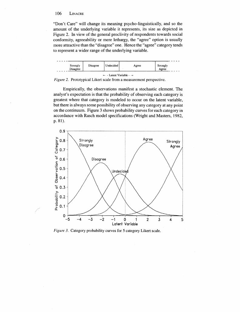
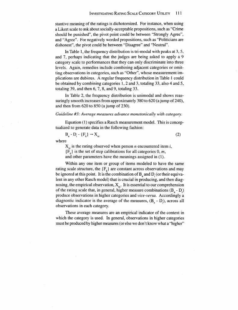