vol. 3, issue 1, january 2014 aquifer parameterization in … parameterization in an alluvial area:...

ISSN: 2319-8753

International Journal of Innovative Research in Science, Engineering and Technology

(An ISO 3297: 2007 Certified Organization)

Vol. 3, Issue 1, January 2014

Copyright to IJIRSET www.ijirset.com 9016

Aquifer Parameterization in an Alluvial Area: Varanasi District, Uttar Pradesh, India- A Case

Study

Poonam Dubey1, M.M.Singh2, H.K.Pandey3

Research Scholar, Institute of Earth Science, Bundelkhand University, Jhansi – 28 41 28, Uttar Pradesh , India1

Associate Professor, Institute of Earth Science, Bundelkhand University, Jhansi – 28 41 28, Uttar Pradesh, India2

Asst. Professor, Motilal Nehru National Institute of Technology, Allahabad - 211004, Uttar Pradesh, India3

Abstract: The principle objective of groundwater study under reference is to estimate the aquifer parameters. Hydraulic properties of aquifers and associated layers have been determined by the pumping test which involves abstraction of water in response to the stress applied due to pumping at a known discharge rate and observing aquifer′s hydraulic head with respect to time. The nature, occurrence and availability of groundwater are directly related to relative thickness of sand and clay zones in the region. Sandy layers form the most significant aquifers in the study area. Good quality potable water is available from coarse grained deep sandy aquifers. On the basis of electrical logging interpretation, the groundwater is saline from ground level to 75.00 m mbgl. The zone from 73.00-78.00 m mbgl has been properly sealed by cement slurry. The well has been shrouded with 3-5 mm pea size gravel up to 75 m from bottom and clay was filled up to the ground surface after proper development. During the well development process by an over-pumping unit, a pumping test was conducted, which comprises of Step Drawdown Test (SDT) and Aquifer Performance Test (APT) to determine the performance, efficiency of well and hydraulic properties of the aquifer respectively. The aquifer parameters evaluated are transmissivity, hydraulic conductivity, storativity, leakage factor, leakance, hydraulic resistance and hydraulic diffusivity. The estimated data shows an appreciable significance regarding the estimation of aquifer properties. As far as the groundwater quality is concerned the groundwater samples collected during SDT is found to be satisfactory, devoid of previous salinity problem which existed earlier.

Key words: Hydraulic properties, Step test, Specific capacity, Transmissivity, Well loss, Well efficiency, Leakance.

I. LITERATURE REVIEW

Indo-Gangetic-Brahmaputra alluvial fill, exceeding 1000 m in thickness at places, constitute the most potential and productive groundwater reservoir in the country. These are characterized by regionally extensive and highly productive multi-aquifer systems (B.M.Jha, S.K. Sinha, 2009)). The correct operation and utilization of boreholes are dependent on the assessment of the productive capacity (yield potential) of the borehole obtained from calculating the storage capacity and the transmissivity of the aquifer (R Owen, T. Dahlin, 2005). According to Kirchner and Van Tonder, the most important information needed to analyze pump test are: information regarding the test hole, depth diameter, water depth level, yield and type of equipment use to test the borehole (Kirchner and Van Tonder, 1991). In addition to usual pumping tests like step test and constant drawdown test, the "calibration test" is sometimes primarily performed to assess the efficiency of the borehole from which the final pumping rate yield for the step test can be determined. On completion of all steps recovery is allowed, preferably exceeding twice the pumping time. Constant discharge test is performed to determine the aquifer

ISSN: 2319-8753





parameter values and to determine the possible existence of groundwater barrier boundaries. It must be emphasis that the calculating done from test pumping data are only representative of the aquifer characteristics in the immediate vicinity of the specific site (R.Owen, T.Dahlin, 2005). Each test must be followed by a recovery period. The aim of whole exercise is to calculate transmissivity, storativity and to determine the sustainable yield. Several methods were developed to analyze and evaluate pump tests (Kruseman and de Ridder 1991). From the drilling logs an appropriate aquifer can be chosen. Knowledge of hydraulic conductivity and transmissivity is essential for the determination of natural water flow through an aquifer (loannis F.louis, George A. Karantonis, Nikolaos S., flippos.louis, 2004) whereas knowledge of geology, boundary conditions, aquifer type, etc. in the neighborhood of the test site is essential as a guide for selecting the correct formula (Bear, 1979). One of the key objectives of well testing is to estimate the amount of water that can be exploited from a well (Misstear and Beeson 2000). Calculation of the total well loss from step drawdown tests provides a meaningful evaluation of well performance. Aquifer transmissivity should be determine in step test from recovery data in the pumped well, not pumping data, to improve accuracy (M.W.Kawecki). Step drawdown tests and its analyses can estimate transmissivity but the estimated value is less accurate than that estimated from a constant rate discharge test. Reduced accuracy is associated with the influence of well design and aquifer characteristics on calculated transmissivity (kruseman and de Ridder 1990). Single-well aquifer tests frequency are analyzed with the Cooper-Jacob method because of its simplicity (Cooper and Jacob1946). Early drawdown data in a pumping well can’t provide reliable estimate of storativity for many reasons. These early data can be used, however to obtain a better estimate of storativity and transmissivity from drawdown data of observation well. The effect of pumping well pipe storage in the early drawdown data may be significant in cases of low transmissivity aquifers and low pumping rates, which are quite common in groundwater remediation (Robert P. Chapuis, 1992).

II. INTRODUCTION

Borehole information reveals that the subsurface lithology is dominated by laterally persistent multi layer of sand capped by thick clayey succession near the top. The nature, occurrence and availability of groundwater are directly related to relative thickness of sandy aquifers. In the western part of Varanasi city, water level is deeper as compared to eastern part of the city. The deep wells penetrating below 60-70 m have enormous yield of 45,000 lph to 220, 50 lph. (Raju N.J., Shukla U.K., Ram P., 2010). Because of thick cover of fine-grained material near the top, these aquifers occur in semi-confined to confined conditions. Differential erosion of the sand horizons by succeeding channel events within a sedimentary package may promote to semi-confined conditions of the aquifers. In general, the ground water of Varanasi city, except nitrate (NO3) all the dissolved solids are within the permissible limit of IS (1991).( Raju N.J., Shukla U.K., Ram P.2010). The drainage system of Varanasi environs is mainly controlled by ′Varuna′ river and ′Assi′ nala. The shallow bore wells (hand pumps) and dug wells puncturing unconfined aquifers at about 25-40 m depth have water-level fluctuations from 3.51 m to 8.25 m. The total thickness of the good water yielding sandy strata varies from 20 to 80 m or more in tube wells occurring at an average depth of about 100 m (CGWB, 2008). A case study of the area shows specific capacity, transsmissivity, storativity and hydraulic conductivity are 228 lpm/m, 7664 m2/day, 212.89 m/day and 278.80 respectively. Recuperation in the observation well obtained within few minutes after shut off the pump indicating that hydraulic conductivity as well as transmissivity is superior. Knowledge of aquifer parameters is essential and important for management of groundwater resources. Conventionally, these parameters are estimated through pumping tests often conducted to obtain aquifer parameters which are necessary information for groundwater studies carried out on water wells. A large number of analytical methods are available for determining aquifer properties from pumping-test data. Different methods have been developed to cope with a wide variety of well and aquifer situations, ranging from simple homogeneous and isotropic aquifers to more complex situations involving anisotropy, boundaries conditions, leaky aquifers, partial well penetration etc. The application of these analytical methods requires both good test data and a good understanding of the assumptions inherent in the methods themselves. An interpretation to hydrological tests can be evaluated both with simple equilibrium approach like using the methods of Hantush and Bierschenk (Bierschenk,1963) and Eden and Hazel (1973) or standard non-equilibrium methods of Jacob

ISSN: 2319-8753





(Cooper and Jacob, 1946) and those of Thies (1935); although both solutions (equilibrium and non-equilibrium) hold several limitation pertaining to field situations. Equilibrium approximations are based on the well known Thiem equilibrium equation (Thiem, 1906). These approximation formulae can be used to provide an initial estimate of aquifer transmissivity in many situations where only limited time drawdown data are available. An estimate of ′T′ from step tests is especially useful in situations where it is not feasible to carry out long constant-rate tests (Misstear and Beeson, 2000). An equilibrium approaches have significant limitations: they cannot be used to determine the aquifer storage coefficient ′S′ and may lead to large errors in estimating ′T′ where equilibrium conditions have not been reached, or have been achieved due to leaky-aquifer conditions or the occurrence of recharge-boundary effects (Misstear, 2001). Though Equilibrium approximation methods such as the Logan formula (Logan, 1964) provide a quick and simple means of deriving an initial estimate of transmissivity in situations where good time-drawdown data are unavailable and methods involving curve matching or fitting straight lines to time-drawdown plots are sometimes misapplied. In practice; to evaluate aquifer parameters : a step-drawdown test (step test /SDT) also referred to as well performance tests, is a single-well pumping test designed to investigate the performance of a pumping well under controlled variable discharge conditions and an aquifer test (APT) of constant-rate discharge test which involves role of observation well in addition. Step tests are applied to determine the yield ′Q′ and efficiency ′E′ of a well. In addition, both methods can be used to determine the nonlinear (turbulent) well loss coefficient ′C′ in Jacob’s well-loss equation (Jacob, 1947) given as:

Sw = B Q + C Q2 where, ′Sw′ is the total drawdown in the pumped well,

′Q′ is the applied pumping rate, and ′B′ is the linear (laminar) head-loss coefficient.

A well loss is directly related to ′Q′ and not to some higher power of ′Q′, one possible cause of linear well loss is a reduction in the permeability at the well face due to clogging of well screen (Mogg, 1969). In a step-drawdown test the pumping rate is increased in a step-wise manner during successive periods of time (Bear, 1979). The step drawdown test is the only test that can result in a functional relationship between drawdown and discharge. Each step is typically of equal duration, lasting from approximately 30 minutes to 2 hours (Kruseman and de Ridder, 1970, 1990) and each step should be of sufficient duration to allow dissipation of wellbore storage effects. The test is recommended to be conducted for at least four steps to ensure accuracy (Clark, 1977). The goal of a step-drawdown test is to evaluate well performance criteria such as well loss ,well efficiency and specific capacity whereas an aquifer test results in quantitative response of an aquifer in terms of transsmissivity, hydraulic conductivity and storativity. Well-performance tests are conducted in order to estimate the energy losses in the aquifer and the pumping well that develop during groundwater extraction. The drawdown in a pumping well consists of the head loss due to the laminar flow as well as the head loss resulting from the turbulent flow of water through the well screens and the pump intake (Batu, 1998). The estimation of these head losses is necessary to evaluate the efficiency, specific capacity and safe yield of pumping wells (Jacob, 1947). The present study focuses on the well and aquifer performance in response to obtain substantial yield with respect to time. A succession of the two tests were conducted, in which data collected at different discharge in ascending order for constant period of time and corresponding drawdown was measured through step test method. Another test, namely aquifer performance test that was carried out after a minimum of 24 hours, the well was pumped at a constant discharge and drawdown (D/D) measured in pumping as well as in observation well. Several factors that can influence discharge quantity and drawdown during pumping are: power pump efficiency, heavy pumping in the vicinity of chosen pumping wells prior to and during a pumping test and the distance between pumping well and observation well (that should not be less than 2b: twice the thickness of aquifer to avoid partial penetration effects) (CGWB, 1982). The method used for discharge measurement is Orifice weir method. This is commonly used to measure the rate of discharge from a turbine pump/submersible pump where the discharge exceeds 500 lpm (Osborne, 1969).

ISSN: 2319-8753





Study area details: The study area selected for pumping test is located at village katharwan, Block Pindra in Varanasi district (Fig.1). It lies in between latitude: 25033′ and longitude: 82049′ (Toposheet: 63k/14).

Fig 1: Location map of the study area

ISSN: 2319-8753





Litholog of Katharawan Exploratory Well, Pindra, Varanasi

Fig. 2: Subsurface lithology through an exploratory well showing litho unit with their corresponding thickness.

III. MATERIALS AND METHODS

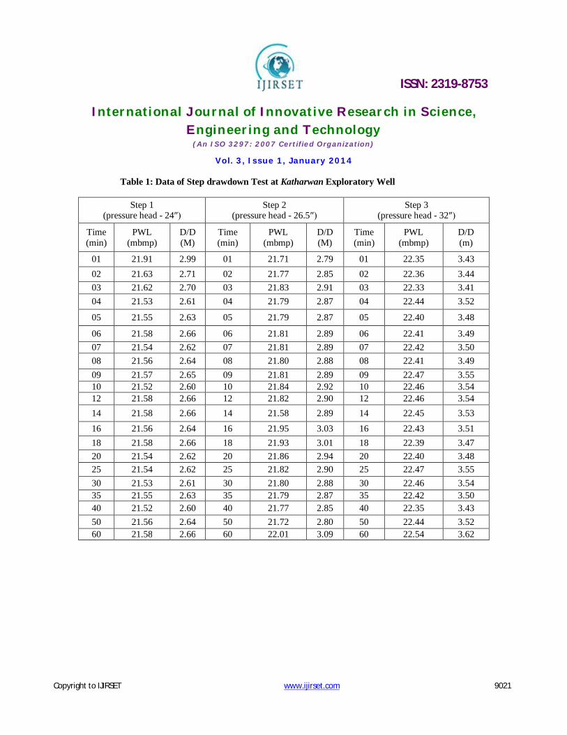
Pumping well and observation well characteristics: The pumping well/Exploratory well (E/W) with diameter 10″/4″ having depth 192 m equipped with 33 m reliable pump and 30 m deep air line assessing the well for water level measurements. Discharge during pumping carried through 10 ft long and 6″ diameter delivery pipe with 4″ diameter Orifice plate. An observation well located 16.60 m away in the periphery of pumping well; to measure the effect of cone of influence during and after pumping process, is 187 m deep with diameter 4″. Step drawdown test (SDT): The present test comprises of three steps of 60 minutes duration. The time -drawdown data so obtained are plotted on semi-log paper and the drawdown curve of each step is extrapolated for 180 minutes (Table 1). Initially static water level measured as 18.42 m mbgl and height of measuring point noted to be 50 cm. Since, the water levels drops very fast in the beginning, the readings were taken at short intervals with gradual increase. The reading on tape at measuring point is noted at a known point (hold); at specified time, the tape is taken out and the reading at the water mark is noted (cut). The difference between the hold and cut gives the water level below the measuring point (mbmp). Only one data point should be selected from each step of the test for use in graphical analysis, except very early points in each step which may be affected by significant changes in well storage (Avci, 1992).

ISSN: 2319-8753





Table 1: Data of Step drawdown Test at Katharwan Exploratory Well

Step 1 (pressure head - 24″)

Step 2 (pressure head - 26.5″)

Step 3 (pressure head - 32″)

Time (min)

PWL (mbmp)

D/D (M)

Time (min)

PWL (mbmp)

D/D (M)

Time (min)

PWL (mbmp)

D/D (m)

01 21.91 2.99 01 21.71 2.79 01 22.35 3.43 02 21.63 2.71 02 21.77 2.85 02 22.36 3.44 03 21.62 2.70 03 21.83 2.91 03 22.33 3.41 04 21.53 2.61 04 21.79 2.87 04 22.44 3.52

05 21.55 2.63 05 21.79 2.87 05 22.40 3.48

06 21.58 2.66 06 21.81 2.89 06 22.41 3.49 07 21.54 2.62 07 21.81 2.89 07 22.42 3.50 08 21.56 2.64 08 21.80 2.88 08 22.41 3.49 09 21.57 2.65 09 21.81 2.89 09 22.47 3.55 10 21.52 2.60 10 21.84 2.92 10 22.46 3.54 12 21.58 2.66 12 21.82 2.90 12 22.46 3.54 14 21.58 2.66 14 21.58 2.89 14 22.45 3.53

16 21.56 2.64 16 21.95 3.03 16 22.43 3.51 18 21.58 2.66 18 21.93 3.01 18 22.39 3.47 20 21.54 2.62 20 21.86 2.94 20 22.40 3.48 25 21.54 2.62 25 21.82 2.90 25 22.47 3.55 30 21.53 2.61 30 21.80 2.88 30 22.46 3.54 35 21.55 2.63 35 21.79 2.87 35 22.42 3.50 40 21.52 2.60 40 21.77 2.85 40 22.35 3.43 50 21.56 2.64 50 21.72 2.80 50 22.44 3.52 60 21.58 2.66 60 22.01 3.09 60 22.54 3.62

ISSN: 2319-8753





Graphical representation of Time vs. Drawdown

Fig.3: Step drawdown test showing the three step process. By increasing discharge rates for each step successively with respect to time; corresponding drawdown was measured which when plotted against increasing time, depicts the gradually falling water levels.

IV. CALCULATIONS

Specific capacity: It is a measure of both the effectiveness of a well and also of the aquifer characteristics (′T′ and ′S′) and simply defines as discharge per unit of drawdown:

C = Q / s, Where, ′Q′ = discharge of the pump in Liters per minute (lpm)

′s′ = drawdown in pumping well after certain time has lapsed. High specific capacities generally indicate a high coefficient of transmissibility, and low specific capacities generally indicate low coefficients of transmissibility. The specific capacity decreases as pumping continues and also with increasing ′Q′. Various authors (Fetter, 2001, Huntley et al. 1992) have established an empirical relationship between the transmissivity ′T′ and the specific capacity ′q′ of the form:

T = C. qa Where, C and a are constants that are empirically determined from available data sets of ′T′ and ′q′. If such a non-linear empirical relationship can be established it may be used as a rough estimate of ′T′ when full aquifer test analysis for a well is not available (Baumle, 2007). But, the specific capacity of a well cannot be an exact criterion of the coefficient of transmissibility because specific capacity is often affected by partial penetration, well loss, and hydrogeologic

ISSN: 2319-8753





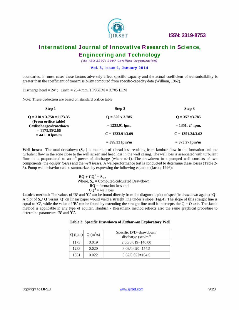
boundaries. In most cases these factors adversely affect specific capacity and the actual coefficient of transmissibility is greater than the coefficient of transmissibility computed from specific-capacity data (William, 1962). Discharge head = 24”; 1inch = 25.4 mm, 1USGPM = 3.785 LPM

Note: These deduction are based on standard orifice table

Step 1

Q = 310 x 3.758 =1173.35 (From orifice table)

C=discharge/drawdown = 1173.35/2.66

= 441.10 lpm/m

Step 2

Q = 326 x 3.785

= 1233.91 lpm,

C = 1233.91/3.09

= 399.32 lpm/m

Step 3

Q = 357 x3.785

= 1351. 24 lpm,

C = 1351.24/3.62

= 373.27 lpm/m

Well losses: The total drawdown (Sw ) is made up of : head loss resulting from laminar flow in the formation and the turbulent flow in the zone close to the well screen and head loss in the well casing. The well loss is associated with turbulent flow, it is proportional to an nth power of discharge (where n>1). The drawdown in a pumped well consists of two components: the aquifer losses and the well losses. A well-performance test is conducted to determine these losses (Table 2-3). Pump well behavior can be summarized by expressing the following equation (Jacob, 1946):

BQ + CQ2 = Sw , Where, Sw = Computed/calculated Drawdown

BQ = formation loss and CQ2 = well loss

Jacob’s method: The values of ′B′ and ′C′ can be found directly from the diagnostic plot of specific drawdown against ′Q′. A plot of Sw/ Q versus ′Q′ on linear paper would yield a straight line under a slope (Fig.4). The slope of this straight line is equal to ′C′, while the value of ′B′ can be found by extending the straight line until it intercepts the Q = O axis. The Jacob method is applicable in any type of aquifer. Hantush - Bierschenk method reflects also the same graphical procedure to determine parameters ′B′ and ′C′.

Table 2: Specific Drawdown of Katharwan Exploratory Well

Q (lpm) Q (m3/s) Specific D/D=drawdown/ discharge (sec/m2)

1173 0.019 2.66/0.019=140.00 1233 0.020 3.09/0.020=154.5

1351 0.022 3.62/0.022=164.5

ISSN: 2319-8753





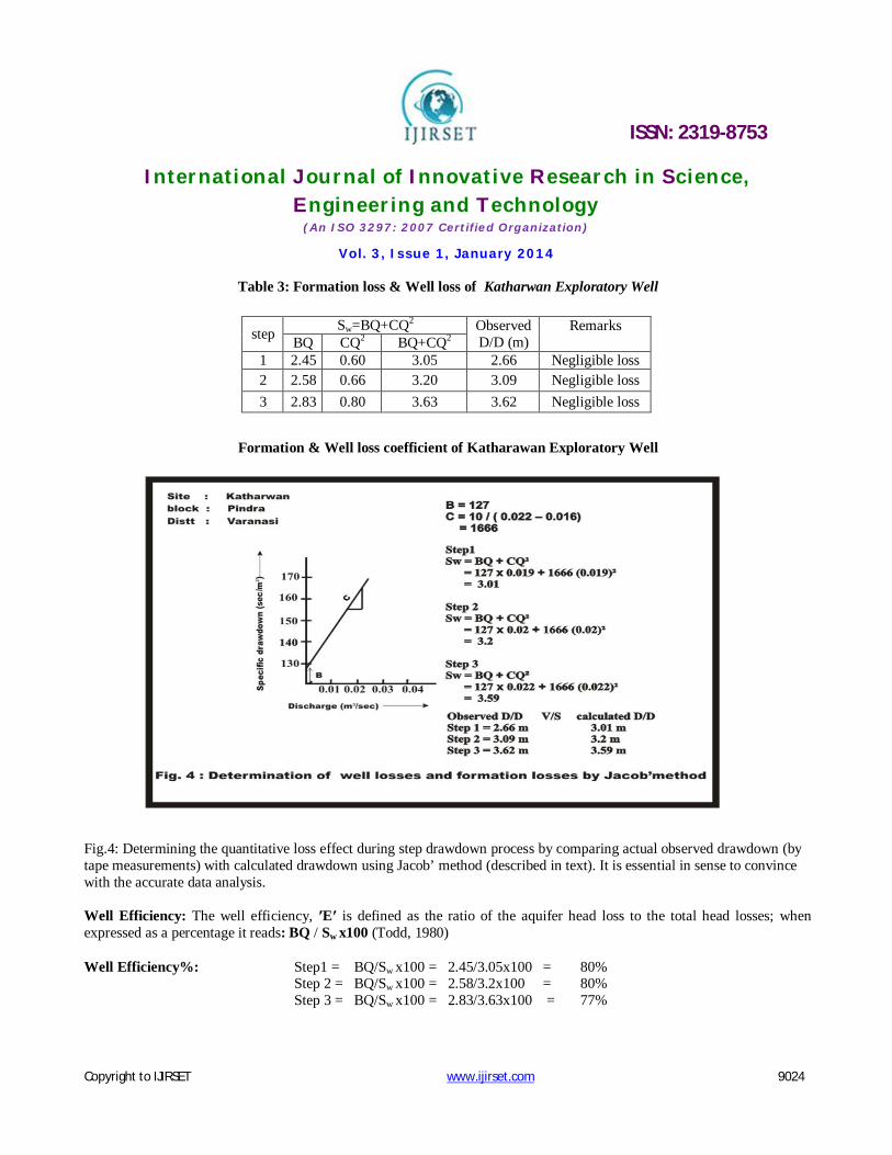
Table 3: Formation loss & Well loss of Katharwan Exploratory Well

Formation & Well loss coefficient of Katharawan Exploratory Well

Fig.4: Determining the quantitative loss effect during step drawdown process by comparing actual observed drawdown (by tape measurements) with calculated drawdown using Jacob’ method (described in text). It is essential in sense to convince with the accurate data analysis. Well Efficiency: The well efficiency, ′E′ is defined as the ratio of the aquifer head loss to the total head losses; when expressed as a percentage it reads: BQ / Sw x100 (Todd, 1980)

Well Efficiency%: Step1 = BQ/Sw x100 = 2.45/3.05x100 = 80% Step 2 = BQ/Sw x100 = 2.58/3.2x100 = 80% Step 3 = BQ/Sw x100 = 2.83/3.63x100 = 77%

step Sw=BQ+CQ2 Observed D/D (m)

Remarks BQ CQ2 BQ+CQ2

1 2.45 0.60 3.05 2.66 Negligible loss 2 2.58 0.66 3.20 3.09 Negligible loss 3 2.83 0.80 3.63 3.62 Negligible loss

ISSN: 2319-8753





Aquifer performance test: During the test, the tube well was made to run at constant discharge of 1397 lpm for 300 minutes with a constant pressure head of 34″. The depressions thus created was monitored with respect to time in both wells (Table 4-5) and plotted on semi-log paper for further analysis. Static water level in both wells measured to be 18.42 m mbgl (E/W) and 18.86 m mbgl (O/W). Distance between both well is 16.60 m. Observation wells can be placed where they will provide the best opportunity to measure the aquifer′s response to the pumping and the boundary effects during the pumping test (King, 1982). Radial distance and location relative to the pumped well; if only one observation well is to be used, is usually located 50 to 300 feet from the pumped well (Osborne, 1969). The data pertaining to the Aquifer Performance (APT) is summarized below:

Table 4: Time vs. Drawdown in Main Well at Katharwan, Pindra, Varanasi

Table 5: Time vs. Drawdown in observation well

Time (min) PWL (mbmp) D/D (m) Time (min) PWL (mbmp) D/D (m) 01 22.33 3.41 30 22.55 3.63 02 22.37 3.45 35 22.51 3.59 03 22.45 3.53 40 22.53 3.61 04 22.48 3.56 45 22.47 3.55 05 22.52 3.60 50 22.56 3.64 06 22.48 3.56 60 22.50 3.58 07 22.56 3.64 70 22.51 3.59 08 22.52 3.60 80 22.54 3.62 09 22.51 3.59 90 22.54 3.62 10 22.50 3.58 100 22.52 3.60 12 22.55 3.63 110 22.48 3.56 14 22.57 3.65 120 22.48 3.56 16 22.58 3.66 140 22.51 3.58 18 22.54 3.62 160 22.52 3.60 20 22.55 3.63 180 22.52 3.60 22 22.52 3.60 200 22.53 3.61 24 22.54 3.62 220 22.60 3.68 26 22.60 3.68 240 22.58 3.66 28 22.59 3.67 300 22.54 3.62

Recovery data Time (min) RWL (mbmp) RD/D (m) Time (min) RWL (mbmp) RD/D (m)

301 18.34 0.58 304 18.20 0.27 302 18.33 0.59 305 18.23 0.69 303 18.32 0.60 306 18.27 0.65

Time (min) PWL (mbmp) D/D (m) Time (min) PWL (mbmp) D/D (m) 0 19.80 0.44 30 19.85 0.49 01 19.80 0.44 35 19.84 0.48 02 19.80 0.44 40 19.84 0.48 03 19.80 0.44 45 19.85 0.49

ISSN: 2319-8753





PWL: Pumping water level, D/D: Drawdown, RWL: Residual Water Level, RD/D: Residual drawdown, Mbmp: Measuring below measuring point

04 19.80 0.44 50 19.84 0.48 05 19.80 0.44 55 19.84 0.48 06 19.79 0.43 60 19.85 0.49 07 19.80 0.44 70 19.85 0.49 08 19.80 0.44 80 19.87 0.51 09 19.80 0.44 90 19.89 0.53 10 19.79 0.43 100 19.86 0.50 12 19.80 0.44 110 19.86 0.50 14 19.80 0.44 120 19.86 0.50 16 19.81 0.45 140 19.86 0.50 18 19.85 0.49 160 19.86 0.50 20 19.84 0.48 180 19.87 0.51 22 19.85 0.49 200 19.86 0.50 24 19.84 0.48 220 19.87 0.51 26 19.84 0.48 240 19.86 0.50 28 19.84 0.48 300 19.86 0.50

Recovery data Time t (min) RWL (mbmp) RD/D (s’) t’ T=300+t’ t/t’

300 19.46 0.1 0 300 0.00 301 19.45 0.09 1 301 301 302 19.44 0.08 2 302 151 303 19.42 0.06 3 303 101 304 19.40 0.04 4 304 76 305 19.40 0.04 5 305 61 306 19.40 0.04 6 306 51 307 19.39 0.03 7 307 43.8 308 19.40 0.04 8 308 38.5 309 19.39 0.03 9 309 34.34 310 19.38 0.02 10 310 31 312 19.38 0.02 12 312 26 314 19.38 0.02 14 314 22.42 316 19.38 0.02 16 316 19.75 318 19.38 0.02 18 318 17.67 320 19.37 0.01 20 320 16 325 19.37 0.01 25 325 13

ISSN: 2319-8753





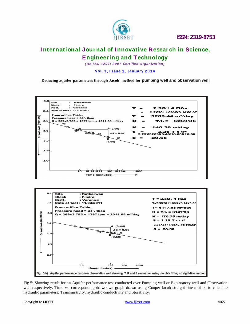
Deducing aquifer parameters through Jacob′ method for pumping well and observation well

Fig.5: Showing result for an Aquifer performance test conducted over Pumping well or Exploratory well and Observation well respectively. Time vs. corresponding drawdown graph drawn using Cooper-Jacob straight line method to calculate hydraulic parameters: Transmissivity, hydraulic conductivity and Storativity.

ISSN: 2319-8753





Recuperation: After completion of pumping process for 300 minutes, the pump made to shut off as to evaluate cone of impression in terms of abruptly rising water levels in observation well (Table 5). Sometimes a pumping well can be influenced by unsuitable efficiency of power pump so that it may be unable to drawn definite yield from an aquifer that results in misinterpretation of data; in this situation an observation well data are more reliable ever. Specifically, recovery tests are easy to perform and provide reliable estimates of transmissivity, (Kawecki, 1995). Recovery tests consist of observing the build-up (or recovery) of hydraulic heads after pumping has stopped. If possible, measurements should continue until the head has recovered to its prior-to-pumping value (Willmann and Carrera, 2007).

Recovery in observation well

Fig.6: When the pumping had stopped; measurement are taken in an observation well to ensure the Transmissivity outcome which reveals in concept of suddenly rising water levels (termed as residual water levels), calculated using Thies’ Recovery

Method.

ISSN: 2319-8753





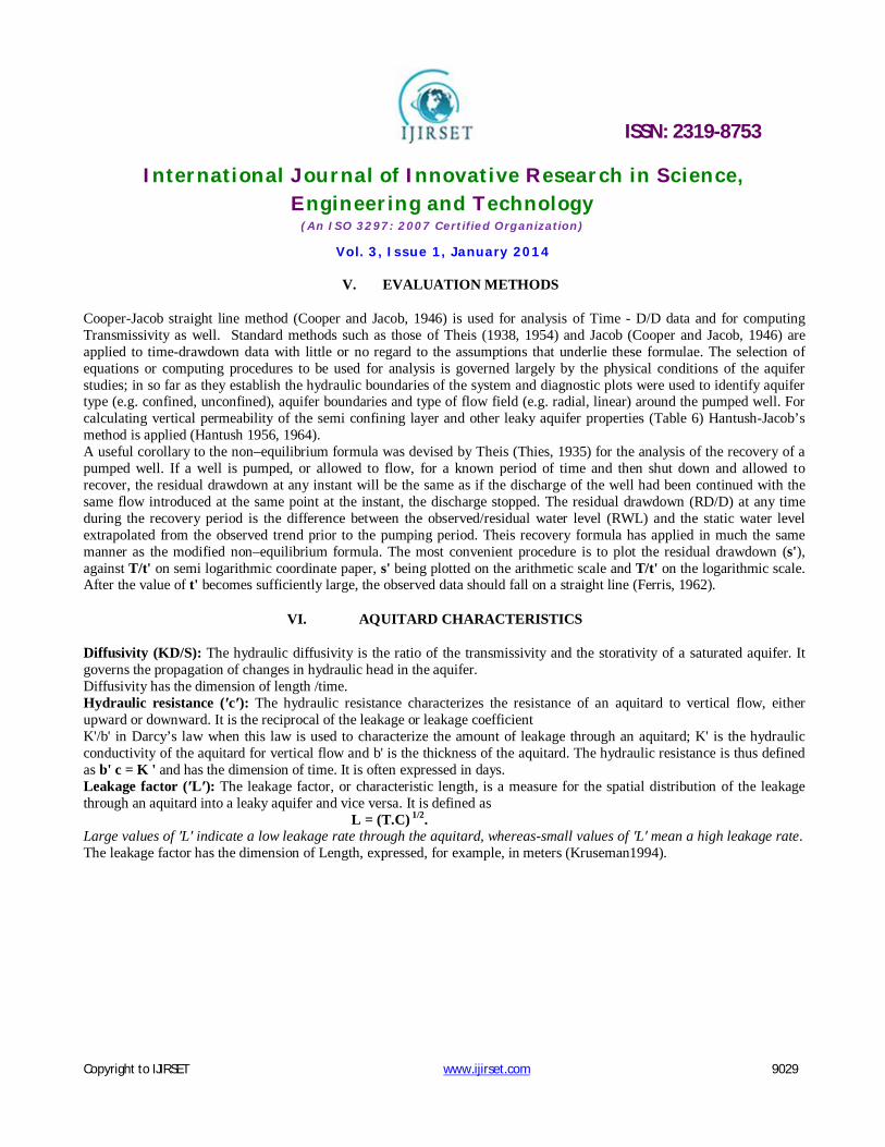
V. EVALUATION METHODS

Cooper-Jacob straight line method (Cooper and Jacob, 1946) is used for analysis of Time - D/D data and for computing Transmissivity as well. Standard methods such as those of Theis (1938, 1954) and Jacob (Cooper and Jacob, 1946) are applied to time-drawdown data with little or no regard to the assumptions that underlie these formulae. The selection of equations or computing procedures to be used for analysis is governed largely by the physical conditions of the aquifer studies; in so far as they establish the hydraulic boundaries of the system and diagnostic plots were used to identify aquifer type (e.g. confined, unconfined), aquifer boundaries and type of flow field (e.g. radial, linear) around the pumped well. For calculating vertical permeability of the semi confining layer and other leaky aquifer properties (Table 6) Hantush-Jacob’s method is applied (Hantush 1956, 1964). A useful corollary to the non–equilibrium formula was devised by Theis (Thies, 1935) for the analysis of the recovery of a pumped well. If a well is pumped, or allowed to flow, for a known period of time and then shut down and allowed to recover, the residual drawdown at any instant will be the same as if the discharge of the well had been continued with the same flow introduced at the same point at the instant, the discharge stopped. The residual drawdown (RD/D) at any time during the recovery period is the difference between the observed/residual water level (RWL) and the static water level extrapolated from the observed trend prior to the pumping period. Theis recovery formula has applied in much the same manner as the modified non–equilibrium formula. The most convenient procedure is to plot the residual drawdown (s'), against T/t' on semi logarithmic coordinate paper, s' being plotted on the arithmetic scale and T/t' on the logarithmic scale. After the value of t' becomes sufficiently large, the observed data should fall on a straight line (Ferris, 1962).

VI. AQUITARD CHARACTERISTICS

Diffusivity (KD/S): The hydraulic diffusivity is the ratio of the transmissivity and the storativity of a saturated aquifer. It governs the propagation of changes in hydraulic head in the aquifer. Diffusivity has the dimension of length /time. Hydraulic resistance (′c′): The hydraulic resistance characterizes the resistance of an aquitard to vertical flow, either upward or downward. It is the reciprocal of the leakage or leakage coefficient K'/b' in Darcy’s law when this law is used to characterize the amount of leakage through an aquitard; K' is the hydraulic conductivity of the aquitard for vertical flow and b' is the thickness of the aquitard. The hydraulic resistance is thus defined as b' c = K ' and has the dimension of time. It is often expressed in days. Leakage factor (′L′): The leakage factor, or characteristic length, is a measure for the spatial distribution of the leakage through an aquitard into a leaky aquifer and vice versa. It is defined as L = (T.C) 1/2. Large values of ′L′ indicate a low leakage rate through the aquitard, whereas-small values of ′L′ mean a high leakage rate. The leakage factor has the dimension of Length, expressed, for example, in meters (Kruseman1994).

ISSN: 2319-8753





Table 6: Properties of leaky aquifer

Hy.diffusivity ′D′ (m2/day) D = T/S

Leakance 1/C (/day) 1/C = K’/b’

Hy.Resistance ′C′ (time unit) C = b’/K’

Leakage factor ′L′ (m2) L= (T.C)1/2

276.98 4.40 0.22 161.08

Table 7: Step wise result of Aquifer under SDT

Table 8: Aquifer Parameters under Aquifer Performance Test

VII. RESULTS AND DISCUSSIONS

Step drawdown test: (Fig 3). The first few points reflect the effect of well storage (Segment 1). Segment 2, indicates the effect of contribution from aquifer in the form of inflow (in pumping well during pumping). The third segment which also falls on a straight line indicate: a gentler slope as compared with segment 2 indicating an increase in aquifer Contribution ('q') as compared to the pump discharge ′Q′, often leading to a steady state condition. Sometimes the slope of the segment 3 steepens as compared with segment 2. This indicates the limited extent of the aquifer, showing sudden increase in the rate of drawdown (i.e. Aquifer contribution ′q′ is much smaller than the pump discharge ′Q′). A smooth curve obtained from SDT data falls on a nearly straight line, indicates that there are rapid increases in the drawdown with respect to increasing discharge rate. In response to pumping, the confined, semi-confined and semi-unconfined aquifers behave differently. The distribution head in response to pumping depends on the degree and extent of insulation of the aquifer. In case of specific capacity which decreases with the period of pumping (Table 9) due to the fact that the drawdown continually increases with time as the cone of influence of the well expands. Hence, duration of the pumping period for which a particular value of specific capacity is computed, is important. Exploratory wells of sp.capacity 250 lpm/m drawdown and above falls under category ′A′ for alluvial areas. The specific capacity of the well works out to be 404 lpm/m; therefore it falls under this category (Table 9). The pumping well is liberated from loss effects and remarked to be negligible due to the reason that observed drawdown and calculated drawdown are similar (Table 3, Fig.4), as a consequence to this well efficiency is also good enough.

Step Pumping duration

(min)

Discharge (lpm)

Max D/D (m)

Sp.capacity (lpm/m)

Well efficiency

(%) Category of well

1 60 1173 2.66 441.10 80 A 2 60 1233 3.09 399.32 80 A 3 60 1351 3.62 373.27 77 A

S.no. Method Well data T (m2/day) S K (m/day) Sp.capacity (lpm/m)

1 Jacob 1) O/W 2) E/W

1) 6147.68 2) 5269.44

1) 20.58 2) 20.65

1) 170.75 2) 146.36

1) E/w- 385.9 2) O/W- 2794

2 Theis Recovery O/W 7377 - - - 3 Average value O/w & E/w 5708.56 20.61 158.55 1589.95

ISSN: 2319-8753





Aquifer Performance Test: An average of transmissivity, hydraulic conductivity and storativity in the region estimated are 5708.56 m2/day, 158.55 m/day and 20.61 respectively. Cone of influence expends up to 16.60 m. Drawdown levels are influenced by vertical leakance of 4.40 lpd/m3 through aquitard during pumping. Over all data collected for evaluation of aquifer parameters are good and accurate due to the fact that plots give numerical values appropriate in all aspects, even fitting a straight line for computing ′T′ is absolutely effortless (Fig.5 a, b). Recovery graph shows a straight line representing rapid rising water level due to high value of transmissivity rate of the aquifer (Fig. 6).

VIII. CONCLUSIONS

Based on litho log (Fig. 2) analysis and transmissivity value estimated; the aquifer tapped is semi-confined in nature (T ranges 4500 m2/day to 10000 m2/day for semi-confined aquifers), since sand horizons are overlain by the clay/silt layers through which vertical leakage takes place due to head difference. A steady-state flow condition found at the end of the pumping (steady state is attained when the time-drawdown curves become straight-horizontal lines). There is no considerable effect of partial penetration of aquifer on yield and transmissivity of aquifer.

Recuperation obtained immediately after shutting down of pump and took only 20-30 minutes for its full recuperation. Hence, the aquifer has good transmissivity and it obtained almost full recovery. Recovery data does not involve the effect of well storage on pump discharge (as the pump is shut off) and contains the effect of the contribution of water from the aquifer only. Transmissivity values obtained from both well vary to a small extent as pumping wells always affected due to fluctuations during pumping rather than observation well which gives definite value of transmissivity and hydraulic conductivity in an area particularly during recovery.

After a period of 300 min, when the pump has been shut down the water level in the well (especially in observation well) started to rise so rapidly. In this condition the water from the surrounding aquifer continue to flow towards the well under the influence of the hydraulic gradient. Due to rise in water level the hydraulic gradient towards pumping well becomes gentler with time, thereby reducing the rate of the aquifer contribution ′q′. Now, the water required for this re-saturation process is derived by dewatering the peripheral areas of cone of depression i.e. cone of depression continues to expand in peripheral areas even after the pump is switched off. Slowly, with time, the water level rises in the well and finally gets stabilized at a new static water level which may be fractionally lower as compared to the original static water level. Acknowledgement: This work reflects a section of dissertation work carried out by author. The author is highly grateful to the Central Groundwater Board, Ministry of water resources, Government of India for providing the logistic support and guidance.

ISSN: 2319-8753





REFERENCES

[1] Avci C.B., "Parameter estimation for step-drawdown tests", Ground Water J, 30(3):338–342, 1992 [2] B.M. Jhha, S.K. Sinha,"Towards better management of ground water resourses of India, report CGWB, 2009 [3] Batu V., "Aquifer hydraulics: a comprehensive guide to hydrogeologic data analysis", Wiley, New York, 727 pp, 1998 [4] Bäumle R., Neukum Ch., Nkhoma J., Silembo O., "The groundwater resources of Southern Province, Zambia"- Ministry of Energy and Water

Development – Department of Water Affairs, Zambia & BGR – Federal Institute for Geosciences and Natural Resources, Germany; Phase 1 Technical Report Vol. 1(Nov. 2007); 132 pages; Lusaka., 2007

[5] Bear J., "Hydraulics of groundwater", Mc-Graw hill, 569pp, 1979 [6] Bierschenk W.H., "Determining well efficiency by multiple step-drawdown tests"- International Association of Scientific Hydrology, Publication

64: 493-507, 1963. [7] CGWB, " A technical report on Groundwater Scenario of Varanasi district and its Management, Ministrey of Water Resourses, Government of

India", 2008 [8] CGWB, " Manual-Evaluation of Aquifer Parameters, Central Groundwater Board. Ministry of Irrigation, Government of India", 1982 [9] Clark L., "The analysis and planning of step-drawdown tests", Hydrogeol J Eng Geol Q, 10(2):125–143, 1977 [10] Cooper H.H.J, Jacob C.E., "A generalized graphical method for evaluating formation constants and summarizing well field history", Trans Am

Geophys Union 27:526–534, 1946 [11] Eden R.N., Hazel C.P., "Computer and graphical analysis of variable discharge pumping tests of wells", Civil Eng Trans J,15 (1–2):5–10, 1973 [12] Ferris J. G., Knowles, D. B., Brown, R. H. and Stallman, R. W., "Theory of Aquifer Test", U.S. Geological Survey Water Supply Paper 1536-E,

pp 69-174, 1962 [13] Fetter C. W., "Applied Hydrogeolgy"- 4th ed. 598 pages; Prentice Hall; Upper Saddle River, New Jersey, 2001 [14] Hantush M.S. , "Analysis of data from pumping tests in leaky aquifers". Traps Am. Geophys. Union 37 702-714, Ground Water J, 33(1):23–32,

1965 [15] Hantush M.S. , "Hydraulics of well, Advances in hydrosciences" ed. V.T. Chow Vol.1 Academic press, New York and London, 1964(a) [16] Hantush M.S., "Aquifer tests on partially penetrating wells", Hydrogeol J,. Div., Proc. of the Am. Soc. of Civil Eng., vol. 87, no. HY5, pp. 171-

194, 1961(b) [17] Huntley D., Razack, M .," Assessing transmissivity from specific capacity in a large and heterogeneous alluvial aquifer", Ground Water J,

29(6):856–861, 1991 [18] Jacob C. E., "Drawdown test to determine effective radius of artesian well."-Trans. American Society of Civil Engineers 112, Paper 2321: 1047-

1064, 1947 [19] Kawecki M.W., " Meaningful interpretation of step-drawdown tests", Hydrogeol J, vol.33, no.1-Groundwater, 1995 [20] King H. W., "Handbook of Hydraulics", McGraw-Hill Book Co., New York, 1982. [21] Kirchner J., van Tonder G.J. and Lucas E., "Exploitation potential of Karoo aquifers", WRC Report 170/1/91, Water Research Commission,

Pretoria, 1991 [22] Kruseman G.P, de Ridder N.A., "Analysis and evaluation of pumping test data", 2nd edn. Publ 47(ILRI), Wageningen , ISBN 90-70754-20-7,

1990 [23] Kruseman G.P., "Analysis and Evaluation of Pumping Test Data", Intl. Inst. for Land Reclamation and Improvement, Bull.11, Nageningen, 1970 [24] Kruseman, G.P. and de Ridder N.A., "Analysis and evaluation of pumping test data", International Institute for Land Reclamation and

Improvement, Wageningen, The Netherlands, pub. 47, 377 pp, 1991 [25] Loannis F. Louis, George A. Karantonis, Nikolaos S. Voulgaris and Flippos I.Louis."The contribution of geophysical methods in the

determination of aquifer parameters: The case of Mornos River Delta,Greece",Res.J.Chem.Environ,vol.8(4), Dec 2004. [26] Logan J., "Estimating transmissibility from routine production tests of water wells", Ground Water J, 2:35–37, 1964 [27] Misstear and Bruce D.R., "The value of simple equilibrium approximations for analyzing pumping test data", Associate Editor Hydrogeol J,

(2001) 9:125–126, 2001 [28] Misstear BDR, Beeson S., "Using operational data to estimate the reliable yields of water-supply wells", Hydrogeology J, 8:177–187, 2000 [29] Mogg j.L., "Step drawdown tests need critical review", Groundwater J, v.7 no.1, pp28-34,1969 [30] Osborne Paul S., " EPA groundwater issue, suggested operating procedures for aquifer pumping test", 1969 [31] R.Owen, T.Dahlin, "Alluvial aquifer at geological boundaries: Geophysical investigation and groundwater resourses" chapt 19: lup.lub.

lu.se/record/2344532, 2005 [32] Raju N.J., Shukla U.K., Ram P. , "Hydrogeochemistry for the assessment of groundwater quality in Varanasi: a fast –urbanizing centre in Uttar

Pradesh, India" , 2010

ISSN: 2319-8753





[33] Robert P.Chapuis, "Using Cooper-Jacob approximation to take account of pumping pipe storage effects in early drawdown of a confined aquifer", 1992

[34] Theis C. V., "The significance and nature of the cone of depression in ground-water bodies", Economic Geol J, v. 33(8), 1938 [35] Theis C.V. and Brown R. H., "Drawdown in wells responding to cyclic pumping" U.S.Geol. Survey, Groundwater Note 23, 1954 [36] Theis C.V., "The relation between the lowering of the piezometric surface and the rate and duration of discharge of a well using groundwater

storage", Trans Am Geophys Union 16:519–524, 1935 [37] Thiem, G., "Hydrologische methoden". Gebhardt, Leipzig, 1906. [38] Todd D.K., "Groundwater Hydrology" , Jhon wiley NewYork 2nd edition, 1980 [39] William C. Ackermann , "Using operational data to estimate the reliable yields of water-supply wells, State water survey division, Chief

URBANA" . Hydrogeol J., 8:177–187, 1962 [40] Willmann M., Carrera, J., Sánchez-Vila, X., Vázquez-Suñé, E., "On the meaning of the transmissivity values obtained from recovery tests",

Hydrogeol J., Springer-Verlag 200. 15: 833–842, 2007 [41] Wu YS., "An approximate solution for non-Darcy flow toward a well in fractured media", Water Resour Res 38:10.1029, 2002

vol. 3, issue 1, january 2014 aquifer parameterization in … parameterization in an alluvial area:...

Documents