UIC Intermediate Progress Report

REU 2004 Summer Program

VOC Reduction by Dynamic Condenser Design

Student’s Name: Melanie Rondot Advisors: Professor Andreas Linninger

Andrés Malcolm, graduate student

Laboratory for Product and Process Design University of Illinois at Chicago

LPPD-Project Report: 08/05/2004

1

ABSTRACT

Organic solvents used in pharmaceutical manufacturing operations are volatile;

thus, the vapor in equilibrium with the solvents contains species known as Volatile

Organic Compounds (VOCs). The release of VOCs to the atmosphere is hazardous to the

public health and is regulated by the EPA. Surface condensation is the preferred method

for the reduction of VOCs in an emissions stream.5

A mathematical model has been developed to simulate the operation of a surface

condenser. It is based on the principle of diffusion-controlled condensation, which states

that condensation will occur if the concentration gradient between the bulk gas and the

gas-condensate interface promotes diffusion of the condensable species toward the

interface and the vapor is saturated at the wall temperature. The model has been designed

for a shell-and-tube condenser, where it is assumed that the condensate is removed from

the condenser as it is formed, leaving only a thin film of liquid on outside walls of the

coolant tubes. The thickness of this film is constant and its temperature is assumed to be

equal to the wall temperature. The model uses finite volume discretization across the

length of the condenser to form a system of equations (mass balances, energy balances,

and diffusion equations) which must be solved simultaneously. These computations are

performed using MATLAB. The algorithm outputs the temperature, concentration, and

flow profiles along the length of the condenser for steady state operation. Output from the

dynamic model traces the temperature change of a specified volume element with time,

as well as the changes in flowrate of condensate, concentration in the bulk gas, and

concentration near the wall.

Limitations on the validity of the diffusion-controlled condensation model were

discovered. The model was updated to include the situation where the temperature of the

bulk gas reaches the wall temperature and condensation occurs in the bulk phase without

diffusion to the wall (i.e. heat transfer controlled condensation). The heat transfer

limitation was imposed to ensure a physically valid solution; however, the change in fluid

dynamics resulting from condensation in the bulk phase was not considered. Thus, the

model should be used only in situations where diffusion-controlled condensation occurs.

The effect of uncertainty in system parameters has been analyzed, thus indicating

which factors must be considered when designing a condenser to treat an inlet stream

2

according to EPA regulations. A dynamic controller has been implemented in order to

improve the efficiency and minimize the cost of the process. The controller minimizes the

error between the outlet gas temperature and the desired set point by adjusting a system

variable such as the coolant flowrate.

3

TABLE OF CONTENTS ABSTRACT............................................................................................................................................1 INTRODUCTION...................................................................................................................................4

Motivation...........................................................................................................................................4 Approach.............................................................................................................................................6 Outline ................................................................................................................................................6

METHODOLOGY..................................................................................................................................7 Process Description.............................................................................................................................7 VOC Emission Calculations ...............................................................................................................8 Condenser Theory...............................................................................................................................9 Condenser Model..............................................................................................................................14

System Variable Calculations ......................................................................................................14 Steady State Model.......................................................................................................................15 Dynamic Model............................................................................................................................17

Uncertainty Evaluation .....................................................................................................................18 Control System .................................................................................................................................19

RESULTS AND DISCUSSION............................................................................................................25 Steady State Uncertainty Evaluation ................................................................................................25

Independent Variation of One Variable (Cpgas, hgas, Dab change with position)......................26 Simultaneous Variation of Two Variables (Cpgas, hgas, Dab change with position)..................29

Design Applications..........................................................................................................................33 Model Robustness.............................................................................................................................34

CONCLUSIONS...................................................................................................................................37 FUTURE WORK ..................................................................................................................................37 ACKNOWLEDGEMENTS ..................................................................................................................38 REFERENCES......................................................................................................................................39 APPENDIX I: Regulations for VOC Emissions by Pharmaceutical Manufacturing Facilities in Chicago, Illinois 7 ..................................................................................................................................41 APPENDIX II: Calculation of VOC Emissions 10 ................................................................................42 APPENDIX III: Derivation of Diffusion Equation from Fick’s Law 12................................................44 APPENDIX IV: System Variable Calculations and Correlations .........................................................45 APPENDIX V: Condenser Model - MATLAB Program Code.............................................................47

Dynamic Model ................................................................................................................................47 Main Program...............................................................................................................................47 Steady State Solution ...................................................................................................................53 Steady State Plot...........................................................................................................................55 Dynamic Solution.........................................................................................................................56 Dynamic Plot 1.............................................................................................................................59 Dynamic Plot 2.............................................................................................................................60

Control Model...................................................................................................................................61 Main Program...............................................................................................................................61 Steady State Solution ...................................................................................................................66 Steady State Plot...........................................................................................................................67 Dynamic Solution.........................................................................................................................68 Dynamic Plot 1.............................................................................................................................70 Dynamic Plot 2.............................................................................................................................70 Dynamic Controller Plot ..............................................................................................................70

APPENDIX VI: Steady State Uncertainty Evaluation ..........................................................................71 Independent Variation of One Variable (Cpgas, hgas, Dab constant) ..............................................71 Independent Variation of One Variable (Cpgas, hgas, Dab change with position) ..........................72 Simultaneous Variation of Two Variables (Cpgas, hgas, Dab change with position) ......................73

4

INTRODUCTION

Motivation

Typical pharmaceutical processes involve the use of organic solvents, both within

the reaction and separation steps and the cleaning of vessels after a reaction has occurred

(see Figure 1). These organic solvents often have low vapor pressures, giving rise to

volatile organic compounds (VOCs) in equilibrium with the liquid solvent. The emission

of VOCs into the atmosphere is hazardous to the public health. In the presence of

ultraviolet light, VOCs react with nitrogen oxides in the atmosphere to form tropospheric

ozone, the primary component of smog.1 In the Clean Air Act Amendments of 1990, the

Environmental Protection Agency (EPA) established regulations for VOC emissions.2

Individual states have developed their own procedures in order to comply with the EPA

regulations. These state implementation plans can be found on the EPA’s website.3

Many different methods exist for reducing the VOC concentration in a vapor

stream. Although procedures such as combustion, adsorption, and absorption (scrubbing)

are available, they possess inherent disadvantages which make surface condensation the

preferred approach. Complete combustion of VOCs results in the formation of carbon

dioxide and water. However, the efficiency and rate of combustion are dependent on the

Figure 1: Flow Diagram for Typical Pharmaceutical Process4

5

residence time, temperature, and turbulence of the stream. For variable flowrates, the

process becomes difficult to control and may result in incomplete combustion and the

release of undesirable products into the atmosphere. Adsorption onto a catalyst bed is

another technique used for removing VOCs from a vapor stream. However, when a bed

becomes saturated, it must be regenerated before being returned to service. Regeneration

involves desorbing the adsorbed gases, usually by heating or applying a vacuum, and

results in an air stream which contains the original VOCs. In absorption, or scrubbing,

components from the vapor stream are dissolved in a liquid solvent. This procedure is

sensitive to the solubility of the VOC in the selected solvent and must be followed by a

process to recover the VOC from the solvent.5 Condensation can be achieved by either

lowering the system temperature or increasing the pressure. Components with lower

vapor pressures will condense first, thus allowing for the separation of mixtures. In

surface condensation, there is no contact between the vapor stream and the coolant. The

VOCs condense on the outside walls of the coolant tubes and, since they have not been

contaminated by the coolant, solvents can be recovered from the condensate and

recycled.6

The EPA has recognized the desirability of using surface condensers to reduce

VOC emissions. Based on the vapor pressure of the VOC in the inlet stream, the EPA has

specified acceptable temperatures for the gas leaving a condenser. Other types of air

pollution equipment are merely governed by a required percent reduction in VOC

emissions.7 Regulations for VOC emissions by pharmaceutical manufacturing facilities in

Chicago, Illinois can be found in Appendix I.

The regulation of VOC emissions must be considered from an economic as well

as environmental standpoint. Although VOC reduction is a necessary operation, it is a

costly addition to a manufacturing process. In addition to the capital cost of the

equipment, companies are also faced with operating costs such as materials, utilities, and

labor. The cost of reducing VOC emissions must be weighed against the cost of

generating VOC emissions. In an emissions treaty scheme, companies must purchase

permits which allow them to emit a specific amount of VOCs during a set period of time.

In the Chicago area, an allotment trading unit (ATU) represents 200 pounds of VOC

emissions during the seasonal allotment period, which extends from May 1 to September

6

30. The allotment period is followed by a reconciliation period (October 1 to December

31) in which companies compile emissions data and submit an annual emissions report to

the EPA. Companies must possess a sufficient amount of ATUs by the end of the

reconciliation period to cover their actual emissions from the preceding season.8

The economic incentive to reduce both VOC emissions and operating costs leads

to a design optimization problem. By implementing a dynamic control system,

parameters such as the coolant flowrate can be adjusted as the inlet conditions change.

Thus, the desired separation can be obtained at a minimum operating cost.

Approach

In order to optimize the design of a condenser, a thorough understanding of its

operation is required. For this purpose, a mathematical model based on diffusion-

controlled condensation was developed and was solved using MATLAB. Based on user-

specified initial conditions and physical properties, the program computes the required

heat and mass transfer variables and simulates the operation of the condenser by solving

the system of mass and energy balances. The performance of the model was evaluated

through trials using various initial conditions and modifications were made as necessary.

The model is used as a basis for developing a dynamic control system for the operation of

a condenser. The control system will reduce the cost associated with VOC emissions by

allowing the process to continuously operate at the optimal balance between reduced

operating cost and increased performance. The model has also been used to analyze the

impact of uncertainty on the operation of the condenser.

Outline

The remainder of this paper is organized as follows. Typical operations in which

VOCs are generated are described in the process description, followed by an explanation

of how a surface condenser can be used to reduce the concentration of a VOC in a vapor

stream. Next, the procedure for calculating the amount of VOC generated in an operation

is outlined. The theory behind the operation of a condenser (including mass and energy

balances and diffusion-controlled condensation) is presented before explaining the details

of the mathematical model which has been developed. The dynamic control system for

7

the condenser is described and the procedure for evaluating the effect of uncertainty is

given. Information on VOC emission regulations is contained in Appendix I, while

Appendix II shows the method for calculating VOC emissions. The derivation of the

diffusion equation is given in Appendix III. The correlations used for estimating system

parameters are detailed in Appendix IV. Appendix V contains program code, and the

results of the uncertainty evaluation are shown in Appendix VI.

METHODOLOGY

Process Description

As shown in Figure 1, organic solvent vapors are generated at various stages

throughout the manufacture of a pharmaceutical product. This project focuses on the

VOCs formed in the reactor and their treatment in the condenser located immediately

after the reactor.

The use of organic solvents in the reaction itself, the subsequent separation steps,

and the cleaning process used to prepare the vessel for future operations results in the

formation of VOCs. After these operations, the tank is purged with nitrogen in order to

displace the air present in the vessel. At temperatures low enough to condense the VOCs,

moisture in the air would freeze inside the condenser and result in decreased

performance.2 The presence of an inert such as nitrogen also prevents the vapor from

becoming flammable.9

The case studies used to evaluate the condenser model focused on the operation of

charging a vessel with ethanol, followed by a nitrogen sweep. A diagram of the procedure

is shown in Figure 2. After the charge and sweep operations, the used solvent is

discharged from the reactor as a liquid. The vapor stream consists of the solvent vapors

(VOCs) and nitrogen. The vapor stream is passed through a condenser, with its flow to

the condenser being controlled by a valve. A shell-and-tube condenser is used for the

separation. The vapor passes through the outer shell while the coolant flows through

tubes contained within the interior of the shell. The condensate forms on the outer wall of

the tubes. Both the condensate and the vapor containing nitrogen and uncondensed VOC

exit from the shell of the condenser. A cryogenic coolant is used to efficiently achieve the

low temperatures required for condensation of the VOCs.

8

Figure 2: Process Flow Diagram for Reactor-Valve-Condenser System

VOC Emission Calculations

In order to determine the applicability of EPA regulations to a given operation,

the VOC emissions must be calculated. EPA Publication 290580: “Control of Volatile

Organic Emissions from Manufacture of Synthesized Pharmaceutical Products”10 outlines

the methods for calculating emissions from the following operations:

- Charging

- Evacuation (Depressurizing)

- Nitrogen or Air Sweep

- Heating

- Gas Evolution

- Vacuum Distillation

- Drying

Calculations involving the charging of a vessel with ethanol followed by a nitrogen

sweep can be found in Appendix II.

Another method for determining the VOC concentration in a process stream is to

perform a computer simulation of the process. The program Batch Design Kit (BDK) was

used to simulate the charge and sweep operations and the results were compared to those

calculated according to the EPA documentation.

9

Condenser Theory

Figure 3 shows a two-dimensional view of a typical shell and tube condenser. The

vapor stream flows through the outer shell while the coolant passes through the inner

tube. (Multiple coolant tubes are usually used to improve efficiency.) The condensate is

removed at various points along the length of the condenser. By using a finite volume

discretization along the length of the condenser (see Figure 4), the applicable mass and

energy balances form a system of differential and algebraic equations. The condenser

model uses MATLAB to solve this system of equations and obtain flow, temperature, and

concentration profiles along the length of the condenser.

Figure 3: Diagram of Co-current Condenser11 Gas stream flows through outer shell of condenser while coolant passes through inner tube. Components from gas stream condense on outer surface of coolant tubes. Condensate is removed from the shell as it forms.

Figure 4: Example of Finite Volume Discretization of a Condenser11

Flow of coolant, gas, and condensate streams entering and exiting each element is considered. Energy transfer between wall and coolant and wall and gas is also considered for each volume element.

Gas Inlet

Gas Outlet

Coolant Inlet

Coolant Outlet

Condensate Outlets

Gas Inlet

Gas Outlet

Coolant Inlet

Coolant Outlet

Condensate Outlets

Wall T wall

1

Coolant T cool 1 , N cool

Gas T g 1 ,Ng 1

Condensate F co 1 ,T co 1

F cool ,T cool 0 F cool ,T cool 1

q w - cool 1

F g 0 ,T g 0 F g 1 ,T g 1

q w - g 1 Wall T wall

2

Coolant T cool 2 , N cool

Gas T g 2 ,N g 2

Condensate F co 2,T co 2

F cool ,T cool 2

F g 2 ,T g 2

Wall T wall

3

Coolant T cool 3 , N cool

Gas T g 3 ,Ng 3

Condensate F co 3 ,T co 3

F cool ,T cool 3

F g3 ,T g 3

q w - cool 3 q w- cool 2

q w - g 2 q w - g 3

10

The underlying assumption of the model is that condensation is diffusion

controlled. When the concentration of VOC in the vapor stream is greater than the

concentration of VOC near the tube wall (due to the vapor pressure of the VOC in

equilibrium with the condensate), diffusion of the VOC from the bulk gas to the gas-

condensate interface will occur. When the VOC molecules reach the gas-condensate

interface, the temperature of the condensate is sufficiently low for condensation of the

vapor to occur. It is assumed that the condensate is removed from the condenser as it is

formed, leaving only a thin film of liquid on the tube wall. The thickness of this film is

constant and its temperature is equal to the wall temperature.

Figure 5 shows the temperature and concentration profiles within a finite volume

element of the condenser. The temperature and concentration of the bulk gas are constant.

Within the gas boundary layer, the temperature and concentration of the gas change

gradually until the conditions at the gas-condensate interface (as specified by vapor-

liquid equilibrium) are reached. The condensate film consists solely of the condensable

component of the gas, and its temperature is equal to the wall temperature. The coolant

temperature changes from the wall temperature to that of the bulk phase throughout the

coolant boundary layer.

Gas

����������������������������������������������������������������������������������������������������������������������������������������������������������������������������������������������������������������������������������������������������������������������������������������������������������������������������������������������������������������

Wal

l

Cond

ensa

te F

ilm

Gas

Bou

ndar

y La

yer

PC,Condensable

PNC,Non-Condensable

Tg,Gas Mixture

TI

PSNC(TI)

Twall

PSC(TI)

Cool

ant

Cool

ant B

ound

ary

Laye

r

Tcool,Coolant

Gas

����������������������������������������������������������������������������������������������������������������������������������������������������������������������������������������������������������������������������������������������������������������������������������������������������������������������������������������������������������������

Wal

l

Cond

ensa

te F

ilm

Gas

Bou

ndar

y La

yer

PC,Condensable

PNC,Non-Condensable

Tg,Gas Mixture

TI

PSNC(TI)

Twall

PSC(TI)

Cool

ant

Cool

ant B

ound

ary

Laye

r

Tcool,Coolant

Figure 5: Temperature and Concentration Profiles in a Finite Volume Element11

In the gas boundary layer, the gas temperature decreases from that of the bulk phase to that of the wall and condensate film. The concentrations of condensable and noncondensable species in the gas (designated as partial pressures) also change as prescribed by vapor-liquid equilibrium between the gas phase and the condensate. The temperature change of the coolant occurs in the coolant boundary layer rather than the bulk phase. The temperature and concentration gradients occur perpendicular to the direction of fluid flow through the element.

11

In order to obtain the system of equations describing the condenser, energy and

mass balances must be performed on each finite volume element:11

Energy Balances

Equation (1a) shows the energy balance for the gas phase: the change in energy of the gas

phase is equal to the change in enthalpy between the inlet and outlet gas streams minus

the enthalpy of the condensate and the energy transferred to the wall. Equations (1b),

(1c), and (1d) manipulate equation (1a) to obtain a simplified form.

1 1( . ). . . . . . .

n ng g n n n n n n n

pg g pg g g pg g condensate pg w w g

d N TC F C T F C T F C T Q

dt− −

−= − − − (1a)

1 1( ) ( ). . . . . .

n ng gn n n n n n n n n

pg g g g pg g g pg g condensate pg w w g

d T d NC N T F C T F C T F C T Q

dt dt− −

−

+ = − − −

(1b)

1( )ngn n n n

pg g g g g

d TC N T F F

dt−+ −( ) 1 1. .n n n n n

condensate g pg g g pg gF F C T F C T− − − = −

.n n ncondensate pg w w gF C T Q −− − (1c)

1 1. . .( ) . .( )n

gn n n n n n n ng pg g pg g g condensate pg g w w g

dTN C F C T T F C T T Q

dt− −

−= − + − − (1d)

Equation (2) shows that the energy transferred to the wall from the gas phase is equal to

the energy obtained from the cooling and condensation of the gas plus the heat

convection from the gas phase to the gas-wall interface.

( ). .( ) ( )n n n n n v nw g g condensate pg g w g wQ Q F C T T H T− = + − + ∆ (2)

Equation (3) calculates the heat convection from the gas to the gas-wall interface.

.( )n n ng g g wQ T Tα= − (3)

Equation (4) shows the energy balance for the coolant: the change in energy of the

coolant is equal to the change in enthalpy between the inlet and outlet coolant streams

plus the energy gained from the wall.

1. . .( )n

n n ncoolcool cool cool cool cool cool w cool

dTN C N C T T Qdt

−−= − + (4)

Equation (5) shows that the energy received by the coolant from the wall is equal to the

heat convention from the wall-coolant interface to the coolant.

12

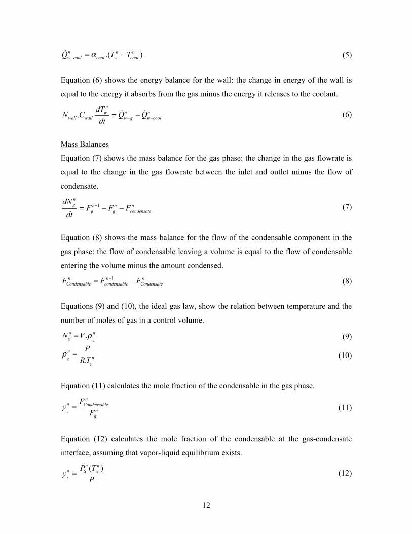
.( )n n nw cool cool w coolQ T Tα− = − (5)

Equation (6) shows the energy balance for the wall: the change in energy of the wall is

equal to the energy it absorbs from the gas minus the energy it releases to the coolant.

.n

n nwwall wall w g w cool

dTN C Q Q

dt − −= − (6)

Mass Balances

Equation (7) shows the mass balance for the gas phase: the change in the gas flowrate is

equal to the change in the gas flowrate between the inlet and outlet minus the flow of

condensate.

1ng n n n

g g condensate

dNF F F

dt−= − − (7)

Equation (8) shows the mass balance for the flow of the condensable component in the

gas phase: the flow of condensable leaving a volume is equal to the flow of condensable

entering the volume minus the amount condensed. 1n n n

Condensable condensable CondensateF F F−= − (8)

Equations (9) and (10), the ideal gas law, show the relation between temperature and the

number of moles of gas in a control volume.

.g

n ngN V ρ= (9)

.g

nn

g

PR T

ρ = (10)

Equation (11) calculates the mole fraction of the condensable in the gas phase.

g

nn Condensable

ng

FyF

= (11)

Equation (12) calculates the mole fraction of the condensable at the gas-condensate

interface, assuming that vapor-liquid equilibrium exists.

( )I

n nn S wP T

yP

= (12)

13

Diffusion Equations

The diffusion controlled model is based on the assumption that if the concentration

gradient of the condensable between the bulk gas and the gas-condensate interface favors

diffusion of the condensable species toward the interface, condensation will occur if the

vapor is saturated at the interface temperature.

Equation (13) considers the case where the concentration of condensable at the interface

is greater than the concentration in the bulk gas, thus diffusion to the interface and the

subsequent condensation will not occur.

if 0I g

n n ncondensatey y F≥ ⇒ = (13)

Equation (14) imposes the limitations of thermodynamics. In the condenser, the

temperature of the gas cannot decrease below the temperature of the wall and the coolant.

Thus, if the decrease in temperature of the gas as a result of condensation is sufficient to

bring the gas temperature to the wall temperature, no further cooling of the gas can occur.

At this point, the energy transferred between the gas and the coolant must only be the

result of condensation, not cooling, of the gas. The amount of condensate that forms is

dependent on the amount of heat that can be transferred to the coolant.

else if ( );( )

nw gn n n n n

g w g w condensate v ng w

QT T T T F

H T−≤ ⇒ = =

∆ (14)

Equation (15) describes the situation where both the concentration and temperature

gradients allow for diffusion of the condensable species to the gas-condensate interface

and condensation of the species at the interface. The flowrate of condensate is a function

of the diffusion coefficient, concentration difference, contact area, and boundary layer

thickness. The derivation of Equation (15) from Fick’s Law is shown in Appendix III.

else 1. . .ln1

I

nn AB

condensate ng

yA D CFyδ

−= −

(15)

14

Condenser Model

A program has been developed in MATLAB to simulate the operation of a

condenser. The user specifies the physical geometry of the condenser as well as the initial

temperatures and flowrates. Properties of the species, such as molecular weight,

molecular volume, density, viscosity, and Antoine equation coefficients, must also be

specified. The program uses this data to calculate the relevant heat capacities, heat

transfer coefficients, and diffusion coefficients for the system. MATLAB solvers are used

to obtain a solution to the heat and mass transfer equations, thus simulating the operation

of the condenser.

System Variable Calculations

While values for certain system properties can be found in literature, variables

such as heat capacities of mixtures, heat transfer coefficients, and diffusion coefficients

must be estimated for the given system. Many correlations regarding the calculation of

these variables can be found in literature. The correlations used in this model are detailed

in Appendix IV.

As an initial estimate, the values were calculated at the inlet gas conditions. Since

these parameters are dependent on the gas temperature and flowrates of condensable and

noncondensable species, it was necessary to analyze the impact of updating their values

according to the position of the volume element. As the gas temperature and flowrate of

condensable species decrease along the length of the condenser, the heat capacity of the

gas mixture, heat transfer coefficient of the gas, and diffusion coefficient decrease. The

heat transfer coefficients of the condensate film and coolant remain approximately

constant. The calculation involves the addition of three equations to the coupled system.

Equations must be written for the variables found explicitly in the heat and mass transfer

equations: the heat capacity of the gas mixture, the diffusion coefficient, and alpha for the

gas phase.

15

Steady State Model

In the steady state model, the MATLAB function fsolve is used to solve the

system of equations obtained from the mass and energy balances. For the steady state

system, there is no accumulation of mass or energy within a volume element. Thus, the

dN/dt and dT/dt terms must be equal to zero. Starting with the initial conditions specified

by the user, the MATLAB function fsolve performs iterative calculations to solve the

system of equations. The solution of the system is found when the residuals are equal to

zero.

The program plots the temperature, concentration, and flow profiles along the

length of the condenser. To emphasize the heat transfer limitation imposed by Equation

(14), the heat flows associated with the cooling of the gas, condensation, and heating of

the coolant are calculated and plotted. Sample plots are shown in Figure 6. The program

performs a numerical integration to determine the total amount of condensate and uses

mass balances to calculate the error associated with the flowrate calculations for the

condensable and noncondensable species. Code for the program can be found in

Appendix V. The operating conditions for the simulations shown in the following figures

are given in Table 1.

Table 1: Operating Conditions for Condenser Simulations Inlet Gas Temperature (K) 350 Inlet Coolant Temperature (K) 230 Initial Wall Temperature (K) 250 Operating Pressure (atm) 1 Condenser Length (m) 3 Shell Inner Diameter (m) 0.9079 Tube Outer Diameter (m) 0.0200 Number of Tubes 40 Coolant Flowrate (kg/s) 15 Inlet Gas Flowrate (mol/s) 75

16

0 0.5 1 1.5 2 2.5 3200

300

400Steady State Condenser

Tem

p (K

)

0 0.5 1 1.5 2 2.5 30

0.1

0.2

VO

C C

onc.

(mol

fr.)

0 0.5 1 1.5 2 2.5 35

10

15

Fcon

b (m

ol/s

)

0 0.5 1 1.5 2 2.5 30

0.2

0.4

Length (m)

Fcon

(mol

/s)

coolantgasw all

gaswall

Figure 6a: Temperature, Concentration, and Flow Profiles for Steady State Operation

0 0.5 1 1.5 2 2.5 30

0.5

1

1.5Steady State Condenser

Qga

s (k

J/s)

0 0.5 1 1.5 2 2.5 35

10

15

Qco

nd (k

J/s)

0 0.5 1 1.5 2 2.5 35

10

15

Length (m)

Qdi

sp (k

J/s)

Figure 6b: Heat Flow Profiles for Steady State Operation

17

Dynamic Model

A model has been developed in order to understand the behavior of a condenser

under dynamic operation. The program introduces a change (such as temperature,

flowrate, or composition of a stream) into the system over a specified time range and

models the response. The solver ode15s is used to obtain a solution to the mass and

energy balances both in position and time, where the initial conditions are obtained from

the steady state solution. The program outputs the temperature, concentration, flow, and

heat flow profiles for the steady state as shown in Figures 6a and 6b. Additional plots,

shown in Figures 7a and 7b, trace the temperature change of a specified volume element

with time, as well as changes in flowrate of condensate, concentration in the bulk gas,

and concentration near the wall. In the case shown, an increase in the flowrate of the

condensable species occurs quadratically between times t = 3s and t = 5s.

0 10 20 300.12

0.13

0.14

0.15

0.16

0.17

Time (s)

Fcon

d (m

ol/s

)

0 10 20 300.14

0.15

0.16

0.17

0.18

0.19

Time

Yga

s

0 10 20 301

1.05

1.1

1.15

1.2

1.25

1.3x 10-3

Time

Yw

all

0 5 10 15 20 25 30230

240

250

260

270Temporary reponse of element a

Time (s)

Tem

p (K

)

GasCoolantWall

Figure 7a: Temperature, Flow, and Concentration Profiles for Dynamic Operation where inlet flowrate of

condensable species undergoes quadratic increase between times t=3s and t=5s.

18

0 10 20 30-10

-5

0

5x 10-8

Time (s)

Nga

sErro

r (m

ol)

0 10 20 300.14

0.15

0.16

0.17

0.18

0.19

Time (s)

Yga

s

0 10 20 301

1.05

1.1

1.15

1.2

1.25

1.3x 10-3

Time (s)

Yw

all

0 5 10 15 20 25 30230

240

250

260

270Temporary reponse of element a

Time (s)

Tem

p (K

)

GasCoolantWall

Figure 7b: Temperature, Error, and Concentration Profiles for Dynamic Operation where inlet flowrate of

condensable species undergoes quadratic increase between times t=3s and t=5s.

Uncertainty Evaluation

Several sources of uncertainty are associated with the use of a computer model to

simulate the operation of a condenser. Operating conditions such as temperatures and

flowrates can vary throughout a process or may not be known accurately due to errors in

their measurement. Parameters calculated in the model, such as heat transfer and

diffusion coefficients, also possess a degree of uncertainty associated with the specific

correlation used and its applicability to the given system. When designing a condenser,

sources of uncertainty must be considered to ensure that the operation of the condenser

will conform to the set specifications.

The effect of uncertainty on the performance of the condenser was evaluated by

selecting five uncertain variables and performing simulations at different treatment levels

of these variables. Inlet gas temperature, inlet coolant temperature, and inlet flowrate of

condensable species were selected to represent uncertainty in operating conditions.

Uncertainty in estimated variables was considered by varying the heat transfer coefficient

19

of the gas and the diffusion coefficient. Using the steady state model, three cases were

considered:

• Independent variation of one variable; Cpgas, hgas, Dab constant

• Independent variation of one variable; Cpgas, hgas, Dab change with position

• Simultaneous variation of two variables; Cpgas, hgas, Dab change with position Control System

A controller was implemented in order to improve the efficiency and reduce the

operating cost the condenser. A diagram of the control system is given in Figure 8.

Without the control system, the process would have to operate continuously at the

conditions that prevented a constraint violation in the worst case scenario. Using the

control system, a specified variable is adjusted in order to influence the system toward a

given set point. An error term is calculated as the difference between the outlet gas

temperature and the set point Tsp (desired outlet gas temperature). In this case, the error

is minimized by adjusting the coolant flowrate. The coolant flowrate can be increased as

necessary to decrease the outlet gas temperature. However, if the outlet gas temperature

is initially below the set point temperature, the coolant flowrate can be decreased,

resulting in a lower cost.

Figure 8: Control System Diagram T = temperature; m = mass flowrate; n = molar flowrate;

TT = temperature transmitter; constraint = outlet gas temperature

20

In a PI controller, the control action is determined by considering a term

proportional to the error and an integral value. As seen in Equation (16), the error term is

calculated as the difference between the outlet gas temperature and the set point

temperature.

( 1)e Tg n Tsp= + − (16)

The control action, a change in the mass flowrate of coolant, is determined by Equation

(17), where kc and TI are constants. Further study of dynamic control methods will

involve optimizing the values of kc and TI. (Note: Program code defines Ti = 1/TI.)

1*( )IT

Gc kc e edt= + ∫ (17)

The units for the above variables are as follows: e [=] K; Gc [=] kg/s; kc [=] (kg/s)*(1/K);

TI [=] s.

In Figures 9a-e, the set point temperature is 268.2K, five degrees below the

maximum allowable outlet gas temperature of 273.2K. Since the outlet gas temperature is

initially below the set point temperature, the coolant flowrate can be decreased until the

outlet gas temperature equals the set point value.

Figure 9a is used as a reference point where both kc and Ti are set at zero; thus,

no control action is carried out. Figure 9b shows that including only the proportional term

results in a constant error after the system equilibrates. As seen in Figure 9c, including

both the proportional and integral terms causes the error to approach zero. A comparison

of Figures 9c-e reveals that gradual changes to the system (i.e. small kc) result in smooth

transitions, while more dramatic changes (i.e. large kc) cause oscillations about the set

point. Accordingly, an adequate safety margin must be considered when determining the

set point in order to avoid overshooting the maximum allowed temperature.

21

Figure 9a: Control Method, Reference - kc = 0; Ti = 0; Tsp = 268.2K

Figure 9b: Control Method, Proportional Term - kc = 0.1; Ti = 0; Tsp = 268.2K

22

0 50 100 150 200230

240

250

260

270Temporary reponse of element a

Time (s)

Tem

p (K

)

0 50 100 150 200266

266.5

267

267.5

268

268.5

Time (s)

Gas

Tem

p (K

)

0 50 100 150 200-2

-1.5

-1

-0.5

0

0.5

Time (s)

Erro

r (K

)

0 50 100 150 2000

5

10

15

Time (s)

Coo

lant

Flo

wra

te (k

g/s)

GasCoolantWall

Figure 9c: Control Method, Proportional (low) and Integral Terms - kc =0.1; Ti = 1.5; Tsp = 268.2K

Figure 9d: Control Method, Proportional (mid) and Integral Terms - kc = 0.3; Ti = 1.5; Tsp = 268.2K

23

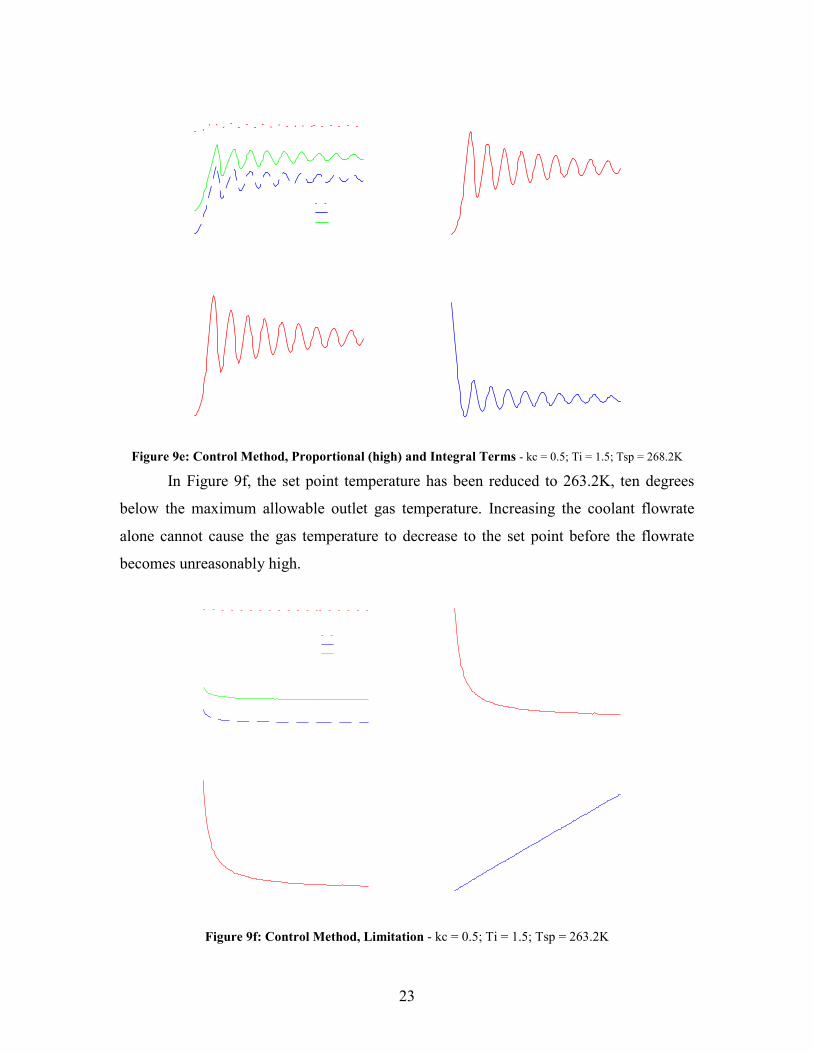
Figure 9e: Control Method, Proportional (high) and Integral Terms - kc = 0.5; Ti = 1.5; Tsp = 268.2K

In Figure 9f, the set point temperature has been reduced to 263.2K, ten degrees

below the maximum allowable outlet gas temperature. Increasing the coolant flowrate

alone cannot cause the gas temperature to decrease to the set point before the flowrate

becomes unreasonably high.

Figure 9f: Control Method, Limitation - kc = 0.5; Ti = 1.5; Tsp = 263.2K

24

The control model can also be used to simulate the system’s response to changes

in operating conditions. Figures 9g and 9h show the situation where the system is allowed

to equilibrate to the set point before a change in inlet coolant temperature is introduced.

In Figure 9g, the coolant temperature is decreased; thus, the coolant flowrate is lowered

in order to return the outlet gas temperature to the set point value. In Figure 9h, the

coolant temperature is increased; accordingly, the coolant flowrate must be increased.

Figure 9g: Control Method, Decrease in Inlet Coolant Temperature - kc = 0.1; Ti = 1.5; Tsp = 268.2K; 2% decrease

in inlet coolant temperature occurs at t = 120s

25

0 50 100 150 200 250230

240

250

260

270Temporary reponse of element a

Time (s)

Tem

p (K

)

0 50 100 150 200 250266

266.5

267

267.5

268

268.5

269

Time (s)

Gas

Tem

p (K

)0 50 100 150 200 250

-2

-1.5

-1

-0.5

0

0.5

1

Time (s)

Erro

r (K

)

0 50 100 150 200 2500

5

10

15

Time (s)C

oola

nt F

low

rate

(kg/

s)

GasCoolantWall

Figure 9h: Control Method, Increase in Inlet Coolant Temperature - kc = 0.1; Ti = 1.5; Tsp = 268.2K; 2% increase in

inlet coolant temperature occurs at t = 120s

(Remark: The dynamic control model used includes only the first approximation where

the heat capacity of the gas, heat transfer coefficient of the gas, and diffusion coefficient

are constant.)

RESULTS AND DISCUSSION

Steady State Uncertainty Evaluation

In order to determine the impact of uncertainty on condenser performance, five

uncertain variables were selected (inlet gas temperature, inlet coolant temperature, inlet

flowrate of condensable species, heat transfer coefficient of gas, and diffusion

coefficient) and trials were performed using combinations of different levels of these

variables. The treatment levels used for each variable are shown in Table A6.1. Using the

steady state model, three cases were considered:

• Independent variation of one variable; Cpgas, hgas, Dab constant

• Independent variation of one variable; Cpgas, hgas, Dab change with position

• Simultaneous variation of two variables; Cpgas, hgas, Dab change with position

26

Table 2: Treatment Levels of Uncertain Variables

Variable Nominal Action 1 2 3 4 5 6 7 8 9 10 11Tg(1) 350 add -5 -4 -3 -2 -1 0 1 2 3 4 5Tcool(1) 230 add -2 -1.6 -1.2 -0.8 -0.4 0 0.4 0.8 1.2 1.6 2Fconb(1) 15 add -1 -0.8 -0.6 -0.4 -0.2 0 0.2 0.4 0.6 0.8 1hgas calculate multiply by 0.8 0.84 0.88 0.92 0.96 1 1.04 1.08 1.12 1.16 1.2Dab calculate multiply by 0.8 0.84 0.88 0.92 0.96 1 1.04 1.08 1.12 1.16 1.2

Numerical data from the simulations is found in Appendix VI.

Independent Variation of One Variable (Cpgas, hgas, Dab change with position)

In the following simulations, the maximum allowable outlet gas temperature at

the nominal condition is 273.2K. Table 3 and Figure 10 show that the outlet gas

temperature increases with increasing inlet gas temperature. Varying the inlet gas

temperature five degrees above and below the nominal value did not result in a constraint

violation.

Table 3: Outlet Gas Temperature vs. Inlet Gas Temperature

Tg_in Delta Tg_in % Change Tg_out Delta Tg_out % Change(K) (K) (K) (K)

345 -5 -1.43 262.26 -4.39 -1.65346 -4 -1.14 263.14 -3.51 -1.32347 -3 -0.86 264.01 -2.64 -0.99348 -2 -0.57 264.89 -1.76 -0.66349 -1 -0.29 265.77 -0.88 -0.33350 0 0.00 266.65 0.00 0.00351 1 0.29 267.54 0.89 0.33352 2 0.57 268.42 1.77 0.66353 3 0.86 269.30 2.65 0.99354 4 1.14 270.19 3.54 1.33355 5 1.43 271.07 4.42 1.66

Outlet Gas Temperature vs. Inlet Gas Temperature

Outlet Gas Temperature vs. Inlet Gas Temperature y = 0.8814x - 41.819R2 = 1

261

262

263

264

265

266

267

268

269

270

271

272

344 345 346 347 348 349 350 351 352 353 354 355 356Inlet Gas Temperature (K)

Out

let G

as T

empe

ratu

re (K

)

Figure 10: Outlet Gas Temperature vs. Inlet Gas Temperature

Table 4 and Figure 11 show that the outlet gas temperature also increases with

increasing coolant temperature; however, the inlet coolant temperature has a smaller

effect on the outlet gas temperature than the inlet gas temperature. For a range of inlet

coolant temperatures two degrees above and below the nominal value, the condenser

performed within the given constraints.

27

Table 4: Outlet Gas Temperature vs. Inlet Coolant Temperature

Tcool_in Delta Tcool_in % Change Tg_out Delta Tg_out % Change(K) (K) (K) (K)228.0 -2.0 -0.87 266.38 -0.27 -0.10228.4 -1.6 -0.70 266.43 -0.22 -0.08228.8 -1.2 -0.52 266.49 -0.16 -0.06229.2 -0.8 -0.35 266.54 -0.11 -0.04229.6 -0.4 -0.17 266.60 -0.05 -0.02230.0 0.0 0.00 266.65 0.00 0.00230.4 0.4 0.17 266.71 0.06 0.02230.8 0.8 0.35 266.77 0.12 0.05231.2 1.2 0.52 266.83 0.18 0.07231.6 1.6 0.70 266.88 0.23 0.09232.0 2.0 0.87 266.94 0.29 0.11

Outlet Gas Temperature vs. Inlet Coolant Temperature

Outlet Gas Temperature vs. Inlet Coolant Temperature y = 0.1407x + 234.3R2 = 0.9996

266.3

266.4

266.5

266.6

266.7

266.8

266.9

267.0

227.6 228.0 228.4 228.8 229.2 229.6 230.0 230.4 230.8 231.2 231.6 232.0 232.4Inlet Coolant Temperature (K)

Out

let G

as T

empe

ratu

re (K

)

Figure 11: Outlet Gas Temperature vs. Inlet Coolant Temperature

Table 5 and Figure 12 show that the outlet gas temperature increases with

decreasing inlet condensable flowrate. For a range of inlet condensable flowrates one

mol/s above and below the nominal value, the condenser performed within the operating

constraints.

Table 5: Outlet Gas Temperature vs. Inlet Condensable Flowrate

Fconb_in Delta Fconb_in % Change Tg_out Delta Tg_out % Change(mol/s) (mol/s) (K) (K)

14.0 -1.0 -6.67 271.38 4.73 1.7714.2 -0.8 -5.33 270.44 3.79 1.4214.4 -0.6 -4.00 269.50 2.85 1.0714.6 -0.4 -2.67 268.55 1.90 0.7114.8 -0.2 -1.33 267.60 0.95 0.3615.0 0.0 0.00 266.65 0.00 0.0015.2 0.2 1.33 265.70 -0.95 -0.3615.4 0.4 2.67 264.75 -1.90 -0.7115.6 0.6 4.00 263.79 -2.86 -1.0715.8 0.8 5.33 262.84 -3.81 -1.4316.0 1.0 6.67 261.87 -4.78 -1.79

Outlet Gas Temperature vs. Inlet Condensable Flowrate

Outlet Gas Temperature vs. Inlet Condensable Flowrate y = -4.7536x + 337.95R2 = 1

260

262

264

266

268

270

272

13.8 14.0 14.2 14.4 14.6 14.8 15.0 15.2 15.4 15.6 15.8 16.0 16.2Inlet Condensable Flowrate (mol/s)

Out

let G

as T

empe

ratu

re (K

)

Figure 12: Outlet Gas Temperature vs. Inlet Condensable Flowrate

Table 6 and Figure 13 show that the outlet gas temperature increases with a

decrease in the heat transfer coefficient of the gas. For low values of the heat transfer

coefficient (i.e. the correlation used actually overestimates the coefficient), the

temperature constraint is violated.

28

Table 6: Outlet Gas Temperature vs. Heat Transfer Coefficient of Gas

Hgas Delta Hgas % Change Tg_out Delta Tg_out % Change(kJ/(s*m^2*K)) (kJ/(s*m^2*K)) (K) (K)

0.1061 -0.0265 -19.98 279.26 12.61 4.730.1114 -0.0212 -15.99 276.63 9.98 3.740.1167 -0.0159 -11.99 274.06 7.41 2.780.1220 -0.0106 -7.99 271.54 4.89 1.830.1273 -0.0053 -4.00 269.07 2.42 0.910.1326 0.0000 0.00 266.65 0.00 0.000.1379 0.0053 4.00 264.29 -2.36 -0.890.1432 0.0106 7.99 261.97 -4.68 -1.760.1486 0.0160 12.07 259.70 -6.95 -2.610.1539 0.0213 16.06 257.48 -9.17 -3.440.1592 0.0266 20.06 255.29 -11.36 -4.26

Outlet Gas Temperature vs. Heat Transfer Coefficient of Gas

Outlet Gas Temperature vs. Heat Transfer Coefficient of Gas (Initial Value) y = -450.94x + 326.71R2 = 0.9991

250

255

260

265

270

275

280

285

0.10 0.11 0.12 0.13 0.14 0.15 0.16 0.17Heat Transfer Coefficient of Gas (Initial Value) ( kJ / (s*m^2*K) )

Out

let G

as T

empe

ratu

re (K

)

Figure 13: Outlet Gas Temperature vs. Heat Transfer Coefficient of Gas

Table 7 and Figure 14 show that the outlet gas temperature increases with a

decrease in the diffusion coefficient. For low values of the diffusion coefficient (i.e. the

correlation used actually overestimates the diffusion coefficient), the temperature

constraint is violated.

Table 7: Outlet Gas Temperature vs. Diffusion Coefficient

Dab Delta Dab % Change Tg_out Delta Tg_out % Change(mol/(s*m^2*atm)) (mol/(s*m^2*atm)) (K) (K)

3.1948 -0.7987 -20.00 278.66 12.01 4.503.3545 -0.6390 -16.00 276.18 9.53 3.573.5143 -0.4792 -12.00 273.74 7.09 2.663.6740 -0.3195 -8.00 271.34 4.69 1.763.8338 -0.1597 -4.00 268.98 2.33 0.873.9935 0.0000 0.00 266.65 0.00 0.004.1532 0.1597 4.00 264.37 -2.28 -0.864.3130 0.3195 8.00 262.13 -4.52 -1.704.4727 0.4792 12.00 259.93 -6.72 -2.524.6325 0.6390 16.00 257.76 -8.89 -3.334.7922 0.7987 20.00 255.63 -11.02 -4.13

Outlet Gas Temperature vs. Diffusion Coefficient

Outlet Gas Temperature vs. Diffusion Coefficient (Initial Value) y = -14.415x + 324.42R2 = 0.9994

250

255

260

265

270

275

280

3.0 3.2 3.4 3.6 3.8 4.0 4.2 4.4 4.6 4.8 5.0Diffusion Coefficient (Initial Value) ( mol / (s*m^2*atm) )

Out

let G

as T

empe

ratu

re (K

)

Figure 14: Outlet Gas Temperature vs. Diffusion Coefficient

Figures 15 through 18 show the relationship between parameters. As seen in

Figure15, the diffusion coefficient is strongly dependent on the heat transfer coefficient

of the gas. Weaker relationships exist between the diffusion coefficient and inlet gas

temperature, heat transfer coefficient of the gas and inlet condensable flowrate, and

diffusion coefficient and inlet condensable flowrate.

29

Diffusion Coefficient vs. Heat Transfer Coefficient of Gas y = 30.078x + 0.0043R2 = 1

3.0

3.2

3.4

3.6

3.8

4.0

4.2

4.4

4.6

4.8

5.0

0.10 0.11 0.12 0.13 0.14 0.15 0.16 0.17Heat Transfer Coefficient of Gas (kJ / (s*m^2*K))

Diff

usio

n C

oeffi

cien

t (m

ol /

(s*m

^2*a

tm))

Figure 15: Diffusion Coefficient vs. Heat Transfer Coefficient of Gas

Diffusion Coefficient vs. Inlet Gas Temperature y = 0.0038x + 2.6622R2 = 1

3.970

3.975

3.980

3.985

3.990

3.995

4.000

4.005

4.010

4.015

344 345 346 347 348 349 350 351 352 353 354 355 356Inlet Gas Temperature (K)

Diff

usio

n C

oeffi

cien

t (m

ol /

(s*m

^2*a

tm))

Figure 16: Diffusion Coefficient vs. Inlet Gas Temperature

Heat Transfer Coefficient of Gas vs. Inlet Condensable Flowrate y = 0.0009x + 0.119R2 = 0.9975

0.1315

0.1320

0.1325

0.1330

0.1335

0.1340

13.8 14.0 14.2 14.4 14.6 14.8 15.0 15.2 15.4 15.6 15.8 16.0 16.2Inlet Condensable Flowrate (mol/s)

Hea

t Tra

nsfe

r Coe

ffici

ent o

f Gas

(kJ

/ (s*

m^2

*K))

Figure 17: Heat Transfer Coefficient of Gas vs. Inlet Condensable Flowrate

Diffusion Coefficient vs. Inlet Condensable Flowrate y = 0.0386x + 3.4139R2 = 1

3.95

3.96

3.97

3.98

3.99

4.00

4.01

4.02

4.03

4.04

13.8 14.0 14.2 14.4 14.6 14.8 15.0 15.2 15.4 15.6 15.8 16.0 16.2Inlet Condensable Flowrate (mol/s)

Diff

usio

n C

oeffi

cien

t (m

ol /

(s*m

^2*a

tm))

Figure 18: Diffusion Coefficient vs. Inlet Condensable Flowrate

The same relationships between the uncertain parameters and outlet gas

temperature as seen when the heat capacity of the gas mixture, heat transfer coefficient of

the gas, and diffusion coefficient are assumed to be constant throughout the condenser as

when they are updated with position. However, the numerical results are slightly

different. When the variables are recalculated, the outlet gas temperature increases

slightly, and the percent change from the nominal case is slightly less for the same

change in the uncertain parameter.

Simultaneous Variation of Two Variables (Cpgas, hgas, Dab change with position)

After studying the effect of uncertainty in one parameter, the effect of varying two

parameters simultaneously was examined. Since the aim of the uncertainty evaluation

was to determine when a constraint violation would occur, each parameter was varied

from the nominal value in the direction that would result in an increase in the outlet gas

temperature. For the different treatment combinations, level zero is the situation where

30

both parameters are at the nominal value. Level five is the worst case scenario where both

parameters are at their maximum deviation from the nominal value.

Table 8 and Figure 19 show that increasing the inlet gas and coolant temperatures

simultaneously does not result in a constraint violation.

Table 8: Outlet Gas Temperature vs. Inlet Gas Temperature and Inlet Coolant Temperature

Level Tg_in Delta Tg_in % Change Tcool_in Delta Tcool_in % Change Tg_out Delta Tg_out % Change(K) (K) (K) (K) (K) (K)

0 350 0 0.00 230.0 0.0 0.00 266.65 0.00 0.001 351 1 0.29 230.4 0.4 0.17 267.59 0.94 0.352 352 2 0.57 230.8 0.8 0.35 268.53 1.88 0.713 353 3 0.86 231.2 1.2 0.52 269.47 2.82 1.064 354 4 1.14 231.6 1.6 0.70 270.42 3.77 1.415 355 5 1.43 232.0 2.0 0.87 271.36 4.71 1.77

Outlet Gas Temperature vs. Inlet Gas Temperature and Inlet Coolant Temperature

Outlet Gas Temperature vs. Variation in Inlet Gas and Coolant Temperatures

y = 0.9423x + 266.65R2 = 1

266

267

268

269

270

271

272

0 1 2 3 4 5 6Level of Variation in Inlet Gas and Coolant Temperatures

Out

let G

as T

empe

ratu

re (K

)

Figure 19: Outlet Gas Temperature vs. Variation in Inlet Gas and Coolant Temperatures

31

Table 9 and Figure 20 show that increasing the inlet gas temperature and

decreasing the inlet condensable flowrate simultaneously results in a constraint violation

although performing either of these actions alone does not.

Table 9: Outlet Gas Temperature vs. Inlet Gas Temperature and Inlet Condensable Flowrate

Level Tg_in Delta Tg_in % Change Fconb_in Delta Fconb_in % Change Tg_out Delta Tg_out % Change(K) (K) (mol/s) (mol/s) (K) (K)

0 350 0 0.00 15.0 0.0 0.00 266.65 0.00 0.001 351 1 0.29 14.8 -0.2 -1.33 268.49 1.84 0.692 352 2 0.57 14.6 -0.4 -2.67 270.32 3.67 1.383 353 3 0.86 14.4 -0.6 -4.00 272.15 5.50 2.064 354 4 1.14 14.2 -0.8 -5.33 273.97 7.32 2.755 355 5 1.43 14.0 -1.0 -6.67 275.80 9.15 3.43

Outlet Gas Temperature vs. Inlet Gas Temperature and Inlet Condensable Flowrate

Outlet Gas Temperature vs. Variation in Inlet Gas Temperature

and Inlet Condensable Flowratey = 1.8291x + 266.66

R2 = 1

266

268

270

272

274

276

278

0 1 2 3 4 5 6Level of Variation in Inlet Gas Temperature and Inlet Condensable Flowrate

Out

let G

as T

empe

ratu

re (K

)

Figure 20: Outlet Gas Temperature vs. Variation in Inlet Gas Temperature and Inlet Condensable Flowrate

32

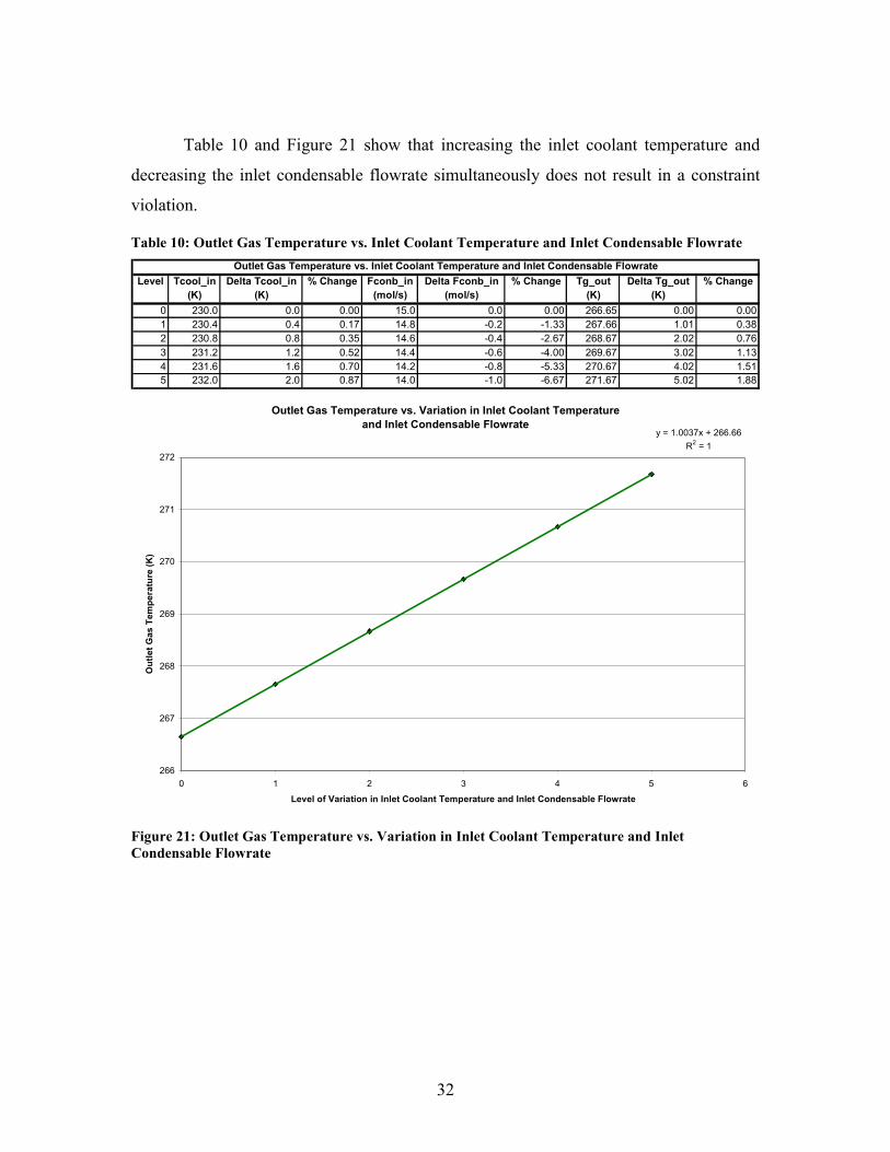
Table 10 and Figure 21 show that increasing the inlet coolant temperature and

decreasing the inlet condensable flowrate simultaneously does not result in a constraint

violation.

Table 10: Outlet Gas Temperature vs. Inlet Coolant Temperature and Inlet Condensable Flowrate

Level Tcool_in Delta Tcool_in % Change Fconb_in Delta Fconb_in % Change Tg_out Delta Tg_out % Change(K) (K) (mol/s) (mol/s) (K) (K)

0 230.0 0.0 0.00 15.0 0.0 0.00 266.65 0.00 0.001 230.4 0.4 0.17 14.8 -0.2 -1.33 267.66 1.01 0.382 230.8 0.8 0.35 14.6 -0.4 -2.67 268.67 2.02 0.763 231.2 1.2 0.52 14.4 -0.6 -4.00 269.67 3.02 1.134 231.6 1.6 0.70 14.2 -0.8 -5.33 270.67 4.02 1.515 232.0 2.0 0.87 14.0 -1.0 -6.67 271.67 5.02 1.88

Outlet Gas Temperature vs. Inlet Coolant Temperature and Inlet Condensable Flowrate

Outlet Gas Temperature vs. Variation in Inlet Coolant Temperature

and Inlet Condensable Flowratey = 1.0037x + 266.66

R2 = 1

266

267

268

269

270

271

272

0 1 2 3 4 5 6Level of Variation in Inlet Coolant Temperature and Inlet Condensable Flowrate

Out

let G

as T

empe

ratu

re (K

)

Figure 21: Outlet Gas Temperature vs. Variation in Inlet Coolant Temperature and Inlet Condensable Flowrate

33

Design Applications

A condenser model has been developed for application in processes for reducing

VOC emissions. The model can be used to aid in the design of a condenser to treat a

VOC stream, as well as control and optimization of the process.

The initial focus must be to conform to the operating constraints (maximum

allowed outlet gas temperature) determined by EPA regulations. In the initial design

stages, the steady state model can be used to determine whether a particular set of

operating conditions and condenser geometry will adhere to or violate the constraints and

adjustments can be made accordingly. The model can also be used to analyze the effect of

uncertainty in system parameters. Uncertainty is present both in the operating conditions

and the estimated parameters. The design must account for these uncertainties to ensure

that they do not result in constraint violations. Due to the complex relationships between

parameters, independent variation of one parameter at a time is not sufficient to analyze

the impact of uncertainty in that particular variable. In the previously shown case,

increasing the inlet gas temperature alone does not result in a constraint violation, nor

does decreasing the inlet flowrate of the condensable species. However, a constraint

violation does occur when these two parameters are varied simultaneously.

It must be recognized that the condenser does not always operate at steady state,

particularly during startup or when a change is introduced into the system. Thus, a

dynamic model was developed to simulate condenser operation under unsteady state

conditions. This model can be used to determine the system’s response to conditions that

change with time.

A control system has been implemented in order to prevent constraint violations.

A control variable can be adjusted in order to influence the system toward steady state

operation about a set point. As shown in Figure 9e, the control sequence can result in

oscillations about the set point; thus, an adequate safety margin must be considered when

determining the set point so that the oscillations themselves do not result in constraint

violations.

Another feature of the control system is its role in process and cost optimization.

The controller influences the system toward the set point, whether its initial state

exceeded the set point or was in an acceptable operating range. Operating expenses can

34

be minimized by moving from the ‘acceptable’ range toward the limiting condition (the

set point).

Model Robustness

The implementation of system variable calculations and outcome of case

simulations resulted in the development of an improved model which can more

accurately represent the behavior of a fluid as it passes through a condenser. When the

calculations were inserted and the simulations begun, the heat transfer limitation

described in Equation (14) had not yet been included in the model. Trials involving low

concentrations of the condensable species in the inlet gas ran as expected; however, trials

using higher concentrations yielded physically questionable results. Figures 22 and 23

show the difference in program output obtained by varying the mole fraction of the

condensable species in the inlet gas for the operating conditions described in Table 1.

0 0.5 1 1.5 2 2.5 3200

300

400Steady State Condenser

Tem

p (K

)

0 0.5 1 1.5 2 2.5 30

0.1

0.2

VO

C C

onc.

(mol

fr.)

0 0.5 1 1.5 2 2.5 35

10

15

Fcon

b (m

ol/s

)

0 0.5 1 1.5 2 2.5 30

0.2

0.4

Length (m)

Fcon

(mol

/s)

gaswall

coolantgasw all

Figure 22a: Temperature, Concentration, and Flow Profiles for 20% Inlet VOC Concentration without Heat Transfer Limitation

0 0.5 1 1.5 2 2.5 30

200

400Steady State Condenser

Tem

p (K

)

0 0.5 1 1.5 2 2.5 30

0.2

0.4

VO

C C

onc.

(mol

fr.)

0 0.5 1 1.5 2 2.5 310

20

30

Fcon

b (m

ol/s

)

0 0.5 1 1.5 2 2.5 30

0.5

1

Length (m)

Fcon

(mol

/s)

coolantgasw all

gaswall

Figure 22b: Temperature, Concentration, and Flow Profiles for 40% Inlet VOC Concentration without Heat Transfer Limitation

0 0.5 1 1.5 2 2.5 30

0.5

1

1.5Steady State Condenser

Qga

s (k

J/s)

0 0.5 1 1.5 2 2.5 35

10

15

Qco

nd (k

J/s)

0 0.5 1 1.5 2 2.5 35

10

15

Length (m)

Qdi

sp (k

J/s)

Figure 23a: Heat Flow Profiles for 20% Inlet VOC Concentration without Heat Transfer Limitation

0 0.5 1 1.5 2 2.5 3-1

0

1Steady State Condenser

Qga

s (k

J/s)

0 0.5 1 1.5 2 2.5 30

10

20

30

Qco

nd (k

J/s)

0 0.5 1 1.5 2 2.5 30

10

20

30

Length (m)

Qdi

sp (k

J/s)

Figure 23b: Heat Flow Profiles for 40% Inlet VOC Concentration without Heat Transfer Limitation

35

As seen in Figure 22b, trials using high inlet concentrations of the condensable

species resulted in the gas temperature decreasing below the temperatures of both the

wall and the coolant. However, the laws of thermodynamics restrict the temperature

changes that can actually occur in a condenser. The temperature of the gas stream cannot

fall below the wall temperature. The initial approach to this problem was to ensure that

all of the calculations in the model were dimensionally correct and that there were no

discrepancies between the derived equations and those entered into the program. After

making these corrections and obtaining similar results, the model itself was scrutinized.

A conclusion was drawn that, in order to obtain a solution to the given system of

equations, MATLAB was creating a physically invalid representation of the system. As

written, the equations stated that condensation would occur when the concentration

gradient favored diffusion of the condensable species toward the tube wall. Figure 23b

shows that the system reaches a point where the amount of heat available from the

coolant is less than the heat required to condense the amount of gas specified by the

diffusion model (Equation (15)). Since the model forced condensation to occur in this

situation, MATLAB was forced to compensate for the energy difference when computing

the solution. As seen through the combination of Equations (2), (3), and (6) for the steady

state system, the energy transferred from the wall to the coolant is equal to the heat

convection from the bulk gas to the gas-wall interface plus the energy released through

the condensation of the gas. Thus, the heat convection term was altered in order to obtain

a solution. For the energy balance to be consistent, the heat convection term must be

negative, forcing the temperature of the gas to be lower than the temperature of the wall.

Since there was no restriction on the temperature of the gas, it was allowed to decrease

below the coolant temperature as well.

The solution to this problem involved placing a temperature restriction on the

model. When the gas temperature is greater than the wall temperature, the original

diffusion controlled model holds. However, if the decrease in the temperature of the gas

as a result of condensation is sufficient to make the gas temperature equal the wall

temperature, no further cooling of the gas may occur. A heat transfer limitation is

imposed, stating that when the gas temperature equals the wall temperature, the energy

transfer between the gas and the coolant is a result of condensation only. This theory

36

holds since the gas is saturated at the wall temperature. The amount of condensate is then

equal to the amount of heat that can be transferred to the coolant divided by the amount

of heat required to condense the species (Equation (14)).

Figures 24 and 25 show the result of repeating the trials shown in Figures 22 and

23 with the addition of the heat transfer limitation.

0 0.5 1 1.5 2 2.5 3200

300

400Steady State Condenser

Tem

p (K

)

0 0.5 1 1.5 2 2.5 30

0.1

0.2

VOC

Conc

. (m

ol fr

.)

0 0.5 1 1.5 2 2.5 35

10

15

Fcon

b (m

ol/s

)

0 0.5 1 1.5 2 2.5 30

0.2

0.4

Length (m)

Fcon

(mol

/s)

coolantgasw all

gaswall

Figure 24a: Temperature, Concentration, and Flow Profiles for 20% Inlet VOC Concentration with Heat Transfer Limitation

0 0.5 1 1.5 2 2.5 3200

300

400Steady State Condenser

Tem

p (K

)

0 0.5 1 1.5 2 2.5 30

0.2

0.4

VO

C C

onc.

(mol

fr.)

0 0.5 1 1.5 2 2.5 320

25

30

Fcon

b (m

ol/s

)

0 0.5 1 1.5 2 2.5 30

0.5

1

Length (m)

Fcon

(mol

/s)

gaswall

coolantgaswall

Figure 24b: Temperature, Concentration, and Flow Profiles for 40% Inlet VOC Concentration with Heat Transfer Limitation

0 0.5 1 1.5 2 2.5 30

0.5

1

1.5Steady State Condenser

Qga

s (k

J/s)

0 0.5 1 1.5 2 2.5 35

10

15

Qco

nd (k

J/s)

0 0.5 1 1.5 2 2.5 35

10

15

Length (m)

Qdi

sp (k

J/s)

Figure 25a: Heat Flow Profiles for 20% Inlet VOC Concentration with Heat Transfer Limitation

0 0.5 1 1.5 2 2.5 30

0.5

1Steady State Condenser

Qga

s (k

J/s)

0 0.5 1 1.5 2 2.5 30

10

20

30

Qco

nd (k

J/s)

0 0.5 1 1.5 2 2.5 30

10

20

30

Length (m)

Qdi

sp (k

J/s)

Figure 25b: Heat Flow Profiles for 40% Inlet VOC Concentration with Heat Transfer Limitation

In practice, a condenser designed based on this model should operate solely in the

diffusion controlled region of the model. While the theory behind the heat transfer

limitation is valid, it was imposed as a means to prevent the gas temperature from falling

below the wall and coolant temperatures. The current model is based on diffusion

controlled condensation where the condensate forms on the outside of the tube wall. In

the region where the heat transfer limitation applies, the bulk gas is saturated and

condensation will occur in the bulk gas, not only at the gas-wall interface. Corrections to

account for changes in fluid dynamics resulting from condensation in the bulk gas have

not been included in this model.

37

CONCLUSIONS

A mathematical model has been developed which can predict the behavior of a

condenser under both steady state and unsteady state operation. This model is valid for

situations in which condensation is diffusion controlled and the inlet gas stream is a

mixture containing a condensable species and a noncondensable species. A dynamic

control system has been implemented in order to respond to changes and return the

system to steady state operation about a given set point.

The model may be used to analyze the effect of system parameters on condenser

performance, either to determine the impact of making a conscious change or to evaluate

the effect of uncertainty in the parameters. Coupled with cost data, this information may

be used to optimize the design of a condenser. With increasingly strict regulations on

VOC emissions being developed, companies are facing increased costs. The use of a

computerized mathematical model will allow them to strike the desired balance between

minimizing cost and improving performance when designing dynamic condensers to treat

VOC emission streams.

FUTURE WORK

• Run simulations and uncertainty trials for systems with different species and

condenser geometries.

• Introduce system variable calculations into model for treatment of inlet streams

containing more than one condensable species.

• Create database of relevant properties for common VOCs.

• Gather information regarding cryogenic cooling systems and cost data for the

construction and operation of a condenser.

• Compare simulation results with experimental data to judge accuracy and

determine magnitude of error in parameter estimations (Cpgas, hgas, Dab).

• Optimize design under uncertainty.

38

ACKNOWLEDGEMENTS

• Faculty, graduate students, and post-doctoral researchers within the Chemical

Engineering Department at the University of Illinois at Chicago, particularly

Professor Andreas Linninger and Andrés Malcolm.

• The National Science Foundation.

39

REFERENCES

1 United States Environmental Protection Agency. “Refrigerated Condensers for Control

of Organic Air Emissions.” December 2001.

2 Lines, J.R. and A.E. Smith. “Condensers control and reclaim VOCs.” Chemical Processing. June 2000. http://www.graham-mfg.com/downloads/19.pdf . [1 July 2004].

3 United Stated Environmental Protection Agency. Website. www.epa.gov. 4 EPA Office of Compliance. “Sector Notebook Project: Profile of the Pharmaceutical

Manufacturing Industry.” September 1997. 22. 5 Moretti, Edward C. “Reduce VOC and HAP Emissions.” CEP. June 2002. 30-40. 6 United States Environmental Protection Agency. Air Pollution Cost Control Manual. 6th

ed. December 1995. Section 3.1, Chapter 2: “Refrigerated Condensers.” 7 United States Environmental Protection Agency. “State Implementation Plans: Illinois –

Chicago Area VOC Rules - Pharmaceutical Manufacturing.” http://yosemite.epa.gov/r5/newsip.nsf/Table%20of%20Contents?OpenView&Start=1&Count=50&Collapse=1.5#1.5. [28 June 2004].

8 United States Environmental Protection Agency. “State Implementation Plans: Illinois - ERMS - Emission Reduction Market System.” http://yosemite.epa.gov/r5/newsip.nsf/Table%20of%20Contents?OpenView&Start=1&Count=50&Collapse=1.5#1.5. [28 June 2004].

9 Kinsley, George R. Jr. “Properly Purge and Inert Storage Vessels.” CEP. February

2001. 57-61.

10 United States Environmental Protection Agency. “Control of Volatile Organic Emissions from Manufacture of Synthesized Pharmaceutical Products.” December 1978.

11 Malcolm, Andrés. “Condenser Modeling: Diffusion-controlled simultaneous mass and heat transfer.” Work in progress.

12 Middleman, Stanley. An Introduction to Mass and Heat Transfer. New York, New York: John Wiley and Sons, Inc., 1998. 10-11.

13 Felder, Richard M. and Ronald W. Rousseau. Elementary Principles of Chemical

Processing. 3rd ed. New York, New York: John Wiley and Sons, Inc., 2000. 635-637.

40

14 Kern, Donald Q. Process Heat Transfer. New York, New York: McGraw-Hill Book Company, Inc., 1950. 103-105, 343-344.

15 Perry’s Chemical Engineers’ Handbook. Ed. R.H. Perry and D. W. Green. Electronic

Copy. The McGraw-Hill Companies, Inc., 1999. 5-20,11-11.

41

APPENDIX I: Regulations for VOC Emissions by Pharmaceutical Manufacturing

Facilities in Chicago, Illinois 7

Pharmaceutical manufacturing operations are subject to the following regulations

if their VOC emissions total more than 6.8 kg/day (15 lbs/day) or 2,268 kg/year (2.5

tons/year). The use of surface condensers to reduce VOC emissions must comply with the

specifications shown in Table A1.1. If another type of air pollution control equipment is

used, it must produce at least a 90 percent reduction in VOC emissions.

Table A1.1: Operating Specifications for Surface Condensers

VOC Vapor Pressure (kPa) at 293.4K (70°F) greater than

Maximum Allowable Outlet Gas Temperature (K)

Maximum Allowable Outlet Gas Temperature (°F)

3.45 298.2 77 7 283.2 50 10 273.2 32 20 258.2 5 40 248.2 -13

42

APPENDIX II: Calculation of VOC Emissions 10

Charging

The following procedure is used to calculate the emissions resulting from the charging of

a liquid VOC into a vessel. Several assumptions have been made:

- Ideal Gas Law applies

- Volume of displaced gas equals volume of liquid charged into vessel

- Displaced air is saturated with VOC at exit temperature

1. Calculate rate of air displacement in ft3/hr. 3(0.134ft /gal) (60min / hr)Vr Lr= ∗ ∗ (A2.1)

Where: Lr = liquid pumping rate in gallons/minute

3 3(25gal/min) (0.134ft /gal) (60min / hr) 201ft /hrVr = ∗ ∗ =

2. Determine the mole fraction xi of each VOC in liquid mixture.

(moles of i in liquid mix)/(total moles of liquid mix)ix = (A2.2)

1ix =

3. Calculate the vapor pressure of the pure VOC using Antoine’s equation.

10log /( )i iP a b c T= − + (A2.3) /( )10 ia b c T

iP − += (A2.4)

Where: Pi = vapor pressure of the VOC in mmHg Ti = air temperature in °C a,b,c = Antoine’s equation constants

(8.1122 1592.864 /(226.184 21.1)10 46.86mmHgiP − += =

4. Calculate the rate of VOC emission, Se, in lbs/hr for each VOC.

( ) /( )i i iSe P x Vr MW R T= ∗ ∗ ∗ ∗ (A2.5) Where: R = 999 (mmHg*ft3)/(lbmol*K) T = temperature in K MWi = molecular weight of VOC in lbs/lbmol

3 3(46.86mmHg 1 201ft /hr 46.07lb/lbmol) /(999(mmHg*ft ) /(lbmol*K) 293.4K) 1.48lbs/hrSe = ∗ ∗ ∗ ∗ =

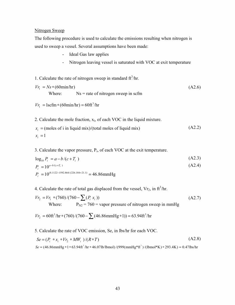
43

Nitrogen Sweep

The following procedure is used to calculate the emissions resulting when nitrogen is

used to sweep a vessel. Several assumptions have been made:

- Ideal Gas law applies

- Nitrogen leaving vessel is saturated with VOC at exit temperature

1. Calculate the rate of nitrogen sweep in standard ft3/hr.

1 (60min/hr)Vr Ns= ∗ (A2.6) Where: Ns = rate of nitrogen sweep in scfm

31 1scfm (60min/hr) 60ft /hrVr = ∗ =

2. Calculate the mole fraction, xi, of each VOC in the liquid mixture.

(moles of i in liquid mix)/(total moles of liquid mix)ix = (A2.2)

1ix =

3. Calculate the vapor pressure, Pi, of each VOC at the exit temperature.

10log /( )i iP a b c T= − + (A2.3) /( )10 ia b c T

iP − += (A2.4) (8.1122 1592.864 /(226.184 21.1)10 46.86mmHgiP − += =

4. Calculate the rate of total gas displaced from the vessel, Vr2, in ft3/hr.

2 1 (760) /(760 ( ))i iVr Vr P x= ∗ − ∑ (A2.7) Where: PN2 = 760 = vapor pressure of nitrogen sweep in mmHg

3 3

2 60ft /hr (760) /(760 (46.86mmHg 1)) 63.94ft /hrVr = ∗ − ∗ =∑

5. Calculate the rate of VOC emission, Se, in lbs/hr for each VOC.

2( ) /( )i i iSe P x Vr MW R T= ∗ ∗ ∗ ∗ (A2.8) 3 3(46.86mmHg 1 63.94ft /hr 46.07lb/lbmol) /(999(mmHg*ft ) /(lbmol*K) 293.4K) 0.47lbs/hrSe = ∗ ∗ ∗ ∗ =

44

APPENDIX III: Derivation of Diffusion Equation from Fick’s Law 12

Fick’s Law:

* * ( )A ab A A A BN C D y y N N= − ∆ + + (A3.1)

where: Ni = molar flux of species i C = total concentration Dab = diffusion coefficient yi = mole fraction of species i A = condensable species B = noncondensable species

Assume: 0BN = (A3.2)

Thus: ( * * ) /(1 )A ab A AN C D y y= − ∆ − (A3.3)

AA

dyydx

∆ = (A3.4)

( * ) /(1 )*( )AA ab A

dyN C D ydx

= − − (A3.5)

/( * ) 1/(1 )*( ) constantAA ab A

dyN C D ydx

= − − =

(A3.6)

0/( * ) 1/(1 )i

g

y

A ab A AyN C D dx y dy

δ= − −∫ ∫ (A3.7)

(1 )* /( * ) ln(1 )

IA ab

G

yN C Dy

δ −=−

(A3.8)

Where: yi = mole fraction of condensable at gas-condensate interface (x = δ) yG = mole fraction of condensable in bulk gas (x = 0)

AA

FNA

= (A3.9)

Where: FA = molar flowrate of condensable species A = area

* * (1 )*ln(1 )

ab IA

G

C D A yFyδ

−=−

(A3.10)

45

APPENDIX IV: System Variable Calculations and Correlations

Heat Capacity of Gas Mixture

Estimate Cp of each component.13

2 3Cp a b T c T d T= + ∗ + ∗ + ∗ (A5.1) or

2Cp a b T c T −= + ∗ + ∗ (A5.2) Cp [=] kJ/(mol*K); T [=] °C; a,b,c are species-dependent parameters

Calculate Cp of mixture as a weighted average.

( )i iCpgas y Cp= ∑ (A5.3)

Diffusion Coefficient14

2 /3 2/3( / ) /( ( /( )) )gf dDab h c k c p Mm kµ µ ρ= ∗ ∗ ∗ ∗ ∗ ∗ (A5.4) Dab = diffusion coefficient; lbmol/(hr*ft2atm) h = heat transfer coefficient; Btu/(hr*ft2*°F) c = specific heat of cold fluid; Btu/(lb*°F) µ = viscosity; lb/(ft*hr) k = thermal conductivity; Btu/(hr*ft*°F) pgf = log mean pressure difference of the inert gas between pg and pg’; atm pg = partial pressure of the inert gas in the gas body; atm pg’ = partial pressure of the inert gas at the condensate film; atm Mm = mean molecular weight of vapor mixture; lb/lbmol ρ = density; lb/ft3 kd = diffusivity; ft2/hr

2 /3 1/ 2 1/3 1/3 20.0166 (1/ 1/ ) /( ( ) )d A B t A Bk T M M p v v= ∗ ∗ + ∗ + (A5.5) T = temperature of gas mixture; K MA = molecular weight of diffusing species MB = molecular weight of inert species pt = total pressure; atm vA = molar volume of diffusing gas vB = molar volume of inert species

Heat Transfer Coefficients

Condensate Film15 3 2 1/ 40.73 ( / ) (( ) /( ))h k D D g k tρ λ µ= ∗ ∗ ∗ ∗ ∗ ∗ ∗ ∆ (A5.6)

1/ 4Nh h N −= ∗ (A5.7)

h = heat transfer coefficient for 1 tube; kJ/(s*m2*K) hN = heat transfer coefficient for N tubes; kJ/(s*m2*K) N = (2/3)*number of tubes across diameter of cylindrical tube bundle k = thermal heat conductivity; kJ/(s*m*K)

46

D = tube diameter; m ρ = density; kg/m3 g = gravitational constant; m/s2 λ = latent heat; kJ/kg µ = viscosity; kg/(m*s) or centipoise*10 ∆t = temperature difference between saturated vapor and surface; K

Gas14

Valid for 2,000 ≤ Re ≤ 1,000,000 0.55 1/3 0.140.36*( / )*(Re) *( * / ) *( / )wh k De c kµ µ µ= (A5.8)

Re * /De Gs µ= (A5.9) / sGs W a=

(A5.10)

( * '* ) /( *144)s Ta ID C B P= (A5.11)

square pitch: 2 24*( * / 4)

*T o

o

P dded

ππ−=

(A5.12)

triangular pitch: 24*(0.5* *0.86* 0.5* * / 4)

0.5* *T T o

o

P P dded

ππ

−= (A5.13)

h = heat transfer coefficient; Btu/(hr*ft2*°F) k = thermal conductivity; Btu/(hr*ft*°F) De = equivalent diameter, ft Re = Reynolds number c = specific heat of cold fluid; Btu/(lb*°F) µ = viscosity at bulk gas temperature; lb/(ft*hr) µw = viscosity at gas-wall interface temperature; lb/(ft*hr) Gs = mass flux of gas; lb/(hr*ft2) W = mass flowrate of gas; lb/hr as = shell-side crossflow area; ft2 ID = inner diameter of shell; inches C’ = clearance between tubes; inches B = baffle spacing; inches PT = pitch; inches de = equivalent diameter; inches do = outer diameter of tube; inches

47

APPENDIX V: Condenser Model - MATLAB Program Code

Dynamic Model

Main Program: SimCondenser_Eval_Final.m function SimCondenser(Kc,Ti,Tsp,nt,THotin,TColdin); % Uncertainty Trial Factors uf1 = 0; % Tg(1) - addition uf2 = 0; % Tcool(1) - addition uf3 = 0; % Fconb(1) - addition uf4 = 1; % hgas - multiplication uf5 = 1; % Dab - multiplication % Condenser Geometry L = 3; % total length in meters n = 30; % number of volumes to integrate length over dti = 0.019; % inner tube diameter in meters wt = 0.001; % wall thickness in meters dto = dti + wt; % outer tube diameter in meters clr = 0.02; % clearance between coolant tubes in meters pitch = clr + dto; % pitch in meters nt = 40; % number of tubes B = L; % baffle spacing in meters pt = 1; % square pitch: pt = 1, triangular pitch: pt = 2 % approximate shell diameter based on number of tubes and layout if pt == 1 number = 1; % number of tubes interior to square Area = pitch^2; % area of square in m^2 else number = 0.75; % number of tubes interior to triangle Area = 3^(1/2)/4*pitch^2; % area of triangle end element1 = nt/number; element2 = int32(element1); element3 = real(element2); elements = element3 + 1; % number of square/triangle elements for number of tubes Area_req = elements*Area; % total area of required square/triangle elements in m^2 ds = (4*3.14159*Area_req)^(1/2) % minimum required shell diameter in meters nt1 = ds/pitch; % approximate number of tubes at center of shell dz = L/n; % length increment A = 3.14159*dto*nt*dz; % contact surface area of element in m^2 Atot = 3.14159*dto*nt*L; % total contact surface area of condenser in m^2 Vt = 3.14159*dti^2/4*nt*dz; % volume inside tube per element Vw = 3.14159*dz*nt*(dto^2-dti^2)/4; % volume of wall per element Vs = 3.14159*dz*(ds^2-nt*dto^2)/4; % volume between shell and tube per element %%%%%%%%%%%%%%%%%%%%%%%%%%%%%%%%%%%%%%%%%%%%%%%%%%%%%%%%% % Operating Conditions Fcool = 15; % mass flowrate of coolant in kg/s P = 1; % total pressure in atm % Constants R = 8.314; % ideal gas constant in (m^3*Pa)/(mol*K) g = 9.81; % gravitational constant in m/s^2 %%%%%%%%%%%%%%%%%%%%%%%%%%%%%%%%%%%%%%%%%%%%%%%%%%%%%%%%%

48

% Boundary Conditions Tg(1) = 350 + uf1; % initial gas temperature in K Tcool(1) = 230 + uf2; % initial coolant temperature in K Twall(1) = 250; % initial wall temperature in K Fgas(1) = 75; % initial molar flowrate of gas in mol/s Fconb(1) = 15 + uf3; % initial molar flowrate of condensables in gas in mol/s Fcon(1) = 0; % initial molar flowrate of condensate in mol/s Ngas(1) = (Vs*P*101325)/(R*Tg(1)); % initial moles of gas Fnc = Fgas(1)-Fconb(1); % molar flowrate of noncondensables in gas in mol/s %%%%%%%%%%%%%%%%%%%%%%%%%%%%%%%%%%%%%%%%%%%%%%%%%%%%%%%%% % Initial Values for i = 1:n y0(i) = Ngas(1); y0(i+n) = Tg(1)/1.05; y0(i+2*n) = Tcool(1); y0(i+3*n) = Twall(1); y0(i+4*n) = Fgas(1); y0(i+5*n) = Fcon(1); y0(i+6*n) = Fconb(1); end %%%%%%%%%%%%%%%%%%%%%%%%%%%%%%%%%%%%%%%%%%%%%%%%%%%%%%%%% % Properties % reference: appendices of Kern: "Process Heat Transfer" Dcool = 1000; % density of coolant in kg/m^3 Dwall = 7830; % density of wall in kg/m^3 Dcond = 789; % density of condensate film in kg/m^3 Ccool = 4.184; % Cp of coolant in kJ/(kg*K) Cwall = 0.4; % Cp of wall in kJ/(kg*K) Cpc = 0.1031; % Cp of condensate in kJ/(mol*K) (Felder and Rousseau 636) Visc_gas = 0.018*2.42; % gas viscosity at temperature of bulk gas lb/(ft*hr) Visc_gas_wt = 0.015*2.42; % gas viscosity at wall temperature lb/(ft*hr) Visc_cond = 2.5*10; % viscosity of condensate film in centipoise * 10 = kg/(m*s) Visc_cool = 3.5*2.42; % coolant viscosity at temperature of bulk medium in lb/(ft*hr) Visc_cool_wt = 2.5*2.42; % coolant viscosity at wall temperature in lb/(ft*hr) M1 = 28; % molecular weight of noncondensable (nitrogen) g/mol or lb/lbmol M2 = 46.07; % molecular weight of condensable (ethanol) g/mol or lb/lbmol v1 = 2 * 15.6; % molecular volume of noncondensable (nitrogen) (Kern 344) v2 = 2 * 14.8 + 6 * 3.7 + 7.4; % molecular volume of condensable (ethanol) (Kern 344) Hv = 38.58; % heat of vaporization of condensable in kJ/mol (Felder and Rousseau 630) kg = 0.01; % thermal conductivity of gas in Btu/(hr*ft*degreesF) kf = 0.1/(9.486*10^-4)/1000/3600*3.28*1.8; % thermal conductivity of film in kJ/(s*m*K) kc = 0.3; % thermal conductivity of coolant in Btu/(hr*ft*degreesF) % Antoine Equation Coefficients for Condensable (ethanol) Aa = 8.11220; Ba = 1592.864; Ca = 226.184; % Calculations Mc = Dcool*Vt; % mass of coolant in an element in kg Nwall = Dwall*Vw; % mass of wall in a volume in kg Cvel = Fcool/Dcool/(nt*3.14159*dti^2/4); % velocity of coolant stream in m/s Tsat = Ba/(Aa-log10(Fconb(1)/Fgas(1)*P*760))-Ca+273; % saturation temperature of vapor %%%%%%%%%%%%%%%%%%%%%%%%%%%%%%%%%%%%%%%%%%%%%%%%%%%%%%%%%

49

% Unit Conversions pt = pitch*3.2808*12; % pitch in inches do = dto*3.2808*12; % outer diameter in inches di = dti*3.2808*12; % inner diameter in inches clrc = clr*3.2808*12; % clearance in inches b = B*3.2808*12; % baffle spacing in inches %%%%%%%%%%%%%%%%%%%%%%%%%%%%%%%%%%%%%%%%%%%%%%%%%%%%%%%%% % Calculate Maximum Allowable Outlet Gas Temperature % reference: EPA website: "State Implementation Plans: Illinois - Chicago Area VOC Rules - Pharmaceutical Manufacturing" Pconb = Fconb(1)/Fgas(1)*P*101.325; % inlet vapor pressure of condensable, kPa z = Tg(1)/293.4; % correction factor to operating temperature if Pconb >= 40*z Tg_max = 248.2 % maximum allowable outlet gas temperature in K elseif ((Pconb < 40*z)&(Pconb >= 20*z)) Tg_max = 258.2 elseif ((Pconb < 20*z)&(Pconb >= 10*z)) Tg_max = 273.2 elseif ((Pconb < 10*z)&(Pconb >= 7*z)) Tg_max = 283.2 elseif ((Pconb < 7*z)&(Pconb >= 3.45*z)) Tg_max = 298.2 else fprintf('Outlet gas temperature not regulated. Specify maximum value.') Tg_max = 298.2 end %%%%%%%%%%%%%%%%%%%%%%%%%%%%%%%%%%%%%%%%%%%%%%%%%%%%%%%%% % Calculate Heat Capacity of Gas Mixture % reference: Felder and Rousseau: "Elementary Principles of Chemical Processes" Table B.2 T(1) = Tg(1) - 273; % T = initial temperature of gas in degrees Celsius % component 1 = nitrogen (noncondensable) % Cp nitrogen = a + b*T + c*T^2 + d*T^3 where T is in degrees C a1 = 29 * 10^-3; b1 = 0.2199 * 10^-5; c1 = 0.5723 * 10^-8; d1 = -2.871 * 10^-12; if T(1)>0 % correlation valid for T > 0 degrees C Cp1(1) = a1 + b1*T(1) + c1*T(1)^2 + d1*T(1)^3; % Cp of noncondensable in kJ/(mol*K) else Cp1(1) = a1; end Cp_1(1) = Cp1(1)*1000*9.486*10^-4/1.8/M1*1000/2.2; % Cp of noncondensable in Btu/(lb*degF) % component 2 = ethanol (condensable) % Cp ethanol = a + b*T + c*T^2 + d*T^3 where T is in degrees C a2 = 61.34 * 10^-3; b2 = 15.72 * 10^-5; c2 = -8.749 * 10^-8; d2 = 19.83 * 10^-12; if T(1)>0 Cp2(1) = a2 + b2*T(1) + c2*T(1)^2 + d2*T(1)^3; % Cp of condensable in kJ/(mol*K) else Cp2(1) = a2;

50

end Cp_2(1) = Cp2(1)*1000*9.486*10^-4/1.8/M2*1000/2.2; % Cp of condensable in Btu/(lb*degF) % calculate Cpgas as a weighted average of the component Cps Cpgas(1) = (Fnc/Fgas(1)) * Cp1(1) + (Fconb(1)/Fgas(1)) * Cp2(1); % kJ/(mol*K) Cp_gas(1) = (Fnc*M1*Cp_1(1)+Fconb(1)*M2*Cp_2(1))/(Fnc*M1+Fconb(1)*M2); % Btu/(lb*degF) %%%%%%%%%%%%%%%%%%%%%%%%%%%%%%%%%%%%%%%%%%%%%%%%%%%%%%%%% % Calculate Heat Transfer Coefficient for Gas % reference: Kern: "Process Heat Transfer" p. 136-139 if pt == 1 de = 4*(pt^2-3.14159*do^2/4)/3.14159/do; % equivalent diameter in inches else de = 4*(0.5*pt*0.86*pt-0.5*3.14159*do^2/4)/(0.5*3.14159/do); end De = de/12; % equivalent diameter in feet Ag = di*clrc*b/pt/144; % flow area of gas in ft^2 Wg(1) = (Fnc*M1+Fconb(1)*M2)/1000*2.2*3600; % mass flow rate of gas in lb/hr Ga(1) = Wg(1)/Ag; % mass flux of gas in lb/(hr*ft^2) Reg(1) = De*Ga(1)/Visc_gas; % Reynolds number for gas % hg = heat transfer coefficient for gas in Btu/(hr*ft^2*degreesF) for 2000 < Reg < 1,000,000 hg(1) = uf4*0.36 * Reg(1)^0.55 * (Cp_gas(1)*Visc_gas/kg)^(1/3)*(Visc_gas/Visc_gas_wt)^0.14*kg/De; hgas(1) = hg(1)/(9.486*10^-4)/1000/3600*(3.28^2)*1.8; % heat transfer coefficient for gas in kJ/(s*m^2*K) %%%%%%%%%%%%%%%%%%%%%%%%%%%%%%%%%%%%%%%%%%%%%%%%%%%%%%%%% % Calculate Heat Transfer Coefficient for Condensate Film % reference: Perry's Chemical Engineer's Handbook p. 5-20, 11-11 deltaT = Tsat-Twall(1); % temp difference between sat'd vapor and surface in K % h1film = heat transfer coefficient for film with 1 tube in kJ/(s*m^2*K) h1film = 0.73*kf/dto*((dto^3*Dcond^2*g*Hv)/(kf*Visc_cond*deltaT*M2/1000))^(1/4); nt2 = 2/3*nt1; % 2/3 of max number of tubes across diameter nt3 = int32(nt2); % truncate to integer value N = real(nt3); % convert to real number hfilm = h1film*N^(-1/4); % correction for multiple tubes, kJ/(s*m^2*K) %%%%%%%%%%%%%%%%%%%%%%%%%%%%%%%%%%%%%%%%%%%%%%%%%%%%%%%%% % Calculate Heat Transfer Coefficient for Coolant % reference: Kern: "Prosess Heat Transfer" p. 103-105 Ac = 3.14159*dti^2/4*3.2808^2; % flow area of coolant in ft^2 Wc = Fcool/nt*3600*2.2; % mass flow rate of coolant per tube in lb/hr Gc = Wc/Ac; % mass flux of coolant per tube in lb/(hr*ft^2) Rec = dti*Gc/Visc_cool; % Reynolds number for coolant c = Ccool*1000*(9.486*10^-4)/2.2/1.8; % specific heat of cold fluid in Btu/(lb*degreesF) % hc = heat transfer coefficient for coolant in Btu/(hr*ft^2*degreesF) % note: eqs. valid for organic liquids, aqueous solutions, and gases, but not for water if Rec > 2100 hc = 0.027 * Rec^0.8 * (c*Visc_cool/kc)^(1/3)*(Visc_cool/Visc_cool_wt)^0.14*kc/dti; else hc = 1.86*(Rec*c*Visc_cool*dti/kc/L)^(1/3)*(Visc_cool/Visc_cool_wt)^0.14*kc/dti; end hcoolant = hc/(9.486*10^-4)/1000/3600*(3.28^2)*1.8; % heat transfer coefficient for coolant in kJ/(s*m^2*K) % correct to outer diameter of tube rather than inner diameter hcool = hcoolant*dti/dto; % heat transfer coefficient for coolant in kJ/(s*m^2/K)

51

%%%%%%%%%%%%%%%%%%%%%%%%%%%%%%%%%%%%%%%%%%%%%%%%%%%%%%%%% % Calculate General Heat Transfer Coefficients alcool = hcool*A; % alpha for cooling fluid alg(1) = 1/(1/hgas(1)+1/hfilm)*A; % alpha for gas and film U(1) = 1/(1/hgas(1) + 1/hfilm + 1/hcool); % overall heat transfer coefficient kJ/(s*m^2*K) %%%%%%%%%%%%%%%%%%%%%%%%%%%%%%%%%%%%%%%%%%%%%%%%%%%%%%%%% % Calculate Diffusion Coefficient % reference: Kern: "Process Heat Transfer" p. 343-344 % calculate diffusivity using Gilliland correlation kd(1) = 0.0166 * (Tg(1))^(3/2)/ P / (v1^(1/3) + v2^(1/3))^2 * (1/M1 + 1/M2)^(1/2); % ft^2/hr KD(1) = kd(1)/3600/3.28^2; % diffusivity in m^2/s % calculate diffusion coefficient pg1(1) = (Fnc/Fgas(1))*P; % partial pressure of the inert gas in the gas body, atm pg2(1) = P-(10^(Aa-Ba/(Twall(1)-273+Ca)))/760; % partial pressure of the inert gas at the condensate film, atm pgf(1) = (pg2(1)-pg1(1))/log(pg2(1)/pg1(1)); % log mean pressure difference of the inert gas between pg1 and pg2, atm Mm(1) = ((Fnc/Fgas(1))*M1 + (Fconb(1)/Fgas(1))*M2); % mean molecular weight of the vapor mixture, lb/lbmol Dgas(1) = P*Mm(1)/0.7302/(1.8*Tg(1)); % density of gas in lb/ft^3 % Kg = diffusion coefficient in lbmol/(hr*ft^2*atm) Kg(1) = hg(1)*((Cp_gas(1)*Visc_gas/kg)^(2/3))/(Cp_gas(1)*pgf(1)*Mm(1)*(Visc_gas/Dgas(1)/kd)^(2/3)); Dab(1) = uf5*Kg(1)*(3.2808^2)/3600*453.593; % diffusion coefficient in mol/(s*m^2*atm) %%%%%%%%%%%%%%%%%%%%%%%%%%%%%%%%%%%%%%%%%%%%%%%%%%%%%%%%% % Set Initial Values of Heat Capacities, Heat Transfer Coefficients, and Diffusion Coefficient for i=1:n % Heat Capacity cpg(i) = T(1); cpg(i+n) = Cp1(1); cpg(i+2*n) = Cp_1(1); cpg(i+3*n) = Cp2(1); cpg(i+4*n) = Cp_2(1); y0(i+7*n) = Cpgas(1); cpg(i+5*n) = Cp_gas(1); % Heat Transfer Coefficient htc(i) = Wg(1); htc(i+n) = Ga(1); htc(i+2*n) = Reg(1); htc(i+3*n) = hg(1); htc(i+4*n) = hgas(1); y0(i+8*n) = alg(1); htc(i+5*n) = U(1); % Diffusion Coefficient difc(i) = kd(1); difc(i+n) = KD(1); difc(i+2*n) = pg1(1); difc(i+3*n) = pg2(1); difc(i+4*n) = pgf(1); difc(i+5*n) = Mm(1); difc(i+6*n) = Dgas(1); difc(i+7*n) = Kg(1); y0(i+9*n) = Dab(1); end %%%%%%%%%%%%%%%%%%%%%%%%%%%%%%%%%%%%%%%%%%%%%%%%%%%%%%%%%

52

% Steady State Solution options0 = optimset('Display','iter','MaxFunEvals',1e5); [yss,fval,exitflag] = fsolve(@CondenserSS_Eval4,y0,options0,Tg,Tcool,Twall,Fgas,Fcon,Fconb,Fnc,Fcool,A,alcool,Vs,P,R,Mc,Ccool,Cwall,Cpc,Nwall,Aa,Ba,Ca,Hv,n,dz,cpg,htc,difc,Visc_gas,Visc_gas_wt,De,Ag,kg,kf,g,Visc_cond,N,M1,M2,dto,Dcond,v1,v2,hcool,a1,b1,c1,d1,a2,b2,c2,d2,L,Tsat,hfilm,hgas,U,Cpgas,Dab,uf4,uf5); yss; % Plot Results PlotSS_Eval(yss,n,Aa,Ba,Ca,P,dz,Tg,Tcool,Twall,Fgas,Fcon,Fconb,Fcool,alg,alcool,Hv,Cpc); % Extract Variables from Steady State Solution for i=1:n Ngas(i+1) = real(yss(i)); Tg(i+1) = real(yss(i+n)); Tcool(i+1) = real(yss(i+2*n)); Twall(i+1) = real(yss(i+3*n)); Fgas(i+1) = real(yss(i+4*n)); Fcon(i+1) = real(yss(i+5*n)); Fconb(i+1) = real(yss(i+6*n)); ygas(i+1) = Fconb(i+1)/Fgas(i+1); Cpgas(i+1) = yss(i+7*n); alg(i+1) = yss(i+8*n); Dab(i+1) = yss(i+9*n); end % Error Calculations Input=(Fgas(1)); TotalCond=trapz(Fcon); FgasO=Fgas(n+1); FcondbO=Fconb(n+1); Accumulated=Vs*P*101325/(R*Tg(n+1)^2)*(Tg(1)-Tg(n+1)); Output=TotalCond+FgasO+Accumulated; Fconblein=Fconb(1); CAbsErr=Fconb(1)-TotalCond-FcondbO; CondbleError=(abs(CAbsErr))/(Fconb(1))*100; NonCondError=Fnc-(FgasO*(1-ygas(n+1))); % % Print results to file % fid = fopen('Uncertainty_Evaluation_Change3.txt', 'a'); % % fprintf(fid, 'Tg_in Tcool_in Fconb_in hgas Dab Tg_out Tcool_out Fconb_out Accum Error_C Error_NC uf1 uf2 uf3 uf4 uf5 exitflag \n' ); % fprintf(fid, '%.1f %.1f %.1f %.4f %.4f %.2f %.2f %.2f %.3g %.3g %.3g %.0f %.1f %.1f %.2f %.2f %.3g \n', Tg(1), Tcool(1), Fconb(1), hgas(1), Dab(1), Tg(n+1), Tcool(n+1), Fconb(n+1), Accumulated, CondbleError, NonCondError, uf1, uf2, uf3, uf4, uf5, exitflag); % fclose(fid); % % fid2 = fopen('Variables_Change3.txt', 'a'); % % fprintf(fid2, 'n dz \n Cpgas \n Dab \n alg \n \n'); % fprintf(fid2, '%.0f %.3f \n %.5f \n %.3f \n %.4g \n \n', n, dz, Cpgas, Dab, alg); % fclose(fid2); %%%%%%%%%%%%%%%%%%%%%%%%%%%%%%%%%%%%%%%%%%%%%%%%%%%%%%%%% % Dynamic Solution tend = 30; Mstep = tend/100; tspan = [0:tend]; % time horizon integrated

53

nalg = 6; % number of algebraic eq ndiff = 4; % number of differential equations M = zeros((nalg+ndiff)*n:(nalg+ndiff)*n); % mass matrix for DAE for j=1:(ndiff)*n M(j,j) = 1; end options = odeset('Mass',M,'Refine',5,'MaxStep',Mstep); [t,y] = ode15s(@CondenserDyn_Eval_update,tspan,yss,options,Tg,Tcool,Twall,Fgas,Fcon,Fconb,Fnc,Fcool,A,alcool,Vs,P,R,Mc,Ccool,Cwall,Cpc,Nwall,Aa,Ba,Ca,Hv,Ngas,n,cpg,htc,difc,Visc_gas,Visc_gas_wt,De,Ag,kg,kf,g,Visc_cond,N,M1,M2,dto,Dcond,v1,v2,hcool,a1,b1,c1,d1,a2,b2,c2,d2,L,Tsat,hfilm,uf4,uf5); % Plot Results a = n; % length to be dispalyed in time PlotDynCond3(t,y,n,Aa,Ba,Ca,P,a,R,Vs); PlotDynError(t,y,n,Aa,Ba,Ca,P,a,R,Vs); %%%%%%%%%%%%%%%%%%%%%%%%%%%%%%%%%%%%%%%%%%%%%%%%%%%%%%%%% Steady State Solution: CondenserSS_Eval4.m function [out] = CondenserSS_Eval(y,Tg,Tcool,Twall,Fgas,Fcon,Fconb,Fnc,Fcool,A,alcool,Vs,P,R,Mc,Ccool,Cwall,Cpc,Nwall,Aa,Ba,Ca,Hv,n,dz,cpg,htc,difc,Visc_gas,Visc_gas_wt,De,Ag,kg,kf,g,Visc_cond,N,M1,M2,dto,Dcond,v1,v2,hcool,a1,b1,c1,d1,a2,b2,c2,d2,L,Tsat,hfilm,hgas,U,Cpgas,Dab,uf4,uf5) % Variables Declaration for i=1:n Ngas(i+1) = real(y(i)); Tg(i+1) = real(y(i+n)); Tcool(i+1) = real(y(i+2*n)); Twall(i+1) = real(y(i+3*n)); Fgas(i+1) = real(y(i+4*n)); Fcon(i+1) = real(y(i+5*n)); Fconb(i+1) = real(y(i+6*n)); Cpgas(i+1) = real(y(i+7*n)); alg(i+1) = real(y(i+8*n)); Dab(i+1) = real(y(i+9*n)); end for i=1:n % Heat Capacity Values T(i+1) = cpg(i); Cp1(i+1) = cpg(i+n); Cp_1(i+1) = cpg(i+2*n); Cp2_(i+1) = cpg(i+3*n); Cp_2(i+1) = cpg(i+4*n); Cp_gas(i+1) = cpg(i+5*n); % Heat Transfer Coefficient Values Wg(i+1) = htc(i); Ga(i+1) = htc(i+n); Reg(i+1) = htc(i+2*n); hg(i+1) = htc(i+3*n); hgas(i+1) = htc(i+4*n); U(i+1) = htc(i+5*n); % Diffusion Coefficient Values kd(i+1) = difc(i); KD(i+1) = difc(i+n);

54

pg1(i+1) = difc(i+2*n); pg2(i+1) = difc(i+3*n); pgf(i+1) = difc(i+4*n); Mm(i+1) = difc(i+5*n); Dgas(i+1) = difc(i+6*n); Kg(i+1) = difc(i+7*n); end %%%%%%%%%%%%%%%%%%%%%%%%%%%%%%%%%%%%%%%%%%%%%%%%%%%%%%%%% % System of Equations Declaration % Differential Equations for i=1:n % Mass Balance For Gas out(i)=Fgas(i)-Fgas(i+1)-Fcon(i+1); % Gas energy Balance out(i+n)=(Fgas(i)*Cpgas(i+1)*(Tg(i)-Tg(i+1))-alg(i+1)*(Tg(i+1)-Twall(i+1))-Fcon(i+1)*Hv)/(Ngas(i+1)*Cpgas(i+1)); % Coolant energy Balance out(i+2*n)=(Fcool*Ccool*(Tcool(i)-Tcool(i+1))+alcool*(Twall(i+1)-Tcool(i+1)))/(Mc*Ccool); % Wall energy Balance out(i+3*n)=(alg(i+1)*(Tg(i+1)-Twall(i+1))+Fcon(i+1)*(Hv+Cpc*(Tg(i+1)-Twall(i+1)))-alcool*(Twall(i+1)-Tcool(i+1)))/(Nwall*Cwall); end % Algebraic Equations for i=1:n ywall(i+1)=10^(Aa - Ba/(Twall(i+1)-273+Ca))/760/P; ygas(i+1)=Fconb(i+1)/Fgas(i+1); % Diffusion Equation if (ygas(1+i)-ywall(i+1)) <= 1e-6 out(i+4*n)=Fcon(i+1)-0; elseif (Tg(i+1)-Twall(i+1)) <= 1e-3 if Tg(i+1)-Twall(i+1) < 0 Tg(i+1) = Twall(i+1); end out(i+4*n)=Fcon(i+1)-alcool*(Twall(i+1)-Tcool(i+1))/Hv; else out(i+4*n)=Fcon(i+1)-A*Dab(i+1)*P*log((1-ywall(1+i))/(1-ygas(i+1))); end % Mass Balance For Condensable in Gas phase out(i+5*n)=Fconb(i)-Fconb(i+1)-Fcon(i+1); % Finite Volume Moles Change Due to Temperature using IG EoS out(i+6*n)=Ngas(i+1)-Vs*P/(R*Tg(i+1)); end %%%%%%%%%%%%%%%%%%%%%%%%%%%%%%%%%%%%%%%%%%%%%%%%%%%%%%%%% % Update Heat Capacity, Heat Transfer Coefficients, and Diffusion Coefficient for i=1:n % Heat Capacity T(i+1) = Tg(i+1) - 273; % T = initial temperature of gas in degrees Celsius % component 1 = nitrogen (noncondensable) if T(i+1)>0

55

Cp1(i+1) = a1 + b1*T(i+1) + c1*T(i+1)^2 + d1*T(i+1)^3; % Cp of noncondensable in kJ/(mol*K) else Cp1(i+1) = a1; end Cp_1(i+1) = Cp1(i+1)*1000*9.486*10^-4/1.8/M1*1000/2.2; % Cp of noncondensable in Btu/(lb*degF) % component 2 = ethanol (condensable) if T(i+1)>0 Cp2(i+1) = a2 + b2*T(i+1) + c2*T(i+1)^2 + d2*T(i+1)^3; % Cp of condensable in kJ/(mol*K) else Cp2(i+1) = a2; end Cp_2(i+1) = Cp2(i+1)*1000*9.486*10^-4/1.8/M2*1000/2.2; % Cp of condensable in Btu/(lb*degF) % calculate Cpgas as a weighted average of the component Cps out(i+7*n) = (Fnc/Fgas(i+1)) * Cp1(i+1) + (Fconb(i+1)/Fgas(i+1)) * Cp2(i+1) - Cpgas(i+1); % kJ/(mol*K) Cp_gas(i+1) = (Fnc*M1*Cp_1(i+1)+Fconb(i+1)*M2*Cp_2(i+1))/(Fnc*M1+Fconb(i+1)*M2); % Btu/(lb*degF) % Heat Transfer Coefficient of Gas Wg(i+1) = (Fnc*M1+Fconb(i+1)*M2)/1000*2.2*3600; % mass flow rate of gas in lb/hr Ga(i+1) = Wg(i+1)/Ag; % mass flux of gas in lb/(hr*ft^2) Reg(i+1) = De*Ga(i+1)/Visc_gas; % Reynolds number for gas hg(i+1) = uf4*0.36 * Reg(i+1)^0.55 * (Cp_gas(i+1)*Visc_gas/kg)^(1/3)*(Visc_gas/Visc_gas_wt)^0.14*kg/De; % Btu/(hr*ft^2*degreesF) hgas(i+1) = hg(i+1)/(9.486*10^-4)/1000/3600*(3.28^2)*1.8; % heat transfer coefficient for gas in kJ/(s*m^2*K) % General Heat Transfer Coefficients out(i+8*n) = 1/(1/hgas(i+1)+1/hfilm)*A - alg(i+1); % alpha for gas and film U(i+1) = 1/(1/hgas(i+1) + 1/hfilm + 1/hcool); % overall heat transfer coefficient kJ/(s*m^2*K) % Diffusion Coefficient kd(i+1) = 0.0166 * (Tg(i+1))^(3/2)/ P / (v1^(1/3) + v2^(1/3))^2 * (1/M1 + 1/M2)^(1/2); % diffusivity in ft^2/hr KD(i+1) = kd(i+1)/3600/3.28^2; % diffusivity in m^2/s pg1(i+1) = (Fnc/Fgas(i+1))*P; % partial pressure of the inert gas in the gas body, atm pg2(i+1) = P-(10^(Aa-Ba/(Twall(i+1)-273+Ca)))/760; % partial pressure of the inert gas at the condensate film, atm pgf(i+1) = (pg2(i+1)-pg1(i+1))/log(pg2(i+1)/pg1(i+1)); % log mean pressure difference of the inert gas between pg1 and pg2, atm Mm(i+1) = ((Fnc/Fgas(i+1))*M1 + (Fconb(i+1)/Fgas(i+1))*M2); % mean molecular weight of the vapor mixture, lb/lbmol Dgas(i+1) = P*Mm(i+1)/0.7302/(1.8*Tg(i+1)); % density of gas in lb/ft^3 % Kg = diffusion coefficient in lbmol/(hr*ft^2*atm) Kg(i+1) = hg(i+1)*((Cp_gas(i+1)*Visc_gas/kg)^(2/3))/(Cp_gas(i+1)*pgf(i+1)*Mm(i+1)*(Visc_gas/Dgas(i+1)/kd(i+1))^(2/3)); out(i+9*n) = uf5*Kg(i+1)*(3.2808^2)/3600*453.593 - Dab(i+1); % diffusion coefficient in mol/(s*m^2*atm) end %%%%%%%%%%%%%%%%%%%%%%%%%%%%%%%%%%%%%%%%%%%%%%%%%%%%%%%%% out=out'; %%%%%%%%%%%%%%%%%%%%%%%%%%%%%%%%%%%%%%%%%%%%%%%%%%%%%%%%% Steady State Plot: PlotSS_Eval.m function []=PlotSS_Eval(yss,n,Aa,Ba,Ca,P,dz,Tg,Tcool,Twall,Fgas,Fcon,Fconb,Fcool,alg,alcool,Hv,Cpc); %Variables Declaration for i=1:n Tg(i)=real(yss(i+n)); Tcool(i)=real(yss(i+2*n)); Twall(i)=real(yss(i+3*n)); Fgas(i)=real(yss(i+4*n));

56

Fcon(i)=real(yss(i+5*n)); Fconb(i)=real(yss(i+6*n)); end for i=1:n ygas(i)=Fconb(i)/Fgas(i); ywall(i)=10^(Aa - Ba/(Twall(i)-273+Ca))/760/P; end le=1:n; lee=0+dz*le; figure(1); subplot(4,1,1),plot(lee,Tcool,'--', lee,Tg,'.:r',lee,Twall,'g') title('Steady State Condenser'); legend('coolant', 'gas', 'wall'); % xlabel('Length'); ylabel('Temp (K)') subplot(4,1,2),plot(lee,ygas,'.:r',lee,ywall,'g') % title('Fg out vs L'); legend('gas', 'wall'); % xlabel('Time'); ylabel('VOC Conc. (mol fr.)') subplot(4,1,3),plot(lee,Fconb,'g') % title('Control vs time'); % xlabel('Length'); ylabel('Fconb (mol/s)') subplot(4,1,4),plot(lee,Fcon,'b') % title('Control vs time'); xlabel('Length (m)'); ylabel('Fcon (mol/s)') figure(2); qgas=alg*(Tg-Twall); qcond=Fcon.*(Hv+Cpc*(Tg-Twall)); qdisp=alcool*(Twall-Tcool); diff=qdisp-qgas; subplot(3,1,1),plot(lee,qgas) title('Steady State Condenser'); % xlabel('Length'); ylabel('Qgas (kJ/s)') subplot(3,1,2),plot(lee,qcond,lee,diff,'r.') % title('Fg out vs L'); % xlabel('Time'); ylabel('Qcond (kJ/s)') subplot(3,1,3),plot(lee,qdisp) % title('Control vs time'); xlabel('Length (m)'); ylabel('Qdisp (kJ/s)') Dynamic Solution: CondenserDyn_Eval_update.m function [out] = CondenserDyn_Eval_update(t,y,Tg,Tcool,Twall,Fgas,Fcon,Fconb,Fnc,Fcool,A,alcool,Vs,P,R,Mc,Ccool,Cwall,Cpc,Nw

57

all,Aa,Ba,Ca,Hv,Ngas,n,cpg,htc,difc,Visc_gas,Visc_gas_wt,De,Ag,kg,kf,g,Visc_cond,N,M1,M2,dto,Dcond,v1,v2,hcool,a1,b1,c1,d1,a2,b2,c2,d2,L,Tsat,hfilm,uf4,uf5) % Variables Declaration for i=1:n Ngas(i+1) = real(y(i)); Tg(i+1) = real(y(i+n)); Tcool(i+1) = real(y(i+2*n)); Twall(i+1) = real(y(i+3*n)); Fgas(i+1) = real(y(i+4*n)); Fcon(i+1) = real(y(i+5*n)); Fconb(i+1) = real(y(i+6*n)); Cpgas(i+1) = real(y(i+7*n)); alg(i+1) = real(y(i+8*n)); Dab(i+1) = real(y(i+9*n)); end for i=1:n % Heat Capacity Values T(i+1) = cpg(i); Cp1(i+1) = cpg(i+n); Cp_1(i+1) = cpg(i+2*n); Cp2_(i+1) = cpg(i+3*n); Cp_2(i+1) = cpg(i+4*n); Cp_gas(i+1) = cpg(i+5*n); % Heat Transfer Coefficient Values Wg(i+1) = htc(i); Ga(i+1) = htc(i+n); Reg(i+1) = htc(i+2*n); hg(i+1) = htc(i+3*n); hgas(i+1) = htc(i+4*n); U(i+1) = htc(i+5*n); % Diffusion Coefficient Values kd(i+1) = difc(i); KD(i+1) = difc(i+n); pg1(i+1) = difc(i+2*n); pg2(i+1) = difc(i+3*n); pgf(i+1) = difc(i+4*n); Mm(i+1) = difc(i+5*n); Dgas(i+1) = difc(i+6*n); Kg(i+1) = difc(i+7*n); end %%%%%%%%%%%%%%%%%%%%%%%%%%%%%%%%%%%%%%%%%%%%%%%%%%%%%%%%% % Simulation Changes Fconb0=Fconb(1); if (t >= 3) & (t < 5) Fconb(1)=Fconb0+1*(t-3)^2; elseif t >= 5 Fconb(1)=Fconb0+1*(5-3)^2; end %%%%%%%%%%%%%%%%%%%%%%%%%%%%%%%%%%%%%%%%%%%%%%%%%%%%%%%%% % System of Equations Declaration % Differential Equations for i=1:n

58

% Mass Balance For Gas out(i)=-Vs*P/(R*(Tg(i+1))^2)*(Fgas(i)*Cpgas(i+1)*(Tg(i)-Tg(i+1))-alg(i+1)*(Tg(i+1)-Twall(i+1))-Fcon(i+1)*Hv)/(Ngas(i+1)*Cpgas(i+1)); % Gas energy Balance out(i+n)=(Fgas(i)*Cpgas(i+1)*(Tg(i)-Tg(i+1))-alg(i+1)*(Tg(i+1)-Twall(i+1))-Fcon(i+1)*Hv)/(Ngas(i+1)*Cpgas(i+1)); % Coolant energy Balance out(i+2*n)=(Fcool*Ccool*(Tcool(i)-Tcool(i+1))+alcool*(Twall(i+1)-Tcool(i+1)))/(Mc*Ccool); % Wall energy Balance out(i+3*n)=(alg(i+1)*(Tg(i+1)-Twall(i+1))+Fcon(i+1)*(Hv+Cpc*(Tg(i+1)-Twall(i+1)))-alcool*(Twall(i+1)-Tcool(i+1)))/(Nwall*Cwall); end % Algebraic Equations for i=1:n ywall(i+1)=10^(Aa - Ba/(Twall(i+1)-273+Ca))/760/P; ygas(i+1)=Fconb(i+1)/Fgas(i+1); % Diffusion Equation if (ygas(i+1)-ywall(i+1)) <= 1e-6 out(i+4*n)=Fcon(i+1)-0; elseif (Tg(i+1)-Twall(i+1)) <= 1e-3 if Tg(i+1)-Twall(i+1) < 0 Tg(i+1) = Twall(i+1); end out(i+4*n)=Fcon(i+1)-alcool*(Twall(i+1)-Tcool(i+1))/Hv; else out(i+4*n)=Fcon(i+1)-A*Dab(i+1)*P*log((1-ywall(1+i))/(1-ygas(i+1))); end % Mass Balance For Condensable in Gas phase out(i+5*n)=Fconb(i)-Fconb(i+1)-Fcon(i+1); % Finite Volume Moles Change Due to Temperature using IG EoS out(i+6*n)=Fgas(i)-Fgas(i+1)-Fcon(i+1)+Vs*P/(R*(Tg(i+1))^2)*(Fgas(i)*Cpgas(i+1)*(Tg(i)-Tg(i+1))-alg(i+1)*(Tg(i+1)-Twall(i+1))-Fcon(i+1)*Hv)/(Ngas(i+1)*Cpgas(i+1)); end %%%%%%%%%%%%%%%%%%%%%%%%%%%%%%%%%%%%%%%%%%%%%%%%%%%%%%%%% % Update Heat Capacity, Heat Transfer Coefficients, and Diffusion Coefficient for i=1:n % Heat Capacity T(i+1) = Tg(i+1) - 273; % T = initial temperature of gas in degrees Celsius % component 1 = nitrogen (noncondensable) if T(i+1)>0 Cp1(i+1) = a1 + b1*T(i+1) + c1*T(i+1)^2 + d1*T(i+1)^3; % Cp of noncondensable in kJ/(mol*K) else Cp1(i+1) = a1; end Cp_1(i+1) = Cp1(i+1)*1000*9.486*10^-4/1.8/M1*1000/2.2; % Cp of noncondensable in Btu/(lb*degF) % component 2 = ethanol (condensable) if T(i+1)>0 Cp2(i+1) = a2 + b2*T(i+1) + c2*T(i+1)^2 + d2*T(i+1)^3; % Cp of condensable in kJ/(mol*K) else Cp2(i+1) = a2; end Cp_2(i+1) = Cp2(i+1)*1000*9.486*10^-4/1.8/M2*1000/2.2; % Cp of condensable in Btu/(lb*degF) % calculate Cpgas as a weighted average of the component Cps

59

out(i+7*n) = (Fnc/Fgas(i+1)) * Cp1(i+1) + (Fconb(i+1)/Fgas(i+1)) * Cp2(i+1) - Cpgas(i+1); % kJ/(mol*K) Cp_gas(i+1) = (Fnc*M1*Cp_1(i+1)+Fconb(i+1)*M2*Cp_2(i+1))/(Fnc*M1+Fconb(i+1)*M2); % Btu/(lb*degF) % Heat Transfer Coefficient of Gas Wg(i+1) = (Fnc*M1+Fconb(i+1)*M2)/1000*2.2*3600; % mass flow rate of gas in lb/hr Ga(i+1) = Wg(i+1)/Ag; % mass flux of gas in lb/(hr*ft^2) Reg(i+1) = De*Ga(i+1)/Visc_gas; % Reynolds number for gas hg(i+1) = uf4*0.36 * Reg(i+1)^0.55 * (Cp_gas(i+1)*Visc_gas/kg)^(1/3)*(Visc_gas/Visc_gas_wt)^0.14*kg/De; % Btu/(hr*ft^2*degreesF) hgas(i+1) = hg(i+1)/(9.486*10^-4)/1000/3600*(3.28^2)*1.8; % heat transfer coefficient for gas in kJ/(s*m^2*K) % General Heat Transfer Coefficients out(i+8*n) = 1/(1/hgas(i+1)+1/hfilm)*A - alg(i+1); % alpha for gas and film U(i+1) = 1/(1/hgas(i+1) + 1/hfilm + 1/hcool); % overall heat transfer coefficient kJ/(s*m^2*K) % Diffusion Coefficient kd(i+1) = 0.0166 * (Tg(i+1))^(3/2)/ P / (v1^(1/3) + v2^(1/3))^2 * (1/M1 + 1/M2)^(1/2); % diffusivity in ft^2/hr KD(i+1) = kd(i+1)/3600/3.28^2; % diffusivity in m^2/s pg1(i+1) = (Fnc/Fgas(i+1))*P; % partial pressure of the inert gas in the gas body, atm pg2(i+1) = P-(10^(Aa-Ba/(Twall(i+1)-273+Ca)))/760; % partial pressure of the inert gas at the condensate film, atm pgf(i+1) = (pg2(i+1)-pg1(i+1))/log(pg2(i+1)/pg1(i+1)); % log mean pressure difference of the inert gas between pg1 and pg2, atm Mm(i+1) = ((Fnc/Fgas(i+1))*M1 + (Fconb(i+1)/Fgas(i+1))*M2); % mean molecular weight of the vapor mixture, lb/lbmol Dgas(i+1) = P*Mm(i+1)/0.7302/(1.8*Tg(i+1)); % density of gas in lb/ft^3 % Kg = diffusion coefficient in lbmol/(hr*ft^2*atm) Kg(i+1) = hg(i+1)*((Cp_gas(i+1)*Visc_gas/kg)^(2/3))/(Cp_gas(i+1)*pgf(i+1)*Mm(i+1)*(Visc_gas/Dgas(i+1)/kd(i+1))^(2/3)); out(i+9*n) = uf5*Kg(i+1)*(3.2808^2)/3600*453.593 - Dab(i+1); % diffusion coefficient in mol/(s*m^2*atm) end %%%%%%%%%%%%%%%%%%%%%%%%%%%%%%%%%%%%%%%%%%%%%%%%%%%%%%%%% out = out'; %%%%%%%%%%%%%%%%%%%%%%%%%%%%%%%%%%%%%%%%%%%%%%%%%%%%%%%%% Dynamic Plot 1: PlotDynCond3.m function []=PlotDynCond(t,y,n,Aa,Ba,Ca,P,a,R,Vs) tfin = size(y); for i=1:tfin Ngas(i)=(y(i,a)); Tg(i)=(y(i,n+a)); Tcool(i)=(y(i,2*n+a)); Twall(i)=(y(i,3*n+a)); Fgas(i)=(y(i,4*n+a)); Fcon(i)=(y(i,5*n+a)); Fconb(i)=(y(i,6*n+a)); ygas(i)=Fconb(i)/Fgas(i); ywall(i)=10^(Aa - Ba/(Twall(i)-273+Ca))/760/P; diff(i)=Ngas(i)-Vs*P/(R*Tg(i)); end figure(3); subplot(2,3,4),plot(t,Fcon) xlabel('Time (s)'); ylabel('Fcond (mol/s)');

60

subplot(2,3,5),plot(t,ygas,'r') xlabel('Time'); ylabel('Ygas'); subplot(2,3,6),plot(t,ywall,'g') xlabel('Time'); ylabel('Ywall'); subplot(2,1,1),plot(t,Tg,'.:r',t,Tcool,'--b',t,Twall,'g') title('Temporary reponse of element a'); xlabel('Time (s)'); ylabel('Temp (K)'); legend('Gas', 'Coolant', 'Wall'); Dynamic Plot 2: PlotDynError.m function []=PlotDynCond(t,y,n,Aa,Ba,Ca,P,a,R,Vs) tfin = size(y); for i=1:tfin Ngas(i)=(y(i,a)); Tg(i)=(y(i,n+a)); Tcool(i)=(y(i,2*n+a)); Twall(i)=(y(i,3*n+a)); Fgas(i)=(y(i,4*n+a)); Fcon(i)=(y(i,5*n+a)); Fconb(i)=(y(i,6*n+a)); ygas(i)=Fconb(i)/Fgas(i); ywall(i)=10^(Aa - Ba/(Twall(i)-273+Ca))/760/P; diff(i)=Ngas(i)-Vs*P/(R*Tg(i)); end figure(4); subplot(2,3,4),plot(t,diff) xlabel('Time (s)'); ylabel('NgasError (mol)'); subplot(2,3,5),plot(t,ygas,'r') xlabel('Time (s)'); ylabel('Ygas'); subplot(2,3,6),plot(t,ywall,'g') xlabel('Time (s)'); ylabel('Ywall'); subplot(2,1,1),plot(t,Tg,'.:r',t,Tcool,'--b',t,Twall,'g') title('Temporary reponse of element a'); xlabel('Time (s)'); ylabel('Temp (K)'); legend('Gas', 'Coolant', 'Wall');

61

Control Model

Main Program: SimCondenserUncertain4_07_29_04.m function SimCondenser(Kc,Ti,Tsp,nt,THotin,TColdin); % Condenser Geometry L = 3; % total length in meters n = 30; % number of volumes to integrate length over - must be even number dti = 0.019; % inner tube diameter in meters wt = 0.001; % wall thickness in meters dto = dti + wt; % outer tube diameter in meters clr = 0.02; % clearance between coolant tubes in meters pitch = clr + dto; % pitch in meters nt = 40; % number of tubes B = L; % baffle spacing in meters pt = 1; % square pitch: pt = 1, triangular pitch: pt = 2 % approximate shell diameter based on number of tubes and layout if pt == 1 number = 1; % number of tubes interior to square Area = pitch^2; % area of square in m^2 else number = 0.75; % number of tubes interior to triangle Area = 3^(1/2)/4*pitch^2; % area of triangle end element1 = nt/number; element2 = int32(element1); element3 = real(element2); elements = element3 + 1; % number of square/triangle elements for number of tubes Area_req = elements*Area; % total area of required square/triangle elements in m^2 ds = (4*3.14159*Area_req)^(1/2); % minimum required shell diameter in meters nt1 = ds/pitch; % approximate number of tubes at center of shell dz = L/n; % length increment A = 3.14159*dto*nt*dz; % contact surface area of element in m^2 Atot = 3.14159*dto*nt*L; % total contact surface area of condenser in m^2 Vt = 3.14159*dti^2/4*nt*dz; % volume inside tube per element Vw = 3.14159*dz*nt*(dto^2-dti^2)/4; % volume of wall per element Vs = 3.14159*dz*(ds^2-nt*dto^2)/4; % volume between shell and tube per element %%%%%%%%%%%%%%%%%%%%%%%%%%%%%%%%%%%%%%%%%%%%%%%%%%%%%%%%% % Operating Conditions Fcool(1) = 15; % mass flowrate of coolant in kg/s P = 1; % total pressure in atm % Constants R = 8.314; % ideal gas constant in (m^3*Pa)/(mol*K) g = 9.81; % gravitational constant in m/s^2 %%%%%%%%%%%%%%%%%%%%%%%%%%%%%%%%%%%%%%%%%%%%%%%%%%%%%%%%% % Boundary Conditions Tg(1) = 350; % initial gas temperature in K Tcool(1) = 230; % initial coolant temperature in K Twall(1) = 250; % initial wall temperature in K Fgas(1) = 75; % initial molar flowrate of gas in mol/s Fconb(1) = 15; % initial molar flowrate of condensables in gas in mol/s Fcon(1) = 0; % initial molar flowrate of condensate in mol/s Ngas(1) = (Vs*P*101325)/(R*Tg(1)); % initial moles of gas

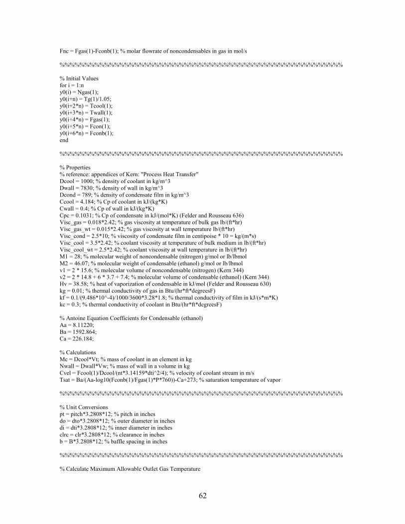
62

Fnc = Fgas(1)-Fconb(1); % molar flowrate of noncondensables in gas in mol/s %%%%%%%%%%%%%%%%%%%%%%%%%%%%%%%%%%%%%%%%%%%%%%%%%%%%%%%%% % Initial Values for i = 1:n y0(i) = Ngas(1); y0(i+n) = Tg(1)/1.05; y0(i+2*n) = Tcool(1); y0(i+3*n) = Twall(1); y0(i+4*n) = Fgas(1); y0(i+5*n) = Fcon(1); y0(i+6*n) = Fconb(1); end %%%%%%%%%%%%%%%%%%%%%%%%%%%%%%%%%%%%%%%%%%%%%%%%%%%%%%%%% % Properties % reference: appendices of Kern: "Process Heat Transfer" Dcool = 1000; % density of coolant in kg/m^3 Dwall = 7830; % density of wall in kg/m^3 Dcond = 789; % density of condensate film in kg/m^3 Ccool = 4.184; % Cp of coolant in kJ/(kg*K) Cwall = 0.4; % Cp of wall in kJ/(kg*K) Cpc = 0.1031; % Cp of condensate in kJ/(mol*K) (Felder and Rousseau 636) Visc_gas = 0.018*2.42; % gas viscosity at temperature of bulk gas lb/(ft*hr) Visc_gas_wt = 0.015*2.42; % gas viscosity at wall temperature lb/(ft*hr) Visc_cond = 2.5*10; % viscosity of condensate film in centipoise * 10 = kg/(m*s) Visc_cool = 3.5*2.42; % coolant viscosity at temperature of bulk medium in lb/(ft*hr) Visc_cool_wt = 2.5*2.42; % coolant viscosity at wall temperature in lb/(ft*hr) M1 = 28; % molecular weight of noncondensable (nitrogen) g/mol or lb/lbmol M2 = 46.07; % molecular weight of condensable (ethanol) g/mol or lb/lbmol v1 = 2 * 15.6; % molecular volume of noncondensable (nitrogen) (Kern 344) v2 = 2 * 14.8 + 6 * 3.7 + 7.4; % molecular volume of condensable (ethanol) (Kern 344) Hv = 38.58; % heat of vaporization of condensable in kJ/mol (Felder and Rousseau 630) kg = 0.01; % thermal conductivity of gas in Btu/(hr*ft*degreesF) kf = 0.1/(9.486*10^-4)/1000/3600*3.28*1.8; % thermal conductivity of film in kJ/(s*m*K) kc = 0.3; % thermal conductivity of coolant in Btu/(hr*ft*degreesF) % Antoine Equation Coefficients for Condensable (ethanol) Aa = 8.11220; Ba = 1592.864; Ca = 226.184; % Calculations Mc = Dcool*Vt; % mass of coolant in an element in kg Nwall = Dwall*Vw; % mass of wall in a volume in kg Cvel = Fcool(1)/Dcool/(nt*3.14159*dti^2/4); % velocity of coolant stream in m/s Tsat = Ba/(Aa-log10(Fconb(1)/Fgas(1)*P*760))-Ca+273; % saturation temperature of vapor %%%%%%%%%%%%%%%%%%%%%%%%%%%%%%%%%%%%%%%%%%%%%%%%%%%%%%%%% % Unit Conversions pt = pitch*3.2808*12; % pitch in inches do = dto*3.2808*12; % outer diameter in inches di = dti*3.2808*12; % inner diameter in inches clrc = clr*3.2808*12; % clearance in inches b = B*3.2808*12; % baffle spacing in inches %%%%%%%%%%%%%%%%%%%%%%%%%%%%%%%%%%%%%%%%%%%%%%%%%%%%%%%%% % Calculate Maximum Allowable Outlet Gas Temperature

63

% reference: EPA website: "State Implementation Plans: Illinois - Chicago Area VOC Rules - Pharmaceutical Manufacturing" Pconb = Fconb(1)/Fgas(1)*P*101.325; % inlet vapor pressure of condensable, kPa z = Tg(1)/293.4; % correction factor to operating temperature if Pconb >= 40*z Tg_max = 248.2; % maximum allowable outlet gas temperature in K elseif ((Pconb < 40*z)&(Pconb >= 20*z)) Tg_max = 258.2; elseif ((Pconb < 20*z)&(Pconb >= 10*z)) Tg_max = 273.2; elseif ((Pconb < 10*z)&(Pconb >= 7*z)) Tg_max = 283.2; elseif ((Pconb < 7*z)&(Pconb >= 3.45*z)) Tg_max = 298.2; else % fprintf('Outlet gas temperature not regulated. Specify maximum % value.') Tg_max = 298.2; end %%%%%%%%%%%%%%%%%%%%%%%%%%%%%%%%%%%%%%%%%%%%%%%%%%%%%%%%% % Calculate Heat Capacity of Gas Mixture % reference: Felder and Rousseau: "Elementary Principles of Chemical Processes" Table B.2 T = Tg(1) - 273; % T = initial temperature of gas in degrees Celsius % component 1 = nitrogen (noncondensable) % Cp nitrogen = a + b*T + c*T^2 + d*T^3 where T is in degrees C a1 = 29 * 10^-3; b1 = 0.2199 * 10^-5; c1 = 0.5723 * 10^-8; d1 = -2.871 * 10^-12; if T>0 % correlation valid for T > 0 degrees C Cp1 = a1 + b1*T + c1*T^2 + d1*T^3; % Cp of noncondensable in kJ/(mol*K) else Cp1 = a1; end Cp_1 = Cp1*1000*9.486*10^-4/1.8/M1*1000/2.2; % Cp of noncondensable in Btu/(lb*degF) % component 2 = ethanol (condensable) % Cp ethanol = a + b*T + c*T^2 + d*T^3 where T is in degrees C a2 = 61.34 * 10^-3; b2 = 15.72 * 10^-5; c2 = -8.749 * 10^-8; d2 = 19.83 * 10^-12; if T>0 Cp2 = a2 + b2*T + c2*T^2 + d2*T^3; % Cp of condensable in kJ/(mol*K) else Cp2 = a2; end Cp_2 = Cp2*1000*9.486*10^-4/1.8/M2*1000/2.2; % Cp of condensable in Btu/(lb*degF) % calculate Cpgas as a weighted average of the component Cps Cpgas = (Fnc/Fgas(1)) * Cp1 + (Fconb(1)/Fgas(1)) * Cp2; % kJ/(mol*K) Cp_gas = (Fnc*M1*Cp_1+Fconb(1)*M2*Cp_2)/(Fnc*M1+Fconb(1)*M2); % Btu/(lb*degF) %%%%%%%%%%%%%%%%%%%%%%%%%%%%%%%%%%%%%%%%%%%%%%%%%%%%%%%%% % Calculate Heat Transfer Coefficient for Gas

64

% reference: Kern: "Process Heat Transfer" p. 136-139 if pt == 1 de = 4*(pt^2-3.14159*do^2/4)/3.14159/do; % equivalent diameter in inches else de = 4*(0.5*pt*0.86*pt-0.5*3.14159*do^2/4)/(0.5*3.14159/do); end De = de/12; % equivalent diameter in feet Ag = di*clrc*b/pt/144; % flow area of gas in ft^2 Wg = (Fnc*M1+Fconb(1)*M2)/1000*2.2*3600; % mass flow rate of gas in lb/hr Ga = Wg/Ag; % mass flux of gas in lb/(hr*ft^2) Reg = De*Ga/Visc_gas; % Reynolds number for gas % hg = heat transfer coefficient for gas in Btu/(hr*ft^2*degreesF) for 2000 < Reg < 1,000,000 hg = 0.36 * Reg^0.55 * (Cp_gas*Visc_gas/kg)^(1/3)*(Visc_gas/Visc_gas_wt)^0.14*kg/De; hgas = hg/(9.486*10^-4)/1000/3600*(3.28^2)*1.8; % heat transfer coefficient for gas in kJ/(s*m^2*K) %%%%%%%%%%%%%%%%%%%%%%%%%%%%%%%%%%%%%%%%%%%%%%%%%%%%%%%%% % Calculate Heat Transfer Coefficient for Condensate Film % reference: Perry's Chemical Engineer's Handbook p. 5-20, 11-11 deltaT = Tsat-Twall(1); % temp difference between sat'd vapor and surface in K % h1film = heat transfer coefficient for film with 1 tube in kJ/(s*m^2*K) h1film = 0.73*kf/dto*((dto^3*Dcond^2*g*Hv)/(kf*Visc_cond*deltaT*M2/1000))^(1/4); nt2 = 2/3*nt1; % 2/3 of max number of tubes across diameter nt3 = int32(nt2); % truncate to integer value N = real(nt3); % convert to real number hfilm = h1film*N^(-1/4); % correction for multiple tubes, kJ/(s*m^2*K) %%%%%%%%%%%%%%%%%%%%%%%%%%%%%%%%%%%%%%%%%%%%%%%%%%%%%%%%% % Calculate Heat Transfer Coefficient for Coolant % reference: Kern: "Prosess Heat Transfer" p. 103-105 Ac = 3.14159*dti^2/4*3.2808^2; % flow area of coolant in ft^2 Wc = Fcool(1)/nt*3600*2.2; % mass flow rate of coolant per tube in lb/hr Gc = Wc/Ac; % mass flux of coolant per tube in lb/(hr*ft^2) Rec = dti*Gc/Visc_cool; % Reynolds number for coolant c = Ccool*1000*(9.486*10^-4)/2.2/1.8; % specific heat of cold fluid in Btu/(lb*degreesF) % hc = heat transfer coefficient for coolant in Btu/(hr*ft^2*degreesF) % note: eqs. valid for organic liquids, aqueous solutions, and gases, but not for water if Rec > 2100 hc = 0.027 * Rec^0.8 * (c*Visc_cool/kc)^(1/3)*(Visc_cool/Visc_cool_wt)^0.14*kc/dti; else hc = 1.86*(Rec*c*Visc_cool*dti/kc/L)^(1/3)*(Visc_cool/Visc_cool_wt)^0.14*kc/dti; end hcoolant = hc/(9.486*10^-4)/1000/3600*(3.28^2)*1.8; % heat transfer coefficient for coolant in kJ/(s*m^2*K) % correct to outer diameter of tube rather than inner diameter hcool = hcoolant*dti/dto; % heat transfer coefficient for coolant in kJ/(s*m^2/K) %%%%%%%%%%%%%%%%%%%%%%%%%%%%%%%%%%%%%%%%%%%%%%%%%%%%%%%%% % Calculate General Heat Transfer Coefficients alcool = hcool*A; % alpha for cooling fluid alg = 1/(1/hgas+1/hfilm)*A; % alpha for gas and film U = 1/(1/hgas + 1/hfilm + 1/hcool); % overall heat transfer coefficient kJ/(s*m^2*K) %%%%%%%%%%%%%%%%%%%%%%%%%%%%%%%%%%%%%%%%%%%%%%%%%%%%%%%%% % Calculate Diffusion Coefficient

65

% reference: Kern: "Process Heat Transfer" p. 343-344 % calculate diffusivity using Gilliland correlation kd = 0.0166 * (Tg(1))^(3/2)/ P / (v1^(1/3) + v2^(1/3))^2 * (1/M1 + 1/M2)^(1/2); % ft^2/hr KD = kd/3600/3.28^2; % diffusivity in m^2/s % calculate diffusion coefficient pg1 = (Fnc/Fgas(1))*P; % partial pressure of the inert gas in the gas body, atm pg2 = P-(10^(Aa-Ba/(Twall(1)-273+Ca)))/760; % partial pressure of the inert gas at the condensate film, atm pgf = (pg2-pg1)/log(pg2/pg1); % log mean pressure difference of the inert gas between pg1 and pg2, atm Mm = ((Fnc/Fgas(1))*M1 + (Fconb(1)/Fgas(1))*M2); % mean molecular weight of the vapor mixture, lb/lbmol Dgas = P*Mm/0.7302/(1.8*Tg(1)); % density of gas in lb/ft^3 % Kg = diffusion coefficient in lbmol/(hr*ft^2*atm) Kg = hg*((Cp_gas*Visc_gas/kg)^(2/3))/(Cp_gas*pgf*Mm*(Visc_gas/Dgas(1)/kd)^(2/3)); Dab = Kg*(3.2808^2)/3600*453.593; % diffusion coefficient in mol/(s*m^2*atm) %%%%%%%%%%%%%%%%%%%%%%%%%%%%%%%%%%%%%%%%%%%%%%%%%%%%%%%%% % Steady State Solution options0 = optimset('Display','iter','MaxFunEvals',1e5); [yss,fval,exitflag] = fsolve(@CondenserSS8b,y0,options0,Tg,Tcool,Twall,Fgas,Fcon,Fconb,Fnc,Fcool,A,alcool,Vs,P,R,Mc,Ccool,Cwall,Cpc,Nwall,Aa,Ba,Ca,Hv,n,alg,Cpgas,Dab); yss; yss(7*n+1) = 0; % set integral value Io = 0 % Plot Results PlotSS3b(yss,n,Aa,Ba,Ca,P,dz,Tg,Tcool,Twall,Fgas,Fcon,Fconb,alg,alcool,Hv,Cpc); % Extract Variables from Steady State Solution for i=1:n Ngas(i+1) = real(yss(i)); Tg(i+1) = real(yss(i+n)); Tcool(i+1) = real(yss(i+2*n)); Twall(i+1) = real(yss(i+3*n)); Fgas(i+1) = real(yss(i+4*n)); Fcon(i+1) = real(yss(i+5*n)); Fconb(i+1) = real(yss(i+6*n)); ygas(i+1) = Fconb(i+1)/Fgas(i+1); end % Error Calculations Input=(Fgas(1)); TotalCond=trapz(Fcon); FgasO=Fgas(n+1); FcondbO=Fconb(n+1); Accumulated=Vs*P*101325/(R*Tg(n+1)^2)*(Tg(1)-Tg(n+1)); Output=TotalCond+FgasO+Accumulated; Fconblein=Fconb(1); CAbsErr=Fconb(1)-TotalCond-FcondbO; CondbleError=(abs(CAbsErr))/(Fconb(1))*100; NonCondError=Fnc-(FgasO*(1-ygas(n+1))); %%%%%%%%%%%%%%%%%%%%%%%%%%%%%%%%%%%%%%%%%%%%%%%%%%%%%%%%% % Dynamic Solution kc = .1; Ti = 1.5; Tsp = Tg_max-5; % temperature set point in K tend = 240;

66

Mstep = tend/100; tspan = [0:tend]; % time horizon integrated nalg = 3; % number of algebraic eq ndiff = 4; % number of differential equations M = zeros((nalg+ndiff)*n:(nalg+ndiff)*n); % mass matrix for DAE for j=1:(ndiff)*n M(j,j) = 1; end M((ndiff+nalg)*n + 1, (ndiff+nalg)*n + 1) = 1; % control options = odeset('Mass',M,'Refine',5,'MaxStep',Mstep); [t,y] = ode15s(@CondenserDyn8b,tspan,yss,options,Tg,Tcool,Twall,Fgas,Fcon,Fconb,Fnc,Fcool,A,alcool,Vs,P,R,Mc,Ccool,Cwall,Cpc,Nwall,Aa,Ba,Ca,Hv,Ngas,n,alg,Cpgas,Dab,Tsp,kc,Ti); % Plot Results a = n; % length to be dispalyed in time PlotDynCond3(t,y,n,Aa,Ba,Ca,P,a,R,Vs); PlotDynError(t,y,n,Aa,Ba,Ca,P,a,R,Vs); PlotDynCondControl(t,y,n,Aa,Ba,Ca,P,a,R,Vs,Tsp,kc,Ti,Fcool); %%%%%%%%%%%%%%%%%%%%%%%%%%%%%%%%%%%%%%%%%%%%%%%%%%%%%%%%%

Steady State Solution: CondenserSS8b.m function [out] = CondenserSS8b(y,Tg,Tcool,Twall,Fgas,Fcon,Fconb,Fnc,Fcool,A,alcool,Vs,P,R,Mc,Ccool,Cwall,Cpc,Nwall,Aa,Ba,Ca,Hv,n,alg,Cpgas,Dab) % Variables Declaration for i=1:n Ngas(i+1) = real(y(i)); Tg(i+1) = real(y(i+n)); Tcool(i+1) = real(y(i+2*n)); Twall(i+1) = real(y(i+3*n)); Fgas(i+1) = real(y(i+4*n)); Fcon(i+1) = real(y(i+5*n)); Fconb(i+1) = real(y(i+6*n)); end %%%%%%%%%%%%%%%%%%%%%%%%%%%%%%%%%%%%%%%%%%%%%%%%%%%%%%%%% % System of Equations Declaration % Differential Equations for i=1:n % Mass Balance For Gas out(i)=Fgas(i)-Fgas(i+1)-Fcon(i+1); % Gas energy Balance out(i+n)=(Fgas(i)*Cpgas*(Tg(i)-Tg(i+1))-alg*(Tg(i+1)-Twall(i+1))-Fcon(i+1)*Hv)/(Ngas(i+1)*Cpgas); % Coolant energy Balance out(i+2*n)=(Fcool(1)*Ccool*(Tcool(i)-Tcool(i+1))+alcool*(Twall(i+1)-Tcool(i+1)))/(Mc*Ccool); % Wall energy Balance

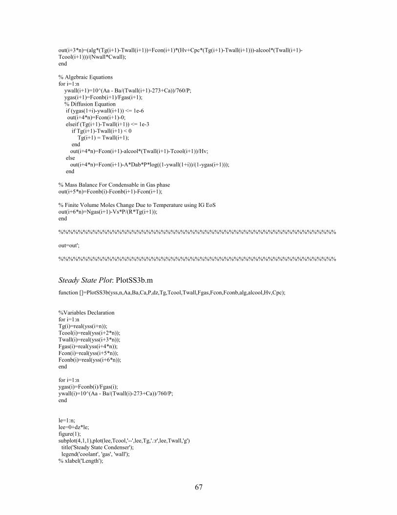
67

out(i+3*n)=(alg*(Tg(i+1)-Twall(i+1))+Fcon(i+1)*(Hv+Cpc*(Tg(i+1)-Twall(i+1)))-alcool*(Twall(i+1)-Tcool(i+1)))/(Nwall*Cwall); end % Algebraic Equations for i=1:n ywall(i+1)=10^(Aa - Ba/(Twall(i+1)-273+Ca))/760/P; ygas(i+1)=Fconb(i+1)/Fgas(i+1); % Diffusion Equation if (ygas(1+i)-ywall(i+1)) <= 1e-6 out(i+4*n)=Fcon(i+1)-0; elseif (Tg(i+1)-Twall(i+1)) <= 1e-3 if Tg(i+1)-Twall(i+1) < 0 Tg(i+1) = Twall(i+1); end out(i+4*n)=Fcon(i+1)-alcool*(Twall(i+1)-Tcool(i+1))/Hv; else out(i+4*n)=Fcon(i+1)-A*Dab*P*log((1-ywall(1+i))/(1-ygas(i+1))); end % Mass Balance For Condensable in Gas phase out(i+5*n)=Fconb(i)-Fconb(i+1)-Fcon(i+1); % Finite Volume Moles Change Due to Temperature using IG EoS out(i+6*n)=Ngas(i+1)-Vs*P/(R*Tg(i+1)); end %%%%%%%%%%%%%%%%%%%%%%%%%%%%%%%%%%%%%%%%%%%%%%%%%%%%%%%%% out=out'; %%%%%%%%%%%%%%%%%%%%%%%%%%%%%%%%%%%%%%%%%%%%%%%%%%%%%%%%%

Steady State Plot: PlotSS3b.m function []=PlotSS3b(yss,n,Aa,Ba,Ca,P,dz,Tg,Tcool,Twall,Fgas,Fcon,Fconb,alg,alcool,Hv,Cpc); %Variables Declaration for i=1:n Tg(i)=real(yss(i+n)); Tcool(i)=real(yss(i+2*n)); Twall(i)=real(yss(i+3*n)); Fgas(i)=real(yss(i+4*n)); Fcon(i)=real(yss(i+5*n)); Fconb(i)=real(yss(i+6*n)); end for i=1:n ygas(i)=Fconb(i)/Fgas(i); ywall(i)=10^(Aa - Ba/(Twall(i)-273+Ca))/760/P; end le=1:n; lee=0+dz*le; figure(1); subplot(4,1,1),plot(lee,Tcool,'--',lee,Tg,'.:r',lee,Twall,'g') title('Steady State Condenser'); legend('coolant', 'gas', 'wall'); % xlabel('Length');

68

ylabel('Temp (K)') subplot(4,1,2),plot(lee,ygas,'.:r',lee,ywall,'g') % title('Fg out vs L'); legend('gas', 'wall'); % xlabel('Time'); ylabel('VOC Conc. (mol fr.)') subplot(4,1,3),plot(lee,Fconb,'g') % title('Control vs time'); % xlabel('Length'); ylabel('Fconb (mol/s)') subplot(4,1,4),plot(lee,Fcon,'b') % title('Control vs time'); xlabel('Length (m)'); ylabel('Fcon (mol/s)') figure(2); qgas=alg*(Tg-Twall); qcond=Fcon.*(Hv+Cpc*(Tg-Twall)); qdisp=alcool*(Twall-Tcool); diff=qdisp-qgas; subplot(3,1,1),plot(lee,qgas) title('Steady State Condenser'); % xlabel('Length'); ylabel('Qgas (kJ/s)') subplot(3,1,2),plot(lee,qcond,lee,diff,'r.') % title('Fg out vs L'); % xlabel('Time'); ylabel('Qcond (kJ/s)') subplot(3,1,3),plot(lee,qdisp) % title('Control vs time'); xlabel('Length (m)'); ylabel('Qdisp (kJ/s)')

Dynamic Solution: CondenserDyn8b.m function [out] = CondenserDyn8b(t,y,Tg,Tcool,Twall,Fgas,Fcon,Fconb,Fnc,Fcool,A,alcool,Vs,P,R,Mc,Ccool,Cwall,Cpc,Nwall,Aa,Ba,Ca,Hv,Ngas,n,alg,Cpgas,Dab,Tsp,kc,Ti) % Variables Declaration for i=1:n Ngas(i+1) = real(y(i)); Tg(i+1) = real(y(i+n)); Tcool(i+1) = real(y(i+2*n)); Twall(i+1) = real(y(i+3*n)); Fgas(i+1) = real(y(i+4*n)); Fcon(i+1) = real(y(i+5*n)); Fconb(i+1) = real(y(i+6*n)); end I = real(y(7*n+1)); %%%%%%%%%%%%%%%%%%%%%%%%%%%%%%%%%%%%%%%%%%%%%%%%%%%%%%%%%

69

% Simulation Changes Tcool0 = Tcool(1); if t >= 120 Tcool(1) = 0.98*Tcool0; end %%%%%%%%%%%%%%%%%%%%%%%%%%%%%%%%%%%%%%%%%%%%%%%%%%%%%%%%% % System of Equations Declaration % Differential Equations for i=1:n % Mass Balance For Gas out(i)=-Vs*P/(R*(Tg(i+1))^2)*(Fgas(i)*Cpgas*(Tg(i)-Tg(i+1))-alg*(Tg(i+1)-Twall(i+1))-Fcon(i+1)*Hv)/(Ngas(i+1)*Cpgas); % Gas energy Balance out(i+n)=(Fgas(i)*Cpgas*(Tg(i)-Tg(i+1))-alg*(Tg(i+1)-Twall(i+1))-Fcon(i+1)*Hv)/(Ngas(i+1)*Cpgas); % Coolant energy Balance du = kc*(Tg(n+1)-Tsp+I); if (Fcool(1)+du) <= 1e-3 out(i+2*n)=(1e-3*Ccool*(Tcool(i)-Tcool(i+1))+alcool*(Twall(i+1)-Tcool(i+1)))/(Mc*Ccool); else out(i+2*n)=((Fcool(1)+du)*Ccool*(Tcool(i)-Tcool(i+1))+alcool*(Twall(i+1)-Tcool(i+1)))/(Mc*Ccool); end % Wall energy Balance out(i+3*n)=(alg*(Tg(i+1)-Twall(i+1))+Fcon(i+1)*(Hv+Cpc*(Tg(i+1)-Twall(i+1)))-alcool*(Twall(i+1)-Tcool(i+1)))/(Nwall*Cwall); end % Algebraic Equations for i=1:n ywall(i+1)=10^(Aa - Ba/(Twall(i+1)-273+Ca))/760/P; ygas(i+1)=Fconb(i+1)/Fgas(i+1); % Diffusion Equation if (ygas(i+1)-ywall(i+1)) <= 1e-6 out(i+4*n)=Fcon(i+1)-0; elseif (Tg(i+1)-Twall(i+1)) <= 1e-3 if Tg(i+1)-Twall(i+1) < 0 Tg(i+1) = Twall(i+1); end out(i+4*n)=Fcon(i+1)-alcool*(Twall(i+1)-Tcool(i+1))/Hv; else out(i+4*n)=Fcon(i+1)-A*Dab*P*log((1-ywall(1+i))/(1-ygas(i+1))); end % Mass Balance For Condensable in Gas phase out(i+5*n)=Fconb(i)-Fconb(i+1)-Fcon(i+1); % Finite Volume Moles Change Due to Temperature using IG EoS out(i+6*n)=Fgas(i)-Fgas(i+1)-Fcon(i+1)+Vs*P/(R*(Tg(i+1))^2)*(Fgas(i)*Cpgas*(Tg(i)-Tg(i+1))-alg*(Tg(i+1)-Twall(i+1))-Fcon(i+1)*Hv)/(Ngas(i+1)*Cpgas); end % Control out(7*n+1) = (Tg(n+1)-Tsp)*Ti; % dI/dt = e*Ti %%%%%%%%%%%%%%%%%%%%%%%%%%%%%%%%%%%%%%%%%%%%%%%%%%%%%%%%%

70

out = out'; %%%%%%%%%%%%%%%%%%%%%%%%%%%%%%%%%%%%%%%%%%%%%%%%%%%%%%%%%

Dynamic Plot 1: PlotDynCond3.m (See Dynamic Model Code)

Dynamic Plot 2: PlotDynError.m (See Dynamic Model Code)

Dynamic Controller Plot: PlotDynCondControl.m function []=PlotDynCondControl(t,y,n,Aa,Ba,Ca,P,a,R,Vs,Tsp,kc,Ti,Fcool) tfin = size(y); for i=1:tfin Ngas(i)=(y(i,a)); Tg(i)=(y(i,n+a)); Tcool(i)=(y(i,2*n+a)); Twall(i)=(y(i,3*n+a)); Fgas(i)=(y(i,4*n+a)); Fcon(i)=(y(i,5*n+a)); Fconb(i)=(y(i,6*n+a)); error(i) = Tg(i)-Tsp; I(i) = y(i,7*n+1); du(i) = kc*(error(i)+I(i)); Fcool_control(i) = Fcool(1)+du(i); end figure(5); subplot(2,2,1),plot(t,Tg,'.:r',t,Tcool,'--b',t,Twall,'g') title('Temporary reponse of element a') xlabel('Time (s)'); ylabel('Temp (K)'); legend('Gas', 'Coolant', 'Wall'); subplot(2,2,2),plot(t,Tg,'r') xlabel('Time (s)'); ylabel('Gas Temp (K)'); subplot(2,2,3),plot(t,error,'r') xlabel('Time (s)'); ylabel('Error (K)'); subplot(2,2,4),plot(t,Fcool_control,'b') xlabel('Time (s)'); ylabel('Coolant Flowrate (kg/s)');

71

APPENDIX VI: Steady State Uncertainty Evaluation

Independent Variation of One Variable (Cpgas, hgas, Dab constant) Data resulting from the independent variation of one variable in the steady state

model is shown in Table A6.1.

Table A6.1: Simulation Data for SS Uncertainty Evaluation: Independent Variation of One Variable (Cpgas, hgas, Dab constant with position)

Tg_in Tcool_in Fconb_in hgas Dab Tg_out Tcool_out Fconb_out Accum Error_C Error_NCNominal 350 230 15 0.1326 3.9935 266.37 234.23 9.56 0.912 0.491 0

345 230 15 0.1325 3.9744 261.85 234.15 9.58 0.938 0.489 7.11E-15346 230 15 0.1325 3.9782 262.75 234.17 9.57 0.933 0.490 -7.11E-15347 230 15 0.1325 3.9821 263.65 234.19 9.57 0.928 0.490 7.11E-15348 230 15 0.1326 3.9859 264.56 234.20 9.56 0.922 0.490 0

Change 349 230 15 0.1326 3.9897 265.46 234.22 9.56 0.917 0.490 0Tg_in 351 230 15 0.1327 3.9973 267.27 234.25 9.55 0.907 0.491 7.11E-15

352 230 15 0.1327 4.0011 268.17 234.26 9.55 0.902 0.491 7.11E-15353 230 15 0.1327 4.0049 269.08 234.28 9.54 0.897 0.491 7.11E-15354 230 15 0.1328 4.0087 269.98 234.30 9.54 0.892 0.492 -7.11E-15355 230 15 0.1328 4.0124 270.89 234.31 9.54 0.887 0.492 0350 228.0 15 0.1326 3.9935 266.08 232.26 9.55 0.917 0.491 0350 228.4 15 0.1326 3.9935 266.14 232.66 9.55 0.916 0.491 -7.11E-15350 228.8 15 0.1326 3.9935 266.19 233.05 9.55 0.915 0.491 0350 229.2 15 0.1326 3.9935 266.25 233.44 9.55 0.914 0.491 0

Change 350 229.6 15 0.1326 3.9935 266.31 233.84 9.55 0.913 0.491 0Tcool_in 350 230.4 15 0.1326 3.9935 266.42 234.63 9.56 0.911 0.491 7.11E-15

350 230.8 15 0.1326 3.9935 266.48 235.02 9.56 0.910 0.490 0350 231.2 15 0.1326 3.9935 266.54 235.42 9.56 0.909 0.490 -7.11E-15350 231.6 15 0.1326 3.9935 266.60 235.81 9.56 0.908 0.490 0350 232.0 15 0.1326 3.9935 266.66 236.20 9.56 0.907 0.490 -7.11E-15350 230 14.0 0.1317 3.9552 271.15 233.96 9.00 0.830 0.485 0350 230 14.2 0.1319 3.9628 270.20 234.01 9.11 0.846 0.486 0350 230 14.4 0.1321 3.9705 269.24 234.07 9.22 0.862 0.487 0350 230 14.6 0.1323 3.9781 268.29 234.12 9.33 0.878 0.488 0

Change 350 230 14.8 0.1325 3.9858 267.33 234.18 9.44 0.895 0.489 7.11E-15Fconb_in 350 230 15.2 0.1328 4.0013 265.40 234.29 9.67 0.929 0.492 -1.42E-14

350 230 15.4 0.1330 4.0090 264.43 234.34 9.78 0.947 0.493 0350 230 15.6 0.1332 4.0168 263.46 234.40 9.88 0.965 0.494 0350 230 15.8 0.1334 4.0247 262.48 234.45 9.99 0.983 0.496 0350 230 16.0 0.1335 4.0325 261.50 234.51 10.10 1.000 0.497 7.11E-15350 230 15 0.1061 3.1948 279.06 233.66 10.46 0.705 0.427 -7.11E-15350 230 15 0.1114 3.3545 276.41 233.78 10.27 0.745 0.441 7.11E-15350 230 15 0.1167 3.5143 273.83 233.90 10.09 0.786 0.454 0350 230 15 0.1220 3.6740 271.29 234.01 9.91 0.827 0.467 0

Change 350 230 15 0.1273 3.8338 268.80 234.13 9.73 0.869 0.479 -7.11E-15hgas 350 230 15 0.1379 4.1532 263.97 234.34 9.38 0.955 0.502 0

350 230 15 0.1432 4.3130 261.63 234.44 9.22 0.999 0.512 -7.11E-15350 230 15 0.1486 4.4727 259.33 234.54 9.05 1.040 0.522 7.11E-15350 230 15 0.1539 4.6325 257.07 234.63 8.89 1.090 0.531 -7.11E-15350 230 15 0.1592 4.7922 254.85 234.72 8.73 1.130 0.540 0350 230 15 0.1326 3.1948 278.50 233.68 10.46 0.713 0.427 0350 230 15 0.1326 3.3545 276.00 233.80 10.27 0.752 0.441 7.11E-15350 230 15 0.1326 3.5143 273.53 233.91 10.09 0.791 0.454 7.11E-15350 230 15 0.1326 3.6740 271.10 234.02 9.91 0.831 0.467 -7.11E-15

Change 350 230 15 0.1326 3.8338 268.72 234.13 9.73 0.871 0.479 0Dab 350 230 15 0.1326 4.1532 264.05 234.33 9.38 0.954 0.502 -7.11E-15

350 230 15 0.1326 4.3130 261.78 234.43 9.22 0.996 0.512 -7.11E-15350 230 15 0.1326 4.4727 259.54 234.53 9.05 1.040 0.522 -7.11E-15350 230 15 0.1326 4.6325 257.34 234.62 8.89 1.080 0.531 0350 230 15 0.1326 4.7922 255.17 234.71 8.73 1.130 0.540 7.11E-15

Steady State Condenser Model Uncertainty Evaluation: Independent Variation of One VariableCpgas, Hgas, Dab constant with position

Matlab files: SimCondenser_Eval_07_20_04.m, CondenserSS_Eval.m, PlotSS_Eval.m

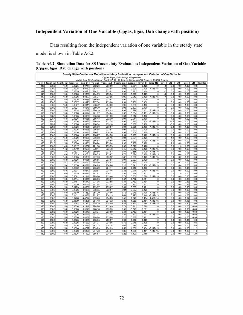
72

Independent Variation of One Variable (Cpgas, hgas, Dab change with position)

Data resulting from the independent variation of one variable in the steady state

model is shown in Table A6.2.

Table A6.2: Simulation Data for SS Uncertainty Evaluation: Independent Variation of One Variable (Cpgas, hgas, Dab change with position)

Tg_in Tcool_in Fconb_in hgas_in Dab_in Tg_out Tcool_out Fconb_out Accum Error_C Error_NC uf1 uf2 uf3 uf4 uf5 Exitflag345 230.0 15.0 0.1325 3.9744 262.26 233.89 9.96 0.931 0.428 0 -5 0.0 0.0 1.00 1.00 1346 230.0 15.0 0.1325 3.9782 263.14 233.91 9.96 0.926 0.428 7.11E-15 -4 0.0 0.0 1.00 1.00 1347 230.0 15.0 0.1325 3.9821 264.01 233.92 9.95 0.921 0.429 0 -3 0.0 0.0 1.00 1.00 1348 230.0 15.0 0.1326 3.9859 264.89 233.94 9.95 0.916 0.429 0 -2 0.0 0.0 1.00 1.00 1349 230.0 15.0 0.1326 3.9897 265.77 233.95 9.95 0.912 0.429 7.11E-15 -1 0.0 0.0 1.00 1.00 1350 230.0 15.0 0.1326 3.9935 266.65 233.97 9.94 0.907 0.429 0 0 0.0 0.0 1.00 1.00 1351 230.0 15.0 0.1327 3.9973 267.54 233.98 9.94 0.902 0.430 0 1 0.0 0.0 1.00 1.00 1352 230.0 15.0 0.1327 4.0011 268.42 234.00 9.93 0.898 0.430 0 2 0.0 0.0 1.00 1.00 1353 230.0 15.0 0.1327 4.0049 269.30 234.01 9.93 0.893 0.430 0 3 0.0 0.0 1.00 1.00 1354 230.0 15.0 0.1328 4.0087 270.19 234.03 9.93 0.888 0.431 7.11E-15 4 0.0 0.0 1.00 1.00 1355 230.0 15.0 0.1328 4.0124 271.07 234.04 9.92 0.884 0.431 -7.11E-15 5 0.0 0.0 1.00 1.00 1350 228.0 15.0 0.1326 3.9935 266.38 231.99 9.94 0.912 0.430 0 0 -2.0 0.0 1.00 1.00 1350 228.4 15.0 0.1326 3.9935 266.43 232.39 9.94 0.911 0.430 0 0 -1.6 0.0 1.00 1.00 1350 228.8 15.0 0.1326 3.9935 266.49 232.78 9.94 0.910 0.430 -7.11E-15 0 -1.2 0.0 1.00 1.00 1350 229.2 15.0 0.1326 3.9935 266.54 233.18 9.94 0.909 0.430 0 0 -0.8 0.0 1.00 1.00 1350 229.6 15.0 0.1326 3.9935 266.60 233.57 9.94 0.908 0.430 7.11E-15 0 -0.4 0.0 1.00 1.00 1350 230.0 15.0 0.1326 3.9935 266.65 233.97 9.94 0.907 0.429 0 0 0.0 0.0 1.00 1.00 1350 230.4 15.0 0.1326 3.9935 266.71 234.36 9.94 0.906 0.429 0 0 0.4 0.0 1.00 1.00 1350 230.8 15.0 0.1326 3.9935 266.77 234.76 9.94 0.905 0.429 7.11E-15 0 0.8 0.0 1.00 1.00 1350 231.2 15.0 0.1326 3.9935 266.83 235.15 9.94 0.904 0.429 0 0 1.2 0.0 1.00 1.00 1350 231.6 15.0 0.1326 3.9935 266.88 235.55 9.94 0.903 0.429 7.11E-15 0 1.6 0.0 1.00 1.00 1350 232.0 15.0 0.1326 3.9935 266.94 235.94 9.95 0.902 0.429 0 0 2.0 0.0 1.00 1.00 1350 230.0 14.0 0.1317 3.9552 271.38 233.73 9.33 0.826 0.428 0 0 0.0 -1.0 1.00 1.00 1350 230.0 14.2 0.1319 3.9628 270.44 233.78 9.45 0.842 0.428 7.11E-15 0 0.0 -0.8 1.00 1.00 1350 230.0 14.4 0.1321 3.9705 269.50 233.83 9.57 0.858 0.429 7.11E-15 0 0.0 -0.6 1.00 1.00 1350 230.0 14.6 0.1323 3.9781 268.55 233.87 9.70 0.874 0.429 7.11E-15 0 0.0 -0.4 1.00 1.00 1350 230.0 14.8 0.1325 3.9858 267.60 233.92 9.82 0.890 0.429 7.11E-15 0 0.0 -0.2 1.00 1.00 1350 230.0 15.0 0.1326 3.9935 266.65 233.97 9.94 0.907 0.429 0 0 0.0 0.0 1.00 1.00 1350 230.0 15.2 0.1328 4.0013 265.70 234.02 10.06 0.924 0.430 0 0 0.0 0.2 1.00 1.00 1350 230.0 15.4 0.1330 4.0090 264.75 234.06 10.18 0.941 0.430 -7.11E-15 0 0.0 0.4 1.00 1.00 1350 230.0 15.6 0.1332 4.0168 263.79 234.11 10.31 0.959 0.430 0 0 0.0 0.6 1.00 1.00 1350 230.0 15.8 0.1334 4.0247 262.84 234.16 10.43 0.976 0.431 7.11E-15 0 0.0 0.8 1.00 1.00 1350 230.0 16.0 0.1335 4.0325 261.87 234.21 10.55 0.994 0.431 0 0 0.0 1.0 1.00 1.00 1350 230.0 15.0 0.1061 3.1948 279.26 233.46 10.74 0.702 0.380 7.11E-15 0 0.0 0.0 0.80 1.00 1350 230.0 15.0 0.1114 3.3545 276.63 233.57 10.57 0.742 0.391 0 0 0.0 0.0 0.84 1.00 1350 230.0 15.0 0.1167 3.5143 274.06 233.68 10.41 0.782 0.401 0 0 0.0 0.0 0.88 1.00 1350 230.0 15.0 0.1220 3.6740 271.54 233.78 10.25 0.823 0.411 0 0 0.0 0.0 0.92 1.00 1350 230.0 15.0 0.1273 3.8338 269.07 233.87 10.09 0.865 0.421 0 0 0.0 0.0 0.96 1.00 1350 230.0 15.0 0.1326 3.9935 266.65 233.97 9.94 0.907 0.429 0 0 0.0 0.0 1.00 1.00 1350 230.0 15.0 0.1379 4.1532 264.29 234.06 9.79 0.949 0.438 -7.11E-15 0 0.0 0.0 1.04 1.00 1350 230.0 15.0 0.1432 4.3130 261.97 234.15 9.64 0.992 0.446 -7.11E-15 0 0.0 0.0 1.08 1.00 1350 230.0 15.0 0.1486 4.4727 259.70 234.23 9.50 1.040 0.454 1.42E-14 0 0.0 0.0 1.12 1.00 1350 230.0 15.0 0.1539 4.6325 257.48 234.32 9.36 1.080 0.461 7.11E-15 0 0.0 0.0 1.16 1.00 1350 230.0 15.0 0.1592 4.7922 255.29 234.40 9.22 1.120 0.468 7.11E-15 0 0.0 0.0 1.20 1.00 1350 230.0 15.0 0.1326 3.1948 278.66 233.49 10.74 0.711 0.380 0 0 0.0 0.0 1.00 0.80 1350 230.0 15.0 0.1326 3.3545 276.18 233.59 10.58 0.749 0.391 0 0 0.0 0.0 1.00 0.84 1350 230.0 15.0 0.1326 3.5143 273.74 233.69 10.41 0.787 0.401 0 0 0.0 0.0 1.00 0.88 1350 230.0 15.0 0.1326 3.6740 271.34 233.78 10.25 0.827 0.411 -7.11E-15 0 0.0 0.0 1.00 0.92 1350 230.0 15.0 0.1326 3.8338 268.98 233.88 10.10 0.867 0.421 0 0 0.0 0.0 1.00 0.96 1350 230.0 15.0 0.1326 3.9935 266.65 233.97 9.94 0.907 0.429 0 0 0.0 0.0 1.00 1.00 1350 230.0 15.0 0.1326 4.1532 264.37 234.06 9.79 0.948 0.438 0 0 0.0 0.0 1.00 1.04 1350 230.0 15.0 0.1326 4.3130 262.13 234.14 9.64 0.989 0.446 0 0 0.0 0.0 1.00 1.08 1350 230.0 15.0 0.1326 4.4727 259.93 234.23 9.50 1.030 0.454 -7.11E-15 0 0.0 0.0 1.00 1.12 1350 230.0 15.0 0.1326 4.6325 257.76 234.31 9.36 1.070 0.461 7.11E-15 0 0.0 0.0 1.00 1.16 1350 230.0 15.0 0.1326 4.7922 255.63 234.39 9.22 1.120 0.468 0 0 0.0 0.0 1.00 1.20 1

Steady State Condenser Model Uncertainty Evaluation: Independent Variation of One VariableCpgas, Hgas, Dab change with position

Matlab files: SimCondenser_Eval4_07_23_04_loop.m, CondenserSS_Eval4.m, PlotSS_Eval.m

73

Simultaneous Variation of Two Variables (Cpgas, hgas, Dab change with position)

Data from the simultaneous variation of two variables in the steady state model is

shown in Table A6.3.

Table A6.3: Simulation Data for SS Uncertainty Evaluation: Simultaneous Variation of Two Variables (Cpgas, hgas, Dab change with position)

Level Tg_in Tcool_in Fconb_in hgas_in Dab_in Tg_out Tcool_out Fconb_out Accum Error_C Error_NC uf1 uf2 uf3 uf4 uf5 Exitflag0 350 230.0 15.0 0.1326 3.9935 266.65 233.97 9.94 0.907 0.429 0 0 0.0 0.0 1.00 1.00 11 351 230.4 15.0 0.1327 3.9973 267.59 234.38 9.94 0.901 0.430 7.11E-15 1 0.4 0.0 1.00 1.00 12 352 230.8 15.0 0.1327 4.0011 268.53 234.79 9.93 0.896 0.430 7.11E-15 2 0.8 0.0 1.00 1.00 13 353 231.2 15.0 0.1327 4.0049 269.47 235.20 9.93 0.890 0.430 0 3 1.2 0.0 1.00 1.00 14 354 231.6 15.0 0.1328 4.0087 270.42 235.61 9.93 0.884 0.430 -7.11E-15 4 1.6 0.0 1.00 1.00 15 355 232.0 15.0 0.1328 4.0124 271.36 236.02 9.93 0.879 0.431 7.11E-15 5 2.0 0.0 1.00 1.00 10 350 230.0 15.0 0.1326 3.9935 266.65 233.97 9.94 0.907 0.429 0 0 0.0 0.0 1.00 1.00 11 351 230.0 14.8 0.1325 3.9896 268.49 233.94 9.82 0.886 0.429 0 1 0.0 -0.2 1.00 1.00 12 352 230.0 14.6 0.1323 3.9857 270.32 233.90 9.69 0.865 0.429 0 2 0.0 -0.4 1.00 1.00 13 353 230.0 14.4 0.1322 3.9818 272.15 233.87 9.56 0.845 0.429 7.11E-15 3 0.0 -0.6 1.00 1.00 14 354 230.0 14.2 0.1321 3.9779 273.97 233.84 9.44 0.825 0.429 0 4 0.0 -0.8 1.00 1.00 15 355 230.0 14.0 0.1319 3.9740 275.80 233.80 9.31 0.806 0.429 0 5 0.0 -1.0 1.00 1.00 10 350 230.0 15.0 0.1326 3.9935 266.65 233.97 9.94 0.907 0.429 0 0 0.0 0.0 1.00 1.00 11 350 230.4 14.8 0.1325 3.9858 267.66 234.32 9.82 0.889 0.429 0 0 0.4 -0.2 1.00 1.00 12 350 230.8 14.6 0.1323 3.9781 268.67 234.66 9.70 0.872 0.429 -7.11E-15 0 0.8 -0.4 1.00 1.00 13 350 231.2 14.4 0.1321 3.9705 269.67 235.01 9.58 0.855 0.428 7.11E-15 0 1.2 -0.6 1.00 1.00 14 350 231.6 14.2 0.1319 3.9628 270.67 235.36 9.45 0.838 0.428 -1.42E-14 0 1.6 -0.8 1.00 1.00 15 350 232.0 14.0 0.1317 3.9552 271.67 235.71 9.33 0.821 0.428 0 0 2.0 -1.0 1.00 1.00 10 350 230.0 15.0 0.1326 3.9935 266.65 233.97 9.94 0.907 0.429 0 0 0.0 0.0 1.00 1.00 11 350 230.0 15.0 0.1273 3.6804 271.34 233.78 10.25 0.827 0.412 -7.11E-15 0 0.0 0.0 0.96 0.96 12 350 230.0 15.0 0.1220 3.3801 276.00 233.60 10.55 0.752 0.393 0 0 0.0 0.0 0.92 0.92 13 350 230.0 15.0 0.1167 3.0926 280.61 233.41 10.85 0.682 0.373 0 0 0.0 0.0 0.88 0.88 14 350 230.0 15.0 0.1114 2.8178 285.16 233.21 11.15 0.617 0.352 0 0 0.0 0.0 0.84 0.84 15 350 230.0 15.0 0.1061 2.5558 289.64 233.02 11.45 0.557 0.330 0 0 0.0 0.0 0.80 0.80 10 350 230.0 15.0 0.1326 3.9935 266.65 233.97 9.94 0.907 0.429 0 0 0.0 0.0 1.00 1.00 11 351 230.0 15.0 0.1274 3.8374 269.96 233.89 10.09 0.860 0.421 0 1 0.0 0.0 0.96 1.00 12 352 230.0 15.0 0.1221 3.6810 273.31 233.81 10.24 0.815 0.412 -7.11E-15 2 0.0 0.0 0.92 1.00 13 353 230.0 15.0 0.1168 3.5243 276.73 233.72 10.40 0.771 0.402 0 3 0.0 0.0 0.88 1.00 14 354 230.0 15.0 0.1115 3.3673 280.21 233.63 10.56 0.727 0.392 -7.11E-15 4 0.0 0.0 0.84 1.00 15 355 230.0 15.0 0.1063 3.2099 283.74 233.53 10.72 0.685 0.381 7.11E-15 5 0.0 0.0 0.80 1.00 10 350 230.0 15.0 0.1326 3.9935 266.65 233.97 9.94 0.907 0.429 0 0 0.0 0.0 1.00 1.00 11 351 230.0 15.0 0.1327 3.8374 269.86 233.89 10.09 0.862 0.421 -1.42E-14 1 0.0 0.0 1.00 0.96 12 352 230.0 15.0 0.1327 3.6810 273.11 233.81 10.24 0.818 0.412 0 2 0.0 0.0 1.00 0.92 13 353 230.0 15.0 0.1327 3.5243 276.40 233.73 10.40 0.776 0.402 0 3 0.0 0.0 1.00 0.88 14 354 230.0 15.0 0.1328 3.3673 279.74 233.64 10.56 0.734 0.392 -7.11E-15 4 0.0 0.0 1.00 0.84 15 355 230.0 15.0 0.1328 3.2099 283.11 233.55 10.73 0.694 0.381 0 5 0.0 0.0 1.00 0.80 10 350 230.0 15.0 0.1326 3.9935 266.65 233.97 9.94 0.907 0.429 0 0 0.0 0.0 1.00 1.00 11 350 230.4 15.0 0.1273 3.8338 269.13 234.27 10.10 0.864 0.421 0 0 0.4 0.0 0.96 1.00 12 350 230.8 15.0 0.1220 3.6740 271.65 234.57 10.25 0.822 0.411 0 0 0.8 0.0 0.92 1.00 13 350 231.2 15.0 0.1167 3.5143 274.22 234.86 10.41 0.780 0.401 0 0 1.2 0.0 0.88 1.00 14 350 231.6 15.0 0.1114 3.3545 276.84 235.15 10.58 0.739 0.391 0 0 1.6 0.0 0.84 1.00 15 350 232.0 15.0 0.1061 3.1948 279.51 235.44 10.74 0.698 0.380 0 0 2.0 0.0 0.80 1.00 10 350 230.0 15.0 0.1326 3.9935 266.65 233.97 9.94 0.907 0.429 0 0 0.0 0.0 1.00 1.00 11 350 230.4 15.0 0.1326 3.8338 269.03 234.27 10.10 0.866 0.421 7.11E-15 0 0.4 0.0 1.00 0.96 12 350 230.8 15.0 0.1326 3.6740 271.45 234.57 10.25 0.825 0.411 0 0 0.8 0.0 1.00 0.92 13 350 231.2 15.0 0.1326 3.5143 273.90 234.87 10.41 0.785 0.401 -7.11E-15 0 1.2 0.0 1.00 0.88 14 350 231.6 15.0 0.1326 3.3545 276.40 235.17 10.58 0.745 0.391 0 0 1.6 0.0 1.00 0.84 15 350 232.0 15.0 0.1326 3.1948 278.93 235.46 10.75 0.707 0.380 0 0 2.0 0.0 1.00 0.80 10 350 230.0 15.0 0.1326 3.9935 266.65 233.97 9.94 0.907 0.429 0 0 0.0 0.0 1.00 1.00 11 350 230.0 14.8 0.1272 3.8264 269.99 233.83 9.97 0.849 0.420 0 0 0.0 -0.2 0.96 1.00 12 350 230.0 14.6 0.1217 3.6599 273.32 233.69 10.00 0.794 0.411 7.11E-15 0 0.0 -0.4 0.92 1.00 13 350 230.0 14.4 0.1162 3.4940 276.63 233.54 10.02 0.742 0.400 7.11E-15 0 0.0 -0.6 0.88 1.00 14 350 230.0 14.2 0.1108 3.3288 279.92 233.40 10.05 0.692 0.389 7.11E-15 0 0.0 -0.8 0.84 1.00 15 350 230.0 14.0 0.1054 3.1642 283.20 233.25 10.07 0.644 0.378 0 0 0.0 -1.0 0.80 1.00 10 350 230.0 15.0 0.1326 3.9935 266.65 233.97 9.94 0.907 0.429 0 0 0.0 0.0 1.00 1.00 11 350 230.0 14.8 0.1325 3.8264 269.89 233.83 9.97 0.851 0.420 7.11E-15 0 0.0 -0.2 1.00 0.96 12 350 230.0 14.6 0.1323 3.6599 273.11 233.69 10.00 0.798 0.410 -7.11E-15 0 0.0 -0.4 1.00 0.92 13 350 230.0 14.4 0.1321 3.4940 276.30 233.55 10.03 0.747 0.400 -7.11E-15 0 0.0 -0.6 1.00 0.88 14 350 230.0 14.2 0.1319 3.3288 279.45 233.41 10.05 0.699 0.389 0 0 0.0 -0.8 1.00 0.84 15 350 230.0 14.0 0.1317 3.1642 282.57 233.27 10.07 0.653 0.378 -7.11E-15 0 0.0 -1.0 1.00 0.80 1

Steady State Condenser Model Uncertainty Evaluation: Simultaneous Variation of Two VariablesCpgas, Hgas, Dab change with position

Matlab files: SimCondenser_Eval4_07_26_04_loop2.m, CondenserSS_Eval4.m, PlotSS_Eval.m