vo natural computation - uni salzburghelmut/teaching/naturalcomputation/handout.pdf · vo natural...
TRANSCRIPT

VO Natural Computation
VO Natural Computation
Helmut A. Mayer
Department of Computer SciencesUniversity of Salzburg
SS14
VO Natural Computation
Outline
Introduction
Genetics and Evolution
Global Optimization
Artificial EvolutionEvolution StrategiesEvolutionary ProgrammingGenetic AlgorithmsGenetic Programming
Biological Neural Networks
Artifical Neural Networks

VO Natural Computation
Introduction
Natural Computation
I Natural Computation is a branch of computer sciencesimulating the representation, processing and evolution ofinformation in biological systems on computers in order tosolve complex problems in science, business and engineering.
I ABSTRACT concepts from biology to computer science
I Methods and techniques are NOT limited by biology
I Applications are NOT limited to biology
I Biological sources of concepts

VO Natural Computation
Introduction
Natural Computation Models
I Evolution of Genotype → Adaptation of Phenotype
I Neural Information Processing as Computational Model
I Immune System, Swarms, Ants, Evolutionary Robotics, FuzzyReasoning, and much more . . .
I Literature
I Kevin Kelly, The New Biology of Machines, 1994I Richard Dawkins, The Blind Watchmaker, 1996I Gerald Edelman and Giulio Tononi, Consciousness, 2001

VO Natural Computation
Introduction
Overview EC
I Evolutionary Computation
I A glimpse at nature
I Global optimization
I Evolution Strategies, Genetic Algorithms, EvolutionaryProgramming, Genetic Programming

VO Natural Computation
Introduction
Overview ANN
I Artificial Neural Networks
I Biological Neural NetworksI ANN history: Hodgkin–Huxley, McCulloch–Pitts, Perceptron,
AdalineI Multi–Layer PerceptronsI ANN Training, Back–propagationI Kohonen’s Self Organizing MapI Recurrent Networks, Hopfield
VO Natural Computation
Introduction
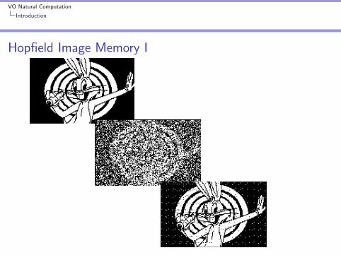
Hopfield Image Memory I

VO Natural Computation
Introduction
Hopfield Image Memory II

VO Natural Computation
Genetics and Evolution
Molecular Genetics
I DNA – DeoxyriboNucleinAcid Molecules, the codebook of lifeWatson & Crick ∼1960
I Adenosine (A), Thymidine (T ), Cytidine (C ), Guanosine (G )
I Basic Organisms
I Prokaryotes – viruses, bacteria, and blue–green algaeno discrete nucleus, no noncoding segments
I Eukaryotes – plants, animals, discrete nucleussubcellular compartments, noncoding segments
I Flow of Information = DNA → mRNA (Uracil for Thymidine)→ Ribosome, tRNA → Amino Acids → Protein
I Ribosome – Triplets, 43 = 64, but only 20 amino acids!
I Reading Frames, “Wobble Bases”

VO Natural Computation
Genetics and Evolution
Amino Acid Codons
First Base Second Base Third BaseU C A G
Phe Ser Tyr Cys UPhe Ser Tyr Cys CU Leu Ser STOP STOP ALeu Ser STOP Trp GLeu Pro His Arg ULeu Pro His Arg CC Leu Pro Gln Arg ALeu Pro Gln Arg GIle Thr Asn Ser UIle Thr Asn Ser CA Ile Thr Lys Arg A
Met START Thr Lys Arg GVal Ala Asp Gly UVal Ala Asp Gly CG Val Ala Glu Gly A
Val(Met) Ala Glu Gly G

VO Natural Computation
Genetics and Evolution
DNA Replication
I Enzyme splits duplex, Helicase unwinds, DNA Polymerase
I Replication fork moves with 800bp/s in E. Coli→ duplication in 40 minutes
I Eukaryotes 50bp/s, Mammalians ∼ 5× 10⁹bp/s → 1.5 yearsfor duplication → 90,000 replicons, massively parallel process
I Error rate = 10−6 for replication, 10−9 after proof reading

VO Natural Computation
Genetics and Evolution
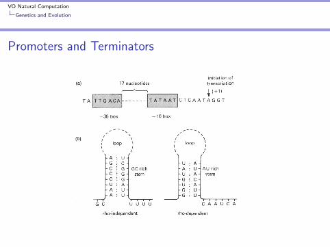
DNA Transcription
I Promoter/Terminator sequences + RNA Polymerase→ hnRNA (heterogenous nuclein) → spliced to mRNA
I Gene expression regulated by repressor/activator proteins
I Splicing = cutting out Introns, Alternative Splicing, ExonShuffling
I Introns Early vs. Introns Late Hypothesis
I E. Coli (4.6× 10⁶ bp → 3,000 proteins)Mammals (5× 10⁹ bp → 30,000 proteins)→ noncoding segments
VO Natural Computation
Genetics and Evolution
Promoters and Terminators
VO Natural Computation
Genetics and Evolution
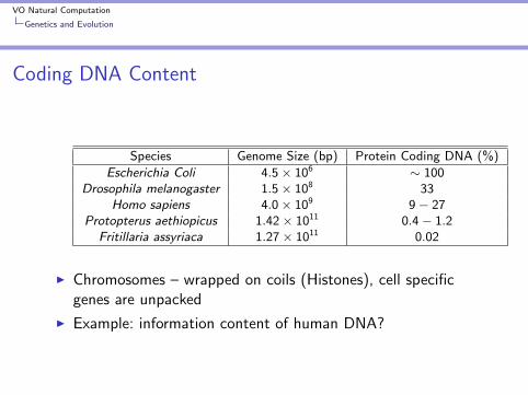
Coding DNA Content
Species Genome Size (bp) Protein Coding DNA (%)
Escherichia Coli 4.5× 10⁶ ∼ 100Drosophila melanogaster 1.5× 10⁸ 33
Homo sapiens 4.0× 10⁹ 9− 27Protopterus aethiopicus 1.42× 10¹¹ 0.4− 1.2
Fritillaria assyriaca 1.27× 10¹¹ 0.02
I Chromosomes – wrapped on coils (Histones), cell specificgenes are unpacked
I Example: information content of human DNA?

VO Natural Computation
Genetics and Evolution
Natural Evolution
I Lamarck (1744 – 1829): Inheritance of Acquired Traits
I Darwin (∼ 1860): Survival of the Fittest
I Selection due to limited resources, adaptation, niches
I Baldwin (1896): Phenotypical learning influences evolution ofgenotype (Baldwin Effect)
I Coevolution: “The evolution of a species is inseparable fromthe evolution of its environment. The two processes are tightlycoupled as a single indivisible process.” Lovelock 1988
I Central Dogma of Molecular Biology: Information only fromDNA to Protein

VO Natural Computation
Genetics and Evolution
Evolution Prerequisites
I Eigen (1970): Conditions for Darwinian Selection
I Metabolism, Self–Reproduction, and Mutation
I Mutation: new information
I Small error rates: slow progressLarge error rates: destroys information
I “Optimal” evolution: error rate just below destruction
I Literature
I Charles Darwin, On the Origin of Species, 1859I John Maynard Smith, Evolutionary Genetics, 1989

VO Natural Computation
Global Optimization
Optimization Definitions
I f : M ⊆ Rn → R,M 6= {},~x∗ ∈ M
I f ∗ := f (~x∗) > −∞ is a global minimum iff∀~x ∈ M : f (~x∗) ≤ f (~x) where
I ~x∗ . . . global minimum pointI f . . . objective functionI M . . . feasible region
I max{f (~x) | ~x ∈ M} = −min{−f (~x) | ~x ∈ M} . . . globalmaximum
I Constraints, Feasible Region
I M := {~x ∈ Rn | gi (~x) ≥ 0 ∀i ∈ {1 . . . q}}, gi : Rn → RI Satisfied constraint ⇔ gj(~x) ≥ 0I Active constraint ⇔ gj(~x) = 0I Inactive constraint ⇔ gj(~x) > 0I Violated constraint ⇔ gj(~x) < 0

VO Natural Computation
Global Optimization
TSP Problem
I Optimization problem example: Travelling Sales Person
I NP–complete, combinatorial, multimodal, CP–easy (CocktailParty easy;) D. Goldberg)
I C = {c1 . . . cn} . . . cities
I ρij = ρ(ci , cj) i , j ∈ {1 . . . n}, ρii = 0 . . . cost
I Π ∈ Sn = {s : {1 . . . n} → {1 . . . n}} . . . feasible tour
I f (Π) =∑n−1
i=1 ρΠ(i),Π(i+1) + ρΠ(n),Π(1) . . . objective function

VO Natural Computation
Global Optimization
Optimization Precautions
I In global optimization no general criterion for identification ofthe global optimum exists (Torn and Zilinskas 1990)
I No Free Lunch Theorem (NFL) “. . . all algorithms thatsearch for an extremum of a cost function perform exactlythe same, according to any performance measure, whenaveraged over all possible cost functions.” (Wolpert andMacready 1996)
VO Natural Computation
Artificial Evolution
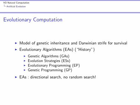
Evolutionary Computation
I Model of genetic inheritance and Darwinian strife for survival
I Evolutionary Algorithms (EAs) (“History”)
I Genetic Algorithms (GAs)I Evolution Strategies (ESs)I Evolutionary Programming (EP)I Genetic Programming (GP)
I EAs : directional search, no random search!

VO Natural Computation
Artificial Evolution
Application Criteria
I EAs are generic but not universal
I Optimization (broad class of problems)
I “Complex” problems (no conventional algorithm available)
I Features of candidate problems
I NP–complete problemsI High–dimensional search spaceI Non–differentiable surfaces (general absence of gradients)I Complex and noisy surfacesI Deceptive surfacesI Multimodal surfaces
VO Natural Computation
Artificial Evolution
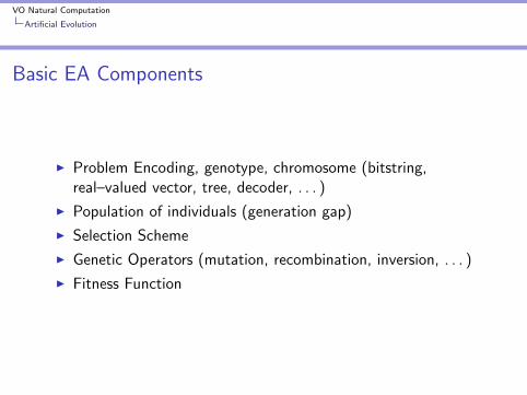
Basic EA Components
I Problem Encoding, genotype, chromosome (bitstring,real–valued vector, tree, decoder, . . . )
I Population of individuals (generation gap)
I Selection Scheme
I Genetic Operators (mutation, recombination, inversion, . . . )
I Fitness Function

VO Natural Computation
Artificial Evolution
Basic EA Pseudo–Code
A Basic Evolutionary Algorithm
BEGINgenerate initial populationWHILE NOT terminationCriterion DO
FOR populationSizecompute fitness of each individualselect individualsalter individuals
ENDFORENDWHILE
END

VO Natural Computation
Artificial Evolution
Evolution Strategies
Evolution Strategies Basics
I Bienert, Rechenberg, Schwefel: TU Berlin (1964)
I Chromosome: real valued vector
I Specific genetic operators and selection schemes
I Self–adaptation of mutation rate
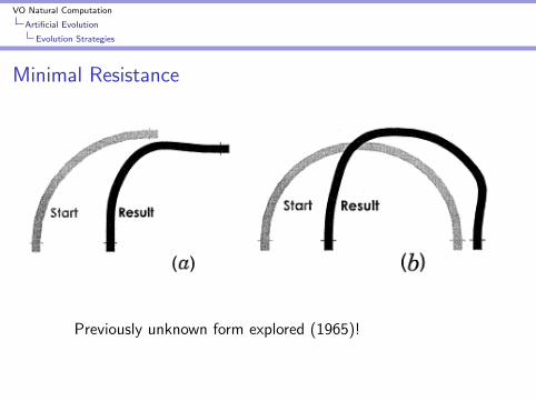
I First experiments: hydrodynamical problems (shapeoptimization of a bent pipe)

VO Natural Computation
Artificial Evolution
Evolution Strategies
Early Evolution Strategies
I Simple (1 + 1)–ES (population?)
I Object and strategy parameters
I Heuristic self–adaptation with 15 success rule
σ(t) =
σ(t − 1)c if p > 1
5σ(t − 1)/c if p < 1
5σ(t − 1) if p = 1
5
with c = n√
0.85
I Multi–membered ES, (µ+ λ), (µ, λ) selection
I Covariances (rotation angles)

VO Natural Computation
Artificial Evolution
Evolution Strategies
Self–adaptation
I n–dimensional normal distribution p(~z) = e−~zT C−1~z√
(2π)n|C |I Mutation of standard deviations σσ′i = σie
τ ′N(0,1)+τNi (0,1) with τ ′ ∼= 1√2n
and τ ∼= 1√2√n
I Mutation of rotation angles αα′j = αj + βNj(0, 1) with β ∼= 0.0837 ∼= 5o
I Mutation of object parameters xix ′i = x + ~N(~0,C (σi , αj))

VO Natural Computation
Artificial Evolution
Evolution Strategies
Recombination
I Recombination, discrete, intermediate, local, global
x ′i =
xS ,ixS ,i ∨ xT ,ixS ,i + u(xT ,i − xS ,i )xSi ,i ∨ xTi ,ixSi ,i + ui (xTi ,i − xSi ,i )
S ,T random parent individuals
I Empiric: object parameters (discrete recombination)strategy parameters (intermediate recombination)

VO Natural Computation
Artificial Evolution
Evolution Strategies
ES History
I First experiments 1964, TU Berlin
I Pictures from: Ingo Rechenberg, Evolutionsstrategie ’94(1994)
I Further literatureI Hans–Paul Schwefel, Evolution and Optimum Seeking, (1995)I Thomas Back, Evolutionary Algorithms in Theory and
Practice, (1996)

VO Natural Computation
Artificial Evolution
Evolution Strategies
Plate Resistance

VO Natural Computation
Artificial Evolution
Evolution Strategies
Pipe Resistance Experiment
VO Natural Computation
Artificial Evolution
Evolution Strategies
Minimal Resistance
Previously unknown form explored (1965)!

VO Natural Computation
Artificial Evolution
Evolutionary Programming
Evolutionary Programming Basics
I No recombination!
I Additional mutation κ when mapping genotype to phenotype
I Genotype (object parameters) mutationx ′i = xi + Ni (0, 1)
√βi f (~x) + γi (standard βi = 1 and γi = 0)
I Meta–EP, self–adaptation
I EP selection: every individual scores on q randomly chosencompetitors, EP selection → (µ+ µ) ES selection
I Literature
I L. J. Fogel and A. J. Owens and M. J. Walsh, ArtificialIntelligence through Simulated Evolution (1966)
I D. B. Fogel, System Identification through SimulatedEvolution: A Machine Learning Approach to Modeling, (1991)

VO Natural Computation
Artificial Evolution
Genetic Algorithms
Genetic Algorithm BasicsI John Holland, Ann Arbor, Michigan (1960s)I Chromosome: fixed length bit strings
bi ∈ {0, 1} i ∈ {1, . . . l}I One–point crossover and bit–flip mutation
A Basic Genetic Algorithm
BEGINgenerate initial populationWHILE NOT terminationCriterion DO
FOR populationSizecompute fitness of each individualrecord overall best individualselect individuals to mating poolrecombine and mutate individuals
ENDFORnew generation replaces old
ENDWHILEoutput overall best individualEND
I Encoding of solutions, e.g., real valuesx = c + d−c
2l−1
∑li=1 bi2
i−1, genotype I = {b1, . . . bl},phenotype x ∈ [c , d ]

VO Natural Computation
Artificial Evolution
Genetic Algorithms
Genetic Operators
I Crossover is main GA operator(?)
I k–point, uniform, problem specific, crossover probabilitypc∼= [0.6− 0.8]
I Mutation background operator(?)
I Reintroduction of lost materialI Mutation probability pm
∼= [0.01− 0.001]I Theory pm = 1
l , analogue to nature(!)

VO Natural Computation
Artificial Evolution
Genetic Algorithms
Fitness Function Design
I Keep it simple, no artificial measures
I Invalid solutions, refine operators or use penalty
I Penalty Functions
I “Death Penalty”I Fixed PenaltyI Dynamic PenaltyI Measure of obstruction (no simple count of obstructions)

VO Natural Computation
Artificial Evolution
Genetic Algorithms
Knapsack Problem
I Encoding example
I Set of items gi , i = 1, . . . , n
I Each item has a price pi and a weight wi
I Select items (put into knapsack){gk |
∑m≤nk=1 pk → max ∧
∑m≤nk=1 wk ≤ wmax}
I Encoding? Fitness Function?
I Incorporate problem knowledge, usually GA + Heuristics >GA (prevents however unconventional solutions)

VO Natural Computation
Artificial Evolution
Genetic Algorithms
Selection Methods
I Fitness proportionate selection
I Roulette Wheel selection (sampling methods)ps,i = fi∑n
i=1 fi, i ∈ {1, . . . ,N}
I Scaling methods, e.g., Sigma Scalingfbase = f − gσf , g ∈ Rf ′i = fi − fbase
I Rank based selection
I Linear Ranking, Exponential Rankingps,i = f (r), r ∈ {1, . . . , n}
I Tournament Selectiontournament size ⇔ selection pressure
I Truncation Selection

VO Natural Computation
Artificial Evolution
Genetic Algorithms
GA Analysis Definitions
I Schemata, e.g. 1 ∗ ∗ ∗ ∗ ∗ ∗∗ and ∗01 ∗ ∗ ∗ ∗1 (length l = 8)
I Schema Orderσ =| {i | bi ∈ {0, 1} | σ1 = 1, σ2 = 3
I Defining Lengthδ = max{i | bi ∈ {0, 1}} −min{i | bi ∈ {0, 1}}, δ1 = 0, δ2 = 6
VO Natural Computation
Artificial Evolution
Genetic Algorithms
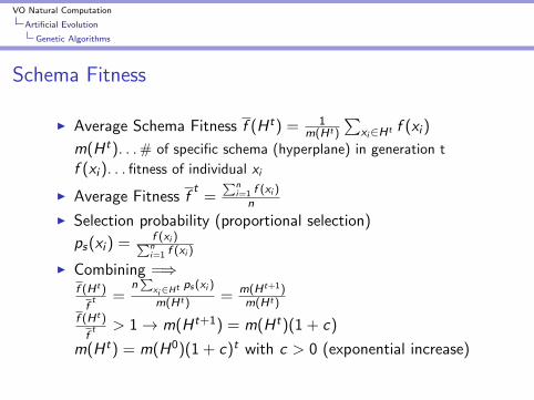
Schema Fitness
I Average Schema Fitness f (Ht) = 1m(Ht)
∑xi∈Ht f (xi )
m(Ht). . . # of specific schema (hyperplane) in generation t
f (xi ). . . fitness of individual xi
I Average Fitness ft
=∑n
i=1 f (xi )n
I Selection probability (proportional selection)
ps(xi ) = f (xi )∑ni=1 f (xi )
I Combining =⇒f (Ht)
ft =
n∑
xi∈Ht ps(xi )
m(Ht) = m(Ht+1)m(Ht)
f (Ht)
ft > 1→ m(Ht+1) = m(Ht)(1 + c)
m(Ht) = m(H0)(1 + c)t with c > 0 (exponential increase)

VO Natural Computation
Artificial Evolution
Genetic Algorithms
Schema Theorem
I Schema survival probability under 1–point crossover
1− pcδ(Ht)l−1
I Schema survival probability under mutation(1− pm)σ(Ht)
I Fundamental Theorem of GAsm(Ht+1) ≥ m(Ht) f (Ht)
ft (1− pc
δ(Ht)l−1 )(1− pm)σ(Ht)
I ST flaws: finite population sizes, generalization of singlegeneration transition, proportional selection. . .
I Building Block Hypothesis: Short, low–order, and highly fitschemata are sampled, recombined, and resampled to formstrings of potentially higher fitness. (Goldberg, 1989)
I Implicit Parallelism: O (n3) schemata are processed“simultaneously“

VO Natural Computation
Artificial Evolution
Genetic Algorithms
K–Armed Bandit
I Exploration–Exploitation model
I k = 2, N trials, 2n exploration trials, payoffs (µ1, σ1), (µ2, σ2)Expected loss L(N, n) = |µ1 − µ2|[(N − n)q(n) + n(1− q(n))]q(n) . . . probability that worse arm is observed best arm
I Minimizing L→ n∗ (optimal experiment size)N ∼ en
∗, exponentially increase trials to the oberved best arm
I GA analogue
I k schemata with ‘*’ at identical loci ↔ k–armed banditI all schemata ↔ multiple k–armed bandit problemI optimal strategy ↔ Schema Theorem

VO Natural Computation
Artificial Evolution
Genetic Algorithms
Literature
I John Holland, Adaptation in Natural and Artificial Systems(1975)
I David Goldberg, Genetic Algorithms in Search, Optimization& Machine Learning (1989)
I Zbigniew Michalewicz, Genetic Algorithms + Data Structures= Evolution Programs (1992)
I Melanie Mitchell, An Introduction to Genetic Algorithms(1996)

VO Natural Computation
Artificial Evolution
Genetic Programming
Genetic Programming Basics
I John Koza, Stanford (1988)
I Evolution of hierarchical computer programs
I Why use LISP?
I Programs and data are S–expressionsI LISP program is its own parse treeI EVAL function starts programI Dynamic storage allocation and garbage collection
I GP today: Assembler, C, Java

VO Natural Computation
Artificial Evolution
Genetic Programming
GP Design I
I Function set F and terminal set T , e.g.,F = {AND,OR,NOT}T = {D0,D1}C = F ∪ T
I Closure of C , protected functions, e.g.,(defun srt(argument)
‘‘The Protected Square Root Funtion’’
(sqrt (abs argument)))
I Sufficiency of C , problem knowledge
I Initial structures, maximum tree depthfull, grow, ramped half–and–half

VO Natural Computation
Artificial Evolution
Genetic Programming
GP Design II
I Fitness function
I Raw fitness rr(i , t) =
∑Nj=1 |S(i , j)− C (j)|
N . . . fitness casesS(i , j) . . . program valueC (j) . . . correct value
I Standardized fitness ss(i , t) = r(i , t) or s(i , t) = rmax − r(i , t)
I Adjusted fitness aa(i , t) = 1
1+s(i,t)I Normalized fitness n
n(i , t) = a(i,t)∑nk=1 a(k,t)

VO Natural Computation
Artificial Evolution
Genetic Programming
GP Design III
I GP population sizes (1,000 - 10,000)
I Proportionate selection
I Primary GP operator is crossover
I Secondary GP operators
I Mutation, random subtree insertionI Permutation (of arguments)I Editing, e.g., (NOT (NOT X)) → XI Encapsulation, “freezing of subtrees”I Decimation (esp. initial population)
I Literature
I John R. Koza, On the Programming of Computers by meansof Artificial Intelligence (1992)

VO Natural Computation
Artificial Evolution
Genetic Programming
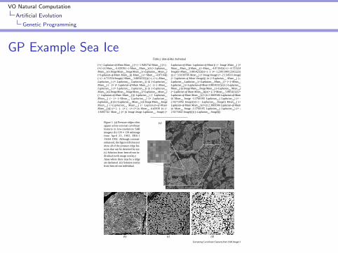
GP Example
I Daida et al., Extracting Curvilinear Features from SyntheticAperture Radar Images of Arctic Ice: Algorithm DiscoveryUsing the Genetic Programming Paradigm, IGARS 1995
I Classification of Radar ImagesI Sea Ice Analysis, Pressure RidgesI Evolved code generates good results but...
VO Natural Computation
Artificial Evolution
Genetic Programming
GP Example Sea Ice
Extracting Curvilinear Features from SAR Images 3
(÷ (+ Laplacian-of-Mean Mean3×3
) (÷ (+ 1.9492742 Mean3×3
) (× (–(× (÷ (≤ Mean
5×5 -4.42039 (– (–Mean
3×3 Mean
3×3) (≤ (+ Laplacian
5×5
Mean3×3
) (≤ Image Mean5×5
Image Mean5×5
) (÷Laplacian5×5
Mean3×3
)(÷Laplacian-of-Mean Mean
5×5))) Mean
5×5) (÷ Mean
3×3 -4.87104))
(÷ (÷ -4.721524 Image) (÷Mean5×5
3.8854232))) (÷ (– (÷ (–Mean3×3
Laplacian5×5
) (× Laplacian5×5
Laplacian5×5
)) (≤ (+Laplacian5×5
Mean3×3
) (– (× (× Laplacian-of-Mean Mean3×3
) (– (÷ (–Mean3×3
Laplacian5×5
) (× Laplacian5×5
Laplacian5×5
)) (≤ (+Laplacian5×5
Mean3×3
) (≤ Image Mean5×5
Image Mean5×5
) (÷Laplacian5×5
Mean3×3
)(÷ Laplacian-of-Mean Mean
5×5)))) Laplacian
5×5) (÷ Laplacian
5×5
Mean3×3
) (– (÷ (–Mean3×3
Laplacian5×5
) (× Laplacian5×5
Laplacian5×5
)) (≤ (+Laplacian5×5
Mean3×3
) (≤ Image Mean5×5
ImageMean
5×5) (÷Laplacian
5×5 Mean
3×3) (÷ Laplacian-of-Mean
Mean5×5
))))) (÷ (– (– (× (– (× (÷ (≤ Mean5×5
4.42039 (≤ (+1.9492742 Mean
3×3) (× (≤ Image Image Laplacian
5×5 Image) (+
Laplacian-of-Mean Laplacian-of-Mean)) (+ Image Mean3×3
) (×Mean
5×5 Mean
5×5)) Mean
5×5) (÷ Mean
3×3 -4.87104)) (÷ (÷ -4.721524
Image) (÷Mean5×5
3.8854232))) (÷ (– (– (× -1.2301508 0.2565225)(≤ (+ 3.6199708 Mean
3×3) (÷ Image Image) (÷ -2.134516 Image)
(+ Laplacian-of-Mean Image))) (≤ (+Laplacian5×5
Mean3×3
) (–Laplacian
5×5 Laplacian
5×5) (÷Laplacian
5×5 Mean
3×3) (– (÷ (–Mean
3×3
Laplacian5×5
) (÷ Laplacian-of-Mean 3.8854232)) (≤ (+Laplacian5×5
Mean3×3
) (≤ Image Mean5×5
Image Mean5×5
) (÷Laplacian5×5
Mean3×3
)(÷ Laplacian-of-Mean Mean
5×5))))) (÷ (– (÷Mean
5×5 3.8854232) (÷
Laplacian-of-Mean Mean3×3
)) (× (≤ 2.3869586 Laplacian-of-Mean(≤ Mean
3×3 Image -3.3760195 Laplacian
5×5) Laplacian
5×5) (÷ -
2.9275842 Image))))) (– Laplacian5×5
Image)) Mean5×5
) (÷Laplacian-of-Mean Mean
3×3)) (× (≤ 2.3869586 Laplacian-of-Mean
(≤ Mean3×3
Image -3.3760195 Laplacian5×5
) Laplacian5×5
) (÷ -2.9275842 Image))))) (–Laplacian
5×5 Image))))
Table 2. Best-of-Run Individual
(a)Figure 1. (a) Pressure ridges oftenappear as low-contrast curvilinearfeatures in low-resolution SARimagery. (b) 128 × 128 subimagefrom April 23, 1992, ERS-1©ESA 1992. Although contrast-enhanced, the figure still does notshow all of the pressure ridge fea-tures that can be detected by eye.(c) Solution from best-of-run in-dividual (with image overlay.)Areas where there may be a ridgeare darkened. (d) Solution (only)from best-of-run individual.
(b) (c) (d)

VO Natural Computation
Biological Neural Networks
Biological Neurons
I Nervous System: Control by Communication
I Massive Parallelism, Redundancy, Stochastic “Devices”
I Humans: 1010 neurons, 1014 connections (conservativeestimation), 101,000,000 possible networks(!)
I Neurons: cell body (soma), axon, synapses, dendrites
I Membrane Potential of −70mVsodium (Na+) and potassium (Ka+) ions (chloride Cl− ions)
I Sodium pump constantly expells Na+ ions
I Complex interaction of membrane, concentration, andelectrical potential

VO Natural Computation
Biological Neural Networks
Schematic Neuron
Synapses
Dendrites
Axon
SomaNucleus

VO Natural Computation
Biological Neural Networks
Electrical Signals
I Potassium is in equilibrium, sodium NOT
I Sodium conductance is a function of the membrane potential
I Above threshold sodium conductance increases, ion channels,depolarization, polarization, refractory period = actionpotential
I Frequency coding, is (all) information encoded in actionpotentials?
I Hodgkin/Huxley–Model

VO Natural Computation
Biological Neural Networks
Action Potential (from en.wikipedia.org)
VO Natural Computation
Biological Neural Networks
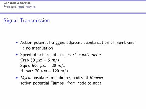
Signal Transmission
I Action potential triggers adjacent depolarization of membrane→ no attenuation
I Speed of action potential ∼√
axondiameterCrab 30 µm − 5 m/sSquid 500 µm − 20 m/sHuman 20 µm − 120 m/s
I Myelin insulates membrane, nodes of Ranvieraction potential “jumps” from node to node

VO Natural Computation
Biological Neural Networks
Synapses I
I Electrochemical processes, neurotransmitters
I Connect axon–dendrites (but also axon–axon,dendrites–dendrites, synapses–synapses)
I Spatio–temporal integration of action potentials
I Excitatory and inhibitory potentialspostsynaptic duration ∼ 5 ms
I Neurotransmitters influence threshold (permanent changes =learning = closing/opening of ion channels)

VO Natural Computation
Biological Neural Networks
Synapses II
I Slow Potential Theory: Spike frequency codes potential,Vf–converter
I Noise: ionic channels, synaptic vesicles (storeneurotransmitter), postsynaptic frequency estimation (in∼100ms a frequency range from 1–100Hz)
I BNN great variety of synapses, ANN mostly one type of“synapse”

VO Natural Computation
Artifical Neural Networks
Neuron Models
I Level of Simplification?
I McCulloch and Pitts (1943), Logic ModelBinary signals, no weights, simple (nonbinary) thresholdExcitatory and inhibitory connections (absolute, relative)Addition of weights
I Rosenblatt (1958), PerceptronReal–valued weights and threshold
VO Natural Computation
Artifical Neural Networks
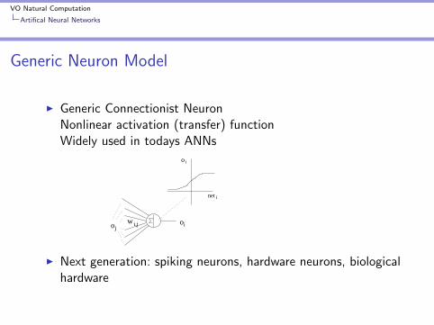
Generic Neuron Model
I Generic Connectionist NeuronNonlinear activation (transfer) functionWidely used in todays ANNs
net
o i
i
i,jojoiw
I Next generation: spiking neurons, hardware neurons, biologicalhardware

VO Natural Computation
Artifical Neural Networks
Networks
I Mysticism of Neural Networks
I Functional Model: f : Rn → Rm
node structure, connectivity, learn algorithm
I “Black Box Syndrom”, unexplicable ANN decisions
I Basic Structures: Feed–Forward (MLPs, Kohonen),f = f (g(x))Recurrent (Recurrent MLPs, Hopfield),f = f (xt , f (xt−1), f (xt−2), . . .)

VO Natural Computation
Artifical Neural Networks
ANN Training
I ANN Training (Learning, Teaching): Adjustment of networkparameters
I General Training Methods
I Supervised Learning (Teacher, I/O–Patterns)I Reinforcement Learning (Teacher, Learn Signal)I Unsupervised Learning (No Teacher, Self–Organization)

VO Natural Computation
Artifical Neural Networks
ANN Application Domains
I Constraint Satisfaction (Scheduling, n–Queens)
I Content Addressable Memory (Image Retrieval)
I Control (Machines, “ANN Driver”)
I Data Compression
I Diagnostics (Medicine, Production)
I Forecasting (Financial Markets, Weather)
I General Mapping (Function Approximation)
I Multi Sensor Data Fusion (Remote Sensing)
I Optimization
I Pattern Recognition (Voice, Image)
I Risk Assessment (Credit Card)

VO Natural Computation
Artifical Neural Networks
Perceptron
I Rosenblatt: Perceptron = Retina + A(ssociation) Layer +R(esponse) Layer, Retina → A (partial connections), A ↔ R(recurrent connections), Threshold Logic Unit (TLU)
I Simplified Perceptron is easier to analyze
I Weight and input vectors, scalar product, threshold as weight
I Linear SeparabilityTwo sets of points A and B in an n–dimensional space arelinearly separable, if there exist n + 1 real numbersw1, . . . ,wn+1 so that for each point x = (x1, . . . , xn) ∈ A:∑n
i=1 wixi ≥ wn+1
and for each point x = (x1, . . . , xn) ∈ B:∑ni=1 wixi < wn+1
I Standard Perceptron demands linearly separable problems

VO Natural Computation
Artifical Neural Networks
Perceptron Learning
I Perceptron Learn AlgorithmStart: Random ~w0, t := 0
Test: Random ~x ∈ P ∪ N
If ~x ∈ P and ~wt~x > 0⇒ TestIf ~x ∈ N and ~wt~x < 0⇒ TestIf ~x ∈ P and ~wt~x ≤ 0⇒ AddIf ~x ∈ N and ~wt~x ≥ 0⇒ Sub
Add: ~wt+1 := ~wt +~xSub: ~wt+1 := ~wt −~x
t := t + 1Exit if no weight update ∀~x
I Perceptron Convergence Theorem
I “Attack” on perceptrons: M. Minsky and S. PapertPerceptrons (1969)
I The XOR–function of two boolean variables x1, x2 cannot becomputed with a single perceptron. (Connectedness)

VO Natural Computation
Artifical Neural Networks
Earlier Models
I Hebbian Learning, Donald Hebb (1949)“When an axon of cell A is near enough to excite a cell B andrepeatedly or persistently takes part in firing it, some growthprocess or metabolic change takes place in one or both cellssuch that A’s efficiency as one of the cells firing B isincreased.”
I Generalized Hebb Rule∆wi ,j = η ai bj
I Linear Associator, input vector ~a, output vector ~bW = η~b~aT
I ADALINE (Adaptive Linear Element), Widrow and Hoff(1960)Threshold, error signal, error function has single minimumlearning rule is special case of backpropagation

VO Natural Computation
Artifical Neural Networks
Gradient Descent
I Basic Optimization Method
I How to compute the steepest descent? → Gradient
I The Nabla Operator (3 dimensions) ~∇ =
∂∂x∂∂y∂∂z
I Total Differential of E (x , y , z): dE = ∂E
∂x dx + ∂E∂y dy + ∂E
∂z dz
I Differential Path Element ~ds =
dxdydz
I Gradient ~gradE = ~∇E
I dE = ~gradE ~ds → maximal, if ~gradE || ~ds
I Note: div~E = ~∇~E (Divergence), rot~E = ~∇× ~E (Curl)

VO Natural Computation
Artifical Neural Networks
Widrow–Hoff Learning Rule
k,jwzyj
t
Ik
k
k
I Gradient Descent, ∆wk,j = −η ∂E∂wk,j
I Error E =∑P
p=1 E (p), E (p) =∑m
k=1 (t(p)k − I
(p)k )2
I p training patterns, m output neurons, t . . . target value
I ∂E (p)
∂wk,j= ∂
∂wk,j(∑m
k=1 (t(p)k −
∑hj=1 wk,jy
(p)j )2) =
= −2(t(p)k − I
(p)k )y
(p)j
I Omitting pattern index p∆wk,j = η(tk − Ik)yj = ηδkyj

VO Natural Computation
Artifical Neural Networks
Multi–Layer Perceptron
I Learning as minimization (of network error)
I Error is a function of network parameters
I Gradient descent methods reduce error
I Problem with perceptrons with hidden layers
I Backpropagation = Iterative Local Gradient DescentWerbos (1974), Rumelhart, Hinton, Williams (1986)
I Error–Backpropagation, output error is transmitted backwardsas weighted error, network weights are updated locally
I Weight update ∆wj ,i = ηδjaiGeneralized error term δ
I Common transfer functions: differentiable, nonlinear,monotonous, easily computable differentiation

VO Natural Computation
Artifical Neural Networks
Error–Backpropagation Ix1
x2
H1
H2
I1
I2 z2
z1
y1
y2
w12
w22
w21
w11v11
v21
v12
v22
I Hj =∑n
i=1 vj ,ixi Ik =∑h
j=1 wk,jyjyj = f (Hj), zk = f (Ik)
I Error E (p) = 12
∑mk=1 (t
(p)k − z
(p)k )2
I Output Layer: ∆wk,j = −η ∂E∂wk,j
∂E∂wk,j
= ∂E∂Ik
∂Ik∂wk,j
= ∂E∂Ik
yj∂E∂Ik
= ∂E∂zk
∂zk∂Ik
= −(tk − zk)f ′(Ik)∂E∂wk,j
= −(tk − zk)f ′(Ik)yj mit δk = (tk − zk)f ′(Ik)
∆wk,j = ηδkyj

VO Natural Computation
Artifical Neural Networks
Error–Backpropagation II
I Hidden Layer: ∆vj ,i = −η ∂E∂vj,i
∂E∂vj,i
= ∂E∂Hj
∂Hj
∂vj,i= ∂E
∂Hjxi
∂E∂Hj
= ∂E∂yj
∂yj∂Hj
= ∂E∂yj
f ′(Hj)
∂E∂yj
= −12
∑mk=1
∂(tk−f (Ik ))2
∂yj= −
∑mk=1 (tk − zk)f ′(Ik)wk,j
mit δj = f ′(Hj)∑m
k=1 δkwk,j
∆vj ,i = ηδjxiI Local update rules propagating error from output to input
I Present all p patterns of the training set = 1 Epoch (completetraining e.g., 1,000 epochs)
I Batch Learning (Off–line): accumulate weight changes for allpatterns, then update weights
I On–line Learning: update weights after each pattern

VO Natural Computation
Artifical Neural Networks
Backpropagation Variants I
I Standard Backpropagation: ~wt = ~wt−1 − η~∇E
I Gradient Reuse: use ~∇E as long as error drops
I BP with variable stepsize (learn rate) η
I BP with momentum: ∆ ~wt = −η~∇E + α∆ ~wt−1

VO Natural Computation
Artifical Neural Networks
Backpropagation Variants II
I Rprop (Resilient Backpropagation), Riedmiller/Braun, 1993
∆wi ,j(t) =
−∆i ,j(t) if ∂E
∂wi,j> 0
+∆i ,j(t) if ∂E∂wi,j
< 0
0 else
∆i ,j(t) =
{η+∆i ,j(t − 1) if ∂E(t−1)
∂wi,j× ∂E(t)
∂wi,j> 0
η−∆i ,j(t − 1) if ∂E(t−1)∂wi,j
× ∂E(t)∂wi,j
< 0
0 < η− < 1 < η+
I Second order methodsE (~w) = E ( ~wt)+(~w− ~wt)~∇E ( ~wt)+ 1
2 (~w− ~wt)H(~w− ~wt)T +. . .
~∇E (~w) = ~∇E ( ~wt) + (~w − ~wt)H → ~∇E (~w) = ~0Hessian Matrix H, complex computations, nonlocalinformations!

VO Natural Computation
Artifical Neural Networks
Self Organizing MapsI Cerebral Cortex: topologically ordered maps (sensory inputs)I Willshaw and von der Malsburg (1976)
two layers, intra–connections (short-range excitatory,long-range inhibitory), inter–connections (Hebbian learning)
I Kohonen (1982)Topological map, vector quantization, competitive learning
wj,i
xi
hj,i
xI
Abbildung: A two–dimensional self organizing map.

VO Natural Computation
Artifical Neural Networks
SOM Formation
I SOM Learning
I Competition: input triggers winner–takes–allI Cooperation: identify topological neighborhoodI Synaptic Adaptation: enhance response of winner and
neighbors
I Competition, input ~x , weight ~wj , winneri(~x) = arg minj |~x − ~wj |
I Cooperation, output neuron position ~ri , neigborhood hj ,i(~x)
dj ,i = |~rj −~ri | hj ,i(~x) = e−d2
j,i
2σ(t)2 σ(t) = σ0e−tτ1
I Adaptation
∆~wj = η(t)hj ,i(~x)(t)(~x − ~wj(t)) η(t) = η0e−tτ2

VO Natural Computation
Artifical Neural Networks
SOM Properties
I Approximation of input space, topological ordering
I Density matching, nonlinear principal components (PCA)
Abbildung: SOM formation of unit square topology (fromwww.learnartificialneuralnetworks.com)
.