VM577P: Capital Management and Investment Decisions

Ownership Costs, Capital Budgeting and Investing (the Cliff’s Notes Version)

Draft 2.12 JM Gay DVM PhD DACVPM 12/15

On-line version - http://www.vetmed.wsu.edu/courses-jmgay/documents/VM577OwnershipCosts.pdf

Warning: Not being a qualified tax advisor, financial planner or certified accountant, I provide this to acquaint you with the basic terms and concepts associated with borrowing, investing, capital budgeting and ownership costs. Seek advice from qualified professionals before making major financial decisions or transactions, such as purchasing a practice. Although I took engineering, MBA, and grad school classes in this many years ago, I admit to not using the information nor to following my advice. If you spot errors or points needing clarification, please let me know. No endorsements are intended or implied in the following.

Note: This handout is intended for veterinary students intending to enter agricultural animal practice and for practitioners in that professional segment.

Introduction

The independently wealthy satisfy their want for the newest digital technology, big green machines, new vehicles and high value replacement stock irrespective of return from that capital investment. For the rest of us, to justify a business investment we need a reasonable expectation of recovering the capital investment, ownership, and operating costs, whether it is a Utrecht fetotome, a fiberoptic scope, an ultrasound, a practice vehicle, advanced training for a specialized procedure or developing a new client service. To remain in business, a business must generate sufficient cash over the short run to meet its immediate obligations (liquidity), such as paying salaries, and a sufficient return on investment over the long run (solvency) to justify its continued existence. Although many purchase equipment and make other investments, such as in themselves, with little more than the hope that things will turn out okay, the following is useful for reducing uncertainty and putting numbers on hope.

Because businesses use these methods frequently, many books are available and the internet has everything from background information to spreadsheets to on-line calculators to on-line courses. With the caveat that locations change frequently and that I’ve not assessed their content for accuracy, I’ve embedded URL’s as entry points to further information and provided more in the additional information section.

Axioms of Finance: (modified with apologies to AJ Keown et al.)

1. Cash is King – Because net cash from profits are what a business reinvests, cash flows rather than accounting profits measure value. Liquidity is key when “stuff happens (SHTF),” such as a severe economic downturn. Accounting “profits” are susceptible to jiggery-pokery for making recent numbers look good to part the naive from their money

2. Understanding the time value of money (TVM) is key – A dollar received or spent today is worth more than a dollar received or spent in the future. As part of their intertemporal choice to delay consumption, people expect compensation for using (borrowing) their dollar today

3. Compounding grows exponentially – What is beneficial for lenders is painful for borrowers; starting money growing sooner pays off for investors and stopping it from growing sooner pays off for

borrowers. Using the Rule of 72, the approximate doubling time of an investment in years is 72 / % interest rate and the halving time for a dollar in value is approximately 72 / % inflation rate.

4. The risk-return tradeoff – Most financial decisions require evaluating an uncertain risk-return tradeoff involving the future and we won’t undertake additional risks of future loss unless we expect to receive additional future compensation. Generally we don’t weigh monetarily equivalent risks and benefits logically, being loss adverse (prospect theory, behavioral economics).

5. Risks are not equal - Some risks can be mitigated and some not, predicting risk is difficult, and informed diversification reduces risk. Insurance protects against the risk of a major catastrophe by averaging (pooling) the cost across similar at-risk entities, a larger proportion at high risk increasing the cost to the pool and a larger proportion at low risk decreasing the cost.

6. Incremental cash flows –Only those cash flows that would change because of the decision count in the analysis of the decision

7. Efficient capital markets –Markets are quick and, in the aggregate over time, the prices are right (providing access and trading costs are low, supply and demand information is readily available, many traders are in the marketplace, the rule of law holds, business practice standards are enforced and the economy is stable). Financial markets exist because people use borrowing and lending to adjust their consumption over time (intertemporal choices).

8. The curse/benefit of competitive markets – Profits in excess of their risk premium don’t exist long because competition moves in to exploit the gap or disruptive innovation occurs, requiring either product/service differentiation or cost reduction to remain competitive. Whether competitive markets are a curse or a benefit depends on whether you are a seller or a buyer

9. Taxes complicate decisions – taxes complicate personal and business financial decisions 10. The agency dilemma – People have difficulty acting in the best interests of others unless their interests

are directly aligned or they have an explicit fiduciary responsibility under the law. To work in your best interest, individuals need “skin in the game” that aligns their interests with yours. Because professionals (e.g. lawyers, accountants, brokers) cannot fairly represent the opposing interests of both parties involved in a transaction, having them do so is likely penny-wise and pound-foolish for one of the parties. The interests of real estate, insurance, lending, broker, and manufacturers agents are often in conflict with yours and the law does not require them to fully disclose these conflicts. Independent insurance brokers and financial planners are often paid commissions for the products they market to you, a fact that they are not required by law to disclose. Employees who have a stake in a business beyond a salary are more likely to act in ways more favorable toward that business.

11. Ethics are challenging - ethical behavior is doing the right thing, ethical dilemmas are everywhere in business, and determining what is right and what is wrong beyond fiduciary duties established in the law is difficult

12. You get more of what you measure / acknowledge / reward – Incentives matter. Transparency and feedback reduce the agency problem. Individual responses often aren’t rational, depending on framing.

13. The 50% employee salary–cost gap An employee’s direct cost to a business ~1.25 x their salary and they net ~0.75 of that salary, the ~50% gap between what they cost the business and their net pay going to government.

14. Plan, plan – Without a plan fewer good things happen over the long term; get started planning and then implementing the plan sooner rather than later but don’t fall victim to analysis paralysis.

15. Aphorisms:

• “Don’t put all your eggs in one basket” – Diversifying is a basic strategy for mitigating risk, whether investing in the stock market, the bond market, or forming a family

• “There’s no such thing as free lunch” – “free” things have strings attached somewhere, some how. Always! Violations of the basic laws and principles only occur in the short term and never without compensation in the long term

• “If it sounds too good to be true, it is” – Often what appears to be magic is sleight of hand. Avoid mistakes born from greed. If it was such a good deal, strangers likely wouldn’t be offering it to you or your friends because they wouldn’t need your money nor need it so quickly. Knowledge of typical risks and typical returns is the best protection. The long run return to money from low risk investment is 3 to 4% over inflation with considerable random variation in the near term. Forgetting or not knowing this and playing to greed enables Ponzi schemes such as Bernie Madoff's and accounting scandals such as Enron and WorldCom to occur.

• “Compound interest is man’s greatest invention” (often erroneously attributed to Einstein) – Eliminate debt and begin investing ASAP.

• “Price is what you pay. Value is what you get” (Warren Buffett) • “Investing is simple, but not easy” (Warren Buffett - ?) • “Never invest in a business you can’t understand” (Warren Buffet - ?)

Background

Due to unavoidable uncertainty about future business factors, both business-specific (e.g., value of a service to clientele, demand for a service) and the external business environment (e.g., interest rates, regulatory changes, tax law changes, and economic trends and events), investment and ownership decisions are complicated. For example, is investing in the specialized equipment and training to provide a particular service likely to pay off and, if so, how soon? How much of the service will clients consume at a price that you can afford to provide it? For seasonal services, how much capacity is optimal? When will advancing technology and standards of practice likely make current equipment obsolete or disrupt demand? What level of technology is sufficient? Should you buy two smaller ones or one big one? Should you buy new (higher depreciation, lower repair costs, newer technology) or buy or fix used (lower depreciation, higher repair costs, older technology)? Laser printers cost more than inkjet printers but have lower operating (per page) costs. When is the best time to trade your current practice vehicle on a new one? Trade-in decisions are complex because rising expected repair costs with use (high mileage or tachometer hours) offset declining ownership costs due to the length of ownership (unit is fully depreciated) compared to the ownership and operating costs of a new or used replacement unit. Although newer technology may have lower operating costs, how well is its reliability known?

Some costs and benefits are intangible, money is only the way of keeping score of some of the tangible, and there is more to life than money. Larger pickups cost more but may be safer in crashes than smaller ones. A clean crew-cab pickup can haul the family more comfortably than a conventional cab. An aged pickup is more likely to leave you a-foot in the middle of nowhere in the middle of the night than a new one but it is likely easier and often cheaper to fix when it does. Brand new or flashy equipment and old or beat-up equipment present a different image to your clients than does modest, up-to-date, well-maintained equipment. Having your office in a business building costs more than having your office in your home. The former one reduces family interruptions (clients assume that because you are there already, you won’t mind the Sunday interruption) while the other increases family time (your kids can at least watch you do book work even if you

aren’t giving them your full attention). Per The E-Myth Revisited, a separate business is easier to work on than in, an important distinction.

Your business goal is to allocate your scarce resources (time, money) to those activities with the best prospects for the best returns, whether in your business or outside of it. Business management includes these decisions. Finance is establishing asset worth and managing money flows (funds), particularly investing and financing (“debt”), between the business and financial firms (e.g., banks, stock brokerages, lenders). Managerial or corporate finance is the business component. Accounting (“bookkeeping”) is the method for keeping track and occurs in several forms. Tax accounting is required for settling up with you silent business partner, Uncle Sam, and is the main reason small business owners use accountants. For tax purposes, agricultural producers often use cash accounting rather than accrual-basis (double-entry) accounting, the latter giving a more accurate financial picture of the business. Because equipment purchasing and expensing options have tax implications, consult a certified public accountant before purchasing major items. Financial accounting provides a structured outline of how the business has and will make money. It tracks debits and credits of historical business transactions, such as between the practice and its clients (accounts receivable), its suppliers (accounts payable) and its financial intermediaries (e.g., banks, stock brokers, lenders), and produces financial statements (e.g., balance sheet, cash flow statement, income statement) and financial ratios (e.g., liquidity, solvency, profitability and turnover ratios) for evaluating general business health. Lenders often require historical and pro forma (projections based on assumptions) versions of these statements. Because this information is used by stakeholders outside the business who have legal recourse, these reports usually follow Generally Accepted Accounting Principles (GAAP). Managerial, management or cost accounting is used internally to determine, track and allocate the future within business costs of doing business, and to project the cost of goods sold or services provided. Because this information is used within the business (the business owners can only fool themselves), standards are not established. Capital budgeting is that component of managerial accounting dealing with equipment and project investments with cash flows expected to occur over more than one year. Examples are decisions about whether you should purchase one or the other in the first place, which of two services you should provide, whether you should expand or contract a service, whether you should buy or lease, when you should sell or replace equipment, and the minimum you need to recover per year or per procedure to recover your equipment costs.

Due to opportunity, interest, inflation, and risk, the value of money changes with time such that a dollar in hand today (present value) is worth more than a dollar tomorrow (future value). For making comparisons, basic financial mathematical TVM (time value of money) formulas are used to adjust future time effects to a common baseline time point, usually the present. The calculations can be performed by hand using tables, with financial calculators, with on-line applets, and with spreadsheet financial models. For the purposes of identifying good textbooks, these methods fall within the farm management component of agricultural economics, the capital budgeting component of financial modeling and are the whole of engineering economics (economy).

Although the mathematics are straightforward, omitting or double counting a cash flow or including a pseudo-cash flow may lead to decision-altering mistakes. Having several verified examples of analyses that resemble your decision situation is wise. Achieving the same results from entering these numbers into your spreadsheet model or several on-line calculators verifies that you are doing the analysis correctly, that you can mimic their analysis process for your situation and that the tool is performing correctly in that instance. Be careful; many

spreadsheets (and likely on-line calculators and publications) contain serious errors (Powell, Baker and Lawson, 2008) and many examples are simplified for instructional purposes.

The power of spreadsheet models is the ease of performing sensitivity analysis and “what if?” scenario analyses. What happens if inflation rises rapidly? If fuel price triples? If clients consume only half of the amount of service you are projecting? What is the benefit from adding a technician to increase throughput (e.g., cows/hour)? Understanding the consequences of uncertainty is important because single estimates imply misleading precision and small changes in critical variables may have big effects. The worst case scenario consequences may be so severe (e.g., bankruptcy) that the investment risk exceeds your risk tolerance for undertaking it even though the average scenario is profitable.

Base the amount you charge on the value of the service to your client, not on your cost of providing the service. If clients value a service less than your cost of providing it, you have four choices. Either reduce your costs in the value chain, acknowledge that your other services are subsidizing this service, exit this service market, or change client perception of its value. Marketing is the process of ensuring that clients understand the value proposition of your service, particularly if they are likely to underestimate its economic value to them. (For more, see “HPM – Veterinary Marketing and Salesmanship” – pdf)

Asides

Agricultural producers face similar decisions. Larger tractors pull larger implements than smaller tractors, covering ground quicker so that field operations are more timely and the labor cost per acre is less. On the other hand, the initial investment is larger and the fuel costs per hour are higher when the larger tractor is used for tasks that a smaller tractor could do equally well. Newer tractors are less likely to breakdown than older ones. Breakdowns at critical times reduce yields and crop value but trading too soon increases ownership costs. Below what production level is replacing a mature cow with an un-proven heifer economically beneficial? Veterinary recommendations to producers often involve equipment and facility investments that have ownership and operating costs, such as changing feed mixing equipment to improve consumption, upgrading milking machines to improve udder health, or changing cattle handling facilities to improve safety.

Just as livestock operations are comprised of related enterprises (e.g., forage production, replacement rearing, mature herd production unit) that should be analyzed on their own merits, you will make better decisions if you analyze the enterprises within a veterinary practice on their own merits. For example, when considering building a clinic, considering it as a real estate enterprise may lead to constructing a less expensive but more general purpose commercial building that generates a higher return on investment than a special purpose, higher cost building because it is more flexible, more saleable and less impacted by obsolescence.

Business ownership provides the opportunity to shield personal income by including as business expenses for tax purposes items that are only indirectly business-related. For example, if you use your practice truck to pull a fishing boat 400 miles to hot fishing spots every free weekend during the fishing season, you can likely split the ownership and operating costs with your partner, Uncle Sam, by not breaking out vehicle operating expense. However, for business management you will make better decisions and have a stronger business if you allocate truck expenses more in accordance with its actual usage. On the other hand, if your business is structured as a sole proprietorship or partnership your personal and business net worth are commingled, which complicates your financial decisions. Should you pay down your student debt or invest in equipment, both of which have different tax consequences? Managing a partnership over the long haul is difficult, leading to the old adage that “partnerships are the only ships that don’t float.” In contrast to sole proprietorships and

partnerships, forming a limited liability company (LLC) or incorporating places a firewall between your business and your family, limiting business financial obligations and legal liabilities to the business.

These methods are applicable to personal financial decisions, such as borrowing and spending now vs. saving and spending later, choosing the best saving options for future expenses such as a child’s college tuition, selecting the best loan instrument, determining if you should refinance a home mortgage, evaluating the effect of using a home equity line of credit in place of consumer debt, the benefit from consolidating loans, and so on. Because the first responsibility of lenders and real estate agents is to the seller, not to you as a borrower or buyer, you at least need to know the right questions to ask, such as what is the net present value of this loan with all the costs included. For more information on mortgages, see “The Mortgage Professor’s website.” Because compounded returns compound upon themselves, “paying yourself first” by investing a percentage of your income when you have any (or allowing debt interest to compound) is a must. Many personal finance experts suggest investing at least 10%, some as much as 15%, of your personal gross income, first maximizing any employer-match in a 401K plan, the maximum contribution to a Roth IRA and the balance in an un-matched 401K plan. Pay attention to handling fees when making personal investments; what seems like a small percentage has a huge impact in the end. (See Bogle JC (2005). The relentless rules of humble arithmetic. Financial Analysts J 61(6):22-35).

Key Concepts and their Definitions:

Capital budgeting: the process of identifying and selecting capital investment opportunities

Capital investment: Long term assets. The business’s investment in capital assets, which are generally tangible and intangible assets that have an economic life longer than a year such as land, buildings, facility, vehicles, major medical equipment

Working capital: Short term assets, accounts receivable, cash on hand. Money invested in inventory, such as pharmaceuticals, minor repair parts, and disposable items that are expected to be used up and replaced within a year.

Capital “project”: the set of investments contingent upon each other, such as new equipment, facility modifications, additional training, and increased working capital (e.g., expanded inventory of drugs and disposables), required for providing a new service (or producing a product)

Project types:

• New service that requires purchasing equipment or diverting of existing equipment or other resources, such as professional labor, from their current use, which incurs the opportunity cost of doing something else less

• Expansion of a current service that requires reallocation of scarce resources, such as professional time

• Replacement of an equipment item (e.g., current practice truck, imaging machine) that changes costs but does not affect revenues

• Investment mandated by a regulatory agency, such as OSAH, EPA or a state agency

Project dependence:

• Independent – cash flows including are not related to any other project and thus have no opportunity costs, which is a rare situation

• Mutually exclusive – acceptance of one precludes the acceptance of another • Contingent – project cannot occur without the undertaking of another • Complementary – investment in one increases the cash flows of another

Costs are two general types, fixed or variable:

Fixed costs: Remain relatively constant whether the equipment sits on shelf, is used some or a lot, and little or a lot of business is done over the time period.

Overhead costs: Fixed costs of doing business (e.g., liability insurance, utilities, building depreciation, property taxes, accounting fees, receptionist salary) that are incurred. Because they are not uniquely associated with a specific service or procedure, they are apportioned across services or procedures on some arbitrary basis.

Salary thumb rule - an employee typically costs an employer 25% more than the employee’s gross salary (employer’s contributions to benefit plans, social security, Medicare, workman’s compensation, and so on) and an employee typically nets (“takes home”) 75% of their gross salary after taxes, Social Security, Medicare and benefit plan deductions.

Variable costs: Occur in proportion to use or production over the short run, such as per page printed, per procedure performed, per hour, per head, per acre, or per mile, and are allocated to each procedure performed or unit produced. Zero if no production or service occurs.

Shutdown price: Price below which variable costs are not covered and the service should not be provided or the product produced. Above this price, some contribution is made toward the fixed costs but the business is loosing money as long as total costs are not covered. An example is when a crop is not harvested because the market price is below the variable harvest costs (e.g., fuel, hired labor).

In the long run, all costs are variable and controllable, in the very short run all costs are fixed and uncontrollable. Variable cost is essentially the derivative of marginal (incremental) cost. For many professional service businesses, variable costs are typically a fourth of fixed costs over a year.

Looking at it another way, costs differ in the ease with which they are attributable to a source or cause

Direct costs: Costs readily traceable to a service, activity or source

Indirect costs: Costs not readily traceable to a source and are placed in overhead

Costs have values relative to time – historical (occurred in previous periods - sunk), present (occurring this period), future (occurring in future periods):

Sunk costs: Historical costs (costs already paid or owed), such as purchase cost, interest costs already incurred, and repairs made, that require exceptional circumstances to change (e.g., bankruptcy, default, legal judgment) and that do not impact current or future decisions. Money already spent, such as on buying a stock, a vehicle or equipment owned beyond the “full refund” date, repairs already done, conferences already attended. Decisions to keep, get out, shut down or sell are based on estimates of current sale value and future performance, not historical sunk costs. Investment decisions are all about the future, not the past.

Because of their knowledge of sunk costs people often hold onto things that have declined in value, such as stocks, hoping they will recover their historical value while an impartial observer examining future prospects would conclude they should be sold.

Opportunity cost: Income that would have been received if a resource (e.g., professional or staff time, money, land, facilities, equipment) had been used in next best or current option but can’t be because of resource limits if this investment is made or continued. If the resource effectively has no alternative use and is currently idle, it has little opportunity cost. If less of another currently offered service will be sold if this alternative is implemented, that loss is an opportunity cost. Wiki

Misclassifying costs by type (e.g., fixed, variable, sunk, opportunity) or misunderstanding the relationships between costs types is a significant error and often results in costly management mistakes. Cost curves are plots of these relationships, such as average and marginal (incremental) cost per unit over number of units produced and over time.

Eicker S, J Fetrow, S Stewart (2006). Marginal thinking: Making money on a dairy farm, 2006 WCDS Advances in Dairy Technology 18:137-155

Fetrow J, S Eicker, S Stewart. Increasing profit on dairy farms: Strategies and thoughts for low milk prices. Minnesota Dairy Health Conference pdf

Cash flow (CF): Flow of money or its equivalent is positive (into the business - revenue) or negative (out of the business - cost).

Cash flow type: Cash flow can occur at a single time (e.g. equipment purchase), as uniform series over time (e.g. mortgage installment payments, paycheck to salaried employee), as a linear gradient series over time, as a geometric gradient series over time (e.g. tax effects of depreciation, compounding interest), or as an irregular series cash flow (e.g. revenue from clients).

After tax CF: Cash flow after adjustment for the tax consequence using the business marginal tax rate

After tax CF = Net Profit * (1 – marginal tax rate)

Receipt: Cash flow into the business

Revenue (Gross receipts, Gross Profit): Receipts a business receives from its normal business activities, such as providing service to clients for a period (e.g., month, quarter, year) Wiki

Net profit: Total revenue – total costs for a period (e.g., month, quarter, year)

Be careful of these numbers because a large inventory reduction (working capital reduction) or selling a major asset without replacement inflates are one time events outside of truly normal business events that inflate receipts for that period.

Expenditure (disbursement): Cash flow out of the business

Investment: The process of generating income

Interest: The income from an investment; “rent” for loaned money

Capital (Principal): The sum of money generating the income

Single payment (lump sum): Single cash flow now or in the future

Uniform series: Series of equal cash flows that occur at regular intervals

Annuity: A defined stream of cash flows for a fixed number of periods, such as installment loan payments, that may be uniform, linearly changing or geometrically changing.

• rate – Excel financial function for determining rate of an annuity

Perpetuity: A constant stream of cash flows without end. A perpetuity of $30 per year requires a low risk investment of ~$1,000.

Cash flow diagram (chart): Plot of the cash flows for a capital project. Type, size, identity, and timing of cash flows over time with cash flows are indicated either by vertical arrows, up for positive and down for negative, with length roughly proportion to their amount, the amount with a “+” sign for revenue or a “-“ sign for disbursement, arranged along a horizontal timeline from the present to the most future value with tick marks at steps equal to the analysis intervals (periods, which are usually a year).

Discounted Cash Flow: A cash flow converted from its value at the future time it is expected to occur to its equivalent value at the present time.

Incremental cash flow: A cash flow that changes (increases or decreases) when a particular decision alternative is selected or when another unit of product or service is provided (marginal cost and

marginal revenue). Incremental costs are key to business decision making. Beware of allocating fixed costs to units and then subsequently treating them as variable costs when the number of units provided changes.

The with-without principle: Will the cash flow occur if a project is selected? Will the cash flow occur if it is not selected? If the answer to both questions is the same (both yes or both no), then the cash flow is not differential (e.g., different between the options) and thus not incremental

By convention, all cash flows within a period are treated as occurring at the end of the period and a common period length for business decisions is one year. The current time is period 0, the first period 1 and so on, each period being equal in length. When other periods are used, such as for loans, remember to adjust the effective interest rate accordingly. Be careful of MACRS depreciation, which is treated as occurring mid-period.

Startup costs (first cost): The front-loaded costs of starting a new service before it reaches a net positive cash flow. These might include additional training, equipment investment, increased drug inventory, and providing reduced-fee service to initial clients while developing procedures and improving service efficiently. Because the learning curve follows an exponential curve, a team will perform their 50th procedure in considerably less time than their 5th but in not much more time than their 500th. Should the 5th client pay more than the 50th and the 500th?

Cost basis (purchase cost): Invoice price, sales tax, shipping cost, installation costs including facility modifications and one-time permit, testing and inspection fees.

Time to breakeven: The time at which the investment begins making a profit or “cash flowing”. Heifers don’t begin making a profit until after their first lactation, new employees until after some experience and so on. Because of the variation in how breakevens are calculated and because the amount of profit is not included, comparing breakeven points is not as reliable as net present value comparisons.

Time value of money (TVM): The effect of the interest rate and the passage of time on the value of money, which enables money to have earning power. The mathematical TVM formulas relate five factors – Future value (FV), present value (PV), number of periods (N), payment amount (A), and rate (df). The rate is decimal (e.g., 0.08) in the formulas but may be entered as a percentage (e.g., 8%) in spreadsheets and calculator functions. Knowing four of the five factors enables solving for the fifth.

Wiki (note the two bolded entries in “Additional Information and Tools” below)

A common error is comparing dollar values from different times without converting them to the equivalent values at a common time or treating all values as if they have the same risk (using the same discount factor) when they don’t. An example is comparing expected annual living expenses as a current value with how much principle will be available at retirement as a future value. For correct comparisons, all values must converted to the same time basis, such either now (present) or at retirement (future). Depending on the risk and type of cash flow, different discount rates are used. Due to different risks, financing aging receivables should be at a higher rate than a collateralized bank loan.

From Time Value of Money: Concepts and Calculations (TVMCalcs.com): “ . . because financial calculators and spreadsheets can do these calculations so easily, many people assume that they don’t need an understanding of the underlying mathematics. I can assure you that this is false. If you don’t understand the math (what the calculator or spreadsheet is actually doing), then you won’t really understand the solution. Even worse, you won’t be able to recognize when you get the wrong answer. . . “

Discount factor (df): The factor for converting a money value from one time point to the equivalent money value at another time point, the base of which is (1 + 𝑑𝑑)𝑁 for one dollar. The df used depends on whether the cash flow is a business cash flow, a financing cash flow (loan), a tax-related cash flow or is adjusted for inflation only (money is just sitting under a mattress). Prior to calculators and spreadsheets, textbooks included extensive tables for different interest rates, periods, periodic or continuous compounding and relationships (e.g., single payment, equal payments, sinking fund, uniform gradient).

• (1 + 𝑑𝑑)^𝑁 ≡ (1 + 𝑑𝑑)𝑁 = 1 ∕ (1 + 𝑑𝑑)−𝑁 - exponentiation wiki • df is a decimal rate (although it may be entered as a % in some calculators and spreadsheets)

and N is the number periods (usually years for capital investment decisions or the number of payments for loan decisions)

• For business cash flows, use the business cost of capital as the discount rate, for loans or savings, use the period interest rate.

• In spreadsheet formulas and in calculators, the caret “^” is often the exponentiation operator.

Future value (FV): Value in future dollars by compounding (increasing) the value of a dollar at the present time to the value of a dollar at a future date. The nominal value of estimated future costs and returns at the time they occur, such as salvage value (sale price) of a used practice vehicle at the time of disposal (trade in), or the annual revenues year-by-year from a procedure over the life of a major equipment item required for the procedure, such as an ultrasound machine.

𝐹𝐹 = 𝑃𝐹 ∗ (1 + 𝑑𝑑)𝑁 Compound amount (F/P, i, N)

• For converting one lump sum • The discount rate (df) is a decimal interest rate (0.10, say) and N is the number periods

(usually years) in the future the cash flow occurs. • fv (i%, N, 0, PV) – Excel financial function for FV • Be careful, slightly different arguments in the same Excel function prefix perform

entirely different calculations; e.g. fv (i%, N, 0, PV) ≠ fv (i%, N, A)

FV N (Years) Rate 1 3 7 10 15 30 3% 1.03 1.09 1.23 1.34 1.56 2.43 6% 1.06 1.19 1.50 1.79 2.40 5.74 9% 1.09 1.30 1.83 2.37 3.64 13.27

12% 1.12 1.40 2.21 3.11 5.47 29.96 21% 1.21 1.77 3.80 6.73 17.45 304.48

Examples of compounding factors for selected rates and years

Present value (PV): Value in current dollars by discounting (reducing) to current value a future cost, return or value associated with a decision. The value of each future dollar is discounted to a current dollar on the basis of expected discount rates over the period between now and the flow. The value of each individual cash flow can be converted to present value by applying this formula to each, one by one. Wiki

𝑃𝐹 = 𝐹𝐹 ∗ (1 + 𝑑𝑑)−𝑁 ≡ 𝐹𝐹 ∗ 1(1+𝑑𝑑)𝑁

Present worth (P/F, i, N)

• for converting one lump sum • pv (i%, N, 0, FV) – Excel financial function for PV

Although the “brute force” application of the one lump sum conversion formula to each cash flow one at a time always works, formulas for cash flow situations in which equal flows or flows changing at a constant rate occurring at regular intervals are available.

df N (Years) Rate 1 3 7 10 15 30 3% 0.97 0.92 0.81 0.74 0.64 0.41 6% 0.94 0.84 0.67 0.56 0.42 0.17 9% 0.92 0.77 0.55 0.42 0.27 0.08

12% 0.89 0.71 0.45 0.32 0.18 0.03 21% 0.83 0.56 0.26 0.15 0.06 0.00

Examples discounting factors for selected rates and years

First principle of investment: A business investment is worth undertaking only if it is at least as desirable, accounting for risk and return, as investment opportunities in the financial markets.

Economic equivalence principle: To establish the equal basis required for comparison, all relevant cash flows are transformed from their nominal value at their time of occurrence to an equivalent dollar value at a common time point.

The most important information is the value of all cash flows in dollars at single time, usually present value (current dollars). If two alternatives have the same current value, they are economically equivalent irrespective of when the cash flows occur providing both maintain liquidity, risk differences are accounted for, and the durations are the same. Equivalence is independent of the point of view, receiver or payer, banker or borrower, of the transaction.

As alternatives may have different tax consequences, tax effects likely need to be included.

For comparisons with different time spans, the effects of reinvesting the remaining resources from the alternative with the shorter period must be considered.

Value additivity principle: The present value of a cash flow series occurring over time is equal to the sum of the present value of each of the individual cash flows.

As long as cash flows occurring in different periods are converted to the same time base, combine values into groups that provide most useful information to you, such as grouping all ownership

costs together, all operating costs, and all revenues or grouping all flows by period together to into a net cash flow by period.

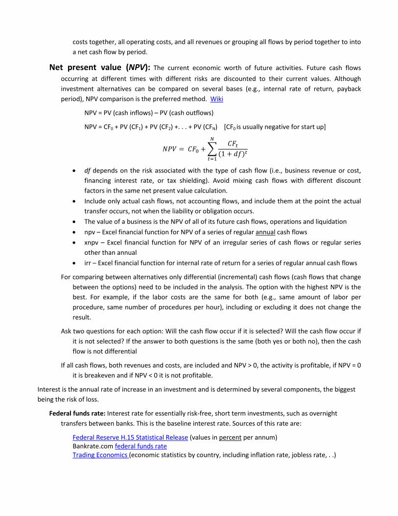
Net present value (NPV): The current economic worth of future activities. Future cash flows occurring at different times with different risks are discounted to their current values. Although investment alternatives can be compared on several bases (e.g., internal rate of return, payback period), NPV comparison is the preferred method. Wiki

NPV = PV (cash inflows) – PV (cash outflows)

NPV = CF0 + PV (CF1) + PV (CF2) +. . . + PV (CFN) [CF0 is usually negative for start up]

𝑁𝑃𝐹 = 𝐶𝐹0 + �𝐶𝐹𝑡

(1 + 𝑑𝑑)𝑡

𝑁

𝑡=1

• df depends on the risk associated with the type of cash flow (i.e., business revenue or cost, financing interest rate, or tax shielding). Avoid mixing cash flows with different discount factors in the same net present value calculation.

• Include only actual cash flows, not accounting flows, and include them at the point the actual transfer occurs, not when the liability or obligation occurs.

• The value of a business is the NPV of all of its future cash flows, operations and liquidation • npv – Excel financial function for NPV of a series of regular annual cash flows • xnpv – Excel financial function for NPV of an irregular series of cash flows or regular series

other than annual • irr – Excel financial function for internal rate of return for a series of regular annual cash flows

For comparing between alternatives only differential (incremental) cash flows (cash flows that change between the options) need to be included in the analysis. The option with the highest NPV is the best. For example, if the labor costs are the same for both (e.g., same amount of labor per procedure, same number of procedures per hour), including or excluding it does not change the result.

Ask two questions for each option: Will the cash flow occur if it is selected? Will the cash flow occur if it is not selected? If the answer to both questions is the same (both yes or both no), then the cash flow is not differential

If all cash flows, both revenues and costs, are included and NPV > 0, the activity is profitable, if NPV = 0 it is breakeven and if NPV < 0 it is not profitable.

Interest is the annual rate of increase in an investment and is determined by several components, the biggest being the risk of loss.

Federal funds rate: Interest rate for essentially risk-free, short term investments, such as overnight transfers between banks. This is the baseline interest rate. Sources of this rate are:

Federal Reserve H.15 Statistical Release (values in percent per annum) Bankrate.com federal funds rate Trading Economics (economic statistics by country, including inflation rate, jobless rate, . .)

LIBOR (London Interbank Offered Rate): Another interbank funds rate index often used for adjusting adjustable rate mortgages. Bankrate.com LIBOR

Inflation rate: The annual increase in costs of the same goods and services in an economy over an investment term, which differs depending on the particular goods and services. For families, this is the US Department of Labor BLS consumer price index, and for producers, the many BLS producer price indexes, all calculated by the Bureau of Labor Statistics. Because future inflation reduces the value of a dollar received for a dollar loaned, inflation forecasts based on economic indicators and federal monetary policy are incorporated into an inflation premium to adjust for this change in value.

𝐶𝐶𝐶𝐶𝐶𝐶𝐶𝐶𝐶𝐶𝑡𝐶𝐶𝐶𝐶𝐻𝐻𝐻𝑡𝐻𝐶𝐻𝐻𝐻𝐻

=𝐼𝐼𝑑𝐼𝐼𝐶𝐶𝐶𝐶𝐶𝐶𝑡𝐼𝐼𝑑𝐼𝐼𝐻𝐻𝐻𝑡𝐻𝐶𝐻𝐻𝐻𝐻

• Be careful not to span the index base date without adjusting for the re-indexing. • To adjust for the effects of inflation on expected prices of items such as supplies involved

in annual operating costs (e.g., fuel) use the recent rate of increase of the appropriate producer price index.

Thumb Rule of 72: The cost of an exactly equivalent item will approximately double or the value of a dollar will approximately halve in 72/(% inflation rate) years - wiki

Prime rate: Rate incorporating the real interest rate and an estimated inflation rate for low risk investments (e.g., loans to blue chip corporations), the reference interest rate (prime rate + X%) for many loans. Typically Federal funds rate + ~3% and reported by the Wall Street Journal Market Data Center - Bonds, Rates & Credit Markets. The prime rate components are not additive; rather per the Fisher equation:

(1 + 𝑑𝐼𝑑𝑑𝑑𝑑𝑑 𝑝𝑝𝑑𝑑𝐼 𝑝𝑑𝐶𝐼) = (1 + 𝑑𝐼𝑑𝑑𝑑𝑑𝑑 𝑝𝐼𝑑𝑑 𝑑𝐼𝐶𝐼𝑝𝐼𝐶𝐶)𝐼(1 + 𝑑𝐼𝑑𝑑𝑑𝑑𝑑 𝑑𝐼𝑑𝑑𝑑𝐶𝑑𝐶𝐼 𝑝𝑑𝐶𝐼)

𝑝𝑝𝑑𝑑𝐼 𝑝𝑑𝐶𝐼 = (1 + 𝑑𝐼𝑑𝑑𝑑𝑑𝑑 𝑝𝐼𝑑𝑑 𝑑𝐼𝐶𝐼𝑝𝐼𝐶𝐶)𝐼(1 + 𝑑𝐼𝑑𝑑𝑑𝑑𝑑 𝑑𝐼𝑑𝑑𝑑𝐶𝑑𝐶𝐼 𝑝𝑑𝐶𝐼) − 1

Real interest: Actual return on the investment, which includes the risk free rate of return for money plus a risk premium. The higher the probability of loss, the higher the risk premium. Higher risk investments (e.g., venture capital, lending to consumers with poor FICO scores, longer term) have higher interest rates than low risk investments (government bonds, lending to consumers with excellent FICO scores, shorter term).

Risk premium: The adjustment for expected loss risk associated with the investment. For loans, this is loan type, such as business loan, home mortgage, student loan, car loan, and consumer credit, with the loan term, with the amount of collateral that will be under lien, and with the borrower’s “Five C’s”. For business investments, this includes the leverage amount, the Beta of the industry, the difficulty of converting the asset to cash, and other things that fill corporate finance textbooks.

Federal Reserve Survey of Terms of Business Lending (business loans by term and risk)

For example of a no collateral loan, the current consumer credit risk premium for credit card holders with high FICO scores is ~9% (card APR – Prime Rate).

Federal Reserve Consumer Credit G.19 (interest rates by loan type and term)

An example of a loan with collateral is a home equity loan for which the risk premium for borrowers with high FICO scores is ~4.6% and ~5.1% for those with good scores.

An example of term effect is the risk premium difference between a 15 year fixed mortgage and 30 year, the 30 year being ~0.76% higher.

The long term risk premium of stocks over long term government bonds is 3 to 3.5% with a standard deviation of ~16%. For individual “safe” stocks, the risk premium is 4%, for the average (β = 1) stock, 8% and for relatively risky 16%. Diversifying the investment portfolio mitigates the risk of individual stocks. Note that the typical management fees for mutual funds effectively halve the long run return, which makes investment vehicles such as stock index funds with their considerably lower management fees more attractive.

MoneyChimp Stock CAGR (compound annual growth rate, annualized return)

“Five C’s of Credit” - lending and credit analysis for repayment ability: Capacity, capitalization, collateral, credit, character - capacity of business to service the loan (cash flow), proportion of total capital and personal equity (house, personal funds) contributed by the business owners (“skin in the game” – 20-25% typical, 50% for higher risk), sufficient collateral to guarantee the loan, credit history and current status (unpaid tax liabilities, current liens, civil judgments have to be paid before loan is granted), character (personal integrity, trustworthiness, responsibility and moral obligation), comparative performance (strength of financial statements, comparison with industry benchmarks, managerial experience of key personnel) and outside conditions (economic environment, technology trends, market trends, competition).

Continuing with an example, to have investment returns of $30,000 annually in perpetuity (without drawing on the principal) requires a current low-risk investment of ~$1,000,000. If your goal is to retire in 30 years and you expect to live at least 40 more years on a standard of living equivalent to that afforded by $30,000 currently, you have to convert the $1,000,000 to a future value using an estimated inflation rate over the 30 years. That is your investment target value at retirement. For the last 30 years, the US BLS CPI has ranged between -0.007 and 0.134 with a median of 0.030 and an average of 0.039. The calculator equation is (1+0.039)^30 or 3.15, meaning that your investment target is ~$3,150,000 at the time of your retirement for an annual return of $94,534 to live on, which are economically equivalent to $1M and $30K today. Check your answer by applying the rough thumb rule of 72 or 72/3.9 = 18.5 years for the amount needed to double.

𝑃𝐹 = 𝐴𝐻 Perpetuity, i = real interest rate

Nominal (stated) annual interest (r): the stated annual return that incorporates the projected inflation rate and the real interest rate without adjustment for compounding (if other than simple annual, which is rare)

(1 + 𝑝) = (1 + 𝑑𝐼𝑑𝑑𝑑𝑑𝑑 𝑑𝐼𝑑𝑑𝑑𝐶𝑑𝐶𝐼) ∗ (1 + 𝑑𝐼𝑑𝑑𝑑𝑑𝑑 𝑝𝐼𝑑𝑑 𝑑𝐼𝐶𝐼𝑝𝐼𝐶𝐶)

Nominal interest = inflation + “working “return + premium due to loss risk

Be sure to handle inflation consistently in your analyses, generally by using a nominal rate for cash flow value conversion, a real rate for real value conversion and an inflation rate for equivalent goods price conversion. Also note that the IRS does not allow adjustment of items such as salvage value and depreciation for inflation.

Firms lending you money have incentives to state the loan rate in the lowest form and to shift as many costs as they can out of the interest payments while firms investing your money have

incentives to state potential returns in the highest form and to disguise their fees. Small fee differences, say between 0.25% and 1%, result in major endpoint differences (SED pdf).

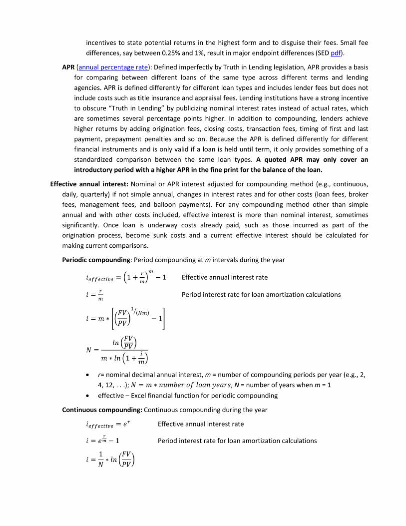
APR (annual percentage rate): Defined imperfectly by Truth in Lending legislation, APR provides a basis for comparing between different loans of the same type across different terms and lending agencies. APR is defined differently for different loan types and includes lender fees but does not include costs such as title insurance and appraisal fees. Lending institutions have a strong incentive to obscure “Truth in Lending” by publicizing nominal interest rates instead of actual rates, which are sometimes several percentage points higher. In addition to compounding, lenders achieve higher returns by adding origination fees, closing costs, transaction fees, timing of first and last payment, prepayment penalties and so on. Because the APR is defined differently for different financial instruments and is only valid if a loan is held until term, it only provides something of a standardized comparison between the same loan types. A quoted APR may only cover an introductory period with a higher APR in the fine print for the balance of the loan.

Effective annual interest: Nominal or APR interest adjusted for compounding method (e.g., continuous, daily, quarterly) if not simple annual, changes in interest rates and for other costs (loan fees, broker fees, management fees, and balloon payments). For any compounding method other than simple annual and with other costs included, effective interest is more than nominal interest, sometimes significantly. Once loan is underway costs already paid, such as those incurred as part of the origination process, become sunk costs and a current effective interest should be calculated for making current comparisons.

Periodic compounding: Period compounding at m intervals during the year

𝑑𝐶𝑑𝑑𝐶𝐻𝑡𝐻𝑒𝐶 = �1 + 𝐶𝑚�𝑚− 1 Effective annual interest rate

𝑑 = 𝐶𝑚

Period interest rate for loan amortization calculations

𝑑 = 𝑑 ∗ ��𝐹𝐹𝑃𝐹

�1

(𝑁𝑚)�− 1�

𝑁 =𝑑𝐼 �𝐹𝐹𝑃𝐹�

𝑑 ∗ 𝑑𝐼 �1 + 𝑑𝑑�

• r= nominal decimal annual interest, m = number of compounding periods per year (e.g., 2, 4, 12, . . .); 𝑁 = 𝑑 ∗ 𝐼𝑛𝑑𝑛𝐼𝑝 𝐶𝑑 𝑑𝐶𝑑𝐼 𝑦𝐼𝑑𝑝𝐶, N = number of years when m = 1

• effective – Excel financial function for periodic compounding

Continuous compounding: Continuous compounding during the year

𝑑𝐶𝑑𝑑𝐶𝐻𝑡𝐻𝑒𝐶 = 𝐼𝐶 Effective annual interest rate

𝑑 = 𝐼𝑟𝑚 − 1 Period interest rate for loan amortization calculations

𝑑 =1𝑁∗ 𝑑𝐼 �

𝐹𝐹𝑃𝐹

�

𝑁 =1𝑑∗ 𝑑𝐼 �

𝐹𝐹𝑃𝐹

�

• exp – Excel function for power to the base e

Amortization: The payment of principle and interest that pay down (“kill off”) a debt in regular installments (e.g., monthly, quarterly, annually) over a defined period (e.g., 60 months, 7 yrs, 15 yrs, 30 yrs) or the within business allocation of depreciation to annual charges for recovering the investment in an asset over its expected useful economic life. Canadian loan amortization is slightly different than US amortization. The loan amortization schedule is a table listing each payment (A), the amount that is interest and the amount applying to the loan principal balance. The two types of loan amortization plans are equal total payment or equal principal payment with declining total payment per installment.

Equal Payment Constant Series formulas:

𝑃𝐹 = 𝐴 ∗ �1−(1+𝐻)−𝑁

𝐻� [check: 𝑃𝐹 < 𝑁 ∗ 𝐴] Present Worth (P/A, i, N)

𝐴 = 𝑃𝐹 ∗ � 11−(1+𝐻)−𝑁

� = 𝑃𝐹 ∗ � 𝐻∗(1+𝐻)𝑁

(1+𝐻)𝑁−1� Capital Recovery (A/P, i, N)

𝐹𝐹 = 𝐴 ∗ �(1+𝐻)𝑁−1𝐻

� [check: 𝐹𝐹 > 𝑁 ∗ 𝐴] Compound Amount (F/A, i, N)

𝐴 = 𝐹𝐹 ∗ � 𝐻(1+𝐻)𝑁−1

� Sinking Fund (A/F, i, N)

• For analyzing loans, use the period loan interest rate (i) and for analyzing depreciation capital recovery, use the business discount rate (dr)

• The remaining balance of a loan is the PV of the N remaining payments, which is (total number of payments – number of payments already made)

Associated Excel financial functions (For on-line function help use “Help on this function” link in the Excel function box):

• Fv (i%, N, A) – series compound amount • Pv (i%, N, A) – series present worth • Nper (i%, A, - PV) – number of intervals required to pay off PV • Rate (N, A, - PV) – nominal interest rate being charged to pay off PV • pmt – periodic payment

o Sinking fund – pmt (i%, N, 0, FV) o Capital recovery – pmt (i%, N, P)

• Ipmt (i%, n, N, PV) – interest paid with the payment for interval n of N total intervals • ispmt – interest paid in a particular interval (more flexible than ipmt) • ppmt (i%, n, N, PV) – principal paid with the payment for interval n of N total intervals • cumipmt (i%, N, PV, nstart, nend, 0) – cumulative interest paid between the periods nstart and

nend • cumprinc – cumulative interest paid between two periods

(For additional help with spreadsheet financial functions, see finance or engineering texts based on Excel or on-line resources such as “Microsoft Excel as a Financial Calculator”)

For equal payment loans the early payments are mostly interest and very little principal. Most principal reduction occurs toward the end of the loan. The lower the interest rate and the shorter the term, the closer the balance decline is to a straight line. For a 30 year loan @ 8% at the 1/2 of term ~80% of principal remains and 1/2 of principal remains at ~23/30 year. Compare loan options on the basis of NPV’s that include all costs and tax effects (Fortin et al. 2007). Consider refinancing carefully because restarting the clock means additional interest expense and delayed reduction of the principal unless the new loan is for a shorter term. Unless you are refinancing to reduce critical liquidity (cash flow) problems, make your refinancing decision by comparing the current NPV’s of the amortization schedules between your current loan at this time and proposed loans, not the reduction in monthly payments. The origination fees and interest already paid on your current loan are sunk costs. What counts is comparing the current NPV of your present loan, which is the PV of the remaining payments if you continued the loan to term, with the NPV of the new loan plus any early payment penalties for your existing loan.

Negative amortization: The payment does not cover the interest for the period and the balance due is added to the loan principle, which occurs with some types of graduated rate, adjustable rate, and reverse mortgages.

Discount rate: Your business “cost of capital,” which is the annual discount rate you use for converting a future business cash flow, revenue or expense, to a present value for NPV analysis that is appropriate for the risk level of the “project.”

Determining the appropriate MARR (minimum acceptable rate of return) or “hurdle rate” is critical for making sound investment decisions. The minimum is the effective interest rate on borrowed money (if simply not taking out the loan is the alternative) for the investment plus a risk premium (the lending agency is less likely to lose their money than you are, especially if they have collateral) or, if you have the money in hand, the rate of return on your next most attractive investment option of similar risk. If the debt is on a credit card, the discount rate should be the effective card interest rate plus a risk premium (again, the card provider is less likely to lose money than you). If in hand money could be invested through a financial institution, the opportunity cost is the riskless rate plus the risk premium for your preferred investment. If that was a stock index fund, the stock market historical long-run return has averaged 6% over inflation (but ranging from -2% to 13% and as low as 2% for two recent decades - MoneyChimp Stock CAGR) so a projected long-term stock market return might be 10% (historical stock market return + historical inflation rate). In that case, any investment in the business should have a rate of return of at least 10% plus a risk premium so using an effective interest rate of 10% for present value calculations is reasonable if the risks of loss are equivalent. On the other hand, if the money is under your mattress where it is losing value at the inflation rate (or gaining at the deflation rate) the rate could be only the risk premium.

Minimum Acceptable (attractive) Rate of Return (MARR, hurdle rate) = Cost of capital + risk premium- wiki

Examples of stock index fund and exchange traded (ETFs) funds (no endorsement intended or implied) that are potential alternative investments:

• Vanguard 500 Index

• Schwab S&P 500 Index Fund • Charles Schwab Exchange Traded Funds

Equal marginal principle: Within the business, invest scarce resources (e.g., time, money) in those things that have the highest marginal return (marginal revenue – marginal cost) to the point that their marginal return drops below that of the next best alternative, that MR = MC or for all cash flows NPV < 0.

Equipment costs are classified as either ownership or operating costs. Although little information is available for veterinary medical equipment, considerable agricultural equipment cost evaluation information is on-line. If these are based on accrual accounting, the analytical processes are applicable to veterinary equipment but the tax depreciation schedules and rates are likely different.

A large corporate practice using a 20% rate of return has a thumb rule that new equipment must generate annual new gross income at least equal to 40% of its purchase cost.

Note that this effect occurs with salaries. Dr. M.L. Heinke (2010) estimates that a veterinarian with a salary of $80,000 working 40 hrs/wk, 50 weeks per year or 2,000 hours has to generate $400,000 of services to cover salary, overhead, support staff and profit in a typical small animal practice. If 50% of the time is billable work, that veterinarian has to generate $400 of practice gross income per productive hour (DVM Magazine, Feb 01, 2010).

For agricultural examples, see Kastens T (1997) “Farm Machinery Operation Cost Calculations” mf-2244, Kansas State University, Williams and Kastens (1998). Lease, Custom Hire, Rent or Purchase Farm Machinery: Evaluating the Options (proceedings pdf), or Iowa State’s “Estimating Farm Machinery Costs”A3-29.

Annual ownership costs: The costs, mostly fixed, that occur due to owning the item and further classified under the acronym “DIRTI 5” – depreciation, interest, repairs, storage, taxes, and insurance. Typical equipment ownership costs are initially high due to the initial rapid value loss in the transition from new to used, decline to a minimum and then rise as repair costs increase.

Depreciation: The decline in asset value due to age. The fixed component is the loss of value due to the passage of time, such as technical obsolescence or general deterioration. The variable cost component is the loss of value due to the amount of use. Current market value is adjusted upward from typical values for equipment with less use and in better condition and downward for equipment with more use and in poorer condition. Depreciation is usually the largest annual ownership cost. Wiki

Cost basis (CB): Invoice price, sales tax, shipping cost, installation costs including facility modifications and one-time permit, testing, and inspection fees.

Salvage value (SV): The expected market value of an equipment item when it is sold. If the item is expected to have no market value but to have removal and disposal costs, the salvage value is negative.

Economic depreciation: The decline in current salvage (market) value, which is rapid at first (driving a new car off the lot) and then slows. Methods such as the “Sum of the Years Digits” account for the more rapid decline that occurs in early life. “Straight line” is the simplest but the current straight line depreciated value may not represent the current salvage value as well

as other methods. A rough rule of thumb is that farm equipment depreciates approximately 10% annually.

syd – Excel function for “sum of the years digit” depreciation

Tax depreciation: The depreciation method selected from the tax code in force at the time of equipment purchase to minimize taxes based on the equipment type, purchase and use conditions. Rather than being expensed in the year of purchase, this ownership cost is expensed as a deductible business expense across multiple years. Modified Accelerated Cost Recovery System (MACRS) described in IRS Publication 946 (2009), “How to Depreciate Property” details the approved methods and years for depreciating most business and investment property for tax purposes. IRS Publication 225, “Farmer’s Tax Guide,” contains the equivalent information for farming businesses. Tax (book) value may be different than current salvage value and generally overestimates ownership expense early and underestimates it later in the equipment’s useful life. Tax adjustments are required if the salvage or terminal value (sale price) differs from the equipment’s book (tax) value at the end of it’s useful life in the business.

Depreciation itself is not an actual cash flow but rather reduces cash outflow by decreasing (shielding) taxes.

Depreciation Tax Shield = (annual tax depreciation) x (marginal tax rate)

Note that the IRS can change the tax code at any time and the changes can be retroactive. Hence, if it doesn’t make sense economically, be careful of doing it for tax purposes. Even for tax purposes, it still costs you (depreciation) x (1 – tax rate).

Depreciable property: To be depreciable, the property must be used in business or held to produce income (e.g., rental property), it must have a definable service life that is longer than a year, and it must wear out, get used up, become obsolete or decay. Intangible property such as customer lists, franchises, patents, designs, copyrights and computer software are depreciable. Land is not but buildings are.

Recovery period: Service life of equipment for tax purposes. Examples for illustration only (check the current regulations!) from IRS Publication 946 are 5 years for automobiles, breeding cattle, computers, pickups, and high technology medical equipment, 7 years for agricultural equipment, office fixtures and any equipment not otherwise classified, 10 years for sole purpose agricultural structures.

Value estimation: If a current value isn’t known but historical value of an identical item (same model, similar usage) is, the historical value can be adjusted using the historical and current values of the appropriate index (PPI, CPI).

𝐶𝐶𝐶𝐶𝐶𝐶𝐶𝐶𝐶𝐶𝑡𝐶𝐶𝐶𝐶𝐻𝐻𝐻𝑡𝐻𝐶𝐻𝐻𝐻𝐻

=𝐼𝐼𝑑𝐼𝐼𝐶𝐶𝐶𝐶𝐶𝐶𝑡𝐼𝐼𝑑𝐼𝐼𝐻𝐻𝐻𝑡𝐻𝐶𝐻𝐻𝐻𝐻

Insurance: Annual property insurance cost. If not known, for farm equipment this is ~ 0.25% of purchase cost. Insure against potential catastrophic loss but don’t insure against potential losses that you could afford.

Repairs: Annual cost of repairs and normal upkeep. Historical repair records for similar equipment in similar use provide the best estimates of expected repair costs. For major repairs (e.g. broken ultrasound probe, transmission replacement), the annual cost is the estimated probability of the repair being needed during the period times the cost of the repair.

ASABE Standard EP496.3 “Agricultural Machinery Management” section 6.3.1 contains a repair cost formula for tractors and D497.7 “Agricultural Machinery Management Data” for other equipment.

Storage: Annual housing costs if unique and attributable to this equipment, such as a heated garage for a practice vehicle. If not known, for farm equipment this is ~ 0.75% of purchase cost.

Taxes: Annual government fees, such as property taxes, licensing fees, and waste permits (if applicable) that can be apportioned to this equipment. If not known, for farm equipment this is ~ 1% of purchase cost.

Interest: The annual opportunity cost of the funds invested in the equipment.

Annual Capital Recovery (ACR): The annual ownership cost due to the capital investment.

𝐴𝐶𝐴 = (𝐶𝐶 − 𝑆𝐹) ∗ �𝑑𝑝

1 − (1 + 𝑑𝑝)−𝑁� + (𝑆𝐹 ∗ 𝑑𝑝)

𝐴𝐶𝐴 = (𝐶𝐶 − 𝑆𝐹) ∗ �𝑑𝑝

(1 + 𝑑𝑝)𝑁 − 1� + (𝐶𝐶 ∗ 𝑑𝑝)

Be careful of double counting by including ACR in NPV analyses. This is not a cash flow. The purpose of ACR is to provide a quick estimate of the annual capital costs of ownership

Operating costs: Costs incurred when the equipment operates. These include operator labor, energy (fuel, electricity) and supplies consumed (e.g. disposable sheaths, disinfectant solutions).

Total Annual Cost = Annual Ownership Cost + Annual Operating Cost

Be careful of double counting by including total annual cost in NPV analyses.

Net Present Value Analysis Steps:

1. Identify and forecast the relevant incremental cash flows and opportunity costs for each alternative

For comparing competing alternatives only differential (incremental) cash flows (cash flows that change between the options) for each period need to be included in the analysis. The option with the highest NPV is the best. For example, if revenue and the labor costs are the same for both (e.g., same amount of labor per procedure, same number of procedures per hour), including or excluding these does not change the conclusion.

Considering the business as a box that cash flows into and out of, exclusive of financing cash flows. For each option, the incremental cash flows are the changes in those cash inflows and cash outflows due to the option.

For each option, ask two questions for each period of its economic lifetime. Will the cash flow into or out of the business occur if it is selected? Will the same cash flow occur if it is not selected? If the answer to both questions is the same (both yes or both no), then the cash flow is not differential

If slack (unused) salaried time is employed, there is no opportunity cost for that resource. If salaried time is not slack but is shifted from doing something else, an opportunity cost is likely involved.

2. Adjust for inflation and income tax effects

Adjust the costs of inputs, such as gasoline, disposables, and wages, that are components of incremental costs for the effects of inflation over each option’s economic life

If service charges are incremental, adjust them for inflation over the economic life of each option

3. Draw the cash flow diagrams for each option, using separate diagram for each discount rate and type of cash flow if that makes your analysis clearer

4. Calculate discounted cash flows by converting the nominal after-tax cash flow values to net present values using the appropriate discount rates and calculate the NPV of the alternative.

NPV = CFStart + PV (operating CF1) + PV (operating CF2) +. . . + PV (CFTermination)

• CFStart is usually negative for startup (equipment purchase, training, working capital increase for inventory) and is usually positive for CFTermination (salvage, working capital decrease from dispersing inventory)

𝑁𝑃𝐹 = 𝐶𝐹0 +�𝐶𝑛𝐶𝑑𝐼𝐼𝐶𝐶 𝐶𝐹𝑡

(1 + 𝑑𝑝)𝑡

𝑁

𝑡=1

+ �𝐹𝑑𝐼𝑑𝐼𝑑𝑑𝐼𝐹 𝐶ℎ𝑑𝐼𝑑𝑑 𝐶𝐹𝑡

(1 + 𝑑)𝑡

𝑁

𝑡=1

+�𝐷𝐼𝑝𝑝𝐼𝑑𝑑𝑑𝐶𝑑𝐶𝐼 𝐶ℎ𝑑𝐼𝑑𝑑 𝐶𝐹𝑡

(1 + 𝑝)𝑡

𝑁

𝑡=1

+ 𝐶𝐹𝑁

NPV = PV (after tax net profits) + PV (tax shielding of debt undertaken for option) + PV (tax shielding of depreciation)

• Tax shielding of debt = the tax deductions due to mortgage interest deductions, investment credits and so on.

Separate financing decisions from capital investment decisions so that you make capital investment decisions on their NPV merits and financing decisions on theirs. Disentangle combined offers, such as payment plans or leasing vs. buying decisions, so that the purchase decision is separate from the financing decision.

• For calculating PV of revenues and costs, use your business discount rate dr • For calculating PV of financing including the PV of tax shielding of interest or other tax

deductions associated with borrowing, use the effective annual loan rate i • For calculating PV of depreciation, use a low risk rate (the IRS is unlikely to cancel depreciation,

go bankrupt or insist on a risk premium) 5. Compare the alternatives on the basis of their NPV’s.

If all cash flows, both revenues and costs, are included and NPV > 0, an activity is profitable, if NPV = 0 it is breakeven and if NPV < 0 it is not profitable.

If a current service has an NPV < 0 when all cash flows are included then unless it has to be done even if unprofitable investment should be reduced or sold until the NPV = 0 (true breakeven), and the resulting funds invested elsewhere. This is particularly true if the risk of loss from an alternative is lower. If the service with an NPV < 0 is required to maintain other profitable activities (e.g., client expects night emergency service in exchange for doing his herd work), then the loss should be

charged to those other activities that require this one to continue. If the service involves a significant equipment investment, carefully consider different exit strategies.

When choosing between alternative services, expand the one with the higher NPV until NPV (best) = NPV (second best). At some point, your market will not support further expansion (e.g., you are already palpating all the cows in the area) or the cost of delivering that service rises to the point that delivering other services is equally profitable (e.g., the next closest client for this service is too far away).

Alternatives having unequal lifetimes are a special case. An example is a replacement decision involving equipment with different expected lives (e.g., Do I replace the transmission in the old pickup and anticipate that it will last three more years or do I replace it with a new one that I expect will last 9 years?). One strategy is to use a number of years that is a common multiple of the lifetimes of both alternatives (repaired old pickup lasts 3 more years, new pickup lasts 9 years, compare the NPV of 3 cycles of the old pickup vs. the NPV of one cycle of purchasing new pickup). Another strategy is to convert both NPV’s to the equivalent annual cost (EAC) or annuity equivalent for each alternative.

𝐸𝐴𝐶 = 𝑁𝑃𝐹 ∗ �1

1 − (1 + 𝑑𝑝)−𝑁� = 𝑁𝑃𝐹 ∗ �

𝑑𝑝 ∗ (1 + 𝑑𝑝)𝑁

(1 + 𝑑𝑝)𝑁 − 1�

• N = lifetime left for this alternative 6. Perform sensitivity analyses for the important variables and “What if?” scenario analysis for the best

and worst case scenarios

Determine the relative importance of costs by group (e.g., depreciation, operating cost, interest cost) by dividing the NPV of each group by the total NPV.

To evaluate the influence of uncertainty on decisions, perform a sensitivity analysis by evaluating expected case, best case and worst case scenarios for each input variable.

What are the important variables to monitor (e.g., number of procedures, variable costs) and what levels trigger concern and reevaluation? What are the consequences if your estimate is off by ±10%? Graph NPV against cost of capital discount rate.

Spreadsheet spider and tornado graphs show the effects of input parameter variations graphically.

For an agricultural examples of NPV analyses, see Capital Investment Analysis and Project Assessment, Purdue Extension EC-731, or Capital Budgeting for a New Dairy Facility, CV Thomas, MA DeLorenzo and DR Bray, University of Florida CIR1110 (pdf) and the associated spreadsheet CapitalBudget.xls.

Real options: wiki

Real options is a capital budgeting method that values future flexibility. The basic idea is that a project is not static once underway but will be modified as new information becomes available.

References and Resources:

• Ackerman L (2002). Business Basics for Veterinarians - Amazon • Ackerman L (2003). Management Basics for Veterinarians - Amazon • Ackerman L (2006). Blackwell’s Five-minute Veterinary Practice Consult - Amazon • Anon. (rev 2015). Estimating farm machinery costs. Iowa State University File A3-29, PM 710 - pdf • Boehlje M, C Ehmke (2005). Capital investment analysis and project assessment (Purdue EC-731) - pdf • Bogle JC (2005). The relentless rules of humble arithmetic. Financial Analysts J 61(6):22-35) • Danielson MG, JA Scott (2006). The capital budgeting decisions of small businesses - pdf • Fortin R, S Michelson, SD Smith, W Weaver (2007). Mortgage refinancing: the interaction of break even period,

taxes, NPV, and IRR. Financial Services Review, 16(3):197-209 . • Kastens T (1997) “Farm Machinery Operation Cost Calculations” mf-2244 • Kurtz M (1995). Calculations for Engineering Economic Analysis. McGraw-Hill, Inc. • Heinke, ML (2010). Fee Setting: A look at margins, DVM Magazine Feb 01, 2010 • Higgins, RC.(2008). Analysis for Financial Management, 10th ed. - Amazon • Newman DG, TG Eschenbach, JP Lavelle (2011). Engineering Economic Analysis, 11th ed. Oxford Press Amazon • Olson K (2011). Economics of Farm Management in a Global Setting - Amazon • Park, CS (2012). Fundamentals of Engineering Economics, 3rd ed. Pearson Education Inc. – book website Amazon • Powell SG, KR Baker, B Lawson (2008). A critical review of the literature on spreadsheet errors. Decision Support

Systems 46:128-138. pdf Spreadsheet Engineering, Tuck at Dartmouth • Sepulveda J, WE Souder, BS Gottfried (1984). Schaum’s Outline of Engineering Economics, McGraw-Hill - Amazon • Sherrick BJ, PN Ellinger, DA Lins (2000). Time value of money and investment analysis: Explanations and

spreadsheet application applications for agricultural and agribusiness firms. Part I – pdf; Part II - pdf • Shim JK, JG Siegel (2008). Financial Management, 3rd ed. (Barron's Business Library) - Amazon • Social Security Advisory Board (2001). Estimating the real rate of return on stocks over the long term. - pdf • Sullivan WG, EM Wicks, CP Koelling (2014). Engineering Economy, 16th ed. Amazon • Williams J, T Kastens (1998). Lease, custom hire, rent or purchase farm machinery: Evaluating the options.

Department of Agricultural Economics Risk and Profit Conference, Kansas State University, August 20-21, 1998 (proceedings pdf)

Additional Information and Tools: (alphabetical, no endorsement implied nor verification performed)

The Internet abounds with resources such as class handouts, worked problems, on-line calculators and even on-line books. Below are some that I’ve happened across but there are many more, some of which may be much better than these.

• Accounting Details Income Tax and Capital Budgeting Decisions

• AVMA Member Benefits - Bank of America Practice Solutions, Inc Resources for Health Care Practice Financing Principles of Finance with Excel (2005).– pdf

• Bogleheads.org – Investing advice inspired by Jack Bogle, founder of The Vanguard Group • CalculatorsPlus.com – Finance & Loan Calculators • Choose to Save Calculators (Employee Benefit Research Institute, American Savings Education Council) • Damodaran, A. Prof of Finance, Stern School of Business– spreadsheets, class notes • Drake, PP, Prof of Finance, James Madison U -

Principles of financial management Learning Resources in Finance

• Evans, MH – Financial Management Training Center - spreadsheets • FAST: Farm Analysis Solution Tools, U Illinois • FinAid: The SmartStudent Guide to Financial Aid - Calculators • Financial Power Tools Calculators • Gelinas, M. The lost art of Interest calculation – white paper. • Guttentag, JM, Wharton professor emeritus - The Mortgage Professor’s Website • Keys, J Instructor, Florida Intl U (Chang, CH) • Mahar, Jim, Prof of Finance, St. Bonaventure U, FinanceProfessor.com • Math4Finance.com - Financial math formulas and financial equations • Mayes, TR, Prof of Finance, Metropolitan State College of Denver – Excel blog

Financial Analysis with Microsoft Excel - Amazon TVM Calcs.com: Time value math

• How to think about time value of money problems – html • Microsoft Excel as a Financial Calculator - html

• Moneychimp – Compound Annual Growth Rate – Stock Market • Mortgage-X - calculators • Rumelt, RP, Professor of Business Strategy, UCLA – instructional notes (Numbers 101) • Scordo, JP – Latest journal articles and working papers in finance • Shiller, Robert, Yale Nobel Laureate economist - wiki – S&P/Case-Shiller Home Price Indices • Applied Finance – Self-paced Overviews of Fundamentals of Applied Finance, U Arizona • VeterinaryLoans.com • Wachowicz, JM, Prof of Finance, U Tennessee – Web World: websites for discerning finance students • Womack, KL, Prof of Finance, Rotman School of Management, U Toronto (deceased)

Financial Math on Spreadsheet and Calculator, 4.0, 2002 - ssn papers pdf The top ten books on his Decision Making Course Bookshelf - Amazon

• Moneyball: The Art of Winning an Unfair Game • Influence: Science and Practice • Nudge: Improving Decisions About Health, Wealth, and Happiness • Switch: How to Change Things When Change Is Hard • Complications: A Surgeon's Notes on an Imperfect Science • The Seven Sins of Memory: How the Mind Forgets and Remembers • Mistakes Were Made (But Not by Me): Why We Justify Foolish Beliefs, Bad Decisions, and Hurtful Acts • Into Thin Air: A Personal Account of the Mt. Everest Disaster • How Doctors Think • Stumbling on Happiness