Visualizing Dataflow Graphs ofDeep Learning Models in TensorFlow

Kanit Wongsuphasawat, Daniel Smilkov, James Wexler, Jimbo Wilson,Dandelion Mane, Doug Fritz, Dilip Krishnan, Fernanda B. Viegas, and Martin Wattenberg

(a) (b)

Main Graph Auxiliary Nodes

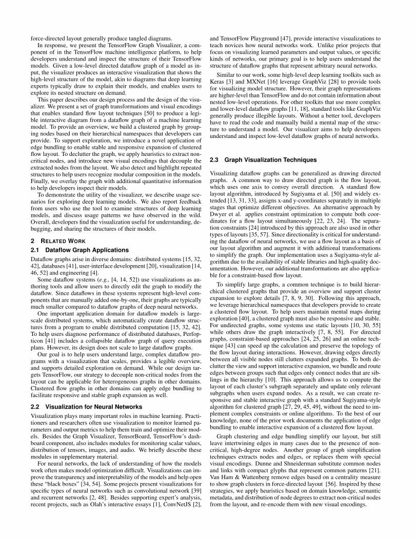
Fig. 1. The TensorFlow Graph Visualizer shows a convolutional network for classifying images (tf cifar) . (a) An overview displaysa dataflow between groups of operations, with auxiliary nodes extracted to the side. (b) Expanding a group shows its nested structure.

Abstract—We present a design study of the TensorFlow Graph Visualizer, part of the TensorFlow machine intelligence platform. Thistool helps users understand complex machine learning architectures by visualizing their underlying dataflow graphs. The tool worksby applying a series of graph transformations that enable standard layout techniques to produce a legible interactive diagram. Todeclutter the graph, we decouple non-critical nodes from the layout. To provide an overview, we build a clustered graph using thehierarchical structure annotated in the source code. To support exploration of nested structure on demand, we perform edge bundlingto enable stable and responsive cluster expansion. Finally, we detect and highlight repeated structures to emphasize a model’smodular composition. To demonstrate the utility of the visualizer, we describe example usage scenarios and report user feedback.Overall, users find the visualizer useful for understanding, debugging, and sharing the structures of their models.

Index Terms—Neural Network, Graph Visualization, Dataflow Graph, Clustered Graph.

1 INTRODUCTION

Recent years have seen a series of breakthroughs in machine learning,with a technique known as deep learning bringing dramatic results onstandard benchmarks [37]. A hallmark of deep learning methods is

• Kanit Wongsuphasawat is with Paul G. Allen School of Computer Science& Engineering, University of Washington. E-mail: kanitw@uw.edu.

• Daniel Smilkov, James Wexler, Jimbo Wilson, Dandelion Mane, Doug Fritz,Dilip Krishnan, Fernanda B. Viegas, and Martin Wattenberg are withGoogle Research. E-mail: {smilkov, jwexler, jimbo, dougfritz, dilipkay,viegas, wattenberg}@google.com

Manuscript received xx xxx. 201x; accepted xx xxx. 201x. Date ofPublication xx xxx. 201x; date of current version xx xxx. 201x.For information on obtaining reprints of this article, please sende-mail to: reprints@ieee.org.Digital Object Identifier: xx.xxxx/TVCG.201x.xxxxxxx/

their multi-layered networks of calculations. The complexity of thesenetworks, which often include dozens of layers and millions of param-eters, can lead to difficulties in implementation. Modern deep learningplatforms including TensorFlow [6], Theano [11], and Torch [18] pro-vide high-level APIs to lower these difficulties. With these APIs, de-velopers can write an abstract program to generate a low-level dataflowgraph that supports a variety of learning algorithms, distributed com-putation, and different kinds of devices.

These APIs and their dataflow models simplify the creation of neu-ral networks for deep learning. Yet developers still have to read codeand manually build a mental map of a model to understand its com-plicated structure. A visualization of the model can help developersinspect its structure directly. However, these dataflow graphs typicallycontain thousands of heterogeneous, low-level operations; some ofwhich are high-degree nodes that connect to many parts of the graphs.As a result, standard layout techniques such as flow layout [49] and

force-directed layout generally produce tangled diagrams.In response, we present the TensorFlow Graph Visualizer, a com-

ponent of in the TensorFlow machine intelligence platform, to helpdevelopers understand and inspect the structure of their TensorFlowmodels. Given a low-level directed dataflow graph of a model as in-put, the visualizer produces an interactive visualization that shows thehigh-level structure of the model, akin to diagrams that deep learningexperts typically draw to explain their models, and enables users toexplore its nested structure on demand.

This paper describes our design process and the design of the visu-alizer. We present a set of graph transformations and visual encodingsthat enables standard flow layout techniques [50] to produce a legi-ble interactive diagram from a dataflow graph of a machine learningmodel. To provide an overview, we build a clustered graph by group-ing nodes based on their hierarchical namespaces that developers canprovide. To support exploration, we introduce a novel application ofedge bundling to enable stable and responsive expansion of clusteredflow layout. To declutter the graph, we apply heuristics to extract non-critical nodes, and introduce new visual encodings that decouple theextracted nodes from the layout. We also detect and highlight repeatedstructures to help users recognize modular composition in the models.Finally, we overlay the graph with additional quantitative informationto help developers inspect their models.

To demonstrate the utility of the visualizer, we describe usage sce-narios for exploring deep learning models. We also report feedbackfrom users who use the tool to examine structures of deep learningmodels, and discuss usage patterns we have observed in the wild.Overall, developers find the visualization useful for understanding, de-bugging, and sharing the structures of their models.

2 RELATED WORK

2.1 Dataflow Graph ApplicationsDataflow graphs arise in diverse domains: distributed systems [15, 32,42], databases [41], user-interface development [20], visualization [14,46, 52] and engineering [4].

Some dataflow systems (e.g., [4, 14, 52]) use visualizations as au-thoring tools and allow users to directly edit the graph to modify thedataflow. Since dataflows in these systems represent high-level com-ponents that are manually added one-by-one, their graphs are typicallymuch smaller compared to dataflow graphs of deep neural networks.

One important application domain for dataflow models is large-scale distributed systems, which automatically create dataflow struc-tures from a program to enable distributed computation [15, 32, 42].To help users diagnose performance of distributed databases, Perfop-ticon [41] includes a collapsible dataflow graph of query executionplans. However, its design does not scale to large dataflow graphs.

Our goal is to help users understand large, complex dataflow pro-grams with a visualization that scales, provides a legible overview,and supports detailed exploration on demand. While our design tar-gets TensorFlow, our strategy to decouple non-critical nodes from thelayout can be applicable for heterogeneous graphs in other domains.Clustered flow graphs in other domains can apply edge bundling tofacilitate responsive and stable graph expansion as well.

2.2 Visualization for Neural NetworksVisualization plays many important roles in machine learning. Practi-tioners and researchers often use visualization to monitor learned pa-rameters and output metrics to help them train and optimize their mod-els. Besides the Graph Visualizer, TensorBoard, TensorFlow’s dash-board component, also includes modules for monitoring scalar values,distribution of tensors, images, and audio. We briefly describe thesemodules in supplementary material.

For neural networks, the lack of understanding of how the modelswork often makes model optimization difficult. Visualizations can im-prove the transparency and interpretability of the models and help openthese “black boxes” [34, 54]. Some projects present visualizations forspecific types of neural networks such as convolutional network [39]and recurrent networks [2, 48]. Besides supporting expert’s analysis,recent projects, such as Olah’s interactive essays [1], ConvNetJS [2],

and TensorFlow Playground [47], provide interactive visualizations toteach novices how neural networks work. Unlike prior projects thatfocus on visualizing learned parameters and output values, or specifickinds of networks, our primary goal is to help users understand thestructure of dataflow graphs that represent arbitrary neural networks.

Similar to our work, some high-level deep learning toolkits such asKeras [3] and MXNet [16] leverage GraphViz [28] to provide toolsfor visualizing model structure. However, their graph representationsare higher-level than TensorFlow and do not contain information aboutnested low-level operations. For other toolkits that use more complexand lower-level dataflow graphs [11, 18], standard tools like GraphVizgenerally produce illegible layouts. Without a better tool, developershave to read the code and manually build a mental map of the struc-ture to understand a model. Our visualizer aims to help developersunderstand and inspect low-level dataflow graphs of neural networks.

2.3 Graph Visualization Techniques

Visualizing dataflow graphs can be generalized as drawing directedgraphs. A common way to draw directed graph is the flow layout,which uses one axis to convey overall direction. A standard flowlayout algorithm, introduced by Sugiyama et al. [50] and widely ex-tended [13, 31, 33], assigns x-and y-coordinates separately in multiplestages that optimize different objectives. An alternative approach byDwyer et al. applies constraint optimization to compute both coor-dinates for a flow layout simultaneously [22, 23, 24]. The separa-tion constraints [24] introduced by this approach are also used in othertypes of layouts [35, 57]. Since directionality is critical for understand-ing the dataflow of neural networks, we use a flow layout as a basis ofour layout algorithm and augment it with additional transformationsto simplify the graph. Our implementation uses a Sugiyama-style al-gorithm due to the availability of stable libraries and high-quality doc-umentation. However, our additional transformations are also applica-ble for a constraint-based flow layout.

To simplify large graphs, a common technique is to build hierar-chical clustered graphs that provide an overview and support clusterexpansion to explore details [7, 8, 9, 30]. Following this approach,we leverage hierarchical namespaces that developers provide to createa clustered flow layout. To help users maintain mental maps duringexploration [40], a clustered graph must also be responsive and stable.For undirected graphs, some systems use static layouts [10, 30, 55]while others draw the graph interactively [7, 8, 55]. For directedgraphs, constraint-based approaches [24, 25, 26] and an online tech-nique [43] can speed up the calculation and preserve the topology ofthe flow layout during interactions. However, drawing edges directlybetween all visible nodes still clutters expanded graphs. To both de-clutter the view and support interactive expansion, we bundle and routeedges between groups such that edges only connect nodes that are sib-lings in the hierarchy [10]. This approach allows us to compute thelayout of each cluster’s subgraph separately and update only relevantsubgraphs when users expand nodes. As a result, we can create re-sponsive and stable interactive graph with a standard Sugiyama-stylealgorithm for clustered graph [27, 29, 45, 49], without the need to im-plement complex constraints or online algorithms. To the best of ourknowledge, none of the prior work documents the application of edgebundling to enable interactive expansion of a clustered flow layout.

Graph clustering and edge bundling simplify our layout, but stillleave intertwining edges in many cases due to the presence of non-critical, high-degree nodes. Another group of graph simplificationtechniques extracts nodes and edges, or replaces them with specialvisual encodings. Dunne and Shneiderman substitute common nodesand links with compact glyphs that represent common patterns [21].Van Ham & Wattenberg remove edges based on a centrality measureto show graph clusters in force-directed layout [56]. Inspired by thesestrategies, we apply heuristics based on domain knowledge, semanticmetadata, and distribution of node degrees to extract non-critical nodesfrom the layout, and re-encode them with new visual encodings.

3 BACKGROUND: TENSORFLOW

TensorFlow [6] is Google’s system for the implementation and deploy-ment of large-scale machine learning models. Although deep learningis a central application, TensorFlow also supports a broad range ofmodels including other types of learning algorithms.

The Structure of a TensorFlow Model

A TensorFlow model is a dataflow graph that represents a computation.Nodes in the graph represent various operations. These include mathe-matical functions such as addition and matrix multiplication; constant,sequence, and random operations for initializing tensor values; sum-mary operations for producing log events for debugging; and variableoperations for storing model parameters.

Edges in TensorFlow graphs serve three different purposes. Datadependency edges represent tensors, or multidimensional arrays, thatare input and output data of the operations. Reference edges, or out-puts of variable operations, represent pointers to the variable ratherthan its value, allowing dependent operations (e.g., Assign) to mutatethe referenced variable. Finally, control dependency edges do not rep-resent any data but indicate that their source operations must executebefore their tail operations can start.

Building a TensorFlow Model

The TensorFlow API provides high-level methods for produc-ing low-level operations in the dataflow graph. Some, such astf.train.GradientDescentOptimizer, generate dozens of low-level operations. Thus a small amount of code, such as the definitionof the tf mnist simple model in Figure 4 (see supplementary mate-rial), can produce about a hundred operations in the graph. Real-worldnetworks can be even more complex. For instance, an implementationof the well-known Inception network [51] has over 36,000 nodes.

Operation Names

For clarity, operations in TensorFlow graphs have unique names,which are partly generated by the API and partly specified by users.Slashes in operation names define hierarchies akin to Unix paths(like/this/example). By default, the API uses operation typesas names and appends integer suffixes to make names unique (e.g.,“Add 1”). To provide a meaningful structure, users can group oper-ations with a namespace prefix (e.g., “weights/”). Complex meth-ods such as tf.train.GradientDescentOptimizer also automat-ically group their underlying operations into subnamespaces (e.g.,“gradients” and “GradientDescent”). As discussed later in §5.2,we apply these namespaces to build a clustered graph.

4 MOTIVATION & DESIGN PROCESS

The motivation for the TensorFlow Graph Visualizer came from ourconversations with deep learning experts, including one of the authors.When experts discuss their models, they frequently use diagrams (e.g.,Figure 2) to depict high-level structure. When working with a newmodel, they often read the code and draw a diagram to help them builda mental map of the model’s architecture. Since diagrams are criticalfor their work, machine learning experts desire a tool that can auto-matically visualize the model structures.

Motivated by an apparent need for a visualization tool, we workedwith potential users to understand the key tasks for such a visualiza-tion. We also examined the model data that a visualization would haveto portray. The purpose of these investigations was to match user needswith what would be possible given real-world data.

Fig. 2. Whiteboard drawing by a computer vision expert: a convolu-tional network for image classification.

4.1 Task AnalysisOur overarching design goal is to help developers understand and com-municate the structures of TensorFlow models, which can be usefulin many scenarios. Based on conversations with potential users, weidentified a set of key scenarios for a model visualization. Beginnersoften learn how to use TensorFlow based on example networks in thetutorials. Even experts usually build new models based on existingnetworks. Therefore, they can use the visualization to help them un-derstand existing models. When modifying the code that generatesmodels, developers can use the visualization to observe the changesthey make. Finally, developers typically work in teams and share theirmodels with their co-workers; they can use the visualization to helpexplain the structures of their models.

As discussed earlier, researchers often manually create diagrams toexplain their models and build mental maps. These diagrams werean important inspiration for our design. As shown in Figure 2, theyusually show a high-level view of the model architecture and featurerelatively few nodes. Low-level implementation details such as costfunction calculation or parameter update mechanism are generally ex-cluded from these diagrams. When a network features repeated mod-ules, the modules are usually drawn in a way that viewers can tell theyare the same. These diagrams also often annotate quantitative infor-mation such as the layer dimensions in Figure 2.

In model development, developers also need to understand themodel beyond the high-level structure. For example, when a devel-oper modifies a part of the code and sees an unexpected result, thereason may lie either in the model itself or in the code that created themodel. It can be hard to know whether the program is actually buildingthe intended model. In such case, the developer may desire to inspecta specific part of the model to debug their code.

From conversations with experts about potential usage scenariosand our observation from these hand-drawn diagrams, we identify aset of main tasks that the visualization should support:

T1: Understand an overview of the high-level components of themodel and their relationships, similar to schematic diagrams thatdevelopers manually draw to explain their model structure.

T2: Recognize similarities and differences between components inthe graph. Knowing that two high-level components have iden-tical structure helps users build a mental model of a network;noticing differences between components that should be identi-cal can help them detect a bug.

T3: Examine the nested structure of a high-level component, interms of low-level operations. This is especially important whena complex nested structure has been created automatically froma single API call.

T4: Inspect details of individual operations. Developers should nothave to refer back to the code to see lists of attributes, inputs, andoutputs, for instance.

T5: View quantitative data in the context of the graph. For example,users often want to know tensor sizes, distribution of computa-tion between devices, and compute time for each operation.

These tasks do not include standard monitoring apparatus, such asplots of loss functions (i.e. optimization objectives) over time. Suchtools are important, but beyond the scope of this paper since they donot relate directly to the structure of the dataflow graph; we briefly dis-cuss how TensorFlow handles these issues in supplementary material.

This task analysis guided our work, as we engaged in a user-centered design process. Throughout the project, we worked closelywith several TensorFlow developers and beta users and iterated on thedesign. We met with beta users and members of the developer teamfor at least an hour a week (sometimes for much longer) for about 20weeks. After the release, we continued to seek feedback from bothinternal and public users.

4.2 Data Characteristic AnalysisOur design process also included an investigation into the particularproperties of dataflow graphs that define TensorFlow models. An im-mediate concern was that early experiments with standard layout tools

(e.g. flow layout in GraphViz [28], as well as force-directed layoutsfrom D3) had produced poor results. We wanted to understand, moregenerally, the scale of real-world model data, and whether it would bepossible for an automatic visualization to support key user tasks.

We initially performed rapid prototyping to investigate the reasonsthat TensorFlow graphs caused problems for standard layouts. We vi-sualized several example computation model graphs in multiple ways.After a few trials, we quickly abandoned experiments with force-directed layouts as they created illegible hairballs. Attempts to usea standard flow layout [50] for example models yielded illegible re-sults. For example, Figure 4-a shows a flow layout of a simple networkfor classifying handwritten digits (tf mnist simple). Building clus-tered flow layouts allows us to produce more legible views. However,these layouts were still cluttered and often change dramatically afterexpanding a node.

These experiments pointed to several challenges that make Tensor-Flow model graphs problematic for standard techniques.

C1: Mismatch between graph topology and semantics. One mighthope that meaningful structures would emerge naturally from thegraph topology. Unfortunately, it is hard to observe clear bound-aries between groups of operations that perform different func-tions such as declaring and initializing variables, or calculatinggradients. Moreover, randomized algorithms produce visuallydifferent layouts for topologically identical subgraphs. A goodlayout should show similarities between identical subgraphs.

C2: Graph heterogeneity. Some operations and connections are lessimportant for understanding the graph than others. For exam-ple, developers often consider constants and variables simply asparameters for other operators. Similarly, summary operationsserve as bookkeepers that save their input to log files for inspec-tion, but have no effect on the computation. Treating all nodesequivalently clutters the layout with non-critical details.

C3: Interconnected nodes. While most nodes in TensorFlow graphshave low-degree (one to four), most graphs also contain some in-terconnected high-degree nodes that couple different parts of thegraphs. For example, the summary writer operation (Figure 4-a)connects with all summary operations. These high-degree nodespresent a major problem for visualizations, forcing a choice be-tween tight clustering and visual clutter. In force-directed lay-outs, connections between these nodes reduce distances betweennodes that are otherwise distant, leading to illegibly dense group-ings. In flow layouts, these connections produce long edgesalong of the flow of the layout and clutter the views.

5 DESIGN OF THE TENSORFLOW GRAPH VISUALIZER

We now describe the design of TensorFlow Graph Visualizer that aimsto help users with the tasks in §4.1. First, we explain the basic layoutand visual encodings. We then describe a sequence of graph trans-formations that target the challenges in §4.2. We also report how weidentify and highlight repeated structure, and overlay the graph withother quantitative information. We finally discuss our implementation.

For simplicity, we will use a simple softmax regression model forimage classification (tf mnist simple) to illustrate how we transforman illegible graph into a high-level diagram (Figure 4). As shown in thefinal diagram (Figure 4-d), the model calculates weighted sum (Wx b)of the input x-data. The parameters (weights and bias) are placedon the side. With Wx b and the y-input labels, the model computes thetest metrics and cross-entropy (xent), which is in turn used to trainand update the parameters. Besides this simple model, we describescenarios for exploring more complex neural networks in §6.

5.1 Basic Encoding and InteractionAs in Figures 1 and 4-d, the visualizer initially fits the whole graph tothe screen. We draw the directed graph of the dataflow with a flow lay-out [50] from the bottom to the top, following a common conventionin the deep learning literature. Although both horizontal and verticallayouts are common in the literature, we use a vertical layout since itproduces a better aspect ratio for models with a large number of layers.

Horizontal ellipse nodes represent individual operations. Comparedto a circle, this shape provides extra room for input edges on the bot-tom and output edges on the top. Edge styles distinguish differentkinds of dependencies (T2). Solid lines represent data that flow alongdata dependency edges. Dotted lines indicate that data does not flowalong control dependency edges (e.g., bias→init in Figure 4-c). Ref-erence edges, such as weight→weight/Assign in Figure 3-a, havearrows pointing back to the variables to suggest that the tail operationscan mutate the incoming tensors.

Since users are often interested in the shape of tensors edges (T5),we label the edges with the tensor shape (Figure 3-a). We also com-pute the total tensor size (i.e. the number of entries, or the productof each dimension size) and map it to the edge’s stroke width (via apower scale due to the large range of possible tensor sizes). If theinput graph does not specify dimension sizes for a tensor, the lowestpossible tensor size determines the width.

Users can pan and zoom to navigate the graph by dragging andscrolling. When the graph is zoomed, a mini-map appears on the bot-tom right corner to help users track the current viewpoint (Figure 1-b).To reset the navigation, users can click the “Fit to screen” button onthe top-left. To inspect details of a node (T4), users can select a nodeto open an information card widget (Figure 1-b, top-right), which liststhe node’s type, attributes, as well as its inputs and outputs. The widgetitself is interactive: users can select the node’s input or output listedon the graph. If necessary, the viewpoint automatically pans so theselected node is visible.

5.2 Graph TransformationThe key challenge for visualizing TensorFlow graphs is overcomingthe layout problems described in §4.2. We apply a sequence of trans-formations (Figure 4) that enables standard layout techniques to over-come these challenges. To provide an overview that matches the se-mantics of the model (C1), we cluster nodes based on their names-paces [8]. In addition to clustering, we also bundle edges to enablestable and responsive layout when users expand clusters. Moreover,as non-critical (C2) and interconnected nodes (C3) often clutter thelayout of clustered graphs, we extract these nodes from the graphs andintroduce new visual encodings that decouple them from the layout.

Step 1. Extract Non-Critical OperationsTensorFlow graphs are large and contain heterogeneuous operations(C2), many of which are less important when developers inspect amodel. To declutter and shrink the graph, we de-emphasize these non-critical operations by extracting these nodes from the layout and en-coding them as small icons on the side of their neighbors.

We extract two kinds of operations, constants and summaries. Bothare loosely connected: extracting them does not change any paths be-tween other nodes. A constant node always serves as an input to an-other operation and thus has only one output edge and no input edge. Asummary node always has one input edge from a logged operation andone output edge to the summary writer node, which is the global sinknode that takes all summary nodes as inputs and write log data to thelog file. Since the summary writer behaves identically in every Tensor-Flow graph, it is negligible for distinguishing different models and canbe removed. With the summary writer removed, both summaries andconstants have degree 1. Thus, we can extract them without changingany connections between the rest of the graph.

Fig. 3. Extract non-critical operations. (a) A raw subgraph for theweights variable and its summary. (b) The subgraph with summary andconstant operations extracted from the flow layout and re-encoded asembedded input and output on the side of their neighbors.

Extract Non-critical Operations

Build a Clustered Graph

a

b

c

d

Extract Auxiliary Nodes

Fig. 4. Transforming the graph of a simple model for classifying hand-written digits (tf mnist simple). (a) A dataflow graph, which is large andwide and has many intertwining connections. The zoomed part of theraw graph highlights how the summary writer operation (red) is intercon-nected to logged operations in many different parts of the graph (green)via summary operations (blue). (b) The dataflow graph with summaryand constant operations extracted. Logged operations (green) are nowless intertwined. (c) An overview of the graph, which shows only top-level group nodes in the hierarchy. (d) An overview with auxiliary nodesextracted to the side of the graph. Selecting an extracted node highlightsproxy icons attached to its graph neighbors.

We encode the extracted constants and summaries as embedded in-puts and outputs of their neighbor operations, or small icons on the leftand right of the node they connect to (Figure 3). A small circle repre-sents a constant while a bar chart icon represents a summary operation.Edges of the embedded nodes have arrows to indicate the flow direc-tion. We place embedded nodes on the side of their neighbor nodes tomake the overall layout more compact and avoid occlusion with otheredges that connect with the node on the top and bottom.

As shown in Figure 4 (a-b), this transformation declutters the viewin two ways. First, removing the interconnected summary writer (red)frees logged operations (green) from being tied together (C3). More-over, constants and summaries together account for a large fraction ofnodes (approximately 30% in a typical network). Extracting them cansignificantly reduce the graph size, making it less packed. Reducedsize also expedites subsequent transformation and layout calculation.

Step 2. Build a Clustered Graph with Bundled EdgesTo reflect semantic structure of the model (C1), we build a hierarchi-cal clustered graph by grouping operations based on their namespaces.We also bundle edges between groups to help simplify the layout andmake the clustered flow layout responsive and stable when users ex-pand nodes. With these transformations, we can provide an overview(T1) that shows only the top-level groups in the hierarchy as the initialview, while allowing users to expand these groups to examine theirnested structure (T3).

Figure 4-c shows an example overview produced from this step.Each rounded rectangle represents a group node. To distinguish groupsof different size (T2), each rectangle’s height encodes the number ofoperations inside the group. Users can expand these groups to examinetheir nested structure, as shown in Figure 5-c.

Building a hierarchy. We build a hierarchy based on operationnames by creating a group node for each unique namespace (or, in theUnix path analogy, directory). If a node’s name conflicts with a names-pace (analogy: a file having the same name as a directory in Unix) weput the node inside the group node and add parentheses around itsname. For example, Figure 5-a shows a hierarchy, which groups threenodes in Figure 3-b under weights. The original weights operationbecomes the (weights) operation inside the weights group.

Although namespace groupings are optional, they are a good choicefor defining a hierarchy for a few reasons. First, TensorFlow graphstypically have informative namespaces as developers also use thesenamespaces to understand non-visual output in the debugging tools.Moreover, inferring the semantic hierarchy from the graph topologyalone is ineffective; even incomplete namespace information bettercorresponds to the mental model of the network’s developer. Mostimportantly, adding names to models is relatively low effort for devel-opers; we predicted that they would add namespaces to their modelsto produce hierarchical groupings in the visualization if necessary. Asdescribed later in §7, user feedback confirms this prediction.

To prevent operations without proper namespace prefixes (e.g.,“Add 1”, “Add 2”, ...) from cluttering the view, we also group op-erations of the same name under the same namespace into a specialseries node. To avoid aggressive series grouping, by default we onlygroup these operations if there are at least five of them.

Bundling edges to enable stable and responsive expansion. Af-ter grouping nodes to build a hierarchy, we draw group edges, or edgesbetween groups. We avoid drawing edges between all visible nodesdirectly for a few reasons. First, it usually produces cluttered layouts.More importantly, it may require complete layout re-calculation andcause major layout changes every time the user expands a node. In-stead, we bundle edges and route them along the hierarchy to make thelayout responsive, stable, and legible.

To do so, we create group edges only between nodes within thesame subgraphs of the group nodes. Within a subgraph, we cre-ate group edges between group nodes and operation nodes as wellas group edges between pairs of group nodes. A group node andan operation are dependent if there is at least one edge between adescendant operation of the group node and the operation. Simi-larly, two group nodes are dependent if there is at least one depen-

train

weights

(root)gradients

Gradient-Descent

Assign

read

(weights)

a c

b

Fig. 5. Build a hierarchical clustered graph. (a) A hierarchy show-ing only train and weights namespaces from tf mnist simple in Fig-ure 4. (b) A high-level diagram showing dependency between trainand weights. Hovering over the train namespace shows a button forexpansion. (c) A diagram with train and weights expanded.

dency edge between a pair of their descendant operations. If thereis more than one such edge, the corresponding group edge can bun-dle multiple dependency edges. For example, we create a group edgefrom weights to train in Figure 5-b. This group edge actually bun-dles two dependency edges: weights/read→ train/gradients andweights/(weights)→ train/GradientDescent.

When group nodes are expanded, we route edges along the hierar-chy instead of directly drawing edges between all visible nodes [10].We only directly draw edges between nodes that are siblings in thehierarchy. For an edge between non-sibling nodes, we split the edgeinto segments that are routed through their siblings ancestors. For ex-ample, in Figure 5-c, both weights/read → train/gradients andweights/(weights)→ train/GradientDescent are routed throughweights and train. Routed edge bundling provides multiple benefits:

1. Responsiveness. With edge routing, we can compute the lay-out of each group node’s subgraph separately because edges do notcross the boundary of each group node. Since layered graph lay-out has super-linear time complexity, dividing the layout calculationinto smaller subproblems can provide significant speed-up. More-over, when a group node is expanded or collapsed, we only need tore-compute the layout for the ancestors of the group node instead of re-computing the whole layout since other nodes are unaffected. In con-trast, if we directly draw edges between all visible nodes even thoughthey are not a part of the same group node’s subgraph, the layout mustbe computed all at once. The whole layout also has to be recomputedevery time a node is expanded or collapsed.

2. Stability. With edge routing, the topology of each group node’ssubgraph remains constant after an expansion. Therefore, expandinga node only enlarges the node and its ancestors without causing majorchanges to the layout. This helps users maintain their mental modelof the graph when they interactively expand the graph. We chose notto directly draw edges between all visible nodes, since in that casean expansion could vastly change the graph’s topology and produce atotally different layout.

3. Legibility. Edge routing decreases the number of edges in eachgroup’s subgraph and thus declutters the layout by reducing edgecrossings. Drawing edges directly can tangle the view with manycrossing curves, especially when many nodes are expanded.

One possible drawback of edge routing is that it can be harder totrace where an edge goes when it is bundled. We address this withinteraction by providing a list of inputs and outputs in the informationcard to help them track a particular input and output edge.

Step 3. Extract Auxiliary Nodes from the Clustered GraphBuilding a clustered graph simplifies the layout and provides a high-level overview. However, high-degree nodes with connections acrossthe graph continue to present a challenge, causing intertwining edgesthat clutter the visualization (C3). Ironically, when we showed thesediagrams to experts, they commented that many problematic nodessuch as variables and bookkeeping operations are actually not impor-tant for understanding the model structure.

Akin to Step 1, we address these issues by extracting non-criticalnodes, but from each subgraph in the clustered graph instead of theraw input graph. We place extracted nodes on the right of the layout(labeled as “auxiliary nodes”) as shown in Figures 1-a and 4-d. To rep-resent the extracted connections, we add small proxy icons for themas embedded inputs and outputs besides their neighbor nodes. Eachproxy icon has a shape like its node (rectangles for groups and ellipsesfor operations) and has a dashed border to indicate that it serves as aproxy for its full representation on the side. When an extracted nodeor one of its proxies is selected or hovered, we highlight both the nodeand all of its proxies to help users locate the node and its neighbors.This extraction strategy enables us to simplify the graph, while retain-ing connectivity information from the original graph.

Fig. 6. Before extracting aux-iliary nodes, the links betweengroups clutter the overview oftf cifar in Figure 1-a.

The key challenge here is to de-termine non-critical nodes to ex-tract. We use a set of heuristicsto extract two kinds of auxiliarynodes for each subgraph. First, weextract auxiliary nodes with spe-cific and consistent subgraph pat-terns. These include groups fordeclaring and initializing variables,which experts consider as param-eters rather than core operations,and NoOp nodes, which serve ascontrol dependency hubs that per-form no computation.

We then extract auxiliary nodesthat do not have specific subgraphpatterns, but connect to many partsof the graph. For example, groups that compute statistics for measur-ing performance often connect to multiple layers in a network. Dueto their high-degree, these auxiliary nodes are mainly the cause ofthe intertwining connections (C3). Meanwhile, core computations inTensorFlow are typically mathematical operations that are binary orternary operators. Thus most core nodes have lower degree than auxil-iary nodes, except the ones that connect to many auxiliary nodes. Mostof these auxiliary nodes are also sink-like, appearing at or near the endof the graph, and thus have high in-degree. Since extracting nodes af-fects the degrees of their neighbors, we extract high in-degree nodesbefore high out-degree nodes so core nodes that connect to many sink-like auxiliary nodes no longer have high out-degree.

To extract high in-degree nodes, we first calculate the quartiles ofin-degrees for a subgraph, ignoring edges of extracted nodes. We ap-ply Tukey’s method [53] to detect outlier nodes with in-degrees higherthan Q3+ k ∗ (Q3−Q1), where k = 1 (a slightly aggressive thresh-old). To avoid extracting nodes in low-degree graphs, we only extractthe outliers if they have in-degrees higher than a minimum thresholdof 4. (To demonstrate our transformations with a simplified example,we disable this threshold in Figure 4.) After extracting high in-degreenodes, we repeat the same procedure to extract out-degree nodes, butuse a conservative threshold (k = 4) to avoid extracting core nodes.

Another subtlety for calculating in- and out-degree in TensorFlowis that data dependency edges are considered more important than con-trol dependency edges. If a node contains only a few data edges butmany control edges, the node is likely a core operation. On the otherhand, if a node contains only control edges, the node is likely auxil-iary. Thus, if a node has a data edge, we determine the node’s degreeby only the number of data edges. If it has only control edges, wedetermine its degree by the number of control edges. As a result, wecan further distinguish between core and auxiliary nodes.

As shown in Figures 1 and 4-d, extracting auxiliary nodes decluttersclustered graphs and provides a layout that shows core structures of themodels. Since we use heuristics to extract nodes, we also allow usersto override the heuristics; users can use the “Remove from / Add tothe main graph” button in the information card (Figure 1-b, right) tomanually extract a node or re-attach a node back to the main layout.

5.3 Identify and Highlight Repeated Structure

The use of repeated modules is a characteristic feature of deep learningnetworks. For example, many image classification systems [51] have aseries of identical convolutional layers. The structure view (our defaultview, as shown in Figures 1 and 4-d) helps users understand a complexdataflow by highlighting group nodes with identical structure with thesame color (T2). Uniquely structured group nodes are otherwise gray.

The challenge in creating this view is that, a priori, there is no ex-plicit marker for identical structures. In theory one could modify theAPIs to include structural annotations along with node names. How-ever, keeping structural annotations in sync with the actual structurewould require error-prone manual effort during changes to the APIs.

Instead, the TensorFlow Graph Visualizer automatically looks forrepeated substructures in the graph. Since detecting isomorphic sub-graphs is an NP-complete problem [19], we use a heuristic approach.Although this strategy is not guaranteed to find arbitrary repeatedstructures, it performs well and is effective in practice.

Detecting structural templates from group nodes. We restrictour search to subgraphs that are defined by single group nodes. Thisrestriction is reasonable in practice, since repeated modules are fre-quently created by calling a given function multiple times, creatinggroups with similar nested structures. We detect similar group nodesusing a two-step approach inspired by the blocking technique for dupli-cation detection in databases [17]. This technique reduces the numberof record pairs to be compared by splitting the entities into blocks suchthat only entities in the same block need to be compared. Here, we firstcreate a hashmap to store clusters of nodes with the same blockingkey based on metadata that we compute while building the hierarchy(§5.2). The key consists of the number of nodes and edges, and ahistogram counting types of operation nodes inside the group node’ssubgraph. Two identical subgraphs will have the same key since all ofthese properties are isomorphism invariants.

Next, we examine each cluster in the hashmap to find templates ofrepeated modules, starting from clusters that contain fewer operations.For each cluster c, we first initialize a set of templates to an empty setTc = {}. For each group node g in the cluster, we compare it with eachexisting template t ∈ Tc. For each template t, we compare g with anode gt that belongs to t using a subgraph similarity checking methoddescribed in the next paragraph. If g and gt are similar, we assign g tothe template t. Otherwise, we continue checking with other templates.If g does not match any existing templates, we add a new template withg as a member to the set Tc. After visiting all nodes in the cluster, weadd all templates t ∈ Tc that have more than one member to the globaltemplate set T , which is used for assigning colors.

Checking subgraph similarity. We determine if two group nodesg1 and g2 are similar with the following steps. If their subgraphs s1and s2 do not have the same degree sequence, they are dissimilar. Oth-erwise, we use a heuristic graph traversal procedure that determinesgraph similarity with nodes’ signature. We define a node’s signatureas a tuple of (1) the node’s type, which can be an operation type foran operation node or its template unique identifier1 for a group node,(2) the node’s in-degree, and (3) the node’s out-degree. We traversethrough both graphs using breadth first search. First, we add the sourcenodes of the subgraphs s1 and s2 to their queues q1 and q2 respectively.If there are multiple sources for each subgraph, we sort them by theirsignatures before adding to the queue. We then traverse by dequeueinga pair of nodes, one from each queue. For each pair of visited nodes(n1,n2), we compare their signatures. If they are different, we canterminate the process and decide that the group nodes are dissimilar.

1 Since we detect templates in smaller group nodes first, each child of theexamined group node always already has a template identifier assigned.

Otherwise, we add all direct successors of n1 and n2 to q1 and q2 re-spectively. If there are multiple successors, we again sort them by theirsignatures. We keep traversing by removing nodes from the queue andperform the same process. If the parallel traversal completes success-fully, the two group nodes are considered similar.

Time complexity. For the blocking step, we insert each group nodeto the cluster hash map based on its key, which is already includedin the hierarchy. Since insertion in a hash map takes O(1) time onaverage, the blocking step takes O(N) time if the model has N groupnodes. For comparing group nodes in each cluster, checking similarityfor two subgraphs with V nodes and E edges takes O(V +E) time.Comparing many group nodes can be expensive. However, from ourexperiment with sample models, dissimilar group nodes never havethe same blocking key. Therefore, in practice, we only need to performsubgraph similarity just to verify that a pair of group nodes are similar.

5.4 Overlaying Additional Quantitative DataIn addition to structural similarity, users can use color to encode otherquantitative information (T5).

Fig. 7. Nodes in the de-vice distribution view.

The device distribution view helps usersunderstand how computation is distributedacross multiple devices. As shown on theright, this view colors each operation ac-cording to the device it is allocated to runon. A group node is colored proportion-ally to the use of different devices for theoperations inside it.

The compute time and memory views enables users to find and de-tect memory and computation bottleneck in their models. These viewscolor nodes using a single-hue color ramp: nodes with higher computetime or memory usage have more saturation.

5.5 ImplementationTensorFlow Graph Visualizer is an open-source, web-based visualiza-tion. The source code is available in TensorBoard’s repository [5].

We generate the layout by recursively computing (depth first) theflow layout for each expanded group’s subgraph. For example, inFigure 5-c, the layout for the subgraphs inside train and weightsare calculated first. The layout for the root node’s subgraphs are thencomputed. To include embedded inputs and output, we compute thebounding box of each node, including all of its embeddings, and thencalculate the layout for these bounding boxes. Next, we adjust the an-chor points of the edges so that they all connect directly to the node’sshape. Finally, we render the graph in SVG and animate the graphduring expansion using D3.js [12].

We use Dagre, a Javascript library for a Sugiyama-style flow lay-out [50], to compute a layout for each subgraph. Although Dagresometimes produces unnecessary edge crossings, the library enablesus to build clustered graphs and apply our graph extraction strategy toproduce layouts that are overall legible. We consider the reduction ofedge crossings in each subgraph beyond the scope of this work. How-ever, prior edge crossing reduction techniques [22, 24, 29, 33] can bedirectly applied to improve the layout of each subgraph.

6 NEURAL NETWORK EXPLORATION SCENARIOS

This section describes example scenarios for using the TensorFlowGraph Visualizer to explore neural networks in TensorFlow.

Scenario 1: Exploring a Convolutional NetworkA user wants to learn about tf cifar, an example convolutional neu-ral network for classifying images from the CIFAR-10 benchmarkdataset [36]. Since the model is based on roughly seven hundredsline of code (included in supplementary material), the user looks atthe visualizer along with the code to understand the model structure.Figure 1-a shows an overview of the graph (T1). The main graph pri-marily includes input processing operations and layers of calculationnetworks for making inference. On the side, the auxiliary nodes in-clude non-critical nodes that are extracted to declutter the layout sincethey connect to many layers in the model.

Consider the main graph, the model first reads input images. Toincrease the training dataset size, the model applies randomized imageprocessing (process image) such as adjusting brightness and contrastto produce additional data. It then shuffles the images and dividesthem into batches for training (shuffle batch). The middle part ofthe graph shows how the model makes inferences. In this part, themodel first stacks two sets of convolution layers [38], which efficientlyuse shared parameters to produce higher-level features from the input.As the convolution layers have identical nested structure, their nodesshare the same color (T2). Following each of the convolution layers,the model includes a max-pooling operation (pool1-2) to downsamplethe representation size and make the model invariant to low-level trans-formations, as well as a local response normalization operation [36](norm1-2) to reduce overfitting. The final part of the inference net-work contains fully connected layers (fully3-4), similar to layers intraditional neural networks, for performing high-level reasoning basedon the produced features. After the fully connected layers, the modeluses the softmax (multinomial logistic regression) module to calculatethe probability distribution between different classification categories.Finally, the model computes the cross entropy between the predic-tion output and the labels of the input images as its loss function.

Expanding the conv1 module (Figure 1-b) to see its nested structure(T3), the user observes that the module composes a Conv2D operationwith weights and biases variables, and forwards the output to a nodenamed conv1. Curious about the conv1 node, the user selects it toinspect details in the information card (T4). The node is a rectifiedlinear unit (Relu), an activation function that enables convolutionalnetworks to make breakthroughs in recognition tasks [36, 37]. Fromthe weights, the module also computes L2Loss and passes the outputto multiple auxiliary nodes including total loss and train.

Glancing at the auxiliary nodes, the user sees several groups thatconnect to all convolution and fully connected layers (conv1-2 andfully3-4). These include groups for state saving (save), error re-porting (report uninitialized variables), model initialization,training and total loss function calculation. The model also con-tains auxiliary nodes (e.g., group deps and init) in which all edgesare control dependencies to manage execution order in the dataflow.

After understanding the model structure, the user trains the model.During the training, she uses the memory and compute views to ex-amine parts of the graphs that take a lot of memory and compute timeduring the training (T5). The user also uses the names of the nodesin the graph to select summary plots in TensorBoard. As the user ex-periments and modifies the model, she uses the visualizer to inspectmodifed parts in the graph to verify her changes in the code.

Scenario 2: Exploring a Very Deep Network

Figure 8 shows an implementation of Inception [51] (tf inception),a deep network architecture that had the top classification result inthe ImageNet 2014. Due to space limitation, we show a version ofthe model that excludes training and bookkeeping operations. Fromthe overview in Figure 8-a (T1), the user sees that the model con-tains about twenty top-level layers. The bottom part contains inputprocessing operations. The topmost node is the softmax module fordetermining classification output.

From the overview, the user recognizes that some nodes sharethe same colors and thus have identical nested structure (T2). Thelower part of the model contains the same convolution module (e.g.,conv1-4), with identical max-pooling layers occasionally interleav-ing in the middle. The upper part contains the inception mixed mod-ules [51] that combine convolutional and pooling layers. Two groupsof these mixed modules (mixed and mixed 1-2, and mixed 4-7) areidentical, while other mixed modules shown in grey (mixed 3 andmixed 8-10) have unique structures.

The user can expand particular modules to explore their nestedstructure (T3). Figure 8-b shows the expanded state of mixed 4 andmixed 5, confirming that they share the same structure. The user ob-serves that each of these inception modules produces high-level fea-tures using 4 parallel pathways (conv, tower, tower 1, and tower 2)that are later concatenated (join). Expanding each tower unit in Fig-

(b)

(c)(a)Fig. 8. Exploring an implementation of Inception (tf inception) [51],a deep network architecture that won the ImageNet 2014 competiton.(a) The overview shows identical modules with the same colors. (b)Expanding two identical modules (mixed 4-5) displays similar substruc-tures. (c) Drilling down, mixed 4 is composed of multiple conv modulesidentical to the conv modules in the top-level graph. Expanding the convmodule on the left reveals nested operations that form the module.

ure 8-c shows that all of these towers contain identical convolutionalmodules (conv). As these modules are blue, the user realizes that theyare also identical to other blue convolutional modules in the lower lay-ers (in Figure 8-a). Finally, expanding a convolutional module (Fig-ure 8-c, left) shows individual operations that form the module.

7 QUALITATIVE FEEDBACK

We gathered feedback from real-world users of the visualizer in manyways. Within our company, we sent out a structured questionnairefor feedback; we also observed and talked directly with developerswho have used the tool. In addition, since the tool has been releasedpublicly, we also collect feedback and comments from online forums.

7.1 Internal feedbackHere we report on internal feedback that was collected from: (1) for-mal questionnaire and (2) observations of usage “in the wild”.

Structured questionnaireAfter the launch of TensorFlow, we followed up with 8 internal usersof the Graph Visualizer to better understand why they used the visual-ization and what, if any, value they derived from it. We sent a struc-tured questionnaire to ask them about their goals, usage, and problems.

Of our respondents, 5 were researchers (experimenting with and de-veloping models) and 3 were engineers (applying existing models toproducts). None of them were the beta users that met with us weeklyduring the design process. Before using our visualization, three userssaid they had built their own tools to look at model architecture but hadnot been satisfied. The overall response was positive, with a good mea-sure of the excitement resting on the interactive nature of the graph:

“It’s great - visually appealing and the structure exploration seemsvery effective.”

“This is absolutely amazing! I especially love the ability to definecustom collapsible units by using the / symbol - it does wonders incleaning up my graph. ”

When asked about the types of tasks they tried to accomplish, theiranswers ranged from checking model architecture, to inspecting whathardware different parts of the network were running on, to debuggingmodel structure. Here are quotes that speak to user goals:

“Understanding what my code actually produced. We had layersof functions and configs and arguments and it’s good to verify we gotwhat we intended”

“Find the name of a tensor so that I could do further exploration(like sampling that tensor over different inputs or seeing the evolutionof a particular input)”

“I needed to find out which device was running what, and I did.”“Sanity-checking some specific part of the graph to make sure

things are as expected”

Observed usageBesides the questionnaire, we informally observed how the visualizerwas being used “in the wild”. Without our intervention, we take noteof conversations in internal mailing lists and look at graphs made byusers. From this examination, we discover a number of usage patterns.

Many users deliberately add namespaces to their models to ensuregraph legibility. They iteratively modify namespaces until the visual-ization became a reasonable match to the mental model they had oftheir system, especially if they have to share their models with oth-ers. Our belief that users would annotate the graph to ensure visuallegibility was not a foregone conclusion. These observations validateour decision to exploit user-specified namespaces to build a clusteredgraph. Moreover, they indicate that the visualizer is useful for users.

Many users also create screenshots of the graphs (or their parts)to communicate about deep learning systems. Sometimes this in-volves sharing “before and after” screenshots that show the graph as itchanged during debugging. Other times the images are used simply asa visual reference to a particular piece of the system. Images of differ-ent graphs also regularly show up in the official TensorFlow tutorialsand third-party articles, attesting to their value as didactic illustrations.

7.2 Public feedbackTo gather public feedback outside our company, we also searched on-line for user reactions to the Graph Visualizer. Unlike with internalusers, where demand characteristics [44] can be an issue, externalusers have no incentive to “be nice” about the diagrams the Graph

Visualizer creates. We found that online reviews of TensorFlow haverepeatedly called out the Graph Visualizer as differentiating the systemfrom other deep learning platforms. Some typical examples:

“I think there are two main differences at the moment, comparing itto the more mainstream libraries: 1: The visualization module (Ten-sorBoard): One of the main lacking areas of almost all open sourceMachine Learning packages, was the ability to visualize model andfollow the computation pipeline.” [Quora]

“We believe visualization is really fundamental to the creative pro-cess and our ability to develop better models. So, visualization toolslike TensorBoard are a great step in the right direction.” [Indico]

All of the comments we found have positive tone; we did not seeusers complaining about the tool. One reason may be that having anyvisualization at all is an improvement over the norm. The warm recep-tion suggests that this is a design problem worth solving, and (as onecommenter says) our tool is a least a “step in the right direction.”

In addition to explicit feedback, we found many examples wherepeople use screenshots of the Graph Visualizer to describe specific ap-plications or explain intricacies of a particular type of model they built.These cases show that users find the visualizer helpful for communi-cating their ideas. Many users have also created tutorials that explainhow to author namespaces to help the visualizer produce hierarchicalclusters that matches the semantics of the model.

8 CONCLUSION AND FUTURE WORK

Deep learning models are becoming increasingly important in manyapplications. Understanding and debugging these models, however,remains a major issue. This paper describes a design study of a visual-ization tool that tackles one aspect of this challenge: interactive explo-ration of the dataflow architecture behind machine learning models.

Our design process emphasizes understanding of both users anddata: we describe a task analysis for developers of deep learning mod-els, and outline the layout challenges presented by model structures.We then present a series of graph transformation to address these chal-lenges, and demonstrate usage scenarios. Finally, we discuss user re-actions, which indicate that the visualizer addresses users’ need.

In the context of TensorFlow, there are many natural next steps.Some users have asked for “two-way” visualizations that allow directediting of a graph. Direct manipulation capabilities in the graph couldease the creation and modification of machine learning models. Fea-tures for comparing multiple models could be helpful as well.

Another lesson may be applicable to other systems that visualizegraphs with similar structures. The strategy of extracting non-criticalnodes seems successful: viewers apparently understand the overallstructure of the graph despite the lack of direct edges. While ourheuristics to determine non-critical nodes are application-specific, thestrategy of extracting non-critical nodes may be applicable for hetero-geneous graphs in other domains.

An intriguing finding is that developers were willing to changetheir own code in the interest of improving the visualization, manu-ally adding metadata to their graph in order to clarify the layout. Forone thing, this behavior shows that users derived significant value fromthe visualizations. More importantly, it suggests that in other contexts,designers need not feel bound by the data at hand; with the right visu-alization, and a tight feedback loop between artifact visualization andcreation, users may be willing to add critical pieces of metadata. Thisis a welcome sign for visualization creators.

Finally, developer reactions also suggest a heartfelt desire for betterways to understand machine learning. This is an area in which datais central, but the tools have not matured, and users often feel theyoperate in the dark. Visualization may have an important role to play.

ACKNOWLEDGMENTS

We thank our colleagues at Google for advice and feedback during thedesign process: Greg Corrado, Jeff Dean, Matthieu Devin, Chris Olah,Koray Kavukcuoglu, Jon Shlens, Michael Terry, as well as our earlyusers. We also thank UW Interactive Data Lab members and SupasornSuwajanakorn for their comments on this manuscript.

REFERENCES

[1] colah’s blog. http://colah.github.io/. Accessed: 2017-03-15.[2] ConvNetJS. http://cs.stanford.edu/people/karpathy/

convnetjs/. Accessed: 2017-03-15.[3] Keras: Deep learning library for theano and tensorflow. https://keras.

io/. Accessed: 2017-03-15.[4] Labview. http://www.ni.com/labview/. Accessed: 2016-03-15.[5] The TensorBoard repository on GitHub. http://github.com/

tensorflow/tensorboard. Accessed: 2017-06-15.[6] M. Abadi, A. Agarwal, P. Barham, E. Brevdo, Z. Chen, C. Citro, G. S.

Corrado, A. Davis, J. Dean, M. Devin, S. Ghemawat, I. Goodfellow,A. Harp, G. Irving, M. Isard, Y. Jia, R. Jozefowicz, L. Kaiser, M. Kud-lur, J. Levenberg, D. Mane, R. Monga, S. Moore, D. Murray, C. Olah,M. Schuster, J. Shlens, B. Steiner, I. Sutskever, K. Talwar, P. Tucker,V. Vanhoucke, V. Vasudevan, F. Viegas, O. Vinyals, P. Warden, M. Wat-tenberg, M. Wicke, Y. Yu, and X. Zheng. TensorFlow: Large-scale ma-chine learning on heterogeneous systems, 2015. Software available fromtensorflow.org.

[7] J. Abello, F. Van Ham, and N. Krishnan. ASK-Graphview: A large scalegraph visualization system. Visualization and Computer Graphics, IEEETransactions on, 12(5):669–676, 2006.

[8] D. Archambault, T. Munzner, and D. Auber. Grouseflocks: Steerable ex-ploration of graph hierarchy space. Visualization and Computer Graph-ics, IEEE Transactions on, 14(4):900–913, 2008.

[9] D. Archambault, H. C. Purchase, and B. Pinaud. The readability of path-preserving clusterings of graphs. In Computer Graphics Forum, vol-ume 29, pages 1173–1182. Wiley Online Library, 2010.

[10] M. Balzer and O. Deussen. Level-of-detail visualization of clusteredgraph layouts. In Visualization, 2007. APVIS’07. 2007 6th InternationalAsia-Pacific Symposium on, pages 133–140. IEEE, 2007.

[11] J. Bergstra, O. Breuleux, F. Bastien, P. Lamblin, R. Pascanu, G. Des-jardins, J. Turian, D. Warde-Farley, and Y. Bengio. Theano: a CPU andGPU math expression compiler. In Proceedings of the Python for scien-tific computing conference (SciPy), volume 4, page 3. Austin, TX, 2010.

[12] M. Bostock, V. Ogievetsky, and J. Heer. D3 data-driven documents. Visu-alization and Computer Graphics, IEEE Transactions on, 17(12):2301–2309, 2011.

[13] U. Brandes and B. Kopf. Fast and simple horizontal coordinate assign-ment. In Graph Drawing, pages 31–44. Springer, 2001.

[14] S. P. Callahan, J. Freire, E. Santos, C. E. Scheidegger, C. T. Silva, andH. T. Vo. VisTrails: visualization meets data management. In Proceed-ings of the 2006 ACM SIGMOD international conference on Managementof data, pages 745–747. ACM, 2006.

[15] C. Chambers, A. Raniwala, F. Perry, S. Adams, R. R. Henry, R. Bradshaw,and N. Weizenbaum. Flumejava: easy, efficient data-parallel pipelines. InACM Sigplan Notices, volume 45, pages 363–375. ACM, 2010.

[16] T. Chen, M. Li, Y. Li, M. Lin, N. Wang, M. Wang, T. Xiao, B. Xu,C. Zhang, and Z. Zhang. MXNet: A flexible and efficient machinelearning library for heterogeneous distributed systems. arXiv preprintarXiv:1512.01274, 2015.

[17] P. Christen. A survey of indexing techniques for scalable record linkageand deduplication. Knowledge and Data Engineering, IEEE Transactionson, 24(9):1537–1555, 2012.

[18] R. Collobert, S. Bengio, and J. Mariethoz. Torch: a modular machinelearning software library. Technical report, IDIAP, 2002.

[19] S. A. Cook. The complexity of theorem-proving procedures. In Pro-ceedings of the Third Annual ACM Symposium on Theory of Computing,pages 151–158. ACM, 1971.

[20] E. Czaplicki. Elm: Concurrent frp for functional guis. Senior thesis,Harvard University, 2012.

[21] C. Dunne and B. Shneiderman. Motif simplification: improving networkvisualization readability with fan, connector, and clique glyphs. In Pro-ceedings of the SIGCHI Conference on Human Factors in ComputingSystems, pages 3247–3256. ACM, 2013.

[22] T. Dwyer and Y. Koren. Dig-CoLa: directed graph layout through con-strained energy minimization. In Information Visualization, 2005. INFO-VIS 2005. IEEE Symposium on, pages 65–72. IEEE, 2005.

[23] T. Dwyer, Y. Koren, and K. Marriott. Drawing directed graphs usingquadratic programming. IEEE Transactions on Visualization and Com-puter Graphics, 12(4):536–548, 2006.

[24] T. Dwyer, Y. Koren, and K. Marriott. IPSep-CoLa: An incremental pro-cedure for separation constraint layout of graphs. IEEE Transactions on

Visualization and Computer Graphics, 12(5):821–828, 2006.[25] T. Dwyer, Y. Koren, and K. Marriott. Constrained graph layout by

stress majorization and gradient projection. Discrete Mathematics,309(7):1895–1908, 2009.

[26] T. Dwyer, K. Marriott, and M. Wybrow. Topology preserving constrainedgraph layout. In International Symposium on Graph Drawing, pages 230–241. Springer, 2008.

[27] P. Eades, Q.-W. Feng, and X. Lin. Straight-line drawing algorithms forhierarchical graphs and clustered graphs. In Graph Drawing, pages 113–128. Springer, 1996.

[28] J. Ellson, E. R. Gansner, E. Koutsofios, S. C. North, and G. Woodhull.Graphviz and dynagraph—static and dynamic graph drawing tools. InGraph Drawing Software, pages 127–148. Springer, 2004.

[29] M. Forster. Applying crossing reduction strategies to layered compoundgraphs. In Graph Drawing, pages 276–284. Springer, 2002.

[30] E. R. Gansner, Y. Koren, and S. C. North. Topological fisheye views forvisualizing large graphs. IEEE Transactions on Visualization and Com-puter Graphics, 11(4):457–468, 2005.

[31] E. R. Gansner, E. Koutsofios, S. C. North, and G.-P. Vo. A technique fordrawing directed graphs. Software Engineering, IEEE Transactions on,19(3):214–230, 1993.

[32] M. Isard, M. Budiu, Y. Yu, A. Birrell, and D. Fetterly. Dryad: distributeddata-parallel programs from sequential building blocks. In ACM SIGOPSOperating Systems Review, volume 41, pages 59–72. ACM, 2007.

[33] M. Junger and P. Mutzel. Exact and heuristic algorithms for 2-layerstraightline crossing minimization, pages 337–348. Springer Berlin Hei-delberg, Berlin, Heidelberg, 1996.

[34] A. Karpathy, J. Johnson, and L. Fei-Fei. Visualizing and understandingrecurrent networks. arXiv preprint arXiv:1506.02078, 2015.

[35] S. Kieffer, T. Dwyer, K. Marriott, and M. Wybrow. Hola: Human-likeorthogonal network layout. IEEE transactions on visualization and com-puter graphics, 22(1):349–358, 2016.

[36] A. Krizhevsky, I. Sutskever, and G. E. Hinton. Imagenet classificationwith deep convolutional neural networks. In Advances in neural informa-tion processing systems, pages 1097–1105, 2012.

[37] Y. LeCun, Y. Bengio, and G. Hinton. Deep learning. Nature,521(7553):436–444, 2015.

[38] Y. LeCun, L. Bottou, Y. Bengio, and P. Haffner. Gradient-based learningapplied to document recognition. Proceedings of the IEEE, 86(11):2278–2324, 1998.

[39] M. Liu, J. Shi, Z. Li, C. Li, J. Zhu, and S. Liu. Towards better analysis ofdeep convolutional neural networks. IEEE Transactions on Visualizationand Computer Graphics, 23(1):91–100, 2017.

[40] K. Misue, P. Eades, W. Lai, and K. Sugiyama. Layout adjustment and themental map. Journal of Visual Languages & Computing, 6(2):183–210,1995.

[41] D. Moritz, D. Halperin, B. Howe, and J. Heer. Perfopticon: Visual queryanalysis for distributed databases. In Computer Graphics Forum, vol-ume 34, pages 71–80. Wiley Online Library, 2015.

[42] D. G. Murray, M. Schwarzkopf, C. Smowton, S. Smith, A. Mad-havapeddy, and S. Hand. Ciel: a universal execution engine for dis-tributed data-flow computing. In Proc. 8th ACM/USENIX Symposium onNetworked Systems Design and Implementation, pages 113–126, 2011.

[43] S. C. North and G. Woodhull. Online hierarchical graph drawing. InInternational Symposium on Graph Drawing, pages 232–246. Springer,2001.

[44] M. T. Orne. Demand characteristics and the concept of quasi-controls.Artifacts in Behavioral Research: Robert Rosenthal and Ralph L. Ros-now’s Classic Books, page 110, 2009.

[45] G. Sander. Layout of compound directed graphs. Technical report,Saarlandische Universitat und Landesbibliothek, Postfach 151141, 66041Saarbracken, 1996.

[46] A. Satyanarayan, K. Wongsuphasawat, and J. Heer. Declarative inter-action design for data visualization. In Proceedings of the 27th annualACM symposium on User interface software and technology, pages 669–678. ACM, 2014.

[47] D. Smilkov, S. Carter, D. Sculley, F. B. Viegas, and M. Wattenberg. Di-rect manipulation visualization of deep networks. In ICML Workshop onVisualization for Deep Learning, 2016.

[48] H. Strobelt, S. Gehrmann, B. Huber, H. Pfister, and A. M. Rush. Visualanalysis of hidden state dynamics in recurrent neural networks. arXivpreprint arXiv:1606.07461, 2016.

[49] K. Sugiyama and K. Misue. Visualization of structural information: Au-

tomatic drawing of compound digraphs. IEEE Transactions on Systems,Man, and Cybernetics, 21(4):876–892, 1991.

[50] K. Sugiyama, S. Tagawa, and M. Toda. Methods for visual understandingof hierarchical system structures. Systems, Man and Cybernetics, IEEETransactions on, 11(2):109–125, 1981.

[51] C. Szegedy, W. Liu, Y. Jia, P. Sermanet, S. Reed, D. Anguelov, D. Erhan,V. Vanhoucke, and A. Rabinovich. Going deeper with convolutions. InProceedings of the IEEE Conference on Computer Vision and PatternRecognition, pages 1–9, 2015.

[52] D. Thompson, J. Braun, and R. Ford. OpenDX: paths to visualization;materials used for learning OpenDX the open source derivative of IBM’svisualization Data Explorer. Visualization and Imagery Solutions, 2004.

[53] J. W. Tukey. Exploratory data analysis. 1977.[54] F. Y. Tzeng and K. L. Ma. Opening the black box - data driven visual-

ization of neural networks. In VIS 05. IEEE Visualization, 2005., pages383–390, Oct 2005.

[55] F. Van Ham and J. J. Van Wijk. Interactive visualization of small worldgraphs. In Information Visualization, 2004. INFOVIS 2004. IEEE Sym-posium on, pages 199–206. IEEE, 2004.

[56] F. Van Ham and M. Wattenberg. Centrality based visualization of smallworld graphs. In Computer Graphics Forum, volume 27, pages 975–982.Wiley Online Library, 2008.

[57] V. Yoghourdjian, T. Dwyer, G. Gange, S. Kieffer, K. Klein, and K. Mar-riott. High-quality ultra-compact grid layout of grouped networks. IEEEtransactions on visualization and computer graphics, 22(1):339–348,2016.

VISUALIZING DATAFLOW GRAPHS OF DEEP LEARNING MOD-ELS IN TENSORFLOW: SUPPLEMENTARY MATERIAL

A TENSORBOARD

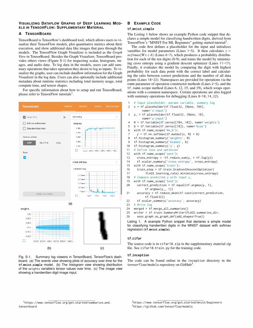
TensorBoard is Tensorflow’s dashboard tool, which allows users to vi-sualize their TensorFlow models, plot quantitative metrics about theirexecution, and show additional data like images that pass through themodels. The TensorFlow Graph Visualizer is included as the GraphView in TensorBoard. Besides the Graph Visualizer, TensorBoard pro-vides others views (Figure S-1) for inspecting scalar, histogram, im-ages, and audio data. To log data in the models, users can add sum-mary operations that takes operation they desire to log as inputs. To vi-sualize the graphs, user can include dataflow information for the GraphVisualizer in the log data. Users can also optionally include additionalmetadata about runtime statistics including total memory usage, totalcompute time, and tensor shapes.

For specific information about how to setup and run TensorBoard,please refer to TensorFlow tutorials1.

(b)

(a)

(c)

Fig. S-1. Summary log viewers in TensorBoard, TensorFlow’s dash-board. (a) The events view showing plots of accuracy over time for thetf mnist simple model. (b) The histogram view showing distributionof the weights variable’s tensor values over time. (c) The image viewshowing a handwritten digit image input.

1https://www.tensorflow.org/get started/summaries andtensorboard

B EXAMPLE CODE

tf mnist simple

The Listing 1 below shows an example Python code snippet that de-clares a simple model for classifying handwritten digits, derived fromTensorFlow’s “MNIST For ML Beginners” getting started tutorial2.

The code first defines a placeholder for the input and initializesvariables for model parameters (Lines 1-5). It then calculates y =so f tmax(Wx+b) (Lines 6-7), which produces a probability distribu-tion for each of the ten digits (0-9), and trains the model by minimiz-ing cross entropy using a gradient descent optimizer (Lines 11-17).Finally, it evaluates the model by comparing the digit with highestprobability for each data point with the correct label and calculat-ing the ratio between correct predictions and the number of all datapoints (Lines 18-22). Namespaces are provided for operations via thename parameter of operation constructor methods (Lines 2-5), and thetf.name scope method (Lines 6, 12, 15, and 19), which wraps oper-ations with a common namespace. Certain operations are also loggedwith summary operations for debugging (Lines 8-10,14,22).

1 # Input placeholder, params variable, summary log2 x = tf.placeholder(tf.float32, [None, 784],

name='x-input')3 y_ = tf.placeholder(tf.float32, [None, 10],

name='y-input')4 W = tf.Variable(tf.zeros([784, 10]), name='weights')5 b = tf.Variable(tf.zeros([10]), name='bias')6 with tf.name_scope('Wx_b'):7 y = tf.nn.softmax(tf.matmul(x, W) + b)8 tf.histogram_summary('weights', W)9 tf.histogram_summary('biases', b)10 tf.histogram_summary('y', y)11 # Define loss and optimizer12 with tf.name_scope('xent'):13 cross_entropy = -tf.reduce_sum(y_ * tf.log(y))14 tf.scalar_summary('cross entropy', cross_entropy)15 with tf.name_scope('train'):16 train_step = tf.train.GradientDescentOptimizer(17 FLAGS.learning_rate).minimize(cross_entropy)18 # Compare predicted y with input y_19 with tf.name_scope('test'):20 correct_prediction = tf.equal(tf.argmax(y, 1),

tf.argmax(y_, 1))21 accuracy = tf.reduce_mean(tf.cast(correct_prediction,

tf.float32))22 tf.scalar_summary('accuracy', accuracy)23 # Write log24 merged = tf.merge_all_summaries()25 writer = tf.train.SummaryWriter(FLAGS.summaries_dir,26 sess.graph.as_graph_def(add_shapes=True))

Listing 1. A example Python snippet that declares a simple modelfor classifying handwritten digits in the MNIST dataset with softmaxregression (tf mnist simple).

tf cifar

The source code is in cifar10.zip in the supplementary material zipfile. See cifar10 train.py for the training code.

tf inception

The code can be found online in the inception directory in thetensorflow/models repository on GitHub3.

2https://www.tensorflow.org/get started/mnist/beginners3https://github.com/tensorflow/models