visual tracking using kernel projected measurement and log-polar transformation

International Journal of Robotics, Vol. 4, No. 1, 1-11 (2015) / F. Bakhshande, H. D. Taghirad

* Corresponding author, Tel: +982188469084

1

Visual Tracking using Kernel Projected

Measurement and Log-Polar Transformation

Fateme Bakhshandea, Hamid D. Taghiradb,*

a Advanced Robotics and Automated Systems (ARAS), Industrial Control Center of Excellence (ICCE), Faculty of Electrical and Computer

Engineering, K. N. Toosi University of Technology, E-mail: [email protected]. b Advanced Robotics and Automated Systems (ARAS), Industrial Control Center of Excellence (ICCE), Faculty of Electrical and Computer

Engineering, K. N. Toosi University of Technology, E-mail: [email protected]

A R T I C L E I N F O A B S T R A C T Article history:

Received: December 15, 2014.

Received in revised form:

April 24, 2015. Accepted: May 29, 2015.

Visual Servoing is generally contained of control and feature tracking. Study of

previous methods shows that no attempt has been made to optimize these two parts

together. In kernel based visual servoing method, the main objective is to combine

and optimize these two parts together and to make an entire control loop. This main

target is accomplished by using Lyapanov theory. A Lyapanov candidate function is

formed based on kernel definition such that the Lyapanov stability can be verified.

The implementation is done in four degrees of freedom and Fourier transform is used

for decomposition of the rotation and scale directions from 2D translation. In the

present study, a new method in scale and rotation correction is presented. Log-Polar

Transform is used instead of Fourier transform for these two degrees of freedom.

Tracking in four degrees of freedom is synthesized to show the visual tracking of an

unmarked object. Comparison between Log-Polar transform and Fourier transform

shows the advantages of the presented method. KBVS based on Log-Polar transform

proposed in this paper, because of its robustness, speed and featureless properties.

Keywords:

Visual Servoing

Lyapanov Function Log-Polar Transform

Fourier Transform

1. Introduction

Visual servoing is commonly used for utilizing visual

feedbacks to control a robot [1]. Visual servoing (VS)

involves moving either a camera or the camera’s visual

target. The main purpose of VS is to track an object in an

unknown environment and to converge the target image

to a known desired image. In general, visual servoing

consists of two parts: feature tracking and control; in

addition, these two parts usually work separately in the

close-loop system which uses the vision as the underlying

parcel of the loop. VS is usually done without tracking

and control optimization. When the robot or object

moves, features that are extracted from the image are used

as the feedback signal, and control sequence is generated

based on these features. Therefore, the problem can be

divided into two sub-problems. By this separation, tuning

the whole system together is almost impossible. Kernel

Based Visual Servoing (KBVS) is presented in this paper

to optimize the VS method and to solve the two sub-

problems together. The presented method has some

superiorities over previous methods such as position-

based and image-based visual servoing [2], [3], 2 1/2 D

visual servoing [4] and other advanced methods [5], [6].

In all featureless methods the computational factors

decrease because of using all features in the image

without shrinking the image into limited extracted

features. Extracting features from an image usually

requires more computation and also decreases the speed

of convergence. KBVS uses the image signal or other

transformed image directly to optimize the close-loop

system. Spatial kernel-based tracking algorithm [7], [8],

[9], [10] is used in this method for designing the feedback

controller. The stability of control loop is proven by

Lyapunov theory.

Tracking based on kernel is used in [11], [12], [13] for the

first time. The most important part in KBVS is designing

the kernel function which tunes the performance of

control and tracking part. These functions have been

defined based on spatial weighted average of the image or

transformed image. Therefore, the minimal error of kernel

function is used for optimization during the tracking.

Swensen and Kallem rendered some kernels for 2D


2

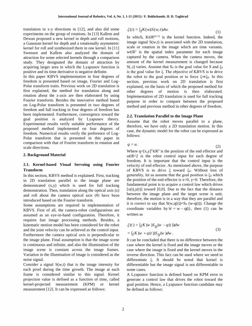
translation in x-y directions in [12], and also did some

experiments on the group of rotations. In [13] Kallem and

Dewan proposed a new kernel in depth and roll motions,

a Gaussian kernel for depth and a rotationally asymmetric

kernel for roll and synthesized them in one kernel. In [11]

Swensen and Kallem also analyzed the domain of

attraction for some selected kernels through a comparison

study. They designated the domain of attraction by

acquiring larger area in which the Lyapunov function is

positive and its time derivative is negative definite.

In this paper KBVS implementation in four degrees of

freedom is presented based on image, Fourier and Log-

Polar transform traits. Previous work on 2D translation is

first explained, the method for translation along and

rotation about the z-axis are then elaborated by using

Fourier transform. Besides the innovative method based

on Log-Polar transform is presented in two degrees of

freedom and full tracking in four degrees of freedom has

been implemented. Furthermore, convergence toward the

goal position is analyzed by Lyapunov theory.

Experimental results verify suitable performance of the

proposed method implemented on four degrees of

freedom. Numerical results verify the preference of Log-

Polar transform that is presented in this paper in

comparison with that of Fourier transform in rotation and

scale directions.

2. Background Material

2.1. Kernel-based Visual Servoing using Fourier

Transform

In this section, KBVS method is explained. First, tracking

in 2D translation parallel to the image plane are

demonstrated (x,y) which is used for full tracking

demonstration. Then, translation along the optical axis (z)

and roll about the camera optical axis (θ) have been

introduced based on the Fourier transform.

Some assumptions are required in implementation of

KBVS. First of all, the camera-robot configurations are

assumed as an eye-in-hand configuration. Therefore, it

requires fast image processing methods. Besides, a

kinematic motion model has been considered for the robot

and the joint velocity can be achieved as the control input.

Furthermore the camera optical axis is perpendicular to

the image plane. Final assumption is that the image scene

is continuous and infinite, and also the illumination of the

image scene is constant across the image frames.

Variation in the illumination of image is considered as the

noise signal.

Consider a signal S(w,t) that is the image intensity for

each pixel during the time growth. The image at each

frame is considered similar to this signal. Kernel

projection value is defined as a function of time, called

kernel-projected measurement (KPM) or kernel

measurement [12]. It can be expressed as follows:

.),()(=)( dwtwSwKIt (1)

In which, K∈R(n×1) is the kernel function. Indeed, the

image signal S(w,t) is associated with the 2D translation,

scale or rotation in the image which are time variants.

w∈R2 is the spatial index parameter for each image

captured by the camera. When the camera moves, the

amount of the kernel measurement is changed because

S(.,t) varies. Assume that S0 is the goal value for S and ξ0

is the goal value for ξ. The objective of KBVS is to drive

the robot to the goal position or to force ξ⇒ξ0. In this

section, previous work on 2D translation is first

explained, on the basis of which the proposed method for

other degrees of motion is then elaborated.

Implementation of 2D translation is used for full tracking

purpose in order to compare between the proposed

method and previous method in other degrees of freedom.

2.2. Translation Parallel to the Image Plane

Assume that the robot moves parallel to a plane,

therefore, we have only a 2D translation motion. In this

case, the dynamic model for the robot can be expressed as

follows:

.= uq (2)

Where q=[x,y]T∈R2 is the position of the end effector and

u∈R^2 is the robot control input for each degree of

freedom. It is important that the control input is the

velocity of end effector. As mentioned above, the purpose

of KBVS is to drive ξ toward ξ0. Without loss of

generality, let us assume that the goal position is ξ0 which

the position of the end effector is x=0, y=0. Therefore, the

fundamental point is to acquire a control law which drives

[x(t),y(t)] toward [0,0]. Due to the fact that the distance

between the image plane and the target scene is unit,

therefore, the motion is in a way that they are parallel and

it is correct to say that S(w,q(t))=S0 (w-q(t)). Change the

coordinate variables by q(t)w=w , then (1) can be

written as

( ) = ( ) ( ( ))0

= ( ( )) ( ) .0

t K w S w q t dwI

K w q t S w dwI

(3)

It can be concluded that there is no difference between the

case where the kernel is fixed and the image moves or the

case where the image is fixed and the kernel moves in the

reverse direction. This fact can be used where we need to

differentiate ξ. It should be noted that kernel is

differentiable but the image signal is not differentiable in

some cases.

A Lyapunov function is defined based on KPM error to

generate a control law that drives the robot toward the

goal position. Hence, a Lyapunov function candidate may

be defined as follows:


3

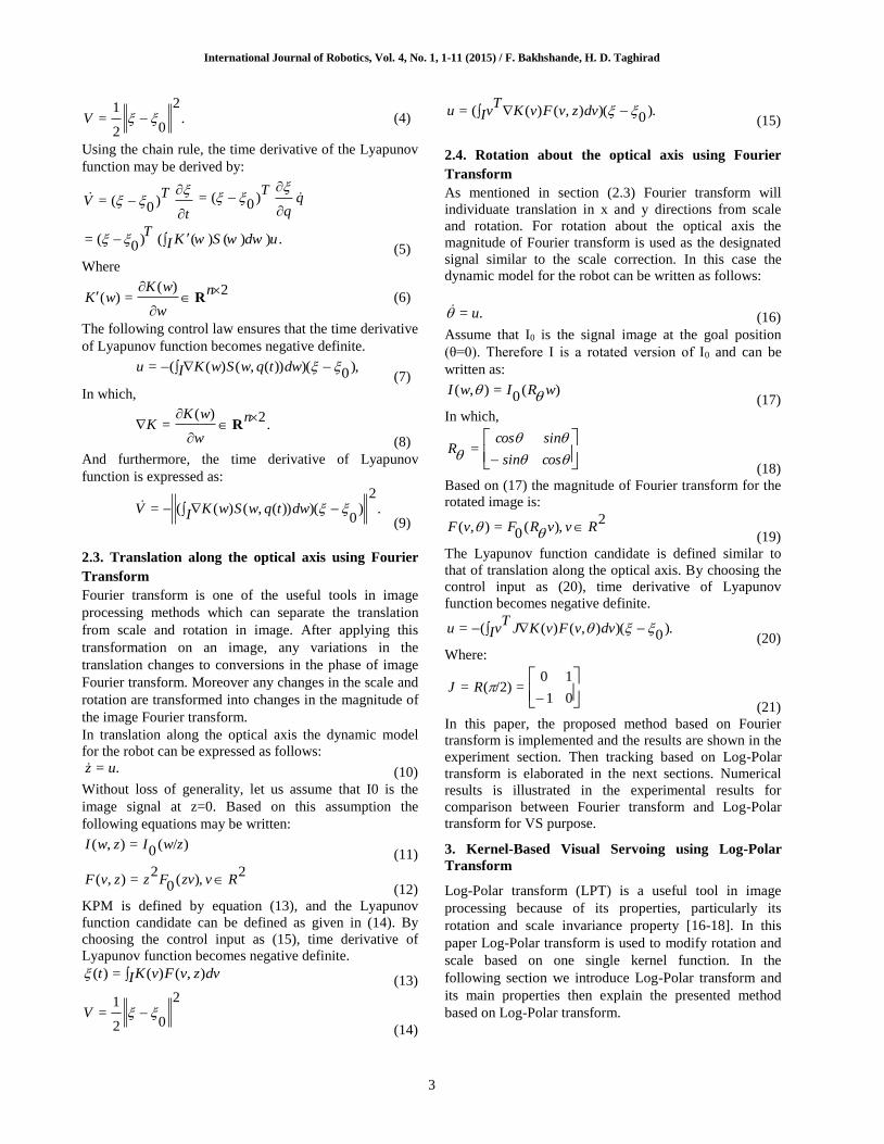
.2

02

1= V (4)

Using the chain rule, the time derivative of the Lyapunov

function may be derived by:

t

TV

)0(= q

q

T

)0(=

= ( ) ( ( ) ( ) ) .0

TK w S w dw uI

(5)

Where

2)(=)(

n

w

wKwK R

(6)

The following control law ensures that the time derivative

of Lyapunov function becomes negative definite.

),0)())(,()((= dwtqwSwKIu (7)

In which,

.2)(

=

n

w

wKK R

(8)

And furthermore, the time derivative of Lyapunov

function is expressed as:

.2

)0

)())(,()((= dwtqwSwKIV (9)

2.3. Translation along the optical axis using Fourier

Transform

Fourier transform is one of the useful tools in image

processing methods which can separate the translation

from scale and rotation in image. After applying this

transformation on an image, any variations in the

translation changes to conversions in the phase of image

Fourier transform. Moreover any changes in the scale and

rotation are transformed into changes in the magnitude of

the image Fourier transform.

In translation along the optical axis the dynamic model

for the robot can be expressed as follows:

.= uz (10)

Without loss of generality, let us assume that I0 is the

image signal at z=0. Based on this assumption the

following equations may be written:

)/(0=),( zwIzwI (11)

2),(

02

=),( RvzvFzzvF (12)

KPM is defined by equation (13), and the Lyapunov

function candidate can be defined as given in (14). By

choosing the control input as (15), time derivative of

Lyapunov function becomes negative definite.

dvzvFvKIt ),()(=)( (13)

2

02

1= V

(14)

).0

)(),()((= dvzvFvKT

vIu (15)

2.4. Rotation about the optical axis using Fourier

Transform

As mentioned in section (2.3) Fourier transform will

individuate translation in x and y directions from scale

and rotation. For rotation about the optical axis the

magnitude of Fourier transform is used as the designated

signal similar to the scale correction. In this case the

dynamic model for the robot can be written as follows:

.= u (16)

Assume that I0 is the signal image at the goal position

(θ=0). Therefore I is a rotated version of I0 and can be

written as:

)(0=),( wRIwI (17)

In which,

cossin

sincosR =

(18)

Based on (17) the magnitude of Fourier transform for the

rotated image is:

2),(

0=),( RvvRFvF

(19)

The Lyapunov function candidate is defined similar to

that of translation along the optical axis. By choosing the

control input as (20), time derivative of Lyapunov

function becomes negative definite.

).0

)(),()((= dvvFvKJT

vIu (20)

Where:

01

10=/2)(= RJ

(21)

In this paper, the proposed method based on Fourier

transform is implemented and the results are shown in the

experiment section. Then tracking based on Log-Polar

transform is elaborated in the next sections. Numerical

results is illustrated in the experimental results for

comparison between Fourier transform and Log-Polar

transform for VS purpose.

3. Kernel-Based Visual Servoing using Log-Polar

Transform

Log-Polar transform (LPT) is a useful tool in image

processing because of its properties, particularly its

rotation and scale invariance property [16-18]. In this

paper Log-Polar transform is used to modify rotation and

scale based on one single kernel function. In the

following section we introduce Log-Polar transform and

its main properties then explain the presented method

based on Log-Polar transform.


4

3.1. Log-Polar Transform

Log-Polar Transform is based on the human visual

system. Transformation of retinal image into its cortical

projection can be modeled by LPT [14]. It is mostly

utilizable in image registration and object recognition.

Indeed this mapping is non uniform. Therefore, LPT is a

nonlinear sampling method that registers an image from

Cartesian space to the polar space. In other words, LPT is

a 2D conformal transformation which transform

[x,y]⇒[φ,α] around the assigned center [xc,yc]. Therefore,

LPT can transform an image from Cartesian space to the

polar space as I(x,y)⇒ILP(φ,α). The mathematical

formulation of LPT is as follows [15].

2)(

2)(= cyycxx

baselog

(22)

).(1

=

cxx

cyytan

(23)

in which, (xc,yc) is the center pixel of the main image in

Cartesian coordinate, (x,y) illustrates sampling pixel in

the main image and (φ,θ) denotes the log-radius and the

angular position in Log-Polar coordinates. As shown in

the formulation of LPT and in the Fig. 1, it is obvious that

the radius of this transform treats exponentially by

increasing distance from the origin. As a result, angular

motion through this transformation remains constant from

Cartesian coordinate to the polar coordinate. [15]. Hence,

points near the origin are oversampled and by increasing

distance from the origin they will be undersampled.

Fig.1: LPT mapping: (a) a paradigm in Cartesian Coordinates, (b)

the result by applying Log-Polar Transform in radius and angular

direction.

3.2. Extract Rotation and Scale using Log-Polar

Transform

In this section we introduce our method which simplify

the definition of kernel and convert all degrees of

freedom into 2D translation. As shown in Fig. 1, the main

property of LPT is that rotation and scale in Cartesian

space is turned in shifting along the angular and radial

axes in the polar coordinate, respectively. This can be

proven based on LPT formulation as follows. Assume

that I(x,y) is the main image and L(x',y') is the

transformed image of I(x,y) that is rotated α degrees and

scaled by size of a [15]. Therefore,

y

x

cosasina

sinacosa

y

x

=

= , = x ax cos ay sin y ax sin ay cos

(24)

Consider that F(φ,θ) is the main image in Log-Polar

coordinate and G(φ',θ') is the rotated and scaled version

of it. Based on (24) we have:

2)(

2)(= yx

baselog

)(=22

= abase

lograbase

log

(25)

And also:

)(1

=x

ytan

= (26)

Therefore based on (25) and (26) it is realizable that

rotation and scale in the Cartesian space are transformed

into the displacement along the radial and angular axes in

the polar space.

In this paper LPT is applied on the main image and the

transformed image is used for rotation and scale

correction. Furthermore, for detecting movement in radial

and angular directions edge detection is applied on

transformed image. Furthermore, the edges are used for

tracking by using kernel based visual servoing method.

Therefore, the previous kernel function in x-y direction

can be used for this modification and it does not require

any new design for the kernel.

4. Asymptotic Stability

Up to here we have assumed a Lyapunov function

candidate that is positive definite and designed a control

input that just makes the derivative of Lyapunov function

negative semi-definite. Asymptotic stability requires

negative definiteness of V ̇ along the traversed trajectory.

Without loss of generality we assume that q0=0 is the goal

position. Therefore, our aim is to show that V is positive

definite and V ̇ is negative definite along the traversed

trajectory. To achieve that, use Taylor expansion of ξ(t)

about ξ0.


5

)2

()(0= qOtqq

(27)

)2

()(=0

qOtJq (28)

In equation (28) J is Jacobian matrix that may be defined

as follows:

dwtqwSwKIq

J ))(,()(==

(29)

In (27) O(q2) is higher order derivative terms of q. By

assuming a small neighborhood around the goal position,

higher order derivatives can be neglected from the Taylor,

and therefore, by using equation (28) Lyapunov function

and its derivative may be written as follows.

1= ( ) ( )

0 02

1 3= ( ) ( ) ( )

2

TV P

T Tq t J PJq t O q

(30)

PJT

JQ = (31)

)3

()()(= qOtqT

QQtqV (32)

In equation (31) P is a n×n matrix that is positive definite.

According to (30) and (32) if Jacobian matrix J∈R(n×p) (in

which n is the number of kernels and p is the dimension

of q(t)) is a full column rank, then Q is a full rank matrix

with p×p dimension. By this assumption, it can be

concluded that V is positive definite and V ̇ is negative

definite in a small neighborhood around the goal position,

and furthermore, they are zero at final destination point.

By this assumption asymptotic stability is proven just in a

small neighborhood around the goal position. In other

cases the higher order in (32) can not be neglected and

asymptotical stability is not proven. Experimental results

verify asymptotic stability behavior near the goal

position. The proposed method is not robust enough

against measurement noise therefore in some experiments

the uniformly ultimately bounded (UUB) stability could

be achieved instead of asymptotic stability.

5. Experimental Results

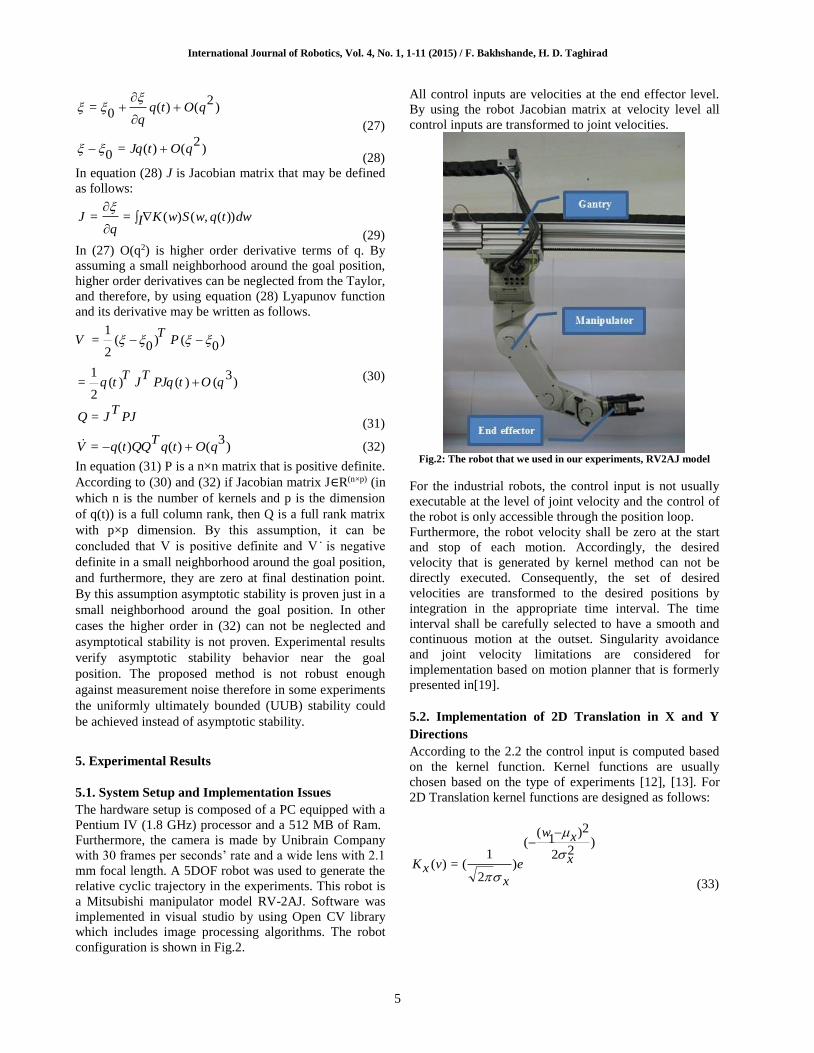
5.1. System Setup and Implementation Issues

The hardware setup is composed of a PC equipped with a

Pentium IV (1.8 GHz) processor and a 512 MB of Ram.

Furthermore, the camera is made by Unibrain Company

with 30 frames per seconds’ rate and a wide lens with 2.1

mm focal length. A 5DOF robot was used to generate the

relative cyclic trajectory in the experiments. This robot is

a Mitsubishi manipulator model RV-2AJ. Software was

implemented in visual studio by using Open CV library

which includes image processing algorithms. The robot

configuration is shown in Fig.2.

All control inputs are velocities at the end effector level.

By using the robot Jacobian matrix at velocity level all

control inputs are transformed to joint velocities.

Fig.2: The robot that we used in our experiments, RV2AJ model

For the industrial robots, the control input is not usually

executable at the level of joint velocity and the control of

the robot is only accessible through the position loop.

Furthermore, the robot velocity shall be zero at the start

and stop of each motion. Accordingly, the desired

velocity that is generated by kernel method can not be

directly executed. Consequently, the set of desired

velocities are transformed to the desired positions by

integration in the appropriate time interval. The time

interval shall be carefully selected to have a smooth and

continuous motion at the outset. Singularity avoidance

and joint velocity limitations are considered for

implementation based on motion planner that is formerly

presented in[19].

5.2. Implementation of 2D Translation in X and Y

Directions

According to the 2.2 the control input is computed based

on the kernel function. Kernel functions are usually

chosen based on the type of experiments [12], [13]. For

2D Translation kernel functions are designed as follows:

)22

2)1

((

)2

1(=)( x

xw

e

x

vxK

(33)


6

)22

2)2

((

)2

1(=)(

y

yw

e

y

vyK

(34)

In which, the parameters are set to μx=μy=-100, σx=σy=70,

while (w1,w2) is the image index. In Fig.3 three random

initials for 2D translation are tested. Suitable convergence

toward the goal is shown in this figure, while the mean

position errors of x and y are mentioned in Table 1.

Fig.3: Three experiment results in x-y directions. a) Performance in

x axis. b) Performance in y axis, c) convergence of KPM for 2d

translation

5.3. Implementation in four degrees of freedom by

using FFT

For implementation of KBVS, full tracking in four

degrees of freedom is required. Combination of four

degrees of freedom requires decomposition of 2D

translation from scale and rotation. As mentioned Fourier

transform is used for this purpose. Therefore, scale and

rotation compensation is done by the magnitude of

Fourier transform, and then the image signal is used for

tracking in 2D motion.

In this section, some experiments have been conducted to

validate the KBVS by using Fourier transform according

to the 2-3 and 2-4. We have done some experiments to

show the features of Fourier transform in KBVS method.

For illustration, some tests in scale and rotation directions

and the combination in four degrees of freedom have

been designed as follows:

1. Translation along and rotation about the optical axis by

computing Fourier transform.

2. Decomposition of 2D Translation from rotation and

scale corrections using the magnitude of Fourier

transform.

3. Combination of 3D translation (x,y,z) plus roll motion

about the optical axis by Fourier transforms.

5.3.1. Depth and Roll Motion Using FFT

Kernel functions for scale and rotation are selected,

respectively, as follows:

2(1/8)

=)(v

evzK

(35)

22

(1/8)21

(1/8)=)(

ve

vevK

(36)

In Fig. 4 five random initials for scale are tested. Suitable

convergence toward the goal is shown in this figure,

while the mean position errors of scale test are mentioned

in Table 2. Fig. 5 shows the five random initials to the

goal position for rotation test. Suitable convergence

toward the goal is shown in this figure, while the mean

position error of θ is mentioned in Table 2. It is obvious

in these figures that the performance of kernel based

visual servoing system is quite suitable for different initial

conditions. In order to verify similar results a compound

motion in all degrees of freedom is considered in the next

experiments.

Fig.4: Five experiment results in z directions. a) Performance in z

axis. b) Convergence of KPM for z axis using FFT

5.3.2. Decomposition of 2D Translation from rotation

and scale corrections


7

As mentioned before, for 2D translation the image

intensity is used directly but for scale and rotation the

magnitude of FFT is required. The purpose of this section

is to illustrate the effectiveness of FFT in the

decomposition of scale and rotation from 2D translation.

Note that in both experiments the magnitude of FFT is

independent from 2D translation, and therefore, in these

experiments the 2D translation error will not be directly

compensated.

Fig.5: Five experiment results in rotation about z axis a)

performance about θ. b) Convergence of KPM for θ using FFT

Fig. 6 illustrates the first experiment where the robot has

performed an x-y-z motion. As it is seen in the final

picture of this experiment by using FFT of the images in

the kernels, the z motion is compensated, but the x and y

remains unchanged. Similarly, Fig. 7 illustrates the

experiment result for a 3D motion in which in addition to

x-y motion rotation along z axis is considered. The same

decoupling in motion is clearly observed in the final

picture of the target, in which the rotation is compensated

for, while the x-y translation is not compensated.

Consequently magnitude of FFT is an effective tool to

decompose z and θ motions from 2D translation.

Therefore, it could be used for KBVS purposes.

5.3.3. 3D Translation + Roll Motion using FFT

For the final experiment we have considered a full 4D

motion, in which the 2D translation in x and y motion is

performed in addition to a translation along and a rotation

about z axis. In order to perform a full visual servoing

motion, first the scale and rotation is compensated by

using FFT in the kernels, and then the 2D translation is

performed. Fig. 8 illustrates the performance of this

experiment, in which the disparity between the final and

the goal positions are very small and hard to be observed

in this figure. This result verifies the effectiveness of the

decomposition method based on FFT image intensity. To

verify the result quantitatively, Fig. 9 and Fig. 10 are

given. Fig. 9 illustrates KPM for 2D translation, rotation

and scale, while Fig. 10 demonstrates the position error

norms in all four degrees of freedom. As it is shown in

these figures, the tracking errors in all 4 degrees of

freedom are relatively small, and remain in suitable range.

Relative comparison shows similar and better

performance in translational motion compared to that of

rotational performance.

Fig.6: Example images in a real environment. (a). Goal image. (b).

initial image with 2D translation and scale. (c). Final image with

scale compensation.

Fig.7: Example images in a real environment. (a). Goal image. (b).

initial image with 2D translation and rotation. (c). Final image with

rotation compensation.

Fig.8: Example images of a 4DOF trial in a real environment. The

goal, initial, final and disparity image.


8

Fig.9: Trial with random initial position, Convergence in X, Y, Z

and R motions.

Fig.10: Trial showing control to the goal image shown in Figure(8).

a). Convergence in KPM for X-Y. b). Convergence in KPM for Z.

c). Convergence in KPM for R.

5.4. Implementation in four degrees of freedom by

using LPT

In this section we try to implement the new KBVS

method based on Log-Polar transform to illustrate its

superiority to the Fourier transform. For this purpose two

tests have been designed and implemented on the robot as

follows:

1. Depth and roll compensation by computing Log-Polar

transform.

2. Combination of 3D translation (x,y,z) plus roll motion

about the optical axis by Log-Polar transforms.

The mean position errors of scale and rotation tests are

mentioned in Table 2 for more details.

5.4.1. Depth and Roll Motion by using LPT

In this part some experiments have been done on a real

object, which is a canister lid in a black background.

Some experiments have been performed on random initial

position around the goal image.

As mentioned LPT converts an image from Cartesian

space to the Polar space. By this transform rotation and

scale in Cartesian space convert to the 2D translation in

the polar space along the polar axes. Therefore, the 2D

translation kernel function can be used in this part.

Besides it should be considered that r is the log-radius in

the Log-Polar coordinates which treats exponentially by

increasing distance from the origin. Therefore, applying

2D translation kernel in this case terminates to

unfavorable results. To remedy this problem inverse of

the logarithm function is used in KPM, and since the

exponential function tends to infinity a tunable parameter

a is also considered. Eventually kernel functions are

selected as follows:

))2(2

2)1((

)2

1(=)2,1( z

zaw

e

e

z

wwzK

(37)

(38)

In (37) and (38) Kz and Kr are KPM for rotation and scale

respectively, μx=μy=-100 and σx=σy=70. These values

have been tuned during the experiments. Other

parameters that are tuned for the experiments are

controller gains and also a parameter in (37).

Firstly, we consider some initial position in which just the

scale translation along the optical axis is performed. Five

random initials have been considered and results are

shown in Fig. 11. Suitable convergence toward the goal is

shown in this figure, while the mean position error of

scale test is mentioned in Table 2. Besides we consider

rotation about the optical axis and performed for five

random initials positions. Results are shown in Fig. 12.

Suitable convergence toward the goal has been also

observed in this figure, while the mean position error of

scale test is mentioned in Table 2. Results in Table 2

show the advantages of using LPT in comparison with

FFT. As it is reported in this table, mean position errors

significantly decrease using Log-Polar transform.

One of the most important features of using Log-Polar

Transform is the combination of scale and rotation

correction. As mentioned before, this feature increases the

speed of convergence in compared with using Fourier

transform. In Fig. 13 three random initials are considered

while suitable convergence toward the goal is shown in

Fig. 14. It shows correction in roll and depth motion

simultaneously for a real object.


9

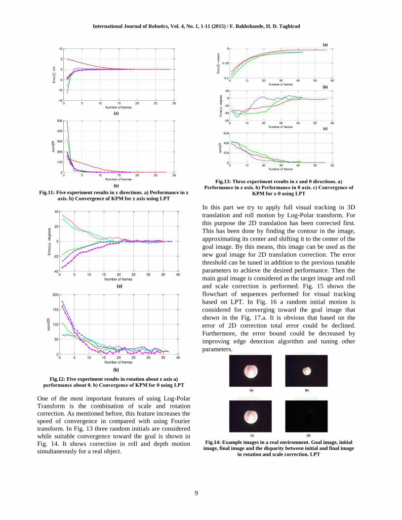
Fig.11: Five experiment results in z directions. a) Performance in z

axis. b) Convergence of KPM for z axis using LPT

Fig.12: Five experiment results in rotation about z axis a)

performance about θ. b) Convergence of KPM for θ using LPT

One of the most important features of using Log-Polar

Transform is the combination of scale and rotation

correction. As mentioned before, this feature increases the

speed of convergence in compared with using Fourier

transform. In Fig. 13 three random initials are considered

while suitable convergence toward the goal is shown in

Fig. 14. It shows correction in roll and depth motion

simultaneously for a real object.

Fig.13: Three experiment results in z and θ directions. a)

Performance in z axis. b) Performance in θ axis. c) Convergence of

KPM for z-θ using LPT

In this part we try to apply full visual tracking in 3D

translation and roll motion by Log-Polar transform. For

this purpose the 2D translation has been corrected first.

This has been done by finding the contour in the image,

approximating its center and shifting it to the center of the

goal image. By this means, this image can be used as the

new goal image for 2D translation correction. The error

threshold can be tuned in addition to the previous tunable

parameters to achieve the desired performance. Then the

main goal image is considered as the target image and roll

and scale correction is performed. Fig. 15 shows the

flowchart of sequences performed for visual tracking

based on LPT. In Fig. 16 a random initial motion is

considered for converging toward the goal image that

shown in the Fig. 17.a. It is obvious that based on the

error of 2D correction total error could be declined.

Furthermore, the error bound could be decreased by

improving edge detection algorithm and tuning other

parameters.

Fig.14: Example images in a real environment. Goal image, initial

image, final image and the disparity between initial and final image

in rotation and scale correction. LPT


10

Fig.15: Algorithm of full tracking based on LPT

Fig.16: Trial with random initial position, Convergence in X, Y, Z

and θ DOF, Convergence in KPM for z-θ and X-Y

Fig.17: Example images of a 4DOF trial in a real environment. (a).

Goal image. (b). Initial image. (c). Final image. (d). Disparity

between initial and final image in combination of 3D + roll motion.

Table 1. Results for KBVS method in 2D translation

10 trials with random initial

positions position error

mean position error of x (cm) 0.0205

mean position error of y (cm) 0.1202

Table 2. Comparison of Fourier transform and Log-Polar

transform in KBVS

10 trials with random initial positions position error

mean position error of z (cm)-FFT 0.5158

mean position error of θ (degrees)-FFT 0.2405

mean position error of z (cm)-LPT 0.0263

mean position error of θ (degrees)-LPT 0.0698

6. Conclusions

Kernel based visual servoing is a method in which

tracking is performed based on the KPM as the feedback

signal which is a weighted sum of the image. KBVS is a

featureless tracking method without the need to separate

tracking and control parts. Based on the KPM, a

Lyapanov function is given to verify asymptotic stability

of this method. Consequently the convergence of leading

an eye-in-hand robot to the goal position without any

feature tracking is verified in experiments. In this paper it

is proposed to use Fourier transform to decompose 2d

translational motion from the motion along, and rotation

about the z-axis. Experimental results verify effectiveness

of the proposed method in such decomposition. This idea

enables KBVS methods to be concurrently implemented

for four degrees of freedom. In the experiments, first the

translation along and the rotation about the z axis is

compensated by using FFT of image intensity, while at

the same time the other 2 degrees of translation are

compensated for with the ordinary kernel functions.

Besides Log-Polar transform has been introduced to

increase the accuracy and speed of convergence. This

purpose is done by converting the rotation and scale

directions from Cartesian space to the 2D translation in

the polar space. Besides compensation in rotation and


11

scale directions can be done simultaneously with one

kernel function. Final experimental results verify suitable

tracking performance for tracking an unmarked, and non

ideal object in a real environment. Comparison between

FFT and LPT shows the superiority of LPT performance

in KBVS method.

References

[1] A. Castano and S. Hutchinson, Visual compliance: Task

directed visual servo control, IEEE Transactions on

Robotics and Automation, 10 (1994) 334-342.

[2] S. Hutchinson, G.D. Hager, P.I. Corke, A tutorial on

visual servo control, 12 (1996) 651-670.

[3] W.J. Wilson, C.C. Williams Hulls, G.S. Bell, Relative

end-effector control using cartesian position based visual

servoing, IEEE Transactions on Robotics and

Automation, 12 (1996) 684-696.

[4] F. Chaumette and E. Malis, 2 1/2 D visual servoing: a

possible solution to improve image-based and position-

based visual servoings, IEEE International Conference

on Robotics and Automation, 1 (2000) 630-635.

[5] F. Chaumette and S. Hutchinson, Visual servo control,

part II: Advanced approaches, IEEE Robotics and

Automation Magazine, 14 (2007) 109-118.

[6] D. Kragic and H.I. Christensen, Technical report,

Computational Vision and Active Perception Laboratory,

(2002).

[7] D. Comaniciu, V. Ramesh,. Meerc, IEEE Transactions

on Pattern Analysis and Machine Intelligence, 25(5)

(2003) 564-575.

[8] M. Dewan and G. Hager, Towards optimal kernel-based

tracking, Computer Vision and Pattern Recognition, 1

(2006) 618-625.

[9] Z. Fan, Y. Wu, M. Yang, Multiple collaborative kernel

tracking. In Proc. IEEE Conf. on Computer Vision and

Pattern Recognition , 2005.

[10] G.D. Hager, M. Dewan, C.V. Stewart, Multiple kernel

tracking with ssd, In Proceedings of the IEEE

Conference on Computer Vision and Pattern

Recognition, 1 (2004) 790-797.

[11] J. Swensen, V. Kallem, N. Cowan, Empirical

Characterization of Convergence Properties for Kernel-

based Visual Servoing, Visual Servoing via Advanced

Numerical Methods, Springer–Verlag, (2010) 23-38.

[12] V. Kallem, J.P. Swensen, M. Dewan, G.D. Hager, N.J.

Cowan, Kernel-Based Visual Servoing: Featureless

Control using Spatial Sampling Functions.

[13] V. Kallem, M. Dewan, J.P. Swensen, G.D Hager, N.J.

Cowan, Kernel-based visual servoing, In IEEE/RSJ

International . Conference. on Intelligent Robots and

System, (2007) 1975-1980.

[14] H. Araujo and J.M. Dias, "An introduction to the log-

polar mapping", Second Workshop on Cybernetic

Vision, pp. 139 - 144, 2002.

[15] R. Matungka, "Studies on Log-Polar Transform for

Image Registration and Improvements Using Adaptive

Sampling and Logarithmic Spiral", 2009.

[16] K. Palander and S.S. Brandt, "Epipolar geometry and

log-polar transform in wide baseline stereo matching",

International Conference on Pattern Recognition, pp. 1-4,

2008.

[17] R. Matungka, Y.F. Zheng and R.L.Ewing, "Image

registration using adaptive polar transform", IEEE

Transactions on Image Processing, 18, pp. 2340-2354,

2009.

[18] R. Montoliu, V.J. Traver and F. Pla,"Log-polar mapping

in generalized least-squares motion estimation",

Proccedings of 2002 IASTED International Conference

on Visualization, Imaging, and Image Processing

(VIIP’2002), pp. 656-661, 2002.

[19] H. Taghirad, M. Shahbazi, F. Atashzar and S.

Rayatdoost, "Singular Free Motion Planning in Visual

Servoing of Redundant Manipulators", Submitted to IET

Computer Vision.

Fateme Bakhshande has received her

B.S. and M.S. degrees in electrical

engineering-control in 2009 and 2011

from K. N. Toosi University of

Technology, Tehran, Iran. From 2009

to 2011, she was a member of the

Advanced Robotics and Automated

Systems team (ARAS) and worked on

the visual servoing.

She is currently working toward her Ph.D. degree at

Duisburg-Essen University in Germany.

Now, she is a member of SRS team at Duisburg-Essen

University and her research interest is robust and

nonlinear control.

Hamid D. Taghirad has received his

B.Sc. degree in mechanical engineering

from Sharif University of Technology,

Tehran, Iran, in 1989, his M.Sc. in

mechanical engineering in 1993, and

his Ph.D. in electrical engineering in

1997, both from McGill University,

Montreal, Canada. He is currently the

chairman of the Faculty of Electrical Engineering, and a

Professor with the Department of Systems and Control

and the Director of the Advanced Robotics and

Automated System (ARAS) at K.N. Toosi University of

Technology, Tehran, Iran. He is a senior member of

IEEE, and member of the board of Industrial Control

Center of Excellence (ICCE), at K.N. Toosi University of

Technology, editor in chief of Mechatronics Magazine,

and Editorial board of International Journal of Robotics:

Theory and Application and International Journal of

Advanced Robotic Systems. His research interest is

robust and nonlinear control applied to robotic systems.

http://saba.kntu.ac.ir/eecd/aras/index.htm

http://saba.kntu.ac.ir/eecd/aras/index.htm

visual tracking using kernel projected measurement and log-polar transformation

Documents