To appear in the SIGGRAPH conference proceedings

Visual Simulation of SmokeRonaldFedkiw

�StanfordUniversity

JosStam�

Aliaswavefront

HenrikWannJensen�

StanfordUniversity

Abstract

In this paper, we proposea new approachto numericalsmokesimulationfor computergraphicsapplications. The methodpro-posedhereexploits physicsuniqueto smoke in order to designanumericalmethodthat is both fast and efficient on the relativelycoarsegrids traditionally usedin computergraphicsapplications(as comparedto the much finer grids usedin the computationalfluid dynamicsliterature). We usethe inviscid Euler equationsinour model, sincethey areusually moreappropriatefor gasmod-eling and lesscomputationallyintensive thanthe viscousNavier-Stokesequationsusedby others.In addition,we introducea physi-cally consistentvorticity confinementtermto modelthesmallscalerolling featurescharacteristicof smoke that are absenton mostcoarsegrid simulations.Ourmodelalsocorrectlyhandlestheinter-actionof smoke with moving objects.

Keywords: Smoke, computationalfluid dynamics,Navier-Stokes equations,Euler

equations,Semi-Lagrangianmethods,stablefluids, vorticity confinement,participat-

ing media

1 Intr oduction

Themodelingof naturalphenomenasuchassmoke remainsachal-lengingproblemin computergraphics(CG). This is not surprisingsincethe motion of gasessuchas smoke is highly complex andturbulent.Visualsmoke modelshave many obviousapplicationsintheindustryincludingspecialeffectsandinteractivegames.Ideally,a goodCG smoke modelshouldboth be easyto useandproducehighly realisticresults.

Obviously the modelingof smoke and gasesis of importanceto other engineeringfields as well. More generally, the field ofcomputationalfluid dynamics(CFD)is devotedto thesimulationofgasesandotherfluidssuchaswater. Only recentlyhaveresearchersin computergraphicsstartedto excavatethe abundantCFD litera-turefor algorithmsthatcanbeadoptedandmodifiedfor computergraphicsapplications.Unfortunately, currentCGsmokemodelsareeithertoo slow or suffer from too muchnumericaldissipation.Inthis paperwe adapttechniquesfrom theCFD literaturespecificto�

Stanford University, GatesComputerScienceBldg., Stanford, CA94305-9020,fedkiw@cs.stanford.edu�

Alias wavefront,1218ThirdAve,8thFloor, Seattle,WA 98101,U.S.A.jstam@aw.sgi.com�

Stanford University, GatesComputerScienceBldg., Stanford, CA94305-9020,henrik@graphics.stanford.edu

theanimationof gasessuchassmoke. We proposea modelwhichis stable,rapid and doesn’t suffer from excessive numericaldis-sipation.This allows us to produceanimationsof complex rollingsmokeevenonrelatively coarsegrids(ascomparedto theonesusedin CFD).

1.1 Previous Work

Themodelingof smokeandothergaseousphenomenahasreceiveda lot of attentionfrom thecomputergraphicscommunityover thelasttwo decades.Earlymodelsfocusedonaparticularphenomenonandanimatedthesmoke’s densitydirectlywithoutmodelingits ve-locity [10, 15, 5, 16]. Additional detailwasaddedusingsolid tex-tureswhoseparameterswere animatedover time. Subsequently,randomvelocityfieldsbasedonaKolmogoroff spectrumwereusedto modelthecomplex motioncharacteristicof smoke [18]. A com-mon trait sharedby all of theseearly modelsis that they lack anydynamicalfeedback.Creatinga convincing dynamicsmoke simu-lation is a timeconsumingtaskif left to theanimator.

A morenaturalway to modelthemotionof smoke is to simulatethe equationsof fluid dynamicsdirectly. Kajiya andVon Herzenwerethe first in CG to do this [13]. Unfortunately, the computerpower availableat the time (1984)only allowed themto produceresultson very coarsegrids. Exceptfor somemodelsspecifictotwo-dimensions[21, 9], noprogresswasmadein this directionun-til the work of FosterandMetaxas[7, 6]. Their simulationsusedrelatively coarsegridsbut producedniceswirling smokemotionsinthree-dimensions.Becausetheir modelusesanexplicit integrationscheme,their simulationsareonly stableif thetime stepis chosensmall enough.This makestheir simulationsrelatively slow, espe-cially whenthefluid velocity is largeanywhere in thedomainof in-terest.To alleviatethis problemStamintroduceda modelwhich isunconditionallystableandconsequentlycouldberun at any speed[17]. This wasachievedusinga combinationof a semi-Lagrangianadvectionschemesandimplicit solvers. Becausea first orderinte-grationschemewasused,the simulationssufferedfrom too muchnumericaldissipation.Althoughtheoverallmotionlooksfluid-like,smallscalevorticestypicalof smoke vanishtoo rapidly.

Recently, Yngve et al. proposedsolving the compressiblever-sionof theequationsof fluid flow to modelexplosions[22]. Whilethe compressibleequationsare useful for modelingshockwavesand other compressiblephenomena,they introducea very stricttimesteprestrictionassociatedwith theacousticwaves.MostCFDpractitionersavoid thisstrictconditionby usingtheincompressibleequationswhenever possible.For that reason,we do not considerthe compressibleflow equations. Another interestingalternativewhichwedonotpursuein thispaperis theuseof latticegassolversbasedon cellularautomata[4].

1.2 Our Model

Our model was designedspecifically to simulategasessuch assmoke. Wemodelthesmoke’svelocitywith theincompressibleEu-ler equations.Theseequationsaresolvedusinga semi-Lagrangianintegrationschemefollowed by a pressure-Poissonequationasin[17]. This guaranteesthatour modelis stablefor any choiceof thetime step. However, one of our main contributions is a method

To appear in the SIGGRAPH conference proceedings

to reducethe numericaldissipationinherentin semi-Lagrangianschemes.� We achieve this by usinga techniquefrom the CFD lit-eratureknown as ”vorticity confinement”[20]. The basicidea isto inject theenergy lost dueto numericaldissipationbackinto thefluid usinga forcing term.This forceis designedspecificallyto in-creasethevorticity of theflow. Visually this keepsthesmoke aliveover time. This forcing termis completelyconsistentwith theEu-ler equationsin the sensethat it disappearsasthe numberof gridcellsis increased.In CFDthistechniquewasappliedto thenumeri-calcomputationof complex turbulentflow fieldsaroundhelicopterswhereit is not possibleto addenoughgrid pointsto accuratelyre-solvetheflow field. Thecomputationof theforceonly addsasmallcomputationaloverhead.Consequentlyour simulationsarealmostasfastastheone’s obtainedfrom thebasicStableFluidsalgorithm[17]. Our model remainsstableas long as the magnitudeof theforcing term is kept below a certainthreshold.Within this range,our time stepsare still ordersof magnitudehigher than the onesusedin explicit schemes.

Semi-Lagrangianschemesarevery popularin the atmosphericsciencescommunityfor modelinglarge scaleflows dominatedbyconstantadvectionwherelargetime stepsaredesired,seee.g.[19]for a review. We borrow from this literaturea higherorder inter-polation techniquethat further increasesthe quality of the flows.This techniqueis especiallyeffective whenmoving densitiesandtemperaturesthroughthevelocity field.

Finally, our model,like FosterandMetaxas’[6], is ableto han-dleboundariesinsidethecomputationaldomain.Therefore,weareable to simulatesmoke swirling aroundobjectssuchas a virtualactor.

Therestof thepaperis organizedasfollows. In thenext sectionwederiveourmodelfrom theequationsof fluid flow, andin section3 we discussvorticity confinement. In section4, we outline ourimplementation.In section5, we presentbothaninteractive andahigh quality photonmapbasedrendererto depictour smoke simu-lations. Subsequently, in section6, we presentsomeresults,whilesection7 concludesanddiscussesfuturework.

2 The Equations of Fluid Flow

At theoutset,weassumethatourgasescanbemodeledasinviscid,incompressible,constantdensityfluids. The effects of viscosityarenegligible in gasesespeciallyon coarsegridswherenumericaldissipationdominatesphysicalviscosityandmoleculardiffusion.When the smoke’s velocity is well below the speedof soundthecompressibilityeffectsarenegligible aswell, andtheassumptionofincompressibilitygreatlysimplifiesthenumericalmethods.Conse-quently, theequationsthatmodelthesmoke’s velocity, denotedby��� ����������� , are given by the incompressibleEuler equations[14] ��� � � � (1)� ���� � ���� � � ���!� �#"%$'&)(

(2)

Thesetwo equationsstatethat the velocity shouldconserve bothmass(Equation1) andmomentum(Equation2). Thequantity

"is

thepressureof thegasand&

accountsfor externalforces.Also wehave arbitrarily settheconstantdensityof thefluid to one.

As in [7, 6, 17] we solve theseequationsin two steps.First wecomputean intermediatevelocity field � � by solving Equation2over a time step * �

without thepressureterm� � �+�* � ������ �,� ��� $-&)((3)

After this stepwe force the field � � to be incompressibleusingaprojectionmethod[3]. This is equivalentto computingthepressure

from thefollowing Poissonequation�/.0" �21* � ��� � � (4)

with pureNeumannboundarycondition,i.e., 354376 �8� at a bound-arypointwith normal 9 . (Notethatit is alsostraightforwardto im-poseDirichlet boundaryconditionswherethepressureis specifieddirectly asopposedto specifyingits normalderivative.) Theinter-mediatevelocity field is thenmadeincompressibleby subtractingthegradientof thepressurefrom it�:�;� � � * � �#"<(

(5)

We alsoneedequationsfor the evolution of both the tempera-ture = andthesmoke’s density> . We assumethatthesetwo scalarquantitiesaresimplymoved(advected)alongthesmoke’s velocity� =��� � ���� � � � = � (6)� >��� � ���� � � � > ( (7)

Both the densityandthe temperatureaffect thefluid’s velocity.Heavy smoketendsto fall downwardsduetogravity whilehotgasestendto risedueto buoyancy. Weusea simplemodelto accountfortheseeffects by defining external forcesthat are directly propor-tional to thedensityandthetemperature&@?5A5BDC ���FE >HG $JI = � =LK�M ? � G � (8)

where G �N��O�P�H� 1 � pointsin the upward vertical direction, =LK�M ?is theambienttemperatureof theair and E and

Iaretwo positive

constantswith appropriateunitssuchthatEquation8 is physicallymeaningful. Note that when > �Q� and = � =LK�M ? , this force iszero.

Equations2, 6 and7 all containtheadvectionoperator���� �@� � .As in [17], wesolvethistermusingasemi-Lagrangianmethod[19].We solve thePoissonequation(Equation4) for thepressureusinganiterativesolver. Weshow in Section4 how thesesolverscanalsohandlebodiesimmersedin thefluid.

3 Vor ticity Confinement

Usually smoke andair mixturescontainvelocity fields with largespatialdeviationsaccompaniedbyasignificantamountof rotationaland turbulent structureon a variety of scales. Nonphysicalnu-mericaldissipationdampsout theseinterestingflow features,andthe goal of our new approachis to add them back on the coarsegrid. Onewayof addingthembackwouldbeto createarandomorpseudo-randomsmall scaleperturbationof theflow field usingei-thera heuristicor physicallybasedmodel.For example,onecouldgeneratea divergencefreevelocity field usinga Kolmogorov spec-trum andaddthis to thecomputedflow field to representthemiss-ing smallscalestructure(see[18] for someCG applicationsof theKolmogorov spectrum).While this providessmall scaledetail totheflow, it doesnot placethe small scaledetailsin thephysicallycorrectlocationswithin theflow field wherethesmallscaledetailsaremissing. Instead,the detailsareaddedin a haphazardfashionand the smoke can appearto be “alive”, rolling and curling in anonphysicalfashion. The key to realistic animationof smoke isto make it look like a passive naturalphenomenaasopposedto a“li ving” creaturemadeoutof smoke.

Our methodlooks for the locationswithin the flow field wheresmall scalefeaturesshouldbe generatedandaddsthe small scalefeaturesin theselocationsin a physicallybasedfashionthat pro-motesthepassive rolling of smoke thatgivesit therealisticturbu-lent look on a coarseCG grid. With unlimited computingpower,

2

To appear in the SIGGRAPH conference proceedings

w

uv

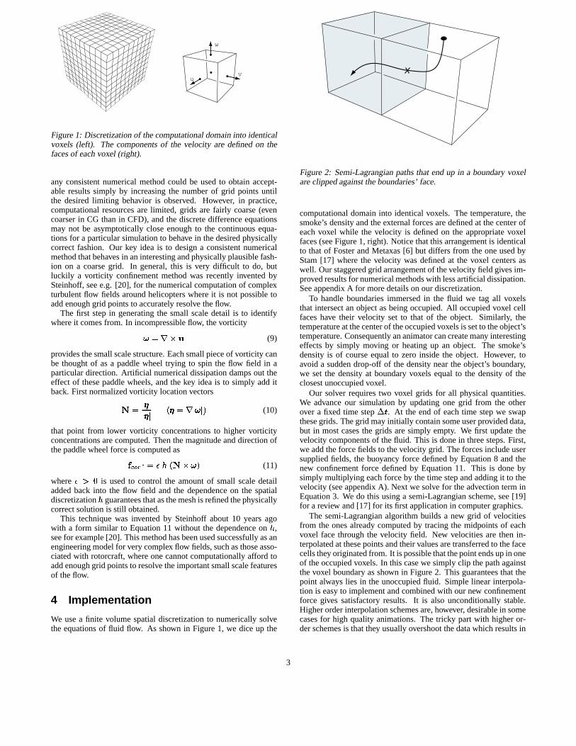
Figure1: Discretizationof thecomputationaldomaininto identicalvoxels (left). The componentsof the velocity aredefinedon thefacesof eachvoxel (right).

any consistentnumericalmethodcould be usedto obtain accept-able resultssimply by increasingthe numberof grid points untilthe desiredlimiting behavior is observed. However, in practice,computationalresourcesare limited, grids are fairly coarse(evencoarserin CG thanin CFD), andthediscretedifferenceequationsmay not be asymptoticallycloseenoughto the continuousequa-tionsfor a particularsimulationto behave in thedesiredphysicallycorrectfashion. Our key idea is to designa consistentnumericalmethodthatbehavesin aninterestingandphysicallyplausiblefash-ion on a coarsegrid. In general,this is very difficult to do, butluckily a vorticity confinementmethodwas recently inventedbySteinhoff, seee.g. [20], for thenumericalcomputationof complexturbulentflow fields aroundhelicopterswhereit is not possibletoaddenoughgrid pointsto accuratelyresolve theflow.

The first stepin generatingthe small scaledetail is to identifywhereit comesfrom. In incompressibleflow, thevorticityRRR � �TS � (9)

providesthesmallscalestructure.Eachsmallpieceof vorticity canbe thoughtof asa paddlewheel trying to spin the flow field in aparticulardirection. Artificial numericaldissipationdampsout theeffect of thesepaddlewheels,andthekey ideais to simply additback.First normalizedvorticity locationvectorsU �WVVVX VVV X VVV � � X RRR X � (10)

that point from lower vorticity concentrationsto higher vorticityconcentrationsarecomputed.Thenthemagnitudeanddirectionofthepaddlewheelforceis computedas&0YDB�Z\[ �;]_^` UaS RRR � (11)

where ]cba� is usedto control the amountof small scaledetailaddedback into the flow field and the dependenceon the spatialdiscretization guaranteesthatasthemeshis refinedthephysicallycorrectsolutionis still obtained.

This techniquewas inventedby Steinhoff about10 yearsagowith a form similar to Equation11 without the dependenceon ^ ,seefor example[20]. Thismethodhasbeenusedsuccessfullyasanengineeringmodelfor verycomplex flow fields,suchasthoseasso-ciatedwith rotorcraft,whereonecannotcomputationallyafford toaddenoughgrid pointsto resolvetheimportantsmallscalefeaturesof theflow.

4 Implementation

We usea finite volumespatialdiscretizationto numericallysolvetheequationsof fluid flow. As shown in Figure1, we diceup the

Figure2: Semi-Lagrangianpathsthatendup in a boundaryvoxelareclippedagainsttheboundaries’face.

computationaldomaininto identicalvoxels. The temperature,thesmoke’s densityandtheexternalforcesaredefinedat thecenterofeachvoxel while the velocity is definedon the appropriatevoxelfaces(seeFigure1, right). Noticethatthis arrangementis identicalto thatof FosterandMetaxas[6] but differs from theoneusedbyStam[17] wherethe velocity wasdefinedat the voxel centersaswell. Ourstaggeredgrid arrangementof thevelocityfield givesim-provedresultsfor numericalmethodswith lessartificial dissipation.SeeappendixA for moredetailson ourdiscretization.

To handleboundariesimmersedin the fluid we tag all voxelsthat intersectanobjectasbeingoccupied.All occupiedvoxel cellfaceshave their velocity set to that of the object. Similarly, thetemperatureatthecenterof theoccupiedvoxelsis setto theobject’stemperature.Consequentlyananimatorcancreatemany interestingeffects by simply moving or heatingup an object. The smoke’sdensityis of courseequalto zero inside the object. However, toavoid a suddendrop-off of thedensityneartheobject’s boundary,we set the densityat boundaryvoxels equalto the densityof theclosestunoccupiedvoxel.

Our solver requirestwo voxel grids for all physicalquantities.We advanceour simulationby updatingone grid from the otherover a fixed time step * �

. At the endof eachtime stepwe swapthesegrids.Thegrid mayinitially containsomeuserprovideddata,but in mostcasesthe grids aresimply empty. We first updatethevelocity componentsof thefluid. This is donein threesteps.First,weaddtheforcefieldsto thevelocitygrid. Theforcesincludeusersuppliedfields, the buoyancy force definedby Equation8 andthenew confinementforce definedby Equation11. This is donebysimply multiplying eachforceby thetime stepandaddingit to thevelocity (seeappendixA). Next we solve for theadvectionterminEquation3. We do this usinga semi-Lagrangianscheme,see[19]for a review and[17] for its first applicationin computergraphics.

The semi-Lagrangianalgorithmbuilds a new grid of velocitiesfrom the onesalreadycomputedby tracingthe midpointsof eachvoxel facethroughthe velocity field. New velocitiesare then in-terpolatedat thesepointsandtheirvaluesaretransferredto thefacecellsthey originatedfrom. It ispossiblethatthepointendsupin oneof theoccupiedvoxels. In this casewe simply clip thepathagainstthevoxel boundaryasshown in Figure2. This guaranteesthat thepoint alwayslies in theunoccupiedfluid. Simplelinear interpola-tion is easyto implementandcombinedwith our new confinementforce gives satisfactory results. It is also unconditionallystable.Higherorderinterpolationschemesare,however, desirablein somecasesfor high quality animations.The tricky part with higheror-derschemesis thatthey usuallyovershootthedatawhich resultsin

3

To appear in the SIGGRAPH conference proceedings

instabilities. In appendixB we provide a cubic interpolatorwhichdoesnotovershootthedata.

Finally we forcethevelocity field to conserve mass.As alreadystatedin section2, this involvesthesolutionof a Poissonequationfor the pressure(Equation4). The discretizationof this equationresultsin asparselinearsystemof equations.We imposefreeNeu-mannboundaryconditionsattheoccupiedvoxelsbysettingthenor-malpressuregradientequalto zeroat theoccupiedboundaryfaces.Thesystemof equationsis symmetric,andthemostnaturallinearsolver in this caseis the conjugategradientmethod.This methodis easyto implementandhasmuchbetterconvergencepropertiesthansimplerelaxationmethods.To improve the convergenceweusedanincompleteCholeskipreconditioner. Thesetechniquesareall quitestandardandwe refer the readerto thestandardtext [11]for moredetails.In practicewe foundthatonly about20 iterationsof this solver gave us visually acceptableresults. After the pres-sureis computed,we subtractits gradientfrom the velocity. SeeappendixA for theexactdiscretizationof theoperatorsinvolved.

After the velocity is updated,we advect both the temperatureand the smoke’s density. We solve theseequationsusingagainasemi-Lagrangianscheme.In this case,however, we tracebackthecentersof eachvoxel. The interpolationschemeis similar to thevelocity case.

5 Rendering

For every time step,our simulatoroutputsa grid that containsthesmoke’s density> . In thissectionwe presentalgorithmsto realisti-cally renderthesmoke undervariouslighting conditions.We haveimplementedbotha rapidhardwarebasedrendererasin [17] andahigh quality global illumination rendererbasedon thephotonmap[12]. The hardware basedrendererprovides rapid feedbackandallows ananimatorto get thesmoke to “look right”. Themoreex-pensive physics-basedrendereris usedat theendof theanimationpipelineto getproductionqualityanimationsof smoke.

We first briefly recall the additionalphysicalquantitiesneededto characterizetheinteractionof light with smoke. Theamountofinteractionis modeledby the inverseof the meanfree path of aphotonbeforeit collideswith the smoke andis called the extinc-tion coefficient dfe . Theextinction coefficient is directly relatedtothedensityof thesmoke throughanextinction cross-sectiongihDjPk :dfe � g h�jlk > . At eachinteractionwith thesmoke a photonis eitherscatteredor absorbed.The probability of scatteringis called thealbedom . A valueof thealbedonearzerocorrespondsto verydarksmoke, while a valuenearunity modelsbright gasessuchassteamandclouds.

In generalthe scatteringof light in smoke is mostly focusedintheforwarddirection.Thedistributionof scatteredlight is modeledthrougha phasefunction

" �n)� which givesthe probability that anincidentphotonis deflectedby anangle n . A convenientmodelforthephasefunctionis theHenyey-Greensteinfunction" �no�p� 1 �cq . 1 $ q . �-rsqit5u7v�no��wyx . � (12)

wherethe dimensionlessparameterq{z 1 modelsthe anisotropyof thescattering.Valuesnearunity of this parametercorrespondtogaseswhich scattermostly in the forward direction. We mentionthatthis phasefunctionis quitearbitraryandthatotherchoicesarepossible[1].

5.1 Hardware-Based Renderer

In our implementationof the hardware-basedrenderer, we followthe algorithm outlined in [17]. In a first pass,we computetheamountof light that directly reacheseachvoxel of the grid. This

is achievedusinga fastBresenhamline drawing voxel traversalal-gorithm[8]. Initially the transparenciesof eachray aresetto one( =L| K C � 1 ). Then,eachtimeavoxel is hit, thetransparency is com-putedfrom thevoxel’s density: =~} B j ���\�O���� gih�jlk ^f� , where ^ isthegrid spacing.Thenthevoxel’s radianceis setto� } B j � m ��� � ��� k 1 � = } B j � =L| K C �while thetransparency of therayis simplymultipliedby thevoxel’stransparency: = | K C � = | K C =~} B j . Sincethe transparency of theraydiminishesas it traversesthe smoke’s densitythis passcorrectlymimicstheeffectsof self-shadowing.

In asecondpasswerenderthevoxel grid from front to back.Wedecomposethevoxel grid into a setof two-dimensionalgrid-slicesalongthecoordinateaxismostalignedwith theviewing direction.Theverticesof thisgrid-slicecorrespondto thevoxel centers.Eachslice is thenrenderedasa setof transparentquads.Thecolor andopacityat eachvertex of a quadcorrespondto the radiance

� } B jandtheopacity 1 � = } B j , respectively, of thecorrespondingvoxel.Theblendingbetweenthedifferentgrid sliceswhenrenderedfromfront to backis handledby thegraphicshardware.

5.2 Photon Map Renderer

Realisticrenderingof smoke with a high albedo(suchaswaterva-por) requiresa full simulationof multiple scatteringof light insidethesmoke. This involvessolving the full volumerenderingequa-tion [2] describingthesteady-stateof light in thepresenceof par-ticipatingmedia. For this purposewe usethephotonmappingal-gorithmfor participatingmediaasintroducedin [12]. This is a twopassalgorithmin which thefirst passconsistsof building avolumephotonmapby emitting photonstowardsthe mediumandstoringtheseasthey interactwith themedium.We only storethephotonscorrespondingto indirectillumination.

In therenderingpasswe usea forwardray marchingalgorithm.We have found this to be superiorto the backward ray marchingalgorithmproposedin [12]. The forward ray marchingalgorithmallows for a moreefficientculling of computationsin smoke thatisobscuredby othersmoke. In additionit enablesamoreefficientuseof thephotonmapby allowing us to uselessphotonsin thequeryas the ray marchergetsdeeperinto the smoke. Our forward raymarcherhastheform�_� � � �H�R���� ���O��� � �O��� ���Ri� $'� �f�o���s�H� * � � ,�R � �� � �_� ���� �H�R��

(13)where� � � �_�;� �s��s� dfe)� � is theopticaldepth,

���is thefractionof

theinscatteredradiancethatis scatteredin direction �R , * � � b�� isthesizeof the   th step, � �)¡¢� ��� � $ * � � and � � � is a randomlychosenlocation in the   th segment. The factor

� �f�o���s�H�can be

consideredtheweightof the   th segment,andwe usethis valuetoadjusttherequiredaccuracy of thecomputation.

Thecontributiondueto in-scatteredradiance,�_£

, is givenby,�R � �� � �_� ���O�R���� mJdfe �~��¤f¥�¦ ��£ ���O�R �� � " � � � ���R � ���Ri� � R � (14)

We split the inscatteredradianceinto a singlescatteringterm,��§

,anda multiple scatteringterm,

��¨. The singlescatteringterm is

computedusing standardray tracing, and the multiple scatteringtermis computedusingthevolumeradianceestimatefrom thepho-tonmapby locatingthe   4 nearestphotons.Thisgives:

,�R � �� � ��¨ ���H�R���� � ©ª �¬« 4 ,�R � � " ���O�R � ���Ri�¥w)­<® w ((15)

Here « 4 is thepower of the"

th photonand ® is thesmallestsphereenclosingthe   4 photons.

4

To appear in the SIGGRAPH conference proceedings

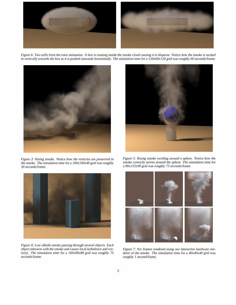
Figure6: Two stills from therotoranimation.A box is rotatinginsidethesmokecloudcausingit to disperse.Noticehow thesmoke is suckedin vertically towardstheboxasit is pushedoutwardshorizontally. Thesimulationtimefor a120x60x120grid wasroughly60seconds/frame.

Figure3: Risingsmoke. Noticehow thevorticiesarepreserved inthesmoke. Thesimulationtimefor a100x100x40grid wasroughly30seconds/frame.

Figure4: Low albedosmoke passingthroughseveralobjects.Eachobjectinteractswith thesmokeandcauseslocal turbulenceandvor-ticity. The simulationtime for a 160x80x80grid wasroughly 75seconds/frame.

Figure5: Risingsmoke swirling arounda sphere.Noticehow thesmoke correctlymovesaroundthesphere.Thesimulationtime fora90x135x90grid wasroughly75seconds/frame.

Figure7: Six framesrenderedusingour interactive hardwareren-dererof thesmoke. Thesimulationtime for a 40x40x40grid wasroughly1 second/frame.

5

To appear in the SIGGRAPH conference proceedings

Figure 8: Comparisonof linear interpolation(top) and our newmonotoniccubic interpolation(bottom).Thesimulationtime for a20x20x40grid wasroughly0.1 second/frame(linear)and1.8 sec-onds/frame(third order).

6 Results

This sectioncontainsseveral examplesof smoke simulations.Wehaverunmostof thesimulationsincludingtherenderingonadual-Pentium3-800or comparablemachine.Theimagesin Figures 3-6have beenrenderedat a width of 1024pixels using4 samplesperpixel. Thesephotonmaprenderingsweredoneusing1-2 millionphotonsin thevolumephotonmapandthe renderingtimesfor allthephotonmapimagesare20-45minutes.

Figure 3 is a simpledemonstrationof smoke rising. The onlyexternal force on the smoke is the naturalboyancy of the smokecausingit to rise. Notice how even this simplecaseis enoughtocreatearealisticandswirly apperanceof thesmoke. Figures4 and5 demonstratethatour solver correctlyhandlestheinteractionwithobjectsimmersedin thesmoke. Theseobjectsneednot beat rest.Figure 6 shows two stills from ananimationwherea rotatingcubeis insidea smoke cloud.Therotationof thecubecausesthesmoketo be pushedout horizontallyand sucked in vertically. The gridresolutionsandthecostof eachtime steparereportedin thefigurecaptions.

Figure 7 shows six framesof an animationrenderedusingourinteractive renderer. The renderingtime for eachframewas lessthana secondon a nVidia Quadrographicscard.Thespeed,whilenot real-time,allowed an animatorto interactively placedensitiesandheatsourcesin thesceneandwatchthesmokeraiseandbillow.

Finally, Figure 8 demonstratesthebenefitsof usinga higheror-der interpolantin thesemi-Lagrangianscheme.Thethreepictureson the top show theappearanceof falling smoke usinga linear in-terpolant,while the pictureson the bottomshow the samesmokeusingour new monotoniccubic interpolant.Clearly thenew inter-polationreducestheamountof numericaldissipationandproducessmoke simulationswith morefine detail.

7 Conc lusions

In this paperwe proposeda new smoke modelwhich is bothstableanddoesnot suffer from numericaldissipation.We achieved thisthroughthe useof a new forcing term that addsthe lost energybackexactlywhereit is needed.Wealsoincludedtheinteractionofobjectswith our smoke. We believe thatour modelis idealfor CGapplicationswherevisualdetailandspeedarecrucial.

Wethink thatvorticity confinementis a veryelegantandpower-ful technique.We areinvestigatingvariantsof this techniquecus-tom tailoredfor otherphenomenasuchasfire. We arealsoinvesti-gatingtechniquesto improve theinteractionof thesmoke with ob-jects. In our currentmodelobjectsmaysometimesbetoo coarselysampledon thegrid.

8 Ackno wledg ements

We would like to thank JohnSteinhoff (Flow Analysis Inc. andUTSI) and Pat Hanrahan(StanfordUniversity) for many helpfuldiscussions.Thework of thefirst authorwassupportedin partbyONR N00014-97-1-0027.The work of the last authorwas sup-portedby NSF/ITR (IIS-0085864)and DARPA (DABT63-95-C-0085).

A Discretization

We assumea uniform discretizationof spaceinto ¯ wvoxels with

uniform spacing . The temperatureandthe smoke’s densityarebothdefinedat thevoxel centersanddenotedby= £�° ±l° ²´³,µ�¶ > £�° ±l° ² � ·y�@¸o�y¹/� 1 � �5�5� � ¯ �respectively. The velocity on the otherhandis definedat the cellfaces.It isusualin theCFDliteratureto usehalf-wayindex notationfor this� £º¡p� x . ° ±l° ² �¬·¢�»�H� �5�5� � ¯ �Q¸)��¹¼� 1 � �5�s� � ¯ �� £�° ±l¡p� x . ° ² �¸%�»�H� �5�5� � ¯ �a·y��¹¼� 1 � �5�s� � ¯ �� £ ° ±l° ²\¡p� x . �¬¹¼�»�H� �5�s� � ¯ �N·��@¸%� 1 � �5�5� � ¯ (Using thesenotationswe cannow definesomediscreteoperators.Thedivergenceis definedas ��� �¢� £�° ±l° ² � � £º¡p� x . ° ±l° ² �c� £ ��� x . ° ±l° ² $� £ ° ±\¡¢� x . ° ² �½� £�° ±s��� x . ° ² $� £ ° ±l° ²\¡p� x . �c� £ ° ±l° ²,�<� x . ��¾,^while thediscretegradientsare(note

�#" �� " � � "f¿ � "fÀ ��� " � � £º¡¢� x . ° ±l° ² � " £º¡p��° ±l° ² � " £ ° ±l° ² ��¾7^<� " ¿ � £ ° ±\¡¢� x . ° ² � " £ ° ±\¡¢��° ² � " £�° ±l° ² ��¾,^<� "fÀ � £ ° ±l° ²\¡p� x . � " £ ° ±l° ²5¡¢� � " £ ° ±l° ² ��¾7^ (ThediscreteLaplacianis simply thecombinationof thedivergenceand the gradientoperators. The discreteversionof the vorticityRRR �8ÁR � �@R . �0R w � is definedasfollows. First we computethecell-centeredvelocitiesthroughaveragingÂ� £ ° ±l° ² � � £��<� x . ° ±l° ² $ � £º¡p� x . ° ±l° ² ��¾orÃ�Â� £ ° ±l° ² � � £ ° ± �<� x . ° ± $ � £�° ±l¡p� x . ° ± ��¾7rH�Â� £ ° ±l° ² � � £ ° ±l° ² ��� x . $ � £ ° ±l° ²5¡¢� x . ��¾7r (ThenR �£ ° ±l° ² � Â� £ ° ±\¡¢��° ² � Â� £�° ± ����° ² � Â� £�° ±l° ²5¡p� $ Â� £ ° ±l° ² ��� ��¾or,^<�R .£ ° ±l° ² � Â� £ ° ±l° ²\¡p� � Â� £�° ±l° ²,��� � Â� £Á¡¢��° ±l° ² $ Â� £��<��° ±l° ² ��¾7r7^<�R w£ ° ±l° ² � Â� £Á¡¢��° ±l° ² � Â� £��<��° ±l° ² � Â� £�° ±l¡p��° ² $ Â� £ ° ± �<��° ² ��¾7r7^ (

6

To appear in the SIGGRAPH conference proceedings

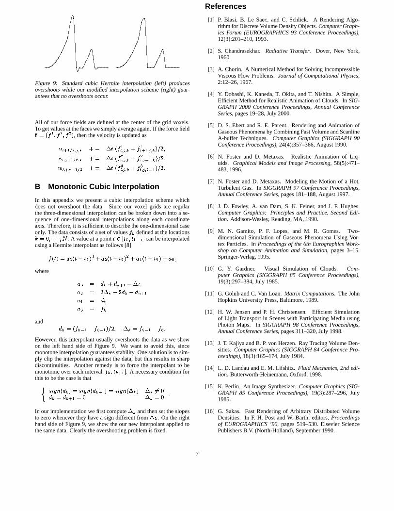
Figure 9: Standardcubic Hermite interpolation (left) producesovershootswhile our modified interpolationscheme(right) guar-anteesthatno overshootsoccur.

All of our force fields aredefinedat thecenterof thegrid voxels.To getvaluesat thefaceswesimplyaverageagain.If theforcefield& �ÄDÅ � �yÅ . �PÅ w � , thenthevelocity is updatedas� £º¡¢� x . ° ±l° ² $ � * � DÅ �£ ° ±l° ² $ Å �£Á¡¢��° ±l° ² ��¾7rH�� £ ° ±\¡¢� x . ° ² $ � * � DÅ .£ ° ±l° ² $ Å .£�° ±l¡p��° ² ��¾orÃ�� £ ° ±l° ²5¡¢� x . $ � * � DÅ w£ ° ±l° ² $ Å w£�° ±l° ²5¡p� ��¾7r (B Monotonic Cubic Interpolation

In this appendixwe presenta cubic interpolationschemewhichdoesnot overshootthe data. Since our voxel grids are regularthe three-dimensionalinterpolationcanbebroken down into a se-quenceof one-dimensionalinterpolationsalong eachcoordinateaxis.Therefore,it is sufficient to describetheone-dimensionalcaseonly. Thedataconsistsof asetof valuesÅ ² definedat thelocations¹¼�»�O� �5�5� � ¯ . A valueatapoint

�iÆcÇ � ² � � ²5¡¢��È canbeinterpolatedusingaHermiteinterpolantasfollows [8]Å� � ���ÊÉ w � � � ² � w $ É . � � � ² � .�$ É � � � � ² � $ ÉOË7�where É w � � ² $ � ²\¡p� � * ²É . � Ì * ² �+r � ² � � ²5¡¢�É � � � ²ÉOËÍ� Å ²and � ² ��DÅ ²5¡p� �-Å ² ��� ��¾orÃ� * ² �ÎÅ ²5¡¢� �JÅ ² (However, this interpolantusuallyovershootsthe dataaswe showon the left handside of Figure 9. We want to avoid this, sincemonotoneinterpolationguaranteesstability. Onesolutionis to sim-ply clip the interpolationagainstthe data,but this resultsin sharpdiscontinuities. Another remedyis to force the interpolantto bemonotonicover eachinterval

Ç � ² � � ²\¡p� È . A necessaryconditionforthis to bethecaseis thatϬР· q   � ² ��� Ð · q   � ²\¡p� �_� Ð · q   * ² � * ²ÒÑ�»�� ² � � ²\¡p� �»� * ² �»� (In our implementationwe first compute* ²

andthensettheslopesto zerowhenever they have a signdifferentfrom * ²

. On therighthandsideof Figure9, we show theour new interpolantappliedtothesamedata.Clearlytheovershootingproblemis fixed.

References

[1] P. Blasi, B. Le Saec,and C. Schlick. A RenderingAlgo-rithmfor DiscreteVolumeDensityObjects.Computer Graph-ics Forum (EUROGRAPHICS 93 Conference Proceedings),12(3):201–210,1993.

[2] S. Chandrasekhar. Radiative Transfer. Dover, New York,1960.

[3] A. Chorin. A NumericalMethodfor SolvingIncompressibleViscousFlow Problems.Journal of Computational Physics,2:12–26,1967.

[4] Y. Dobashi,K. Kaneda,T. Okita, andT. Nishita. A Simple,Efficient Methodfor RealisticAnimationof Clouds. In SIG-GRAPH 2000 Conference Proceedings, Annual ConferenceSeries, pages19–28,July2000.

[5] D. S. Ebert andR. E. Parent. RenderingandAnimation ofGaseousPhenomenaby CombiningFastVolumeandScanlineA-buffer Techniques. Computer Graphics (SIGGRAPH 90Conference Proceedings), 24(4):357–366,August1990.

[6] N. Foster and D. Metaxas. Realistic Animation of Liq-uids. Graphical Models and Image Processing, 58(5):471–483,1996.

[7] N. FosterandD. Metaxas. Modeling the Motion of a Hot,Turbulent Gas. In SIGGRAPH 97 Conference Proceedings,Annual Conference Series, pages181–188,August1997.

[8] J. D. Fowley, A. van Dam, S. K. Feiner, andJ. F. Hughes.Computer Graphics: Principles and Practice. Second Edi-tion. Addison-Wesley, Reading,MA, 1990.

[9] M. N. Gamito, P. F. Lopes, and M. R. Gomes. Two-dimensionalSimulationof GaseousPhenomenaUsing Vor-tex Particles. In Proceedings of the 6th Eurographics Work-shop on Computer Animation and Simulation, pages3–15.Springer-Verlag,1995.

[10] G. Y. Gardner. Visual Simulation of Clouds. Com-puter Graphics (SIGGRAPH 85 Conference Proceedings),19(3):297–384,July1985.

[11] G. GolubandC. VanLoan. Matrix Computations. TheJohnHopkinsUniversityPress,Baltimore,1989.

[12] H. W. Jensenand P. H. Christensen. Efficient Simulationof Light Transportin Sceneswith ParticipatingMedia usingPhotonMaps. In SIGGRAPH 98 Conference Proceedings,Annual Conference Series, pages311–320,July1998.

[13] J.T. Kajiya andB. P. von Herzen.RayTracingVolumeDen-sities. Computer Graphics (SIGGRAPH 84 Conference Pro-ceedings), 18(3):165–174,July1984.

[14] L. D. LandauandE. M. Lifshitz. Fluid Mechanics, 2nd edi-tion. Butterworth-Heinemann,Oxford,1998.

[15] K. Perlin. An ImageSynthesizer. Computer Graphics (SIG-GRAPH 85 Conference Proceedings), 19(3):287–296,July1985.

[16] G. Sakas. Fast Renderingof Arbitrary Distributed VolumeDensities. In F. H. PostandW. Barth, editors,Proceedingsof EUROGRAPHICS ’90, pages519–530.Elsevier SciencePublishersB.V. (North-Holland),September1990.

7

To appear in the SIGGRAPH conference proceedings

[17] J. Stam. StableFluids. In SIGGRAPH 99 Conference Pro-ceedings, Annual Conference Series, pages121–128,August1999.

[18] J. Stamand E. Fiume. Turbulent Wind Fields for GaseousPhenomena.In SIGGRAPH 93 Conference Proceedings, An-nual Conference Series, pages369–376,August1993.

[19] A. Staniforth and J. Cote. Semi-lagrangianintegrationschemesfor atmosphericmodels:A review. Monthly WeatherReview, 119:2206–2223,1991.

[20] J.Steinhoff andD. Underhill. Modificationof theeulerequa-tionsfor “vorticity confinement”:Applicationto thecomputa-tion of interactingvortex rings. Physics of Fluids, 6(8):2738–2744,1994.

[21] L. YaegerandC.Upson.CombiningPhysicalandVisualSim-ulation.Creationof thePlanetJupiterfor theFilm 2010.Com-puter Graphics (SIGGRAPH 86 Conference Proceedings),20(4):85–93,August1986.

[22] G. Yngve,J.O’Brien, andJ.Hodgins.Animatingexplosions.In SIGGRAPH 2000 Conference Proceedings, Annual Con-ference Series, pages29–36,July2000.

8