visual sample plan version 7.0 user's guide
TRANSCRIPT

UNCLASSIFIED PNNL-23211
UNCLASSIFIED
Visual Sample Plan
Version 7.0 User’s Guide
B.D. Matzke J.E. Wilson
L.L. Newburn S.T. Dowson
J.E. Hathaway L.H. Sego
L.M. Bramer B.A. Pulsipher
March 2014

UNCLASSIFIED
UNCLASSIFIED
DISCLAIMER
This report was prepared as an account of work sponsored by an agency of the
United States Government. Neither the United States Government nor any
agency thereof, nor Battelle Memorial Institute, nor any of their employees,
makes any warranty, express or implied, or assumes any legal liability or
responsibility for the accuracy, completeness, or usefulness of any
information, apparatus, product, or process disclosed, or represents that
its use would not infringe privately owned rights. Reference herein to any
specific commercial product, process, or service by trade name, trademark,
manufacturer, or otherwise does not necessarily constitute or imply its
endorsement, recommendation, or favoring by the United States Government
or any agency thereof, or Battelle Memorial Institute. The views and opinions
of authors expressed herein do not necessarily state or reflect those of the
United States Government or any agency thereof.
PACIFIC NORTHWEST NATIONAL LABORATORY
operated by
BATTELLE
for the
UNITED STATES DEPARTMENT OF ENERGY
under Contract DE-AC05-76RL01830
Printed in the United States of America
Available to DOE and DOE contractors from the
Office of Scientific and Technical Information,
P.O. Box 62, Oak Ridge, TN 37831-0062;
ph: (865) 576-8401
fax: (865) 576-5728
email: [email protected]
Available to the public from the National Technical Information Service,
U.S. Department of Commerce, 5285 Port Royal Rd., Springfield, VA 22161
ph: (800) 553-6847
fax: (703) 605-6900
email: [email protected]
online ordering: http://www.ntis.gov/ordering.htm

UNCLASSIFIED PNNL-23211
UNCLASSIFIED
Visual Sample Plan
Version 7.0 User’s Guide
B.D. Matzke J.E. Wilson
L.L. Newburn S.T. Dowson
J.E. Hathaway L.H. Sego
L.M. Bramer B.A. Pulsipher
March 2014
Prepared for the U.S. Department of Energy
under Contract DE-AC05-76RL01830
Pacific Northwest National Laboratory
Richland, Washington 99352

UNCLASSIFIED PNNL-23211
March 2014 UNCLASSIFIED Visual Sample Plan Version 7.0
iii
Abstract
This user's guide describes Visual Sample Plan (VSP) Version 7.0 and provides instructions for using the
software. VSP selects the appropriate number and location of environmental samples to ensure that the
results of statistical tests performed to provide input to risk decisions have the required confidence and
performance. VSP Version 7.0 provides sample-size equations or algorithms needed by specific
statistical tests appropriate for specific environmental sampling objectives. It also provides data quality
assessment and statistical analysis functions to support evaluation of the data and determine whether the
data support decisions regarding sites suspected of contamination. The easy-to-use program is highly
visual and graphic. VSP runs on personal computers with Microsoft Windows operating systems (XP,
Vista, Windows 7, and Windows 8). Designed primarily for project managers and users without expertise
in statistics, VSP is applicable to two- and three-dimensional populations to be sampled (e.g., rooms and
buildings, surface soil, a defined layer of subsurface soil, water bodies, and other similar applications) for
studies of environmental quality. VSP is also applicable for designing sampling plans for assessing
chem/rad/bio threat and hazard identification within rooms and buildings, and for designing geophysical
surveys for unexploded ordnance (UXO) identification.

UNCLASSIFIED PNNL-23211
March 2014 UNCLASSIFIED Visual Sample Plan Version 7.0
iv
Acronyms
ACS Attribute Compliance Sampling
AL Action Level or Action Limit
ANOVA Analysis of Variance
AWE U.K. Atomic Weapons Establishment
CDC U.S. Center for Disease Control
CI Confidence Interval
COG Course-Over-Ground
CS Collaborative Sampling
CSM Conceptual Site Model
DCGLw Derived Concentration Guideline Level for average concentrations over a wide area
DOD U.S. Department of Defense
DOE U.S. Department of Energy
DHS U.S. Department of Homeland Security
DPGD Decision Performance Goal Diagram
DQA Data Quality Assessment
DQO Data Quality Objectives
EPA U.S. Environmental Protection Agency
ESTCP Environmental Security Technology Certification Program
GIGO Garbage In, Garbage Out
GPS global positioning system
LBGR Lower Bound of the Gray Region
MARSSIM Multi-Agency Radiation Survey and Site Investigation Manual

UNCLASSIFIED PNNL-23211
March 2014 UNCLASSIFIED Visual Sample Plan Version 7.0
v
MI Multiple Increment
MK Mann-Kendall
MQO Measurement Quality Objectives
NFA no-futher-action
NIOSH National Institute for Occupational Safety and Health
OSL Optimum Segment Length
PCS Projected Coordinate System
PI Prediction Interval
RCRA Resource Conservation & Recovery Act of 1976
RTF rich text format
RI Remedial Investigation
RMSE Root Mean Square Error
RSS Ranked Set Sampling
RTF Rich Text Format
SE Standard Error
SERDP Strategic Environmental Research & Development Program
TOI Targets of Interest
UCL Upper Confidence Limit
UBGR Upper Bound of the Gray Region
UTL Upper Tolerance Limit
UTM Universal Transverse Mercator
UXO Unexploded ordnance
VSP Visual Sample Plan

UNCLASSIFIED PNNL-23211
March 2014 UNCLASSIFIED Visual Sample Plan Version 7.0
vi
WRS Wilcoxon Rank Sum
WSR Wilcoxon Signed Rank

UNCLASSIFIED PNNL-23211
March 2014 UNCLASSIFIED Visual Sample Plan Version 7.0
vii
Acknowledgments
We wish to thank the many sponsors from multiple US Government Agencies and the United Kingdom
Atomic Weapons Establishment, and the United Kingdom Government Decontamination Services for
their continued support of VSP developments. We thank current and former employees George Detsis,
Josh Silverman, and Rich Bush, U.S. Department of Energy, Dino Mattorano, Larry Kaelin, Doug
Maddox, and John Warren, U.S. Environmental Protection Agency, Randy Long, Teresa Lustig, Lance
Brooks, Chris Russell, and Don Bansleben, U.S. Department of Homeland Security, Anne Andrews, Herb
Nelson, and Jeff Marqusee, U.S. Department of Defense (SERDP/ESTCP), Karl Sieber and Stan
Shulman, U.S. Center for Disease Control NIOSH, and Steve Wilcox and Sara Casey, our UK sponsors
and collaborators, for their past and continued support and guidance on the development of many modules
in VSP. We also wish to thank Rebecca Blackmon, Bill Ingersoll, Fred McLean, Ed Hartzog, David
Bottrell, and Larry Zaragoza for their past support. We thank Sean McKenna and Barry Roberts, Sandia
National Laboratory, for their significant contributions to the geostatistical methods for unexploded
ordnance sites. Special thanks are extended also to individuals in the Statistical Sciences and Sensor
Analytics Group at Pacific Northwest National Laboratory: Kevin Anderson for statistical expertise; Ryan
Orr for his efforts in quality assurance; Brett Amidan and Patrick Paulson for their assistance on projects,
and Connie Martin for her project financial accounting support We also want to especially thank Steve
Wilcox for the continued beta testing and recommended improvements, and Dick Gilbert, Jim Davidson,
and Nancy Hassig for their past contributions to VSP. The authors are pleased to acknowledge the
contribution from the developers of ProUCL on some of the statistical analysis algorithms.

March 2014 Visual Sample Plan Version 7.0 vii
Contents
Abstract ........................................................................................................................................................ iii
Acknowledgments ........................................................................................................................................ vi
1.0 Introduction ......................................................................................................................................... 1.1
1.1 What is Visual Sample Plan? ....................................................................................................... 1.1
1.2 Installation and System Requirements ......................................................................................... 1.2
1.3 Overview of VSP ......................................................................................................................... 1.3
1.4 How Do I Use VSP to Provide a Defensible Sampling Plan? ..................................................... 1.5
1.5 What’s New in VSP 6.0? ............................................................................................................. 1.5
2.0 Mechanics of Running VSP ................................................................................................................ 2.1
2.1 Getting Started and Navigational Aids ........................................................................................ 2.1
2.2 Setting Up a Map ......................................................................................................................... 2.2
2.2.1 Importing a Site Map from a File .................................................................................... 2.3
2.2.2 Importing a Site Map File in the VSP Format ................................................................. 2.4
2.2.3 Draw Map Using VSP Drawing Tools ............................................................................ 2.4
2.2.4 Working with Maps ......................................................................................................... 2.5
2.2.5 Additional Map Features ................................................................................................. 2.7
2.3 Sample Areas in VSP ................................................................................................................... 2.8
2.3.1 Creating a Sample Area ................................................................................................... 2.8
2.3.2 Selecting or Deselecting Sample Areas ......................................................................... 2.12
2.3.3 Deleting Selected Sample Areas .................................................................................... 2.12
2.3.4 Sample Area Parameters ................................................................................................ 2.13
2.3.5 Extended Sample Area Topics ....................................................................................... 2.15
2.4 Map Layers and Properties in VSP ............................................................................................ 2.16
2.4.1 Map Lines ...................................................................................................................... 2.17
2.4.2 Sample Areas ................................................................................................................. 2.17
2.4.3 View Settings ................................................................................................................. 2.18
2.4.4 Properties Bar ................................................................................................................ 2.18
2.5 Individual Samples (Importing, Exporting, Removing, and Labeling Them as Historical) ...... 2.19
2.5.1 Data Entry Sub-Page ...................................................................................................... 2.20
2.5.2 Other Ways of Importing Samples ................................................................................ 2.25
2.5.3 Historical Samples ......................................................................................................... 2.27
2.5.4 Another Way of Exporting Sampling Locations ............................................................ 2.27

March 2014 Visual Sample Plan Version 7.0 viii
2.5.5 Removing Sampling Locations ...................................................................................... 2.27
2.5 Rooms and Buildings in VSP .................................................................................................... 2.28
2.6.1 Drawing a Room ............................................................................................................ 2.29
2.6.2 Extended Room Features ............................................................................................... 2.33
2.6.3 Extended Room Features ............................................................................................... 2.34
2.6.4 Furniture and Stairs ........................................................................................................ 2.39
2.7 Surface Overlays ........................................................................................................................ 2.47
2.8 Saving a VSP File ...................................................................................................................... 2.47
2.9 Help ............................................................................................................................................ 2.47
2.9.1 Expert Mentor………………………………………………………………………….2.48
3.0 Sampling Plan Development Within VSP .......................................................................................... 3.1
3.1 Sampling Plan Type Selection ..................................................................................................... 3.1
3.1.1 Defining the Purpose/Goal of Sampling .......................................................................... 3.1
3.1.2 Selecting a Sampling Design ........................................................................................... 3.4
3.2 DQO Inputs and Sample Size ...................................................................................................... 3.8
3.2.1 Compare Average to a Fixed Threshold .......................................................................... 3.9
3.2.2 Compare Average to Reference Average....................................................................... 3.19
3.2.3 Estimate the Mean ......................................................................................................... 3.26
3.2.4 Construct Confidence Interval on Mean ........................................................................ 3.36
3.2.5 Locating a Hot Spot ....................................................................................................... 3.38
3.2.6 Show That At Least Some High % of the Sampling Area is Acceptable ...................... 3.41
3.2.7 Discover Unacceptable Areas With High Confidence ................................................... 3.48
3.2.8 Combined Average and Individual Measurement Criteria ............................................ 3.50
3.2.9 Detecting a Trend ........................................................................................................... 3.50
3.2.10 Identify Sampling Redundancy ...................................................................................... 3.54
3.2.11 Add Sampling Locations ............................................................................................... 3.66
3.2.12 Compare Proportion to Fixed Threshold ....................................................................... 3.67
3.2.13 Compare Proportion to Reference Proportion ............................................................... 3.68
3.2.14 Construct Confidence Interval on Proportion ................................................................ 3.68
3.2.15 Estimate the Proportion ................................................................................................. 3.70
3.2.16 Establish Boundary of Contamination ........................................................................... 3.70
3.2.17 UXO Guide .................................................................................................................... 3.74
3.2.18 Find UXO Target Areas ................................................................................................. 3.74
3.2.19 Post Remediation Verification Sampling ....................................................................... 3.74
3.2.20 Remedial Investigation .................................................................................................. 3.74
3.2.21 Sampling Within Buildings ........................................................................................... 3.75
3.2.22 Radiological Transect Surveying ................................................................................... 3.76
3.2.23 Item Sampling ................................................................................................................ 3.77
3.2.24 Non-statistical Sampling Approach ............................................................................... 3.77

March 2014 Visual Sample Plan Version 7.0 ix
3.2.25 Last Design .................................................................................................................... 3.78
4.0 Assessment of Sampling Plans ........................................................................................................... 4.1
4.1 Display of Sampling Design on the Map: MAP VIEW button or View > Map ......................... 4.1
4.2 Display of Cost of Design ............................................................................................................ 4.2
4.3 Display of Performance of Design: GRAPH VIEW button or View > Graph ........................... 4.2
4.3.1 Performance of Design for Sampling Goal: Compare Average to a Fixed
Threshold ......................................................................................................................... 4.2
4.3.2 Performance of Design for Sampling Goal: Construct Confidence Interval
on the Mean ..................................................................................................................... 4.6
4.3.3 Performance of Design for Sampling Goal: Comparing a Proportion to
a Fixed Threshold ............................................................................................................ 4.7
4.3.4 Performance of Design for Sampling Goal: Compare Average to Reference
Average ............................................................................................................................ 4.8
4.3.5 Performance of Design for Sampling Goal for Hot Spot Problem ................................ 4.10
4.3.6 Performance of Design for Sampling Goal of Compare Proportion to a
Reference Proportion ..................................................................................................... 4.11
4.3.7 Performance of Design for Sampling Goal of Establish Boundary of
Contamination ................................................................................................................ 4.13
4.4 Display of the Report ................................................................................................................. 4.14
4.5 Display of Coordinates .............................................................................................................. 4.21
4.6 Multiple Displays ....................................................................................................................... 4.22
4.7 Room View ................................................................................................................................ 4.23
4.8 3D View ..................................................................................................................................... 4.23
5.0 Extended Features of VSP .................................................................................................................. 5.1
5.1 Tools ............................................................................................................................................ 5.1
5.1.1 Largest Unsampled Spot .................................................................................................. 5.1
5.1.2 Reset Sampling Design .................................................................................................... 5.3
5.1.3 Measure Distance ............................................................................................................. 5.3
5.1.4 Make Sample Labels ........................................................................................................ 5.3
5.1.4 Make Transect Labels ...................................................................................................... 5.4
5.1.6 Analyze Data .................................................................................................................... 5.4
5.1.7 Geostatistical Analysis ..................................................................................................... 5.5
5.1.8 Correlate Analytes ........................................................................................................... 5.5
5.1.9 Group Comparison / ANOVA ......................................................................................... 5.7
5.2 Options ....................................................................................................................................... 5.10
5.2.1 Random Numbers .......................................................................................................... 5.10
March 2014 Visual Sample Plan Version 7.0 x
5.2.2 Sample Placement .......................................................................................................... 5.11
5.2.3 Graph ............................................................................................................................. 5.13
5.2.4 Measurement Quality Objectives (MQOs) .................................................................... 5.14
5.2.5 Sensitivity Analysis ....................................................................................................... 5.18
5.2.6 Coordinate Digits ........................................................................................................... 5.20
5.2.7 Waypoint Distance ......................................................................................................... 5.20
5.2.8 Preferences ..................................................................................................................... 5.20
5.3 View Menu ................................................................................................................................ 5.22
5.4 The Cost Tab: Setting Up Sampling Costs – Inputs for the General Screen ............................ 5.23
5.5 Multiple Areas to be Sampled .................................................................................................... 5.24
5.6 Data Analysis ............................................................................................................................. 5.24
5.6.1 Data Entry ...................................................................................................................... 5.26
5.6.2 Summary Statistics ........................................................................................................ 5.26
5.6.3 Tests ............................................................................................................................... 5.27
5.6.4 Plots ............................................................................................................................... 5.29
6.0 Room Features in VSP ........................................................................................................................ 6.1
6.1 Room Creation and Manipulation ................................................................................................ 6.1
6.1.1 Creating a Room from a Sample Area ............................................................................. 6.1
6.1.2 Drawing a Room .............................................................................................................. 6.2
6.1.3 Room Delineation Method ............................................................................................... 6.2
6.1.4 Room Manipulation ......................................................................................................... 6.3
6.2 Room Display Options ................................................................................................................. 6.5
6.2.1 Current Room .................................................................................................................. 6.5
6.2.2 Room View Types ........................................................................................................... 6.5
6.2.3 Room North Arrow .......................................................................................................... 6.6
6.2.4 Perspective Ceiling .......................................................................................................... 6.7
6.3 Room Objects .............................................................................................................................. 6.7
6.3.1 Doors ................................................................................................................................ 6.7
6.3.2 Windows .......................................................................................................................... 6.7
6.3.3 Notes ................................................................................................................................ 6.8
6.3.4 Surface Overlays .............................................................................................................. 6.9
6.4 Other Room Features ................................................................................................................. 6.10
6.4.1 Surface Labels ................................................................................................................ 6.10
6.4.2 Local Coordinates and Room Origin ............................................................................. 6.11
6.4.3 Room Label .................................................................................................................... 6.12
7.0 Unexploded Ordnance Features Within VSP ...................................................................................... 7.1
7.1 Transect Spacing Needed to Locate Target Areas ....................................................................... 7.1

March 2014 Visual Sample Plan Version 7.0 xi
7.1.1 Survey and Target Area Pattern ....................................................................................... 7.3
7.1.2 Transect Spacing .............................................................................................................. 7.5
7.1.3 Costs .............................................................................................................................. 7.11
7.2 Create Transects to Augment Previous UXO Surveys .............................................................. 7.12
7.3 Locate and Mark UXO Target Areas Based on Elevated Anomaly Density ............................. 7.16
7.3.1 Data Entry – Importing Course-Over-Ground and Anomaly Files into VSP ................ 7.17
7.3.2 Find Target Areas .......................................................................................................... 7.18
7.4 Geostatistical Mapping of Anomaly Density ............................................................................. 7.22
7.4.1 Basic Geostatistical Mapping ........................................................................................ 7.23
7.4.2 Advanced Mode Geostatistical Mapping ....................................................................... 7.24
7.4.3 Display of Kriging Results Within VSP ........................................................................ 7.30
7.5 Delineating High-Density Areas ................................................................................................ 7.37
7.5.1 Basic Geostatistical Mapping ........................................................................................ 7.38
7.5.2 Delineation from Geostatistical Estimation of Anomaly Density Results ..................... 7.40
7.5.3 Plotting Results from Delineation .................................................................................. 7.41
7.6 Assess Probability of Target Traversal Based on Actual Transect Pattern ................................ 7.42
7.7 Analyze 100% Survey of Sample Areas .................................................................................... 7.44
7.8 Post Remediation Verification Sampling ................................................................................... 7.45
7.8.1 Achieve High Confidence That Few Transects Contain UXO ...................................... 7.46
7.8.2 Achieve High Confidence That Few Anomalies are UXO ............................................ 7.47
7.9 Remedial Investigation .............................................................................................................. 7.47
7.10UXO Guide ................................................................................................................................ 7.50
8.0 References ........................................................................................................................................... 8.1
March 2014 Visual Sample Plan Version 7.0 xii
Figures
1.1 Screen Capture from VSP Using Quad Window Option (Window > Quad Window) .................... 1.4
2.1 VSP Welcome Screen with Version Selection Menu ...................................................................... 2.1
2.2 Main Menu Items (top row) and Buttons on the Toolbar (bottom row) .......................................... 2.2
2.3 Pull-Down Menu Items Under File ................................................................................................. 2.2
2.4 The Millsite.dxf File Opened in VSP, showing MAP Pull-down Menu ......................................... 2.3
2.5 Map Label Information Dialog Box ................................................................................................ 2.5
2.6 Background Picture (.jpeg image) Loaded into VSP as a Map, with Labels Added ....................... 2.8
2.7 Color Dialog Box …………………………………………………………………………………2.9
2.8 Define New Sample Area ………………………………………………………………………..2.10
2.9 Map with a Single Sample Area .................................................................................................... 2.10
2.10 Example of an Open Boundary with an Arrow to Show the Direction the Soil Contamination
would be Expected to Move (note that the arrow points toward the “clean” side) ........................ 2.11
2.11 Select/Deselect Sample Areas …………………………………………………………………..2.11
2.12 Map with Multiple Sample Areas Selected ................................................................................... 2.12
2.13 Information Dialog Box for a Sample Area ................................................................................... 2.13
2.14 User Defined Area Parameters Dialog Box ................................................................................... 2.14
2.15 User Defined Area Parameters Dialog Box with Edit List ............................................................ 2.14
2.16 Parameter List Values Dialog Box ................................................................................................ 2.14
2.17 Set Parameters Dialog Box ............................................................................................................ 2.15
2.18 Dialog Box for Loading Parameter Values in VSP From an External Table ................................ 2.15
2.19 Layer Control Bar ......................................................................................................................... 2.16
2.20 Map Lines ..................................................................................................................................... 2.17
2.21 Sample Areas ................................................................................................................................ 2.17
2.22 Map Lines ..................................................................................................................................... 2.17

March 2014 Visual Sample Plan Version 7.0 xiii
2.23 View Settings ................................................................................................................................. 2.18
2.24 Properties Bar ................................................................................................................................ 2.18
2.25 Sample Information Dialog Box for a Sample in Example2.VSP ................................................. 2.20
2.26 Data Entry Sub-Page ...................................................................................................................... 2.20
2.27 Columns Setup ............................................................................................................................... 2.21
2.28 Spreadsheet Data Pasted Into VSP ................................................................................................ 2.22
2.29 Column Names to Select From ...................................................................................................... 2.23
2.30 Analyte Data in Multiple Columns ................................................................................................ 2.23
2.31 Enter Analyte Name ...................................................................................................................... 2.24
2.32 Import Data File ............................................................................................................................. 2.24
2.33 Manual Data Entry ......................................................................................................................... 2.24
2.34 The OneAcre.VSP Project with Sampling Locations Added from Windows Clipboard .............. 2.26
2.35 Example of Sample Information Box ............................................................................................ 2.26
2.36 Example Sample Area with Sampling Locations .......................................................................... 2.28
2.37 Example Study Area after Sampling ............................................................................................. 2.28
2.38 Sample Area Information Dialog Box for a Room ........................................................................ 2.30
2.39 Room with Inserted Point .............................................................................................................. 2.30
2.40 Three Perspective Views of a Room .............................................................................................. 2.31
2.41 Room in Map View ....................................................................................................................... 2.32
2.42 Room in Room View ..................................................................................................................... 2.33
2.43 Room Drawing Guide .................................................................................................................... 2.33
2.44 Door Object Displayed Using Map View ...................................................................................... 2.35
2.45 Door Room Object with Object Information Dialog Box Displayed ............................................ 2.36
2.46 Window Room Object with Object Information Dialog Box Displayed ....................................... 2.37
2.47 Dialog Box for Color Sample Areas by Value .............................................................................. 2.38

March 2014 Visual Sample Plan Version 7.0 xiv
2.48 Furniture Editor ............................................................................................................................. 2.40
2.49 Example of Two Objects in Extrude Tool ..................................................................................... 2.42
2.50 Natural View .................................................................................................................................. 2.42
2.51 Continuation of Extrude Tool Example ......................................................................................... 2.43
2.52 Natural View of Two Objects Extruded Together ......................................................................... 2.44
2.53 One object selected in Extrude Tool .............................................................................................. 2.45
2.54 Natural View of One Object in Extrude Tool ................................................................................ 2.45
2.55 Edit Surface Types Dialog in VSP ................................................................................................ 2.47
2.56 Expert Mentor dialog ..................................................................................................................... 2.49
2.57 Systematic Planning dialog ............................................................................................................ 2.50
2.58 Setting up VSP Sites and Maps dialog .......................................................................................... 2.51
2.59 Systematic Planning First Screen .................................................................................................. 2.52
2.60 Systematic Planning First Screen .................................................................................................. 2.53
3.1 Dialog in VSP for Compare Average to Fixed Threshold ............................................................... 3.3
3.2 Sample Placement for Ordinary Sampling for Selecting Sample Placement Method and
Type ................................................................................................................................................. 3.5
3.3 Judgment Sampling in VSP ............................................................................................................. 3.7
3.4 Input Boxes for Case 1 with Original Error Rates ......................................................................... 3.10
3.5 Input Boxes for Case 1 with Increased Error Rates ....................................................................... 3.11
3.6 Dialog for Sequential Sampling (Standard Deviation Known) and Ten Locations Placed
on the Map ..................................................................................................................................... 3.12
3.7 Data Input Dialog for Sequential Probability Ratio Test and Results from First Round of
Sampling. Map View is shown in background ............................................................................. 3.13
3.8 Graph View of Sequential Sampling ............................................................................................. 3.14
3.9 Dialog Box for Collaborative Sampling and Map View of Applied CS Samples ......................... 3.15
3.10 Dialog Box for Entering CS Data Values and Graph View Showing where Data Values
Fall on a Linear Regression Line ................................................................................................... 3.16
March 2014 Visual Sample Plan Version 7.0 xv
3.11 Dialog Box for the MARSSIM Sign Test ...................................................................................... 3.17
3.12 Input Dialog for Wilcoxon Signed Rank Test ............................................................................... 3.18
3.13 Input Dialog for Case 4 with Original Error Rates ........................................................................ 3.20
3.14 Input Boxes for Case 4 with Increased Error Rates ....................................................................... 3.21
3.15 Input Dialog for Case 4 with Unequal Sample Sizes and Unequal Standard Deviations .............. 3.22
3.16 Input Boxes for Case 5 Using Nonparametric Wilcoxon Rank Sum Test ..................................... 3.23
3.17 Input Boxes for Case 6 Using Nonparametric Wilcoxon Rank Sum Test ..................................... 3.24
3.18 Input Boxes for Case 7 Using Nonparametric Wilcoxon Rank Sum Test ..................................... 3.25
3.19 Input Boxes for Case 8 with Larger Standard Deviation ............................................................... 3.26
3.20 Dialog Box for Stratified Sampling for Estimating a Mean .......................................................... 3.27
3.21 Sample Placement for Stratified Sampling for Estimating a Mean ............................................... 3.28
3.22 Dialog Boxes for Ranked Set Sampling Design ............................................................................ 3.30
3.23 Map of RSS Field Sample Locations for All Sets in Cycle 3, Along with RSS Toolbar .............. 3.30
3.24 Map of RSS Field Sampling Locations Along with Their Labels ................................................. 3.31
3.25 Input Dialog Box for Collaborative Sampling for Estimating the Mean ....................................... 3.32
3.26 Map of Sample Area with Initial Samples for Adaptive Cluster Sampling Shown as Yellow
Squares, Along with Dialog Box ................................................................................................... 3.33
3.27 Dialog Input Box for Entering Sample Measurement Values and Labels for Initial Samples
in Adaptive Cluster Sampling ........................................................................................................ 3.34
3.28 Dialog Input Box for Entering Grid Size and Follow-up Samples ................................................ 3.35
3.29 Examples of Combinations of Initial and Follow-up Samples from Adaptive Cluster
Sampling ........................................................................................................................................ 3.35
3.30 Dialog Input Box for Calculating a Confidence Interval on the Mean using Ordinary
Sampling ........................................................................................................................................ 3.36
3.31 Dialog Input Box for Calculating a Non-Parametric Confidence Interval on the Mean using
Ordinary Sampling ........................................................................................................................ 3.37
3.32 Input Boxes for Case 9 for Locating a Hot Spot ............................................................................ 3.40

March 2014 Visual Sample Plan Version 7.0 xvi
3.33 Parameter Inputs for Case 10 ......................................................................................................... 3.42
3.34 Parameter Inputs for Case 11 ......................................................................................................... 3.43
3.35 Parameter Inputs for Case 12 ......................................................................................................... 3.44
3.36 Dialog Input Box for Comparing Percentile of Normal Distribution to Action Level .................. 3.46
3.37 Samples Placed on Floor and Ceiling Within a Room .................................................................. 3.47
3.38 Dialog Input Box for Comparing Percentile of Unknown Distribution to Action Level ............... 3.48
3.39 Samples Placed on Floor and Ceiling Within a Room .................................................................. 3.49
3.40 Sampling Design Options in VSP for Design 2: Compare Individual Measurements to a
Threshold ....................................................................................................................................... 3.50
3.41 Mann Kendall Design Dialog ........................................................................................................ 3.51
3.42 Data Analysis for Seasonal Kendall Test ...................................................................................... 3.52
3.43 Time Vs. Data Plot in VSP ............................................................................................................ 3.53
3.44 Variogram Example ....................................................................................................................... 3.56
3.45 Semivariogram and Fitted Model and VSP ................................................................................... 3.57
3.46 Kriging Options ............................................................................................................................. 3.59
3.47 Redundant Well Analysis .............................................................................................................. 3.60
3.48 Analyze Wells for Temporal Redundancy Dialog ......................................................................... 3.63
3.49 View of Smoothed Curve Fit to a Well's Data ............................................................................... 3.64
3.50 Add Sampling Locations ............................................................................................................... 3.67
3.51 Design Dialog for Comparing a Proportion to a Fixed Threshold ................................................. 3.68
3.52 Design Dialog for Comparing a Production to a Reference Proportion ........................................ 3.68
3.53 Construct Confidence Interval on a Proportion ............................................................................. 3.69
3.54 Construct Confidence Interval on a Proportion ............................................................................. 3.70
3.55 Dialog Box for Entering Design Inputs for Sampling an Enclosing Boundary ............................. 3.71
3.56 List of Default Contaminants of Concern and their Action Levels ............................................... 3.72
March 2014 Visual Sample Plan Version 7.0 xvii
3.57 An Enclosing Boundary Showing the Five Primary Sampling Locations for Each of the
17 Segments ................................................................................................................................... 3.72
3.58 Sample Information Box for Entering Data into VSP, Duplicate Samples Required .................... 3.73
3.59 Enclosed Boundary with Two Bumped-Out Segments ................................................................. 3.74
3.60 Example of Item Sampling ............................................................................................................ 3.77
3.61 Judgment Sampling with Six Sampling Locations Added Manually ............................................ 3.78
4.1 Display of Sampling Locations on Map .......................................................................................... 4.1
4.2 Decision Performance Goal Diagram for Null Hypothesis: True Mean >=Action Level for
Comparing Mean vs. Action Level .................................................................................................. 4.3
4.3 Graph of Probability of Making Correct Decision .......................................................................... 4.5
4.4 Decision Performance Goal Diagram for Null Hypothesis: True Mean <= Action Level
for Comparing Mean vs. Action Level ............................................................................................ 4.6
4.5 Decision Performance Graph for One-Sided 95% Confidence Interval .......................................... 4.7
4.6 Decision Performance Goal Diagram for Comparing a Proportion to a Fixed Threshold ............... 4.8
4.7 Decision Performance Goal Diagram for Comparing a Sample Area Mean to a Reference
Area Mean ........................................................................................................................................ 4.9
4.8 Decision Performance Graph for Comparing a Sample Area Mean to a Reference Area
Mean (Nonparametric Version, MARSSIM WRS) ....................................................................... 4.10
4.9 Probability of Hitting a Hot Spot vs. Number of Samples ............................................................. 4.11
4.10 Decision Performance Goal Diagram for Comparing a Sample Area Proportion to a
Reference Area Proportion ............................................................................................................ 4.12
4.11 Curve of Trade-off Between Primary Sampling Locations and Size of Hot Spot that can be
Detected ......................................................................................................................................... 4.13
4.12 Report View of the Sampling Goal: Compare Average to a Fixed Threshold, Normality
Assumed, Ordinary Sampling ........................................................................................................ 4.16
4.13 Dialog Box for Changing Variables Displayed, and Range for Variables Shown, in
Sensitivity Table in Report View ................................................................................................... 4.17
4.14 Sensitivity Table for Sampling Goal: Compare Average to a Fixed Threshold, Normality
Assumed, Ordinary Sampling ........................................................................................................ 4.18
4.15 Report View for Sampling within a Building ................................................................................ 4.19
March 2014 Visual Sample Plan Version 7.0 xviii
4.16 Report View for Sampling within a Building ................................................................................ 4.20
4.17 Coordinates Display of Sampling Locations ................................................................................. 4.21
4.18 Quad Display of Map, Graph, Report, and Coordinates on Same Screen ..................................... 4.22
4.19 Combined Display of VSP Inputs and Outputs ............................................................................. 4.23
4.20 3D View with many rooms ............................................................................................................ 4.24
5.1 Largest Unsampled Spot Displayed on Map ................................................................................... 5.2
5.2 Information Box Showing Percentage of Circle Within the Sample Area ...................................... 5.2
5.3 Measuring Tool in VSP ................................................................................................................... 5.3
5.4 Dialog Box for Creating Sample Labels .......................................................................................... 5.3
5.5 Make Transect Labels ...................................................................................................................... 5.4
5.6 Correlate Analytes dialog ................................................................................................................ 5.5
5.7 Analyte Pair Plot .............................................................................................................................. 5.7
5.8 Group Comparison / ANOVA dialog .............................................................................................. 5.8
5.9 Control Chart Example .................................................................................................................... 5.9
5.10 Interpolated Spatial Maps .............................................................................................................. 5.10
5.11 Menu for Selecting Type of Random Number Generator ............................................................. 5.11
5.12 Adaptive-Fill Option for Sample Placement (Shown Here with Sample Area from
Millsite Map) ................................................................................................................................. 5.12
5.13 Sample Information Window Displayed When the User Right-Clicks on Selected
Sample Points on Map ................................................................................................................... 5.12
5.14 Sample Exported Text File of Sampling Locations ....................................................................... 5.14
5.15 Graph Options ................................................................................................................................ 5.13
5.16 MQO Input Dialog Box with Default Values Displayed ............................................................... 5.14
5.17 MQO Input Dialog Box Showing Positive Value for Estimated Analytical Standard
Deviation with 1 Analysis per Sample .......................................................................................... 5.15
5.18 MQO Input Dialog Showing Positive Value for Estimated Analytical Standard Deviation
with Multiple Analyses per Sample ............................................................................................... 5.16

March 2014 Visual Sample Plan Version 7.0 xix
5.19 Cost Input Dialog Box for MQO Option ....................................................................................... 5.17
5.20 Display of Cost Comparison for Method A and Method B from MQO Module ........................... 5.17
5.21 MQO Method Comparison Chart .................................................................................................. 5.18
5.22 Sensitivity Analysis for 3 DQO Input Parameters ......................................................................... 5.19
5.23 Sensitivity Analysis for 4 DQO Input Parameters ......................................................................... 5.20
5.24 Preferences Available in VSP ........................................................................................................ 5.21
5.25 Screen for Entering Sampling Costs for a Sampling Design – Accessed through the Cost
Tab ................................................................................................................................................. 5.23
5.26 Proportional Allocation of Samples to Multiple Sample Areas ..................................................... 5.24
5.27 Data Analysis Tab for the One-Sample t-Test, Data Entry Dialog Box ........................................ 5.25
5.28 Summary Statistics for Data Values Entered on Data Entry Screen .............................................. 5.27
5.29a Tests for Comparing the True Mean vs. Action Level .................................................................. 5.28
5.29b Tests for Making Confidence Statements on a Percentile of a Population .................................... 5.29
5.30 Histogram of the Data .................................................................................................................... 5.30
5.31 Box-and-Whiskers Plot .................................................................................................................. 5.31
5.32 Quantile-Quantile (or Q-Q) Plot .................................................................................................... 5.32
6.1 Sample Area Information Dialog ..................................................................................................... 6.2
6.2a Room Delineation Mode .................................................................................................................. 6.4
6.2b Room Delineation Mode .................................................................................................................. 6.4
6.3 Room Manipulation ......................................................................................................................... 6.4
6.4 Changing Segment Length ............................................................................................................... 6.4
6.5 Current Room .................................................................................................................................. 6.5
6.6 Room View Types ........................................................................................................................... 6.5
6.7 Room North Arrows ........................................................................................................................ 6.7
6.8 Room Objects .................................................................................................................................. 6.7

March 2014 Visual Sample Plan Version 7.0 xx
6.9 Object Information Dialog Box ....................................................................................................... 6.8
6.10 Surface Overlay Dialog ................................................................................................................... 6.9
6.11 Surface Overlay ............................................................................................................................. 6.10
6.12 Room Surface Labels ..................................................................................................................... 6.10
6.13 Room Surface Labels ..................................................................................................................... 6.11
7.1 Survey and Target Area Pattern Tab ................................................................................................ 7.3
7.2 Transect Patterns: Parallel (left), Square (middle), and Rectangular (right)................................... 7.4
7.3 Semi-Major Axis and Semi-Minor Axis on an Ellipse .................................................................... 7.4
7.4 Having VSP Calculate the Size/Shape of the Target Area .............................................................. 7.5
7.5 Transect Spacing Tab for Design Objective “Ensure High Probability of Traversal and
Detection” and “Transect Spacing Evaluation Range” .................................................................... 7.5
7.6 Transect Spacing Tab for Design Objective “Ensure High Probability of Traversal and
Detection” and “TA Density (above background) Range” .............................................................. 7.6
7.7 Graph Options .................................................................................................................................. 7.8
7.8 Example of Windows Moving Along the Center Transect Shown .................................................. 7.8
7.9 Power Curve with Transect Spacing as the X-Axis and Additional Curves Displayed ................... 7.9
7.10 Transect Spacing Tab for Design Objective “Ensure High Probability of Traversal Only” ......... 7.10
7.11 Transect Spacing Tab for Design Objective “Manual Transect Spacing” ..................................... 7.11
7.12 Costs Tab for Transect Spacing Needed to Locate a UXO Target Area ....................................... 7.12
7.13 Example Site that Contains Surveys Along Existing Roads and Paths ......................................... 7.13
7.14 Survey & Target Area Pattern Tab ................................................................................................ 7.14
7.15 Gaps Left by Putting a Buffer Around the Existing Paths ............................................................. 7.15
7.16 Parallel Transects Placed on the Gaps, Connected Together and Attached to Existing Paths ....... 7.16
7.17 Data Entry Tab Found Within the “Find UXO Target Areas” Dialog and “Geostatistical
Mapping of Anomaly Density” Dialog .......................................................................................... 7.18

March 2014 Visual Sample Plan Version 7.0 xxi
7.18 Find Target Areas tab when “Flag Areas with Density Significantly > critical density” is selected
(left) and the results from using the “Window Size Sensitivity” dialog (right) that appears when
pressing the button Help me choose window size. ........................................................................ 7.19
7.19 Depiction of the Window Density Calculation Process Used To Identify High-Density
Regions Within a Site .................................................................................................................... 7.20
7.20 Distribution of Background Densities with Average Density of 15 ApA (anomalies per acre)
and Standard Deviation of 15 ApA (top); (middle) Distribution of Target Area densities
with Average Density of 50 ApA and Standard Deviation of 10 ApA; (bottom) Sample
Distribution of Combined Density Distribution. The green line at 27 ApA is the point at
which 99 percent of the target area densities are larger. The red line at 70 ApA is the point
at which 99 percent of the background densities are smaller………………………………... …..7.21
7.21 “Geostatistical Mapping of Anomaly Density” Dialog. This view shows the basic mode
without the advanced operations screen box displayed. ................................................................ 7.23
7.22 Advanced Mode for Geostatistical Anomaly Density Mapping .................................................... 7.25
7.23 Aspects of the GAM/GAMV Interface Screen .............................................................................. 7.26
7.24 Variogram Fitting Screen from the GAM/GAMV Window. Dots show computed variogram
values, and the solid green line shows the model fitted to variogram values. Parameters
for this model are listed along the left side of the window.………………………………...........7.26
7.25 Variogram Model Parameters Settings Within the GAM/GAMV Graphical Interface ................. 7.28
7.26 Effects of Changing Sill and Range Values for Variogram Model. Left column of plots
shows effects of altering range value; right column shows effects of altering sill value. In
each plot, dots represent empirical variogram values, and the green line shows model
variogram.…………………………………………………………………………………….…..7.29
7.27 KT3D Interface Screen .................................................................................................................. 7.30
7.28 Results of Kriging Estimation Displayed in VSP .......................................................................... 7.31
7.29 Results of Kriging Estimation Displayed in VSP Along with Course-over-Ground Traces
and Anomaly Locations. ................................................................................................................ 7.33
7.30 Kriging Results Displayed in VSP Using an Alternative Color Scheme ....................................... 7.34
7.31 Kriging Variance Displayed in VSP Along with Course-over-Ground Traces. The highest
variance values are shown in red, the lowest values in green.. ...................................................... 7.36
7.32 Delineation Window ...................................................................................................................... 7.37
7.33 Target area delineation parameters ................................................................................................ 7.38
March 2014 Visual Sample Plan Version 7.0 xxii
7.34 Results from high density area delineation tool ............................................................................. 7.39
7.35 Delineated target areas shown in map view ................................................................................... 7.39
7.36 Parameters for target area delineation using geostatistical anomaly density estimates ................. 7.41
7.37 Box and whisker plot showing result from target area delineation ................................................ 7.42
7.38 “Post-Survey Probability of Traversal” Dialog Used To Assess the Probability of Traversal
Based on the Actual Transect Survey. This dialog has the “Detection Simulation” tab (left)
and the “Target Zone” tab (right) ………………………………………………...………….…..7.43
7.39 Example of the Map View After Clicking on the “Simulate” Button on the “Detection
Simulation” Tab of the “Post-Survey Probability of Traversal” Dialog.. ...................................... 7.43
7.40 Data Entry for Anomaly Data ........................................................................................................ 7.44
7.41 Anomaly Density Map ................................................................................................................... 7.45
7.42 Dialog Input Box for Verification Sampling of TOI for the Transect Verification Sampling (left)
and Transect Placement (right) tabs.. ............................................................................................ 7.46
7.43 Dialog Input Box for Anomaly Sampling for UXO and Map of Sample Area with Anomalies
Selected.. ........................................................................................................................................ 7.47
7.44 Remedial Investigation (UXO) Dialogue ...................................................................................... 7.48
7.45 Remedial Investigation Target of Interest (TOI) Estimation / Comparison .................................. 7.49
7.46 Presumptively Clean Site ............................................................................................................... 7.50
7.47 UXO Guide .................................................................................................................................... 7.51

March 2014 Visual Sample Plan Version 7.0 xxiii
Tables
1.1 List of Sampling Goals .................................................................................................................... 1.1
4.1 Interactive Graph Features ............................................................................................................... 4.4
4.2 Graph Options Menu Commands .................................................................................................... 4.4
4.3 Window Menu Commands ............................................................................................................ 4.22
5.1 Preferences Menu Items................................................................................................................. 5.21
5.2 View Menu Items .......................................................................................................................... 5.22
7.1 Variables That Can Be Adjusted in the “Transect Spacing Needed to Locate a UXO Target
Area” Design Dialog with Selected Additional Information About the Variable and If the
Variable Is Used in One of the Three Transect Design Methods…………………………….……7.2
7.2 Example of ASCII Files That Can Be Imported into VSP for the Course-Over-Ground
Transect Data and the Associated Anomaly Location Data.. ......................................................... 7.17
7.3 Plotting options .............................................................................................................................. 7.41
March 2014 Visual Sample Plan Version 7.0 1.1
1.0 Introduction
1.1 What is Visual Sample Plan?
Visual Sample Plan (VSP) is a software tool for selecting the right number and location of environmental
samples or transects so that the results of statistical tests performed on the data collected via the sampling plan
have the required confidence for decision making. Thousands of users from all over the world and from
every U.S. state have downloaded VSP, and hundreds of people have attended VSP training classes.
Users include employees of the federal government, state and local governments, and private industry. Sponsors of
this public domain software include the U.S. Department of Energy (DOE), U.S. Department of Defense
(DOD), U.S. Environmental Protection Agency (EPA), U.S. Department of Homeland Security (DHS),
National Institute for Occupational Safety and Health (NIOSH) within the Centers for Disease Control and
Prevention (CDC), U.K. Government Decontamination Services, and the U.K. Atomic Weapons
Establishment (AWE).
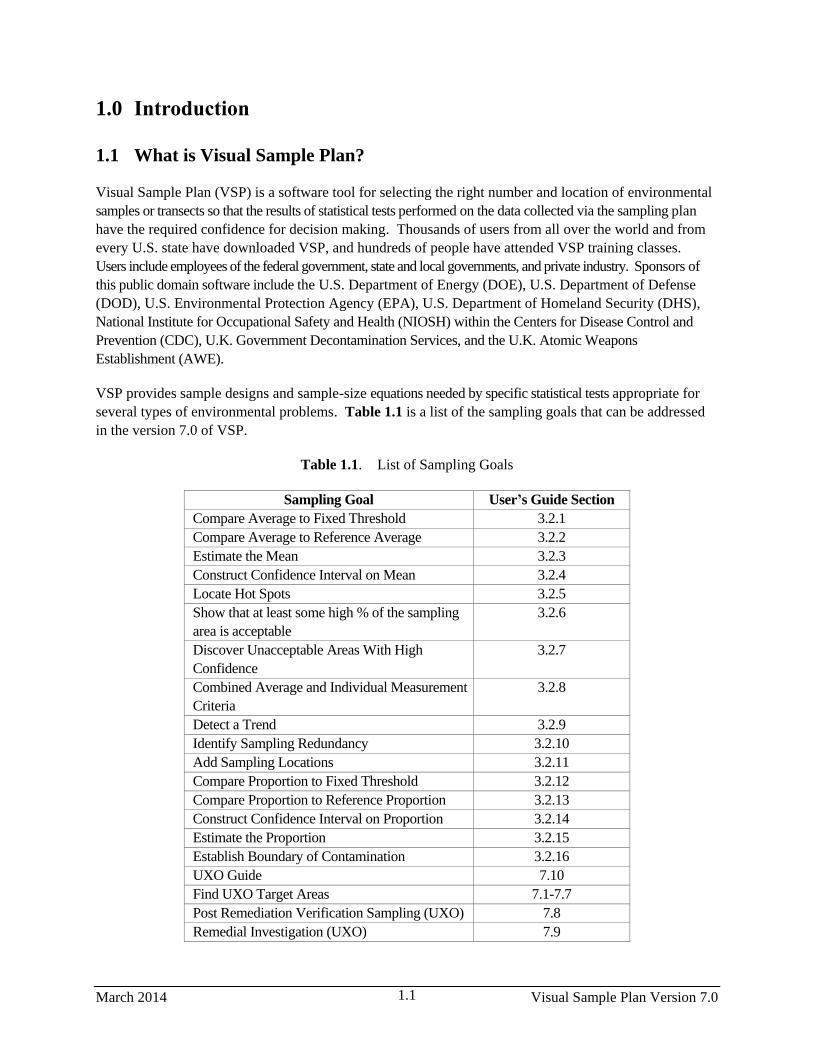
VSP provides sample designs and sample-size equations needed by specific statistical tests appropriate for
several types of environmental problems. Table 1.1 is a list of the sampling goals that can be addressed
in the version 7.0 of VSP.
Table 1.1. List of Sampling Goals
Sampling Goal User’s Guide Section
Compare Average to Fixed Threshold 3.2.1
Compare Average to Reference Average 3.2.2
Estimate the Mean 3.2.3
Construct Confidence Interval on Mean 3.2.4
Locate Hot Spots 3.2.5
Show that at least some high % of the sampling
area is acceptable
3.2.6
Discover Unacceptable Areas With High
Confidence
3.2.7
Combined Average and Individual Measurement
Criteria
3.2.8
Detect a Trend 3.2.9
Identify Sampling Redundancy 3.2.10
Add Sampling Locations 3.2.11
Compare Proportion to Fixed Threshold 3.2.12
Compare Proportion to Reference Proportion 3.2.13
Construct Confidence Interval on Proportion 3.2.14
Estimate the Proportion 3.2.15
Establish Boundary of Contamination 3.2.16
UXO Guide 7.10
Find UXO Target Areas 7.1-7.7
Post Remediation Verification Sampling (UXO) 7.8
Remedial Investigation (UXO) 7.9

Visual Sample Plan Version 7.0 March 2014 1.2
Sampling within a Building 3.2.21
Radiological Transect Surveying 3.2.22
Item Sampling 3.2.23
Non-statistical sampling approach 3.2.24
VSP is easy to use, highly visual, and graphical. It has extensive online help and tutorial guides. Reports
produced by VSP can be pasted directly into a quality assurance project plan, test plan, or sampling and
analysis plan. VSP can be used to implement EPA’s systematic planning process (EPA 2000a) for a
variety of problems: selection between clearly defined alternatives [Step 7 of the Data Quality Objectives
(DQO) process], studies where a confidence interval on an estimated parameter is needed, or determination of
whether a hot spot or target exists. The user specifies the criteria for “how good” the answer has to be
(Step 6 of the DQO Process), and VSP uses this as input to the formula for calculating the required
sample size. VSP is unique in this regard.
VSP is designed primarily for project managers and users who are not statistical experts, although those
individuals with statistical expertise also will find the software very useful.
1.2 Installation and System Requirements
VSP 7.0 runs on Microsoft Windows operating systems (Windows 8, Windows 7, Vista, and XP). VSP
currently does not run on Macintosh® or UNIX®/Linux systems. Any personal computer with sufficient
hardware to run one of the supported operating systems should run VSP. The minimum hardware
recommended is
1 GHz processor
256 MB RAM
250 MB of free space on the hard drive.
The current version of the VSP setup file is available from http://vsp.pnl.gov/ . After the setup file is
downloaded, installation of VSP is almost automatic. Simply run the VSP setup file, VSP70.exe (or later
version), and follow the on-screen instructions. The VSP program and auxiliary files will be copied by default
to the C:\Program Files\Visual Sample Plan folder (subdirectory). However, you may specify a different
location for the files.
Once installation is complete, you will start VSP using option Start > Program Files > Visual Sample
Plan > Visual Sample Plan. Alternatively, you may place a VSP shortcut on the desktop by selecting
New > Shortcut from the menu obtained by right-clicking the mouse on the desktop. The appropriate
command line for the default folder is
“C:\Program Files\Visual Sample Plan\VSample.exe”.
VSP may be uninstalled using the Control Panel icon labeled Add/Remove Programs. You may access
this option using the Start button and Control Panel.
New versions of VSP are often released as prototypes for testing. These demonstration versions have
expiration dates. After the expiration date has passed, you will be given the option of continuing with the

March 2014 Visual Sample Plan Version 7.0 1.3
current version or going to the VSP website to download the latest version. Version 7.0 is not a
demonstration version and does not have an expiration date.
1.3 Overview of VSP
Sampling is the process of gaining information about a population from a portion of that population
called a sample. A key goal of sampling design is to specify the sample size (number of samples) and
sampling locations that will provide reliable information for a specific objective (called the Sampling Goal)
at the least cost. VSP does the required calculations for sample size and sample location and outputs a
sampling design that can be displayed in multiple formats. VSP does not address sample collection
methods. It assumes the sample support (amount of material in the sample) is sufficient and the sample is
representative of the population. A few designs in VSP assume the sample is taken across an entire grid
(say a 10 x 10 cm swipe), but most designs assume the sample is a point sample taken at an X,Y
coordinate location, and has sufficient volume for measurement and testing. For appropriate sampling
goals, VSP addresses the trade-off between repeated analytical measurements on a single sample to reduce
overall sample result variability (measurement quality objectives / MQOs) and provides a sensitivity table
for comparing analytical methods of varying accuracy and cost.
VSP can be used to develop a new sampling design. It can also be used to compare alternative designs.
VSP automates the mechanical details of calculating sample size, specifying random sampling locations, and
comparing sample costs with decision error rates. These activities can be accomplished in the context of your
own site map displayed onscreen with various sampling plans overlain on sample areas that you select.
The first thing you will do after opening the program is to import or construct a visual map of the study
site. Next, you select the area or areas to be sampled. The Sample Area may be only a portion of the
study site (see the elliptical sample area in Figure 1.1, upper left window).
Then, for the Sampling Goal that you select, VSP will lead you through the quantitative steps of the DQO
process (Steps 6 and 7, EPA 2000a)) so that the program has the information needed to compute the
recommended minimum number of samples (sample size). You can enter sampling costs and test alternative
designs against a fixed budget.
The locations of the samples over the Sample Area are determined by the specific sampling design
(pattern) that you select. For some Sampling Goals, and for some assumptions about the population, only
certain designs are allowed from a statistical theory perspective. For example, sequential sampling is
appropriate only for the sampling goal of Compare Average to a Fixed Threshold when the population units
can be assumed to be distributed normally. When there is a choice of designs, VSP displays a selector for the
allowable designs.
VSP can be used for designing samples for environmental settings as well as building/room/surface
settings. For environmental settings, site maps and aerial pictures can be loaded into VSP for sample
placement. For buildings and rooms, a CAD drawing or floor plan are loaded. Map View displays
samples placed on maps and room drawings. On a site map, VSP displays the sample locations for easy
visualization (see Figure 1.1, upper left window). VSP also lists the geographical coordinates of the
sample locations (see Figure 1.1, lower right corner), which can be saved and exported as a Drawing
Exchange Format (DXF) or SHP file for use in a geographical information system (GIS) or saved as a text
file for use in global positioning system (GPS) software.

Visual Sample Plan Version 7.0 March 2014 1.4
Figure 1.1. Screen Capture from VSP Using Quad Window Option (Window > Quad Window)

March 2014 Visual Sample Plan Version 7.0 1.5
Several additional output formats for the design created in VSP are available: a Graph View of the
design (see Figure 1.1, upper right window), a Report View (see Figure 1.1, lower left window), a
Room View, and a 3D view. The Graph View displays either a Decision Performance Goal Diagram for
Sampling Goals that involved selecting between alternative actions, or a performance graph comparing
number of samples to a design parameter for the other classes of sampling goals. Some designs do not
have a Graph View. The Report View is a text report that describes the sampling design in detail. The
report contains the input values, the assumptions, the cost of the design, VSP output, technical description of
the sample size formula and algorithms used, and a sensitivity analysis table to assess what would happen
if more or fewer samples are collected than the optimal number calculated by VSP. The Room View
provides a variety of ways for viewing the surfaces in a room, while the 3D View allows for viewing
entire buildings or 3D areas.
The analytical value of lab results for samples can be input into VSP for Data Analysis including
summary statistics of results, statistical tests applied to results for making decisions, and graphical
displays of results. One of the designs, Sequential Sampling, requires intermediate results to be input to
VSP so that VSP can determine whether further sample collection is required.
1.4 How Do I Use VSP to Provide a Defensible Sampling Plan?
To defend a sampling plan to a regulator concerned about safety and to a citizens’ group concerned about
saving taxpayer dollars requires balancing cost and risk. Defensible means that sufficient samples are
taken, in a non-biased way, in order to make a decision, estimate a proportion, or declare an area free of
UXO/contamination with a stated level of confidence. Additionally, once samples are taken and the results
processed, someone needs to apply a statistical test to actually make a decision based on the data or
calculate a confidence interval. VSP incorporates all this into the code it uses to calculate a sample size
and sample locations. It asks the user to enter the assumptions, acceptable risk, and costs it needs for
these calculations.
VSP follows the EPA-sanctioned planning approach for data collection and decision-making called the Data
Quality Objectives (DQO) process. The DQO process achieves the user’s limit on acceptable risk, at a
minimum cost. See EPA (2000a) for an extended discussion of the DQO process. There are 7 steps in
the DQO process. Users must complete Steps 1 through 6 in order to have the inputs VSP needs. Then,
using VSP, the user can complete Step 7, “Optimize the Design for Obtaining Data,” because VSP can be
used to try out different sampling designs and find the optimal design for the current problem.
Users familiar with the DQO process know that often a single site may have multiple sampling goals and
multiple Sample Areas, each requiring its own set of DQO inputs and hence different sample require-
ments. VSP can help because it allows rapid prototyping and has many features that allow the overlay of
designs and comparisons across designs.
1.5 What’s New in VSP 7.0?
VSP 7.0 is a major new release of the software. Features new since version 6.0 include:
Non-UXO Sampling Designs
Design dialogs were improved to use sentence structure and blank defaults:

Visual Sample Plan Version 7.0 March 2014 1.6
- Parametric and Non-Parametric Upper Tolerance Limit (UTL)
- Adaptive Cluster
- Confidence interval on a mean (ordinary, MI sampling and non-parametric)
- Hot spot (assuming no false negative and assuming false negatives)
- Compare proportion to a fixed threshold
- Compare proportion to a reference proportion
New sample placement options to support 3D elevation surfaces
New non-geostatistical spatial mapping tools
Added default data columns for Control Chart design
Made improvements to list handling in Control Chart design
Lower / Upper Bound of the Gray Region won’t be affected when changing Action Level
Improvements to Kriging design dialog
Modified Collaborative designs to have blank default inputs
Changed Trend designs to use sentence structure
Improved graph and report views for I-Chart design
Updated I-Chart design to include “All Locations” selection
Added Contour sampling design for cases where having samples along contours is needed
Added Multiple increment hot spot sampling design
Added Discovery sampling design
UXO Sampling Designs
UXO 100% transect coverage analysis (for entire coverage of sample area and for 100% areas within
larger sample areas)
UXO design to augment existing paths with new transects
UXO Presumptively clean design

March 2014 Visual Sample Plan Version 7.0 1.7
Remedial Investigation design
TOI Rate design
Made various formatting changes to UXO Transect Spacing design dialog
Made improvements to Window Sizing option on locate and mark UXO design
Made improvements to UXO verification sampling, such as no default value for transect length and grid
size, random start for first transect
Made improvements to speed up UXO geostat functions
Added ability to see windowed densities used for UXO geostats
Added scaling option to UXO geostats to allow kriging to complete where it previously failed on high
densities
Added waypoint display for transects
Added ability to load text-based Recon data
Added Area Labels to Box Plots
Increased UXO Graph generation speed by using multiple processors
Added ability to pick a different point on Graph without re-running
Added import function to High Density Areas dialog page
Fixed UXO Transect Augmentation design dialog so that “Select All” COG updates properly
Made optimization improvements to Find Gaps in UXO Transect Augmentation design
Made improvements to Transect creation in UXO Transect Augmentation design
Made optimization improvements to Anomaly file import
Added option of keeping or removing transects when importing 100% Survey Areas
Added Target area definition options based on munition characteristics
Fixed storage and display of lag distance and lag tolerance for UXO Geostatistical analyses
“Save Graph” works from UXO Spacing page, even if Apply is not pressed
Made improvements to “Help me choose” Window Size dialog
Made improvements to UXO Transect Power Curve Graphs

Visual Sample Plan Version 7.0 March 2014 1.8
Fixed UXO Transect design to correctly calculate significant number of anomalies
Miscellaneous
Unaligned Grid Sample placement added for most designs that previously had the choice between random
and systematic grid sampling
Added dynamic sample groupings
Added ability to filter imported data based on built-in and user-defined parameters
Improvements to Analyte Page including user defined columns
Ability to import kriged data
Ability to move samples in rooms to specified surface or furniture
Improvements to samples on furniture
Improvements to show costs for actual number of samples on reports
Improvements to Furniture editor tool
Improvements to drawing guide spacing
Improvements to selection of Furniture, Surface Overlays and Room Labels
Improvements to Color Legends
Added ability to automatically create user-defined sample parameters during data import
Added plots to Mann-Kendall report when accounting for non-detects
Added room transparency in 3D view
Improved background image storage compression
Stair and Landing Editor
Four corner method for Google Earth image calibration
Floors in 3D view can be transparent
Displayed vertical faces for raised surface overlays
Added storage compression for image data
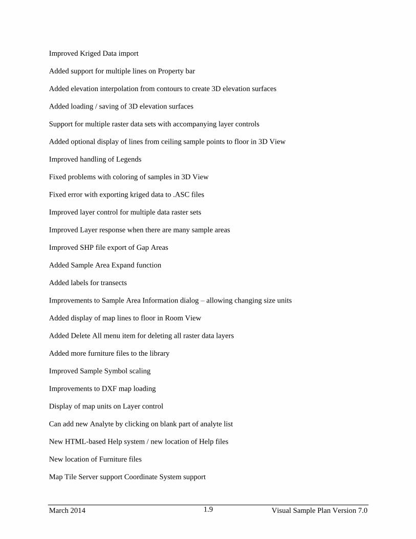
March 2014 Visual Sample Plan Version 7.0 1.9
Improved Kriged Data import
Added support for multiple lines on Property bar
Added elevation interpolation from contours to create 3D elevation surfaces
Added loading / saving of 3D elevation surfaces
Support for multiple raster data sets with accompanying layer controls
Added optional display of lines from ceiling sample points to floor in 3D View
Improved handling of Legends
Fixed problems with coloring of samples in 3D View
Fixed error with exporting kriged data to .ASC files
Improved layer control for multiple data raster sets
Improved Layer response when there are many sample areas
Improved SHP file export of Gap Areas
Added Sample Area Expand function
Added labels for transects
Improvements to Sample Area Information dialog – allowing changing size units
Added display of map lines to floor in Room View
Added Delete All menu item for deleting all raster data layers
Added more furniture files to the library
Improved Sample Symbol scaling
Improvements to DXF map loading
Display of map units on Layer control
Can add new Analyte by clicking on blank part of analyte list
New HTML-based Help system / new location of Help files
New location of Furniture files
Map Tile Server support Coordinate System support

Visual Sample Plan Version 7.0 March 2014 1.10
File Save As previous VSP version
RAMS Import/Export
Building Footprints on wide area map
Allow manual moving of samples
Ft/Inch display options on map and coordinate view
UXO Guide
Sampling Height for rooms
Find Targets / UXO Geostat Mapping can select subset of transects for analysis
Crisis Management Mentor
Scale Map to Background Image
Ability to include/exclude 100% grid areas in GAMV & KT3D calculations
Outlier marking for data grid differences
Contour Sampling design Report / Help
Automatic removal of duplicate transects and anomalies
Added display of furniture to map view
New OLE Automation functions
Show Grid Cell Corner Coordinates

March 2014 Visual Sample Plan Version 7.0 2.1
2.0 Mechanics of Running VSP
2.1 Getting Started and Navigational Aids
Upon launching VSP, the first screen you will see is “Welcome to Visual Sample Plan” overlain with the
initial navigational screen, “Select VSP Version” (Figure 2.1).
Figure 2.1. VSP Welcome Screen with Version Selection Menu
The choice of VSP versions is offered because different versions of VSP have been developed for
different sponsors. Versions were designed to simplify the options presented to the single-purpose user as
VSP became more complex. For example, the UXO Detection Application Version implements only
those sampling designs used for sites which may contain UXO. Users interested only in MARSSIM
applications can select the MARSSIM Application Version. That version contains menu items relating
to only rooms and surfaces, and its statistical tests and sampling design options are limited to only those
that are MARSSIM-approved. Users only interested in RCRA applications can select the RCRA
Version, which focuses on designs for monitoring and trends. The CDC/NIOSH version contains menu
items related to rooms, surfaces, and statistical testing and analysis related to that kind of sampling. The
FRMAC CM version launches an expert guide that points the user to information about the next module
they will be using. The General (all inclusive) VSP version provides access to all sampling designs and
options.
Having selected a VSP version, you are now at the “Welcome to Visual Sample Plan” screen. The
instructions on this page give answers to the most commonly asked questions from new VSP users. This
screen will stay up until it is overlain with one of the View options. For example, when a map is loaded
and you are in Map View.

Visual Sample Plan Version 7.0 March 2014 2.2
You now are ready to begin using VSP. The main toolbar buttons (select View > Main Toolbar to see
the buttons) offer a quick, one-click method for performing the primary VSP functions. The pull-down
menus offer a wider range of options. Pull-down menus and buttons are shown in Figure 2.2. Holding
the mouse over a button will reveal in text what that button does. For example, the Undo button is for
undoing a key stroke during a map drawing session.
Figure 2.2. Main Menu Items (top row) and Buttons on the Toolbar (bottom row)
There are 4 separate toolbars: the main toolbar, map drawing toolbar, ranked set toolbar, and room
toolbar. These toolbars can be moved around the screen by placing the mouse above the buttons on the
toolbar and dragging to another place. Toolbars can be displayed or hidden depending on whether they
are checked or not (see View pulldown list).
Starting with the File menu item on the top menu bar, the pull-down menu shows the various options for
dealing with Projects.
VSP uses the term “Project” to refer to the map, report, sample information, and cost information
associated with one sampling design. All this information is contained in the ‘filename.VSP’ file created
or selected by the user and is in a special VSP format. Upon starting VSP, you either create a new
project, File > New Project, or open an existing project, File > Open Project (Figure 2.3). If you are
creating a new project, you will automatically be put into the “Welcome to Visual Sample Plan” screen
after selecting File > New Project. If you are opening an existing project, you will be shown a list of
existing VSP files and asked to browse and select one.
2.2 Setting Up a Map
If you are starting a new project, you may obtain a map
(drawing) of the site in any of three ways:
1. Import the site map from a drawing interchange format
(DXF) file or ArcView SHP file, or import a Geosoft or
RAMS project. VSP supports the following DXF
Objects: POLYLINE, LWPOLYLINE, LINE, ARC,
CIRCLE, ELLIPSE, TEXT. If you are having problems
loading a DXF file into VSP, try converting your file to
these types of objects.
2. Import the site map from a previous VSP project that
was saved in VSP format (i.e., a .VSP file).
3. Draw the map or Sample Area using VSP’s drawing
tools.
These three methods are illustrated below. VSP uses the coordinate system associated with the imported
map. Because neither DXF nor SHP files contain the distance units, VSP will assume your map is in feet
until you change it to some other unit. This is done by selecting Map > Map Settings from the Main
Menu. If you want to use a local origin in your design, use Map > Set Origin to click on the map at the
Figure 2.3. Pull-Down Menu
Items Under File

March 2014 Visual Sample Plan Version 7.0 2.3
location you want to become the new origin (0,0 point). You can also input the current location via the
keyboard to become the new origin. If the SHP map is in Latitude / Longitude, rather than a planar
coordinate system, VSP will recognize it and offer to convert it to the Universal Transverse Mercator
(UTM) system.
2.2.1 Importing a Site Map from a File
You can draw a complex site map in an architectural drawing program such as Autodesk
Map, AutoCAD, or ArcView and save the drawing to a .DXF or SHP formatted file in that software
package. The resulting file can be imported into VSP. You can also import a Geosoft project which
contains a map. The Millsite.dxf file is a sample DXF file provided with VSP. The following steps
illustrate how to use this file in VSP:
1. From the main menu, select Map > Load Map from File. A quick alternative is to click on the
Load Map button on the VSP toolbar.
2. A list of available files in the Visual Sample Plan folder is displayed. Select Millsite.dxf. You may
change folder names to search for the desired file using standard Microsoft file-searching if the file
is not in the Visual Sample Plan folder. Double-click on Millsite.dxf.
3. Select which layers you want to import from the map file.
4. Choose whether or not you want to import the text embedded in the DXF file.
The site map should appear on your screen as illustrated in Figure 2.4. SHP files loaded in the same
manner. Geosoft and RAMS project files are imported by selecting File > Import > from Geosoft /
from RAMS.
Figure 2.4. The Millsite.dxf File Opened in VSP, showing MAP Pull-down Menu

Visual Sample Plan Version 7.0 March 2014 2.4
2.2.2 Importing a Site Map File in the VSP Format
To open a VSP-formatted file, from the main menu select File > Open Project or use the Open button on
the VSP toolbar. A list of available VSP files is displayed. Double click on the .VSP file to be opened.
Switch folders and/or directories if the desired file is in another folder or directory.
2.2.3 Draw Map Using VSP Drawing Tools
VSP provides a basic set of drawing tools for users who do not have a drawing program to create a site
map. You can experiment with the drawing tools as follows:
Create a new project by choosing File > New Project on the Main Menu or by clicking the New
button on the main toolbar. To dismiss the “Welcome to Visual Sample Plan” displayed upon
opening a new project, simply commence one of the drawing operations outlined below or an
operation in Map > Map Settings. If the project window is not full screen, expand the project
window by pressing the Maximize button on the upper right corner of the project window.
Choose View > Map Drawing Toolbar from the Main Menu. This displays a toolbar used
specifically for drawing a map. This toolbar also may be docked if you prefer to move it from the
project window. To dock the drawing toolbar, place the mouse cursor on the blue title bar and drag
the drawing toolbar onto the VSP toolbar.
All the drawing functions described below also are available from the Main Menu option Map.
Draw Line. Click the Draw Line button on the toolbar, or select Map > Draw Line or Polyline. The
cursor will become a cross, indicating that you are in drawing mode. Click a point on the map. You will
now see a line between the cursor and point you clicked. Continue clicking points to make a complex
polygon. If you make a mistake, click the Undo button on the VSP toolbar (or select Edit > Undo from
the Main Menu or press Ctrl-Z on the keyboard). This will remove the last point you entered.
Points can also be entered on the keyboard. Just enter the x, y coordinates for each point (for example:
type 32,48 and press the Enter key). You can see the coordinates that you are entering on the status bar at
the bottom of the window. To connect a line to a point already entered (for example, to connect the last
line to the first point to create a closed polygon), hold the Shift key while clicking with the mouse.
Holding the Shift key can be used in most drawing operations to select the nearest point on the map
without having to carefully position the cursor. Holding the Ctrl key while moving the mouse allows you
to draw a horizontal or vertical line without having to be careful. To finish the line, right-click the mouse
or click the Draw Line button on the toolbar again.
Draw Rectangle. Click the Draw Rectangle button on the toolbar, or select Map > Draw Rectangle.
Click on a point on the map that you want to be one corner of a rectangle. Holding the Shift key while
clicking causes that point to be attached to an existing point on the map. Move the cursor to the opposite
corner of the rectangle and click the mouse button. Holding the Ctrl key while moving and clicking
forces the rectangle to be a square. The x, y coordinates of the corner points can be entered on the
keyboard also. A rectangle of a specific size can be defined by typing the dimensions (for example: type
200x100 and press the Enter key). You can see the dimensions that you are entering on the status bar at
the bottom of the window. The rectangle of the specified size will be created with its lower left corner at
the coordinate 0,0.

March 2014 Visual Sample Plan Version 7.0 2.5
Draw Ellipse. Click the Draw Ellipse button
on the toolbar, or select Map > Draw Ellipse.
Drawing an ellipse is basically the same as
drawing a rectangle. Holding the Ctrl key
forces the ellipse to be a circle.
Draw Curve. Click the Draw Curve button
on the toolbar, or select Map > Draw Curve.
Click a point on the map. Click a second point
on the map. A line is drawn between these
first two points. As you move the cursor
around the map, this line is stretched to
become a curve. When the curve has the
shape you want, click the mouse (this is the
control point). The x, y coordinates for the
three points also can be entered on the
keyboard.
Add Annotation. Notes (also called note
objects) can be added to maps using the
annotation tool. Select Map > Add
Annotation, and the cursor becomes a
crosshair. Click on the map at the location
where you want to add the note object. The
location may also be entered on the keyboard. A default object containing the text “Right-Click Here” is
added to the map.
After the default object is added, use the mouse to right-click on the note object. A Map Label
Information dialog box pops up, as shown in Figure 2.5. You will be able to change the following
parameters:
Note text
Anchor point on map
Anchor point to screen
X and Y coordinates of anchor point (map or screen)
Border, background color, and font
Alignment (left/center/right, top/center/bottom)
Show Drawing Guide. Selecting Map > Show Drawing Guide turns the Snap-To Drawing Guide on or
off. This guide works with most of the drawing functions, causing the shape you draw to be exactly
aligned to a grid. When you turn on the Drawing Guide, a dialog is shown that allows you to specify the
spacing of the grid and the color of the points shown on the screen.
2.2.4 Working with Maps
2.2.4.1 Selecting Lines and Notes on the Map
VSP imports DXF and SHP files and turns the objects into polylines or a series of connected points.
Lines and note objects on the map can be selected by clicking on them with the mouse. When an object is
Figure 2.5. Map Label Information Dialog Box

Visual Sample Plan Version 7.0 March 2014 2.6
selected, a small black box appears at each vertex, or point, on the object. Polylines appear as a series of
vertices. Hold the Ctrl key down while clicking to toggle the selected status of a single line or note
(annotation) object.
Several lines may be selected by using a rectangular area. To do this, position the mouse at one corner of
the rectangle then press and hold the left mouse button down while moving the mouse to the opposite
corner of the rectangle. When the mouse button is released, all the lines and notes that pass through the
rectangle will be selected. Use the Ctrl key to keep previously selected lines and note objects.
Move Selected Objects. Use this dialog by selecting Map > Move Selected Objects to move the
selected objects by the given offsets. Objects may also be moved by using the mouse. Position the
mouse over a selected line or note object. Press and hold the left mouse button while moving the mouse
to the new position. When the mouse button is released, the selected lines will be placed at the new
position. This command applies to both map lines and note objects.
Rotate Selected Objects. After selecting Map > Rotate Selected Objects, enter the pivot point by
clicking with the mouse or entering the coordinates on the keyboard. Then enter the angle of rotation by
moving the mouse and clicking or entering the degrees on the keyboard. This command affects all
selected objects on the map.
Delete Selected Objects. This command deletes selected objects from the map (Map > Delete Selected
Objects). This action cannot be undone.
Insert Point. After selecting Map > Insert Point, click on the map with the mouse. A new vertex point
is inserted in the nearest polyline on the map. If the polyline matches a sample area, then a matching
vertex is also inserted into the sample area. An individual point can be selected by holding the Shift key
while clicking on the point, allowing it to be dragged to a new location. Holding the control key will
keep the point aligned vertically or horizontally. Selecting a segment is done in much the same way by
holding the Shift key while clicking on a segment between two points, dragging it, and holding the Ctrl
key to keep alignment vertical or horizontal.
Deleting Segments of a Map. If you want to remove a segment from either an imported map or a user-
drawn map, you may click on a segment and hit the Delete key on your keyboard. Left-clicking on any
segment in a map displays the vertices of the polyline in an outline of bold squares. With the outline in
bold squares displayed, hit the Delete key on your keyboard and that segment is removed.
Map Buttons on the Toolbar. The Zoom In, Zoom Out, Zoom Window, Zoom Max, and Pan buttons
in the middle of the VSP toolbar (and as pulldown items under Main Menu option View) provide methods
to focus in on a Sample Area or other region of a site map. Press once on the Zoom In button and then
click on the site map to make it grow larger. Turn off this mode by pressing the Zoom In button again.
The Zoom Out button works the same way except that it makes the site map shrink. The location on the
site map where you click determines the area of the new focus.
The Zoom Window button allows you to create an expanded rectangular window into the site map. For
an example, press the Zoom Window button, drag the cursor across part of the screen, and release. The
dashed lines illustrate the final window focus.

March 2014 Visual Sample Plan Version 7.0 2.7
The Zoom Max button displays the map at the largest size that will fit the current view. VSP uses the
current map extents to determine how the map will be positioned. Use Map > Map Settings to adjust the
minimum / maximum x and y coordinates to use for this operation.
The Pan button repositions the map in the view window. Hold the left mouse button while dragging the
map to a new location. When the left mouse button is released, the map will be redrawn at the new
position.
2.2.5 Additional Map Features
The remaining pull-down menu items under MAP are specialty topics, some of which are discussed in
other sections of this manual. They will be briefly defined here.
Sample Points imports and exports sample points to text files. It is discussed in Section 2.5. Export
Map exports a map and/or samples to various file formats. Draw Transects allows you to manually
create transects on the map. To draw transects on the map you must first enter the width of the transects
in the dialog that appears. Transects will only be added inside of existing sample areas. If you draw
outside sample areas, the transects will be clipped at the edge of the sample areas. This command works
similar to the Draw Line command. Right-click with the mouse or re-select this command to stop
drawing. This command is useful for creating transects to be analyzed with Sampling Goals > Find
Target Areas and Analyze Survey Results (UXO) > Assess probability of target area traversal
based on actual transect pattern.
Map > Background Picture > Load from file loads a background picture from a graphics file into VSP.
VSP comes with two sample pictures: VSPEx1 and VSPEx2. Once a picture file is loaded into VSP,
sample areas can be located on the picture similar to how they are located on a map. Coordinate System
allows you to tell VSP which Projected Coordinate System (PCS) the project map is in. If you have
loaded your map from a SHP file with and associated PRJ file, VSP will automatically set the coordinate
system from the PRJ file.
Map > Background Picture > Calibrate Picture to Map matches the background picture to the
sampling map. Map > Background Picture > Calibrate Google Earth Image allows you to use an
image obtained from Google Earth and calibrate it to the VSP sampling map. Map > Background
Picture > Load World File can be used if a Picture World File is available for the background picture.
Map > Background Picture > Scale Map to Background allows you to scale the current map so that
map distances match the distances represented in the background picture. Map > Background Picture >
Save World File takes a background picture that has been calibrated either through loading a world file
or by manually calibrating the picture, and writes a world file to save the picture calibration information.
Figure 2.6 shows the background picture VSPEx1 loaded into VSP with a yellow sample area labeled
“Sample area 1” placed on the picture. Map > Background Picture > Connect to Tile Server allows
you to automatically show a background image map from an image tile server. In order to use this
feature, you must first set your coordinate system from the Map menu, so the VSP knows how to align the
images with your project map. The tile server background image can also be enabled from the Layer
Control under Background Images.

Visual Sample Plan Version 7.0 March 2014 2.8
Create Lines for Areas creates
outlines around sample areas that
don’t currently have them. These
outlines are important, because they
allow you to edit the size and shape
of a sample area.
Crop Map removes portions of a
map that are not currently visible
on the view window. It is useful
for removing large amounts of
extraneous map lines that tend to
slow down the display and other
map functions.
Kriged or Other Raster Data
contains options for importing and
exporting raster-type data, such as
Kriged results. Imported files use
the ESRI grid format to allow it to
be read into ArcGIS or other
programs supporting the grid file
format.
Elevation Data contains options
for importing and exporting
information on surface elevations
for sample areas, with data being stored in an ESRI grid file.
UXO Recon Data contains an option for importing UXO reconnaissance data from a text file.
Import CONTAM Data contains an option for importing data from the CONTAM software.
Insert Building Footprint allows you to place a representation of building rooms from another VSP
project file onto the current project map.
Refer to Section 6.1.3 for a discussion of using CAD drawings of building floor plans to delineate
rooms/sampling areas within the floor plan drawings.
2.3 Sample Areas in VSP
2.3.1 Creating a Sample Area
Once a map is created, a Sample Area must be created. A Sample Area is a region in which to locate
samples. While most sample areas are enclosed, one of the Sampling Goals in VSP, Establish Boundary
of Contamination, allows for an open type of sample area -- samples are located along a boundary. The
user must identify the area to VSP in order to make sampling locations available. (Note: Sampling
Figure 2.6. Background Picture (.jpeg image) Loaded into VSP
as a Map, with Labels Added
Label Added
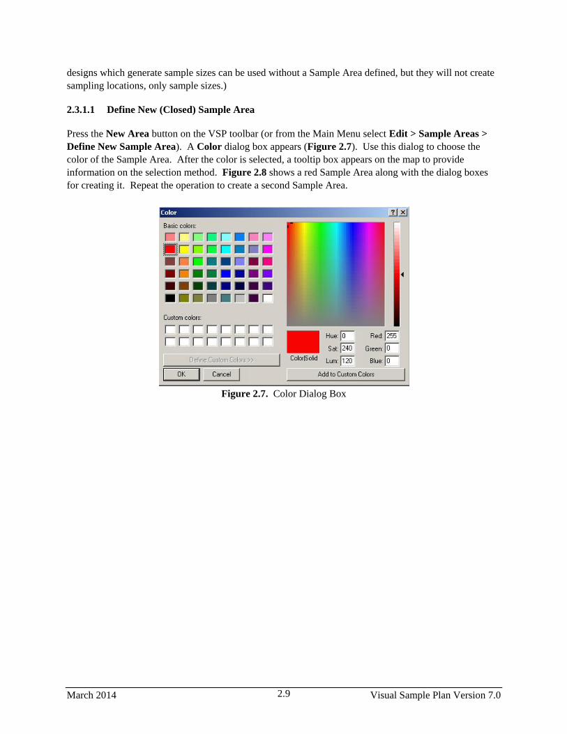
March 2014 Visual Sample Plan Version 7.0 2.9
designs which generate sample sizes can be used without a Sample Area defined, but they will not create
sampling locations, only sample sizes.)
2.3.1.1 Define New (Closed) Sample Area
Press the New Area button on the VSP toolbar (or from the Main Menu select Edit > Sample Areas >
Define New Sample Area). A Color dialog box appears (Figure 2.7). Use this dialog to choose the
color of the Sample Area. After the color is selected, a tooltip box appears on the map to provide
information on the selection method. Figure 2.8 shows a red Sample Area along with the dialog boxes
for creating it. Repeat the operation to create a second Sample Area.
Figure 2.7. Color Dialog Box

Visual Sample Plan Version 7.0 March 2014 2.10
Figure 2.8. Define New Sample Area
There are two basic ways in which to create the Sample Area:
1. One-Step Method. Position the cursor inside one of the enclosed areas on the map and right-click
with the mouse. The Sample Area is created, and a dialog box appears. This dialog box shows the
size of the Sample Area. Click the OK button on the dialog when done.
2. Corner-Selection Method. Position the cursor on each corner of the Sample Area and left-click
with the mouse. If you hold down the Shift key while clicking, the nearest point on the map will be
selected. If you make a mistake in choosing a corner, use the
Undo feature. When you have finished defining the Sample
Area, either click the Finish Area button on the VSP toolbar,
select Main Menu option Edit > Sample Areas > Finish
New Sample Area, or right-click the last segment in the
corner selection method. The area dialog box appears
(Figure 2.9). Note: A Sample Area cannot cross over itself.
If this happens, an error message—”This area is not valid
and will be removed”—appears.
Figure 2.9. Map with a Single
Sample Area
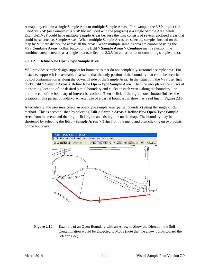
March 2014 Visual Sample Plan Version 7.0 2.11
A map may contain a single Sample Area or multiple Sample Areas. For example, the VSP project file
OneAcre.VSP (an example of a VSP file included with the program) is a single Sample Area, while
Example1.VSP could have multiple Sample Areas because the map consists of several enclosed areas that
could be selected as Sample Areas. When multiple Sample Areas are selected, samples located on the
map by VSP are distributed across all the areas. When multiple samples area are combined using the
VSP Combine Areas toolbar button or the Edit > Sample Areas > Combine menu selection, the
combined area is treated as a single area (see Section 2.3.5 for a discussion of combining sample areas).
2.3.1.2 Define New Open-Type Sample Area
VSP provides sample design support for boundaries that do not completely surround a sample area. For
instance, suppose it is reasonable to assume that the only portion of the boundary that could be breached
by soil contamination is along the downhill side of the Sample Area. In that situation, the VSP user first
clicks Edit > Sample Areas > Define New Open-Type Sample Area. Then the user places the cursor at
the starting location of the desired partial boundary and clicks on each vertex along the boundary line
until the end of the boundary of interest is reached. Then a click of the right mouse button finishes the
creation of this partial boundary. An example of a partial boundary is shown as a red line in Figure 2.10.
Alternatively, the user may create an open-type sample area (partial boundary) using the single-click
method. This is accomplished by selecting Edit > Sample Areas > Define New Open-Type Sample
Area from the menu and then right clicking on an existing line on the map. The boundary may be
shortened by selecting the Edit > Sample Areas > Trim from the menu and then clicking on two points
on the boundary.
Figure 2.10. Example of an Open Boundary with an Arrow to Show the Direction the Soil
Contamination would be Expected to Move (note that the arrow points toward the
“clean” side)
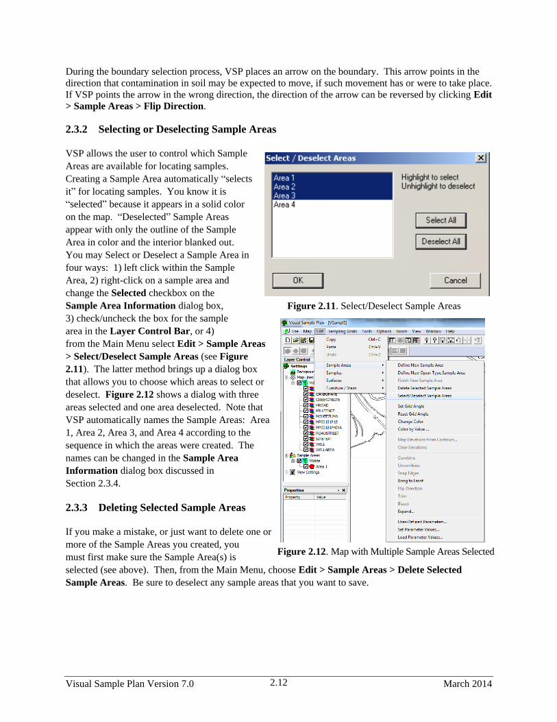
Visual Sample Plan Version 7.0 March 2014 2.12
During the boundary selection process, VSP places an arrow on the boundary. This arrow points in the
direction that contamination in soil may be expected to move, if such movement has or were to take place.
If VSP points the arrow in the wrong direction, the direction of the arrow can be reversed by clicking Edit
> Sample Areas > Flip Direction.
2.3.2 Selecting or Deselecting Sample Areas
VSP allows the user to control which Sample
Areas are available for locating samples.
Creating a Sample Area automatically “selects
it” for locating samples. You know it is
“selected” because it appears in a solid color
on the map. “Deselected” Sample Areas
appear with only the outline of the Sample
Area in color and the interior blanked out.
You may Select or Deselect a Sample Area in
four ways: 1) left click within the Sample
Area, 2) right-click on a sample area and
change the Selected checkbox on the
Sample Area Information dialog box,
3) check/uncheck the box for the sample
area in the Layer Control Bar, or 4)
from the Main Menu select Edit > Sample Areas
> Select/Deselect Sample Areas (see Figure
2.11). The latter method brings up a dialog box
that allows you to choose which areas to select or
deselect. Figure 2.12 shows a dialog with three
areas selected and one area deselected. Note that
VSP automatically names the Sample Areas: Area
1, Area 2, Area 3, and Area 4 according to the
sequence in which the areas were created. The
names can be changed in the Sample Area
Information dialog box discussed in
Section 2.3.4.
2.3.3 Deleting Selected Sample Areas
If you make a mistake, or just want to delete one or
more of the Sample Areas you created, you
must first make sure the Sample Area(s) is
selected (see above). Then, from the Main Menu, choose Edit > Sample Areas > Delete Selected
Sample Areas. Be sure to deselect any sample areas that you want to save.
Figure 2.12. Map with Multiple Sample Areas Selected
Figure 2.11. Select/Deselect Sample Areas
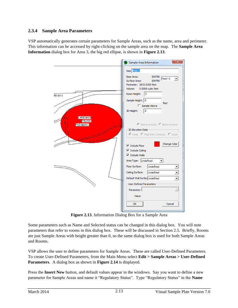
March 2014 Visual Sample Plan Version 7.0 2.13
2.3.4 Sample Area Parameters
VSP automatically generates certain parameters for Sample Areas, such as the name, area and perimeter.
This information can be accessed by right-clicking on the sample area on the map. The Sample Area
Information dialog box for Area 3, the big red ellipse, is shown in Figure 2.13.
Figure 2.13. Information Dialog Box for a Sample Area
Some parameters such as Name and Selected status can be changed in this dialog box. You will note
parameters that refer to rooms in this dialog box. These will be discussed in Section 2.5. Briefly, Rooms
are just Sample Areas with height greater than 0, so the same dialog box is used for both Sample Areas
and Rooms.
VSP allows the user to define parameters for Sample Areas. These are called User-Defined Parameters.
To create User-Defined Parameters, from the Main Menu select Edit > Sample Areas > User-Defined
Parameters. A dialog box as shown in Figure 2.14 is displayed.
Press the Insert New button, and default values appear in the windows. Say you want to define a new
parameter for Sample Areas and name it “Regulatory Status”. Type “Regulatory Status” in the Name

Visual Sample Plan Version 7.0 March 2014 2.14
box. Say you select “Integer” for Type, and check the List option. List lets you limit the values assigned
to Regulatory Status to those you supply. Figure 2.15 displays the dialog box for User Defined Area
Parameters.
With a parameter highlighted in the Select Parameter to
Modify window, hit the Edit List button. A new dialog box
titled Parameter List Values comes up (see Figure 2.16).
The user inputs values to this list by putting the mouse on a
current value, hitting return, and typing the next value into
the list. The list contains the valid arguments for that
parameter.
Once a new parameter is defined, that parameter is attached
to (or defined for) all Sample Areas. You may want some
Sample Areas to have one value for the parameter, and other
Sample Areas have another value. Parameter values may be
set in the Sample Area Information dialog or by the Edit >
Sample Areas > Set Parameter Values menu command.
Shown in Figure 2.17, the Set Parameters dialog box
allows the user to assign parameter values to Sample Areas
based on a condition. The example says to set the parameter Regulatory Status to the value “4” for
Sample Areas that have a Base Area (one of the VSP-defined Sample Area parameters) greater than or
equal to 100 square feet. The Set Parameters dialog box has many pull-down lists, making it easy for the
user to quickly set parameter values for Sample Areas.
Figure 2.14. User Defined Area Parameters
Dialog Box
Figure 2.16. Parameter List Values
Dialog Box
Figure 2.15. User Defined Area Parameters
Dialog Box with Edit List
Dialog Box with Edit List
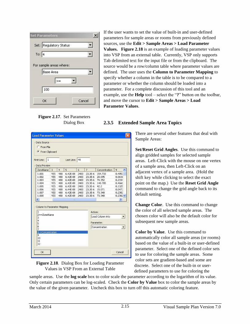
March 2014 Visual Sample Plan Version 7.0 2.15
If the user wants to set the value of built-in and user-defined
parameters for sample areas or rooms from previously defined
sources, use the Edit > Sample Areas > Load Parameter
Values. Figure 2.18 is an example of loading parameter values
into VSP from an external table. Currently, VSP only supports
Tab delimited text for the input file or from the clipboard. The
source would be a row/column table where parameter values are
defined. The user uses the Column to Parameter Mapping to
specify whether a column in the table is to be compared to a
parameter or whether the column should be loaded into a
parameter. For a complete discussion of this tool and an
example, use the Help tool – select the “?” button on the toolbar,
and move the cursor to Edit > Sample Areas > Load
Parameter Values.
2.3.5 Extended Sample Area Topics
There are several other features that deal with
Sample Areas:
Set/Reset Grid Angles. Use this command to
align gridded samples for selected sample
areas. Left-Click with the mouse on one vertex
of a sample area, then Left-Click on an
adjacent vertex of a sample area. (Hold the
shift key while clicking to select the exact
point on the map.) Use the Reset Grid Angle
command to change the grid angle back to its
default setting.
Change Color. Use this command to change
the color of all selected sample areas. The
chosen color will also be the default color for
subsequent new sample areas.
Color by Value. Use this command to
automatically color all sample areas (or rooms)
based on the value of a built-in or user-defined
parameter. Select one of the defined color sets
to use for coloring the sample areas. Some
color sets are gradient-based and some are
discrete. Select one of the built-in or user-
defined parameters to use for coloring the
sample areas. Use the log scale box to color scale the parameter according to the logarithm of its value.
Only certain parameters can be log-scaled. Check the Color by Value box to color the sample areas by
the value of the given parameter. Uncheck this box to turn off this automatic coloring feature.
Figure 2.17. Set Parameters
Dialog Box
Figure 2.18. Dialog Box for Loading Parameter
Values in VSP From an External Table

Visual Sample Plan Version 7.0 March 2014 2.16
Combine. This command combines sample areas or creates interior holes in sample areas. To combine
sample areas, select 2 or more non-overlapping sample areas on the map and use this command. The
sample areas are combined so that they are treated as a single sample area. Clicking on one part of the
sample area will select or deselect all the attached parts of the sample area. All the attached parts are
treated as a single sample area for the purpose of sample placement. See Help > Help Topics > Menus >
Edit menu > Sample Areas > Combine for an example. Use Uncombine to reverse the effect of the
Combine Sample Areas and breaks combined sample areas into the component areas.
Snap Edges. When edges and corners of adjacent sample areas to not exactly match up, use this
command to perfectly align them. The edges must be fairly close to each other, they may even overlap
slightly. After using this command, the edges will not overlap nor have any space between them.
Bring to Front. Use this command to bring the selected sample areas to the end of the draw list causing
them to be drawn last. This will, in effect, cause them to appear in front of other sample areas. Use this
command for sample areas that exist inside the hole of another sample area and cannot be seen. Note that
this command changes the sample area numbers.
Flip Direction. This command switches the contaminated /
uncontaminated side of the open-type sample area. The arrow
points toward the uncontaminated side.
Trim. This command allows you to shorten the open-type sample
area. After selecting this command, the cursor becomes a cross-
hair. Use the mouse to click on two points on the open-type area.
After the second point is selected, the area will be truncated at the
two points.
Bisect. Use this command to split a sample area into one or more
parts. To bisect: (1) Draw a line on the map that crosses the
sample area one or more times, (2) Select the line, (3) Choose this
command from the menu.
Expand. Use this command to expand all selected sample areas
outward by a specified distance.
Map Elevations from Contours. This command allows you to
create elevation mappings from contour lines in VSP.
Clear Elevations. This command removes elevation mappings
from all selected sample areas.
2.4 Map Layers and Properties in VSP
The Layer Control Bar (Figure 2.19) is displayed by selecting
View > Layer Bar. The Layer Control provides quick access to
turning on / off:
Figure 2.19. Layer Control Bar

March 2014 Visual Sample Plan Version 7.0 2.17
Map Lines
Samples Areas
View Settings
The power of the Layer Control lies in its ability to turn off multiple map lines or sample areas based on
different organizing criteria. Another powerful feature is that each View Window in VSP has
independent Layer settings – so each window can display different map lines, sample areas, etc.
2.4.1 Map Lines
The display of map lines can be turned on or off using the Layer
Control. By checking the box next to the name of the map, all the lines
for the map can be toggled. In Figure 2.20, there are two maps: Base
and Football.
If the map that was loaded is a DXF file, it may contain more than one
Layer. If so, the lines for individual layers can be toggled by checking
the box next to the names of the individual layers. In Figure 2.20, the
Base map contains layers named 0, BLDG, CREEK, etc. and the
Football map contains layers named
BOUNDARY, ENDZONE, etc.
2.4.2 Sample Areas
Individual sample areas can be turned on or off by
checking the box next to the name of the sample
area. If the VSP project contains multiple maps,
all the sample areas associated with a map can be
toggled by checking the name of the map under the
Sample Areas category. In Figure 2.21, there are
two maps (which are two floors in a building):
ccbasement and ccmainfloor. By checking the box
next to ccbasement, all the sample areas associated
with the map ccbasement will be toggled on or off.
This makes it easy to work with the floors of the
building individually - if desired. In addition,
because each View Window has independent layer
settings, one window can view the basement and
another window can view the main floor.
When user-defined sample area parameters exist,
VSP can toggle sets of sample areas bases on those
parameters. In Figure 2.22, there are 3 parameters
that can be used to toggle sample areas: Zone,
Release and Class. By checking or unchecking the
Figure 2.20. Map Lines
Figure 2.22. Sample
Areas
Figure 2.21. User-
Defined Parameters
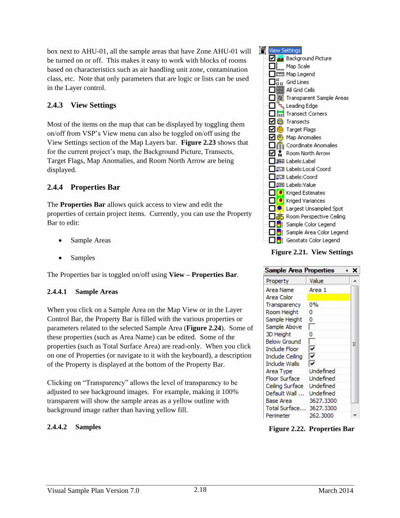
Visual Sample Plan Version 7.0 March 2014 2.18
box next to AHU-01, all the sample areas that have Zone AHU-01 will
be turned on or off. This makes it easy to work with blocks of rooms
based on characteristics such as air handling unit zone, contamination
class, etc. Note that only parameters that are logic or lists can be used
in the Layer control.
2.4.3 View Settings
Most of the items on the map that can be displayed by toggling them
on/off from VSP’s View menu can also be toggled on/off using the
View Settings section of the Map Layers bar. Figure 2.23 shows that
for the current project’s map, the Background Picture, Transects,
Target Flags, Map Anomalies, and Room North Arrow are being
displayed.
2.4.4 Properties Bar
The Properties Bar allows quick access to view and edit the
properties of certain project items. Currently, you can use the Property
Bar to edit:
Sample Areas
Samples
The Properties bar is toggled on/off using View – Properties Bar.
2.4.4.1 Sample Areas
When you click on a Sample Area on the Map View or in the Layer
Control Bar, the Property Bar is filled with the various properties or
parameters related to the selected Sample Area (Figure 2.24). Some of
these properties (such as Area Name) can be edited. Some of the
properties (such as Total Surface Area) are read-only. When you click
on one of Properties (or navigate to it with the keyboard), a description
of the Property is displayed at the bottom of the Property Bar.
Clicking on “Transparency” allows the level of transparency to be
adjusted to see background images. For example, making it 100%
transparent will show the sample areas as a yellow outline with
background image rather than having yellow fill.
2.4.4.2 Samples
Figure 2.21. View Settings
Figure 2.22. Properties Bar
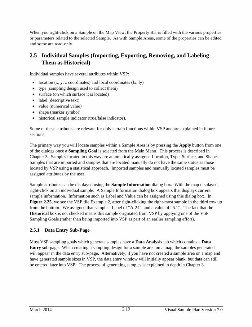
March 2014 Visual Sample Plan Version 7.0 2.19
When you right-click on a Sample on the Map View, the Property Bar is filled with the various properties
or parameters related to the selected Sample. As with Sample Areas, some of the properties can be edited
and some are read-only.
2.5 Individual Samples (Importing, Exporting, Removing, and Labeling
Them as Historical)
Individual samples have several attributes within VSP:
location (x, y, z coordinates) and local coordinates (lx, ly)
type (sampling design used to collect them)
surface (on which surface it is located)
label (descriptive text)
value (numerical value)
shape (marker symbol)
historical sample indicator (true/false indicator).
Some of these attributes are relevant for only certain functions within VSP and are explained in future
sections.
The primary way you will locate samples within a Sample Area is by pressing the Apply button from one
of the dialogs once a Sampling Goal is selected from the Main Menu. This process is described in
Chapter 3. Samples located in this way are automatically assigned Location, Type, Surface, and Shape.
Samples that are imported and samples that are located manually do not have the same status as those
located by VSP using a statistical approach. Imported samples and manually located samples must be
assigned attributes by the user.
Sample attributes can be displayed using the Sample Information dialog box. With the map displayed,
right-click on an individual sample. A Sample Information dialog box appears that displays current
sample information. Information such as Label and Value can be assigned using this dialog box. In
Figure 2.25, we see the VSP file Example 2, after right-clicking the right-most sample in the third row up
from the bottom. We assigned that sample a Label of “A-24”, and a value of “6.1”. The fact that the
Historical box is not checked means this sample originated from VSP by applying one of the VSP
Sampling Goals (rather than being imported into VSP as part of an earlier sampling effort).
2.5.1 Data Entry Sub-Page
Most VSP sampling goals which generate samples have a Data Analysis tab which contains a Data
Entry sub-page. When creating a sampling design for a sample area on a map, the samples generated
will appear in the data entry sub-page. Alternatively, if you have not created a sample area on a map and
have generated sample sizes in VSP, the data entry window will initially appear blank, but data can still
be entered later into VSP. The process of generating samples is explained in depth in Chapter 3.
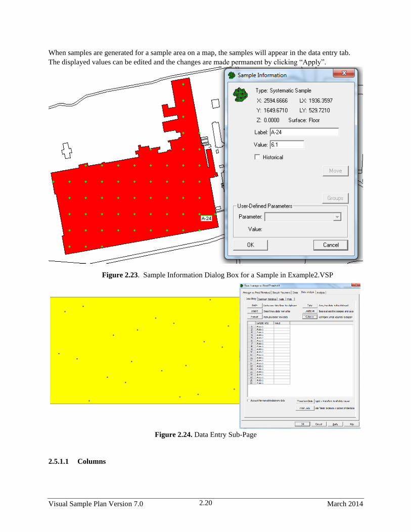
Visual Sample Plan Version 7.0 March 2014 2.20
When samples are generated for a sample area on a map, the samples will appear in the data entry tab.
The displayed values can be edited and the changes are made permanent by clicking “Apply”.
Figure 2.24. Data Entry Sub-Page
2.5.1.1 Columns
Figure 2.23. Sample Information Dialog Box for a Sample in Example2.VSP

March 2014 Visual Sample Plan Version 7.0 2.21
The column configuration may be sparse initially as in
Figure 2.26, but the number of columns displayed can
be expanded by pressing the Columns button to
configure which columns to display. Pressing the
Columns button brings up the Columns Setup window
as shown in Figure 2.27. Columns can be added to the
configuration by selecting the relevant column(s) under
Available Columns and pressing Add. Likewise,
columns can be removed from the configuration by
selecting items under Used Columns and pressing
Remove. Pressing Custom will bring up VSP’s user
defined-parameters dialogue for defining additional
columns. The column definitions are as follows:
Action Limit – The action level or value of concern for an analyte. Usually a value stated in the
sampling goal’s null hypothesis.
Analyte – The name of the chemical or analysis in the sample design and the data analysis. Examples:
Arsenic, Trichloroethylene, etc. When this column is used, each measurement is displayed in a separate
row, and Analyte will refer to what was being measured for that row of data.
Analyte (Name) – Often multiple analytes are displayed in different columns such as in a spreadsheet.
When importing, select “Analyte (<Name of Analyte>)” and you will be prompted to enter the name of
the analyte for each column.
Data Qualifiers – Usually this is a column with information where certain values indicate that values are
non-detects.
Date/Time – The date and time the data was collected.
Location (x,y,z) – The x, y, and z coordinates of the sample.
Location ID – An ID unique to each sample. Using sample IDs is the best way to assure data is imported
into VSP correctly.
Value – the measured value for an analyte.
X coordinate – The coordinate measured along the x axis, or left-to-right direction on a map.
Y coordinate – The coordinate measured along the y axis, or bottom-to-top direction on a map.
Z coordinate – The coordinate measured along the z axis, or height direction.
Possible outlier – This identifies values which stand out from the main group of values – usually
identified by a specific test.
Figure 2.25 Columns Setup

Visual Sample Plan Version 7.0 March 2014 2.22
Predicted – In modules involving trends over time, if a model generated outside of VSP yielded
predicted values, these can be imported into VSP using this column distinction.
Sample area – This identifies the sample area in which a sample is located.
Set - For mean vs. reference designs, this indicates whether the sample belongs to the reference area (R)
or the study unit (S, S1, S2, etc.).
Units -Indicates the measurement units (ug/L, mg/kg, ppm, etc.) associated with the Value.
2.5.1.2 Copy
If the data entry tab is populated with sample information, clicking the Copy button will copy the
displayed columns into a tab delimited format which can be pasted into a spreadsheet or text file. This is
often done after a sampling design is generated to export the sample locations outside of VSP.
2.5.1.3 Delete All
Selecting Delete All and then clicking Apply will remove all of the data from the data entry tab. This is
available for cases where samples collected differ from the VSP sampling design and it is easiest to clear
VSP’s sample information and import the new data. Note that this will also delete sample locations from
the map.
2.5.1.4 Paste
If data outside of VSP is in a tab delimited format (usually the default format in a spreadsheet), it can be
pasted into VSP by selecting and copying the data outside of VSP, then clicking the Paste button in the
data entry tab. The data copied from a spreadsheet (Figure 2.28, left) will be displayed in VSP in the
Add Data window (Figure 2.28, right) where columns and row specifications are made.
Figure 2.26 Spreadsheet Data Pasted Into VSP

March 2014 Visual Sample Plan Version 7.0 2.23
In the Add Data window, if the first
row is a header row, clicking the
“Ignore header row during import”
box at the top of the window will
hide it and ignore it when importing
data. When importing data into
VSP, the column names are initially
labeled “Ignore Column” (in red text
in Figure 2.28, right). Clicking on
these column names brings up a list
of the available column names in
VSP from which to select from as
shown in Figure 2.29. Leaving a
column name as “Ignore Column”
means it will not be imported. When
the desired columns have been
assigned their column names, clicking OK will import the data and display it in the data entry tab.
When sample data contains multiple analytes, and the analytes’ measured values are in separate columns
like in the spreadsheet shown in Figure 2.30, left, the “Data contains multiple analyte entries per row”
option at the top of the Add Data window can be checked to simplify data entry. When this box is
checked, “Analyte (Named)” can be selected for the column name(s) as shown in Figure 2.30, right, and
VSP will prompt the user for the analyte’s name as shown in Figure 2.31. The name can either be typed
or can be selected by clicking the drop down button.
Figure 2.28 Analyte Data in Multiple Columns
Some important distinctions when pasting or importing data into VSP are:
Previously existing samples already in VSP will not be deleted.
Imported samples will be merged with existing samples if their information is the same.
Generally this occurs only if the imported data appends the old data, such as filling in a blank. If
any non-blank fields differ, VSP will treat the new data as a separate sample and will not merge
the two.
Figure 2.27 Column Names to Select From

Visual Sample Plan Version 7.0 March 2014 2.24
2.5.1.5 Import
Clicking Import works much the same way as
using Paste, with the exception being that you
select a file to import rather than pasting the data
in. The file must be a text file in tab delimited
format. After clicking Import, the Import Date
File window will open (Figure 2.32, left) and you
must locate the file, select it, and click Open. The
data will then be displayed in the Add Data
window (Figure 2.32, right), and from there the process is the same as it is when using Paste.
Figure 2.30 Import Data File
2.5.1.6 Manual Data Entry
Clicking the Manual button allows for manual entry of data into VSP. This will bring up an Add data
window which contains the columns currently being displayed in the data entry tab (Figure 2.33, left).
The cells can be populated by clicking on the individual cells. When clicking on a cell, you will be
prompted to either type in the value or select items from a drop down list (Figure 2.33, right).
Figure 2.31 Manual Data Entry
Figure 2.29 Enter Analyte Name

March 2014 Visual Sample Plan Version 7.0 2.25
2.5.1.7 Transform Data
Clicking the Transform Data button allows for the raw values to be transformed by taking either the
natural or base 10 logarithm of the raw value.
2.5.1.8 Filter Data
Clicking the Filter Data button allows for only a subset of the data that meets certain parameters to be
used.
2.5.1.9 Analytes Tab and Multiple Analytes
An adjacent tab to the Data Entry tab is the Analytes tab. This tab displays all of the analytes associated
with the VSP project. Many sampling problems involve only one analyte, but this tab exists for cases
where many variables are being measured, not just one. Analytes can either be entered manually in the
analytes tab, or when importing data, if analytes are read in that aren’t in the analytes tab, these are added
automatically.
2.5.2 Other Ways of Importing Samples
There are two other ways to import sampling locations without using the Data Entry sub-page:
1. Copy them from the Windows Clipboard. Edit the coordinates in a text editor, a word processor, or a
spreadsheet. Each line (or row) represents a different sampling location. The first column is the x
coordinate; the second column is the y coordinate. The third column is the sample Type and is
optional. Valid sample Types are Random, Systematic, Hotspot, Manual, Adaptive-Fill, Unknown,
Transect, Compliance Transect, Meandering Transect, Ranked Set, Cluster, Grid Cell, Perimeter,
Collaborative, Hot Spot Cell, and Increment. The fourth column is the sample label and is optional.
Spaces or tabs should separate columns. (Tabs are preferable.) The coordinates must lie inside a
selected Sample Area.
Example: Type the following coordinates into a text editor such as Notepad:
10 10 Random
50 10 Systematic
10 50 Hotspot
95 60 Manual
99 99 Adaptive-Fill
150 150 Unknown
Now press Ctrl-A to select all the text and Ctrl-C to copy the text to the Windows Clipboard. Run VSP
and load OneAcre.Vsp. Select the Main Menu option View > Coordinates. Paste the coordinates into
VSP using either Ctrl-V or Main Menu option Edit > Paste. View the new sampling locations using the
Main Menu options View > Map or Window > Quad Window. Your map view should now look like
Figure 2.34.

Visual Sample Plan Version 7.0 March 2014 2.26
Figure 2.32. The OneAcre.VSP Project with Sampling Locations Added from Windows Clipboard
You can place the mouse on any sample point and right-click to see the attributes of the sample at that
sample Location. Figure 2.35 shows the Sample Information VSP has for the sample near the arrow.
2. Import sampling locations from a text file. The text file must be formatted as described above.
Choose Main Menu option Map > Sample Points > Import and enter the file name in the dialog
box.
Samples that are imported are assigned Shapes depending on the Type attribute assigned. Sample Type
can be edited by selecting Edit > Samples > Shapes from the Main Menu. A newer, preferred method of
changing the sample shapes is by using the menu Edit > Samples > Symbols. The Dialog box that
appears shows both the shapes assigned to valid Types (use the pull-down menu to select among valid
Types), and gives a picture of the Shape. Figure 2.35 shows that when a sample was collected according
to a Manual design, it will be displayed with a Small Square within a Large X Shape.

March 2014 Visual Sample Plan Version 7.0 2.27
Figure 2.33. Example of Sample Information Box
2.5.3 Historical Samples
Sample locations with the Historical box checked have a unique role in VSP. VSP gives you “credit” for
them in accounting for the total number of new samples needed. This is explained in Section 3.2. The
important point to remember here is that if you import samples, manually add samples, or have a
sampling design previously created within VSP, you can give specific samples a “Historical” status by
placing your mouse over the sample location while in Map View and, in the dialog that comes up,
checking the Historical box. The historical flag can be changed for individual samples from the sample
information dialog box. Edit > Samples > Mark All Historical turns on the historical flag of all samples
in all selected sample areas.
2.5.4 Another Way of Exporting Sampling Locations
Besides using the Copy button in the Data Entry sub-page and pasting into a program outside of VSP,
there is another method of exporting sampling locations. To export sampling locations to a text file (for
example, to use the coordinates in a ground penetrating radar system),
1. Select the Sample Area as described above and develop the sampling design as described in
Section 3.
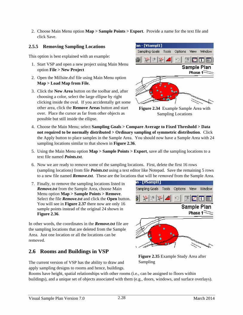
Visual Sample Plan Version 7.0 March 2014 2.28
2. Choose Main Menu option Map > Sample Points > Export. Provide a name for the text file and
click Save.
2.5.5 Removing Sampling Locations
This option is best explained with an example:
1. Start VSP and open a new project using Main Menu
option File > New Project
2. Open the Millsite.dxf file using Main Menu option
Map > Load Map from File.
3. Click the New Area button on the toolbar and, after
choosing a color, select the large ellipse by right
clicking inside the oval. If you accidentally get some
other area, click the Remove Areas button and start
over. Place the cursor as far from other objects as
possible but still inside the ellipse.
4. Choose the Main Menu; select Sampling Goals > Compare Average to Fixed Threshold > Data
not required to be normally distributed > Ordinary sampling of symmetric distribution. Click
the Apply button to place samples in the Sample Area. You should now have a Sample Area with 24
sampling locations similar to that shown in Figure 2.36.
5. Using the Main Menu option Map > Sample Points > Export, save all the sampling locations to a
text file named Points.txt.
6. Now we are ready to remove some of the sampling locations. First, delete the first 16 rows
(sampling locations) from file Points.txt using a text editor like Notepad. Save the remaining 5 rows
to a new file named Remove.txt. These are the locations that will be removed from the Sample Area.
7. Finally, to remove the sampling locations listed in
Remove.txt from the Sample Area, choose Main
Menu option Map > Sample Points > Remove.
Select the file Remove.txt and click the Open button.
You will see in Figure 2.37 there now are only 16
sample points instead of the original 24 shown in
Figure 2.36.
In other words, the coordinates in the Remove.txt file are
the sampling locations that are deleted from the Sample
Area. Just one location or all the locations can be
removed.
2.6 Rooms and Buildings in VSP
The current version of VSP has the ability to draw and
apply sampling designs to rooms and hence, buildings.
Rooms have height, spatial relationships with other rooms (i.e., can be assigned to floors within
buildings), and a unique set of objects associated with them (e.g., doors, windows, and surface overlays).
Figure 2.35 Example Study Area after
Sampling
Figure 2.34 Example Sample Area with
Sampling Locations

March 2014 Visual Sample Plan Version 7.0 2.29
They also have a unique set of parameters that are VSP-assigned (e.g., volume, floors, ceilings, walls) and
user-assigned (e.g., zones, class, HVAC system, release point of threat agent, etc.).
At the most basic level, a Room is just an enclosed Sample Area with height greater than zero. As such,
many of the VSP functions and screens associated with Sample Areas are the same for Rooms. However,
there are also many VSP functions used exclusively for Rooms.
A Building is a collection of rooms. A Building is input into VSP by loading a .dxf map file. To place
multiple floors of buildings in a VSP project: load each floor from a separate .dxf file, giving each file a
different z-offset when loading. Rooms, stairways, and elevators within the building upon which you
wish to place samples need to be defined to VSP by using the Room > Delineate Rooms function.
Alternatively, simply a create sample area that follows the outline of a room or a stairwell on the CAD
drawing (i.e., a floor plan .dxf file) to define room shape and size (see section 2.3.1.1, corner selection
method) and then change the room height to a value greater than 0. See Chapter 6 Room Features in VSP
for more information.
2.6.1 Drawing a Room
Start a new project using Main Menu option File > New Project. Click the Draw Room button on the
Room Toolbar or select Main Menu option Room > Draw. (Use View / Room Toolbar to show the
Room Toolbar.) A tooltip box displays the three ways to draw a room using this tool:
Enter the room dimensions on the keyboard: LxWxH. (e.g., 12x10x8 <enter>)
Enter the corners of the room on the keyboard: X, Y (e.g., 50, 50 <enter> 90,90 <enter>).
Left-click the mouse at the upper-left hand corner of the room, and drag the mouse to the lower-right
hand corner. Left-click the mouse to finish the room. This is similar to drawing a rectangle, except
that VSP automatically sets a wall height of 8 ft. Room height can be changed using Main Menu
item Room > Set Room Height or by clicking on the Set Height button on the drawing toolbar.
With the room displayed, right-click anywhere within the room. The Sample Area Information dialog
box appears (Figure 2.38).
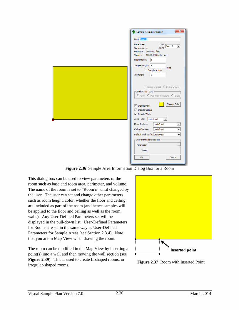
Visual Sample Plan Version 7.0 March 2014 2.30
Figure 2.36 Sample Area Information Dialog Box for a Room
This dialog box can be used to view parameters of the
room such as base and room area, perimeter, and volume.
The name of the room is set to “Room n” until changed by
the user. The user can set and change other parameters
such as room height, color, whether the floor and ceiling
are included as part of the room (and hence samples will
be applied to the floor and ceiling as well as the room
walls). Any User-Defined Parameters set will be
displayed in the pull-down list. User-Defined Parameters
for Rooms are set in the same way as User-Defined
Parameters for Sample Areas (see Section 2.3.4). Note
that you are in Map View when drawing the room.
The room can be modified in the Map View by inserting a
point(s) into a wall and then moving the wall section (see
Figure 2.39). This is used to create L-shaped rooms, or
irregular-shaped rooms. Figure 2.37 Room with Inserted Point
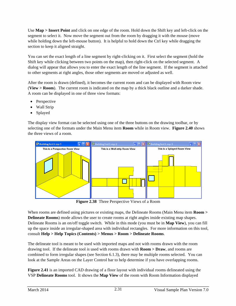
March 2014 Visual Sample Plan Version 7.0 2.31
Use Map > Insert Point and click on one edge of the room. Hold down the Shift key and left-click on the
segment to select it. Now move the segment out from the room by dragging it with the mouse (move
while holding down the left-mouse button). It is helpful to hold down the Ctrl key while dragging the
section to keep it aligned straight.
You can set the exact length of a line segment by right-clicking on it. First select the segment (hold the
Shift key while clicking between two points on the map), then right-click on the selected segment. A
dialog will appear that allows you to enter the exact length of the line segment. If the segment is attached
to other segments at right angles, those other segments are moved or adjusted as well.
After the room is drawn (defined), it becomes the current room and can be displayed with Room view
(View > Room). The current room is indicated on the map by a thick black outline and a darker shade.
A room can be displayed in one of three view formats:
Perspective
Wall Strip
Splayed
The display view format can be selected using one of the three buttons on the drawing toolbar, or by
selecting one of the formats under the Main Menu item Room while in Room view. Figure 2.40 shows
the three views of a room.
Figure 2.38 Three Perspective Views of a Room
When rooms are defined using pictures or existing maps, the Delineate Rooms (Main Menu item Room >
Delineate Rooms) mode allows the user to create rooms at right angles inside existing map shapes.
Delineate Rooms is an on/off toggle switch. While in this mode (you must be in Map View), you can fill
up the space inside an irregular-shaped area with individual rectangles. For more information on this tool,
consult Help > Help Topics (Contents) > Menus > Room > Delineate Rooms.
The delineate tool is meant to be used with imported maps and not with rooms drawn with the room
drawing tool. If the delineate tool is used with rooms drawn with Room > Draw, and rooms are
combined to form irregular shapes (see Section 6.1.3), there may be multiple rooms selected. You can
look at the Sample Areas on the Layer Control bar to help determine if you have overlapping rooms.
Figure 2.41 is an imported CAD drawing of a floor layout with individual rooms delineated using the
VSP Delineate Rooms tool. It shows the Map View of the room with Room Information displayed
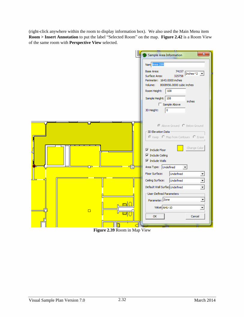
Visual Sample Plan Version 7.0 March 2014 2.32
(right-click anywhere within the room to display information box). We also used the Main Menu item
Room > Insert Annotation to put the label “Selected Room” on the map. Figure 2.42 is a Room View
of the same room with Perspective View selected.
Figure 2.39 Room in Map View
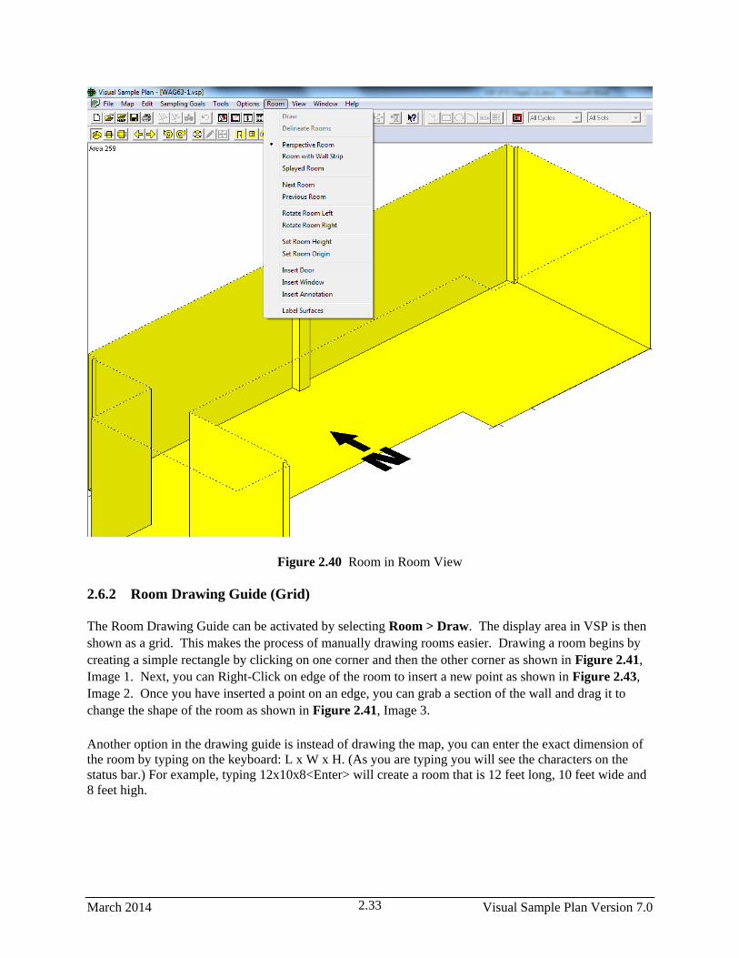
March 2014 Visual Sample Plan Version 7.0 2.33
Figure 2.40 Room in Room View
2.6.2 Room Drawing Guide (Grid)
The Room Drawing Guide can be activated by selecting Room > Draw. The display area in VSP is then
shown as a grid. This makes the process of manually drawing rooms easier. Drawing a room begins by
creating a simple rectangle by clicking on one corner and then the other corner as shown in Figure 2.41,
Image 1. Next, you can Right-Click on edge of the room to insert a new point as shown in Figure 2.43,
Image 2. Once you have inserted a point on an edge, you can grab a section of the wall and drag it to
change the shape of the room as shown in Figure 2.41, Image 3.
Another option in the drawing guide is instead of drawing the map, you can enter the exact dimension of
the room by typing on the keyboard: L x W x H. (As you are typing you will see the characters on the
status bar.) For example, typing 12x10x8<Enter> will create a room that is 12 feet long, 10 feet wide and
8 feet high.

Visual Sample Plan Version 7.0 March 2014 2.34
Figure 2.41. Room Drawing Guide
2.6.3 Extended Room Features
2.6.3.1 Room Objects
VSP has two objects associated with rooms: doors and windows. There are two ways to view these
objects: in Map View (see Figure 2.44) and in Room View (see Figure 2.45). Figure 2.45 is another
section of the CAD drawing shown in Figure 2.42. A door in the CAD drawing was defined for VSP.
Right-clicking on the Map where the arrow is pointing brings up the Object Information dialog box for
the Door Object at that location.

March 2014 Visual Sample Plan Version 7.0 2.35
Figure 2.42 Door Object Displayed Using Map View
Doors and windows can be added in Room View using Main Menu item Room > Insert Door/Window
or by clicking on the door or window button on the Room Toolbar. Once added, the properties of the
room objects can be viewed by right-clicking on the object, which brings up the Object Information
dialog box. This is shown for a door in Figure 2.45 and for a window in Figure 2.46.
Note that VSP also has the capability to place a polygon on top of a surface with a different surface type.
The polygons are called “Surface Overlays”. Surface overlays can be elevated above the floor to
represent the top of furniture, such as a table top. Surface overlays are covered in section 6.3.4.
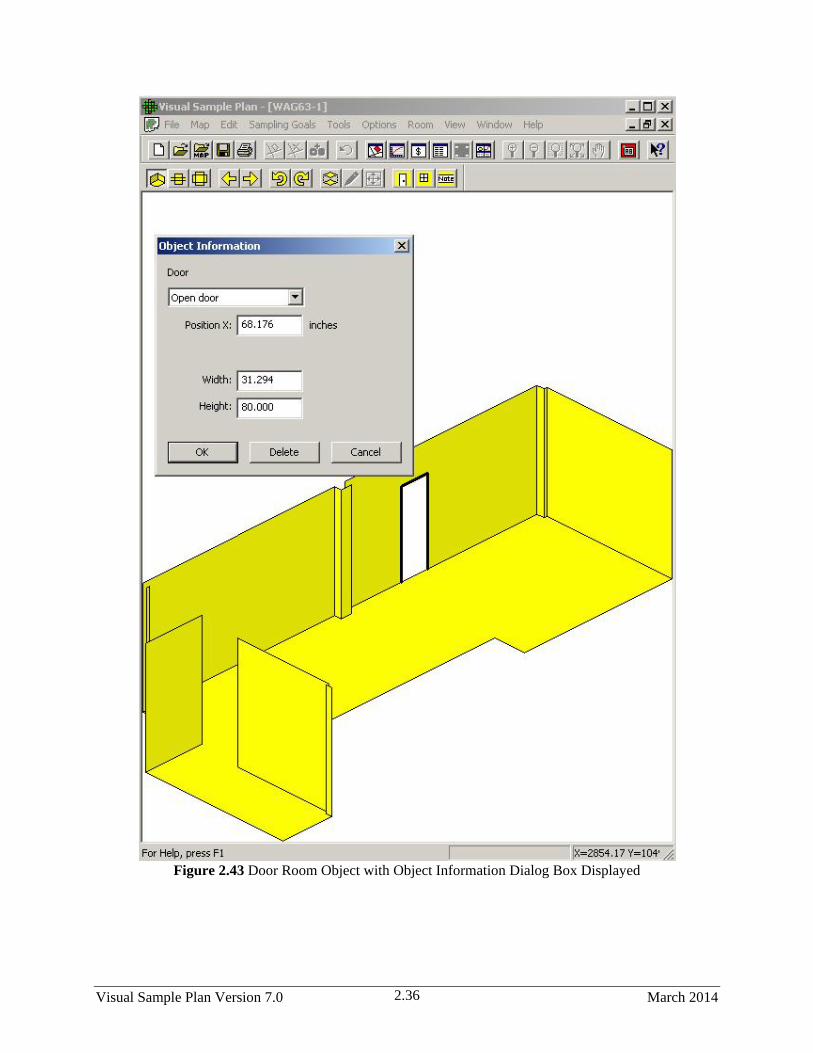
Visual Sample Plan Version 7.0 March 2014 2.36
Figure 2.43 Door Room Object with Object Information Dialog Box Displayed

March 2014 Visual Sample Plan Version 7.0 2.37
Figure 2.44 Window Room Object with Object Information Dialog Box Displayed

Visual Sample Plan Version 7.0 March 2014 2.38
2.6.3.2 Room Parameters
Rooms can have VSP-defined parameters (e.g., Area, Perimeter, Volume, Name) and User-Defined
Parameters (e.g., Zone, Class). The User-Defined Parameters are set in the Sample Area Information
dialog box or with the Main Menu item Edit > Sample Areas > Set Parameter Values. This second
option is a very powerful tool. Figure 2.41 shows that the room named “Area 259” is in Zone “AHU-10”
(i.e., Air Handling Unit 10). All the rooms on AHU 10 are assigned to the same Zone so they are easily
identifiable. In another example, rooms that exceed a release criteria could have a logical (yes/no)
parameter assigned called “Contaminated”, and coded red/green. Note that once a room parameter is set
up using Main Menu item Edit > Sample Areas > User-defined Parameters, all rooms are given a
default value for that parameter. Section 2.3.4 discusses Sample Area Parameters, which also applies to
Rooms.
2.6.3.3 Room Color by Parameter
Rooms can be colored automatically based on the value of one of the built-in or user-defined parameters.
Once rooms have been defined to VSP, choosing the menu item Edit > Sample Areas > Color by Value
displays the dialog shown in Figure 2.47. This dialog allows you to choose one of the predefined
gradient or discrete color sets and one of the sample area parameters. Certain parameters can also be
colored by the logarithm of the value. This dialog also allows the Color by Value function to be turned
off or on. Use the Help button on the toolbar to find out more information on this tool.
Figure 2.45 Dialog Box for Color Sample Areas by Value

March 2014 Visual Sample Plan Version 7.0 2.39
2.6.3.4 Room Order
Clicking the button for Next Room from the Room Toolbar, or selecting Room > Next Room from the
Main Menu changes the current room to the next selected room on the map. The current room is
indicated by a thick black border and is a slightly darker hue in color-coded rooms. Previous Room
changes the current room to the previously selected room on the map. The order of room selection is the
order of creation. Note that the order for room and sample areas can be changed by the menu command
Edit / Sample Areas / Bring to Front.
2.6.3.5 Room Rotation
Clicking the button for Rotate Room Right from the Room Toolbar, or selecting Room > Rotate Room
Right from the Main Menu rotates the Perspective or Wall-Strip Room View clockwise 90 degrees.
Rotate Room Left rotates the Perspective or Wall-Strip Room View counter-clockwise 90 degrees.
2.6.4 Furniture and Stairs
The Furniture / Stairs Menu is accessed by selecting Edit > Furniture / Stairs. The Furniture / Stairs
menu offers the following commands:
Edit Library Furniture / Stairs Object
Edit an existing Furniture or Stairs object file.
New Library Furniture Object
Create a new Furniture object and save it to a file.
New Stairs Object
Create a new Stairs object and save it to a file.
Insert Furniture / Stairs Object into Room
Select a Furniture or Stairs object from a file and insert it into a room.
Furniture Editor
2.6.4.1 Edit LibraryFurniture / Stairs Object
Selecting Edit > Furniture / Stairs > Edit Library Furniture / Stairs Object is used to select an
existing Furniture or Stairs object from an XML file and edit it in the Furniture Editor or Stairs Editor,
respectively. When you close the Furniture or Stairs Editor, you can save the object into a new or
existing XML file. The default location of these object XML files is in the Program Files / Visual Sample
Plan / Furniture folder. These object XML files can be freely exchanged with other VSP users. After the
file is saved, you can use the Insert Furniture / Stairs Object into Room command to select the XML file
(or any other Furniture or Stairs object that has been saved to an XML file) into the Room View.
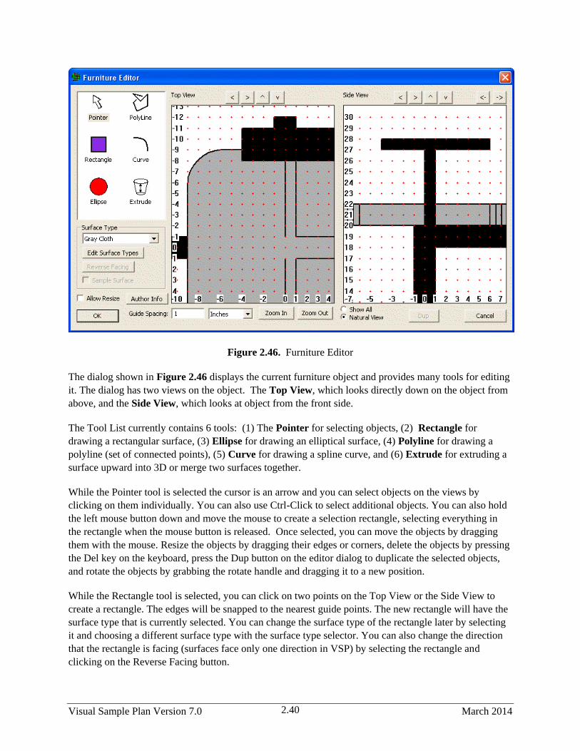
Visual Sample Plan Version 7.0 March 2014 2.40
Figure 2.46. Furniture Editor
The dialog shown in Figure 2.46 displays the current furniture object and provides many tools for editing
it. The dialog has two views on the object. The Top View, which looks directly down on the object from
above, and the Side View, which looks at object from the front side.
The Tool List currently contains 6 tools: (1) The Pointer for selecting objects, (2) Rectangle for
drawing a rectangular surface, (3) Ellipse for drawing an elliptical surface, (4) Polyline for drawing a
polyline (set of connected points), (5) Curve for drawing a spline curve, and (6) Extrude for extruding a
surface upward into 3D or merge two surfaces together.
While the Pointer tool is selected the cursor is an arrow and you can select objects on the views by
clicking on them individually. You can also use Ctrl-Click to select additional objects. You can also hold
the left mouse button down and move the mouse to create a selection rectangle, selecting everything in
the rectangle when the mouse button is released. Once selected, you can move the objects by dragging
them with the mouse. Resize the objects by dragging their edges or corners, delete the objects by pressing
the Del key on the keyboard, press the Dup button on the editor dialog to duplicate the selected objects,
and rotate the objects by grabbing the rotate handle and dragging it to a new position.
While the Rectangle tool is selected, you can click on two points on the Top View or the Side View to
create a rectangle. The edges will be snapped to the nearest guide points. The new rectangle will have the
surface type that is currently selected. You can change the surface type of the rectangle later by selecting
it and choosing a different surface type with the surface type selector. You can also change the direction
that the rectangle is facing (surfaces face only one direction in VSP) by selecting the rectangle and
clicking on the Reverse Facing button.
March 2014 Visual Sample Plan Version 7.0 2.41
While the Ellipse tool is selected, you can click on two points on the Top View or the Side View to create
an ellipse. The edges will be snapped to the nearest guide points. The new ellipse will have the surface
type that is currently selected. You can change the surface type of the ellipse later by selecting it and
choosing a different surface type with the surface type selector. You can also change the direction that the
ellipse is facing (surfaces face only one direction in VSP) by selecting the ellipse and clicking on the
Reverse Facing button.
While the PolyLine tool is selected, you can click on successive points in either View to build up a
polyline. To finish drawing the polyline, Right-Click with the mouse or move the mouse out of the View
box. Each point is snapped to the nearest guide point on the view. If the last point is joined back to the
first point, it becomes an enclosed polygon (also known as a surface). The new polyline will have the
surface type that is currently selected. You can change the surface type of the polyline later by selecting it
and choosing a different surface type with the surface type selector. If the polyline is an enclosed polygon
(surface), you can also change the direction that the surface is facing (surfaces face only one direction in
VSP) by selecting the surface and clicking on the Reverse Facing button.
While the Curve tool is selected, you can click on two end points in either View then click on a third point
to control the amount of curve. The points are snapped to the nearest guide point on the view. If the end
point of the curve is joined to the end of another curve or polyline it becomes part of the polyline. If the
polyline joins its beginning and end points, it becomes an enclosed polygon (also known as a surface).
The new curve will have the surface type that is currently selected. You can change the surface type of the
curve later by selecting it and choosing a different surface type with the surface type selector.
The function of the Extrude tool depends on how many objects are selected before the Extrude tool is
selected. If you first select two objects then select the Extrude tool, when you click the extrude tool it will
create vertical surfaces to join the two objects together. Note that the extrusion is a vertical operation, so
the two selected objects must be separated horizontally. InFigure 2.49, there are two circles selected. The
first circle has a 6 inch radius and is located at Z=0. The second circle has an 8 inch radius and is located
at Z=16.

Visual Sample Plan Version 7.0 March 2014 2.42
Figure 2.47. Example of Two Objects in Extrude Tool
Clicking the Extrude tool creates all the vertical surfaces to join them together. (Click the Natural View
option to see all the surfaces pointing out as shown in Figure 2.48).
Figure 2.48. Natural View
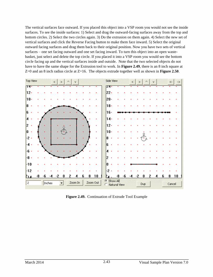
March 2014 Visual Sample Plan Version 7.0 2.43
The vertical surfaces face outward. If you placed this object into a VSP room you would not see the inside
surfaces. To see the inside surfaces: 1) Select and drag the outward-facing surfaces away from the top and
bottom circles. 2) Select the two circles again. 3) Do the extrusion on them again. 4) Select the new set of
vertical surfaces and click the Reverse Facing button to make them face inward. 5) Select the original
outward facing surfaces and drag them back to their original position. Now you have two sets of vertical
surfaces – one set facing outward and one set facing inward. To turn this object into an open waste-
basket, just select and delete the top circle. If you placed it into a VSP room you would see the bottom
circle facing up and the vertical surfaces inside and outside. Note that the two selected objects do not
have to have the same shape for the Extrusion tool to work. In Figure 2.49, there is an 8 inch square at
Z=0 and an 8 inch radius circle at Z=16. The objects extrude together well as shown in Figure 2.50.
Figure 2.49. Continuation of Extrude Tool Example

Visual Sample Plan Version 7.0 March 2014 2.44
Figure 2.50. Natural View of Two Objects Extruded Together
If only one object is selected before selecting the Extrude tool (Figure 2.51, Figure 2.52), the extrusion
works differently. Press down the mouse button in the Side view and drag the points up and down. When
you release the mouse button, the vertical faces will be created. If you hold the Shift key down during
this operation, the vertical faces will be extruded to a single point, creating a cone of sorts.

March 2014 Visual Sample Plan Version 7.0 2.45
Figure 2.51. One object selected in Extrude Tool
Figure 2.52. Natural View of One Object in Extrude Tool

Visual Sample Plan Version 7.0 March 2014 2.46
2.6.4.2 New Library Furniture Object
Selecting Edit > Furniture / Stairs > New Library Furniture Object is used to create a blank Furniture
object and begin editing it in the Furniture Editor. When you close the Furniture Editor, you can save the
new Furniture object into an XML file. The default location of these Furniture XML files is in the
Program Files / Visual Sample Plan / Furniture folder. These Furniture XML files can be freely
exchanged with other VSP users. After the file is saved, you can use the Insert Furniture Object into
Room command to select the XML file (or any other Furniture or Stairs object that has been saved to an
XML file) into the Room View.
2.6.4.3 New Stairs Object
There are no existing stair objects installed with VSP, so they have to be created by the user. Selecting
Edit > Furniture / Stairs > New Stairs Object is used to create a blank Stairs object and begin editing it
in the Stairs Editor. When you close the Stairs Editor, you can save the new Stairs object into an XML
file. The default location of these Stairs XML files is in the Program Files / Visual Sample Plan /
Furniture folder. These Stairs XML files can be freely exchanged with other VSP users. After the file is
saved, you can use the Insert Furniture / Stairs Object into Room command to select the XML file (or any
other Furniture or Stairs object that has been saved to an XML file) into the Room View.
2.6.4.4 Insert Furniture / Stairs Object into Room
Selecting Edit > Furniture / Stairs > Insert Furniture / Stairs Object into Room is used to select a
Furniture object or Stairs object from an XML file and place it in the room. By default, the Furniture /
Stairs object XML files are located in the Program Files / Visual Sample Plan / Furniture folder. Furniture
/ Stairs object XML files can be freely exchanged with other VSP users.
After selecting the XML file, a wire-frame representation appears in the Room View allowing you to
position the object where you want it. When it is properly positioned, click the Mouse Button to place the
object in the room. If the Drawing Guide (Snap-to grid) is turned on, the placement will be aligned to the
grid.
After the Furniture / Stairs object is placed in the room, you can click on the object to highlight it. Once
highlighted, you can drag it to a new position, rotate it to a different orientation or completely delete it
(remove it from the room).
You can also right-click on a Furniture / Stairs object to change some of its location and sampling
attributes or delete it.

March 2014 Visual Sample Plan Version 7.0 2.47
2.7 Surface Overlays
One or more surface overlays can be
inserted in a room to represent a portion of
a surface that needs to be distinguished
from the overall surface. For example, a
portion of the floor in a room may be
covered with tile while most of the floor is
covered with carpet, requiring a different
sampling technique. A surface overlay can
be elevated from the floor to represent the
top horizontal surface of a desk, chair,
cabinet, or shelf. Surface overlays can be
placed on any surface in the room. Only
floor overlays can be elevated.
When starting a VSP project, the only
surface type available is the default
“undefined” surface type. To define
additional surface types, select Edit >
Surfaces > Surface Type to bring up the
Edit Surface Types dialog (Figure 2.55).
This dialog is used to define different
surface types that can be assigned to the
surfaces (floor, ceiling, walls, etc.) inside a
room or to surface overlays. Click on an
existing surface type to change the name or
select different User-Defined Parameters,
or to add a new surface type, click Insert New.
To create a surface overlay, select Edit > Surfaces > Create Surface Overlays. This allows you to
create a small patch on an existing surface (floor, wall, etc.) that can be distinguished from the room
surface on which it is located. See Section 6.3.4 for more information on surface overlays.
2.8 Saving a VSP File
No matter how you imported or created a site map or Sample Area for VSP, you can always save the
information in VSP’s own file format. From the Main Menu, select File > Save Project As and provide a
name for the project. VSP will add the VSP file extension automatically. Alternatively, you can use the
Save button with the disk icon on the VSP toolbar. After you have created a sampling design as
discussed later in this guide, saving your project as a VSP file also will save the input data, cost data, and
recommended sample sizes.
2.9 Help
There are several ways to get Help in VSP:
Figure 2.53. Edit Surface Types Dialog in VSP

Visual Sample Plan Version 7.0 March 2014 2.48
Select Help from the top bar of Menu items for help on the Expert Mentor (section 2.9.1) or to view
Help Topics by Contents, Index, and Search.
Select the Help button on the main toolbar (button to the far right labeled “?”) and click on any pull-
down menu item or other feature on the VSP screen. The Help Topic for that menu selection will be
displayed.
Help button at the bottom of some Dialog Boxes and Input and Output Screens. The Help brings up
a new screen that contains a technical discussion of the tests, algorithms, and calculations used by
VSP to perform the functions referred to on the Input and Output Screens.
VSP is user-friendly and most users find they can run VSP from the guidance and information presented
in the various Help functions in VSP.
2.9.1 Expert Mentor
The Expert Mentor dialog provides guidance, recommendations, and warnings to the VSP user to:
Help prevent inadvertent misuse of VSP
Help the user understand how VSP works
Help ensure the number and location of samples obtained using VSP are appropriate
To activate the Expert Mentor, select Help > Expert Mentor. Figure 2.56 shows the Expert Mentor
dialog.
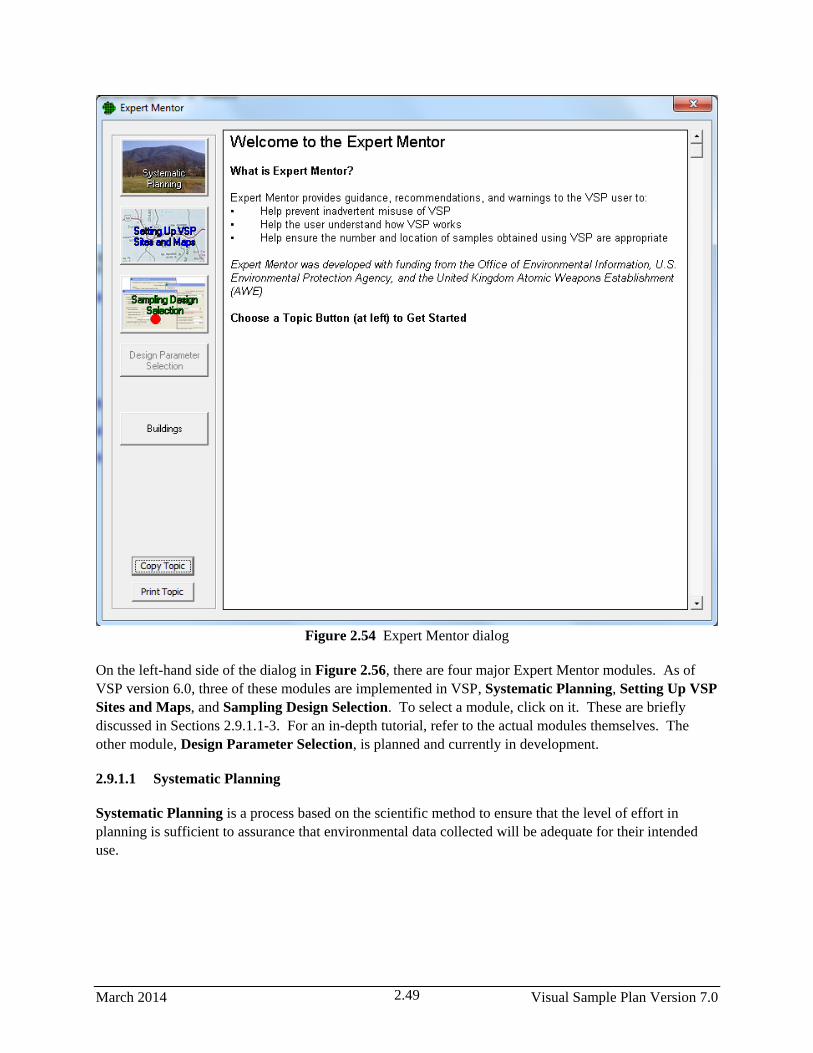
March 2014 Visual Sample Plan Version 7.0 2.49
Figure 2.54 Expert Mentor dialog
On the left-hand side of the dialog in Figure 2.56, there are four major Expert Mentor modules. As of
VSP version 6.0, three of these modules are implemented in VSP, Systematic Planning, Setting Up VSP
Sites and Maps, and Sampling Design Selection. To select a module, click on it. These are briefly
discussed in Sections 2.9.1.1-3. For an in-depth tutorial, refer to the actual modules themselves. The
other module, Design Parameter Selection, is planned and currently in development.
2.9.1.1 Systematic Planning
Systematic Planning is a process based on the scientific method to ensure that the level of effort in
planning is sufficient to assurance that environmental data collected will be adequate for their intended
use.

Visual Sample Plan Version 7.0 March 2014 2.50
Figure 2.55 Systematic Planning dialog
The dialog for Systematic Planning is shown in Figure 2.57. A number of tutorials can be accessed by
clicking on them. These are briefly described below. Note that within each of these topics there are also
one too many subtopics which provide additional information and tutorials. To access these subtopics,
use the Systematic Planning module in the Expert Mentor.
What is it? This explains what systematic planning is.
Why do it? This provides guidance on avoiding bad data, balancing resources and decision uncertainty,
avoiding waste by thinking through why, what, how, and when, assuring VSP is not misused, avoiding
bad or inappropriate data, getting the right amount of representative data, and using the right statistic.
How to do it? This describes the DQO (Data Quality Objectives) process and the Triad Approach for
modernizing and streamlining sampling, analysis, and data management.
Conceptual Site Model (CSM) Development. Explains how to use a Conceptual Site Model that
describes what is known about the site.

March 2014 Visual Sample Plan Version 7.0 2.51
Representative Samples and Measurements. Explains what Representative Samples and
Measurements are, why they are important, and how to achieve them.
Check List of Questions to Ponder During Systematic Planning. Provides a list of questions to go
through to assist in the planning process.
2.9.1.2 Setting Up VSP Sites and Maps
This module explains the process of loading, drawing, and setting up Maps in VSP. The Setting Up VSP
Sites and Maps dialog is shown in Figure 2.58. The sections shown in Figure 2.58 are explained
below.
Figure 2.56 Setting up VSP Sites and Maps dialog
Help on Working with Maps. This section explains a number of topics on how to work with maps.
Topics include an overview, objects in VSP maps, loading maps from a file, creating a map by drawing,
creating a map from coordinates, editing a map, editing a sample area, navigating the map, working with
background pictures, and topics on miscellaneous tools, tips, tricks, and traps.
Step Through the Process. This section allows you to step through the process of setting up a site in
VSP in a systematic fashion. Clicking on the links actually performs or initiates the actions within VSP.

Visual Sample Plan Version 7.0 March 2014 2.52
Topics include starting with a blank project, loading and drawing maps, setting map units, creating a
sample area, and loading a background picture.
2.9.1.3 Sampling Design Selection
The Sampling Design Selection dialog asks the user a series of questions in order to point them to the
relevant module(s) to use based on their answers. The first screen (Figure 2.59) is a list of “needs” where
you check all that apply. The subsequent screens ask you about the assumptions you are making about
the data to be collected. When the needs and assumptions have been defined, Expert Mentor lists the VSP
modules which are relevant given those needs and assumptions.
Figure 2.57 Systematic Planning First Screen
2.9.1.4 Buildings
The Buildings dialog asks the user points the user to a number of options for working with buildings. The
first screen (Figure 2.60) shows several options for working on setting up a building in VSP. The
subsequent screens point to more specific actions.

March 2014 Visual Sample Plan Version 7.0 2.53
Figure 2.58. Buildings First Screen

March 2014 Visual Sample Plan Version 7.0 3.1
3.0 Sampling Plan Development Within VSP
3.1 Sampling Plan Type Selection
Sampling plan components consist of where to take samples, how many samples to take, what kind of
samples (e.g., surface soil, air), and how to take samples and analyze them. We identified the general
areas of where to take samples in Section 2.3, Sample Areas in VSP. In this section, we discuss where
within the Sampling Area to locate the samples. We also discuss how many samples to take. The kind
of samples to take—i.e., soil vs. groundwater, wet vs. dry, surface vs. core,—is determined during Step 3 of
the DQO process (Define Inputs) and is not addressed directly in VSP. The Measurement Quality Objectives
module in VSP (Section 5.4) deals with how the method selected for analytically measuring the sample relates to
other components of the sampling plan.
3.1.1 Defining the Purpose/Goal of Sampling
VSP follows the DQO planning process in directing users in the selection of the components of the sampling
plan. The first thing you must do is to select the type of problem for which the current data collection
effort will be used to resolve. In VSP, we call this the Sampling Goal. The following types of problems
are addressed currently in VSP. Future versions will expand on this list:
Sampling Goal Description
Compare Average to Fixed Threshold Calculate number of samples needed to compare a sample mean or
median against a predetermined threshold and places them on the
map. This is called a one-sample problem.
Compare Average to Reference Average Calculate number of samples needed to compare a sample mean or
median against a reference mean or median and places them on the
map. This is typically used when a reference area has been selected
(i.e., a background area) and the problem is to see if the study area is
equal to, or greater than, the reference area. This is called a two-sample
problem because the data from two sites are compared to each other.
Estimate the Mean Calculate number of samples needed to estimate the population mean
and places them on the map.
Construct Confidence Interval on Mean Calculate number of samples needed to find a confidence interval on a
mean and places them on the map.
Locate Hot Spots Use systematic or approximate grid sampling or multiple increment
sampling to locate a Hot Spot (i.e., small pockets of contamination).
Show that at least some high % of the sampling
area is acceptable
Calculate number of samples needed to confidently show that little if
any contamination is present or exceeds a specified threshold.
Discover Unacceptable Areas with High
Confidence
Develop sampling designs to discover, with high probability,
contaminated areas (unacceptable grid cells) if they exist
Combined Average and Individual Measurement
Criteria
Compares the results of two designs, to see which one requires the
most samples to meet its sampling goals.
Detect a Trend Determine sampling frequency required to detect linear or exponential
trends and tests whether a trend exists for a measurement of interest.
Identify Sampling Redundancy Analyze data to determine whether sampling can be performed less
frequently or in fewer locations without losing important trend or
spatial information.
Add Sampling Locations to Reduce Spatial
Uncertainty
Place additional samples to improve estimates based on a geostatistical
analysis of existing data
Compare Proportion to Fixed Threshold Calculate number of samples needed to compare a proportion to a
given proportion and places them on the map
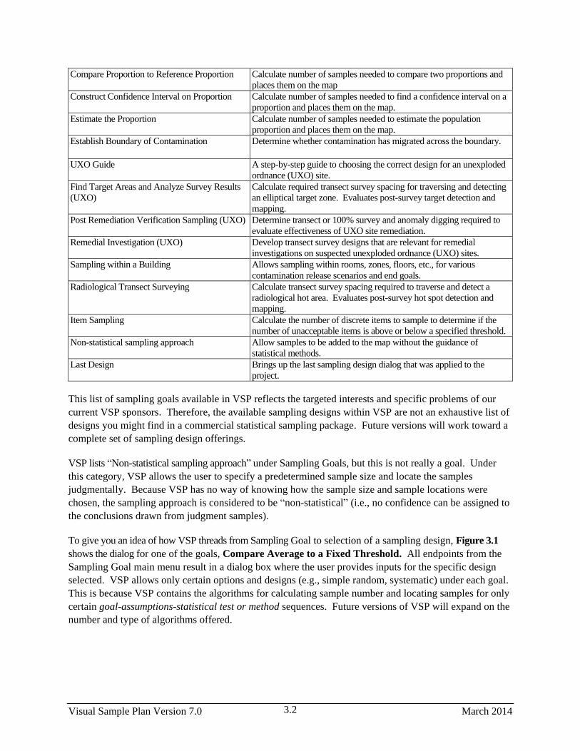
Visual Sample Plan Version 7.0 March 2014 3.2
Compare Proportion to Reference Proportion Calculate number of samples needed to compare two proportions and
places them on the map
Construct Confidence Interval on Proportion Calculate number of samples needed to find a confidence interval on a
proportion and places them on the map.
Estimate the Proportion Calculate number of samples needed to estimate the population
proportion and places them on the map.
Establish Boundary of Contamination Determine whether contamination has migrated across the boundary.
UXO Guide A step-by-step guide to choosing the correct design for an unexploded
ordnance (UXO) site.
Find Target Areas and Analyze Survey Results
(UXO)
Calculate required transect survey spacing for traversing and detecting
an elliptical target zone. Evaluates post-survey target detection and
mapping.
Post Remediation Verification Sampling (UXO) Determine transect or 100% survey and anomaly digging required to
evaluate effectiveness of UXO site remediation.
Remedial Investigation (UXO) Develop transect survey designs that are relevant for remedial
investigations on suspected unexploded ordnance (UXO) sites.
Sampling within a Building Allows sampling within rooms, zones, floors, etc., for various
contamination release scenarios and end goals.
Radiological Transect Surveying Calculate transect survey spacing required to traverse and detect a
radiological hot area. Evaluates post-survey hot spot detection and
mapping.
Item Sampling Calculate the number of discrete items to sample to determine if the
number of unacceptable items is above or below a specified threshold.
Non-statistical sampling approach Allow samples to be added to the map without the guidance of
statistical methods.
Last Design Brings up the last sampling design dialog that was applied to the
project.
This list of sampling goals available in VSP reflects the targeted interests and specific problems of our
current VSP sponsors. Therefore, the available sampling designs within VSP are not an exhaustive list of
designs you might find in a commercial statistical sampling package. Future versions will work toward a
complete set of sampling design offerings.
VSP lists “Non-statistical sampling approach” under Sampling Goals, but this is not really a goal. Under
this category, VSP allows the user to specify a predetermined sample size and locate the samples
judgmentally. Because VSP has no way of knowing how the sample size and sample locations were
chosen, the sampling approach is considered to be “non-statistical” (i.e., no confidence can be assigned to
the conclusions drawn from judgment samples).
To give you an idea of how VSP threads from Sampling Goal to selection of a sampling design, Figure 3.1
shows the dialog for one of the goals, Compare Average to a Fixed Threshold. All endpoints from the
Sampling Goal main menu result in a dialog box where the user provides inputs for the specific design
selected. VSP allows only certain options and designs (e.g., simple random, systematic) under each goal.
This is because VSP contains the algorithms for calculating sample number and locating samples for only
certain goal-assumptions-statistical test or method sequences. Future versions of VSP will expand on the
number and type of algorithms offered.
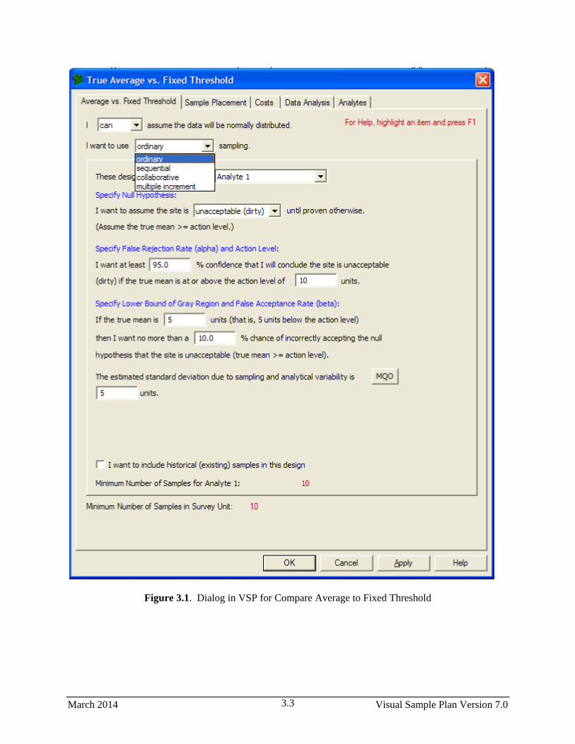
March 2014 Visual Sample Plan Version 7.0 3.3
Figure 3.1. Dialog in VSP for Compare Average to Fixed Threshold

Visual Sample Plan Version 7.0 March 2014 3.4
3.1.2 Selecting a Sampling Design
The current release of VSP offers several versions of the software (see Figure 2.1). Each version has a
unique set of sampling designs available to the user – except General (all inclusive) VSP which contains
all of the designs. Some of the designs available under each of the Sampling Goal menu items are unique
to that goal, while other designs are available under multiple goals. Thus, the Sampling Goal you select
determines which sampling design(s) will be available to you.
If a user is new to VSP, and is not looking for a specific sample design but rather has a general definition
of the problem to be resolved with sample data, a good discussion of how to select a sampling design is in
EPA’s Guide for Choosing a Sampling Design for Environmental Data Collection (EPA 2002)
http://www.epa.gov/quality/qa_docs.html. See Table 3-1 on pages 24-25 in that source for examples of
problem types that one may encounter and suggestions for sampling designs that are relevant for these problem
types in particular situations. Another guidance document, Multi-Agency Radiation Survey and Site
Investigation Manual (MARSSIM) (EPA 1997) http://www.epa.gov/radiation/marssim/, also provides
insight into how to select a sample design. The Expert Mentor in VSP may also be used to assist in
selecting a sampling design by selecting Help > Expert Mentor and then clicking the Sampling Design
Selection button.
One of the valuable ways to use VSP is to run through the various Goals and see what changes from one
Goal to another, what sampling designs are available for each Goal, how designs perform, and what
assumptions are required for each design. This trial and error approach is probably the best way to select a
design that best fits your regulatory environment, unique site conditions, and goals.
An important point to keep in mind is the linkage between 1) the minimum number of samples that must be
collected and where they are located, and 2) how you will analyze the sampling results to calculate
summary values (on which you will base your decisions). The user must understand this linkage in order to
select the appropriate design. Once the samples are collected and analyzed, the statistical tests and
methods assumed in the sample size formulas and design may be used in the analysis phase, Data Quality
Assessment (DQA).
Many of the designs in VSP contain a Data Analysis tab and allow sample results to be input into VSP so
tests can be executed and conclusions drawn based on the results. See Section 5.6 for a discussion of
Data Analysis within VSP.
We cannot discuss all the technical background behind the designs here, but the technical documentation
for VSP gives sample size formulas used in VSP and provides references. The online help in VSP provides
technical help and references. The reports that are available within VSP are a good source for definitions,
assumptions, sample size formulas, and technical justification for the design selected. Finally, the VSP
web site, http://vsp.pnl.gov/, has some technical documentation available, and allows download of the
documents.
VSP allows both probability-based designs and judgmental sampling:
Probability-based sampling designs apply sampling theory and involve random selection. An
essential feature of a probability-based sample is that each member of the population from which
the sample was selected has a known probability of selection. When a probability based design is

March 2014 Visual Sample Plan Version 7.0 3.5
used, statistical inferences may be made about the sampled population from the data obtained
from the sampled units. Judgmental designs involve the selection of sampling units on the basis
of expert knowledge or professional judgment (EPA 2002, pp. 9-10).
The design recommended by VSP depends on the sampling goal selected, assumptions made, and in the
case of Ordinary Sampling, user input provided under the Sample Placement tab. VSP contains the
following two- and three-dimensional designs. With exception to judgment sampling, these are
probability-based designs.
Figure 3.2 Sample Placement for Ordinary Sampling for Selecting Sample Placement Method and Type
Ordinary sampling – two Sample Placement options are available:
1. simple random sampling where sampling locations are selected based on random numbers,
which are then mapped to the spatial locations, and
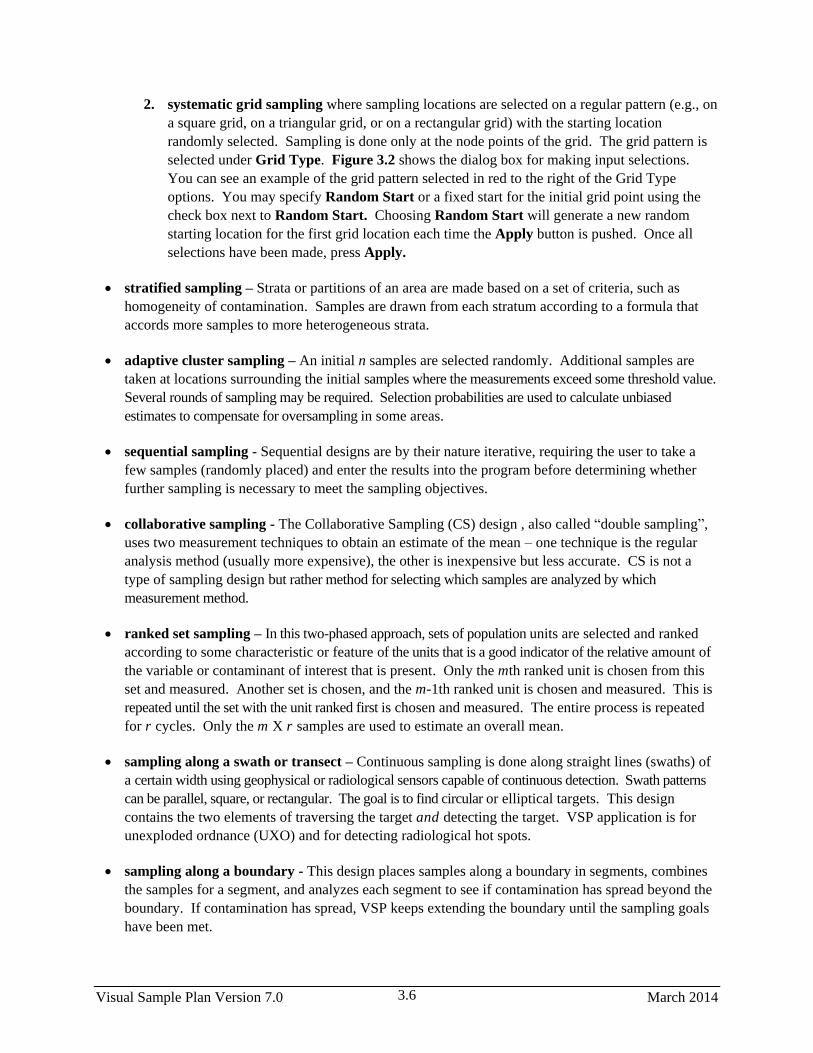
Visual Sample Plan Version 7.0 March 2014 3.6
2. systematic grid sampling where sampling locations are selected on a regular pattern (e.g., on
a square grid, on a triangular grid, or on a rectangular grid) with the starting location
randomly selected. Sampling is done only at the node points of the grid. The grid pattern is
selected under Grid Type. Figure 3.2 shows the dialog box for making input selections.
You can see an example of the grid pattern selected in red to the right of the Grid Type
options. You may specify Random Start or a fixed start for the initial grid point using the
check box next to Random Start. Choosing Random Start will generate a new random
starting location for the first grid location each time the Apply button is pushed. Once all
selections have been made, press Apply.
stratified sampling – Strata or partitions of an area are made based on a set of criteria, such as
homogeneity of contamination. Samples are drawn from each stratum according to a formula that
accords more samples to more heterogeneous strata.
adaptive cluster sampling – An initial n samples are selected randomly. Additional samples are
taken at locations surrounding the initial samples where the measurements exceed some threshold value.
Several rounds of sampling may be required. Selection probabilities are used to calculate unbiased
estimates to compensate for oversampling in some areas.
sequential sampling - Sequential designs are by their nature iterative, requiring the user to take a
few samples (randomly placed) and enter the results into the program before determining whether
further sampling is necessary to meet the sampling objectives.
collaborative sampling - The Collaborative Sampling (CS) design , also called “double sampling”,
uses two measurement techniques to obtain an estimate of the mean – one technique is the regular
analysis method (usually more expensive), the other is inexpensive but less accurate. CS is not a
type of sampling design but rather method for selecting which samples are analyzed by which
measurement method.
ranked set sampling – In this two-phased approach, sets of population units are selected and ranked
according to some characteristic or feature of the units that is a good indicator of the relative amount of
the variable or contaminant of interest that is present. Only the mth ranked unit is chosen from this
set and measured. Another set is chosen, and the m-1th ranked unit is chosen and measured. This is
repeated until the set with the unit ranked first is chosen and measured. The entire process is repeated
for r cycles. Only the m X r samples are used to estimate an overall mean.
sampling along a swath or transect – Continuous sampling is done along straight lines (swaths) of
a certain width using geophysical or radiological sensors capable of continuous detection. Swath patterns
can be parallel, square, or rectangular. The goal is to find circular or elliptical targets. This design
contains the two elements of traversing the target and detecting the target. VSP application is for
unexploded ordnance (UXO) and for detecting radiological hot spots.
sampling along a boundary - This design places samples along a boundary in segments, combines
the samples for a segment, and analyzes each segment to see if contamination has spread beyond the
boundary. If contamination has spread, VSP keeps extending the boundary until the sampling goals
have been met.

March 2014 Visual Sample Plan Version 7.0 3.7
multiple increment sampling – This design often arises because of the expense associated with
analytical tests. A researcher would randomly take n increments and combine them together into r
groups for analysis.
judgment sampling – You simply point and click anywhere in a sampling area. These sampling
locations are based on the judgment of the user.
Because judgment sampling is not probability-based, users can bias the sampling results
using this method. There is no basis in statistical theory for making confidence statements
about conclusions drawn when samples are selected by judgment. However, some problem
definitions might call for judgment sampling, such as looking in the most likely spot for
evidence of contamination or taking samples at predefined locations. Figure 3.3 shows
judgment sampling selected in VSP and six sampling locations selected manually.
Figure 3.3. Judgment Sampling in VSP

Visual Sample Plan Version 7.0 March 2014 3.8
3.2 DQO Inputs and Sample Size
The inputs needed for VSP’s sample-size calculations are decided upon during the DQO process. If you have
not gone through the DQO process prior to entering this information, you can enter “best guess” values for
each of the inputs and observe the resulting computed sample size. New inputs can be tried until a sample
size that is feasible and/or within budget is obtained. This iterative method for using VSP is a valuable
“what if” tool with which you can see the effect on sample size (and hence costs) of changing DQO
inputs. However, be cautioned that all the DQO elements interact and have special meaning within the
context of the problem. To be able to defend the sample size that VSP calculates, you must have a
defensible basis for each of the inputs. There is no quick way to generate this defense other than going
through Steps 1 through 6 of the DQO process.
The core set of DQO inputs that affect sample size for most of the designs are as follows:
Null Hypothesis Formulation – The null hypothesis is the working hypothesis or baseline condition
of the environment. There must be convincing evidence in the data to declare the baseline condition
to be false. VSP uses a default of “Site is Dirty” as the working hypothesis that must be disproved
with convincing evidence from the data.
Type I Error Rate (Alpha) – This is called the false rejection rate in EPA’s DQO guidance (EPA
2000a). This is the probability of rejecting a true null hypothesis. For the typical hypothesis test in
which we assume the survey unit is dirty (above the action level), alpha is the chance a dirty site with
a true mean equal to or greater than the Action Level will be released as clean to the public. In
general, alpha is the maximum chance, assuming the DQO inputs are true, that a dirty site will be
released as clean.
Type II Error Rate (Beta) – This is called the false acceptance rate in EPA’s DQO guidance. This is
the probability of not rejecting (accepting) a false null hypothesis. For the typical hypothesis test in
which we assume the survey unit is dirty, beta is the chance a specific clean site will be condemned as
dirty. Specifically, beta is the chance that a clean site with a true mean equal to or less than the
lower bound of the gray region will be condemned as dirty. In general, beta is the maximum chance,
outside the gray region, that a clean site will be condemned as dirty.
Width of Gray Region (Delta) – This is the distance from the Action Level to the outer bound of the
gray region. For the typical hypothesis test in which we assume the survey unit is dirty, the gray
region can be thought of as a range of true means where we are willing to decide that clean sites are
dirty with high probability. Typically, these probabilities are 20% to 95%, i.e., from beta to 1 -
alpha. If this region is reduced to a very small range, the sample size grows to be extremely large.
Determining a reasonable value for the size of the gray region calls for professional judgment and
cost/benefit evaluation.
Estimated Sampling Standard Deviation – This is an estimate of the standard deviation expected
between the multiple samples. This estimate could be obtained from previous studies, previous
experience with similar sites and contaminants, or expert opinion. Note that this is the square root of the
variance. In one form or another, all the designs require some type of user-input as to the variability
of contamination expected in the study area. After all, if the area to be sampled was totally
homogeneous, only one sample would be required to completely characterize the area.

March 2014 Visual Sample Plan Version 7.0 3.9
Other inputs are required by some of the designs, and other inputs are required for design parameters
other than sample size. For example, the stratified designs require the user to specify the desired number of
strata and estimates of proportions or standard deviations for each of the stratum. The UXO (unexploded
ordinance) modules use Bayesian methods and require the user to input their belief that the study area contains
UXO. When simulations are used, as in the post-survey UXO target detection, the user must input
assumptions about the distribution of scrap or shrapnel in the target areas. In the discussions of the designs, we
try to give an explanation of each input required of the user. If you are lost, use the VSP Help functions (See
Section 2.7).
Note: The Help Topics function in VSP provides a description of each of the designs and its related
inputs. You can also select the Help button on the toolbar, put the cursor on any of the designs on the
menu and a description of the design and its inputs will appear in a Help window. In addition, pressing
the Help button at the bottom of each design dialog will bring up a Help window that contains a complete
explanation of the design. Finally, on each screen where input is required, highlight an item and press the
F1 key for a description of that input item.
The next section contains a discussion of the inputs required by most of the designs available in the current
release of VSP. The designs are organized by the Sampling Goal under which they fall. Not all options
for all designs are discussed. Common design features (such as Costs, Historical Samples, MQO) that are
found in multiple designs will not be discussed individually in this section but can be found in
Section 5.0, Extended Features of VSP.
3.2.1 Compare Average to a Fixed Threshold
Comparing the average to a fixed threshold is the most common problem confronted by environmental
remediation engineers. We present different forms the problem might take and discuss how VSP can be
used to address each problem formulation.
We can continue where we left off in Section 2.3.3 with the Millsite.dxf map loaded. We selected a
single Sample Area from the site. The Action Level for the contaminant of interest is 6 pCi/g in the top 6 in.
of soil. Previous investigations indicate an estimated standard deviation of 2 pCi/g for the contaminant of
interest. The null hypothesis for this problem is “Assume Site is Dirty” or HO: True mean ≥ A.L.
We desire an alpha error rate of 1% and a beta error rate of 1%. According to EPA (2000a, pp. 6-10),
1% for both alpha and beta are the most stringent limits on decision errors typically encountered for
environmental data. We tentatively decide to set the lower bound of the gray region at 5 pCi/g and decide
a systematic grid is preferable.
We will use VSP to determine the final width of the gray region and the number of samples required.
Assume the fixed cost of planning and validation is $1,000, the field collection cost per sample is $100, and
the laboratory analytical cost per sample is $400. We are told to plan on a maximum sampling budget of
$20,000.
Case 1: We assume that the population from which we are sampling is approximately normal or that it is
well-behaved enough that the Central Limit Theorem of statistics applies. In other words, the distribution
of sample means drawn from the population is approximately normally distributed. We also decided that
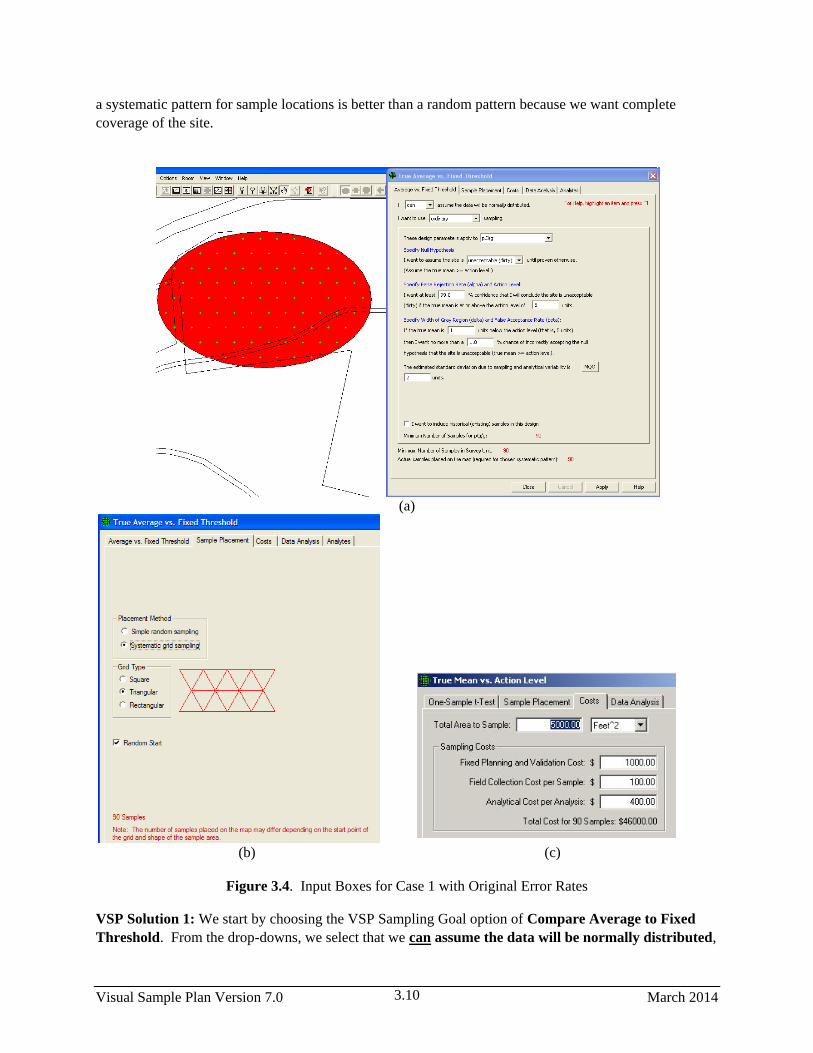
Visual Sample Plan Version 7.0 March 2014 3.10
a systematic pattern for sample locations is better than a random pattern because we want complete
coverage of the site.
(a)
(b) (c)
Figure 3.4. Input Boxes for Case 1 with Original Error Rates
VSP Solution 1: We start by choosing the VSP Sampling Goal option of Compare Average to Fixed
Threshold. From the drop-downs, we select that we can assume the data will be normally distributed,

March 2014 Visual Sample Plan Version 7.0 3.11
and that we want to use ordinary sampling. For Sample Placement, we select Systematic grid sampling.
For Grid Type we select Triangular with a Random Start. A grouping of the input dialogs is shown in
Figure 3.4. Note that instead of inputting the alpha error rate directly, it is input as the confidence (100%
- alpha%) in correctly accepting the null hypothesis.
We see that for our inputs, using a one-sample t-test will require taking 90 samples at a cost of $46,000.
Clearly, we need to relax our error tolerances or request more funding.
For the sake of argument, suppose all the stakeholders agree that an alpha error rate of 5% and a beta
error rate of 10% are acceptable. Figure 3.5 reveals that those changes lead to a significant reduction in
the sampling cost, now $19,000 for n = 36 samples.
Are these new error rates justifiable? Only the specific context of each problem and the professional judgment
of those involved can answer that question. What about the assumption that we will be able to use a parametric
test, the one-sample t-test? Unless the population from which we are sampling is quite skewed, our new
Figure 3.5. Input Boxes for Case 1 with Increased Error Rates
sample size of n = 36 is probably large enough to justify using a parametric test. Of course, once we take
the data, we will need to justify our assumptions as pointed out in Guidance for Data Quality Assessment
Practical Methods for Data Analysis (EPA 2000b, pp. 3-5).
Case 2: We now decide that we want to look at designs that may offer us cost savings over the
systematic design just presented. We have methods available for collecting and analyzing samples in the
field making quick turnaround possible. We want to be efficient and cost-effective and take only enough

Visual Sample Plan Version 7.0 March 2014 3.12
samples to confidently say whether our site is clean or dirty. After all, if our first several samples exhibit
levels of contamination so high that there is no possible scenario for the average to be less than a
threshold, why continue to take more samples? We can make a decision right now that the site needs to be
remediated. Sequential designs, and the tests associated with them, take previous sampling results into
account and provide rules specifying when sampling can stop and a decision can be made.
VSP Solution 2a: From VSP’s main menu, select the Sampling Goal of Compare Average to a Fixed
Threshold. From the drop-downs, select that we can assume the data will be normally distributed,
and that we want to use sequential sampling. The dialog box in Figure 3.6 appears. We begin by
entering the DQO parameters for Alpha, Beta, Action Level, etc., which in Figure 3.6 are shown in a
sentence structure format. Next, enter the Number of Samples Per Round, shown here as 3. This
parameter indicates how many samples you want to take each time you mobilize into the field. Each time
you press the Apply button, VSP places a pattern of this many sampling locations on the map, except for
the first round where at least 10 samples are needed to get an estimate of the standard deviation.
Figure 3.6. Dialog for Sequential Sampling (Standard Deviation Known) and Ten Locations Placed
on the Map
In Figure 3.6, we see the results of pressing Apply. Ten locations are placed on the Map labeled “Seq-001,
Seq-002, etc.”

March 2014 Visual Sample Plan Version 7.0 3.13
Once the sample results are available, click on the Data Analysis tab, go to the Data Entry sub-page, and
enter the measurement values for those ten samples into the grid on the data input dialog. We enter these
values as 5, 8, 6, 7, 5, 4, 8, 4, 7 and 5. Press the Apply button and in VSP you will see that three more
samples have been generated. Return to the Average vs. Fixed Threshold tab. We now see in Figure
3.7 that the Number of Samples Collected as 10, and that VSP cannot accept or reject the null
hypothesis on the basis of these samples and suggests that up to 2 additional samples may be needed to
make a decision. (Note that VSP will not accept or reject the null hypothesis with fewer than 10
samples). VSP asks you to take 3 more samples, which are the three new samples placed on the map.
Figure 3.7. Data Input Dialog for Sequential Probability Ratio Test and Results from First Round of
Sampling. Map View is shown in background.
Switching over to the Graph View in Figure 3.8, we can see that in order to accept the null hypothesis that
the site is dirty we need to take more than 10 samples. The open circles show the test statistic as the data
are collected. The last 3 samples that appear on the graph are the next three samples, which can be
entered in the Data Analysis tab’s Data Entry sub-page as 6, 7, and 8. VSP now tells us that we can
Accept the Null Hypothesis and conclude the site is dirty.

Visual Sample Plan Version 7.0 March 2014 3.14
Figure 3.8. Graph View of Sequential Sampling
VSP Solution 2b. We have one other option for more cost-efficient sampling – reduce the analytic
laboratory costs by taking advantage of measurement equipment that may be less accurate, but is less
expensive. (Note that the two methods do not even have to measure the same thing as long as there is a
linear correlation between them. For example, the expensive method may measure the concentration of
Plutonium metal in soil and the inexpensive method may measure low-energy gamma radiation emitted
by Americium in soil. This works because Americium is a daughter product of Plutonium decay). If we
can still meet our DQOs (error levels, width of grey region) taking advantage of the less expensive
equipment, we will save money.
It works like this: At ‘n’ field locations selected using simple random sampling or grid sampling, the
inexpensive analysis method is used. Then, for some of the ‘n’ locations, the expensive analysis method
is also conducted (nE). The data from these two analysis methods are used to estimate the mean and the
standard error (SE: the standard deviation of the estimated mean). The method of estimating the mean
and SE assumes there is a linear relationship between the inexpensive and expensive analysis methods. If
the linear correlation between the two methods is sufficiently high (close to 1), and if the cost of the
inexpensive analysis method is sufficiently less than that of the expensive analysis method, then
Collaborative Sampling (CS) is expected to be more cost effective at estimating the population mean than
if the entire measurement budget was spent on obtaining only expensive analysis results at field locations
selected using simple random sampling or grid sampling.

March 2014 Visual Sample Plan Version 7.0 3.15
If Collaborative Sampling is chosen for the Sampling Goal of Compare Average to a Fixed Threshold
the resulting Map View of the applied CS samples on the Millsite.dxf map are all shown in Figure 3.9.
Figure 3.9. Dialog Box for Collaborative Sampling and Map View of Applied CS Samples
The first set of inputs requested in the Data Input Dialog Box for CS are those needed to determine
whether CS sampling is more cost effective than using only expensive measurements and simple random
sampling. The first input required is the correlation coefficient between expensive and inexpensive
measurements computed on the same set of samples. This is determined from data in prior studies or in a
pilot study. The next two inputs are the cost estimates: the cost per unit of making a single expensive
measurement, including the cost of sample collection, handling, preparation and measurement; and the
cost per unit of making a single inexpensive measurement, including finding the field location and
conducting the inexpensive analysis method.
The next set of inputs comprises the DQOs for the problem. Notice that these are the same inputs we
used for Case 1 with increased error rates (see Figure 3.5) when VSP calculated a required sample size of
36. If all those 36 samples were analyzed with the expensive method, the total cost would be 36 x $400 =
$14,400. However, if we use CS and the same DQOs, VSP calculates we need to take 66 samples
measured by the inexpensive method, and 23 of those 66 samples measured by the expensive method.
This costs a total of 66 x $60 = 3960 plus 23 x $400 = $9200 for a total of $13,160. This represents a
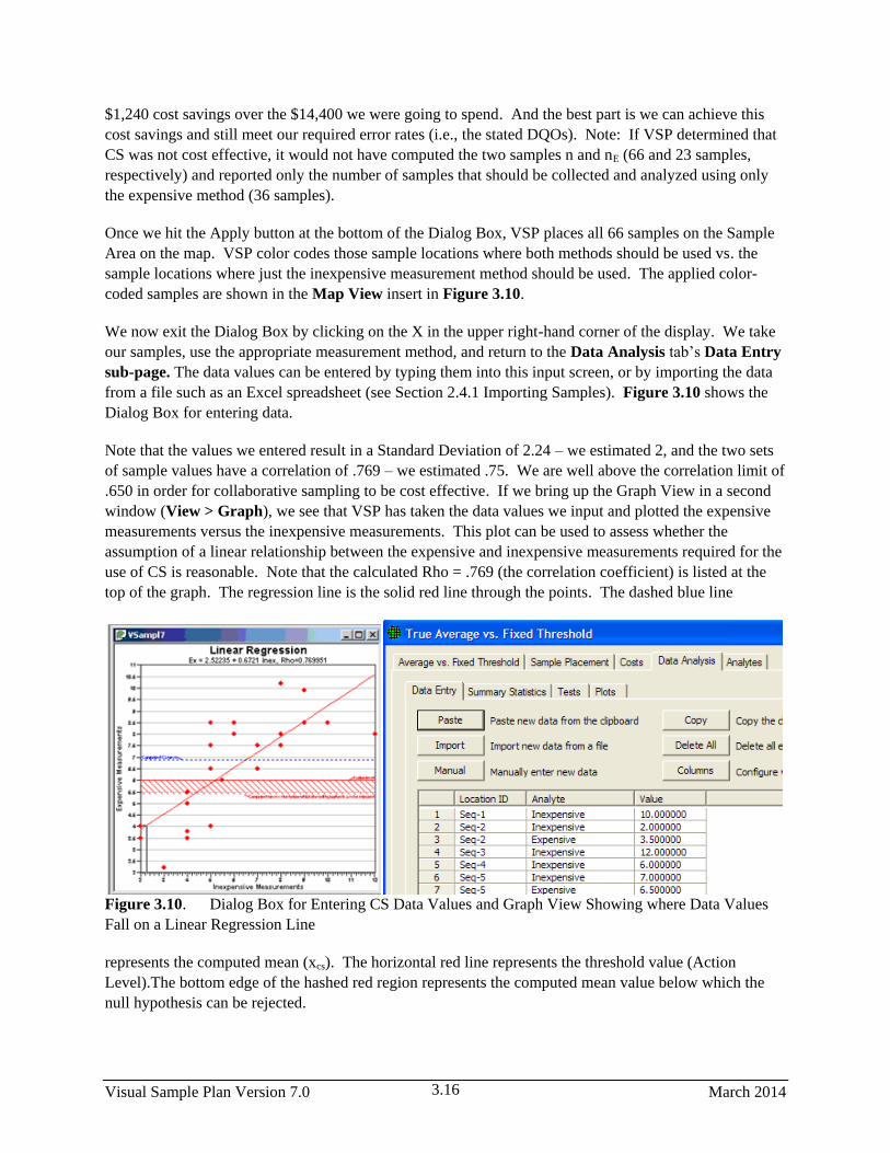
Visual Sample Plan Version 7.0 March 2014 3.16
$1,240 cost savings over the $14,400 we were going to spend. And the best part is we can achieve this
cost savings and still meet our required error rates (i.e., the stated DQOs). Note: If VSP determined that
CS was not cost effective, it would not have computed the two samples n and nE (66 and 23 samples,
respectively) and reported only the number of samples that should be collected and analyzed using only
the expensive method (36 samples).
Once we hit the Apply button at the bottom of the Dialog Box, VSP places all 66 samples on the Sample
Area on the map. VSP color codes those sample locations where both methods should be used vs. the
sample locations where just the inexpensive measurement method should be used. The applied color-
coded samples are shown in the Map View insert in Figure 3.10.
We now exit the Dialog Box by clicking on the X in the upper right-hand corner of the display. We take
our samples, use the appropriate measurement method, and return to the Data Analysis tab’s Data Entry
sub-page. The data values can be entered by typing them into this input screen, or by importing the data
from a file such as an Excel spreadsheet (see Section 2.4.1 Importing Samples). Figure 3.10 shows the
Dialog Box for entering data.
Note that the values we entered result in a Standard Deviation of 2.24 – we estimated 2, and the two sets
of sample values have a correlation of .769 – we estimated .75. We are well above the correlation limit of
.650 in order for collaborative sampling to be cost effective. If we bring up the Graph View in a second
window (View > Graph), we see that VSP has taken the data values we input and plotted the expensive
measurements versus the inexpensive measurements. This plot can be used to assess whether the
assumption of a linear relationship between the expensive and inexpensive measurements required for the
use of CS is reasonable. Note that the calculated Rho = .769 (the correlation coefficient) is listed at the
top of the graph. The regression line is the solid red line through the points. The dashed blue line
Figure 3.10. Dialog Box for Entering CS Data Values and Graph View Showing where Data Values
Fall on a Linear Regression Line
represents the computed mean (xcs). The horizontal red line represents the threshold value (Action
Level).The bottom edge of the hashed red region represents the computed mean value below which the
null hypothesis can be rejected.

March 2014 Visual Sample Plan Version 7.0 3.17
VSP reports that based on the data values input, we can Accept the Null Hypothesis: Assume the Site is
Dirty.
If we had chosen Simple Random Sampling rather than Systematic Grid Sampling on the Sample
Placement tab, all the sample sizes would have been the same. The only difference would have been that
the samples would have been placed on the Map in a grid pattern rather than randomly.
Case 3: We do not wish to assume that the population from which we are sampling is approximately
normal.
VSP Solution 3a: The purpose of a MARSSIM sign test is to test a hypothesis involving the true mean
or median of a population against an Action Level. Using this test for the mean assumes the distribution
of the target population is symmetrical. When the distribution of the target population is symmetrical, the
mean and the median are the same. When the distribution is not symmetrical, the Sign test is a true test
for the median, and an approximate test for the mean. The appropriate use of the Sign Test for final status
surveys is discussed in Multi-Agency Radiation Survey and Site Investigation Manual (MARSSIM) (EPA
1997). This document is currently available at http://www.epa.gov/radiation/marssim/. The input for
the MARSSIM Sign Test is shown in Figure 3.11.
Figure 3.11. Dialog Box for the MARSSIM Sign Test
VSP Solution 3b: From VSP’s main menu, select the Sampling Goal of Compare Average to a Fixed
Threshold. From the drop-downs, select that we cannot assume the data will be normally distributed,
and that our data are symmetrical (the mean and median are the same). Note that using this test for
the mean assumes the distribution of the target population is symmetrical. A grouping of the input
dialogs is shown in Figure 3.12.

Visual Sample Plan Version 7.0 March 2014 3.18
Figure 3.12. Input Dialog for Wilcoxon Signed Rank Test
For our inputs, and assuming that we will use a nonparametric Wilcoxon Signed Ranks test to analyze our
data, VSP indicates that we are required to take 42 samples at a cost of $22,000. This is $3,000 more than
the previous parametric case, given the same input parameters. Is the choice of a nonparametric test
worth the extra $3,000 in sampling costs beyond what was required for the parametric one-sample t-test?
VSP does not address that kind of question. Professional judgment is needed. You must make the
decision based on the best available data, the consequences of decision errors, and legal and ethical

March 2014 Visual Sample Plan Version 7.0 3.19
considerations. If little pre-existing information is available, a pilot study to gain a better understanding of
the characteristics of the population may be indicated, since a symmetric distribution of the target
population is assumed.
3.2.2 Compare Average to Reference Average
We again start with the Millsite.dxf map from Section 2.3.3 with a single Sample Area defined. The
Action Level for the contaminant of interest is 5 pCi/g above background in the top 6 in. of soil. Background
is found by sampling an appropriate reference area. Previous investigations indicate an estimated
standard deviation of 2 pCi/g for the contaminant of interest. The null hypothesis for this problem is
“Assume Site is Dirty” or HO: Difference of True Means ≥ Action Level. In other words, the parameter
of interest for this test is the difference of means, not an individual mean as was the case in the one-
sample t-test.
We desire an alpha error rate of 1% and a beta error rate of 1%. We tentatively decide to set the lower
bound of the gray region to 4 pCi/g above background, i.e., a difference of means of 4 pCi/g. Using VSP,
we will determine the final width of the gray region and the number of samples required.
Assume that the fixed planning and validation cost is $1,000, the field collection and measurement cost per
sample is $100, and the laboratory analytical cost per sample is $0 because we are able to justify the use
of field measurements. We are told to plan on a maximum sampling budget of $20,000 for both the
Reference Area and the Study Area.
Case 4: We assume that the populations we are sampling are approximately normal or that they are well--
behaved enough so that the Central Limit Theorem of statistics applies. In other words, the distributions of
sample means drawn from the two populations are approximately normally distributed. If that is the case,
the distribution of the differences also will be approximately normally distributed. We also assume the
standard deviations of both populations are approximately equal. In addition, we determine that a systematic
grid sampling scheme is preferable.
VSP Solution 4a: We start by choosing from the main menu: Sampling Goals > Compare Average to
Reference Average. A grouping of the input dialogs is shown in Figure 3.13.
Visual Sample Plan Version 7.0 March 2014 3.20
Figure 3.13. Input Dialogs for Case 4 with Original Error Rates
We see that for our inputs, using a two-sample t-test will require taking 175 field samples in the Sample
Area at a cost of $18,500. The sampling cost for the Reference Area also will be $17,500 (assuming the
fixed costs will not be incurred a second time). The combined sampling cost of $36,000 is significantly
beyond our budget of $20,000. What will be the result if we relax the error rates somewhat?
In Figure 3.14, by increasing both the alpha error rate and the beta error rate to 5%, the sampling cost for
one area has decreased to $9,800 based on n = 88 field samples. Thus, the new combined cost of $18,600
achieves our goal of no more than $20,000.
Can we justify these larger error rates? Again, only professional judgment using the best information
related to the current problem can answer that question.
What about our planned use of a parametric test, the two-sample t-test? A sample size of 88 is large
enough that we can probably safely assume the two-sample t-test will meet the assumption of normality
for the differences of sample means. We should test this assumption after the data are collected.
What about the assumption of approximately equal standard deviations for the measurements in the
Sample and Reference Areas? When we collect the data, we will need to check that assumption. See
Guidance for Data Quality Assessment Practical Methods for Data Analysis (EPA 2000b, pp. 3-26) for
the use of Satterthwaite’s t-test when the standard deviations (or variances) of the two areas are not
approximately equal.
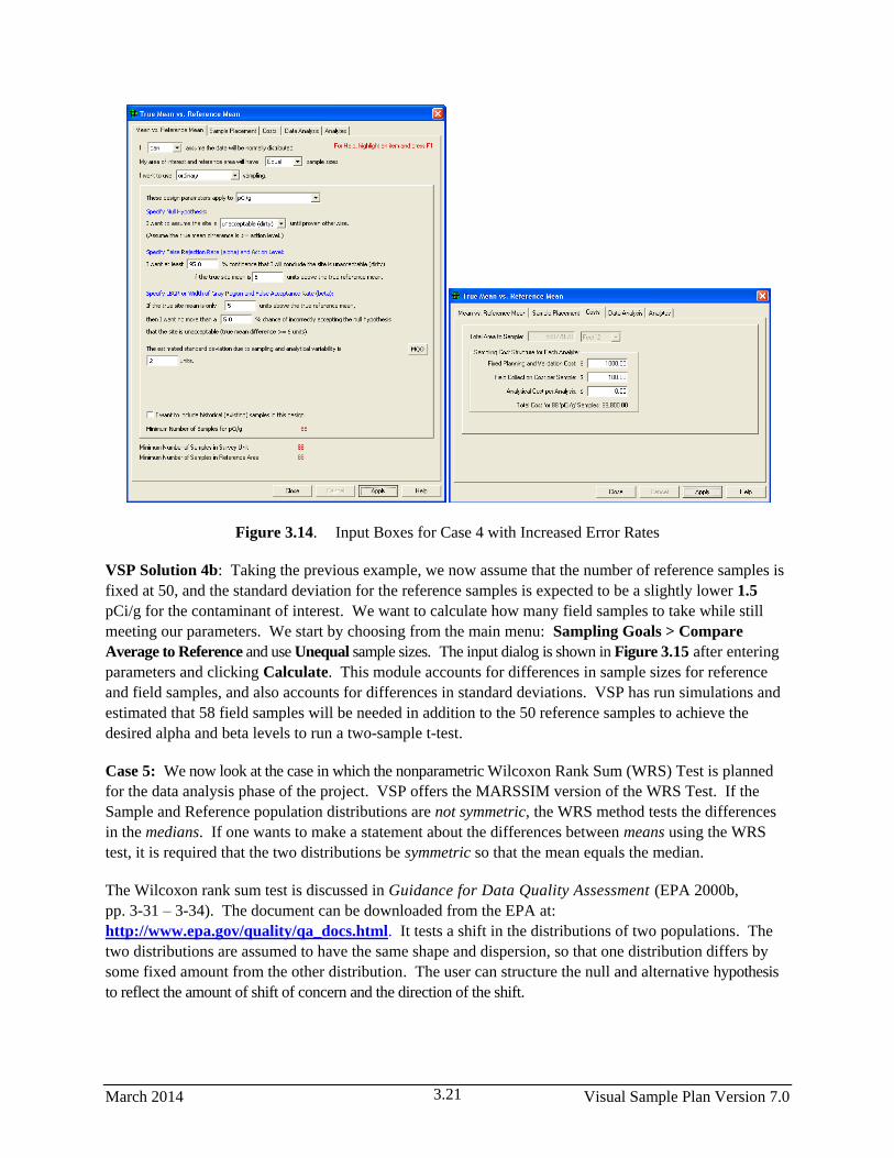
March 2014 Visual Sample Plan Version 7.0 3.21
Figure 3.14. Input Boxes for Case 4 with Increased Error Rates
VSP Solution 4b: Taking the previous example, we now assume that the number of reference samples is
fixed at 50, and the standard deviation for the reference samples is expected to be a slightly lower 1.5
pCi/g for the contaminant of interest. We want to calculate how many field samples to take while still
meeting our parameters. We start by choosing from the main menu: Sampling Goals > Compare
Average to Reference and use Unequal sample sizes. The input dialog is shown in Figure 3.15 after entering
parameters and clicking Calculate. This module accounts for differences in sample sizes for reference
and field samples, and also accounts for differences in standard deviations. VSP has run simulations and
estimated that 58 field samples will be needed in addition to the 50 reference samples to achieve the
desired alpha and beta levels to run a two-sample t-test.
Case 5: We now look at the case in which the nonparametric Wilcoxon Rank Sum (WRS) Test is planned
for the data analysis phase of the project. VSP offers the MARSSIM version of the WRS Test. If the
Sample and Reference population distributions are not symmetric, the WRS method tests the differences
in the medians. If one wants to make a statement about the differences between means using the WRS
test, it is required that the two distributions be symmetric so that the mean equals the median.
The Wilcoxon rank sum test is discussed in Guidance for Data Quality Assessment (EPA 2000b,
pp. 3-31 – 3-34). The document can be downloaded from the EPA at:
http://www.epa.gov/quality/qa_docs.html. It tests a shift in the distributions of two populations. The
two distributions are assumed to have the same shape and dispersion, so that one distribution differs by
some fixed amount from the other distribution. The user can structure the null and alternative hypothesis
to reflect the amount of shift of concern and the direction of the shift.

Visual Sample Plan Version 7.0 March 2014 3.22
Figure 3.15 Input Dialog for Case 4 with Unequal Sample Sizes and Unequal Standard Deviations
VSP Solution 5: We start by choosing from VSP’s main menu Sampling Goals > Compare Average to
Reference Average and select that you cannot assume the data are normally distributed. A grouping of the input
dialogs is shown in Figure 3.16.
Shown in Figure 3.16, the input dialog for the MARSSIM WRS test allows the user to supply a percent
overage to apply to the sample size calculation. MARSSIM suggests that the number of samples should be
increased by at least 20% to account for missing or unusable data and for uncertainty in the calculated values
of Sample Size, (EPA 1997, p. 5-29). With the extra 20%, 114 samples are required in both the Sample
Area (i.e., Survey Unit or Study Area) and Reference Area.
The cost per area is now $12,400. The larger sample size of 114 instead of the previous sample size of 88 is
probably not justified. However, professional judgment is needed to make the final decision.

March 2014 Visual Sample Plan Version 7.0 3.23
Figure 3.16. Input Boxes for Case 5 Using Nonparametric Wilcoxon Rank Sum Test
The MARSSIM WRS test is used to test whether the true median in a Survey Unit population is greater
than the true median in a Reference Area population. The test compares medians of the two populations
because the WRS is based on ranks rather than the measurements themselves. Note that if both the
Survey Unit and Reference Area populations are symmetric, then the median and mean of each
distribution are identical. In that special case the MARSSIM WRS test is comparing means. The
assumption of symmetry and the appropriate use of the WRS test for final status surveys is discussed in
Multi-Agency Radiation Survey and Site Investigation Manual (MARSSIM) (EPA 2000). This document
is currently available at: http://www.epa.gov/radiation/marssim/.
Case 6: Next, assume that the population from which we will be sampling is non-normal but symmetric
and we again desire to use a nonparametric Wilcoxon rank sum test. However, we are limited to a total
sampling budget for both areas of $10,000. By using VSP iteratively, we will adjust the various DQO
input parameters and try to discover a sampling plan that will meet the new goals.
VSP Solution 6: Figure 3.17 shows that with an alpha of 5%, a beta of 12.5%, and a lower bound of the
gray region of 3.5, the number of samples per area drops to 39. With a sampling cost of $3,900 for each
sampling area, and assuming the fixed costs of $1,000 will only occur once, we now have a combined cost of
$8,800 and thus meet our goal of $10,000.

Visual Sample Plan Version 7.0 March 2014 3.24
Figure 3.17. Input Boxes for Case 6 Using Nonparametric Wilcoxon Rank Sum Test
Will relaxing the error tolerances and increasing the width of the gray region to meet the requirements of the
smaller sampling budget be acceptable to all stakeholders in the DQO process? Again, it depends on the
objectives and judgment of those involved in the process.
Case 7: Suppose our combined sampling budget is reduced to $5,000. Can VSP provide a sampling design
that meets that goal?
VSP Solution 7: Figure 3.18 shows a design with just 15 samples per sampling area that meets the new
sparse budget. We reduced the combined sampling cost, now $5,000, by increasing the width of the gray
region to 2.35 pCi/g (lower bound of the gray region is 2.65 pCi/g) and by increasing the beta level to 0.20
(20%).
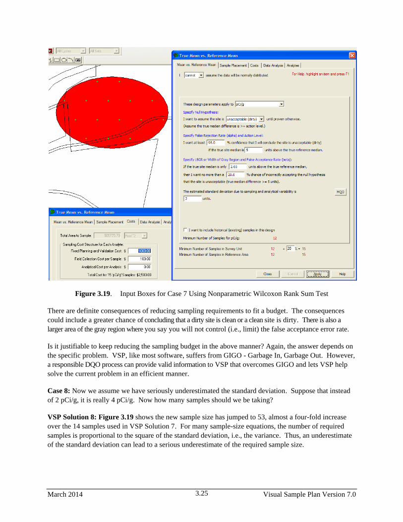
March 2014 Visual Sample Plan Version 7.0 3.25
Figure 3.19. Input Boxes for Case 7 Using Nonparametric Wilcoxon Rank Sum Test
There are definite consequences of reducing sampling requirements to fit a budget. The consequences
could include a greater chance of concluding that a dirty site is clean or a clean site is dirty. There is also a
larger area of the gray region where you say you will not control (i.e., limit) the false acceptance error rate.
Is it justifiable to keep reducing the sampling budget in the above manner? Again, the answer depends on
the specific problem. VSP, like most software, suffers from GIGO - Garbage In, Garbage Out. However,
a responsible DQO process can provide valid information to VSP that overcomes GIGO and lets VSP help
solve the current problem in an efficient manner.
Case 8: Now we assume we have seriously underestimated the standard deviation. Suppose that instead
of 2 pCi/g, it is really 4 pCi/g. Now how many samples should we be taking?
VSP Solution 8: Figure 3.19 shows the new sample size has jumped to 53, almost a four-fold increase
over the 14 samples used in VSP Solution 7. For many sample-size equations, the number of required
samples is proportional to the square of the standard deviation, i.e., the variance. Thus, an underestimate
of the standard deviation can lead to a serious underestimate of the required sample size.
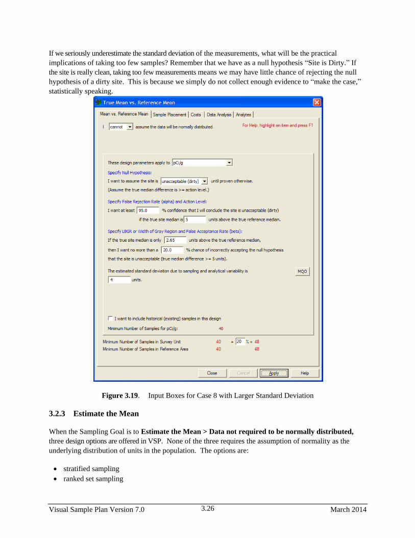
Visual Sample Plan Version 7.0 March 2014 3.26
If we seriously underestimate the standard deviation of the measurements, what will be the practical
implications of taking too few samples? Remember that we have as a null hypothesis “Site is Dirty.” If
the site is really clean, taking too few measurements means we may have little chance of rejecting the null
hypothesis of a dirty site. This is because we simply do not collect enough evidence to “make the case,”
statistically speaking.
Figure 3.19. Input Boxes for Case 8 with Larger Standard Deviation
3.2.3 Estimate the Mean
When the Sampling Goal is to Estimate the Mean > Data not required to be normally distributed,
three design options are offered in VSP. None of the three requires the assumption of normality as the
underlying distribution of units in the population. The options are:
stratified sampling
ranked set sampling
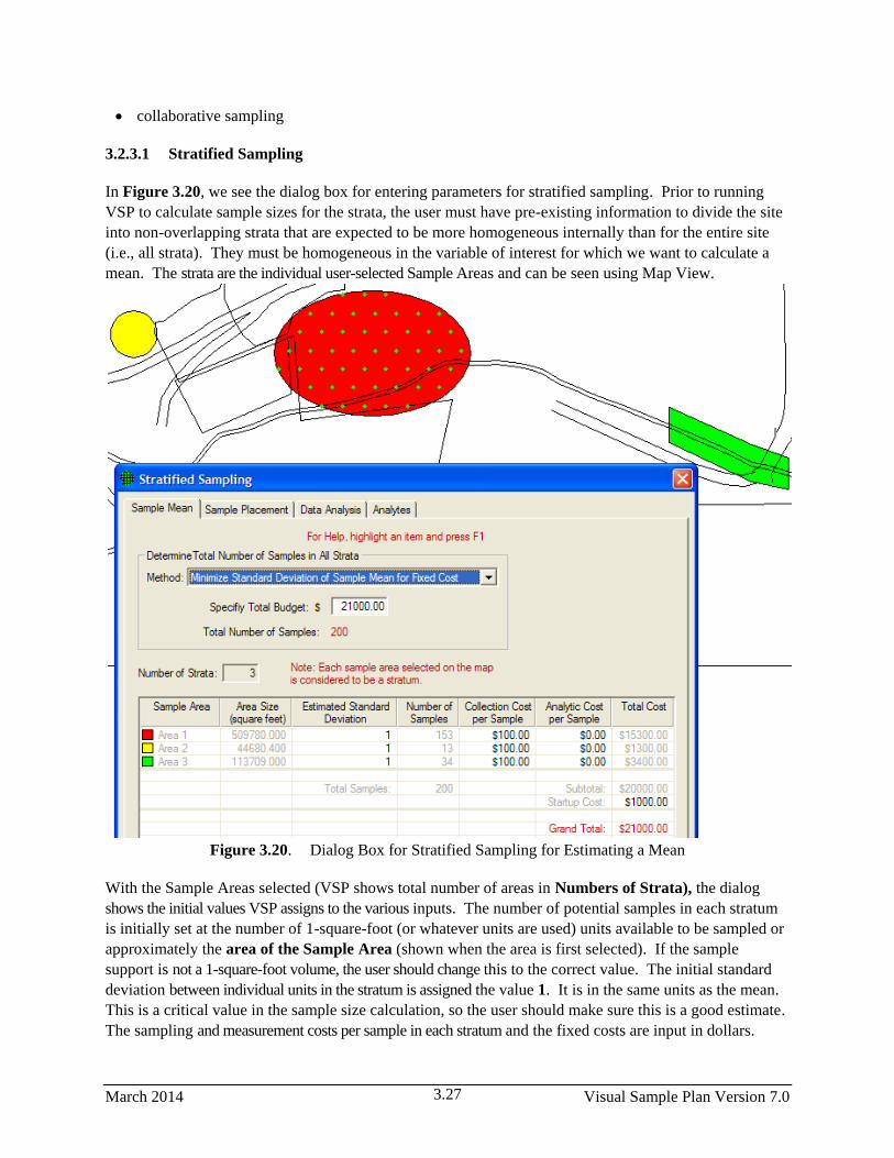
March 2014 Visual Sample Plan Version 7.0 3.27
collaborative sampling
3.2.3.1 Stratified Sampling
In Figure 3.20, we see the dialog box for entering parameters for stratified sampling. Prior to running
VSP to calculate sample sizes for the strata, the user must have pre-existing information to divide the site
into non-overlapping strata that are expected to be more homogeneous internally than for the entire site
(i.e., all strata). They must be homogeneous in the variable of interest for which we want to calculate a
mean. The strata are the individual user-selected Sample Areas and can be seen using Map View.
Figure 3.20. Dialog Box for Stratified Sampling for Estimating a Mean
With the Sample Areas selected (VSP shows total number of areas in Numbers of Strata), the dialog
shows the initial values VSP assigns to the various inputs. The number of potential samples in each stratum
is initially set at the number of 1-square-foot (or whatever units are used) units available to be sampled or
approximately the area of the Sample Area (shown when the area is first selected). If the sample
support is not a 1-square-foot volume, the user should change this to the correct value. The initial standard
deviation between individual units in the stratum is assigned the value 1. It is in the same units as the mean.
This is a critical value in the sample size calculation, so the user should make sure this is a good estimate.
The sampling and measurement costs per sample in each stratum and the fixed costs are input in dollars.
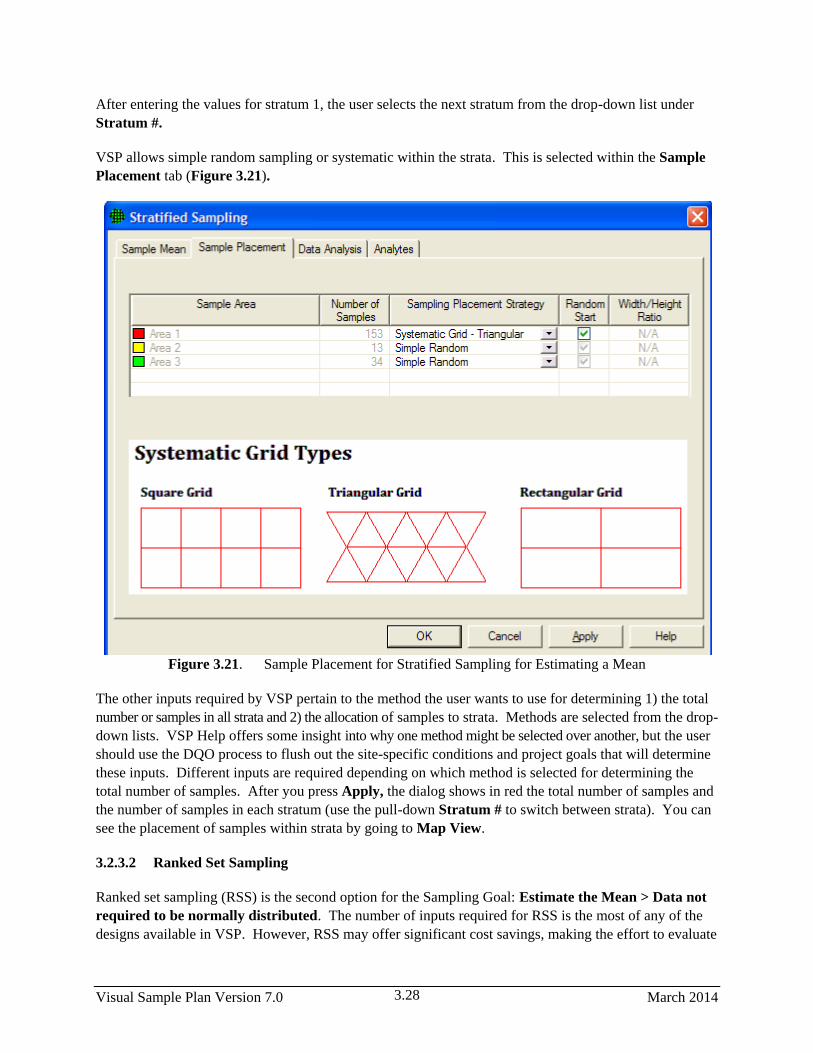
Visual Sample Plan Version 7.0 March 2014 3.28
After entering the values for stratum 1, the user selects the next stratum from the drop-down list under
Stratum #.
VSP allows simple random sampling or systematic within the strata. This is selected within the Sample
Placement tab (Figure 3.21).
Figure 3.21. Sample Placement for Stratified Sampling for Estimating a Mean
The other inputs required by VSP pertain to the method the user wants to use for determining 1) the total
number or samples in all strata and 2) the allocation of samples to strata. Methods are selected from the drop-
down lists. VSP Help offers some insight into why one method might be selected over another, but the user
should use the DQO process to flush out the site-specific conditions and project goals that will determine
these inputs. Different inputs are required depending on which method is selected for determining the
total number of samples. After you press Apply, the dialog shows in red the total number of samples and
the number of samples in each stratum (use the pull-down Stratum # to switch between strata). You can
see the placement of samples within strata by going to Map View.
3.2.3.2 Ranked Set Sampling
Ranked set sampling (RSS) is the second option for the Sampling Goal: Estimate the Mean > Data not
required to be normally distributed. The number of inputs required for RSS is the most of any of the
designs available in VSP. However, RSS may offer significant cost savings, making the effort to evaluate
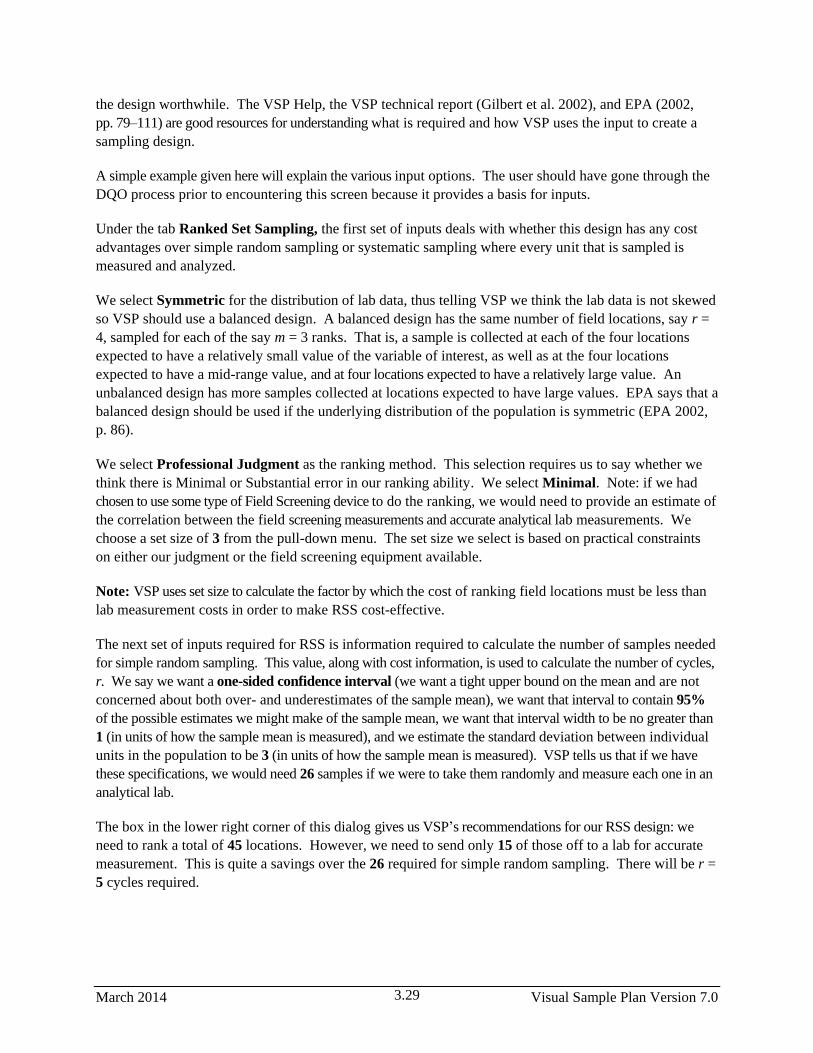
March 2014 Visual Sample Plan Version 7.0 3.29
the design worthwhile. The VSP Help, the VSP technical report (Gilbert et al. 2002), and EPA (2002,
pp. 79–111) are good resources for understanding what is required and how VSP uses the input to create a
sampling design.
A simple example given here will explain the various input options. The user should have gone through the
DQO process prior to encountering this screen because it provides a basis for inputs.
Under the tab Ranked Set Sampling, the first set of inputs deals with whether this design has any cost
advantages over simple random sampling or systematic sampling where every unit that is sampled is
measured and analyzed.
We select Symmetric for the distribution of lab data, thus telling VSP we think the lab data is not skewed
so VSP should use a balanced design. A balanced design has the same number of field locations, say r =
4, sampled for each of the say m = 3 ranks. That is, a sample is collected at each of the four locations
expected to have a relatively small value of the variable of interest, as well as at the four locations
expected to have a mid-range value, and at four locations expected to have a relatively large value. An
unbalanced design has more samples collected at locations expected to have large values. EPA says that a
balanced design should be used if the underlying distribution of the population is symmetric (EPA 2002,
p. 86).
We select Professional Judgment as the ranking method. This selection requires us to say whether we
think there is Minimal or Substantial error in our ranking ability. We select Minimal. Note: if we had
chosen to use some type of Field Screening device to do the ranking, we would need to provide an estimate of
the correlation between the field screening measurements and accurate analytical lab measurements. We
choose a set size of 3 from the pull-down menu. The set size we select is based on practical constraints
on either our judgment or the field screening equipment available.
Note: VSP uses set size to calculate the factor by which the cost of ranking field locations must be less than
lab measurement costs in order to make RSS cost-effective.
The next set of inputs required for RSS is information required to calculate the number of samples needed
for simple random sampling. This value, along with cost information, is used to calculate the number of cycles,
r. We say we want a one-sided confidence interval (we want a tight upper bound on the mean and are not
concerned about both over- and underestimates of the sample mean), we want that interval to contain 95%
of the possible estimates we might make of the sample mean, we want that interval width to be no greater than
1 (in units of how the sample mean is measured), and we estimate the standard deviation between individual
units in the population to be 3 (in units of how the sample mean is measured). VSP tells us that if we have
these specifications, we would need 26 samples if we were to take them randomly and measure each one in an
analytical lab.
The box in the lower right corner of this dialog gives us VSP’s recommendations for our RSS design: we
need to rank a total of 45 locations. However, we need to send only 15 of those off to a lab for accurate
measurement. This is quite a savings over the 26 required for simple random sampling. There will be r =
5 cycles required.

Visual Sample Plan Version 7.0 March 2014 3.30
Note: If we had chosen an unbalanced design, VSP would tell us how many times the top ranked location
needed to be sampled per cycle. Also, the inputs for the confidence interval would change slightly for the
unbalanced design.
All costs (fixed, field collection per sample, analytical cost for sending a sample to the lab, and ranking
cost per location) are entered on the dialog box that appears when the Cost tab is selected. In Figure
3.22, we see the two dialog boxes for RSS.
Once we press Apply, the RSS toolbar appears on our screen. The RSS toolbar lets us explore the
locations to be ranked and the locations to be sampled and measured under Map View. VSP produces
sample markers on the map that have different shapes and colors. The color of the marker indicates its cycle.
The cycle colors start at red and go through the spectrum to violet. Selecting one of the cycles on the pull-
down menu displays only the field locations for that cycle. In Figure 3.23, all the green field locations for
Cycle 3 are shown. The shape of the marker indicates its set. Field sample locations for the first set are
Figure 3.22. Dialog Boxes for Ranked Set Sampling Design
Figure 3.23. Map of RSS Field Sample Locations for All Sets in Cycle 3, Along with RSS Toolbar

March 2014 Visual Sample Plan Version 7.0 3.31
marked with squares, locations for the second set are marked with triangles, and so on. We show All Sets
in Figure 3.23. For unbalanced designs, the top set is sampled several times, so a number accompanies
those markers. Our example is for a balanced design so we do not see numbers.
Ranked set field sampling locations are generated with a label having the following format: RSS-c-s-i
where c = the cycle number
s = the set number (the unbalanced design for this number is also incremented for each iteration of
the top set)
I = a unique identifier within the set.
Use View > Labels > Labels on the
main menu or the AB button on the main
toolbar (button also on the RSS toolbar)
to show or hide the labels for the field
sample locations. Figure 3.24 shows the
labels on the map for field sample
locations associated with Cycle 3, All
Sets.
3.2.3.3 Collaborative Sampling for
Estimating the Mean
The third design we discuss for a cost-
effective option for estimating the mean
when normality cannot be assumed is
Collaborative Sampling (CS) –
sometimes called Double Sampling.
This design is applicable where two or
more techniques are available for measuring the amount of pollutant in an environmental sample, for
example a field method (inexpensive, less accurate) and a fixed lab method (expensive, more accurate).
The approach is to use both techniques on a small number of samples, and supplement this information
with a larger of number of samples measured only by the more expensive method. This approach will be
cost-effective if the linear correlation between measurements obtained by both techniques on the same
samples is sufficiently near 1 and if the less accurate method is substantially less costly than the more
accurate method
Collaborative Sampling works like this: At n field locations selected using simple random sampling or
grid sampling, the inexpensive analysis method is used. Then, for each of nE of the n locations, the
expensive analysis method is also conducted. The data from these two analysis methods are used to
estimate the mean and the standard error (SE: the standard deviation of the estimated mean). The method
of estimating the mean and SE assumes there is a linear relationship between the inexpensive and
expensive analysis methods.
VSP has an extensive discussion of CS in the Help. CS is also discussed in Gilbert (1987), Chapter 9,
where you can find an actual Case Study using CS. In Figure 3.25 we show the input screen for
Collaborative Sampling.
Figure 3.24. Map of RSS Field Sampling Locations Along
with Their Labels

Visual Sample Plan Version 7.0 March 2014 3.32
Figure 3.25. Input Dialog Box for Collaborative Sampling for Estimating the Mean
For this example, we applied CS samples to an area on the Millsite map. After inputting the costs of each
measurement technique, the total budget, and an estimate of the correlation between the two methods,
VSP informs you whether or not CS is cost effective. For the vales we input, we see that it is cost
effective. Then VSP uses the formulas discussed in the On-Line Help and the Report view to calculate
two sample sizes, n (22), and nE (8). There are two options for optimizing the values of n and nE that the
VSP user must select from:
estimate the mean with the lowest possible standard error (SE: the standard deviation of the
estimated mean) under the restriction that there is a limit on the total budget, or
estimate the mean under the restriction that the variance of the estimated mean (square of the SE)
does not exceed the variance of the mean that would be achieved if the entire budget were devoted to
doing only expensive analyses.
We select the first option. VSP calculates that we need to take 22 samples and measure them with the
inexpensive method, 8 of which are also measured using the more expensive methods. However, we get a
warning message that we should be taking at least 15 measurements where we use both methods in order
for VSP to assess whether our initial estimate of a 0.75 linear correlation coefficient is correct. Note that
after we hit the Apply button, we see the sampling locations placed on the Sample Area we selected
(Millsite.dxf used for this example).

March 2014 Visual Sample Plan Version 7.0 3.33
As with Collaborative Sampling for Hypothesis Testing discussed in Section 3.2.1, VSP allows us to
input the results of the sampling to verify that the computed correlation coefficient is close to the
estimated correlation coefficient used to calculate the sample sizes. Data Results are input in the dialog
box that appears after selecting the Data Analysis tab and the Data Entry sub-page. VSP calculates the
estimated mean and standard deviation of the estimated mean once the data values are input.
3.2.3.4 Adaptive Cluster Sampling
Adaptive cluster sampling is appropriate if we can assume the target population is normally distributed:
Sampling Goal > Estimate the Mean > Can assume data will be normally distributed > Adaptive
Cluster Sampling. Because adaptive designs change as the results of previous sampling become
available, adaptive cluster sampling is one of the two VSP designs that require the user to enter sample
values while planning a sampling plan. (The other design that requires entering results of previous
sampling is sequential sampling; see Section 3.2.1). The VSP Help, the VSP technical report (Gilbert
et al. 2002), and the EPA (2001, pp. 105-112) are good resources for understanding what is required and
how VSP uses the input to create a sampling design. A simple example here will explain the various
input options. The user should have gone through the DQO process prior to encountering this screen
because it provides a basis for inputs.
The screen for entering values in the dialog box is displayed by selecting the tab Number of Initial
Samples. Adaptive cluster sampling begins by using a probability-based design such as simple random
sampling to select an initial set of field units (locations) to sample. To determine this initial sample
number, either a one-sided or two-sided confidence interval is selected. We select One-sided Confidence
Interval and enter that we want a 95% confidence that the true value of the mean is within this interval.
We want an interval width of at least 1 and we estimate the standard deviation between individual units in
the population to be 2 (units of measure for interval width and standard deviation is same as that of
individual sample values). VSP returns a value of 13 as the minimum number of initial samples we must
take in the Sample Area. In Figure 3.26, we can see the 13 initial samples as yellow squares on the map.
Figure 3.26. Map of Sample Area with Initial Samples for Adaptive Cluster Sampling Shown as
Yellow Squares, Along with Dialog Box

Visual Sample Plan Version 7.0 March 2014 3.34
Figure 3.27. Dialog Input Box for Entering Sample Measurement Values and Labels for Initial
Samples in Adaptive Cluster Sampling
Select tab Grid Size & Follow-Up Samples on the Adaptive Cluster for Estimating a Mean dialog box.
Enter the desired Grid Size for Samples, shown here as 20 ft, and an upper threshold measurement value
that, if exceeded, triggers additional sampling. We chose 10 as the threshold. We have a choice of how
to expand sampling once the threshold is exceeded: 4 nearest neighbors or 8 nearest neighbors. We
choose 4. The dialog box is shown as the insert in Figure 3.28. The grid units can be orientated at
different angles by selecting Edit > Sample Areas > Set Grid Angle and Edit > Sample Areas > Reset
Grid Angle from the main menu.
The user now enters the analytical measurement results for the initial 13 sampling units. (Adaptive
cluster sampling is most useful when quick turnaround of analytical results is possible, e.g., use of field
measurement technology.) Place the mouse directly over each sample and right-click. An input box
appears as shown in Figure 3.27. Enter a measurement value (shown here as 8) and, if desired, a label
(shown here as AC1-25-62). Press OK. Enter another sample value and continue until all 13 sample
values have been entered.
Once Measurement values have been entered, the yellow squares turn to either green, indicating the
sample did not exceed the threshold, or red, indicating the sample exceeded the threshold. The red
samples are surrounded with additional yellow squares that now must be sampled. This process continues
until there are no more yellow grid cells. In Figure 3.29, we see examples of green, single yellow, red
surrounded by yellow, and red surrounded by green. Sampling and measurement continues until all the
initial samples are green or red and all the added samples are green or red.

March 2014 Visual Sample Plan Version 7.0 3.35
Figure 3.28. Dialog Input Box for Entering Grid Size and Follow-up Samples
Figure 3.29. Examples of Combinations of Initial and Follow-up Samples from Adaptive Cluster
Sampling

Visual Sample Plan Version 7.0 March 2014 3.36
Costs are entered using the Cost tab on the dialog box. The Report for adaptive cluster sampling shows
the total cost for all the initial samples plus follow-up samples and provides an (unbiased) estimate of the
mean and its standard error. Refer to VSP’s Help for a complete discussion of adaptive cluster sampling.
3.2.4 Construct Confidence Interval on Mean
If the VSP user wants a confidence interval on the true value of the mean, not just a point estimate of the
mean as calculated in Section 3.2.3, the user selects Sampling Goal > Construct Confidence Interval
on the Mean. When the data can be assumed to be normally distributed, the user can choose Ordinary
Sampling, Collaborative Sampling, or Multiple Increment Sampling.
For Ordinary Sampling, four DQO inputs are required:
whether a one- or two-sided interval is desired,
the confidence you want to have that the interval does indeed contain the true value of the mean,
the maximum acceptable half-width of confidence interval, and
an estimate of the standard deviation between individual units of the population.
Figure 3.30. Dialog Input Box for Calculating a Confidence Interval on the Mean using Ordinary
Sampling
The two-sided confidence interval, smaller interval width sizes, and larger variation generally require more
samples. In Figure 3.30, we see an example of the design dialog for the Confidence Interval on the Mean

March 2014 Visual Sample Plan Version 7.0 3.37
sampling goal for Ordinary Sampling, along with the recommended sample size of 38 that VSP
calculated.
If the user has more than one type of sample measurement method available, Collaborative Sampling
should be explored to see if cost savings are available. Though not shown here, the inputs for
Collaborative Sampling for Confidence Interval are similar to those in Figure 3.29, with the added cost
inputs required to determine if Collaborative Sampling is cost effective (see discussion of Collaborative
Sampling in Section 3.2.3.3). Note that under the sampling goal of Construct Confidence Interval on the
Mean, Collaborative Sampling is put under the assumption of “normality”, while for the sampling goal of
Estimate the Mean, Collaborative Sampling is put under the assumption of “Data not required to be
normally distributed.” This is because for Estimating the Mean, the calculation of sample size n is based
on restrictions on the budget or restrictions on the variance which make no distributional assumptions;
while for Construct Confidence Interval on the Mean, the calculation of n is based on percentiles of the
standard normal distribution.
If samples will be combined for analysis, then Multiple Increment Sampling can be selected. This
method has additional inputs concerning between increment and within increment standard deviations,
and the number of samples being combined.
If we cannot assume data will be normally distributed, VSP computes a non-parametric confidence
interval. The user specifies a one or two-sided confidence interval, and the percent confidence they wish
to attain to be within a specified number of percentiles of the true mean (Figure 3.31).
Figure 3.31. Dialog Input Box for Calculating a Non-Parametric Confidence Interval on the Mean
using Ordinary Sampling

Visual Sample Plan Version 7.0 March 2014 3.38
3.2.5 Locating a Hot Spot
There will be occasions when it is necessary to determine with a specified high probability that no hot
spots of a specified size and shape exist in the study area. A hot spot is a local contiguous area that has
concentrations that exceed a threshold value. Initially, the conceptual site model should be developed and
used to hypothesize where hot spots are most likely to be present. If no hot spots are found by sampling
at the most likely locations, then VSP can be used to set up a systematic square, rectangular or triangular
sampling grid to search for hot spots. Samples or measurements are made at the nodes of the systematic
grid. The VSP user specifies the size and shape of the hot spot of concern, the available funds for
collecting and measuring samples, and the desired probability of finding a hot spot of critical size and
shape. Either circular or elliptical hot spots can be specified.
The VSP user can direct VSP to compute one or more of the following outputs:
The number and spacing of samples on the systematic sampling grid that are required to achieve a
specified high probability that at least one of the samples will fall on a circular or elliptical hotspot of
the specified size.
The probability that at least one of the samples collected at the nodes of the specified systematic
sampling grid will fall on a circular or elliptical hot spot of specified size.
The smallest size circular or elliptical hot spot that will be detected with specified high probability
by sampling at the nodes of the systematic sampling grid.
The basic structure for these problems is that there are three variables (grid spacing, size of hot spot, and
probability of hitting a hot spot). You can fix any two of them and solve for the remaining variable.
The other unique feature of the hot spot problem is that there is only one type of error—the false negative
or alpha error. VSP asks for only one probability for some formulations of the problem—the limit you
want to place on missing a hot spot if it does indeed exist. The other error, saying a hot spot exists when
it doesn’t, cannot occur because we assume that if we do get a “hit” at one of the nodes, it is unambiguous (we
hit a hot spot). We define hot spots as having a certain fixed size and shape, i.e., no amorphous, contouring
hot spots are allowed. The hot spot problem is not a test of a hypothesis. Rather, it is a geometry problem of
how likely it is that you could have a hot spot of a certain size and shape fitted within a grid, and none of
the nodes fall upon the hot spot.
All the input dialog boxes for the Hot Spot problem will not be shown in this user’s manual. VPS’s Help,
and the textbook Statistical Methods for Environmental Pollution Monitoring (Gilbert 1987) are good
resources for a complete discussion of the Hot Spot problem. We demonstrate a common formulation of the
problem—find the minimum number of samples to find a hot spot of a certain size, with specified
confidence of hitting the hot spot.
Problem Statement: A site has one Sample Area of one acre (43,560 square feet). We wish to determine
the triangular grid spacing necessary to locate a potential circular pocket of contamination with a radius of 15
feet. We desire the probability of detecting such a hot spot, if it exists, to be at least 95%. The fixed
planning and validation cost is $1,000. The field collection cost per sample is $50, and the laboratory

March 2014 Visual Sample Plan Version 7.0 3.39
analytical cost per sample is $100. Assume that the budget will be provided to support the sampling
design determined from these requirements.
Case 9: We assume that the assumptions listed in Gilbert (1987, p. 119) are valid for our problem. We
specify a hit probability of 95%, a shape of 1.0 (circular), and a radius (Length of Semi-Major Axis) of
15 feet. We will let VSP calculate the length of the side of the equilateral triangular grid needed for these
inputs.
VSP Solution 9: First, open the file OneAcre.vsp using VSP Main Menu option File > Open Project.
This is a VSP-formatted project file and it contains a previously defined Sample Area of the entire acre.
Next, from the VSP Main Menu select Sampling Goals > Locating a Hot Spot > Assume no false negative
errors. A grouping of the input dialogs for the four tabs: Locating Hot Spot, Grid, Hot Spot, and Costs
are shown in Figure 3.32.
The recommended length of grid side is shown in the dialog box for Locating a Hot Spot, Solve for
Grid Spacing. It is about 28.98 feet or, rounding up, a 30-foot triangular grid.
Note: For this set of inputs, VSP will always give the length of the triangular grid as 28.98 feet. The
Calculated total number of samples in the Report View is always 60 for this set of inputs. However,
the Number of samples on the map changes as you repeatedly press the Apply button. This occurs
whenever the Random Start check box in the dialog box tabbed Find Grid is checked. Because the
starting point of the grid is random, the way in which the grid will fit inside the Study Area can change with
each new random-start location. More or fewer sampling locations will occur with the same grid size,
depending on how the sampling locations fall with respect to the Sample Area’s outside edges.

Visual Sample Plan Version 7.0 March 2014 3.40
Figure 3.32. Input Boxes for Case 9 for Locating a Hot Spot
The input dialog boxes and report for the hot spot problem have some unique features:
Placing the cursor in the Length of Semi-Major Axis on the Hot Spot tab and right-clicking
displays a black line on the picture of the circle for the radius.
Shape controls how “circular” the hot spot is. Smaller values (0.2) result in a more elliptical shape;
1.0 is a perfect circle.
The user can specify the Area of the hot spot or the Length of the Semi-Major Axis. Both fields
have pull-down menus for selecting the unit of measurement.
The Report provides additional information on the design such as the number of samples (both “on
the map” and “calculated”) and grid area.
The Hot Spot Sampling Goal takes into account the Total Area to Sample (see this field on the Cost tab)
when calculating total number of samples. Many of the other designs use the standard deviation to
control sample size.

March 2014 Visual Sample Plan Version 7.0 3.41
Selecting Sampling Goals > Locating a Hot Spot > Account for false negative errors provides an option for
entering a false negative rate for each sample (the probability each contaminated sample will not be detected). For
this option, only circular (Shape=1) hot spots may be used.
Selecting Sampling Goals > Locating a Hot Spot > Using existing locations provides an option for adding
additional sampling locations to some previously collected to minimize the locations where circular hot spots may
exist on a site.
Selecting Sampling Goals > Locating a Hot Spot > Using multiple increment sampling provides an option for
using taking increments across rows and columns of a rectangular sample area and physically combining each row
and column set of increments to form multiple increment samples. This method preserves spatial information while
minimizing the number of analyses that have to be performed.
Selecting Sampling Goals > Locating a Hot Spot > Delineate Hot Spots provides an option for using either
manual delineation or Geostatistical-based delineations of hot spots and a summary of values within each hot spot
along with potential remediation cost estimation.
3.2.6 Show That At Least Some High % of the Sampling Area is Acceptable
Most biological, chemical, or radiological threats involve a risk to an individual if any exposure to the
contaminant is encountered. Other threats may depend on how much of a room or set of rooms is
contaminated above some action level (AL). As such, there is an interest in individual (rather than
average) measurements. If the entire area/decision unit cannot be surveyed, the goal may be to take
limited samples and based on those samples, make statements (with the associated confidence level)
about unsampled areas. Another goal might be to make a confidence statement about the percent of the
total population that is contaminated, based on sample data. For each goal, one of the VSP outputs is a
statement that can be made based on sample results. For example, for the sampling goal Sampling
within a Building > Show that at least some high % of the sampling area is acceptable > Using
presence / absence measurements, there are several methods which provide X%/Y% confidence
statements, where we are X% confident that no more than Y% of the sampled area is unacceptable
provided the number of sampled grid cells which can be unacceptable has not been exceeded.
3.2.6.1 Using Presence/Absence Measurements
Case 10. In VSP, open the VSP project file “apartment.vsp” by selecting File > Open Project and
selecting the file. Three rooms are selected in the project file. We are tasked with sampling these rooms
to check for a contaminant. The contaminant is dangerous if humans have any exposure to it, so none of
the grid cells in the rooms can be unacceptable. We have no prior information about the release to
establish prior beliefs or to determine if any grid cells are more likely to be contaminated than others.
Initially the desire is to be 99% confident that 100% of the area is not contaminated. To view the walls
and ceilings of all three rooms, you can select View > 3D and zoom in to view all surfaces.
VSP Solution 10: We start by choosing the VSP Sampling Goal option of Sampling within a Building
> Show that at least some high % of the sampling area is acceptable > Using presence / absence
measurements. Enter the Parameters as shown in Figure 3.33.
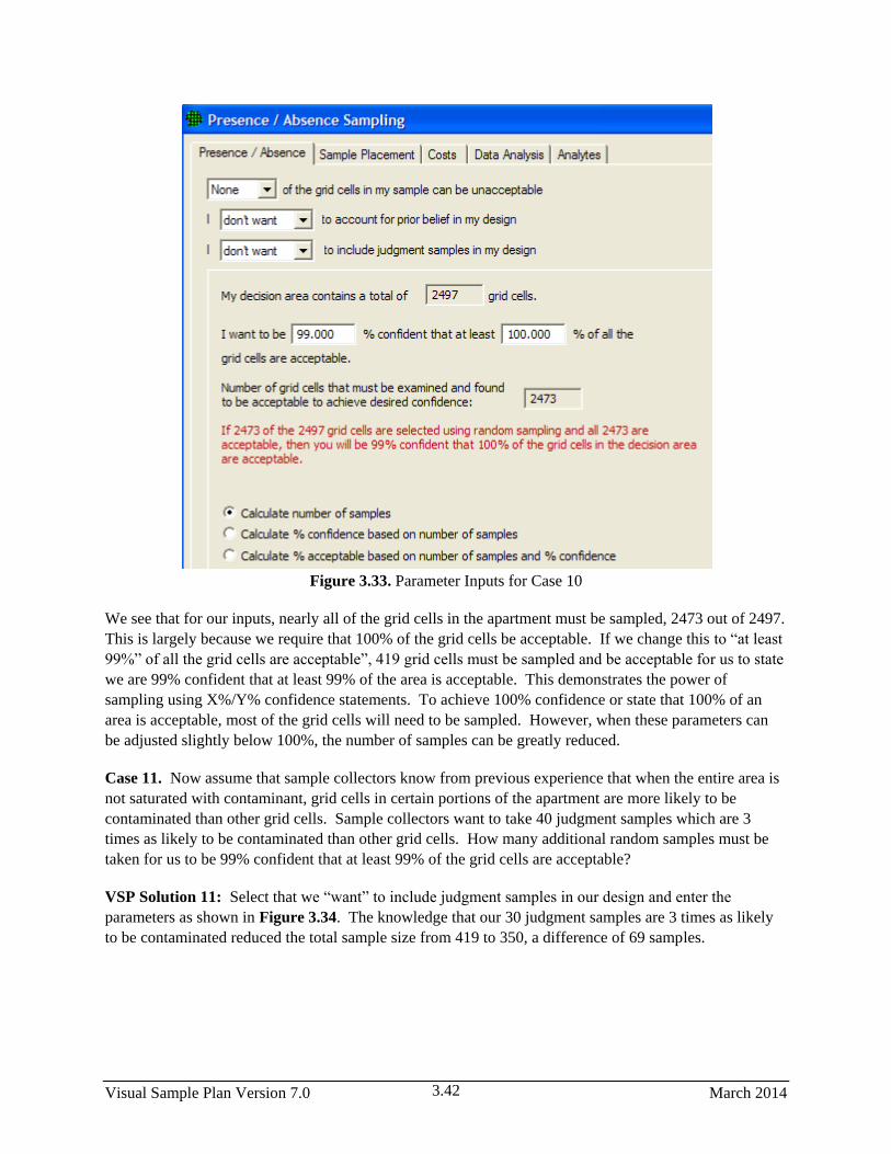
Visual Sample Plan Version 7.0 March 2014 3.42
Figure 3.33. Parameter Inputs for Case 10
We see that for our inputs, nearly all of the grid cells in the apartment must be sampled, 2473 out of 2497.
This is largely because we require that 100% of the grid cells be acceptable. If we change this to “at least
99%” of all the grid cells are acceptable”, 419 grid cells must be sampled and be acceptable for us to state
we are 99% confident that at least 99% of the area is acceptable. This demonstrates the power of
sampling using X%/Y% confidence statements. To achieve 100% confidence or state that 100% of an
area is acceptable, most of the grid cells will need to be sampled. However, when these parameters can
be adjusted slightly below 100%, the number of samples can be greatly reduced.
Case 11. Now assume that sample collectors know from previous experience that when the entire area is
not saturated with contaminant, grid cells in certain portions of the apartment are more likely to be
contaminated than other grid cells. Sample collectors want to take 40 judgment samples which are 3
times as likely to be contaminated than other grid cells. How many additional random samples must be
taken for us to be 99% confident that at least 99% of the grid cells are acceptable?
VSP Solution 11: Select that we “want” to include judgment samples in our design and enter the
parameters as shown in Figure 3.34. The knowledge that our 30 judgment samples are 3 times as likely
to be contaminated reduced the total sample size from 419 to 350, a difference of 69 samples.

March 2014 Visual Sample Plan Version 7.0 3.43
Figure 3.34. Parameter Inputs for Case 11
Case 12: Now assume that sample collectors have previously sampled areas outside and adjacent to the
apartment, and these areas have been cleared. Using their professional experience and judgment, they are
already 90% confident that none of the apartment will be contaminated. They will again take 30
judgment samples which are 3 times as likely to be contaminated as other grid cells. How many samples
must now be taken to be 99% confident that at least 99% of the area is acceptable? What happens if we
reduce the confidence statement to being 95% confident that at least 99% of the area is acceptable? What
about 95% confident that 95% of the area is acceptable.
VSP Solution 12: Select that we “want” to account for prior belief in our design and enter the parameters
as shown in Figure 3.35. We see that the number of samples has been reduced from 350 to 330 using the
prior information that sample collectors were already 90% confident that most of the area would be
acceptable.
Changing the confidence level to 95% further reduces the total number of samples from 330 to 192. The
desired confidence is a key driver in compliance sampling.
Changing the X%/Y% confidence statement to being 95% confident that at least 95% of the area is
acceptable yields a value of “NA” for the number of random samples to be collected. This implies that
the 30 judgment samples being collected satisfies the sampling requirements for the current sampling
design. This is only valid if the statements we make about prior beliefs and judgment sampling locations
are correct. These examples have demonstrated that prior information can drive down sample sizes. Like
all sampling designs, it is important to be sure that assumptions are accurate. Prior beliefs should only be
adjusted if there is evidence and experience that supports it, and not be changed solely for reducing
sample sizes.

Visual Sample Plan Version 7.0 March 2014 3.44
Figure 3.35. Parameter Inputs for Case 12
All of the presence/absence examples presented thus far have been designed so that if any of the samples
are unacceptable, we conclude the area is unacceptable. There is another option where one or more
samples are allowed to be unacceptable. This may be useful in situations where the contaminant of
interest is known to not be dangerous when it is only sparsely located. For this case, we would select
“Some” of the grid cells in my sample can be unacceptable. In addition to the X%/Y% parameters in
other sampling designs, you also enter the Beta level and associated percentage of the site that is
contaminated if we were to assume the alternative hypothesis is true that the area is acceptable. This
design calculates the total number of samples you would need to take to make these confidence
statements if the number of unacceptable samples was the number specified. If the number of grid units
in the sample that are unacceptable exceeds the Acceptance Number, C (which VSP calculates), then the
user concludes the maximum acceptable % of grids contamination has been exceeded and the real
proportion defective is equal to or greater than Pa. The method used for this design is called “Acceptance
Sampling for C > 0”, or just “Acceptance Sampling”. Acceptance Sampling is a test of hypothesis
between two different statements about the number of defective units in the population, Do and Da (Da >
Do). Therefore, Acceptance Sampling for C > 0, requires both an Alpha and a Beta (see Section 3.2).
Refer to the Help for a more complete discussion of the method.
A scenario when Acceptance Sampling for C > 0 may be applicable is that you know some level of
contamination may exist (naturally occurring, or the level of contamination is at the detection level of the
monitoring equipment) to give a lower bound Po, the probability of a defective unit given Do defective

March 2014 Visual Sample Plan Version 7.0 3.45
units are in the population. There is an upper bound Pa (probability when there are Da defective units)
where a health risk may occur and you want to be have a high confidence of detecting contaminating
greater than Pa percent.
3.2.6.2 Using Quantitative Measurements that Follow a Normal Distribution
If the decision unit is large, and the sample support (the amount of material contained in the sample, or
the area swiped for a sample) is small, then point samples are taken under the assumption of an infinite
population of possible sample locations. The assumption of an infinite population eliminates the need for
a finite population correction factor in the sample size calculation. It also eliminates the need to consider
sampling with or without replacement. Random points are generated in the decision unit and samples are
taken at those points.
Methods associated with infinite populations are concerned with percentiles of a population. To test the
null hypothesis that the decision unit is contaminated, we say that if the upper confidence limit on a
percentile of the population is less than the limit, then we can reject the null hypothesis and conclude the
decision unit is uncontaminated. A confidence interval on a percentile of a population is called a
tolerance interval. The tests in this group calculate an Upper tolerance limit (UTL) for the population and
compare it to a limit. The UTL is calculated from sample results. The methods of Upper tolerance limit
are used for infinite populations.
If the decision unit (i.e., a room) is small relative to the sample support, and the sample support is well-
defined (say the sample will consist of a 4 inch square swab), then samples are taken under the
assumption of a finite population of all possible sample locations. We would partition the room into
individual, non-over-lapping “grid” locations, specify the total number of grids in the room, specify the
number of grids to be sampled, then use a random selection of size n (calculated by VSP) grids to be
included in the sample.
Methods associated with finite populations use the concept of “lots”, i.e., a discrete group of units
extracted from a total production run. This has application to a decision unit that can be gridded, with
each grid unit having a discrete identity within the larger population. The methods of Acceptance
sampling (taken from industrial quality control) are used for finite populations. The tests in this group of
methods count the number of grids in the sample that exceed an action level (are defective) and as long as
that number is less than or equal to an “Acceptance Number”, we say the level of contamination is within
the tolerable (i.e., acceptable) limits.

Visual Sample Plan Version 7.0 March 2014 3.46
Figure 3.36. Dialog Input Box for Comparing Percentile of Normal Distribution to Action Level
If the distribution of measurements of contamination at all possible point sample locations in the decision
unit can be considered to be normally distributed (i.e., the standard bell-shaped curve), we can use the
formula that calculates the UTL of a percentile of the normal distribution in the test of the null hypothesis.
This UTL will be compared to the Action Level to determine whether we accept or reject the null
hypothesis. The UTL formula will also be used in the calculation of the sample size, n. Figure 3.36
shows the dialog box for this sampling goal. The design using a parametric upper tolerance limit is select

March 2014 Visual Sample Plan Version 7.0 3.47
from Sampling Goals > Sampling within a Building > Show that at least some high % of the
sampling area is acceptable > Using Quantitative Measurements that Follow a Normal Distribution.
The null hypothesis being tested is that the true Pth percentile of the population exceeds a fixed Action
Level (i.e., the decision unit is contaminated). The user is asked to input the smallest fraction of the
population required to be less than the Action Level in order for the unit to be considered uncontaminated,
input here as 90%. Note: none of the designs discussed below use the Action Level in the sample size
calculation, but Action Level is used in performing the Tests under the Data Analysis tab (see Section 5.6
on Data Analysis). The next set of inputs is the DQO inputs required to calculate sample size. These
inputs are defined in Section 3.2. The Help brings up a screen that describes how these inputs are used to
calculate n. VSP calculates that 47 samples are required to execute the test of the hypothesis with the set
of DQOs listed.
In Figure 3.37 we see the 47 samples located in a room. We drew a room, supplied the inputs for the
Dialog Box, and hit the Apply button. We select View > Room to see the samples located in the room.
Figure 3.37. Samples Placed on Floor and Ceiling Within a Room
3.2.6.3 Using Quantitative Measurements From an Unknown Distribution
Visual Sample Plan Version 7.0 March 2014 3.48
Figure 3.38. Dialog Input Box for Comparing Percentile of
Unknown Distribution to Action Level
If the distribution of measurements is unknown, we must calculate a non-parametric UTL for use in the
test of the hypothesis that the true Pth percentile of the population exceeds a fixed Action Level. This is
accessed from Sampling Goals >
Sampling within a Building > Show
that at least some high % of the
sampling area is acceptable >
Using Quantitative Measurements
From an Unknown Distribution.
The non-parametric UTL happens to
be the largest measurement of the n
samples taken, where n is calculated
using the DQO inputs in Figure 3.38
and the sample size formula
discussed in the VSP Help for this
input screen.
VSP calculates that we need to take
29 samples in order to make a 95%
confidence statement about the 90th
percentile of non-parametric
distribution. The exact wording of
the conclusion that can be drawn is
one of the outputs of VSP. An
example conclusion is shown in red
in Figure 3.38.
3.2.7 Discover Unacceptable Areas With High Confidence
The objective of this design is to discover, with high probability, the presence of unacceptable grid cells if
they exist if a site has been divided into grid cells. This design answers questions like the following,
assuming the probability of a false negative is zero: If 1% of the decision area contained contamination,
how many randomly located samples would I need to take to discover that contamination with 95%
probability?
Discovery sampling requires all surfaces in the decision area be divided into non-overlapping, equal-size
grid cells of specified size that correspond to the sampling methodology. The method may be used
outdoors if the decision area can be divided into grid cells. The size of the grid cell should correspond to
the footprint of the sampling methodology (i.e. the area sampled by the swab, wipe or vacuum, etc.). If
more than one sampling methodology is to be employed in a decision area, the size of the grid cell should
be chosen to match the sampling methodology with the smallest footprint. The location of samples that
will be taken using methodologies with larger footprints should be assigned in a consistent fashion, e.g.
the sample is centered on the smaller grid cell that was assigned by VSP, or the upper-left corner of the
larger sample is aligned with the upper-left corner of the grid cell assigned by VSP, etc. While this
approach to multiple sampling methodologies is conservative, it ensures that the desired confidence level
is preserved.

March 2014 Visual Sample Plan Version 7.0 3.49
Figure 3.39 shows the Dialogue for discover sampling. Here the number of grid cells is shown if using a
map, or it can be entered manually. The other parameters focus on the confidence statement being made.
At the bottom of the dialogue, there are other options besides “Calculate number of samples”. If samples
have already been collected, “Calculate % confidence based on number of samples” can be utilized to
adjust the percent acceptable in the confidence statement and see the corresponding percent confidence.
“Calculate % unacceptable based on number of samples” does the opposite and allows the percent
confidence to be adjusted and shows the percent acceptable in the confidence statement that fits with that
percent confidence.
Figure 3.39. Samples Placed on Floor and Ceiling Within a Room
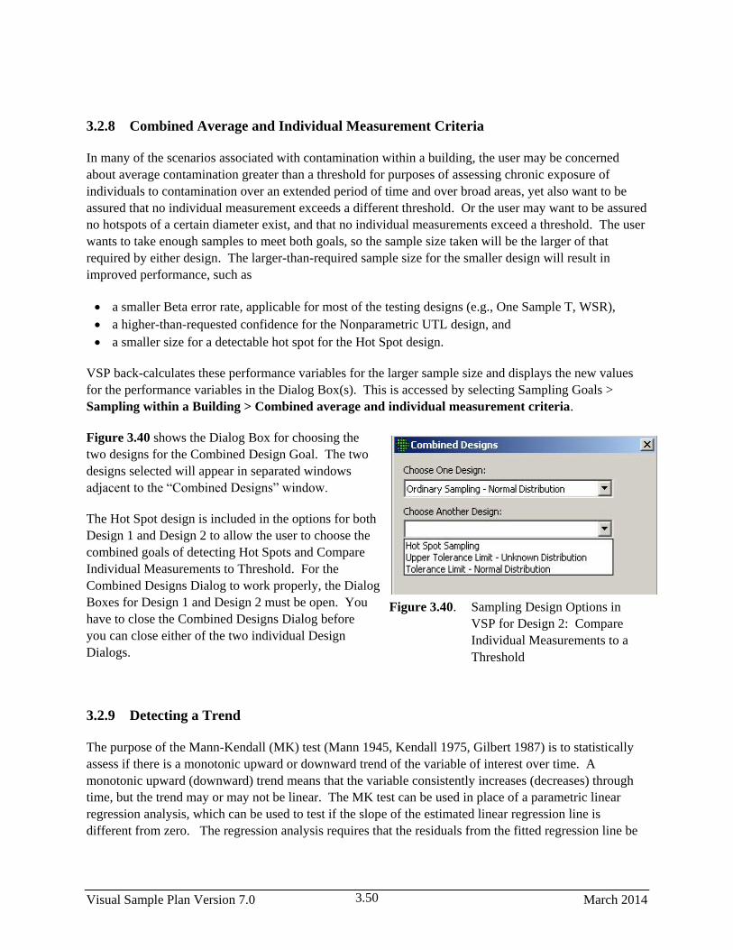
Visual Sample Plan Version 7.0 March 2014 3.50
3.2.8 Combined Average and Individual Measurement Criteria
In many of the scenarios associated with contamination within a building, the user may be concerned
about average contamination greater than a threshold for purposes of assessing chronic exposure of
individuals to contamination over an extended period of time and over broad areas, yet also want to be
assured that no individual measurement exceeds a different threshold. Or the user may want to be assured
no hotspots of a certain diameter exist, and that no individual measurements exceed a threshold. The user
wants to take enough samples to meet both goals, so the sample size taken will be the larger of that
required by either design. The larger-than-required sample size for the smaller design will result in
improved performance, such as
a smaller Beta error rate, applicable for most of the testing designs (e.g., One Sample T, WSR),
a higher-than-requested confidence for the Nonparametric UTL design, and
a smaller size for a detectable hot spot for the Hot Spot design.
VSP back-calculates these performance variables for the larger sample size and displays the new values
for the performance variables in the Dialog Box(s). This is accessed by selecting Sampling Goals >
Sampling within a Building > Combined average and individual measurement criteria.
Figure 3.40 shows the Dialog Box for choosing the
two designs for the Combined Design Goal. The two
designs selected will appear in separated windows
adjacent to the “Combined Designs” window.
The Hot Spot design is included in the options for both
Design 1 and Design 2 to allow the user to choose the
combined goals of detecting Hot Spots and Compare
Individual Measurements to Threshold. For the
Combined Designs Dialog to work properly, the Dialog
Boxes for Design 1 and Design 2 must be open. You
have to close the Combined Designs Dialog before
you can close either of the two individual Design
Dialogs.
3.2.9 Detecting a Trend
The purpose of the Mann-Kendall (MK) test (Mann 1945, Kendall 1975, Gilbert 1987) is to statistically
assess if there is a monotonic upward or downward trend of the variable of interest over time. A
monotonic upward (downward) trend means that the variable consistently increases (decreases) through
time, but the trend may or may not be linear. The MK test can be used in place of a parametric linear
regression analysis, which can be used to test if the slope of the estimated linear regression line is
different from zero. The regression analysis requires that the residuals from the fitted regression line be
Figure 3.40. Sampling Design Options in
VSP for Design 2: Compare
Individual Measurements to a
Threshold

March 2014 Visual Sample Plan Version 7.0 3.51
normally distributed; an assumption not required by the MK test, that is, the MK test is a non-parametric
(distribution-free) test.
Hirsch, Slack and Smith (1982, page 107) indicate that the MK test is best viewed as an exploratory
analysis and is most appropriately used to identify stations where changes are significant or of large
magnitude and to quantify these findings.
To calculate the sample size required for performing a Mann-Kendall test, the dialogue is accessed from
Sampling Goals > Detect a Trend > Residuals not required to be normally distributed > No
Seasonality. A sample dialogue is shown in Figure 3.41.
Figure 3.41. Mann Kendall Design Dialog
We have the options of specifying if we want to detect an upward or downward trend, or both. A linear
model is used if the change over time is expected to be steady. If the change over time is expected to
follow more of a curvilinear pattern, an exponential curve may be a better choice. In Figure 3.41 we
want to detect a downward trend of -1 units per year. VSP calculates that given our input parameters, we
would have to sample for 34 sampling periods (34 months in this case) to collect enough data for
conducting a Mann-Kendall test.
If you suspect there may be seasonal fluctuations in the data, select Sampling Goals > Detect a Trend >
Residuals not required to be normally distributed > Seasonality. In the Seasonal-Kendall test, it is
assumed that sampling is conducted every season. Other than defining the seasons, the dialogue is very
similar to the dialogue for the Mann Kendall test with no seasonality.
Figure 3.42 shows a data analysis window for the Seasonal-Kendall test. The “Testing for Global
Trends” alerts you if trends differ by season or if there are differences between sampling locations. If

Visual Sample Plan Version 7.0 March 2014 3.52
either is the case, then the Seasonal Kendall test results could be misleading. In this case, there appear to
be no global trends, so the downward monotonic trend detected appears to be valid.
Figure 3.42. Data Analysis for Seasonal Kendall Test
Trend Data is often easiest to use by looking at a Time vs. Data plot (Figure 3.43). The raw Values or
model Residuals are plotted against the time variable to help visualize trends over time. In VSP, there are
several options available for customizing the plot:
Show CI: Checking this box allows the user to enter a confidence level. Assuming the model fit is good,
a confidence interval and prediction interval are displayed around the fitted line. The confidence interval
(CI) illustrates the estimated variability around the fitted line. The prediction interval (PI) is a wider
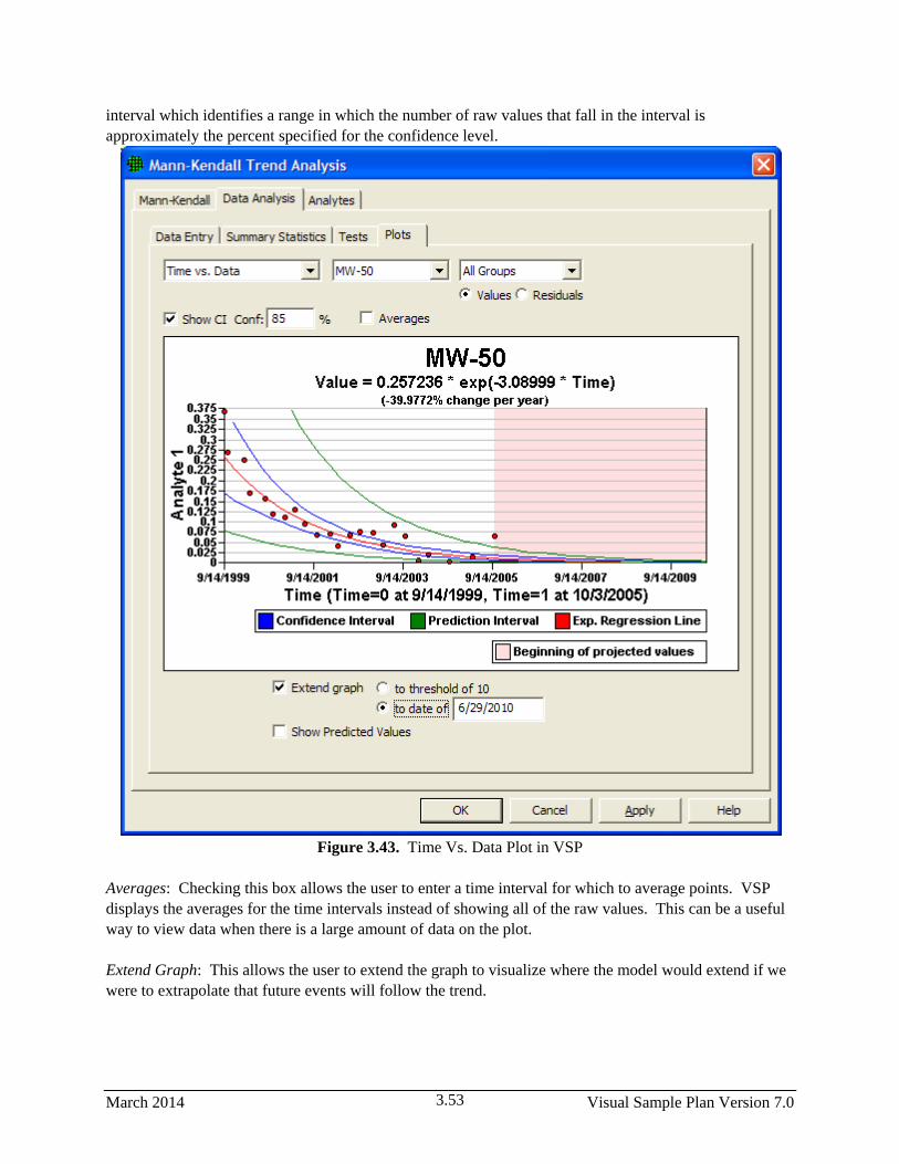
March 2014 Visual Sample Plan Version 7.0 3.53
interval which identifies a range in which the number of raw values that fall in the interval is
approximately the percent specified for the confidence level.
Figure 3.43. Time Vs. Data Plot in VSP
Averages: Checking this box allows the user to enter a time interval for which to average points. VSP
displays the averages for the time intervals instead of showing all of the raw values. This can be a useful
way to view data when there is a large amount of data on the plot.
Extend Graph: This allows the user to extend the graph to visualize where the model would extend if we
were to extrapolate that future events will follow the trend.

Visual Sample Plan Version 7.0 March 2014 3.54
Show Predicted Values: This allows the user to display a column of predicted values generated by a
model outside of VSP. This is done by importing the column and specifying it as a “Predicted” column
while importing.
3.2.10 Identify Sampling Redundancy
The redundancy modules in VSP are used for identifying redundant sample locations (wells), and for
identifying a technically defensible temporal spacing of observations for samples.
3.2.10.1 Analyze Spatial Redundancy
The spatial redundancy module in VSP is based on a geostatistical analysis of spatial sample or well
locations. The algorithm is based on the accumulation of kriging weights to determine a global kriging
weight associated with each sample. The global kriging weight for a given data point is determined by
adding the kriging weights for that data point for all locations in the kriging grid. Global kriging weights
had previously been used by Isaaks and Srivastava (1989) as a method of providing global weights for
individual data points. Cameron and Hunter (2002) used global kriging weights to identify the relative
importance of samples in mapping contaminant plumes, and to identify sample locations or wells that
could be removed from the sampling schedule.
In VSP, sample locations are ranked in terms of their contribution to the plume map through the global
kriging weight, and the lowest ranked data location is removed from the data set. The kriging and ranking
process is then repeated until the maximum number of samples (wells) is removed from the data set. At
each iterative step, the program calculates the root mean square error (RMSE) between the base plume
map and the plume map generated after a given number of sample locations have been removed. The
user then evaluates the number of sample locations that can reasonably be removed from the sampling
schedule by examining the plot of RMSE versus the number of sample locations removed. In addition,
maps showing the plume maps generated using the base case (all sample locations) can be compared with
plume maps generated after eliminating a given number of sample locations.
The analysis is performed using a normal score transform of the data. Transformation of contamination
data is often needed because of their tendency to be highly skewed (Gilbert 1987). The normal score is
widely used in geostatistics because of its ability to transform data with any distribution into a variable
with a perfectly normal (i.e., Gaussian) distribution (Deutsch and Journel 1998). The normal score
transform is also used in the Probability and Uncertainty Mapping module in VSP.
The spatial redundancy module includes several steps:
1. Examine data using data analysis tools and maps
2. Calculate variogram
3. Fit variogram model
4. Determine kriging parameters
5. Complete the spatial analysis
a. Go to Redundancy Analysis tab
b. Choose maximum number of spatial locations (wells) to eliminate from sampling schedule
March 2014 Visual Sample Plan Version 7.0 3.55
c. Hit start to begin process
d. Review results
e. Select number of spatial locations to eliminate from sampling schedule
Steps for Analysis of Redundant Wells using VSP
Step 1 - Examine the data
Before beginning, the data should be examined to ensure that geostatistical analysis is appropriate. At
least 30-50 data points are recommended, and some authors have suggested that the minimum number of
data needed is as much as 100 (e.g., Webster and Oliver 1993), especially for data that exhibit a large
amount of short range variability.
Use the Data Analysis module under the Tools menu in VSP to check for extreme outliers and see
whether the data follow a highly skewed distribution. Kriging also requires the assumption that the data
are spatially continuous, which will be determined during the variogram analysis.
The Exclude column on the Data Entry tab is a binary indicator that indicates whether or not a data point
should be included in the variogram calculations. The user might set the Exclusion indicator to 1 (i.e.,
exclude the point) if a data point is highly redundant. An example might be the large number of wells
present along a remediation barrier. It might be useful to exclude such a large number of highly
redundant points because they can dominate the variogram. The user can calculate the variogram both
with and without points marked for exclusion.
The Reserved column on the Data Entry tab is a binary indicator for whether or not a well should be
included in the well redundancy analysis. In some cases there may be wells that cannot be dropped from
the sampling schedule, for regulatory or other reasons. In that case, they can be included as data points in
kriging, but would not be included in the list of wells that could be removed from the sampling schedule,
even if they appear to be redundant.
Step 2 - Calculate the experimental variogram
What is a variogram? A variogram is a description of the spatial continuity of the data. The experimental
variogram is a discrete function calculated using a measure of variability between pairs of points at
various distances. The exact measure used depends on the variogram type selected (Deutsch & Journel
44-47).
The distances between pairs at which the variogram is calculated are called lags. For instance, lags may
be calculated for samples that are 10 feet apart, then samples that are 20 feet apart, then 30 feet, etc. In
this case the distance between lags is 10 feet. Since points may not be spaced exactly 10 or 20 feet apart,
the lag settings include a lag tolerance value that is typically set to half of the distance between lags. For
the previous example, that would mean that the first lag would include all pairs of points that are between
5 and 15 feet from each other.
Variogram Parameters

Visual Sample Plan Version 7.0 March 2014 3.56
Variogram type:
Select the type of empirical variogram to calculate. The default and recommended first choice is
Semivariogram. Other types can be better for skewed distributions or with the presence of extreme
values. For example, the Semivariogram of logarithms uses logarithmic transform of the data, and
therefore can be useful for log-normally distributed data. The Semivariogram of normal scores uses a
normal score transform of the data (Deutsch and Journel 1998), which can also be helpful for highly
skewed data.
Lag Settings:
Number of lags: Specifies how many lags of the variogram to calculate. This, together with the distance
between lags, determines the maximum distance between pairs of points at which the variogram is
calculated. This maximum distance is called the variogram coverage (number of lags times the distance
between lags), and is displayed on the dialog. The variogram coverage should be less than the site size,
and a good guideline is for the variogram coverage to be closer to ½– ¾ of the site size.
Distance between lags: The intervals to calculate lags. A good distance between lags should be no
smaller than the shortest distance between data points, and should be close to the average spacing of
samples. The ideal lag spacing includes roughly the same number of pairs in each lag, and at least 30
pairs for each lag.
Lag tolerance: How much the distance between pairs can differ from the exact lag distance and still be
included in the lag calculations. The default is ½ of the distance between lags, which ensures that all
possible pairs are included.
Step 3 - Fit a variogram model
Because the kriging algorithm requires a
positive definite model of spatial
variability, the experimental variogram
cannot be used directly. Instead, a model
must be fitted to the data to
approximately describe the spatial
continuity of the data. Certain models
(i.e., mathematical functions) that are
known to be positive definite are used in
the modeling step.
Figure 3.44 shows an experimental
variogram with a variogram model fitted
to it. Each red square is a lag of the
experimental variogram. The x-axis
represents the distance between pairs of
points, and the y-axis represents the
calculated value of the variogram, where Figure 3.44. Variogram Example
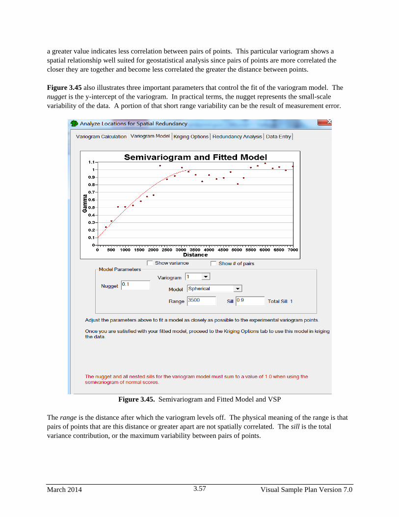
March 2014 Visual Sample Plan Version 7.0 3.57
a greater value indicates less correlation between pairs of points. This particular variogram shows a
spatial relationship well suited for geostatistical analysis since pairs of points are more correlated the
closer they are together and become less correlated the greater the distance between points.
Figure 3.45 also illustrates three important parameters that control the fit of the variogram model. The
nugget is the y-intercept of the variogram. In practical terms, the nugget represents the small-scale
variability of the data. A portion of that short range variability can be the result of measurement error.
Figure 3.45. Semivariogram and Fitted Model and VSP
The range is the distance after which the variogram levels off. The physical meaning of the range is that
pairs of points that are this distance or greater apart are not spatially correlated. The sill is the total
variance contribution, or the maximum variability between pairs of points.
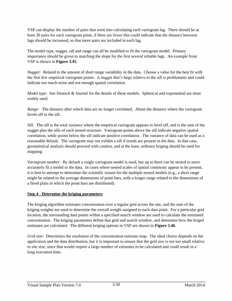
Visual Sample Plan Version 7.0 March 2014 3.58
VSP can display the number of pairs that went into calculating each variogram lag. There should be at
least 30 pairs for each variogram point, if there are fewer this could indicate that the distance between
lags should be increased, so that more pairs are included in each lag.
The model type, nugget, sill and range can all be modified to fit the variogram model. Primary
importance should be given to matching the slope for the first several reliable lags. An example from
VSP is shown in Figure 3.45.
Nugget: Related to the amount of short range variability in the data. Choose a value for the best fit with
the first few empirical variogram points. A nugget that’s large relative to the sill is problematic and could
indicate too much noise and not enough spatial correlation.
Model type: See Deutsch & Journel for the details of these models. Spherical and exponential are most
widely used.
Range: The distance after which data are no longer correlated. About the distance where the variogram
levels off to the sill.
Sill: The sill is the total variance where the empirical variogram appears to level off, and is the sum of the
nugget plus the sills of each nested structure. Variogram points above the sill indicate negative spatial
correlation, while points below the sill indicate positive correlation. The variance of data can be used as a
reasonable default. The variogram may not exhibit a sill if trends are present in the data. In that case,
geostatistical analysis should proceed with caution, and at the least, ordinary kriging should be used for
mapping.
Variogram number: By default a single variogram model is used, but up to three can be nested to more
accurately fit a model to the data. In cases where nested scales of spatial continuity appear to be present,
it is best to attempt to determine the scientific reason for the multiple nested models (e.g., a short range
might be related to the average dimensions of point bars, with a longer range related to the dimensions of
a flood plain in which the point bars are distributed).
Step 4 - Determine the kriging parameters
The kriging algorithm estimates concentration over a regular grid across the site, and the sum of the
kriging weights are used to determine the overall weight assigned to each data point. For a particular grid
location, the surrounding data points within a specified search window are used to calculate the estimated
concentration. The kriging parameters define that grid and search window, and determine how the kriged
estimates are calculated. The different kriging options in VSP are shown in Figure 3.46.
Grid size: Determines the resolution of the concentration estimate map. The ideal choice depends on the
application and the data distribution, but it is important to ensure that the grid size is not too small relative
to site size, since that would require a large number of estimates to be calculated and could result in a
long execution time.

March 2014 Visual Sample Plan Version 7.0 3.59
Kriging type: Ordinary kriging re-estimates the mean within the local search area, this can help account
for trends in the data. Simple kriging uses a constant, site-wide mean, and is the default but the data
distribution and variogram should be examined to see if they support that assumption.
Number of points to use: Minimum and maximum number of data points within the search window to be
used in kriging each estimate. If there isn’t at least the minimum number of points within the search
ellipse, no estimate will be calculated. The maximum number of points to use can also be specified to
limit the computational time required. Larger maximum numbers increase the size of the matrices that
are inverted for the estimation of each grid node, which increases the computational time.
Block kriging: Estimates concentrations for blocks of a specified size instead of a grid of points. Point
kriging is more commonly used in environmental
applications.
Octant search: If octant search is enabled, the search
ellipse is divided into eight equal-angle sectors, and
only the specified maximum number of points from
each octant will be used.
Search ellipsoid: These parameters determine how far
out to search for data to support a particular kriged
estimate.
Max and min horizontal radii: These are the semi-
major and semi-minor axes of the search ellipse,
respectively. They each should be greater than the
range of the variogram model. These values should
only need to differ (i.e. define an ellipse instead of a
circle) if anisotropy is present. Changing the azimuth
angle defining the orientation of the search ellipsoid is
also only necessary for a site with anisotropy.
Step 5 - Complete the well analysis
The analyze tab allows a choice of the maximum
number of wells to remove in the analysis. The
default is all wells available for analysis. If the
maximum to be removed is less than the total number of wells, which will almost always be the case, the
total execution time will be reduced.
After choosing the maximum number of wells to be removed, start the analysis. If the execution appears
to be extremely slow, e.g., a minute passes between each iteration that removes a well, hit the Stop button,
and return to the Kriging tab to increase the size of the X and Y grid cell dimensions.
Once the iterative process is complete, and the wells have been ranked in order of their value, select
“View Maps” (bottom of Figure 3.47) to examine the base map and the map generated with a selected
Figure 3.46. Kriging Options

Visual Sample Plan Version 7.0 March 2014 3.60
number of wells removed. There is no objective measure to determine how many wells can be removed.
However, examination of the RMSE plot provides a measure of the increase in RMSE for removal of
each well, and may suggest thresholds at which large increases in RMSE occur for selection of additional
wells. That, coupled with comparison of maps for different numbers of removed wells, can be used to
select the best number of wells to remove that will decrease sampling costs without adversely impacting
the ability of maps based on the remaining data to adequately represent the plume.
Figure 3.47. Redundant Well Analysis
3.2.10.2 Analyze Temporal Redundancy
The temporal redundancy module in VSP provides methods for examination of the temporal spacing of
observations. The object of the module is to identify a technically defensible temporal spacing. There are
two different sampling goals that are addressed here. One of the main goals is determining if fewer
observations could be used to characterize the contaminant concentrations at a well over time. A second
objective that is sometimes needed is to identify the minimum temporal spacing between observations so
March 2014 Visual Sample Plan Version 7.0 3.61
that they are independent from one another. Methods are included in the module to address both
objectives.
Before performing the analysis, the user may wish to clean the data. The Data Preparation tab in the
Temporal Redundancy module includes tools to select wells for inclusion in the analysis and to remove
large temporal gaps and outliers that may be present in the data.
Single well analysis – Iterative thinning
The iterative thinning approach is based on an algorithm published by Cameron (2004). The goal of the
algorithm is simple, yet elegant: identify the frequency of sampling required to reproduce the temporal
trend of the full data set. The trend may include simple upward or downward trends, but the algorithm
also allows reproduction of more complex patterns, e.g., cyclical patterns related to seasonal variations in
concentration.
The median temporal sample spacing between historical observations is first calculated and used as the
baseline sample spacing. The iterative thinning algorithm uses the Lowess algorithm to fit a smooth trend
and confidence bands (Cleveland 1979) around the full temporal data set. A default bandwidth of 0.5 is
used. See LOWESS Plots for information on the equations used to fit the smooth trend and calculate the
confidence bands around that trend. A percentage of the data points are removed from the data set and
Lowess is used with the same bandwidth to fit a smooth trend to the reduced data set.
The ability of the reduced data set to reproduce the temporal trends in the full data set is evaluated by
calculating the percentage of the data points on the trend for the reduced data set that fall within the 90%
confidence interval established using the full data set. Increasing numbers of data points are removed
from the data set and each of the reduced data sets is evaluated for their ability to reproduce the trend
observed in the full data set. A default level of 75% of the points on the trend for the reduced data falling
within the confidence limits around the original trend is deemed acceptable (Cameron 2004). In order to
guard against artifacts that might arise from the selection of a single set of data points to remove, the
iterative removal process is repeated a large number of times (default number of iterations is 500). The
proportion of data that can be removed while still reproducing the temporal trend of the full data set is
used to estimate an optimal sampling frequency.
Single well analysis – Variogram analysis
The use of variogram analysis for analysis of temporal redundancy has been discussed by several authors,
including Tuckfield (1994), Cameron and Hunter (2002), and Cameron (2004). The first step is to
calculate a temporal variogram for well concentrations, and then fit a variogram model to the
experimental variogram. Given the definition of the range of the variogram model as the lag distance
beyond which data are no longer correlated, the variogram range was proposed by Tuckfield (1994) as an
estimate of a technically defensible sampling frequency.
It should be noted that the goal of that approach was to provide sets of independent samples that could be
used for credible comparisons (e.g., hypothesis testing) of up gradient and down gradient wells (Tuckfield
1994). This would require sampling that would be no more frequent than the temporal variogram range,
so that independent samples would be obtained. This is a valid sampling design goal and for that reason,

Visual Sample Plan Version 7.0 March 2014 3.62
the use of variogram analysis is a valid approach for identifying a defensible temporal sampling
frequency. However, it should be noted that the use of the temporal variogram approach would not define
a sampling frequency that would be best for identifying any temporal trends in the data. If that is the goal
of the analysis, then the iterative thinning approach described above would be more appropriate. Based
on comparisons with data from a large number of wells from different contaminated locations, the
“optimal” sampling frequency identified by the iterative thinning approach is usually much more frequent
than that identified by the variogram range.
The temporal redundancy module includes several steps:
1. Select wells and examine data using data analysis tools
a. May remove outliers based on time gaps or extreme values
2. Choose evaluation method and perform analysis
a. Iterative thinning
b. Variogram analysis
Steps for Analysis of Temporal Redundancy using VSP
Step 1 - Select wells and examine the data
Before beginning, the data should be examined to ensure that the data are appropriate for temporal
redundancy analysis. The Data Preparation tab will exclude all wells with less than 10 observations by
default. Ten wells are usually sufficient for analysis by iterative thinning. However, more observations
would be needed for variogram analysis, usually on the order of 20-30 observations, depending on the
temporal spacing. If variogram analysis will be the primary tool, the user may want to exclude wells with
short time series from the analysis.
The Data Preparation tab allows the user to examine plots of the data to ensure that large time gaps,
outliers, or other problem data are not present. For example, in Figure 3.48 there is a gap in time
between the fifth and sixth observations, identified by the program marking the sixth observation with a
red circle. In addition, it appears that the first five observations were all at a detection limit. If the user
right clicks on any data point, a menu is brought up that allows the user to eliminate a data point, all data
before the data point, or all data after a data point. In this case, it might be appropriate to remove all data
prior to the sixth observation.

March 2014 Visual Sample Plan Version 7.0 3.63
Figure 3.48. Analyze Wells for Temporal Redundancy Dialog
Step 2 - Choose the type of analysis to perform
As discussed above, the main choice to be made is whether to identify a temporal sampling plan that will
allow reproduction of trends seen in the data, or to identify a temporal spacing that should be sufficient to

Visual Sample Plan Version 7.0 March 2014 3.64
ensure that samples are independent of one another. If the first goal is required, perform iterative
thinning, otherwise perform a temporal variogram analysis.
Step 2a - Perform iterative thinning
On the iterative thinning tab, the user first chooses which locations to analyze from the list of available
wells. If the user then hits the Calculate button, the iterative thinning is performed for each of the
selected wells. The results for each well can be viewed by selecting the well from the list in the Analysis
Results.
The display of the results for each well shows the original data, the smoothed curve fit to the data, and a
confidence interval around the smoothed curve (Figure 3.49). The default confidence interval is a 90%
confidence interval.
Beneath the graph for each well will be a statement on the original spacing, the optimal spacing based on
the parameters that were selected, and the reduction in the percentage of samples that would result at the
optimal spacing.
Figure 3.49. View of Smoothed Curve Fit to a Well's Data

March 2014 Visual Sample Plan Version 7.0 3.65
The user can also modify the default parameters used in performing the iterative thinning analysis. By
clicking on the Advanced Options button, the user will be presented with the default settings, and can
modify them, if desired.
Smoothing bandwidth: Related to the width of the smoothing window used in the Lowess smoother.
Default is 0.5, as recommended by Cleveland (1979). Normally set between 0.2 and 0.8. Smaller
bandwidths result in less smoothing of the trend, while wider bandwidths result in greater smoothing.
The choice of bandwidth should also reflect the amount of data available. Small bandwidths should not
be used with sparse time series.
# simulations: The number of Monte Carlo simulations to perform. In each Monte Carlo simulation a
different set of randomly selected samples would be deleted from the base case. The default is 500
simulations. A smaller number would reduce the computational time.
CI confidence: The width of the confidence interval around the smooth trend. Default is set to a 90%
confidence interval. The use of a wider confidence interval (e.g., a 95% CI) will make it more likely that
the smooth trend fit to a reduced dataset will fall within the chosen CI around the base smooth trend, and
thus result in a longer optimal spacing interval. The choice of CI will be documented in the report file.
% of simulated data required within the original trend CI: The default for the percentage of the
simulated trend falling within the original trend CI is 75% (Cameron 2004). The choice of a smaller
percentage will increase the optimal sample spacing. The percentage chosen will be documented in the
report file.
Step 2b - Perform a temporal variogram analysis
The objective of the temporal variogram analysis is to identify the range of the variogram model that best
fits the experimental variogram. The model type, nugget, sill and range can all be modified to fit the
experimental variogram. If a nested model is required (i.e., one showing multiple structures), the range of
interest will be the longest range identified. If an increasing or decreasing trend is present in the
concentration data, then the variogram may increase without breaking over into a sill. In that case, the
variance of the data can be used to identify the sill that must be reached by the model, so that a range can
be identified. The range can then be used as a minimum estimate of the spacing between well samples
that would ensure independence of the samples. A brief description of the parameters of the variogram
model follow:
Nugget: Related to the amount of short range variability in the data. Choose a value for the best fit with
the first few empirical variogram points. A nugget that’s large relative to the sill is problematic and could
indicate too much noise and not enough temporal correlation.
Model type: See Deutsch & Journel or Isaaks and Srivastava for the details of these models. Spherical
and exponential models are most widely used.
Range: The time after which data are no longer correlated: approximately the lag spacing where the
variogram levels off to the sill.
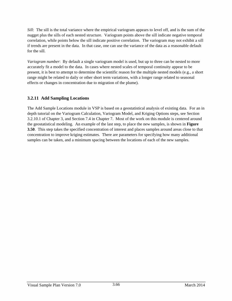
Visual Sample Plan Version 7.0 March 2014 3.66
Sill: The sill is the total variance where the empirical variogram appears to level off, and is the sum of the
nugget plus the sills of each nested structure. Variogram points above the sill indicate negative temporal
correlation, while points below the sill indicate positive correlation. The variogram may not exhibit a sill
if trends are present in the data. In that case, one can use the variance of the data as a reasonable default
for the sill.
Variogram number: By default a single variogram model is used, but up to three can be nested to more
accurately fit a model to the data. In cases where nested scales of temporal continuity appear to be
present, it is best to attempt to determine the scientific reason for the multiple nested models (e.g., a short
range might be related to daily or other short term variations, with a longer range related to seasonal
effects or changes in concentration due to migration of the plume).
3.2.11 Add Sampling Locations
The Add Sample Locations module in VSP is based on a geostatistical analysis of existing data. For an in
depth tutorial on the Variogram Calculation, Variogram Model, and Kriging Options steps, see Section
3.2.10.1 of Chapter 3, and Section 7.4 in Chapter 7. Most of the work on this module is centered around
the geostatistical modeling. An example of the last step, to place the new samples, is shown in Figure
3.50. This step takes the specified concentration of interest and places samples around areas close to that
concentration to improve kriging estimates. There are parameters for specifying how many additional
samples can be taken, and a minimum spacing between the locations of each of the new samples.
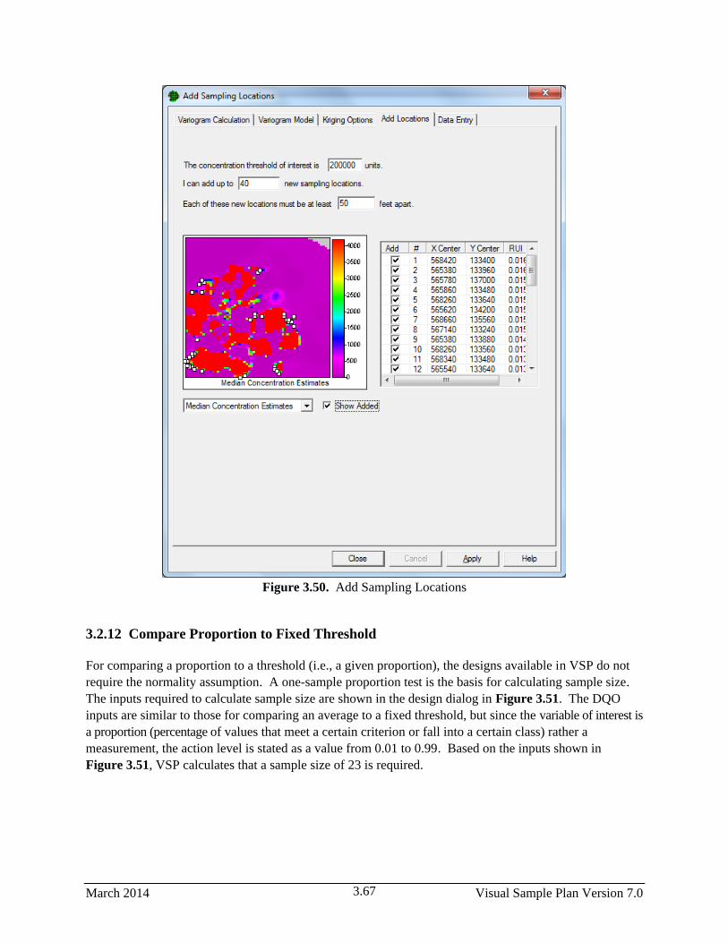
March 2014 Visual Sample Plan Version 7.0 3.67
Figure 3.50. Add Sampling Locations
3.2.12 Compare Proportion to Fixed Threshold
For comparing a proportion to a threshold (i.e., a given proportion), the designs available in VSP do not
require the normality assumption. A one-sample proportion test is the basis for calculating sample size.
The inputs required to calculate sample size are shown in the design dialog in Figure 3.51. The DQO
inputs are similar to those for comparing an average to a fixed threshold, but since the variable of interest is
a proportion (percentage of values that meet a certain criterion or fall into a certain class) rather a
measurement, the action level is stated as a value from 0.01 to 0.99. Based on the inputs shown in
Figure 3.51, VSP calculates that a sample size of 23 is required.
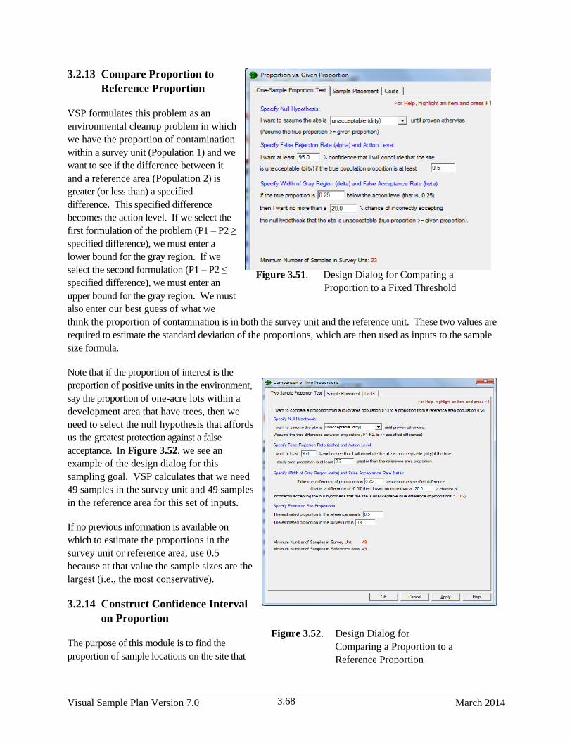
Visual Sample Plan Version 7.0 March 2014 3.68
Figure 3.52. Design Dialog for
Comparing a Proportion to a
Reference Proportion
3.2.13 Compare Proportion to
Reference Proportion
VSP formulates this problem as an
environmental cleanup problem in which
we have the proportion of contamination
within a survey unit (Population 1) and we
want to see if the difference between it
and a reference area (Population 2) is
greater (or less than) a specified
difference. This specified difference
becomes the action level. If we select the
first formulation of the problem (P1 – P2 ≥
specified difference), we must enter a
lower bound for the gray region. If we
select the second formulation (P1 – P2 ≤
specified difference), we must enter an
upper bound for the gray region. We must
also enter our best guess of what we
think the proportion of contamination is in both the survey unit and the reference unit. These two values are
required to estimate the standard deviation of the proportions, which are then used as inputs to the sample
size formula.
Note that if the proportion of interest is the
proportion of positive units in the environment,
say the proportion of one-acre lots within a
development area that have trees, then we
need to select the null hypothesis that affords
us the greatest protection against a false
acceptance. In Figure 3.52, we see an
example of the design dialog for this
sampling goal. VSP calculates that we need
49 samples in the survey unit and 49 samples
in the reference area for this set of inputs.
If no previous information is available on
which to estimate the proportions in the
survey unit or reference area, use 0.5
because at that value the sample sizes are the
largest (i.e., the most conservative).
3.2.14 Construct Confidence Interval
on Proportion
The purpose of this module is to find the
proportion of sample locations on the site that
Figure 3.51. Design Dialog for Comparing a
Proportion to a Fixed Threshold

March 2014 Visual Sample Plan Version 7.0 3.69
have a certain characteristic of concern (such as presence of a contaminant above a specified level or detectable
presence) and compute the upper confidence limit (UCL) on that proportion of samples. You want to be X%
confident that the true proportion of samples on the site that have the characteristic of concern is below the
UCL.
In Figure 3.53, if the user selects “I do not have or do not want to use any prior knowledge about the
expected proportion”, then the expected proportion is 0.5, which will give the most conservative sample
size. Otherwise, to set this value to something other than 0.5, the other option “I am quite sure that the
true proportion of contaminated samples will be less than:” must be selected. In Figure 3.53, it is
expected that the true proportion will be less than 10%, and we want 95% confidence that the true
proportion is less than or equal to 0.15 (0.10 + 0.05), or 15%. The sample size needed is 98.
Figure 3.53. Construct Confidence Interval on a Proportion
In Figure 3.54, the analyte is shown along with several fields. After the user enters the Number of
Samples Obtained and Number of Unacceptable Samples, VSP will calculate the Estimated Proportion
and the Upper Confidence Limit (UCL).
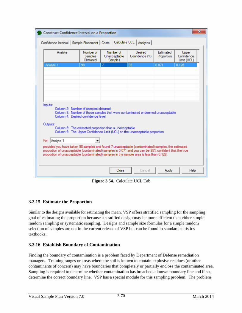
Visual Sample Plan Version 7.0 March 2014 3.70
Figure 3.54. Calculate UCL Tab
3.2.15 Estimate the Proportion
Similar to the designs available for estimating the mean, VSP offers stratified sampling for the sampling
goal of estimating the proportion because a stratified design may be more efficient than either simple
random sampling or systematic sampling. Designs and sample size formulas for a simple random
selection of samples are not in the current release of VSP but can be found in standard statistics
textbooks.
3.2.16 Establish Boundary of Contamination
Finding the boundary of contamination is a problem faced by Department of Defense remediation
managers. Training ranges or areas where the soil is known to contain explosive residues (or other
contaminants of concern) may have boundaries that completely or partially enclose the contaminated area.
Sampling is required to determine whether contamination has breached a known boundary line and if so,
determine the correct boundary line. VSP has a special module for this sampling problem. The problem

March 2014 Visual Sample Plan Version 7.0 3.71
Figure 3.55. Dialog Box for Entering Design Inputs for
Sampling an Enclosing Boundary
and the VSP solution are described in
Visual Sample Plan User’s Guide for
Establishing the Boundary of
Contamination, R.O. Gilbert, et al,
PNWD-3580, 2005, which can be
downloaded from the VSP web site
http://vsp.pnl.gov. In this User’s Guide
we will provide a summary description of
the VSP boundary module.
The VSP sampling design for this
problem involves taking a representative
sample (called a multiple increment or
MI) for each segment along the known,
user-input boundary. If the one or more
samples show contamination, extend or
“bump out” the boundary, and take more
samples. The boundary continues to be
bumped out until all samples taken along
the new boundary line are “clean”.
In Sections 2.3.1.1 and 2.3.1.2 we
described how to define enclosing and
partial boundaries in VSP using Edit >
Sample Areas > Define New Sample
Area, and Edit > Sample Areas >
Define New Open-Type Sample Area,
respectively. VSP determines the
number of segments using the length of the boundary and the specified width of a contaminant plume (hot
spot) that would be of concern if it is present at the boundary or extends beyond the boundary line. VSP
calculates the optimum segment length (OSL) along the current boundary, where all segments have the
same length. One or two MI samples are collected per segment. VSP assumes that each MI sample
collected in a segment consists of 25 small soil samples (increments) that have been collected in sets of 5
small samples clustered around each of 5 equally spaced Primary Sampling Locations along the segment.
The spacing of the five segments depends on the specified width of the hot spot of concern at the
boundary. The OSL is calculated as approximately 5 times the user-specified width of the contamination
plume (hot spot) of concern.
VSP provides two versions of the design: one for enclosing boundaries and one for partial (open-type)
boundaries. Partial boundaries represent a dividing line, with contamination on one side and no
contamination on the other side. VSP provides special tools for creating and manipulating open-type
sample areas.
3.2.16.1 Enclosing Boundary
Menu selection Sampling Goals > Establish Boundary of Contamination > Enclosing Boundary
brings up the dialog box in Figure 3.55 for tab Enclosed Boundary Sampling. The first input required

Visual Sample Plan Version 7.0 March 2014 3.72
Figure 3.56. List of Default Contaminants of
Concern and their Action
Levels
Figure 3.57. An Enclosing Boundary Showing the Segments
and Primary Sampling Locations
is the confidence needed that the mean calculated from limited sample data is indeed less than the action
limit. For this example, that confidence level is 95%. The diameter of the area of contamination (i.e., the
hot spot) that the user wants to be sure is detected at the boundary is input as 45 ft. The next box, labeled
Duplicate Requirements, has to do with how many of the segments need duplicate MI samples to be
collected. VSP requires that: at least 5 segments; or at least 10% of the segments, need duplicates. The
user may select which requirement is used. While 10% is the minimum, the user may input any
percentage for duplicates.
Note: The purpose of duplicate MI samples is to estimate
the relative standard deviation of the data so that an Upper
Confidence Limit (UCL) test can be conducted for each
segment. See VSP Help for more information.
If the boundary of the site is very irregular, e.g., has
various indentations, the VSP user can specify in the
dialogue box that VSP should change the boundary to a
convex hull. This has the effect of smoothing out the
boundary irregularities, but it also enlarges the area
enclosed by the initial boundary. In practice, the VSP user
can try this option and view the resulting initial boundary
to see if the new boundary is acceptable. In Figure 3.55
we leave this box unchecked.
The user now must input the contaminants of
concern and the threshold (action level) at
which we want VSP to trigger extending the
contamination boundary line. The dialog box
for tab Analytes is shown in Figure 3.56. VSP
provides a default list of contaminants of
concern (TNT, RDX, and HMX) and a default
list of upper limit values (Action Limit) for
each (16ppm, 4.4ppm, and 3100ppm). To
remove a contaminant from the list, erase the
name and the limit. To add a contaminant,
enter its name and threshold value in the blank
lint below the last contaminant.
For the Millsite.dxf map file selected, and the
central ellipse in the center of the map selected
as the Sample Area with an enclosing
boundary, we see in Figure 3.57 that after
clicking the Apply button in the previous
screen, VSP divides the boundary into 12
segments. Shown are the 5 equally-spaced
Primary Sampling Locations in each of the
segments. The segments for which the Primary
Sample Locations are in bold type will have

March 2014 Visual Sample Plan Version 7.0 3.73
duplicate samples taken at each location. Different symbols are assigned to each segment to differentiate
the segments visually. For each segment, VSP assumes the user will form the MI sample for that segment
by mixing 5 small soil samples collected from each of the 5 Primary Sampling Locations. Hence, each
MI sample is formed from the 25 small soil samples.
The user now collects the samples, mixes the samples to form a representative MI sample for each
segment, and measures each MI sample. The results are input into VSP using the Sample Information
box that appears when the cursor is placed over one of the Primary Sample Locations, and right-click the
mouse. Use the keyboard to enter the measurement value into the appropriate row in the column labeled
“Value” in the Segment Sample Results sub-box. Use the down arrow button on the keyboard to move
between rows within the sub-box. Figure 3.58 shows the Sample Information Box.
We happened to click on a segment for which two MI samples are required. Thus, we will need to input
two sets of measurements, one for each of the 3 analytes, making 6 input values required. Click the OK
button on the dialog box to close the Sample Information box for that segment. Repeat the above
process for each of the segments to enter all the measurement values. The Segment Sample Results box
has a column headed “UCL”. VSP will fill in this box with the Upper Confidence Limit on the mean
once all the measurement values for the segment are input. The UCL is used to test whether the mean
exceeds the action level for that segment.
Sample results can be entered into VSP using software such as a spreadsheet. Consult VSP’s Help for
instructions on this process.
Figure 3.58. Sample Information Box for Entering Data into VSP, Duplicate Samples Required
VSP now tests whether each boundary segment should be enlarged (bumped out). This is described in an
Appendix to the report PNWD-3580 referenced above. In Figure 3.59 we see an example of two
expanded boundaries. Note the red colored Primary Location Segments indicate that segment did not
pass the UCL test and hence had to be “bumped out”.

Visual Sample Plan Version 7.0 March 2014 3.74
Figure 3.59. Enclosed Boundary with Two Bumped-Out Segments
3.2.16.2 Partial Boundaries
The input screens, the dialog boxes, and the maps for Partial Boundaries problems are similar to those for
the Enclosed Boundaries and will not be shown here. For a discussion of the Partial Boundaries problem
consult the VSP Help function.
3.2.17 UXO Guide
The UXO Guide is a step-by-step guide to choosing the correct design for an unexploded ordnance
(UXO) site. UXO Methods are explained in Chapter 7.
3.2.18 Find UXO Target Areas
This Sampling Goal originated from specific unexploded ordinance (UXO) problems faced by the
Department of Defense. The sampling designs the VSP developers came up with to address these
problems are somewhat specialized. UXO methods are covered in Chapter 7.
3.2.19 Post Remediation Verification Sampling (UXO)
This Sampling Goal also originates from UXO Problems, and is covered in Chapter 7.
3.2.20 Remedial Investigation (UXO)
This Sampling Goal also originates from UXO Problems, and is covered in Chapter 7.

March 2014 Visual Sample Plan Version 7.0 3.75
3.2.21 Sampling Within Buildings
While many of the sampling designs presented in earlier sections could be applied to 3-dimensional
sample areas such as building and rooms (-- as opposed to 2-dimensional sample areas such as land
areas), the sampling designs provided under Sampling within a Building are uniquely suited for problems
where contamination is released into an enclosed structure and contamination can be on walls and
ceilings, windows and doors, as well as on floors, on and under furniture, etc.. Many of the VSP features
added for this module were requested by the Department of Homeland Security (DHS), Combating
Terrorism Technology Support Office. DHS wanted ways to sample walls, floors, ceilings, and other
surfaces to determine if contamination is present, its magnitude and extent throughout the building, and
ways to sample after decontamination to see if the decon was effective.
The sub-goals within this section work through various scenarios when a chemical, biological or
radionuclide release has occurred within a building. Contamination may be isolated, microscopic, and
may selectively adhere to surfaces and crevices. It may be capable of being spread throughout the
building, may pose a health risk at very low levels of contamination, and may be from an unknown source
and released in an unknown location within the building. The unique nature of these contamination
scenarios requires unique sampling methods and unique analysis methods. In the case of a terrorist
bio/chem/rad event, the parameters of interest will most likely be the mean, maximum, or a percentile of
the distribution of all possible measurements. Depending on what the goals are, different sampling
designs will be suggested.
3.2.21.1 Compare Average to a Threshold
A threat analysis team would be interested in average contamination within a building or room if the
primary exposure scenario concerned an accumulated dose, or a long-term exposure of individuals
randomly moving about within the room/building. The sampling goal would be to take samples and
compare the average contamination in a room, or a group of rooms, to a health risk-based threshold.
A number of statistical sampling designs could be applicable depending on the assumptions, constraints,
and sampling technologies. These designs include simple random sampling, grid sampling, sequential
sampling, and collaborative sampling. Similarly, a number of tests could be conducted on the data to
decide if the mean is greater than a threshold. These tests include the one-sample t test and the sign test.
The designs for the sampling goal of comparing an average to a threshold have been discussed earlier in
the manual under the sampling goal of Compare Average to Fixed Threshold (Section 3.2.1).
3.2.21.2 Show That At Least Some High % of the Sampling Area is Acceptable
This option can be applied to buildings and non-buildings, and was explained previously in Section 3.2.6.
3.2.21.3 Locate Hot Spots
The 3-dimension scenario for the hotspot problem is that the user is concerned about hotspots on ceilings
as well as on floors and walls. The extension from the 2-dimensional problem is straightforward. The
floor, ceiling and wall-strip (wall sections laid edge-to-edge) represent three independent surfaces that
might contain a hotspot. Refer to Section 3.2.5 Locating a Hot Spot for a discussion of this sampling
goal.

Visual Sample Plan Version 7.0 March 2014 3.76
3.2.21.4 Combined Average and Individual Measurement Criteria
Refer to Section 3.2.8 for a previous discussion on this methodology.
3.2.22 Radiological Transect Surveying
Radiological transect surveying is supported in VSP. Most of the methods leverage methods originally
implemented in VSP for transect sampling for the detection of unexploded ordnance. For this reason, we
will not go into great depth here as these methods are explained later in Chapter 7.
3.2.22.1 Transect Spacing Needed to Locate a Hot Spot
These methods refer to cases where nearly-continuous measurements are taken along transects (lines or
swaths) and tightly-spaced readings are automatically logged or stored electronically. Because of this
tight spacing, the sampling design for whether or not a transect traverses a hot spot is very robust for the
similar problem of whether or not a radiological survey measurement is taken within a hot spot. The
sampling designs for “Ensure high probability of traversal” and “Manual transect spacing” from the UXO
modules are utilized here. For more information, see VSP’s Help topic under Sampling Goals >
Radiological Transect Surveying > Transect spacing needed to locate a hot spot. Chapter 7, the
UXO methods chapter, also explains how to use these methods, albeit with slightly different terminology.
3.2.22.2 Locate and Mark Hot Spots
This analytical method simply marks points on the map where measurements taken exceeded a specified
threshold.
3.2.22.3 Geostatistical Analysis
Geostatistical analysis of radiological survey data is similar to that of methods for analyzing well
locations on a map. The exception is that radiological surveys can contain many, tightly spaced point
samples. For more information on Geostatistical Analysis, see the Help section in VSP for this module.
Chapter 7 also contains some material on Geostatistical Analysis.
3.2.22.4 Post-Survey Probability of Sampling Within a Hot Spot
This module uses simulation to compute the probability that a survey would have sampled inside a hot
spot of a given size and shape (but unknown location). The user specifies a hot spot of a certain shape
and size on the “Hot Spot” tab as in VSP’s UXO modules. On the “Hot Spot Traversal Simulation” tab,
the user specifies the number of simulations to run. VSP places the center of a hot spot randomly that
number of times within the sample area, and for ellipses generates a random angle of orientation. The hot
spot is traversed if one or more survey measurements lay within the hot spot. The percent of hot spots
detected is reported as a percentage.

March 2014 Visual Sample Plan Version 7.0 3.77
3.2.23 Item Sampling
This module uses the same statistical model as the Compliance Sampling for Presence/Absence module
explained earlier in this chapter. The only difference is that this module uses terminology and
visualizations adapted to sampling of discrete items rather than sampling grid cells on surfaces. An
example of using the item sampling module for sampling 200 drums is shown in Figure 3.60.
Figure 3.60. Example of Item Sampling of Drums
3.2.24 Non-statistical Sampling Approach
VSP allows the user to directly place samples in a Sample Area without going through the Sampling
Goals and the DQO Process. If the user has a pre-determined number of samples, possibly obtained from
a prior DQO study, VSP allows the user to input a sample size and place the samples within the Sample
Area using either a random design or a systematic design. Menu selection Sampling Goals > Non-
Statistical Sampling Approach > Predetermined Number of Samples brings up a simple dialog box
where the user can input any value for Number of Samples, and by hitting the Apply button, the samples
are placed in the Sample Area according to the design specified (random or systematic).
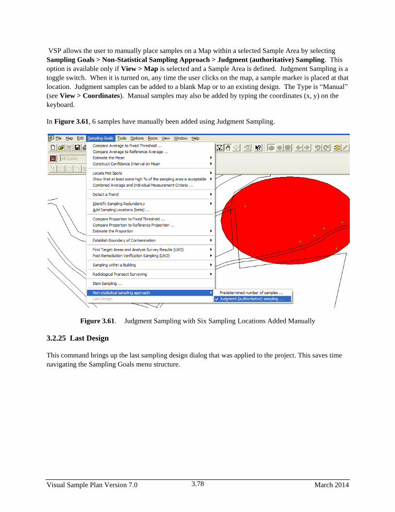
Visual Sample Plan Version 7.0 March 2014 3.78
VSP allows the user to manually place samples on a Map within a selected Sample Area by selecting
Sampling Goals > Non-Statistical Sampling Approach > Judgment (authoritative) Sampling. This
option is available only if View > Map is selected and a Sample Area is defined. Judgment Sampling is a
toggle switch. When it is turned on, any time the user clicks on the map, a sample marker is placed at that
location. Judgment samples can be added to a blank Map or to an existing design. The Type is “Manual”
(see View > Coordinates). Manual samples may also be added by typing the coordinates (x, y) on the
keyboard.
In Figure 3.61, 6 samples have manually been added using Judgment Sampling.
Figure 3.61. Judgment Sampling with Six Sampling Locations Added Manually
3.2.25 Last Design
This command brings up the last sampling design dialog that was applied to the project. This saves time
navigating the Sampling Goals menu structure.

March 2014 Visual Sample Plan Version 7.0 4.1
Figure 4.1. Display of Sampling
Locations on Map
4.0 Assessment of Sampling Plans and View Options
VSP provides multiple displays for allowing you to assess a sampling plan. VSP calls the displays
Views. You can view a representation of the sampling locations on the map entered into VSP, view a graph
of the performance of the design, look at a report that summarizes the key components of the design (such
as number of samples, size of sampling area, cost, probabilities associated with the problem, assumptions,
and technical justification), see a listing of the coordinates of each sampling location. For three
dimensional sampling areas such as buildings and rooms, you can view a 3-D display of the entire
building, and you can also toggle through individual rooms choosing from several ways to display the
rooms. There also is an option which allows for displaying several of these views in different windows
simultaneously. This section describes each of these views and discusses how you can use the views to
assess the VSP sampling plan.
There are two ways to select/change views:
Press one of the display buttons in the middle of the tool bar (MAP VIEW, GRAPH VIEW,
REPORT VIEW, COORDINATE VIEW, 3D VIEW). If you are working with rooms, the
ROOM VIEW may also be used. The QUAD WINDOW button creates 4 separate windows
for displaying multiple views simultaneously.
From the main menu select View > Map (or Graph, Report, Coordinate, Room, 3D)
4.1 Display of Sampling Design on the Map: MAP VIEW button or View >
Map
In Section 2.2, we described how to set up a Map. In
Section 2.3, we described how to set up a Sample Area.
In Section 3.1, we described how to select a Type of
Sampling Plan. In this section, we find out how to
view the results of the sampling design we have just
developed and displayed on the map.
In Figure 4.1, we see the display of a simple triangle we
drew as our map and selected the entire triangle as our
Sample Area. This is available in the file GridSize.vsp,
which is included with the VSP program.
We then selected from the main menu Sampling Goals >
Locate Hot Spots > Assume no false negative errors. We
selected the Probability of Hit to be 90% and selected a
Square grid. We indicated that we wanted to detect a
circular hot spot by selecting a Shape of 1.0 and a Radius
of 4.0 feet. We press Apply, and when we return to the
map (View > Map) we see the 22 samples VSP calculated
as required to meet the sampling goal displayed. Each
time we press Apply, we refresh the map display with a
Visual Sample Plan Version 7.0 March 2014 4.2
new set of random-start sampling locations.
4.2 Display of Cost of Design
In Section 5.4, we describe how to enter costs. For most sampling designs, Total Cost (per unit plus fixed
costs) is tallied and displayed on the same screen where we enter the per-unit costs—under the Costs tab
on the dialog box used for entering design parameters. Cost information is also usually available in the
Report View (View > Report). Reports are discussed in detail in Section 4.4.
4.3 Display of Performance of Design: GRAPH VIEW button or View >
Graph
VSP provides a display of the Performance of the Design for all of the sampling plans that result from
sampling goals where a quantitative decision criterion is supplied. For some sampling goals where the
only criterion the plan must meet is to minimize the variance of the estimate, minimize cost of the
estimate, or to calculate a probability, there is little to graph in terms of the performance of the design.
For such sampling goals, selecting View > Graph brings up a blank graph titled “No Graph”. For some
designs, such as “Detect a Trend”, the Graph view will display a graph of actual data after it is entered
into the Data Analysis page of the design dialog.
For the sampling goals that do specify decision error rates or have confidence bounds on the estimates, VSP
provides a graph of the performance of the sampling design that has just been created. Each sampling
goal, or problem type, has a performance display tailored to it. Each graph tries to show the relationship
between some parameter of the sampling design and how effective that design is at achieving the decision
criteria. Once a Sampling Goal has been selected, the DQO inputs are entered on the dialog box input
screen, and the Apply button is pressed to apply the design to the Sample Area, the display of the
performance can be seen by pressing the GRAPH VIEW button on the tool bar or selecting View >
Graph from VSP’s main menu.
The following sections describe the major displays available for various types of problems. Displays not
described are variants of those presented. Some of the graphs associated with unique sampling designs,
such as Sequential Sampling, have been described in earlier sections, e.g., Graph View of Sequential
Sampling (Figure 3.8), found in Chapter 3. Graphs for UXO-related Sampling Goals are discussed in
Chapter 7.
4.3.1 Performance of Design for Sampling Goal: Compare Average to a Fixed Threshold
The display for the goal of comparing an average to a fixed threshold (i.e., the Action Level) is a graph of
the probability of deciding the true mean of the sample area is greater than or equal to the Action Level on
the vertical (y) axis as opposed to a range of possible true mean values on the horizontal (x) axis. Figure 4.2
is the Decision Performance Goal Diagram (DPGD) described in EPA’s QA/G-4 guidance (EPA 2000a,
pp. 6-7 – 6-11). The document can be downloaded from the EPA at:
http://www.epa.gov/quality/qa_docs.html. Notice how the graph changes as we alternate the null
hypothesis between “Assume Site Dirty” to “Assume Site Clean.”

March 2014 Visual Sample Plan Version 7.0 4.3
The solid vertical red line is positioned at a true mean value of 10, which corresponds to the Action Level.
The area in gray hash marks is the gray region shown here from 8 to 10 and input as a delta (width) of 2. The
two dashed blue lines that extend from the y-axis to the x-axis mark the two types of decision error rates,
alpha, set here at 5%, and beta, set here at 10%. Recall that Alpha is the probability of rejecting the null
hypothesis when it is true (called a false rejection decision error), and beta is the probability of accepting
the null hypothesis when it is false (called a false acceptance decision error). The error rates along with
Figure 4.2. Decision Performance Goal Diagram for Null Hypothesis: True Mean >=Action Level for
Comparing Mean vs. Action Level
the user-supplied standard deviation of 3 and the VSP-calculated sample size n=21 are shown on the second
row of the title. We also see in the title that we are using the sample size formula for the one sample t-test.
The green vertical line marks off one standard deviation (3) from the action level. This mark allows the
user to visually compare the width of the gray region to how variable, on average, we expect individual
observations to be about the mean (definition of standard deviation). The sliding black lines (cross hairs)
that move on the graph when the mouse is moved are provided to facilitate reading the x, y values off the

Visual Sample Plan Version 7.0 March 2014 4.4
graph. This cross-hair feature can be turned off or on by choosing Options > Graph > Display Cross
Hairs.
Most of the parameters displayed on the DPGD can be changed interactively by moving the lines on the
graph, rather than having to change the values in the input dialog box. Table 4.1 describes the interactive
features.
As you change these parameters, you can see the new value of the parameter on the bottom status bar
after “watch here for user input.” You will notice that changing these values on the graph also changes
Table 4.1. Interactive Graph Features
To Change Do the Following
Alpha Drag the horizontal blue dashed line up or down
Beta Drag the horizontal blue dashed line up or down
Delta (and LBGR, or UBGR) Drag the vertical edge of the shaded gray area to the left or right
Standard Deviation Drag the vertical section of the green line left or right
Action Level Drag the vertical red line left or right
Null Hypothesis Click on the y-axis title
these values on the other displays: the sampling design is modified in the report view, new samples are placed
on the map view, and updated sample location information is listed in the coordinate view.
Right-clicking anywhere in the graph brings up a pop-up menu. The options in the menu are described in
Table 4.2. This pop-up menu provides quick access to the menu choices available from the main menu
under Options > Graph. One of the options is to view the complement of the Decision Performance
Goal Diagram, which is referred to as the “Operating Characteristic” Curve. We select this option and the
OC curve is shown in Figure 4.3. Note that the Y-axis is now labeled, “Probability of making the correct
decision”.
Table 4.2. Graph Options Menu Commands
Display Cost Display cost on any graph axis that would otherwise display the number of samples.
Display Cross Hairs Display an interactive cross-hair that allows the user to see the X and Y values for
any point on the graph
Display Current Value Displays a blue dashed cross-hair that corresponds to the current X and Y value
produced by the current sampling design (applies only to certain designs).
Probability of Correct Decision Displays the probability of a correct decision in place of a decision performance
goal diagram
MQO Method Comparison Displays a bar graph that shows the relative costs of MQO sampling design
alternatives.
Barnard’s Log Likelihood Ratio Displays a plot of Barnard’s Log Likelihood Ratio (which is the test statistic used in
Barnard’s sequential t-Test)
Plot Linear Regression Displays the linear regression plot (available for collaborative sampling designs).
Pick UXO Graph Allows user to choose which saved power curve they wish to display in the report
view.

March 2014 Visual Sample Plan Version 7.0 4.5
When the null hypothesis is stated as H0: True Mean ≥ Action Level (Site is Dirty), the gray region is
on the left side of the Action Level. However, when the null hypothesis is stated as H0: True Mean ≤
Action Level (Site is Clean), the gray region is on the right side of the Action Level. In practical terms,
when we assume a site is dirty, the majority of the decision errors will occur for clean sites with true
means just below the Action Level. On the other hand, when we assume a site is clean, the majority of
decision errors will occur for dirty sites with true means just above the Action Level.
The DPGD graph in Figure 4.3 is telling us that for the “Site is Dirty” null hypothesis,
Very clean sites will almost always result in sets of random sampling data that lead to the decision
“Site is Clean.”
Very dirty sites will almost always result in sets of random sampling data that lead to the decision
“Site is Dirty.”
Figure 4.3. Graph of Probability of Making Correct Decision
What we may not know intuitively is how our choice of the null hypothesis affects decisions near the Action
Level. The graph in Figure 4.3 also is telling us
Clean sites with true means just below the Action Level will lead to mostly incorrect decisions.
Dirty sites with true means just above the Action Level will lead to mostly correct decisions.

Visual Sample Plan Version 7.0 March 2014 4.6
Figure 4.4. Decision Performance Goal Diagram for Null Hypothesis: True Mean <= Action Level
for Comparing Mean vs. Action Level
However, when we reverse the null hypothesis and state it as H0: True Mean ≤ Action Level, i.e.,
assume “Site is Clean,” we see in Figure 4.4 that the gray region where the majority of decision errors occur
shifts to the right side of the Action Level. Sites that are dirty now lead to the majority of decision errors.
Also note that alpha is now defined for values less than the action level, while beta is defined for values
above the upper bound of the gray region.
You should carefully study EPA’s QA/G-4 guidance document (EPA 2000a, especially pp. 6-1 to 7-6) to
better understand how to use VSP to balance the choice of null hypothesis, decision error rates, width of the
gray region, total sampling costs, and costs of incorrect decisions.
4.3.2 Performance of Design for Sampling Goal: Construct Confidence Interval on the
Mean
The display for assessing a confidence interval for a mean differs somewhat from that for comparing an
average to a threshold because this is an estimation problem, not a testing problem. As such, there is only
one type of decision error rate, alpha. Shown in Figure 4.5 is the Performance Design for a problem
where the user specified the width of the confidence interval as 1.0, the standard deviation as 3, and a desired
95% one-sided confidence interval on the mean. We are using a one-sided confidence interval (vs. a
two-sided) because we are concerned only about values that exceed the upper bound of the confidence
interval, not values both above the upper bound and below the lower bound. This is consistent with
problems in which the mean to be estimated is average contamination, so we are not concerned about values
below the lower bound of the confidence interval.
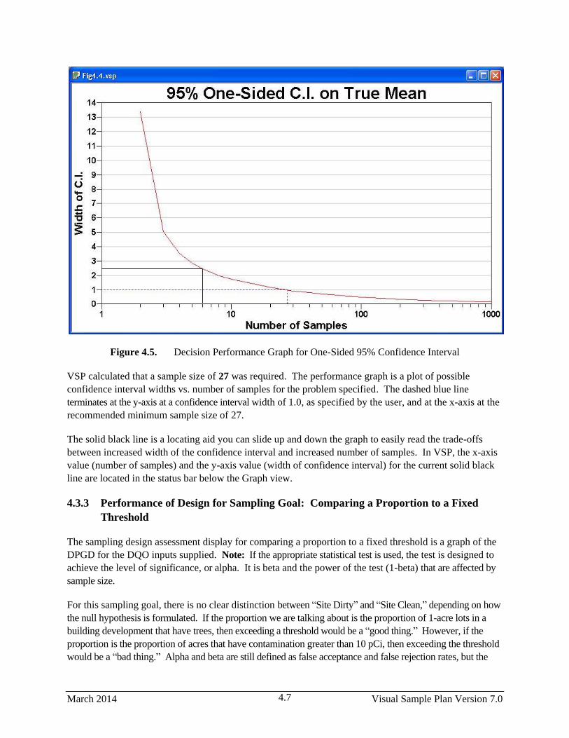
March 2014 Visual Sample Plan Version 7.0 4.7
Figure 4.5. Decision Performance Graph for One-Sided 95% Confidence Interval
VSP calculated that a sample size of 27 was required. The performance graph is a plot of possible
confidence interval widths vs. number of samples for the problem specified. The dashed blue line
terminates at the y-axis at a confidence interval width of 1.0, as specified by the user, and at the x-axis at the
recommended minimum sample size of 27.
The solid black line is a locating aid you can slide up and down the graph to easily read the trade-offs
between increased width of the confidence interval and increased number of samples. In VSP, the x-axis
value (number of samples) and the y-axis value (width of confidence interval) for the current solid black
line are located in the status bar below the Graph view.
4.3.3 Performance of Design for Sampling Goal: Comparing a Proportion to a Fixed
Threshold
The sampling design assessment display for comparing a proportion to a fixed threshold is a graph of the
DPGD for the DQO inputs supplied. Note: If the appropriate statistical test is used, the test is designed to
achieve the level of significance, or alpha. It is beta and the power of the test (1-beta) that are affected by
sample size.
For this sampling goal, there is no clear distinction between “Site Dirty” and “Site Clean,” depending on how
the null hypothesis is formulated. If the proportion we are talking about is the proportion of 1-acre lots in a
building development that have trees, then exceeding a threshold would be a “good thing.” However, if the
proportion is the proportion of acres that have contamination greater than 10 pCi, then exceeding the threshold
would be a “bad thing.” Alpha and beta are still defined as false acceptance and false rejection rates, but the

Visual Sample Plan Version 7.0 March 2014 4.8
user must formulate the hypotheses and select limits on the error rates consistent with the goals of the project
and which type of error is most important to control.
In the example in Figure 4.6, the
null hypothesis was set to True
Proportion ≥ Given
Proportion. As such, beta is
the probability of deciding the
proportion exceeds the threshold
when the true proportion is
equal to or less than the lower
bound of the gray region. For
this problem, we set alpha to
1% and beta to 5%, and the
lower bound of the gray region
to 0.35 (i.e., width of gray
region = 0.15). The proportion
we want to test against (Action
Level) is 0.5. This Action Level
is the most conservative. That
is, the largest number of
samples are needed to
differentiate a proportion from
0.5 (vs. differentiate a
proportion from any other
percentage).
4.3.4 Performance of
Design for Sampling Goal: Compare Average to Reference Average
The sampling design performance display for comparing the true means of two populations when the
assumption of normality can be made is a graph of the probability of deciding if the difference of true
means is greater than or equal to the specified difference (Action Level) vs. various differences of true
means. This graph is similar to the Decision Performance Goal Diagram discussed in Section 4.3.1, but
this time we are dealing with two populations, and the x-axis is a range of possible differences between
the two population means.
The graph shown in Figure 4.7 is for H0: Difference of True Means ≥ Action Level. We revert back to
the notion that this null hypothesis implies a “ Dirty Site” condition. If the action level is a positive
number, we would classify the site as greater than background or “Dirty.” For this problem, the specified
difference of the two means (Action Level) is 5, the width of the gray region is 2, alpha = 5%, beta =
10%, and the estimated common standard deviation = 3.
Figure 4.6. Decision Performance Goal Diagram for
Comparing a Proportion to a Fixed Threshold
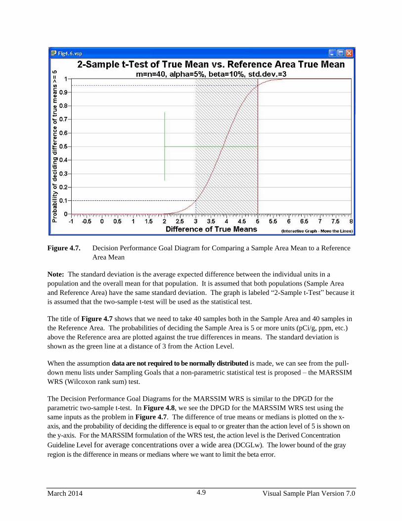
March 2014 Visual Sample Plan Version 7.0 4.9
Figure 4.7. Decision Performance Goal Diagram for Comparing a Sample Area Mean to a Reference
Area Mean
Note: The standard deviation is the average expected difference between the individual units in a
population and the overall mean for that population. It is assumed that both populations (Sample Area
and Reference Area) have the same standard deviation. The graph is labeled “2-Sample t-Test” because it
is assumed that the two-sample t-test will be used as the statistical test.
The title of Figure 4.7 shows that we need to take 40 samples both in the Sample Area and 40 samples in
the Reference Area. The probabilities of deciding the Sample Area is 5 or more units (pCi/g, ppm, etc.)
above the Reference area are plotted against the true differences in means. The standard deviation is
shown as the green line at a distance of 3 from the Action Level.
When the assumption data are not required to be normally distributed is made, we can see from the pull-
down menu lists under Sampling Goals that a non-parametric statistical test is proposed – the MARSSIM
WRS (Wilcoxon rank sum) test.
The Decision Performance Goal Diagrams for the MARSSIM WRS is similar to the DPGD for the
parametric two-sample t-test. In Figure 4.8, we see the DPGD for the MARSSIM WRS test using the
same inputs as the problem in Figure 4.7. The difference of true means or medians is plotted on the x-
axis, and the probability of deciding the difference is equal to or greater than the action level of 5 is shown on
the y-axis. For the MARSSIM formulation of the WRS test, the action level is the Derived Concentration
Guideline Level for average concentrations over a wide area (DCGLw). The lower bound of the gray
region is the difference in means or medians where we want to limit the beta error.
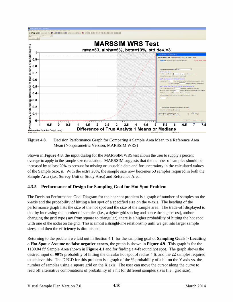
Visual Sample Plan Version 7.0 March 2014 4.10
Figure 4.8. Decision Performance Graph for Comparing a Sample Area Mean to a Reference Area
Mean (Nonparametric Version, MARSSIM WRS)
Shown in Figure 4.8, the input dialog for the MARSSIM WRS test allows the user to supply a percent
overage to apply to the sample size calculation. MARSSIM suggests that the number of samples should be
increased by at least 20% to account for missing or unusable data and for uncertainty in the calculated values
of the Sample Size, n. With the extra 20%, the sample size now becomes 53 samples required in both the
Sample Area (i.e., Survey Unit or Study Area) and Reference Area.
4.3.5 Performance of Design for Sampling Goal for Hot Spot Problem
The Decision Performance Goal Diagram for the hot spot problem is a graph of number of samples on the
x-axis and the probability of hitting a hot spot of a specified size on the y-axis. The heading of the
performance graph lists the size of the hot spot and the size of the sample area. The trade-off displayed is
that by increasing the number of samples (i.e., a tighter grid spacing and hence the higher cost), and/or
changing the grid type (say from square to triangular), there is a higher probability of hitting the hot spot
with one of the nodes on the grid. This is almost a straight-line relationship until we get into larger sample
sizes, and then the efficiency is diminished.
Returning to the problem we laid out in Section 4.1, for the sampling goal of Sampling Goals > Locating
a Hot Spot > Assume no false negative errors, the graph is shown in Figure 4.9. This graph is for the
1130.84 ft2 Sample Area shown in Figure 4.1 and for finding a 4-ft round hot spot. The graph shows the
desired input of 90% probability of hitting the circular hot spot of radius 4 ft. and the 22 samples required
to achieve this. The DPGD for this problem is a graph of the % probability of a hit on the Y axis vs. the
number of samples using a square grid on the X axis. The user can move the cursor along the curve to
read off alternative combinations of probability of a hit for different samples sizes (i.e., grid size).
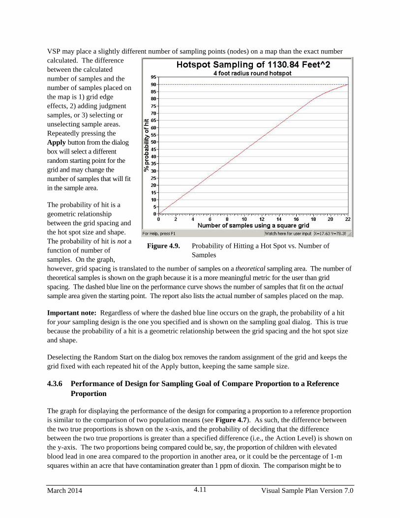
March 2014 Visual Sample Plan Version 7.0 4.11
VSP may place a slightly different number of sampling points (nodes) on a map than the exact number
calculated. The difference
between the calculated
number of samples and the
number of samples placed on
the map is 1) grid edge
effects, 2) adding judgment
samples, or 3) selecting or
unselecting sample areas.
Repeatedly pressing the
Apply button from the dialog
box will select a different
random starting point for the
grid and may change the
number of samples that will fit
in the sample area.
The probability of hit is a
geometric relationship
between the grid spacing and
the hot spot size and shape.
The probability of hit is not a
function of number of
samples. On the graph,
however, grid spacing is translated to the number of samples on a theoretical sampling area. The number of
theoretical samples is shown on the graph because it is a more meaningful metric for the user than grid
spacing. The dashed blue line on the performance curve shows the number of samples that fit on the actual
sample area given the starting point. The report also lists the actual number of samples placed on the map.
Important note: Regardless of where the dashed blue line occurs on the graph, the probability of a hit
for your sampling design is the one you specified and is shown on the sampling goal dialog. This is true
because the probability of a hit is a geometric relationship between the grid spacing and the hot spot size
and shape.
Deselecting the Random Start on the dialog box removes the random assignment of the grid and keeps the
grid fixed with each repeated hit of the Apply button, keeping the same sample size.
4.3.6 Performance of Design for Sampling Goal of Compare Proportion to a Reference
Proportion
The graph for displaying the performance of the design for comparing a proportion to a reference proportion
is similar to the comparison of two population means (see Figure 4.7). As such, the difference between
the two true proportions is shown on the x-axis, and the probability of deciding that the difference
between the two true proportions is greater than a specified difference (i.e., the Action Level) is shown on
the y-axis. The two proportions being compared could be, say, the proportion of children with elevated
blood lead in one area compared to the proportion in another area, or it could be the percentage of 1-m
squares within an acre that have contamination greater than 1 ppm of dioxin. The comparison might be to
Figure 4.9. Probability of Hitting a Hot Spot vs. Number of
Samples
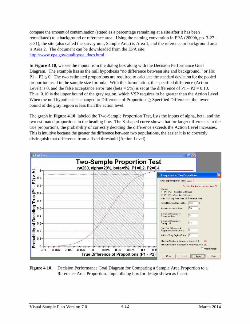
Visual Sample Plan Version 7.0 March 2014 4.12
compare the amount of contamination (stated as a percentage remaining at a site after it has been
remediated) to a background or reference area. Using the naming convention in EPA (2000b, pp. 3-27 –
3-31), the site (also called the survey unit, Sample Area) is Area 1, and the reference or background area
is Area 2. The document can be downloaded from the EPA site:
http://www.epa.gov/quality/qa_docs.html.
In Figure 4.10, we see the inputs from the dialog box along with the Decision Performance Goal
Diagram. The example has as the null hypothesis “no difference between site and background,” or Ho:
P1 – P2 ≤ 0. The two estimated proportions are required to calculate the standard deviation for the pooled
proportion used in the sample size formula. With this formulation, the specified difference (Action
Level) is 0, and the false acceptance error rate (beta = 5%) is set at the difference of P1 – P2 = 0.10.
Thus, 0.10 is the upper bound of the gray region, which VSP requires to be greater than the Action Level.
When the null hypothesis is changed to Difference of Proportions ≥ Specified Difference, the lower
bound of the gray region is less than the action level.
The graph in Figure 4.10, labeled the Two-Sample Proportion Test, lists the inputs of alpha, beta, and the
two estimated proportions in the heading line. The S-shaped curve shows that for larger differences in the
true proportions, the probability of correctly deciding the difference exceeds the Action Level increases.
This is intuitive because the greater the difference between two populations, the easier it is to correctly
distinguish that difference from a fixed threshold (Action Level).
Figure 4.10. Decision Performance Goal Diagram for Comparing a Sample Area Proportion to a
Reference Area Proportion. Input dialog box for design shown as insert.

March 2014 Visual Sample Plan Version 7.0 4.13
4.3.7 Performance of Design for Sampling Goal of Establish Boundary of Contamination
In Figure 4.11 we see the performance of the sampling design defined by the inputs shown in Figure
3.36 applied to the Sample Area of the large “oval” in the Millsite.dxf file (see Map View in Figure
3.38). This problem is for the Enclosing Boundary. In order to have a 95% confidence of finding a hot
spot of diameter of 45 ft, we need 12 segments. This dictates we need 60 Primary Sampling Locations
(12 x 5 = 60). The relationship between diameter of hot spot and number of primary sampling locations
is shown in the dashed blue line positioned on the performance curve shown in Figure 4.11. The dashed
line shows the current number of Primary Sampling Locations for this design (n = 60), which may differ
from the optimum number because of rounding and bump-out effects. We can see from the cross hairs
positioned on the performance curve (right-click on graph, and toggle the Display Cross Hairs to “on”),
that if we expand our Primary Sampling Locations to 100, we could detect a hotspot of diameter 27 ft.
with the sample level of 95% confidence.
The sample type of graph is produced for the Open Boundary Sampling Problem.
Figure 4.11. Curve of Trade-off Between Primary Sampling Locations
and Size of Hot Spot that can be Detected

Visual Sample Plan Version 7.0 March 2014 4.14
4.3.8 Performance of Design for Sampling Goal of Remedial Investigation (UXO)
Similar diagnostics graphs have been developed for the Remedial Investigation (UXO) module. These
can be viewed in VSP. These have similarities to diagnostic graphics described in previous sections.
4.4 Display of the Report
One of the most valuable outputs from VSP is the Report that is generated for each application of a
Sampling Design to a Sample Area. The Report View for a sampling design is available by either
selecting the REPORT VIEW button on the toolbar, or by selecting View > Report from the main
menu. The only Sampling Goals that do not produce Reports are Non-statistical sampling approaches
and Comparisons of two proportions.
The Report provides the VSP user with a complete documentation of the sampling design selected. The
report includes:
statement of sampling objective,
the assumptions of the design,
sample size formula,
inputs provided by the user,
summary of VSP outputs including sample size and costs,
list of samples with their coordinates and labels,
map with sample locations identified,
Performance Goal Diagram,
Peer-reviewed technical references for designs and formulas,
technical discussion of the statistical theory supporting the sampling design and sample size formula.
The reports are suitable for incorporation into a quality assurance project plan or a sampling and analysis
plan. The report for some of the sampling designs include:
recommended data analysis activities for how data should be used in the appropriate statistical test to
make a decision,
insight into options presented in the Input Dialog Box,
sensitivity tables showing how sample number changes as input parameters change, and
extended statistical discussions and support equations.
Some of the output from VSP, for some designs, is viewable only within the report. VSP users can use
the information in the Report as an additional source of Help.
A few selections from the report for the selection Sampling Goals > Compare Average to a fixed
threshold, with can assume the data will be normally distributed and ordinary sampling selected, are
shown in Figure 4.12. Each time VSP calculates a new sample size, changes VSP input, or adds points to
an existing design, the report is updated automatically. The complete report can be copied to the

March 2014 Visual Sample Plan Version 7.0 4.15
clipboard for pasting into a word processing application like Microsoft Word by selecting Edit > Copy
from the main menu when the report view is active. The text and graphics are copied using rich text
format (RTF) to preserve formatting. The user opens Microsoft Word, selects Paste, and the entire report
is copied into a Word document.
The sensitivity table in the Report View allows the user to do “what-if” scenarios with VSP input and
output. For the sampling problem shown in Figure 4.12, the sensitivity table shows how sample size
changes with changes in the standard deviation and the two decision error rates, alpha and beta. Different
sampling goals and sets of assumptions have different variables and parameters in their sensitivity table. The user
can change the variables and range of values shown in the sensitivity table by right-clicking anywhere in the
report.
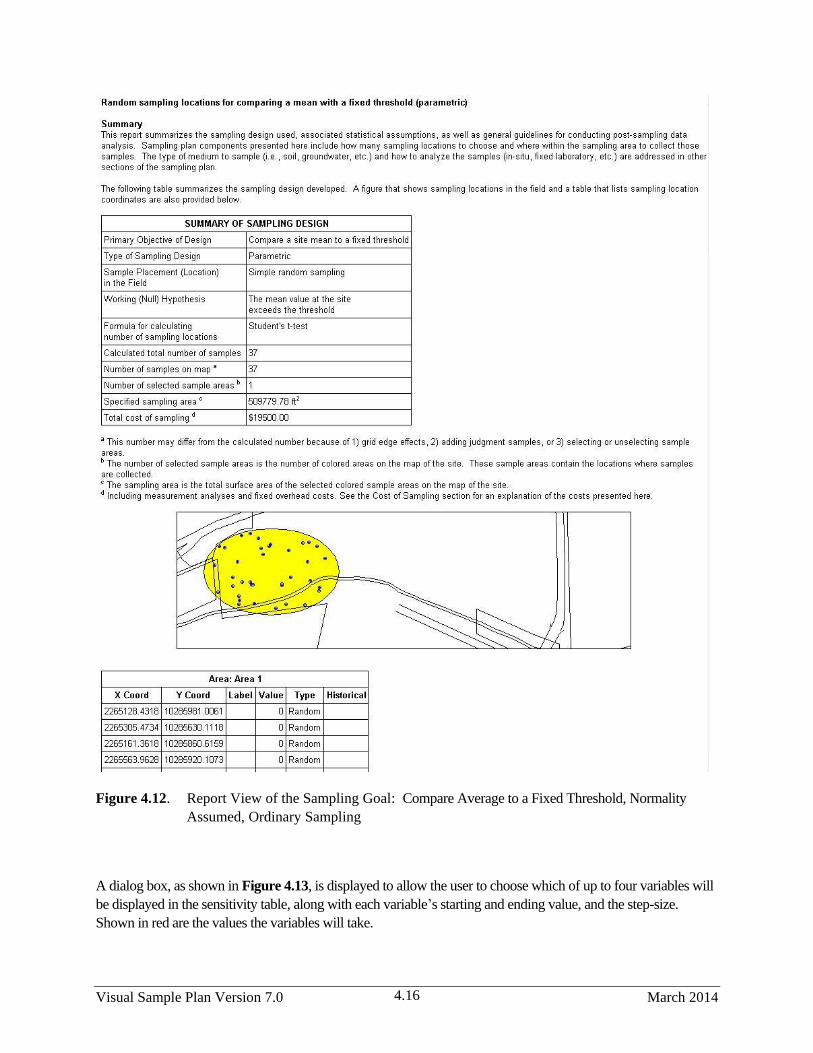
Visual Sample Plan Version 7.0 March 2014 4.16
Figure 4.12. Report View of the Sampling Goal: Compare Average to a Fixed Threshold, Normality
Assumed, Ordinary Sampling
A dialog box, as shown in Figure 4.13, is displayed to allow the user to choose which of up to four variables will
be displayed in the sensitivity table, along with each variable’s starting and ending value, and the step-size.
Shown in red are the values the variables will take.

March 2014 Visual Sample Plan Version 7.0 4.17
Figure 4.14 shows the sensitivity table that will be included in the Report (View > Report). Displayed in
the table can be the number or samples, cost, or both. Certain sampling designs have the option to show
parameters other than cost.
The Report changes based on the Sampling Goal selected. Figures 4.15 and 4.16 show portions of the
Report for the sampling goal of Sampling within a Building. Shown are the two sampling areas: rooms
in yellow are Sampling Room 1; rooms in darker yellow are Sampling Room 2, which is also the Current
Room. In Figure 4.16 we also see the detail on the samples placed within the two rooms, along with
their actual and relative coordinates, type of sample, and whether the sample is placed on the floor,
ceiling, walls, or windows and doors.
Figure 4.13. Dialog Box for Changing Variables Displayed, and Range for Variables Shown, in
Sensitivity Table in Report View. Shown here is input dialog for sampling goal of
compare average to threshold, normality assumed (parametric), ordinary sampling.
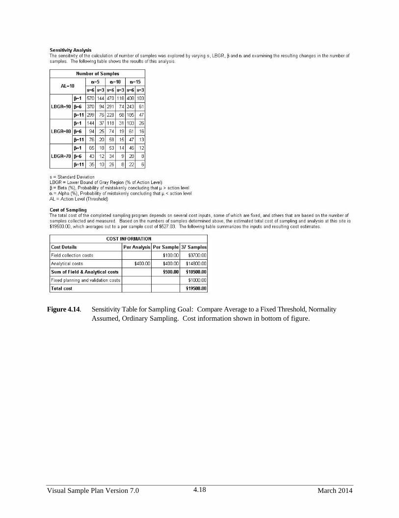
Visual Sample Plan Version 7.0 March 2014 4.18
Figure 4.14. Sensitivity Table for Sampling Goal: Compare Average to a Fixed Threshold, Normality
Assumed, Ordinary Sampling. Cost information shown in bottom of figure.

March 2014 Visual Sample Plan Version 7.0 4.19
Figure 4.15. Report View for Sampling within a Building. Shown are summary information for design
and location of samples areas selected within the floor plan.
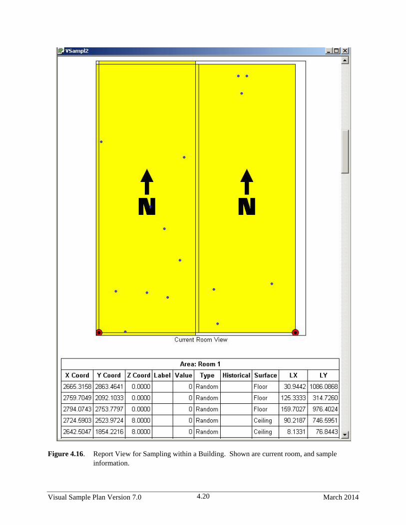
Visual Sample Plan Version 7.0 March 2014 4.20
Figure 4.16. Report View for Sampling within a Building. Shown are current room, and sample
information.

March 2014 Visual Sample Plan Version 7.0 4.21
4.5 Display of Coordinates
The fourth type of display in VSP is the list of coordinates for each sample point on the map. We can see
this display by using the COORDINATE VIEW button on the toolbar, or by selecting Main Menu
option View > Coordinates. The x and y coordinates are displayed for each sample point, and for 3-D sample
areas such as ponds, piles, and rooms, the z-coordinate is also displayed. Also displayed are the sample points
label, a value (if entered by the user), the type (e.g., random, systematic, RSS), and a “true/false” indicator of
whether or not this sample point is a historical sample (previously taken sample). Coordinates are segregated by
Sample Area. These coordinates can be copied and pasted into a spreadsheet or word processing file using Main
Menu option Edit > Copy. Figure 4.17 is an example of the Coordinates view. It should also be noted
that for modules with a Data Entry tab, some of this information can also be viewed there. Additionally,
the analytical modules under Sampling Goals > Find Target Areas and Analyze Survey Results
(UXO) have a Data Entry and Analysis tab used for exporting coordinates to be edited outside of VSP
(see Chapter 7), and the coordinates are not displayed in the COORDINATE VIEW due to these datasets
often being large. If searching for target areas, we don’t display the coordinates. See Chapter 7 for more
information.
Figure 4.17. Coordinates Display of Sampling Locations

Visual Sample Plan Version 7.0 March 2014 4.22
4.6 Multiple Displays
Multiple displays can be brought up on the same screen. Table 4.3 lists the options available under the
main menu item Window.
Table 4.3. Window Menu Commands
New Window Creates a new window that views the same project
Cascade Arranges windows in an overlapped fashion
Tile Arranges windows in non-overlapped tiles.
Arrange Icons Arranges icons of closed windows
Double Window Shows map view and graph view
Triple Window Shows map, graph, and report views
Quad Window Shows map, graph, report, and coordinate views
The user can select the QUAD WINDOW button from the toolbar for a quick way to display the Quad
Window. Figure 4.18 shows the results of the Quad Window option.
Figure 4.18. Quad Display of Map, Graph, Report, and Coordinates on Same Screen

March 2014 Visual Sample Plan Version 7.0 4.23
To summarize, in Figure 4.19 we show the selection of a Sampling Goal and sample type (Simple Random
Sampling), we have entered the DQO inputs into the dialog box, Applied the design to our Sample
Area, and displayed the Map, Graph, Report, and Coordinates simultaneously using the Quad Window
from the Windows menu.
Figure 4.19. Combined Display of VSP Inputs and Outputs
4.7 Room View
Using View > Room displays the current room when working with rooms. This is covered in Chapter 6.
4.8 3D View
The 3D view allows for a three-dimensional view of the map. If the project contains rooms or 3D areas,
they will be shown with proper perspective height. Figure 4.20 shows a building having many rooms
shown in the 3D View.
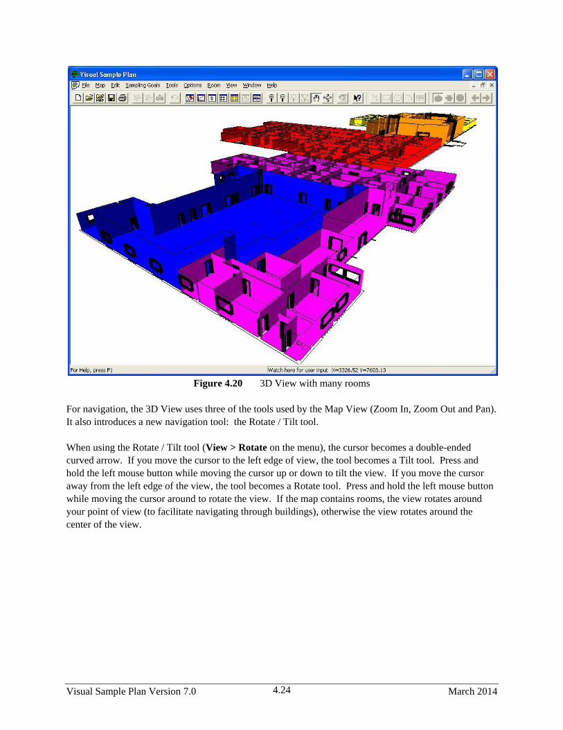
Visual Sample Plan Version 7.0 March 2014 4.24
Figure 4.20 3D View with many rooms
For navigation, the 3D View uses three of the tools used by the Map View (Zoom In, Zoom Out and Pan).
It also introduces a new navigation tool: the Rotate / Tilt tool.
When using the Rotate / Tilt tool (View > Rotate on the menu), the cursor becomes a double-ended
curved arrow. If you move the cursor to the left edge of view, the tool becomes a Tilt tool. Press and
hold the left mouse button while moving the cursor up or down to tilt the view. If you move the cursor
away from the left edge of the view, the tool becomes a Rotate tool. Press and hold the left mouse button
while moving the cursor around to rotate the view. If the map contains rooms, the view rotates around
your point of view (to facilitate navigating through buildings), otherwise the view rotates around the
center of the view.
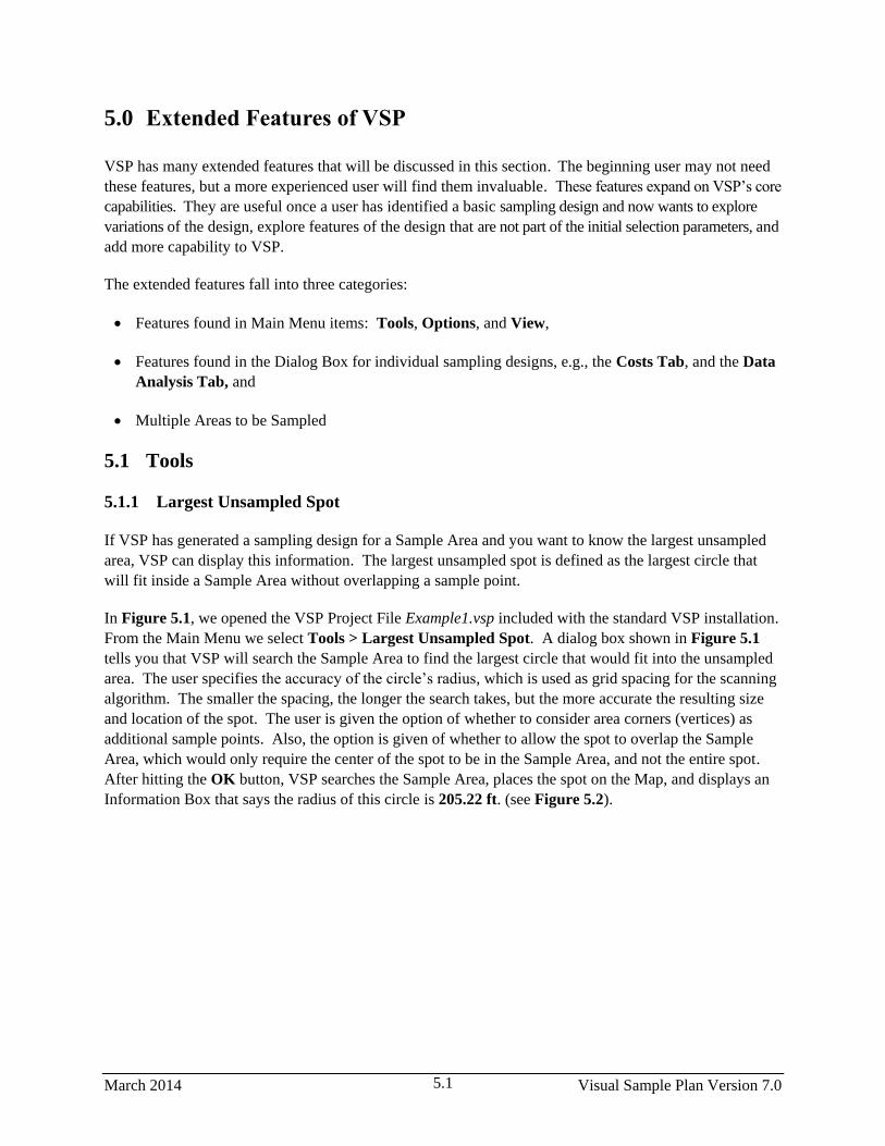
March 2014 Visual Sample Plan Version 7.0 5.1
5.0 Extended Features of VSP
VSP has many extended features that will be discussed in this section. The beginning user may not need
these features, but a more experienced user will find them invaluable. These features expand on VSP’s core
capabilities. They are useful once a user has identified a basic sampling design and now wants to explore
variations of the design, explore features of the design that are not part of the initial selection parameters, and
add more capability to VSP.
The extended features fall into three categories:
Features found in Main Menu items: Tools, Options, and View,
Features found in the Dialog Box for individual sampling designs, e.g., the Costs Tab, and the Data
Analysis Tab, and
Multiple Areas to be Sampled
5.1 Tools
5.1.1 Largest Unsampled Spot
If VSP has generated a sampling design for a Sample Area and you want to know the largest unsampled
area, VSP can display this information. The largest unsampled spot is defined as the largest circle that
will fit inside a Sample Area without overlapping a sample point.
In Figure 5.1, we opened the VSP Project File Example1.vsp included with the standard VSP installation.
From the Main Menu we select Tools > Largest Unsampled Spot. A dialog box shown in Figure 5.1
tells you that VSP will search the Sample Area to find the largest circle that would fit into the unsampled
area. The user specifies the accuracy of the circle’s radius, which is used as grid spacing for the scanning
algorithm. The smaller the spacing, the longer the search takes, but the more accurate the resulting size
and location of the spot. The user is given the option of whether to consider area corners (vertices) as
additional sample points. Also, the option is given of whether to allow the spot to overlap the Sample
Area, which would only require the center of the spot to be in the Sample Area, and not the entire spot.
After hitting the OK button, VSP searches the Sample Area, places the spot on the Map, and displays an
Information Box that says the radius of this circle is 205.22 ft. (see Figure 5.2).
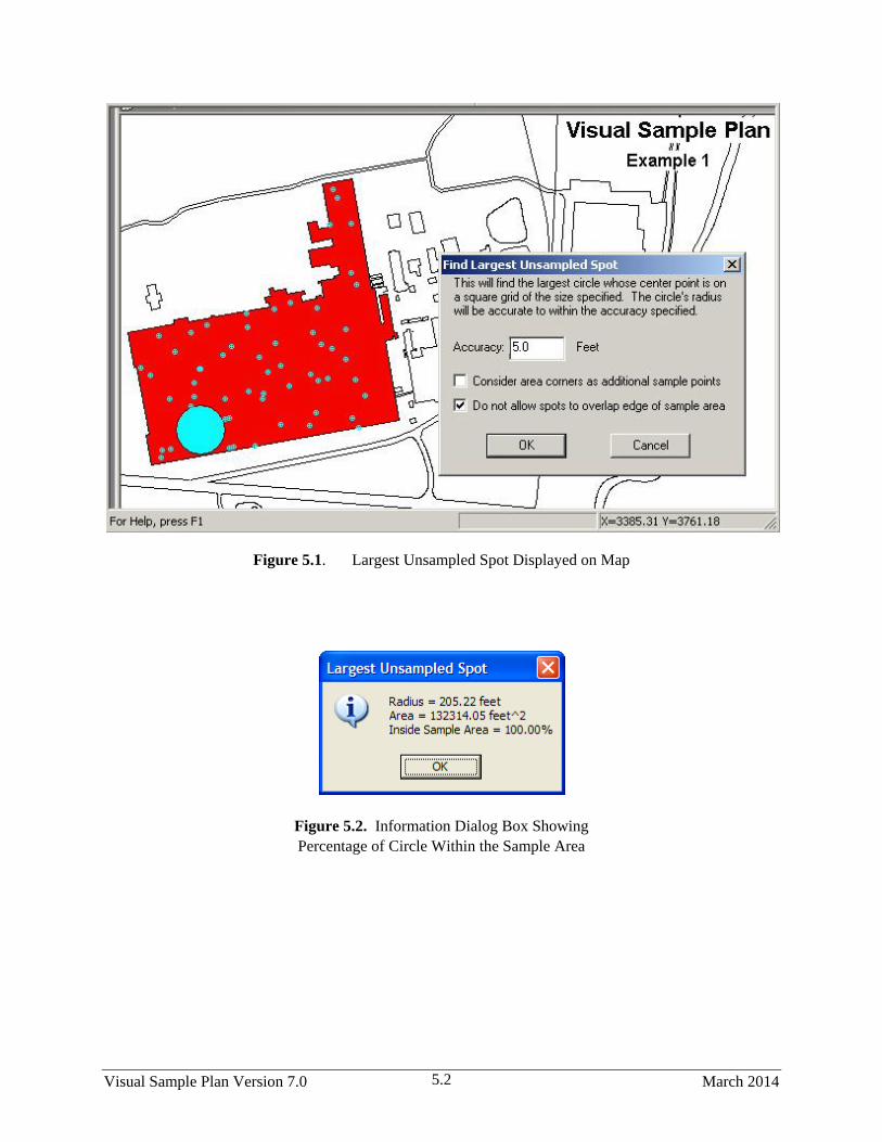
Visual Sample Plan Version 7.0 March 2014 5.2
Figure 5.1. Largest Unsampled Spot Displayed on Map
Figure 5.2. Information Dialog Box Showing
Percentage of Circle Within the Sample Area

March 2014 Visual Sample Plan Version 7.0 5.3
5.1.2 Reset Sampling Design
This command clears the current sampling
design and removes all samples from the map
(including unselected sample areas).
5.1.3 Measure Distance
Use this tool to measure distances on the map.
After selecting this command, the cursor will
become a ruler. Click on the map or enter a
location (x, y) on the keyboard to anchor the
first point. A line will be drawn from the
anchor point to the cursor as you move the
mouse. The status bar will also indicate the
distance from the anchor point to the cursor.
After clicking on a second point or entering a
second point on the keyboard, a dialog will
appear displaying the distance. In Figure 5.3,
we see that the distance from the sampling
point to the building edge is 547.33 ft.
Hold the Shift key down to attach either point
to an existing point on the map.
5.1.4 Make Sample Labels
Individual samples can have labels and values
associated with them. This tool lets the user
design the sample label. Selecting Tools >
Make Sample Labels brings up the Dialog
Box shown in Figure 5.4. VSP assumes the
user will want to assign a unique number to
each sample within a Map, so all labels start
with “VSP-<NNN>”. Other information can
be added to the label, such as the Local X
Coordinate and Local Y Coordinate as shown
in Figure 5.4, by selecting the information
variable names on the list and hitting the Add
button. The information can also be added by
double-clicking on the list item or by typing in
Figure 5.3. Measuring Tool in VSP
Figure 5.4. Dialog Box for Creating Sample Labels
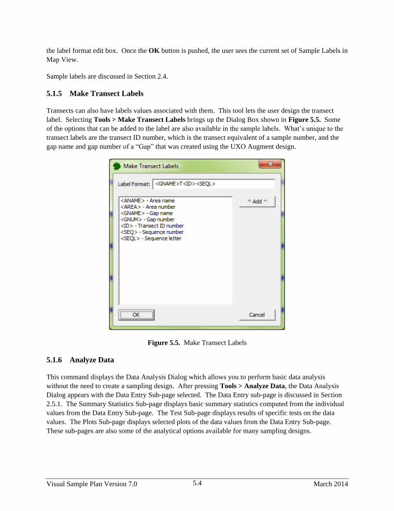
Visual Sample Plan Version 7.0 March 2014 5.4
the label format edit box. Once the OK button is pushed, the user sees the current set of Sample Labels in
Map View.
Sample labels are discussed in Section 2.4.
5.1.5 Make Transect Labels
Transects can also have labels values associated with them. This tool lets the user design the transect
label. Selecting Tools > Make Transect Labels brings up the Dialog Box shown in Figure 5.5. Some
of the options that can be added to the label are also available in the sample labels. What’s unique to the
transect labels are the transect ID number, which is the transect equivalent of a sample number, and the
gap name and gap number of a “Gap” that was created using the UXO Augment design.
Figure 5.5. Make Transect Labels
5.1.6 Analyze Data
This command displays the Data Analysis Dialog which allows you to perform basic data analysis
without the need to create a sampling design. After pressing Tools > Analyze Data, the Data Analysis
Dialog appears with the Data Entry Sub-page selected. The Data Entry sub-page is discussed in Section
2.5.1. The Summary Statistics Sub-page displays basic summary statistics computed from the individual
values from the Data Entry Sub-page. The Test Sub-page displays results of specific tests on the data
values. The Plots Sub-page displays selected plots of the data values from the Data Entry Sub-page.
These sub-pages are also some of the analytical options available for many sampling designs.
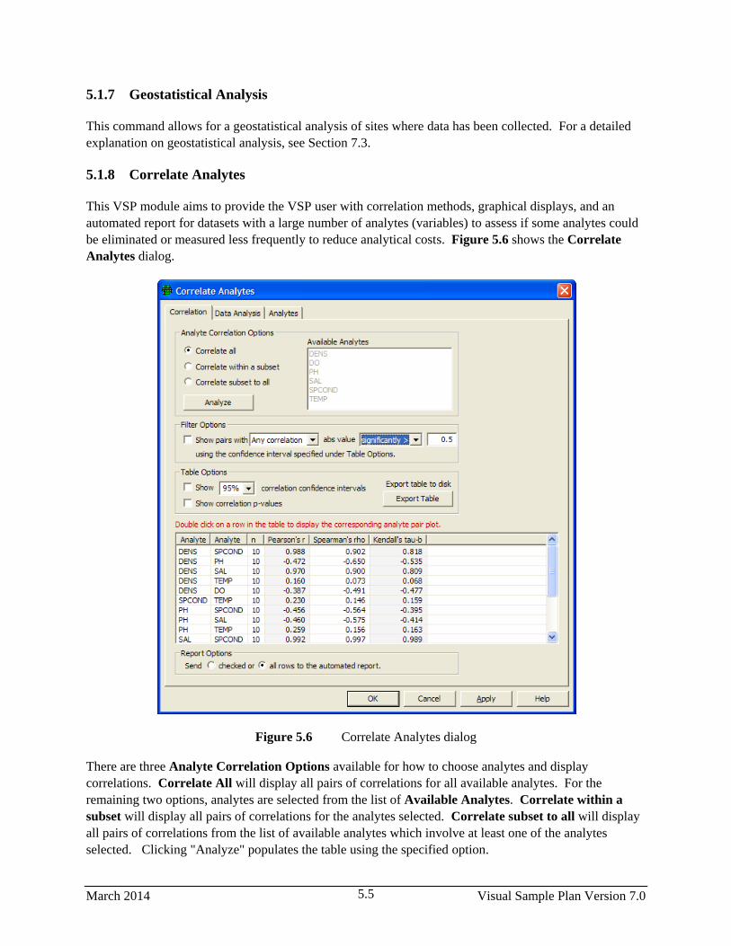
March 2014 Visual Sample Plan Version 7.0 5.5
5.1.7 Geostatistical Analysis
This command allows for a geostatistical analysis of sites where data has been collected. For a detailed
explanation on geostatistical analysis, see Section 7.3.
5.1.8 Correlate Analytes
This VSP module aims to provide the VSP user with correlation methods, graphical displays, and an
automated report for datasets with a large number of analytes (variables) to assess if some analytes could
be eliminated or measured less frequently to reduce analytical costs. Figure 5.6 shows the Correlate
Analytes dialog.
Figure 5.6 Correlate Analytes dialog
There are three Analyte Correlation Options available for how to choose analytes and display
correlations. Correlate All will display all pairs of correlations for all available analytes. For the
remaining two options, analytes are selected from the list of Available Analytes. Correlate within a
subset will display all pairs of correlations for the analytes selected. Correlate subset to all will display
all pairs of correlations from the list of available analytes which involve at least one of the analytes
selected. Clicking "Analyze" populates the table using the specified option.

Visual Sample Plan Version 7.0 March 2014 5.6
Under Filter Options in Figure 5.6, several filters are available for screening out correlations whose
absolute values do not exceed a threshold. Clicking the box next to “Show pairs with” activates this
filter. Then chose the correlations of interest from the drop down menu: Any Correlations, All
Correlations, Pearson’s r, Spearman’s rho, or Kendall’s tau-b. Then select if the absolute value of
this value or values has to be significantly greater than the specified value, or if it simply must be greater
with no condition of significance. Any Correlations implies that if any of Pearson’s r, Spearman’s rho,
or Kendall’s tau-b have absolute values that meet the criteria, the pair of analytes will be displayed. All
Correlations implies that all three correlations must meet the criteria. When Pearson’s r, Spearman’s
rho, or Kendall’s tau-b are selected, only the correlation chosen is tested against the value specified.
The table in Figure 5.6 shows pairs of analytes in the first two columns, and is populated with three
correlations: Pearson’s r, Spearman’s rho, and Kendall’s tau-b. Under Table Options, clicking the
Show correlation confidence intervals box will add confidence intervals to the table for all three
correlations. Clicking the Show correlation p-values box will show the p-value for each correlation for
a test to determine if the correlation is significantly different from zero. Clicking Export table to disk
allows for the table to be exported outside of VSP.
Double-clicking on any row in the table displays a graph of the pair of analytes for that row like the one
shown in Figure 5.7. Checking the Add graph to report box (Figure 5.7), or checking the box in the
left-hand column of the table will insert this plot into the automated report. By default, the entire table is
displayed in the report, but graphs are not automatically displayed if the “checked” button is selected
under Report Options at the bottom of the dialog. To display only checked rows in the table within the
automated report, select the first button under Report Options. Otherwise the report will display all pairs
of analytes shown within the table in the Correlate Analytes dialog.

March 2014 Visual Sample Plan Version 7.0 5.7
Figure 5.7 Analyte Pair Plot
5.1.9 Group Comparison / ANOVA
This tool uses the Analysis of Variance dialog to compare groups of sample results against each other to
find significant differences. To do this, you must first create a Group Type in VSP with two or more
Groups in it. This is done by selecting Edit > Samples > Edit Group List, adding a Group Type, and
then two or more Groups with that Group Type. When you are done creating a Group Type and set of
Groups, select Edit > Samples > Assign To Group to assign samples to a group by clicking around
samples on the map to enclose them in a shape.
Once samples once been assigned to groups, select Tools > Group Comparison / ANOVA and the
dialog in Figure 5.8 will appear. First, select the Analyte you want to use in the comparison. Then select
if you can assume normally distributed data or if you want to make no distributional assumptions. This
determines if a traditional ANOVA will be used or the non-parametric version. Select the Group Type
and then two or more groups that you wish to compare. Finally, select the confidence level you wish to
test with, and a range of dates if you wish to do the comparison on a range of times in the data. At the
bottom of the dialog, the group means, test statistic, and conclusion are shown, and if the initial F-Test
was statistically significant, Group-to-Group Comparisons are shown.
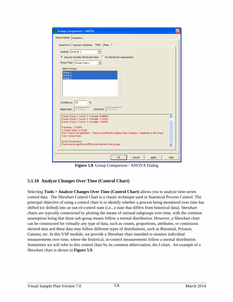
Visual Sample Plan Version 7.0 March 2014 5.8
Figure 5.8 Group Comparison / ANOVA Dialog
5.1.10 Analyze Changes Over Time (Control Chart)
Selecting Tools > Analyze Changes Over Time (Control Chart) allows you to analyze time-series
control data. The Shewhart Control Chart is a classic technique used in Statistical Process Control. The
principal objective of using a control chart is to identify whether a process being monitored over time has
shifted (or drifted) into an out-of-control state (i.e., a state that differs from historical data). Shewhart
charts are typically constructed by plotting the means of rational subgroups over time, with the common
assumption being that these sub-group means follow a normal distribution. However, a Shewhart chart
can be constructed for virtually any type of data, such as counts, proportions, attributes, or continuous
skewed data and these data may follow different types of distributions, such as Binomial, Poisson,
Gamma, etc. In this VSP module, we provide a Shewhart chart intended to monitor individual
measurements over time, where the historical, in-control measurements follow a normal distribution.
Sometimes we will refer to this control chart by its common abbreviation, the I-chart. An example of a
Shewhart chart is shown in Figure 5.9.

March 2014 Visual Sample Plan Version 7.0 5.9
Figure 5.9. Control Chart Example
5.1.11 Interpolated Spatial Maps
Selecting Tools > Interpolated Spatial Maps allows you to interpolate data over an entire site to create a
spatial map using methods other than kriging. Figure 5.10 shows the dialogue for this module. The
available methods are Nearest Neighbor and Inverse Distance Weighting.
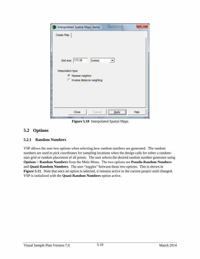
Visual Sample Plan Version 7.0 March 2014 5.10
Figure 5.10 Interpolated Spatial Maps
5.2 Options
5.2.1 Random Numbers
VSP allows the user two options when selecting how random numbers are generated. The random
numbers are used to pick coordinates for sampling locations when the design calls for either a random-
start grid or random placement of all points. The user selects the desired random number generator using
Options > Random Numbers from the Main Menu. The two options are Pseudo-Random Numbers
and Quasi-Random Numbers. The user “toggles” between these two options. This is shown in
Figure 5.11. Note that once an option is selected, it remains active in the current project until changed.
VSP is initialized with the Quasi-Random Numbers option active.
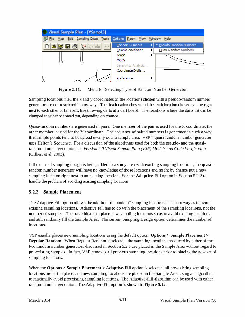
March 2014 Visual Sample Plan Version 7.0 5.11
Figure 5.11. Menu for Selecting Type of Random Number Generator
Sampling locations (i.e., the x and y coordinates of the location) chosen with a pseudo-random number
generator are not restricted in any way. The first location chosen and the tenth location chosen can be right
next to each other or far apart, like throwing darts at a dart board. The locations where the darts hit can be
clumped together or spread out, depending on chance.
Quasi-random numbers are generated in pairs. One member of the pair is used for the X coordinate; the
other member is used for the Y coordinate. The sequence of paired numbers is generated in such a way
that sample points tend to be spread evenly over a sample area. VSP’s quasi-random-number generator
uses Halton’s Sequence. For a discussion of the algorithms used for both the pseudo- and the quasi-
random number generator, see Version 2.0 Visual Sample Plan (VSP) Models and Code Verification
(Gilbert et al. 2002).
If the current sampling design is being added to a study area with existing sampling locations, the quasi--
random number generator will have no knowledge of those locations and might by chance put a new
sampling location right next to an existing location. See the Adaptive-Fill option in Section 5.2.2 to
handle the problem of avoiding existing sampling locations.
5.2.2 Sample Placement
The Adaptive-Fill option allows the addition of “random” sampling locations in such a way as to avoid
existing sampling locations. Adaptive Fill has to do with the placement of the sampling locations, not the
number of samples. The basic idea is to place new sampling locations so as to avoid existing locations
and still randomly fill the Sample Area. The current Sampling Design option determines the number of
locations.
VSP usually places new sampling locations using the default option, Options > Sample Placement >
Regular Random. When Regular Random is selected, the sampling locations produced by either of the
two random number generators discussed in Section 5.2.1 are placed in the Sample Area without regard to
pre-existing samples. In fact, VSP removes all previous sampling locations prior to placing the new set of
sampling locations.
When the Options > Sample Placement > Adaptive-Fill option is selected, all pre-existing sampling
locations are left in place, and new sampling locations are placed in the Sample Area using an algorithm
to maximally avoid preexisting sampling locations. The Adaptive-Fill algorithm can be used with either
random number generator. The Adaptive-Fill option is shown in Figure 5.12.
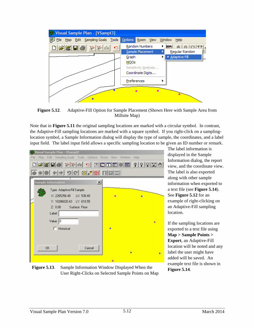
Visual Sample Plan Version 7.0 March 2014 5.12
Figure 5.12. Adaptive-Fill Option for Sample Placement (Shown Here with Sample Area from
Millsite Map)
Note that in Figure 5.11 the original sampling locations are marked with a circular symbol. In contrast,
the Adaptive-Fill sampling locations are marked with a square symbol. If you right-click on a sampling-
location symbol, a Sample Information dialog will display the type of sample, the coordinates, and a label
input field. The label input field allows a specific sampling location to be given an ID number or remark.
The label information is
displayed in the Sample
Information dialog, the report
view, and the coordinate view.
The label is also exported
along with other sample
information when exported to
a text file (see Figure 5.14).
See Figure 5.12 for an
example of right-clicking on
an Adaptive-Fill sampling
location.
If the sampling locations are
exported to a text file using
Map > Sample Points >
Export, an Adaptive-Fill
location will be noted and any
label the user might have
added will be saved. An
example text file is shown in
Figure 5.14. Figure 5.13. Sample Information Window Displayed When the
User Right-Clicks on Selected Sample Points on Map

March 2014 Visual Sample Plan Version 7.0 5.13
Figure 5.14. Sample Exported Text File of Sampling Locations
5.2.3 Graph
Graphs can be displayed with many different options. Figure 5.15 shows the options that can be selected
using Options > Graph. Options are selected by clicking the option on or off. Once selected, that option
will be in place for all Graphs. Note that we saw these same options in Chapter 4, Figure 4.3, by right-
clicking on a Graph. Table 4.2 describes these options in more detail.
Figure 5.15. Graph Options

Visual Sample Plan Version 7.0 March 2014 5.14
5.2.4 Measurement Quality Objectives (MQOs)
The Measurement Quality Objectives (MQO) module in VSP provides a way to extend the sampling design
to consider not only the number and placement of samples in the field but also what happens in the
measurement or analysis process. After all, it is the final result of the “measured sample value” that gets
reported back to the project manager and used in statistical tests to make a decision.
There is a trade-off between taking more samples using a crude (i.e., less precise) measuring device vs.
taking fewer samples using a precise measuring device and/or method. This is because total decision
error is affected by the total standard deviation of the samples. The total standard deviation includes both
sampling variability and analytical measurement variability.
There is also a trade-off between taking more measurements (i.e., replicate measurements) when using
these less precise analytical measuring devices and/or methods vs. taking few measurements and using more
precise analytical measuring devices and/or methods. The MQO module in VSP lets the user play “what-
if” games with various combinations of sampling standard deviation, analytical (i.e., measurement)
standard deviation, number of analyses (i.e., replicates) per sample, and number of samples to take. More
discussion of this topic and the sample size equations behind the VSP calculations can be found in
Version 2.0 Visual Sample Plan (VSP) Models and Code Verification (Gilbert et al. 2002).
Figure 5.16. MQO Input Dialog Box with Default Values Displayed

March 2014 Visual Sample Plan Version 7.0 5.15
The MQO option is selected from the dialog that pops up after a Sampling Design has been selected. The
MQO option can also be toggled using Options > MQOs from the main menu. In Figure 5.16, we see a
dialog box that contains the MQO button (Sampling Goals > Compare Average to Fixed Threshold).
This dialog box allows you to provide additional inputs, such as the analytical standard deviation and
number of analyses per sample.
Note that in situations where analytical methods are highly accurate, values of 0 for the Estimated
Analytical Standard Deviation and 1 for the Analyses per Sample might be used. This means that the
user-selected analytical or measurement method does not add a significant component of variability to the
total standard deviation; i.e., the method provides essentially the same numeric value when repeated
measurements are made on a sample. Using the input parameter values shown in Figure 5.16 and with
these default MQO values, we get n = 21 samples.
Now let’s start changing the MQO input values. First, we change the Estimated Analytical Standard
Deviation to 3. We still take only one analysis per sample. We see VSP now tells us we need to take 40
field samples to obtain the desired error rates we specified. This is shown in Figure 5.17.
Figure 5.17. MQO Input Dialog Box Showing Positive Value for Estimated
Analytical Standard Deviation with 1 Analysis per Sample
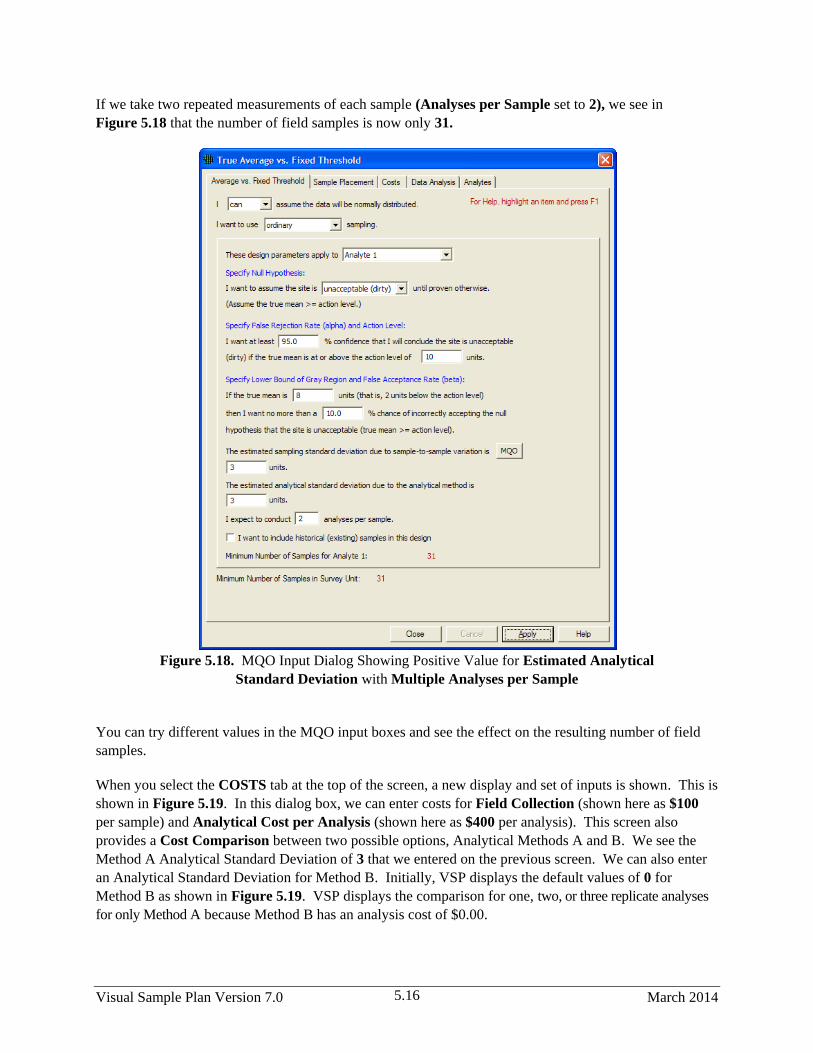
Visual Sample Plan Version 7.0 March 2014 5.16
If we take two repeated measurements of each sample (Analyses per Sample set to 2), we see in
Figure 5.18 that the number of field samples is now only 31.
Figure 5.18. MQO Input Dialog Showing Positive Value for Estimated Analytical
Standard Deviation with Multiple Analyses per Sample
You can try different values in the MQO input boxes and see the effect on the resulting number of field
samples.
When you select the COSTS tab at the top of the screen, a new display and set of inputs is shown. This is
shown in Figure 5.19. In this dialog box, we can enter costs for Field Collection (shown here as $100
per sample) and Analytical Cost per Analysis (shown here as $400 per analysis). This screen also
provides a Cost Comparison between two possible options, Analytical Methods A and B. We see the
Method A Analytical Standard Deviation of 3 that we entered on the previous screen. We can also enter
an Analytical Standard Deviation for Method B. Initially, VSP displays the default values of 0 for
Method B as shown in Figure 5.19. VSP displays the comparison for one, two, or three replicate analyses
for only Method A because Method B has an analysis cost of $0.00.
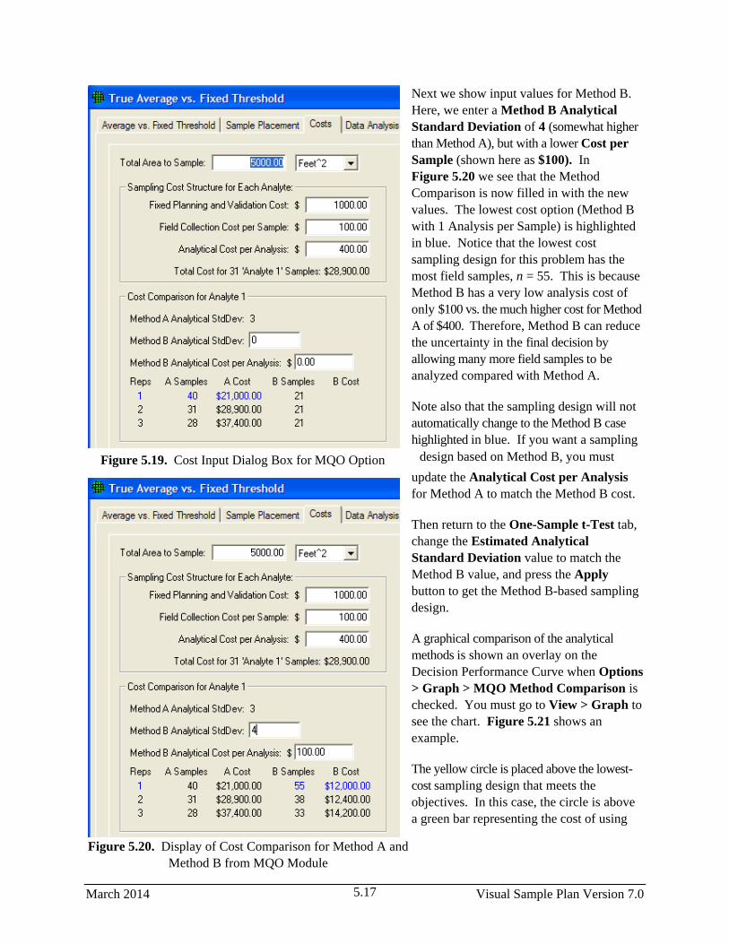
March 2014 Visual Sample Plan Version 7.0 5.17
Next we show input values for Method B.
Here, we enter a Method B Analytical
Standard Deviation of 4 (somewhat higher
than Method A), but with a lower Cost per
Sample (shown here as $100). In
Figure 5.20 we see that the Method
Comparison is now filled in with the new
values. The lowest cost option (Method B
with 1 Analysis per Sample) is highlighted
in blue. Notice that the lowest cost
sampling design for this problem has the
most field samples, n = 55. This is because
Method B has a very low analysis cost of
only $100 vs. the much higher cost for Method
A of $400. Therefore, Method B can reduce
the uncertainty in the final decision by
allowing many more field samples to be
analyzed compared with Method A.
Note also that the sampling design will not
automatically change to the Method B case
highlighted in blue. If you want a sampling
design based on Method B, you must
update the Analytical Cost per Analysis
for Method A to match the Method B cost.
Then return to the One-Sample t-Test tab,
change the Estimated Analytical
Standard Deviation value to match the
Method B value, and press the Apply
button to get the Method B-based sampling
design.
A graphical comparison of the analytical
methods is shown an overlay on the
Decision Performance Curve when Options
> Graph > MQO Method Comparison is
checked. You must go to View > Graph to
see the chart. Figure 5.21 shows an
example.
The yellow circle is placed above the lowest-
cost sampling design that meets the
objectives. In this case, the circle is above
a green bar representing the cost of using
Figure 5.19. Cost Input Dialog Box for MQO Option
Figure 5.20. Display of Cost Comparison for Method A and
Method B from MQO Module
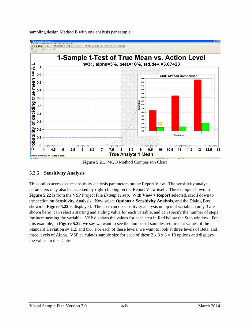
Visual Sample Plan Version 7.0 March 2014 5.18
sampling design Method B with one analysis per sample.
Figure 5.21. MQO Method Comparison Chart
5.2.5 Sensitivity Analysis
This option accesses the sensitivity analysis parameters on the Report View. The sensitivity analysis
parameters may also be accessed by right-clicking on the Report View itself. The example shown in
Figure 5.22 is from the VSP Project File Example1.vsp. With View > Report selected, scroll down to
the section on Sensitivity Analysis. Now select Options > Sensitivity Analysis, and the Dialog Box
shown in Figure 5.22 is displayed. The user can do sensitivity analysis on up to 4 variables (only 3 are
shown here), can select a starting and ending value for each variable, and can specify the number of steps
for incrementing the variable. VSP displays the values for each step in Red below the Step window. For
this example, in Figure 5.22, we say we want to see the number of samples required at values of the
Standard Deviation s= 1.2, and 0.6. For each of these levels, we want to look at three levels of Beta, and
three levels of Alpha. VSP calculates sample size for each of these 2 x 3 x 3 = 18 options and displays
the values in the Table.
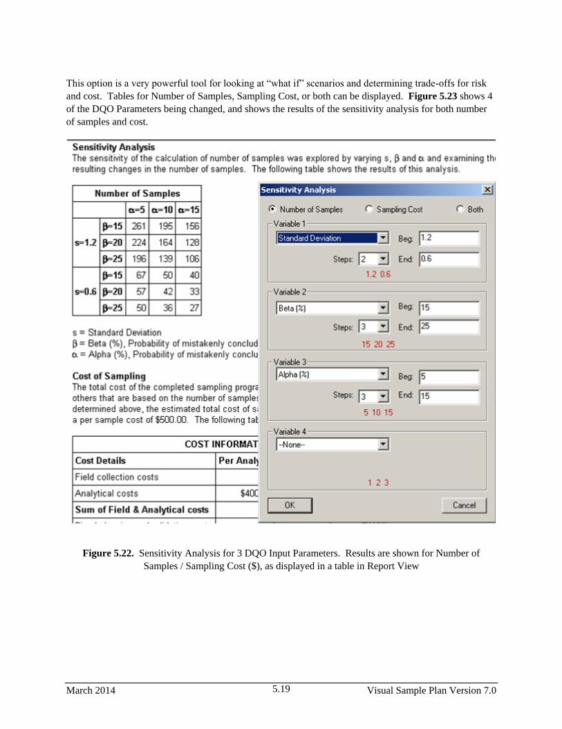
March 2014 Visual Sample Plan Version 7.0 5.19
This option is a very powerful tool for looking at “what if” scenarios and determining trade-offs for risk
and cost. Tables for Number of Samples, Sampling Cost, or both can be displayed. Figure 5.23 shows 4
of the DQO Parameters being changed, and shows the results of the sensitivity analysis for both number
of samples and cost.
Figure 5.22. Sensitivity Analysis for 3 DQO Input Parameters. Results are shown for Number of
Samples / Sampling Cost ($), as displayed in a table in Report View

Visual Sample Plan Version 7.0 March 2014 5.20
Figure 5.23. Sensitivity Analysis for 4 DQO Input Parameters. Results shown for Number of Samples
/ Sampling Cost ($), as displayed in a table in Report View
5.2.6 Coordinate Digits
Selecting this option (Options > Coordinate Digits) brings up a dialog box where the user inputs the
number of significant digits (after the decimal point) for displaying the X, Y, and Z coordinates in View >
Coordinates.
5.2.7 Waypoint Distance
Selecting Options > Waypoint Distance shows the coordinates of transect waypoints in the coordinate
view. Waypoints are intermediate points along the path of long transects. There is a user-defined
maximum spacing between waypoints. This waypoint distance is the maximum distance between
waypoints. Waypoints cannot be imported or pasted into the coordinate view. The import routines expect
the end points of the centerline. See sample data format for more information.
5.2.8 Preferences
Figure 5.24 shows the Preferences available in VSP. Table 5.1 provides a brief description of each
Preference. Consult VSP Help > Help Topics > Menus > Options menu > Preferences for a more
detailed discussion of each menu item.

March 2014 Visual Sample Plan Version 7.0 5.21
Figure 5.24. Preferences Available in VSP
Table 5.1. Preferences Menu Items
Input Delta This preference allows you to input the Delta parameter (width of the gray
region) on all the design dialogs (as opposed to entering the LBGR /
UBGR). This preference setting is persistent (remembered after exiting
and restarting VSP) and affects all project files.
Input LBGR / UBGR This preference allows you to input the Lower Bound of the Gray Region
(LBGR) or the Upper Bound of the Gray Region (UBGR) on all the design
dialogs (as opposed to entering the Delta parameter). This preference
setting is persistent (remembered after exiting and restarting VSP) and
affects all project files.
Version This preference allows you to choose which sub-version of VSP you will
use. The sub-versions of VSP eliminate some features and sampling
designs that do not apply to the general goals of the chosen sub-version.
Initial Information This preference shows you a dialog containing some practical information
to help you use your chosen sub-version of VSP. It also provides some
specialized contact information and help links.
Judgment Sampling Information This option shows an informational dialog each time that judgment
sampling is selected from the menu.
Currency Formatting This preference allows you to change the currency used by VSP and the
way cost values are formatted.
Temporary Directory In order for the geostatistical routines to operate in VSP, temporary files
must be written in the process. By default, VSP uses the temporary
directory that is setup by the Windows system. Using this dialog, you can
change the directory to any location you choose.
Map Units This preference allows you to change what the map coordinate system
units will initially be set to in VSP. As of VSP version 6.1, the default
units of measurement are based on the Windows locale. To override the
locale-specific map units, select the desired Default Map Units on the
drop-down list and press the save button. Checking the Set current project
map to these units will also change the units for the current open project,
otherwise the newly specified default map units will only be used for new

Visual Sample Plan Version 7.0 March 2014 5.22
projects.
5.3 View Menu
The View Menu offers the user options for how VSP displays information. Table 5.2 gives a brief
description of each option. Consult VSP Help > Help Topics > Menus > View menu for a more detail
discussion of each menu item. Many of these items have been discussed previously in this manual and
will be mentioned only briefly here.
Table 5.2. View Menu Items
Main Toolbar Shows or hides the main toolbar
Map Drawing Toolbar Shows or hides the toolbar used for drawing on maps.
Ranked Set Toolbar Shows or hides the toolbar used for ranked set sampling
Room Toolbar Shows or hides the toolbar used for room manipulation
Layer Bar Shows or hides the Layer Control Bar which includes a tree control for accessing
and controlling various map features.
Property Bar Shows or hides the Property Bar for quick access to view and edit the properties
of certain project objects.
Status Bar Shows or hides the status bar.
Labels Shows or hides the sample labels on the map. Any combination of Labels,
Coordinates, Local Coordinates and Values can be displayed.
Largest Unsampled Spots Shows or hides the largest unsampled spots.
All Grid Cells Shows or hides all grid cells used for Grid Cell sampling and Adaptive Cluster
sampling
Grid Lines Shows lines around Grid Cell samples and Adaptive Cluster samples.
Grid Cell Corners Show the corner coordinates of Grid Cell samples and Adaptive Cluster samples
in the coordinate view.
Leading Edge Shows only the leading edge of an open-type sample area
Map Scale Shows or hides the coordinate scale on the map.
Map Legend Shows or hides the map size legend.
Color Legend Shows or hides the color legend.
Transects Transect Corners shows the coordinates at the corners of transects. Waypoints
shows the coordinates of transect waypoints in the coordinate view. Waypoints
are intermediate points along the path of long transects. The Waypoint Distance
is a user-defined maximum spacing between waypoints.
Anomalies Shows or hides the anomaly markers on the map for UXO designs.
Transects Show or hides the transects on the map for UXO designs.
Target Flags Shows or hides the target flags on the map for UXO designs.
Window Densities Shows the window densities on the map. These window densities are generated
by geostatistical mapping of UXO anomaly densities.
Outlier Markers Shows the outlier markers on the map. These window densities are generated by
the UXO Plots page or when comparing two data rasters.
Room North Arrow Shows or hides the north arrow in the room view.
Room Perspective Ceiling Shows or hides the ceiling in the perspective room view.
Map Change current project view to map view.
Graph Change current project view to graph view.
Report Change current project view to report view.
Coordinates Change current project view to coordinate view.
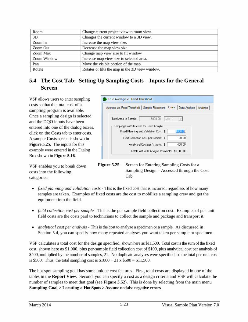
March 2014 Visual Sample Plan Version 7.0 5.23
Figure 5.25. Screen for Entering Sampling Costs for a
Sampling Design – Accessed through the Cost
Tab
Room Change current project view to room view.
3D Changes the current window to a 3D view.
Zoom In Increase the map view size.
Zoom Out Decrease the map view size.
Zoom Max Change map view size to fit window
Zoom Window Increase map view size to selected area.
Pan Move the visible portion of the map.
Rotate Rotates or tilts the map in the 3D view window.
5.4 The Cost Tab: Setting Up Sampling Costs – Inputs for the General
Screen
VSP allows users to enter sampling
costs so that the total cost of a
sampling program is available.
Once a sampling design is selected
and the DQO inputs have been
entered into one of the dialog boxes,
click on the Costs tab to enter costs.
A sample Costs screen is shown in
Figure 5.25. The inputs for this
example were entered in the Dialog
Box shown in Figure 5.16.
VSP enables you to break down
costs into the following
categories:
fixed planning and validation costs - This is the fixed cost that is incurred, regardless of how many
samples are taken. Examples of fixed costs are the cost to mobilize a sampling crew and get the
equipment into the field.
field collection cost per sample - This is the per-sample field collection cost. Examples of per-unit
field costs are the costs paid to technicians to collect the sample and package and transport it.
analytical cost per analysis - This is the cost to analyze a specimen or a sample. As discussed in
Section 5.4, you can specify how many repeated analyses you want taken per sample or specimen.
VSP calculates a total cost for the design specified, shown here as $11,500. Total cost is the sum of the fixed
cost, shown here as $1,000, plus per-sample field collection cost of $100, plus analytical cost per analysis of
$400, multiplied by the number of samples, 21. No duplicate analyses were specified, so the total per-unit cost
is $500. Thus, the total sampling cost is $1000 + 21 x $500 = $11,500.
The hot spot sampling goal has some unique cost features. First, total costs are displayed in one of the
tables in the Report View. Second, you can specify a cost as a design criteria and VSP will calculate the
number of samples to meet that goal (see Figure 3.52). This is done by selecting from the main menu
Sampling Goal > Locating a Hot Spots > Assume no false negative errors.

Visual Sample Plan Version 7.0 March 2014 5.24
Figure 5.26. Proportional Allocation of Samples to
Multiple Sample Areas
5.5 Multiple Areas to be Sampled
VSP allows the user to select multiple areas as sampling areas. All the examples shown so far involved a
single Sample Area. When multiple
areas are selected, VSP allocates the
samples to the areas in proportion to
the area of the respective individual
sample areas. For example, if one area
is twice as large as the other sample
area, it will receive twice as many
sample points, as seen in Figure 5.26.
In Figure 5.26, we show two sample
areas -- a rectangle and a circle. We
next assume that a sampling-design
algorithm not currently in VSP called
for n = 25 samples. Using option
Sampling Goals > Non-statistical
sampling approach > Predetermined
number of samples, VSP allocated 7 of
the 25 requested samples to the
rectangle and 18 to the circle. This is
because the circle covers an area
approximately three times larger than
the rectangle.
Note that when multiple sample areas
are drawn on a Map, you can select or
deselect sample areas using Main Menu option Edit > Sample Areas > Select/Deselect Sample Areas.
Alternatively, you can select or deselect a sample area by clicking on it with the mouse.
The Change Color option can be used to change a sample area’s color. First, select those sample areas to be
given a new color. Then use the Edit > Sample Areas > Change Color sequence and choose the new
color for the currently selected sample areas.
Note that when multiple sample areas are selected, VSP-derived sampling requirements assume that the
decision criteria and summary statistic of interest (mean, median) apply to the combined sample areas and not
to the individual areas.
5.6 Data Analysis
For some sampling goals, VSP allows the user to input the results of a sampling effort and obtain certain
basic analyses of the data, including summary statistics, plots of the data, and results of statistical tests
performed on the data. VSP provides a statement of the conclusion(s) that can be drawn based on results
of the statistical tests. Only selected tests appropriate for the design in question are displayed. The tests
included in VSP are standard statistical tests and are included in VSP for the convenience for the user so a
separate software package for analyzing results is not needed.

March 2014 Visual Sample Plan Version 7.0 5.25
Figure 5.27 shows a Dialog Box that appears when the user selects the Data Analysis tab for Compare
Average to Fixed Threshold for normally distributed data.
Figure 5.27 Data Analysis Tab for the One-Sample t-Test, Data Entry Dialog Box
In Figure 5.27, we see five options: Data Entry, Summary Statistics, Tests, and Plots. Data Entry is
a user input screen for inputting data values. Summary Statistics displays VSP calculations, shown in
red, of selected summary statistics of the data input in Data Entry. The Tests tab displays the results of
computations done within VSP to execute various tests and make various calculations. The tests are of
two types:
Tests of the assumptions underlying the statistical tests (e.g., the normality assumption for the One
Sample t test), and
Statistical tests to test the Null vs. Alternative Hypothesis for the sampling goal selected

Visual Sample Plan Version 7.0 March 2014 5.26
Calculations made by VSP are
Upper Confidence Limit (parametric and non-parametric) on the Mean and on Percentiles, and
A count of the number of sample points or grid locations that exceed the Action Level.
Output from VSP, and conclusions that VSP determines can be drawn based on the test results and
calculations, are shown in red on the Tests screen. The Plots tab shows VSP-generated graphical
displays of the data.
Checking the Account for non-detects in my data box on the data entry tab allows the option of
designating some Values as non-detects. This implies the true Value is somewhere between 0 and the
Value shown. In Figure 5.27, data entries with non-detects are identified by a check mark and detects are
identified by a blank cell in the Non-Detect column. Different options for differentiating non-detects
from detects are available in the Label for Non-Detect and Label for Detect drop downs. The methods
used for other data analysis functions will sometimes change due to the presence of non-detects.
Not all sampling designs in VSP have the Data Analysis tab – either because analyzing sampling results is
not a part of the sampling goal, or because the analysis portion of the sampling goal has not been
sponsored. For example, Locating a Hot Spot does not have a Data Analysis tab because the result of
sampling is whether or not there has been a hit at any sampling location, which this doesn’t require data
analysis. Similarly, Estimate the Mean > Can assume will be normally distributed > Adaptive
Cluster Sampling does not have a Data Analysis tab because the sampling goal is interactive and does
not require a statistical test. Some sampling designs, like Collaborative Sampling, have a Data tab for
inputting sample results, but not a Data Analysis tab.
For brevity, the Data Analysis for only a few sampling designs will be discussed below. Consult the
Help function for individual designs for further information.
5.6.1 Data Entry
Data can be entered into VSP in one of two ways: manually or “cut and paste” from another file. To
manually enter values, click the mouse in the first line in the input box under Value, enter the numeric
value for a sampling point, hit Enter or Tab, and move to the next line for more input. If the data are in
another software package such as Excel, use the Windows clipboard to copy the data, then hit Paste to get
the data into VSP. The data to be pasted into VSP must be one entry per line in the originating source.
You can manually add more input values to a set of Pasted values by clicking on the last data value in the
input box, hit Enter or Tab, and start entering more data values on the next empty line. You must hit the
OK or Apply button at the bottom of the screen to save your values in a Project file. Figure 5.27 shows
25 values pasted into VSP from an Excel spreadsheet.
5.6.2 Summary Statistics
Figure 5.28 shows summaries of the data input under Data Entry. The values for the summary statistics
are shown in red. The summary statistics, when shown, are the same for all sampling designs.

March 2014 Visual Sample Plan Version 7.0 5.27
Figure 5.28 Summary Statistics for Data Values Entered on Data Entry Screen
5.6.3 Tests
The tests and calculations required by VSP to draw conclusions based on the data input under Data Entry
are the core of VSP’s data analysis. After telling the VSP user how many samples to take and where to
take them, the next most important function of VSP is to tell the user what conclusions can be drawn
based on the data. But prior to drawing conclusions, VSP must make sure the assumptions on which the
tests and calculations rely are valid.
The tests in VSP vary by the Sampling Goal selected, and the assumptions made. The tests shown in the
screen captures below are an example of the types of tests contained in VSP. Not all data analysis options
are shown below.
5.6.3.1 Tests for Sampling Goal: Compare Average to Fixed Threshold assuming data will be
normally distributed
The One-Sample t test is used to test the null hypothesis True Mean >= Action Level. However, the t
test relies on the assumption that the data are normally distributed. So the first test VSP performs is to
test the normality assumption. Two tests are available in VSP for testing for normality:
Shapiro-Wilk Test (also called W test) when the number of data points do not exceed 50, and
Lilliefors Test when the number of data points are greater than 50.
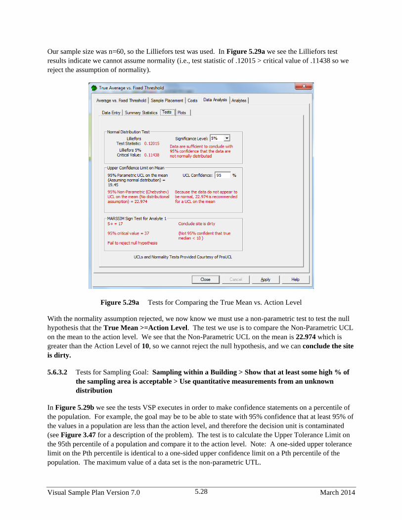
Visual Sample Plan Version 7.0 March 2014 5.28
Our sample size was n=60, so the Lilliefors test was used. In Figure 5.29a we see the Lilliefors test
results indicate we cannot assume normality (i.e., test statistic of .12015 > critical value of .11438 so we
reject the assumption of normality).
Figure 5.29a Tests for Comparing the True Mean vs. Action Level
With the normality assumption rejected, we now know we must use a non-parametric test to test the null
hypothesis that the True Mean >=Action Level. The test we use is to compare the Non-Parametric UCL
on the mean to the action level. We see that the Non-Parametric UCL on the mean is 22.974 which is
greater than the Action Level of 10, so we cannot reject the null hypothesis, and we can conclude the site
is dirty.
5.6.3.2 Tests for Sampling Goal: Sampling within a Building > Show that at least some high % of
the sampling area is acceptable > Use quantitative measurements from an unknown
distribution
In Figure 5.29b we see the tests VSP executes in order to make confidence statements on a percentile of
the population. For example, the goal may be to be able to state with 95% confidence that at least 95% of
the values in a population are less than the action level, and therefore the decision unit is contaminated
(see Figure 3.47 for a description of the problem). The test is to calculate the Upper Tolerance Limit on
the 95th percentile of a population and compare it to the action level. Note: A one-sided upper tolerance
limit on the Pth percentile is identical to a one-sided upper confidence limit on a Pth percentile of the
population. The maximum value of a data set is the non-parametric UTL.
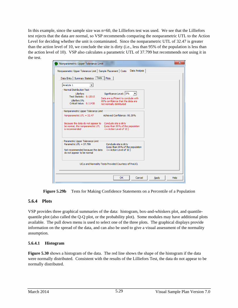
March 2014 Visual Sample Plan Version 7.0 5.29
In this example, since the sample size was n=60, the Lilliefors test was used. We see that the Lilliefors
test rejects that the data are normal, so VSP recommends comparing the nonparametric UTL to the Action
Level for deciding whether the unit is contaminated. Since the nonparametric UTL of 32.47 is greater
than the action level of 10, we conclude the site is dirty (i.e., less than 95% of the population is less than
the action level of 10). VSP also calculates a parametric UTL of 37.799 but recommends not using it in
the test.
Figure 5.29b Tests for Making Confidence Statements on a Percentile of a Population
5.6.4 Plots
VSP provides three graphical summaries of the data: histogram, box-and-whiskers plot, and quantile-
quantile plot (also called the Q-Q plot, or the probability plot). Some modules may have additional plots
available. The pull down menu is used to select one of the three plots. The graphical displays provide
information on the spread of the data, and can also be used to give a visual assessment of the normality
assumption.
5.6.4.1 Histogram
Figure 5.30 shows a histogram of the data. The red line shows the shape of the histogram if the data
were normally distributed. Consistent with the results of the Lilliefors Test, the data do not appear to be
normally distributed.

Visual Sample Plan Version 7.0 March 2014 5.30
Figure 5.30 Histogram of the data
5.6.4.2 Box-and-Whiskers Plot
Figure 5.31 shows a Box-and-Whiskers plot of the data. The Box-and-Whiskers plot is composed of a
central “box” divided by a line, and with two lines extending out from the box, called the “whiskers”.
The line through the box is drawn at the median of the data (i.e., the 50th percentile). The two ends of the
box represent the 25th and 75th percentiles of the data, also called the lower and upper quartiles of the data
set. The sample mean is shown as a red “+”. The upper whisker extends to the largest data value that is
less than the upper quartile plus 1.5 times the interquartile range (upper quartile – lower quartile). The
lower whisker extends to the smallest data value that is greater than the lower quartile minus 1.5 times the
interquartile range. Extreme data values (greater or smaller than the ends of the whiskers) are plotted
individually. If the data are normally distributed, the box and whiskers appear symmetrical, with the
median midway between the ends of the box (i.e., the 25th and 75th percentiles), and the mean is equal to
the median. The plot in Figure 5.31 is not symmetrical, consistent with the non-normality conclusion
discussed above.
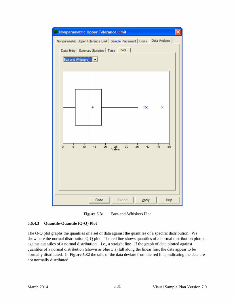
March 2014 Visual Sample Plan Version 7.0 5.31
Figure 5.31 Box-and-Whiskers Plot
5.6.4.3 Quantile-Quantile (Q-Q) Plot
The Q-Q plot graphs the quantiles of a set of data against the quantiles of a specific distribution. We
show here the normal distribution Q-Q plot. The red line shows quantiles of a normal distribution plotted
against quantiles of a normal distribution – i.e., a straight line. If the graph of data plotted against
quantiles of a normal distribution (shown as blue x’s) fall along the linear line, the data appear to be
normally distributed. In Figure 5.32 the tails of the data deviate from the red line, indicating the data are
not normally distributed.
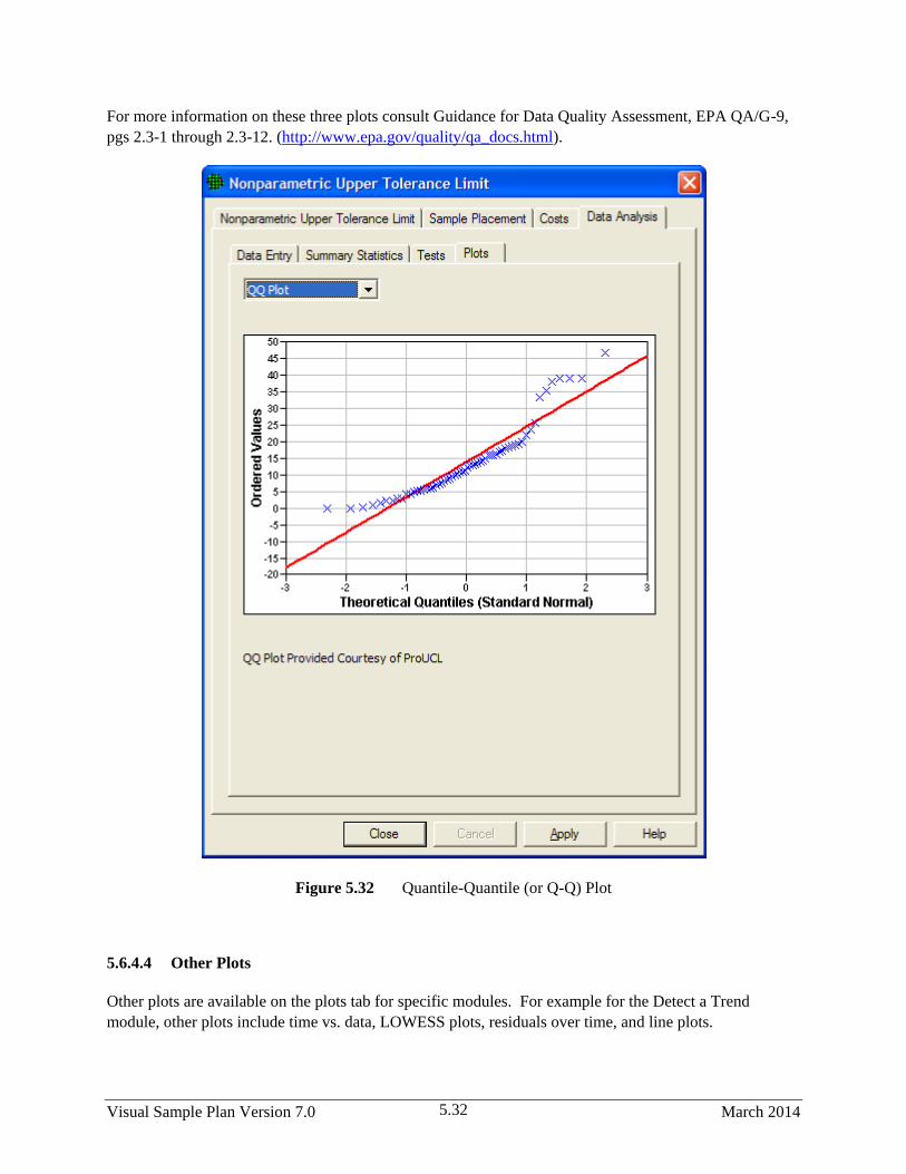
Visual Sample Plan Version 7.0 March 2014 5.32
For more information on these three plots consult Guidance for Data Quality Assessment, EPA QA/G-9,
pgs 2.3-1 through 2.3-12. (http://www.epa.gov/quality/qa_docs.html).
Figure 5.32 Quantile-Quantile (or Q-Q) Plot
5.6.4.4 Other Plots
Other plots are available on the plots tab for specific modules. For example for the Detect a Trend
module, other plots include time vs. data, LOWESS plots, residuals over time, and line plots.

March 2014 Visual Sample Plan Version 7.0 6.1
6.0 Room Features in VSP
VSP has a complete room supporting infrastructure, including sampling locations in 3 dimensions and a
local coordinate system. Under this system, a room in VSP is any Sample Area that has a height greater
than zero. The floor, walls and ceiling can be viewed in the Room View. Objects like doors and
windows can be placed in a room. Additional flat surfaces, called surface overlays, can also be placed in
the room to represent portions of a surface that need to be distinguished from the overall surface. Surface
overlays can also be elevated to represent the top surface of furniture. Samples can be placed on the
walls, ceiling, and surface overlays of a room as well as on the floor and on doors and windows. Samples
are placed on all selected rooms. To display the Room View, select View > Room from the main menu
or click on the Room View tool button on the main toolbar. Many of the VSP room features are
described in Section 2.5.1 Drawing a Room.
Some of the menu commands discussed in this chapter also have tool button shortcuts available on the
Room Toolbar. To activate the Room Toolbar, select View > Room Toolbar on the main menu.
6.1 Room Creation and Manipulation
6.1.1 Creating a Room from a Sample Area
Since a room in VSP is simply a sample area that has had its height set greater than zero, the simplest way
to create a room is to create a sample area and set its height to something like 8 feet. To set the height of
a room, right-click on the sample area on the map to display the Sample Area Information dialog box (see
Figure 6.1). The room height is one of the parameters that can be modified in this information dialog
box. The Room > Set Room Height menu command (or Set Height tool button) displays a dialog that
sets the height of all selected sample areas when the Map View is active, or sets the height of only the
current room when the Room View is active. (See Section 6.2.1 for a definition of current room.)
The Sample Area Information dialog also allows you to include or exclude the floor and the ceiling from
a room. These are included by default. If these surfaces are excluded they will not receive sample points
from any sampling design and they will not be displayed in the Room view.

Visual Sample Plan Version 7.0 March 2014 6.2
Figure 6.1 Sample Area Information Dialog
6.1.2 Drawing a Room
The Room > Draw menu command (or the Draw Room tool button) allows you to draw a room on the
map. Drawing a room is similar to drawing a rectangle, except that it automatically sets the wall height
for you. Define one corner of the floor rectangle by clicking on the map with the left mouse button or by
entering the coordinates on the keyboard (e.g., 100,200<Enter>). Then enter the opposite corner with the
mouse or keyboard. Holding the Ctrl key while clicking on the map limits the floor rectangle to a square.
An alternate method of defining a room is to enter the length, width, and height on the keyboard (Length
x Width x Height <Enter>). If the room is defined this way, then one corner is placed at the origin (0,0).
6.1.3 Room Delineation Method
If you have a building floor-plan map (such as a .dxf file from a CAD system), the Room Delineation
method is usually the fastest and easiest way to create rooms in VSP. Choosing Room > Delineate
Rooms from the menu (or clicking the Delineate Rooms tool button) toggles the room delineation mode
on or off. The room delineation mode allows you to create rooms with right angles inside existing map
shapes. This mode is for use in the map view. If a room contains some walls that are not at right angles
to other walls, those rooms will need to be created by the first method outlined in section 6.1.1.

March 2014 Visual Sample Plan Version 7.0 6.3
While in this mode, left-clicking with the mouse creates a red rectangle. The red rectangle is framed by
moving up, down, left and right from the point clicked and stopping at the first line encountered in that
direction. Several red rectangles may be needed to fill up the space inside an irregular shaped room on
the map.
After the room is filled with adjoining red rectangles, right-click with the mouse to combine all the
rectangles into a room. If there are disjoint red rectangles, each group of red rectangles becomes a
separate room. Figures 6.2a and 6.2b illustrates the delineation method in action.
If the desired room is a simple rectangle, right-click with the mouse to create the rectangle and convert it
to a room in a single step. Remember the red and black bulls-eye in the bottom left-hand corner of the
room in Figure 6.2b marks the location of the Room Origin for local coordinates (see Section 6.4.2).
6.1.4 Room Manipulation
The room can be modified in the map view by inserting a point into a wall and then moving the wall
section. To insert a new point into a wall, use the Map > Insert Point menu command. To move a wall
section, select the wall section by holding down the Shift key while clicking on the center of a wall
segment. Once selected, the wall segment can be dragged with the mouse. Hold the Ctrl key down while
dragging to the wall aligned at right angles. Figure 6.3 illustrates a new point inserted on the right side of
a room, the segment selected, and the segment being dragged outward.
You can also set the exact length of a selected wall segment by right-clicking on it. This displays a dialog
that allows you to change the length of the segment. Figure 6.4 illustrates a segment length being
changed with the dialog.

Visual Sample Plan Version 7.0 March 2014 6.4
Figure 6.2b. Room Delineation Mode
Figure 6.3. Room Manipulation
The On-line Help functions
provide more detailed
instructions on room
manipulation.
Figure 6.2a. Room Delineation Mode
Figure 6.4. Changing Segment Length

March 2014 Visual Sample Plan Version 7.0 6.5
6.2 Room Display Options
6.2.1 Current Room
When one or more rooms are
selected on a map, exactly one of
the rooms is the current room. The
current room is the one that is
displayed in the Room View. The
current room is also indicated on
the map by a thick black border and
a darker shade. The last room to be
created, selected, or viewed with
the Sample Information dialog
becomes the current room. Using
the Room > Next Room or Room
> Previous Room menu
commands scrolls through the list
of selected rooms. Each of these
commands also has a tool button.
Figure 6.5 shows the current room
in the Map View. Remember that
samples are placed on all selected sample areas/rooms, not just the current room. If you want to place
objects within a room, such as a door or a window, they can only be placed on the current room.
6.2.2 Room View Types
VSP provides 3 different room view types: perspective, wall-strip and splayed. These view types can be
selected using the menu commands:
Room > Perspective Room (or Perspective Room tool button)
Room > Room with Wall Strip (or Wall Strip Room tool button)
Room > Splayed Room (or Splayed Room tool button)
Figure 6.6. Room View Types
Figure 6.5. Current Room

Visual Sample Plan Version 7.0 March 2014 6.6
6.2.2.1 Perspective Room
The perspective room view shows the room as a 3-dimension semi-perspective view. Inside wall surfaces
that are facing you are displayed; inside wall surfaces that are facing away are not displayed. The floor is
shown tilted down and the ceiling (if included) is shown tilted up. The wall sections are shown attached
to the floor surface. (If the floor is excluded and the ceiling is included, then the wall sections are shown
attached to the ceiling surface.)
The Room > Rotate Room Left and Room > Rotate Room Right menu commands (or the Rotate Left
and Rotate Right tool buttons) rotate the room by 90 degrees, to allow viewing from a different
perspective. This does not change the coordinates of the room or any object associated with the room,
such as sample locations.
6.2.2.2 Wall-Strip Room
The wall strip room view shows a floor (if included), a mirror-image ceiling (if included), and a strip of
wall sections laid edge to edge. The floor and ceiling surfaces are shown attached to the proper wall
section.
The Room > Rotate Room Left and Room > Rotate Room Right menu commands (or the Rotate Left
and Rotate Right tool buttons) rotate the room by 90 degrees, to allow viewing the floor and ceiling from
different angles. This does not change the coordinates of the room or any object associated with the
room, such as sample locations.
6.2.2.3 Splayed Room
The splayed room view shows a floor, a mirror-image ceiling, and individual wall sections laid outward
from the floor. The wall sections are originally laid down so that they do not overlap. If the wall section
is not shown attached to the floor, a red line shows where it should be attached.
To move a wall section to a new location on the display, simply click and drag with the mouse. Right-
click with the mouse on a wall section to move it back to its attached location. Moving a wall section on
the display does not change the coordinates of the room or any object associated with the room, such as
sample locations.
6.2.3 Room North Arrow
By default, VSP places a north arrow on the room floor and ceiling surface. Figure 6.7 shows the north
arrows on the floor and ceiling. Use the View > Room North Arrow command to show or hide the north
arrow. The location of the north arrow can be changed by grabbing the center of the north arrow with the
mouse and dragging it. (The center to grab is between the N and the arrow.)
VSP assumes by default that north is the top of your map. If this is not the case, select the Map > Map
Settings menu command. Change the North Offset in the Map Extents dialog box to correct the direction
of north on your map.
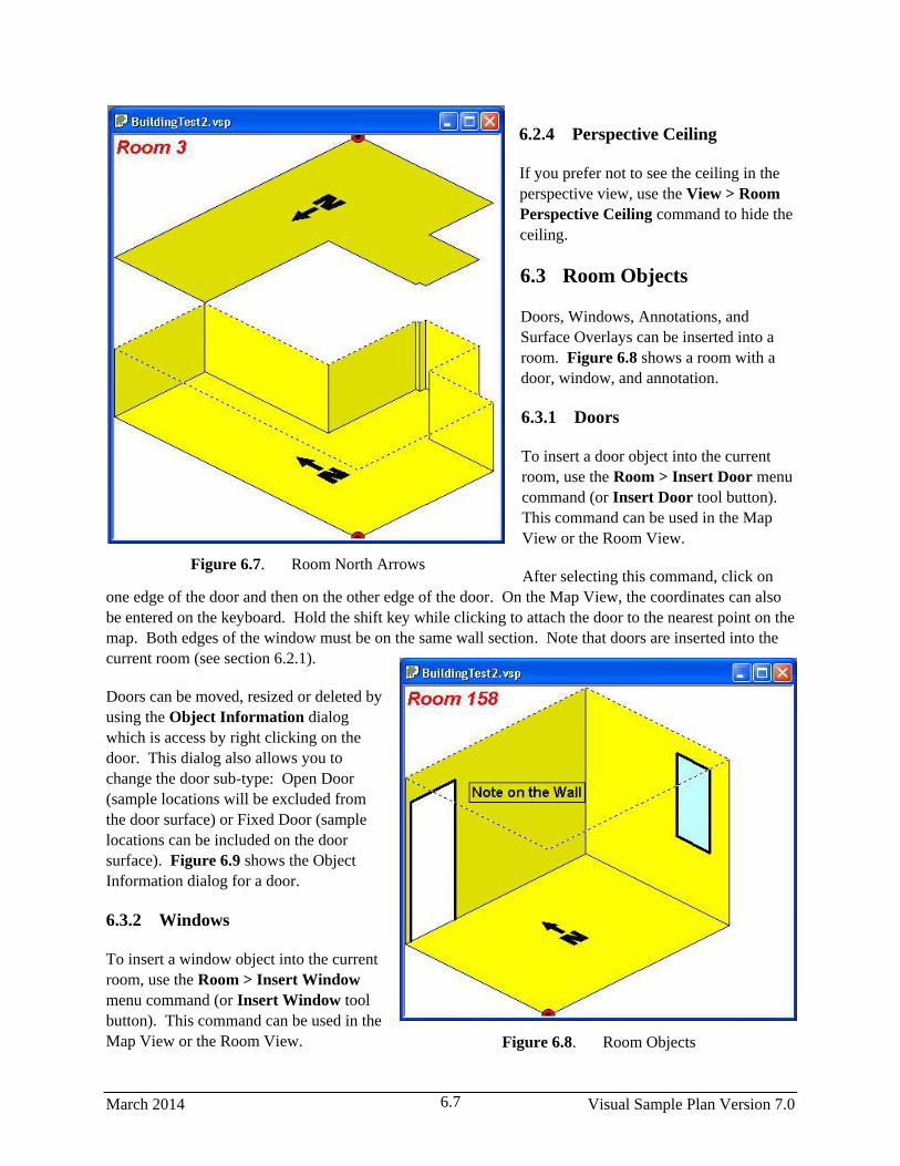
March 2014 Visual Sample Plan Version 7.0 6.7
Figure 6.7. Room North Arrows
Figure 6.8. Room Objects
6.2.4 Perspective Ceiling
If you prefer not to see the ceiling in the
perspective view, use the View > Room
Perspective Ceiling command to hide the
ceiling.
6.3 Room Objects
Doors, Windows, Annotations, and
Surface Overlays can be inserted into a
room. Figure 6.8 shows a room with a
door, window, and annotation.
6.3.1 Doors
To insert a door object into the current
room, use the Room > Insert Door menu
command (or Insert Door tool button).
This command can be used in the Map
View or the Room View.
After selecting this command, click on
one edge of the door and then on the other edge of the door. On the Map View, the coordinates can also
be entered on the keyboard. Hold the shift key while clicking to attach the door to the nearest point on the
map. Both edges of the window must be on the same wall section. Note that doors are inserted into the
current room (see section 6.2.1).
Doors can be moved, resized or deleted by
using the Object Information dialog
which is access by right clicking on the
door. This dialog also allows you to
change the door sub-type: Open Door
(sample locations will be excluded from
the door surface) or Fixed Door (sample
locations can be included on the door
surface). Figure 6.9 shows the Object
Information dialog for a door.
6.3.2 Windows
To insert a window object into the current
room, use the Room > Insert Window
menu command (or Insert Window tool
button). This command can be used in the
Map View or the Room View.
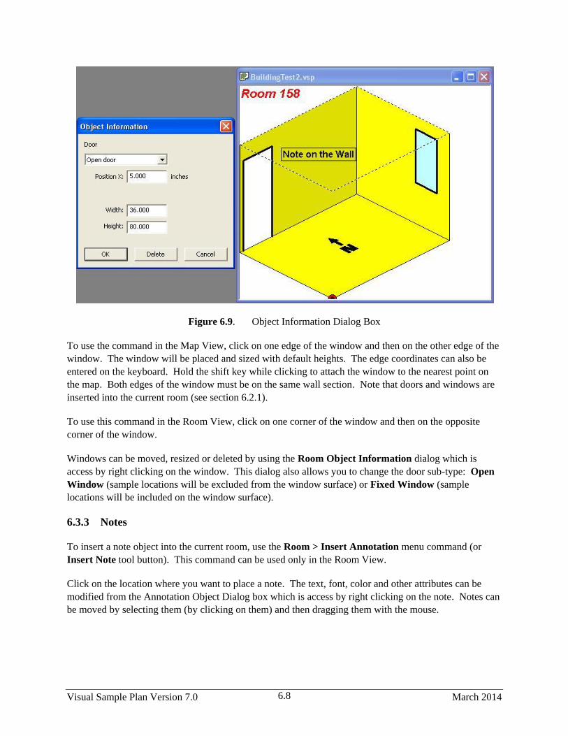
Visual Sample Plan Version 7.0 March 2014 6.8
Figure 6.9. Object Information Dialog Box
To use the command in the Map View, click on one edge of the window and then on the other edge of the
window. The window will be placed and sized with default heights. The edge coordinates can also be
entered on the keyboard. Hold the shift key while clicking to attach the window to the nearest point on
the map. Both edges of the window must be on the same wall section. Note that doors and windows are
inserted into the current room (see section 6.2.1).
To use this command in the Room View, click on one corner of the window and then on the opposite
corner of the window.
Windows can be moved, resized or deleted by using the Room Object Information dialog which is
access by right clicking on the window. This dialog also allows you to change the door sub-type: Open
Window (sample locations will be excluded from the window surface) or Fixed Window (sample
locations will be included on the window surface).
6.3.3 Notes
To insert a note object into the current room, use the Room > Insert Annotation menu command (or
Insert Note tool button). This command can be used only in the Room View.
Click on the location where you want to place a note. The text, font, color and other attributes can be
modified from the Annotation Object Dialog box which is access by right clicking on the note. Notes can
be moved by selecting them (by clicking on them) and then dragging them with the mouse.

March 2014 Visual Sample Plan Version 7.0 6.9
6.3.4 Surface Overlays
One or more surface overlays can be inserted in a room to represent a portion of a surface that needs to be
distinguished from the overall surface. For example, a portion of the floor in a room may be covered with
tile while most of the floor is covered with carpet, requiring a different sampling technique. A surface
overlay can be elevated from the floor to represent the top horizontal surface of a desk, chair, cabinet, or
shelf. Surface overlays can be placed on any surface in the room. Only floor overlays can be elevated.
To insert a surface overlay into the current room, use the Edit > Surfaces > Create Surface Overlay
menu command to bring up the surface overlay dialog box (Figure 6.10). This command can be used
only in the Room View (preferably the Perspective Room View). When initially placing a surface
overlay, this dialog box is simplified and the only option available is to choose a surface type. Choose the
Surface Type from the drop down menu (too add a new surface type, go to Edit > Surfaces > Surface
Types). Then click two opposite corners on the room’s floor. This will create a rectangular shaped box
on the room’s floor. Once a surface overlay is placed on a surface, right clicking on it brings up the more
extensive dialog box in Figure 6.10. Change this to an elevated surface changing the Height Above
Floor (and the sample placement parameters). An example of an elevated surface overlay is in Figure
6.11. Checking the “Allow samples on surface” box will allow sampling on the elevated surface when
sampling in the room. Checking “Allow samples on floor beneath surface” allows for sampling to occur
underneath the elevated surface. Similarly, checking “Allow samples on wall behind surface” allows for
sampling to occur on a section of a wall that a surface overlay is placed against.
Figure 6.10 . Surface Overlay Dialog
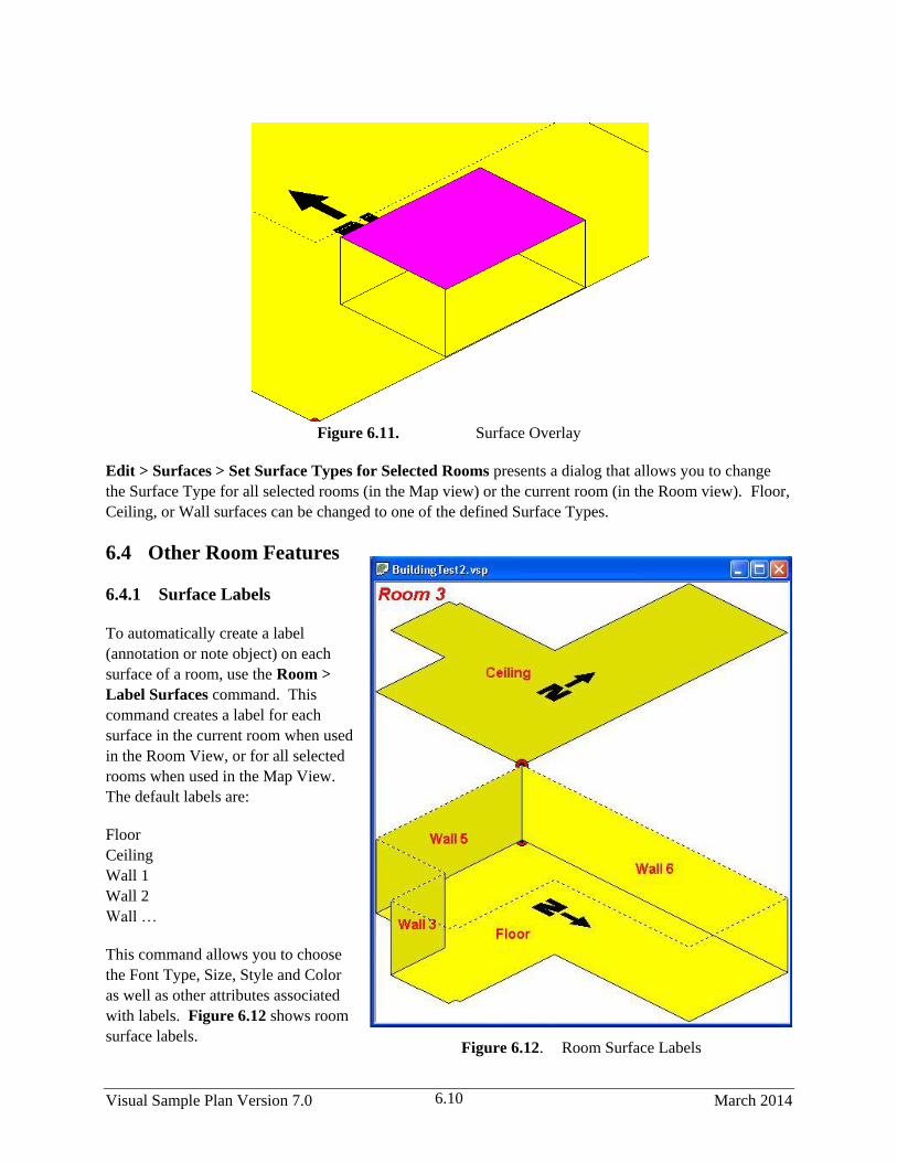
Visual Sample Plan Version 7.0 March 2014 6.10
Figure 6.12. Room Surface Labels
Figure 6.11. Surface Overlay
Edit > Surfaces > Set Surface Types for Selected Rooms presents a dialog that allows you to change
the Surface Type for all selected rooms (in the Map view) or the current room (in the Room view). Floor,
Ceiling, or Wall surfaces can be changed to one of the defined Surface Types.
6.4 Other Room Features
6.4.1 Surface Labels
To automatically create a label
(annotation or note object) on each
surface of a room, use the Room >
Label Surfaces command. This
command creates a label for each
surface in the current room when used
in the Room View, or for all selected
rooms when used in the Map View.
The default labels are:
Floor
Ceiling
Wall 1
Wall 2
Wall …
This command allows you to choose
the Font Type, Size, Style and Color
as well as other attributes associated
with labels. Figure 6.12 shows room
surface labels.

March 2014 Visual Sample Plan Version 7.0 6.11
After being created, the surface labels may be edited by right-clicking on them. If this command is run
again, it will delete any existing label surfaces and replace them with the default surface labels. The
surface label is also reported on the Sample Information dialog (accessed by right-clicking on a sample
location). Figure 6.13 shows a Sample Information dialog with a custom surface label.
6.4.2 Local Coordinates and Room Origin
VSP uses local coordinates to facilitate the location of samples inside of rooms (and also regular sample
areas). Local (LX, LY) are relative coordinates. Local coordinates can be viewed on the Sample
Information dialog in Figure 6.11.
In regular Sample Areas, the local coordinates are relative to the minimum X and minimum Y coordinates
of the sample area.
In Rooms, the local coordinates are relative to the surface they are on. For walls, the local coordinates are
relative to the lower left hand corner of the wall section as you are facing it. For the floor and ceiling, the
local coordinates are relative to the Room Origin. The location of Room Origin is shown on the Room
View by a red and black bull’s-eye.
Figure 6.13. Room Surface Labels
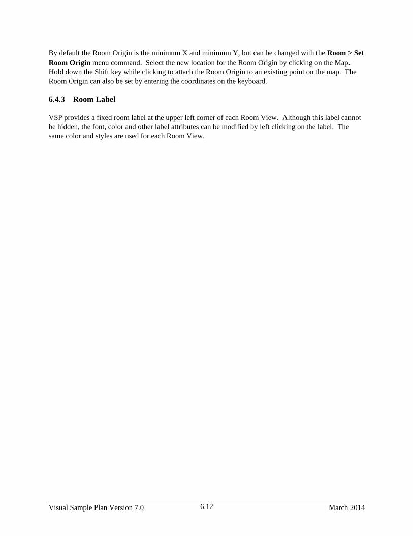
Visual Sample Plan Version 7.0 March 2014 6.12
By default the Room Origin is the minimum X and minimum Y, but can be changed with the Room > Set
Room Origin menu command. Select the new location for the Room Origin by clicking on the Map.
Hold down the Shift key while clicking to attach the Room Origin to an existing point on the map. The
Room Origin can also be set by entering the coordinates on the keyboard.
6.4.3 Room Label
VSP provides a fixed room label at the upper left corner of each Room View. Although this label cannot
be hidden, the font, color and other label attributes can be modified by left clicking on the label. The
same color and styles are used for each Room View.
March 2014 Visual Sample Plan Version 7.0 7.1
7.0 Unexploded Ordnance Site Related Modules and Features
VSP contains several tools for statistical site characterization protocols of sites potentially contaminated
with unexploded ordnance (UXO). These site characterization protocols help identify and delineate
potential target areas at a site using limited amounts of geophysical transect data (Hathaway 2008). Tools
include approaches for transect design, target identification, boundary delineation, and geophysical
anomaly density mapping.
7.1 Transect Spacing Needed to Locate Target Areas
Geophysical surveys are conducted at DoD sites and facilities to search for target areas at which
munitions were fired or dropped. Surface areas passed over by geophysical detectors, referred to as
transects, are usually up to several meters wide and run in a relatively straight line (as much as terrain
permits) from one point of a site to another. When a geophysical sensor system is deployed continuously
along transects, anomalies indicating munitions related items may be recorded. A goal of these surveys is
to identify areas of high anomaly density consistent with that of a target area. The transect design
methods in VSP are statistical approaches for determining the level of confidence in whether a transect
sampling design will traverse and/or detect a target area of a specific shape, size, and anomaly density.
Selecting Sampling Goals > Find Target Areas and Analyze Survey Results (UXO) > Transect
spacing needed to locate target areas accesses the VSP tools that calculate the probability that at least
one transect will traverse a target area of specified size and shape or estimate the probability the target
area will be traversed and detected with a specific transect design, assumed background density, and
target area density. In addition to these two methods, the user can manually place transects within a
sample area.
Table 7.1 lists the variables that can be adjusted in this dialog and identifies which transect design
method uses the variable. The three different methods are identified as Traversal, Traversal and
Detection, and Manual in Table 7.1. The “additional information” column provides general information
about the variable. Each of these variables will be described in more detail in the following sections. The
first four variables listed in the table (Transect Pattern, Transect Width, Target Area Shape, Target Area
Orientation) are generally defined by the survey equipment and the specific site use. The design objective
selected will determine the importance of the remaining variables. The design objectives are specifically
stated in VSP as “Ensure High Probability of Traversal Only” (traversal), “Ensure High Probability of
Traversal and Detection” (traversal and detection), and “Manual Transect Spacing” (manual).
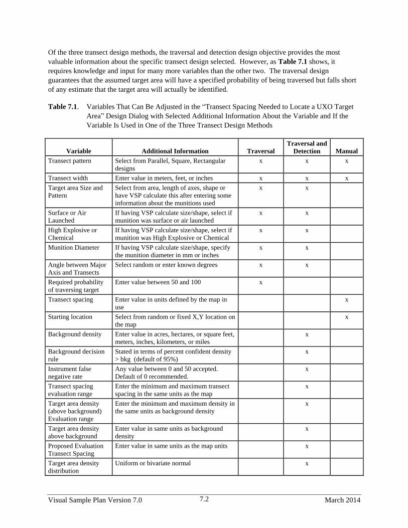
Visual Sample Plan Version 7.0 March 2014 7.2
Of the three transect design methods, the traversal and detection design objective provides the most
valuable information about the specific transect design selected. However, as Table 7.1 shows, it
requires knowledge and input for many more variables than the other two. The traversal design
guarantees that the assumed target area will have a specified probability of being traversed but falls short
of any estimate that the target area will actually be identified.
Table 7.1. Variables That Can Be Adjusted in the “Transect Spacing Needed to Locate a UXO Target
Area” Design Dialog with Selected Additional Information About the Variable and If the
Variable Is Used in One of the Three Transect Design Methods
Variable Additional Information Traversal
Traversal and
Detection Manual
Transect pattern Select from Parallel, Square, Rectangular
designs
x x x
Transect width Enter value in meters, feet, or inches x x x
Target area Size and
Pattern
Select from area, length of axes, shape or
have VSP calculate this after entering some
information about the munitions used
x x
Surface or Air
Launched
If having VSP calculate size/shape, select if
munition was surface or air launched
x x
High Explosive or
Chemical
If having VSP calculate size/shape, select if
munition was High Explosive or Chemical
x x
Munition Diameter If having VSP calculate size/shape, specify
the munition diameter in mm or inches
x x
Angle between Major
Axis and Transects
Select random or enter known degrees x x
Required probability
of traversing target
Enter value between 50 and 100 x
Transect spacing Enter value in units defined by the map in
use
x
Starting location Select from random or fixed X,Y location on
the map
x
Background density Enter value in acres, hectares, or square feet,
meters, inches, kilometers, or miles
x
Background decision
rule
Stated in terms of percent confident density
> bkg (default of 95%)
x
Instrument false
negative rate
Any value between 0 and 50 accepted.
Default of 0 recommended.
x
Transect spacing
evaluation range
Enter the minimum and maximum transect
spacing in the same units as the map
x
Target area density
(above background)
Evaluation range
Enter the minimum and maximum density in
the same units as background density
x
Target area density
above background
Enter value in same units as background
density
x
Proposed Evaluation
Transect Spacing
Enter value in same units as the map units x
Target area density
distribution
Uniform or bivariate normal x

March 2014 Visual Sample Plan Version 7.0 7.3
Density input Used only for the bivariate normal target
area density distribution. Select outer edge,
center, or average of the target area
x
Minimum precision A proportion between 0.05 and 0.20 x
Maximum error A proportion between 0.005 and 0.10 x
Search window
diameter
Enter value in units defined by the map in
use
x
7.1.1 Survey and Target Area Pattern
The “Survey and Target Area Pattern” tab shown in Figure 7.1 is used to enter information about the
transect pattern of interest, the transect width (width of the area covered by the geophysical detector), the
size and shape of the target area, and the angle between the major axis of the target area and the transects.
Figure 7.1. Survey and Target Area Pattern Tab
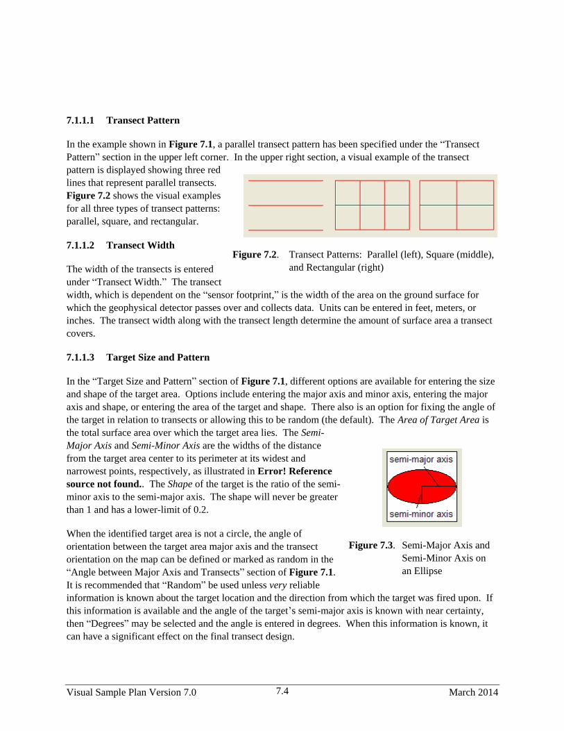
Visual Sample Plan Version 7.0 March 2014 7.4
7.1.1.1 Transect Pattern
In the example shown in Figure 7.1, a parallel transect pattern has been specified under the “Transect
Pattern” section in the upper left corner. In the upper right section, a visual example of the transect
pattern is displayed showing three red
lines that represent parallel transects.
Figure 7.2 shows the visual examples
for all three types of transect patterns:
parallel, square, and rectangular.
7.1.1.2 Transect Width
The width of the transects is entered
under “Transect Width.” The transect
width, which is dependent on the “sensor footprint,” is the width of the area on the ground surface for
which the geophysical detector passes over and collects data. Units can be entered in feet, meters, or
inches. The transect width along with the transect length determine the amount of surface area a transect
covers.
7.1.1.3 Target Size and Pattern
In the “Target Size and Pattern” section of Figure 7.1, different options are available for entering the size
and shape of the target area. Options include entering the major axis and minor axis, entering the major
axis and shape, or entering the area of the target and shape. There also is an option for fixing the angle of
the target in relation to transects or allowing this to be random (the default). The Area of Target Area is
the total surface area over which the target area lies. The Semi-
Major Axis and Semi-Minor Axis are the widths of the distance
from the target area center to its perimeter at its widest and
narrowest points, respectively, as illustrated in Error! Reference
source not found.. The Shape of the target is the ratio of the semi-
minor axis to the semi-major axis. The shape will never be greater
than 1 and has a lower-limit of 0.2.
When the identified target area is not a circle, the angle of
orientation between the target area major axis and the transect
orientation on the map can be defined or marked as random in the
“Angle between Major Axis and Transects” section of Figure 7.1.
It is recommended that “Random” be used unless very reliable
information is known about the target location and the direction from which the target was fired upon. If
this information is available and the angle of the target’s semi-major axis is known with near certainty,
then “Degrees” may be selected and the angle is entered in degrees. When this information is known, it
can have a significant effect on the final transect design.
Figure 7.2. Transect Patterns: Parallel (left), Square (middle),
and Rectangular (right)
Figure 7.3. Semi-Major Axis and
Semi-Minor Axis on
an Ellipse

March 2014 Visual Sample Plan Version 7.0 7.5
There is also an option “I want VSP to calculate the size/shape of the target areas of concern.” This is
shown in Figure 7.4. If information is known about the type of munition used, this can be entered, and
VSP can recommend a target area size and shape based on historical information.
Figure 7.4. Having VSP Calculate the Size/Shape of the Target Area
7.1.2 Transect Spacing
The “Transect Spacing” tab shown in Figure 7.5 is used to enter information about the design objective
and parameters needed to assess those objectives other than those covered in the “Survey and Target
Area” tab.
.
Figure 7.5. Transect Spacing Tab for Design Objective “Ensure High Probability of Traversal and
Detection” and “Transect Spacing Evaluation Range”

Visual Sample Plan Version 7.0 March 2014 7.6
7.1.2.1 Design Objective
There are three design objectives to choose from: 1) Ensure high probability of traversal and detection, 2)
Ensure high probability of traversal only, and 3) Manual transect spacing. Each of these design objectives
and their required parameters are explained in Sections 7.1.2.1.1 through 7.1.2.1.3.
Figure 7.5 shows the Transect Spacing tab when “Ensure high probability of traversal and detection” is
selected as the Design Objective and “transect spacing evaluation range” is selected from the drop-down
menu under Target Detection Performance. Figure 7.5 shows the Transect Spacing tab for the same
Design Objective for when “TA density (above background) range” is selected from the drop-down
menu.
Figure 7.6. Transect Spacing Tab for Design Objective “Ensure High Probability of Traversal and
Detection” and “TA Density (above background) Range”
The Background Density of a site is the expected density in an area where anomalies occur solely from
geologic material or anthropogenic clutter not related to DoD range activities. These background
anomalies are distributed with a consistent background rate throughout the site. Areas containing UXO
and other munitions-related anomalies are expected to have density greater than background.

March 2014 Visual Sample Plan Version 7.0 7.7
The Decision Rule is the required percent confidence that an area has density greater than background
density needed to conclude it is an area of interest. VSP evaluates a number of “windows,” which are
circular areas centered along transects. The Decision Rule refers to the percent confidence for an
individual window. VSP will “flag” an area that appears to have density higher than background density
according to the decision rule. An area is flagged if the actual density is significantly higher than the
expected background density. In statistical terms, the decision rule is 1 – α expressed as a percentage,
where α is the probability of a type I error, or the probability of concluding an area has density greater
than background when it is truly a background area.
The Instrument False Negative Rate accounts for the fact that collected data may not be representative of
the actual density because the geophysical detector may not identify all detectable anomalies. For
example, a false negative rate of 5% would indicate the detector, on average, would fail to detect 5% of
the detectable anomalies traversed (background and target area). It is generally assumed that the detector
always detects individual anomalies of interest, thus a false negative rate of 0% is used for a default value.
Min and Max refer to a range of transect spacings or target area anomaly densities (above background) to
evaluate. When the design objective is Ensure high probability of traversal and detection, the user has
the option of choosing to produce a TA density (above background) range or a transect spacing evalu-
ation range. When working with a transect spacing evaluation range, users must enter the Min
(minimum) and Max (maximum) transect spacings they want to consider. For rectangular transect
patterns, this refers to the set of transects with the more narrow transect spacing. Thus, if a user wants to
evaluate a range of transect spacings, he would enter this range as the Min and Max. VSP will evaluate
the transect spacings Min and Max in addition to spacings between those values. When TA density (above
background) range is chosen, Min and Max refer to the target area density above background. VSP will
evaluate a range of target area densities above background to estimate how well the transect design will
detect the target depending on the anomaly density of that target.
The Expected Target Area Density Above Background in Figure 7.5 is the anomaly density of the target
(excluding background density) when transect spacing evaluation range is selected. To evaluate a range
of transect spacings, the anomaly density of the target remains fixed.
The Proposed Evaluation Transect Spacing in Figure 7.6 is the transect spacing to use when TA density
(above background) range is selected. To evaluate a range of target densities, the transect spacing
remains fixed. Selecting the Graph Additional Detection Curves box works as described in the following
paragraph with density and transect spacing interchanged.
Checking the Graph Additional Detection Curves box will produce two additional curves on the graph for
the density or transect spacing specified. The additional curves will be for one half and twice the fixed
input variable. This allows for the examination of the sensitivity of both changes in transect spacings and
changes in target density on the same graph. Because this requires additional simulations for the
additional curves, this option increases the simulation run time by a factor of 3.
The Graph Options button brings up the additional dialog in Figure 7.7.
The user can choose between a Uniform Density and a Bivariate Normal Density for the distribution of
anomalies, excluding background, within the target area. If Uniform Density is chosen, the distribution of
anomalies within the target area is assumed to be randomly distributed throughout the entire target area.

Visual Sample Plan Version 7.0 March 2014 7.8
If Bivariate Normal Density is chosen, the distribution of anomalies within the TA is assumed to be
biased toward higher densities in the center of the TA such that the densities from the TA center to the TA
perimeter follow an approximately normal curve.
Average Target Area Density (above
background) defines how the density
value inputs for the Bivariate Normal
Density are entered when selected
(this option is disabled when Uniform
Density is selected). The default is
that target area densities are entered
as the Target Average, or average
anomaly density (above background)
of the target. Also available are
Outer Edge of Target and Center of
Target, which refer to the density
near the perimeter of the target area
and the center of the target area,
respectively. Changing to one of
these options will allow the user to
enter target area densities for the
target edge or center instead of the
target area average anomaly density.
Min (Minimum) Precision is used to determine the number of different TA densities or transect spacings
to simulate. Decreasing the Min Precision typically requires more transect spacings or densities to be
simulated and increases the length of the simulation. Increasing the Min Precision will typically decrease
the length of the simulation.
Max (Maximum) Error determines the number of iterations for each transect spacing or density
simulated. Decreasing the Max Error requires more simulations for each transect spacing or density
simulated and increases the overall simulation time. Increasing the Max Error will decrease the
simulation time.
The Search Window Diameter refers to the diameter of the
circular search window used to identify areas in which
density is greater than background density. The window is
actually a moving window that moves in increments of one-
sixth the window diameter along each transect, as shown in
Figure 7.8. Each search window is evaluated to determine if
the density is significantly greater than background density.
VSP calculates a default window diameter for the current
design, but checking the Override box allows the user to
manually enter a window diameter. The Critical Number of
Anomalies refers to the number of detected anomalies
required inside a window to identify it as significantly
greater than background.
Figure 7.7. Graph Options
Figure 7.8. Example of Windows
Moving Along the Center
Transect Shown

March 2014 Visual Sample Plan Version 7.0 7.9
Checking the Show this dialog each time graph is created has the dialog box in Figure 7.7 appear after
pressing the Create Graph button (Figure 7.5 and Figure 7.6) but before simulations are run and a graph
is produced. Otherwise, pressing the Create Graph button will skip this step and proceed with running
simulations followed by producing a graph.
An example of the resulting graph, or power curve, for this tool is shown in Figure 7.9, where Transect
spacing evaluation range was selected and the Graph Additional Detection Curves box was checked.
This graph shows the effectiveness of a range of transect spacings for detecting the target area. It also
shows the sensitivity of detecting the target area for different target area densities.
Figure 7.9. Power Curve with Transect Spacing as the X-Axis and Additional Curves Displayed
Figure 7.10 shows the Transect Spacing tab when “Ensure high probability of traversal only” is selected
as the Design Objective. A subset of the parameters used for “Ensure high probability of traversal and
detection” is used for this dialog with one new parameter, Required Probability of Traversing the Target.
This is the required probability the design chosen will traverse the target area. VSP calculates the transect
spacing required to achieve this probability and displays the result in red text. Definitions for the other
parameters are the same as those in Section 7.1.2.1.1. These parameters allow the user to specify the
Target Area Density Evaluation Range to examine how well the transect design will detect the target area
for different target area densities.

Visual Sample Plan Version 7.0 March 2014 7.10
Figure 7.10. Transect Spacing Tab for Design Objective “Ensure High Probability of Traversal Only”
Figure 7.11 shows the Transect Spacing tab when “Manual transect spacing” is selected as the Design
Objective. This option makes available some of VSP’s useful features without using data quality
objectives. Before deciding to develop a sampling plan based on a user-supplied transect spacing and
starting location, consider the assumptions and limitations involved.

March 2014 Visual Sample Plan Version 7.0 7.11
Figure 7.11. Transect Spacing Tab for Design Objective “Manual Transect Spacing”
7.1.3 Costs
The Cost tab provides an estimate of costs using the chosen transect design on the current VSP map. The
user must enter the Fixed Planning and Validation Costs, Setup Cost per Transect, and Collection Cost
per Linear Unit to calculate the Total Cost of Transect Sampling.
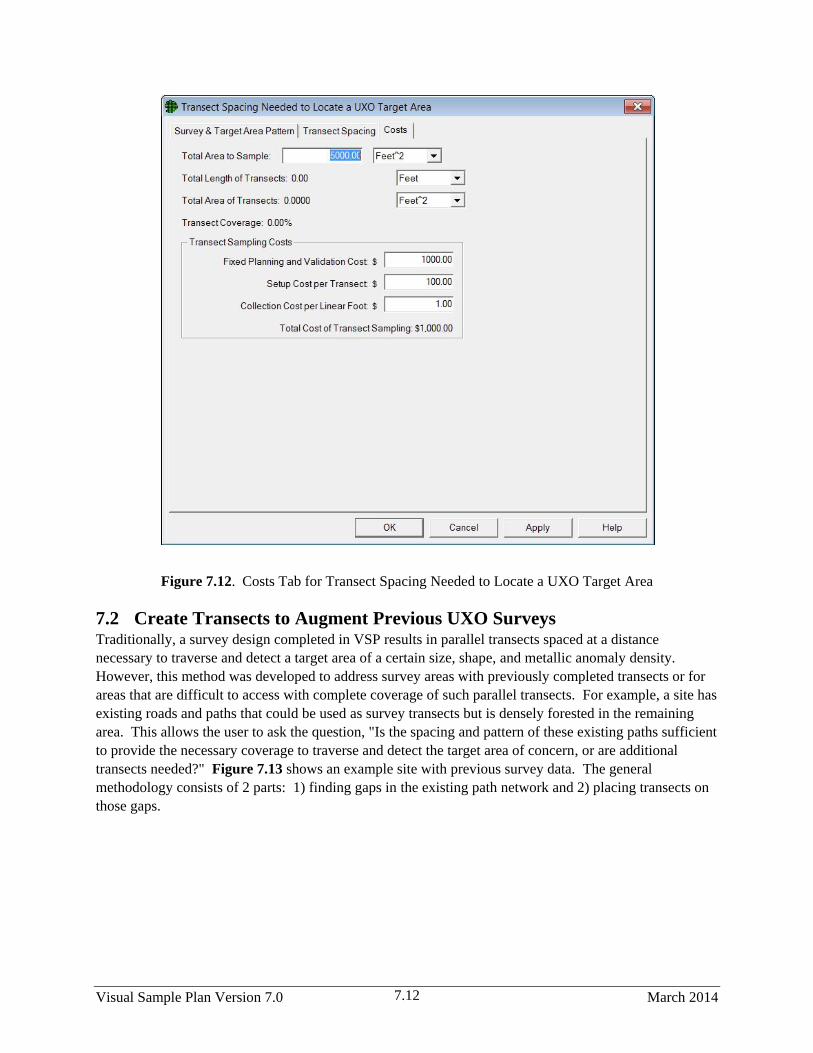
Visual Sample Plan Version 7.0 March 2014 7.12
Figure 7.12. Costs Tab for Transect Spacing Needed to Locate a UXO Target Area
7.2 Create Transects to Augment Previous UXO Surveys Traditionally, a survey design completed in VSP results in parallel transects spaced at a distance
necessary to traverse and detect a target area of a certain size, shape, and metallic anomaly density.
However, this method was developed to address survey areas with previously completed transects or for
areas that are difficult to access with complete coverage of such parallel transects. For example, a site has
existing roads and paths that could be used as survey transects but is densely forested in the remaining
area. This allows the user to ask the question, "Is the spacing and pattern of these existing paths sufficient
to provide the necessary coverage to traverse and detect the target area of concern, or are additional
transects needed?" Figure 7.13 shows an example site with previous survey data. The general
methodology consists of 2 parts: 1) finding gaps in the existing path network and 2) placing transects on
those gaps.

March 2014 Visual Sample Plan Version 7.0 7.13
Figure 7.13. Example Site that Contains Surveys Along Existing Roads and Paths
Figure 7.14 shows the Gaps & New Transects tab of the dialogue for this module. The Survey & Target
Area Pattern tab and the Transect Spacing tab are similar to the tabs described in Sections 7.1.1 and 7.1.2
and deal with setting the same parameters above transect width, target area shape and size, and transect
spacing. There are no parameters in the these tabs not covered in Sections 7.1.1 and 7.1.2, and therefore
referring to those sections will described the parameters used in this module.

Visual Sample Plan Version 7.0 March 2014 7.14
Figure 7.14. Survey & Target Area Pattern Tab
In the Gaps & New Transects tab shown in Figure 7.14, the “Buffer around previous transects” tells VSP
not to augment portions of the sample area within this distance of already existing transects. The default
for this is the transect spacing selected on the Transect Spacing tab. Existing course-over-ground (COG)
data is imported by clicking on “Import” and selecting the relevant files. Once the data is imported, the
gaps in the existing path network are found by clicking “Find Gaps”. The number of gaps and some
summary information about the various sizes of the gaps are shown. Figure 7.15 shows the map from
Figure 7.13 with the gaps found colored in green.

March 2014 Visual Sample Plan Version 7.0 7.15
Figure 7.15. Gaps Left by Putting a Buffer Around the Existing Paths
Once gaps have been found, the next step is to place transects on those gaps. Some options at the bottom
of the Gaps & New Transects tab include “Connect transects together”, which will create long continuous
paths, and “Attach transects to existing paths”. Once a decision is made on whether to use these options,
new transects are placed by clicking “Apply”. Parallel transects are placed in gap areas while trying to
minimize the total length of the transects in order to traverse potential target areas that would have been
missed by transects on existing paths. You can choose the option of having transects connected together
into long continuous paths. Another option is to have the new transect paths attached to existing paths.
The site previously shown with newly placed transects is shown in Figure 7.16.

Visual Sample Plan Version 7.0 March 2014 7.16
Figure 7.16. Parallel Transects Placed on the Gaps, Connected Together and Attached to Existing Paths
7.3 Locate and Mark UXO Target Areas Based on Elevated Anomaly
Density
Once a transect design has been accepted and the geophysical survey completed, the surveyed data (i.e.,
the transect course-over-ground and anomaly location data) is imported into VSP and analyzed. This
process is begun in VSP by selecting Sampling Goals > Find Target Areas and Analyze Survey
Results (UXO) > Locate and mark target areas based on elevated anomaly density. Section 7.3.1
details how these data can be imported and manipulated in VSP. Section 7.3.2 describes the methods
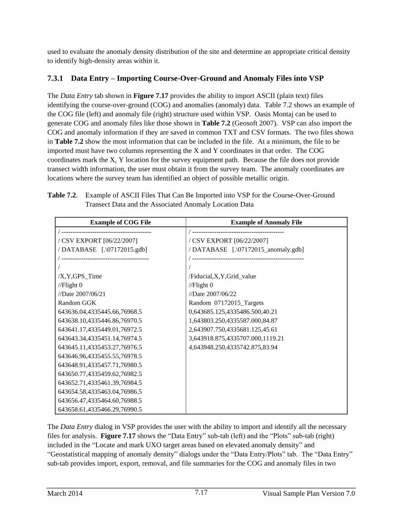
March 2014 Visual Sample Plan Version 7.0 7.17
used to evaluate the anomaly density distribution of the site and determine an appropriate critical density
to identify high-density areas within it.
7.3.1 Data Entry – Importing Course-Over-Ground and Anomaly Files into VSP
The Data Entry tab shown in Figure 7.17 provides the ability to import ASCII (plain text) files
identifying the course-over-ground (COG) and anomalies (anomaly) data. Table 7.2 shows an example of
the COG file (left) and anomaly file (right) structure used within VSP. Oasis Montaj can be used to
generate COG and anomaly files like those shown in Table 7.2 (Geosoft 2007). VSP can also import the
COG and anomaly information if they are saved in common TXT and CSV formats. The two files shown
in Table 7.2 show the most information that can be included in the file. At a minimum, the file to be
imported must have two columns representing the X and Y coordinates in that order. The COG
coordinates mark the X, Y location for the survey equipment path. Because the file does not provide
transect width information, the user must obtain it from the survey team. The anomaly coordinates are
locations where the survey team has identified an object of possible metallic origin.
Table 7.2. Example of ASCII Files That Can Be Imported into VSP for the Course-Over-Ground
Transect Data and the Associated Anomaly Location Data
Example of COG File Example of Anomaly File
/ ----------------------------------------- / ------------------------------------------
/ CSV EXPORT [06/22/2007] / CSV EXPORT [06/22/2007]
/ DATABASE [.\07172015.gdb] / DATABASE [.\07172015_anomaly.gdb]
/ ---------------------------------------- / ---------------------------------------------------
/ /
/X,Y,GPS_Time /Fiducial,X,Y,Grid_value
//Flight 0 //Flight 0
//Date 2007/06/21 //Date 2007/06/22
Random GGK Random 07172015_Targets
643636.04,4335445.66,76968.5 0,643685.125,4335486.500,40.21
643638.10,4335446.86,76970.5 1,643803.250,4335587.000,84.87
643641.17,4335449.01,76972.5 2,643907.750,4335681.125,45.61
643643.34,4335451.14,76974.5 3,643918.875,4335707.000,1119.21
643645.11,4335453.27,76976.5 4,643948.250,4335742.875,83.94
643646.96,4335455.55,76978.5
643648.91,4335457.71,76980.5
643650.77,4335459.62,76982.5
643652.71,4335461.39,76984.5
643654.58,4335463.04,76986.5
643656.47,4335464.60,76988.5
643658.61,4335466.29,76990.5
The Data Entry dialog in VSP provides the user with the ability to import and identify all the necessary
files for analysis. Figure 7.17 shows the “Data Entry” sub-tab (left) and the “Plots” sub-tab (right)
included in the “Locate and mark UXO target areas based on elevated anomaly density” and
“Geostatistical mapping of anomaly density” dialogs under the “Data Entry/Plots” tab. The “Data Entry”
sub-tab provides import, export, removal, and file summaries for the COG and anomaly files in two
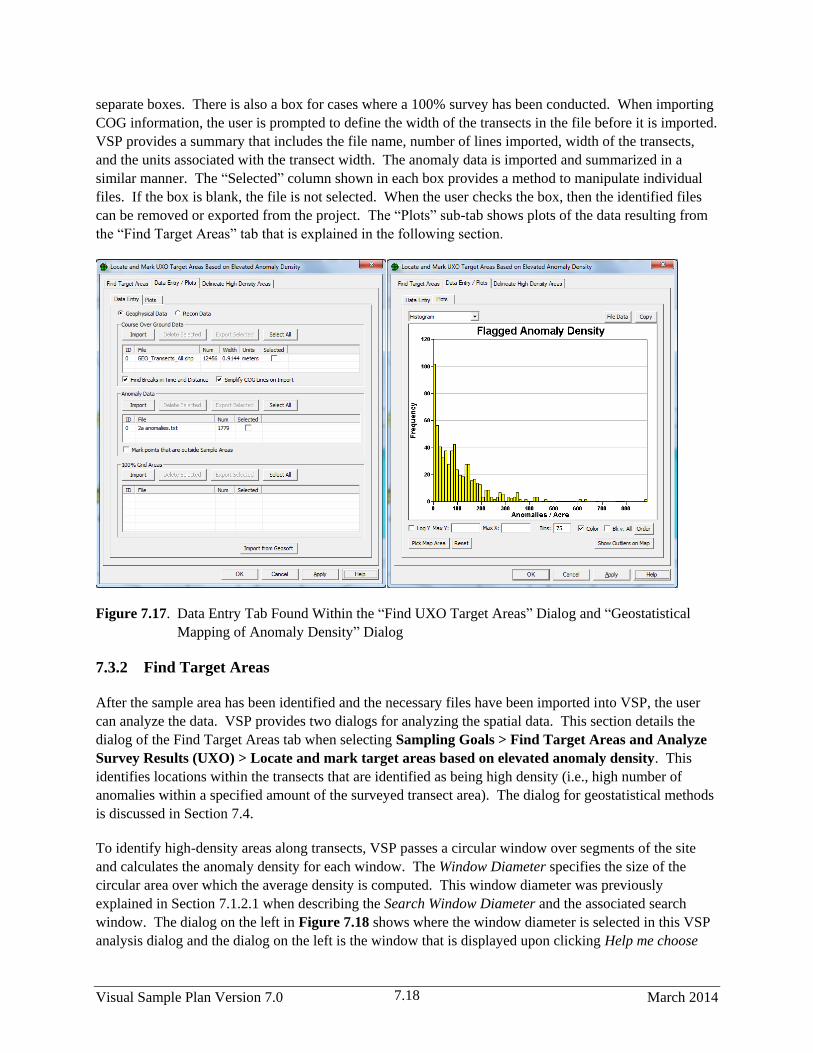
Visual Sample Plan Version 7.0 March 2014 7.18
separate boxes. There is also a box for cases where a 100% survey has been conducted. When importing
COG information, the user is prompted to define the width of the transects in the file before it is imported.
VSP provides a summary that includes the file name, number of lines imported, width of the transects,
and the units associated with the transect width. The anomaly data is imported and summarized in a
similar manner. The “Selected” column shown in each box provides a method to manipulate individual
files. If the box is blank, the file is not selected. When the user checks the box, then the identified files
can be removed or exported from the project. The “Plots” sub-tab shows plots of the data resulting from
the “Find Target Areas” tab that is explained in the following section.
Figure 7.17. Data Entry Tab Found Within the “Find UXO Target Areas” Dialog and “Geostatistical
Mapping of Anomaly Density” Dialog
7.3.2 Find Target Areas
After the sample area has been identified and the necessary files have been imported into VSP, the user
can analyze the data. VSP provides two dialogs for analyzing the spatial data. This section details the
dialog of the Find Target Areas tab when selecting Sampling Goals > Find Target Areas and Analyze
Survey Results (UXO) > Locate and mark target areas based on elevated anomaly density. This
identifies locations within the transects that are identified as being high density (i.e., high number of
anomalies within a specified amount of the surveyed transect area). The dialog for geostatistical methods
is discussed in Section 7.4.
To identify high-density areas along transects, VSP passes a circular window over segments of the site
and calculates the anomaly density for each window. The Window Diameter specifies the size of the
circular area over which the average density is computed. This window diameter was previously
explained in Section 7.1.2.1 when describing the Search Window Diameter and the associated search
window. The dialog on the left in Figure 7.18 shows where the window diameter is selected in this VSP
analysis dialog and the dialog on the left is the window that is displayed upon clicking Help me choose

March 2014 Visual Sample Plan Version 7.0 7.19
window size that can be used to provide a visual evaluation of appropriate window sizes which will be
explained in more detail later in this section. Figure 7.19 provides an example of how the window
diameter is used to calculate transect grid densities. The window diameter defines the size of a centered
circular window (orange and blue circles in Figure 7.19), which moves every one-sixth the selected
diameter and uses the anomaly count with the transect area within the window to calculate a density
assigned to the central transect grid (orange and blue boxes in Figure 7.19) centered in the window. The
green dots in Figure 7.19 represent the identified anomalies within the two surveyed transects. For
transects with length less than one-sixth the window diameter, such as in course-over-ground data, the
window may step over several transects.
Figure 7.18. Find Target Areas tab when “Flag Areas with Density Significantly > critical density” is
selected (left) and the results from using the “Window Size Sensitivity” dialog (right) that
appears when pressing the button Help me choose window size.
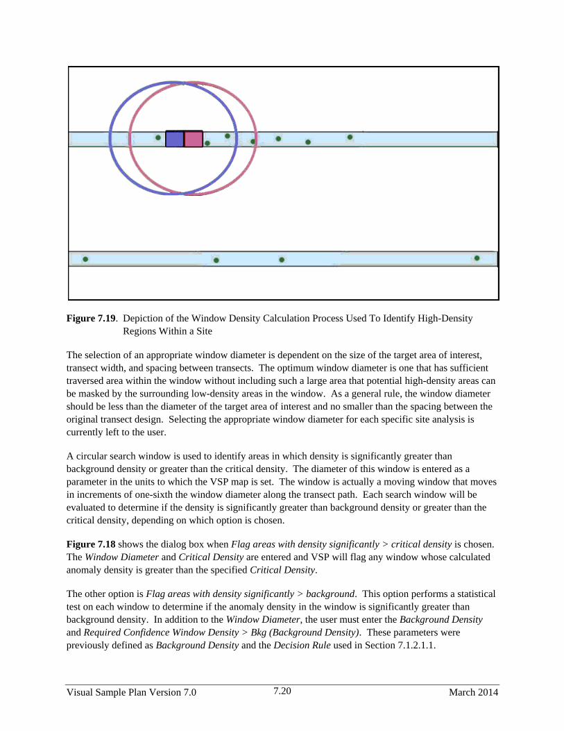
Visual Sample Plan Version 7.0 March 2014 7.20
Figure 7.19. Depiction of the Window Density Calculation Process Used To Identify High-Density
Regions Within a Site
The selection of an appropriate window diameter is dependent on the size of the target area of interest,
transect width, and spacing between transects. The optimum window diameter is one that has sufficient
traversed area within the window without including such a large area that potential high-density areas can
be masked by the surrounding low-density areas in the window. As a general rule, the window diameter
should be less than the diameter of the target area of interest and no smaller than the spacing between the
original transect design. Selecting the appropriate window diameter for each specific site analysis is
currently left to the user.
A circular search window is used to identify areas in which density is significantly greater than
background density or greater than the critical density. The diameter of this window is entered as a
parameter in the units to which the VSP map is set. The window is actually a moving window that moves
in increments of one-sixth the window diameter along the transect path. Each search window will be
evaluated to determine if the density is significantly greater than background density or greater than the
critical density, depending on which option is chosen.
Figure 7.18 shows the dialog box when Flag areas with density significantly > critical density is chosen.
The Window Diameter and Critical Density are entered and VSP will flag any window whose calculated
anomaly density is greater than the specified Critical Density.
The other option is Flag areas with density significantly > background. This option performs a statistical
test on each window to determine if the anomaly density in the window is significantly greater than
background density. In addition to the Window Diameter, the user must enter the Background Density
and Required Confidence Window Density > Bkg (Background Density). These parameters were
previously defined as Background Density and the Decision Rule used in Section 7.1.2.1.1.
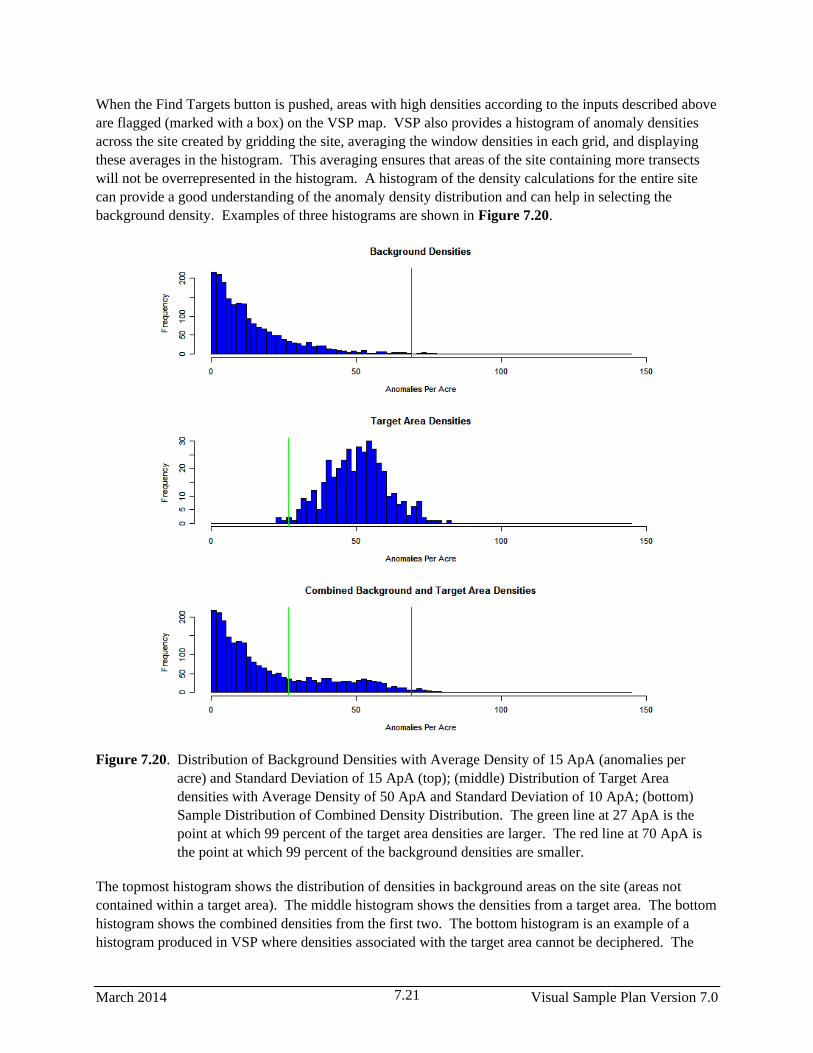
March 2014 Visual Sample Plan Version 7.0 7.21
When the Find Targets button is pushed, areas with high densities according to the inputs described above
are flagged (marked with a box) on the VSP map. VSP also provides a histogram of anomaly densities
across the site created by gridding the site, averaging the window densities in each grid, and displaying
these averages in the histogram. This averaging ensures that areas of the site containing more transects
will not be overrepresented in the histogram. A histogram of the density calculations for the entire site
can provide a good understanding of the anomaly density distribution and can help in selecting the
background density. Examples of three histograms are shown in Figure 7.20.
Figure 7.20. Distribution of Background Densities with Average Density of 15 ApA (anomalies per
acre) and Standard Deviation of 15 ApA (top); (middle) Distribution of Target Area
densities with Average Density of 50 ApA and Standard Deviation of 10 ApA; (bottom)
Sample Distribution of Combined Density Distribution. The green line at 27 ApA is the
point at which 99 percent of the target area densities are larger. The red line at 70 ApA is
the point at which 99 percent of the background densities are smaller.
The topmost histogram shows the distribution of densities in background areas on the site (areas not
contained within a target area). The middle histogram shows the densities from a target area. The bottom
histogram shows the combined densities from the first two. The bottom histogram is an example of a
histogram produced in VSP where densities associated with the target area cannot be deciphered. The

Visual Sample Plan Version 7.0 March 2014 7.22
VSP user typically will have to try different combinations of parameters (i.e. window size and critical
density) and use the spatial map of “flagged” regions to get a feel for where possible target areas may lie
and to get an idea of the site’s possible background density.
The Help me choose window size button shown in left dialog in Figure 7.18 provides the VSP user with
the ability to visually evaluate and compare multiple combinations of window sizes and critical densities.
The result of one of these evaluations is shown on the right in Figure 7.18. Before the map and table are
displayed the user must identify the different window size and critical density combination they would
like to evaluate. This is done by selecting the minimum window size (Min Window), minimum critical
density (Min Density), step size (Window Step and Density Step), and number of steps (Steps :) for
evaluation. With these inputs selected the VSP user can then press the Evaluate button. The table and
individual “flagged” maps allow the user to evaluate the sensitivity to different combinations of window
size and critical density.
7.4 Geostatistical Mapping of Anomaly Density
Within VSP, the geostatistical anomaly density mapping is composed of two primary tasks. The first task
is to model the spatial variability of the measured anomaly densities as determined from the geophysical
transect data. This task involves the development of a variogram based on the window-averaged transect
density values. A variogram depicts how the variability of a set of values changes as the distance
between the spatial locations of these values increases. The second task involves the estimation of
anomaly density at unsampled locations within the study area through a geostatistical methodology
known as kriging. Kriging uses the model of spatial variation as captured by the variogram to provide an
unbiased, minimum-variance estimate of the anomaly density. Kriging is the procedure that creates the
final anomaly density map. To use these methods, GAM/GAMV and KT3D also must be installed (see
vsp.pnl.gov).
An anomaly density map can be created from the sample transect data by opening the “Geostatistical
mapping of anomaly density” dialog (Figure 7.17). This dialog is opened by selecting “Sampling Goals
> Find Target Areas and Analyze Survey Results (UXO) > Geostatistical Mapping of Anomaly
Density”. This selection presents a menu with four screen tabs. The default tab, “Map Anomaly
Density”, presents several options for mapping anomaly densities. The second tab, “Variogram Model”,
provides an alternate means of accessing variogram fitting parameters once the variogram has been
computed. The third tab, “Data Entry and Analysis”, provides the ability to import files identifying the
course over ground and anomalies as explained in Section 7.3.1. The fourth tab, “Delineate High Density
Areas”, contains tools used in locating target area locations based on anomaly density values. These tools
are explained in Section 7.5.
There are two pathways to creating the anomaly density estimates. The basic pathway will create an
estimate of anomaly density based on a series of default values computed from the current data set. The
advanced pathway allows more control over the variogram and kriging parameters, but requires the user
to possess a greater understanding of geostatistical analysis to be used in a meaningful manner. Each of
these pathways is discussed below.
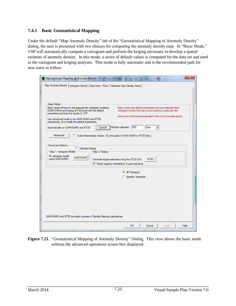
March 2014 Visual Sample Plan Version 7.0 7.23
7.4.1 Basic Geostatistical Mapping
Under the default “Map Anomaly Density” tab of the “Geostatistical Mapping of Anomaly Density”
dialog, the user is presented with two choices for computing the anomaly density map. In “Basic Mode,”
VSP will automatically compute a variogram and perform the kriging necessary to develop a spatial
estimate of anomaly density. In this mode, a series of default values is computed for the data set and used
in the variogram and kriging analyses. This mode is fully automatic and is the recommended path for
new users to follow.
Figure 7.21. “Geostatistical Mapping of Anomaly Density” Dialog. This view shows the basic mode
without the advanced operations screen box displayed.

Visual Sample Plan Version 7.0 March 2014 7.24
To use the automatic mode, click on the “Launch” button within the “Basic Mode” screen box
(Figure 7.21). Clicking on this button will launch a series of programs that will momentarily flash
several operational windows to the screen before returning to the “Geostatistical Mapping of Anomaly
Density” dialog. After successful completion of this process, the modeled variogram can be viewed by
clicking on the “Variogram Model” tab in the “Geostatistical Mapping of Anomaly Density” dialog.
Clicking on the “OK” button will close this dialog and load the anomaly density estimate map as an
overlay onto the main VSP site map. Clicking on the “Apply” button will load the results into VSP but
keep the geostatistical mapping window open. At this point, the primary VSP mapping tools can be used
to investigate the details of the estimated anomaly density map.
7.4.2 Advanced Mode Geostatistical Mapping
In the “Advanced” mode, the user is given complete control over all the parameter settings involved in the
variogram and kriging analysis. This mode is recommended for experienced users or when specific
analysis parameters are necessary.
Advanced mode is selected by clicking on the “Advanced” button under the “Map Anomaly Density” tab
of the “Geostatistical Mapping of Anomaly Density” dialog. Clicking on this button will open a screen
box with various selections for advanced mode operation (see Figure 7.22). One parameter setting is
directly available from this screen box. This is the averaging window diameter. This value specifies the
size of the averaging window for computing the anomaly density values used in the geostatistical
mapping. The variogram lag distance and kriging grid cell size also are affected by this parameter. The
lag distance is the separation distance between pairs of data points. The lag distance collects the data
pairs into groups based on separation distance and is discussed further below. The initial lag spacing and
kriging grid cell size are set to be one-sixth the averaging window diameter by default. If an averaging
window diameter other than the default value is desired, it should be changed before proceeding with the
next steps in the analysis. The initial lag spacing and kriging grid cell size also can be changed by
manually entering them using the advanced mode.
The first processing step in the “Advanced Mode” is to click on the button labeled “GAM/GAMV.” This
selection will initiate the variogram calculation and then open a separate screen presenting a graphical
interface for additional variogram analysis. At this point, the automatically fit variogram model can be
viewed by clicking on the “Fitting” tab of the GAM/GAMV” screen (see Figure 7.23). Here, the user
will see the empirical variogram values as well as the automatically fit variogram model and its
parameters (such as in Figure 7.24). The variogram is computed from the averaged anomaly density
values obtained from the geophysical survey transect data. The averaged anomaly densities are computed
automatically using the averaging window diameter specified under the “Advanced Options” screen box,
and the previously loaded anomaly locations and course over ground information. These values are then
passed automatically to the GAM/GAMV code.
The “Variogram Control Parameters” tab in the GAM/GAMV screen provides access to other variogram
analysis parameters. Details regarding these other input parameters are given in GAM/GAMV interface
code help files, and a full discussion can be found in Deutsch and Journel (1998). In general, the only
control parameters that might typically be altered at this stage in the analysis are the lag spacing, lag
tolerance, and number of lags to compute. These parameters control how the observations for computing
the empirical variogram are grouped and the maximum separation distance that should be considered.
These parameters are discussed further below.

March 2014 Visual Sample Plan Version 7.0 7.25
Figure 7.22. Advanced Mode for Geostatistical Anomaly Density Mapping

Visual Sample Plan Version 7.0 March 2014 7.26
Figure 7.23. Aspects of the GAM/GAMV Interface Screen
Figure 7.24. Variogram Fitting Screen from the GAM/GAMV Window. Dots show computed
variogram values, and the solid green line shows the model fitted to variogram values.
Parameters for this model are listed along the left side of the window.
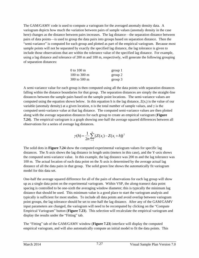
March 2014 Visual Sample Plan Version 7.0 7.27
The GAM/GAMV code is used to compute a variogram for the averaged anomaly density data. A
variogram depicts how much the variation between pairs of sample values (anomaly density in the case
here) changes as the distance between pairs increases. The lag distance—the separation distance between
pairs of data points—is used to group the data pairs into groups based on separation distance. Then the
“semi-variance” is computed for each group and plotted as part of the empirical variogram. Because most
sample points will not be separated by exactly the specified lag distance, the lag tolerance is given to
include those observations that are within the tolerance value of the specified lag distance. For example,
using a lag distance and tolerance of 200 m and 100 m, respectively, will generate the following grouping
of separation distances:
0 to 100 m group 1
100 to 300 m group 2
300 to 500 m group 3
A semi-variance value for each group is then computed using all the data points with separation distances
falling within the distance boundaries for that group. The separation distances are simply the straight-line
distances between the sample pairs based on the sample point locations. The semi-variance values are
computed using the equation shown below. In this equation h is the lag distance, Z(xi) is the value of our
variable (anomaly density) at a given location, n is the total number of sample values, and γ is the
computed semi-variance value at that lag distance. The computed semi-variance values are then plotted
along with the average separation distances for each group to create an empirical variogram (Figure
7.24). The empirical variogram is a graph showing one-half the average squared differences between all
observations for a series of average lag distances.
n
i
ii hxZxZn
h1
2))()((2
1)(
The solid dots in Figure 7.24 show the computed experimental variogram values for specific lag
distances. The X-axis shows the lag distance in length units (meters in this case), and the Y-axis shows
the computed semi-variance value. In this example, the lag distance was 200 m and the lag tolerance was
100 m. The actual location of each data point on the X-axis is determined by the average actual lag
distance of all the data pairs in that group. The solid green line shows the automatically fit variogram
model for this data set.
One-half the average squared difference for all of the pairs of observations for each lag group will show
up as a single data point on the experimental variogram. Within VSP, the along-transect data point
spacing is controlled to be one-sixth the averaging window diameter; this is typically the minimum lag
distance that should be used. This minimum value is a good place to start the variogram analysis and
typically is sufficient for most studies. To include all data points and avoid overlap between variogram
point groups, the lag tolerance should be set to one-half the lag distance. After any of the GAM/GAMV
input parameters are changed, the variogram will need to be recomputed by clicking on the “Compute
Empirical Variogram” button (Figure 7.23). This selection will recalculate the empirical variogram and
display the results under the “Fitting” tab.
The “Fitting” tab of the GAM/GAMV window (Figure 7.23) interface will display the computed
empirical variogram, and will also automatically compute an initial model to fit the data points. This

Visual Sample Plan Version 7.0 March 2014 7.28
model consists of a continuous function that closely matches the distribution of the empirical variogram
data points. A continuous function that will produce a positive definite covariance matrix for solving the
kriging equations is required as a model of spatial variability. Although a single model typically is
sufficient, up to three different models can be nested simultaneously to provide a proper fit to the
empirical data points. Excessive time should not be spent in creating a best-fit model of the empirical
variogram data. Typically, the focus of the variogram model fitting should be on matching the
experimental variogram points at the shorter lag spacings; the variance of the data set, shown by the solid
horizontal black line, provides the theoretical maximum variogram value (see Figure 7.25). A reasonably
good fit is usually sufficient when using sample transect data set.
The variogram model is reshaped by changing the range and sill values (Figure 7.25). The sill controls
the height of the variogram model while the range controls the distance scale of the model. If a large
initial jump in the variance is needed to match the empirical data, the nugget value can be increased. The
nugget, sill, and range can be adjusted to match the computed variogram data points as needed. In
addition, the basic model type (e.g., spherical, Gaussian, exponential) also can be changed as needed.
The variogram model line will change dynamically as any of the modeling parameters are altered.
Figure 7.25. Variogram model parameters settings within the GAM/GAMV Graphical Interface
Figure 7.26 shows the effects of changing the range and sill values of the variogram model. The sample
data for these plots were from a magnetometer survey of a portion of the Pueblo Precision Bombing
Range in southeastern Colorado. The magnetometer transects from this survey were nominally spaced at
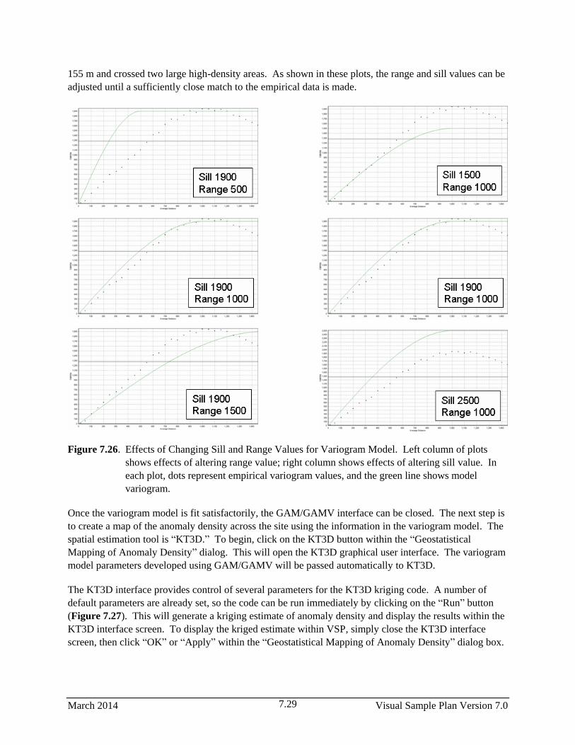
March 2014 Visual Sample Plan Version 7.0 7.29
155 m and crossed two large high-density areas. As shown in these plots, the range and sill values can be
adjusted until a sufficiently close match to the empirical data is made.
Figure 7.26. Effects of Changing Sill and Range Values for Variogram Model. Left column of plots
shows effects of altering range value; right column shows effects of altering sill value. In
each plot, dots represent empirical variogram values, and the green line shows model
variogram.
Once the variogram model is fit satisfactorily, the GAM/GAMV interface can be closed. The next step is
to create a map of the anomaly density across the site using the information in the variogram model. The
spatial estimation tool is “KT3D.” To begin, click on the KT3D button within the “Geostatistical
Mapping of Anomaly Density” dialog. This will open the KT3D graphical user interface. The variogram
model parameters developed using GAM/GAMV will be passed automatically to KT3D.
The KT3D interface provides control of several parameters for the KT3D kriging code. A number of
default parameters are already set, so the code can be run immediately by clicking on the “Run” button
(Figure 7.27). This will generate a kriging estimate of anomaly density and display the results within the
KT3D interface screen. To display the kriged estimate within VSP, simply close the KT3D interface
screen, then click “OK” or “Apply” within the “Geostatistical Mapping of Anomaly Density” dialog box.

Visual Sample Plan Version 7.0 March 2014 7.30
The other advanced options for running KT3D can be accessed through the various tabs under the main
“Parameters” tab on the interface screen. A complete explanation of these various options is presented in
the associated help files contained within the KT3D tool.
Figure 7.27. KT3D Interface Screen
The KT3D parameters most likely to be changed from their defaults are the gridding and search
parameters. These parameters, which control the number, size, and extent of the estimation cells used to
discretize the site and the search of local data to be used in the estimation of any location, respectively,
are located under the “Grid” and “Search/Discretization” tabs.
Typically, the default values for these parameters are sufficient and appropriate. These parameters are
explained fully in help files associated with the KT3D program, and a full discussion of the background
of the estimation can be found in Deutsch and Journel (1998). It is important to remember that the X and
Y node count and X and Y block sizes are used in conjunction to determine the area covered by the
kriging estimation; changing one without changing the other may result in a kriging estimation area which
is smaller or larger than your original transect sampling domain.
After all the parameters are set, the user clicks on the “Run” button to run KT3D. The kriging results are
displayed automatically within the KT3D interface sub-window. In addition to the anomaly density
estimate, the kriging variance is displayed in an adjacent window. Closing the KT3D interface window
will return the user to VSP and the “Map Anomaly Density” dialog. Clicking on “OK” or “Apply” will
display the kriging results in the VSP display.
7.4.3 Display of Kriging Results Within VSP
Whether run from “Basic” or “Advanced” mode, clicking on the “Apply” or “OK” button in the “Map
Anomaly Density” screen will display the current kriging results within the VSP mapping window. The
anomaly density map is displayed in VSP as a color-shaded value map. Figure 7.28 shows kriging
results displayed in VSP. The anomaly density estimate in Figure 7.28 was developed from

March 2014 Visual Sample Plan Version 7.0 7.31
magnetometer surveys from a portion of the Pueblo Precision Bombing Range. The site is a World War
II-era bombing range that shows evidence of two large target areas. The default color scheme in the map
display shows the highest density values in red and the lowest values in green. A color scale is provided
to aid in interpretation of the results. The lack of color shading (background color is displayed) indicates
that no kriging estimation was performed for that location. This typically is the result of a lack of enough
sample transect data within the search window for reliable estimates within that area. An example of this
Figure 7.28. Results of Kriging Estimation Displayed in VSP
can be seen in Figure 7.29 as a gray area in the northern portion of the study area. Transects were not
surveyed in this area because of vegetation and terrain issues. Because of this gap, no kriging estimates
were developed for this area.

Visual Sample Plan Version 7.0 March 2014 7.32
During examination of the anomaly density map, it is useful to turn on the display of the transect survey
traces and the detected anomaly locations as aids in interpreting the anomaly density map (Figure 7.29).
The controls for turning different map elements on and off are located under the “View” menu, or in the
“Layer Control” side bar of the main VSP screen. These provide a listing of different mapping elements
that can be checked on or off to control their display. The transect survey and detected anomaly locations
provide a visual relationship between the kriging results and the support data used in the kriging analysis.
For example, the transect traces shown in Figure 7.29 explain the gap in the kriging results in the
northern portion of the Pueblo Precision Bombing Range study area.
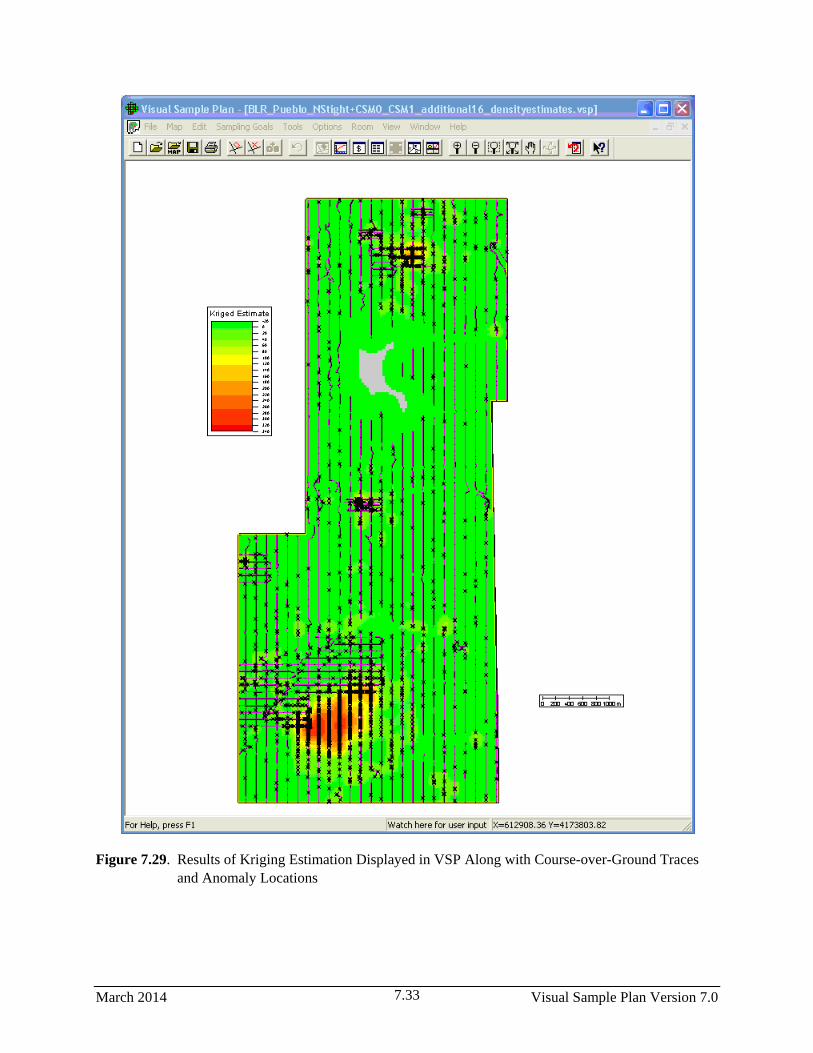
March 2014 Visual Sample Plan Version 7.0 7.33
Figure 7.29. Results of Kriging Estimation Displayed in VSP Along with Course-over-Ground Traces
and Anomaly Locations
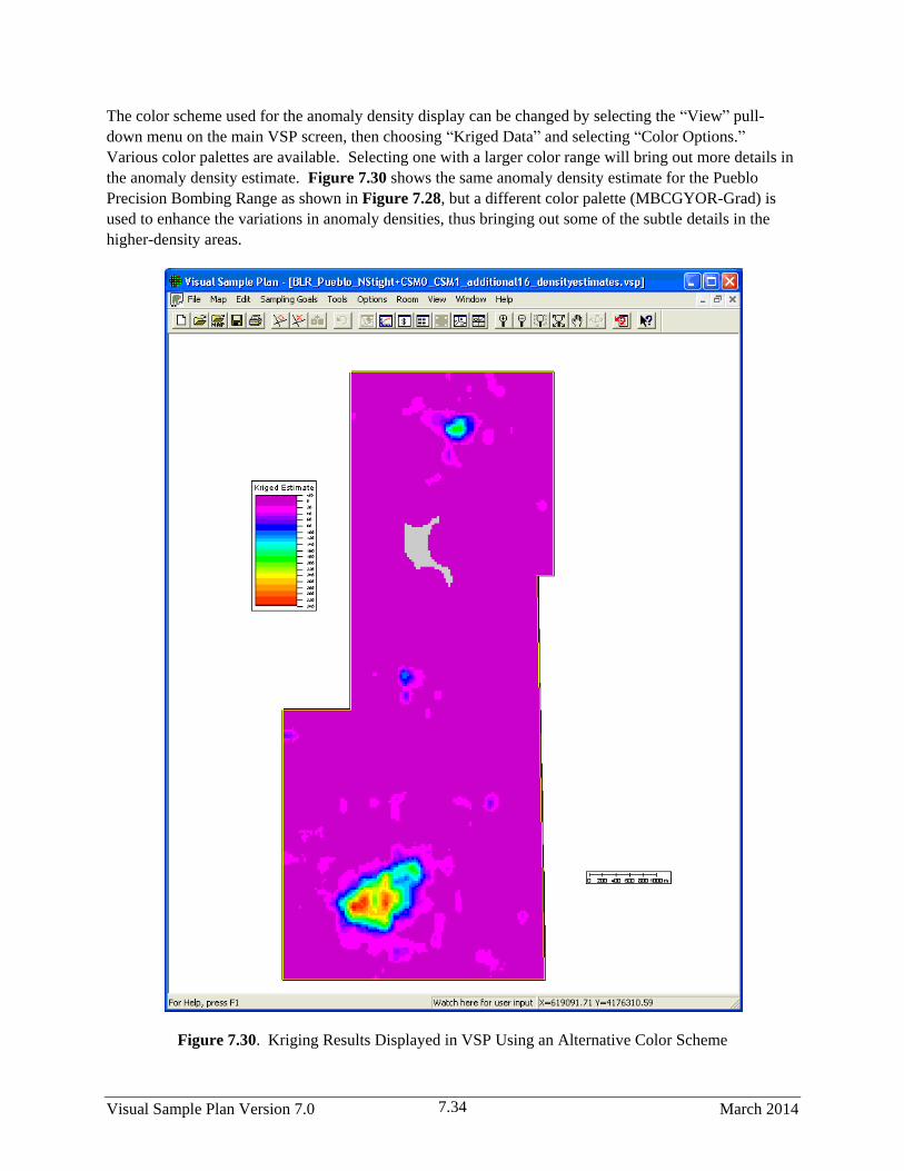
Visual Sample Plan Version 7.0 March 2014 7.34
The color scheme used for the anomaly density display can be changed by selecting the “View” pull-
down menu on the main VSP screen, then choosing “Kriged Data” and selecting “Color Options.”
Various color palettes are available. Selecting one with a larger color range will bring out more details in
the anomaly density estimate. Figure 7.30 shows the same anomaly density estimate for the Pueblo
Precision Bombing Range as shown in Figure 7.28, but a different color palette (MBCGYOR-Grad) is
used to enhance the variations in anomaly densities, thus bringing out some of the subtle details in the
higher-density areas.
Figure 7.30. Kriging Results Displayed in VSP Using an Alternative Color Scheme

March 2014 Visual Sample Plan Version 7.0 7.35
In addition to the estimate of anomaly density, the kriging procedure generates a map of the estimation
variance. Figure 7.31 shows the kriging estimation variance computed for the kriging results from the
Pueblo Precision Bombing Range study area. The estimation variance shows the uncertainty of the
kriging estimate and is a function of the data configuration and the variogram model. Estimates of
anomaly density for locations on or near sample transects should be very accurate and, hence, have a low
uncertainty. Conversely, estimates distant from the sample transects are likely to be less accurate with a
relatively high uncertainty. The value of the estimation variance reaches a maximum at distances greater
than or equal to the variogram range away from the nearest data point. The map of estimation variance
shows how the variance of the anomaly density changes across the study site. In Figure 7.31, the highest
variance values are shown in shades of red; the lowest values in shades of green. The highest variance
values occur in the northern portion of the site where there is a large gap in the sample transects because
of terrain and vegetation issues. The maximum variances occur on the edge of the region where no
estimates could be made. These high variance values indicate that some areas exist within the site where
there are enough nearby data points to create a kriging estimate, but the uncertainty in these estimates is
large. While not explored further here, the kriging variance provides a means of identifying regions of
high uncertainty and can be used to design additional transect surveys. The lowest variance values are
found at the survey transect locations.
The anomaly density estimates can be exported to a file format that is compatible with the ESRI ArcGIS
geographic information software system. This is done by selecting “Map > Export” from the main VSP
screen. This will provide options for exporting the current kriging estimates or the kriging variances.
Maintaining the filename extension of “ASC” will provide direct recognition of the export file within
ArcGIS. This export file format can be read directly into ArcGIS.
To view the estimation variance, select the “View” pull-down menu on the main VSP screen, then choose
“Kriged Data” and select “Kriging Variance.” As shown in Figure 7.31, there is a strong relationship
between the sample transect locations and the kriging variance. The variance is lowest near the transects
and increases with increasing distance from the sample locations. This can be used as a quick check to
confirm that all the appropriate sample data have been included in the kriging analysis and to identify
areas where the confidence in the kriging results could be increased with additional sample data.

Visual Sample Plan Version 7.0 March 2014 7.36
Figure 7.31. Kriging Variance Displayed in VSP Along with Course-over-Ground Traces. The highest
variance values are shown in red, the lowest values in green.

March 2014 Visual Sample Plan Version 7.0 7.37
7.5 Delineating High-Density Areas
Tools for delineating high anomaly density areas can be found under the “Delineate High Density Areas”
tab of both the flagging menu window and the geostatistical mapping menu window. These can be
accessed by selecting Sampling Goals > Find Target Areas and Analyze Survey Results (UXO) >
Locate and mark target areas based on elevated anomaly density or, Sampling Goals > Find Target
Areas and Analyze Survey Results (UXO) > Geostatistical Mapping of Anomaly Density from the
VSP menu. Figure 7.32 shows the high density area delineation window when accessed from the
“Locate and mark target areas…” window. This window contains selection buttons for activating the
delineation tools and a table listing the results of the delineation process.
Figure 7.32. Delineation window.

Visual Sample Plan Version 7.0 March 2014 7.38
7.5.1 Delineation from Target Flagging Results
To use the delineation tool based on transect flagging results, the flagging must be performed prior to
using the delineation tool. When the “Automatic from Target Markers” button is selected, the window
shown in Figure 7.33 is displayed. This window lists the parameters for delineation using the results
from target area flagging.
Figure 7.33. Target area delineation parameters
The parameters for high anomaly density (target) area delineation based on flagging results consist of the
block size to put around each marker flag and the minimum size of a high density area to be considered
for delineation. The block size parameter specifies the XY extent of the area around each flagged high
density location to be included in the designation of a target area. It is important that this value be
slightly larger than the transect sample spacing in order for adjacent transects to be grouped together into
a common target area. If this value is too small, then adjacent transects with high density locations will
be marked as individual target locations instead of being grouped together.
The Minimum size of target area specifies a size threshold below which a delineated area is considered
too small to be a valid target feature. All delineated areas below this threshold are dropped from the
listing of delineated areas and not added to the table of potential target areas. Be sure to choose
appropriated units for this value. For reference, the parameters window provides the diameter of a circle
of the minimum target area size.
Once the appropriate values for all the parameters are set the “OK” button can be clicked. This will run
the target area delineation and present the results in a table as shown in Figure 7.34. The table in the
upper portion of this window lists all the high density areas delineated for the active sample areas. Each
entry is color coded with a color, which correlates to the colored regions shown on the map view (Figure
7.35).
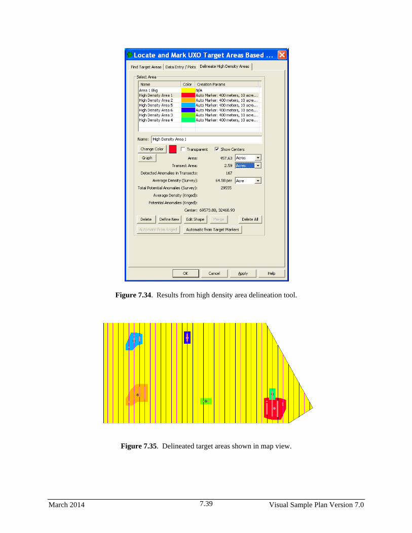
March 2014 Visual Sample Plan Version 7.0 7.39
Figure 7.34. Results from high density area delineation tool.
Figure 7.35. Delineated target areas shown in map view.

Visual Sample Plan Version 7.0 March 2014 7.40
When each delineated target area row in the table is selected, the spatial statistics for that delineated area
are displayed in the window. These include the total area, total transect length falling within, total
number of anomalies, etc. for that delineated area.
The “Change Color” button allows you to customize the color used for each delineated area. The
“Graph” button will plot a histogram or box-and-whiskers plot for the selected delineated area. The
“Name” text box allows you to change the text name associated with each delineated area. The
“Transparent” check box replaces the color fill for the delineated areas with a colored polygon outline and
the “Show Centers” check box places a circle with cross-hairs symbol at the center of each delineated
area.
In addition, the lower portion of the window displays buttons to delete individual areas, manually define
new areas by drawing a polygon, edit the shape of an existing area, or merge two adjacent areas. Any
modifications to a delineated area will be recorded for that area and displayed in the table listing. The
“Delete All” button will delete all the delineated areas. This is very useful when investigating different
delineation threshold values in an iterative fashion.
7.5.2 Delineation from Geostatistical Estimation of Anomaly Density Results
The process for delineating high density areas based on the results of geostatistical estimation is very
similar to that used for the flagging results. The geostatistical estimation of anomaly density must be
completed prior to using the delineation tool.
For delineating areas based on the results from geostatistical estimation, the delineation window is
accessed as described above and can be found either from the flagging window or the geostatistical
estimation window. If a kriged estimate of anomaly density is available, then the “Automatic from
Kriged” button will be active. Clicking on this button will bring up the “Parameters for Target
Delineation” window as shown in Figure 7.36. There are two parameters which may be set from this
window. The minimum target area size parameter controls the smallest region considered as a valid
target area. This is the same parameter as was described under the delineation from flagging results
procedure. The minimum kriged value specifies the threshold for delineating a target area. Regions with
anomaly densities at or above this threshold will be delineated as a potential target area if they meet the
minimum size criteria. Once the parameters are set, clicking on the “OK” button will run the delineation
process and display the results in a window similar to that shown in Figure 7.34.
All the other options for investigating and interacting with the delineated target areas described under the
flagging delineation also apply to the results from the geostatistical estimation delineation.

March 2014 Visual Sample Plan Version 7.0 7.41
Figure 7.36. Parameters for target area delineation using geostatistical anomaly density estimates.
7.5.3 Plotting Results from Delineation
Comparative plots of the anomaly density values for the different delineated areas can be viewed by
clicking on the “Data Entry/Plots” tab, then selecting the “Plots” sub-tab (Figure 7.37). This sub-tab
provides access to color-coded histograms and box-and-whisker plots comparing the anomaly density
values of the various delineated areas and background (shown in the color of the sample area). An
example box-and-whisker plot displaying the results from an example target area delineation are shown in
Figure 7.37. These plots are extremely valuable in making target area to background comparisons and in
investigating the anomaly density distribution of individual delineated areas. The type of plot displayed
(histogram or box-and-whisker) is set by the pull-down control in the upper-right corner of the window.
There are several other options in the “Plots” sub-tab which are activated by buttons near the bottom of
the window. These options are summarized in Table 7.3 below.
Table 7.3. Plotting options.
Option Control Action
Log Y check box Use log based Y-axis in histogram
Max Y value Set maximum Y-axis value in histogram
Bins value Number of bins to use for histogram
Color check box Use colors to code source for histogram values
Bk. v. All check box Compare background to all delineated areas combined
Order button Change the plotting order of the different elements
Show Outliers button Plot a symbol on map indicating location of outliers
Pick Map Area button Only plot data falling within a user defined rectangle on map
Reset button Reset all plotting options to default values
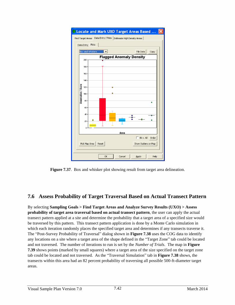
Visual Sample Plan Version 7.0 March 2014 7.42
Figure 7.37. Box and whisker plot showing result from target area delineation.
7.6 Assess Probability of Target Traversal Based on Actual Transect Pattern
By selecting Sampling Goals > Find Target Areas and Analyze Survey Results (UXO) > Assess
probability of target area traversal based on actual transect pattern, the user can apply the actual
transect pattern applied at a site and determine the probability that a target area of a specified size would
be traversed by this pattern. This transect pattern application is done by a Monte Carlo simulation in
which each iteration randomly places the specified target area and determines if any transects traverse it.
The “Post-Survey Probability of Traversal” dialog shown in Figure 7.38 uses the COG data to identify
any locations on a site where a target area of the shape defined in the “Target Zone” tab could be located
and not traversed. The number of iterations to run is set by the Number of Trials. The map in Figure
7.39 shows points (marked by small squares) where a target area of the size specified on the target zone
tab could be located and not traversed. As the “Traversal Simulation” tab in Figure 7.38 shows, the
transects within this area had an 82 percent probability of traversing all possible 500-ft-diameter target
areas.
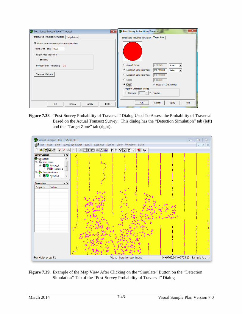
March 2014 Visual Sample Plan Version 7.0 7.43
Figure 7.38. “Post-Survey Probability of Traversal” Dialog Used To Assess the Probability of Traversal
Based on the Actual Transect Survey. This dialog has the “Detection Simulation” tab (left)
and the “Target Zone” tab (right).
Figure 7.39. Example of the Map View After Clicking on the “Simulate” Button on the “Detection
Simulation” Tab of the “Post-Survey Probability of Traversal” Dialog

Visual Sample Plan Version 7.0 March 2014 7.44
7.7 Analyze 100% Survey of Sample Areas
In some cases, it is possible to conduct a Geophysical survey that covers an entire DoD site or facility to
map the density of anomalous metallic readings in order to search for Target Areas at which munitions
were fired or dropped. This is opposed to the usual case where only a small portion of the site is surveyed
by geophysical detectors at widely spaced linear intervals, referred to as transects.
The mapping of anomaly densities provides a continuous estimate of the density of metallic anomalies for
the entire study site. This spatially continuous representation is important for the detection of high density
areas and for providing a basis for other spatial analyses. The basic output from this process is a map
showing an estimate of how the metallic anomaly density varies across the study site. The only input to
the process (other than the site map) is a list of all anomaly location coordinates. The anomaly locations
can be imported on the data page. This is reached by opening the module and going to the Data Entry
sub-page by selecting Sampling Goals > Find Target Areas and Analyze Survey Results (UXO) >
Analyze 100% survey sample areas and clicking on the “Data Entry” tab. Clicking “Import” allows one
or more anomaly files to be imported as shown in Figure 7.40.
Figure 7.40. Data Entry for Anomaly Data
After anomaly locations are imported into VSP, there are two parameters that are needed to create the
density map: grid size and smoothing level. Grid size can be done automatically using the defaults, or it
can be changed by the user. The site is subdivided into grid cells and the density of each is computed.
The smoothing level is used to minimize drastic density differences between adjacent grid cells. The
smoothing level can be set to minimum, medium or maximum. The default smoothing level is medium,
until changed by the user.
Clicking on the Apply button will initiate the process of dividing each sample area into grid cells,
computing the density for each grid cell, smoothing the density values and displaying the density map.
The anomaly density map is displayed in VSP as a color-shaded value map such as in Figure 7.41. High
density areas can be delineated in a similar manner to previously discussed modules by going to the
Delineate High Density Areas tab.

March 2014 Visual Sample Plan Version 7.0 7.45
Figure 7.41. Anomaly Density Map
7.8 Post Remediation Verification Sampling
The UXO modules in VSP for Post Remediation Verification Sampling (UXO) assist in developing a
sampling strategy to achieve high confidence that very few targets of interest (TOI) are present at a site or that
very few detected anomalies at a site are TOI. The two modules can be used to determine the number of
transects that should be surveyed to establish Y% confidence that at least X% of the transects at the site do not
contain TOI, where Y, X, and the number of transects are entered by the user. The same method can be
applied to detected anomalies to determine the number of detected anomalies to dig up to establish Y%
confidence that at least X% of the detected anomaly locations do not contain TOI.
In the Sampling Goal covered in this section, if there are TOI, they are limited and isolated objects not in
any particular pattern. Two scenarios of interest are 1) a small UXO-remediated area where a survey is
required to support a no-further-action (NFA) decision and 2) a very large unremediated area not
expected to contain any TOI. In both scenarios, we assume the area of interest has a well-defined
boundary. The area is divided into N non-overlapping, parallel transects with transect width equal to the
width of the geophysical survey equipment. If N is large and only n of these transects can be surveyed,
how should n be determined? This is similar to a compliance sampling problem in an industrial quality
control setting where the goal is to determine if there are any defects before releasing a product.

Visual Sample Plan Version 7.0 March 2014 7.46
VSP addresses the variant of the problem where n must be of sufficient size to achieve a high confidence
that few transects contain TOI. The method can also be applied to anomalies detected during a survey to
achieve a high confidence that few detected anomalies are TOI.
7.8.1 Achieve High Confidence That Few Transects Contain UXO
Menu selection Sampling Goals > Post Remediation Verification Sampling (UXO) > Transect
verification sampling brings up the dialog box in Figure 7.42 where the Transect Verification Sampling
(left) and Transect Placement (right) tabs are shown. We enter a transect width of 2 m and a grid
dimension (grid dimension and orientation is assumed to be aligned with the remediation grids) of 100 x
100 m. VSP informs us that there are N = 62,050 total nonoverlapping transects within this Sample Area.
The VSP user enters 99% as the minimum number of transects required to not contain one or more UXO
(DQO input) and 95% as the confidence that this maximum percentage is not exceeded. VSP calculates
that 298 of the 62,050 transects must be selected, using random sampling, and none of these transects can
contain TOI in order to be “95% confident that at least 99% of the possible transects at the site do not
contain TOI. The n =298 selected transects are randomly selected in length aggregated groups of 3
transects at 100 randomly selected locations. Attribute Compliance Sampling (ACS) (Schilling 1978;
1983, pages 475-482) is a statistical approach for establishing confidence in the cleanup effort. The
sample size equation programmed into VSP for this problem is a method from Bowen and Bennett
(1988). For extensive discussion of this problem and compliance sampling methods, consult VSP Help,
Gilbert et al. (2003, Chapter 6) or Hathaway et al. (2008).
Figure 7.42. Dialog Input Box for Verification Sampling of TOI for the Transect Verification Sampling
(left) and Transect Placement (right) tabs.

March 2014 Visual Sample Plan Version 7.0 7.47
7.8.2 Achieve High Confidence That Few Anomalies are UXO
Menu selection Sampling Goals > Post Remediation Verification Sampling (UXO) > Anomaly
verification sampling brings up the dialog box in Figure 7.43. Using the Millsite.dxf map and the large
elliptical area selected as our Sample Area, we now include some data on anomaly locations. The 137
anomalies are shown either as small black “x” or small pink circles in Figure 7.37. The VSP user enters
90% as the minimum percent of anomalies required to not be TOI and 90% as the confidence that this
maximum percentage is not exceeded.
VSP calculates that 39 of the 137 anomalies must be selected, using simple random sampling, and none of
these anomalies can be UXO in order to be “90% confident that at least 90% of the possible anomalies at
the site are not TOI. The n = 39 randomly selected anomalies are shown on the map as small pink circles
when the Apply button is pushed, as shown in Figure 7.43. The sample size equation programmed into
VSP for this problem is a method from Bowen and Bennett (1988).
Figure 7.43. Dialog Input Box for Anomaly Sampling for UXO and Map of Sample Area with
Anomalies Selected
7.9 Remedial Investigation
Selecting Sampling Goals > Remedial Investigation provides access to four different designs related to
investigating a site with suspected unexploded ordnance (UXO):
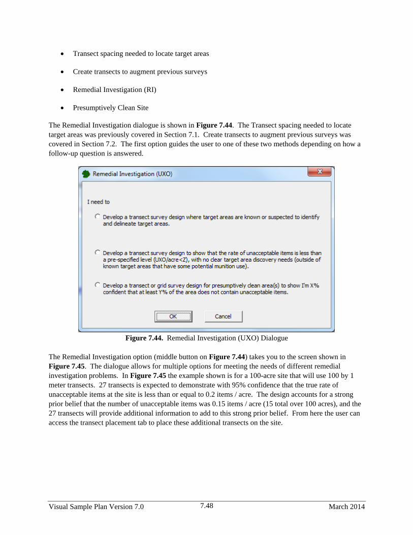
Visual Sample Plan Version 7.0 March 2014 7.48
Transect spacing needed to locate target areas
Create transects to augment previous surveys
Remedial Investigation (RI)
Presumptively Clean Site
The Remedial Investigation dialogue is shown in Figure 7.44. The Transect spacing needed to locate
target areas was previously covered in Section 7.1. Create transects to augment previous surveys was
covered in Section 7.2. The first option guides the user to one of these two methods depending on how a
follow-up question is answered.
Figure 7.44. Remedial Investigation (UXO) Dialogue
The Remedial Investigation option (middle button on Figure 7.44) takes you to the screen shown in
Figure 7.45. The dialogue allows for multiple options for meeting the needs of different remedial
investigation problems. In Figure 7.45 the example shown is for a 100-acre site that will use 100 by 1
meter transects. 27 transects is expected to demonstrate with 95% confidence that the true rate of
unacceptable items at the site is less than or equal to 0.2 items / acre. The design accounts for a strong
prior belief that the number of unacceptable items was 0.15 items / acre (15 total over 100 acres), and the
27 transects will provide additional information to add to this strong prior belief. From here the user can
access the transect placement tab to place these additional transects on the site.

March 2014 Visual Sample Plan Version 7.0 7.49
Figure 7.45. Remedial Investigation Target of Interest (TOI) Estimation / Comparison
The presumptively clean site option (bottom button on Figure 7.44) takes you to the screen shown in
Figure 7.46. The dialogue allows for multiple options for meeting the needs of different remedial
investigation problems. In Figure 7.46 the example shown is for a 100-acre site that will use 100 by 1
meter transects. 67 transects is expected to demonstrate with 95% confidence that 98% or more of the
parcels at the site are acceptable. The design accounts for a strong prior belief that the number of
unacceptable is 50 or less, and the 67 transects will provide additional information to add to this prior
belief. From here the user can access the transect placement tab to place these additional transects on the
site.
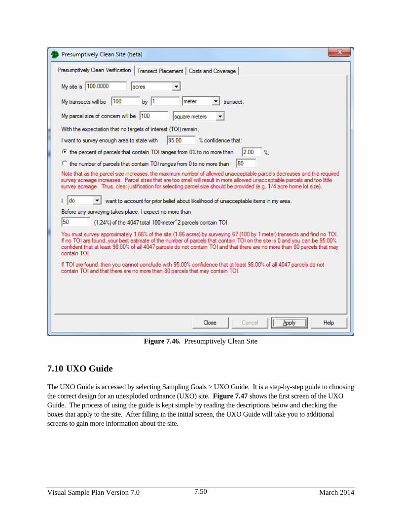
Visual Sample Plan Version 7.0 March 2014 7.50
Figure 7.46. Presumptively Clean Site
7.10 UXO Guide
The UXO Guide is accessed by selecting Sampling Goals > UXO Guide. It is a step-by-step guide to choosing
the correct design for an unexploded ordnance (UXO) site. Figure 7.47 shows the first screen of the UXO
Guide. The process of using the guide is kept simple by reading the descriptions below and checking the
boxes that apply to the site. After filling in the initial screen, the UXO Guide will take you to additional
screens to gain more information about the site.

March 2014 Visual Sample Plan Version 7.0 7.51
Figure 7.47. UXO Guide

March 2014 Visual Sample Plan Version 7.0 8.1
8.0 References
Agresti, A., & Coull, B. (1998). Approximate is better than "exact" for interval estimation of binomial
proportions. The American Statistician, 52(2), 119-126.
Bowen, M.W. and C.A. Bennett. 1988. Statistical Methods for Nuclear Material Management,
NUREG/CR-4604, U.S. Nuclear Regulatory Commission, Washington, DC
B. W. Brown, Jr., M. Hollander, and R. M. Korwar, Nonparametric tests of independence for censored
data, with applications to heart transplant studies, Reliability and Biometry: Statistical Analysis of
Lifelength, F. Proschan and R. J. Serfling, (eds.), pp. 327-354, SIAM: Philadelphia, 1974.
Brown, G. H. and N. I. Fisher. 1972. Subsampling a Mixture of Sampled Material. Technometrics 14(3):
663-&.
Cameron, K. 2004, "Better Optimization of Long-Term Monitoring Networks." Bioremediation Journal
8:89-107.
Cameron, K, and P Hunter. 2002, "Using Spatial Models and Kriging Techniques to Optimize Long-Term
Ground-Water Monitoring Networks: A Case Study." Environmetrics 13:629-59.
Chernick, M. R., and Liu, C. Y. (2002). The saw-toothed behavior of power versus sample size and
software solutions: Single binomial proportion using exact methods. The American Statistician, 56, 149-
155.
Cleveland W.S. 1979. “Robust Locally Weighted Regression and Smoothing Scatterplots.” Journal of the
American Statistical Association, Vol. 74, No. 368. p. 829-836.
Cochran, W.G. 1977. Sampling Techniques, 3rd edition. John Wiley & Sons, New York.
Conover,WJ. 1980. Practical Nonparametric Statistics. John Wiley and Sons, New York.
Davidson, J. R. 1995. ELIPGRID-PC: Upgraded Version. ORNL/TM-13103, Oak Ridge National
Laboratory, Oak Ridge, Tennessee.
Devore, J. L., 1991, Probability and Statistics for Engineering and the Sciences, Belmont, CA,
Wadsworth, Inc.
Duetsch CV and AG Journel. 1998. GSLIB Geostatistical Software Library and User’s Guide. 2nd
Edition, Applied Geostatistics Series, Oxford University Press, Inc. New York.
Elder, R. S., W. O. Thompson, et al. 1980. Properties of Composite Sampling Procedures. Technometrics
22(2): 179-186.
Esterby, S.R. Review of methods for the detection and estimation of trends with emphasis on water
quality applications , Hydrological Processes 10:127-149.
Fisher, R. A., 1970, Statistical Methods for Research Workers, New York, NY, Hafner Press.

Visual Sample Plan Version 7.0 March 2014 8.2
Geosoft Inc., 2007, Oasis Montaj Users Manual Version 6.4, available at www.geosoft.com, 290 p.
Gibbons, J.D., and S. Chakraborti. 2003. Nonparametric Statistical Inference, Marcel Dekker, NY.
Gilbert, R.O., J. E. Wilson, B. A. Pulsipher, N. L. Hassig, and L. L. Nuffer. 2005. Technical
Documentation and Verification for the Buildings Module in the Visual Sample Plan (VSP) Software.
PNNL-15202. Pacific Northwest National Laboratory, Richland, Washington.
Gilbert, R.O., J. E. Wilson, B. A. Pulsipher. 2005. Visual Sample Plan User’s Guide for Establishing the
Boundary of Contamination. PNWD-3580. Battelle-Pacific Northwest Division, Richland, Washington.
Gilbert, R., J. Wilson, et al. 2005. Technical Documentation and Verification for the Buildings Module in
the Visual Sample Plan (VSP) Software. Pacific Northwest National Laboratory, Richland, Washington.
Gilbert, R. O, J. E. Wilson, R. F. O’Brien, D. K. Carlson, D. J. Bates, B. A. Pulsipher, and
C. A. McKinstry. 2002. Version 2.0 Visual Sample Plan (VSP) Models and Code Verification.
PNNL-13991, Pacific Northwest National Laboratory, Richland, Washington.
Gilbert, R. O, J. E. Wilson, R. F. O’Brien, D. K. Carlson, B. A. Pulsipher, and D. J. Bates. 2003.
Version 2.0 Visual Sample Plan (VSP): UXO Module Code Description and Verification.. PNNL-14267,
Pacific Northwest National Laboratory, Richland, Washington.
Gilbert, R. O. 2003. Results of QA Testing of the Visual Sample Plan (VSP) Collaborative Sampling
(CS) Module PNNL Milestone Report to EPA Quality Staff, Pacific Northwest National Laboratory,
Richland, Washington.
Gilbert, RO, JR Davidson, JE Wilson, BA Pulsipher. 2001. Visual Sample Plan (VSP) models and code
verification. PNNL-13450, Pacific Northwest National Laboratory, Richland, Washington.
Gilbert, R.O., B.A. Pulsipher, D.K. Carlson, R.F. O’ Brien, J.E. Wilson, D.J. Bates and G.A. Sandness.
2001. Designing UXO Sensor Surveys for Decision Making, Pacific Northwest National Laboratory,
Richland, WA.
Gilbert, R. O. 1987. Statistical Methods for Environmental Pollution Monitoring. John Wiley & Sons,
Inc., New York.
Goovaerts, P. 1997. Geostatistics for Natural Resources Evaluation. Applied Geostatistics Series, Oxford
University Press, New York.
Guenther, W. C. 1982. Normal Theory Sample-Size Formulas for Some Non-Normal Distributions.
Communications in Statistics Part B-Simulation and Computation 11(6): 727-732.
Gurland, John and Tripathi, Ram C. 1971. A Simple Approximation for Unbiased Estimation of the
Standard Deviation. The American Statistician. 25:30-32.
Hahn, GJ. and WQ Meeker. 1991. Statistical intervals a guide for practitioners. John Wiley & Sons, New
York.

March 2014 Visual Sample Plan Version 7.0 8.3
Hathaway, J, B. A. Pulsipher, J. E. Wilson, C. A. McKinstry. 2006. Final Report for Statistical Methods
and Tools for UXO Site Characterization on Final Simulated Site. PNNL- 15651, Pacific Northwest
National Laboratory, Richland, Washington.
Hathaway, J.E., B. Roberts, S. McKenna, B.A. Pulsipher. 2007. Using the VSP-UXO Modules to
Support Site Characterization. PNNL-17382. Pacific Northwest National Laboratory, Richland,
Washington.
Hathaway JE, GB Schaalje, RO Gilbert, BA Pulsipher, and BD Matzke. 2008. "Determining the
Optimum Number of Increments in Composite Sampling." Environmental and Ecological Statistics
15(3):313-327.
Hathaway J, RO Gilbert, JE Wilson, and BA Pulsipher. 2008. "Compliance Sampling Applications in
MEC Clean-Up at Military Training Sites." Stochastic Environmental Research and Risk Assessment.
Helsel, D.R. 2005. Nondetects and Data Analysis, Statistics for Censored Environmental Data, Wiley &
Sons, New York, NY.
Helsel, D.R. and R.M. Hirsch. 1995. Statistical Methods in Water Resources. Elsevier, NY.
Hirsch, R.M., J.R. Slack, and R.A. Smith. 1982. Techniques of trend analysis for monthly water quality
data, Water Resources Research 18(1):107-121.
Hirsch, R.M. and J.R. Slack. 1984. A nonparametric trend test for seasonal data with serial dependence.
Water Resources Research 20(6):727-732.
Isaaks, EH, and RM Srivastava. 1989. An Introduction to Applied Geostatistics. Oxford University Press,
New York.
Jaech, J.L. 1973. Statistical Methods in Nuclear Material Control, TID-26298, NTIS, Springfield,
Virginia.
Kendall, M.G. 1975. Rank Correlation Methods, 4th edition, Charles Griffin, London.
Kyriakidis, PC. 1997. Selecting Panels for Remediation in Contaminated Soils Via Stochastic Imaging. In
Geostatistics Wollongong '96 , eds. EY Baafi and NA Schofield, Vol 2, pp. 973-83. Kluwer Academic
Publishers, Dordrecht.
Lyles, R.H. and L.L. Kupper. 1996. On Strategies for Comparing Occupational Exposure Data to Limits,
American Industrial Hygiene Association Journal 57:6-15.
Mann, H.B. 1945. Non-parametric tests against trend, Econometrica 13:163-171.
Matzke BD, JE Wilson, and BA Pulsipher. 2006. Version 4.4 Visual Sample Plan (VSP): New UXO
Module Target Detection Methods. PNNL-15843, Pacific Northwest National Laboratory, Richland,
WA.
Visual Sample Plan Version 7.0 March 2014 8.4
Matzke BD, JE Wilson, and DA Damstedt. 2008. Visual Sample Plan (VSP): QA of UXO Module
Target Detection Methods . PNNL-17286, Pacific Northwest National Laboratory, Richland, WA.
Matzke BD, JE Wilson, J Hathaway, and BA Pulsipher. 2006. "Methods for Determining Probabilities
of Detection for Target Areas at DoD Munitions Sites." PNNL-SA-53289, Pacific Northwest National
Laboratory, Richland, WA.
Matzke BD, JE Wilson, and BA Pulsipher. 2006. Version 4.4 Visual Sample Plan (VSP): New UXO
Module Target Detection Methods. PNNL-15843, Pacific Northwest National Laboratory, Richland, WA.
Matzke BD, JE Wilson, J Hathaway, and BA Pulsipher. 2008. "Statistical Algorithms Accounting for
Background Density in the Detection of UXO Target Areas at DoD Munitions Sites." Stochastic
Environmental Research and Risk Assessment 23(2(2009)):181.
Matzke BD, JE Hathaway, LH Sego, BA Pulsipher, SA McKenna, JE Wilson, ST Dowson, LL Nuffer,
RO Gilbert, BL Roberts, NL Hassig, CJ Murray. 2010. Visual Sample Plan Version 6.0 User’s Guide .
PNNL-19915, Pacific Northwest National Laboratory, Richland, WA.
McIntyre, G.A. 1952. A method for unbiased selective sampling using ranked sets, Australian Journal of
Agricultural Research 3:385-390.
Millard, S.P. and N.K. Neerchal. 2001. Environmental Statistics with S-Plus. CRC Press, New York, NY.
Miller, R.G. 1986. Beyond ANOVA: The Basics of Applied Statistics, New York, Wiley.
Montgomery, Douglas C. 2001. Introduction to Statistical Quality Control, 4th ed. John Wiley & Sons,
Inc.
Owen, D. B. 1962. Handbook of statistical tables. Reading, Mass., Addison-Wesley.
Patil, G.P., A.K. Sinha and C. Taillie. 1994. Ranked set sampling, Handbook of Statistics 12,
Environmental Statistics, pp. 167-200, (G.P. Patil and C.R. Rao, editors), North-Holland, New York, NY.
Perez, A., and J.J. Lefante. 1997. Sample size determination and the effect of censoring when estimating
the arithmetic mean of a lognormal distribution. Communications in Statistics, Theory and Methods 26
(11):2779-2801.
Press, W. H., S. A. Teukolsky, W. T. Vetterling, and B. P. Flannery. 1993. Numerical Recipes in C: The
Art of Scientific Computing. 2nd ed. Cambridge University Press, United Kingdom.
Ramsey, F. L., and Schafer, D. W., 2002, The Statistical Sleuth: A Course in Methods of Data Analysis,
Belmont, CA: Duxbury Press.
Rohlf, F. J., H. R. Akcakaya, et al. 1996. Optimizing composite sampling protocols. Environmental
Science & Technology 30(10): 2899-2905.
Schilling, E.G. 1982. Acceptance Sampling in Quality Control, Marcel Dekker, Inc, New York.

March 2014 Visual Sample Plan Version 7.0 8.5
Sego, L.H. and J.E. Wilson. 2007. Accounting for False Negatives in Hot Spot Detection.
PNNL-16812. Pacific Northwest National Laboratory, Richland, WA, August 2007.
http://www.pnl.gov/main/publications/external/technical_reports/PNNL-16812.pdf
Singer, D.A. and J.E. Wickman. 1969. Probability Tables for Locating Elliptical Targets with Square,
Rectangular, and Hexagonal Point Nets. Pennsylvania State University, University Park, Pennsylvania.
Special Publication 1-69.
Singer, D.A. 1972. ELIPGRID: A Fortran IV program for calculating the probability of success in
locating elliptical targets with square, rectangular and hexagonal grids. Geocom Programs 4:1-16.
Squeglia, N.L. 1994. Zero Acceptance Number Sampling Plans. ASQ Quality Press, Milwaukee, WI.
Thompson, S. K. 1990. Adaptive Cluster Sampling. Journal of the American Statistical
Association 85:412.
Thompson, S.K. and G.A.F. Seber. 1996. Adaptive Sampling. John Wiley & Sons, New York.
Tuckfield, RC. 1994, "Estimating an Appropriate Sampling Frequency for Monitoring Ground Water
Well Contamination." Presented at International Nuclear Materials Management (INMM) Annual
Meeting: Naples. Available through DOE Office of Scientific and Technical Information,
http://www.osti.gov/bridge//product.biblio.jsp?query_id=1&page=0&osti_id=10177871
Webster, R, and MA Oliver. 1993, "How Large a Sample Is Needed to Estimate the Regional Variogram
Adequately?" in Geostatistics Troia '92, ed. A Soares, Vol 1, pp. 155-66. Kluwer Academic Publishers,
Dordrecht.
Wilson JE. 2013. Methodology for Defining Gap Areas between Course-over-ground Locations.
PNNL-22851, Pacific Northwest National Laboratory, Richland, WA.
http://www.pnl.gov/main/publications/external/technical_reports/PNNL-22851.pdf
Wilson JE. 2013. Methodology for Augmenting Existing Paths with Additional Parallel
Transects. PNNL-22770, Pacific Northwest National Laboratory, Richland, WA.
http://www.pnl.gov/main/publications/external/technical_reports/PNNL-22770.pdf
EPA. 1997. Multi-Agency Radiation Survey and Site Investigation Manual (MARSSIM).
EPA 402-R-97-016, NUREG-1575, U.S. Environmental Protection Agency, Washington, D.C.
EPA. 2000a. Guidance for the Data Quality Objectives Process - QA/G-4. EPA/600/R-96/055, Office of
Environmental Information, U.S. Environmental Protection Agency, Washington, D.C.
EPA. 2000b. Guidance for Data Quality Assessment - Practical Methods for Data Analysis - QA/G-9,
QA00 Update. EPA/600/R/96/084, Office of Environmental Information, U.S. Environmental Protection
Agency, Washington, D.C.

Visual Sample Plan Version 7.0 March 2014 8.6
EPA, November 2001. Guidance for Choosing a Sampling Design for Environmental Data Collection,
EPA QA/G-5S, Peer Review Draft, Washington, D.C.
EPA. 2002. Guidance for Choosing a Sampling Design for Environmental Data Collection, QA/G-5S,
Peer Review Draft. Office of Environmental Information, U.S. Environmental Protection Agency,
Washington, D.C.
EPA. 2006a. Guidance on Systematic Planning Using the Data Quality Objectives Process. EPA
QA/G-4, EPA/240/B-06/001, U.S. Environmental Protection Agency, Office of Environmental
Information, Washington DC.
EPA .2006. Data Quality Assessment: Statistical Methods for Practitioners. EPA QA/G-9S,
EPA/240/B-06/003, U.S. Environmental Protection Agency, Office of Environmental
Information, Washington DC.
VSP Development Team. (2010). Visual Sample Plan: A tool for design and analysis of environmental
sampling. Version 7.0. Pacific Northwest National Laboratory. Richland, WA. http://vsp.pnl.gov.