visual mining of powersets with large alphabets · visual mining of powersets with large alphabets...
TRANSCRIPT
Visual Mining of Powersets with Large Alphabets
by
Qiang Kong
B.Eng., Zhejiang University, 2003
A THESIS SUBMITTED IN PARTIAL FULFILMENT OFTHE REQUIREMENTS FOR THE DEGREE OF
Master of Science
in
The Faculty of Graduate Studies
(Computer Science)
The University of British Columbia
January, 2006
c© Qiang Kong 2006
ii
Abstract
We present the PowerSetViewer visualization system for lattice-based min-
ing of powersets. Searching for items within the powerset of a universe
occurs in many large dataset knowledge discovery contexts. Using a spatial
layout based on a powerset provides a unified visual framework at three
different levels: data mining on the filtered dataset, browsing the entire
dataset, and comparing multiple datasets sharing the same alphabet. The
features of our system allow users to find appropriate parameter settings for
data mining algorithms through lightweight visual experimentation showing
partial results. We use dynamic constrained frequent-set mining as a con-
crete case study to showcase the utility of the system. The key challenge
for spatial layouts based on powerset structure is in handling large alpha-
bets, since the size of the powerset grows exponentially with the size of the
alphabet. We present scalable algorithms for enumerating and displaying
datasets containing between 1.5 and 7 million itemsets, and alphabet sizes
of over 40,000.

iii
Contents
Abstract . . . . . . . . . . . . . . . . . . . . . . . . . . . . . . . . . . ii
Contents . . . . . . . . . . . . . . . . . . . . . . . . . . . . . . . . . . iii
List of Tables . . . . . . . . . . . . . . . . . . . . . . . . . . . . . . . vi
List of Figures . . . . . . . . . . . . . . . . . . . . . . . . . . . . . . vii
Acknowledgements . . . . . . . . . . . . . . . . . . . . . . . . . . . ix
1 Introduction . . . . . . . . . . . . . . . . . . . . . . . . . . . . . 1
1.1 Motivation . . . . . . . . . . . . . . . . . . . . . . . . . . . . 1
1.2 Thesis Statement . . . . . . . . . . . . . . . . . . . . . . . . . 5
1.3 Contributions . . . . . . . . . . . . . . . . . . . . . . . . . . . 5
1.4 Outline of the Thesis . . . . . . . . . . . . . . . . . . . . . . . 6
2 Related Work . . . . . . . . . . . . . . . . . . . . . . . . . . . . . 8
2.1 Information Visualization . . . . . . . . . . . . . . . . . . . . 8
2.2 Database Visualization Systems . . . . . . . . . . . . . . . . . 10
2.2.1 Spotfire . . . . . . . . . . . . . . . . . . . . . . . . . . 12
2.2.2 Independence Diagrams . . . . . . . . . . . . . . . . . 12

Contents iv
2.2.3 Polaris . . . . . . . . . . . . . . . . . . . . . . . . . . . 13
2.3 Mining Results Visualization System . . . . . . . . . . . . . . 15
2.3.1 Decision Trees . . . . . . . . . . . . . . . . . . . . . . 15
2.3.2 Association Rules . . . . . . . . . . . . . . . . . . . . . 16
2.3.3 Clustering . . . . . . . . . . . . . . . . . . . . . . . . . 16
2.4 Steerable Visualization Systems . . . . . . . . . . . . . . . . . 18
2.4.1 SCIRun . . . . . . . . . . . . . . . . . . . . . . . . . . 18
2.4.2 MDSteer . . . . . . . . . . . . . . . . . . . . . . . . . 18
2.4.3 Discussion . . . . . . . . . . . . . . . . . . . . . . . . . 18
2.5 Accordion Drawing . . . . . . . . . . . . . . . . . . . . . . . . 19
3 PSV Overview . . . . . . . . . . . . . . . . . . . . . . . . . . . . 22
3.1 Features . . . . . . . . . . . . . . . . . . . . . . . . . . . . . . 22
3.1.1 Visual Metaphor . . . . . . . . . . . . . . . . . . . . . 23
3.1.2 Layout . . . . . . . . . . . . . . . . . . . . . . . . . . . 23
3.1.3 Interaction . . . . . . . . . . . . . . . . . . . . . . . . 24
3.1.4 Monitoring . . . . . . . . . . . . . . . . . . . . . . . . 25
3.2 Client-Server Architecture . . . . . . . . . . . . . . . . . . . . 27
3.3 PSVproto . . . . . . . . . . . . . . . . . . . . . . . . . . . . . 27
4 Approach . . . . . . . . . . . . . . . . . . . . . . . . . . . . . . . 32
4.1 Mapping . . . . . . . . . . . . . . . . . . . . . . . . . . . . . . 32
4.1.1 Challenges . . . . . . . . . . . . . . . . . . . . . . . . 32
4.1.2 Our Approach . . . . . . . . . . . . . . . . . . . . . . 33
4.1.3 Knuth’s Algorithm . . . . . . . . . . . . . . . . . . . . 36
4.2 SplitLine Hierarchy . . . . . . . . . . . . . . . . . . . . . . . . 38

Contents v
4.2.1 Challenges . . . . . . . . . . . . . . . . . . . . . . . . 38
4.2.2 Our Approach . . . . . . . . . . . . . . . . . . . . . . 39
4.3 Rendering and Picking . . . . . . . . . . . . . . . . . . . . . . 45
4.3.1 Challenges . . . . . . . . . . . . . . . . . . . . . . . . 46
4.3.2 Our Approach . . . . . . . . . . . . . . . . . . . . . . 47
4.4 Scalability . . . . . . . . . . . . . . . . . . . . . . . . . . . . . 53
4.4.1 Challenges . . . . . . . . . . . . . . . . . . . . . . . . 53
4.4.2 Our Approach . . . . . . . . . . . . . . . . . . . . . . 53
5 Case Study . . . . . . . . . . . . . . . . . . . . . . . . . . . . . . 57
5.1 Datasets . . . . . . . . . . . . . . . . . . . . . . . . . . . . . . 57
5.2 Enrollment Dataset . . . . . . . . . . . . . . . . . . . . . . . . 58
5.2.1 Frequent-Set Mining . . . . . . . . . . . . . . . . . . . 58
5.2.2 Usage Scenarios . . . . . . . . . . . . . . . . . . . . . . 60
5.3 Market Dataset . . . . . . . . . . . . . . . . . . . . . . . . . . 66
5.4 Discussion . . . . . . . . . . . . . . . . . . . . . . . . . . . . . 67
6 Performance . . . . . . . . . . . . . . . . . . . . . . . . . . . . . 69
6.1 Datasets . . . . . . . . . . . . . . . . . . . . . . . . . . . . . . 69
6.1.1 Mozilla Dataset . . . . . . . . . . . . . . . . . . . . . . 69
6.1.2 Synthetic Datasets . . . . . . . . . . . . . . . . . . . . 70
6.1.3 Datasets Summary . . . . . . . . . . . . . . . . . . . . 70
6.2 Scalability and Benchmarks . . . . . . . . . . . . . . . . . . . 71
7 Conclusion and Future Work . . . . . . . . . . . . . . . . . . . 76
Bibliography . . . . . . . . . . . . . . . . . . . . . . . . . . . . . . . 79

vi
List of Tables
4.1 The incoming sets are mapped to screen positions . . . . . . 43
6.1 A summary of the datasets. . . . . . . . . . . . . . . . . . . . 71

vii
List of Figures
2.1 The VisDB system. . . . . . . . . . . . . . . . . . . . . . . . . 10
2.2 The Spotfire system. . . . . . . . . . . . . . . . . . . . . . . . 11
2.3 An independence diagram with legend. . . . . . . . . . . . . . 13
2.4 The Polaris system. . . . . . . . . . . . . . . . . . . . . . . . 14
2.5 The PBC system. . . . . . . . . . . . . . . . . . . . . . . . . . 15
2.6 The two-way visualization system for clustered data. . . . . . 17
2.7 The MDSteer system . . . . . . . . . . . . . . . . . . . . . . . 19
2.8 The TreeJuxtaposer system . . . . . . . . . . . . . . . . . . . 20
2.9 The SequenceJuxtaposer system . . . . . . . . . . . . . . . . 21
3.1 PSV client-server architecture . . . . . . . . . . . . . . . . . . 26
3.2 The grouping panel of PSVproto. [19] . . . . . . . . . . . . . 28
3.3 The visualization panel of PSVproto. [19] . . . . . . . . . . . 28
3.4 The interface of the PSV prototype. [19] . . . . . . . . . . . . 29
4.1 Two visualizations with different enumeration functions . . . 37
4.2 Change screen space by dragging SplitLines . . . . . . . . . . 39
4.3 An example of a SplitLine Hierarchy. . . . . . . . . . . . . . . 41
4.4 Partial result when the first two sets have been loaded . . . . 42

List of Figures viii
4.5 Maintaining SplitLine values through red-black tree node ro-
tation. . . . . . . . . . . . . . . . . . . . . . . . . . . . . . . . 46
4.6 A NodeTree of Column 1. . . . . . . . . . . . . . . . . . . . . 48
4.7 The three cases used to determine how to descend the Node-
Tree hierarchy. . . . . . . . . . . . . . . . . . . . . . . . . . . 50
5.1 Scenario 1(a) for data mining with PSV . . . . . . . . . . . . 62
5.2 Scenario 1(b) for data mining with PSV . . . . . . . . . . . . 62
5.3 Scenario 2 for data mining with PSV . . . . . . . . . . . . . . 63
5.4 Scenario 3 for data mining with PSV . . . . . . . . . . . . . . 64
5.5 Scenario 4 for data mining with PSV . . . . . . . . . . . . . . 65
5.6 A visualization of the Market dataset . . . . . . . . . . . . . . 67
6.1 The Mozilla dataset . . . . . . . . . . . . . . . . . . . . . . . 70
6.2 PSV memory usage. . . . . . . . . . . . . . . . . . . . . . . . 74
6.3 PSV rendering time . . . . . . . . . . . . . . . . . . . . . . . 75

ix
Acknowledgements
First, I would like to thank my supervisors, Dr. Raymond T. Ng and Dr.
Tamara Munzner, for their academic and personal support during my grad-
uate work at the University of British Columbia. I am very grateful for
their endless efforts in guiding my research in the areas of data mining and
information visualization. The experience of working with them will remain
a life-long asset.
Deep thanks to my committee member, Dr. Michiel van de Panne, who
read and reviewed this thesis. Special thanks to James Slack who was always
helpful, especially when I began. Many thanks as well to the members of
the Imager and database labs who were a great help: Dan Archambault,
Ciaran Llachlan Leavitt, and Jason Harrison.
I also would like to thank all my friends at UBC, especially Yuhan Cai,
Shawn Feng, Mingming Lu, Mingyue Tan, Suwen Yang, Kangkang Yin, and
Xiaodong Zhou. I will remember the time we spent together.
Finally, I would like to thank my parents and aunt for their strong sup-
port. Without their love and understanding, I could not have completed
this thesis. Thank you very much!
1
Chapter 1
Introduction
Data mining and information visualization share the same goals: identi-
fying trends, patterns, and outliers in a sea of information. Data mining
approaches these tasks through statistics approaches, while information vi-
sualization does so visually. By combining these two approaches, we can
achieve their goals more efficiently and effectively.
1.1 Motivation
A database is a collection of individual items or records that alone may
convey limited information to the user and may appear to be unrelated to
each other. The relationships between various items or records, however,
may reveal much more useful information that is critical to decision mak-
ing. Identifying trends, patterns, and other hidden relationships in large
databases is the core task of knowledge discovery and data mining (KDD).
Data mining is “the non-trivial extraction of implicit, previously unknown
and potentially useful information from data in a database” [10]. In general,
data mining techniques have been successfully used in commercial domains
such as managing customer relation, analyzing market baskets, and detect-
ing credit card fraud, as well as in scientific and engineering applications.
Chapter 1. Introduction 2
Most data mining tasks involve exploring how objects are related to each
other within a universe of objects. Primary examples include the following:
• Finding association rules and frequent sets: Association rules identify
co-occurring events, and finding frequent sets is the first step in discov-
ering them [1]. For example, in a sales transaction dataset, a typical
association rule would be that a certain percentage of customers who
buy milk also buy bread. A frequent set is a set of items that are
frequently bought together.
• Mining sequential patterns: In many domains, such as finance, data
can be ordered based on certain dimensions, for example, time or lo-
cation. Identifying all the sub-sequences that appear frequently given
that ordering will help us predict what will happen next [2].
• Building decision trees: Decision trees are used in classification-related
problems [4]. A decision tree is a tree representation of a decision
procedure for assigning a class label to a given example, which distin-
guishes one group from another. There is a test at each internal node
of the tree with a branch corresponding to each possible outcome. At
each leaf node, there is a class label. A class label is assigned to an
entity by traversing a path from the root to a leaf.
• Clustering: Clustering involves dividing data into groups of similar
objects [18]. Information retrieval, web analysis, customer relationship
management, marketing, medical diagnostics, computational biology,
and many other data mining applications require data to be clustered,

Chapter 1. Introduction 3
such that items in a particular cluster share certain properties.
All of the above tasks require searching for “interesting” groupings of
objects within a search space, which consists of partial or all possible group-
ings of objects. This process is almost the same as searching sets within a
powerset space, which is a collection of all possible sets. Analysts, however,
may be interested not only in the individual “interesting” set, but also in
the inter-set information of the individual set in the context of other “in-
teresting” sets, or in the context of the entire powerset space. Traditional
text-based data mining applications perform quite well when the cardinality
of the final result is small. However, when the number of items returned
by the data mining engine exceeds a certain threshold, typically 20, tradi-
tional text-based applications will probably fail to provide analysts with the
contextual information that is critical to most data mining tasks. This is
because the results provided by text-based applications are organized in a
way that does not easily yield useful inter-set information.
Information visualization uses interactive representations, typically vi-
sual, of abstract data to facilitate its exploration and understanding. This
is a complex research area involving information design, computer graphics,
human-computer interaction, and cognitive science [32]. The goal of infor-
mation visualization is to employ the high-bandwidth channel of the human
visual system in identifying trends, clusters, gaps, and outliers. Representa-
tions offered by a well-designed information visualization application have
several advantages over traditional text-based representations.
First, more information is available to the user given the same screen
Chapter 1. Introduction 4
space. Information provided by traditional text-base applications is limited
by the size of the text [14]. To show more information on the display, we need
to decrease the size of the text. However, the text becomes illegible below a
certain threshold. In contrast, information visualization applications usually
use marks to represent records in the original dataset, where different visual
or retinal properties are used to encode record fields. Therefore, a lengthy
record in the original dataset is rendered as a mark on the display. If users
are interested in the original information encoded by a particular mark, they
can simply move the mouse over the mark to display the detailed information
in either a pop-up dialogue or a dedicated information panel.
Second, an overview of the dataset is available to the user. By allowing
more data in the original dataset to be visualized at the same time, users
can get an overview of the dataset, which is vital to many analysis tasks.
The human visual system can quickly identify trends, pattern, or outliers in
the dataset. These hidden gems are unlikely to be easily acquired by looking
at thousands of lines of characters.
Last, users are able to fully interact with the data. Users may select an
area of interest and zoom in to investigate local or detailed information in
that area. Users can also filter out “uninteresting” data points or highlight
certain “hot” data points, in order to focus their attention on interesting
items.
Furthermore, some data mining tasks require a number of parameters to
be set [20]. It is very likely that the final result, which takes hours if not days
to obtain, is not what the user needed, due to inaccurate or inappropriate
parameter settings. Offering users the ability not only to explore the search
Chapter 1. Introduction 5
space but also to see and steer the computation would help significantly.
1.2 Thesis Statement
The ideal visual data mining system would offer a meaningful visualization
based on a huge search space without losing any important information.
It would also provide users with the ability to explore in the search space,
which requires at least 10 frames per second to ensure good user interac-
tion. Moreover, it is critical for the system to maintain a “fixed” layout of
groupings, since retaining the relative positions of groupings enables users
to easily compare different datasets sharing the same alphabet.
1.3 Contributions
We present the contributions of our system, ordered by their significance, in
this section. They will be discussed in detail in Chapter 4.
• Powerset enumeration: We propose an enumeration of powerset
for PowerSetViewer (PSV) that is ordered first by cardinality, then by
lexicographical ordering. Creating a spatial layout that maps a related
family of datasets into the same absolute space is a powerful visualiza-
tion technique that enables users to compare different datasets sharing
the same alphabet. We also develop an algorithm for calculating the
index of a powerset in the powerset enumeration that is linear in the
cardinality of the set and independent of its size.
Chapter 1. Introduction 6
• Scaling to large alphabet: We propose new data structures and de-
velop an algorithm that enables PSV to accommodate large alphabets
of over 40,000 items, with 240000 potential sets in the entire powerset
space.
• Rendering and picking in PSV: Real-time interactivity requires
frame rates of at least 10-20 frames per second, which is a challenge
when rendering millions of objects distributed within the sparse pow-
erset space. PSV can handle more than six million records using our
new rendering and traversal algorithm optimized for sparse data. As
will be explained in Section 6.2, the rendering time is near-constant
after a threshold dataset size has been reached, and this constant time
is very small: 60 milliseconds per scene, allowing over 15 frames per
second even in the worst case.
1.4 Outline of the Thesis
This chapter has presented our problem motivation, thesis statement, an
overview of our approach, and our contributions. The remaining chapters
of the thesis are organized as follows. Chapter 2 introduces related work.
Chapter 3 provides a detailed overview of our approach and the features
that are supported by PSV. Chapter 4 explains our approach in details and
discusses implementation issues. Chapter 5 presents a concrete example to
showcase the utility of PSV. Chapter 6 details the performance of PSV.
Finally, Chapter 7 discusses future work as well as providing a conclusion
that highlights the contributions of our research. This document is based in

Chapter 1. Introduction 7
part on a technical report coauthored by Tamara Munzner, Raymond T. Ng,
Jordan Lee, Janek Klawe, Dragana Radulovic, and Carson K. Leung [22].
8
Chapter 2
Related Work
In this chapter, we introduce Information Visualization in Section 2.1. We
then discuss related work based on three categories: database visualization
systems in Section 2.2, mining results visualization systems in Section 2.3,
and steerable visualization systems in Section 2.4. Finally, in Section 2.5
we introduce two other applications that are also based on the Accordion
Drawing infrastructure.
2.1 Information Visualization
Information visualization bridges the two most powerful information process-
ing systems: the human mind and the computer. It transforms data into a
visual form and takes advantage of humans’ remarkable abilities in identi-
fying trends, patterns, and outliers. Information visualization systems en-
able users to acquire the information they need through observation, search,
navigation, and exploration of the original data. One of the challenges in
information visualization is to meaningfully design spatial mapping of data
that is not inherently spatial. A well-designed spatial layout will reveal
useful hidden patterns that are probably not apparent in the plain repre-
sentation of the original data. In addition to spatial position, information

Chapter 2. Related Work 9
visualization applications also take advantage of other visual channels to
encode information, such as shape, size, orientation, colour, and texture [7].
However, only part of these visual encodings are helpful for a given task,
which imposes another design challenge. A typical information visualization
application will employ some or all of the following techniques to help users
identify the information they need [25]:
• Overview: Providing an overview of the entire dataset allows users to
understand its global structure.
• Zoom: Users are able to zoom in to have a detailed view of “interest-
ing” items, which reveals some local information.
• Filter: Users can filter out “uninteresting” items.
• Detail-on-demand: Provides detailed information on selected items
at the user’s request. This technique avoids potential clutter in the
visualization without losing important information.
• Related: Users can view relationships among items.
Information visualization and data mining share the same ultimate goal:
identifying hidden patterns in the datasets. Therefore, visualizing databases
is an active research area in the field.

Chapter 2. Related Work 10
Figure 2.1: The VisDB system [15], showing a dataset with 8 dimensionsand 1000 items. The most relevant record with respect to a query is colourcoded in yellow and is centred in the box. The least relevant records arepositioned far away from the center of the box and are coloured in black.
2.2 Database Visualization Systems
VisDB
The VisDB system [15], shown in Figure 2.1, is a visualization tool that
allows users to explore large multidimensional databases in terms of a query
result. It uses pixel-oriented techniques, with each record in the database
represented by a single pixel or group of pixels. The VisDB system takes
advantage of spatial encoding and colour to indicate the relevance of data
Chapter 2. Related Work 11
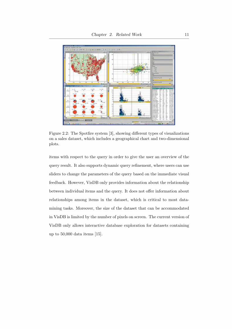
Figure 2.2: The Spotfire system [3], showing different types of visualizationson a sales dataset, which includes a geographical chart and two-dimensionalplots.
items with respect to the query in order to give the user an overview of the
query result. It also supports dynamic query refinement, where users can use
sliders to change the parameters of the query based on the immediate visual
feedback. However, VisDB only provides information about the relationship
between individual items and the query. It does not offer information about
relationships among items in the dataset, which is critical to most data-
mining tasks. Moreover, the size of the dataset that can be accommodated
in VisDB is limited by the number of pixels on screen. The current version of
VisDB only allows interactive database exploration for datasets containing
up to 50,000 data items [15].
Chapter 2. Related Work 12
2.2.1 Spotfire
Spotfire [3], as shown in Figure 2.2, is a database exploration system that em-
ploys several information visualization techniques, including dynamic queries,
brushing and linking, and other interactive graphic techniques. This system
focuses on visualizing the original dataset and uses a graphical interface to
help users identify trends, patterns, and outliers. However, Spotfire does
not provide visualization of any data-mining results. The Spotfire system
also suffers from a lack of scalability and cannot handle databases that are
organized using a hierarchical structure, where users are able to acquire
information with different granularity.
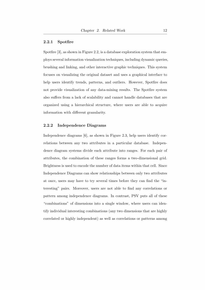
2.2.2 Independence Diagrams
Independence diagrams [6], as shown in Figure 2.3, help users identify cor-
relations between any two attributes in a particular database. Indepen-
dence diagram systems divide each attribute into ranges. For each pair of
attributes, the combination of these ranges forms a two-dimensional grid.
Brightness is used to encode the number of data items within that cell. Since
Independence Diagrams can show relationships between only two attributes
at once, users may have to try several times before they can find the “in-
teresting” pairs. Moreover, users are not able to find any correlations or
pattern among independence diagrams. In contrast, PSV puts all of these
“combinations” of dimensions into a single window, where users can iden-
tify individual interesting combinations (any two dimensions that are highly
correlated or highly independent) as well as correlations or patterns among
Chapter 2. Related Work 13
Figure 2.3: An independence diagram with legend [6], showing a syntheticdataset. Brightness is used to encode degree of dependence. A darker regionmeans that there are fewer items in it. The two attributes are independent,except for a range of X-attribute values, where the region is brighter.
them.
2.2.3 Polaris
Polaris [30, 29], as shown in Figure 2.4, is an interactive visual exploration
tool that facilitates exploratory analysis of multidimensional datasets with
rich hierarchical information. Polaris builds a visual grid of small multi-
ples [31] based on a user query. Polaris also provides a visual interface to
help the user formulate complex queries against a multi-dimensional data
cube. By taking advantage of the hierarchical structure of the data cube,
Polaris allows the analyst to drill down or roll up data to get a complete
overview of the entire dataset before focusing on detailed portions of it. How-
Chapter 2. Related Work 14
Figure 2.4: The Polaris system [30, 29]. Each chart displays profit and salesover time for a hypothetical coffee chain, organized by state.
ever, Polaris is limited to processing basic queries against the data cubes,
and does not support exploring powerset space.
In summary, these four systems provide features for arranging and dis-
playing data in various forms. However, they are not designed to display
data mining results nor could they be easily modified to accommodate pow-
erset enumeration. The PSV system allows the raw data to be visualized
and explored as well as providing a unified visual framework for the user to
examine data-mining results.
Chapter 2. Related Work 15
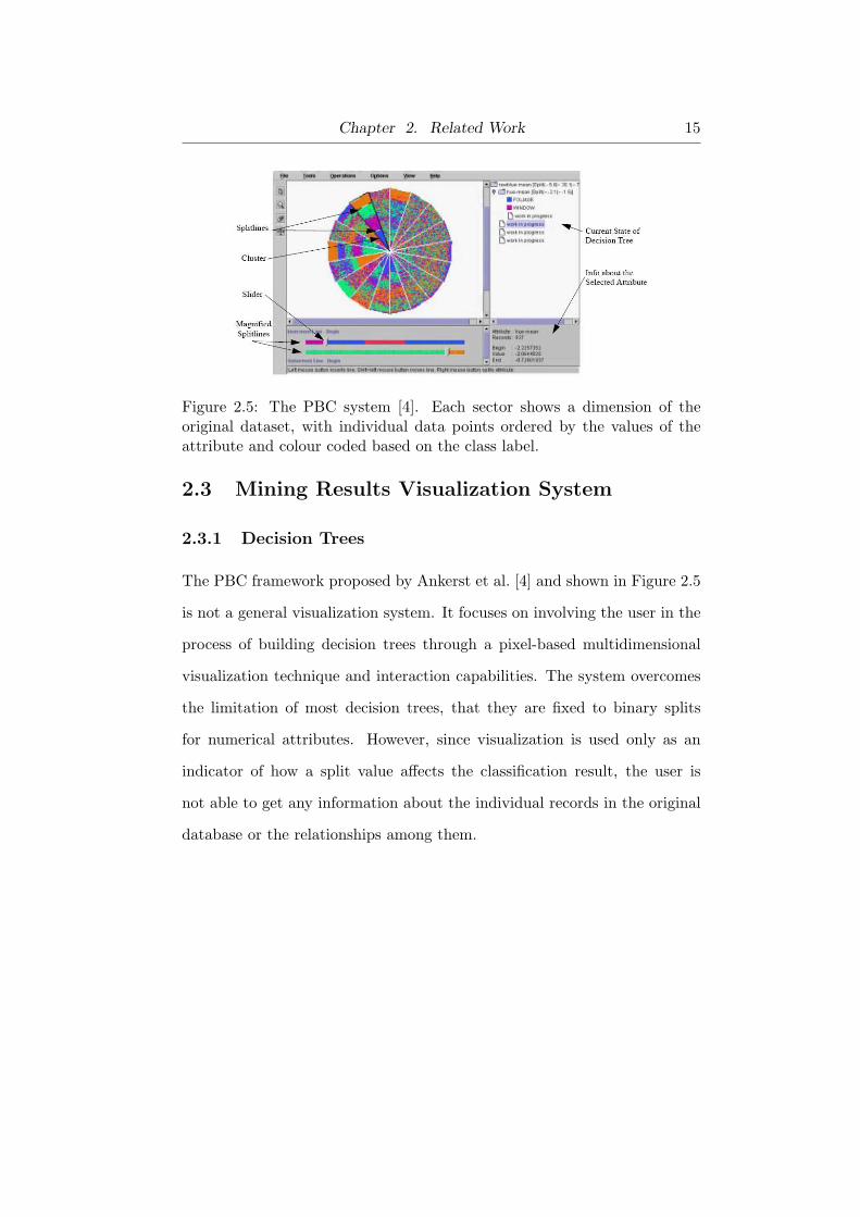
Figure 2.5: The PBC system [4]. Each sector shows a dimension of theoriginal dataset, with individual data points ordered by the values of theattribute and colour coded based on the class label.
2.3 Mining Results Visualization System
2.3.1 Decision Trees
The PBC framework proposed by Ankerst et al. [4] and shown in Figure 2.5
is not a general visualization system. It focuses on involving the user in the
process of building decision trees through a pixel-based multidimensional
visualization technique and interaction capabilities. The system overcomes
the limitation of most decision trees, that they are fixed to binary splits
for numerical attributes. However, since visualization is used only as an
indicator of how a split value affects the classification result, the user is
not able to get any information about the individual records in the original
database or the relationships among them.

Chapter 2. Related Work 16
2.3.2 Association Rules
The rule-visualization system developed by Han and Cercone [11] focuses on
the discretization of numeric attributes and the discovery of the numerical
association rules for large datasets. The system uses a two-dimensional plot
to show the original datasets and parallel coordinates to show the mined
association rules. However, the system takes only two attributes into con-
sideration throughout the mining process. Once a data point is displayed,
users are not able to get detailed information about individual records. In
contrast, PSV allows the user to operate on all attributes of the records.
Hofmann et al. [13] use a variant of mosaic plots, called double-decker
plots, to visualize association rules. Their focus is on helping users to un-
derstand association rules. PowerSetViewer, on the other hand, operates at
the level of frequent sets. Furthermore, unlike the two previous frameworks,
PSV supports midstream steering of the mining process. Again, the use of
a spatial layout based on a powerset is unique.
2.3.3 Clustering
The visualization method developed by Koren and Harel [18] is designed
for clustering analysis and validation. It integrates a dendrogram, which
contains hierarchical information, and low-dimensional embedding. The leaf
nodes of the dendrogram are well ordered so that similar nodes are adjacent
to each other. The data points in the low-dimensional embedding are drawn
exactly below the corresponding leaf node in the dendrogram so that the
user is able to mentally connect the two parts, as shown in Figure 2.6. This

Chapter 2. Related Work 17
system is a specific visualization tool for exploring clusters and provides
no information at the level of individual records. Moreover, the size of the
dendrogram is limited by the number of screen pixels, which limits the utility
of the system.
Figure 2.6: The two-way visualization system for clustered data [18].
The visual metaphors of visualization systems based on data-mining re-
sults are quite different from the PSV system, which uses a spatial layout
based on the powerset of an alphabet. These other systems use dots, lines, or
rectangles to represent data points in the original datasets. These on-screen
elements may overlap with each other when the number of data points ex-
ceeds a certain threshold. However, all of these systems are limited by their
failure to offer elegant solutions to occlusion when laying out large datasets.
Moreover, they do not provide users with the ability to explore the original
datasets.
Chapter 2. Related Work 18
2.4 Steerable Visualization Systems
2.4.1 SCIRun
SCIRun [24] is a scientific programming environment that allows user to
refine parameter settings at any phase of computation, based on the visual
representation of the partial result. It offers users the ability to find the
cause-and-effect relationships within the simulation. However, SCIRun is
designed to provide volumetric representations of the data, such as medical
imaging and scientific simulation, and uses a very different visual represen-
tation than that used by PSV.
2.4.2 MDSteer
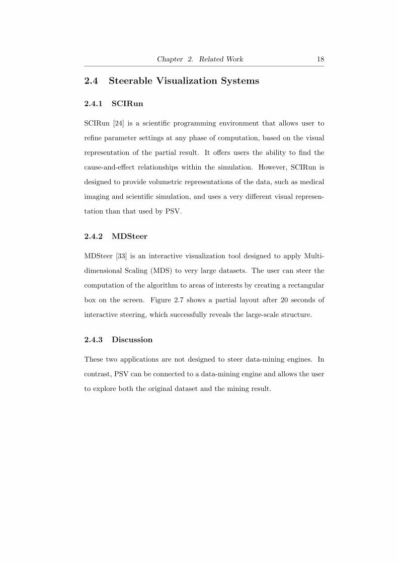
MDSteer [33] is an interactive visualization tool designed to apply Multi-
dimensional Scaling (MDS) to very large datasets. The user can steer the
computation of the algorithm to areas of interests by creating a rectangular
box on the screen. Figure 2.7 shows a partial layout after 20 seconds of
interactive steering, which successfully reveals the large-scale structure.
2.4.3 Discussion
These two applications are not designed to steer data-mining engines. In
contrast, PSV can be connected to a data-mining engine and allows the user
to explore both the original dataset and the mining result.

Chapter 2. Related Work 19
Figure 2.7: The MDSteer system [33], showing a partial layout of a 50, 000-point S-shaped benchmark dataset. Users can steer the computation bycreating boxes.
2.5 Accordion Drawing
Accordion drawing is an information-visualization technique that features
rubber-sheet navigation and guaranteed visibility. Rubber-sheet naviga-
tion allows the user to select and stretch out any rectangular area to show
more detail in that area. This action automatically squishes the rest of the
scene. All stretching and squishing happens with smoothly animated tran-
sitions, so that the user can visually track the motions with ease. Parts of
the scene can become highly compressed, showing very high-level aggregate
views in those regions. However, no part of the scene will ever slide out of
Chapter 2. Related Work 20
the field of view; the borders of the malleable sheet are “nailed down”. A
second critical property of accordion drawing is the guaranteed visibil-
ity of visual landmarks in the scene, even if those features might be much
smaller than a single pixel. Without this guarantee, a user browsing a large
dataset cannot know if an area of the screen is blank because it is truly
empty, or if it is blank because marks in that region happen to be smaller
than the available screen resolution can show.
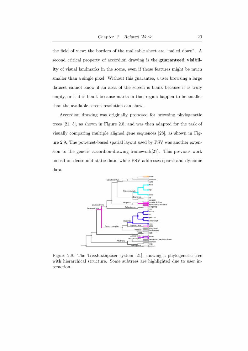
Accordion drawing was originally proposed for browsing phylogenetic
trees [21, 5], as shown in Figure 2.8, and was then adapted for the task of
visually comparing multiple aligned gene sequences [28], as shown in Fig-
ure 2.9. The powerset-based spatial layout used by PSV was another exten-
sion to the generic accordion-drawing framework[27]. This previous work
focusd on dense and static data, while PSV addresses sparse and dynamic
data.
RodentiaRodentiaRodentiaRodentiaRodentiaRodentiaRodentiaRodentiaRodentiaRodentia
mousemousemousemousemousemousemousemousemousemouse
EuarchontogliresEuarchontogliresEuarchontogliresEuarchontogliresEuarchontogliresEuarchontogliresEuarchontogliresEuarchontogliresEuarchontogliresEuarchontoglires
BoreoeutheriaBoreoeutheriaBoreoeutheriaBoreoeutheriaBoreoeutheriaBoreoeutheriaBoreoeutheriaBoreoeutheriaBoreoeutheriaBoreoeutheria
AfrosoricidaAfrosoricidaAfrosoricidaAfrosoricidaAfrosoricidaAfrosoricidaAfrosoricidaAfrosoricidaAfrosoricidaAfrosoricida tenrectenrectenrectenrectenrectenrectenrectenrectenrectenrec
AfrotheriaAfrotheriaAfrotheriaAfrotheriaAfrotheriaAfrotheriaAfrotheriaAfrotheriaAfrotheriaAfrotheria
PerissodactylaPerissodactylaPerissodactylaPerissodactylaPerissodactylaPerissodactylaPerissodactylaPerissodactylaPerissodactylaPerissodactyla
rhinorhinorhinorhinorhinorhinorhinorhinorhinorhino
LaurasiatheriaLaurasiatheriaLaurasiatheriaLaurasiatheriaLaurasiatheriaLaurasiatheriaLaurasiatheriaLaurasiatheriaLaurasiatheriaLaurasiatheria
whalewhalewhalewhalewhalewhalewhalewhalewhalewhale
CetartiodactylaCetartiodactylaCetartiodactylaCetartiodactylaCetartiodactylaCetartiodactylaCetartiodactylaCetartiodactylaCetartiodactylaCetartiodactyla
rousette fruit batrousette fruit batrousette fruit batrousette fruit batrousette fruit batrousette fruit batrousette fruit batrousette fruit batrousette fruit batrousette fruit batChiropteraChiropteraChiropteraChiropteraChiropteraChiropteraChiropteraChiropteraChiropteraChiropteraphyllostomid microbatphyllostomid microbatphyllostomid microbatphyllostomid microbatphyllostomid microbatphyllostomid microbatphyllostomid microbatphyllostomid microbatphyllostomid microbatphyllostomid microbat
rabbitrabbitrabbitrabbitrabbitrabbitrabbitrabbitrabbitrabbitLagomorphaLagomorphaLagomorphaLagomorphaLagomorphaLagomorphaLagomorphaLagomorphaLagomorphaLagomorpha
ruminantruminantruminantruminantruminantruminantruminantruminantruminantruminantllamallamallamallamallamallamallamallamallamallama
tapirtapirtapirtapirtapirtapirtapirtapirtapirtapir
horsehorsehorsehorsehorsehorsehorsehorsehorsehorse
catcatcatcatcatcatcatcatcatcatCarnivoraCarnivoraCarnivoraCarnivoraCarnivoraCarnivoraCarnivoraCarnivoraCarnivoraCarnivora
pangolinpangolinpangolinpangolinpangolinpangolinpangolinpangolinpangolinpangolin
hedgehoghedgehoghedgehoghedgehoghedgehoghedgehoghedgehoghedgehoghedgehoghedgehogEulipotyphlaEulipotyphlaEulipotyphlaEulipotyphlaEulipotyphlaEulipotyphlaEulipotyphlaEulipotyphlaEulipotyphlaEulipotyphlamolemolemolemolemolemolemolemolemolemole
ratratratratratratratratratrat
hystricidhystricidhystricidhystricidhystricidhystricidhystricidhystricidhystricidhystricid
caviomorphcaviomorphcaviomorphcaviomorphcaviomorphcaviomorphcaviomorphcaviomorphcaviomorphcaviomorph
sciuridsciuridsciuridsciuridsciuridsciuridsciuridsciuridsciuridsciurid
flying lemurflying lemurflying lemurflying lemurflying lemurflying lemurflying lemurflying lemurflying lemurflying lemurstrepsirrhinestrepsirrhinestrepsirrhinestrepsirrhinestrepsirrhinestrepsirrhinestrepsirrhinestrepsirrhinestrepsirrhinestrepsirrhinePrimatesPrimatesPrimatesPrimatesPrimatesPrimatesPrimatesPrimatesPrimatesPrimates
slothslothslothslothslothslothslothslothslothslothPilosaPilosaPilosaPilosaPilosaPilosaPilosaPilosaPilosaPilosa
short eared elephant shrewshort eared elephant shrewshort eared elephant shrewshort eared elephant shrewshort eared elephant shrewshort eared elephant shrewshort eared elephant shrewshort eared elephant shrewshort eared elephant shrewshort eared elephant shrewMacroscelideaMacroscelideaMacroscelideaMacroscelideaMacroscelideaMacroscelideaMacroscelideaMacroscelideaMacroscelideaMacroscelidea
aardvarkaardvarkaardvarkaardvarkaardvarkaardvarkaardvarkaardvarkaardvarkaardvarkhyraxhyraxhyraxhyraxhyraxhyraxhyraxhyraxhyraxhyraxopossumopossumopossumopossumopossumopossumopossumopossumopossumopossumMarsupialiaMarsupialiaMarsupialiaMarsupialiaMarsupialiaMarsupialiaMarsupialiaMarsupialiaMarsupialiaMarsupialia
Figure 2.8: The TreeJuxtaposer system [21], showing a phylogenetic treewith hierarchical structure. Some subtrees are highlighted due to user in-teraction.

Chapter 2. Related Work 21
WhaleWhaleWhaleWhaleWhaleWhaleWhaleWhaleWhaleWhale
RuminantRuminantRuminantRuminantRuminantRuminantRuminantRuminantRuminantRuminant
RhinoRhinoRhinoRhinoRhinoRhinoRhinoRhinoRhinoRhino
CatCatCatCatCatCatCatCatCatCat
CaniformCaniformCaniformCaniformCaniformCaniformCaniformCaniformCaniformCaniform
PangolinPangolinPangolinPangolinPangolinPangolinPangolinPangolinPangolinPangolin
Flying_FoxFlying_FoxFlying_FoxFlying_FoxFlying_FoxFlying_FoxFlying_FoxFlying_FoxFlying_FoxFlying_Fox
Rousette_FruitbatRousette_FruitbatRousette_FruitbatRousette_FruitbatRousette_FruitbatRousette_FruitbatRousette_FruitbatRousette_FruitbatRousette_FruitbatRousette_Fruitbat
False_vampire_batFalse_vampire_batFalse_vampire_batFalse_vampire_batFalse_vampire_batFalse_vampire_batFalse_vampire_batFalse_vampire_batFalse_vampire_batFalse_vampire_bat
ShrewShrewShrewShrewShrewShrewShrewShrewShrewShrew
ArmadilloArmadilloArmadilloArmadilloArmadilloArmadilloArmadilloArmadilloArmadilloArmadillo
TenrecidTenrecidTenrecidTenrecidTenrecidTenrecidTenrecidTenrecidTenrecidTenrecid
Golden_MoleGolden_MoleGolden_MoleGolden_MoleGolden_MoleGolden_MoleGolden_MoleGolden_MoleGolden_MoleGolden_Mole
Sh_Ear_Ele_ShrewSh_Ear_Ele_ShrewSh_Ear_Ele_ShrewSh_Ear_Ele_ShrewSh_Ear_Ele_ShrewSh_Ear_Ele_ShrewSh_Ear_Ele_ShrewSh_Ear_Ele_ShrewSh_Ear_Ele_ShrewSh_Ear_Ele_Shrew
Lo_Ear_Ele_shrewLo_Ear_Ele_shrewLo_Ear_Ele_shrewLo_Ear_Ele_shrewLo_Ear_Ele_shrewLo_Ear_Ele_shrewLo_Ear_Ele_shrewLo_Ear_Ele_shrewLo_Ear_Ele_shrewLo_Ear_Ele_shrew
AardvarkAardvarkAardvarkAardvarkAardvarkAardvarkAardvarkAardvarkAardvarkAardvark
TTTTTTTTTT
TTTTTTTTTT
TTTTTTTTTT
TTTTTTTTTT
TTTTTTTTTT
TTTTTTTTTT
TTTTTTTTTT
TTTTTTTTTT
TTTTTTTTTT
TTTTTTTTTT
TTTTTTTTTT
NNNNNNNNNN
TTTTTTTTTT
NNNNNNNNNN
TTTTTTTTTT
TTTTTTTTTT
CCCCCCCCCC
CCCCCCCCCC
CCCCCCCCCC
CCCCCCCCCC
CCCCCCCCCC
CCCCCCCCCC
CCCCCCCCCC
CCCCCCCCCC
CCCCCCCCCC
CCCCCCCCCC
CCCCCCCCCC
NNNNNNNNNN
CCCCCCCCCC
CCCCCCCCCC
CCCCCCCCCC
CCCCCCCCCC
NNNNNNNNNN
CCCCCCCCCC
CCCCCCCCCC
CCCCCCCCCC
CCCCCCCCCC
CCCCCCCCCC
CCCCCCCCCC
CCCCCCCCCC
CCCCCCCCCC
NNNNNNNNNN
CCCCCCCCCC
NNNNNNNNNN
CCCCCCCCCC
CCCCCCCCCC
CCCCCCCCCC
TTTTTTTTTT
TTTTTTTTTT
TTTTTTTTTT
TTTTTTTTTT
TTTTTTTTTT
TTTTTTTTTT
TTTTTTTTTT
TTTTTTTTTT
TTTTTTTTTT
TTTTTTTTTT
TTTTTTTTTT
TTTTTTTTTT
TTTTTTTTTT
TTTTTTTTTT
TTTTTTTTTT
TTTTTTTTTT
TTTTTTTTTT
TTTTTTTTTT
TTTTTTTTTT
TTTTTTTTTT
TTTTTTTTTT
TTTTTTTTTT
TTTTTTTTTT
TTTTTTTTTT
TTTTTTTTTT
TTTTTTTTTT
TTTTTTTTTT
TTTTTTTTTT
TTTTTTTTTT
TTTTTTTTTT
TTTTTTTTTT
TTTTTTTTTT
TTTTTTTTTT
AAAAAAAAAA
AAAAAAAAAA
AAAAAAAAAA
AAAAAAAAAA
AAAAAAAAAA
AAAAAAAAAA
AAAAAAAAAA
AAAAAAAAAA
AAAAAAAAAA
AAAAAAAAAA
AAAAAAAAAA
AAAAAAAAAA
TTTTTTTTTT
AAAAAAAAAA
AAAAAAAAAA
AAAAAAAAAA
GGGGGGGGGG
GGGGGGGGGG
GGGGGGGGGG
GGGGGGGGGG
GGGGGGGGGG
GGGGGGGGGG
GGGGGGGGGG
GGGGGGGGGG
GGGGGGGGGG
GGGGGGGGGG
GGGGGGGGGG
GGGGGGGGGG
GGGGGGGGGG
GGGGGGGGGG
GGGGGGGGGG
GGGGGGGGGG
GGGGGGGGGG
GGGGGGGGGG
GGGGGGGGGG
AAAAAAAAAA
GGGGGGGGGG
GGGGGGGGGG
GGGGGGGGGG
GGGGGGGGGG
GGGGGGGGGG
GGGGGGGGGG
GGGGGGGGGG
GGGGGGGGGG
AAAAAAAAAA
AAAAAAAAAA
AAAAAAAAAA
GGGGGGGGGG
GGGGGGGGGG
GGGGGGGGGG
GGGGGGGGGG
GGGGGGGGGG
GGGGGGGGGG
GGGGGGGGGG
GGGGGGGGGG
GGGGGGGGGG
GGGGGGGGGG
GGGGGGGGGG
GGGGGGGGGG
GGGGGGGGGG
GGGGGGGGGG
GGGGGGGGGG
GGGGGGGGGG
GGGGGGGGGG
AAAAAAAAAA
GGGGGGGGGG
GGGGGGGGGG
AAAAAAAAAA
AAAAAAAAAA
GGGGGGGGGG
AAAAAAAAAA
AAAAAAAAAA
AAAAAAAAAA
AAAAAAAAAA
AAAAAAAAAA
AAAAAAAAAA
AAAAAAAAAA
AAAAAAAAAA
AAAAAAAAAA
AAAAAAAAAA
TTTTTTTTTT
TTTTTTTTTT
TTTTTTTTTT
TTTTTTTTTT
TTTTTTTTTT
TTTTTTTTTT
TTTTTTTTTT
TTTTTTTTTT
TTTTTTTTTT
TTTTTTTTTT
GGGGGGGGGG
TTTTTTTTTT
GGGGGGGGGG
AAAAAAAAAA
TTTTTTTTTT
TTTTTTTTTT
AAAAAAAAAA
AAAAAAAAAA
AAAAAAAAAA
AAAAAAAAAA
AAAAAAAAAA
AAAAAAAAAA
AAAAAAAAAA
AAAAAAAAAA
AAAAAAAAAA
AAAAAAAAAA
AAAAAAAAAA
AAAAAAAAAA
AAAAAAAAAA
AAAAAAAAAA
AAAAAAAAAA
AAAAAAAAAA
CCCCCCCCCC
CCCCCCCCCC
CCCCCCCCCC
CCCCCCCCCC
CCCCCCCCCC
CCCCCCCCCC
CCCCCCCCCC
CCCCCCCCCC
CCCCCCCCCC
CCCCCCCCCC
CCCCCCCCCC
CCCCCCCCCC
CCCCCCCCCC
CCCCCCCCCC
TTTTTTTTTT
CCCCCCCCCC
CCCCCCCCCC
NNNNNNNNNN
CCCCCCCCCC
CCCCCCCCCC
CCCCCCCCCC
CCCCCCCCCC
AAAAAAAAAA
CCCCCCCCCC
CCCCCCCCCC
CCCCCCCCCC
GGGGGGGGGG
NNNNNNNNNN
CCCCCCCCCC
AAAAAAAAAA
AAAAAAAAAA
NNNNNNNNNN
GGGGGGGGGG
NNNNNNNNNN
TTTTTTTTTT
TTTTTTTTTT
TTTTTTTTTT
TTTTTTTTTT
TTTTTTTTTT
TTTTTTTTTT
TTTTTTTTTT
GGGGGGGGGG
GGGGGGGGGG
NNNNNNNNNN
TTTTTTTTTT
TTTTTTTTTT
TTTTTTTTTT
NNNNNNNNNN
GGGGGGGGGG
NNNNNNNNNN
GGGGGGGGGG
GGGGGGGGGG
GGGGGGGGGG
GGGGGGGGGG
GGGGGGGGGG
GGGGGGGGGG
GGGGGGGGGG
GGGGGGGGGG
GGGGGGGGGG
NNNNNNNNNN
GGGGGGGGGG
GGGGGGGGGG
GGGGGGGGGG
NNNNNNNNNN
CCCCCCCCCC
NNNNNNNNNN
GGGGGGGGGG
GGGGGGGGGG
GGGGGGGGGG
GGGGGGGGGG
CCCCCCCCCC
GGGGGGGGGG
GGGGGGGGGG
GGGGGGGGGG
GGGGGGGGGG
NNNNNNNNNN
GGGGGGGGGG
GGGGGGGGGG
CCCCCCCCCC
NNNNNNNNNN
TTTTTTTTTT
TTTTTTTTTT
NNNNNNNNNN
TTTTTTTTTT
TTTTTTTTTT
NNNNNNNNNN
TTTTTTTTTT
TTTTTTTTTT
NNNNNNNNNN
TTTTTTTTTT
TTTTTTTTTT
TTTTTTTTTT
NNNNNNNNNN
TTTTTTTTTT
NNNNNNNNNN
TTTTTTTTTT
CCCCCCCCCC
CCCCCCCCCC
AAAAAAAAAA
AAAAAAAAAA
AAAAAAAAAA
AAAAAAAAAA
AAAAAAAAAA
AAAAAAAAAA
AAAAAAAAAA
CCCCCCCCCC
AAAAAAAAAA
CCCCCCCCCC
AAAAAAAAAA
CCCCCCCCCC
TTTTTTTTTT
AAAAAAAAAA
CCCCCCCCCC
GGGGGGGGGG
AAAAAAAAAA
GGGGGGGGGG
GGGGGGGGGG
AAAAAAAAAA
AAAAAAAAAA
AAAAAAAAAA
AAAAAAAAAA
GGGGGGGGGG
AAAAAAAAAA
AAAAAAAAAA
AAAAAAAAAA
AAAAAAAAAA
GGGGGGGGGG
AAAAAAAAAA
CCCCCCCCCC
CCCCCCCCCC
TTTTTTTTTT
AAAAAAAAAA
AAAAAAAAAA
AAAAAAAAAA
AAAAAAAAAA
AAAAAAAAAA
AAAAAAAAAA
TTTTTTTTTT
TTTTTTTTTT
CCCCCCCCCC
AAAAAAAAAA
AAAAAAAAAA
TTTTTTTTTT
TTTTTTTTTT
TTTTTTTTTT
TTTTTTTTTT
TTTTTTTTTT
TTTTTTTTTT
TTTTTTTTTT
TTTTTTTTTT
TTTTTTTTTT
TTTTTTTTTT
TTTTTTTTTT
TTTTTTTTTT
TTTTTTTTTT
TTTTTTTTTT
TTTTTTTTTT
TTTTTTTTTT
TTTTTTTTTT
TTTTTTTTTT
GGGGGGGGGG
GGGGGGGGGG
GGGGGGGGGG
GGGGGGGGGG
GGGGGGGGGG
TTTTTTTTTT
TTTTTTTTTT
TTTTTTTTTT
GGGGGGGGGG
GGGGGGGGGG
GGGGGGGGGG
GGGGGGGGGG
GGGGGGGGGG
GGGGGGGGGG
GGGGGGGGGG
TTTTTTTTTT
AAAAAAAAAA
AAAAAAAAAA
AAAAAAAAAA
AAAAAAAAAA
AAAAAAAAAA
AAAAAAAAAA
AAAAAAAAAA
AAAAAAAAAA
AAAAAAAAAA
CCCCCCCCCC
AAAAAAAAAA
CCCCCCCCCC
AAAAAAAAAA
CCCCCCCCCC
CCCCCCCCCC
AAAAAAAAAA
CCCCCCCCCC
CCCCCCCCCC
CCCCCCCCCC
CCCCCCCCCC
CCCCCCCCCC
CCCCCCCCCC
CCCCCCCCCC
CCCCCCCCCC
CCCCCCCCCC
CCCCCCCCCC
TTTTTTTTTT
CCCCCCCCCC
CCCCCCCCCC
CCCCCCCCCC
CCCCCCCCCC
CCCCCCCCCC
CCCCCCCCCC
CCCCCCCCCC
CCCCCCCCCC
CCCCCCCCCC
CCCCCCCCCC
CCCCCCCCCC
CCCCCCCCCC
CCCCCCCCCC
CCCCCCCCCC
CCCCCCCCCC
CCCCCCCCCC
CCCCCCCCCC
CCCCCCCCCC
CCCCCCCCCC
CCCCCCCCCC
CCCCCCCCCC
CCCCCCCCCC
CCCCCCCCCC
CCCCCCCCCC
CCCCCCCCCC
CCCCCCCCCC
CCCCCCCCCC
CCCCCCCCCC
CCCCCCCCCC
CCCCCCCCCC
CCCCCCCCCC
CCCCCCCCCC
CCCCCCCCCC
TTTTTTTTTT
TTTTTTTTTT
TTTTTTTTTT
CCCCCCCCCC
CCCCCCCCCC
CCCCCCCCCC
CCCCCCCCCC
CCCCCCCCCC
CCCCCCCCCC
CCCCCCCCCC
NNNNNNNNNN
CCCCCCCCCC
CCCCCCCCCC
CCCCCCCCCC
CCCCCCCCCC
CCCCCCCCCC
TTTTTTTTTT
CCCCCCCCCC
CCCCCCCCCC
TTTTTTTTTT
GGGGGGGGGG
GGGGGGGGGG
GGGGGGGGGG
GGGGGGGGGG
GGGGGGGGGG
GGGGGGGGGG
GGGGGGGGGG
GGGGGGGGGG
GGGGGGGGGG
CCCCCCCCCC
GGGGGGGGGG
GGGGGGGGGG
CCCCCCCCCC
GGGGGGGGGG
GGGGGGGGGG
GGGGGGGGGG
TTTTTTTTTT
TTTTTTTTTT
TTTTTTTTTT
AAAAAAAAAA
TTTTTTTTTT
AAAAAAAAAA
AAAAAAAAAA
AAAAAAAAAA
TTTTTTTTTT
TTTTTTTTTT
TTTTTTTTTT
TTTTTTTTTT
TTTTTTTTTT
TTTTTTTTTT
TTTTTTTTTT
TTTTTTTTTT
GGGGGGGGGG
CCCCCCCCCC
GGGGGGGGGG
CCCCCCCCCC
GGGGGGGGGG
GGGGGGGGGG
GGGGGGGGGG
CCCCCCCCCC
GGGGGGGGGG
GGGGGGGGGG
CCCCCCCCCC
CCCCCCCCCC
GGGGGGGGGG
GGGGGGGGGG
CCCCCCCCCC
GGGGGGGGGG
AAAAAAAAAA
AAAAAAAAAA
AAAAAAAAAA
AAAAAAAAAA
AAAAAAAAAA
AAAAAAAAAA
AAAAAAAAAA
AAAAAAAAAA
AAAAAAAAAA
AAAAAAAAAA
AAAAAAAAAA
AAAAAAAAAA
AAAAAAAAAA
NNNNNNNNNN
AAAAAAAAAA
AAAAAAAAAA
AAAAAAAAAA
AAAAAAAAAA
AAAAAAAAAA
AAAAAAAAAA
AAAAAAAAAA
AAAAAAAAAA
AAAAAAAAAA
AAAAAAAAAA
AAAAAAAAAA
AAAAAAAAAA
AAAAAAAAAA
AAAAAAAAAA
AAAAAAAAAA
NNNNNNNNNN
AAAAAAAAAA
AAAAAAAAAA
AAAAAAAAAA
AAAAAAAAAA
AAAAAAAAAA
AAAAAAAAAA
AAAAAAAAAA
AAAAAAAAAA
AAAAAAAAAA
AAAAAAAAAA
AAAAAAAAAA
AAAAAAAAAA
AAAAAAAAAA
AAAAAAAAAA
AAAAAAAAAA
NNNNNNNNNN
AAAAAAAAAA
AAAAAAAAAA
GGGGGGGGGG
GGGGGGGGGG
NNNNNNNNNN
GGGGGGGGGG
CCCCCCCCCC
GGGGGGGGGG
GGGGGGGGGG
NNNNNNNNNN
CCCCCCCCCC
CCCCCCCCCC
NNNNNNNNNN
NNNNNNNNNN
NNNNNNNNNN
NNNNNNNNNN
GGGGGGGGGG
GGGGGGGGGG
CCCCCCCCCC
CCCCCCCCCC
NNNNNNNNNN
CCCCCCCCCC
CCCCCCCCCC
CCCCCCCCCC
CCCCCCCCCC
NNNNNNNNNN
CCCCCCCCCC
CCCCCCCCCC
NNNNNNNNNN
NNNNNNNNNN
NNNNNNNNNN
CCCCCCCCCC
NNNNNNNNNN
CCCCCCCCCC
CCCCCCCCCC
CCCCCCCCCC
CCCCCCCCCC
CCCCCCCCCC
CCCCCCCCCC
CCCCCCCCCC
CCCCCCCCCC
CCCCCCCCCC
CCCCCCCCCC
CCCCCCCCCC
CCCCCCCCCC
CCCCCCCCCC
AAAAAAAAAA
CCCCCCCCCC
NNNNNNNNNN
AAAAAAAAAA
AAAAAAAAAA
AAAAAAAAAA
AAAAAAAAAA
AAAAAAAAAA
AAAAAAAAAA
AAAAAAAAAA
AAAAAAAAAA
AAAAAAAAAA
AAAAAAAAAA
AAAAAAAAAA
AAAAAAAAAA
AAAAAAAAAA
AAAAAAAAAA
AAAAAAAAAA
AAAAAAAAAA
AAAAAAAAAA
Figure 2.9: The SequenceJuxtaposer system [28], showing a set of relatedgene sequences. These sequences are vertically aligned for easy comparison.
22
Chapter 3
PSV Overview
In this chapter, we give a detailed overview of our approach. Sections 3.1.1
through 3.1.4 explain the features that are supported by our system. Sec-
tion 3.2 explains the client-server architecture of PSV. Finally, Section 3.3
introduces PSVproto, an initial prototype, and its limitations.
3.1 Features
PSV provides a visual framework for examining individual powersets in
the context of the entire powerset space, and also an interface where users
can find appropriate parameter settings for data-mining algorithms through
lightweight visual experimentation that shows partial results. This light-
weight visual experimentation also shows how various parameter settings
would create a filter for the mined data with respect to the entire dataset.
Moreover, when the mining algorithms are steerable, dynamic display of
intermediate or partial results helps the user decide how to change the pa-
rameters settings of computation in midstream. In our unified framework,
we can support setting the filter parameters to let all items pass through,
so that the entire input dataset is shown to the user. Another benefit of
using the powerset for spatial layout is that users can meaningfully compare

Chapter 3. PSV Overview 23
images that represent two different datasets sharing the same alphabet. For
example, the distribution of purchases between two chain stores in different
geographic regions could be compared this way. Our system provides the
following features to assist users with frequent-set mining.
3.1.1 Visual Metaphor
PSV uses the visual metaphor of accordion drawing [27] introduced in
Section 2.5. Although the absolute on-screen location of an itemset changes,
its relative ordering with respect to its neighbours is always preserved in
both the horizontal and vertical directions. Accordion drawing also allows
interactive exploration of datasets that contain many more itemsets than
the fixed number of pixels available in a finite display.
3.1.2 Layout
PSV introduces a novel layout that maps a related family of datasets, those
sharing the same alphabet of available items, into the same absolute space of
all possibilities. That space is created by enumerating the entire powerset of
a finite alphabet as a very long one-dimensional list, where every possible set
has an index in that list. The linear list is wrapped scanline-style to create
a two-dimensional rectangular grid of fixed width, with a small number of
columns and a very large number of rows. We draw a small box representing
a set if it is passed to the visualizer by the miner, located at the position in
the grid corresponding to its index in this wrapped enumeration list. With-
out guaranteed visibility, these boxes would be much smaller than pixels in
the display for alphabets of any significant size because of the exponential
Chapter 3. PSV Overview 24
nature of the powerset. This guarantee is one fundamental reason why PSV
can handle large alphabets.
In areas where there is not enough room to draw one box for each set,
multiple sets are represented by a single aggregate box. The colour of this
box is a visual encoding of the number of sets that it represents using satu-
ration: objects representing few sets are pale, and those representing many
are dark and fully saturated. Colour is also used in the background to dis-
tinguish between areas where sets of different cardinality are drawn: those
background regions alternate between four unobtrusive, unsaturated colours.
The minimum size of boxes is controllable, from a minimum of one pixel to
a maximum of large blocks that are legible even on high-resolution displays.
In this layout, seeing visual patterns in the same relative spatial region in
the visualization of two different datasets means that they have similarities
in their distribution in this absolute powerset space. Side by side visual
comparison of two different datasets sharing the same alphabet is thus a
fruitful endeavor.
3.1.3 Interaction
Interactions that can be accomplished quickly and easily allow more fluid ex-
ploration than those that require significant effort and time to carry out. The
PSV design philosophy is that simple operations should only require mini-
mal interaction overhead. Rubber-sheet navigation, where the user sweeps
out a box anywhere in the display and then drags the corner of the box
to stretch or shrink it, is just one example. Mouseover highlighting occurs
whenever the cursor is moved, so that the box currently under the cursor
Chapter 3. PSV Overview 25
is highlighted and the names of the items in that highlighted itemset are
shown in a status line below the display. Mouseover highlighting is a very
fast operation that can be carried out many times each second because it
does not require redrawing the entire scene. Highlighting the superset of an
itemset can be done through the shortcut of a single click on the itemset’s
box.
The layout and rubber-sheet navigation described above provide a spatial
substrate users can explore on by colouring sets according to constraints. We
do not support changes in the relative spatial position of itemsets, because
it would then be impossible to usefully compare visual patterns at different
times during the interaction. The underlying mechanism for colouring is to
assign sets to a group that has an assignable colour. A group is a collection of
sets that satisfy certain constraints. Users can create an arbitrary number of
coloured groups as a mechanism for tracking the history of both visualizer
and miner constraints, by saving each interesting constraint choice as a
separate group. The priority of groups is controllable by the user; when a
particular set belongs to multiple enabled groups, the highest priority group
colour is shown.
3.1.4 Monitoring
As will be discussed in Chapter 5, the visualizer shows several important
status variables, which helps the user to adjust parameter settings. These
include the following:
• Total: The total number of itemsets in the raw dataset
Chapter 3. PSV Overview 26
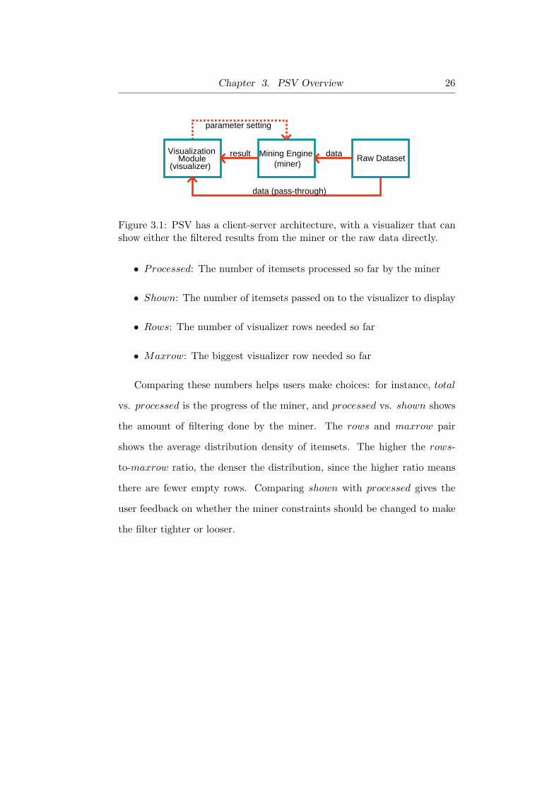
VisualizationModule
(visualizer)
Mining Engine(miner)
Raw Datasetresult data
data (pass-through)
parameter setting
Figure 3.1: PSV has a client-server architecture, with a visualizer that canshow either the filtered results from the miner or the raw data directly.
• Processed: The number of itemsets processed so far by the miner
• Shown: The number of itemsets passed on to the visualizer to display
• Rows: The number of visualizer rows needed so far
• Maxrow: The biggest visualizer row needed so far
Comparing these numbers helps users make choices: for instance, total
vs. processed is the progress of the miner, and processed vs. shown shows
the amount of filtering done by the miner. The rows and maxrow pair
shows the average distribution density of itemsets. The higher the rows-
to-maxrow ratio, the denser the distribution, since the higher ratio means
there are fewer empty rows. Comparing shown with processed gives the
user feedback on whether the miner constraints should be changed to make
the filter tighter or looser.
Chapter 3. PSV Overview 27
3.2 Client-Server Architecture
PSV has a client-server architecture, as shown in Figure 3.1. The server is a
steerable data-mining engine, the miner, that is connected through sockets
with a client visualization module, the visualizer, that handles graphical
display. The visualizer client includes interface components for controlling
both itself and the miner server. The client and server communicate using
a simple text protocol: the client sends control messages to the server. The
miner sends partial results to the visualizer as they are completed, allowing
the user to monitor progress.
3.3 PSVproto
PSVproto, an initial prototype of PSV, had been implemented when the
research for this thesis began. The server-side mining engine was first devel-
oped by Carson Leung and was then modified by Dragana Radulovic so that
the engine could communicate with the visualizer through plain text proto-
col. The client-side of PSVproto was developed by Jordan Lee. Figure 3.4
shows the original PSVproto interface. The top section is the rendering
window, which supports Accordion Drawing navigation. The lower control
panel allows users to communicate with the data-mining engine. In addition
to the main control panel and rendering window, PSVproto also provides
users with the following panels:
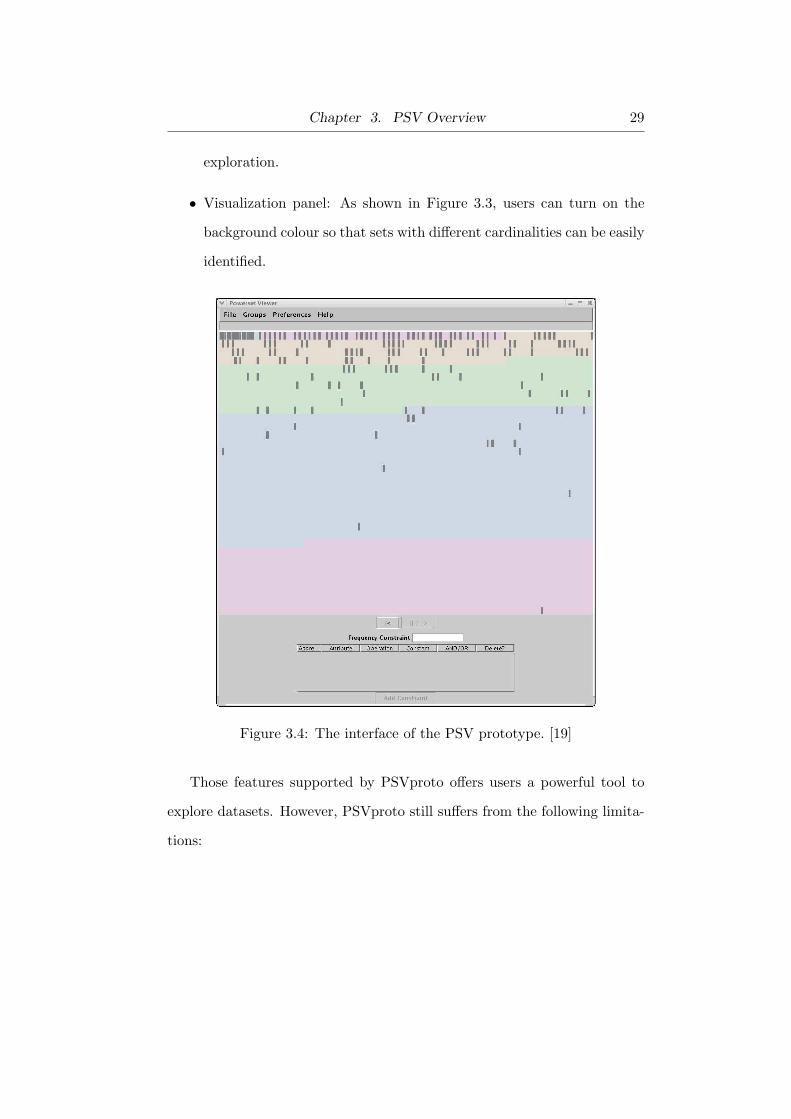
• Grouping panel: As shown in Figure 3.2, users can select a group of
items satisfying the supplied constraints and highlight them for further

Chapter 3. PSV Overview 28
Figure 3.2: The grouping panel of PSVproto. [19]
Figure 3.3: The visualization panel of PSVproto. [19]
Chapter 3. PSV Overview 29
exploration.
• Visualization panel: As shown in Figure 3.3, users can turn on the
background colour so that sets with different cardinalities can be easily
identified.
Figure 3.4: The interface of the PSV prototype. [19]
Those features supported by PSVproto offers users a powerful tool to
explore datasets. However, PSVproto still suffers from the following limita-
tions:

Chapter 3. PSV Overview 30
• Enumeration: The prototype uses a brute-force algorithm to calcu-
late the index of a set in the entire powerset enumeration. Given a set
s, the algorithm traverses the powerset space from the very beginning
of the enumeration until it encounters s. On average, computing the
index of a set takes 40 milliseconds with this approach. Since the op-
eration is performed every time a set comes into PSVproto, it is not
ideal for processing very large datasets.
• Scalability: The PSV prototype cannot display a dataset with an
alphabet size larger than 30 items [19]. Since the PSV prototype uses
the plain Integer type variable as the index of a set in the power-
set enumeration, the size of the alphabet is in turn limited by the
maximum value of the Integer, which is 231.
• Rendering: Since the PSV prototype cannot handle a dataset with an
alphabet size larger than 30 items, rendering is not efficient. The PSV
prototype employs a quad-tree data structure. A quad-tree is very
similar to a binary tree, but any node in a quad-tree can contain up to
four children. The quad-tree maintains a hierarchical structure of the
rendering window, where each leaf node corresponds to a set returned
by the server. Since we subdivide the screen as we are traversing from
the root to a leaf node, a large portion of the screen space will not be
used, since the distribution of the sets is extremely sparse. Therefore,
quad-tree is not an ideal data structure for rendering any mid-size
or large-size datasets. Moreover, it takes PSVproto half a second to
render a scene that contains only a few thousand items.

Chapter 3. PSV Overview 31
The aforementioned limitations of PSVproto makes it unsuitable for process-
ing most real-world datasets, whose alphabet sizes exceed its limit of 30
items. In the next chapter, we will explain how PSV is designed to over-
come these limitations.
32
Chapter 4
Approach
As discussed in Chapter 3, our approach can be divided into three parts.
The first part is to map each set to a box on the display, where the relative
positions of the sets should be maintained. The second part is to build and
maintain related data structures to support fast rendering and navigation.
The last part is to render the sets on screen. In this chapter, we discuss these
three parts in detail in sections 4.1 to section 4.3 respectively. In section 4.4,
we explain how PSV is designed to handle datasets with large alphabets.
4.1 Mapping
Mapping is the process of finding the position of a set in the enumeration
of powersets and using an on-screen box to represent it, so that the relative
position of the set with respect to other sets is maintained.
4.1.1 Challenges
A meaningful ordering of the powerset is critical to the data-mining task,
because useful hidden patterns will be made available if a meaningful or-
dering of the powerset is chosen. Moreover, each set that comes into PSV
will go through the mapping process. Therefore, an appropriate yet efficient
Chapter 4. Approach 33
algorithm is required to map each set to a position on the screen.
4.1.2 Our Approach
There are many ways to enumerate powersets, but when visually represented
most do not yield a helpful mental model. The enumeration we use is or-
dered first by cardinality, then by lexicographic ordering. All singleton sets
are shown before the two-sets, two-sets before the three-sets, and so on.
The steerable data-mining engine that motivated this application uses an
underlying lattice structure, so first sorting by cardinality is a good match.
Within a given cardinality, we choose a lexicographic ordering for alphabet
items, again to match the powerset traversal order of many lattice-based
mining algorithms. For example, an alphabet of {a,b,. . .,z} yields the enu-
meration {a}, {b}, . . ., {z}, {ab}, {ac}, . . ., {yz}, {abc}, . . .. We
assume that the underlying alphabet has a canonical lexicographic order-
ing; for example, a = 1, b = 2, . . . , z = 26. Another design guideline was to
choose a single spatial layout and allow users to find patterns by changing
the colours of data elements. If we used spatial proximity to show mem-
bership of some chosen element, for example by grouping sets containing
the element b, the layout would change drastically and visual patterns from
different times could not be meaningfully compared. Rubber-sheet naviga-
tion can change the absolute position of boxes in space while preserving the
relative ordering of marks in all directions. All computations involving sets
assume that their internal item ordering is also lexicographically sorted.
The mapping from a set to a box that is drawn in a display window has
two main steps:

Chapter 4. Approach 34
• convert from an m-set {s1, . . . , sm} to its index e in the enumeration
of the powerset
• convert from the enumeration index e to a (row, column) position in
the grid of boxes
We present an efficient O(m) algorithm for the first stage of computing
an enumeration index e given an arbitrary set. The second stage is straight-
forward: row is e divided by the width of the grid, and column is e modulo
the width. We start with an example of computing the enumeration index
e = 1206 of the 3-set {d,h,k} given an alphabet of size 26.
Given a particular m-set, the computation of the index in the enu-
meration of the powerset is done in two steps. The first step is to com-
pute the total number of k-sets, for all k < m. These are all the sets
with a strictly smaller cardinality. For the {d,h,k} example, the first step
is to compute the total number of 1-sets and 2-sets, which is given by(26
1
)+
(262
)= 26 + 325 = 315. The general formula, where A is the size
of the alphabet, ism−1∑
i=1
(A
i
).
The second step is to compute the the number of sets between the first m-
set in the enumeration and the particular m-set of interest. For the {d,h,k}example, the second step computes three terms:
• the number of 3-sets beginning with the 1-prefixes {a}, {b}, or {c}:(26−1
2
)+
(26−22
)+
(26−32
)= 300 + 276 + 253 = 829. Picking a as a 1-
prefix leaves 2 other choices that yield a 3-set containing a; there are
25 other items left in the alphabet from which to choose 2. Similarly,

Chapter 4. Approach 35
when b is then picked as the 1-prefix, there are only 24 choices left;
since the m-set is internally ordered lexicographically, neither a nor b
is still available as a choice.
• the number of 3-sets beginning with 2-prefixes {d,e}, {d,f}, or {d,g},which is given by
(26−51
)+
(26−61
)+
(26−71
)= 21 + 20 + 19 = 60; and
• the number of 3-sets between the 3-prefixes {d,h,i} and {d,h,j},which is
(26−90
)+
(26−100
)= 1 + 1 = 2.
This example suggests a formula of
m∑
i=1
pi−1∑
j=pi−1+1
(A− j
m− i
)
where pi is the lexicographic index of the ith element of the m-set and p0 is
0. In the worst case, the number of terms required to compute this sum is
linear in the size of the alphabet. However, we can collapse the inner sum
to be just two terms by noticing that
j∑
i=0
(n− i
k
)=
(n + 1k + 1
)−
(n− j
k + 1
).
We derive this lemma using the identity(nk
)=
(n−1k
)+
(n−1k−1
). The general
formula is thus given by
m∑
i=1
[(A− pi−1
m− i + 1
)−
(A− pi + 1m− i + 1
)](4.1)
Combining these two steps, we can compute the enumeration index as
m−1∑
i=1
(A
i
)+
m∑
i=1
[(A− pi−1
m− i + 1
)−
(A− pi + 1m− i + 1
)](4.2)

Chapter 4. Approach 36
The complexity of computing the index of a set can be reduced to O(m),
where m is the cardinality of the set, by using a lookup table instead of ex-
plicitly calculating(nk
). We compute such a table of size n×k using dynamic
programming in a preprocessing step. As we will discuss in Section 4.4.2, the
maximum set size k needed for these computations is often much less than
the alphabet size n, but we do not want to hardwire any specific limit on
maximum set size. Our time-space tradeoff is to use the lookup table for the
common case of small k, 25 in our current implementation, and explicitly
compute the binomial coefficient for the rare case of a large k.
4.1.3 Knuth’s Algorithm
As discussed in Section 4.1.1, an efficient enumeration algorithm yielding a
meaningful visualization is essential to PSV. In this section, we present an
alternative enumeration algorithm proposed by Donald E. Knuth to explore
the possibilities of employing different enumeration methods in PSV [16].
We will compare Knuth’s approach with ours in terms of both complexity
and usefulness.
Knuth’s algorithm uses the following formula to calculate the index of
an arbitrary m-set in the powerset enumeration:
m−1∑
i=1
(A
i
)+
m∑
i=1
(pi − 1
i
)(4.3)
where A is the size of the alphabet and pi is the lexicographic index of the
ith element of the m-set [16] 1. This algorithm has the same complexity as1Background material for this approach is discussed in Volume 4 of The Art of Com-
puter Programming [17]

Chapter 4. Approach 37
Figure 4.1: Two visualizations with different enumeration functions. Topvisualization uses our approach while bottom one uses Knuth’s algorithm.These two enumeration methods give very similar distributions.

Chapter 4. Approach 38
ours but the resulting enumeration does not strictly follow the lexicographic
order. For example, given an alphabet of {a,b,c,d,e}, the set {b,c,d}comes before {a,b,e}. However, this enumeration has a nice property: any
m-set that contains ai comes after all m-sets that are generated using {a1,
a2, . . ., ai−1}, where ai is the ith element in the alphabet. This process
is especially useful when the alphabet size keeps increasing over time, since
the newly generated powersets will be appended at the end of the powerset
enumeration, leaving the layout of the exiting sets untouched. As shown in
Figure 4.1, Knuth’s approach and ours give two very similar visualizations
of the enrollment dataset, which will be introduced in Section 5.1.
4.2 SplitLine Hierarchy
Once the index in the enumeration of an itemset has been calculated, we
need to create boundaries, which we discuss next.
4.2.1 Challenges
All itemsets will be laid out in a 2-D grid, where each box that represents
an itemset is bounded by four movable lines, which we call SplitLines.
Rubber-sheet navigation is accomplished by moving the SplitLines. The full
powerset space is extremely large. For example, for a database that has
an alphabet size of 50 items, the total number of powersets is 1.12 × 10¹⁵,
which, considering the memory requirements, makes it impossible to create
all SplitLines beforehand. Moreover, for alphabets of any significant size,
the screen space allocated to each of the boxes would be much smaller than a

Chapter 4. Approach 39
pixel in the display because of the cardinality of the powerset. To guarantee
visibility, we need to maintain some aggregation information for use by the
rendering engine at the rendering stage.
4.2.2 Our Approach
As shown in Figure 4.2 Left, SplitLines are boundaries of boxes that are to be
rendered on the display. All boxes in the same row share the same upper and
lower SplitLines. Two adjacent rows also share a SplitLine that lies between
the two rows. The column case is analogous. Users are able to change the
size of part of the screen by dragging SplitLines that are boundaries of that
region. As shown in Figure 4.2 Right, after the second vertical SplitLine is
dragged to the left, the region to the left of it is squished, while the size of
the region on the right side of the third vertical SplitLine remains the same.
Figure 4.2: Left : boxes are bounded by SplitLines. Screen space is evenlydistributed before dragging. Right : the region occupied by the red boxgrows bigger by dragging the second vertical SplitLine left and the secondhorizontal SplitLine up.
A set of SplitLines provides both a linear ordering and a hierarchical
Chapter 4. Approach 40
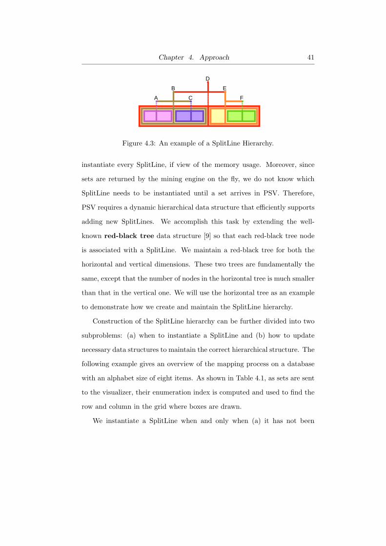
subdivision of space, as shown in Figure 4.3. Linearly, SplitLine B falls
spatially between A and C. Hierarchically, it splits the region to the left of
its parent SplitLine D in two, and its range is from the minimum SplitLine
to the maximum of its parent SplitLine D. The diagram here shows only
the vertical SplitLines; the horizontal situation is analogous. Each SplitLine
has a split value, which ranges from 0 to 1. This value indicates the relative
position of the SplitLine with respect to the boundary.
Rendering the boxes in the correct position on the display requires cal-
culating the absolute positions of SplitLines. PRISAD [27] is a generic
rendering infrastructure for information visualization applications on top of
which PSV is built. It makes use of a hierarchical structure to organize the
SplitLines to support efficient calculation of their absolute positions on the
fly. When calculating the absolute value of a SplitLine, PRISAD simply
traverses the SplitLine hierarchy from the root to the node that represents
that SplitLine. The complexity of this operation is bounded by the depth
of the tree, which is efficient enough to support real-time interaction.
Construction and maintenance are the two major tasks related to the
SplitLine hierarchy. PRISAD is responsible for maintaining the correct hi-
erarchical information once the SplitLine hierarchy has been successfully
constructed. For example, after navigation by a user, PRISAD will update
the split values when necessary to reflect the user’s interaction. Detailed in-
formation on how to maintain the SplitLine hierarchy can be found in James
Slack’s Master’s thesis [26]. The rest of this section focuses on constructing
the SplitLine hierarchy.
Since the powerset space is potentially enormous, it is not feasible to
Chapter 4. Approach 41
A
B
C
D
E
F
Figure 4.3: An example of a SplitLine Hierarchy.
instantiate every SplitLine, if view of the memory usage. Moreover, since
sets are returned by the mining engine on the fly, we do not know which
SplitLine needs to be instantiated until a set arrives in PSV. Therefore,
PSV requires a dynamic hierarchical data structure that efficiently supports
adding new SplitLines. We accomplish this task by extending the well-
known red-black tree data structure [9] so that each red-black tree node
is associated with a SplitLine. We maintain a red-black tree for both the
horizontal and vertical dimensions. These two trees are fundamentally the
same, except that the number of nodes in the horizontal tree is much smaller
than that in the vertical one. We will use the horizontal tree as an example
to demonstrate how we create and maintain the SplitLine hierarchy.
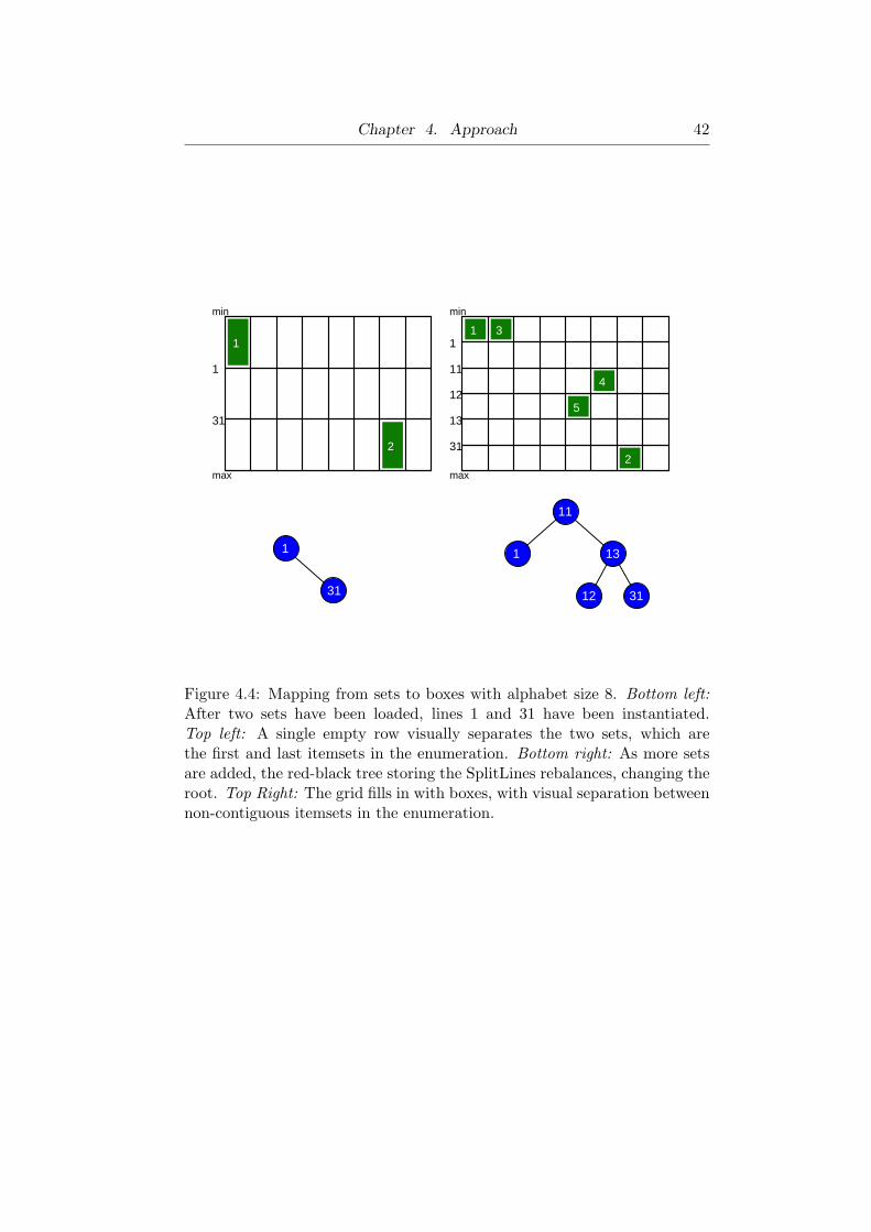
Construction of the SplitLine hierarchy can be further divided into two
subproblems: (a) when to instantiate a SplitLine and (b) how to update
necessary data structures to maintain the correct hierarchical structure. The
following example gives an overview of the mapping process on a database
with an alphabet size of eight items. As shown in Table 4.1, as sets are sent
to the visualizer, their enumeration index is computed and used to find the
row and column in the grid where boxes are drawn.
We instantiate a SplitLine when and only when (a) it has not been
Chapter 4. Approach 42
max
min
31
1
1
2
max
min
12
13
11
1
31
31
5
2
4
1
31
11
1 13
12 31
Figure 4.4: Mapping from sets to boxes with alphabet size 8. Bottom left:After two sets have been loaded, lines 1 and 31 have been instantiated.Top left: A single empty row visually separates the two sets, which arethe first and last itemsets in the enumeration. Bottom right: As more setsare added, the red-black tree storing the SplitLines rebalances, changing theroot. Top Right: The grid fills in with boxes, with visual separation betweennon-contiguous itemsets in the enumeration.

Chapter 4. Approach 43
No. Set Index Row Col Lines1 {a} 0 0 0 12 {a, b, c, d, e, f, g, h} 254 31 6 313 {b} 1 0 1 -4 {a, b, c, e} 93 11 5 11, 125 {a, b, d, h} 100 12 4 13
Table 4.1: As sets are sent to the visualizer, their enumeration index iscomputed and used to find the row and column in the grid where boxes aredrawn.
instantiated and (b) it serves as a boundary of at least one box.As shown in
Figure 4.4 top left, after the first two sets have been loaded, a single empty
row visually separates the two sets, which are the first and last itemsets in
the enumeration. The instantiation of the empty row is important in that it
servers as a visual cue to the user that the first two sets are not immediately
adjacent to each other. A corresponding SplitLine hierarchy is shown in
Figure 4.4 bottom left. Figure 4.4 top right shows the visualization after all
the sets have been loaded. As more sets are added, the red-black tree stores
the SplitLines, rebalances, and changes the root. The horizontal SplitLines
hierarchy would require 25 = 32 nodes if it were statically allocated, but
only 5 are needed when using dynamic allocation.
We need to insert a node in the corresponding red-black tree once we
have decided to create a SplitLine. Before we insert the node into the red-
black tree, we must calculate the default relative split position of each line,
which is used to set or reset its initial absolute position so that the lines
look uniformly distributed. If the number of SplitLines were a power of 2,
then we could simply set each one to the split position of 0.5. When the
binary tree is not perfectly balanced, then the correct value for a SplitLine
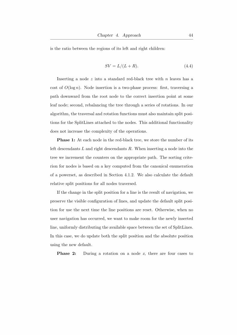
Chapter 4. Approach 44
is the ratio between the regions of its left and right children:
SV = L/(L + R). (4.4)
Inserting a node z into a standard red-black tree with n leaves has a
cost of O(log n). Node insertion is a two-phase process: first, traversing a
path downward from the root node to the correct insertion point at some
leaf node; second, rebalancing the tree through a series of rotations. In our
algorithm, the traversal and rotation functions must also maintain split posi-
tions for the SplitLines attached to the nodes. This additional functionality
does not increase the complexity of the operations.
Phase 1: At each node in the red-black tree, we store the number of its
left descendants L and right descendants R. When inserting a node into the
tree we increment the counters on the appropriate path. The sorting crite-
rion for nodes is based on a key computed from the canonical enumeration
of a powerset, as described in Section 4.1.2. We also calculate the default
relative split positions for all nodes traversed.
If the change in the split position for a line is the result of navigation, we
preserve the visible configuration of lines, and update the default split posi-
tion for use the next time the line positions are reset. Otherwise, when no
user navigation has occurred, we want to make room for the newly inserted
line, uniformly distributing the available space between the set of SplitLines.
In this case, we do update both the split position and the absolute position
using the new default.
Phase 2: During a rotation on a node x, there are four cases to
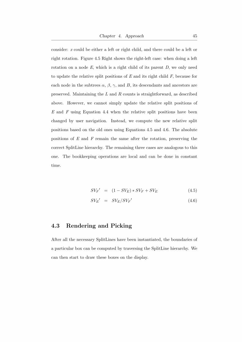
Chapter 4. Approach 45
consider: x could be either a left or right child, and there could be a left or
right rotation. Figure 4.5 Right shows the right-left case: when doing a left
rotation on a node E, which is a right child of its parent D, we only need
to update the relative split positions of E and its right child F, because for
each node in the subtrees α, β, γ, and B, its descendants and ancestors are
preserved. Maintaining the L and R counts is straightforward, as described
above. However, we cannot simply update the relative split positions of
E and F using Equation 4.4 when the relative split positions have been
changed by user navigation. Instead, we compute the new relative split
positions based on the old ones using Equations 4.5 and 4.6. The absolute
positions of E and F remain the same after the rotation, preserving the
correct SplitLine hierarchy. The remaining three cases are analogous to this
one. The bookkeeping operations are local and can be done in constant
time.
SVF′ = (1− SVE) ∗ SVF + SVE (4.5)
SVE′ = SVE/SVF
′ (4.6)
4.3 Rendering and Picking
After all the necessary SplitLines have been instantiated, the boundaries of
a particular box can be computed by traversing the SplitLine hierarchy. We
can then start to draw these boxes on the display.
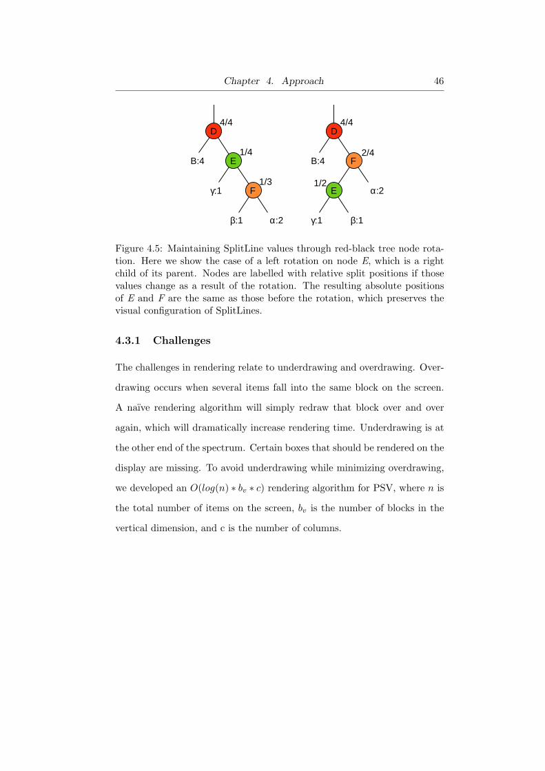
Chapter 4. Approach 46
D4/4
D4/4
E1/4
Β:4
γ:1
F2/4
Β:4
γ:1
F1/3
α:2β:1
E1/2
α:2
β:1
Figure 4.5: Maintaining SplitLine values through red-black tree node rota-tion. Here we show the case of a left rotation on node E, which is a rightchild of its parent. Nodes are labelled with relative split positions if thosevalues change as a result of the rotation. The resulting absolute positionsof E and F are the same as those before the rotation, which preserves thevisual configuration of SplitLines.
4.3.1 Challenges
The challenges in rendering relate to underdrawing and overdrawing. Over-
drawing occurs when several items fall into the same block on the screen.
A naıve rendering algorithm will simply redraw that block over and over
again, which will dramatically increase rendering time. Underdrawing is at
the other end of the spectrum. Certain boxes that should be rendered on the
display are missing. To avoid underdrawing while minimizing overdrawing,
we developed an O(log(n) ∗ bv ∗ c) rendering algorithm for PSV, where n is
the total number of items on the screen, bv is the number of blocks in the
vertical dimension, and c is the number of columns.
Chapter 4. Approach 47
4.3.2 Our Approach
Rendering
Rendering in PSV strictly follows the rendering pipeline described in
PRISAD [27]. The rendering process consists of three steps: partitioning,
seeding, and drawing. Partitioning is a discretization process that maps the
infinite-precision drawing of rectangular boxes to the desired block level. In
other words, we divide the world space into small regions of equal size, where
the number of regions is determined by the number of pixels available on the
display and the size of the on-screen blocks. If a particular region contains
only one set, we simply draw a box on the screen to represent the set. When
a region contains more than one set, which is the most common case, we need
to use other visual channels to encode aggregate information in addition to
drawing a box on the display. In our current implementation, the brightness
of a box is proportional to the number of sets in the region. Since SplitLines
also serve as the boundary of boxes, the discretization process in PSV is
done by dividing them into small regions. When the discretization process
is finished, we enqueue all the boxes that need to be rendered. Finally, we
traverse the rendering queue to render the boxes one at a time.
We maintain a red-black tree, NodeTree, for each column. The item set
that is mapped to a column will be attached to a node in the corresponding
red-black tree, where the index of the node is the row number of that item
set.
The NodeTree provides both a linear ordering and a hierarchical or-
ganization of the item sets (as shown in Figure 4.6), which is similar to
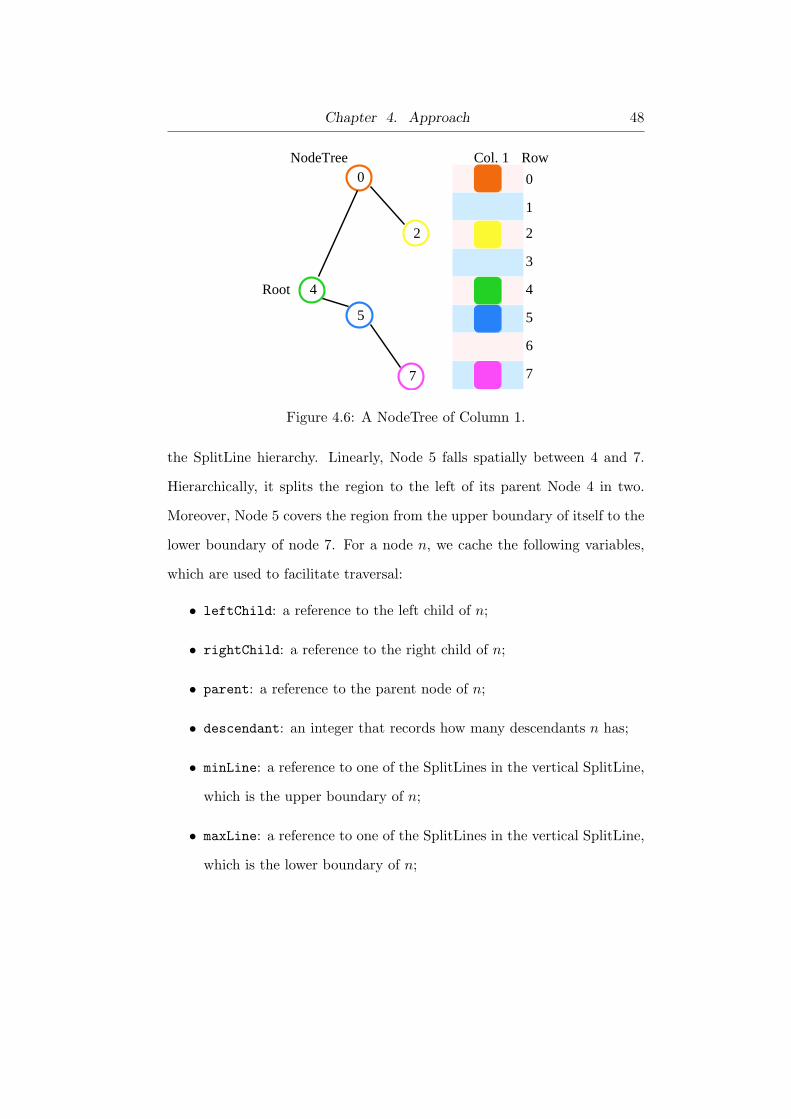
Chapter 4. Approach 48
1
2
3
4
5
6
7
0
RowCol. 1NodeTree
Root 4
7
2
5
0
Figure 4.6: A NodeTree of Column 1.
the SplitLine hierarchy. Linearly, Node 5 falls spatially between 4 and 7.
Hierarchically, it splits the region to the left of its parent Node 4 in two.
Moreover, Node 5 covers the region from the upper boundary of itself to the
lower boundary of node 7. For a node n, we cache the following variables,
which are used to facilitate traversal:
• leftChild: a reference to the left child of n;
• rightChild: a reference to the right child of n;
• parent: a reference to the parent node of n;
• descendant: an integer that records how many descendants n has;
• minLine: a reference to one of the SplitLines in the vertical SplitLine,
which is the upper boundary of n;
• maxLine: a reference to one of the SplitLines in the vertical SplitLine,
which is the lower boundary of n;

Chapter 4. Approach 49
• aggregate: a Boolean value that indicates whether n represents more
than one box;
• aggregateNumber: an integer that records how many boxes n repre-
sents; and
• fixed: a Boolean value that indicates whether n should be drawn in
a fixed size or in its actual size.
In addition, we compute the following variables on the fly, using standard
tree-traversal algorithms:
• nodeRange: the region that is split by node n. As shown in Figure 4.6,
the nodeRange of node 5 runs from the upper boundary of node 4 to
the lower boundary of node 7; and
• nodeCoverage: the region that is covered by node n. As shown in
Figure 4.6, nodeCoverage of node 5 runs from the upper boundary of
node 5 to the lower boundary of node 7.
We perform a recursive binary subdivision on the NodeTree hierarchy.
Recursion is dependent on either the world-space criterion that the Node
has no children, or the image-space criterion that the Node’s range currently
subtends less than one block.
Figure 4.7 illustrates the three cases that determine whether the recur-
sion should terminate or continue. In case 1, for Nodes 4 and 0, the node
coverage is larger than one block size and has child nodes, so we descend
to both children. Node 5 shows case 2, since its coverage spans less than
one block. We stop the recursion and draw a box to represent Node 5 and

Chapter 4. Approach 50
1
2
3
4
5
6
7
0
RowCol. 1NodeTree
7
2
0
Root 45
Case 1
Case 1
Case 3
Case 2
Figure 4.7: The three cases used to determine how to descend the NodeTreehierarchy.
its descendant (Node 7). Finally, Node 2 is a leaf node in the NodeTree
hierarchy, and recursion stops.
Algorithm 1 shows the pseudocode of the enqueuing function,
enqueueRecurse(Node node). Line 1 to line 6 ensure that node does not
overlap with any boxes that are already in the rendering queue. If node over-
laps with a box b in the rendering queue, b will be updated to an “aggregate”
box and rendered accordingly. Line 8 to line 16 flag node.fixed variable if
its actual size is smaller than one block. Line 18 evaluates if node is a leaf
node and line 20 decides whether node’s coverage is less than one block.
The number of recursions is bounded by the number of boxes in the vertical
direction, bv. Each of the recursions requires traversing the SplitLine data
structure with a complexity of O(log(n)), where n is the total number of
item sets. Therefore, the overall complexity of the enqueuing function is
O(log(n) ∗ bv).

Chapter 4. Approach 51
Algorithm 1 Enqueuing Function: enqueueRecurse(Node node)1: if node.minLine−node.nodeRange.minLine<unitBlockLength then2: node.nodeRange.minNode.aggregate = true3: node.nodeRange.minNode.aggregateNumber++4: else if node.nodeRange.max−node.minLine<unitBlockLength then5: node.nodeRange.maxNode.aggregate = true6: node.nodeRange.maxNode.aggregateNumber++7: else8: if node.maxLine.getPosition()−node.minLine.getPosition()
≥unitBlockLength then9: node.fixed=false
10: node.aggregate=false11: enqueue node;12: else13: node.fixed=true14: node.aggregate=false15: enqueue node;16: end if17: end if18: if node is a leaf node then19: return20: else if node.nodeCoverage<unitBlockLength then21: return22: else if node.leftChild6=null then23: renderRecurse(node.leftChild)24: else if node.rightChild6=null then25: renderRecurse(node.rightChild26: end if
Chapter 4. Approach 52
In the second phase of the rendering pipeline, we traverse the render-
ing queue and render as many boxes as we can in a given time slot. This
technique is called progressive rendering. Progressive rendering is a tech-
nique that renders the entire scene in a prioritized fashion. It always renders
the most important part of the scene first and then fills in the details. If the
time that is allocated for rendering this scene is used up, progressive render-
ing just stops rendering the current scene and immediately starts drawing
the next scene, which makes the system very responsive. In PSV, we start
the rendering process from the columns that are within the user’s navigation
box, because user navigation in this area implies that it is of great interest
to the user.
Picking
Picking is the process of identifying which object was rendered at a particular
(x, y) pixel location. Picking also requires traversing both the NodeTree
and SplitLine hierarchies. Picking is done in two steps. The first step is to
traverse the horizontal SplitTree to find the correct column. In the second
step, we retrieve the NodeTree from the correct column and do a traversal,
which is similar to the binary search, to find the correct node, if one exists.
Algorithm 2 shows the pseudocode of the picking function. The input of
this function is the root node of the selected column’s NodeTree.
Sometimes, the actual size of a box could be too tiny to be easily picked
by the user. A well-selected fuzzConstant is used to ensure that every box
that is visible on screen is pickable by allowing an offset of a few pixels.
The complexity of this function is O(log(n)), where n is the total number
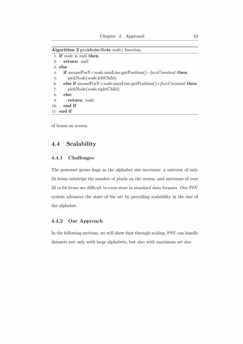
Chapter 4. Approach 53
Algorithm 2 pickNode(Node node) function.1: if node is null then2: return null3: else4: if mousePosY<node.minLine.getPosition()−fuzzConstant then5: pickNode(node.leftChild)6: else if mousePosY>node.maxLine.getPosition()+fuzzConstant then7: pickNode(node.rightChild)8: else9: return node
10: end if11: end if
of boxes on screen.
4.4 Scalability
4.4.1 Challenges
The powerset grows huge as the alphabet size increases: a universe of only
24 items outstrips the number of pixels on the screen, and universes of over
32 or 64 items are difficult to even store in standard data formats. Our PSV
system advances the state of the art by providing scalability in the size of
the alphabet.
4.4.2 Our Approach
In the following sections, we will show that through scaling, PSV can handle
datasets not only with large alphabets, but also with maximum set size.

Chapter 4. Approach 54
Handling Large Alphabets
When the alphabet size A is large, the powerset size P is a huge number:
2A. Dynamic allocation of the SplitLine hierarchy, as discussed above, is
necessary but not sufficient. The indices in the power enumeration do not
fit into an integer or a long integer when the alphabet size is greater than
31 or 63, whereas we support alphabets of over 40,000 items. The naıve ap-
proach would be to simply switch data structures from integer to bignum
everywhere that indices are used in the SplitLine hierarchy. However, com-
putations using bignums are far more expensive than those using integers
or longs, and storing them imposes a heavy memory footprint, so we would
like to minimize their use. In contrast, the visualizer must store all N sets
actually shown in main memory, so our algorithms are optimized for the
case where N << P . In the current implementation, N is limited to the
range of 1.5 to 7 million sets, a number far smaller than the 2 trillion limit of
integer data storage. Operations that use the number of shown sets N can
be done much more efficiently, as opposed to those that use the alphabet
size A or the powerset size P .
Our spatial layout does fundamentally depend on the powerset size P ,
so we cannot completely eliminate bignums. The key insight is that we only
need to use these high-precision values when adding SplitLines from the
hierarchy as sets are added to the scene. Specifically, we use bignums in two
computations: finding the enumeration index as described by Equation 4.2,
and then when dividing that index by the fixed width of the grid to get a
bignum row index. The row index does need to be stored: as illustrated

Chapter 4. Approach 55
in Figure 4.4, a full-precision SplitLine row index may be necessary when
resolving the spatial relationship between the box in question and boxes
that are added or deleted later. By storing this row index as a bignum, we
support lazy evaluation and avoid unnecessary computation. Although the
computation of the enumeration index requires bignums, we do not need to
incur the memory overhead of storing it, so we throw it away after its use
in computing the row index.
Our rendering and navigation routines remain fast because we do not
need to use bignums when traversing the SplitLine hierarchy. Although the
bignum row indices must be stored at each node of the hierarchy, we can
traverse the tree without them by maintaining pointers or object references
in the node data structure linking it to its children and parent.
Extending the Maximum Set Size
Often dataset semantics dictate that the maximum set size is much smaller
than the alphabet size. For example, it is essentially impossible to buy
every item in a grocery store in one shopping trip or to take the thousands
of courses offered at a university during the same term. Figure 5.3 shows
that a university enrollment dataset with alphabet 4616 has a maximum set
size of 13, and the market basket data in Figure 5.6 has a maximum set
size of 115 out of the 1700 items in the alphabet. In contrast, although the
particular software engineering dataset shown in Figure 6.1 has a maximum
set size of 48 files checked in together during a bug fix out of 42,028 files in the
alphabet, the domain semantics could allow a maximum set commensurate
with the entire alphabet. For instance, if the copyright notice on top of

Chapter 4. Approach 56
each file needs changing, every file in the repository would be touched. An
important property of our algorithm is that there is no hardwired prior limit
on the maximum set size; we can accommodate a maximum set size up to
the cardinality of the alphabet itself.
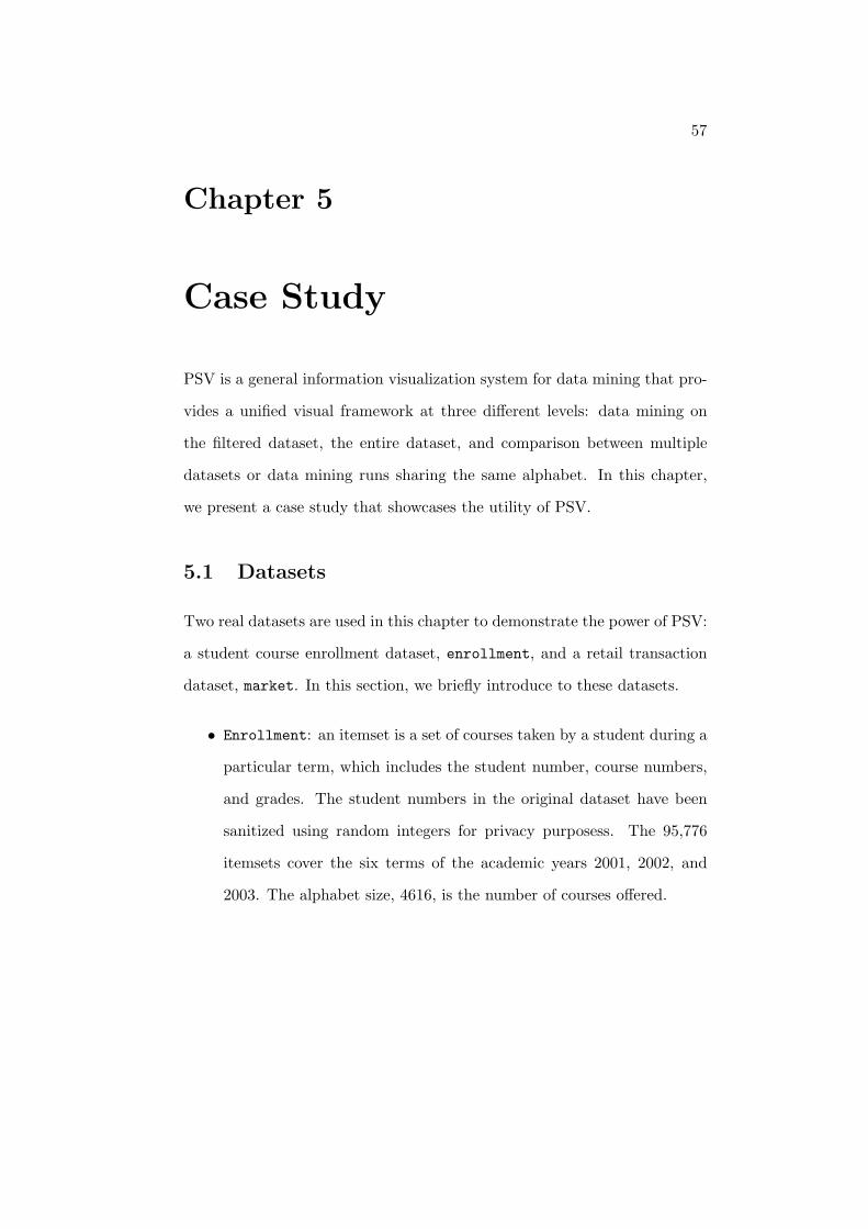
57
Chapter 5
Case Study
PSV is a general information visualization system for data mining that pro-
vides a unified visual framework at three different levels: data mining on
the filtered dataset, the entire dataset, and comparison between multiple
datasets or data mining runs sharing the same alphabet. In this chapter,
we present a case study that showcases the utility of PSV.
5.1 Datasets
Two real datasets are used in this chapter to demonstrate the power of PSV:
a student course enrollment dataset, enrollment, and a retail transaction
dataset, market. In this section, we briefly introduce to these datasets.
• Enrollment: an itemset is a set of courses taken by a student during a
particular term, which includes the student number, course numbers,
and grades. The student numbers in the original dataset have been
sanitized using random integers for privacy purposess. The 95,776
itemsets cover the six terms of the academic years 2001, 2002, and
2003. The alphabet size, 4616, is the number of courses offered.
Chapter 5. Case Study 58
• Market: a record in this dataset is a set of items that are bought
together by a particular customer during a single visit to a store. This
dataset was downloaded from UCI Machine Learning Repository 1 and
had been sanitized. This dataset contains 300,000 transactions and has
1657 items.
5.2 Enrollment Dataset
5.2.1 Frequent-Set Mining
We chose dynamic, constrained frequent-set mining as a concrete case study.
Frequent-set mining is the process of identifying groupings of co-appearing
objects in a dataset, whose frequencies exceed a user-specified threshold.
The appeal of constrained frequent-set mining is well known [23, 8, 20]. One
key problem that has not been addressed in previous work is how to support
users in choosing and changing constraint thresholds and parameters. This
unsolved problem makes dynamic constrained frequent-set mining a perfect
case study for showcasing the power of our visualization system.
At the beginning of the task, the analyst specifies a set of constraints and
a frequency threshold. Sets that both satisfy the constraints and pass the
frequency threshold will be returned to PSV. Finally, PSV will render the
sets returned by the mining engine on the display to give analysts immediate
visual feedback of the mining result.
PSV is able to communicate with the mining engine using a simple text
protocol, which includes constraint settings, pause, and play. Users1http://www.ics.uci.edu/˜mlearn/MLRepository.html

Chapter 5. Case Study 59
can pause the mining engine to tighten or relax the parameter settings based
on the partial result.
In the current implementation of PSV, users are able to specify the
following types of constraints for interactive constrained frequent-set mining:
(a) aggregation constraints of the form “agg(resultSet.A) θ const”,
where (i) agg is an aggregate operator (e.g., MAX, MIN, MEAN,
MEDIUM, SUM), (ii) A is an auxiliary attribute (e.g., class size, class
average for the student record database), (iii) θ is a comparison op-
erator (e.g., =, >, <,≥,≤), and (iv) const is an integer constant. For
example, the constraint “MAX(resultSet. classSize) < 100” finds all
the sets of courses having a maximum class size of less than 100.
(b) the frequency constraint “frequency(resultSet) ≥ threshold”, which
finds all the sets whose occurrences in the dataset meet or exceed the
user-specified threshold. For example, the constraint
“frequency(resultSet) ≥ 0.001” finds all the sets that appear in at least
0.1% of the transactions in the dataset.
(c) containment constraints of the form “resultSet contains ConstSet”,
where ConstSet is a set of constants. Here, this type of constraints
finds all the sets that contain any of the constants in ConstSet. For
example, the constraint “resultSet contains {CPSC124, CPSC126}”finds all the sets that contain the course CPSC124 or CPSC126.
Constraints are processed at different locations within PSV: some can
be handled by both the visualizer and the miner, while others are only
Chapter 5. Case Study 60
processed by the miner or only processed by the visualizer. Frequency con-
straints are computationally intensive, and are thus “pushed inside” to the
miner, in order to provide as much pruning as possible. The miner can
handle a combination of frequency and aggregation constraints. Sets that
satisfy these miner constraints are sent to the visualizer for display. Speci-
fying constraints for the miner is also a way of filtering datasets larger than
the current 7-million itemset capacity of the visualizer, which maintains all
loaded itemsets in main memory to support fluid realtime exploration.
The visualizer supports aggregation and containment constraints by vi-
sually highlighting the matching sets from among those it has loaded. It
can handle multiple simultaneous constraints, colouring each with a differ-
ent colour.
The visualizer supports immediate exploration of multiple simple con-
straints but has the limited capacity of 7 million itemsets, whereas the miner
can handle very large datasets and more sophisticated constraints but re-
quires a longer period of time for computation.
5.2.2 Usage Scenarios
We present four scenarios of PSV features being used during a data-mining
task. These scenarios are built around the real course enrollment database,
where an itemset is the set of courses taken by a student during a particular
term. The 95,776 items cover the six terms of the academic years 2001,
2002, and 2003. The alphabet size, 4616, is the total number of courses
offered. Our example user is an undergraduate course coordinator interested
in finding sets of courses that are frequently taken together, so that she can

Chapter 5. Case Study 61
minimize conflicts when scheduling courses for the following year.
Scenario 1: The coordinator first considers medium-sized courses, and
decides to start with an enrollment threshold of 100. Her first constrained
frequent-set query is frequency ≥ 0.005 and max(courseSize) ≤ 100. The
result of the query shows all possible sets of courses such that the set ap-
pears in at least 0.5% of all student registration records and that have a
maximum class size of less than 100. She watches the visualizer display as
it dynamically updates to show the progress of the miner, and notices from
the sparseness of the display that her initial parameter setting might not
be appropriate. Figure 5.1 shows the constrained frequent sets computed so
far when she pauses the computation after 10% of the itemsets have been
processed. The sets are shown as a distribution of small boxes ordered by
cardinality, from singleton sets at the top to 5-sets on the bottom. (Hereafter
we use the convention of k-sets to denote sets of size k.) Each cardinality
has a different background colour, and within each cardinality the sets are
enumerated in lexicographic order, as discussed in Section 4.1. The coordi-
nator loosens the frequency constraint to .001, and tightens the enrollment
parameter to 80 or fewer students before resuming the computation. Fig-
ure 5.2 shows the final result with the new constraints. After all ninety-six
thousand itemsets have been processed by the miner, the largest constrained
frequent itemset is a 9-set, whereas the largest set in the partial result in
Figure 5.1 is a 5-set.
Scenario 2: The coordinator now returns to the question of what course
size would represent her intuitive idea of “medium”. Instead of filtering the
itemsets with the miner, she loads in the entire database in pass-through

Chapter 5. Case Study 62
Figure 5.1: Scenario 1 for data mining with PSV. The user pauses after 10%of the itemsets are processed to loosen the frequency constraint and tightenthe other parameters.
Figure 5.2: Scenario 1 for data mining with PSV. After the user’s refinement,the view is considerably denser, showing higher cardinality sets, after all theitemsets are processed.
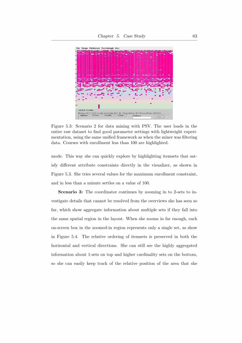
Chapter 5. Case Study 63
Figure 5.3: Scenario 2 for data mining with PSV. The user loads in theentire raw dataset to find good parameter settings with lightweight experi-mentation, using the same unified framework as when the miner was filteringdata. Courses with enrollment less than 100 are highlighted.
mode. This way she can quickly explore by highlighting itemsets that sat-
isfy different attribute constraints directly in the visualizer, as shown in
Figure 5.3. She tries several values for the maximum enrollment constraint,
and in less than a minute settles on a value of 100.
Scenario 3: The coordinator continues by zooming in to 2-sets to in-
vestigate details that cannot be resolved from the overviews she has seen so
far, which show aggregate information about multiple sets if they fall into
the same spatial region in the layout. When she zooms in far enough, each
on-screen box in the zoomed-in region represents only a single set, as show
in Figure 5.4. The relative ordering of itemsets is preserved in both the
horizontal and vertical directions. She can still see the highly aggregated
information about 1-sets on top and higher cardinality sets on the bottom,
so she can easily keep track of the relative position of the area that she
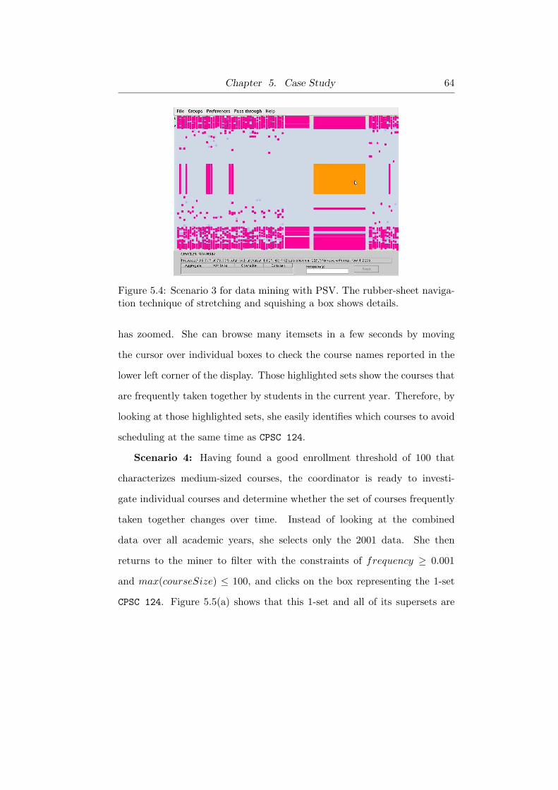
Chapter 5. Case Study 64
Figure 5.4: Scenario 3 for data mining with PSV. The rubber-sheet naviga-tion technique of stretching and squishing a box shows details.
has zoomed. She can browse many itemsets in a few seconds by moving
the cursor over individual boxes to check the course names reported in the
lower left corner of the display. Those highlighted sets show the courses that
are frequently taken together by students in the current year. Therefore, by
looking at those highlighted sets, she easily identifies which courses to avoid
scheduling at the same time as CPSC 124.
Scenario 4: Having found a good enrollment threshold of 100 that
characterizes medium-sized courses, the coordinator is ready to investi-
gate individual courses and determine whether the set of courses frequently
taken together changes over time. Instead of looking at the combined
data over all academic years, she selects only the 2001 data. She then
returns to the miner to filter with the constraints of frequency ≥ 0.001
and max(courseSize) ≤ 100, and clicks on the box representing the 1-set
CPSC 124. Figure 5.5(a) shows that this 1-set and all of its supersets are

Chapter 5. Case Study 65
(a)
Yea
r2001
(b)
Yea
r2003
Fig
ure
5.5:
(a):
CPSC124
and
its
supe
rset
sar
ehi
ghlig
hted
for
the
acad
emic
year
2001
.(b
):th
esa
me
cour
sean
dit
ssu
pers
ets
are
high
light
edfo
rth
eac
adem
icye
ar20
03.
Chapter 5. Case Study 66
highlighted. In other words, she can see the upward closure property of the
containment relation. Using lattice terminology, the highlighted elements
form a lower semi-lattice with CPSC 124 as the bottom element, and satisfy
all the specified constraints. The courses contained in these highlighted sets
are the ones to avoid scheduling simultaneously with CPSC 124. She then
starts up a second copy of PSV with the same configuration on the academic
year 2003 data, as shown in Figure 5.5(b). With the 2001 and 2003 displays
side by side, she can quickly spot differences and mouseover those boxes to
find the names of courses that became less popular to take with CPSC 124.
5.3 Market Dataset
Figure 5.6 shows the result of the Market dataset. The numbers on the
left side of the window indicate the size of the sets or the number of items
bought together by a customer during a single shopping trip. It is easy to
determine that the upper part of the window is much denser than the lower
part, which means that customers are less likely to buy many items at a
time. After a close look at the final visualization, we confirm that most
of the transactions consist of fewer than six items. Interestingly, the top
part of the region for singleton sets is denser than the lower part, which
implies that the products listed in the head part of the alphabet are more
popular than those in the tail part. Unfortunately, we are unable to identify
those products to conduct further analysis, since the Market dataset has no
attribute.
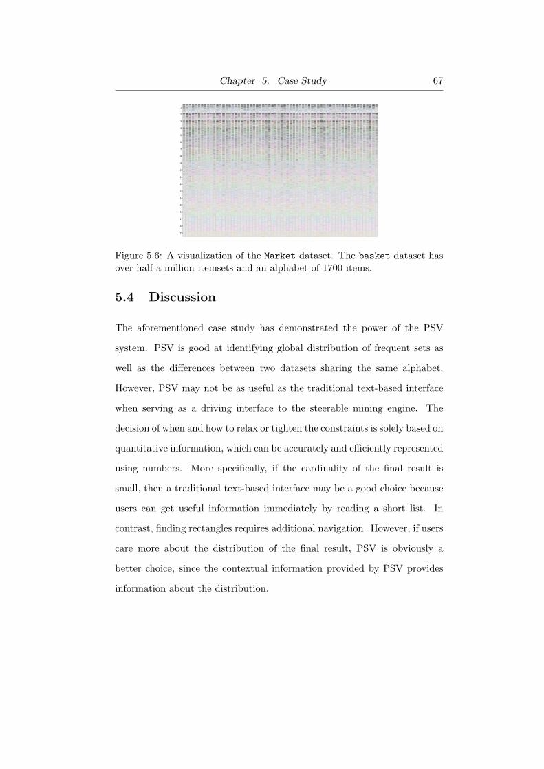
Chapter 5. Case Study 67
1
2
3
4
5
6
7
8
9
10
11
12
13
14
15
16
17
18
19
Figure 5.6: A visualization of the Market dataset. The basket dataset hasover half a million itemsets and an alphabet of 1700 items.
5.4 Discussion
The aforementioned case study has demonstrated the power of the PSV
system. PSV is good at identifying global distribution of frequent sets as
well as the differences between two datasets sharing the same alphabet.
However, PSV may not be as useful as the traditional text-based interface
when serving as a driving interface to the steerable mining engine. The
decision of when and how to relax or tighten the constraints is solely based on
quantitative information, which can be accurately and efficiently represented
using numbers. More specifically, if the cardinality of the final result is
small, then a traditional text-based interface may be a good choice because
users can get useful information immediately by reading a short list. In
contrast, finding rectangles requires additional navigation. However, if users
care more about the distribution of the final result, PSV is obviously a
better choice, since the contextual information provided by PSV provides
information about the distribution.
Chapter 5. Case Study 68
In the student enrollment example, given a course, a typical user might
be interested in only the top 10 courses that are taken together with the
course of interest in a specified period. The result can be shown to the user
simply using a short list. The additional contextual information does not
facilitate the user’s job. On the contrary, unnecessary navigation resulting
from discovering the detailed information requires extra effort.
We tried to showcase the utility of PSV in other domains, such as soft-
ware engineering and algorithms. However, based on our research and in-
terviews with several domain experts, it was difficult to find examples that
required the full power of PSV. PSV has the ability to allow users to explore
in a huge search space, but most domain-specific problems do not require
showing or searching the result in the context of the entire search space.
69
Chapter 6
Performance
In this chapter, we discuss the performance of the PSV system with both
real and synthetic datasets. We document that PSV can scale to datasets
of up to 7 million itemsets and alphabet sizes of over 40,000 items, while
maintaining interactive rendering speeds of under 60 milliseconds per frame.
6.1 Datasets
6.1.1 Mozilla Dataset
We use the Mozilla dataset to show that PSV can accommodate datasets
with alphabet sizes of over 40,000 items. The Mozilla dataset is a software
engineering dataset from the open-source Mozilla project 1. It was down-
loaded from the Bugzilla 2 bug database and was compiled by Anne Ying.
An itemset is a set of files that have been checked in together after a re-
vision task is done. Each itemset contains the file names and their version
numbers. There are 33,407 check-in records and 42,028 files in the Mozilla
dataset. The final visualization is shown in Figure 6.1.1http://www.mozilla.org2http://www.bugzilla.org/

Chapter 6. Performance 70
Figure 6.1: The Mozilla dataset has 42,028 itemsets and an alphabet of42,028 items.
6.1.2 Synthetic Datasets
To showcase the memory usage and rendering performance of PSV, we gener-
ate two synthetic datasets, sparse and dense. The dense synthetic dataset
is the extreme case of the densest possible distribution: items in the dataset
are the first 10 million items in the full powerset generated from a dataset
with an alphabet of 10,000 items. The sparse synthetic dataset has a dis-
tribution density roughly similar to the market dataset, and uses the same
alphabet.
6.1.3 Datasets Summary
Table 6.1 summarizes the datasets introduced in the previous sections.
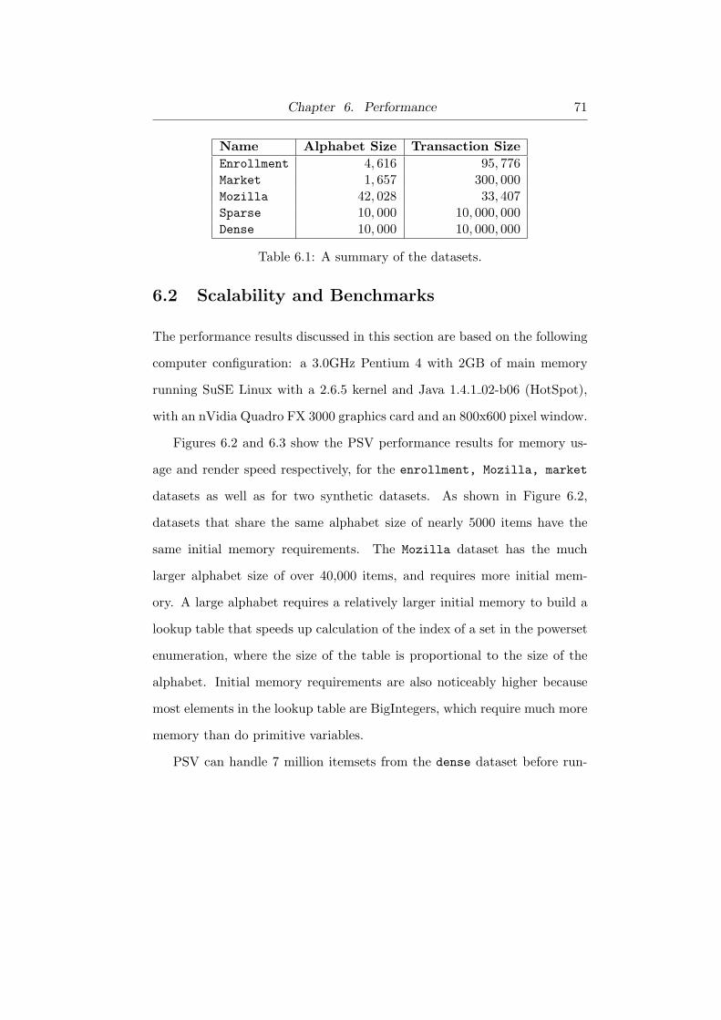
Chapter 6. Performance 71
Name Alphabet Size Transaction SizeEnrollment 4, 616 95, 776Market 1, 657 300, 000Mozilla 42, 028 33, 407Sparse 10, 000 10, 000, 000Dense 10, 000 10, 000, 000
Table 6.1: A summary of the datasets.
6.2 Scalability and Benchmarks
The performance results discussed in this section are based on the following
computer configuration: a 3.0GHz Pentium 4 with 2GB of main memory
running SuSE Linux with a 2.6.5 kernel and Java 1.4.1 02-b06 (HotSpot),
with an nVidia Quadro FX 3000 graphics card and an 800x600 pixel window.
Figures 6.2 and 6.3 show the PSV performance results for memory us-
age and render speed respectively, for the enrollment, Mozilla, market
datasets as well as for two synthetic datasets. As shown in Figure 6.2,
datasets that share the same alphabet size of nearly 5000 items have the
same initial memory requirements. The Mozilla dataset has the much
larger alphabet size of over 40,000 items, and requires more initial mem-
ory. A large alphabet requires a relatively larger initial memory to build a
lookup table that speeds up calculation of the index of a set in the powerset
enumeration, where the size of the table is proportional to the size of the
alphabet. Initial memory requirements are also noticeably higher because
most elements in the lookup table are BigIntegers, which require much more
memory than do primitive variables.
PSV can handle 7 million itemsets from the dense dataset before run-

Chapter 6. Performance 72
ning out of memory, which limits supportable dataset size. The limits of
PSV depend on the distribution of the dataset within the powerset. Sparser
datasets require the instantiation of more SplitLines than do dense ones,
resulting in less total capacity in the visualizer. The sparse dataset rep-
resents a typical use case. PSV can handle over 1.5 million itemsets from
this dataset family before its memory footprint outstrips the maximum Java
heap size of 1.7GB. We reiterate that when using the miner as a filter, PSV
as a client-server system can handle much larger datasets than the limits of
the visualizer.
Figure 6.3 top shows that the rendering time is near-constant after a
threshold dataset size has been reached. This constant time is very small:
60 milliseconds per scene, allowing over 15 frames per second even in the
worst-case scenario. Render time also depends linearly on the horizontal
width of the grid.
We are also interested in the performance when part or all of the on-
screen sets are highlighted, since grouping and highlighting are the two most
commonly used features in PSV. In PSV, a set can belong to multiple groups
at the same time. The colour of the set is determined by the colour of the
group having the highest priority. However, we do not determine colour on
the fly, since the cost of querying and of changing OpenGL context may be
very high. In the current implementation, when a set belongs to n groups
we simply redraw the set n times in n different depths based on the group
priorities. We rely on the Z-buffer to assign the correct colour to the set.
Based on the results of our empirical experiments, the cost of redrawing a
set multiple times is much less than that of determining the colour on the
Chapter 6. Performance 73
fly, considering that a set is not likely to belong to more than three groups
at the same time. In the worst-case scenario, when each of the n groups
contains all sets, rendering time is n times that of the normal case where no
sets are highlighted.
The main challenge PSV presented with us was to accommodate large
alphabet and maximum set sizes, a difficult goal given the exponential nature
of the powerset used for spatial layout. We have done so, showing examples
of PSV in use on alphabets ranging from 4,000 to over 40,000 items. Larger
alphabets require more bits in the bignums used in enumeration, affecting
both the speed and memory usage of PSV.
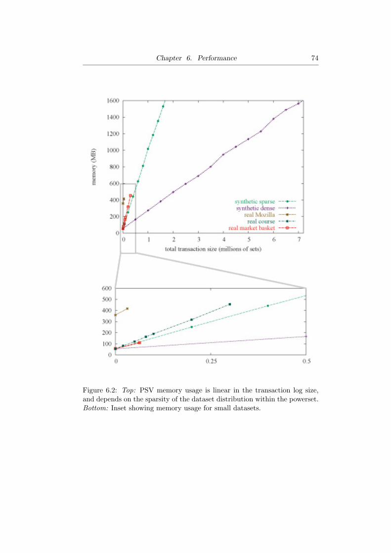
Chapter 6. Performance 74
Figure 6.2: Top: PSV memory usage is linear in the transaction log size,and depends on the sparsity of the dataset distribution within the powerset.Bottom: Inset showing memory usage for small datasets.

Chapter 6. Performance 75
Figure 6.3: Top: PSV rendering time is under 60 milliseconds per frame,near-constant after passing a threshold, and linear in the width of the grid.Bottom: Inset showing render times for small datasets.
76
Chapter 7
Conclusion and Future Work
In this thesis, we have reported the design and implementation of the PSV
visualization system for lattice-based mining of powersets. PSV provides a
unified visual framework at three different levels: data mining on the filtered
dataset and the entire dataset, and comparison between multiple datasets
sharing the same alphabet. PSV is also connected to a dynamic frequent-
set mining server, showcasing how this visualization approach helps users
exploit the power of steerability.
The key technical challenge for PSV is the size of the alphabet. We de-
velop a fast scheme for computing the enumeration position of a given m-set
in O(m) time, devise a dynamic data structure for managing SplitLines, and
handle bignums carefully to avoid inefficiencies. We conduct case studies of
the PSV system with real datasets. We also use synthetic datasets to ex-
pose the limits of the current implementation of the PSV system. Empirical
evaluation shows that the current version is capable of handling an alphabet
size over 40,000 items and a transaction dataset exceeding 7 million trans-
actions. Maintaining high frame rates is critical to the success of interactive
visual mining, and our framework successfully keeps the time required to
render the entire visible scene under one tenth of a second.
Chapter 7. Conclusion and Future Work 77
There are several limitations of our work. As the main motivation of
PSV, frequent-set mining is not the perfect example for showcasing its power,
since showing the final result in the context of the entire search space is not
a key factor in achieving the tasks introduced in Chapter 5. This leads to a
central question concerning PSV: when do we require distribution informa-
tion? It is not easy to find compelling examples in other domains, however,
we are still in search of clear tasks and/or datasets with more attributes,
where the full power of PSV will be utilized.
There are several directions we would like to pursue in future work.
First, we would like to characterize the effectiveness of different enumera-
tion orderings in helping users find visual patterns that convey important
information about the dataset. We would like to offer users flexibility in
ordering the powerset. Specifically, people may attach different weights to
all or some of the items. The second-tier ordering of the powersets will be
based on the weight of the item, to ensure that itemsets containing “heav-
ier” or more important items will appear before “lighter” or less important
itemsets.
Second, we would like to juxtapose different datasets sharing the same
alphabet in a single window. In the current implementation, users need to
run two copies of PSV to compare two datasets that share the same alphabet;
they must switch back and force to compare the two visualizations. It would
be ideal to offer users the opportunity to view different datasets in a single
copy of PSV. We may also employ a brushing and linking technique, so that
users may easily identify the relationships among different datasets.
Finally, we would like to adapt the current version of PSV to support

Chapter 7. Conclusion and Future Work 78
comparing different partial data-mining outcomes for other data-mining
tasks, including sequential-pattern mining [2], decision-tree construction [4,
12], and clustering [18]. Moreover, because finding frequent set is the first
step in identifying association rules, we would like to enable PSV to support
discovering association rules. We also would like to continue to explore the
possibility of applying PSV in other domains, such as software engineering
and algorithms.

79
Bibliography
[1] Rakesh Agrawal and Ramakrishnan Srikant. Fast algorithms for mining
association rules in large databases. In Proc. VLDB, pages 487–499,
1994.
[2] Rakesh Agrawal and Ramakrishnan Srikant. Mining sequential pat-
terns. In Proc. ICDE, pages 3–14, 1995.
[3] Christopher Ahlberg. Spotfire: an information exploration environ-
ment. SIGMOD Rec., 25(4):25–29, 1996.
[4] Mihael Ankerst, Christian Elsen, Martin Ester, and Hans-Peter Kriegel.
Visual classification: an interactive approach to decision tree construc-
tion. In Proc. KDD, pages 392–396, 1999.
[5] Dale Beermann, Tamara Munzner, and Greg Humphreys. Scalable,
robust visualization of large trees. In Proc. EuroVis, pages 37–44, 2005.
[6] Stefan Berchtold, H. V. Jagadish, and Kenneth A. Ross. Independence
diagrams: A technique for visual data mining. In Proc. KDD, pages
139–143, 1998.
[7] J. Bertin. Semiology of Graphics. University of Wisconsin Press, 1983.
Bibliography 80
[8] Cristian Bucile, Johannes Gehrke, Daniel Kifer, and Walker White.
Dualminer: A dual-pruning algorithm for itemsets with constraints.
Data Min. Knowl. Discov., 7(3):241–272, 2003.
[9] Thomas H. Cormen, Charles E. Leiserson, and Ronald L. Rivest. In-
troduction to Algorithms. MIT Press, 1990.
[10] W. J. Frawley, G. Piatetsky-Shapiro, and C. J. Matheus. Knowledge
discovery in databases - an overview. AI Magazine, 13:57–70, 1992.
[11] Jianchao Han and Nick Cercone. AViz: A visualization system for
discovering numeric association rules. In Proc. PAKKD, pages 269–
280, 2000.
[12] Jianchao Han and Nick Cercone. RuleViz: a model for visualizing
knowledge discovery process. In Proc. KDD, pages 244–253, 2000.
[13] Heike Hofmann, Arno P. J. M. Siebes, and Adalbert F. X. Wilhelm.
Visualizing association rules with interactive mosaic plots. In Proc.
KDD, pages 227–235, 2000.
[14] Tomonari Kamba, Shawn A. Elson, Terry Harpold, Tim Stamper, and
Piyawadee Sukaviriya. Using small screen space more efficiently. In
CHI ’96: Proceedings of the SIGCHI Conference on Human Factors in
Computing Systems, pages 383–390, New York, NY, USA, 1996. ACM
Press.
Bibliography 81
[15] Daniel A. Keim and Hans-Peter Kriegel. Visualization techniques for
mining large databases: A comparison. IEEE Trans. Knowledge and
Data Engineering, 8(6):923–938, 1996.
[16] Donald E. Knuth. personal communication, November 2004.
[17] Donald E. Knuth. The Art of Computer Programming, volume 4.
Addison-Wesley, 2005.
[18] Yehuda Koren and David Harel. A two-way visualization method for
clustered data. In Proc. KDD, pages 589–594, 2003.
[19] Jordan Lee. Powersetviewer: An interactive data mining application.
UBC CPSC533C 2004 course project final report.
[20] Carson Leung, Laks V.S. Lakshmanan, and Raymond T. Ng. Exploiting
succinct constraints using FP-trees. ACM Trans. Database Systems,
28:337–389, 2003.
[21] Tamara Munzner, Francois Guimbretiere, Serdar Tasiran, Li Zhang,
and Yunhong Zhou. TreeJuxtaposer: scalable tree comparison using
Focus+Context with guaranteed visibility. ACM Trans. Graph. (Proc.
SIGGRAPH), 22(3):453–462, 2003.
[22] Tamara Munzner, Raymond T. Ng, Qiang Kong, Jordan Lee, Janek
Klawe, Dragana Radulovic, and Carson K. Leung. Visual mining of
powersets with large alphabets. Technical Report TR-2005-25, Univer-
sity of British Columbia, 2005.
Bibliography 82
[23] Raymond T. Ng, Laks V. S. Lakshmanan, Jiawei Han, and Alex Pang.
Exploratory mining and pruning optimizations of constrained associa-
tions rules. In Proc. SIGMOD, pages 13–24, 1998.
[24] S.G. Parker and C.R. Johnson. SCIRun: A scientific programming
environment for computational steering. In Supercomputing, 1995.
[25] Ben Shneiderman. The eyes have it: A task by data type taxonomy for
information visualizations. In IEEE Visual Languages, pages 336–343,
1996.
[26] James Slack. A Partitioned Rendering Infrastructure for Stable Accor-
dion Navigation. Master’s thesis, University of British Columbia, May
2005.
[27] James Slack, Kristian Hildebrand, and Tamara Munzner. PRISAD: A
partitioned rendering infrastructure for scalable accordion drawing. In
Proc. InfoVis, pages 41–48, 2005.
[28] James Slack, Kristian Hildebrand, Tamara Munzner, and Katherine St.
John. SequenceJuxtaposer: Fluid navigation for large-scale sequence
comparison in context. In Proc. German Conference on Bioinformatics,
pages 37–42, 2004.
[29] Chris Stolte, Diane Tang, and Pat Hanrahan. Polaris: A system for
query, analysis, and visualization of multidimensional relational data-
bases. IEEE Trans. Vis. Comput. Graph., 8(1):52–65, 2002.

Bibliography 83
[30] Chris Stolte, Diane Tang, and Pat Hanrahan. Query, analysis, and
visualization of hierarchically structured data using Polaris. In Proc.
KDD, pages 112–122, 2002.
[31] Edward Tufte. Envisioning Information. Graphics Press, 1990.
[32] Colin Ware. Information Visualization: Perception for Design. Morgan
Kaufmann Publishers, 2000.
[33] Matt Williams and Tamara Munzner. Steerable, progressive multidi-
mensional scaling. In Proc. InfoVis, pages 57–64, 2004.