AC 2008-172: VISUAL BASIC SOFTWARE FOR DESIGN AND PERFORMANCEPROBLEMS

Noah Brak, West Virginia UniversityNoah Brak is an undergraduate student studying chemical engineering at West VirginiaUniversity.

Joseph Shaeiwitz, West Virginia UniversityJoseph A. Shaeiwitz received his B.S. degree from the University of Delaware and his M.S. andPh.D. degrees from Carnegie Mellon University. His professional interests are in design, designeducation, and outcomes assessment. Joe is an associate editor of the Journal of EngineeringEducation, and he is a co-author of the text Analysis, Synthesis, and Design of ChemicalProcesses (2nd ed.), published by Prentice Hall in 2003.

Richard Turton, West Virginia UniversityRichard Turton received his B.S. degree from the University of Nottingham and his M.S. andPh.D. degrees from Oregon State University. His research interests are include fluidization andparticle technology and their application to particle coating for pharmaceutical applications. Dickis a co-author of the text Analysis, Synthesis, and Design of Chemical Processes (2nd ed.),published by Prentice Hall in 2003.

© American Society for Engineering Education, 2008

Page 13.1388.1

Visual Basic Software for Design and Performance Problems

Introduction

Most chemical engineering textbooks still show graphical solutions for certain routine design

calculations. The Moody plot for friction factors, which is based on experimental data, and the

corresponding plots for flow past submerged objects are examples. However, in recent years,

curve fits for these have yielded equations that are at least as accurate as reading a graph.

Graphs of the Kremser and Colburn equations for separations in dilute systems are another

example; although, these equations were derived in order to construct the plots. For heat

exchangers, the log-mean-temperature-difference (LMTD) correction factor is generally read

from a graph since most textbooks do not provide the appropriate equations, even though the

graphs are obtained from these equations.

If the equations are used, it is possible to obtain the information found on the graph and to do

design and performance calculations more accurately by means of a computer program. In this

paper, we describe Visual Basic for Applications (VBA) programs written for the following

design problems: flow in pipes, flow past submerged objects (including packed and fluidized

beds), separation in dilute systems, and heat exchangers. The programs not only find the

parameters usually obtained from a graph (friction factor, drag coefficient, absorption or

stripping factor, LMTD correction factor) but they also perform routine design and performance

calculations. The definitions used here are that a design calculation is used to determine the size

of a unit with a given input and a desired output, and a performance calculation is used to

determine the output of a unit with a given input and a given size.

These programs are not meant to replace process simulators; they are meant to be teaching tools

that are more accessible to students than process simulators.

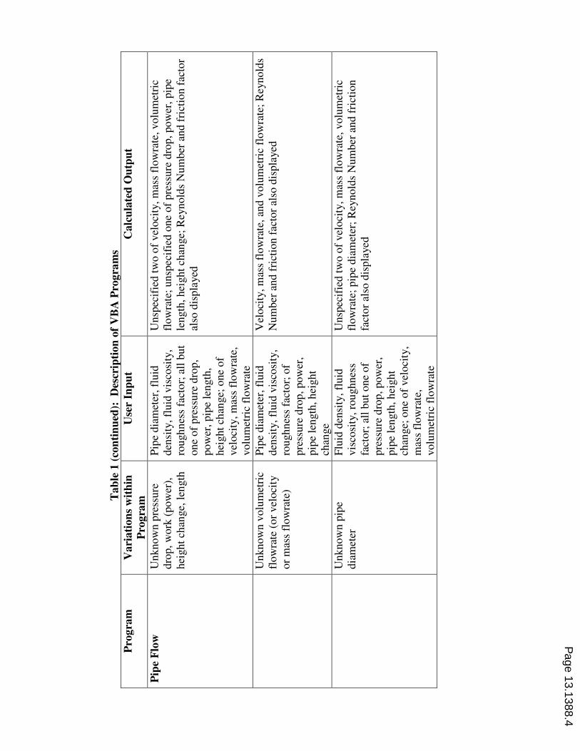
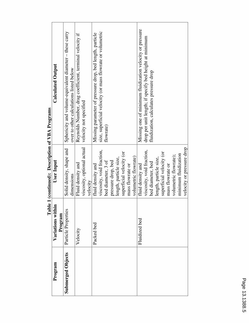
Description of Programs

Table 1 summarizes the programs that will be available for demonstration. Additional details

of each program follow.

Separation in Dilute Systems

The relationships used are the Kremser equation1

1*

,,

*,,

1

1+−

−=

−

−

NoutAinA

outAoutA

A

A

yy

yy (1)

if A = 1

1

1*

,,

*,,

+=

−

−

Nyy

yy

outAinA

outAoutA (2)

Page 13.1388.2

Tab

le 1

: D

escr

ipti

on

of

VB

A P

rogra

ms

Pro

gra

m

Vari

ati

on

s w

ith

in

Pro

gra

m

Use

r In

pu

t C

alc

ula

ted

Ou

tpu

t

Sep

ara

tion

in

Dil

ute

Sy

stem

s

Ab

sorp

tion

(o

r

Str

ippin

g)

– s

taged

syst

ems

(Kre

mse

r)

Anto

ine

const

ant

(fo

r

Rao

ult

’s L

aw)

or

Hen

ry’s

Law

Const

ant,

feed

flo

wra

te a

nd m

ole

frac

tion, so

lven

t in

let

mole

fra

ctio

n

An

y o

ne

of

the

foll

ow

ing i

f oth

er t

wo a

re s

pec

ifie

d:

abso

rpti

on

(st

rippin

g)

fact

or,

fee

d s

trea

m o

utl

et m

ole

frac

tion, n

um

ber

of

stag

es –

if

Rao

ult

’s L

aw u

sed,

can

calc

ula

te o

ne

of

tem

per

ature

, pre

ssu

re, so

lven

t ra

te i

f oth

er

two a

re s

pec

ifie

d

A

bso

rpti

on

(o

r

Str

ippin

g)

–

conti

nu

ous

syst

ems

(Colb

urn

)

Anto

ine

const

ant

(fo

r

Rao

ult

’s L

aw)

or

Hen

ry’s

Law

Const

ant,

feed

flo

wra

te a

nd m

ole

frac

tion, so

lven

t in

let

mole

fra

ctio

n

An

y o

ne

of

the

foll

ow

ing i

f oth

er t

wo a

re s

pec

ifie

d:

abso

rpti

on

(st

rippin

g)

fact

or,

fee

d s

trea

m o

utl

et m

ole

frac

tion, n

um

ber

of

tran

sfer

unit

s – i

f R

aoult

’s L

aw u

sed,

can c

alcu

late

one

of

tem

per

ature

, pre

ssure

, so

lven

t ra

te i

f

oth

er t

wo a

re s

pec

ifie

d

Hea

t E

xch

an

ger

s D

esig

n

7 o

f 8 o

f 4 i

nle

t an

d

ou

tlet

tem

per

ature

s, 2

flo

wra

tes,

2 h

eat

capac

itie

s, s

hel

l/tu

be

confi

gu

rati

on;

opti

onal

ov

eral

l hea

t tr

ansf

er

coef

fici

ent

Mis

sing o

ne

of

4 i

nle

t an

d o

utl

et t

emper

ature

s, 2

flo

wra

tes,

2 h

eat

cap

acit

ies;

par

amet

ers

P, R

, an

d L

MT

D c

orr

ecti

on

fact

or

(F),

are

a ca

lcula

ted i

f over

all

hea

t tr

ansf

er c

oef

fici

ent

pro

vid

ed

P

erfo

rman

ce

area

, ov

eral

l hea

t

tran

sfer

coef

fici

ent,

2

flo

wra

tes,

2 h

eat

capac

itie

s, 2

inle

t

tem

per

ature

s, s

hel

l/tu

be

confi

gu

rati

on

P, R

, L

MT

D c

orr

ecti

on

fac

tor

(F),

2 o

utl

et t

emper

ature

s

Page 13.1388.3

Ta

ble

1 (

con

tin

ued

): D

escr

ipti

on

of

VB

A P

rog

ram

s

Pro

gra

m

Vari

ati

on

s w

ith

in

Pro

gra

m

Use

r In

pu

t C

alc

ula

ted

Ou

tpu

t

Pip

e F

low

U

nkno

wn p

ress

ure

dro

p, w

ork

(pow

er),

hei

ght

chan

ge,

len

gth

Pip

e dia

met

er, fl

uid

den

sity

, fl

uid

vis

cosi

ty,

roughn

ess

fact

or;

all

but

on

e of

pre

ssu

re d

rop

,

po

wer

, pip

e le

ngth

,

hei

ght

chan

ge;

one

of

vel

oci

ty, m

ass

flow

rate

,

vo

lum

etri

c fl

ow

rate

Unsp

ecif

ied t

wo o

f vel

oci

ty, m

ass

flow

rate

, volu

met

ric

flow

rate

; u

nsp

ecif

ied o

ne

of

pre

ssure

dro

p, pow

er,

pip

e

length

, hei

ght

chan

ge;

Rey

nold

s N

um

ber

and f

rict

ion f

acto

r

also

dis

pla

yed

U

nkno

wn v

olu

met

ric

flo

wra

te (

or

vel

oci

ty

or

mas

s fl

ow

rate

)

Pip

e dia

met

er, fl

uid

den

sity

, fl

uid

vis

cosi

ty,

roughn

ess

fact

or;

of

pre

ssure

dro

p, pow

er,

pip

e le

ngth

, h

eight

chan

ge

Vel

oci

ty, m

ass

flow

rate

, an

d v

olu

met

ric

flow

rate

; R

eynold

s

Num

ber

an

d f

rict

ion f

acto

r al

so d

ispla

yed

U

nkno

wn p

ipe

dia

met

er

Flu

id d

ensi

ty, fl

uid

vis

cosi

ty, ro

ughnes

s

fact

or;

all

but

one

of

pre

ssure

dro

p, pow

er,

pip

e le

ngth

, h

eight

chan

ge;

on

e o

f vel

oci

ty,

mas

s fl

ow

rate

,

vo

lum

etri

c fl

ow

rate

Unsp

ecif

ied t

wo o

f vel

oci

ty, m

ass

flow

rate

, volu

met

ric

flow

rate

; p

ipe

dia

met

er;

Rey

nold

s N

um

ber

and f

rict

ion

fact

or

also

dis

pla

yed

Page 13.1388.4

Ta

ble

1 (

con

tin

ued

): D

escr

ipti

on

of

VB

A P

rog

ram

s

Pro

gra

m

Vari

ati

on

s w

ith

in

Pro

gra

m

Use

r In

pu

t C

alc

ula

ted

Ou

tpu

t

Su

bm

erged

Ob

ject

s P

arti

cle

Pro

per

ties

S

oli

d d

ensi

ty, sh

ape

and

dim

ensi

ons

Spher

icit

y a

nd v

olu

me-

equiv

alen

t dia

met

er –

thes

e ca

rry

over

to o

ther

cal

cula

tion

s li

sted

bel

ow

V

eloci

ty

Flu

id d

ensi

ty a

nd

vis

cosi

ty, o

pti

onal

act

ual

vel

oci

ty

Rey

nold

s N

um

ber

, dra

g c

oef

fici

ent,

ter

min

al v

elo

city

if

vel

oci

ty n

ot

spec

ifie

d

P

acked

bed

fl

uid

den

sity

and

vis

cosi

ty, v

oid

fra

ctio

n,

bed

dia

met

er, 3 o

f

pre

ssure

dro

p, bed

length

, par

ticl

e si

ze,

super

fici

al v

elo

city

(or

mas

s fl

ow

rate

or

vo

lum

etri

c fl

ow

rate

)

Mis

sing p

aram

eter

of

pre

ssure

dro

p, bed

len

gth

, p

arti

cle

size

, su

per

fici

al v

eloci

ty (

or

mas

s fl

ow

rate

or

volu

met

ric

flow

rate

)

F

luid

ized

bed

fl

uid

den

sity

and

vis

cosi

ty, v

oid

fra

ctio

n,

bed

dia

met

er, b

ed

length

, par

ticl

e si

ze,

super

fici

al v

elo

city

(or

mas

s fl

ow

rate

or

vo

lum

etri

c fl

ow

rate

);

min

imum

flu

idiz

atio

n

vel

oci

ty o

r p

ress

ure

dro

p

Mis

sing o

ne

of

min

imu

m f

luid

izat

ion v

eloci

ty o

r p

ress

ure

dro

p p

er u

nit

len

gth

; if

spec

ify b

ed h

eight

at m

inim

um

fluid

izat

ion, ca

lcula

tes

pre

ssure

dro

p

Page 13.1388.5

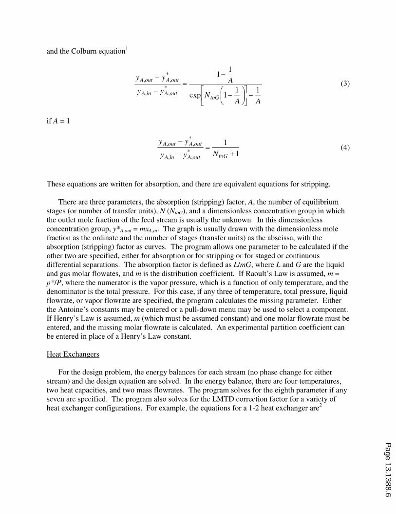
and the Colburn equation1

AAN

A

yy

yy

toGoutAinA

outAoutA

111exp

11

*,,

*,,

−

−

−

=−

− (3)

if A = 1

1

1*

,,

*,,

+=

−

−

toGoutAinA

outAoutA

Nyy

yy (4)

These equations are written for absorption, and there are equivalent equations for stripping.

There are three parameters, the absorption (stripping) factor, A, the number of equilibrium

stages (or number of transfer units), N (NtoG), and a dimensionless concentration group in which

the outlet mole fraction of the feed stream is usually the unknown. In this dimensionless

concentration group, y*A.out = mxA,in. The graph is usually drawn with the dimensionless mole

fraction as the ordinate and the number of stages (transfer units) as the abscissa, with the

absorption (stripping) factor as curves. The program allows one parameter to be calculated if the

other two are specified, either for absorption or for stripping or for staged or continuous

differential separations. The absorption factor is defined as L/mG, where L and G are the liquid

and gas molar flowates, and m is the distribution coefficient. If Raoult’s Law is assumed, m =

p*/P, where the numerator is the vapor pressure, which is a function of only temperature, and the

denominator is the total pressure. For this case, if any three of temperature, total pressure, liquid

flowrate, or vapor flowrate are specified, the program calculates the missing parameter. Either

the Antoine’s constants may be entered or a pull-down menu may be used to select a component.

If Henry’s Law is assumed, m (which must be assumed constant) and one molar flowrate must be

entered, and the missing molar flowrate is calculated. An experimental partition coefficient can

be entered in place of a Henry’s Law constant.

Heat Exchangers

For the design problem, the energy balances for each stream (no phase change for either

stream) and the design equation are solved. In the energy balance, there are four temperatures,

two heat capacities, and two mass flowrates. The program solves for the eighth parameter if any

seven are specified. The program also solves for the LMTD correction factor for a variety of

heat exchanger configurations. For example, the equations for a 1-2 heat exchanger are2

Page 13.1388.6

( )

+++−

+−+−

−

−

−+

=

112

112

ln1

1

1ln1

2

2

2

RRP

RRP

R

RP

PR

F (5)

and for R = 1

( )

−−

+−−

=

222

222ln1

2

PP

PPP

PF (6)

where

inin

inout

tT

ttP

−

−= (7)

inout

outin

shellpshell

tubeptube

tt

TT

Cm

CmR

−

−==

,

,

&

& (8)

where m&is the mass flowrate of the stream, Cp is the heat capacity of the stream, t is the

temperature in the tube, and T is the temperature in the shell.

If the overall heat transfer coefficient is specified, the area is also calculated. As an

alternative, the temperature parameters, usually denoted R and P, may be the input; in this case

the energy balance is ignored and only the LMTD correction factor is calculated. There is no

allowance for phase changes, since the LMTD correction factor is one for these cases (for a pure

component).

For the performance problem, the flowrates, heat capacities, inlet temperatures, area, and

overall heat transfer coefficient are the inputs. The program calculates the outlet temperatures

for a specified heat exchanger configuration. (See the screen shot in Figure 5 in the appendix for

the different configurations included.)

Screen shots for an example problem are shown in the appendix.

Pipe Flow

For pipe flow, the mechanical energy balance (MEB) and a curve fit for the friction factor (f)

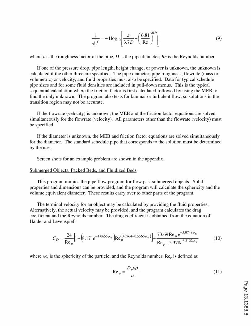
are solved simultaneously. The chosen curve fit is the Pavlov equation3

Page 13.1388.7

+−=

9.0

10Re

81.6

7.3log4

1

Df

ε (9)

where ε is the roughness factor of the pipe, D is the pipe diameter, Re is the Reynolds number

If one of the pressure drop, pipe length, height change, or power is unknown, the unknown is

calculated if the other three are specified. The pipe diameter, pipe roughness, flowrate (mass or

volumetric) or velocity, and fluid properties must also be specified. Data for typical schedule

pipe sizes and for some fluid densities are included in pull-down menus. This is the typical

sequential calculation where the friction factor is first calculated followed by using the MEB to

find the only unknown. The program also tests for laminar or turbulent flow, so solutions in the

transition region may not be accurate.

If the flowrate (velocity) is unknown, the MEB and the friction factor equations are solved

simultaneously for the flowrate (velocity). All parameters other than the flowrate (velocity) must

be specified.

If the diameter is unknown, the MEB and friction factor equations are solved simultaneously

for the diameter. The standard schedule pipe that corresponds to the solution must be determined

by the user.

Screen shots for an example problem are shown in the appendix.

Submerged Objects, Packed Beds, and Fluidized Beds

This program mimics the pipe flow program for flow past submerged objects. Solid

properties and dimensions can be provided, and the program will calculate the sphericity and the

volume equivalent diameter. These results carry over to other parts of the program.

The terminal velocity for an object may be calculated by providing the fluid properties.

Alternatively, the actual velocity may be provided, and the program calculates the drag

coefficient and the Reynolds number. The drag coefficient is obtained from the equation of

Haider and Levenspiel4

( ) ( )[ ]w

w

ww

e

eeC

p

pp

pD ψ

ψψψ

2122.6

0748.55565.00964.00655.4

378.5Re

Re69.73Re171.81

Re

24

+++=

−+−

(10)

where ψw is the sphericity of the particle, and the Reynolds number, Rep is defined as

µ

ρvDpp =Re (11)

Page 13.1388.8

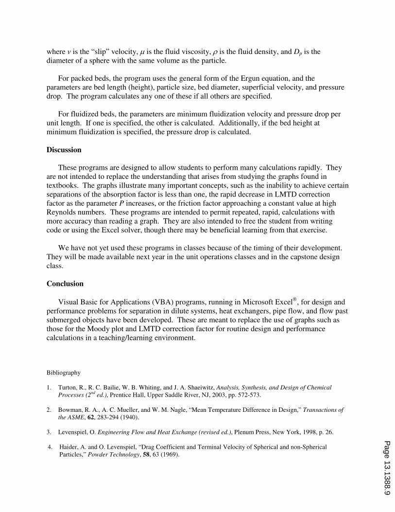
where v is the “slip” velocity, µ is the fluid viscosity, ρ is the fluid density, and Dp is the

diameter of a sphere with the same volume as the particle.

For packed beds, the program uses the general form of the Ergun equation, and the

parameters are bed length (height), particle size, bed diameter, superficial velocity, and pressure

drop. The program calculates any one of these if all others are specified.

For fluidized beds, the parameters are minimum fluidization velocity and pressure drop per

unit length. If one is specified, the other is calculated. Additionally, if the bed height at

minimum fluidization is specified, the pressure drop is calculated.

Discussion

These programs are designed to allow students to perform many calculations rapidly. They

are not intended to replace the understanding that arises from studying the graphs found in

textbooks. The graphs illustrate many important concepts, such as the inability to achieve certain

separations of the absorption factor is less than one, the rapid decrease in LMTD correction

factor as the parameter P increases, or the friction factor approaching a constant value at high

Reynolds numbers. These programs are intended to permit repeated, rapid, calculations with

more accuracy than reading a graph. They are also intended to free the student from writing

code or using the Excel solver, though there may be beneficial learning from that exercise.

We have not yet used these programs in classes because of the timing of their development.

They will be made available next year in the unit operations classes and in the capstone design

class.

Conclusion

Visual Basic for Applications (VBA) programs, running in Microsoft Excel

, for design and

performance problems for separation in dilute systems, heat exchangers, pipe flow, and flow past

submerged objects have been developed. These are meant to replace the use of graphs such as

those for the Moody plot and LMTD correction factor for routine design and performance

calculations in a teaching/learning environment.

Bibliography

1. Turton, R., R. C. Bailie, W. B. Whiting, and J. A. Shaeiwitz, Analysis, Synthesis, and Design of Chemical

Processes (2nd

ed.), Prentice Hall, Upper Saddle River, NJ, 2003, pp. 572-573.

2. Bowman, R. A., A. C. Mueller, and W. M. Nagle, “Mean Temperature Difference in Design,” Transactions of

the ASME, 62, 283-294 (1940).

3. Levenspiel, O. Engineering Flow and Heat Exchange (revised ed.), Plenum Press, New York, 1998, p. 26.

4. Haider, A. and O. Levenspiel, “Drag Coefficient and Terminal Velocity of Spherical and non-Spherical

Particles,” Powder Technology, 58, 63 (1969).

Page 13.1388.9

Appendix – Examples with Screen Shots Illustrating VBA Programs

Example 1

Hot water at 43°C flows from an open, constant-level tank through 2 in schedule 40 steel pipe,

from which is emerges to the atmosphere 12.2 m below the level in the tank. The equivalent

length of the piping system is 45.1 m. Calculate the flowrate.

This problem requires simultaneous solution of a friction factor equation and the mechanical

energy balance, with the velocity as the unknown. Karman plots (f vs. Re×f 0.5

) have also been

used to solve this type of problem (Bennett, C. O., and J. E. Myers, Momentum, Heat, and Mass

Transfer (3rd

ed.), New York, McGraw Hill, 1982, p. 205.). The program solves the two

equations simultaneously and provides the velocity, mass flowrate, volumetric flowrate, friction

factor, and Reynolds number.

Page 13.1388.10

Input screen:

Page 13.1388.11

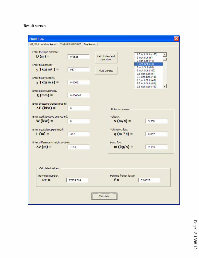
Result screen

Page 13.1388.12

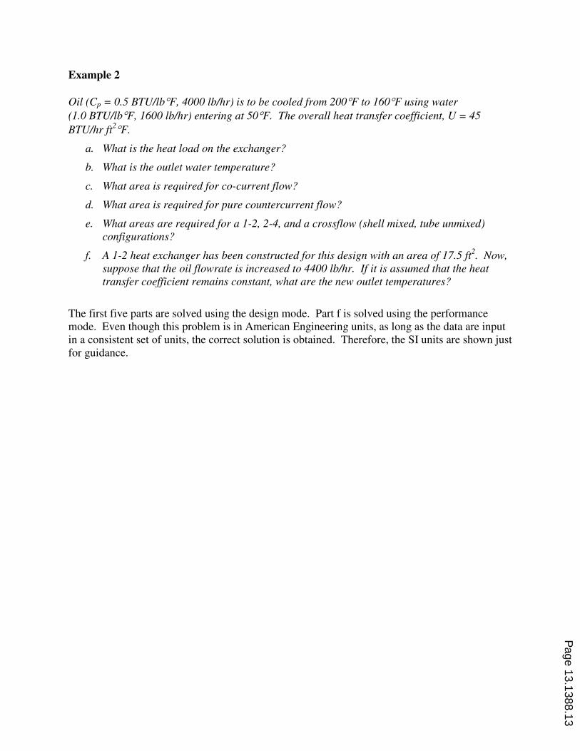
Example 2

Oil (Cp = 0.5 BTU/lb°F, 4000 lb/hr) is to be cooled from 200°F to 160°F using water

(1.0 BTU/lb°F, 1600 lb/hr) entering at 50°F. The overall heat transfer coefficient, U = 45

BTU/hr ft2°F.

a. What is the heat load on the exchanger?

b. What is the outlet water temperature?

c. What area is required for co-current flow?

d. What area is required for pure countercurrent flow?

e. What areas are required for a 1-2, 2-4, and a crossflow (shell mixed, tube unmixed)

configurations?

f. A 1-2 heat exchanger has been constructed for this design with an area of 17.5 ft2. Now,

suppose that the oil flowrate is increased to 4400 lb/hr. If it is assumed that the heat

transfer coefficient remains constant, what are the new outlet temperatures?

The first five parts are solved using the design mode. Part f is solved using the performance

mode. Even though this problem is in American Engineering units, as long as the data are input

in a consistent set of units, the correct solution is obtained. Therefore, the SI units are shown just

for guidance.

Page 13.1388.13

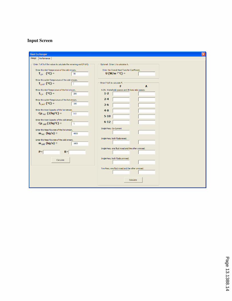
Input Screen

Page 13.1388.14

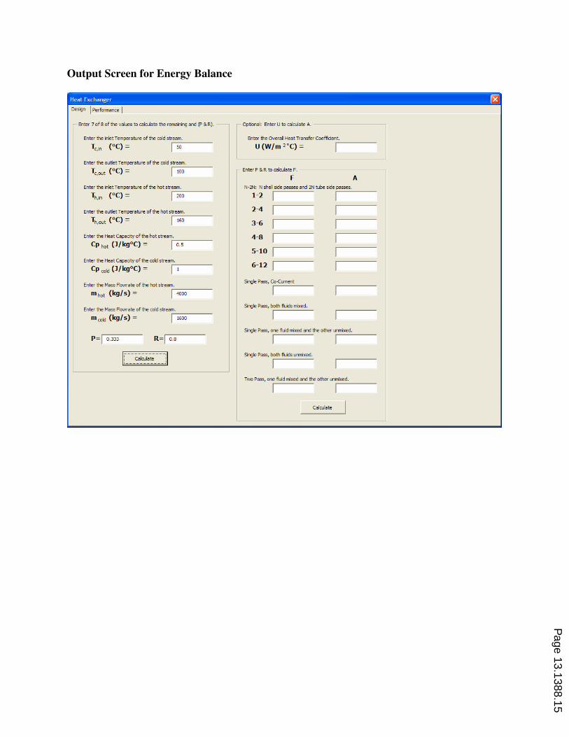
Output Screen for Energy Balance

Page 13.1388.15

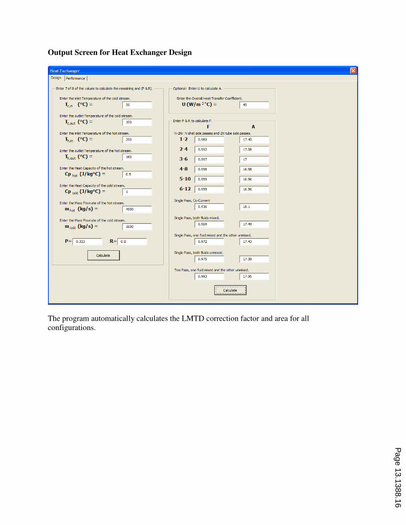
Output Screen for Heat Exchanger Design

The program automatically calculates the LMTD correction factor and area for all

configurations.

Page 13.1388.16

Input Screen for Part f, A Performance Calculation

The performance problem is only solved for a chosen configuration. Here, the radio button for a

1-2 heat exchanger is checked.

Page 13.1388.17

Output Screen for Performance Problem

Page 13.1388.18