VIRGINIA DIVISION OF MINER AL RESOURCES OPEN-FILE REPORT 88-1

VIRGINIA INSTITUTE OF MARINE SCIENCE CONTRIBUTION NO. 1425

RECONNAISSANCE OF ECONOMIC HEAVY MINERALS OF THE

VIRGINIA I NNER CONTINENTAL SHELF

C. R. Berqulat, Jr . and C. H. Hobba, Ill

.l

Prepared In cooperation with the

U. s . Mlnerela Man agement Servlcea, and

VIrgi ni a Subaqueoua Mlnerala ind Materlala Study Commlulon

-

-

--

--

-

Reconnaissance of Economic Heavy Minerals of the Virginia Inner Continental Shelf

by

C.R. Berquist. Jr. Virginia Department of Mines. Minerals and Energy

Division of Mineral Resources Charlottesville. Virginia 22903

C.H. Hobbs. III Virginia Institute of Marine Science

School of Marine Science College of William and Mary

Gloucester Point. Virginia 23062

January 1988

This study was funded in part by the Minerals Management Service. United States Department of the Interior. Cooperative Agreement No. 14 12-0001-30296 to the University of Texas at Austin. Austin. Texas and under a subagreement through the Texas Bureau of Economic Geology to the Virginia Division of Mineral Resources and the Virginia Institute of Marine Science. This study was also funded by the Virginia Subaqueous Minerals and Materials Study Commission. This document is the interim report to that commission on the first year project (July 1. 1986 to June 30. 1987).

Contribution No. 1425. Virginia Institute of Marine Science. School of Marine Science. College of William and Mary. Gloucester Point. Virginia.

-

CONTENTS

Contents . . • • . Figures Tables . Abstract Introduction . . .•..... Geophysical methods and analysis •

Introduction .•..... Field instrumentation •• Individual sites .

Mineral analysis methods ...• Introduction ...... . Sample preparation .. .

Sample concentration Heavy-liquid separation ..... . Magnetic separation ..

Mineral identification • Data base. . . • . . • . ..

Results. . . . . . . . . . . . ........ . Sample composition ••.. Economic potential

Conclusions ...... . Acknowledgments References cited . Glossary . Appendices ..••..•...

1 : II:

III:

IV: v:

Location of samples •• General characteristics of samples • A: MMS cores ••.... B: Commonwealth grab samples. C: Commonwealth (USGS) cores .. Mineral composition of samples ........•• A: MMS cores . • . . . . . . B: Commonwealth grab samples. C: Commonwealth (USGS) cores. Summary composition statistics for all samples • Selected mineral composition with respect to the entire sample ...••......••

i i

Page i i

i i i i i i iv 1 3 3 3 4

15 15 15 15 17 17 18 19 20 20 21 25 25 27 28 30 30 39 39 41 44 46 47 53 62 68

69

-

...

-..

-..

-

ABSTRACT

The Virginia Division of Mineral Resources and the Virginia Institute of Marine Science acquired and analyzed records of 88 nautical miles of seismic and sidescan surveys and 222 grab and core samples from the Virginia inner continental shelf. The project was supported through combined funding from the U.S. Minerals Management Service and the Commonwealth of Virginia (Subaqueous Minerals and Materials Study Commission) to investigate economic heavy minerals offshore of Virginia.

Procedures used to determine heavy mineral concentrations were designed to provide information helpful to mineral industries. The average weight of a sample was 20 pounds. Some samples were derived from processing 5-foot (average) vibracore sections. Concentration of heavy minerals was done with a three-turn spiral and tetrabromoethane. The sand­size fraction of the heavy minerals was estimated from six magnetically separated subtractions by using transmitted- and reflected-light microscopes •

Concentrations of one or more minerals from 33 samples surpassed typical values for economic land-based deposits. The threshold values of the heavy mineral fraction that were used are: ilmenite. 45 percent: leucoxene. 5 percent: rutile. 2 percent: zircon. 5 percent; staurolite. 20 percent: monazite. 1 percent: and a total heavy mineral <THM) concentration of 4 percent. The THM concentration for all samples averaged 3.5 percent and the highest value was 14.7 percent. Offshore sediments sampled by vibracoring are probably Holocene in age and average about 30 feet in thickness. Core penetration into underlying Pleistocene or Tertiary sediments was not attained. High concentrations of THM. ilmenite. zircon. and. to a lesser extent. rutile and monazite support the conclusion that economic mineral occurrences exist on the inner continental shelf of Virginia and suggest that further exploration is justified.

iv

-

----

-...

~ 75°55

Chesn.pcnke

Bny

VA ··-·· NC

• <¢0

0

0

... . .

.. .

. .

. .....

.®

. /.·"· CD . . '

·. ·,·""'· . ' .

EXPLANATION

grab sample

..

0 0

o vibracore geophysical line

1 Assateague-Chincoteague line

4 Smith Island line 6 Virginia Beach lines 7 Bay mouth lines

~"::-::::! geophysical grid (several closely-spaced lines)

2 Wachapreague 3 Quinby 5 Smith Island (hidden

within core sites)

nautical miles 0 5 10 I •, ----'-1 0 10 20

kilometers

Figure l. Location of samples and geophysical tracklines.

2

-

..

-

..

hard copy of the seismic data on electrostatic paper. The adjustable sweep rate of the recorder sets both the repetition rate of the transceiver and the scale of the hard copy.

The sidescan sonar. an EG&G Model SMS 960. is an advanced system sonar that produces nearly planimetrically correct images of the sea floor. The system uses a Model 272 towfish that transmits and receives a 105 kHz acoustic signal in an arc that is normal to the trackline. During the work for this project. the system was set to scan 100 meters (approximately 330 ft) to each side of the towfish. The system's chart-paper rate of advance is adjustable and is automatically scaled to the speed of the vessel. When operating in the 100-m half-width. the image is set at a scale of 1:10.000.

As noted elsewhere in this report. the strength of the reflected signal is indicative of the character of the bottom. Strong reflections. dark areas on the record. result from solid objects. indurated sediments. or bedforms oriented so as to reflect the acoustic signal directly toward the transducer. Light areas on the record result from poor reflection caused by absorption of the acoustic signal by fine-grained soft sediments. scattering of the returned signal. or shadow zones behind raised areas.

To create mosaics of the sidescan images. to determine the speed of the ship over the bottom (to set the sidescan's chart speed). and to be able to return to specific sites. it is necessary to have an accurate and precise navigational system that functions in real time. The R/V Langley is equipped with a Northstar 6500 LORAN e receiver-processor. LORAN-e is the standard. general-service navigational system for coastal waters. The microprocessor and peripheral additions allow real-time calculations of latitude and longitude (by proprietary software within the microprocessor). speed over the bottom. heading. and other information. The LORAN-e coordinates (time delays) and the other data may be printed automatically on associated equipment.

INDIVIDUAL SITES --The Smith Island Grid (Figure 1) was the subject of an earlier

report (Berquist and Hobbs. 1986) and will not be discussed in detail. The sidescan mosaic of the Quinby Grid (Figure 2) is nearly featureless. The only significant variation on the otherwise uniform sonographs is caused by a topographically generated increase in reflection along the eastern portion of the grid. There are one or two minor variations in reflection that are apparently caused by minor changes in bottom topography. The seismic profiles (Figures 3a and 3b) indicate a relatively hard bottom. because there is little penetration of the acoustic signal. In some sections. there are indications that the surface layer of Holocene material over older sediments is approximately 5 meters thick.

The Wachapreague Grid (Figure 1) is somewhat more informative. The interpretation of the sidescan data (Figure 4) shows a number of features that generally follow the changes in bottom topography. The seismic profiles (Figure 5) also depict the bottom topography. These data indicate the relationship between the sidescan imagery and the bottom morphology.

4

""

I • i i • i • I • I

:1 SL 10

3~ ---- '-

15 :r ~_/ 20 25

f __ L__ _ ____ _L__ ___ ~- I..____ I

E 3p

lSL ' 4

3 30

45 so ss 6P

~r SL - - - - - - - - -

30

Q I I I I 5))0 I I I I IQ.OO

SL = Sea Level

J.Q._ Fix Points

meters

QUINBY GRID SEISMIC

LINES 1-4 PROFILES

Figure 3a. Interpreted subbottom profiles from the Quinby grid.

•

..

-

--...

-

--

-

--

-

Some of the sidescan features. particularly those in the northwestern corner of the mosaic, however. do not appear to have a direct relation to the topography. They may be related to the hardness of the bottom or the roughness of the bottom sediment.

The bottom topography at the Wachapreague site exposes underlying stratigraphy. As determined from seismic data in the northernmost line of the grid between fixes 11 and 12. a separate stratigraphic unit appears at the abrupt 2 to 3-meter rise. Similar relationships are evident throughout the area where profiles were obtained. Heavy-mineral concentrations in surficial samples from this site could be representative of different subsurface strata.

A single track line offshore of Assateague and Chincoteague shows that similarly complex patterns exist in the subbottom profiles and sidescan sonographs (Figure 6). The ridgelike features in the bottom topography in this area appear to be composed of discrete sedimentary units.

The reconnaissance seismic survey off Virginia Beach (Figures 7 and 8) shows several acoustic layers between 2 and 5 meters thick. Individual topographic features appear to be confined to specific strata: however. the relationships among elevation (altitude). bottom form. and stratigraphy appear to be better defined than in other locations. Thus. surficial samples may be useful when taken in the specific context of their bathymetric and stratigraphic setting.

The single seismic line off Smith Island (Figure 9) is relatively uninformative. The bottom sediments are hard and so tightly packed that very little of the acoustic signal was able to penetrate the bottom.

8

I

!-' 0

l i ' I • • l ' I • • •

4~

------64 50

~·~-- --=- ----65 81

9~ 8

9 IJI

.c:::::- -~=-======== -j ------

~

SEISMIC PROFILES WACHAPREAGUE GRID J.Q... Fi;( Points

Q 1 1 1 1 rn ! , o o 190 0 5x vert. ex.

Figure 5. Interpretation of the Wachapreague grid subbottom profiles.

-

-

-....

-

-

-+-

·73 \ \

., 70

'· -·-.... TRACKLINE

\70 \ \ \

I() I{) 0 I{)

r--

WITH FIX NUMBERS

+

. \

I :~58 \ \ . \ . I \ \

SEISMIC SURVEY

VIRGINIA BEACH

+

• \ . \ •

42 \ I I ·--. -.+, +

\ •, ·-·-·--~~ ._

-~. 2.o ...... -.-·- ·-z~ ·:_:-- ·-......, 30 '-.) -. --.., ' Figure 7. Subbottom tracklincs off Virginia Beach. ........

12

1--' ~

or: 10 en .....

w -w 20l..E

0 0

I

10 'l:t 0

SEISMIC PROFILE

S. L ::: Seo Level ...ill... Fi Jt Points

0 4 n. mi I I I ,. - ,. -,

0 5 km

0 rCl 0

• ~. :.: t

~·J

.... ~-;i ~ ~ ..... :~ N

~~ .... .)·' . ,~ '- . . ... C:Jv ,· .. -· ' '.;;;:· .. ' ~·-... · .

. '),_ .. : :·: .:7. ""'- ""'"' • • .; 111 ~' :..~···

r:::."- . : ,.,~· :-5~ "1· ·:.!

·, .... ::.:) ~!··!

t

10 0

- ... - - .......... - ..

SEISMIC

~~ .... ~q,.·

:,..:

0 0 2

I

Figure 9. Interpretation of new seismic line off Smith Island.

I

-

LINE

10 -a­(])

0

j i

~ (])

0

Octo be r 8 l I 9 8 6

<r:> 'ho tiL 00)

~

' J

I()

s

~

...

-

...

-

FLOW CHART FOR MINERAL SEPARATION AND ANAlYSIS·

t W£10'i

DAY AT 10• (;

Wf~H WAHflt C:O-.fU'!!T • ~~~ ... , o.., Wtoitl'ld+fWet '*'•• ... tJ

l!GHJI

.... I

Vllf

01~~ -- 00¥

I Wf!CH

W..IGH

I

PAUII{Vl

HUVV ltOUIO ft.J,I.?, fllliiiAitltQMOffHAN(I

IUAfltAfJON

=

I MfAVV liOUIO

IOAf'fATJON fO OtlfiiiiMINI

"HlAVIU OISCAfltO Oil AftCHfVI Hfl.O JH ltCHfl

~~ OISC~ ~

p,(J\.QNlflC

M40NlTIC

ftf:OH

AJ!fAI.VZt! FOR tNOIVIOUAl, MJNf AAl

SPICIU f -201 I

Wf!GH

I ANAl 't'lt r0111

INOIVIOtJAl Ml!lrffRAl $P'!CIU I -.JOS t

W(IGHT I

Olftii!MIJ!f( W'T. '1. HlAVIU

I tH~A"O 0111

AACHWl

=

VUUtCAl. MAQNtTtC lti'Afii:AliON Af tU AIM'S

VfRTICAl MAGNUIC III"AIU.TION AT O.J .......

I"'CtiNtD MAGNlfiC

w,~c-------.....::::c:'===---r I

ANAl Vlf FOI' I~OlVfOUAl MINfJII:Al

$1"(CfU I - )Of I

W'UOH VtlllfiCAI. MAQNffiC I h:I"AftAtfOH AT 1 I AWl HOlD 'Oft

CHfMICAL AJrfAl Yltt

~;_v"~~,r~~o WAQfrfiJtC UI"ARAl'fOH

YtRTtCAC. ._.ONtTU: .tfi"AftA'fiON ~'f 1.t .....

I ___ _JMA~Q~N~lt~~~-------------~

~ ~ YfftTtCAl MA(Jirtffte

III•AJIIlAHON AT t.l AWl

L----~M~A~O~N~IT~I~C-------------~~ ..

~ VUffCAl MAONtTtC

tii"ARATlOfoil AT 1.1 A ....

~ MAGHUIC:

Vfllllllea.&.. MAGNfliC UI"A.AATION AT t.l #IMJIS

'-----M~A~G~N~I~TI~C--------------'l~fh. f- ·~

\'UiftCAL MA011(£T!C I(P'AIII'ATION AT t.l AMf>t

MAQNtfJt

~ INCll,£0 M.\ONtTIC

IOA'Ut, TfOftt AT O.J AMr1

" wr

1ow

ANAl 'tl( ,011 ffrfDfVfOUAl MINUtAl

Sl'tCIU C -201)

lkCUNlO MAOHfTtC lrPAftATIOfill "' t.t At.ilrt

W£10H I

ANAlYlf FO" fNOIVIDUAl Mfl'f(II!:AI,

lfl'fClfll -701 I

Figure 10. Flow chart showing the scheme of sample analysis.

-..

-

..

---

-

toward the poles of the separator. The portion of the sample held by the magnet was again run through the vertical Frantz separator but at a setting of 0.7 ampere. The retained fraction (labeled 203) is commonly known as the "hand-magnetic" portion. Minerals not attracted to the magnet were processed through the barrier-type separator. Successive mineral groups were derived from the magnetic fractions of the Frantz separator at 0.2 (labeled "204"). 0.4 (labeled "205"). 0.6 (labeled "206"). and 1.8 amperes (labeled "207"). The last group. the nonmagnetic fraction at 1.8 amperes. and was labeled "208". Each of the six groups was weighed and stored in a glass vial.

MINERAL IDENTIFICATION

Each of the six magnetic fractions (203 to 208) was examined under reflected- and transmitted-light (dissecting and petrographic) microscopes. The minerals in each fraction were identified and their abundances were estimated or counted. The weight of a mineral in each fraction was calculated by multiplying its observed abundance by the weight of the fraction. Because some minerals were present in more than one magnetic fraction. their total abundance was determined by summing their weights in each fraction. Figure 11 is an example of the observations and calculations used to determine the weight percent for the entire sample. Minerals observed. but not listed on Figure 11. were grouped into the "other" category.

The magnetite fraction may contain minerals common to subsequent magnetic fractions. X-ray fluorescence of the 203 fraction of two samples indicated excessive titanium: the excess could be explained by approximately 40 percent titano-magnetite (0. Fordham. personal communication). Because optical identification of different opaque minerals in the 203 fraction was difficult and inconsistent among observers. the entire fraction was labeled "magnetite ...

The 206. 207. and 208 fractions were also examined under high intensity short-wave ultraviolet light. This technique identified monazite (green fluorescence) and zircon (yellow to orange fluorescence) as well as helped to estimate quartz contamination in the 208 fraction.

The mineral composition of each sample is shown in Appendix III. Because quartz was commonly found in the 208 fraction. its weight was included in the heavy mineral fraction rather than the light fraction. It was commonly observed that quartz made up at least 90 percent of the 208 "other" fraction. A correction was made to the weight-percent of the total heavy minerals by subtracting the weight of quartz contamination and was included in the calculation of data under column headings 11 WT% TOTAL HM" in the appendices. The decrease ranged from 2 percent to 18 percent of the uncorrected value and averaged 2.6 percent.

18

•

-

-

...

--

RESULTS

SAMPLE COMPOSITION

Appendix III shows the mineral composition for the heavy mineral fractions of all samples. The data is subdivided into three groups: Commonwealth cores. Commonwealth grab samples. and Minerals Management Service cores. Because the usefulness of relying upon surface grab samples in predicting economic mineral potential is questioned (A. E. Grosz • personal communication). grab sample data were separated from core data for the Commonwealth project. Appendix III includes separate statistics for each of the three groups. Appendix IV shows statistics for all samples treated as one group.

Another way of characterizing mineral abundance is to calculate mineral composition relative to the entire sample rather than to the heavy­mineral fraction. This is shown in Appendix V. The data have been "weighted" by the total heavy-mineral concentration so that mineral abundance per ton. for example. may readily be estimated.

Tables 1 and 2 show average and highest values for the more economic minerals both by group and by all samples. The total heavy-mineral <THM) concentration (average and highest value) of "CW grabs" (Commonwealth acquired grab samples) departed more from "all samples" than did the values for cores. However. mineral concentrations were nearly the same for cores and grab samples. Therefore. grab samples appear to be useful in predicting offshore mineralogy. but they may not be good indicators of total concentration. This hypothesis was only apparent by inspection and has not been statistically tested.

TABLE 1. Average concentrations of selected minerals as a percentage of the heavy-mineral fraction. CW =Commonwealth data. MMS =Minerals Management Service data.

WT % WT % WT % WT % WT % WT % THM ILMENITE LEUCOXENE RUTILE ZIRCON MONAZITE

MMS cores 2.4 23.0 1.2 1.1 3.3 0.2 CW grabs 4.5 28.6 1.7 1.1 2.7 0.3 CW cores 2.9 30.8 1.2 1.2 3. 1 0. 1

a 11 samples 3.5 27.8 1.4 1.2 3. 1 0.2

20

..

Determinations of the "best" samples were based on several criteria. For land deposits. the average THM concentration should be at least 3 to 4 percent. Several samples were noted where THM exceeds this. even though the individual mineral abundance may be less than the threshold values suggested by Garner (1978). These were included because the same volume of a mineral may be available at twice the THM concentration but half the abundance of the heavy-mineral fraction. e.g •• a THM of 5 percent and ilmenite of 60 percent is equivalent to a THM of 10 percent and ilmenite of 30 percent. Also marked were samples with THM values less than 4 percent where certain ECON minerals were in great abundance because these samples may suggest a depositional environment with selective enrichment leading to nearby higher-grade sediments.

As an aid to further assessment of the economic potential of the samples. Appendix V presents the weight percent of selected minerals with respect to the total sample. Garner's values can likewise be converted by multiplying each of the following mineral concentrations by 5 percent: ilmeni 2.25 percent. leucoxene and zircon ~ 0.25 percent. rutile = 0.1 percent. and monazite = 0.05 percent. As previously mentioned. this procedure partially eliminates the concern for THM concentration while searching for high-grade samples.

TABLE 3. Several samples with economic potential selected from Appendix III. Composition is relative to the heavy-mineral fraction. P = present: see Appendix III for additional explanation of tabulated data.

WT % WT % WT % WT % WT % WT % WT % Sample THM IL RUT LEUCX MON ZR ECON

H01 3 5.4 17.4 2.7 0.3 1.4 7.6 32.2 V1-4 0.8 56.2 1.7 3.3 0.3 3.8 66.1 4 9.3 21.4 1.4 3.0 0.2 3.3 30.8 33 5.1 58.8 0.8 0.6 ·0.1 4.1 65.8 54 14.7 29.0 1.1 0.2 0.4 4.5 35.9 59 11.0 34.9 1.5 0.6 0.1 4.3 42.4 85 10.8 54.9 2.4 1.8 0.1 3.8 63.1 1134-1 8.8 34.0 1.8 0.3 0.2 4.6 41.1 1136 1 9.0 28.7 1.1 1.0 p 3.5 34.7

22

-

-

--

EHIIRE SAMPLE

EHTI RE SAHPLE

' ', I

Ul-4

••·~--·o. az THH I -

./ . -.

GRAB tl 4

.3:t. THM

t:==:z:::z::::;:::(..I.EII C 0 X E HE 3 • 3 Y.

I I LE 1. 7%

ILMENITE 56.?.:1.

COMPOSITION UEflVY HI HERA L FRACTION

3.3'% TILE 1.7:t.

I LMEHIIE 21. 4:t.

COMPOSITION HEAVY MINERAL FRACTION

Figure 13. Graphic presentation of selected samples.

24

....

...

-

" ..

..

---...

:~

From Virginia Institute of Marine Science. S. A. Skrabal. L. J. Calliari. S. M. Dydak. and C. T. Fischler cut and logged cores. processed samples. and identified and estimated mineral abundance. C. T. Fischler was responsible for managing the sediment laboratory: her responsibility extended to daily attention to equipment and supply orders. work schedule coordination. and computerized data compilation. R. A. Gammish assisted in sample collection and participated in relevant discussions throughout the projects. Captains C. E. Machen and L. D. Ward. and Mate S. H. George from vessel operations provided expertise in data collection aboard the R/V Langley and R/V Captain John Smith. Many of the surface grab samples were collected from the chartered vessel Anthony Anne with the help of Captain J. A. Penello. Dr. G. P. Burbank of Hampton University performed the heavy­liquid and some magnetic separations under contract from the Virginia Institute of Marine Science.

26

--

...

----

-

-

GLOSSARY

Box-corer: A device to collect a sample of uniform depth across an area approximately 6 by 9 inches. The sampler is driven into the bottom by its own weight and ballast: depending upon the hardness of the bottom. penetration ranges up to 18 inches.

Core. core sample: A sample collected with an aim to acquire information over depth. See box-corer. vibracorer.

Exclusive Economic Zone (EEZ): A zone extending offshore from 3 nautical miles (separating state from federal jurisdiction) to 200 nautical miles in which the federal government has jurisdiction. (Reference Presidential Proclamation No. 5030. 1983)

Frantz magnetic separator: A commercially marketed device used for separating minerals according to their magnetic susceptibility. It is used to aid in the identification of individual mineral species.

Grab sample: A sample taken from the surface of the bottom sediment without concern for the penetration depth or uniformity. Usually grab samples are the most easily obtained samples of the bottom; however. their value is limited to information on the sea bottom only.

Heavy-liquid separation: A laboratory procedure for separating minerals based on their specific gravities (density). Minerals with a density greater than the liquid will sink and minerals with a density less than the liquid will float. "Heavy" liquids used in this process are usually toxic.

Heavy mineral: A detrital mineral having a specific gravity greater than an arbitrary standard (usually around 2.85). Most of the detrital minerals of economic interest are heavy minerals. Note: Heavy minerals should not be confused with heavy metals. When these metals are found in the marine environment in higher than normal concentrations. they are usually anthropogenically introduced pollutants.

Humphrey Spiral: A commercially marketed device for making a rough separation of the heavy minerals from bulk sediment samples.

Magnetic susceptibility: The ratio of induced magnetization to the strength of the magnetic field causing the magnetization. Material that shows no magnetic properties while it is not in a magnetic field may show magnetic properties if placed in a magnetic field.

28

-

APPEND IX I

LOCATION OF SAMPLES

Loran coordinates are slaves of the 9960 chain. Latitude and longitude were obtained from automatic conversion of loran coordinates by the shipboard loran receiver-processor. Data not available are noted by 11*11

MMS VIBRACORES

CORE WATER LORAN C LATITUDE LONGITUDE RECOVERED ,_ NUMBER DEPTH COORDINATES CORE LENGTH

(FT) y X deg min deg min (FEET)

H1 38 41405.1 27132.7 37 05.00 75 45.99 13.5 H2 38 41406.1 27133.8 37 05.12 75 46. 19 15.0 H3 37 41408.0 27134.9 37 05.31 75 46.37 4.5 H4 38 41409.8 27136.1 37 05.50 75 46.58 15.5

." .. H5 34 41412.2 27137.2 37 05.74 75 46.74 6.2 H6 37 41392.9 27131.0 37 03.94 75 46.03 20.4 H7 36 41398.8 27134.9 37 04.56 75 46.70 12.8 .. H8 30 41402.0 27136.7 37 04.89 75 46.98 9.5 H9 32 41405.3 27138.6 37 05.22 75 47.29 6.0 H10 35 41408.5 27137.4 37 05.44 75 46.90 12.1

·- Hll 30 41410.7 27139.3 37 05.69 75 47.25 7.0 H12 29 41411.5 27139.7 37 05.77 75 47.31 7.0 H13 38 41412.8 27140.9 37 05.92 75 47.54 6.8 H14 38 41414.6 27138.8 37 05.99 75 47.01 10.0 H15 30 41413.6 27138.3 37 05.89 75 46.93 2.0 B1 25 41399.5 27202.9 37 07.03 76 01.97 9.5 B2 22 41415.2 27200.0 37 08.20 76 00.74 9.0

... B3 15 41423.1 27200.1 37 08.84 76 00.47 12.5 B4 35 41385.3 27210.2 37 06.13 76 04. 17 6.5 85 25 41369.8 27 210. 1 37 04.87 76 04.71 10.5 V1 48 * ·• * 36 54.53 75 56.56 19.7 V2 46 * * 36 53.15 75 55.29 18.6 V3 49 * * 36 51.80 75 53.84 14.3 V4 52 * * 36 50.51 75 51.55 20.0 V5 * * * 36 54.04 75 56.39 18.8 V6 47 * * 36 52.41 75 50.41 6.4

-30

·-

COMMONWEALTH GRAB SAMPLES. continued

·-GRAB DEPTH LORAN C LATITUDE LONGITUDE NUMBER (FATHOMS) COORD I NATES

y X deg min deg min

41 * 41419.8 27142.7 37 06.56 75.47.70 42 * 41415.1 27139.9 37 06.07 75 47.23 43 * 41446.8 27120.0 37 07. 97 75 41.73 44 * 41447.0 27125.5 37 08.18 75 42.94 45 * 41447.7 27131.9 37 08.46 75 44.32 46 * 41449.6 27134.9 37 08.71 75 44.91 47 * 41466.8 27140.0 37 10.31 75 45.44 48 * 41500.0 27142.0 37 13.09 75 44.71 49 * 41510.1 27134.9 37 13.68 75 42.81 50 * 41539.9 27134.9 37 16.12 75 41.76 51 * 41540.1 27142.0 37 16.37 75 43.30 52 * 41540.1 27145.0 37 16.47 75 43.96 53 * 41560.1 27139.9 37 17.95 75 42.15 54 * 41580.1 27134.9 37 19.42 75 40.35 55 * 41579.9 27125.0 37 19.09 75 38.23 56 * 41610.0 27134.9 37 21.88 75 39.30 57 * 41369.8 27159.9 37 03.10 75 53.31 58 * 41339.9 27154.8 37 00.49 75 53.23 59 * 41284.9 27144.7 36 55.63 75 52.89 60 * 41279.7 27154.9 36 55.60 75 55.39 61 * 41249.6 27154.9 36 53.16 75 56.46 62 * 41241.9 27162.0 36 52.81 75 58.36 63 * 41226.7 27157.4 36 51.40 75 57.84 64 * 41229.9 27155.0 36 51.56 75 57. 18 65 * 41229.9 27144.9 36 51.15 75 54.85 66 * 41209.8 27144.9 36 49.52 75 55.56 67 * 41209.9 27120.0 36 48.51 75 49.83 68 * 41149.9 27109.9 36 43.16 75 49.55 69 * 41149.7 27113.0 36 43.28 75 50.27 ,_ 70 * 41149.9 27115.1 36 43.38 75 50.74 71 * 41159.9 27119.9 36 44.41 75 51.51 72 * 41159.9 27125.1 36 44.64 75 52.72 73 * 41159.7 27129.9 36 44.82 75 53.83 74 * 41160.0 27140.0 36 45.26 75 56.16 75 * 41129.5 27119.0 36 41.88 75 52.33 76 * 41109.9 27119.9 36 40.31 75 53.22 77 * 41089.5 27115.0 36 38.42 75 52.75 78 * 41089.8 27104.9 36 37.99 75 50. 39

·- 79 * 41050.1 27105.0 36 34.72 75 51.73 80 * 41049.9 27101.8 36 34.55 75 50.99 81 * 41049.9 27099.8 36 34.46 75 50.52

32

...

-..

" .. COMMONWEALTH CORES {USGS). continued

CORE LATITUDE LONG !TUDE NUMBER deg min deg min

"- 1103 37 00.55 76 03.35 1106 37 00.72 75 58.70 .. 1107 37 02.34 76 01.00 1109 37 03.75 76 02.00 1111 37 05.62 75 59.80 1116 37 03.42 75 58.69 '- 1119 37 01.55 75 56.58 1120 37 00.70 75 55.48 1121 37 01.60 75 54.30 - 1122 36 59.95 75 52.25 1127 37 02.40 75 50.05 1129 37 03.70 75 46.85 - 1130 37 04.00 75 47.91 1131 37 04.75 75 49.32 1132 37 04.24 75 51.18 1134 37 04.12 75 53.28 1136 37 02.50 75 53.40 1139 37 04.10 75 57.60 2000 36 57.05 76 06.62 2001 36 55.35 76 06.62 2002 36 59.52 76 04.02 110 37 59.25 75 13.34

... 115 38 02.38 7 5 07. 15 116 38 01.44 75 07.08 117 38 00.59 75 01.80

R-

-

...

34

-

I

'81

.B4

w I 0'1

•1109

t:)

,1103

'

,1107

, 1111

-g fa

i i

v-

(?~ •. .

:< .. :·"',·~~.-• • • J. " • ~ ...... :; •

• 1139

.1116

.1119

1106 •

'

/:. -_y . . . . .

• 1121

.1120

c ' • '

~7 38 • 4 •

INSERT A 36 •

•35 -~40

•41 42

.3 H13. • ·~HI5 HI~ • .H5

11• • ·H 4 H3 · H9. HIO•:Hz

.1131 ·H8 ·HI .H7

.1134 •u32 .1130 •H6

.2 ·1129

.57 .I

• 1136 ·1127

0 km 10 b t I 1 l l I I I 1 I I I I I I

n.mi 5 ·o .5"8 ~ ,....

Figure 15. Location of samples at northern entrance to Chesapeake Bay.

•

w co

• 74

• 101

73 72 • • 71 •

7069 68 . • • •

• 75

.76

,77

.100

.78

.79 .sqs~B2.m 84 • ·85

92, ,91 .9,0 .89 88

89A • •87

i & • i

INSERT C

.99 ,98 97

• .96 • 95 .94

km 10 f· t f! It I Ill I l ·' I A 0 n.m1

•86 -o <;t

~ ,....

,93

Figure 17. Location of samples off Virginia Beach to North Carolina.

i l

..

... CHARACTERISTICS OF MMS CORES. continued

<·- CORE CORE DRY % % % WT % SAMPLE NAME LENGTH LENGTH SAMPLE WT sand mud gravel TOTAL HM

(CM) (FT) (GRAMS)

H13-1 204 6.7 8324 93 5 3 2.23 H14-1 148 4.9 5771 * * * 0.52 - H14-2 142 4.7 5942 81 16 4 1.49

V1-1 149 4.9 7513 * * * 1.17 V1 2 151 5.0 7267 * * * 0.82 V1-3 152 5.0 4400 * * * 0.61 V1-4 148 4.9 5245 * * * 0.83 V2-1 113 3.7 4272 * * * 2. 72 V2-2 152 5.0 5530 * * * 1.67 - V2-3 156 5.1 6910 * * * 3.90 V2-4 139 4.6 6593 * * * 2.12 V4-1 190 6.2 4721 * * * 1.77 - V4-2 134 4.4 7979 * * * 1.06 V4-3 163 5.3 4606 * * * 1. 39 V4-4 153 5.0 3766 * * * 1. 35 V3-1 152 5.0 7305 93 5 2 1.42 - V3-2 143 4.7 6432 64 34 2 0.50 V5-1 108 3.5 2317 88 12 0 1. 95 V5-3 155 5.1 5565 95 5 0 1. 26 - V5-4 110 3.6 3610 94 5 1 1. 20 V5 5 128 4.2 6424 90 3 7 1.44 V6-1 147 4.8 5843 94 6 0 2.48

,,. V6-2 148 4.9 7051 91 7 2 1. 71

AVERAGE 146 4.8 6075.4 87.1 11.4 1.5 2.44 STD DEV 33 1.1 1442.5 11.0 10.5 3.2 1.40 - MIN VALUE 86 2.8 2317.0 54.0 0.0 0.0 0.50 MAX VALUE 289 9.5 9853.0 98.0 41.0 19.0 6.88 SUM 8632 283.2 358453. -

number of samples 59

-

40

-

42

...

C. CHARACTERISTICS OF COMMONWEALTH (USGS) CORES

CORE CORE DRY % % % % SAMPLE NAME LENGTH LENGTH SAMPLE WT SAND MUD GRAVEL TOTAL Ht1

(em) (ft) (grams)

1090-1 165 5.41 8649 83 17 0 2.46 1090-2 189 6.20 15448 86 14 0 1. 91 1091-1 150 4.92 10348 85 15 0 2.36 1091-2 150 4.92 11148 85 15 0 1.71 1091-3 170 5.58 13447 78 22 0 1.61 1092-1 236 7.74 14850 91 2 7 1. 70 - 1092-2 242 7.94 10450 89 2 9 1.03 1094-1 158 5.18 14049 92 8 0 1.15 1094-2 179 5.87 13151 76 24 0 1.01 1095-1 160 5.25 12648 87 13 0 2.51 1095-2 150 4.92 12949 91 9 0 2.30 1096-1 150 4.92 11850 87 12 0 1.84 1096-2 150 4.92 13049 73 26 1 2.23 1097 1 200 6.56 17950 93 7 0 2.60 1097-2 180 5.91 16951 76 19 6 1. 39 1097-3 146 4.79 13450 75 22 3 1.26

.... 1098-1 191 6.27 14849 75 0 25 1. 78 1098-2 190 6.23 14051 65 33 2 0.58 1099-1 257 8.43 15550 73 24 3 1.18 1099-2 200 6.56 15849 78 5 17 1. 78 1100-1 162 5.32 12651 94 6 0 2.64 1100-2 180 5.91 16249 88 11 1 2.51 1103-1 160 5.25 7851 84 12 5 1.80 1103-2 125 4.10 4651 69 22 8 1.62 1103-3 215 7.05 12851 93 6 2 1. 74 1106-1 145 4. 76 13450 99 1 0 3.59 1106 151 4.95 14148 99 1 0 2.63 1107-1 165 5.41 15450 99 1 0 4.35 1107-2 167 5.48 15048 98 2 1 1.83 1109-1 238 7.81 11050 91 9 0 3.08 - 1111-1 148 4.86 11450 92 8 0 2.76 1111-2 186 6.10 15110 90 10 0 3.20 1116-1 193 6.33 10850 88 12 0 4.39 - 1116-2 217 7.12 15751 83 14 2 4.00 1119-1 205 6.73 19051 99 1 0 2.43 1119-2 123 4.04 19666 96 4 0 2.39 1120-1 160 5.25 12650 98 2 0 1.95 1120-2 175 5.74 15449 95 4 0 3.05

44

, ..

-

---

-

-

----

.•

APPEND IX II I

MINERAL COMPOSITION OF SAMPLES

Explanation of Tabulated Data

"P" means several grains of the mineral were observed in the entire sample: that is. it was present.

"T" means the mineral was observed to be between 0.5 percent and 1 percent in abundance or in trace quantity.

"ECON" is the sum of the weight percents of ilmenite. rutile. leucoxene. sillimanite/kyanite. monazite. and zircon.

"MAG" (magnetite) contains an undetermined amount of titanomagnetite.

Samples with high concentrations of one or more ECON minerals are underlined

Mineral names not spelled completely in column headings have been abbreviated as follows: IL =ilmenite. MAG= magnetite. GAR garnet. EP =epidote. STAUR =staurolite. AMPHIB =amphiboles. PYROX = pyroxenes. SILL/KY sillimanite and kyanite. TOURM =tourmaline. LEUCOX leucoxene

46

- COMPOSITION OF MMS CORES. continued

WT % WT % WT % WT % WT % WT % SAMPLE NAME TOTAL H~1 MAG IL GAR EP STAUR

VI 1 1.17 2.69 19.44 17.81 8.49 0. 19 - Vl-2 0.82 1.42 50.71 6.69 12.80 2.34 Vl-3 0.61 1.44 45.72 2.54 12.81 3.81 Vl-4 0.83 1.68 56.22 6.29 6.12 1.86 V2-l 2.72 4.07 23.85 15.24 7.40 0.95 - V2-2 1.67 3.09 45.22 9.76 9.11 0.63 V2-3 3.90 0.51 37.16 14.73 15.08 1.95 V2-4 2.12 1.68 50.09 4.82 7.51 0.85

, ... V4-l 1.77 5.72 23.83 12.95 4.96 1. 23 V4-2 1.06 0.85 38.30 9.62 9.92 2.48 V4-3 1. 39 2.21 32.38 10.96 17. 14 1. 35

~-V4-4 1. 35 2.21 45.16 8.87 13.37 1.17 V3-l 1.42 2.34 32.51 12.71 7.18 2.52 V3-2 0. 50 0.81 36.21 3.37 15.10 2.59 V5-l 1. 95 3.03 18.17 15.98 8.77 2.19 V5-3 1.26 1.55 42.75 6.65 12.18 2.97 V5-4 1.20 3.10 44.27 5.72 13.65 1. 81 V5-5 1.44 8.86 45.79 9.50 3.69 2.81

·- V6-1 2.48 6.92 24.09 18.17 4.01 0.35 V6-2 1. 71 4.28 24.97 14.86 7.81 1.44

AVERAGE 2.44 6. 19 23.01 13.39 7.86 1.50 - STD. DEV 1.40 4.19 12.50 4.76 3.07 1.63 MIN VALUE 0.50 0.51 7.65 2.54 2.22 0.00 MAX VALUE 6.88 18.03 56.22 25.41 17.14 6. 72

-

...

48

-COMPOSITION OF MMS CORES. continued

'vJT % WT % WT % WT % WT % WT %

- SAMPLE NAME AMPHIB PYROX RUTILE SILLIKY SPHENE TOURM

V1-1 26.52 6.75 1.58 0.59 0.05 0.51 V1-2 9.07 2.39 1.93 2.20 0.32 0. 73 - V1-3 15.01 2.41 1.37 3.02 0.17 0.06 V1-4 7.82 1. 31 1.69 0.76 0.05 0.98 V2-1 22.27 6.19 0.69 1. 58 0.41 0.52 V2-2 9.26 1.29 2.25 0.75 0.18 0.28 V2-3 12.29 1. 24 1. 25 3.81 0.21 o. 34 V2-4 9.17 2.45 1.62 0.84 0.59 0.16 - V4-1 23.27 8.52 0.50 0.80 0.39 0.62 V4-2 17.60 4.89 2.09 1.43 0.77 0.10 V4-3 15.63 2.40 1. 59 1.89 0.22 0.85 V4-4 9.07 2.14 2.08 1.43 0.25 0.35 V3-1 13.35 5.97 1. 37 1.85 0. 18 0.46 V3-2 21.53 0.98 1.89 3.83 0.28 T V5-1 15.78 8.07 0.91 0.62 0.56 1. 31 - V5-3 13.33 4.25 1.61 2.93 0.43 0.36 V5-4 11.18 2. 11 1. 99 1.17 0.29 1.12 V5-5 6.99 3.55 1.37 1.50 0.13 0.88 V6-1 18.18 4.64 1. 38 0.14 0.17 0.44 - V6-2 20.05 2.34 1.59 0.06 0.03 1. 79

AVERAGE 16.79 6.18 1.13 1. 53 0.55 0.64 STD. DEV 5.76 3.60 0. 57 1.20 0.47 0.49 MIN VALUE 5.24 0.98 0.00 0.06 0.00 0.00 MAX VALUE 26.76 21.82 2.66 5.19 2.04 1. 96

50

-

COMPOSITION OF MMS CORES. continued

WT % WT % WT % WT % WT % SAMPLE NAME LEUCOX MONAZITE ZIRCON OTHER ECON

V1-1 0.71 0.05 3.13 11.50 25.50 V1 2 1. 90 0.36 2.82 4.32 59.92 - V1-3 2.17 0.33 2.74 6.41 55.34 V1-4 3.31 0.29 3.80 7. 81 66.08 V2-1 1.18 0.15 2.21 13.31 29.64 V2-2 1.77 0.04 6.16 10.22 56.19 V2-3 1.80 0.29 2.97 6.38 47.27 V2-4 1.42 0.05 3.66 15. 10 57.68 V4 1 1. 70 0.08 3.06 12.36 29.98 - V4-2 1.86 0.04 2.01 8.04 45.73 V4-3 2.61 0.11 2.40 8.25 40.98 V4-4 3.02 0.09 3.09 7. 71 54.87 - V3-1 5.39 0.10 3.63 10.43 44.86 V3-2 1.06 0.04 3.11 9.20 46.15 V5-1 1. 73 0.03 4.26 18.60 25.71 V5-3 2.24 0.30 3.60 4.87 53.42 V5-4 1.40 0.03 5.04 7.09 53.91 V5-5 3.50 0.16 4.30 6.99 56.61 V6-1 0.39 0.04 4.51 16.55 30.56 V6-2 0.45 0.03 6.62 13.67 33.73

AVERAGE 1. 21 0. 19 3.30 16.54 30.37 STD. DEV 0.97 0.31 1.47 7.37 14.03 MIN VALUE 0.05 0.00 0.78 4.32 13.61 MAX VALUE 5.39 1.44 7.61 37.73 66.08

-

52

-

-COMPOSITION OF COMMONWEALTH GRAB SAMPLES. continued

WT % WT % WT % WT % WT % WT % SAMPLE NAME TOTAL HM MAG IL GAR EP STAUR

47 6.18 6.38 27.94 18.07 4.80 1.05 48 9.39 7.09 30.79 15.13 1. 35 1.67 49 6.32 6.78 23.31 13.88 1. 20 1.17 50 6.30 3.64 18.98 19.46 7.24 0.94 51 6.49 10.66 21.39 17.07 3.82 0.93 - 52 5.90 11.65 25.39 18.99 3.49 0.09 53 7.79 12.08 19.39 17.17 4.74 1.82 54 14.66 11.08 28.98 20.44 3.05 0.05 - 55 7. 87 12.97 13.08 21.56 5. 07 0.02 56 7.95 10.59 22.44 13. 15 4.20 2.59 57 7.79 16.18 24.98 17.69 . 3. 36 0.46 58 5.44 11.05 22.60 20.13 1. 57 1.57 59 11.02 4.48 34.94 19.55 3.93 p 60 4.51 6.55 24.63 19.89 3. 11 1. 34 61 6.08 6.85 23.86 16.81 0.72 0.40 - 62 2.93 8.81 23.09 16.97 4.38 0.85 63 3.65 12.94 13.58 16.86 3.98 1.87 64 5.32 13.56 10.17 20.68 7.98 0.02 .. 65 1.53 0.87 27.44 10.54 13.90 2.91 66 6.79 10.13 22.23 15.69 5.61 0.04 67 2.55 3.40 50.28 12.42 2.13 5.68 68 1.14 1.08 35.93 11.78 9.41 2.73 69 0.83 0.28 20.47 8.56 14.31 2.96 70 0.65 0.42 34.69 10.78 10.73 5.95 71 1.19 3.19 28.81 15.16 8.96 0.91 72 1. 94 0.34 41.63 16.84 8.20 2.96 73 4.92 5.91 21.11 16.93 3.98 1.15 74 4.40 2.63 21.08 21.89 5.08 0.06 75 0.55 0.52 29.78 19.75 5.51 3.77 - 76 0.48 0.33 31.24 9.29 12.76 5.07 77 1. 51 2.25 31.18 9.58 9.91 0.44 78 1.04 0.44 37.19 14.50 4.70 3.06 - 79 0.14 0.26 22.13 8.67 8.17 11.78 80 4.74 1.47 38.22 8.14 4.19 0.80 81 4.39 6.17 24.58 17.49 9.06 0.40 82 1. 31 0.31 47.30 13.36 4.85 1.67 83 0. 70 0.36 44.71 15.00 7.52 5.31 84 0.51 0.26 37.74 13.52 7.73 1. 96 85 10.75 3.48 54.88 8.40 3.96 1.24 ... 86 1. 31 1. 32 33.13 12.26 9.94 1.82

54

COMPOSITION OF COMMONWEALTH GRAB SAMPLES. continued

WT % WT % WT % WT % WT % WT % SAMPLE NAME AMPHIB PYROX RUTILE SILL/KY SPHENE TOURM

- 1 23.83 6.50 0.27 0.32 0.20 0.01 2 7.39 4.66 o. 77 1.14 0.38 0.80 3 8.42 4.52 o. 77 0.37 0.34 0.04 4 14.27 7. 07 1.41 1.40 1.16 0.65 ~ 21.81 4.01 0.92 0.10 0.26 0.22 6 11.69 3.65 0.55 0. 76 0.72 p 7 26.94 7. 09 0.52 0.39 0.40 0.48 8 14.26 7.01 0.82 0.86 1. 03 T 9 24.83 4.89 0.59 0.94 0.52 1.09

10 27.28 4.16 0.36 0. 18 0.15 0.17 11 11.88 4.60 1.62 0.39 0.31 0.26 12 17.92 1.66 0.88 0.19 0.47 0.91 TI 21.76 4. 71 0.79 0.28 0.92 0.55 14 23.20 3.90 0.94 1. 91 1.12 p 15 10.67 2.47 1.43 1. 39 1.08 0.02 22 27.49 4. 16 0.44 0.85 0.53 o. 72 23 20.94 9.37 1.51 0.60 0.77 1.02 24 34.18 3.48 0.82 1.17 0.45 0.09 25 28.57 6.20 1.13 0.46 0.42 1.48 27 34.71 11.04 1.16 3.36 1. 51 0.47 28 10.49 12.04 0.38 0.84 0.67 0.60 29 21.86 6.75 1. 22 0.92 0.33 0.21 30 10.04 13.82 0.86 0.86 0.99 1.15 31 25.57 5.13 1.13 0.23 0.26 0.19 32 9.83 13.05 0.91 1.00 0.59 0.09 33 0.00 3.84 0.83 1. 22 0.47 0.10 34 25.72 7.25 1. 01 0.46 0.50 1. 24 35 5.54 4.19 0.80 2.51 0.19 p 36 14.08 5.73 0.14 0.74 0.20 0.21 39 6.64 7.49 0.75 1. 07 0.80 0.91 40 5.45 7.47 0.00 0. 77 0.63 0.40 41 15.44 8.74 0.12 0.33 0.21 0.66 42 12.96 5.64 0.64 0.05 0.05 0.17 43 24.93 8.48 0.73 0.37 0.27 0.41 44 6.33 14.15 1.03 1.17 0.79 0.07 45 23.78 6.19 0.82 0.42 0.21 0.05 46 13.04 10.95 0.55 0.79 0.64 0.21 ..

56

COMPOSITION OF COMMONWEALTH GRAB SAMPLES. continued

WT % WT % WT % WT % WT % WT % SAMPLE NAME AMPHIB PYROX RUTILE SILLIKY SPHENE TOURM

86 14.39 8.16 2.07 0.64 0.37 0.35

'""' 87 12.18 4.53 2.33 0.72 0.39 0.31 88 19.64 3.22 2.04 2.20 0. 11 0.68 89 18.78 4.94 1.41 0.26 0.30 0.85

89A 14.84 1. 73 1. 73 0.88 0.26 0.10 90 3.91 0.69 1.30 2.39 0.18 0.44 91 11.66 2.02 0.93 1.15 . 0.12 0. 39 93 15.15 5.69 1. 50 1.19 0.00 0.52 - 94 13.82 6.26 1.88 2.32 0.00 1. 08 95 23.51 7.64 0.87 3.51 0.04 1. 41 96 7.55 2.72 1. 59 2.07 0.26 0.55

- 97 6. 7 2 6. 75 1.57 0.83 0.04 0.31 98 9.30 4.04 1.69 1.65 0.00 0.09

100 9.48 2.39 2.02 0.71 0.04 0.07 101 16.52 10.69 0.88 0.55 0.18 0.61

AVERAGE 15.30 6.47 1.14 1.00 0.41 0.66 STD. DEV 7.25 3.66 0.56 0.83 0.33 0.62

..... MIN VALUE 0.00 0.41 0.00 0.05 0.00 0.00 MAX VALUE 34.71 19.10 2. 77 4.80 1. 51 3.94

-

58

...

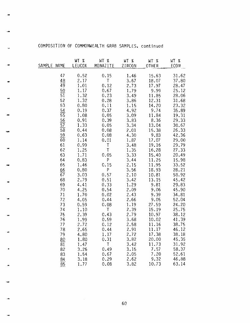
COMPOSITION OF COMMONWEALTH GRAB SAMPLES. continued

WT % WT % WT % WT % WT % - SAMPLE NAME LEUCOX MONAZITE ZIRCON OTHER ECON

47 0.52 0.15 1.46 15.63 31.62 48 2.17 T 3.67 18.07 37.80 49 1. 01 0.12 2.73 17.97 28.47 50 1.17 0.67 1. 79 9.99 25.12 51 1. 32 0.23 3.49 11.85 28.06 52 1.32 0.28 3.86 12.31 31.68 53 0.80 0.11 1.15 14.20 23.32 54 0.19 0.37 4.92 9.74 35.89

, ... 55 1. 08 0.05 3.09 11.84 19.31 56 0.91 0.39 3.83 8.36 29.33 57 1. 33 0.05 3.34 13.04 30.67

- 58 0.44 0.08 2.01 15.38 26.33 59 0.63 0.08 4.30 9.83 42.36 60 1.14 0.01 1.87 17.07 29.00 61 0.99 T 3.48 19.16 29.79 62 1. 25 T 1. 35 16.28 27.33 63 1.71 0.05 3.33 15.40 20.49 64 0.83 p 3.44 11.25 15.98 - 65 1.46 0.15 2.15 11.95 33.52 66 0.80 p 3.56 18.93 28.21 67 3.03 0.57 2.10 10.81 58.92

- 68 2.79 0.51 3.42 13.15 45.42 69 4.41 0.33 1.29 9.81 29.83 70 4.25 0.54 2.09 9.06 45.90 71 1. 70 0.02 2.43 9.39 34.81 72 4.05 0.44 2.66 9.05 52.04 73 0.59 0.08 1.19 27.59 24.20 74 1.10 T 2.39 15.19 25.75 75 2.39 0.43 2. 79 10.97 38.12 76 1.99 0.59 3.68 10.02 41.39 77 2.72 0.12 2.58 11.16 38.75 78 2.65 0.44 2.91 11.17 46.12 79 4.80 1.17 2.72 17.38 38.18 80 1.80 0.31 3.82 20.00 45.35 81 1.47 T 3.42 11.73 31.92 82 3.26 0.49 3.15 7. 57 58.37 83 1. 54 0.67 2.05 7.20 52.61 84 3.18 0.29 2.62 9.32 46.88 85 1.77 0.08 3.82 10.73 63.14

60

c. COMPOSITION OF COMMONWEALTH (USGS) CORE SAMPLES

WT% WT % WT % WT % WT % WT % SAMPLE NAME TOTAL HM MAG IL GAR EP STAUR

1090-1 2.46 8.30 26.15 14.81 9.05 0. 39 1090-2 1. 91 5.13 25.84 16.38 9.67 0.79 1091-1 2.36 3.67 24.11 15.31 8.10 0.52 1091-2 1.71 2.57 30.41 14.36 8.63 0.38 1091 3 1.61 6.14 37.86 10.46 6.19 0.90 1092-1 1. 70 0.85 45.28 9.81 13.01 1.48 ... 1092-2 1.03 0.76 46.82 3.69 14.91 1. 23 1094-1 1.15 3.24 36.10 13.20 7.20 1.13 1094-2 1.01 1.36 47.67 9.06 10.53 0.62 - 1095-1 2.51 10.29 23.13 18.31 6. 16 0.81 1095-2 2.30 1.15 46.39 4.67 16.89 2.29 1096-1 1.84 5.82 25.7 4 13.69 10.06 0. 77

,.,. 1096-2 2.23 2.83 39.03 8.67 18.06 1.25 1097-1 2.60 5.62 30.25 14.61 9.00 0.80 1097-2 1. 39 1.15 46.66 5.15 17.61 1.41 1097-3 1.26 1.25 53.25 8.56 4.52 0.76 1098-1 1. 78 0.75 49.89 5.39 15.01 2.63 1098-2 0.58 1.43 60.33 2.01 6.96 1. 34 1099-1 1.18 6.62 34.19 12.61 8.61 0.76

... 1099-2 1. 78 1.40 51.02 6.31 11.53 1.48 1100-1 2.64 10.58 24.72 13.15 5.16 0.58 1100-2 2.51 2.78 45.03 7.06 10.58 1.64 1103-1 1.80 2.55 38.64 14.57 6.16 0. 77 1103-2 1.62 1. 37 40.50 12.30 7.54 0.51 1103-3 1. 74 12.07 21.50 18.01 7.39 0.66 1106-1 3.59 3.78 37.70 22.82 7.69 0.05 1106-2 2.63 4.67 29.36 20.27 7.10 1.19 1107-1 4.35 4.00 30.76 17.18 6.55 1.03 1107 2 1.83 5.07 19.67 19.91 6.98 0.60 1109-1 3.08 7. 27 22.70 15.94 10.86 0.88 1111-1 2.76 12.52 24.43 17.48 6.26 0.13 1111-2 3.20 10.98 29.74 19.42 6.08 0.25 1116-1 4.39 13.45 25.36 15.21 5.66 0.46 1116-2 4.00 9.73 27.64 17.18 6.12 0.51 1119-1 2.43 4.89 21.87 20.14 7. 07 0.84 1119-2 2.39 6.97 28.19 19.36 4.85 0.34

... 1120-1 1.95 4.41 24.62 16.08 8.01 0.85

62

-

COMPOSITION OF COMMONWEALTH (USGS) CORE SAMPLES. continued

WT % WT % WT % WT % WT % WT % SAMPLE NAME AM PHI B PYROX RUTILE SILL/KY SPHENE TOURM

1090-1 13.82 9.35 0.94 0.31 0.23 0.32 - 1090-2 13.37 8.68 1. 23 1. 04 0.52 0. 57 1091-1 18.00 7.00 0. 56 . 0.81 0.88 0.73 1091-2 12.07 5.18 1.63 1. 02 0.32 0.09 1091-3 12.40 3.32 2.31 0.92 0.21 0.79 109 2-1 9.00 4.12 1.71 1. 61 0.00 0.16 1092-2 7.60 4.24 1. 93 1. 32 0.11 0.79 1094-1 14.83 5. 11 1. 26 0.60 0.44 0.65 1094-2 8.39 2.63 1.56 1.48 0.27 0.56 1095-1 14.39 6.22 0.68 0.46 0.39 0.61 1095-2 6.98 2.86 1.95 1.40 0.48 0.55

- 1096-1 21.12 4.99 0.36 0.98 0.26 0.66 1096-2 9.57 4.50 1.63 1. 27 0.16 0.18 1097-1 11.31 10.02 0.67 0.99 0.22 0.34 1097-2 9.00 1.96 1.23 1. 36 0.44 0.99 1097-3 10.76 3.46 2.12 0.82 0.28 0.45 1098-1 9.30 3.40 1. 34 2.25 0.45 0.05 1098-2 10.87 1. 56 1. 51 2.22 0.36 0.02 1099-1 13.75 3.94 1.52 0.63 0.30 0.67 1099-2 9.82 0.97 1.66 2.08 0.32 0.47 1100-1 18.46 8.98 0.66 0.93 0.65 0.33 1100-2 10.22 6.25 1. 25 1.85 0.10 0.09 1103-1 15.44 8.05 0.64 0.61 0.27 0.30 1103-2 12.49 4.85 1. 36 1.18 0.24 0.44 1103-3 13.60 8.92 1. 21 0.85 0.04 0.55 1106-1 11.86 4.36 0.81 0.68 0.28 0.32 1106-2 13.48 11.02 0.85 0.36 0.24 0.20 1107-1 14.89 9.64 0.66 0. 77 0.47 0.55 1107-2 22.10 9.55 1.43 0.75 0.49 0.35 1109-1 15.29 9.97 0.47 0.22 0.37 0.74 1111-1 15.17 7.75 1.19 0.46 0.23 0.23 1111-2 11.02 5.82 0.91 0.00 0.32 0.97 1116-1 16.48 5.25 0.96 0.50 0.62 0.11 1116-2 14.70 3.74 2.10 0.39 0.13 0.48 1119-1 22.89 4.70 1. 35 0.20 0.27 0.91 1119-2 17.10 5.43 1. 35 0.40 0.28 0.90 1120-1 19.70 8.00 1.09 0.98 0.13 1. 27 1120-2 10.63 6.09 1.05 0.23 0.17 0.06

64

-

COMPOSITION OF COMMONWEALTH (USGS) CORE SAMPLES. continued

WT % WT % WT % WT % WT % - SAMPLE NAME LEUCOX MONAZITE ZIRCON OTHER ECON

1090-1 0.44 T 3.05 12.85 30.89

'~·-1090-2 1. 33 0.07 3.69 11.68 33.20 1091-1 1.43 2.47 9.22 7.19 38.61 1091 2 1. 98 0.15 4.05 17.15 39.24 1091-3 1.16 T 4.64 12.70 46.89 .. 1092-1 1. 37 0.13 3.19 8.28 53.29 1092 2 3.15 0.05 4.90 8.50 58.18 1094-1 1. 33 0.01 2.93 11.98 42.23 - 1094-2 1. 71 0.01 4.19 9.96 56.62 109 5-1 1. 02 T 3.62 13.90 28.92 1095-2 1.47 p 3.26 9.67 54.46 1096-1 0.86 0.05 2.04 12.59 30.03 1096-2 1. 35 0.03 2.84 8.62 46.15 1097-1 1.08 T 4.42 10.68 37.40 1097-2 2.13 0.09 3.82 6.99 55.30 1097-3 1.95 T 3.17 8.65 61.31 1098-1 2.20 0.13 1.36 5.85 57.16 1098-2 2.01 0.16 3.08 6.14 69.30

""" 1099-1 2.10 0.01 4.21 10.08 42.66 1099-2 1. 31 0.25 3.00 8.38 59.32 1100-1 1.00 T 3.20 11.60 30.51 1100-2 0.83 0.01 3. 99 8. 31 52.97 1103-1 1.23 0.01 1.90 8.87 43.02 1103-2 3.12 T 2.74 11.35 48.90 1103-3 1.31 0.11 4.44 9.34 29.41 - 1106-1 0.77 0.09 2.32 6.48 42.37 1106-2 0.43 T 1. 70 9.14 32.69 1107-1 0.79 0.12 2.59 9.99 35.70

- 1107-2 1.17 0.19 2.01 9.74 25.22 1109-1 0.96 T 1.27 13.07 25.62 1111-1 0.82 0.03 3.88 9.42 30.81 1111-2 0.71 0.03 2. 72 11.03 34.11 - 2.69 12.40 30.36 1116-1 0. 75 0.10 1116-2 0.36 0.11 3.93 12.89 34.52 1119-1 0.93 0.22 2.17 11.53 26.75 1119-2 0.35 0.05 3.71 10.73 34.04 1120-1 0.55 0.23 2.08 11.99 29.55 1120-2 1.07 0.03 2.69 11.36 37.24

66

-- APPENDIX IV

SUMMARY COMPOSITION STATISTICS FOR ALL SAMPLES

WT% WT % WT % WT % WT % WT % TOTAL HM MAG IL GAR EP STAUR

average 3.46 5.54 27.83 15.45 7.03 1. 62 std. dev. 2.54 4. 77 10.86 5.39 3.27 1. 78 ,_ min value 0.14 0.07 7.65 2.01 0.47 0.00 max value 14.66 27.58 60.33 37.36 18.06 11.78

~-

WT % WT % WT % WT % WT % WT % AMPHIB PYROX RUTILE SILLIKY SPHENE TOURM -

average 15.52 6.20 1.16 1.12 0.45 0.58 std. dev. 6.23 3.41 0.55 0.91 0.36 0.51

- min value 0.00 0.41 0.00 0.00 0.00 0.00 max value 34.71 21.82 3.15 5.19 2.04 3.94

... WT % WT % WT % WT % WT %

LEUCOX MONAZITE ZIRCON OTHER ECON - average 1.41 0.22 3.01 12.87 34.74 std. dev. 0.92 0.33 1. 22 5.48 12.01 min va 1 ue 0.00 0.00 0.62 3.52 13.61 max value 5. 39 2.47 9.22 37.73 69.30

...

-

-

68

APPENDIX V. continued

·- wt% IL wt% RUT wt% LEUCX wt% MON wt% ZR wt% ECON SAMPLE NAME of TOTAL of TOTAL of TOTAL of TOTAL of TOTAL of TOTAL

V1 1 0.23 0.02 0.01 0.00 0.04 0.30 V1-2 0.42 0.02 0.02 0.00 0.02 0.49 V1-3 0.28 0.01 0.01 0.00 0.02 0.34 - V1-4 0.46 0.01 0.03 0.00 0.03 0.55 V2-1 0.65 0.02 0.03 0.00 0.06 0.81 V2-2 0.76 0.04 0.03 0.00 0.10 0.94 V2-3 1.45 0.05 0.07 0.01 0.12 1.84 V2-4 1.06 0.03 0.03 0.00 0.08 1.23 V4-1 0.42 0.01 0.03 0.00 0.05 0.53 V4-2 0.41 0.02 0.02 0.00 0.02 0.49 ·- V4-3 0.45 0.02 0.04 0.00 0.03 o. 57 V4-4 0.61 0.03 0.04 0.00 0.04 0.74 V3-1 0.46 0.02 0.08 0.00 0.05 0.64

.... V3-2 0.18 0.01 0.01 0.00 0.02 0.23 V5-1 0.35 0.02 0.03 0.00 0.08 0.50 V5-3 0.54 0.02 0.03 0.00 0.05 0.67 V5-4 0.53 0.02 0.02 0.00 0.06 0.65 V5-5 0.66 0.02 0.05 0.00 0.06 0.82 V6-1 0.60 0.03 0.01 0.00 0.11 0.76 V6-2 0.43 0.03 0.01 0.00 0.11 0.58

1 1.22 0.02 0.03 0.00 0.11 1. 41 2 1.94 0.05 0.06 0.03 0.16 2.31 3 1.01 0.04 0.05 0.00 0. 07 1.19

- 1. 1.99 0.13 0.28 0.02 0.31 2.86 §. 1.84 0.07 0.13 0.01 0.32 2.38 6 0.52 0.01 0.03 0.01 0.03 0.62 7 0.40 0.01 0.02 0.00 0.06 0.50 - 8 0.58 0.01 0.03 0.01 0.04 0.67 9 0.44 0.01 0.02 0.00 0.03 0.52

10 1. 93 0.03 0.07 0.01 0.05 2.09 IT 0.48 0.02 0.03 0.03 0.04 0.60 12 2.03 0.07 0.13 0.00 0.26 2.51 13 0.61 0.02 0.03 0.01 0.06 0.73 14 1.58 0.05 0.16 0.05 0.09 2.03 15 2.08 0.08 0.08 0.01 0.32 2.65 22 1.08 0.02 0.14 0.03 0.08 1. 38 23 0.43 0.03 0.02 0.00 0.05 0.55 24 0.73 0.03 0.08 0.01 0.08 0.98 25 1.00 0.06 0.10 0.02 0.10 1. 30 27 0.13 0.01 0.01 0.00 0.02 0.19 28 0.83 0.01 0.03 0.01 0.05 0.94 29 0.64 0.05 0.03 T 0.11 0.87

70

·-

APPENDIX V. continued

wt% IL wt% RUT wt% LEUCX wt% MON wt% ZR wt% ECON SAMPLE NAME of TOTAL of TOTAL of TOTAL of TOTAL of TOTAL of TOTAL

- 74 0.93 0.05 0.05 T 0.11 1.13 75 0.16 0.01 0.01 0.00 0.02 0.21 76 0.15 0.01 0.01 0.00 0.02 0.20 77 0.47 0.02 0.04 0.00 0.04 0.59 78 0.39 0.02 0.03 0.00 0.03 0.48 79 0.03 0.00 0.01 0.00 0.00 0.05 80 1. 81 0.04 0.09 0.01 0.18 2.15 81 1.08 0.07 0.06 T 0.15 1.40 82 0.62 0.04 0.04 0.01 0.04 0.76 83 0.31 0.02 0.01 0.00 0.01 0.37 - 84 0.19 0.01 0.02 0.00 0.01 0.24 85 5.90 0.26 0.19 0.01 0.41 6.79 86 0.43 0.03 0.04 0.00 0.04 0.55 - 87 1. 78 0.10 0.10 0.01 0.14 2.16 88 0.14 0.01 0.02 0.00 0.01 0. 19 89 1.01 0.07 0.11 0.01 0.15 1.36 .. 89A 2.06 0.08 0.08 0.01 0.11 2.37 90 0.34 0.01 0.03 0.01 0.03 0.42 91 2.24 0.04 0.12 0.01 0.15 2.61 93 0.29 0.01 0.03 0.01 0.03 0.38 ·- 94 0.29 0.02 0.02 0.00 0.01 0.36 95 0.08 0.00 0.01 0.00 0.01 0.12 96 0.34 0.01 0.01 0.01 0.03 0.43

·- 97 0.44 0.02 0.02 0.00 0.03 0.52 98 2.59 0.11 0.12 0.04 0.22 3.18

100 1.88 0.09 0.04 0.00 0.16 2.22 101 0.82 0.03 0.04 0.00 0.07 0.98

1090-1 0.64 0.02 0.01 T 0.08 0.76 1090-2 0.49 0.02 0.03 0.00 0.07 0.63 1091-1 0.57 0.01 0.03 0.06 0.22 0.91 1091-2 0.52 0.03 0.03 0.00 0.07 0.67 1091-3 0.61 0.04 0.02 T 0.07 0.75 1092-1 0.77 0.03 0.02 0.00 0.05 0.90

·- 1092-2 0.48 0.02 0.03 0.00 0.05 0.60 1094-1 0.42 0.01 0.02 0.00 0.03 0.49 1094-2 0.48 0.02 0.02 0.00 0.04 0. 57 1095-1 0.58 0.02 0.03 T 0.09 0.72 1095-2 1.07 0.04 0.03 p 0.07 1.25 1096-1 0.47 0.01 0.02 0.00 0.04 0.55 1096-2 0.87 0.04 0.03 0.00 0.06 1.03 1097-1 0.79 0.02 0.03 T 0.11 0.97 1097-2 0.65 0.02 0.03 0.00 0.05 0.77

72

-

APPENDIX V. continued

wt% IL wt% RUT wt% LEUCX wt% MON wt% ZR wt% ECON SAMPLE NAME of TOTAL of TOTAL of TOTAL of TOTAL of TOTAL of TOTAL

··- 2001-1 0.41 0.02 0.04 0.00 0.04 0.52 2002-1 1.09 0.02 0.01 p 0.12 1.25 2002-2 0.89 0.01 0.03 0.00 0.07 1. 01 .... 110-1 0.84 0.04 0.01 T 0.14 1.06 110-2 0.41 0.03 0.02 T 0.05 0.53 110-3 0.29 0.02 0.02 0.00 0.02 0.36 115 1 0.21 0.01 0.01 0.00 0.02 0.25 116-1 0.18 0.01 0.01 0.00 0.02 0.24 116-2 0.17 0.01 0.01 0.00 0.01 0.22 .. 116-3 0. 78 0.03 0.04 T 0.08 0.97 116-4 0.33 0.02 0.01 0.00 0.04 0.42 116-5 0.52 0.05 0.04 0.00 0.05 0.70 117-1 0.38 0.02 0.02 0.00 0.03 0.46 117-2 1.07 0.07 0.04 0.00 0.08 1.33 117-3 1.12 0.04 0.04 0.01 0.07 1. 33 117-4 0.65 0.04 0.04 0.00 0.05 0.82

average 0.92 0.04 0.04 0.01 0.10 1.14 std. dev. 0.79 0.03 0.04 0.01 0.10 0.94 min value 0.03 0.00 0.00 0.00 0.00 0.05 max value 5.90 0.26 0.28 0.08 0. 72 6.79

.. Garner's values 2.25 0.10 0.25 0.05 0.25 (see text)

-

74