Vijay V. Vazirani

College of ComputingGeorgia Institute of Technology

Copyright c© 2001

Approximation Algorithms

SpringerBerlin Heidelberg NewYorkBarcelona Hong KongLondon Milan ParisSingapore Tokyo

To my parents

Preface

Although this may seem a paradox, all exactscience is dominated by the idea of approximation.

Bertrand Russell (1872–1970)

Most natural optimization problems, including those arising in importantapplication areas, are NP-hard. Therefore, under the widely believed con-jecture that P �= NP, their exact solution is prohibitively time consuming.Charting the landscape of approximability of these problems, via polynomialtime algorithms, therefore becomes a compelling subject of scientific inquiryin computer science and mathematics. This book presents the theory of ap-proximation algorithms as it stands today. It is reasonable to expect thepicture to change with time.

The book is divided into three parts. In Part I we cover a combinato-rial algorithms for a number of important problems, using a wide varietyof algorithm design techniques. The latter may give Part I a non-cohesiveappearance. However, this is to be expected – nature is very rich, and wecannot expect a few tricks to help solve the diverse collection of NP-hardproblems. Indeed, in this part, we have purposely refrained from tightly cat-egorizing algorithmic techniques so as not to trivialize matters. Instead, wehave attempted to capture, as accurately as possible, the individual characterof each problem, and point out connections between problems and algorithmsfor solving them.

In Part II, we present linear programming based algorithms. These arecategorized under two fundamental techniques: rounding and the primal–dual schema. But once again, the exact approximation guarantee obtainabledepends on the specific LP-relaxation used, and there is no fixed recipe fordiscovering good relaxations, just as there is no fixed recipe for proving a the-orem in mathematics (readers familiar with complexity theory will recognizethis as the philosophical point behind the P �= NP question).

Part III covers four important topics. The first is the problem of findinga shortest vector in a lattice which, for several reasons, deserves individualtreatment (see Chapter 27).

The second topic is the approximability of counting, as opposed tooptimization, problems (counting the number of solutions to a given in-stance). The counting versions of all known NP-complete problems are #P-complete1. Interestingly enough, other than a handful of exceptions, this istrue of problems in P as well. An impressive theory has been built for ob-1 However, there is no theorem to this effect yet.

VIII Preface

taining efficient approximate counting algorithms for this latter class of prob-lems. Most of these algorithms are based on the Markov chain Monte Carlo(MCMC) method, a topic that deserves a book by itself and is therefore nottreated here. In Chapter 28 we present combinatorial algorithms, not usingthe MCMC method, for two fundamental counting problems.

The third topic is centered around recent breakthrough results, estab-lishing hardness of approximation for many key problems, and giving newlegitimacy to approximation algorithms as a deep theory. An overview ofthese results is presented in Chapter 29, assuming the main technical theo-rem, the PCP Theorem. The latter theorem, unfortunately, does not have asimple proof at present.

The fourth topic consists of the numerous open problems of this youngfield. The list presented should by no means be considered exhaustive, andis moreover centered around problems and issues currently in vogue. Exactalgorithms have been studied intensively for over four decades, and yet basicinsights are still being obtained. Considering the fact that among naturalcomputational problems, polynomial time solvability is the exception ratherthan the rule, it is only reasonable to expect the theory of approximationalgorithms to grow considerably over the years.

The set cover problem occupies a special place, not only in the theory ofapproximation algorithms, but also in this book. It offers a particularly simplesetting for introducing key concepts as well as some of the basic algorithmdesign techniques of Part I and Part II. In order to give a complete treatmentfor this central problem, in Part III we give a hardness result for it, eventhough the proof is quite elaborate. The hardness result essentially matchesthe guarantee of the best algorithm known – this being another reason forpresenting this rather difficult proof.

Our philosophy on the design and exposition of algorithms is nicely il-lustrated by the following analogy with an aspect of Michelangelo’s art. Amajor part of his effort involved looking for interesting pieces of stone in thequarry and staring at them for long hours to determine the form they natu-rally wanted to take. The chisel work exposed, in a minimalistic manner, thisform. By analogy, we would like to start with a clean, simply stated problem(perhaps a simplified version of the problem we actually want to solve inpractice). Most of the algorithm design effort actually goes into understand-ing the algorithmically relevant combinatorial structure of the problem. Thealgorithm exploits this structure in a minimalistic manner. The exposition ofalgorithms in this book will also follow this analogy, with emphasis on statingthe structure offered by problems, and keeping the algorithms minimalistic.

An attempt has been made to keep individual chapters short and simple,often presenting only the key result. Generalizations and related results arerelegated to exercises. The exercises also cover other important results whichcould not be covered in detail due to logistic constraints. Hints have been

Preface IX

provided for some of the exercises; however, there is no correlation betweenthe degree of difficulty of an exercise and whether a hint is provided for it.

This book is suitable for use in advanced undergraduate and graduate levelcourses on approximation algorithms. It has more than twice the materialthat can be covered in a semester long course, thereby leaving plenty of roomfor an instructor to choose topics. An undergraduate course in algorithmsand the theory of NP-completeness should suffice as a prerequisite for mostof the chapters. For completeness, we have provided background informationon several topics: complexity theory in Appendix A, probability theory inAppendix B, linear programming in Chapter 12, semidefinite programming inChapter 26, and lattices in Chapter 27. (A disproportionate amount of spacehas been devoted to the notion of self-reducibility in Appendix A becausethis notion has been quite sparsely treated in other sources.) This book canalso be used is as supplementary text in basic undergraduate and graduatealgorithms courses. The first few chapters of Part I and Part II are suitablefor this purpose. The ordering of chapters in both these parts is roughly byincreasing difficulty.

In anticipation of this wide audience, we decided not to publish this bookin any of Springer’s series – even its prestigious Yellow Series. (However, wecould not resist spattering a patch of yellow on the cover!) The followingtranslations are currently planned: French by Claire Kenyon, Japanese byTakao Asano, and Romanian by Ion Mandoiu. Corrections and commentsfrom readers are welcome. We have set up a special email address for thispurpose: approx@cc.gatech.edu.

Finally, a word about practical impact. With practitioners looking forhigh performance algorithms having error within 2% or 5% of the optimal,what good are algorithms that come within a factor of 2, or even worse,O(log n), of the optimal? Further, by this token, what is the usefulness ofimproving the approximation guarantee from, say, factor 2 to 3/2?

Let us address both issues and point out some fallacies in these assertions.The approximation guarantee only reflects the performance of the algorithmon the most pathological instances. Perhaps it is more appropriate to viewthe approximation guarantee as a measure that forces us to explore deeperinto the combinatorial structure of the problem and discover more powerfultools for exploiting this structure. It has been observed that the difficultyof constructing tight examples increases considerably as one obtains algo-rithms with better guarantees. Indeed, for some recent algorithms, obtaininga tight example has been a paper by itself (e.g., see Section 26.7). Experi-ments have confirmed that these and other sophisticated algorithms do haveerror bounds of the desired magnitude, 2% to 5%, on typical instances, eventhough their worst case error bounds are much higher. Additionally, the the-oretically proven algorithm should be viewed as a core algorithmic idea thatneeds to be fine tuned to the types of instances arising in specific applications.

X Preface

We hope that this book will serve as a catalyst in helping this theory growand have practical impact.

Acknowledgments

This book is based on courses taught at the Indian Institute of Technology,Delhi in Spring 1992 and Spring 1993, at Georgia Tech in Spring 1997, Spring1999, and Spring 2000, and at DIMACS in Fall 1998. The Spring 1992 courseresulted in the first set of class notes on this topic. It is interesting to notethat more than half of this book is based on subsequent research results.

Numerous friends – and family members – have helped make this book areality. First, I would like to thank Naveen Garg, Kamal Jain, Ion Mandoiu,Sridhar Rajagopalan, Huzur Saran, and Mihalis Yannakakis – my extensivecollaborations with them helped shape many of the ideas presented in thisbook. I was fortunate to get Ion Mandoiu’s help and advice on numerousmatters – his elegant eye for layout and figures helped shape the presentation.A special thanks, Ion!

I would like to express my gratitude to numerous experts in the field forgenerous help on tasks ranging all the way from deciding the contents andits organization, providing feedback on the writeup, ensuring correctness andcompleteness of references to designing exercises and helping list open prob-lems. Thanks to Sanjeev Arora, Alan Frieze, Naveen Garg, Michel Goemans,Mark Jerrum, Claire Kenyon, Samir Khuller, Daniele Micciancio, Yuval Ra-bani, Sridhar Rajagopalan, Dana Randall, Tim Roughgarden, Amin Saberi,Leonard Schulman, Amin Shokrollahi, and Mihalis Yannakakis, with specialthanks to Kamal Jain, Eva Tardos, and Luca Trevisan.

Numerous other people helped with valuable comments and discussions.In particular, I would like to thank Sarmad Abbasi, Cristina Bazgan, RogerioBrito Gruia Calinescu, Amit Chakrabarti, Mosses Charikar, Joseph Cheriyan,Vasek Chvatal, Uri Feige, Cristina Fernandes, Ashish Goel, Parikshit Gopalan,Mike Grigoriadis, Sudipto Guha, Dorit Hochbaum, Howard Karloff, LeonidKhachian, Stavros Kolliopoulos, Jan van Leeuwen, Nati Lenial, GeorgeLeuker, Vangelis Markakis, Aranyak Mehta, Rajeev Motwani, PrabhakarRaghavan, Satish Rao, Miklos Santha, Jiri Sgall, David Shmoys, AlistairSinclair, Prasad Tetali, Pete Veinott, Ramarathnam Venkatesan, NisheethVishnoi, and David Williamson. I am sure I am missing several names – myapologies and thanks to these people as well. A special role was played bythe numerous students who took my courses on this topic and scribed notes.It will be impossible to individually remember their names. I would like toexpress my gratitude collectively to them.

I would like to thank IIT Delhi – with special thanks to Shachin Mahesh-wari – Georgia Tech, and DIMACS for providing pleasant, supportive andacademically rich environments. Thanks to NSF for support under grantsCCR-9627308 and CCR-9820896.

Preface XI

It was a pleasure to work with Hans Wossner on editorial matters. Thepersonal care with which he handled all such matters and his sensitivity toan author’s unique point of view were especially impressive. Thanks also toFrank Holzwarth for sharing his expertise with LATEX.

A project of this magnitude would be hard to pull off without whole-hearted support from family members. Fortunately, in my case, some of themare also fellow researchers – my wife, Milena Mihail, and my brother, UmeshVazirani. Little Michel’s arrival, halfway through this project, brought newjoys and energies, though made the end even more challenging! Above all,I would like to thank my parents for their unwavering support and inspira-tion – my father, a distinguished author of several Civil Engineering books,and my mother, with her deep understanding of Indian Classical Music. Thisbook is dedicated to them.

Atlanta, Georgia, May 2001 Vijay Vazirani

Table of Contents

1 Introduction . . . . . . . . . . . . . . . . . . . . . . . . . . . . . . . . . . . . . . . . . . . . . . 11.1 Lower bounding OPT . . . . . . . . . . . . . . . . . . . . . . . . . . . . . . . . . . . 2

1.1.1 An approximation algorithm for cardinality vertex cover 31.1.2 Can the approximation guarantee be improved? . . . . . . 3

1.2 Well-characterized problems and min–max relations . . . . . . . . . 51.3 Exercises . . . . . . . . . . . . . . . . . . . . . . . . . . . . . . . . . . . . . . . . . . . . . . 71.4 Notes . . . . . . . . . . . . . . . . . . . . . . . . . . . . . . . . . . . . . . . . . . . . . . . . . 10

Part I. Combinatorial Algorithms

2 Set Cover . . . . . . . . . . . . . . . . . . . . . . . . . . . . . . . . . . . . . . . . . . . . . . . . . 152.1 The greedy algorithm . . . . . . . . . . . . . . . . . . . . . . . . . . . . . . . . . . . 162.2 Layering . . . . . . . . . . . . . . . . . . . . . . . . . . . . . . . . . . . . . . . . . . . . . . 172.3 Application to shortest superstring . . . . . . . . . . . . . . . . . . . . . . . 192.4 Exercises . . . . . . . . . . . . . . . . . . . . . . . . . . . . . . . . . . . . . . . . . . . . . . 222.5 Notes . . . . . . . . . . . . . . . . . . . . . . . . . . . . . . . . . . . . . . . . . . . . . . . . . 26

3 Steiner Tree and TSP . . . . . . . . . . . . . . . . . . . . . . . . . . . . . . . . . . . . 273.1 Metric Steiner tree . . . . . . . . . . . . . . . . . . . . . . . . . . . . . . . . . . . . . 27

3.1.1 MST-based algorithm . . . . . . . . . . . . . . . . . . . . . . . . . . . . . 283.2 Metric TSP . . . . . . . . . . . . . . . . . . . . . . . . . . . . . . . . . . . . . . . . . . . . 30

3.2.1 A simple factor 2 algorithm . . . . . . . . . . . . . . . . . . . . . . . . 313.2.2 Improving the factor to 3/2 . . . . . . . . . . . . . . . . . . . . . . . . 32

3.3 Exercises . . . . . . . . . . . . . . . . . . . . . . . . . . . . . . . . . . . . . . . . . . . . . . 333.4 Notes . . . . . . . . . . . . . . . . . . . . . . . . . . . . . . . . . . . . . . . . . . . . . . . . . 37

4 Multiway Cut and k-Cut . . . . . . . . . . . . . . . . . . . . . . . . . . . . . . . . . 384.1 The multiway cut problem . . . . . . . . . . . . . . . . . . . . . . . . . . . . . . . 384.2 The minimum k-cut problem . . . . . . . . . . . . . . . . . . . . . . . . . . . . . 404.3 Exercises . . . . . . . . . . . . . . . . . . . . . . . . . . . . . . . . . . . . . . . . . . . . . . 444.4 Notes . . . . . . . . . . . . . . . . . . . . . . . . . . . . . . . . . . . . . . . . . . . . . . . . . 46

XIV Table of Contents

5 k-Center . . . . . . . . . . . . . . . . . . . . . . . . . . . . . . . . . . . . . . . . . . . . . . . . . . 475.1 Parametric pruning applied to metric k-center . . . . . . . . . . . . . . 475.2 The weighted version . . . . . . . . . . . . . . . . . . . . . . . . . . . . . . . . . . . 505.3 Exercises . . . . . . . . . . . . . . . . . . . . . . . . . . . . . . . . . . . . . . . . . . . . . . 525.4 Notes . . . . . . . . . . . . . . . . . . . . . . . . . . . . . . . . . . . . . . . . . . . . . . . . . 53

6 Feedback Vertex Set . . . . . . . . . . . . . . . . . . . . . . . . . . . . . . . . . . . . . . 546.1 Cyclomatic weighted graphs . . . . . . . . . . . . . . . . . . . . . . . . . . . . . 546.2 Layering applied to feedback vertex set . . . . . . . . . . . . . . . . . . . . 576.3 Exercises . . . . . . . . . . . . . . . . . . . . . . . . . . . . . . . . . . . . . . . . . . . . . . 606.4 Notes . . . . . . . . . . . . . . . . . . . . . . . . . . . . . . . . . . . . . . . . . . . . . . . . . 60

7 Shortest Superstring . . . . . . . . . . . . . . . . . . . . . . . . . . . . . . . . . . . . . . 617.1 A factor 4 algorithm . . . . . . . . . . . . . . . . . . . . . . . . . . . . . . . . . . . . 617.2 Improving to factor 3 . . . . . . . . . . . . . . . . . . . . . . . . . . . . . . . . . . . 64

7.2.1 Achieving half the optimal compression . . . . . . . . . . . . . 667.3 Exercises . . . . . . . . . . . . . . . . . . . . . . . . . . . . . . . . . . . . . . . . . . . . . . 667.4 Notes . . . . . . . . . . . . . . . . . . . . . . . . . . . . . . . . . . . . . . . . . . . . . . . . . 67

8 Knapsack . . . . . . . . . . . . . . . . . . . . . . . . . . . . . . . . . . . . . . . . . . . . . . . . . 688.1 A pseudo-polynomial time algorithm for knapsack . . . . . . . . . . 698.2 An FPTAS for knapsack . . . . . . . . . . . . . . . . . . . . . . . . . . . . . . . . 698.3 Strong NP-hardness and the existence of FPTAS’s . . . . . . . . . 71

8.3.1 Is an FPTAS the most desirable approximationalgorithm?. . . . . . . . . . . . . . . . . . . . . . . . . . . . . . . . . . . . . . . 72

8.4 Exercises . . . . . . . . . . . . . . . . . . . . . . . . . . . . . . . . . . . . . . . . . . . . . . 728.5 Notes . . . . . . . . . . . . . . . . . . . . . . . . . . . . . . . . . . . . . . . . . . . . . . . . . 73

9 Bin Packing . . . . . . . . . . . . . . . . . . . . . . . . . . . . . . . . . . . . . . . . . . . . . . 749.1 An asymptotic PTAS . . . . . . . . . . . . . . . . . . . . . . . . . . . . . . . . . . . 749.2 Exercises . . . . . . . . . . . . . . . . . . . . . . . . . . . . . . . . . . . . . . . . . . . . . . 779.3 Notes . . . . . . . . . . . . . . . . . . . . . . . . . . . . . . . . . . . . . . . . . . . . . . . . . 78

10 Minimum Makespan Scheduling . . . . . . . . . . . . . . . . . . . . . . . . . . 7910.1 Factor 2 algorithm . . . . . . . . . . . . . . . . . . . . . . . . . . . . . . . . . . . . . . 7910.2 A PTAS for minimum makespan . . . . . . . . . . . . . . . . . . . . . . . . . 80

10.2.1 Bin packing with fixed number of object sizes . . . . . . . . 8110.2.2 Reducing makespan to restricted bin packing . . . . . . . . 81

10.3 Exercises . . . . . . . . . . . . . . . . . . . . . . . . . . . . . . . . . . . . . . . . . . . . . . 8310.4 Notes . . . . . . . . . . . . . . . . . . . . . . . . . . . . . . . . . . . . . . . . . . . . . . . . . 83

11 Euclidean TSP . . . . . . . . . . . . . . . . . . . . . . . . . . . . . . . . . . . . . . . . . . . 8411.1 The algorithm . . . . . . . . . . . . . . . . . . . . . . . . . . . . . . . . . . . . . . . . . 8411.2 Proof of correctness . . . . . . . . . . . . . . . . . . . . . . . . . . . . . . . . . . . . . 8711.3 Exercises . . . . . . . . . . . . . . . . . . . . . . . . . . . . . . . . . . . . . . . . . . . . . . 8911.4 Notes . . . . . . . . . . . . . . . . . . . . . . . . . . . . . . . . . . . . . . . . . . . . . . . . . 89

Table of Contents XV

Part II. LP-Based Algorithms

12 Introduction to LP-Duality . . . . . . . . . . . . . . . . . . . . . . . . . . . . . . . 9312.1 The LP-duality theorem . . . . . . . . . . . . . . . . . . . . . . . . . . . . . . . . . 9312.2 Min–max relations and LP-duality . . . . . . . . . . . . . . . . . . . . . . . . 9712.3 Two fundamental algorithm design techniques . . . . . . . . . . . . . . 100

12.3.1 A comparison of the techniques and the notion ofintegrality gap . . . . . . . . . . . . . . . . . . . . . . . . . . . . . . . . . . . 101

12.4 Exercises . . . . . . . . . . . . . . . . . . . . . . . . . . . . . . . . . . . . . . . . . . . . . . 10312.5 Notes . . . . . . . . . . . . . . . . . . . . . . . . . . . . . . . . . . . . . . . . . . . . . . . . . 107

13 Set Cover via Dual Fitting . . . . . . . . . . . . . . . . . . . . . . . . . . . . . . . . 10813.1 Dual-fitting-based analysis for the greedy set cover algorithm 108

13.1.1 Can the approximation guarantee be improved? . . . . . . 11113.2 Generalizations of set cover . . . . . . . . . . . . . . . . . . . . . . . . . . . . . . 112

13.2.1 Dual fitting applied to constrained set multicover . . . . . 11213.3 Exercises . . . . . . . . . . . . . . . . . . . . . . . . . . . . . . . . . . . . . . . . . . . . . . 11613.4 Notes . . . . . . . . . . . . . . . . . . . . . . . . . . . . . . . . . . . . . . . . . . . . . . . . . 118

14 Rounding Applied to Set Cover . . . . . . . . . . . . . . . . . . . . . . . . . . . 11914.1 A simple rounding algorithm . . . . . . . . . . . . . . . . . . . . . . . . . . . . . 11914.2 Randomized rounding . . . . . . . . . . . . . . . . . . . . . . . . . . . . . . . . . . . 12014.3 Half-integrality of vertex cover . . . . . . . . . . . . . . . . . . . . . . . . . . . 12214.4 Exercises . . . . . . . . . . . . . . . . . . . . . . . . . . . . . . . . . . . . . . . . . . . . . . 12314.5 Notes . . . . . . . . . . . . . . . . . . . . . . . . . . . . . . . . . . . . . . . . . . . . . . . . . 124

15 Set Cover via the Primal–Dual Schema . . . . . . . . . . . . . . . . . . . 12515.1 Overview of the schema . . . . . . . . . . . . . . . . . . . . . . . . . . . . . . . . . 12515.2 Primal–dual schema applied to set cover . . . . . . . . . . . . . . . . . . . 12715.3 Exercises . . . . . . . . . . . . . . . . . . . . . . . . . . . . . . . . . . . . . . . . . . . . . . 12915.4 Notes . . . . . . . . . . . . . . . . . . . . . . . . . . . . . . . . . . . . . . . . . . . . . . . . . 129

16 Maximum Satisfiability . . . . . . . . . . . . . . . . . . . . . . . . . . . . . . . . . . . 13116.1 Dealing with large clauses . . . . . . . . . . . . . . . . . . . . . . . . . . . . . . . 13216.2 Derandomizing via the method of conditional expectation . . . 13216.3 Dealing with small clauses via LP-rounding . . . . . . . . . . . . . . . . 13416.4 A 3/4 factor algorithm . . . . . . . . . . . . . . . . . . . . . . . . . . . . . . . . . . 13616.5 Exercises . . . . . . . . . . . . . . . . . . . . . . . . . . . . . . . . . . . . . . . . . . . . . . 13716.6 Notes . . . . . . . . . . . . . . . . . . . . . . . . . . . . . . . . . . . . . . . . . . . . . . . . . 139

17 Scheduling on Unrelated Parallel Machines . . . . . . . . . . . . . . . 14017.1 Parametric pruning in an LP setting . . . . . . . . . . . . . . . . . . . . . . 14017.2 Properties of extreme point solutions . . . . . . . . . . . . . . . . . . . . . . 14117.3 The algorithm . . . . . . . . . . . . . . . . . . . . . . . . . . . . . . . . . . . . . . . . . 142

XVI Table of Contents

17.4 Additional properties of extreme point solutions . . . . . . . . . . . . 14317.5 Exercises . . . . . . . . . . . . . . . . . . . . . . . . . . . . . . . . . . . . . . . . . . . . . . 14417.6 Notes . . . . . . . . . . . . . . . . . . . . . . . . . . . . . . . . . . . . . . . . . . . . . . . . . 145

18 Multicut and Integer Multicommodity Flow in Trees . . . . . 14618.1 The problems and their LP-relaxations . . . . . . . . . . . . . . . . . . . . 14618.2 Primal–dual schema based algorithm . . . . . . . . . . . . . . . . . . . . . . 14918.3 Exercises . . . . . . . . . . . . . . . . . . . . . . . . . . . . . . . . . . . . . . . . . . . . . . 15218.4 Notes . . . . . . . . . . . . . . . . . . . . . . . . . . . . . . . . . . . . . . . . . . . . . . . . . 154

19 Multiway Cut . . . . . . . . . . . . . . . . . . . . . . . . . . . . . . . . . . . . . . . . . . . . 15519.1 An interesting LP-relaxation . . . . . . . . . . . . . . . . . . . . . . . . . . . . . 15519.2 Randomized rounding algorithm . . . . . . . . . . . . . . . . . . . . . . . . . . 15719.3 Half-integrality of node multiway cut . . . . . . . . . . . . . . . . . . . . . 16019.4 Exercises . . . . . . . . . . . . . . . . . . . . . . . . . . . . . . . . . . . . . . . . . . . . . . 16319.5 Notes . . . . . . . . . . . . . . . . . . . . . . . . . . . . . . . . . . . . . . . . . . . . . . . . . 167

20 Multicut in General Graphs . . . . . . . . . . . . . . . . . . . . . . . . . . . . . . 16820.1 Sum multicommodity flow . . . . . . . . . . . . . . . . . . . . . . . . . . . . . . . 16820.2 LP-rounding-based algorithm . . . . . . . . . . . . . . . . . . . . . . . . . . . . 170

20.2.1 Growing a region: the continuous process . . . . . . . . . . . . 17120.2.2 The discrete process . . . . . . . . . . . . . . . . . . . . . . . . . . . . . . 17220.2.3 Finding successive regions . . . . . . . . . . . . . . . . . . . . . . . . . 173

20.3 A tight example . . . . . . . . . . . . . . . . . . . . . . . . . . . . . . . . . . . . . . . . 17520.4 Some applications of multicut . . . . . . . . . . . . . . . . . . . . . . . . . . . . 17620.5 Exercises . . . . . . . . . . . . . . . . . . . . . . . . . . . . . . . . . . . . . . . . . . . . . . 17720.6 Notes . . . . . . . . . . . . . . . . . . . . . . . . . . . . . . . . . . . . . . . . . . . . . . . . . 179

21 Sparsest Cut . . . . . . . . . . . . . . . . . . . . . . . . . . . . . . . . . . . . . . . . . . . . . . 18021.1 Demands multicommodity flow . . . . . . . . . . . . . . . . . . . . . . . . . . . 18021.2 Linear programming formulation . . . . . . . . . . . . . . . . . . . . . . . . . 18121.3 Metrics, cut packings, and �1-embeddability . . . . . . . . . . . . . . . . 183

21.3.1 Cut packings for metrics . . . . . . . . . . . . . . . . . . . . . . . . . . 18321.3.2 �1-embeddability of metrics . . . . . . . . . . . . . . . . . . . . . . . . 185

21.4 Low distortion �1-embeddings for metrics . . . . . . . . . . . . . . . . . . 18621.4.1 Ensuring that a single edge is not overshrunk . . . . . . . . 18721.4.2 Ensuring that no edge is overshrunk . . . . . . . . . . . . . . . . 190

21.5 LP-rounding-based algorithm . . . . . . . . . . . . . . . . . . . . . . . . . . . . 19121.6 Applications . . . . . . . . . . . . . . . . . . . . . . . . . . . . . . . . . . . . . . . . . . . 192

21.6.1 Edge expansion . . . . . . . . . . . . . . . . . . . . . . . . . . . . . . . . . . 19221.6.2 Conductance . . . . . . . . . . . . . . . . . . . . . . . . . . . . . . . . . . . . . 19221.6.3 Balanced cut . . . . . . . . . . . . . . . . . . . . . . . . . . . . . . . . . . . . 19321.6.4 Minimum cut linear arrangement . . . . . . . . . . . . . . . . . . . 194

21.7 Exercises . . . . . . . . . . . . . . . . . . . . . . . . . . . . . . . . . . . . . . . . . . . . . . 19521.8 Notes . . . . . . . . . . . . . . . . . . . . . . . . . . . . . . . . . . . . . . . . . . . . . . . . . 197

Table of Contents XVII

22 Steiner Forest . . . . . . . . . . . . . . . . . . . . . . . . . . . . . . . . . . . . . . . . . . . . 19822.1 LP-relaxation and dual . . . . . . . . . . . . . . . . . . . . . . . . . . . . . . . . . . 19822.2 Primal–dual schema with synchronization . . . . . . . . . . . . . . . . . 19922.3 Analysis . . . . . . . . . . . . . . . . . . . . . . . . . . . . . . . . . . . . . . . . . . . . . . . 20422.4 Exercises . . . . . . . . . . . . . . . . . . . . . . . . . . . . . . . . . . . . . . . . . . . . . . 20722.5 Notes . . . . . . . . . . . . . . . . . . . . . . . . . . . . . . . . . . . . . . . . . . . . . . . . . 212

23 Steiner Network . . . . . . . . . . . . . . . . . . . . . . . . . . . . . . . . . . . . . . . . . . 21323.1 The LP-relaxation and half-integrality . . . . . . . . . . . . . . . . . . . . 21323.2 The technique of iterated rounding . . . . . . . . . . . . . . . . . . . . . . . 21723.3 Characterizing extreme point solutions . . . . . . . . . . . . . . . . . . . . 21923.4 A counting argument . . . . . . . . . . . . . . . . . . . . . . . . . . . . . . . . . . . 22123.5 Exercises . . . . . . . . . . . . . . . . . . . . . . . . . . . . . . . . . . . . . . . . . . . . . . 22423.6 Notes . . . . . . . . . . . . . . . . . . . . . . . . . . . . . . . . . . . . . . . . . . . . . . . . . 231

24 Facility Location . . . . . . . . . . . . . . . . . . . . . . . . . . . . . . . . . . . . . . . . . . 23224.1 An intuitive understanding of the dual . . . . . . . . . . . . . . . . . . . . 23324.2 Relaxing primal complementary slackness conditions . . . . . . . . 23424.3 Primal–dual schema based algorithm . . . . . . . . . . . . . . . . . . . . . . 23524.4 Analysis . . . . . . . . . . . . . . . . . . . . . . . . . . . . . . . . . . . . . . . . . . . . . . . 236

24.4.1 Running time . . . . . . . . . . . . . . . . . . . . . . . . . . . . . . . . . . . . 23824.4.2 Tight example . . . . . . . . . . . . . . . . . . . . . . . . . . . . . . . . . . . 238

24.5 Exercises . . . . . . . . . . . . . . . . . . . . . . . . . . . . . . . . . . . . . . . . . . . . . . 23924.6 Notes . . . . . . . . . . . . . . . . . . . . . . . . . . . . . . . . . . . . . . . . . . . . . . . . . 242

25 k-Median . . . . . . . . . . . . . . . . . . . . . . . . . . . . . . . . . . . . . . . . . . . . . . . . . 24325.1 LP-relaxation and dual . . . . . . . . . . . . . . . . . . . . . . . . . . . . . . . . . . 24325.2 The high-level idea . . . . . . . . . . . . . . . . . . . . . . . . . . . . . . . . . . . . . 24425.3 Randomized rounding . . . . . . . . . . . . . . . . . . . . . . . . . . . . . . . . . . . 247

25.3.1 Derandomization . . . . . . . . . . . . . . . . . . . . . . . . . . . . . . . . . 24825.3.2 Running time . . . . . . . . . . . . . . . . . . . . . . . . . . . . . . . . . . . . 24925.3.3 Tight example . . . . . . . . . . . . . . . . . . . . . . . . . . . . . . . . . . . 24925.3.4 Integrality gap . . . . . . . . . . . . . . . . . . . . . . . . . . . . . . . . . . . 250

25.4 A Lagrangian relaxation techniquefor approximation algorithms . . . . . . . . . . . . . . . . . . . . . . . . . . . . 250

25.5 Exercises . . . . . . . . . . . . . . . . . . . . . . . . . . . . . . . . . . . . . . . . . . . . . . 25125.6 Notes . . . . . . . . . . . . . . . . . . . . . . . . . . . . . . . . . . . . . . . . . . . . . . . . . 254

26 Semidefinite Programming . . . . . . . . . . . . . . . . . . . . . . . . . . . . . . . . 25626.1 Strict quadratic programs and vector programs . . . . . . . . . . . . . 25626.2 Properties of positive semidefinite matrices . . . . . . . . . . . . . . . . 25826.3 The semidefinite programming problem . . . . . . . . . . . . . . . . . . . 25926.4 Randomized rounding algorithm . . . . . . . . . . . . . . . . . . . . . . . . . . 26126.5 Improving the guarantee for MAX-2SAT . . . . . . . . . . . . . . . . . . 26426.6 Exercises . . . . . . . . . . . . . . . . . . . . . . . . . . . . . . . . . . . . . . . . . . . . . . 26626.7 Notes . . . . . . . . . . . . . . . . . . . . . . . . . . . . . . . . . . . . . . . . . . . . . . . . . 269

XVIII Table of Contents

Part III. Other Topics

27 Shortest Vector . . . . . . . . . . . . . . . . . . . . . . . . . . . . . . . . . . . . . . . . . . . 27327.1 Bases, determinants, and orthogonality defect . . . . . . . . . . . . . . 27427.2 The algorithms of Euclid and Gauss . . . . . . . . . . . . . . . . . . . . . . 27627.3 Lower bounding OPT using Gram–Schmidt orthogonalization 27827.4 Extension to n dimensions . . . . . . . . . . . . . . . . . . . . . . . . . . . . . . . 28027.5 The dual lattice and its algorithmic use . . . . . . . . . . . . . . . . . . . 28427.6 Exercises . . . . . . . . . . . . . . . . . . . . . . . . . . . . . . . . . . . . . . . . . . . . . . 28827.7 Notes . . . . . . . . . . . . . . . . . . . . . . . . . . . . . . . . . . . . . . . . . . . . . . . . . 292

28 Counting Problems . . . . . . . . . . . . . . . . . . . . . . . . . . . . . . . . . . . . . . . 29428.1 Counting DNF solutions . . . . . . . . . . . . . . . . . . . . . . . . . . . . . . . . . 29528.2 Network reliability . . . . . . . . . . . . . . . . . . . . . . . . . . . . . . . . . . . . . . 297

28.2.1 Upperbounding the number of near-minimum cuts . . . . 29828.2.2 Analysis . . . . . . . . . . . . . . . . . . . . . . . . . . . . . . . . . . . . . . . . . 300

28.3 Exercises . . . . . . . . . . . . . . . . . . . . . . . . . . . . . . . . . . . . . . . . . . . . . . 30228.4 Notes . . . . . . . . . . . . . . . . . . . . . . . . . . . . . . . . . . . . . . . . . . . . . . . . . 305

29 Hardness of Approximation . . . . . . . . . . . . . . . . . . . . . . . . . . . . . . . 30629.1 Reductions, gaps, and hardness factors . . . . . . . . . . . . . . . . . . . . 30629.2 The PCP theorem . . . . . . . . . . . . . . . . . . . . . . . . . . . . . . . . . . . . . . 30929.3 Hardness of MAX-3SAT . . . . . . . . . . . . . . . . . . . . . . . . . . . . . . . . . 31129.4 Hardness of MAX-3SAT with bounded occurrence

of variables . . . . . . . . . . . . . . . . . . . . . . . . . . . . . . . . . . . . . . . . . . . . 31329.5 Hardness of vertex cover and Steiner tree . . . . . . . . . . . . . . . . . . 31629.6 Hardness of clique . . . . . . . . . . . . . . . . . . . . . . . . . . . . . . . . . . . . . . 31829.7 Hardness of set cover . . . . . . . . . . . . . . . . . . . . . . . . . . . . . . . . . . . 322

29.7.1 The two-prover one-round characterization of NP . . . . 32229.7.2 The gadget . . . . . . . . . . . . . . . . . . . . . . . . . . . . . . . . . . . . . . 32429.7.3 Reducing error probability by parallel repetition . . . . . . 32529.7.4 The reduction . . . . . . . . . . . . . . . . . . . . . . . . . . . . . . . . . . . . 326

29.8 Exercises . . . . . . . . . . . . . . . . . . . . . . . . . . . . . . . . . . . . . . . . . . . . . . 32929.9 Notes . . . . . . . . . . . . . . . . . . . . . . . . . . . . . . . . . . . . . . . . . . . . . . . . . 332

30 Open Problems . . . . . . . . . . . . . . . . . . . . . . . . . . . . . . . . . . . . . . . . . . . 33430.1 Problems having constant factor algorithms . . . . . . . . . . . . . . . . 33430.2 Other optimization problems . . . . . . . . . . . . . . . . . . . . . . . . . . . . . 33630.3 Counting problems . . . . . . . . . . . . . . . . . . . . . . . . . . . . . . . . . . . . . 338

Table of Contents XIX

Appendix

A An Overview of Complexity Theoryfor the Algorithm Designer . . . . . . . . . . . . . . . . . . . . . . . . . . . . . . . 343A.1 Certificates and the class NP . . . . . . . . . . . . . . . . . . . . . . . . . . . . 343A.2 Reductions and NP-completeness . . . . . . . . . . . . . . . . . . . . . . . . 344A.3 NP-optimization problems and approximation algorithms . . . 345

A.3.1 Approximation factor preserving reductions . . . . . . . . . . 347A.4 Randomized complexity classes . . . . . . . . . . . . . . . . . . . . . . . . . . . 347A.5 Self-reducibility . . . . . . . . . . . . . . . . . . . . . . . . . . . . . . . . . . . . . . . . 348A.6 Notes . . . . . . . . . . . . . . . . . . . . . . . . . . . . . . . . . . . . . . . . . . . . . . . . . 351

B Basic Facts from Probability Theory . . . . . . . . . . . . . . . . . . . . . . 352B.1 Expectation and moments . . . . . . . . . . . . . . . . . . . . . . . . . . . . . . . 352B.2 Deviations from the mean . . . . . . . . . . . . . . . . . . . . . . . . . . . . . . . 353B.3 Basic distributions . . . . . . . . . . . . . . . . . . . . . . . . . . . . . . . . . . . . . . 354B.4 Notes . . . . . . . . . . . . . . . . . . . . . . . . . . . . . . . . . . . . . . . . . . . . . . . . . 354

References . . . . . . . . . . . . . . . . . . . . . . . . . . . . . . . . . . . . . . . . . . . . . . . . . . . . 355

Problem Index . . . . . . . . . . . . . . . . . . . . . . . . . . . . . . . . . . . . . . . . . . . . . . . 371

Subject Index . . . . . . . . . . . . . . . . . . . . . . . . . . . . . . . . . . . . . . . . . . . . . . . . 375

1 Introduction

NP-hard optimization problems exhibit a rich set of possibilities, all theway from allowing approximability to any required degree, to essentially notallowing approximability at all. Despite this diversity, underlying the processof design of approximation algorithms are some common principles. We willexplore these in the current chapter.

An optimization problem is polynomial time solvable only if it hasthe algorithmically relevant combinatorial structure that can be used as“footholds” to efficiently home in on an optimal solution. The process ofdesigning an exact polynomial time algorithm is a two-pronged attack: un-raveling this structure in the problem and finding algorithmic techniques thatcan exploit this structure.

Although NP-hard optimization problems do not offer footholds for find-ing optimal solutions efficiently, they may still offer footholds for findingnear-optimal solutions efficiently. So, at a high level, the process of design ofapproximation algorithms is not very different from that of design of exactalgorithms. It still involves unraveling the relevant structure and finding al-gorithmic techniques to exploit it. Typically, the structure turns out to bemore elaborate, and often the algorithmic techniques result from generalizingand extending some of the powerful algorithmic tools developed in the studyof exact algorithms.

On the other hand, looking at the process of designing approximationalgorithms a little more closely, one can see that it has its own general princi-ples. We illustrate some of these principles in Section 1.1, using the followingsimple setting.

Problem 1.1 (Vertex cover) Given an undirected graph G = (V, E), anda cost function on vertices c : V → Q+, find a minimum cost vertex cover,i.e., a set V ′ ⊆ V such that every edge has at least one endpoint incident atV ′. The special case, in which all vertices are of unit cost, will be called thecardinality vertex cover problem.

Since the design of an approximation algorithm involves delicately attack-ing NP-hardness and salvaging from it an efficient approximate solution, itwill be useful for the reader to review some key concepts from complexitytheory. Appendix A and some exercises in Section 1.3 have been provided forthis purpose.

2 1 Introduction

It is important to give precise definitions of an NP-optimization problemand an approximation algorithm for it (e.g., see Exercises 1.9 and 1.10). Sincethese definitions are quite technical, we have moved them to Appendix A.We provide essentials below to quickly get started.

An NP-optimization problem Π is either a minimization or a maximiza-tion problem. Each valid instance I of Π comes with a nonempty set offeasible solutions, each of which is assigned a nonnegative rational numbercalled its objective function value. There exist polynomial time algorithmsfor determining validity, feasibility, and the objective function value. A fea-sible solution that achieves the optimal objective function value is called anoptimal solution. OPTΠ(I) will denote the objective function value of anoptimal solution to instance I. We will shorten this to OPT when there isno ambiguity. For the problems studied in this book, computing OPTΠ(I) isNP-hard.

For example, valid instances of the vertex cover problem consist of anundirected graph G = (V, E) and a cost function on vertices. A feasiblesolution is a set S ⊆ V that is a cover for G. Its objective function value isthe sum of costs of all vertices in S. A minimum cost such set is an optimalsolution.

An approximation algorithm, A, for Π produces, in polynomial time, afeasible solution whose objective function value is “close” to the optimal;by “close” we mean within a guaranteed factor of the optimal. In the nextsection, we will present a factor 2 approximation algorithm for the cardinalityvertex cover problem, i.e., an algorithm that finds a cover of cost ≤ 2 · OPTin time polynomial in |V |.

1.1 Lower bounding OPT

When designing an approximation algorithm for an NP-hard NP-optimiza-tion problem, one is immediately faced with the following dilemma. In orderto establish the approximation guarantee, the cost of the solution producedby the algorithm needs to be compared with the cost of an optimal solution.However, for such problems, not only is it NP-hard to find an optimal solu-tion, but it is also NP-hard to compute the cost of an optimal solution (seeAppendix A). In fact, in Section A.5 we show that computing the cost of anoptimal solution (or even solving its decision version) is precisely the difficultcore of such problems. So, how do we establish the approximation guarantee?Interestingly enough, the answer to this question provides a key step in thedesign of approximation algorithms.

Let us demonstrate this in the context of the cardinality vertex coverproblem. We will get around the difficulty mentioned above by coming upwith a “good” polynomial time computable lower bound on the size of theoptimal cover.

1.1 Lower bounding OPT 3

1.1.1 An approximation algorithm for cardinality vertex cover

We provide some definitions first. Given a graph H = (U, F ), a subset ofthe edges M ⊆ F is said to be a matching if no two edges of M share anendpoint. A matching of maximum cardinality in H is called a maximummatching, and a matching that is maximal under inclusion is called a maximalmatching. A maximal matching can clearly be computed in polynomial timeby simply greedily picking edges and removing endpoints of picked edges.More sophisticated means lead to polynomial time algorithms for finding amaximum matching as well.

Let us observe that the size of a maximal matching in G provides a lowerbound. This is so because any vertex cover has to pick at least one endpointof each matched edge. This lower bounding scheme immediately suggests thefollowing simple algorithm:

Algorithm 1.2 (Cardinality vertex cover)

Find a maximal matching in G and output the set of matched vertices.

Theorem 1.3 Algorithm 1.2 is a factor 2 approximation algorithm for thecardinality vertex cover problem.

Proof: No edge can be left uncovered by the set of vertices picked – other-wise such an edge could have been added to the matching, contradicting itsmaximality. Let M be the matching picked. As argued above, |M | ≤ OPT.The approximation factor follows from the observation that the cover pickedby the algorithm has cardinality 2 |M |, which is at most 2 · OPT. �

Observe that the approximation algorithm for vertex cover was very muchrelated to, and followed naturally from, the lower bounding scheme. This is infact typical in the design of approximation algorithms. In Part II of this book,we show how linear programming provides a unified way of obtaining lowerbounds for several fundamental problems. The algorithm itself is designedaround the LP that provides the lower bound.

1.1.2 Can the approximation guarantee be improved?

The following questions arise in the context of improving the approximationguarantee for cardinality vertex cover:

1. Can the approximation guarantee of Algorithm 1.2 be improved by abetter analysis?

4 1 Introduction

2. Can an approximation algorithm with a better guarantee be designedusing the lower bounding scheme of Algorithm 1.2, i.e., size of a maximalmatching in G?

3. Is there some other lower bounding method that can lead to an improvedapproximation guarantee for vertex cover?

Example 1.4 shows that the answer to the first question is “no”, i.e.,the analysis presented above for Algorithm 1.2 is tight. It gives an infinitefamily of instances in which the solution produced by Algorithm 1.2 is twicethe optimal. An infinite family of instances of this kind, showing that theanalysis of an approximation algorithm is tight, will be referred to as a tightexample. The importance of finding tight examples for an approximationalgorithm one has designed cannot be overemphasized. They give criticalinsight into the functioning of the algorithm and have often led to ideas forobtaining algorithms with improved guarantees. (The reader is advised torun algorithms on the tight examples presented in this book.)

Example 1.4 Consider the infinite family of instances given by the completebipartite graphs Kn,n.

�� �

�� �

�� �

�� �

��������

��������

�����������

����

����

��������

��������

��������

����

����

���������

����������

��������

��������

......

When run on Kn,n, Algorithm 1.2 will pick all 2n vertices, whereas pickingone side of the bipartition gives a cover of size n. �

Let us assume that we will establish the approximation factor for analgorithm by simply comparing the cost of the solution it finds with the lowerbound. Indeed, almost all known approximation algorithms operate in thismanner. Under this assumption, the answer to the second question is also“no”. This is established in Example 1.5, which gives an infinite family ofinstances on which the lower bound, of size of a maximal matching, is in facthalf the size of an optimal vertex cover. In the case of linear-programming-based approximation algorithms, the analogous question will be answered bydetermining a fundamental quantity associated with the linear programmingrelaxation – its integrality gap (see Chapter 12).

The third question, of improving the approximation guarantee for ver-tex cover, is currently a central open problem in the field of approximationalgorithms (see Section 30.1).

1.2 Well-characterized problems and min–max relations 5

Example 1.5 The lower bound, of size of a maximal matching, is half thesize of an optimal vertex cover for the following infinite family of instances.Consider the complete graph Kn, where n is odd. The size of any maximalmatching is (n − 1)/2, whereas the size of an optimal cover is n − 1. �

1.2 Well-characterized problems and min–max relations

Consider decision versions of the cardinality vertex cover and maximummatching problems.

• Is the size of the minimum vertex cover in G at most k?• Is the size of the maximum matching in G at least l?

Both these decision problems are in NP and therefore have Yes certificates(see Appendix A for definitions). Do these problems also have No certificates?We have already observed that the size of a maximum matching is a lowerbound on the size of a minimum vertex cover. If G is bipartite, then in factequality holds; this is the classic Konig-Egervary theorem.

Theorem 1.6 In any bipartite graph,

maxmatching M

|M | = minvertex cover U

|U |.

Therefore, if the answer to the first decision problem is “no”, there must bea matching of size k + 1 in G that suffices as a certificate. Similarly, a vertexcover of size l−1 must exist in G if the answer to the second decision problemis “no”. Hence, when restricted to bipartite graphs, both vertex cover andmaximum matching problems have No certificates and are in co-NP. In fact,both problems are also in P under this restriction. It is easy to see that anyproblem in P trivially has Yes as well as No certificates (the empty stringsuffices). This is equivalent to the statement that P ⊆ NP ∩ co-NP. It iswidely believed that the containment is strict; the conjectured status of theseclasses is depicted below.

P

NP co-NP

6 1 Introduction

Problems that have Yes and No certificates, i.e., are in NP ∩ co-NP, aresaid to be well-characterized. The importance of this notion can be gaugedfrom the fact that the quest for a polynomial time algorithm for matchingstarted with the observation that it is well-characterized.

Min–max relations of the kind given above provide proof that a problem iswell-characterized. Such relations are some of the most powerful and beautifulresults in combinatorics, and some of the most fundamental polynomial timealgorithms (exact) have been designed around such relations. Most of thesemin–max relations are actually special cases of the LP-duality theorem (seeSection 12.2). As pointed out above, LP-duality theory plays a vital role inthe design of approximation algorithms as well.

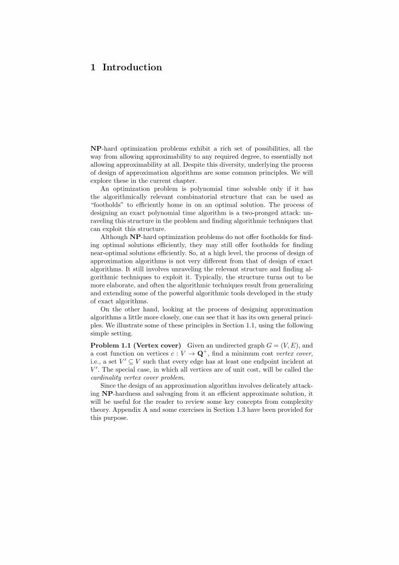
What if G is not restricted to be bipartite? In this case, a maximummatching may be strictly smaller than a minimum vertex cover. For instance,if G is simply an odd length cycle on 2p + 1 vertices, then the size of a max-imum matching is p, whereas the size of a minimum vertex cover is p + 1.This may happen even for graphs having a perfect matching, for instance,the Petersen graph:

�

�

�� �

�

�

�

�

�

��

���

������

����

��

���

��

����

��

���

��

����

��

���

�� ��

This graph has a perfect matching of cardinality 5; however, the minimumvertex cover has cardinality 6. One can show that there is no vertex cover ofsize 5 by observing that any vertex cover must pick at least p + 1 verticesfrom an odd cycle of length 2p + 1, just to cover all the edges of the cycle,and the Petersen graph has two disjoint cycles of length 5.

Under the widely believed assumption that NP �= co-NP, NP-hard prob-lems do not have No certificates. Thus, the minimum vertex cover problem ingeneral graphs, which is NP-hard, does not have a No certificate, assumingNP �= co-NP. The maximum matching problem in general graphs is in P.However, the No certificate for this problem is not a vertex cover, but a moregeneral structure: an odd set cover.

An odd set cover C in a graph G = (V, E) is a collection of disjoint oddcardinality subsets of V , S1, . . . , Sk, and a collection v1, . . . , vl of vertices suchthat each edge of G is either incident at one of the vertices vi or has bothendpoints in one of the sets Si. The weight of this cover C is defined to bew(C) = l +

∑ki=1 (|Si| − 1)/2. The following min–max relation holds.

1.3 Exercises 7

Theorem 1.7 In any graph, maxmatching M

|M | = minodd set cover C

w(C).

As shown above, in general graphs a maximum matching can be smallerthan a minimum vertex cover. Can it be arbitrarily smaller? The answer is“no”. A corollary of Theorem 1.3 is that in any graph, the size of a maximummatching is at least half the size of a minimum vertex cover. More precisely,Theorem 1.3 gives, as a corollary, the following approximate min–max rela-tion. Approximation algorithms frequently yield such approximate min–maxrelations, which are of independent interest.

Corollary 1.8 In any graph,

maxmatching M

|M | ≤ minvertex cover U

|U | ≤ 2 ·(

maxmatching M

|M |)

.

Although the vertex cover problem does not have No certificate under theassumption NP �= co-NP, surely there ought to be a way of certifying that(G, k) is a “no” instance for small enough values of k. Algorithm 1.2 (moreprecisely, the lower bounding scheme behind this approximation algorithm)provides such a method. Let A(G) denote the size of vertex cover output byAlgorithm 1.2. Then, OPT(G) ≤ A(G) ≤ 2 · OPT(G). If k < A(G)/2 thenk < OPT(G), and therefore (G, k) must be a “no” instance. Furthermore,if k < OPT(G)/2 then k < A(G)/2. Hence, Algorithm 1.2 provides a Nocertificate for all instances (G, k) such that k < OPT(G)/2.

A No certificate for instances (I, B) of a minimization problem Π satis-fying B < OPT(I)/α is called a factor α approximate No certificate. As inthe case of normal Yes and No certificates, we do not require that this certifi-cate be polynomial time computable. An α factor approximation algorithmA for Π provides such a certificate. Since A has polynomial running time,this certificate is polynomial time computable. In Chapter 27 we will showan intriguing result – that the shortest vector problem has a factor n approx-imate No certificate; however, a polynomial time algorithm for constructingsuch a certificate is not known.

1.3 Exercises

1.1 Give a factor 1/2 algorithm for the following.

Problem 1.9 (Acyclic subgraph) Given a directed graph G = (V, E), picka maximum cardinality set of edges from E so that the resulting subgraph isacyclic.Hint: Arbitrarily number the vertices and pick the bigger of the two sets,the forward-going edges and the backward-going edges. What scheme are youusing for upper bounding OPT?

8 1 Introduction

1.2 Design a factor 2 approximation algorithm for the problem of finding aminimum cardinality maximal matching in an undirected graph.Hint: Use the fact that any maximal matching is at least half the maximummatching.

1.3 (R. Bar-Yehuda) Consider the following factor 2 approximation algo-rithm for the cardinality vertex cover problem. Find a depth first search treein the given graph, G, and output the set, say S, of all the nonleaf verticesof this tree. Show that S is indeed a vertex cover for G and |S| ≤ 2 · OPT.Hint: Show that G has a matching of size |S|.

1.4 Perhaps the first strategy one tries when designing an algorithm for anoptimization problem is the greedy strategy. For the vertex cover problem,this would involve iteratively picking a maximum degree vertex and removingit, together with edges incident at it, until there are no edges left. Show thatthis algorithm achieves an approximation guarantee of O(log n). Give a tightexample for this algorithm.Hint: The analysis is similar to that in Theorem 2.4.

1.5 A maximal matching can be found via a greedy algorithm: pick an edge,remove its two endpoints, and iterate until there are no edges left. Does thismake Algorithm 1.2 a greedy algorithm?

1.6 Give a lower bounding scheme for the arbitrary cost version of the vertexcover problem.Hint: Not easy if you don’t use LP-duality.

1.7 Let A = {a1, . . . , an} be a finite set, and let “≤” be a relation onA that is reflexive, antisymmetric, and transitive. Such a relation is calleda partial ordering of A. Two elements ai, aj ∈ A are said to be comparableif ai ≤ aj or aj ≤ ai. Two elements that are not comparable are said tobe incomparable. A subset S ⊆ A is a chain if its elements are pairwisecomparable. If the elements of S are pairwise incomparable, then it is anantichain. A chain (antichain) cover is a collection of chains (antichains)that are pairwise disjoint and cover A. The size of such a cover is the numberof chains (antichains) in it. Prove the following min–max result. The size ofa longest chain equals the size of a smallest antichain cover.Hint: Let the size of the longest chain be m. For a ∈ A, let φ(a) denote thesize of the longest chain in which a is the smallest element. Now, considerthe partition of A, Ai = {a ∈ A | φ(a) = i}, for 1 ≤ i ≤ m.

1.8 (Dilworth’s theorem, see [195]) Prove that in any finite partial order,the size of a largest antichain equals the size of a smallest chain cover.Hint: Derive from the Konig-Egervary Theorem. Given a partial order on n-element set A, consider the bipartite graph G = (U, V, E) with |U | = |V | = nand (ui, vj) ∈ E iff ai ≤ aj .

1.3 Exercises 9

The next ten exercises are based on Appendix A.

1.9 Is the following an NP-optimization problem? Given an undirectedgraph G = (V, E), a cost function on vertices c : V → Q+, and a positiveinteger k, find a minimum cost vertex cover for G containing at most kvertices.Hint: Can valid instances be recognized in polynomial time (such an instancemust have at least one feasible solution)?

1.10 Let A be an algorithm for a minimization NP-optimization problem Πsuch that the expected cost of the solution produced by A is ≤ αOPT, for aconstant α > 1. What is the best approximation guarantee you can establishfor Π using algorithm A?Hint: A guarantee of 2α − 1 follows easily. For guarantees arbitrarily closeto α, run the algorithm polynomially many times and pick the best solution.Apply Chernoff’s bound.

1.11 Show that if SAT has been proven NP-hard, and SAT has been reduced,via a polynomial time reduction, to the decision version of vertex cover, thenthe latter is also NP-hard.Hint: Show that the composition of two polynomial time reductions is alsoa polynomial time reduction.

1.12 Show that if the vertex cover problem is in co-NP, then NP = co-NP.

1.13 (Pratt [222]) Let L be the language consisting of all prime numbers.Show that L ∈ NP.Hint: Consider the multiplicative group modn, Z∗

n = {a ∈ Z+ | 1 ≤ a <n and (a, n) = 1}. Clearly, |Z∗

n| ≤ n − 1. Use the fact that |Z∗n| = n − 1 iff

n is prime, and that Z∗n is cyclic if n is prime. The Yes certificate consists

of a primitive root of Z∗n, the prime factorization of n − 1, and, recursively,

similar information about each prime factor of n − 1.

1.14 Give proofs of self-reducibility for the optimization problems discussedlater in this book, in particular, maximum matching, MAX-SAT (Problem16.1), clique (Problem 29.15), shortest superstring (Problem 2.9), and Mini-mum makespan scheduling (Problem 10.1).Hint: For clique, consider two possibilities, that v is or isn’t in the optimalclique. Correspondingly, either restrict G to v and its neighbors, or removev from G. For shortest superstring, remove two strings and replace themby a legal overlap (may even be a simple concatenation). If the length ofthe optimal superstring remains unchanged, work with this smaller instance.Generalize the scheduling problem a bit – assume that you are also giventhe number of time units already scheduled on each machine as part of theinstance.

10 1 Introduction

1.15 Give a suitable definition of self-reducibility for problems in NP, i.e.,decision problems and not optimization problems, which enables you to ob-tain a polynomial time algorithm for finding a feasible solution given anoracle for the decision version, and moreover, yields a self-reducibility treefor instances.Hint: Impose an arbitrary order among the atoms of a solution, e.g., forSAT, this was achieved by arbitrarily ordering the n variables.

1.16 Let Π1 and Π2 be two minimization problems such that there is anapproximation factor preserving reduction from Π1 to Π2. Show that if thereis an α factor approximation algorithm for Π2 then there is also an α factorapproximation algorithm for Π1.Hint: First prove that if the reduction transforms instance I1 of Π1 toinstance I2 of Π2 then OPTΠ1(I1) = OPTΠ2(I2).

1.17 Show that

L ∈ ZPP iff L ∈ (RP ∩ co-RP).

1.18 Show that if NP ⊆ co-RP then NP ⊆ ZPP.Hint: If SAT instance φ is satisfiable, a satisfying truth assignment for φcan be found, with high probability, using self-reducibility and the co-RPmachine for SAT. If φ is not satisfiable, a “no” answer from the co-RPmachine for SAT confirms this; the machine will output such an answer withhigh probability.

1.4 Notes

The notion of well-characterized problems was given by Edmonds [69] andwas precisely formulated by Cook [51]. In the same paper, Cook initiated thetheory of NP-completeness. Independently, this discovery was also made byLevin [186]. It gained its true importance with the work of Karp [164], show-ing NP-completeness of a diverse collection of fundamental computationalproblems.

Interestingly enough, approximation algorithms were designed even beforethe discovery of the theory of NP-completeness, by Vizing [255] for the min-imum edge coloring problem, by Graham [113] for the minimum makespanproblem (Problem 10.1), and by Erdos [73] for the MAX-CUT problem (Prob-lem 2.14). However, the real significance of designing such algorithms emergedonly after belief in the P �= NP conjecture grew. The notion of an approx-imation algorithm was formally introduced by Garey, Graham, and Ullman[91] and Johnson [150]. The first use of linear programming in approximation

1.4 Notes 11

algorithms was due to Lovasz [192], for analyzing the greedy set cover algo-rithm (see Chapter 13). An early work exploring the use of randomization inthe design of algorithms was due to Rabin [224] – this notion is useful in thedesign of approximation algorithms as well. Theorem 1.7 is due to Edmonds[69] and Algorithm 1.2 is due to Gavril [93].

For basic books on algorithms, see Cormen, Leiserson, Rivest, and Stein[54], Papadimitriou and Steiglitz [217], and Tarjan [246]. For a good treatmentof min–max relations, see Lovasz and Plummer [195]. For books on approx-imation algorithms, see Hochbaum [126] and Ausiello, Crescenzi, Gambosi,Kann, Marchetti, and Protasi [17]. Books on linear programming, complexitytheory, and randomized algorithms are listed in Sections 12.5, A.6, and B.4,respectively.