viii. capital budgeting: advanced topics a. adjusted
TRANSCRIPT
1
VIII. Capital Budgeting: Advanced Topics
A. Adjusted Present Value Many projects under consideration by a firm may have impacts not immediately apparent under a simple NPV analysis. It may be useful to extend the simple NPV case (base case NPV) to account for these effects by computing an adjusted present value (APV) as follows:
APV = base case NPV + NPV of side effects Among the potential capital budgeting side effects are changes in the firm's borrowing capacity, costs of obtaining financing and tax shields associated with financing. Typically, the APV model is used when the investment and financing decisions cannot be separated. For example, if a firm should need to borrow in order to finance a project, interest payments on the loan may be tax deductible. The present value of the tax savings represents the adjustment for net present value purposes. For example, suppose a firm borrows to finance its investment into a project. The APV is determined as follows:
APV = base case NPV + PV tax shield = base case NPV + τ × INV where τ represents the corporate tax rate and INV represents the amount of the project investment. Sometimes discount rates can be adjusted to account for these side effects as an alternative to computing APV's. B. Projects with Different Life Expectancies In earlier sections, we considered mutually exclusive projects with identical life expectancies. If projects have identical life expectancies, or if they are not to be replicated, the standard NPV approach discussed earlier is appropriate for decision-making. However, if project lives are different, and projects (equipment etc.) are to be replaced at the end of their expected lives, some accounting for replacements must be made in the capital budgeting analysis. For example, consider a case where Project A with a 3 year life expectancy and a base case NPV of $100 is being compared to Project B with a 4 year life expectancy and a base case NPV of 125. (Here, base case NPV refers to the NPV of the project without replication or replacement.) Suppose these projects will be replicated at the end of their life expectancies and have discount rates equal to 10%. This process is assumed to continue forever. Based on a simple NPV analysis, Project B is preferred to Project A, despite the fact that we are able to replicate Project A after 3 years while we must wait 4 years to replicate Project B. There are three simple means for accounting for differences in project life expectancies: 1. Determine a common multiple for project life expectancies. For example, both Projects A
and B above would be replaced after the twelfth year. Project NPV could be computed and compared for both projects over twelve year periods.
2. Assume that both projects will be replicated at the end of each of their life expectancies forever (perpetual project replication). Since infinity is a common multiple for all life expectancies, this alternative is simply a variation on the first one above.

2
3. Compute equivalent annual annuities for each of the two projects. This means that each of the project NPVs will be computed and then, based on an amortization formula, equated to constant annuities. The project with the higher constant annuity is preferred.
Finite Period Replication If the first alternative were pursued, the two projects could be evaluated over a span of twelve years. Project A would be replicated four times and Project B would be replicated three times over this twelve-year period:
99.273)10.1(
100
)10.1(
100
)10.1(
100100
963=
++
++
++=ANPV
69.268)10.1(
125
)10.1(
125125
84=
++
++=BNPV
Since Project A has the higher NPV, it is preferred. Note that NPVs are calculated for twelve-year periods for both Projects A and B. Perpetual Replication Alternatively, we could pursue the second procedure above by assuming perpetual project replication. Assuming that these projects are replicated at the end of their expected lives forever, the NPV's of Projects A and B are found as follows:
K++
++
++
++
+=12963 )10.1(
100
)10.1(
100
)10.1(
100
)10.1(
100100ANPV
K++
++
++
+=1284 )10.1(
125
)10.1(
125
)10.1(
125125BNPV
The above equations represent infinite series that can be simplified with the use of a geometric expansion. Define Dn as a discount function; that is, Dn = 1/(1+k)n. D3 for Project A equals .7513 and D4 for project B equals .6830. The discount function will reflect the timing of replication for each project. Thus, for project A, we may write the discount function for k=.10 and t=12 years as follows: D12 = D = [1/(1+.10)3]4 = 1/(1+.10)12. We can think the first investment into one of the projects described above as being an investment into an n year project with an NPV equal to NPV(n,1). If the project is to be replicated an infinite number of times, its NPV might be written as NPV(n,∞). Each time the project is replicated, the discount function Dt is revised. Thus, in this case, a series similar to one presented above might be written as follows:
NPV(n,∞) = NPV(n,1)[1 + Dn + Dn2 + Dn
3 + ...] For Project A, the following series applies:
NPVA = 100 [1 + .7513 + .75132 + .75133 + .75134 + ...] For Project B, the following series applies:
NPVB = 125 [1 + .6830 + .68302 + .68303 + ...]

3
To simplify these series and find solutions, we perform a geometric expansion on the following: (A) NPV(n,∞) = NPV(n,1)[1 + Dn + Dn
2 + Dn3 + ...]
First, we multiply both sides of this equation by Dn: (B) NPV(n,∞) Dn = NPV(n,1)[Dn + Dn
2 + Dn3 + Dn
4 + ...] Next, we subtract Equation A from Equation B to obtain: (C) NPV(n,∞) (Dn –1) = NPV(n,1)[-1] We rewrite Equation C to obtain:
(D) 11
)1,(
1
1)1,(),(
D
nNPV
D
nNPVnNPV
n −=
−
−×=∞
Equation D is the perpetual replication formula. Filling in figures given earlier, we find NPV's for Projects A and B as follows:
(E) 09.4027513.1
100),3( =
−=∞ ANPV
(F) 32.3946830.1
125),4( =
−=∞ BNPV
We find that Project A is preferred to Project B even though its base case NPV is lower. However, our replication process ensures that our analysis accounts for project replacements in the future; NPV accounting for these replacements is higher for Project A. Thus, the procedure for using NPV for comparing mutually exclusive projects with different life expectancies is as follows: 1. First, compute the base case NPV for each project. For the base case NPV
computation, we do not assume that the project will be replicated. If this is true, we do not need to proceed to the next step. If projects are to be replicated, we proceed to the second step.
2. If projects are to be perpetually replicated on a constant scale basis (that is, NPV's for future project re-investments are the same as for the original project), we use the constant scale replication factor NPV(n,∞) to determine the value of the perpetuities associated with the projects.
4. If project NPV's are projected to grow over time, we must derive a growth replication factor.
In many instances, one can obtain results based on either IRR or annual equivalent costs for a single investment that are consistent with the results based on the constant scale replication model described above. The annual equivalent cost is the annual cash flow that sets NPV's of projects equal to zero based on a required rate of return.

4
Equivalent Annual Annuities Finally, we can evaluate the two projects using equivalent annual annuity procedures. We have determined base case NPVs for both projects. Now, we merely use present value annuity formulas to solve for the annual payments that have the same present values as the projects (PMT):
+−
=
nkkk
NPVPMT
)1(
11
21.40
)1.1(1.
1
1.
1
100
3
=
+−
=APMT
43.39
)1.1(1.
1
1.
1
125
4
=
+−
=BPMT
Project A, if replicated forever, would have the same value as a $40.21 perpetuity. Project B, if replicated forever, would have the same value as a $39.43 perpetuity. Since Project A has the higher equivalent annuity payment, it is preferred to project B. C. The Duration Problem One interesting type of capital budgeting problem is concerned with the optimal timing associated with performing a specific task (This is sometimes referred to as the capital deepening problem or duration problem). Often, this type of problem is concerned with the optimal time to initiate or terminate a project. In a sense, such a project can be analogous to comparing projects with different life expectancies. In a sense each potential life expectancy is much like a separate project. In theory, one could find the NPV associated with initiating or terminating the project at each potential life expectancy. That life expectancy with the highest NPV is optimal. Obviously, this procedure can be computationally cumbersome. Finding an appropriate continuous discounted cash flow function, typically by using calculus, significantly improves computational efficiency. Analysts are frequently interested in problems like determining the optimal time to harvest timber, replace a machine, to enter a market, sell an asset or to age wine or some other commodity. Frequently, the cash flow associated with an asset is expected to be a function of time. For example, suppose that the sales price or revenue associated with a bottle of wine increases with its age (t) as follows:
tv =Re Note that as the wine ages, its sales price increases. Further suppose that a continuous time discount function is used to discount revenues as follows:
ktCFePV −= ktktkt
t etetevPV−−− =×=×= 5.Re
Continuous discount functions are often used for such problems because they frequently discount

5
more accurately and that they are more adaptable to maximization through differentiation. Thus, in this example, we see that revenues increase with the age of the wine, though the winemaker must wait for his revenues as the wine ages. Again, it will be preferable to use the continuous time discount function for duration problems because it enables us to more easily use Calculus to derive optimal duration decisions. To find the optimal aging period, one finds a derivative of PV with respect to t and sets this derivative equal to zero:
0
5.
5. 5.5. =
−
=−=∂
∂ −−−
kt
ktkt
e
tkt
ektett
PV tkt
=5.
Multiplying both sides of the second equation above by the square root of t and simplifying, we obtain:
.5 = kt ; t = .5/k Thus, if the discount rate for the wine were 10%, the optimal aging period would be (.5/.10) = 5 years.
D. Multi-Stage Growth Models
In many types of capital budgeting problems, particularly those involving long periods of time, different growth rates might apply to the cash flows during the various stages of the project. The growth models that we discussed in the previous chapter work well for single stage growth problems, but here we discuss multiple stage models. The analyst attempts to determine the value of the project by forecasting and discounting the project’s cash flows. The following is the most general of the simple cash flow discount models:
(1) ∑∞
= +=
1 )1(tt
t
k
CFPV
This expression allows the user to input an appropriate cash flow CFt for each period t and discount that flow. The discounted cash flows for each year are then added to find the project present value PV. Obviously, adding an infinite series of cash flows is potentially cumbersome.
If the series of cash flows can be simplified by applying a constant compound growth rate to them, it may be computationally efficient to use some form of a perpetuity model to value the project. The following is an example of a one-stage perpetual growth model:
(2) gk
CFPV
−= 1
This expression can be applied only the cash flow in the first year CF1 is know, and a constant compound growth rate can be applied to following cash flows extending forever.
Suppose a company has the opportunity to invest in a business operation selling for $100 million. The operation is expected to throw off a $1.8 million cash flow next year (at the end of year 1). In each subsequent year forever, the annual cash flow is expected to grow at a rate of 4%. All cash flows are to be discounted at an annual rate of 6%. Should the operation be purchased at its current price? The following is computed from Equation 2:

6
millionmillion
PV 90$)04.06(.
8.1$=
−=
Since the $100 million purchase price of the operation is more than its $90 million value,
the operation should not be purchased. This one-stage growth model, also known as the Gordon Growth Model requires three inputs, CF1, k and g. The model is quite sensitive to each of these three inputs and to errors in estimating them. The growth rate, which should be stable to use the model, is frequently the most difficult input to estimate. However, if the growth rate can be estimated and is expected to be stable, the model may work reasonably well. For example, if economic growth was estimated to be 4%, and the company was expected to grow at the economy’s rate (e.g., in some cases, a mature company that processes food), the model may work well.
Consider a second scenario where the cash flows of an operation cannot be expected to
grow at the same rate forever. In this second scenario, suppose the operation’s cash flows grow at an annual rate of g1 for n years and then at a rate of g2 forever afterwards. The single stage growth model represented by equation (2) must be revised to account for two stages of growth. The first stage will be represented by an n year growing annuity at rate g1 and the second stage will be a growing perpetuity at a different growth rate g2. This second stage of cash flows is a deferred perpetuity that will be discounted a second time (by dividing by (1+k)n ) because it will not start until after the first n year period ends:
(3) n
n
n
n
kgk
ggCF
kgk
g
gkCFPV
)1)((
)1()1(
)1)((
)1(1
2
21
11
1
1
11
+−
+++
+−
+−
−=
−
Now, suppose a company has the opportunity to invest in an operation currently selling for
$100,000. The operation is expected to generate a $3,000 cash flow next year (at the end of year 1). In each subsequent year until the seventh year, the annual cash flow is expected to grow at a rate of 20%. Starting in the eighth year, the annual cash flow will grow at an annual rate of 3% forever. All cash flows are to be discounted at an annual rate of 10%. Should the operation be purchased at its current price? The following Two Stage Growth Model can be used to evaluate this operation:
n
n
n
n
kgk
ggCF
kgk
g
gkCFP
)1)((
)1()1(
)1)((
)1(1
2
21
11
1
1
110
+−
+++
+−
+−
−=
−
4519.801,92$)1.1)(03.1(.
)03.1()2.1(000,3$
)1.1)(2.1(.
)2.1(
2.1.
1000,3$
7
6
7
7
0 =+−
+++
+−
+−
−=P
Since the $100,000 purchase price of the operation exceeds its 92,801.4519 value, the operation should not be purchased. This two-stage model may work well for a company with established markets and brands, but where the industry is expected to enter a phase of lower growth associated with its maturity.

7
The three-stage growth model (used extensively by investment advisory services such as Value Line, Inc.) is developed as follows:
)2()1(3
3)2(
21)1(
11
)2()1(2
1)2(2
1)1(1
2)1(
21)1(
11)1(
1
)1(1
110
)1)((
)1()1()1(
)1)((
)1()1(
)()1(
)1()1(
)1)((
)1(1
nn
nn
nn
nn
n
n
n
n
kgk
gggCF
kgk
gg
gkk
ggCF
kgk
g
gkCFP
+
−
+
+−−
+−
++++
+−
++−
−+
+++
+−
+−
−=
This model is three parts:
1. An n(1) year growing annuity at a growth rate of g1 2. An [n(2)-n(1)] year growing annuity starting after n(1)-1 years of growth at rate g1 and one
year at rate g2. This second annuity, discounted a second time for n(1) years grows at rate g2.
3. A perpetuity growing at rate g3. This perpetuity is discounted for n(1)+n(2) years because it starts after the second growing annuity terminates.
Now, suppose that another company has the opportunity to invest in an operation currently
selling for $100,000. The operation is expected to throw off a $5,000 cash flow next year (at the end of year 1). In each subsequent year until the third year, the annual cash flow is expected to grow at a rate of 15%. Starting in the fourth year, the annual cash flow will grow at an annual rate of 6% until the sixth year. Starting in the seventh year, cash flows will not grow. All cash flows are to be discounted at an annual rate of 8%. Should the operation be purchased at its current price?
1078.017,92$)08.1)(008.0(
)01()06.1()15.1(000,5$
)08.1)(06.08(.
)06.1()15.1(
)06.08(.)08.1(
)06.1()15.1(5000$
)08.1)(15.08.0(
)15.1(
15.08.
1000,5$
6
313
6
1313
3
13
3
3
0
=+−
++++
+−
++−
−−
+++
+−
+−
−=
−
+−−
P
Since the $100,000 purchase price of the operation exceeds its $92,017.1 value, the operation should not be purchased.
Each of the cash flow growth models that we presented thus far has assumed that the
operation will throw off cash flows, operation value will be based on these cash flows and that all cash flows into perpetuity will have been considered. This assumption can be quite sensible; the price a company should be willing to pay for operation should be based on the value of what she receives (including whatever cash flows that subsequent shareholders receives if the shares are sold) from the firm.
Now, consider a slightly different type of situation. Suppose that Operation A were expected to generate a $10 cash flow in each of the next three years and then be sold for $100 at the end of three years. We can value the cash flows as a constant three-year annuity and then add the present value of the anticipated selling price to obtain a value of $82.61:

8
61.82$)18.1(
100$
)18.1(
11
18.
10$
)18.1(
100$10$
)18.1(
10$
)18.1(
10$33321
=+
+
+−⋅=
+
++
++
+=APV
Thus, the value of the operation equals the sum of present values of its anticipated cash flows and selling price. Consider a second example where a firm is expected to throw off cash flows to shareholders of $100,000 in one year. Subsequent cash flows are expected to grow at an annual rate of 20 percent until the end of the fourth year and then at 3 percent until the end of the 10th year. All cash flows are discounted at 10 percent. Table 4 illustrates the cash flows, their present values and cumulative present values
Table 4:
Two-Stage Growth Model Illustration
Cash Flow Series to Year (t):
Computations
Year CF(t) PV[CF(t)] SUM(PV's) 1 100000 90909.1 90909.09 2 120000 99173.6 190082.6 3 144000 108189 298272 4 172800 118025 416296.7 First
Stage
PV 5 177984 110514 526810.8 6 183324 103481 630292.1 7 188823 96896.2 727188.3 8 194488 90730.1 817918.3 9 200323 84956.3 902874.7
10 206332 79550 982424.7 Total
PV
Using Equation 4 above, this present value can be computed as follows:
425,982)1.1()1.1)(03.1(.
)03.1()2.1(
)03.1(.)1.1(
)03.1()2.1(000,100
)1.1)(2.1(.
)2.1(
2.1.
1000,100
64
1614
4
14
4
4
0
=
++−
++−
−+
+++
+−
+−
−=
+−−
P
The example above ignores cash flows anticipated after the second stage. This is
appropriate only if the firm is not expected to produce cash flows after the 10th year; we assume in

9
this example that the firm has no value after 10 years. If this were not true, we would estimate the firm’s value 10 years from now and discount it, adding this discounted terminal value to the present values of the cash flows obtained for the first 10 years. E. Capital Budgeting in the International Arena
The financial manager's capital budgeting decision concerns which projects (or other investments) will be undertaken by the firm, how much capital will be budgeted towards each of these projects and when these investments will be undertaken. Capital budgeting in the international arena is more complex than in the domestic environment due to the following: 1. Cash flows generated by a foreign project will probably be in a currency different from that
of the parent firm. 2. Cash flows of the foreign project may be subject to different tax codes and exchange
controls. For example, in some countries, profits are subject to repatriation; that is, the parent firm cannot remove its cash flows from the country where they are generated. Tax codes and regulations established by foreign governments affecting multi-national firms are often established to motivate them to re-invest their profits locally.
3. Determining proper discount rates and risk adjustments for foreign projects is complicated by fluctuating exchange rates, different riskless return rates, market returns and by varying country and currency risks. Determining costs of capital can be equally ambiguous.
4. Accounting for foreign product prices, revenues, costs, taxes and profits is more complicated than for the domestic project.
We should note that there are several methods available to the multi-national firm to transfer profits subject to repatriation from its subsidiary's country of operation. One method is for the foreign subsidiary to make interest payments (often at above-market rates) on debt to the parent firm. Second, there are often goods and services transferred between the parent firm and its foreign subsidiary. Profits from the sale or transfer of these goods and services can often be allocated where the parent firm wishes, in some cases, by setting prices that differ from market prices. Since both the parent and subsidiary firms have the same ownership, they should be unconcerned about the prices of goods transferred between them - except to the extent that taxes and cash flow restrictions are affected. This is the so-called transfer pricing issue. That is, the transfer pricing issue is concerned with how a multi-national firm should set prices on goods and services transferred between its units so as to minimize taxes and maximize its capital flexibility. Government policies attempting to force multi-national firms to re-invest their profits locally can create a number of problems and distortions. First, profit retention by the subsidiaries of multi-national firms can lead to growth of subsidiaries relative to local firms, in some cases inhibiting the abilities of local firms to compete. Secondly, multi-national firms will use transfer pricing and other strategies to shift and disguise their profits, causing a number of distortions, including many related to real production activities. Nonetheless, it is important to evaluate cash flows generated by a foreign project both from the perspective of the project and from the perspective of the parent firm. In addition, the financial manager should consider operations exposure, transactions exposure and translation exposure, all of which we discussed earlier.
10
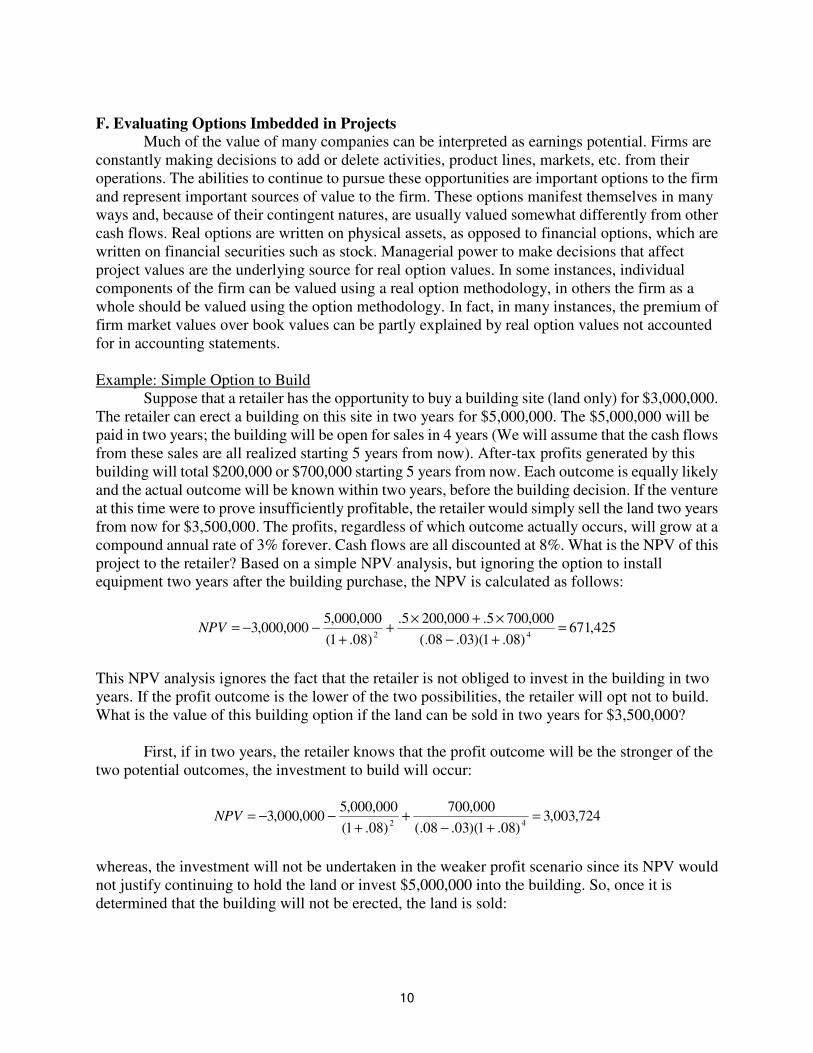
F. Evaluating Options Imbedded in Projects
Much of the value of many companies can be interpreted as earnings potential. Firms are constantly making decisions to add or delete activities, product lines, markets, etc. from their operations. The abilities to continue to pursue these opportunities are important options to the firm and represent important sources of value to the firm. These options manifest themselves in many ways and, because of their contingent natures, are usually valued somewhat differently from other cash flows. Real options are written on physical assets, as opposed to financial options, which are written on financial securities such as stock. Managerial power to make decisions that affect project values are the underlying source for real option values. In some instances, individual components of the firm can be valued using a real option methodology, in others the firm as a whole should be valued using the option methodology. In fact, in many instances, the premium of firm market values over book values can be partly explained by real option values not accounted for in accounting statements. Example: Simple Option to Build
Suppose that a retailer has the opportunity to buy a building site (land only) for $3,000,000. The retailer can erect a building on this site in two years for $5,000,000. The $5,000,000 will be paid in two years; the building will be open for sales in 4 years (We will assume that the cash flows from these sales are all realized starting 5 years from now). After-tax profits generated by this building will total $200,000 or $700,000 starting 5 years from now. Each outcome is equally likely and the actual outcome will be known within two years, before the building decision. If the venture at this time were to prove insufficiently profitable, the retailer would simply sell the land two years from now for $3,500,000. The profits, regardless of which outcome actually occurs, will grow at a compound annual rate of 3% forever. Cash flows are all discounted at 8%. What is the NPV of this project to the retailer? Based on a simple NPV analysis, but ignoring the option to install equipment two years after the building purchase, the NPV is calculated as follows:
425,671)08.1)(03.08(.
000,7005.000,2005.
)08.1(
000,000,5000,000,3
42=
+−
×+×+
+−−=NPV
This NPV analysis ignores the fact that the retailer is not obliged to invest in the building in two years. If the profit outcome is the lower of the two possibilities, the retailer will opt not to build. What is the value of this building option if the land can be sold in two years for $3,500,000? First, if in two years, the retailer knows that the profit outcome will be the stronger of the two potential outcomes, the investment to build will occur:
724,003,3)08.1)(03.08(.
000,700
)08.1(
000,000,5000,000,3
42=
+−+
+−−=NPV
whereas, the investment will not be undertaken in the weaker profit scenario since its NPV would not justify continuing to hold the land or invest $5,000,000 into the building. So, once it is determined that the building will not be erected, the land is sold:

11
686)08.1(
000,500,3000,000,3
2=
++−=NPV
Since each scenario is equally likely, the value of the project is .5×3,003,724 + .5×(686) = 1,502,205. Thus, the option to decide on the building adds substantial value to the project: 1,502,205 – 671,425 = 830,780. Thus, $830,780 is the value of the option to build. Real Options Analysis: Asset Abandonment Option Example Consider a titanium producer that has the opportunity to purchase a mine and related mining equipment for a total of $21 million. The purchase includes a titanium mine in Florida and mining-related equipment. The mining equipment, if not used, can be sold now for $12,000,000 or at any time over the next t years to another mining company for $12,000,000 e.05 × t. The mine itself will be worthless if it is abandoned, but the equipment could be sold for $12,000,000 e.05 × t. As of now, it is not known what the yield of the mine will be. A five-year study by geologists will be undertaken to determine this. Five years from now, the mine’s prospects will be fully revealed by the study. Hence, in five years, a decision will be made as to initiating mining operations. The mine will be abandoned and the equipment sold for $12,000,000e.05×5 = $15,408,305 if the yield is revealed to be less than $12,000,000 e.05×5. In this case, the yield of the mine would simply not be large enough to justify using the mine equipment and it would make more sense to abandon the mine and sell the equipment. Geologists currently believe that the present value of the mine’s expected lifetime yield is $20,000,000, but this value will not be certain until after the five-year study. The level of uncertainty concerning the mine’s yield is high. Nevertheless, geologists estimate that there is a 65.86 percent chance that this present value will range from $14.16 million to $25.84 million, implying a payout standard deviation of $5,840,000.12 Thus, the mine’s return standard deviation is .292 based on the expected value of $20 million and a normal distribution of payouts. The actual yield of the mine could be much lower or much higher, though the standard deviation of the yield does reflect this uncertainty. The mining equipment will be used until it is worthless unless the mine is abandoned and the equipment is sold. Thus, the cost of producing titanium from the mine is using the equipment until it is worthless. Thus, the company value if it does produce from the mine equals the yield from the mine; the equipment would ultimately have zero value since it would be fully used. The current riskless return rate is 5 percent, the same as the anticipated annual increase in the equipment value. Is this mining company worth $21 million if the NPV of the present value of the expected yield of the mine is only $20 million? What is the value of the mining project? There are two ways to look at this problem. First, the mining project can be modeled as having mining equipment and a call option to extract ore from the mine in five years. If the company chooses to extract the ore, it uses up its mining equipment. Then, the exercise price of this call to extract ore is the future value of the mining equipment to be used, 15,408,305 and the call’s expiration is 5 years. Option details are summarized as follows:
1 If payouts are normally distributed, there is a 65.86% probability that the yield will be within one standard deviation of the mean. The mean or expected yield is $20 million and the standard deviation is $5.84 million. The return is expressed as a proportion of $20 million. If the mine yield were $14.16 million, it would be 29.2% less than the mine’s expected yield; if the mine yield were $25.84 million, it would be 29.2% more than the expected yield.

12
T = 5 rf = .05 X =15,408,305 S0 = 20,000,000 σ = .292 σ2 = .0853 Our first steps to value the call option are to find d1 from Equation (2) and d2 from Equation (3):
108823.15292.
5)0853.5.05(.)305,408,15/000,000,20ln(1 =
×
××++=d
455891.5292.108823.12 =×−=d Next, by either using a z-table or by using an appropriate polynomial estimating function from a statistics manual, we find normal density functions for d1 and d2: N(d1) = .866247 N(d2) = .675766 We use N(d1) and N(d1) in Equation 1 to value the call option to produce the mine as follows:
743,215,9675766.7182818.2
305,408,15866247.000,000,20
505.0 =×−×=×
c
The value of the call option to produce titanium is $9,215,743. Add this value to the $12,000,000 current value of the mining equipment to determine the value of the mining project to be $21,215,743. There is a second way to consider the option value of the mine. At present, the expected yield of the mine is $20 million, and the firm has the option to abandon the mine if its yield is ultimately proven to be less than the value of the equipment to extract the ore. If the mine is ultimately abandoned, the firm will sell the mining equipment for its future value of $15,408,305. Abandoning the mine to realize sales proceeds from the sale of mining equipment is analogous to exercising a put option on the mine for the value of the mining equipment. Thus, the value of the target firm equals $20 million plus the value of a put option to abandon it for $15,408,305. We will value this put using the put-call parity relation:
000 SXecpTr f −+=
−
743,215,1000,000,207182818.2305,408,15743,215,9 505.
0 =−×+= ×−p
Thus, the value of the put option to abandon the mine equals $1,215,743. The mine has an expected value of $20,000,000, so that the total value of the target firm is $21,215,743. This is the same value as we obtained when we valued the target as the sum of equipment value plus the call to extract ore from the mine. The value of the target firm equals $21,215,743, making it a worthy purchase at a price of $20 million.

13
Real Options Analysis: Corporate Securities as Options Here, we discuss how one might value the equity and debt securities of a leveraged firm as
combinations of options and riskless debt and how takeovers and coinsurance might affect these option values. Corporate law provides for limited liability for corporate shareholders. This limits the obligation of shareholders to creditors to the amount that shareholders have invested in the equity of the firm. Limited shareholder liability provides a valuable option to shareholders and is costly to creditors. This limited liability feature of the typical corporation increases shareholder wealth when managers increase risk-taking by managers. This increased risk-taking increases shareholder wealth by enabling shareholders to benefit from highly successful ventures. While creditors do not share proportionately in the gains of the successful venture, they do stand to lose if the risky ventures are unsuccessful. Hence, shareholders are the primary beneficiaries of a successful venture; creditors lose disproportionately in unsuccessful ventures. This increases shareholder wealth at the expense of creditors.
Key to this analysis is the notion that shareholders can be thought to have a long position on a call option on the firm's assets. If the firm does well, shareholders exercise their right to purchase the firm's assets by paying off creditors. The face value of debt (along with accrued interest) can be regarded as the exercise price of the shareholder call option on the firm's assets. The shareholder call option to purchase the firm's assets is exercised when it is realized that the firm has performed well enough such that the value of those assets exceeds the face value of debt along with accrued interest representing the exercise price of the call option. If the firm performs poorly enough such that the value of assets is exceeded by the value of the creditor obligation, shareholders default and leave the assets to creditors. In effect, they decline their right to purchase the firm's assets. Hence, shareholders can be thought to have a call option on the firm's assets that is exercised only if the firm performs well and shareholders opt to assume control of the firm's assets by settling obligations to creditors.
Now, let us consider the creditor's position. Creditors expect to receive a fixed payment. This is analogous to riskless debt. However, creditors understand that if the firm performs poorly, they must accept control of the firm's assets in exchange for indemnifying shareholder obligations. Hence, they agree to accept the firm's assets if shareholders wish to put the firm's assets to them. The creditor position is analogous to a short position in a put. Creditors must take control of the firm's assets if shareholders do not want them; otherwise, shareholders have no obligation. The exercise price associated with this put is the value (face value plus accrued interest) of the shareholder obligation to them.
The option positions described above suggest that a leveraged firm’s assets can be modeled using the put-call parity formula (See the Chapter 4 appendix) as follows:
(4) 000 pXecSTrf −+=
−
where: S0 = the total value of the firm’s assets c0 = the value of the firm’s equity, a long position on a call on the firm’s assets Xe-rfT -p0 = the value of the firm’s debt, reflecting two positions:

14
Xe-rfT = the present value of riskless debt maturing at time T p0 = the risk reduction in the firm debt value; a short position in a put on assets Thus, we model the firm as though bondholders own the firm’s assets. Shares of stock becomes call options for shareholders to purchase the firm’s assets from bondholders by paying the face value X of debt, which is, in effect, the exercise price of the call option on assets. Bondholders maintain short positions on puts to retain control of the firm’s assets by forgiving shareholder obligations to them. Real Options, Takeovers and the Coinsurance Effect
The co-insurance effect concerns the ability of creditors of each of two combining firms to obtain repayment protection from the shareholders of both firms. In effect, when two firms combine, shareholders of both firms combine their resources to repay creditors of both firms. Thus, in a merger or other combination, shareholders of each firm are not only responsible for debt repayment of their own firm, they are also jointly responsible for the debt of the counterpart firm. Creditors receive additional protection in business combinations while shareholders assume additional responsibilities to repay debt. This coinsurance represents a transfer of wealth from shareholders to creditors. If the combination of businesses increases the diversification of the combining firms as should be expected, overall asset risk is reduced. Hence, takeover combinations can be “two edge swords” for shareholders of leveraged firms. This reduced asset risk decreases shareholder wealth, who maintain call options on the firm’s assets. This wealth is transferred to creditors whose short positions in puts also benefit from reduced asset risk. Limited Liability Equity: An Example Consider a grocery distributor with $25,000,000 in assets that has the opportunity to take over a supermarket chain with $20,000,000 in assets. The distributor has $20,000,000 in zero coupon debt maturing in two years and the supermarket has $15,000,000 in zero coupon debt maturing in two years. Assume that all Black-Scholes assumptions apply to each of the two firms and their securities. The standard deviations of asset returns for the distributor and supermarket are, respectively, .4 and .5. The riskless return rate is currently .04. What will be the debt and equity values for each of the two firms? In this example, we will treat equity securities as though they are call options on firm assets, enabling shareholders to take control of the firm by paying creditors the face value of debt. If asset value is less than the face value of debt, shareholders abandon their option to take over the firm’s assets. This limited shareholder liability requires debt to be risky. In effect, creditors must forgive debt payments if shareholders wish to abandon the firm (this is bankruptcy), leaving creditors holding the firm’s assets. Hence, creditors, with their risky debt, hold a combination of riskless debt and a short position on a put on the assets of the firm. Thus, in effect, creditors have agreed to purchase the firm’s assets by forgiving debt should shareholders wish to file for bankruptcy. We will re-define the terms that we use in the Black-Scholes Model for this example. From the problem statement, we have the following for the distributor: T = 2 rf = .04

15
X =20,000,000 S0 = 25,000,000 σ= .4 σ2 = .16 Inputs for the supermarket chain are: T = 2 rf = .04 X =15,000,000 S0 = 20,000,000 σ = .5 σ2 = .25 We will start by estimating values for c0 for each firm as follows. Our first steps are to find d1 from Equation (4) and d2 from Equation (5) for the distributor: d1 = {ln(25/20) + (.04 + .5 × .16) × 2} ÷ {.4 × 2.5} = .81873 d2 = d1 - .4 × 2.5 = .253044 Next, we find normal density functions for d1 and d2: N(d1) = .7935 N(d2) = .5998 Finally, we use N(d1) and N(d1) in Equation (3) to value the equity: c0 = 25,000,000(.7935) - [20,000,000 × .923] × .5998 = 8,763,008 = equity value Next, we use put-call parity to value the short put position maintained by creditors: p0 = 8,763,008 + (20,000,000 × .923) - 25,000,000 = $2,225,335 Hence, with the risk adjustment, the value of the distributor’s risky debt is 20,000,000e-.04×2 - $2,225,335 = 18,462,328 - $2,225,335 = $16,236,992. Note that debt and equity values sum to asset value. We will repeat the calculations for the supermarket chain: d1 = {ln(20/15) + (.04 + .5 × .25) × 2} ÷ {.5 × 2.5} = .8735 N(d1) = .8088 d2 = .8735 - .5 × 2.5 = .1664 N(d2) = .5661 c0 = 20,000,000(.8088) - [15,000,000 × .923] × .5661 = 8,337,781 = equity value Next, we use put-call parity to value the short put position maintained by creditors: p0 = 8,337,781 + (15,000,000 × .923) - 20,000,000 = $2,184,526 Hence, with the risk adjustment, the value of the chain’s limited liability debt is $15,000,000e-.04×2 - 2,184,526 = 13,846,746 -$2,184,526 = $11,662,219.

16
Limited Liability Equity, Takeovers and Coinsurance: An Example Now, suppose that the two firms described above are to combine. The correlation coefficient between asset returns for the two firms is .3. What will be post-merger debt and equity values of the combined firm? Do shareholders and bondholders benefit from the combination? To answer these, we will repeat the calculations above for the combined firm. However, we will first need to determine the standard deviation of the combined firm’s assets. Since the firm’s returns are not perfectly correlated, the merger will reduce the risk levels of the firms. First, note that the combined firm’s assets will total $45,000,000, fraction 5/9 from the distributor (d) and 4/9 from the supermarket chain (s). Also note that the correlation coefficient between returns on their assets is .3. Using a simple two-security risk equation, we find that the combined firm standard deviation of returns equals .3583:
) (w ,222
d2d sdsdsdssp www ρσσσσσ 2( + ) ( + )=
3583.)3.5.4.444.556.)25.444..16 (.556 22 =⋅⋅⋅⋅2( + ⋅ ( + )⋅=pσ
Notice that the return standard deviation for the combined firm is less than those for either of the two firms operating as separate entities. Now, with the new standard deviation, we repeat the valuation calculations. Inputs for the combined firm are: T = 2 rf = .04 X =35,000,000 S0 = 45,000,000 σ = .3583 σ2 = .1284 d1 = {ln(45/35) + (.04 + .5 × .1284) × 2} ÷ {.3583 × 2.5} = .9072 N(d1) = .8178 d2 = .9072 - .3583 × 2.5 = .4004 N(d2) = .6555 c0 = 45,000,000(.8178) - [35,000,000 × .923] × .6555 = 15,621,743 = equity value Next, we use put-call parity to value the short put position maintained by creditors: p0 = 15,621,743 - 45,000,000 + (35,000,000 × 1.083) = $2,930,815 Thus, with the risk adjustment, the value of the combined chain’s limited liability debt is $35,000,000e-.04×2 – 2,930,815 = 32,309,074 - $2,930,815 = $29,378,257. Note that the combined firm equity, $15,621,743, is $1,479,046 less than their combined separate values of $8,763,008 + $8,337,781 = $17,010,789. This $1,479,046 wealth reduction to shareholders was transferred to creditors. The total debt value prior to the takeover was $27,899,210; it is now $29,378,256 = $45,000,000 - $15,621,743. Hence, the takeover reduced combined firm risk, reducing shareholder wealth and transferring it to creditors. While business combinations of leveraged firms certainly involve wealth transfers from shareholders to creditors, it is not clear from statistical data whether market values actually change

17
as suggested in our example. One complication that frequently arises in business combinations is that the risk reduction increases firms’ debt capacities. This in turn leads many firms to borrow more when they engage in takeover activity, resulting in offsetting the wealth transfer effects.

18
PROBLEMS 1. Suppose that Harlan Sporting Goods can purchase a machine to sharpen skis for $3,000 that will generate annual profits equal to $1000. This machine will last for four years and then be disposed of. Alternatively, the store can purchase a better machine for $4000 that will generate annual profits of $1000 for six years before it is retired. The machines will be replaced after their useful lives. All cash flows are to be discounted at 10%. a. Calculate base case NPVs for both machines. b. Calculate NPVs for both machines assuming that they are to be replaced and used for a
total of 12 years. c. Calculate perpetual NPVs for the two machines assuming perpetual replication. d. Calculate Equivalent annuities for the two machines. e. Which machine is superior? 2. Suppose that as a mahogany tree ages, the revenues that it can generate follows the following quadratic function:
Revt = 1000t - 10t2 Suppose that cash flows are discounted continuously at 10%. What is the optimal time to harvest a mahogany tree? 3. Suppose an investor has the opportunity to invest in a stock currently selling for $100 per share. The stock is expected to pay a $1.80 dividend next year (at the end of year 1). In each subsequent year forever, the annual dividend is expected to grow at a rate of 4 percent. All cash flows are to be discounted at an annual rate of 6 percent. Should the stock be purchased at its current price? 4. An investor believes that the dividend associated with Company X will be $15 per share next year and will grow at a compound annual rate of 20 percent for each of the following five years. For the five years following this period, he believes that dividends will grow at an annual rate of 5 percent, and then remain constant forever. He discounts cash flows at 8 percent. What should this investor be willing to pay for the stock based on his analysis? 5. Suppose an investor has the opportunity to invest in a stock currently selling for $100 per share. The stock is expected to pay a $3 dividend next year (at the end of year 1). In each subsequent year until the seventh year, the annual dividend is expected to grow at a rate of 20 percent. Starting in the eighth year, the annual dividend will grow at an annual rate of 3 percent forever. All cash flows are to be discounted at an annual rate of 10 percent. Should the stock be purchased at its current price? 6. Suppose that a regional stock exchange is considering the erection of a facility to compile, store and transmit data to its institutional customers. The exchange has the opportunity to buy this building for $6,000,000. The exchange can install computer equipment and other technology in this building starting in two years for $10,000,000. The $10,000,000 will be paid two years after the building is purchased, but before the equipment is installed. The equipment will take a year to install. The building and its equipment, once installed and operational, will be available for

2
managing the exchange’s data needs in three years (We will assume that the cash flow benefits from this equipment and technology are all realized 4 years from now). Cost savings are anticipated to increase after-tax profits by either $400,000 or $1,400,000 three years from now. It is not yet known which profit figure will be realized. Each outcome is equally likely and the actual outcome will be known within two years, before the equipment installation decision is made. If the venture at this time were to prove insufficiently profitable, the exchange would simply sell the building two years from now for $7,000,000.The profits, regardless of which outcome actually occurs, will grow at a compound annual rate of 3% forever. Cash flows are all discounted at 8%. To summarize the acquisition timeline, the building can be purchased now, two years from now, a decision will be made as to equipment installation, after which the building is immediately sold if profit projections are insufficient, in three years, the data management center can be made operational and cash flow benefits start four years from now. What is the NPV of this project to the exchange? Complete your calculations with and without recognizing the option value associated with the equipment installation. 7. Flanagan Pharmaceuticals has just committed $20,000,000 to develop a new anti-depressant. The probability that the development efforts will be successful is 50%. The firm will decide in three years whether to pursue human testing on the drug at an annual cost of $5,000,000, per year, at the end of each of four years, with the first year beginning three years from now, the first cash flow in 4 years. It will pursue human testing only if initial development efforts are successful. At present, given a successful development effort, the human testing efforts are projected to be successful with a 75% probability. If testing efforts are successful, the anti-depressant is projected to generate $10,000,000 in annual profits beginning seven years from now for twenty years. While the investment is currently carried on Flanagan’s books at its original investment of $20,000,000, what is the value of the project? Was the initial investment into product development sound? Cash flows are all discounted at 8%. 8. Consider the Dennis Company, which has $50,000,000 in assets that intends to take over Sam’s Products, which has $30,000,000 in assets. Dennis has $40,000,000 in zero coupon debt maturing in five years and Sam’s has $20,000,000 in zero coupon debt maturing in five years. Assume that all Black-Scholes assumptions apply to each of the two firms and their securities. The standard deviations of asset returns for Dennis and Sam’s are, respectively, .6 and .8. The riskless return rate is currently .04. The correlation coefficient between asset returns for the two firms is .2. What will be the post merger debt and equity values of the two firms? By how much will the merger reduce overall equity value?

3
SOLUTIONS 1.a. Base case NPVs are easily determined with present value functions as follows: NPVBase A = -3000 + 1000/(1+.10)1 + 1000/(1+.10)2 + 1000/(1+.10)3 + 1000/(1+.10)4 = 169.87 NPVBase B = -4000 + 1000/(1+.10) + 1000/(1+.10)2 + 1000/(1+.10)3 + 1000/(1+.10)4 + 1000/(1+.10)5 + 1000/(1+.10)6 = 355.26
b. Calculate NPVs based on 12 years of replication as follows:
98.320)10.1(
87.169
)10.1(
87.16987.169
84,12 =+
++
+=ANPV
80.555)10.1(
26.35526.355
6,12 =+
+=BNPV
c. Perpetual Replication NPVs are calculated as follows:
NPV(4,∞)A = 169.87/(1 - .6830) = 535.88 NPV(6,∞)B = 355.26/(1 - .5645) = 815.70
d. We compute Equivalent Annual Annuities as follows:
59.53
)1.1(1.
1
1.
1
87.169
4
=
+−
=APMT
57.81
)1.1(1.
1
1.
1
26.355
6
=
+−
=APMT
e. Each of the above figures indicates that the second machine is preferable. 2.The appropriate present value function for revenues is:
PV = (1000t - 10t2)e-.1t Using the exponent rule, power rule and product rule, this function is differentiated with respect to t as follows:
ttettet
t
PV 1.21. )1.)(101000()201000( −− −−+−=∂
∂
This expression simplifies as follows:
te
tt
t
PV1.
21201000 +−=
∂
∂ t2 – 120t + 1000 = 0
The Quadratic formula can be used to simplify this further as follows:
99.1102
10004120120 2
=×−±
=t
4
The trees should be allowed to grow for 110.99 years. 3. The following Single Stage Growth Model can be used to evaluate this stock:
)(1
0gk
DIVP
−=
)04.06(.
80.1$0
−=P
Since the $100 purchase price of the stock is less than its $90 value, the stock should not be purchased. 4. Use the following Three-Stage Growth Model:
877.413]323.1548959.677924.5[15)08.1)(008(.
)01()05.1()20.1(15$
)08.1)(05.08(.
)05.1()20.1(
)05.08(.)08.1(
)05.1()20.1(15$
)08.1)(20.08(.
)20.1(
20.08.
115$
55
515
55
1515
5
15
5
5
0
=++=+−
++++
+−
++−
−+
+++
+−
+−
−=
+
−
+
+−−
P
5. The following Two-Stage Growth Model can be used to evaluate this stock:
n
n
n
n
kgk
ggDIV
kgk
g
gkDIVP
)1)((
)1()1(
)1)((
)1(1
2
21
11
1
1
110
+−
+++
+−
+−
−=
−
8014519.92)1.1)(03.1(.
)03.1()2.1(3$
)1.1)(2.1(.
)2.1(
2.1.
13$
7
7
7
7
0 =+−
+++
+−
+−
−=P
Since the $100 purchase price of the stock exceeds its $92.8014519 value, the stock should not be purchased.
6. Based on a simple NPV analysis, but ignoring the option to install equipment two years after the building purchase, the NPV is calculated as follows:
850,342,1)08.1)(03.08(.
000,400,15.000,4005.
)08.1(
000,000,10000,000,6
42=
+−
×+×+
+−−=NPV
This NPV analysis ignores the fact that the exchange is not obliged to invest in the equipment and technology in two years. If the profit outcome is the lower of the two possibilities, the exchange will opt not to install the equipment. What is the value of this equipment installation option if the building can be sold in two years for $7,000,000? First, if in two years, the exchange knows that the profit outcome will be the stronger of the two potential outcomes, the investment to build will occur:

5
448,007,6)08.1)(03.08(.
000,400,1
)08.1(
000,000,10000,000,6
42=
+−+
+−−=NPV
whereas, the investment will not be undertaken in the weaker profit scenario since its NPV would not justify continuing to hold the building or invest $10,000,000 into the equipment and technology. So, once it is determined that the equipment will not be installed, the building is sold:
372,1)08.1(
000,000,7000,000,6
2=
++−=NPV
Since each scenario is equally likely, the value of the project is .5×6,007,448 + .5×(1,372) = 3,004,410. Thus, the option to decide later on installing the equipment adds substantial value to the project: 3,004,410 – 1,342,850 = 1,661,560. Thus, $1,661,560 is the value of the option to install equipment and technology. 7. If the development phase is successful, the present value (three years from now) of the 4-year
annuity associated with testing is $16,560,063:
630,560,16$)08.1(
11
08.
000,000,5$43 =
+−×=NPV
If the human testing phase is successful, the present value of the 20-year profit annuity seven years from now is $98,181,470:
470,181,98$)08.1(
11
08.
000,000,10$207 =
+−×=NPV
There is a 50% probability that the testing phase annuity will be incurred and a .375 probability that the drug product will be launched:
800,909,14$)08.1(
470,181,98$375.
)08.1(
630,560,16$5.73
=×
+×
−=NPV
Because this NPV is positive, the human testing will occur if the project development phase is successful. The project’s value is $14,909,800. However, this value did not justify the initial $20,000,000 in product development. The $20,000,000 book value of this project overstates its worth. 8. Inputs are as follows: Dennis: t = 5 rf = .04 X =40,000,000 S0 = 50,000,000 σ = .6 σ2 = .36 Sam’s:

6
t = 5 rf = .04 X =20,000,000 S0 = 30,000,000 σ = .8 σ2 = .64 Computations are as follows: Dennis: d1 = .986 N(d1) = .838 d2 = -.355 N(d2) = .361 c0 = $30,072,404 = equity value p0 = $12,821,634 D = $32,749,235 - $12,821,634 = $19,927,596 Sam’s: d1 = 1.232 N(d1) = .891 d2 = -.5559 N(d2) = .289 c0 = $22,001,557 = equity value p0 = $8,376,172 D = $16,374,617 - $8,376,172 = $7,998,443. Using the simple two-security risk equation, we find that the combined firm standard deviation of returns equals .525:
) (w ,222
d2d sdsdsdssp www ρσσσσσ 2( + ) ( + )=
)2.8.6.375.625.8.375..6 (.625 2222 ××××2( + )× ( + )×=pσ
Combined firm: d1 = 1.0023 N(d1) = .8419 d2 = -.1715 N(d2) = .4319 c0 = $46,137,330 = equity value p0 = $15,261,175 D = $49,123,852 - $15,261,175 = $33,862,670 Note that the combined firm equity has been reduced by $5,936,631. This wealth reduction imposed on shareholders was transferred to creditors.

7
Appendix A: A Primer on Option Pricing First, we will introduce a few option basics. A stock option is a legal contract that grants its owner the right (though, not the obligation) to either buy or sell a given stock. There are two types of stock options: puts and calls. A call grants its owner to purchase stock (called underlying shares) for a specified exercise price (also known as a striking price) on or before the expiration date of the contract. In a sense, a call is similar to a coupon that one might find in a newspaper enabling its owner to, for example, purchase a roll of paper towels for one dollar. If the coupon represents a bargain, it will be exercised and the consumer will purchase the paper towels. If the coupon is not worth exercising, it will simply be allowed to expire. The value of the coupon when exercised would be the amount by which value of the paper towels exceeds one dollar (or zero if the paper towels are worth less than one dollar). Similarly, the value of a call option at exercise equals the difference between the underlying market price of the stock and the exercise price of the call. Suppose, for example, that a call option with an exercise price of $90 currently exists on one share of stock. The option expires in one year. This share of stock is expected to be worth either $80 or $120 in one year, but we do not know which at the present time. If the stock were to be worth $80 when the call expires, its owner should decline to exercise the call. It would simply not be practical to use the call to purchase stock for $90 (the exercise price) when it can be purchased in the market for $80. The call would expire worthless in this case. If, instead, the stock were to be worth $120 when the call expires, its owner should exercise the call. Its owner would then be able to pay $90 for a share that has a market value of $120, representing a $30 profit. In this case, the call would be worth $30 when it expires. Let T designate the options term to expiry, ST the stock value at option expiry and cT be the value of the call option at expiry. The value of this call at expiry is determined as follows: (1)
],0[ XSMAXc TT −=
When ST = 80, CT = MAX[0, 80 – 90] = 0 When ST=120, CT = MAX[0, 120 – 90] = 30
A put grants its owner the right to sell the underlying stock at a specified exercise price on or before its expiration date. A put contract is similar to an insurance contract. For example, an owner of stock may purchase a put contract ensuring that he can sell his stock for the exercise price given by the put contract. The value of the put when exercised is equal to the amount by which the put exercise price exceeds the underlying stock price (or zero if the put is never exercised). To continue the above example, suppose that a put option with an exercise price of $90 currently exists on one share of stock. The put option expires in one year. Again, this share of stock is expected to be worth either $80 or $120 in one year, but we do not know which at the present time. If the stock were to be worth $80 when the put expires, its owner should exercise the put. In this case, its owner could use the put to sell stock for $90 (the exercise price) when it can be purchased in the market for $80. The put would be worth $10 in this case. If, instead, the stock were to be worth $120 when the put expires, its owner should not exercise the put. Its owner should

8
sell for $90 for a share that has a market value of $120. In this case, the call would be worth nothing when it expires. Let pT be the value of the put option at expiry. The value of this put at expiry is determined as follows: (2) pT = MAX[0, X – ST]
When ST=80, pT = MAX[0, 90 – 80] = 10 When ST=120, pT = MAX[0, 120 – 80] = 0
The owner of the option contract may exercise his right to buy or sell; however, he is not
obligated to do so. Stock options are simply contracts between two investors issued with the aid of a clearing corporation, exchange and broker that ensure that investors honor their obligations to each other. The corporation whose stock options are traded will probably not issue and does not necessarily trade these options. Investors, typically through a clearing corporation, exchange and brokerage firm, create and trade option contracts amongst themselves.
For each owner of an option contract, there is a seller or "writer" who creates the contract,
sells it to a buyer and must satisfy an obligation to the owner of the option contract. The option writer sells (in the case of a call exercise) or buys (in the case of a put exercise) the stock when the option owner exercises. The owner of a call is likely to profit if the stock underlying the option increases in value over the exercise price of the option (he can buy the stock for less than its market value); the owner of a put is likely to profit if the underlying stock declines in value below the exercise price (he can sell stock for more than its market value). Since the option owner's right to exercise represents an obligation to the option writer, the option owner's profits are equal to the option writer's losses. Therefore, an option must be purchased from the option writer; the option writer receives a "premium" from the option purchaser for assuming the risk of loss associated with enabling the option owner to exercise. Most stock options in the United States and Europe are traded on exchanges. The largest U.S. options exchange is the Chicago Board Options Exchange. The American and Philadelphia Exchanges also maintain stock options trading facilities. Options are also traded on several different commodities, currencies and other financial instruments. Options may be classified into either the European variety or the American variety. European options may be exercised only at the time of their expiration; American options may be exercised any time before and including the date of expiration. Most option contracts traded in the United States (and Europe as well) are of the American variety. We will demonstrate in the next section that American options can never be worth less than their otherwise identical European counterparts. The simple terminal value examples we discussed above were based on a Binomial
Distribution where there are two possible outcomes for a given future point in time. If we add more time periods and more trials, we would increase the number of possible terminal outcomes. As the number of trials in a binomial distribution approach infinity, the binomial distribution approaches the Normal Distribution. Black and Scholes provide a derivation for an option-pricing model
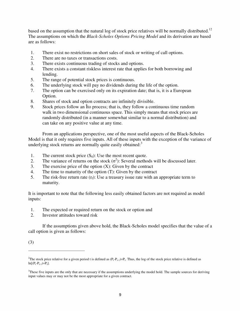
9
based on the assumption that the natural log of stock price relatives will be normally distributed.12 The assumptions on which the Black-Scholes Options Pricing Model and its derivation are based are as follows: 1. There exist no restrictions on short sales of stock or writing of call options. 2. There are no taxes or transactions costs. 3. There exists continuous trading of stocks and options. 4. There exists a constant riskless interest rate that applies for both borrowing and
lending. 5. The range of potential stock prices is continuous. 6. The underlying stock will pay no dividends during the life of the option. 7. The option can be exercised only on its expiration date; that is, it is a European
Option. 8. Shares of stock and option contracts are infinitely divisible. 9. Stock prices follow an Îto process; that is, they follow a continuous time random
walk in two dimensional continuous space. This simply means that stock prices are randomly distributed (in a manner somewhat similar to a normal distribution) and can take on any positive value at any time.
From an applications perspective, one of the most useful aspects of the Black-Scholes Model is that it only requires five inputs. All of these inputs with the exception of the variance of underlying stock returns are normally quite easily obtained:3 1. The current stock price (S0): Use the most recent quote. 2. The variance of returns on the stock (σ2): Several methods will be discussed later. 3. The exercise price of the option (X): Given by the contract 4. The time to maturity of the option (T): Given by the contract 5. The risk-free return rate (rf): Use a treasury issue rate with an appropriate term to
maturity. It is important to note that the following less easily obtained factors are not required as model inputs: 1. The expected or required return on the stock or option and 2. Investor attitudes toward risk If the assumptions given above hold, the Black-Scholes model specifies that the value of a call option is given as follows: (3)
2The stock price relative for a given period t is defined as (Pt-Pt-1)÷Pt. Thus, the log of the stock price relative is defined as ln[(Pt-Pt-1)÷Pt].
3These five inputs are the only that are necessary if the assumptions underlying the model hold. The sample sources for deriving input values may or may not be the most appropriate for a given contract.

10
)()( 2100 dNe
XdNSc
Tr f
−=
(4)
T
TrXSd
f
σ
σ )2/()/ln( 20
1
++=
(5)
Tdd σ−= 12
where N(d*) is the cumulative normal distribution function for (d*). This is function frequently referred to in a statistics setting as the "z" value for (d*). From a computational perspective, one would first work through Equation (4), then Equation (5) before valuing the call with Equation (3). N(d1) and N(d2) are areas under the standard normal distribution curves (z-values). Simply locate the z-value on an appropriate table (see Table C.1) corresponding to the N(d1) and N(d2) values. Consider the following simple example of a Black-Scholes Model application: An investor has the opportunity to purchase a six month call option for $7.00 on a stock which is currently selling for $75. The exercise price of the call is $80 and the current riskless rate of return is 10% per annum. The variance of annual returns on the underlying stock is 16%. At its current price of $7.00, does this option represent a good investment? First, we note the model inputs in symbolic form: t = .5 rf = .10 σ = .4 S0 = 75 X = 80 σ2 = .16 e 2.71828 Our first steps are to find d1 from Equation (4) and d2 from Equation (5):
1928.2828.09.5.4.12 −=−=⋅−= dd Next, by either using a z-table (see Table A.1) or by using an appropriate estimation function from a statistics manual, we find normal density functions for d1 and d2:
Next, by either using a z-table or by using the polynomial estimating function above, we find normal density functions for d1 and d2:
( ) ( )( ) ( ) 423549.1928.
535864.09.
2
1
=−=
==
NdN
NdN
Finally, we use N(d1) and N(d2) to value the call:
( )09.
2828.
09.)9375ln(.
5.4.
5.)16.5.1(.80/75ln1 =
+=
⋅
⋅⋅++=d

11
958.742.80
536.755.10.0 =×−×=
×e
C
Since the 7.958 value of the call exceeds its 7.00 market price, the call represents a good purchase. Table A.1:
The z-Table
z 0.00 0.01 0.02 0.03 0.04 0.05 0.06 0.07 0.08 0.09 0.0 .0000 .0040 .0080 .0120 .0159 .0199 .0239 .0279 .0319 .0358 0.1 .0398 .0438 .0478 .0517 .0557 .0596 .0636 .0675 .0714 .0753 0.2 .0793 .0832 .0871 .0909 .0948 .0987 .1026 .1064 .1103 .1141 0.3 .1179 .1217 .1255 .1293 .1331 .1368 .1406 .1443 .1480 .1517 0.4 .1554 .1591 .1628 .1664 .1700 .1736 .1772 .1808 .1844 .1879 0.5 .1915 .1950 .1985 .2019 .2054 .2088 .2123 .2157 .2190 .2224 0.6 .2257 .2291 .2324 .2356 .2389 .2421 .2454 .2486 .2517 .2549 0.7 .2580 .2611 .2642 .2673 .2703 .2734 .2764 .2793 .2823 .2852 0.8 .2881 .2910 .2939 .2967 .2995 .3023 .3051 .3078 .3106 .3133 0.9 .3159 .3186 .3212 .3238 .3264 .3289 .3315 .3340 .3365 .3389 1.0 .3413 .3437 .3461 .3485 .3508 .3531 .3554 .3577 .3599 .3621 1.1 .3643 .3665 .3686 .3708 .3729 .3749 .3770 .3790 .3810 .3830 1.2 .3849 .3869 .3888 .3906 .3925 .3943 .3962 .3980 .3997 .4015 1.3 .4032 .4049 .4066 .4082 .4099 .4115 .4131 .4147 .4162 .4177 1.4 .4192 .4207 .4222 .4236 .4251 .4265 .4279 .4292 .4306 .4319 1.5 .4332 .4345 .4357 .4370 .4382 .4394 .4406 .4418 .4429 .4441 1.6 .4452 .4463 .4474 .4484 .4495 .4505 .4515 .4525 .4535 .4545 1.7 .4554 .4564 .4573 .4582 .4591 .4599 .4608 .4616 .4625 .4633 1.8 .4641 .4649 .4656 .4664 .4671 .4678 .4686 .4693 .4699 .4706 1.9 .4713 .4719 .4726 .4732 .4738 .4744 .4750 .4756 .4761 .4767 2.0 .4772 .4778 .4783 .4788 .4793 .4798 .4803 .4808 .4812 .4817 2.1 .4821 .4826 .4830 .4834 .4838 .4842 .4846 .4850 .4854 .4857 2.2 .4861 .4864 .4868 .4871 .4875 .4878 .4881 .4884 .4887 .4890 2.3 .4893 .4896 .4898 .4901 .4904 .4906 .4909 .4911 .4913 .4916 2.4 .4918 .492 .4922 .4925 .4927 .4929 .4931 .4932 .4934 .4936 2.5 .4938 .4940 .4941 .4943 .4945 .4946 .4948 .4949 .4951 .4952 2.6 .4953 .4955 .4956 .4957 .4959 .4960 .4961 .4962 .4963 .4964 2.7 .4965 .4966 .4967 .4968 .4969 .4970 .4971 .4972 .4973 .4974 2.8 .4974 .4975 .4976 .4977 .4977 .4978 .4979 .4979 .4980 .4981 2.9 .4981 .4982 .4982 .4983 .4984 .4984 .4985 .4985 .4986 .4986 3.0 .4986 .4987 .4987 .4988 .4988 .4989 .4989 .4989 .4990 .4990 Put-Call Parity Before proceeding with pricing models applicable to the valuation of call options, we will first discuss a simple model concerning the relationship between put and call values. When this relationship holds, one is able to value a put based on knowledge of a call with exactly the same terms. First, assume that there exists a European put (with a current value of p0) and a European call (with a value of c0) written on the same underlying stock that currently has a value equal to X. Both options expire at time T and the riskless return rate is rf. The basic Put-Call Equivalence Formula is as follows:

12
(1)
000 pSXecTrf +=+
−
That is, a portfolio consisting of one call with an exercise price equal to X and a pure discount riskless note with a face value equal to X must have the same value as a second portfolio consisting of a put with exercise price equal to X and one share of the stock underlying both options. A very useful implication of the put call parity relation, we can easily derive the price of a put given a stock price, call price, exercise price and riskless return: (2)
000 SXecpTrf −+=
−
We can use the put-call parity relation to extend our previous example to find the value of the put as follows: t = .5 rf = .10 σ = .4 S0 = 75 X = 80 σ2 = .16 e 2.71828 p0 = c0 + Xe-rft - S0 p0 = 7.958 + 80(.9512) - 75 = 9.054
Appendix Exercises
1. Call and put options with an exercise price of $30 are traded on one share of Company X stock. a. What is the value of the call and the put if the stock is worth $33 when the options expire? b. What is the value of the call and the put if the stock is worth $22 when the options expire? c. What is the value of the call writer's obligation stock is worth $33 when the options expire?
What is the value of the put writer's obligation stock is worth $33 when the options expire? d. What is the value of the call writer's obligation stock is worth $22 when the options expire?
What is the value of the put writer's obligation stock is worth $22 when the options expire? e. Suppose that the purchaser of a call in part a paid $1.75 for his option. What was his profit
on his investment? f. Suppose that the purchaser of a call in part b paid $1.75 for his option. What was his profit
on his investment? 2. Evaluate calls and puts for each of the following European stock option series: Option 1 Option 2 Option 3 Option 4 T = 1 T = 1 T = 1 T = 2 S = 30 S = 30 S = 30 S = 30 σ = .3 σ = .3 σ = .5 σ = .3 r = .06 r = .06 r = .06 r = .06 X = 25 X = 35 X = 35 X = 35

13
Appendix Exercise Solutions
1. a. cT = $33 - $30 = $3; pT = 0 b. cT = 0; pT = $30 - $22 = $8 c. cT = -$3; pT = 0 d. cT = 0; pT = -$8 e. $3 - $1.75 = $1.25 f. $0 - $1.75 = -$1.75 2. The options are valued with the Black-Scholes Model in a step-by-step format in the following table: OPTION 1 OPTION 2 OPTION 3 OPTION 4 d(1) .957739 -.163836 .061699 .131638 d(2) .657739 -.463836 -.438301 -.292626 N[d(1)] .830903 .434930 .524599 .552365
N[d(2)] .744647 .321383 .330584 .384904
Call 7.395 2.455 4.841 4.623 Put 0.939 5.416 7.803 5.665