vighnesh anap
TRANSCRIPT

1
Artificial Neural Networks for
Classification Problem
Vighnesh Suresh Anap
Submitted for the Degree of Master of Science in
MSc in Data Science and Analytics
Department of Computer Science
Royal Holloway University of London
Egham, Surrey TW20 0EX, UK
August 30, 2015

2
Declaration
This report has been prepared on the basis of my own work. Where other
published and unpublished source materials have been used, these have been
acknowledged.
Word Count: 14,489
Student Name: Vighnesh Suresh Anap
Date of Submission: September 1, 2015
Signature:
Acknowledgements
I would like to express the deepest appreciations to my supervisor Dr. Chris Watkins
who has helped, guided and encouraged me throughout this project. His expertise
and profound knowledge of this subject, and his patience as a teacher played a huge
part in completion of this project. I am also thankful to him for giving the right
advice at the right time and for helping me shape my skills.
I am grateful to my mother who helped me to achieve my goals and for
being a source of motivation.
3
Abstract
The main aim of this experiment is to understand, investigate, and diagnose
the working of artificial neural network (ANNs) and implement neural network for
Classification problem. We studied potential benefits of using artificial neural
networks for regression using Auto dataset and classification using Thyroid disease
dataset for the diagnosis of thyroid function. Experiment also focused on analogy of
the human brain, how human neurons gave birth to artificial neurons, types of the
ANNs and types of the activation function use to train the neural nets. Further, we
studied in detail about ANN for regression and classification, the back-propagation
and feedforward algorithms with overfitting and under-fitting concept of data.
The neural networks are highly parallel systems that are capable of solving
very complicated problems that linear computing cannot handle also neural nets can
automatically extract the necessary features. One of the main reason to use artificial
neural networks in data analytics is it can scale well, many modern machine learning
techniques such as SVMs and Kernel methods have big scaling issues. To complete
our goal we will use, the Iris dataset.
To check the effectiveness of the neural net different activation function
solutions are tested. The experiment have shown that choice of the number of
hidden neurons is very crucial to achieve the success of good neural network. Each
time neural net is trained, it showed different solutions due to different initial
weights and bias parameters. The suitable activation function number of hidden
layer neurons are achieved using test and error methods. The simulation results
indicates that the performed optimization in ANNs can be reached at the 99.99% of
accuracy level. The dataset we used had previously been studied by multivariate
statistical methods and variety of pattern recognition techniques.

4
Table of Contents
1 Introduction .................................................................................................. 1
2 Background Research .................................................................................. 3
2.1 Complex Adaptive System (CAS) ............................................................ 3
2.2 Computational Intelligence (CI) ............................................................... 3
2.3 Analogy of Human Brain .......................................................................... 4
2.4 From Human Neurones to Artificial Neurones ..................................... 6
2.4.1 Step Function ............................................................................................ 7
2.4.2 Sigmoid Function ...................................................................................... 7
2.4.3 Piecewise Linear Function ........................................................................ 8
2.4.4 Gaussian Function .................................................................................... 9
2.4.5 Rectified Linear unit .................................................................................. 9
2.5 Types of Artificial Neural Networks ..................................................... 10
2.5.1 Supervised and unsupervised learning based networks ................ 10
2.5.2 Feedback and Feedforward connections based networks .............. 10
2.5.3 Feed-Forward Neural Network .......................................................... 11
2.5.4 Recurrent Neural Network ................................................................. 11
2.5.5 Radial Basis Function (RBF) Network ............................................... 12
2.5.6 Radial Basis Function (RBF) Network ............................................... 12
2.6 Neural Network Theory .......................................................................... 13
2.6.1 Network Neural Networks for Regression ....................................... 15
2.6.2 Neural Networks for Classification [37] ............................................... 25
2.6.3 Measuring of the Training Error [37] .................................................... 26
3 Experiment .................................................................................................. 27
3.1 Task ............................................................................................................ 27
3.2 Preparatory Work ..................................................................................... 27
3.2.1 Exploration ............................................................................................ 27
3.2.2 Knowledge Acquisition ....................................................................... 28
3.2.3 Datasets Used ........................................................................................ 28

5
3.3 Approach ................................................................................................... 29
3.3.1 For Satlog (Shuttle) Data Set ............................................................... 29
3.3.2 For Iris Data Set .................................................................................... 32
3.4 Results ........................................................................................................ 35
3.4.1 Results for Iris Plant Dataset ............................................................... 35
3.4.2 Results for StatLog (Shuttle) dataset .................................................. 38
3.5 Conclusion ................................................................................................. 38
3.6 Possible extension to the experiment ..................................................... 38
4 Self-Assessment ......................................................................................... 39
4.1 Strengths .................................................................................................... 39
4.2 Weaknesses ............................................................................................... 39
4.3 Opportunities ............................................................................................ 40
4.4 Threats........................................................................................................ 40
5 Professional Issue – Licensing ................................................................. 41
5.1 What is Open Source? .............................................................................. 41
5.2 What is open source software? ............................................................... 41
5.3 Licensing issues of open source software ............................................. 42
5.3.1 Copy-left vs Non-Copy-left ................................................................. 42
5.3.2 Patent Reciprocity (or: The Trade-off between Simple and
Comprehensive) ............................................................................................................... 42
5.3.3 Inbound vs Outbound ......................................................................... 43
5.4 Legal issues of open source software ..................................................... 43
6 How to use my project .............................................................................. 47
6.1 For Iris dataset .......................................................................................... 47
6.2 For Statlog (Shuttle) Code ....................................................................... 48
7 Appendix ..................................................................................................... 49
7.1 Scripts for Iris dataset code ..................................................................... 49
7.1.1 neural_net_predict R script ................................................................. 49
7.1.2 neural_net_test R script ....................................................................... 49
7.1.3 neural_net_train R script ..................................................................... 50
7.1.4 neural_net_iris_test_script R script .................................................... 54

6
7.2 Scripts for neural net using inbuilt function code ................................ 55
7.2.1 R script ................................................................................................... 55
7.2.1 R script ................................................................................................... 56

1
1 Introduction Artificial neural networks (ANNs) is an information processing paradigm that is
inspired by, how biological nervous systems process information such as brain.
These are crude electronic models based on the neural structure of the brain. The
brain basically learns various things by experience, by example. It is composed by
large number of highly interconnected processing elements (neurons) working
simultaneously to solve specific problems. ANNs also work same way as brain,
learn by experience. Donal Hebb established in 1943 that “a network of these
mathematical neurons can “learn” when exposed to the data“, and Hava Siegalmann
proved that an “ANN has the full computational capacity of a Universal Turing
Machine.” ANNs are configured for a specific problems, such as pattern
classification, data processing, regression analysis, robotics through the learning
process [7].
The development of further learning algorithms – mostly known concept of
backpropagation independently invented by Werbos and Parker in 1974 and 1982,
respectively – have made ANNs a powerful tool and highly active research area till
the date. The first neural network was developed in 1943 by the neurophysiologist
Warren McCulloch and the logician Walter Pits, but the lack of technology
availability at that time did not allow them to do progress in this field [7]. In computer
science, neural networks acquired lot of heat over the past few years in areas such
as data analytics, forecasting as well as data mining [18].
Data analytics is normally defined as the science of examining raw data with
the purpose of drawing conclusion and gaining insights about the information. The
raw data may be structured or unstructured. Data analytics is used in many different
industries to allow them make better decisions and gain insights from available data;
and in science, to verify/disprove existing theories or models [18]. Data analytics is
different from data mining in the sense of analysis by scope, focus and purpose. Data
mining is used to discover new patterns out of very big data sets which generally
stored in organization’s data warehouse and does so by applying different methods,
algorithms that devise out of statistics, database management, visualization, or
artificial intelligence. The actual data mining task considers automatic (or semi-
automatic) analysis of large quantities of data and the actual goal of the task is to
gain previously unknown or undiscovered patterns such as regression,
classification, future learning, unusual records (anomaly detection), dependencies
(association rule mining), or group of data records (cluster analysis) [18]. Hence, data
mining basically focuses on sorting through large data sets to identify the hidden
patterns and set up hidden relationships i.e. to extract value. On the other hand data
analytics focuses on inference, it is the process of deriving a conclusion which is
entirely based on consciousness of the researcher. To sum up, artificial neural
network can be describe as the highly parallel system that is capable of resolving
complicated paradigms that linear computing cannot handle [18]. Artificial neural
networks are commonly used for regression and classification in data analysis.
2
[1]The term neural network is use to encompass a large class of models and
learning methods and it is a system of programs and data structures that resembles
the operation of human brain. Most widely used neural net is “Vanilla”, sometimes
called as single hidden layer back-propagation network or a single layer perceptron.
A neural network may be of two- stage regression or classification model, which can
be represented by a network diagram [1]
In this project, we will study about the idea behind Neural Network and
how we reach from human neuron to artificial neurons. Then we will study different
types of artificial neural network. Outcomes of this project will be develop, evaluate
and use of effective machine learning methods; apply methods and techniques such
as regression, classification, and neural networks to gain exact value and insights
from data. In the implementation part of the project, we will see the implementation
of neural network for classification using backpropagation algorithm without using
any existing implementation of neural network. We will use Iris Plant dataset from
Fisher, which is perhaps the best known database to be found in Patter Recognition
literature to build the basic module for the Classification Problems, although the
program can be used for any dataset. Then we will see, neural net implementation
using the Statlog (Shuttle) dataset made available by NASA which has large volume
of the instances. Further details will be provided later part of the report. It is the
process of training a neural network to assign the correct target classes to a set of
input patterns. Once we trained the network it can be used to classify patterns that
are undiscovered before. For the code implementation we will use R. Details of the
implementation will be provided in the later part of the report [32].
I am confident about this project that it will provide me a platform for my
machine learning and data analytics journey by providing me lots of exposure to
Artificial Neural Networks. Even though neural networks have been around for
decades as I mention above they are gaining lots of steam over the past few years in
the fields such as, data analytics, prediction, as well as data mining. In my attempt
to dissect ANNs, I have got very good feeling about how they work and profound
knowledge of the same. I have also learned that how useful ANNs in the data
analytics and forecasting.
As a data analysts, we usually should have the traits such as curiosity,
imaginative, methodical, analytical, synthetical, and ability to convey our result to
our client via verbally, visually and numerically. This project has got me thinking
about these traits of our work, and allowed me to formulate some ideas and attempt
to put them into practice.

3
2 Background Research This section provides an outline of the background research conducted for the
different functions of the system. It also
2.1 Complex Adaptive System (CAS)
Complexity occurs from inter-action, inter-connectivity and inter-relationship of
elements within a system and its environment. Many natural systems for example
brain and immune system in human biology, flora and fauna in ecosystem, air and
water molecules in weather system, societies; and increasingly, many artificial
systems for example artificial intelligence system, neural networks, parallel and
distributed computing system, evolutionary programs are characterized by
apparently complex behaviour that appears as a result of often non-linear spatio-
temporal interactions among a large number of component system at different
levels of organization. These systems have recently become known as Complex
Adaptive Systems (CAS) [4].
John H. Holland said that complex adaptive system as one that displays
“coherence under change”. The details change – the antibodies in human body
change, the people in your life change – but, he contends, “Your immune system is
coherent enough to provide a satisfactory scientific definition of your identity”. The
two most important behaviours of a CAS, coherence (Robustness) and adaptation
(Learning) makes them very attractive contestant for imitation in artificial systems [4].
2.2 Computational Intelligence (CI) The field of computational intelligence which is offshoot (some says
extension, successor) of artificial intelligence in which emphasis is placed on
heuristic algorithms. The three main pillars of computational intelligence are Neural
Networks, Fuzzy Logic and Evolutionary Computation. It also encompasses
elements of adaptation, learning, heuristic and meta-heuristic optimisation, as well
as any hybrid methods which uses combination of one or more of these techniques.
It is also becoming famous in emerging areas such as swarm intelligence, chaotic
systems, artificial immune systems and others. The IEEE Computational Intelligence
Society uses the tag-line ‘Mimicking Nature for Problem Solving’ to describe
Computational Intelligence, although mimicking nature is not a necessary elements [5]. According to David Fogel, “Intelligence is the capability of a system to adapt its
behaviour* to meet its goals in a range of environments. It is a property of all
purpose-driven decision makers. Computational intelligence comprises practical
adaptation concepts, paradigms, algorithms and implementations that enable or
facilitate appropriate actions (intelligent behaviour) in complex and changing
environments” [6].

4
2.3 Analogy of Human Brain
The exact working of the human brain is still mystery and still unknown how brain
train itself to process the information. Yet, some aspect of this amazing processor are
known. In particular, the very important and most basic element of human brain is
specific type of cell which, unlike the rest of the body cells doesn’t appear to
regenerate. Because this type of cell is only body cells that isn’t slowly replaced,
assumed that these cells are what provides humans the ability to think, remember
and apply previous experiences on every actions. These cells, 100 billion of them,
are known as neurons. Each of these neurons can connect up to 100,000 other
neurons, although 1,000 to 10,000 is typical number. The brain power of the human
mind comes from the total numbers of these basic components and the multiple
connections between them. It is also comes from genetic programming, training and
learning [8].
The individual neurons has very complicated structure. They have loads of
parts, sub-systems and control mechanisms. Information conveys through host of
electrochemical pathways. It also has a thousands of different classes of neurons,
which are depends on classification methods used by them. Together these neurons
and connections among them form a process which is not binary, not synchronous
and not stable. To cut a long story short, it is nothing like the currently available
electronic computers or even artificial neural networks. These artificial neural
networks try to replicate only the most basic elements of this versatile, complicated
and powerful organism. They do it in indigenous way. But for the software engineer
who is trying to solve problems, neural computing was never about replicating
human brains. It is about machines and a new way to solve complex problems [8].
In human brain, the typical neuron collects signals from others through host
of a fine structure called dendrites. The neurons sends out spikes of electrical activity
through long and thin stand which is known as an axon, these axons are splits into
thousands of branches. At the end of each branch, a structure called a synapse
converts the activity comes from axon into electrical effects that inhibits or excite
activity from the axon into electrical effects that inhibits or excite activities into
connected neurones. When neuron receives excitatory inputs that is insufficiently
large compared with its inhibitory input, it sends a spike of electrical activity down
to its axon. Here learning is occurs by changing the effectiveness of the synapses so
that the influence of one neuron on another changes [9].

5
Figure 1: Components of Neuron
Figure 2: The synapse
6
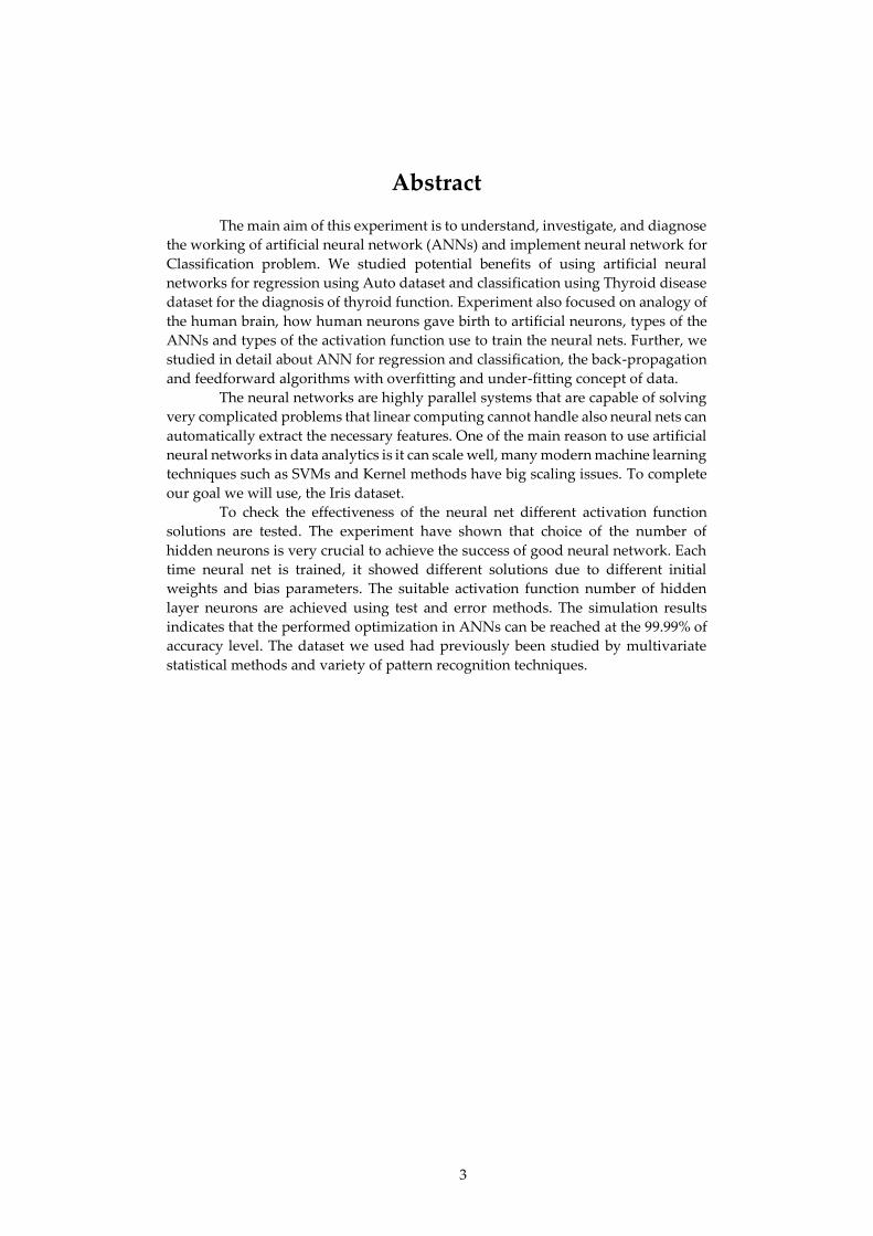
2.4 From Human Neurones to Artificial Neurones
Like the human brain, an artificial neural network is capable of processing
information by connecting together in comparison, simple information processing
units with links that allows each unit to communicate with each other by relatively
simple signals. Every link has a numeric weight associated with it. Weight of links
are the primary means of long-term storage in neural network. Weights are also
updated during the process of learning [3].
𝑥 = {𝑥1, 𝑥2, … , 𝑥𝑁} 𝐼𝑛𝑝𝑢𝑡 𝑉𝑒𝑐𝑡𝑜𝑟
𝑤 = {𝑤1, 𝑤2, … , 𝑤𝑁} 𝑊𝑒𝑖𝑔ℎ𝑡 𝑉𝑒𝑐𝑡𝑜𝑟
𝑛𝑒𝑡 = ∑ 𝑤𝑖𝑥𝑖
𝑁
𝑖=1
𝐴𝑐𝑡𝑖𝑜𝑛 𝑃𝑜𝑡𝑒𝑛𝑡𝑖𝑎𝑙
𝑣 = 𝑛𝑒𝑡 − 𝜃
𝑓(𝑉) 𝐴𝑐𝑡𝑖𝑜𝑛 𝐹𝑢𝑛𝑐𝑡𝑖𝑜𝑛
As can be seen, from the figure an artificial neuron looks almost identical to a human
neuron. Each node has one or more than one inputs, each of them taking values 0 or
1 and single output. Each neuron has several inputs and an output. The neuron has
two modes of operation – the training mode and testing or using mode. In the training
mode, the neuron is trained to respond (weather it should fire or not) to a particular
input of patterns [3]. In the using or testing mode, when a taught pattern is received
as the input to a neuron, its associated output becomes the current output. If the
input pattern does not belongs to the taught list of input patterns, the neuron will
then determine whether it will fire or not. Every input signal has associated weight.
The input information is processed by calculating the weighted sum of the inputs. If
the calculated sum is exceeds a pre-set threshold value, the neuron will fire [3].
Figure 3: Structure of neural net unit (refer from:
http://www.cse.unsw.edu.au/~cs9417ml/MLP2/)

7
The neuron firing mechanism is governed by activation function. The most
common activation functions used are:
2.4.1 Step Function
It is the simplest activation function among all. If xi represents the inputs to a neuron
and wi represents the weights of each edge of all inputs to the node, is [3]:
𝑛𝑒𝑡𝑖 = ∑ 𝑤𝑖𝑥𝑖
The activation function f, is:
𝑓(𝑛𝑒𝑡) = {1 𝑖𝑓 𝑛𝑒𝑡 > 00 𝑖𝑓 𝑛𝑒𝑡 ≤ 0
The graph for step function is:
Figure 4: Step function (taken from- http://www.cse.unsw.edu.au/~cs9417ml/MLP2/)
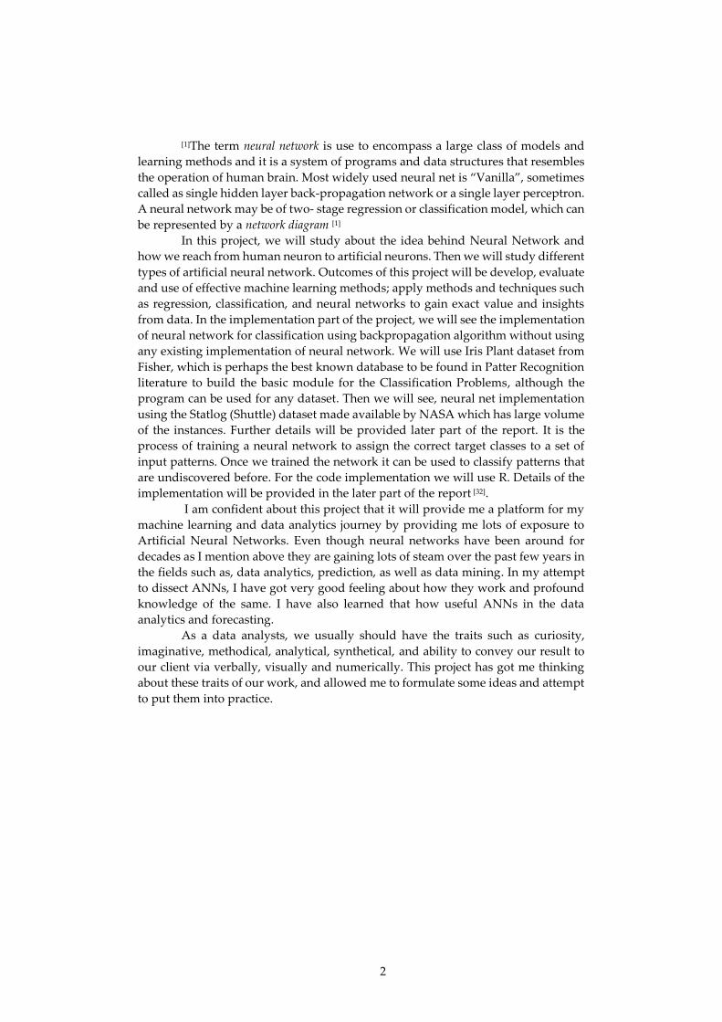
2.4.2 Sigmoid Function
Sigmoid function is non-linear function, unlike the step function, which is linear
function. Here output varies continuously but not linearly as the input changes.
Sigmoid function is best suited for Backpropagation. It is given by the following
expression [3]:
𝑓(𝑛𝑒𝑡) = 1
1 + 𝑒−𝑛𝑒𝑡𝑖
8
The graph for sigmoid function is:
Figure 5: Sigmoid function (taken from- http://www.cse.unsw.edu.au/~cs9417ml/MLP2/)
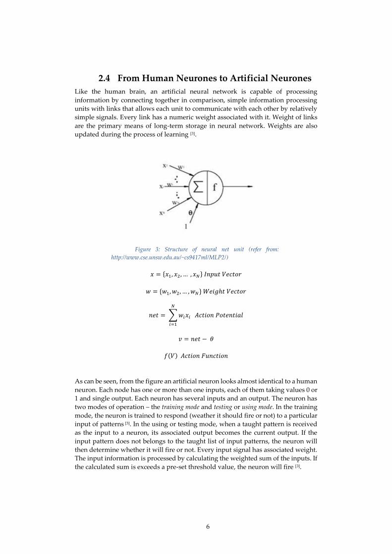
2.4.3 Piecewise Linear Function
Piecewise function is linear function composed of straight-line sections. It is a
piecewise-defined function in which pieces are affine functions. The output is
proportional to the total outputted weight [38]. If piecewise function is continues in
nature, the graph will be a polygonal curve. It is given by the following expression:
𝑓(𝑥) = {
0 𝑖𝑓 𝑥 ≤ 𝑥𝑚𝑖𝑛
𝑚𝑥 + 𝑏 𝑖𝑓 𝑥𝑚𝑎𝑥 > 𝑥 > 𝑥𝑚𝑖𝑛
1 𝑖𝑓 𝑥 ≥ 𝑥𝑚𝑎𝑥
The graph for Piecewise Linear function is:
Figure 6: piecewise linear function (taken from-
http://chronicle.com/blognetwork/castingoutnines/files/2010/01/plcalc3.png)

9
2.4.4 Gaussian Function
Gaussian function has a characteristics symmetric “bell curve” shape that are
continuous. The output of the node (high/low) is interpreted in the class
membership (1/0), it depends on how close the net input is to a chosen value of
average value. It is given by the following expression [38]:
𝑓(𝑥) = 1
√2𝜋𝜎 𝑒
−(𝑥−𝜇)2
2𝜎2
The graph for Gaussian function is:
Figure 7: Gaussian function (taken from-
https://controls.engin.umich.edu/wiki/images/b/ba/Gaussian_Distribution.jpg)
Neural networks can generally categorized in two ways: how the units are connected
and the type of information processed in the unit [3].
The structure for connecting unit can be based on:
Layered Networks: These networks have layered structure of units starting
with an input layer and ending with output layer [3].
Mutually Connected Networks: In this type of network high-order association
is proposed. It has multiple functional modules, each of which is mutually connected
to a neural network with hidden units in order to improve recall performance [3].
2.4.5 Rectified Linear unit
The rectifier activation function allows
a network to easily obtain
sparse representations.

10
2.5 Types of Artificial Neural Networks
There are many types of Artificial Neural Networks. ANNs is emerging
field in computer science and there are many new ANNs are being developed or at
least variations of existing ANNs.
2.5.1 Supervised and unsupervised learning based networks
There are two types of learning methods used in neural network: Supervised and
Unsupervised learning.
2.5.1.1 Supervised Learning
In supervised learning, the concept of teacher is used. The network is
inputted with both input data set and desired (output) data set and thus the teacher
can tell the network when its output is incorrect by showing it what the actual output
should be [17].
2.5.1.2 Self-Organization or Unsupervised Learning
In unsupervised learning, there is no teacher and therefore no rules by
which the network can learn. Here the network is inputted by input data set only.
And, the network finds out some properties and learn it by examining the input data
and ultimately discovering any inherent properties that exists [3]. Depends on the
network model and learning method, network can learn to recognise the exact
properties [17].
2.5.2 Feedback and Feedforward connections based networks
The following list shows some types in each category
2.5.2.1 Unsupervised Learning [17]
Feedback Networks:
Binary Adaptive Resonance Theory (ART1)
Analog Adaptive Resonance Theory (ART2, ART2a)
Discrete Bidirectional Associative Memory (BAM)
Kohonen Self-organizing Map/Topology-preserving map (SOM/TPM)
Discrete Hopfield (DH)
Continuous Hopfield (CH)
Feedforward-only Networks:
Learning Matrix (LM)
Fuzzy Associative Memory (FAM)
Counterprogation (CPN)
Sparse Distributed Associative Memory (SDM)
2.5.2.2 Supervised Learning [17]

11
Feedback Networks:
Brain-State-in-a-Box (BSB)
Fuzzy Congitive Map (FCM)
Boltzmann Machine (BM)
Backpropagation through time (BPTT)
Feedforward-only Networks:
Backpropagation (BP)
General Regression Neural Network (GRNN)
Perceptron
Artmap
Learning Vector Quantization (LVQ)
Probabilistic Neural Network (PNN)
Adaline, Madaline
The following shows some types in details
2.5.3 Feed-Forward Neural Network
This is a simple type of neural network where synapses or connections are initiates
from an input layer to zero or number of hidden layers and ultimately goes to an
output layer. The feed forward neural network is one of the most common and
famous type of neural networks in use, which is suitable for many types of
applications [18]. These networks are often trained using one of the propagation
techniques, via simulated annealing or genetic algorithms. For instance, annealing
is a term used in metallurgy. When any metal is heated to a very high temperature,
it make the atoms moves at high speed. And, when they are cooled very slowly, they
settle into patterns and structures, making the metal much stronger than before. This
principle can be used as an optimization technique in computer science [18].
Simulated annealing basically involves disturbing the independent variables (the
weights of ANN) by a random value and keeping track of the value with the least
error. We can use simulated annealing to aid a neural network and can avoid local
minima scenarios in the energy function [18].
2.5.4 Recurrent Neural Network
Recurrent neural networks (RNNs) are opposite of the Feed-forward networks
which are models with bi-directional data flow. While in feed forward networks
data propagates linearly from input to output, RNNs also propagates it from later
processing stages to earlier stages [16].
2.5.4.1 Hopfield Neural Network
This is simple single layer recurrent neural network. The Hopfield neural network
is trained using an algorithm which teaches the network to learn to recognise
patterns and it requires stationary inputs [18]. The Hopfield network will indicate that

12
the pattern is recognized by echoing it back. This type of neural networks are
typically used for pattern recognition. It is invented by John Hopfield in 1982 [18].
2.5.4.2 Simple Recurrent Network (SRN) - Elman or Jordan Style
This is a simple recurrent neural network that has three-layers with the additional
set of a “context units” which are situated at the input layer [18]. The context unit
stores the previous output values of the hidden layer and then echoes back the
values to hidden layer’s input. Thus hidden layer always inputted with values from
its previous iteration's output values. Elman or Jordan neural networks are typically
used for prediction problems [18]. Elman or Jordan neural networks are generally
trained by using genetic, simulated annealing, or one of the propagation techniques
[18].
2.5.4.3 Bi-directional RNN
Bi-directional RNNs, or BRNNs are invented by Schuster & Paliwal in 1997. BRNNs
use a finite sequence to predict or label each element of the sequence based on both
the past and the future context of the element [16]. The BRNNs works by adding the
outputs of two RNNs – among which one start processing the sequence from right
to left, the other one from left to right. The outputs are combined and uses the
predictions of the teacher-given target signals. This technique is especially useful
when combined with LSTM RNNs [16].
2.5.5 Radial Basis Function (RBF) Network
Radial basis function network is a feed forward network with an input layer, hidden
layer and a summation layer or output layer. The hidden layer is based on a radial
basis function which is powerful technique for interpolation in multidimensional
space. Radial basis functions have been applied in the area of neural networks where
they may be used as a replacement for the sigmoidal hidden layer transfer
characteristic in multi-layer perceptron [16]. Different types of radial basis functions
can be used but the Gaussian function is generally employed in RBF. Some RBF's in
the hidden layer can be used to approximate more complex activation function than
a typical feed forward neural network. RBF networks are typically used for pattern
recognition [18]. They can be trained via annealing, genetic or via one of the
propagation techniques. RBF networks the same advantage of not suffering from
local minima as a Multi-Layer perceptron. It can be possible because the linear
mapping from hidden layer to output layer is the only parameter that is adjusted in
the learning process [18].
2.5.6 Radial Basis Function (RBF) Network
According to biological studies, the human brain does not as a single massive
network, but it has a small networks which works separately [18]. This understanding
gave birth to the concept of Modular Neural Networks, where several small
networks work together to solve the complicated problems [18].

13
2.6 Neural Network Theory
Simple Linear Regression:
To predict scores on one variable from the scores on another variable is called as
Simple Linear Regression. The variable we are predicting is called the criterion
variable and is called as Y. The variable from which our predictions are based are
called the predictor variable and is referred to as X [34]. When there is only single
predictor variable, the prediction method is called simple regression. In simple
linear regression, the predictions of Y when plotted as a function of X forms a
straight line. We just have one attribute in simple linear repression and parameters
are vectors (𝛽0
𝛽1) ∈ ℝ2 and learning machine is [37]:
𝐹(𝑥, 𝛽) = 𝛽0 + 𝛽1𝑥
Multiple Linear Regression:
The extension to multiple and/or vector-valued predictor variables (which is
denoted by capital X) is known as multiple linear regression, also known as
multivariable linear regression. However in this case y which is response variable
still a scalar [34]. Here we have p – whereas p > 1 – attributes [37]. We use a linear
function for prediction. In case of multiple linear regression parameters are vectors
(𝛽0
, 𝛽1
, … , , 𝛽𝑝) ∈ ℝ𝑝+1 and the learning machine is as follows [37]:
𝐹(𝑥, 𝛽) = 𝛽0 + 𝛽1𝛽𝑥1 + ⋯ + 𝛽𝑝𝑥𝑝
Logistic Regression:
Logistic regression can be considered the classification counterpart of linear
regression. It is useful because it can accept an input with any value from negative
to positive infinity, whereas the output values are always between zero and one [35].
The default label falls into one of two categories, which is Yes or No. Rather than
modelling this label Y directly, logistic regression models the probability that Y is
Yes. Which let us encode Yes as 1 and No as 0. Namely, logistic regression models
𝑝(𝑋) = ℙ(𝑌 = 1|𝑋) where 𝑋 = (𝑋1 … 𝑋𝑝)′ by [37]
𝑝(𝑋) = 𝜎(𝛽0 + 𝛽1𝑋1 + ⋯ + 𝛽𝑝𝑋𝑝
Where, 𝜎 is the logistic function, (Which is called as sigmoid function in the
context of Neural Networks) and it is define as follows [37]:
𝜎(𝑥) =1
1 + 𝑒−𝑥=
𝑒𝑥
1 + 𝑒𝑥

14
[1]The term neural network is use to encompass a large class of models and
learning methods and it is a system of programs and data structures that resembles
the operation of human brain. Most widely used neural net is “Vanilla”, sometimes
called as single hidden layer back-propagation network or a single layer perceptron.
A neural network may be of two- stage regression or classification model, which can
be represented by a network diagram [1] [37]
[1] [37]For each neurons contained in the particular neural network there are
following
- k weights w1, w2, …, wk where k is the number of arrows that entering into
that neuron.
- b is one threshold.
If neuron receives the signal s1, s2,…, skfrom the input variables below it, it
sends the signal to the neurons above it
- θ(w1s1 + w2s2 + … + wksk - b)
θ is a step function or activation function
- θ(t) = 1 if t > 0
- θ(t) = 0 otherwise
The way neural net functions is as follows
- The input variables send their values to the level 1 neurons above them.
- Level 1 neurons compute their output by the formula θ (w1s1 + w2s2 + · · · +
wksk − b) and send it to the next level i.e. level 2 neurons above them.
- The output neurons compute their outputs, and the vector of outputs is the
overall output of the net [37][01].
Training a neural network includes of setting the weights and thresholds for
all the neurons and possibly changing the topology of the network. A parameter
consists of all weights and thresholds and the topology if it is variable [01].
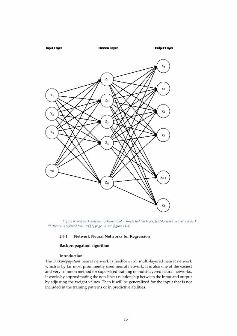
- At the bottom of the diagram we have our standard input variables
(attributes) X1, X2, X3, .., Xp
- In the middle of the diagram we have hidden layer consists of the units
(not quiet neurons) Z1, Z2, Z3,.., Zm.
- On top the output nodes are Y1, Y2, .., Yk for simplicity, let’s consider K = 1
and write Y for Y1 [01].
15
2.6.1 Network Neural Networks for Regression
Backpropagation algorithm
Introduction
The Backpropagation neural network is feedforward, multi-layered neural network
which is by far most prominently used neural network. It is also one of the easiest
and very common method for supervised training of multi-layered neural networks.
It works by approximating the non-linear relationship between the input and output
by adjusting the weight values. Then it will be generalized for the input that is not
included in the training patterns or in predictive abilities.
Figure 8: Network diagram Schematic of a single hidden layer, feed-forward neural network [1] (figure is referred from ref [1] page no 393 figure 11.3)

16
In general Backpropagation network has two stages, first training and
second is testing. While performing training phase, network is shown simple inputs
and correct classifications. For example, the input might be encoded picture of face,
and the output could be corresponds as the person name. Like most learning
algorithms, neural network needs to have inputs and outputs according to an
arbitrary user defined scheme. The scheme is used to create the network architecture
so as soon as network is trained, the scheme cannot be changed without creating a
total new net. There are lots of forms to encode the response of network [3].
The figure shows the topology of the Backpropagation neural network that
includes an input layer which accepts number of inputs, one hidden layer and an
output layer. Backpropagation neural network can have more than one hidden
layers [3].
Theory
The Backpropagation neural network operation are divided into two steps
feedforward and backpropagation. In the feedforward steps, an input pattern is
applied to the input layer and its effects propagates, layer by layer, through the all
layers include hidden layer until an output is produced. The actual value of network
is then compared to the expected output, and the error signal is computed for each
of the output node [3]. Since all the hidden nodes within network have, to some
degree, contributed to the errors evident in the output layer, then the output error
signals are transmitted backward from the output layer to each node in the hidden
layer that immediately contributed the output layer. This process is then repeated,
layer to layer, until each and every node in the network has received an error signal
that describes its relative contribution to the overall error. After the error signal for
each node has been determined, the error calculated are used by nodes to update
each connection weights until the network meets to the state which allows all the
training patters to be encoded [3].
The backpropagation algorithm looks for the minimum error function value
in weight space. This is accomplished by using technique called delta rule or gradient
Figure 9: Backpropagation Neural Network with one hidden layer (source-figure is taken
from http://www.cse.unsw.edu.au/~cs9417ml/MLP2/)

17
decent. The weights that minimize the error function is then considered to be a
solution to the learning problem. The behaviour of the network is analogous to a
human that is shown a set of data and is asked them to classify into prediction classes [3].
Over-fitting, Under-fitting and Model Complexity
Neural networks are often referenced as universal function which approximates
since theoretically any continuous function can be approximated to a prescribed
degree of accuracy by increasing the number of neurons in the hidden layer of a
feedforward backpropagation network [11]. This can be proven by Kolmogrov's
theorem stating that a neural network with linear n (2n+1) combinations of
monotonically increasing nonlinear functions of only one variable is able to fit any
continuous function of n variables [12]. Yet in reality, the objective of a multivariate
calibration is not to approximate a calibration data set with an ultimate accuracy,
but to find a calibration with the best possible generalizing ability [13]. This gap
between the approximation of a calibration data set and the generalization ability of
a calibration becomes the more problematic the higher the number of variables and
the smaller the data set. The complexity of neural networks can be mainly reduced
to the number of adjustable parameters, such as the number of biases and the
number of weights. Although the number of hidden layers also seems to influence
the complexity of the neural networks [10] [8].
There are some issues also related to generalizing a neural network. Issues
to consider are problems related to over-fitting of training data and under-fitting of
training data [10] [8].
Under-Fitting of training data
Under-training can occur when the neural network is not complex enough to detect
the pattern in the complicated data set. This type of issue usually the result of
networks with very few hidden nodes that it cannot accurately represents the
expected solutions, therefore under-fitting the data.
To prevent under-fitting of data we need to make sure that, the network has
enough hidden units to represent the required mappings and it is trained for long
enough that the error/cost function (e.g., SSE or Cross Entropy) is sufficiently
minimised [14].

18
Over-Fitting of training data
Over-fitting can be observed in a network that is very complex, which results in
predictions that are far beyond the range of the training data. This is usually the
result of networks with too many hidden layers, therefore over-fitting the data [3].
To prevent the over-fitting we have several options like, we can stop the
training early before it has had time to learn the training data very well, we can add
Figure 10: Under-Fitting of training data (source-taken from
http://www.cse.unsw.edu.au/~cs9417ml/MLP2/)
Figure 11: Over-Fitting of training data (source- taken from
http://www.cse.unsw.edu.au/~cs9417ml/MLP2/)

19
noise to the training patters to clean out the data points, we can add some form of
regularization term to the error/cost function to encourage smoother network
mappings and we can restrict the number of adjustable parameter the network has
for e.g. we can reduce number of hidden units, or we can force connections to share
the same weight values[14] [3].
The aim is to create a neural network with the exact number of hidden nodes
that will lead to a good solution to the problem [3].
Using figure, the following describes the learning algorithms used and the
equations used to train a neural network [3].
Feedforward Algorithm [3]When a specified training pattern is fed to the input layer, the weighted sum of the
input to the jth node in the hidden layer is given by:
Netj = ∑ wij xj + øj (1) Above equation is used to calculate the neuron’s aggregated input.
Weighted value is term øj and it is from a bias node that has an output value of 1.
The bias node is Pseudo Input to each neuron in the hidden and output layer, and
also to solve the problems which are related with the situation where values of input
patter is 0, we can use bias node. If any of the input pattern has 0 values, the neural
network could not be trained without a bias node [3].
The "Net" term, also known as the action potential, is passed onto an
appropriate activation function, which decide whether a neuron should fire or not.
The resulting value of the activation function determines the neuron's output, and
becomes the input value for the neurons in the next layer connected to it.
Backpropagation algorithm has different requirements and one of them is that the
activation function should be differentiable, a one of the well-known activation
function used is the sigmoid equation which is given by the following equation [3]:
Figure 12: Good fit of the training data (source-
http://www.cse.unsw.edu.au/~cs9417ml/MLP2/)
20
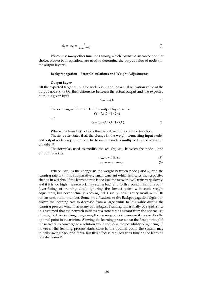
𝑂𝑗 = 𝑥𝑘 = 1
1+ 𝑒−𝑁𝑒𝑡𝑗
(2)
We can use many other functions among which hyperbolic tan can be popular
choice. Above both equations are used to determine the output value of node k in
the output layer [3].
Backpropagation – Error Calculations and Weight Adjustments
Output Layer [3]If the expected target output for node k is tk, and the actual activation value of the
output node k, is Ok, then difference between the actual output and the expected
output is given by [3]:
∆k = tk - Ok (3)
The error signal for node k in the output layer can be:
∂k = ∆k Ok (1 - Ok)
Or
∂k = (tk - Ok) Ok (1 - Ok) (4)
Where, the term Ok (1 - Ok) is the derivative of the sigmoid function.
The delta rule states that, the change in the weight connecting input node j
and output node k is proportional to the error at node k multiplied by the activation
of node j [3].
The formulas used to modify the weight, wj,k, between the node j, and
output node k is:
∆wj,k = ℓr ∂k xk (5)
wj,k = wj,k + ∆wj,k (6)
Where, ∆wi,j is the change in the weight between node j and k, and the
learning rate is ℓr. ℓr is comparatively small constant which indicates the respective
change in weights. If the learning rate is too low the network will train very slowly,
and if it is too high, the network may swing back and forth around minimum point
(over-fitting of training data), ignoring the lowest point with each weight
adjustment, but never actually reaching it [3]. Usually the ℓr is very small, with 0.01
not an uncommon number. Some modifications to the Backpropagation algorithm
allows the learning rate to decrease from a large value to low value during the
learning process which has many advantages. Training will initially be rapid, since
it is assumed that the network initiates at a state that is distant from the optimal set
of weights [3]. As learning progresses, the learning rate decreases as it approaches the
optimal point in the minima. Slowing the learning process near the first point uplift
the network to converge to a solution while reducing the possibility of ignoring. If,
however, the learning process starts close to the optimal point, the system may
initially swing back and forth, but this effect is reduced with time as the learning
rate decreases [3].

21
In equation (5), the xk variable is the input value to the node k, and is the
same value as the output from node j [3].
To improve the process of updating the weights, equation (5) is modified to:
∆wj,kn = ℓr ∂k xk + ∆wj,k(n - 1) µ (7)
[3]Here the updating of weight during the nth iteration is determined by
including a momentum term (µ), which is multiplied to the (n - 1)th iteration of the
∆wj,k. The momentum term is used to accelerate the learning process by
"encouraging" the weight changes to continue in the same direction with larger steps
[3]. Also, the momentum term prevents the learning process from fixing in a local
minimum by "over stepping" the small "hill". Typically, the momentum term has a
value between 0 and 1 [3].
Hidden Layer
The error signal for node j in the hidden layer can be calculated by [3]:
∂k = (tk – Ok) Ok ∑(wj,k ∂k) (8)
Where, the sum term adds the weighted error signal for all nodes k, in the output
layer.
As before, to adjust the weight wi,j, between the input node i, and the node j formula
is [3]:
∆wi,jn = ℓr ∂j xj + ∆wi,j(n - 1) µ (9)
wi,j = wi,j + ∆wi,j (10)
Figure 13: Global and Local Minima of Error Function [3] (figure is taken from
http://www.cse.unsw.edu.au/~cs9417ml/MLP2/)

22
Global Error
Backpropagation is derived by concluding that it is useful to minimize the error on
the output nodes over all the patterns presented to the neural network. The error
function E for all patterns, calculated by following equation [3],
E = ½∑ (∑ ( tk – Ok )2 ) (11) [1] [37]The neural network model has unknown parameters, often called weights, and
we finds out values for them that make the model fit the training data well. We
denote the complete set of weights by λ, which consists of [37]
{αm,0 and αm,l for m = 1,...,M} and ℓ = 1,...,p weights
{β0 and βm for m = 1,...,M} weights
αm,0 and β0 play the role of thresholds
there are M(p + 1) + (M + 1) weights overall
convenient notations are
αm = (αm,1,...,αm,p)’ β = (β1,...,βM)’
X = (X1,...,Xp)’ Z = (Z1,...,ZM)’
Details of regression neural net – the learning machine works as follows
Zm = σ (αm0 + α’mX), m = 1, . . . , M,
Y = β0 + β’Z
Role of σ is
Without σ, it would have been just linear regression [37]
With σ, the prediction rules that we can get are sophisticated non-linear
functions [37].
For regression, we will use sum-of-squared errors as our measure of fit
(error function)
𝑅(𝜃) = ∑
𝐾
𝑘=1
∑(𝑦𝑖,𝑘 − 𝑓𝑘 (𝑥𝑖))2
𝑁
𝑖=1
For classification, we will use either squared error or cross-entropy
(deviance)
𝑅(𝜃) = − ∑
𝐾
𝑘=1
∑ 𝑦𝑖,𝑘 𝑙𝑜𝑔 𝑓𝑘 (𝑥𝑖)
𝑁
𝑖=1
[1] [37] In the cases where neural networks do not work well, we always have
a failure of the learning algorithm (such as back-propagation) to find the right M or
weights. We do not really want to use the ERM principle because, minimizing the
training error is not computationally feasible and even if it were, we could over-fit.
Instead we do something similar like, slowly move against the gradient of the

23
training MSE until some stopping condition is met [37]. Namely: at each step we add
− η times the gradient, where η (the learning rate) is a small positive constant. To
compute the gradient, as usual, we can use training set (x1, y1)…., (xn, yn); it is fixed.
The training MSE is
1
𝑛 ∑ 𝑅𝑖 𝑤ℎ𝑒𝑟𝑒 𝑅𝑖 = (𝑦𝑖 − 𝑌𝑖)2
𝑛
𝑖=1
For given parameters, we can compute the values of the nodes Zm and Y for
each observation i= 1…n; we will denote them as Zim and Yi, respectively. And will
set xi0 = 1 and Zi0 = 1 for all observations [37]. The standard rules gives:
𝜕𝑅𝑖
𝜕𝛽𝑚
= −2 (𝑦𝑖 − 𝑌𝑖)
𝜕𝑌𝑖
𝜕𝛽𝑚
= −2 (𝑦𝑖 − 𝑌𝑖)𝑍𝑖𝑚
And
𝝏𝑹𝒊
𝝏𝜶𝒎𝓵= −𝟐 (𝒚𝒊 − 𝒀𝒊)
𝝏𝒀𝒊
𝝏𝜶𝒎= −𝟐 (𝒚𝒊 − 𝒀𝒊)𝜷𝒎
𝝏𝒁𝒊𝒎
𝝏𝜶𝒎𝓵= −𝟐 (𝒚𝒊 − 𝒀𝒊)𝜷𝒎𝝈′(𝜶𝒎𝟎 + 𝜶′𝒎𝒙𝒊)𝒙𝒊𝓵
Where, m = 0 is allowed in βm and ℓ = 0 is allowed in αmℓ [37].
A nicer representation of above observations, by rewriting the derivatives
as 𝜕𝑅𝑖
𝜕𝛽𝑚
= −𝜕𝑖𝑍𝑖𝑚
𝜕𝑅𝑖
𝜕𝛼𝑚
= −𝑠𝑖𝑚𝑥𝑖𝑙
Where the “errors” ∂ and s are defined by
𝜕𝑖 = 2 (𝑦𝑖 − 𝑌𝑖)
𝑠𝑖𝑚 = 𝛽𝑚𝜎′(𝛼𝑚0 + 𝛼′𝑚𝑥𝑖)𝜕𝑖
Also called as the backpropagation equations [37].
The overall gradient of the training MSE is given by the following equations
𝜕𝑀𝑆𝐸
𝜕𝛽𝑚
= −1
𝑛∑
𝑛
𝑖=1
𝜕𝑖𝑍𝑖𝑚
And

24
𝜕𝑀𝑆𝐸
𝜕𝛼𝑚ℓ
= −1
𝑛∑
𝑛
𝑖=1
𝑠𝑖𝑚𝑥𝑖ℓ
The Backpropagation Algorithm [37] [1]Start from random weights βm and αmℓ. Repeat the following for a number of
epochs (or until a stopping condition is satisfied). For each training observation (i =
1,..., n) do the following [37].
1. Forward pass:
Compute the variables Zm and Y for the ith training object xi.
The learning machine works as follows:
Zm = σ (αm0 + α’mX) m = 1, . . . , M,
Y = β0 + β’Z.
The role of σ
• Without σ, it would have been just linear regression!
• With σ, the prediction rules that we can get are sophisticated
non-linear functions.
2. Backward pass:
Compute the “error”
δ = 2(yi − Y)
and back-propagate it to
sim = δβmσ ‘(αm0 + α’m xi)
Update the weights:
𝛽𝑚 = 𝛽𝑚 + η
𝑛 𝛿𝑚
𝛼𝑚ℓ = 𝛼mℓ +η
𝑛𝑠𝑚𝑥𝑖ℓ
Differentiating the sigmoid function, following expression is for σ’
σ’(x) = 𝑒𝑥
(𝑒𝑥 + 1)2
Inputs of the neural network should be scaled it is important for the neural
networks. Trevor Hastie’s advice: “standardize all attributes to have mean 0 and
standard deviation 1”. The starting weights are usually chosen as a random numbers
around 0 because, with standardized inputs, it is typical to take the starting weights
distributed uniformly on [-0.7, 0.7] [37]. Starting with large weights generally leads to
poor solutions. The objective function (i.e. the training MSE as the function of the
25
weights) is not convex, and there can be multiple minima. It is easy to get stuck in
one. To prevent this, run the algorithm several times with different starting weights.
Possibilities to decide when to stop [37]
First possibility to decide when should stop, we can divide the available data into a
two parts a training set and a validation set and train the neural network on the
training set until the error (such as MSE) on the validation set starts increasing.
Finally train the neural network on all data using the number of epochs giving the
minimal error on the validation set. But this has one disadvantage, a significant
fraction of the available data is not used for training [37].
Another possibility to decide when should stop, we can use cross- validation; steps
involves in cross-validation are [37]
- Divide the available data into K (such as K = 10) folds.
- For each k = 1,..., K: Train the neural network on all data except for fold k;
let epk be the epoch at which the best error on fold k is attained.
- Find the average 𝑒𝑝̅̅ ̅ = 1
𝐾 ∑ 𝑒𝑝𝑘𝑘𝑘=1
- Train the neural network on all available data for 𝑒𝑝̅̅ ̅ epochs
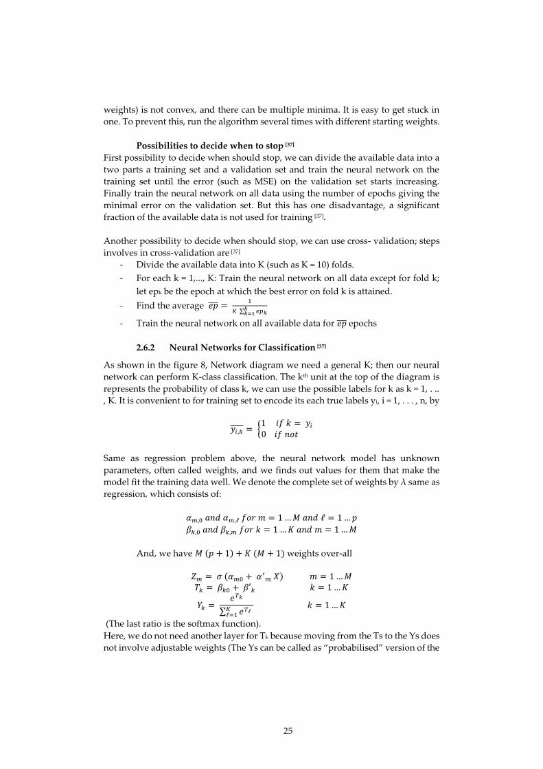
2.6.2 Neural Networks for Classification [37] As shown in the figure 8, Network diagram we need a general K; then our neural
network can perform K-class classification. The kth unit at the top of the diagram is
represents the probability of class k, we can use the possible labels for k as k = 1, . ..
, K. It is convenient to for training set to encode its each true labels yi, i = 1, . . . , n, by
𝑦𝑖,𝑘 = {1 𝑖𝑓 𝑘 = 𝑦𝑖
0 𝑖𝑓 𝑛𝑜𝑡
Same as regression problem above, the neural network model has unknown
parameters, often called weights, and we finds out values for them that make the
model fit the training data well. We denote the complete set of weights by λ same as
regression, which consists of:
𝛼𝑚,0 𝑎𝑛𝑑 𝛼𝑚,ℓ 𝑓𝑜𝑟 𝑚 = 1 … 𝑀 𝑎𝑛𝑑 ℓ = 1 … 𝑝
𝛽𝑘,0 𝑎𝑛𝑑 𝛽𝑘,𝑚 𝑓𝑜𝑟 𝑘 = 1 … 𝐾 𝑎𝑛𝑑 𝑚 = 1 … 𝑀
And, we have 𝑀 (𝑝 + 1) + 𝐾 (𝑀 + 1) weights over-all
𝑍𝑚 = 𝜎 (𝛼𝑚0 + 𝛼′
𝑚 𝑋) 𝑚 = 1 … 𝑀 𝑇𝑘 = 𝛽𝑘0 + 𝛽′𝑘 𝑘 = 1 … 𝐾
𝑌𝑘 = 𝑒𝑇𝑘
∑ 𝑒𝑇ℓ𝐾ℓ=1
𝑘 = 1 … 𝐾
(The last ratio is the softmax function).
Here, we do not need another layer for Tk because moving from the Ts to the Ys does
not involve adjustable weights (The Ys can be called as “probabilised” version of the
26
Ts.) [37]. We will be using this softmax function in our neural network
implementation described in later part of the coding for loss function.
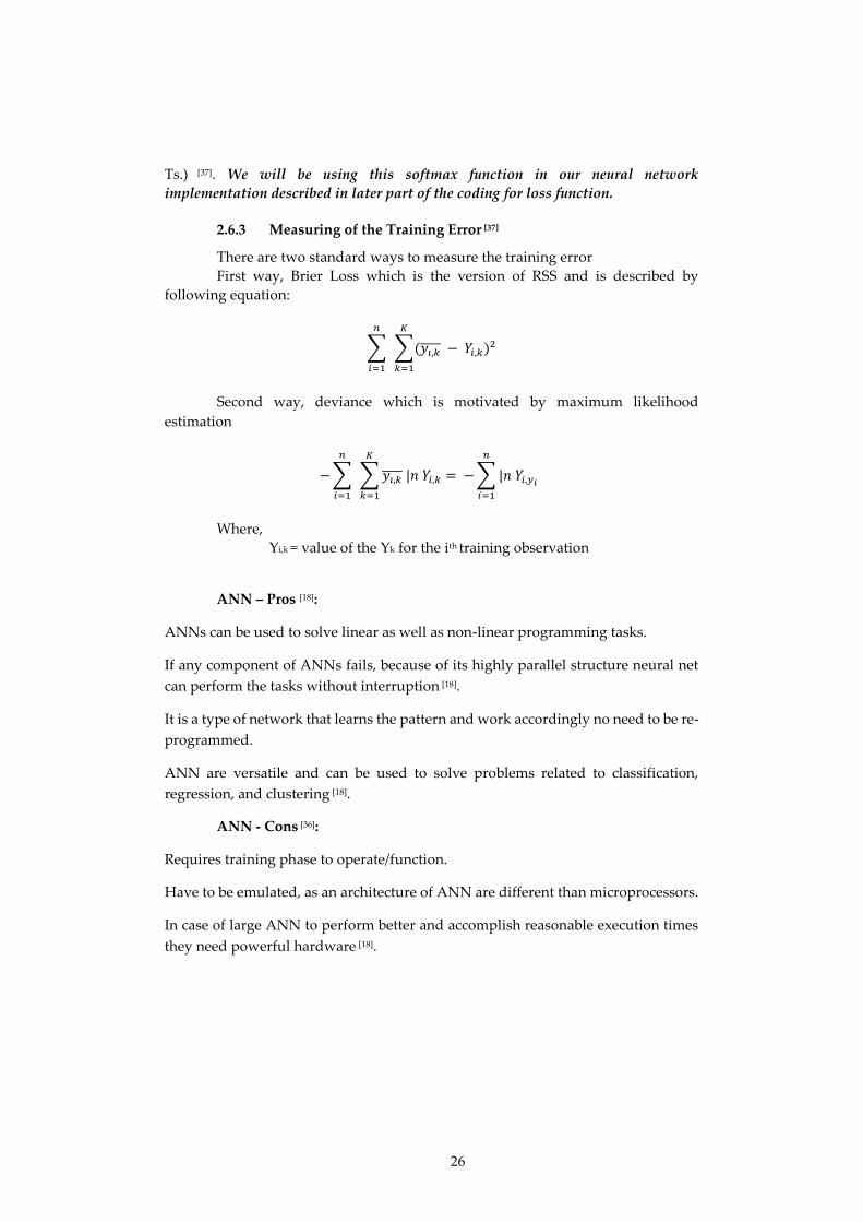
2.6.3 Measuring of the Training Error [37]
There are two standard ways to measure the training error
First way, Brier Loss which is the version of RSS and is described by
following equation:
∑
𝑛
𝑖=1
∑(𝑦𝑖,𝑘̅̅ ̅̅ − 𝑌𝑖,𝑘)2
𝐾
𝑘=1
Second way, deviance which is motivated by maximum likelihood
estimation
− ∑
𝑛
𝑖=1
∑ 𝑦𝑖,𝑘̅̅ ̅̅ |𝑛 𝑌𝑖,𝑘 = − ∑ |𝑛 𝑌𝑖,𝑦𝑖
𝑛
𝑖=1
𝐾
𝑘=1
Where,
Yi,k = value of the Yk for the ith training observation
ANN – Pros [18]:
ANNs can be used to solve linear as well as non-linear programming tasks.
If any component of ANNs fails, because of its highly parallel structure neural net
can perform the tasks without interruption [18].
It is a type of network that learns the pattern and work accordingly no need to be re-
programmed.
ANN are versatile and can be used to solve problems related to classification,
regression, and clustering [18].
ANN - Cons [36]:
Requires training phase to operate/function.
Have to be emulated, as an architecture of ANN are different than microprocessors.
In case of large ANN to perform better and accomplish reasonable execution times
they need powerful hardware [18].

27
3 Experiment
3.1 Task
Neural networks are class of learning methods that was developed in two different
fields – statistics and artificial intelligence – they are based on essentially identical
models. Neural networks are just nonlinear statistical models much like the
projection pursuit models. A neural network is two-stage regression or classification
model. The goal of the experiment is to implement the neural network for
classification. To this end, we focussed on the following areas:
- Implement neural network for Classification using back-propagation
algorithm for Iris dataset without using any existing implementations.
- Implement neural network for Classification using back-propagation
algorithm for Statlog (Shuttle) dataset without using any existing
implementations.
- Compare the neural network with Decision Tree Algorithm.
3.2 Preparatory Work
3.2.1 Exploration
The neural net back-propagation algorithm allows multilayer feed-forward neural
networks to learn input/output mappings using training samples of the dataset [41].
Back-propagation algorithm has functionality to adapt itself to learn the relationship
between the set of example patterns, and could be able to apply the same
relationship to the new input patterns which also makes it fast algorithm for
learning. It actually allows us to see detailed insights onto how changing the biases
and weights changes the overall behaviour of the given network [41]. The activation
function is used to transform the activation level of a unit (neuron) into an output
signal [41]. There are a numerous activation functions in use with artificial neural
network. One of the core purpose of the project is to perform analysis using some of
these different activation functions to figure out the optimal activation function for
a problem and provide a benchmark of it [41].
With the aim of finding optimal activation function in problem and classify patterns
in the data, I explore several possibilities. The options include decision trees, SVM
etc. but decision trees tend to overt noisy data and are not as intuitive as some other
classification methods available [40]. Whereas, artificial neural networks can model
more arbitrary functions (nonlinear interactions etc.) and can handle binary data
better than decision trees, it is best for time series based learning [40]. Also neural
networks scales well using techniques such as stochastic gradient descent that can
deal with huge databases because many more modern machine learning techniques
such as SVMs and other Kernel methods have big scaling issues.

28
3.2.2 Knowledge Acquisition
To get the deep knowledge of neural network I went through the book on “An
Introduction to Neural Networks, James A Anderson, MIT Press, 1995”. Further I
tried to get as much as information on neural network for regression and
classification. The book “The Elements of Statistical Learning (Second edition,
Springer, 2009) by T. Hastie, R. Tibshirani, and J. Friedman” was the best choice for
me to get profound knowledge for my project. I wrote my own code in R for
classification using neural network.
Choice of Programming Language
I used R which is also called as GNU S. It is a strongly functional language and
environment for statistical computing and graphics. Which was fair choice for this
implementation as it is freely available and open source. I used R for implementation
of Classification problem.
3.2.3 Datasets Used
The main aim of the thesis was, to build the proper classification neural network
module which can be easily modifiable for adaptation of different database. By
keeping this in mind I chose Iris Plants dataset which is very small dataset but it was
ideal dataset for the purpose. For the main purpose I chose 2 datasets both are
classification problem datasets. First one is Starlog (Shuttle) dataset and second one
is Iris plant dataset both are available on UCI Machine Learning Repository. The
details of the dataset as follows.
Iris Plants Data Set [39]
The dataset is made available by R.A. Fisher. This is perhaps the best known
database to be found in the pattern recognition literature. Fisher's paper is a classic
in the field and is referenced frequently to this day. The data set contains 3 classes
of 50 instances each, where each class refers to a type of iris plant. One class is
linearly separable from the other 2; the latter are NOT linearly separable from each
other [39].The characteristics of the dataset is Multivariate and all the attributes are
Real. The dataset belongs to Life area.
Format:
A data frame has 4 attributes and 150 number of instances. The details of the
attributes are as follows:
1. sepal length in cm
2. sepal width in cm
3. petal length in cm
4. petal width in cm
5. classes :
-- Iris Setosa
-- Iris Versicolour
-- Iris Virginica
There are no missing values in the dataset [39].

29
Statlog (Shuttle) Data Set [31]
The dataset is made available by Jason Catlett of Basser Department of Computer
Science, University of Sydney, N.S.W. with the help of NASA. Approximately 80%
of the data belongs to class 1. Therefore the default accuracy is about 80%. The aim
here is to obtain an accuracy of 99 - 99.9% [31]. The examples in the original dataset
were in time order, and this time order could presumably be relevant in
classification. However, this was not deemed relevant for StatLog purposes, so the
order of the examples in the original dataset was randomised, and a portion of the
original dataset removed for validation purposes [31]. The characteristics of the
dataset is Multivariate and all the attributes are Integers. The dataset belongs to
physical area [31].
Format:
A data frame has 9 attributes and 58000 number of instances, which makes
it large dataset and deal enough for the thesis. Amongst the 9 attributes first one
being time and the last column is the class which has be coded as follows:
1. Rad Flow
2. Fpv Close
3. Fpv Open
4. High
5. Bypass
6. Bpv Close
7. Bpv Open
There are no missing values in the dataset [31].
3.3 Approach
3.3.1 For Satlog (Shuttle) Data Set
Phase 1: Defining the problem
The diagram below is for Statlog (Shuttle) dataset. Which shows the working of the
purposed neural network. Input features are the 9 attributes as inputs to the
network. The neural network used 10 default hidden layers to capture potential
patterns within the network. Number of hidden layers can be changed accordingly.
The possible output for the categories of classification has 2 output classes.

30
Phase 2: Defining function for prediction for the neural network
The following code function will be used for neural net prediction
> neural_net_predict <- function(model, data = X.test)
This function will accept model and data set as an argument.
# function arguments
# trained_model - trained model from neural network training
# data - test data
Phase 3: Defining function for training of the neural network
The following code function will be used for neural net training
> neural_net_train <- function(x, y, traindata=data, testdata=NULL,
trained_model = NULL,
number_hidden_neurons=c(6),
Figure 14 Neural network for Statlog(Shuttle) dataset

31
no_of_epochs=2000,
loss_fuc=1e-2,
learning_rate = 1e-2,
reg_rate = 1e-3,
display = 100,
random.seed = 1,
activation_function = 'relu')
This function will accept model, training data, testing data, number of hidden
neurons, number of hidden neurons, learning rate and some default arguments.
# function arguments
#
# x - attributes
# y - labels
# traindata - training subset
# testdata - testing subset
# trained_model - return value
# number_hidden_neurons - number of hidden neurons
# no_of_epochs - number of epochs
# display - display interval
# random.seed - seed value
# activation_function - activation function
# loss_fuc - delta loss = softmax
# learning_rate - learning rate
# reg_rate - regularization rate
Phase 4: Applying Activation Function.
Activations function can apply for datasets.
>hidden_layer <- pmax(hidden_layer, 0)
Above code will be used for Rectified Linear function.
Phase 5: Defining function for testing of the neural network.
The following function call will be used for the training purpose of the neural
network model.
> neural_net_iris_test <- function(dataset_name, attr, lbl, actfun, num_itr, hnrs,
include_test)
# function arguments
#
# dataset_name - dataset for neural net classification
# attr - features of dataset
# lbl - label / class to be learned and predicted
# actfun - activation function
# num_itr - epochs
32
# hnrs - number of hidden neurons
# include_test - indicator for running train + test (Y) OR just train (N)
3.3.2 For Iris Data Set
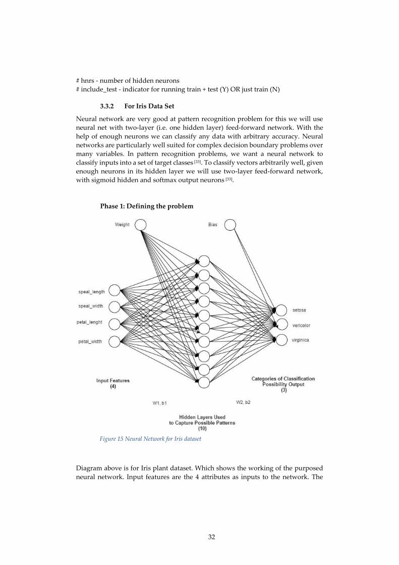
Neural network are very good at pattern recognition problem for this we will use
neural net with two-layer (i.e. one hidden layer) feed-forward network. With the
help of enough neurons we can classify any data with arbitrary accuracy. Neural
networks are particularly well suited for complex decision boundary problems over
many variables. In pattern recognition problems, we want a neural network to
classify inputs into a set of target classes [33]. To classify vectors arbitrarily well, given
enough neurons in its hidden layer we will use two-layer feed-forward network,
with sigmoid hidden and softmax output neurons [33].
Phase 1: Defining the problem
Diagram above is for Iris plant dataset. Which shows the working of the purposed
neural network. Input features are the 4 attributes as inputs to the network. The
Figure 15 Neural Network for Iris dataset

33
neural network used 10 default hidden layers to capture potential patterns within
the network. Number of hidden layers can be changed accordingly. The possible
output for the categories of classification has 3 output classes.
Phase 2: Defining function for prediction for the neural network
The following code function will be used for neural net prediction
>neural_net_predict <- function(model, data = X.test)
This function will accept model and data set as an argument.
# function arguments
# trained_model - trained model from neural network training
# data - test data
Phase 3: Defining function for training of the neural network
The following code function will be used for neural net training
> neural_net_train <- function(x, y, traindata=data, testdata=NULL,
trained_model = NULL,
number_hidden_neurons=c(6),
no_of_epochs=2000,
loss_fuc=1e-2,
learning_rate = 1e-2,
reg_rate = 1e-3,
display = 100,
random.seed = 1,
activation_function = 'relu')
This function will accept model, training data, testing data, number of hidden
neurons, number of hidden neurons, learning rate and some default arguments.
# function arguments
#
# x - attributes
# y - labels
# traindata - training subset
# testdata - testing subset
# trained_model - return value
# number_hidden_neurons - number of hidden neurons
# no_of_epochs - number of epochs
# display - display interval
# random.seed - seed value
# activation_function - activation function
# loss_fuc - delta loss = softmax
# learning_rate - learning rate
# reg_rate - regularization rate

34
Phase 4: Applying Different Activation Functions.
Different activations functions can apply for datasets to set the benchmark.
>hidden_layer <- pmax(hidden_layer, 0)
Above code will be used for Rectified Linear function.
>hidden_layer <- 1 / 1 + (exp(hidden_layer))
Above code will be used for Sigmoid function.
> hidden_layer <- tanh(hidden_layer)
Above code will be used for tanhfunction.
Phase 5: Defining function for testing of the neural network.
The following function call will be used for the training purpose of the neural
network model.
> neural_net_iris_test <- function(dataset_name, attr, lbl, actfun, num_itr, hnrs,
include_test)
# function arguments
#
# dataset_name - dataset for neural net classification
# attr - features of dataset
# lbl - label / class to be learned and predicted
# actfun - activation function
# num_itr - epochs
# hnrs - number of hidden neurons
# include_test - indicator for running train + test (Y) OR just train (N)

35
3.4 Results
3.4.1 Results for Iris Plant Dataset
Aim:
To test the classification neural network implemented in R using iris dataset.
Additionally, analysing the impact on classification accuracy by changing various
parameters viz. activation function, epochs, number of hidden neurons. Testing the
effect of Iris dataset using different types of activation function as mention below
- Rectified linear function
- Sigmoid
- tanh
and observe the training and testing accuracy for different number of hidden layers
and maximum iterations.
Method:
To test the classification neural network, we followed a test approach that
allows us to achieve the above mentioned aim. The algorithm was executed multiple
times, each time varying the test parameters (activation function, epochs, and
number of hidden neurons). The results were then recorded in terms of loss vs
accuracy plot and classification matrix. Also, training and testing accuracies were
recorded for each test case.
Result:
Following results are derived by following the above mentioned test approach. All
the results were recorded with same seed value to keep the training and testing data
constant for different test cases. By doing so, we ensure that we record the actual
effect of change in parameters on neural network.
actv fuc max itr # of hidden nrs train_accuracy test_accuracy
tanh 2000 10 0.8533333 1
tanh 3000 6 0.9066667 0.8533333
tanh 3000 10 0.84 0.84
tanh 3000 8 0.6266667 0.8266667
tanh 2000 6 0.6133333 0.8
tanh 2000 8 0.7866667 0.72
sigmoid 2000 8 0.8666667 1
sigmoid 3000 10 0.9466667 0.9466667
sigmoid 3000 8 0.9333333 0.9333333
sigmoid 2000 10 0.7866667 0.84
sigmoid 3000 6 0.7733333 0.7733333
sigmoid 2000 6 0.72 0.72
relu 3000 8 1 1
relu 2000 6 0.9733333 0.9866667
relu 3000 6 0.9866667 0.9866667
relu 2000 8 0.9866667 0.9866667
relu 2000 10 0.9866667 0.9866667
relu 3000 10 0.9733333 0.9733333
Figure 16 Comparison between different activation functions

36
Further, we plotted loss vs accuracy graphs for few best results.
Using rectified linear function
neural_net_iris_test(iris,1:4,5,'relu',2000,10,'Y')
[1] 1
Using Sigmoid function
neural_net_iris_test(iris,1:4,5,'sigm',2000,10,'Y')
[1] 0.84
setosa versicolorvirginicatotal
setosa 27 0 0 27
versicolor 0 18 0 18
virginica 0 0 30 30
total 27 18 30 75
setosa versicolorvirginicatotal
setosa 27 0 0 27
versicolor 0 9 12 21
virginica 0 0 27 27
total 27 9 39 75
Figure 17 Loss vs accuracy for rectified linear function

37
Using tanh function
neural_net_iris_test(iris,1:4,5,'tanh',2000,10,'Y')
[1] 0.8666667
setosa versicolorvirginicatotal
setosa 26 0 0 26
versicolor 0 20 16 36
virginica 0 16 13 29
total 26 36 29 91
Figure 18 Loss vs accuracy for sigmoid function
Figure 19 Loss vs accuracy for tanh function

38
Discussion:
Above metrics and graphs shows variation in training and testing accuracy
for different test cases. All the results are in the range of 0.6 and 1.0. From this
experiment we consider parameters yielding maximum prediction accuracy as best
for training the algorithm for correctly classifying the iris species based on their
sepal and petal length and widths.
3.4.2 Results for StatLog (Shuttle) dataset
Following are the results of the pattern recognition problem.
Number of iteration No of hidden neuron Rectified linear function
2000 20 0.7654483
2000 15 0.7523793
2000 10 0.7185517
3000 20 0.7658621
3000 15 0.7441034
3000 10 0.7285862
1000 20 0.7516897
1000 15 0.7045862
1000 10 0.7691724
3.5 Conclusion
In this overall experiment, we implemented a classification neural network
algorithm to train and predict the class of given dataset. We then repeated the
experiment using neural network package in R. The default neural network package
uses sigmoid activation function for training and prediction, in contrast to that we
added a flexibility to choose one out of three activation function for our neural
network (sigmoid, tanh and rectified linear unit). From our experiment with iris
dataset we conclude that that the accuracy of classification neural network was
better with rectified linear activation function.
3.6 Possible extension to the experiment
Further experiment can be done using different datasets which are bigger in the size.
Different stopping rules and methods can be implement to impose automate
stopping rule. The different type of training methods can help to find out the pattern
which have not seen.

39
4 Self-Assessment My journey towards the completion of this project has highlighted several important
points regarding myself, which I intend to use as stepping stone for my future
achievements. The SWOT analysis is the best tool for self-assessment, through which
I analyse my work.
4.1 Strengths
Using of right tools for the right job:
I used DropBox to share the material and code related to project with my supervisor,
which made my work easy. Using of SVN repository provided by the department,
helped me to keep back up of my work regularly and flexibility as it was available
for me and my supervisor which we can access from home or the college. Using of
MatLab helped me to test my theory on different types of neural net, for better
understanding.
Staying flexible:
Being open to possible suggestions made by my supervisor and willing to try and
devise new approaches made this project much easier than otherwise. I was happy
to explore some of the suggestions which seems very difficult and leads to dead
ends.
Being Organised:
As a regimented person, I kept sticky notes on every suggestions made by
supervisor and cataloguing my moves right from the day one helped me organise
and track my project very easily and organised manner. Also SVN repository helped
me keep my programs, notes and reports in appropriate sub-directories.
4.2 Weaknesses
Keeping up timeline of the project:
As a vast study material available for the neural network, affect my original timeline
of the project as, lots of reading for the different topics in details. But next time, I
would attempt to pin down important scope of the project and manage my time a
bit better.
Assembling more powerful hardware resources:
It takes lot of memory to run the neural net program with large dataset. Using of
university teaching client for my code proved little disappointment since it started
taking lot of time, throwing memory errors and stopped responding even for small
dataset. Since my laptop seemed to run the program fine, I used it throughout the
project. And by using of small dataset I was able to test my algorithm. Given the
chance, I am sure running my code on powerful machine I could push the
experiment further.

40
Having lack of experience in some areas:
As neural network is around here for decades and varies ongoing development in
the same field but for data analytic purpose made this field very valuable and
popular nowadays. There are tons of books available for neural networks. Gaining
my expertise on this unexperienced areas took my valuable time, which I could have
spent on the other part of the project.
4.3 Opportunities
Sunk into ocean of machine learning:
This project is the stepping stone for me to sink into ocean of machine learning
algorithms. As this is my first full project working with datasets, neural network,
artificial intelligence, this has bought home to me how enjoyable it can be to work
with machine learning. With the experienced guidance of my supervisor which was
the vital part of this amazing journey, I learned lot of new things in machine
learning.
Deep learning:
Neural networks are very powerful state-of-the-art algorithms, which gave a birth
to Deep learning (DNNs) has many layers deep and large datasets to teach
computers how to solve perceptual problems, such as translating or understanding
natural languages, detecting concepts in data, interpreting or forecasting
information from input data, and more [19]. I have enrolled for free deep learning
course by nVIDIA who developed frameworks such as Caffee, Theano, and Torch
for deep learning [19].
Using of UNIX tools:
I used UNIX tools for the project, which include R and Matlab as a main tools. UNIX
is very powerful, open source, and popular operating system which helped me get
my work done very easily. For future work in machine learning I would love to
work in UNIX.
4.4 Threats
The main obstacles that would hinder me from achieving my opportunities would
be lack of suitable work environment, slow hardware resources, lack of suitable
mentor.

41
5 Professional Issue – Licensing A software license is a legal instrument usually by way of contract law, with or
without printed material that governs the use or redistribution of software. United
States copyright law states that all software is copyright protected, except the
material fall under the public domain. According to Section 117 of the Copyright Act
states the owner of particular copy of software product has explicit rights to use the
software with a computer, even if to use the software requires making of incidental
copies or adaptions [20]. Therefore, the owner of a copy of computer software has a
legal rights to use that copy of the software. Hence, if the end-user is owner of copy
of software, then end-user may legally use the software without having a licence
from the software publisher. But under a typical software license grants an end-user
permission to use one or more copies of software only otherwise potentially
constitute to copyright infringement [20].
Software licenses are used for imposing restrictions on the use of software
and granting rights, provisions in software licenses allocate liability and
responsibility between the parties entering into the license agreement [20]. In
commercial software transactions and enterprise these terms often include
limitations of liability, warranties and warranty disclaimers, and indemnity if the
software infringes intellectual property rights of others. Software licenses are
generally divide into following categories: free and open source and proprietary
licenses. We will see the professional issues in free and open source software [20].
5.1 What is Open Source?
The term "open source" means something that can be modified because its design is
publicly accessible and provided under public domain. While in the context of
computer software development, the term "open source" designates a set of values—
what we call them the open source way. Open source products, projects, or
initiatives are those that support and honour rapid prototyping, open exchange,
transparency, collaborative participation, and community development [21][23].
5.2 What is open source software?
Open source software is software whose source code is publically available for
modification or enhancement by anyone [21][23].
"Source code" is the part of software that is hidden in the encrypted files most
computer users don't ever see it; it's the code computer programmers can
manipulate to change how a piece of software—an "application" or "program" or
“product”—works. Programmers who have access to a computer program's source
code can improve that program by adding features to it or fixing parts that has bugs
in some part or even improve the performance of the same part of the software by
adopting different technique [21] [23].

42
5.3 Licensing issues of open source software
Open source licenses can be a source of some confusion. In practice open source
licenses will give you access to the source code of an application, which means you
have the ability to make changes or improvements [22]. In general you will find that
most licenses allow you to use open source software for most common business uses
and for study and education purpose. It is a good idea to read the terms and
conditions of any software license before you start using the software. Most licenses
are written in plain English, and are very straightforward. It is important to note
that it will give you little or no warranty [22].
Open source licenses take advantage of the ability of a license to give rights
above and beyond those enshrined in copyright law [22]. This includes the ability to
edit, modify and share the underlying source code - letting you tailor the software
to your business needs. Some common issues in open source licensing are as follows
5.3.1 Copy-left vs Non-Copy-left
“Copy-left” licenses means the license that requires derivative works and
redistributed copies both under the same license. In other words, you're free to use
the available code for any purpose, also to share and modify it, but any product or
outputted works you distribute it must be distributed under the same license. One
of the best-known copy-left licenses are the GNU General Public License (GPL) [25]
and its more recent version the GNU Affero General Public License (AGPL) [26], but
there are others as well [24].
A “non-copy-left” license means one that permits the code to be included in
a program that is, overall, distributed under some other license – even a proprietary
one. These type of licenses are thus sometimes called “permissive” licenses. Some
examples of popular non-copy-left licenses are the BSD license (or license family) [28],
the MIT license [27], and the Apache License 2.0 [29] from the Apache Software
Foundation [24].
Widely used code is released under copy-left licenses, especially the GPL,
but some of it also released under non-copy-left licenses. Neither style is mostly used
in open sources. Just because two licenses that are open source does not always
mean code provided under them can be incorporate together and redistributed. This
is one of the most frequently neglected considerations when organizations first
approach open source licensing, just because the issue can remain hidden during in-
house development – and only to come to light as release nears and the licenses'
distribution-specific clauses are about to go into effect [30].
5.3.2 Patent Reciprocity (or: The Trade-off between Simple and
Comprehensive)
As the complexity of software industry has grown, open source licenses have
developed gradually to address various new concerns. The development can be seen
in updated versions of existing licenses (for example, the GPL is now on version 3
i.e. GPL v3.0) and it can be seen as developing new open source licence such as de
novo open source licenses [24]. On the other hand the growth in complexity is an
understandable desire to release open source software under licenses that are

43
widely-recognized and/or easy to understand– in other words, licenses that are
short, or well known, or both. Generally, a license that is well known to industry is
one that has been around for a long period of time, so the original definition will not
have progressed much in response to the industry changes. On the contrary a license
that is short cannot be thorough, so even if it is relatively recently updated, it must
still leave lot of issues that are unattended or unresolved [24].
To illustrate this, we can compare two examples from the permissive
licensing spectrum: the Apache Software Foundation's “Apache License, Version
2.0” and the so-called “BSD” licenses. Which are extremely popular and are by now
well known to many developers and tech industry lawyers. The original BSD license
was already very simple and not long, and the only modifications made to it since
the 1980s have been small simplifications, so both modern BSD and old BSD are
familiar and extremely simple – it is a just 185 words long, and states that you can
do anything you want with the source code as long as you follow some easily–met
and simple attribution requirements [24].
The Apache License 2.0 is much lengthier (nearly ten times so) and whilst
fairly familiar at this point, but still it is not as prominent as BSD has. On the other
hand, Apache 2.0 deal with some issues that BSD does not [24].
5.3.3 Inbound vs Outbound
The question of which license can release code that ends up being closely associated
to the question of what existing code might need to be combine into a product. For
example, if outbound source code is fall under BSD, then source code which licensed
under Apache 2.0 cannot be integrate into the outbound product, because the
resulted source code or product would need to be licensed under Apache 2.0 –
Because Apache imposes requirements that BSD does not, whereas the reverse is not
true [24].
Yet the situation is not symmetrical; if outbound source code is to be
licensed under Apache 2.0, then source code licensed under BSD can be mixed into
a product that remains, overall, released under Apache 2.0 [24].
5.4 Legal issues of open source software
There are a lots of legal issues to be aware of while using open source software for
business or study purpose. It is very important that you remain compliant with the
licence associated with the software you are using – especially when you are
modifying the software according to your need [22]. The Free Software Foundation,
this organisation can investigate businesses that breach licence terms and conditions
and protects the rights of free software users and developers. This organization can
monitors open source implementations of software and look for licence breaches. It
ensure businesses comply with open source and free software licences [22].
Other issues like, there is always a risk that the open source software may
not have been as rigorously tested as other software on the market and due to which
it can cause the damage to the system. On the other hand, it can also be argued that
because the code has usually been publically available and modified by developers

44
worldwide, it could in fact have fewer flaws or no flaws than other software on the
market. This can act as a balance to the extremely limited warranties provided with
open source applications, which leave you with little alternative in the case of a
serious damage or failure [22][24].
References
[1] The Elements of Statistical Learning (Second edition, Springer, 2009) T. Hastie, R. Tibshirani, and J. Friedman.
[2] An Introduction to Statistical Learning, with Applications in R (Springer, 2013) G. James, D. Witten, T. Hastie, and R. Tibshirani.
[3] Multi-Layer Perceptron, by - Anthony J. papagelis & Dong Soo Kim http://www.cse.unsw.edu.au/~cs9417ml/MLP2/
[4] Complex Adaptive Systems Serena Chan ESD.83 Research Seminar in Engineering Systems October 31, 2001/November 6, 2001
[5] Computational Intelligence http://ukci.cs.manchester.ac.uk/intro.html
[6] Intelligence, a definition http://www.computelligence.org/download/citutorial.pdf
[7] Report 1: Artificial Neural Networks Eric Scott, supervised by Roy Villafane, Andrews University, February 02, 2009
[8] ARTIFICIAL NEURAL NETWORKS TECHNOLOGY August 20 1992
Prepared by: Dave Anderson and George McNeill Kaman Sciences Corporation 258 Genesse Street Utica, New York 13502-4627
[9] NEURAL NETWORKS by Christos Stergiou and Dimitrios Siganos http://www.doc.ic.ac.uk/~nd/surprise_96/journal/vol4/cs11/report.html

45
[10] http://www.frank-dieterle.com/phd/2_8_1.html
[11] K. Hornik, Neural Networks, 6 (1993) 251-257.
[12] J.F. Kolen and J.B. Pollack, in: R.P. Lippmann, J.E. Moody and D.S. Touretzky, Advances in Neural Information Processing Systems, Vol. 3, Morgan Kaufmann, San Mateo, 1991.
[13] A. Esposito, M. Marinaro, D. Oricchio and S. Scarpetta, Neural Networks, 13 (2000) 651-665.
[14] Bias and Variance, Under-Fitting and Over-Fitting Neural Computation: Lecture 9 © John A. Bullinaria, 2014
[15] H. Martens and T. Naes, Multivariate Calibration, John Wiley & Sons Inc., New York, 1989.
[16] https://en.wikipedia.org/wiki/Types_of_artificial_neural_networks [17] Unit 188 - Artificial Neural Networks for Spatial Data Analysis, Written by Sucharita Gopal http://www.ncgia.ucsb.edu/giscc/units/u188/u188.html
[18] An Introduction to Artificial Neural Networks (ANN) - Methods, Abstraction, and Usage http://www.dhtusa.com/media/NeuralNetworkIntro.pdf
[19] Deep Learning https://developer.nvidia.com/deep-learning
[20] https://en.wikipedia.org/wiki/Software_license
[21] http://opensource.com/resources/what-open-source
[22] https://www.nibusinessinfo.co.uk/content/licensing-and-legal-issues
[23] https://www.nibusinessinfo.co.uk/content/open-source-software
[24] http://opentechstrategies.com/files/pub/oss-licensing-issues.pdf
[25] http://www.gnu.org/licenses/gpl.html
[26] http://www.gnu.org/licenses/agpl-3.0.html
[27] http://opensource.org/licenses/MIT
[28] http://en.wikipedia.org/wiki/BSD_licenses
[29] http://www.apache.org/licenses/LICENSE-2.0.html
[30] Note that under http://www.gnu.org/licenses/agpl-3.0.html, making the software's functionality accessible via a network connection is considered a form of distribution, for licensing purposes. The AGPL is unique in this, and in fact that clause is its reason for being, as it is otherwise the same as the GPL.

46
[31] Statlog (Shuttle) dataset details https://archive.ics.uci.edu/ml/datasets/Statlog+(Shuttle) [32] http://neuralnetworksanddeeplearning.com/ [33] http://uk.mathworks.com/help/nnet/examples/wine-classification.html [34] https://en.wikipedia.org/wiki/Linear_regression#Simple_and_multiple_regression [35] https://en.wikipedia.org/wiki/Logistic_regression#Definition_of_the_logistic_function [36] http://uk.mathworks.com/help/nnet/ [37] Lecture slides: CS5100 Data Analysis Chapter 4: Other algorithms for supervised learning Volodya Vovk. [38] http://www.saedsayad.com/artificial_neural_network.htm [39] Iris Plant dataset details http://archive.ics.uci.edu/ml/datasets/Iris [40] https://stellar.mit.edu/S/course/6/fa12/6.047/courseMaterial/topics/topic4/lectureNotes/recitation6/recitation6.pdf [41] ANALYSIS OF DIFFERENT ACTIVATION FUNCTIONS USING BACK PROPAGATION NEURAL NETWORKS 1 P.SIBI, 2 S.ALLWYN JONES, 3 P.SIDDARTH,Student, SASTRA University, Kumbakonam, India [41]http://www.erogol.com/what-is-special-about-rectifier-neural-units-used-in-nn-learning/

47
6 How to use my project
6.1 For Iris dataset
Figure 38: Workflow of Regression problem
Figure 2 Workflow of Iris dataset

48
6.2 For Statlog (Shuttle) Code
Figure 4 Workflow of Shuttle dataset

49
7 Appendix
7.1 Scripts for Iris dataset code
7.1.1 neural_net_predict R script
# prediction function for classification neural network
# arguments
# model - trained model from neural network training
# data - test data
neural_net_predict <- function(model, data = X.test)
{
new_data <- data.matrix(data)
hidden_layer <- sweep(new_data %*% model$W1 ,2, model$b1, '+')
softvalue <- sweep(hidden_layer %*% model$W2, 2, model$b2, '+')
softvalue_exp <- exp(softvalue)
# Softmax probability
probs <-sweep(softvalue_exp, 1, rowSums(softvalue_exp), '/')
labels.predicted <- max.col(probs)
return(labels.predicted)
}
7.1.2 neural_net_test R script
# testing function for classification neural network
#
# function arguments
#
# dataset_name - dataset for neural net classification
# attr - features of dataset
# lbl - label / class to be learned and predicted
# actfun - activation function
# num_itr - epochs
# hnrs - number of hidden neurons
# include_test - indicator for running train + test (Y) OR just train (N)
source("neural_net_predict.R")
source("neural_net_train.R")
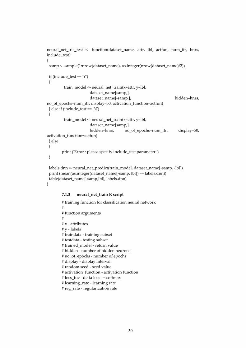
50
neural_net_iris_test <- function(dataset_name, attr, lbl, actfun, num_itr, hnrs,
include_test)
{
samp <- sample(1:nrow(dataset_name), as.integer(nrow(dataset_name)/2))
if (include_test == 'Y')
{
train_model <- neural_net_train(x=attr, y=lbl,
dataset_name[samp,],
dataset_name[-samp,], hidden=hnrs,
no_of_epochs=num_itr, display=50, activation_function=actfun)
} else if (include_test == 'N')
{
train_model <- neural_net_train(x=attr, y=lbl,
dataset_name[samp,],
hidden=hnrs, no_of_epochs=num_itr, display=50,
activation_function=actfun)
} else
{
print ('Error : please specify include_test parameter.')
}
labels.dnn <- neural_net_predict(train_model, dataset_name[-samp, -lbl])
print (mean(as.integer(dataset_name[-samp, lbl]) == labels.dnn))
table(dataset_name[-samp,lbl], labels.dnn)
}
7.1.3 neural_net_train R script
# training function for classification neural network
#
# function arguments
#
# x - attributes
# y - labels
# traindata - training subset
# testdata - testing subset
# trained_model - return value
# hidden - number of hidden neurons
# no_of_epochs - number of epochs
# display - display interval
# random.seed - seed value
# activation_function - activation function
# loss_fuc - delta loss = softmax
# learning_rate - learning rate
# reg_rate - regularization rate

51
source("neural_net_predict.R")
neural_net_train <- function(x, y, traindata=data, testdata=NULL,
model = NULL,
hidden=c(6),
no_of_epochs=2000,
loss_fuc=1e-2,
learning_rate = 1e-2,
reg_rate = 1e-3,
display = 100,
random.seed = 1,
activation_function = 'relu')
{
set.seed(random.seed)
N <- nrow(traindata)
X <- unname(data.matrix(traindata[,x]))
Y <- traindata[,y]
epoch_vector <- numeric(0)
loss_vector <- numeric(0)
accuracy_vector <- numeric(0)
if(is.factor(Y)) { Y <- as.integer(Y) }
Y_len <- length(unique(Y))
Y_set <- sort(unique(Y))
Y_index <- cbind(1:N, match(Y, Y_set))
if(is.null(model))
{
D <- ncol(X)
K <- length(unique(Y))
H <- hidden
W1 <- 0.01*matrix(rnorm(D*H), nrow=D, ncol=H)
b1 <- matrix(0, nrow=1, ncol=H)
W2 <- 0.01*matrix(rnorm(H*K), nrow=H, ncol=K)
b2 <- matrix(0, nrow=1, ncol=K)
}
else
{
D <- model$D
K <- model$K
H <- model$H
W1 <- model$W1

52
b1 <- model$b1
W2 <- model$W2
b2 <- model$b2
}
training_size <- N
loss_value <- 100000
i <- 0
while(i < no_of_epochs && loss_value > loss_fuc )
{
i <- i +1
hidden_layer <- sweep(X %*% W1 ,2, b1, '+')
if (activation_function == 'relu')
{
hidden_layer <- pmax(hidden_layer, 0)
} else if (activation_function == 'sigm')
{
hidden_layer <- 1 / 1 + (exp(hidden_layer))
} else if (activation_function == 'tanh')
{
hidden_layer <- tanh(hidden_layer)
} else
{
print('Default activation function selected!')
}
softvalue <- sweep(hidden_layer %*% W2, 2, b2, '+')
softvalue_exp <- exp(softvalue)
# Softmax probability
probs <- softvalue_exp/rowSums(softvalue_exp)
corect.logprobs <- -log(probs[Y_index])
data_loss <- sum(corect.logprobs)/training_size
reg_loss_val <- 0.5*reg_rate* (sum(W1*W1) + sum(W2*W2))
loss_value <- data_loss + reg_loss_val
if( i %% display == 0)
{
if(!is.null(testdata))
{
model <- list( D = D,
H = H,
K = K,
W1 = W1,

53
b1 = b1,
W2 = W2,
b2 = b2)
labs <- neural_net_predict(model, testdata[,-y])
accuracy <- mean(as.integer(testdata[,y]) == Y_set[labs])
cat(i, loss_value, accuracy, "\n")
epoch_vector <- c(epoch_vector, i)
loss_vector <- c(loss_vector, loss_value)
accuracy_vector <- c(accuracy_vector, accuracy)
} else
{
accuracy = 0
cat(i, loss_value, accuracy, "\n")
epoch_vector <- c(epoch_vector, i)
loss_vector <- c(loss_vector, loss_value)
accuracy_vector <- c(accuracy_vector, accuracy)
}
}
dscores <- probs
dscores[Y_index] <- dscores[Y_index] -1
dscores <- dscores / training_size
dW2 <- t(hidden_layer) %*% dscores
db2 <- colSums(dscores)
dhidden <- dscores %*% t(W2)
dhidden[hidden_layer <= 0] <- 0
dW1 <- t(X) %*% dhidden
db1 <- colSums(dhidden)
dW2 <- dW2 + reg_rate*W2
dW1 <- dW1 + reg_rate*W1
W1 <- W1 - learning_rate * dW1
b1 <- b1 - learning_rate * db1
W2 <- W2 - learning_rate * dW2
b2 <- b2 - learning_rate * db2
}
model <- list( D = D,
H = H,
K = K,
W1= W1,
b1= b1,
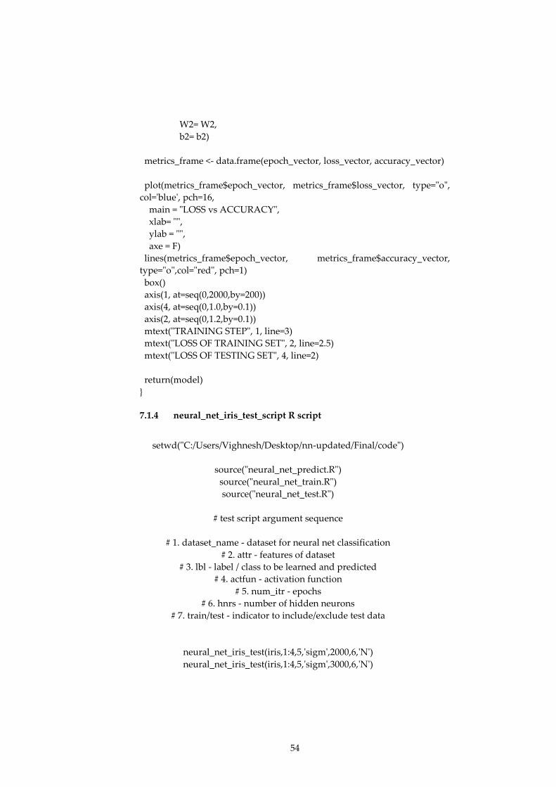
54
W2= W2,
b2= b2)
metrics_frame <- data.frame(epoch_vector, loss_vector, accuracy_vector)
plot(metrics_frame$epoch_vector, metrics_frame$loss_vector, type="o",
col='blue', pch=16,
main = "LOSS vs ACCURACY",
xlab= "",
ylab = "",
axe = F)
lines(metrics_frame$epoch_vector, metrics_frame$accuracy_vector,
type="o",col="red", pch=1)
box()
axis(1, at=seq(0,2000,by=200))
axis(4, at=seq(0,1.0,by=0.1))
axis(2, at=seq(0,1.2,by=0.1))
mtext("TRAINING STEP", 1, line=3)
mtext("LOSS OF TRAINING SET", 2, line=2.5)
mtext("LOSS OF TESTING SET", 4, line=2)
return(model)
}
7.1.4 neural_net_iris_test_script R script
setwd("C:/Users/Vighnesh/Desktop/nn-updated/Final/code")
source("neural_net_predict.R")
source("neural_net_train.R")
source("neural_net_test.R")
# test script argument sequence
# 1. dataset_name - dataset for neural net classification
# 2. attr - features of dataset
# 3. lbl - label / class to be learned and predicted
# 4. actfun - activation function
# 5. num_itr - epochs
# 6. hnrs - number of hidden neurons
# 7. train/test - indicator to include/exclude test data
neural_net_iris_test(iris,1:4,5,'sigm',2000,6,'N')
neural_net_iris_test(iris,1:4,5,'sigm',3000,6,'N')

55
neural_net_iris_test(iris,1:4,5,'sigm',2000,8,'N')
neural_net_iris_test(iris,1:4,5,'sigm',3000,8,'N')
neural_net_iris_test(iris,1:4,5,'sigm',2000,10,'N')
neural_net_iris_test(iris,1:4,5,'sigm',3000,10,'N')
neural_net_iris_test(iris,1:4,5,'sigm',2000,6,'Y')
neural_net_iris_test(iris,1:4,5,'sigm',3000,6,'Y')
neural_net_iris_test(iris,1:4,5,'sigm',2000,8,'Y')
neural_net_iris_test(iris,1:4,5,'sigm',3000,8,'Y')
neural_net_iris_test(iris,1:4,5,'sigm',2000,10,'Y')
neural_net_iris_test(iris,1:4,5,'sigm',3000,10,'Y')
neural_net_iris_test(iris,1:4,5,'tanh',2000,6,'N')
neural_net_iris_test(iris,1:4,5,'tanh',3000,6,'N')
neural_net_iris_test(iris,1:4,5,'tanh',2000,8,'N')
neural_net_iris_test(iris,1:4,5,'tanh',3000,8,'N')
neural_net_iris_test(iris,1:4,5,'tanh',2000,10,'N')
neural_net_iris_test(iris,1:4,5,'tanh',3000,10,'N')
neural_net_iris_test(iris,1:4,5,'tanh',2000,6,'Y')
neural_net_iris_test(iris,1:4,5,'tanh',3000,6,'Y')
neural_net_iris_test(iris,1:4,5,'tanh',2000,8,'Y')
neural_net_iris_test(iris,1:4,5,'tanh',3000,8,'Y')
neural_net_iris_test(iris,1:4,5,'tanh',2000,10,'Y')
neural_net_iris_test(iris,1:4,5,'tanh',3000,10,'Y')
neural_net_iris_test(iris,1:4,5,'relu',2000,6,'N')
neural_net_iris_test(iris,1:4,5,'relu',3000,6,'N')
neural_net_iris_test(iris,1:4,5,'relu',2000,8,'N')
neural_net_iris_test(iris,1:4,5,'relu',3000,8,'N')
neural_net_iris_test(iris,1:4,5,'relu',2000,10,'N')
neural_net_iris_test(iris,1:4,5,'relu',3000,10,'N')
neural_net_iris_test(iris,1:4,5,'relu',2000,6,'Y')
neural_net_iris_test(iris,1:4,5,'relu',3000,6,'Y')
neural_net_iris_test(iris,1:4,5,'relu',2000,8,'Y')
neural_net_iris_test(iris,1:4,5,'relu',3000,8,'Y')
neural_net_iris_test(iris,1:4,5,'relu',2000,10,'Y')
neural_net_iris_test(iris,1:4,5,'relu',3000,10,'Y')
7.2 Scripts for neural net using inbuilt function code
7.2.1 R script
source("neural_net_package.R")

56
neural_net_package(6, 2000)
neural_net_package(8, 2000)
neural_net_package(10, 2000)
neural_net_package(6, 3000)
neural_net_package(8, 3000)
neural_net_package(10, 3000)
7.2.1 R script
neural_net_package <- function(hn, ni) {
library(nnet)
set.seed(1)
samp <- sample(1:nrow(iris), as.integer(nrow(iris)/2))
iris_nn_model <- nnet(Species ~ .,
data = iris,
subset = samp,
size = hn, # number of hidden neurons
rang = 0.01, # initial random weights
decay = 1e-2, # weight decay
maxit = ni) # iterations
iris_nn_labels <- predict(iris_nn_model, iris[-samp,], type="class")
table(iris$Species[-samp], iris_nn_labels)
mean(iris$Species[-samp] == iris_nn_labels)
}