· web viewmodel-based production data analysis techniques are important tools for use in...

RATE-DECLINE RELATIONS FOR UNCONVENTIONAL RESERVOIRS AND DEVELOPMENT OF PARAMETRIC CORRELATIONS FOR

ESTIMATION OF RESERVOIR PROPERTIES

A Research Proposal

by

YOHANES AKLILU ASKABE

Submitted to the Office of Graduate Studies ofTexas A&M University

in partial fulfillment of the requirements for the degree of

MASTER OF SCIENCE

December 2012

Major Subject: Petroleum Engineering

Table of ContentsPage

1. Abstract......................................................................................................................................... 32. Objectives...................................................................................................................................... 43. Present Status of the Problem....................................................................................................... 44. Procedure...................................................................................................................................... 95. Analysis of Time-Rate Relations..................................................................................................

106. Development of Parametric Correlation.......................................................................................

167 Summary and Conclusion.............................................................................................................

238 Recommendation for Future Work...............................................................................................

239 Organization of the Research........................................................................................................

24Nomenclature.......................................................................................................................................

25References............................................................................................................................................

26

1. Abstract

Model-based production data analysis techniques are important tools for use in estimating the reservoir

properties of unconventional reservoirs. However, these techniques require knowledge of reservoir/well

parameters that are usually not readily available, which makes unique estimation of reservoir properties

difficult. Systematic implementation of empirical time-rate decline relations to study decline trends of

production data have been shown to provide an excellent match to the production data and provide a

reliable estimate of ultimate recovery. By using the parameters of the time-rate relation, it is possible to

formulate a parametric correlation that can provide a reliable estimate of reservoir/well properties.

Previously, Ilk et al. (2011) have shown that it is possible to correlate reservoir/well properties that are

estimated using model-based production data analysis with parameters of the power-law exponential (PLE)

time-rate relation by using limited number of wells from tight/shale gas reservoirs. From that study it was

apparent that synthetic data cases are required to obtain a more rigorous (perhaps semi-analytical)

correlation for the estimation of well/reservoir properties.

In this study, we identify relationships between reservoir properties and parameters of the time-rate

relations that are used to match time-rate data generated from a numerical simulation of a multi-fractured-

horizontal well model in a low/ultra-low permeability reservoir. Using these results, we show that the

time-rate model parameters are uniquely related to reservoir properties (specifically, we consider reservoir

permeability (k) and EUR over 30-years (EUR30-Yr)). We then formulate parametric correlations which

integrate the parameters of the time–rate relations with properties of the reservoir. We demonstrate that

when bottomhole pressure is constant (or gently changing), then the resulting correlations provide reliable

estimates of reservoir properties.

For reference, this study is performed using most "modern" time-rate relations:

● The Power Law Exponential model (PLE) (Ilk et al. 2008),

● The Duong model (Duong 2011), and

● The Logistic Growth Model (LGM) (Clark et al. 2011).

2. Introduction

In this work, we present:

● A detailed analysis of the performance of the PLE, Doung, and LGM time-rate relations in matching

time-rate data obtained from unconventional reservoirs.

● Diagnostic plots, where we show that the modern time-rate relations are effective at matching transient

and transition flow regimes observed from unconventional reservoirs. The Arps' hyperbolic model is

not used in this study as it is considered the current standard, and its strengths (excellent model for

linear and bi-linear flow) and limitations (need to be constrained (exponentially) to make realistic EUR

projections) are well-established.

( of 28)

● Use of the "continuous EUR" approach for the PLE, Doung, and LGM time-rate relations.

● Modification of the Doung and LGM time-rate relations for boundary-dominated flow behavior.

This work showcases the performance of new time-rate relations in modeling production data from

unconventional reservoirs. The modifications we have developed for the time-rate relations provide

important constraining behavior to the Duong and Logistic Growth decline models. Time-rate data match

quality is improved, EUR projections and production forecasts are improved. This work also provides a

semi-analytical basis for correlating time-rate model parameters with fundamental reservoir properties via a

numerical simulation study.

2. Objectives

The objectives of this work are:

● To compare performance of modern time-rate relations in matching production data and estimating

reserves for wells in unconventional reservoirs. We use diagnostic plots for data matching and we

apply the "continuous EUR" approach to estimate ultimate recovery in time and to compare

performance of the time-rate relations.

● To identify diagnostic relations/plots for modern time-rate models that may allow us to identify data

characteristics for better data matching/representation.

● To propose modifications of the time-rate relations to improve the quality of match and for a better

estimation of EUR, particularly for transition and boundary-dominated flow behavior.

● To develop a methodology for integration of reservoir/well properties — specifically, to demonstrate

the rigorous correlation of k and EUR30-Yr with time-rate model parameters using production data

generated from numerical simulation solutions.

3. Present Status of the Problem

Modern production data analysis techniques have become standard tools in analyzing production data from

shale gas and "liquid-rich" shale reservoirs. Analytical techniques can provide valuable information about

the formation including permeability, extent of hydraulic fracture and reserve estimates — however, in

most cases, the analysis becomes a challenge because of complex nature of the reservoir and fracture

properties. In particular, permeability is the most challenging variable to try to estimate using analytical

techniques.

In addition, the complexity of fracture networks, reservoir heterogeneity, stress dependence of permeability

and porosity and changes in conductivity can make unique estimation of reservoir parameters a difficult, if

not non-unique task. In-addition, operational complications such as liquid loading can result in erratic

production rate and surface pressure data, which are not altogether representative of the conditions at the

formation. As noted, these circumstances can (and do) lead to non-unique, if not erroneous solutions.

( of 28)

On the other hand, empirical time-rate decline relations are used regularly because these require only time-

rate data as inputs. However, since most time-rate decline models have an empirical basis (or highly

idealized conditions of application), these relations do not convey fundamental characteristics of the

reservoir. Statistical analyses of the power-law exponential (or PLE) time-rate model parameters have been

shown to provide a somewhat unique insight in to the performance of the reservoir, and it is logical to

assume that other models may do so as well. Specifically, factors that may affect well performance such as

the effectiveness of well completions and characteristics of the reservoir for example reservoir boundary

conditions can be identified/isolated by statistically studying the time-rate model parameters (Arps 1945;

Clark et al. 2011; Duong 2011; Fetkovich et al. 1996).

Arps (1945) rate decline models have been used widely to forecast production and estimate reserves from

conventional oil and gas wells. However, it has been shown that Arps hyperbolic model overestimates

reserves by more than 100 percent when used to match wells producing from unconventional low/ultra-low

permeability reservoirs (Rushing et al. 2007). In the past decade several new time-rate relations have been

presented with improvements to analyze time-rate data from unconventional reservoirs. Ilk et al. (2008)

have presented a power law exponential model (PLE) based on the "loss-ratio" and the "loss-ratio

derivative" definitions (Johnson and Bollens 1927). The PLE model provides a superior match quality to

the transient, transitional and boundary dominated flow-regimes observed from wells producing from

unconventional resources.

A stretched exponential model (SEPD) was independently presented by Valko (2009) after studying flow

characteristics of over 7000 wells in the Barnet Shale. The SEPD model is the same as the base form of the

PLE model (without the terminal decline term); the SEPD models the long transient and transitional flow

regimes observed in production data from unconventional gas reservoirs — however; it lacks the boundary-

dominated flow term present in the PLE model.

Duong (2011) presented a time-rate decline model for fracture linear flows producing at a constant flowing

bottomhole pressure. Duong derived his relation based on the observation of a straight line behavior in

q/Gp vs. time on a log-log plot. The Duong model can match transient characteristics that are dominant in

low/ultra-low permeability fractured reservoirs, but this model is incapable of representing boundary-

dominated flow performance. The slope and intercept of the straight-line portion of the log(q/Gp) vs.

log(time) data show narrow ranges for reservoirs with similar reservoir rock types and fracture

characteristics.

Clark et al. (2011) adapted the hyperbolic form of the "logistic growth model" for reserve estimation of oil

and gas reservoirs. Blumberg (1968) suggested this hyperbolic form to characterize regenerative growth in

biological systems. The hyperbolic nature of the LGM provides a good match for transient and transition

flow regimes of wells from unconventional reservoirs, but this relation does not model boundary-

dominated flow well.

( of 28)

There have been attempts in the past to link fundamental reservoir properties with time-rate model

parameters. Fetkovich (1980) has shown that time-rate models which are analogous to Arps empirical

models can be derived analytically from solutions of oil and gas wells producing from a reservoir at a

constant flowing bottomhole pressure condition. This means that Arps time-rate model parameters are

more than simple empirical parameters. Instead these parameters are characteristics (or proxies of

characteristics) of the reservoir and can convey fundamental reservoir properties. Another approach to link

empirical time-rate model parameters with reservoir properties was proposed by Ilk et al. (2011). In their

study, the authors demonstrated that it is possible to correlate time-rate model parameters (PLE) with

reservoir parameters (k and kxf) by using small number of wells producing from tight/shale gas reservoirs.

From that study it was concluded that more data is required for conclusively unique results.

The main objective of this study is to investigate performance of modern time-rate models in matching

time-rate data from unconventional reservoirs. Our strategy in this investigation is:

● Prepare diagnostic relations/analyses using each rate decline models.

● Compare the performance of each models for transient, transition and boundary dominated flow.

● Use the "continuous EUR" approach to estimate reserves for both synthetic and a field data.

● Compare the relative accuracy of reserve estimates made with the modern time-rate models.

● Propose modified time-rate relations that better capture flow regimes for unconventional reservoirs.

Also, we present more rigorous basis for the work presented by Ilk et al. (2011) using time-rate data

generated from a numerical simulator to demonstrate a methodology for integrating fundamental reservoir

properties (k and EUR) with time-rate model parameters. We show that the derived parametric correlations

provide a reliable estimate of the reservoir properties for wells producing with similar production

constraints.

As background regarding our diagnostic approach, we begin with the work of Ilk et al. (2008) where they

demonstrated the application of the "loss-ratio" and the "loss-ratio" derivative relations as diagnostic tools

for matching time-rate data. The definitions of the D(t) function (i.e., the reciprocal of the "loss ratio") and

b(t) function (i.e., the "loss-ratio" derivative) are given by Eqs. 1 and 2.

D( t )=− 1qg

dqg

dt ......................................................................................................................................(1)

b ( t )= ddt [ 1

D( t ) ] .......................................................................................................................................(2)

Multiplying the D(t) function by the production time (t) provides another diagnostic relation that we can

also use to match the rate time data. This relation is known as the "beta function" (β(t)) and is given by:

β ( t )=tD ( t )..............................................................................................................................................(3)

( of 28)

( of 28)

The time–rate empirical models considered in this research include:

● The Power Law Exponential model (PLE) (Ilk et al. 2008),

● The Duong model (Duong 2011), and

● The Logistic Growth Model (LGM) (Clark et al. 2011).

Following we will provide a short description of the time–rate models.

Power Law Exponential Model

The power–law exponential model was derived by observing the "loss-ratio" behavior of wells producing

from low/ultra–low permeability reservoirs producing through fracture stimulation. Ilk et al. (2008)

demonstrated that by describing the "loss–ratio" of the data using a power–law function, it is possible to

match the dominant transient and transition flow regimes observed from unconventional reservoirs. In

addition, boundary dominated flow regimes are represented by adding a decline term (D∞) to the power law

relation. The PLE model "loss-ratio" relation is given by Eq. 4.

D( t )=D∞+ Di ntn−1................................................................................................................................(4)

During late-time flow periods, the power-law term becomes less significant and D(t) approaches a constant

term (D∞) similar to the case in Arps exponential decline model. Furthermore, the authors observed that the

derivative of the "loss-ratio" is not constant as was the case in Arps' rate decline relations ( i.e., exponential,

hyperbolic and harmonic equations), but instead it is a function of time. The "loss-ratio" derivative ( b-

parameter) is given by:

b ( t )=−Di (n−1 )ntn

( D∞ t+Di ntn )2............................................................................................................................(5)

And the PLE "beta" relation is given by:

β ( t )=D∞+ Di nt n....................................................................................................................................(6)

And the power-law exponential rate relation is given by Eq. 7.

q=qgi exp[−D∞ t−Di tn ] ..........................................................................................................................(7)

As mentioned earlier a diagnostic plot of D(t) ,b(t) and β(t) vs. time will help diagnose the time-rate data

matching process

Duong’s Model

Duong (2011) presented a new empirical rate decline model based on the long-term linear or bilinear flow

regimes observed in hydraulically fractured ultra-low permeability reservoirs. On a log-log plot of rate vs.

( of 28)

time, the early time data shows half slope for linear flow and quarter slope for bilinear flow regimes. A

log-log plot of rate over cumulative production vs. time will result in a straight line for wells producing

from unconventional reservoirs. This straight line behavior is described by a power-law relation given by

Eq. 8.

qGp

=at−m

.................................................................................................................................................(8)

Where:

a = straight line intercept on log-log plot of q/Gp vs. time

m = negative slope of straight line on log-log plot of q/Gp vs. time.

The slope and intercept parameters of Duong model show narrow ranges for wells producing from similar

rock-types and similar fracture stimulation practices and operational conditions (Duong 2011). The

parameters can be directly estimated from q/Gp vs. time diagnostic plot.

The Duong rate and cumulative relations are given by Eq. 9 and Eq. 10 respectively.

qq1

=t−m exp [ a1−m

( t1−m−1)]..................................................................................................................(9)

Gp=q1

aexp [ a

1−m( t1−m−1)] ................................................................................................................(10)

In addition to q/Gp vs. time log-log diagnostic plot, we will use the "loss-ratio" and the "loss-ratio"

derivative definitions to estimate the model parameters and guide the data matching process. The b, D and

β-parameters of Duong model are given by Eqs. 11, 12 and 13 respectively.

D( t )=mt−1−at−m..................................................................................................................................(11)

b ( t )=mtm( tm−at )(at−mtm )2

...............................................................................................................................(12)

β ( t )=m−at−m......................................................................................................................................(13)

We can also estimate the m parameter independently using the following diagnostic relation:

tGp

qddt [ q

Gp ]=m..................................................................................................................................(14)

Logistic Growth Model

( of 28)

Yet another model, the Logistic Growth Model (LGM) is adapted to model time-rate data from oil/gas

reservoirs. The LGM is originally developed to model growth trends of various populations in nature. A

form of the logistic growth model has been used to model growth of yeast and to study market penetration

of new products and technologies (Martinez et al. 2008). Tsoularis and Wallace (2002) have derived a

general form of the logistic growth model. They have also presented a summary of various logistic growth

models for various applications.

Clark (2011) adapted the hyperbolic form of the logistic growth model to match time-rate data of oil/gas

reservoirs. The hyperbolic form was suggested by (Blumberg 1968) to study regenerative growth in nature.

Eq. 15 shows the hyperbolic form of the logistic growth model.

N ( t )= K ( t+b )n

a+( t+b)n.................................................................................................................................(15)

Clark et al. (2011) applied this model to several oil and gas wells and noted that the b parameter

consistently becomes zero. After eliminating the parameter b and rearranging, the cumulative form of the

hyperbolic logistic growth model is given by:

Q( t )= Kt n

a+ tn.........................................................................................................................................(16)

The time-rate form is given by Eq. 17.

q ( t )= a K n tn−1

( a+t n )2.....................................................................................................................................(17)

Similarly the "loss-ratio" (b) and the "loss-ratio" derivatives (D) of the logistic growth model will be used

to perform diagnostic match of time-rate data. Logistic growth model b, D and β parameters are given by

Eqs. 18 , 19 and 20 respectively.

D( t )= a−a n+(1+ n) t n

t( a+t n ) ......................................................................................................................(18)

b ( t )=−a2 ( n−1 )−2 a( n2−1 )t n+( n+1) t2n

( a−a n+( n+1) tn )2.......................................................................................(19)

β ( t )= a−a n+(1+ n) t n

( a+t n ) ......................................................................................................................(20)

And the q/Gp formulation of LGM is given by:

qGp

=t ( a+tn

a n )........................................................................................................................................(21)

( of 28)

If the initial gas in place is known, we can rewrite the rate relation to find a diagnostic relation that will

allow a diagnostic plot estimation of the remaining model parameters (Clark et al. 2011).

KQg ( t )

−1=a t−n

.......................................................................................................................................(22)

4. Procedure

As an introduction to the time-rate models discussed here, prior to developing the parametric correlations,

we will investigate the performance of the rate decline models in matching time-rate data from

unconventional reservoirs. We will perform data driven model matching using the "loss-ratio", the "loss-

ratio" derivative relations as well as other diagnostic relations. We will also study performance of the time-

rate relations using the "continuous EUR" approach. Then we will modify the time-rate models to better

estimate EUR and accurately forecast production.

We will demonstrate development of a parametric correlation using a set of production data generated from

a simulated multi-fractured horizontal well model. First, we will study a cross-plot of the rate-decline

model parameters and reservoir properties, particularly, permeability (k) and EUR30-Yr. This will allow us

identify a parametric function that best correlates the rate-decline model parameters with the reservoir

properties. Once we know the relationship between the model parameters and the reservoirs properties, we

will develop the correlating function for estimation of reservoir properties.

5. Analysis of Modern Time-Rate Relations

Time-rate data generated from a set of numerical models of a multi-fractured horizontal well is matched

using the empirical rate decline relations discussed above. A set of numerical models, with permeability

values ranging from 0.25µD-5µD, are used to generate the production data. Other reservoir, fluid and well

parameters are kept constant.

Fig. 1 shows a schematic of the reservoir model we are considering in this study. It depicts a horizontal

well that is producing from low/ultra-low permeability reservoir producing through multistage fracture

stimulation.

Transverse fractures Horizontal well

( of 28)

Figure 1 — A schematic of a numerical simulation model. (Horizontal well with multiple transverse

fractures)

Table 1 shows a summary of the model input parameters.

Table 1 — Reservoir and fluid properties for simulated horizontal shale gas well model with multiple transverse fractures.

Reservoir Properties:Net pay thickness, h = 130 ftFormation permeability, k = 0.25µD-5µDWellbore Radius, rw = 0.35 ftFormation compressibility, cf = 3 x 10-6 psi-1

Porosity, = 0.09 (fraction)Initial reservoir pressure, pi = 5000 psiGas saturation, sg = 1.0 fractionSkin factor, s = 0.01 (dimensionless)Reservoir temperature, Tr = 212 °F

Fluid properties:Gas specific gravity, γg = 0.6 (air = 1)

Hydraulically fractured well model parameters:Fracture half-length, xf = 164.0 ftNumber of fractures = 15Horizontal well length = 4921.3 ft

Production parameters:Flowing pressure, pwf = 500 psiaProduction time, t = 10,958 days (30 years)

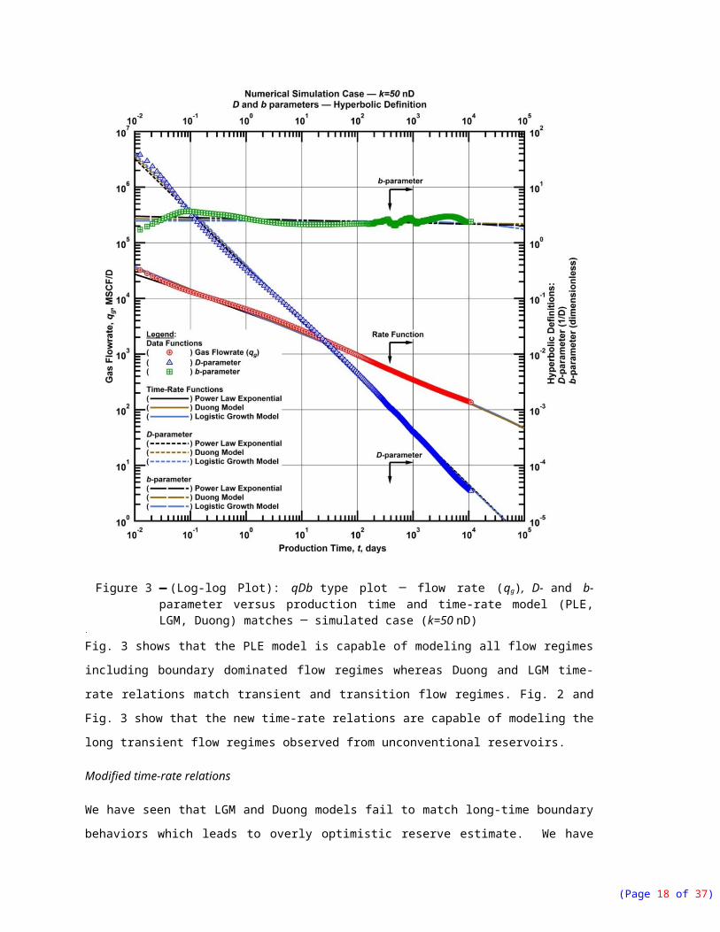
Fig. 2 and Fig. 3 shows a "qDb" type diagnostic plot of a time-rated data match using the PLE, LGM and

Duong time-rate relations. The diagnostic relations will provide a systematic and data driven estimation of

the model parameters. When there is no restriction on the degree of freedom, it is possible to obtain a wide

range of parameters that result in a model fit.

( of 28)

Figure 2 — (Log-log Plot): qDb type plot ─ flow rate (qg), D- and b- parameter versus production time and time-rate model (PLE, LGM, Duong) matches ─ simulated case (k=800 nD)

( of 28)

Figure 3 — (Log-log Plot): qDb type plot ─ flow rate (qg), D- and b- parameter versus production time and time-rate model (PLE, LGM, Duong) matches ─ simulated case (k=50 nD)

.

Fig. 3 shows that the PLE model is capable of modeling all flow regimes including boundary dominated

flow regimes whereas Duong and LGM time-rate relations match transient and transition flow regimes. Fig.

2 and Fig. 3 show that the new time-rate relations are capable of modeling the long transient flow regimes

observed from unconventional reservoirs.

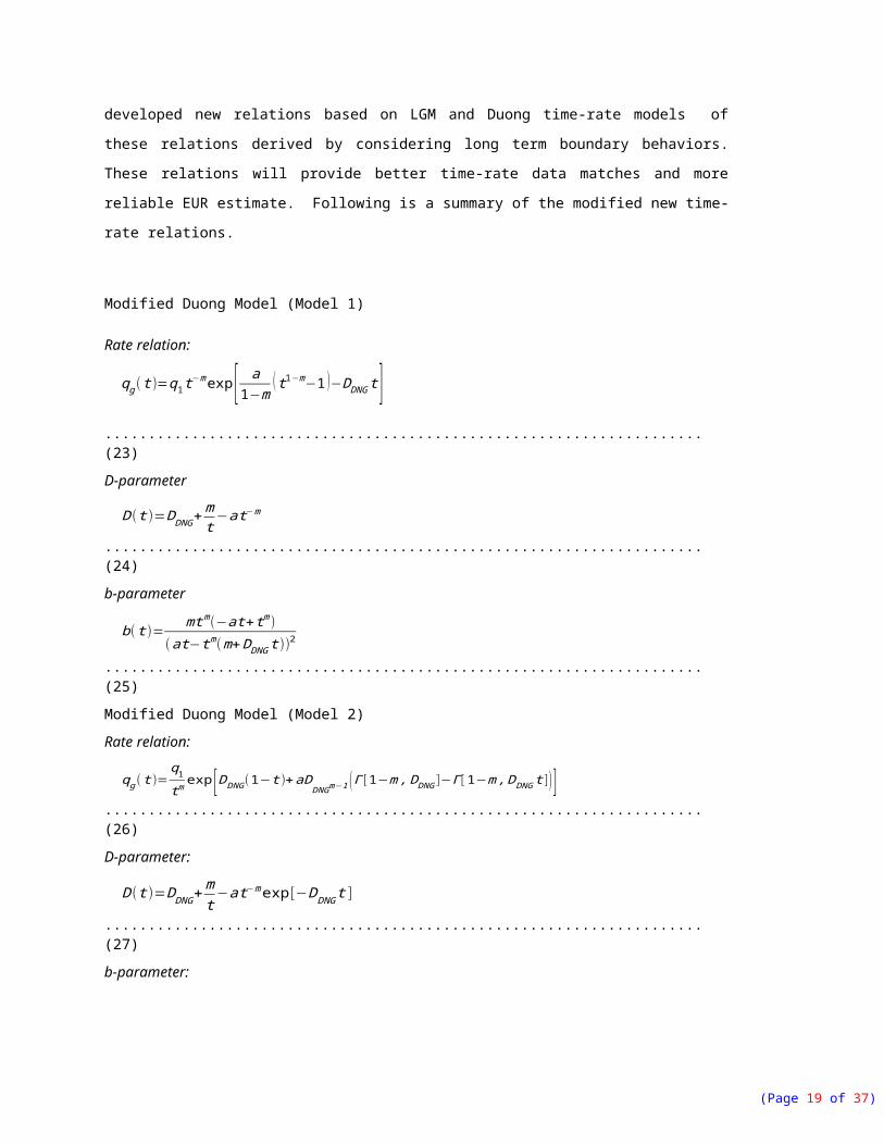
Modified time-rate relations

We have seen that LGM and Duong models fail to match long-time boundary behaviors which leads to

overly optimistic reserve estimate. We have developed new relations based on LGM and Duong time-rate

models of these relations derived by considering long term boundary behaviors. These relations will

provide better time-rate data matches and more reliable EUR estimate. Following is a summary of the

modified new time-rate relations.

( of 28)

Modified Duong Model (Model 1)

Rate relation:

qg ( t )=q1 t−mexp [ a1−m

( t1−m−1 )−DDNG t ].......................................................................................(23)

D-parameter

D( t )=DDNG+ mt−at−m

.........................................................................................................................(24)

b-parameter

b ( t )= mtm(−at+tm)(at−tm(m+DDNG t ))2

..............................................................................................................(25)

Modified Duong Model (Model 2)

Rate relation:

qg ( t )=q1

t m exp [DDNG(1−t )+aDDNGm−1 (Γ [1−m, DDNG ]−Γ [ 1−m ,DDNG t ])] .......................................(26)

D-parameter:

D( t )=DDNG+ mt−at−m exp[−DDNG t ]

...............................................................................................(27)

b-parameter:

b ( t )=exp[ DLGM t ] tm (exp[ DLGM t ]mtm−at (m+DLGM t ))

(at−exp[ DLGM t ] tm(m+DLGM t ))2 .........................................................................(28)

Modified LGM (Model 3)

Rate relation:

qg ( t )=aKnt (n−1)

(a+ tn )2 exp[−DLGM t ]..........................................................................................................(29)

D-parameter:

D( t )=a (1−n+DLGM t )+tn(1+n+DLGM t )

t (a+tn ) ....................................................................................(30)

b-parameter

b ( t )= −a2(n−1)−2a (n2−1) tn+(n+1) t2 n

(a(1−n+DLGM t )+tn(1+n+DLGM t ))2................................................................................(31)

Modified LGM (Model 4)

Rate relation:

qg ( t )=Ktn−1 a exp[ DLGM t ](n+DLGM t )

(a+(1+R )exp [DLGM t ] tn)2 ...............................................................................................(32)

Cumulative production:

( of 28)

Qg( t )=Kt n exp[−DLGM t ]

a+(1+R)exp [ DLGM t ] tn.......................................................................................................(33)

The modified relations are capable of matching long-term time production data obtained from

unconventional reservoirs. These new models constrain the EUR estimates and provide more reliable

production forecasts. Figs. 4 and 5 show the improved match quality of the modified LGM and Duong

time-rate models.

Figure 4 — (Log-log Plot): qDb type plot ─ flow rate (qg), D- and b- parameter versus production time and time-rate model (Duong Model, Modified Duong Model (Model 3), Modified Duong Model (Model 4)) matches ─ simulated case (k=8 µD)

( of 28)

Figure 5 — (Log-log Plot): qDb type plot ─ flow rate (qg), D- and b- parameter versus production time and time-rate model (LGM, Modified LGM (Model 3), Modified LGM (Model 4)) matches ─ simulated case (k=8 µD)

We have done model matches of 14 synthetic well models generated using varying permeability values. In

addition, we will investigate the performance of the empirical models in matching production data from

unconventional reservoirs. Also, we will estimate reserves using the “continuous EUR” approach and

compare the performance of the time-rate relations.

6. Development of parametric correlations

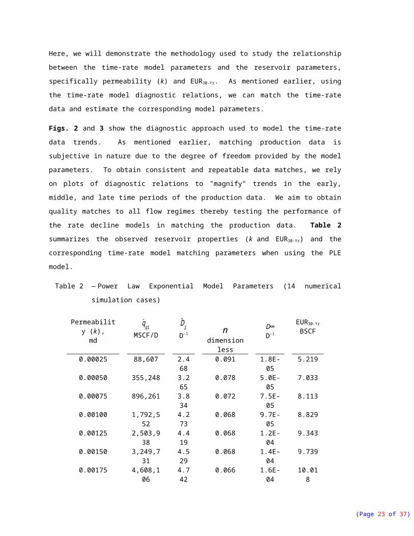
Here, we will demonstrate the methodology used to study the relationship between the time-rate model

parameters and the reservoir parameters, specifically permeability (k) and EUR30-Yr. As mentioned earlier,

using the time-rate model diagnostic relations, we can match the time-rate data and estimate the

corresponding model parameters.

( of 28)

Figs. 2 and 3 show the diagnostic approach used to model the time-rate data trends. As mentioned earlier,

matching production data is subjective in nature due to the degree of freedom provided by the model

parameters. To obtain consistent and repeatable data matches, we rely on plots of diagnostic relations to

"magnify" trends in the early, middle, and late time periods of the production data. We aim to obtain

quality matches to all flow regimes thereby testing the performance of the rate decline models in matching

the production data. Table 2 summarizes the observed reservoir properties (k and EUR30-Yr) and the

corresponding time-rate model matching parameters when using the PLE model.

Table 2 — Power Law Exponential Model Parameters (14 numerical simulation cases)

Permeability (k),md

qgiMSCF/D

DiD-1

ndimensionless

D∞D-1

EUR30-Yr

BSCF

0.00025 88,607 2.468

0.091 1.8E-05 5.219

0.00050 355,248 3.265

0.078 5.0E-05 7.033

0.00075 896,261 3.834

0.072 7.5E-05 8.113

0.00100 1,792,552 4.273

0.068 9.7E-05 8.829

0.00125 2,503,938 4.419

0.068 1.2E-04 9.343

0.00150 3,249,731 4.529

0.068 1.4E-04 9.739

0.00175 4,608,106 4.742

0.066 1.6E-04 10.018

0.00200 5,937,051 4.875

0.066 1.7E-04 10.240

0.00250 9,396,501 5.139

0.065 2.0E-04 10.585

0.00300 13,723,998

5.362

0.064 2.4E-04 10.799

0.00350 18,706,208

5.543

0.064 2.7E-04 10.967

0.00400 23,653,940

5.666

0.064 3.0E-04 11.082

0.00450 30,171,081

5.816

0.063 3.3E-04 11.170

0.00500 38,246,539

5.973

0.062 3.6E-04 11.245

Next, to provide a basis for developing the parametric correlation, we need to demonstrate how the rate

decline model parameters are related to the reservoir parameters. We will construct a series of cross-plots

to determine how the rate decline model parameters are varying with the reservoir/well properties. Figs. 4 -

6 show permeability plotted against the PLE model parameters and Figs. 7-9 Show EUR30-Yr plotted against

the PLE model parameters. The plots also show results of a regression analysis along with the best fit trend

line function. From the cross-plots it is evident that the PLE model parameters show behaviors that could

( of 28)

be described by parametric functions. We will apply similar analysis using Duong and LGM time-rate

relations.

Figure 6 — (Cartesian Plot): Cross plot of permeability and PLE n-Parameter—simulated case.

( of 28)

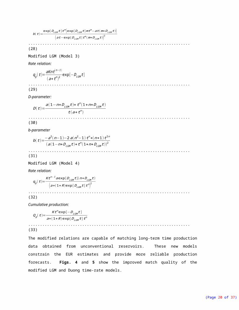
Figure 7 — (Cartesian Plot): Cross plot of permeability and PLE Di -parameter—simulated case.

( of 28)

Figure 8 — (Cartesian Plot): Cross plot of permeability and PLE qgi -parameter —simulated case.

Figure 9 — (Cartesian Plot): Cross plot of EUR30-Yr and PLE n-parameter —simulated case.

Figure 10 — (Cartesian Plot): Cross plot of EUR30-Yr and PLE Di -parameter—simulated case.

( of 28)

Figure 11 — (Cartesian Plot): Cross plot of EUR30-Yr and PLE-qgi -parameter—simulated case.

The cross-plots describe the relationship between the model parameters and the reservoir properties. The

parametric functions we choose to correlate the individual model parameters with the reservoir properties

should result in a best-fit to the data. The coefficient of determination ("R-squared") value indicates the

accuracy of the selected parametric function in describing the correlation.

The final task is to formulate a function with the rate decline model parameters as variables to estimate the

reservoir properties. Since the rate decline model parameters represent characteristic of the production data

and of the diagnostic relations, it is fair to assume a form of the function that contains the parametric

functions we defined for each model parameter earlier (Figs. 6-11). For example, from Figs. 6-8 we can

see that permeability (k) is related to PLE model parameters, n,Di , and qgi via a power function. From

this we can suggest the following integrating parametric function.

k=a01na02 D

ia03

^qgi

a04 ......................................................................................................................(34)

Where:

a01 = model parameter, md-D2/MSCFa02 = model parameter, n-parameter exponent, dimensionless

a03 = model parameter Di -parameter exponent, dimensionless

a04 = model parameter qgi -parameter exponent, dimensionless

( of 28)

Similarly, EUR can be estimated by the parametric correlation:

EUR=a05 ln ( a06 D i)exp(a07n ) ............................................................................................................(35)

Where:

a05 = model parameter, BSCFa06 = model parameter, Daysa07 = model parameter, dimensionless

Once we establish a form of the parametric equation, we will perform regression analysis to determine the

coefficients and exponents of the parametric correlations. It should be noted that it may not be necessary to

have all time-rate model parameters present in the correlation. Coefficients and exponents that gave best

estimate of the reservoir/well properties are selected. In some cases the exponents or coefficients can

become zero. In such cases, the parameter is eliminated from the final equation. It can be seen that the

qgimodel parameter does not appear in the EUR parametric equation (Eq. 35).

A correlation plot of permeability (k) and EUR30-Yr is shown on Figs. 12 and 1,3 respectively. The figures

show that it is possible to formulate a parametric correlation that estimates reservoir properties from time-

rate relation parameters when reservoir properties such as flowing bottomhole pressure (pwf) and

completion parameters (e.g., number of fracture stages) remain constant. The figures show that the

developed correlations were able to provide a reliable estimate of the reservoir properties.

( of 28)

Figure 12 — (Log-log Plot): Comparison of permeability (k) calculated using permeability correlation versus simulated case model permeability.

Figure 13 — (Log-log Plot): Comparison of EUR30-Yr calculated using EUR correlation versus simulated case model EUR30-Yr.

We require that the time-rate relations provide reliable reserve estimates before we attempt to develop the

parametric correlation. Reliable reserve estimate and quality time-rate data match indicates that the model

parameters are related to fundamental reservoir characteristics.

7. Summary and Conclusion

Summary:

In this work we have executed a performance analysis of modern rate decline models (PLE, LGM, and

Duong) using diagnostic relations and diagnostic plots, in matching the production data and estimating

reserves of unconventional reservoirs. We have shown that new time-rate relations are capable of

modeling the dominant transient and transition flow regimes observed from production data analysis of

hydraulically fractured wells in low/ultra-low permeability reservoirs. We have shown that PLE model is

capable of modeling boundary dominated flow regimes whereas LGM and Duong models lack boundary

characteristics. The "continuous EUR" approach is used to study performance of the time-rate models in

estimating ultimate recovery. Finally, we have proposed new time rate-relations to improve the reserve

estimates and production forecasts of these (Duong, LGM) models. The proposed time-rate relations

include boundary conditions to model observed long-time boundary-dominated flow regimes and to

constrain reserve estimates.

( of 28)

In addition, we have developed a methodology to formulate a parametric correlation to integrate reservoir

properties with rate decline model parameters by analyzing time-rate data generated from a reservoir

simulation of a multi-fractured horizontal well in low/ultra-low permeability reservoir. The developed

correlations will allow estimation of reservoir properties using parameters of the time-rate models. When

unique estimates of reservoir parameters are missing to allow a complete model based production data

analysis, these correlations will permit fast estimation of fundamental reservoir properties (permeability (k)

and EUR) by using time-rate data which is readily available. This theoretical consideration shows that

when bottomhole flowing pressure is constant, it is possible to correlate empirical time-rate model

parameters with reservoir properties (k and EUR).

Conclusions:

● We have compared performance of PLE, LGM and Duong time-rate relations when used to model

production data from unconventional reservoirs. We have demonstrated various diagnostic relations

and a diagnostic plot method of estimating the model parameters. We have also used the "continuous

EUR" approach to compare degrees of convergence of reserve estimates from these new time-rate

relations.

● We have modified the LGM and Duong time-rate models to obtain relations that can better model

transient, transition and boundary-dominated flow regimes.

● Theoretical consideration for integrating time-rate model parameters with reservoir model parameters

is presented using time-rate data generated from a numerical simulator. The parametric correlations

can provide fast estimates of fundamental reservoir properties when unique estimation is not possible

from model-based production data analysis.

8. Recommendations for Future Work

We have presented a theoretical validation for estimation of reservoir properties using parametric

correlations. Future study will focus on developing the method using a high quality field data.

( of 28)

9. Organization of the Research

Following is outline of the proposed research:

● Chapter I — Introduction

■ Statement of problem■ Objectives■ Organization

● Chapter II — Literature Review

■ Empirical, Semi-Analytical, and Empirical Production Data Analysis ■ Integrated Production Data Analysis■ Data Diagnosis■ Reservoir properties from time-rate data analysis

● Chapter III — Analysis of Modern Time-Rate Relations

■ Modern Time-Rate Relations■ Analysis of Time-Rate Data■ Reserve Estimation-"Continuous EUR"■ Modified time-rate relation

● Chapter IV — Development of Parametric Correlation

■ Methodology■ Analysis of Model Parameters■ Parametric Correlation

● Chapter V — Summary and conclusion

■ Summary■ Conclusion■ Recommendation for future work

● Nomenclature

● References

( of 28)

Nomenclaturea = Duong model intercept defined by Eq. 7, 1/Db = "Loss-ratio" derivative, dimensionlessa = LGM time-rate equation model parameter (Eq. 13), Daysa01 = Model parameter for empirical correlation, md-D2/MSCFa02 = Model parameter for empirical correlation, dimensionlessa03 = Model parameter for empirical correlation, dimensionlessa04 = Model parameter for empirical correlation, dimensionlessa05 = Model parameter for empirical correlation, BSCFa06 = Model parameter for empirical correlation, Daysa07 = Model parameter for empirical correlation, dimensionless

b = LGM time-rate equation model parameter, DD = "Loss-ratio", 1/DD∞ = Power-law exponential decline relation at infinite time, 1/DDDNG = Modified Duong model decline parameter, 1/D

Di = Power-law exponential decline relation, 1/D DLGM = Modified Duong model decline parameter, 1/DEUR = Estimated ultimate recovery, MSCFEUR30-Yr = Estimated ultimate recovery after 30 years, MSCFk = Model permeability, mdK = LGM model parameter (Carrying capacity), MSCFm = Duong model Slope defined by Eq. 7, dimensionlessn = Power-law exponential relation time exponent, dimensionlessn = LGM time-rate relation model parameter (Eq. 13), dimensionlessq1 = Rate at day 1, MSCF/Dqgi = Power-law exponential relation rate intercept, MSCF/Dt = Production time, daysxf = Fracture half-length, ft

( of 28)

References

Arps, J.J. 1945. Analysis of Decline Curves. 945228-G

Blumberg, A.A. 1968. Logistic Growth Rate Functions. Journal of Theoretical Biology 21 (1): 42-44.

Clark, A.J. 2011. Decline Curve Analysis in Unconventional Resource Plays Using Logistic Growth Models. M.S Thesis, . The University of Texas at Austin.

Clark, A.J., Lake, L.W., and Patzek, T.W. 2011. Production Forecasting with Logistic Growth Models. Paper presented at the SPE Annual Technical Conference and Exhibition, Denver, Colorado, USA. Society of Petroleum Engineers SPE-144790-MS.

Duong, A.N. 2011. Rate-Decline Analysis for Fracture-Dominated Shale Reservoirs. SPE Reservoir Evaluation & Engineering (06). 137748-PA

Fetkovich, M.J. 1980. Decline Curve Analysis Using Type Curves. SPE Journal of Petroleum Technology 32 (6). 4629

Fetkovich, M.J., Fetkovich, E.J., and Fetkovich, M.D. 1996. Useful Concepts for Decline Curve Forecasting, Reserve Estimation, and Analysis. SPE Reservoir Engineering 11 (1): 13-22. 28628-PA

Ilk, D., Rushing, J.A., and Blasingame, T.A. 2011. Integration of Production Analysis and Rate-Time Analysis Via Parametric Correlations -- Theoretical Considerations and Practical Applications. Paper presented at the SPE Hydraulic Fracturing Technology Conference, The Woodlands, Texas, USA. 140556.

Ilk, D., Rushing, J.A., Perego, A.D. et al. 2008. Exponential Vs. Hyperbolic Decline in Tight Gas Sands: Understanding the Origin and Implications for Reserve Estimates Using Arps' Decline Curves. Paper presented at the SPE Annual Technical Conference and Exhibition, Denver, Colorado, USA. Society of Petroleum Engineers.

Jay Alan, R., Albert Duane, P., Richard, S. et al. 2007. Estimating Reserves in Tight Gas Sands at Hp/Ht Reservoir Conditions: Use and Misuse of an Arps Decline Curve Methodology. Paper presented at the SPE Annual Technical Conference and Exhibition, Anaheim, California, U.S.A. 109625.

Johnson, R.H. and Bollens, A.L. 1927. The Loss Ratio Method of Extrapolating Oil Well Decline Curves.

Martinez, A.S., González, R.S., and Terçariol, C.A.S. 2008. Continuous Growth Models in Terms of Generalized Logarithm and Exponential Functions. Physica A: Statistical Mechanics and its Applications 387 (23): 5679-5687.

Tsoularis, A. and Wallace, J. 2002. Analysis of Logistic Growth Models. Mathematical Biosciences 179 (1): 21-55. (submitted 2002/8//)

Valko, P.P. 2009. Assigning Value to Stimulation in the Barnett Shale: A Simultaneous Analysis of 7000 Plus Production Histories and Well Completion Records. Paper presented at the SPE Hydraulic Fracturing Technology Conference, The Woodlands, Texas. Society of Petroleum Engineers SPE-119369-MS.

( of 28)

· web viewmodel-based production data analysis techniques are important tools for use in...

Documents