VideoEdge: Processing Camera Streams using Hierarchical Clusters

Chien-Chun HungMicrosoft Research / University of Southern California

Ganesh AnanthanarayananMicrosoft Research

Peter BodikMicrosoft Research

Leana GolubchikUniversity of Southern California

Minlan YuHarvard University

Paramvir BahlMicrosoft Research

Matthai PhiliposeMicrosoft Research

ABSTRACTOrganizations deploy a hierarchy of clusters – cameras,

private clusters, public clouds – for analyzing live videofeeds from their cameras. Video analytics queries havemany implementation options which impact their resourcedemands and accuracy of outputs. Our objective is to selectthe “query plan” – implementations (and their knobs) – andplace it across the hierarchy of clusters, and merge commoncomponents across queries to maximize the average queryaccuracy. This is a challenging task, because we have toconsider multi-resource (network and compute) demandsand constraints in the hierarchical cluster and search in anexponentially large search space for plans, placements, andmerging. We propose VideoEdge, a system that introducesdominant demand to identify the best tradeoff between mul-tiple resources and accuracy, and narrows the search spaceby identifying a “Pareto band” of promising configurations.VideoEdge also balances the resource benefits and accuracypenalty of merging queries. Deployment results show thatVideoEdge improves accuracy by 25.4× and 5.4× comparedto fair allocation of resources and a recent solution forvideo query planning (VideoStorm [69]), respectively, andis within 6% of optimum.

I. INTRODUCTION

Major cities like New York and Beijing are deployingthousands of cameras. Analyzing live video streams fromthese cameras is of considerable importance to organizations.Traffic departments analyze video streams from camerasat intersections for traffic control, and police departmentsanalyze city-wide cameras for surveillance.

Organizations commonly deploy a hierarchy of clustersto analyze their video streams. Every organization, e.g., atraffic department, runs its private cluster to pull in thevideo feeds from its cameras (with dedicated bandwidths).The private cluster contains compute for analytics while alsotapping into public clouds (like Amazon EC2) for overflowcompute. The uplink bandwidth between the private clusterand the public cloud, however, is not sufficient to streamall the camera feeds to the cloud for analytics, and theavailable network capacity could vary [1]. Some newercameras also have compute capacity on them. Major video

analytics providers like Genetec [8] and Avigilon [4], marketstudies [15], as well as cloud providers like Amazon andMicrosoft [13] indicate that the hierarchical architecture –camera, private cluster, cloud – is indeed common and theonly feasible approach for large scale analytics of videostreams. The suitability of a hierarchical architecture is alsoreflected in our partnership with the City of Bellevue, WA,and City of Washington, DC that are deploying our trafficvideo analytics solution [42].

Video analytics queries are a pipeline of computer visioncomponents. For example, the object tracking query consistsof a “decoder” component, followed by an object “detector”,and an “associator” component. Each component has manyimplementation choices that provide the same abstraction.For example, object detectors take a frame and output a listof detected objects. Detectors can use background subtrac-tion to identify moving objects against a static backgroundor a deep neural network (DNN) to detect objects based onvisual features. Components and their implementations areanalogical to logical and physical operators in SQL queries.

Different implementations have different resource de-mands and produce outputs of varying accuracies. To detectobjects, background subtraction requires fewer resourcesthan a DNN but is also less accurate because it missesstationary objects. Core vision components have tens ofdifferent implementations but no single one that is cheapestand most accurate across all scenarios. Components canalso have many knobs (like frame resolution or frame rate)to set. Higher resolution or frame rate leads to higheraccuracy due to more information provided, but requiresmore resources to process, which further impacts resource-accuracy trade-off. Video queries have thousands of combi-nations of implementations and knob values that impact their“resource-accuracy” relationship. We define query planningas selecting the best combination of implementations andknob values for a query.

While the accuracy of a query depends only on its plan,its network and CPU resource demands are determinedby component placement across the hierarchy of clusters.For example, placing the tracker’s detector on camera andassociator in the private cluster uses compute and networkof the camera and private cluster, but not the uplink to the

1

cloud and CPU in the cloud. However, only some of theplacements are feasible, depending on the available resourcecapacities.

Finally, multiple queries analyzing video from the samecamera often have common components – e.g., queriesto count cars and monitor pedestrians both need an ob-ject detector and associator [42]. The common componentsare typically the core vision building blocks, and suchcommonality is especially prevalent among video queriesbecause extracting visual features of objects is central toall video analytics. Merging these common componentsamong queries by running single instance of the commoncomponents and sharing it allows for significant savings inresources, but would also constrain them to the same choiceof plan and placement, among the queries.Objective: Our objective is to build a video query optimizerthat takes as input: a) pipeline of components along withthe different implementation options and knobs, b) clusterhierarchy with resource capacities, and c) representativevideo that can be used to estimate component cost and ac-curacy. The optimizer then automatically, (i) determines thequery plan for each video query, (ii) places its componentsacross the hierarchy of clusters, and (iii) merges commoncomponents across queries, to maximize the average queryaccuracy.

Although query optimization has been extensively studiedin traditional database community [36], [37], [52], [54], theycannot be directly applied to optimizing for video queriesfor the following reasons: (i) cost of video processingcomponents cannot be easily estimated as it depends bothon their configuration and video content, (ii) both accuracyand resources are important in video query optimization, and(iii) while merging is similar to multi-query optimization, itdoes not jointly solve merging with placement and accuracyof the queries.

Recent work on video processing, VideoStorm [69], se-lects video query knobs to maximize accuracy, but ignoresthree important issues that we tackle. First, VideoStormassumes that all the videos are streamed into a single clusterand hence ignores component placement in hierarchicalsettings. As a result, it does not deal with multiple resources(network and compute) or dynamic network bandwidths.Second, it does not identify the opportunity to merge com-mon components across queries. Finally, it does not considerimplementation choices of vision components (only knobs).

Achieving high accuracy when optimizing video analyticsqueries requires addressing two challenges: 1) exponentiallylarge search space, and 2) conflicts in merging that saveresources but also lowers accuracy.Challenge 1: exponentially large search space. To max-imize accuracy, we need to jointly plan, place, and mergeacross all the queries. If we separately determine a query’splan, we might not have enough resources to place itscomponents. Even if we plan and place queries together, we

might not be able to merge common components becausethey may end up with different plans or placements. How-ever, the joint optimization leads to an exponentially largesearch space.

Our solution, VideoEdge, efficiently navigates the searchspace of query planning, placement, and merging using anefficient heuristic. We identify the most promising “configu-rations” – combinations of a query plan and placement – andfilter out those that have low accuracy and large resourcedemands. We call the promising configurations the Paretoband of configurations since we extend the classic economicconcept of Pareto efficiency [61]. The spread in accuracyand resource demands of configurations of video analyticsqueries allows for the Pareto band to drastically reducethe search space. Each configuration has specific resourcedemands across different resources and clusters, making itnon-trivial to compare configurations. For each configura-tion, we define its dominant demand: the maximum ratio ofdemand to capacity across all resources and clusters in thehierarchy. This allows us to directly compare configurationsacross demand and accuracy and avoids lopsided drain ofany single resource. Our heuristic searches through theconfigurations within the Pareto band and greedily switchesto configurations that increase accuracy with little increasein dominant demand.Challenge 2: merging conflicts. When merging commonquery components, we have to consider potential mergingconflicts. While merging two components reduces resourceusage, the implementation choice and placement of themerged component might not be the best for both queries,which lowers the accuracy. For example, DNN-based de-tector is better for pedestrian monitoring while backgroundsubtractor is better for car counting. We resolve mergingconflicts by carefully considering the change in aggregateaccuracy against reduction in resource usage of differentmerging options.

VideoEdge includes an efficient profiler that generatesthe resource-accuracy profile by using 100× fewer CPUcycles than an exhaustive exploration. VideoEdge accom-modates user-specified cost budgets (§V-E) and is robustin handling dynamic bandwidths over time (§VI-A). Wecompare VideoEdge with VideoStorm [69], and fair sharingof resources among queries [19], [34] that is commonlyemployed by production systems [3], [25], [68]. Evaluationusing realistic video queries show that we outperform fairsharing and VideoStorm by 25.4× and 5.4× respectively inaccuracy and are within 6% of optimum.

II. VIDEO ANALYTICS CLUSTERS & QUERIES

We describe hierarchical clusters for video processingin §II-A and the query plans to run various implementationsof video processing in §II-B. Finally, we take object trackeras an example to show the diverse trade-offs between CPUand network resources, and accuracy in §II-C.

2

NYPD Cluster1

NYPD Cluster2 Public Cloud

Network

Compute

WA

N

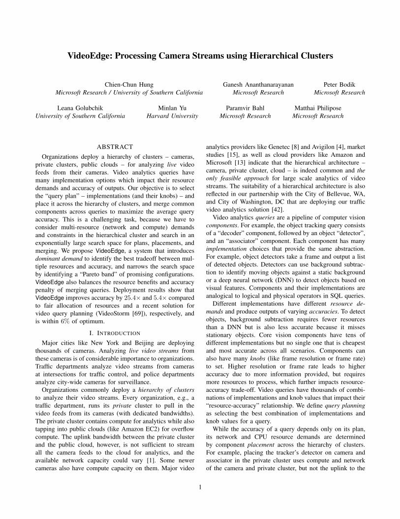
Figure 1: Hierarchical Video Analytics Architecture. Networklinks between cameras, private clusters, and the public cloudhave diverse bandwidths (represented by the width of thearrow). The compute at the locations also vary.

A. Hierarchical Clusters

Organizations with large deployment of cameras – e.g.,cities, police departments, or agriculture farms – typicallyuse a hierarchy of clusters (or locations, interchangeably)to process video streams [4], [8], [14], [62]. Figure 1 showsthat each organization (e.g., NYPD) runs private clusters thatpull video from their cameras.Compute hierarchy: Compute capacities at the privateclusters vary significantly from just a handful of cores (asin a small farm) to hundreds of cores (as in New YorkCity [14]), and can include GPUs or other hardware DNNaccelerators. Newer cameras themselves contain computecapacity [5] for video analytics and organizations may alsotap into the public cloud like Amazon EC2 and MicrosoftAzure for compute.Network: Connectivity between the cameras and privateclusters (via cellular, wireless [70] or fiber links) is a crucialresource. The bandwidth required to support a single camerastream ranges from a few hundred Kb/s to many Mb/s formulti-megapixel cameras. We can control the bitrate of thevideo stream by configuring the resolution and frame ratedirectly on the camera. Typically, the uplink from privateclusters to the public cloud is a few tens of Mb/s [1]and supports streaming only a small fraction of camerastreams to the cloud (per our conversations with Avigilon [4]and Genetec [8], leaders in video analytics solutions). Inrural deployments, such as cameras for monitoring cropsin farms [62], uplink Internet connectivity is even morerestricted and expensive.

Trends of increased compute availability on the “edge”(on cameras and private clusters) and bandwidth scarcityin reaching the cloud [53] has made the “intelligent edge”model a strong focus for many large industry players likeMicrosoft and Amazon in their IoT product offerings [13].Because of high bandwidth requirements, utilizing the com-pute on the hierarchy of edges is the only feasible approachfor processing live videos at scale [15]. Our discussions withmany traffic jurisdictions in the USA that we partner with,also indicate their keenness on utilizing compute on theircameras to reduce the cloud expenditure.

B. Implementations for Vision Primitives

Video processing often involves core vision primitives– object detection, objects association across frames, andrecognition of object class – each with many implemen-tation choices. A common approach to object detection isto extract moving objects using background subtraction orusing DNNs such as YOLO [51]. There are over 40 differentalgorithms in the background subtraction library [7]. To as-sociate objects across frames, one can use different metricssuch as color histograms, or the SIFT [11] or SURF [12]features. The VOT 2016 object tracking challenge has 70different associators [16]. The ImageNet object recognitionchallenge [10] has up to 80 different recognizers. Finally,for the primitives with DNN implementations, compressiontechniques [33] can create tens of efficient variants from anybaseline DNN.

Each implementation has different resource demands andaccuracy because it targets different conditions (e.g., light-ing, camera angle, object sizes) and based on differentstatistical assumptions. The YOLO [51] object detector isaccurate in scenes with just a few big objects but nototherwise, while background subtraction based detectors, amuch cheaper technique, only works for moving objects ina fixed camera. In choosing associator implementations, theexpensive SIFT features work well even in the presenceof shadows, while the much cheaper color histogram iswell-suited to track turning objects because the colors willlikely be the same no matter their angle to the camera.Further, tracking a single rigid object (e.g., a car) on a fixedcamera is simple, while tracking people in a dense crowdrequires more sophistication. For these reasons, there is noimplementation that is universally accurate and cheapest forall conditions.

Query plans: A video processing query typically includesmultiple core vision primitives. Given that each primitivehas tens of implementations to choose from and can alsobe configured with various knobs (e.g., different videoresolutions or frame rates) [69], there are often hundredsor thousands of query plans – choice of implementationsand knobs.

Common vision components across queries: Organizationsoften run tens of queries on each camera stream such ascounting of various object types (cars, buses, trucks, SUVs,pedestrians), traffic violations like jay walking, and collisionanalysis between vehicles and bicycles, with our trafficvideo analytics partners [42]. These queries reuse the samecore primitives like detectors, associators, and recognizers.Thus, we need to optimize across queries and allow mergingthese common components to substantially reduce resourcedemands. However, merging also constrains the commoncomponent to have the same plan (implementation choice)and placement across the many queries.

3

0

0.25

0.5

0.75

1

0 1 2 3

Accu

racy

CPU (Detector + Associator)

(a) Accuracy vs. Cores

00.25

0.50.75

1

0 1 2 3 4 5

Accu

racy

Network rate (Mb/s) (Detector + Associator)

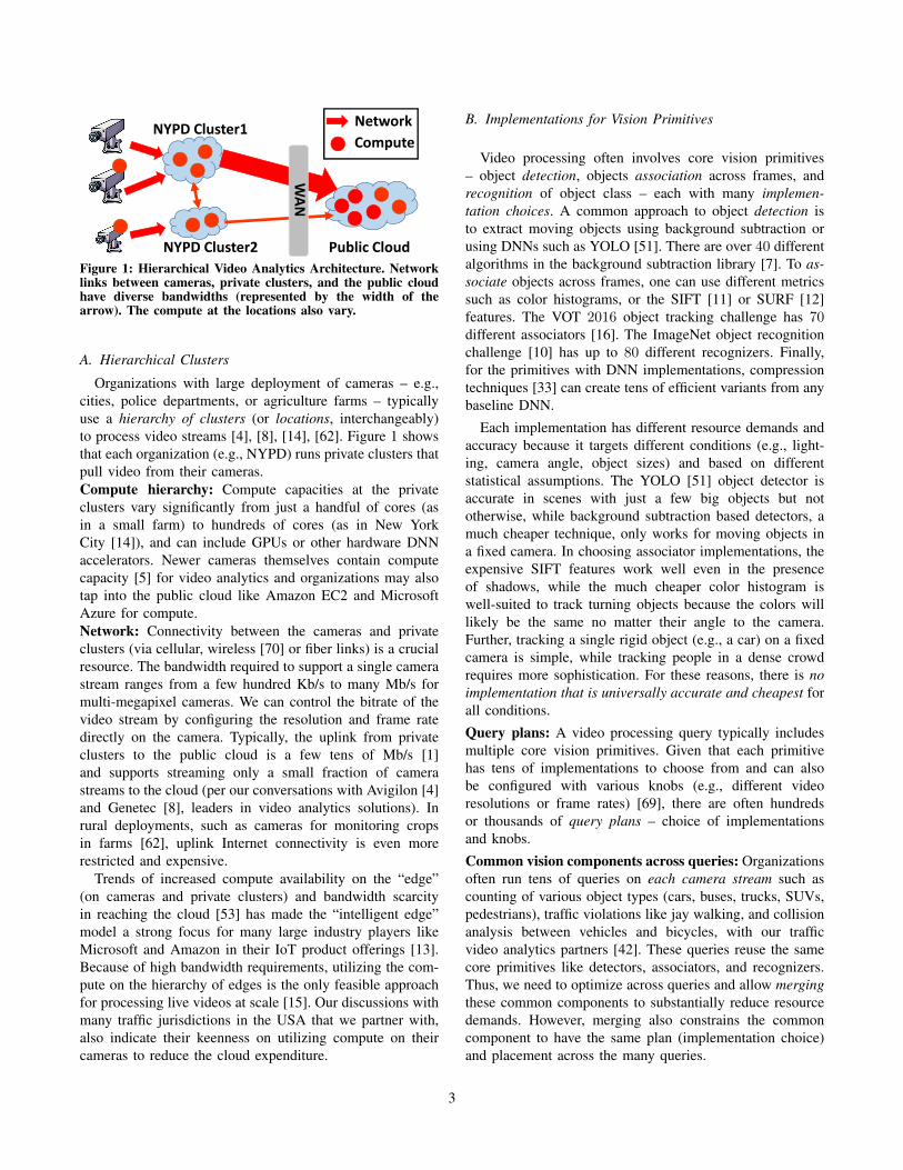
(b) Accuracy vs. Network ratesFigure 2: Resource-accuracy profile of the tracker.

0

1

2

camera

stream rate

detector

CPU

detector

output rate

associator

CPU

associator

output rate

dem

and [

core

s o

r M

bps]

A B

Figure 3: Network and CPU demands of the camera and thetwo modules in the tracker pipeline for two different plans,both with accuracy 0.73− 0.75.

C. Resource-accuracy Trade-off

Different query plans have different CPU and networkdemands, and accuracy. We illustrate this using an objecttracker, which is a key building block for many videoqueries. An object tracker consists of two components: adetector detects objects in each frame of the video, while anassociator associates those objects to existing tracks or startsnew tracks. We use a representative traffic camera streamfrom a large US city with an original bitrate of 3 Mb/s at30 frames/second to compare 300 query plans that vary theresolution, frame rate and different implementations of thedetector and associator.Resource demand vs. accuracy: To compute accuracy,we compare our output tracks against the ground truthobtained via crowd-sourcing. An object’s track is a time-ordered sequence of boxes across frames, and in each framewe calculate the F1 score ∈ [0, 1] (the harmonic mean ofprecision and recall [60]) between the box in the groundtruth and the track generated by the tracker. When computingF1 score for a query result with lower frame rate, i.e.,sampling, we compare the results on the sampled framewith its corresponding frame in the ground truth. We defineaccuracy of the track as the average of the F1 scores acrossall the frames. Figure 2 reports the trade-off between theresource demands – CPU and network demand (sum ofoutput data rate of the detector and associator but excludethe input stream rate) – against accuracy. The wide rangeof demands and accuracies is caused by differences inimplementations (§II-B). Factors like the light (shadows orovercast) and direction of the car (straight or making a turn)affect the accuracy.

0.40.50.60.70.8

1 10 100 1000

Object (Server GPUs) Object (Mobile GPUs)

Scene (Server GPUs) Scene (Mobile GPUs)

Face (Server GPUs) Face (Mobile GPUs)

GPU Cycles (Millions)

Accu

racy

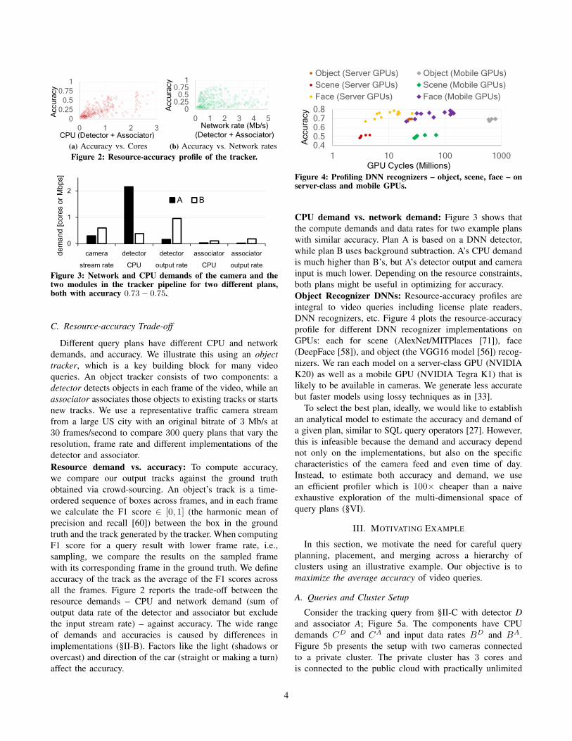
Figure 4: Profiling DNN recognizers – object, scene, face – onserver-class and mobile GPUs.

CPU demand vs. network demand: Figure 3 shows thatthe compute demands and data rates for two example planswith similar accuracy. Plan A is based on a DNN detector,while plan B uses background subtraction. A’s CPU demandis much higher than B’s, but A’s detector output and camerainput is much lower. Depending on the resource constraints,both plans might be useful in optimizing for accuracy.Object Recognizer DNNs: Resource-accuracy profiles areintegral to video queries including license plate readers,DNN recognizers, etc. Figure 4 plots the resource-accuracyprofile for different DNN recognizer implementations onGPUs: each for scene (AlexNet/MITPlaces [71]), face(DeepFace [58]), and object (the VGG16 model [56]) recog-nizers. We ran each model on a server-class GPU (NVIDIAK20) as well as a mobile GPU (NVIDIA Tegra K1) that islikely to be available in cameras. We generate less accuratebut faster models using lossy techniques as in [33].

To select the best plan, ideally, we would like to establishan analytical model to estimate the accuracy and demand ofa given plan, similar to SQL query operators [27]. However,this is infeasible because the demand and accuracy dependnot only on the implementations, but also on the specificcharacteristics of the camera feed and even time of day.Instead, to estimate both accuracy and demand, we usean efficient profiler which is 100× cheaper than a naiveexhaustive exploration of the multi-dimensional space ofquery plans (§VI).

III. MOTIVATING EXAMPLE

In this section, we motivate the need for careful queryplanning, placement, and merging across a hierarchy ofclusters using an illustrative example. Our objective is tomaximize the average accuracy of video queries.

A. Queries and Cluster Setup

Consider the tracking query from §II-C with detector Dand associator A; Figure 5a. The components have CPUdemands CD and CA and input data rates BD and BA.Figure 5b presents the setup with two cameras connectedto a private cluster. The private cluster has 3 cores andis connected to the public cloud with practically unlimited

4

Object

Associator

[A]

Object

Detector

[D]Camera

BDBA

(a) Object Tracker Pipeline

Public CloudPrivate

Cluster

Compute

3 cores

Network

3 Mb/s

1

2

(b) Hierarchical Setup

Query

PlanBD BA CD CA Accuracy

Q1080p 3 1.5 3 3 0.9

Q480p 1.5 1 2 2 0.6

Q240p 1 0.5 0.5 0.5 0.2

(c) Query plans for the tracker

CD

1080p BD

480p

BA

1080p

3 Mb/s3 cores

CPU Network

1.5

1.5

(d) Utilization at private clusterfor best plans & placement

Figure 5: Illustrative Example with two tracker queries (Fig.(a)) running on a hierarchical setup (Fig. (b)). Both queries Q1

and Q2 have the same profile of plans (Fig. (c)).

compute capacity; for ease of illustration, we assume nocompute on the camera. The private cluster has a 3 Mb/slink to the public cloud and each camera has a dedicated 3Mb/s link to the private cluster.

We consider three queries to execute on each of thecamera streams – car counting, jay walking, and collisionanalysis. All the three queries build atop a tracker (detector→ associator, Figure 5a). To simplify the example, weassume that the query components that consume the associ-ator’s output to count cars, identify jay walkers and analyzecollisions consume negligible resources, and hence all theresource consumption is by the detector and associatorcomponents. The accuracy of the tracker’s output directlytranslates to the accuracy of the outputs of each of thesequeries.

Assume that the only knob we control in the query plans isthe frame resolution (which is configurable on the camera).Figure 5c shows the profile of the query plans. Both theaccuracy of the tracker’s outputs as well as its resourcedemands (data rates BA and BD, and CPU demands CD

and CA) drop with the frame resolution.

B. Planning, Placement, and Merging

Each query has three query plan options (1080p, 480p,or 240p) and three placement options: (a) both componentsin the private cluster, (b) detector in the private cluster andassociator in the cloud, (c) both in the cloud.1 Hence, in ourexample, each query has 9 configurations (combinations ofquery plans and placements).Merging: The only choice to run the six queries (threequeries off each camera stream) is picking the 240p resolu-tion for each query, Q240p, leading to an average accuracyof only 0.2. Any other combination of query plans makes

1Placing the detector in the cloud and associator in the private cluster isclearly wasteful and we do not consider this placement option.

AssociatorDetectorCar

Counter

AssociatorDetector Jay

Walkers

AssociatorDetector

Car

Counter

Jay

Walkers

Collision

AnalysisFigure 6: Merging the detector and associator of the “carcounter”, “jay walker”, and “collision analysis” queries on thesame camera stream.

it infeasible to place the components due to insufficientcompute or network capacity. However, in contrast to thecurrent practice of treating these queries independently, wecan merge their common components and run only oneinstance of the detector and associator for each camera’svideo stream, see Figure 6. Merging saves us network andcompute; we avoid redundant streaming from the cameraand execution of the components.

Planning and placement: For each of the two mergedtracking pipelines, Q1 and Q2, picking 1080p resolutionmaximizes the accuracy (Q1

1080p and Q21080p), but we cannot

pick 1080p for both simultaneously because it is infeasibleto place the components. Placing all the components in thecloud requires a bandwidth of 6 Mb/s (BD + BD) againstthe available 3 Mb/s. If one tracker’s detector (needing 3cores) is placed in the private cluster (capacity of 3 cores),the network link of 3 Mb/s between the private cluster andthe cloud is still insufficient to support the aggregate datarate of 4.5 Mb/s (BD + BA for 1080p). At the same time,the private cluster’s compute is insufficient to support all thecomponents locally.

Picking Q1480p and Q2

1080p (or Q11080p and Q2

480p) is feasibleand leads to the best average accuracy of (0.9 ∗ 3 + 0.6 ∗3)/6 = 0.75. However, this is feasible only if we place thedetector of Q2

1080p in the private cluster and its associatorin the cloud, while forwarding Q1

480p’s camera stream upto the cloud for executing both its detector and associator.Figure 5d shows the resulting utilizations at the privatecluster. This illustrates the need to determine query plans andplacements jointly, across all queries, and consider multipleresources (unlike current database optimizers [2], [20]).

Note that while the above example for merging wassimplified, the decision is non-trivial in practice. This isbecause we need to select the same plan for the mergedcomponents which may often lead to conflicting accuracies.Car counting works better with background subtractionbased object detector, while we need a DNN detector toidentify pedestrians for jay walking. We have to resolve suchmerging conflicts and ensure that the best merged plan is notoverly resource intensive.

5

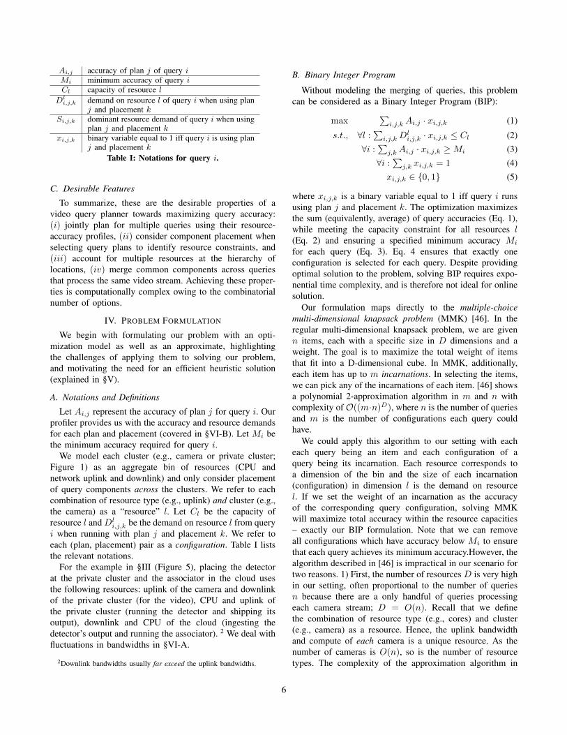
Ai,j accuracy of plan j of query iMi minimum accuracy of query iCl capacity of resource l

Dli,j,k demand on resource l of query i when using plan

j and placement kSi,j,k dominant resource demand of query i when using

plan j and placement kxi,j,k binary variable equal to 1 iff query i is using plan

j and placement kTable I: Notations for query i.

C. Desirable Features

To summarize, these are the desirable properties of avideo query planner towards maximizing query accuracy:(i) jointly plan for multiple queries using their resource-accuracy profiles, (ii) consider component placement whenselecting query plans to identify resource constraints, and(iii) account for multiple resources at the hierarchy oflocations, (iv) merge common components across queriesthat process the same video stream. Achieving these proper-ties is computationally complex owing to the combinatorialnumber of options.

IV. PROBLEM FORMULATION

We begin with formulating our problem with an opti-mization model as well as an approximate, highlightingthe challenges of applying them to solving our problem,and motivating the need for an efficient heuristic solution(explained in §V).

A. Notations and Definitions

Let Ai,j represent the accuracy of plan j for query i. Ourprofiler provides us with the accuracy and resource demandsfor each plan and placement (covered in §VI-B). Let Mi bethe minimum accuracy required for query i.

We model each cluster (e.g., camera or private cluster;Figure 1) as an aggregate bin of resources (CPU andnetwork uplink and downlink) and only consider placementof query components across the clusters. We refer to eachcombination of resource type (e.g., uplink) and cluster (e.g.,the camera) as a “resource” l. Let Cl be the capacity ofresource l and Dl

i,j,k be the demand on resource l from queryi when running with plan j and placement k. We refer toeach (plan, placement) pair as a configuration. Table I liststhe relevant notations.

For the example in §III (Figure 5), placing the detectorat the private cluster and the associator in the cloud usesthe following resources: uplink of the camera and downlinkof the private cluster (for the video), CPU and uplink ofthe private cluster (running the detector and shipping itsoutput), downlink and CPU of the cloud (ingesting thedetector’s output and running the associator). 2 We deal withfluctuations in bandwidths in §VI-A.

2Downlink bandwidths usually far exceed the uplink bandwidths.

B. Binary Integer Program

Without modeling the merging of queries, this problemcan be considered as a Binary Integer Program (BIP):

max∑

i,j,k Ai,j · xi,j,k (1)

s.t., ∀l :∑

i,j,kDli,j,k · xi,j,k ≤ Cl (2)

∀i :∑

j,k Ai,j · xi,j,k ≥Mi (3)∀i :

∑j,k xi,j,k = 1 (4)

xi,j,k ∈ {0, 1} (5)

where xi,j,k is a binary variable equal to 1 iff query i runsusing plan j and placement k. The optimization maximizesthe sum (equivalently, average) of query accuracies (Eq. 1),while meeting the capacity constraint for all resources l(Eq. 2) and ensuring a specified minimum accuracy Mi

for each query (Eq. 3). Eq. 4 ensures that exactly oneconfiguration is selected for each query. Despite providingoptimal solution to the problem, solving BIP requires expo-nential time complexity, and is therefore not ideal for onlinesolution.

Our formulation maps directly to the multiple-choicemulti-dimensional knapsack problem (MMK) [46]. In theregular multi-dimensional knapsack problem, we are givenn items, each with a specific size in D dimensions and aweight. The goal is to maximize the total weight of itemsthat fit into a D-dimensional cube. In MMK, additionally,each item has up to m incarnations. In selecting the items,we can pick any of the incarnations of each item. [46] showsa polynomial 2-approximation algorithm in m and n withcomplexity of O((m·n)D), where n is the number of queriesand m is the number of configurations each query couldhave.

We could apply this algorithm to our setting with eacheach query being an item and each configuration of aquery being its incarnation. Each resource corresponds toa dimension of the bin and the size of each incarnation(configuration) in dimension l is the demand on resourcel. If we set the weight of an incarnation as the accuracyof the corresponding query configuration, solving MMKwill maximize total accuracy within the resource capacities– exactly our BIP formulation. Note that we can removeall configurations which have accuracy below Mi to ensurethat each query achieves its minimum accuracy.However, thealgorithm described in [46] is impractical in our scenario fortwo reasons. 1) First, the number of resources D is very highin our setting, often proportional to the number of queriesn because there are a only handful of queries processingeach camera stream; D = O(n). Recall that we definethe combination of resource type (e.g., cores) and cluster(e.g., camera) as a resource. Hence, the uplink bandwidthand compute of each camera is a unique resource. As thenumber of cameras is O(n), so is the number of resourcetypes. The complexity of the approximation algorithm in

6

[46] thus becomes O((m·n)n), which is exponential with thenumber of queries and is too slow in practice. 2) Second, thedescription so far ignores merging of queries. We can extendthe formulation to handle query merging as follows. Onlythe queries that process video from the same video streamcan merge; we thus logically group all queries on the samestream into super-queries and enumerate all the differentconfigurations (or incarnations) of each super-query as allcombinations of possible ways to merge these queries, theirconfigurations and placement. However, this would make mexponential in the number of queries per stream and numberof modules in the query DAGs, again making the algorithmtoo slow to use in practice.

We are unaware of other (approximate) algorithms withpolynomial complexity that apply in this setting. Instead, wedevelop an efficient heuristic next in §V.

V. VideoEdge’S VIDEO QUERY OPTIMIZATION

VideoEdge is a video query optimization framework thatjointly optimizes all queries to maximize the average queryaccuracy within the available resources. Specifically, weplan for each query (pick its implementations and knobs),place components of the query across the hierarchy ofclusters, and merge identical components of queries thatprocess the same stream to save resources.

A. Dominant Resource Demand

VideoEdge’s profiler (§VI-B) estimates demands (Dli,j,k)

and accuracies (Ai,j) for each query configuration. To decidebetween two configurations c0 and c1, we need to comparetheir accuracies and resource demands. Is c1 improving theaccuracy enough for the amount of additional resources itconsumes? However, because the queries utilize multipleresources across many clusters (see §IV-A), it is tricky tocompare resource demands.

Therefore, we define a dominant demand which convertsdemand for multiple resources into a single value; specif-ically, the dominant demand of placement k of plan j forquery i Si,j,k = maxlD

li,j,k/Cl. S is a scalar that measures

the highest fraction of resources l needed by the query acrossresource types (CPU, network) and clusters (camera, privatecluster, cloud).

A nice property of the dominant demand metric is that,by normalizing the demand D relative to the capacity C ofthe clusters, it avoids lopsided drain of any single resourceat any cluster. As a critical insight, if the system runs outof network bandwidth between two clusters, no more datacan go through them and their remaining CPU resources arewasted. Also, by being dimensionless, it easily extends tomultiple resources, akin to DRF [31]. While we also con-sidered defining Si,j,k using sum of the resource utilizations(∑

l instead of maxl) or just the absolute demands, theyperformed worse in our evaluations.

1: U . Set of all (i, j, k) tuples of all queries i and theavailable plans j and placements k

2: pi . Plan assigned to query i3: ti . Placement assigned to query i4: for all query i do5: (pi, ti) = argmin(j,k) Si,j,k . Agg. demand S, §V-A

6: for each resource l: update Rl

7: while U 6= ∅ do8: U’ ← U −{(i, j, k)where ∃l : Rl < Dl

i,j,k}9: remove (i, j, k) from U if Ai,j,k ≤ Ai,pi,ti

10: (i?, j?, k?) = argmaxi,j,k∈U′ Ei(j, k)11: pi? ← j?, ti? ← k?

12: for each resource l: update Rl based on Dli?,pi? ,ti?

Figure 7: Pseudocode for VideoEdge’s heuristic.

B. Greedy Heuristic

We first describe our heuristic without considering merg-ing and then incorporate it in §V-C. To maximize averageaccuracy, it is crucial to efficiently utilize the availableresources. We employ the intuitive principle of allocatingmore resources to queries that can achieve higher accuracyper unit resource allocated compared to other queries. Toachieve this, we use an efficiency metric that relates theaccuracy to the dominant demand of the query.

Our heuristic starts with assigning the configuration withthe lowest dominant resource demand to each query andgreedily considers incremental improvements to the queries.3 When considering switching query i from its current planj and placement k to another plan j′ and placement k′,we define the efficiency of this change as the improvementin accuracy normalized by the required additional demand.Specifically:

Ei(j′, k′) =

Ai,j′ −Ai,j

Si,j′,k′ − Si,j,k

Defining Ei(j′, k′) in terms of the “delta” in both accu-

racy and demand turns out to be the most suited to ourgradient-based search heuristic. It outperformed alternatedefinitions that just used only the new values, e.g., onlyAi,j′ and/or Si,j′,k′ in our evaluations.

Figure 7 shows the pseudocode. U represents the set ofall (i, j, k) tuples of all queries i, the available plans j, andplacements k. The objective is to assign to each query i, aplan pi and placement ti; lines 1 − 3. It first assigns eachquery i the plan j and placement k with the lowest dominantdemand Si,j,k (lines 4−5). After that, it iteratively searchesacross all plans and placements of all queries and selectsthe query i? (and the corresponding plan j? and placementk?) with the highest efficiency (lines 7−12). Line 9 ensuresthat we only consider configurations that increase accuracy.It switches query i? to new plan j? and placement k?,and repeats until no query can be upgraded (either due to

3We only consider plans j with accuracy Ai,j ≥ Mi.

7

insufficient remaining resources, or no available plans withhigher accuracy).

In each iteration, we only consider configurations that fitin the remaining resources Rl by constructing U ′ (line 8).Note that we cannot remove such infeasible configurationsfrom U completely because they might become feasiblelater as the heuristic moves components across clusters bychanging configurations of queries.

A subtle aspect is that in each iteration, we remove thoseoptions from U that reduce a query’s accuracy relative toits currently assigned plan and placement (line 9). Suchan explicit removal helps because even though the changein accuracy of the removed options would be negative,those options may also have negative difference in dominantutilization (Si,j,k), thus making the efficiency positive andpotentially high.

Note that our heuristic can also work with other perfor-mance goals. For example, if each query has the requirementof minimum accuracy to be useful, our proposed heuristiccan first focus on getting all queries to a configuration thatmeets minimum accuracy before further improving overallaccuracy by selecting other configurations with higher accu-racy. Our heuristic can also work to achieve fairness acrossqueries: each iteration improves for the query with minimumaccuracy, until the resources are depleted.

The computational complexity of our heuristic withoutmerging is O((m · n)2). There are at most n ·m iterationsbefore the proposed heuristic terminates since each iterationremoves at least one configuration from consideration andthere are total n · m configurations. In each iteration, atmost n ·m configurations are explored, therefore the overalltime complexity is bounded by (m ·n)2. This is much moreefficient than [46] (§IV-B).

Note that we do not change the plan and placement of therunning queries in the system while the heuristic is runningbut only when all its iterations complete.

C. Merging Peer Queries

When there are multiple queries processing the samecamera feed with common prefix in their pipeline, we havethe opportunity to eliminate running redundant components.We refer to such queries as a peer set. Figure 6 shows anexample of peer set of queries. The directional car countingquery in traffic video uses a detector component for iden-tifying the vehicle, then a mapper component for keepingtrack of the same vehicle, and finally a counter componentto record the number of vehicles per direction. Anomalydetections also rely on an object detector component and amapper component to understand trajectories and to identifyanomalous behaviors. Since both queries require the detectorand mapper components, running only one copy of thesecomponents can save resources (Figure 6) which in turn canbe used to upgrade other queries’ plans. We call this asmerging.

Challenges: Despite the obvious resource benefits of merg-ing, the decision is non-trivial. Merging two peer queriesprocessing the same camera feed with common componentsis not always beneficial to their accuracies. This is because,the merged components have to be assigned common im-plementations and knob values. However, a query plan thatachieves good accuracy for one query may not do so for theother query. When counting cars and humans in the samecamera stream, different implementations of detectors andmappers are better suited. A background subtraction baseddetector and distance based mapper are better suited forcars. On the other hand, humans, owing to their smaller sizeare often missed by a background subtracter and require aricher SIFT metric for mapping. Hence, the decisions onmerging need to contend with such conflicts. Even whenthere are no conflicts on accuracy, picking the plan withthe common maximum accuracy might not be optimal asit might be too resource-intensive. Furthermore, whether tomerge the peer queries or not depend not just on the overallaccuracy they can achieve, but also depend on the availableresources and, most importantly, the trade-off between them.While merging peer queries could reduce resource usage,given sufficient resources, some of the peer queries mayend up having its own isolated module pipeline to gainbetter aggregate quality. A key question in merging peerqueries is deciding the implementation and knobs for themerged components. In addition, the decision of mergingis not just for the peer queries involved, but should alsoconsider the aggregate quality for all queries in the systemas the planning and placement of other queries would alsobe affected. Finally, the possible merging combinations growexponentially for a peer set of z queries (any subset ofqueries in a peer set can be merged). Jointly performingplanning, placement and merging is markedly different thanmulti-query optimizers in databases [30], [54].

To reduce the search space, we make two simplifyingassumptions when considering merging: (a) we either mergeall the common components or nothing at all. For theexample in Figure 6, we either merge both the detector andassociator or neither of them; we do not consider mergingonly the detector.Consider partial merging provides moreflexibility, yet it would increase the complexity significantly.Exploring more merging potions at reasonable overheads ispart of our future work. (b) we avoid searching throughall possible plans for the components that are not common(“counter”, “jay walker” and “collision” components inFigure 6) and use their plans from the previous iterationof the heuristic. The distinct components in vision queriesusually tend to not have many choices in their plans, andhence assumption (b) does not hurt our solution.

To realize merging peer queries, we make the followingchange to line 10 of Figure 7. When considering switching toconfiguration (p?i , t

?i ) of query i?, we also consider merging

this query with all subsets of its peer queries. Let R be one

8

0

0.2

0.4

0.6

0.8

1

0 0.2 0.4 0.6 0.8 1Resource Demand

Accu

racy

Figure 8: Illustration of Pareto band (shaded) for a singlequery. Note that for each accuracy (plan), there is a horizontalstripe of placement options with different demands.

of the subsets of i?’s peer queries. We merge all queries in Rwith i and apply the (p?i , t

?i ) configuration to all components

in i?. Any remaining components in the merged query (thatare not in i?) remain in their current plan and placement.For each such merged query, we compute the efficiencymetric E relative to all peer queries of i?, i.e., ratio ofthe aggregate increase in accuracy to the aggregate increasein the resource demand. The computational complexity ofour heuristic, after incorporating merging queries, becomesO((n·m)2 ·2z), in which z is the number of queries in a peerset: for each configuration considered in each iteration, theexploration is extended to consider all 2z possible subsetsof a query’s peer queries. 4

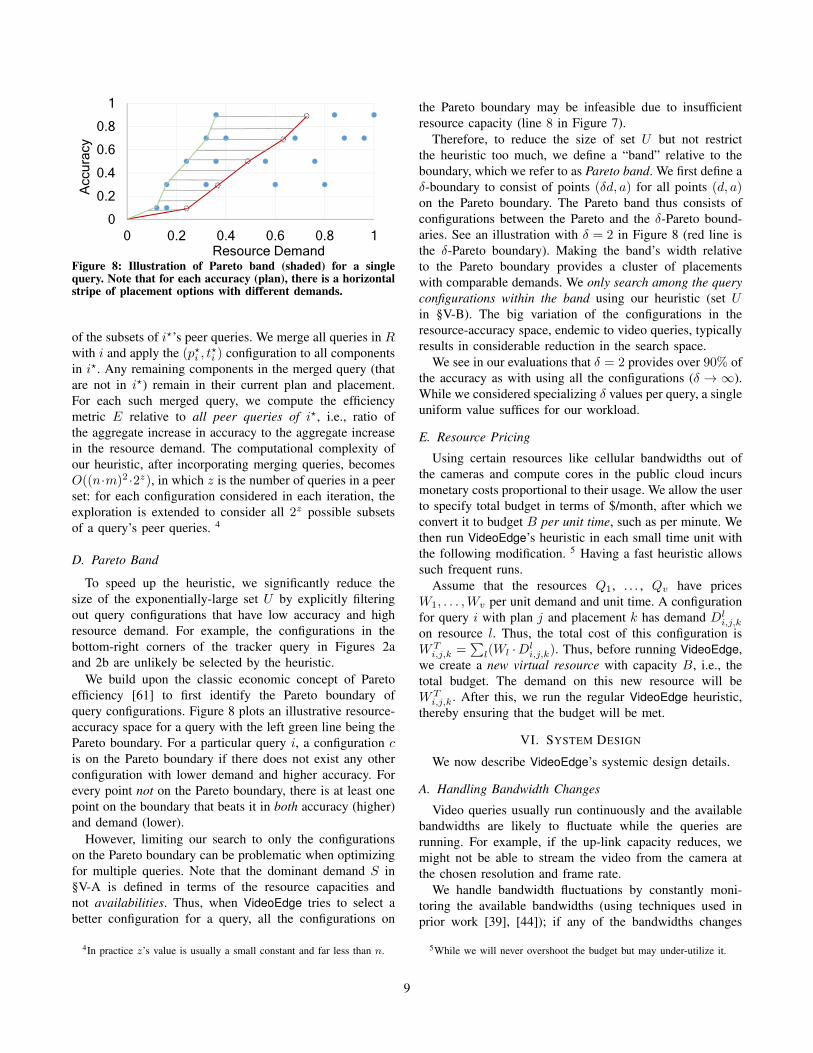
D. Pareto Band

To speed up the heuristic, we significantly reduce thesize of the exponentially-large set U by explicitly filteringout query configurations that have low accuracy and highresource demand. For example, the configurations in thebottom-right corners of the tracker query in Figures 2aand 2b are unlikely be selected by the heuristic.

We build upon the classic economic concept of Paretoefficiency [61] to first identify the Pareto boundary ofquery configurations. Figure 8 plots an illustrative resource-accuracy space for a query with the left green line being thePareto boundary. For a particular query i, a configuration cis on the Pareto boundary if there does not exist any otherconfiguration with lower demand and higher accuracy. Forevery point not on the Pareto boundary, there is at least onepoint on the boundary that beats it in both accuracy (higher)and demand (lower).

However, limiting our search to only the configurationson the Pareto boundary can be problematic when optimizingfor multiple queries. Note that the dominant demand S in§V-A is defined in terms of the resource capacities andnot availabilities. Thus, when VideoEdge tries to select abetter configuration for a query, all the configurations on

4In practice z’s value is usually a small constant and far less than n.

the Pareto boundary may be infeasible due to insufficientresource capacity (line 8 in Figure 7).

Therefore, to reduce the size of set U but not restrictthe heuristic too much, we define a “band” relative to theboundary, which we refer to as Pareto band. We first define aδ-boundary to consist of points (δd, a) for all points (d, a)on the Pareto boundary. The Pareto band thus consists ofconfigurations between the Pareto and the δ-Pareto bound-aries. See an illustration with δ = 2 in Figure 8 (red line isthe δ-Pareto boundary). Making the band’s width relativeto the Pareto boundary provides a cluster of placementswith comparable demands. We only search among the queryconfigurations within the band using our heuristic (set Uin §V-B). The big variation of the configurations in theresource-accuracy space, endemic to video queries, typicallyresults in considerable reduction in the search space.

We see in our evaluations that δ = 2 provides over 90% ofthe accuracy as with using all the configurations (δ → ∞).While we considered specializing δ values per query, a singleuniform value suffices for our workload.

E. Resource Pricing

Using certain resources like cellular bandwidths out ofthe cameras and compute cores in the public cloud incursmonetary costs proportional to their usage. We allow the userto specify total budget in terms of $/month, after which weconvert it to budget B per unit time, such as per minute. Wethen run VideoEdge’s heuristic in each small time unit withthe following modification. 5 Having a fast heuristic allowssuch frequent runs.

Assume that the resources Q1, . . . , Qv have pricesW1, . . . ,Wv per unit demand and unit time. A configurationfor query i with plan j and placement k has demand Dl

i,j,k

on resource l. Thus, the total cost of this configuration isWT

i,j,k =∑

l(Wl ·Dli,j,k). Thus, before running VideoEdge,

we create a new virtual resource with capacity B, i.e., thetotal budget. The demand on this new resource will beWT

i,j,k. After this, we run the regular VideoEdge heuristic,thereby ensuring that the budget will be met.

VI. SYSTEM DESIGN

We now describe VideoEdge’s systemic design details.

A. Handling Bandwidth Changes

Video queries usually run continuously and the availablebandwidths are likely to fluctuate while the queries arerunning. For example, if the up-link capacity reduces, wemight not be able to stream the video from the camera atthe chosen resolution and frame rate.

We handle bandwidth fluctuations by constantly moni-toring the available bandwidths (using techniques used inprior work [39], [44]); if any of the bandwidths changes

5While we will never overshoot the budget but may under-utilize it.

9

significantly for a certain amount of time, VideoEdge recom-putes its query optimizations. To minimize the disruption,we only recompute the query plan selection, while retainingthe current placement and merging decisions. In addition,the complete version of VideoEdge is periodically re-run toupdate the queries’ plans, placements and merges to ensurehigh resource utilization.

Also, we constantly run golden queries to monitor andcalibrate the accuracy of the queries. Our system can beconfigured to re-run the scheduling heuristic periodically(e.g., every 3 hours) to account for any dynamics andtherefore maintain high accuracy.

B. Resource-Accuracy Profiler

The profiler is a key component of VideoEdge. For eachquery, it estimates accuracy and per-component resourcedemands (CPU and bandwidths). Note that the profilerdoes not consider placement; the optimizer in §V jointlyincorporates placement with planning and merging.

The profiler estimates the query accuracy by running thequery on a labeled video dataset obtained via crowd-sourcingor by labeling the dataset using a “golden” query plan whichmight be resource-intensive but is known to produce highlyaccurate outputs. When a user submits a new query, we startprofiling it while submitting it to the scheduler with thedefault query plan.

Since a query can have thousands of plans which we haveto execute on the labeled videos, the main goal in profilingis to minimize the CPU demand of the profiler. We use twosimple tricks: (1) eliminating common sub-expressions bymerging multiple query plans and (2) caching intermediateresults of query components.

Assume that both components in the tracking query D →A have two implementations; D1, D2 and A1, A2. We thushave to profile four query plans: D1A1, D1A2, D2A1, andD2A2. If we run each plan separately, implementations D1

and D2 would run twice on the same video data. Instead,we merge plans of profiled queries, similar to §V-C, to avoidredundant runs.

While we could merge all the plans into one, executingthis would require large number of concurrent computeslots which might not be available. In such cases, weresort to caching of intermediate results. Note that whilecaching alone will eliminate redundant executions, it hasdramatically high requirement on storage space. In profilingthe tracker on a 5-minute traffic video, the storage space forcaching is 78× the size of the original video.

Hence, we assign a caching budget per query. We pref-erentially cache the outputs of those components that takelonger to generate. In addition, we also like to cache the out-puts of those components which are to be used more. Theseare components with many downstream components eachwith many implementations and knob choices. We encodethese in a metric for each intermediate result, M = n × T

S

where n is the number of times this output will be accessed,T is the time taken to generate the output, and S is thesize of the output. Our profiler uses the caching budget forintermediate outputs with higher value of the M metric.Benefit: For the tracking query, our profiler uses 100× fewerCPU cycles compared to exhaustive exploration of all plans.We use cache budget of 900MB per machine, which webelieve is practical in modern machines. On a 16-core ma-chine, our profiler took 10 minutes to complete, which couldbe parallelized across more machines. Such improvement inefficiency, allows us to run the profiler periodically and usethe most recent resource-accuracy profile in our optimizerin §V.

VII. EVALUATION

We evaluate VideoEdge with an Azure deployment em-ulating a hierarchy of clusters using representative videoqueries, and complement it using large-scale simulations.

1) VideoEdge outperforms state-of-the-art solutions byup to 25.4× better average accuracy, while beingwithin 6% of the optimal accuracy.

2) Merging queries with common component accountsfor an additional 1.6× better accuracy.

3) Searching only the configurations in the Pareto banddrops the heuristic’s running time by 80% while stillachieving ≥ 90% of the original accuracy.

A. Setup

Azure deployment. We use a 24 node Azure clusterto emulate a hierarchical setup; each node is a D3v2instance with 4 cores and 14GB of memory. Ten of thenodes are the “camera compute”; two cameras per node.The 20 cameras “play” feeds from 20 recorded streamsfrom many cities in the USA at their original resolutionand frame rate. Two nodes act as a private cluster. Eachcamera has a 600Kb/s link to the private cluster, resemblingthe bandwidths available today. The cloud consists of 12nodes with a 5Mb/s uplink from the private cluster. Thesebandwidths are based on measurements at our partner trafficjurisdictions at the City of Bellevue, WA and elsewhere.They are also consistent with recent studies from Akamai[1]. We also use simulations to evaluate larger settings undervarying resource capacities.

Video queries. We profile and evaluate using the fol-lowing queries: tracker, DNN object classifier (trained inadvance), car counter, and license plate reader – a typicalcombination of queries. The queries have 300, 20, 10, and30 query plans, respectively, from different implementationand knob choices. These queries are pre-defined in ourexperiments so that we can profile them to obtain theresource-accuracy profiles with various configurations. Eachquery has two components and among the three clusters inthe hierarchy there are six placement options per query: bothcomponents in the same cluster or each in a different cluster

10

(a) Small-scale Setting. (b) Comparison with Baselines. (c) Impacts of Merging.Figure 9: Improvement in Accuracy.

0

0.2

0.4

0.6

0.8

1

1 2 3 4 5Accu

racy

/ A

ccur

acy

of B

IP

Average Number of Queries Per Camera

VideoEdge w/o Merging VideoStormVideoSotrm_Random VideoStorm_CameraVideoStorm_Cluster VideoStorm_Cloud

Figure 10: Comparing VideoEdge to VideoStorm with differentplacement options

(we avoid placements that go “down” from the cloud).We use 200 video clips (each 5-minutes long) from manylocations and times of day, and thus generate 200 resource-accuracy profiles for our experiments. The groundtruth forthese video queries are obtained by manually labeling. Eachquery has 300 configurations; 5 resolution and 5 samplingrate values, 3 object detector implementations (two based onbackground subtraction and one on DNN) and 4 differenttracking metrics. Since there are 6 different placements forthe tracker query components, our heuristic considers 1800total configurations. Each experiment is run 5 times, and themedian result reported.

Baselines. We compare against four approaches.(1) Fair Allocation, since it is widely used in production

clusters [19], [34]. We extend the definition of fairness usedwithin a cluster ( 1

n of the resources in a cluster given nqueries) to multiple clusters by allocating 1

n of each resourcein each cluster. Within this fair allocation, each query picksthe configuration (query plan and placement) that achievesthe highest accuracy. 6

(2) Recent work on video analytics, VideoStorm [69],a single-cluster, single-resource video query planner. We

6While we considered using DRF [31] as our fair allocation baseline, theDRF algorithm is intertwined with component placement unlike a simplefair allocation. This is because, DRF requires the demand at each clustereven to define the dominant fair share, which in turn is a function ofplacement and not known beforehand.

use the aggregate CPU of all the clusters for its planning.Being a single-cluster solution, VideoStorm does not in-clude placements and may selects query configurations thatare supported by bandwidth capacity. We place its querycomponents starting in the cameras, and move on to placethem at private clusters if the cameras do not have sufficientcompute CPU resources, and eventually move to the cloudif both the cameras and the private clusters run out of CPUresources. Such placement method for VideoStorm may notbe ideal, but provides fair insights in comparison withoutdeviating from its design spirits. We also ensure that it avoidsinfeasible placements (e.g., insufficient network or computeresource). In our experiments we also compare VideoEdgeto VideoStorm with additional placement options.

(3) To compute the optimal plan and placement withoutmerging, we solve the BIP optimization (§IV-B) with theGurobi solver [9]. We compute the optimal results withmerging using brute-force computation.

Performance metric. Our performance metric is theaverage accuracy across all queries. We report the rel-ative improvement over the baseline; given accuracies ofVideoEdge and a baseline are Ac and Ab, we report Ac

Ab.

B. Improvement in Accuracy

We begin with presenting the improvement in accuracyusing our Azure deployment. We run the tracking queriesand assign them uniformly to the cameras; each camera runsa randomly chosen video from the 200 options. We compareagainst the two optimal strategies: 1) brute-force, whichconsiders merging but only scales to small deployments, and2) BIP, which does not consider merging but scales to ourdefault deployment.

First, we use the brute-force optimum in a small-scalesetting with just one camera, one private cluster, and cloudand vary the number of queries from two to four.7 Even atthis small scale with four queries, brute force takes 400 CPUdays to complete, compared to VideoEdge completing in 1.5CPU seconds. Figure 9a shows that, although the average

7To quantify gains from merging, we only include queries with the samecomponents, e.g., a detector and an associator.

11

accuracy decreases with more queries sharing the resources,VideoEdge achieves within 93%− 96% of optimum.

Next, we compare against the BIP optimum that does notconsider merging in our default-scale setting, see Figure 9b.We also include VideoEdge without merging since the base-lines do not merge queries. We make several observations.First, VideoEdge w/Merging constantly outperforms BIPwhen merging queries is possible (i.e., more than 1 queryper camera), and the gap increases as there are more queriesin the system. This suggests that VideoEdge’s considera-tion of merging queries plays a key role in VideoEdge’seffectiveness. Second, VideoEdge significantly outperformsVideoStorm and Fair Allocation and the gains increase as thenumber of queries increases: its accuracy is 5.4× and 25.4×better than VideoStorm and Fair Allocation, respectively,with 5 queries executing on every camera stream. Finally,without the consideration of merging queries, the accuracyof VideoEdge w/o Merging is within 94% of BIP evenwith the increasing number of queries in the system, and is3.3× and 15.7× better than VideoStorm and Fair Allocation,respectively, with 5 queries executing on every camerastream.

Figure 10 further compares VideoEdge to VideoStormwith different placement options. The additional placementoptions for VideoStorm in this experiment include: (a)placing all query components in the cameras (VideoStorm-Camera), (b) placing all query components in the privateclusters (VideoSotrm-Cluster), (c) placing all query com-ponents in the cloud (VideoStorm-Cloud), and (d) placingquery components randomly across the locations, whilemaking sure it does not exceed bandwidth capacity. Theresults suggest that VideoEdge outperforms VideoStorm inall the cases, including the hierarchical placement option wedescribed earlier. We use the hierarchical placement optionfor VideoStorm in our experiments since it provides the bestaccuracy for VideoStorm. From the experiments in Figure 10we learn that “retrofitting” query placement after query plansare selected is less beneficial as compared to VideoEdge’sapproach of making joint decision on the two factors.Merging conflicts. While merging queries can reduce re-source usage and improve accuracy by 1.6× (see Figure 9b),recall that it can lead to “conflicts” between queries whenthey have different resource-accuracy profiles, thus needingus to weigh the resource gains from merging against any lossin accuracy. To highlight this, we compare against a “MergeEverything” heuristic that merges all possible componentswithout considering conflicts, see Figure 9b; it achievesmuch smaller gains.

C. Characterizing the Gains

Next, we characterize VideoEdge’s gains against the base-lines in the scenario of no-merging consideration.Resource efficiency. Figure 11a presents the distributionof the absolute query accuracies with the “2-queries-per-

0

0.2

0.4

0.6

0.8

1

0 20 40 60 80 100

Accu

racy

CDF (%)

BIP VideoEdge

0

0.2

0.4

0.6

0.8

1

0 20 40 60 80 100

Dom

inan

tDem

and

of

Chos

en C

onfig

urat

ion

CDF (%)

VideoStorm Fair

(a) Accuracy.

0

0.2

0.4

0.6

0.8

1

0 20 40 60 80 100

Acc

urac

y

CDF (%)

Optimal CascadeBIP

0

0.2

0.4

0.6

0.8

1

0 20 40 60 80 100

Dom

inan

tDem

and

of

Chos

en C

onfig

urat

ion

CDF (%)

VideoStorm Fair

(b) Dominant Demand.Figure 11: CDF of Accuracy And Dominant Demand.

Figure 12: Choice of placements for components.

camera” setting. VideoEdge’s CDF closely matches BIP,which shows that VideoEdge’s greedy heuristic search inthe Pareto band is near-optimal even at a per-query level,not just in aggregate. The key to VideoEdge’s performanceis effective utilization of resources. The CPU and networkutilizations are all above 85%, thus showing the effectivenessof VideoEdge in balancing the load across clusters andavoiding bottlenecks. This is mainly due to our metric ofdominant demand (§V-A) that prevents any single resourcefrom being disproportionately utilized. This is supported byFigure 11b that shows that the queries’ dominant demandsachieved by VideoEdge are significantly higher than with fairallocation and VideoStorm, and similar to BIP, thus leadingto higher utilizations and accuracies.Placement decisions. Figure 12 presents the distribution ofthe six options for placing the detector and associator. For93% of queries, VideoEdge places both components of aquery at the same location, i.e., ”Camera-Camera”, ”Cluster-Cluster”, and ”Cloud-Cloud”. As a result, the intermediatedata between the components does not use the networkbetween clusters, thus avoiding contention. VideoStorm’srandom placement strategy places 23% of the query com-ponents across clusters which adversely impacts its queryplans and accuracies.

Next, we evaluate VideoEdge with constrained queryplacement – like in many production video analytics de-ployments – to one level in the hierarchy. All the queriesrun (i) on their corresponding camera, (ii) in the privatecluster, or (iii) in the cloud. Figure 13 shows the ratioof VideoEdge’s accuracies (without merging) over each of

12

Figure 13: VideoEdge’s gains over restricted placements.

the three constrained approaches. Note that each queryconfiguration could have different knob values, e.g., videoresolution, which requires decoding differently at the cam-eras. Hence the same video source could be transmitted withmultiple streams each with different decoding scheme, andthis depends on the number of queries running over the samecamera. As the number of queries (per camera) increases,the compute or network resources become saturated and theycannot support the queries at high accuracies. For example,with just one query per camera, we can stream all video tothe cloud and process it there; however, as the load increases,this becomes harder and VideoEdge can run the querieswith up to 3× higher accuracy. We achieve the largestgains against the camera-only constraint because the camerashave the least compute available. These results highlight thevalue in jointly utilizing the hierarchy of clusters for videoanalytics.Gains by query type. We also evaluate a wider (equal)mix of query types – object tracker, DNN classifier, carcounter, license plate reader – in our simulator. We profilethese queries using our profiler (§VI-B) and feed theseto the simulator. The cluster settings are similar to thedeployment. We measure that the license plate reader andcar counter are farther from the optimal (87% of BIP) unlikethe other two that are near-optimal. This is explained bythe resource-accuracy profiles of the queries. The licenseplate reader and car counter, beyond a certain accuracy,have inefficient profiles (see §V-B). The additional resourcesneeded to improve their accuracy are higher compared tothe object tracker and DNN queries which have many moreefficient configurations. As a result, our heuristic assignsmore resources to the latter two.

D. Scalability with Pareto Band

In §V, we narrow down our search space by using a Paretoband of promising configurations. The smaller the width ofthe band (δ), the faster the running time of the heuristicat the expense of lower accuracy. Figure 14a presents theimpact of δ on the accuracy and running time normalizedto considering all the configurations (i.e., δ → ∞). Evenwith δ = 1, of the Pareto boundary, we see that the relativeaccuracy is 80% of searching through the entire space. Withδ = 2, we achieve a relative accuracy of over 90% in under

0

0.2

0.4

0.6

00.20.40.60.81

1 2 3 4 5 6

Relative Running TimeRe

lativ

e A

ccur

acy

Pareto Band Width (δ)

Accuracy Time

(a) Accuracy achieved and running time with Pareto band widthδ, relative to using all the configurations.

0

1

2

3

4

1.E+0

1.E+2

1.E+4

1.E+6

40 80 160 320 640

Running Time (%

) of Cascade over BIP Ru

nnin

g Ti

me

(sec

)

Number of Queries

BIP's Running Time VideoEdge (Right Y-Axis)

(b) Running Time.Figure 14: Scheduling Overhead And Scalability.

a fifth of the time. Thus, we use the Pareto band with δ = 2in our system.

We also compare the running time of the heuristic. Fig-ure 14b compares VideoEdge’s running time to the BIP(§IV-B). The left Y-axis stands for the BIP’s time whilethe right Y-axis stands for VideoEdge’s relative runningtime. The BIP optimization’s complexity grows considerablyfaster than our heuristic (O(n2 ·m2) for n queries each withm configurations. VideoEdge takes only 0.09% − 3.7% ofthe time taken to solve the BIP.

E. Resource Pricing Budget

To evaluate how VideoEdge incorporates cost constraints(§V-E), we use cloud CPU as the paid-resource. We firstrun VideoEdge without any cost constraint, and obtain itscost based on its cloud CPU usage and the Azure pricinginfo [6]; we consider this cost as the maximum cost. Wethen apply a cost budget on VideoEdge ranging from 0%to 100% of this maximum cost, and measure the change inaccuracies.Two main characteristics stand out. First, as thebudget shrinks all the way to one-fifth of the maximum cost,the license plate and DNN classifier queries see far moredrop in their accuracies (by 4×) because they are much morecompute-intensive while the accuracy of the tracker andcounter queries drops by only 26%. The latter two queriesswitch from the expensive DNN object detector to cheaperbackground subtractor. Second, the placement of the licenseplate and DNN classifiers shift more to the private clusterinstead of using the public cloud. Overall, we observe thateven in the face of shrinking budgets, VideoEdge smartlyadapts with alternate choices on query plans and placements.

13

F. Adapting to Resource Capacity Changes

Recall from §VI-A that VideoEdge adapts to changingbandwidths in the hierarchy of clusters. Our experiments inmonitoring uplink bandwidths out of private clusters (fromcity jurisdictions) as well as between VM instances on Azureshowed that the bandwidth can vary by up to a factor of2×. Based on these measurements, we evaluate VideoEdge’sreaction to changes in bandwidth from its normal value ofX to between 0.5X and 1.5X .

We notice that increase in bandwidth capacity does notlead to much increase in accuracy (by 10%) of the queries,while decrease in bandwidth capacity drastically drops ac-curacy by 41%. Since the selection of query plans dependson the multi-resource allocation, increasing only the networkresources may not significantly improve the overall accuracydue to the bottleneck at compute resources. On the otherhand, decreasing network capacity creates bottlenecks inthe network, which directly forces the selection of queryplans with lower accuracy. Also, as the bandwidth becomes aconstraint, VideoEdge selects the DNN object detector whichoutputs fewer object boxes and thus uses less bandwidth,instead of using background subtractor.

VIII. RELATED WORK

Big data jobs: Placement of VMs (e.g., Oktopus [23],FairCloud [48]) or tasks of big data jobs (e.g., Yarn [19],Mesos [34], Apollo [24], Borg [64]) has been an importantresearch direction. In this line of work, a set of tasks makeexact resource requests and is placed in the cluster to maxi-mize utilization. However, such schedulers are typically de-ployed in a single cluster. Recent work on wide-area analyt-ics ( [37], [49], [65], [66]) propose query optimization acrossgeo-distributed clusters. Recent work on wide-area analytics– such as Geode [66], Iridium [49], Clarinet [65], Pixida [37]– propose query optimization across geo-distributed clusters.They, however optimize batch queries, not stream-processingqueries. Specifically, none of the above mentioned worksaddress the joint decision of query planning, placement andmerging as in our problem setting.Databases: Streaming databases [17], [18], [38], [45], [63]considered the resource-accuracy tradeoff but did not dealwith multiple plans (only sampling rate), multiple resources(only memory), or a hierarchy of clusters. There exist manyworks on multi-query optimization in database systems [26],[29], [30], [52], [54], in which concurrent queries are jointlyconsidered for join order selection or placement acrossdistributed machines in order to either optimize for systemutilization or minimize query response time. However, noneof them addresses joint planning, placement and merg-ing of multiple queries, especially merging queries is anew challenge brought by running streaming video queries.Works such as [47], [57] do joint placement and merging ofcomponents to optimize network utilization, but ignore CPUand do not consider a large number of query plans.

Video analytics has been increasing in popularity:MCDNN [33] uses different versions of DNNs to trade offresource usage and accuracy but does not consider placementacross a hierarchy. Optasia [43] writes video queries inSQL and uses SQL optimizers but ignores the resource-accuracy profiles in selecting the query plans; it does notaddress placing query components across distributed ma-chines either. VideoStorm [69] optimizes query knobs andresource allocation to improve both query accuracy anddelay, however only considers the CPU resource in a singlecluster. Therefore, VideoStorm cannot be trivially applied toour problem setting (i.e., hierarchical clusters) as we showedin Section §VII. Chameleon [35] is the recent video analyticswork for continuously adjusting DNN configurations tooptimize accuracy or reduce resources costs based on thetemporal and spatial correlation among the video frames.Such techniques could also be applied to our work, whileChameleon does not address query merging opportunity,which contributes to significant gains in accuracy as shownin our work.Mobile Offloading: Offloading expensive operations froma resource-constrained mobile device to the cloud has beena popular area [21], [22], [32], [40]. Previous works [28],[32], [50] automatically provide a runtime to off-load meth-ods to the cloud and adjust execution parallelism to im-prove responsiveness and accuracy. Compared to offloading,VideoEdge considers many queries together and optimizesover its query plans and placements to resolve conflicts.Starfish [41] eliminates redundant computation in visionapplications on a mobile device but our context also requiresjointly planning and placing all the queries while resolvingany conflicts.Sensor networks is an area where multiple queries executein a hierarchical resource constraint environment [55], [59],[67]. TTMQO [67] proposes a two-tier query optimizationframework, where multiple queries are first merged offlineand their execution is further optimized in the network byminimizing the number of messages sent (sampling rate).Our context, however, differs in that we have to optimizeover many query plans and placement of query components.

IX. CONCLUSION

Analyzing live video streams over hierarchical clustershas become an important problem. Video analytics querieshave multiple implementations and knobs that decide theiraccuracy and resource demand. We devise VideoEdge todecide these choices, place the queries across the hierarchy,and merge queries with common processing. To navigatethe exponentially large search space, we identify the mostpromising options in a “Pareto band” and search onlywithin the band. We also devise an aggregate multi-resourcemulti-cluster metric to compare configurations within theband. Our evaluations with real-world video queries showpromising results of being within 6% of optimal planning.

14

REFERENCES

[1] Akamai’s state of the internet report. https://www.akamai.com/us/en/multimedia/documents/state-of-the-internet/q1-2017-state-of-the-internet-connectivity-report.pdf.

[2] Apache Calcite - a dynamic data management framework.http://calcite.incubator.apache.org. Accessed 04-27-2015.

[3] Apache Storm. https://storm.apache.org/.

[4] Avigilon. http://avigilon.com/products/.

[5] AXIS camera application platform. https://goo.gl/tqmBEy.Accessed 01-25-2016.

[6] Azure pricing. https://azure.microsoft.com/en-us/pricing/.Accessed 08-30-2017.

[7] bgslibrary. https://github.com/andrewssobral/bgslibrary. Ac-cessed 08-23-2017.

[8] Genetec. https://www.genetec.com/.

[9] Gurobi Optimization. http://www.gurobi.com/.

[10] imagenet. www.image-net.org/challenges/LSVRC/. Accessed09-19-2017.

[11] Introduction to SIFT (Scale-Invariant Feature Transform).http://docs.opencv.org/3.1.0/da/df5/tutorial py sift intro.html.

[12] Introduction to SURF (Speeded-Up Robust Features).http://docs.opencv.org/3.0-beta/doc/py tutorials/pyfeature2d/py surf intro/py surf intro.html.

[13] Meet the intelligent edge. https://www.microsoft.com/en-us/internet-of-things/intelligentedge.

[14] NYPD expands surveillance net to fight crime as well asterrorism. https://goo.gl/Y9OKh0. Accessed 01-25-2016.

[15] Top video surveillance trends for 2016. https://technology.ihs.com/api/binary/572252/.

[16] Visual object tracking challenge 2016. http://www.votchallenge.net/vot2016. Accessed 08-23-2017.

[17] D. J. Abadi, Y. Ahmad, M. Balazinska, U. Cetintemel,M. Cherniack, J.-H. Hwang, W. Lindner, A. Maskey,A. Rasin, E. Ryvkina, et al. The design of the borealis streamprocessing engine. In CIDR, volume 5, pages 277–289, 2005.

[18] S. Agarwal, B. Mozafari, A. Panda, M. H., S. Madden,and I. Stoica. BlinkDB: Queries with Bounded Errors andBounded Response Times on Very Large Data. In ACMEuroSys, 2013.

[19] Apache Hadoop NextGen MapReduce (YARN). Retrieved9/24/2013, URL: http://hadoop.apache.org/docs/current/hadoop-yarn/hadoop-yarn-site/YARN.html.

[20] M. Armbrust, R. S. Xin, C. Lian, Y. Huai, D. Liu, J. K.Bradley, X. Meng, T. Kaftan, M. J. Franklin, A. Ghodsi, andM. Zaharia. Spark SQL: Relational data processing in Spark.In SIGMOD, 2015.

[21] R. K. Balan, D. Gergle, M. Satyanarayanan, and J. Herbsleb.Simplifying cyber foraging for mobile devices. In Proceed-ings of the 5th International Conference on Mobile Systems,Applications and Services, MobiSys ’07, pages 272–285, NewYork, NY, USA, 2007. ACM.

[22] R. K. Balan, M. Satyanarayanan, S. Y. Park, and T. Okoshi.Tactics-based remote execution for mobile computing. InProceedings of the 1st International Conference on MobileSystems, Applications and Services, MobiSys ’03, pages 273–286, New York, NY, USA, 2003. ACM.

[23] H. Ballani, P. Costa, T. Karagiannis, and A. Rowstron. To-wards predictable datacenter networks. In ACM SIGCOMMComputer Communication Review, volume 41, pages 242–253. ACM, 2011.

[24] E. Boutin, J. Ekanayake, W. Lin, B. Shi, J. Zhou, Z. Qian,M. Wu, and L. Zhou. Apollo: Scalable and coordinatedscheduling for cloud-scale computing. In 11th USENIXSymposium on Operating Systems Design and Implementation(OSDI 14), pages 285–300, Broomfield, CO, 2014. USENIXAssociation.

[25] B. Chandramouli, J. Goldstein, M. Barnett, R. DeLine,D. Fisher, J. Wernsing, and D. Rob. Trill: A High-Performance Incremental Query Processor for Diverse An-alytics. In USENIX NSDI, 2014.

[26] B. Chandramouli, S. Nath, and W. Zhou. Supporting dis-tributed feed-following apps over edge devices. 2013.

[27] G. Cormode, M. N. Garofalakis, P. J. Haas, and C. Jermaine.Synopses for massive data: Samples, histograms, wavelets,sketches. Foundations and Trends in Databases, 4(1-3):1–294, 2012.

[28] E. Cuervo, A. Balasubramanian, D.-k. Cho, A. Wolman,S. Saroiu, R. Chandra, and P. Bahl. Maui: making smart-phones last longer with code offload. In Proceedings of the8th international conference on Mobile systems, applications,and services, pages 49–62. ACM, 2010.

[29] A. Deshpande and J. M. Hellerstein. Decoupled queryoptimization for federated database systems. In IEEE Inter-national Conference on Data Engineering, 2002.

[30] M. N. Garofalakis and Y. E. Ioannidis. Parallel query schedul-ing and optimization with time-and space-shared resources.1997.

[31] A. Ghodsi, M. Zaharia, B. Hindman, A. Konwinski,S. Shenker, and I. Stoica. Dominant resource fairness: Fairallocation of multiple resource types. In USENIX NSDI, 2011.

[32] X. Gu, K. Nahrstedt, A. Messer, I. Greenberg, and D. Milo-jicic. Adaptive offloading for pervasive computing. IEEEPervasive Computing, 3(3):66–73, 2004.

[33] S. Han, H. Shen, M. Philipose, S. Agarwal, A. Wolman, andA. Krishnamurthy. Mcdnn: An approximation-based execu-tion framework for deep stream processing under resourceconstraints. In Proceedings of the 14th Annual InternationalConference on Mobile Systems, Applications, and Services,MobiSys ’16, 2016.

15

[34] B. Hindman, A. Konwinski, M. Zaharia, A. Ghodsi, A. D.Joseph, R. Katz, S. Shenker, and I. Stoica. Mesos: A platformfor fine-grained resource sharing in the data center. In NSDI,2011.

[35] J. Jiang, G. Ananthanarayanan, P. Bodik, S. Sen, and I. Sto-ica. Chameleon: Scalable adaptation of video analytics. InProceedings of the ACM Special Interest Group on DataCommunication, SIGCOMM ’18, 2018.

[36] T. Karnagel, D. Habich, and W. Lehner. Adaptive workplacement for query processing on heterogeneous computingresources. In VLDB, 2017.

[37] K. Kloudas, M. Mamede, N. Preguica, and R. Rodrigues.Pixida: Optimizing Data Parallel Jobs in Wide-Area DataAnalytics . In VLDB, 2015.

[38] S. Krishnamurthy, C. Wu, and M. Franklin. On-the-fly sharingfor streamed aggregation. In Proceedings of the 2006 ACMSIGMOD international conference on Management of data,pages 623–634. ACM, 2006.

[39] A. Kumar and et al. Bwe: Flexible, hierarchical bandwidthallocation for wan distributed computing. In SIGCOMM,2015.

[40] Z. Li, C. Wang, and R. Xu. Task allocation for distributedmultimedia processing on wirelessly networked handhelddevices. In Parallel and Distributed Processing Symposium.,Proceedings International, IPDPS 2002, Abstracts and CD-ROM, pages 6–pp. IEEE, 2001.

[41] R. LiKamWa and L. Zhong. Starfish: Efficient concurrencysupport for computer vision applications. In Proceedings ofthe 13th Annual International Conference on Mobile Systems,Applications, and Services, pages 213–226. ACM, 2015.

[42] F. Loewenherz, V. Bahl, and Y. Wang. Video analyticstowards vision zero. In ITE Journal, 2017.

[43] Y. Lu, A. Chowdhery, and S. Kandula. Optasia: A relationalplatform for efficient large-scale video analytics. In Proceed-ings of the Seventh ACM Symposium on Cloud Computing,pages 57–70. ACM, 2016.

[44] M. Luckie, A. Dhamdhere, D. Clark, B. Huffaker, andK. Claffy. Challenges in inferring internet interdomaincongestion. In IMC, 2014.

[45] R. Motwani, J. Widom, A. Arasu, B. Babcock, S. Babu,M. Datar, G. Manku, C. Olston, J. Rosenstein, and R. Varma.Query processing, resource management, and approximationin a data stream management system. CIDR, 2003.

[46] B. Patt-Shamir and D. Rawitz. Vector bin packing withmultiple-choice. CoRR, abs/0910.5599, 2009.

[47] P. Pietzuch, J. Ledlie, J. Shneidman, M. Roussopoulos,M. Welsh, and M. Seltzer. Network-aware operator placementfor stream-processing systems. In Data Engineering, 2006.ICDE’06. Proceedings of the 22nd International Conferenceon, pages 49–49. IEEE, 2006.

[48] L. Popa, G. Kumar, M. Chowdhury, A. Krishnamurthy,S. Ratnasamy, and I. Stoica. Faircloud: Sharing the net-work in cloud computing. In Proceedings of the ACMSIGCOMM 2012 Conference on Applications, Technologies,Architectures, and Protocols for Computer Communication,SIGCOMM ’12, pages 187–198, New York, NY, USA, 2012.ACM.

[49] Q. Pu, G. Ananthanarayanan, P. Bodik, S. Kandula, A. Akella,P. Bahl, and I. Stoica. Low latency geo-distributed data an-alytics. ACM SIGCOMM Computer Communication Review,45(4):421–434, 2015.

[50] M.-R. Ra, A. Sheth, L. Mummert, P. Pillai, D. Wetherall,and R. Govindan. Odessa: enabling interactive perceptionapplications on mobile devices. In Proceedings of the 9thinternational conference on Mobile systems, applications, andservices, pages 43–56. ACM, 2011.

[51] J. Redmon and A. Farhadi. YOLO9000: Better, Faster,Stronger. In CVPR, 2017.

[52] P. Roy, S. Seshadri, S. Sudarshan, and S. Bhobe. Efficient andextensible algorithms for multi query optimization. In ACMSIGMOD Record, volume 29, pages 249–260. ACM, 2000.

[53] M. Satyanarayanan, V. Bahl, R. Careres, and N. Davies. TheCase for VM-based Cloudlets in Mobile Computing. In IEEEComputer, 2009.

[54] T. Sellis and S. Ghosh. On the multiple-query optimizationproblem. IEEE Transactions on Knowledge and Data Engi-neering, 2(2):262–266, 1990.

[55] A. Silberstein and J. Yang. Many-to-many aggregation forsensor networks. In Data Engineering, 2007. ICDE 2007.IEEE 23rd International Conference on, pages 986–995.IEEE, 2007.

[56] K. Simonyan and A. Zisserman. Very deep convolutionalnetworks for large-scale image recognition. In Proceedingsof the International Conference on Learning Representations(ICLR), 2015.

[57] U. Srivastava, K. Munagala, and J. Widom. Operator place-ment for in-network stream query processing. In Proceedingsof the twenty-fourth ACM SIGMOD-SIGACT-SIGART sym-posium on Principles of database systems, pages 250–258.ACM, 2005.

[58] Y. Taigman, M. Yang, M. Ranzato, and L. Wolf. DeepFace:Closing the Gap to Human-Level Performance in Face Ver-ification. In Proceedings of IEEE Conference on ComputerVision and Pattern Recognition (CVPR), 2014.

[59] N. Trigoni, Y. Yao, A. Demers, J. Gehrke, and R. Rajara-man. Multi-query optimization for sensor networks. InInternational Conference on Distributed Computing in SensorSystems, pages 307–321. Springer, 2005.

[60] C. J. Van Rijsbergen. Information Retrieval. Butterworth, 2ndedition, 1979.

[61] H. Varian. Equity, envy, and efficiency. In Journal ofEconomic Theory, volume 9, pages 63–91, 1974.

16

[62] D. Vasisht, Z. Kapetanovic, J. Won, X. Jin, R. Chandra,S. Sinha, and A. Kapoor. Farmbeats: An iot platform fordata-driven agriculture. USENIX, March 2017.

[63] S. Venkataraman, A. Panda, G. Ananthanarayanan, M. J.Franklin, and I. Stoica. The power of choice in data-awarecluster scheduling. In Proceedings of the 11th USENIX Con-ference on Operating Systems Design and Implementation,OSDI’14, pages 301–316. USENIX Association, 2014.

[64] A. Verma, L. Pedrosa, M. R. Korupolu, D. Oppenheimer,E. Tune, and J. Wilkes. Large-scale cluster management atGoogle with Borg. In Proceedings of the European Con-ference on Computer Systems (EuroSys), Bordeaux, France,2015.

[65] R. Viswanathan, G. Ananthanarayanan, and A. Akella. Clar-inet: Wan-aware optimization for analytics queries. In 12thUSENIX Symposium on Operating Systems Design and Imple-mentation (OSDI 16), pages 435–450. USENIX Association,2016.

[66] A. Vulimiri, C. Curino, P. B. Godfrey, T. Jungblut, J. Padhye,and G. Varghese. Global analytics in the face of bandwidthand regulatory constraints. In NSDI, pages 323–336, 2015.

[67] S. Xiang, H. B. Lim, K.-L. Tan, and Y. Zhou. Two-tier multiple query optimization for sensor networks. InDistributed Computing Systems, 2007. ICDCS’07. 27th In-ternational Conference on, pages 39–39. IEEE, 2007.

[68] M. Zaharia, T. Das, H. Li, T. Hunter, S. Shenker, and I. Stoica.Discretized Streams: Fault-Tolerant Streaming Computationat Scale. In ACM SOSP, 2013.

[69] H. Zhang, G. Ananthanarayanan, P. Bodik, M. Philipose,V. Bahl, and M. J. Freedman. Live Video Analytics at Scalewith Approximate and Delay-Tolerant Processing. In NSDI,2017.

[70] T. Zhang, A. Chowdhery, P. Bahl, K. Jamieson, and S. Baner-jee. The design and implementation of a wireless videosurveillance system. In ACM MOBICOM, 2015.

[71] B. Zhou, A. Lapedriza, J. Xiao, A. Torralba, and A. Oliva.Learning deep features for scene recognition using placesdatabase. In Proceedings of the Twenty-eighth Annual Con-ference on Neural Information Processing Systems (NIPS),2014.

17