Charles University in Prague

Faculty of Mathematics and Physics

MASTER THESIS

Martin Zlomek

Video Watermarking

Department of Software and Computer Science Education

Supervisor: RNDr. Josef Pelikán

Study Program: Computer Science

I would like to thank my supervisor, RNDr. Josef Pelikán, for his

professional leadership and valuable advice.

I hereby declare that I have written this master thesis on my own, using

exclusively cited sources. I approve of lending the thesis.

Prague, April 20, 2007 Martin Zlomek

Table of Contents

Abstract 5

1 Introduction 6

2 Watermark Theory 8

2.1 Watermark Classification...............................................................................9

2.2 Embedding and Detection.............................................................................10

2.3 Watermark Attacks.......................................................................................12

3 The H.264 Standard 13

3.1 The H.264 Structure.....................................................................................13

3.1.1 NAL Units and Pictures....................................................................13

3.1.2 Slices..................................................................................................14

3.1.3 Macroblocks.......................................................................................15

3.2 Encoding.........................................................................................................16

3.3 Decoding.........................................................................................................18

4 Implementation Details 19

4.1 The H.264 Codec...........................................................................................19

4.1.1 Supported Features...........................................................................20

4.1.2 Known Bugs and Limitations...........................................................20

4.2 The Watermarking Framework....................................................................21

4.2.1 GStreamer Multimedia Framework.................................................21

4.2.2 Embedding.........................................................................................22

4.2.3 Detection............................................................................................26

4.2.4 Notes..................................................................................................29

4.3 Watermarking Methods................................................................................30

4.3.1 Pseudo-random Noise Watermark...................................................30

4.3.2 Block Watermark...............................................................................31

4.3.3 Coefficient Watermark......................................................................33

5 Testing 34

5.1 Perceptibility.................................................................................................35

3

5.2 Uniqueness....................................................................................................38

5.3 Time Consumption........................................................................................40

5.4 Robustness.....................................................................................................40

5.4.1 Recompression...................................................................................41

5.4.2 Scaling................................................................................................42

5.4.3 Cropping............................................................................................43

5.4.4 Denoising...........................................................................................44

5.4.5 Noising...............................................................................................44

5.4.6 Blurring.............................................................................................45

5.4.7 Sharpening........................................................................................46

5.4.8 Multiple Watermark Embedding.....................................................47

5.4.9 Collusion............................................................................................48

6 Conclusion 50

Bibliography 53

A Enclosed CD & Installation 55

B The plugin usage 57

C Programming Documentation 58

4

Název práce: Watermarking videa

Autor: Martin Zlomek

Katedra (ústav): Kabinet software a výuky informatiky

Vedoucí diplomové práce: RNDr. Josef Pelikán

e-mail vedoucího: josef.pelikan@mff.cuni.cz

Abstrakt: Navrženy a implementovány byly t i r zné metody pro watermarking videoř ů

sekvencí, které jsou komprimovány podle standardu H.264. Dv z t chto metodě ě

reprezentují metody, které watermark vkládají ve frekven ní oblasti, zatímco t etíč ř

pat í mezi metody, které watermark vkládají do obrazové oblasti. Vkládáníř

watermarku ve frekven ní oblasti probíhá zm nou transforma ních koeficient ,č ě č ů

které jsou získány p ímo z komprimovaného proudu dat. Watermark, který mář

být vložen v obrazové oblasti, je p ed vložením do t chto koeficient nejprveř ě ů

transformován do frekven ní oblasti.č

Dále byl navržen a implementován obecný watermarkovací systém, který

poskytuje jednoduché rozhraní usnad ující implementaci konkrétních metod.ň

Odolnost navržených metod v i r zným útok m byla prov ena a vzájemnůč ů ů ěř ě

porovnána sadou n kolika test . Testy simulují následující útoky: rekompresi,ě ů

zm nu m ítka, o ezání, zbavení šumu, zašum ní, rozmazání, zaost ení,ě ěř ř ě ř

mnohonásobné vkládání watermarku a tzv. konspira ní útok.č

S ohledem na robustnost a viditelnost watermarku v obraze je metoda, která

watermark vkládá do obrazové oblasti, preferována p ed ostatními metodami.ř

Klí ová slova: č watermarking, komprimované video, H.264, frekven ní oblast,č

obrazová oblast

Title: Video Watermarking

Author: Martin Zlomek

Department: Department of Software and Computer Science Education

Supervisor: RNDr. Josef Pelikán

Supervisor's e-mail address: josef.pelikan@mff.cuni.cz

Abstract: Three different watermarking methods for video sequences compressed

according to the H.264 video coding standard have been designed and

implemented. Two of them represent frequency domain methods while the third

belongs to spatial domain methods. Embedding in frequency domain is applied to

transform coefficients obtained directly from the compressed video stream. The

spatial domain watermark is transformed to frequency domain before embedding.

Further, a generic watermarking framework has been designed and implemented

in order to provide a simple interface for easy implementation of particular

watermarking methods.

The proposed methods have undergone several simulation tests in order to check

up and compare their robustness against various attacks. The test set comprises

recompression, scaling, cropping, denoising, noising, blurring, sharpening,

multiple watermark embedding and collusion attack.

The spatial domain watermarking method is preferred to frequency domain

methods with respect to robustness and perceptibility.

Keywords: watermarking, compressed video, H.264, frequency domain, spatial

domainAbstract

5

Chapter 1

Introduction

Nowadays, digital multimedia content (audio or video) can be copied and

stored easily and without loss in fidelity. Therefore, it is important to use some

kind of property rights protection system.

The majority of content providers follow wishes of production companies and

use copy protection system called Digital Rights Management (DRM). A DRM

protected content is encrypted during the transmission and the storage at

recipient's side and thus protected from copying. But during playing it is fully

decrypted. Besides recipients must have a player capable to play DRM encrypted

content, the main disadvantage of DRM is that once the content is decrypted, it

can be easily copied using widely available utilities.

Disadvantages of DRM can be eliminated by using another protection

system, watermarking. Watermarking can be considered to be a part of

information hiding science called steganography. Steganographic systems

permanently embed hidden information into a cover content so that it is not

noticeable. Thus, when anybody copies such content, hidden information is copied

as well.

Three aspects of information hiding systems contend with each other:

capacity, security and robustness. Capacity refers to amount of information that

can be hidden, security to ability of anybody to detect hidden information, and

robustness to the resistance to modifications of the cover content before hidden

information is destroyed. Watermarking prefers robustness, i.e. it should be

impossible to remove the watermark without severe quality degradation of the

cover content, while steganography demands high security and capacity, i.e.

hidden information is usually fragile and can be destroyed by even trivial

modifications.

Watermarks used in fingerprinting applications typically contain

6

information about copyright owner and authorized recipient of the distributed

multimedia content. Hereby, it allows tracking back illegally produced copies of

the content, as shown in Figure 1.

Figure 1: Principle of fingerprinting watermarks

This thesis focuses on fingerprinting watermarks being embedded into video

sequences. Several watermarking methods are designed, implemented and

compared with each other in terms of their perceptibility and robustness.

Some of the methods are inspired by existing ones, some are completely new.

Making the method implementations perfect or improving existing methods are

not the tasks, the thesis aims to comparing the methods as they are. One of the

methods is chosen as the best and left for future improvements.

7

ContentProvider

Recipient 1

Recipient 2

Recipient n

copy 1 containingwatermark 1

copy n containingwatermark n

copy 2 containingwatermark 2

illegalcopy

Chapter 2

Watermark Theory

A watermark is a digital code permanently embedded into a cover content,

in case of this thesis, into a video sequence.

A watermark can carry any information you can imagine but the amount of

the information is not unlimited. The more information a watermark carries the

more vulnerable that information is. Anyway, the amount is absolutely limited by

the size of particular video sequence. Watermarking prefers robustness to

capacity, thus a watermark typically carries tens to thousands of hidden

information bits per one video frame.

In order to be effective, the watermark should, according to [1], be:

Unobtrusive

The watermark should be perceptually invisible.

Robust

The watermark should be impossible to remove even if the algorithmic

principle of the watermarking method is public. Of course, any watermark can

be removed with sufficient knowledge of particular embedding process.

Therefore, it is enough if any attempts to remove or damage the watermark

result in severe quality degradation of the video sequence before the

watermark is lost.

In particular, the watermark should be robust to:

Common signal processing – the watermark should be retrievable even if

common signal processing operations (such as digital-to-analog and

analog-to-digital conversion, resampling, recompression and common

signal enhancements to image contrast and color) are applied to the video

sequence.

8

Common geometric distortions – the watermark should be immune from

geometric image operations (such as rotation, cropping and scaling).

Subterfuge attacks: Collusion and Forgery – the watermark should be

robust to collusion by multiple individuals who each possesses a differently

watermarked copy of the same content combining their copies to destroy

the watermark. Moreover, it should be impossible to combine the copies to

create a new valid watermark.

Unambiguous

The retrieved watermark should uniquely identify the copyright owner of the

content, or in case of fingerprinting applications, the authorized recipient of

the content.

In order for a watermark to be robust, it must be embedded into

perceptually significant regions of video frames despite the risk of eventual

fidelity distortion. The reason is quite simple: if the watermark were embedded

in perceptually insignificant regions, it would be possible to remove it without

severe quality degradation of the cover content.

Further, perceptually significant regions should be chosen with respect to

sensitivity of human visual system which is tuned to certain spatial frequencies

and to particular spatial characteristics such as edge features.

2.1 Watermark Classification

There are several criteria how watermarks for images or video sequences

can be classified.

Watermarking techniques can be classified into spatial or frequency domain

by place of application. Spatial domain watermarking is performed by modifying

values of pixel color samples of a video frame (such as in [2]) whereas watermarks

of frequency domain techniques are applied to coefficients obtained as the result

of a frequency transform of either a whole frame or single block-shaped regions of

a frame. Discrete Fourier Transform (watermarking using this transform is

presented in [3]) and Discrete Wavelet Transform (in [4] or [5]) belong among

whole-frame frequency transforms. The representative of the block frequency

transform is Discrete Cosine Transform (in [6]). Classification into these groups

is according to the way how the transforms are usually used in practice.

Video sequences compressed by modern techniques offer another type of

domain, motion vectors. Watermarking in this domain slightly alters length and

direction of motion vectors (as in [7]). More information about motion vectors is

provided in Chapter 3.

Further, watermarks for video sequences can be classified by the range of

application – e.g. hidden information carried by a watermark can be spread over

all frames of the video sequence, then the whole sequence is necessary to retrieve

9

that information, or each frame contains watermark with the same information,

then only a single frame should be enough.

In one frame, one single element of the watermark can be embedded into

one pixel, into a block of pixels or even into the whole frame.

2.2 Embedding and Detection

At first, general embedding and detection processes in raw uncompressed

images are described, then they are extended to compressed images.

Watermarking of a video sequence can be considered watermarking of a set of

single images but (especially in compressed video sequences) there are some

obstacles, as will be mentioned in Chapter 4.

Raw uncompressed images provide spatial domain by nature because values

of pixel color samples are directly accessible for modifications. For simplicity,

grey-scaled images are considered only.

Let us denote a picture to be watermarked by P and values of its pixel color

samples by Pi, a watermarked version of picture P by P* and values of its pixel

color samples by P*i. Let us have as many elements of watermark W with values

Wi as number of pixels in picture P. Watermark W hereby covers the whole

picture P. Further, it is possible to increase the watermark strength by

multiplying watermark element values by weight factor a. Then the natural

formula for embedding watermark W into picture P is:

(1)

That means that values of the watermark elements are simply added to values of

pixel color samples. But in practice, minimum and maximum values of the

samples have to be considered so the watermark can be impaired already during

the embedding process by clipping the results to the allowed range.

The detection process of the watermark is possible by computing inverse

function to (1) to derive possibly impaired watermark W*, therefore the original

picture P is needed.

In fingerprinting applications, watermark W* is then compared with the

original watermark W for statistical significance because it is more important to

check the presence of the watermark rather than fully retrieve hidden

information.

The requirement of the original picture for successful detection of the

watermark can be eliminated by using correlation (mentioned in Chapter 4), by

coding watermark element values into mutual relations among more pixels, or by

using different watermarking method.

For example, the following method could be used. Let us have a binary

10

Pi*=Pi�aW i

watermark, i.e. values of the watermark elements are either 0 or 1. When 0 is to

be embedded into a pixel, the value of the pixel color sample is altered to the

nearest even value. Similarly, when 1 is to be embedded into a pixel, the value of

the pixel color sample is altered to the nearest odd value.

The detection process then consists in reading even pixel color sample values

as 0 and odd values as 1.

This method is not robust very much because the watermark can be

completely destroyed by altering all the sample values to become either odd or

even. These modifications definitely do not severely degrade quality of the

picture; the method is mentioned only to give more comprehension what

watermarking is about.

Watermarking of uncompressed images in frequency domain requires doing

the particular frequency transform of the image before the embedding and the

inverse transform after the embedding.

The result of the transform is frequency spectrum of the image. Value of

each coefficient Ci represents amplitude of the corresponding frequency. In this

case, the following embedding formula is better than formula (1) because

especially small amplitudes would be altered too much using formula (1), which

would lead to perceptible distortion in the picture:

(2)

It must be mentioned that this formula is invertible only if Ci is not zero,

therefore implementations must count on this.

The classical approach to watermarking of a compressed image is to

decompress the image, embed the watermark using spatial or frequency domain

technique and recompress the image again. Full decompression and

recompression of the image can be computationally expensive, especially

concerning a video sequence.

The majority of compression algorithms used in image and video formats are

based on a frequency transform, thus watermarking in frequency domain can be

applied directly to coefficients of that transform. In practice, it means that the

compressed image is partially decoded to obtain those transform coefficients,

watermarked and encoded back again.

With certain knowledge of the particular transform, spatial domain

watermarking is possible in a such way as described in the previous paragraph.

For example, 2D-DCT of a block of size 8×8 can be implemented as

multiplication of the block by a transform matrix from left and the same but

transposed matrix from right. Forward (matrix Tf) and inverse (matrix Ti)

transforms are then expressed by the following formulas (P is a 8×8 matrix of

11

C i*=C i�1�aW i�

pixel color samples, C is a 8×8 matrix of transform coefficients of those samples):

(3)

and the embedding formula is the following (W is a 8×8 block of watermark

elements):

(4)

The interpretation of this result is to transform a block of the watermark via the

forward transform and add the result to corresponding transform coefficients of

the original compressed image.

2.3 Watermark Attacks

This section gives a survey of possible attacks on watermarks. Only attacks

that do not severely degrade quality of the cover content are considered.

Watermark attacks can be, according to [8], classified into four main groups:

Simple attacks are conceptually simple attacks that attempt to damage the

embedded watermark by modifications of the whole image without any effort

to identify and isolate the watermark. Examples include frequency based

compression, addition of noise, cropping and correction.

Detection-disabling attacks attempt to break correlation and to make

detection of the watermark impossible. Mostly, they make some geometric

distortion like zooming, shift in spatial or (in case of video) temporal direction,

rotation, cropping or pixel permutation, removal or insertion. The watermark

in fact remains in the cover content and can be recovered with increased

intelligence of the watermark detector.

Ambiguity attacks attempt to confuse the detector by producing fake

watermarked data to discredit the authority of the watermark by embedding

several additional watermarks so that it is not obvious which was the first,

authoritative watermark.

Removal attacks attempt to analyse or estimate (from more differently

watermarked copies) the watermark, separate it out and discard only the

watermark. Examples are collusion attack, denoising or exploiting conceptual

cryptographic weakness of the watermark scheme (e.g. knowledge of positions

of single watermark elements).

It should be noted that some attacks do not clearly belong to one group.

12

C* =T f�P

*�T f

T

=T f��P�W ��T fT

=T f��T iT�C�T i�W ��T f

T

=T f�T iT�C�T i�T f

T�T f�W�T fT

=C�T f�W�T f

T

C=T f�P�T f

T

P=T iT�C�T i

Chapter 3

The H.264 Standard

The H.264 standard represents an evolution of the existing video coding

standards. It has been jointly developed by the ITU-T Video Coding Experts

Group and the ISO/IEC Moving Picture Experts Group in response to the

growing need for higher compression of moving pictures.

The standard has been published by the International Organization for

Standardization (ISO) and the International Electrotechnical Commission (IEC)

as ISO/IEC 14496-10, also known as MPEG-4 Part 10 or AVC (Advanced Video

Coding), and by the Telecommunication Standardization Sector of the

International Telecommunication Union (ITU) as ITU-T Recommendation H.264

[9].

This standard has been chosen because it is the latest video compression

standard and offers significant efficiency improvement over the previous

standards (i.e. better bit-rate to distortion ratio).

3.1 The H.264 Structure

3.1.1 NAL Units and Pictures

A H.264 video stream consists of so called Network Abstraction Layer (NAL)

units. A NAL unit stands for a top most placed peace in the hierarchy of

syntactical structures.

A NAL unit contains either a set of parameters, describing properties of the

stream, or video data in slices (see Section 3.1.2).

There are two parameter sets: the Sequence Parameter Set (SPS) which

typically contains information about resolution and color coding, and the Picture

Parameter Set (PPS) containing information about picture coding, picture

13

partitioning into slices (see Section 3.1.2) and entropy coding (see Section 3.2).

Usually, there is only one SPS and one PPS in the stream at the beginning.

A set of NAL units compounding exactly one picture of the video sequence is

called access unit, as depicted in Figure 2. A picture is either the whole frame of

the video sequence or one of two frame fields. One field contains odd rows of the

frame while the other contains even ones.

Figure 2: NAL units sequence

3.1.2 Slices

One picture can be partitioned into several slices, each coded in separate

NAL unit. The shape of slices is basically arbitrary, slices can even blend

together, but usually they form almost the same horizontal strips, as in Figure 3.

Figure 3: Partitioning of a picture into slices

14

Access Unit

SPS

PPS

Picture

Slice

Slice

Slice

Access Unit

Picture

Slice

Slice

Slice

Access Unit

Picture

Slice

Slice

Slice

MacroBlock

Slice 1

Slice 2

Slice 3

There are three types of slices: I, P and B. I slices are completely intra coded

(no reference pictures are used for prediction) while P and B slices use inter

coding, i.e. previous pictures in display order (and in case of B slices, following

pictures as well) are used for prediction.

Intra coding may provide access points to the video sequence where decoding

can begin and continue correctly, but typically gains only moderate compression

efficiency in comparison with inter coding.

The intra prediction process consist in exploiting of spatial statistical

dependencies in a single picture while the inter prediction process exploits

temporal statistical dependencies between different pictures. The prediction

processes are thoroughly described in Section 3.2.

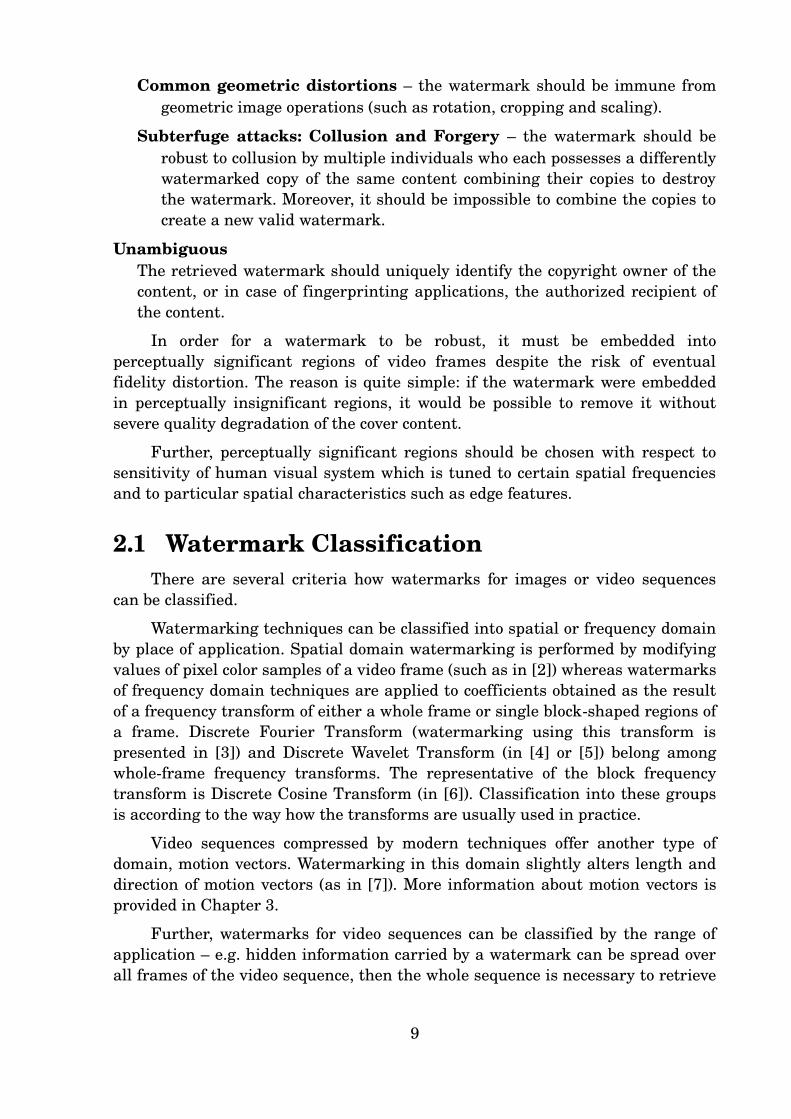
Only the pictures that go in the stream before the current slice can be used

for prediction. Thus, even following pictures in display order used for prediction

should go before the current slice. The reason is simple: decoders need those

pictures to be able to decode predicted slices on-the-fly. Let us assume that each

picture consists of a single slice, then the difference between display and stream

order is illustrated in Figure 4 and Figure 5 (prediction dependencies are

indicated by arrows).

Figure 4: Display order of pictures

Figure 5: Stream order of pictures

3.1.3 Macroblocks

A slice is a sequence of macroblocks, as depicted in Figure 3. A macroblock,

consisting of a 16×16 block of luma samples and two corresponding blocks of

chroma samples, is used as the basic processing unit. Luma samples represent

luminance of pixels while chroma samples represent chromatic components.

15

I1 B2 B3P4 B5 B6P7 B8 B9I10 P13 B11 B12

I1 B2 B3 P4 B5 B6 P7 B8 B9 I10 P13B11 B12

A 16×16 block of luma samples consists of 16 4×4 or 4 8×8 luma sub-blocks,

depending on selected frequency transform. This partitioning is also used in a

special type of intra prediction process.

Blocks of chroma samples are compounded similarly.

A macroblock can be further partitioned (subsequently halved or quartered)

for inter prediction into blocks up to size of 4×4 luma samples.

3.2 Encoding

This section describes a scheme of the H.264 encoding process of a video

sequence. The description is restricted to grey-scaled sequences only to avoid

talking about chroma blocks which are coded in the completely same way as luma

blocks.

Considering one picture of the sequence, encoders may select between intra

and inter coding for blocks of the picture. Intra coding is usually selected for

pictures just after a scene cut while inter coding for fluently following pictures.

Scene-cut pictures typically miss any statistical dependence on previous pictures,

thus there is no reason to use inter coding. Fluently following pictures can be

imagined as e.g. a static scene without any camera movement, thus such

following pictures are very similar and inter coding is the best choice.

In practice, encoders try both ways and choose the one that have better

bit-rate to distortion ratio.

Regardless which coding is selected, the encoding process is the same. The

process is depicted in Figure 6.

A picture is partitioned into 16×16 blocks of pixel color samples called

macroblocks (MB). Then, the prediction process is invoked. Intra coded

macroblocks can use intra prediction only while inter coded ones can use both

intra and inter prediction. The subtraction of original samples and predicted

samples is called prediction residual.

The intra prediction process predicts macroblock samples from edge samples

of neighbouring macroblocks within the same picture. A special type of the

process can be, in the same way, invoked on 4×4 or 8×8 sub-blocks of the

macroblock. The mode of prediction, i.e. which and how neighbouring blocks are

used, is encoded into a single number.

The inter prediction process may partition macroblocks into 2 16×8 or 8×16

or 4 8×8 blocks and 8×8 blocks can be further partitioned into 2 8×4 or 4×8 or 4

4×4 sub-blocks. For each block, the most similar block of the same size and shape

is found in the reference pictures and its samples are used as predicted samples.

The identifier of the reference picture and the relative position of corresponding

blocks are encoded into so called motion vector.

The residual is partitioned into 16 4×4 or 4 8×8 blocks, depending on chosen

16

frequency transform. The choice is made per macroblock. Further, these blocks

are transformed to remove spatial correlation inside the blocks.

Basically, the H.264 standard provides 4×4 block transform only but it has

been extended to 8×8 blocks. The transform is a very close integer approximation

to 2D-DCT transform with pretty much the same features and qualities.

Then, the transform coefficients are quantized (Q), i.e. divided by

quantization factors and rounded. This irreversible process typically discards less

important visual information while remaining a close approximation to the

original samples. After the quantization, many of the transform coefficients are

zero or have low amplitude, thus can be encoded with a small amount of data.

Figure 6: Encoding process scheme

The quantized coefficients are dequantized, inverse transformed and added

to the predicted samples to form a block of potentially reference picture.

Finally, the intra prediction modes or the motion vectors are combined with

the quantized transform coefficients and encoded using entropy coding (EC).

Entropy coding consists in representing more likely values by less amount of data

and vice versa.

The standard offers two entropy coding methods: Context-based Adaptive

Variable Length Coding (CAVLC) and Context-based Adaptive Binary Arithmetic

Coding (CABAC). CABAC is by 5-15% more effective [10] but much more

computationally expensive than CAVLC.

Entropy encoded data are enveloped together with header information as a

slice into a NAL unit.

17

DCT

DCT-1

EC

-

IntraPrediction

InterPrediction

PictureBuffer

Q

Q-1+

motion vectorPicture

MBintra prediction mode

3.3 Decoding

The decoding process is reversal process to encoding resulting in visual

video data, as depicted in Figure 7.

Incoming slices are decoded, using the same entropy coding as in the

encoding process, up to intra prediction modes or motion vectors and quantized

transform coefficients.

Macroblock by macroblock, block by block, the quantized transform

coefficients are scaled to the former range, i.e. multiplied by dequantization

factors, and transformed by inverse frequency transform. Hereby, the prediction

residual is obtained.

Figure 7: Decoding process scheme

The prediction process is invoked using the intra prediction mode in case of

intra prediction, or the motion vector in case of inter prediction. Predicted

samples are added to the residual.

Such decoded blocks and macroblocks are joined together to form the visible

picture that is stored in the buffer of reference pictures for the inter prediction

process in next pictures.

In both encoding and decoding processes, deblocking filter process is invoked

over decoded pictures to increase final visual quality. The process eliminates

blocking artefacts on block borders, as may be seen in video sequences

compressed according to many of previous video coding standards at lower

bit-rates.

18

DCT-1EC-1

IntraPrediction

InterPrediction

Q-1 +

motion vector

Picture

MB

intra prediction mode

PictureBuffer

Chapter 4

Implementation Details

This chapter deals with implementation details of the software framework

for watermark embedding and detection.

A partial decoder / encoder (codec), as mentioned in Section 2.2, of H.264

video streams has been implemented in order to obtain transform coefficients for

direct watermark embedding in frequency domain and further processing for

embedding in spatial domain.

Further, a generic framework for watermarking of H.264 streams in both

spatial and frequency domains has been designed and implemented. In this

framework, three different watermarking methods have been written. The

practical comparison of these methods is presented in Chapter 5.

4.1 The H.264 Codec

The partially decoding part of the codec is implemented according to the

H.264 standard [9]. Of course, there are free implementations of the standard but

writing an own helps to deeply understand the standard and video compression

at all. Moreover, the transform coefficients are needed only, not fully decoded

visible pictures.

The decoder produces all syntactical elements of a stream which are

relevant for watermarking. In particular, it decodes and parses SPSs, PPSs, slices

and macroblocks up to transform coefficients. During the process, it checks

whether the decoded elements and the whole stream are correct. When an error

occurs, it is reported by a message of particular severity level (critical error, error,

warning etc.) and decoding of the current NAL unit ends immediately.

The encoding part of the codec is written as an inverse process to decoding

because the standard contains only fragment information about the process. The

19

encoder is able to handle slices and macroblocks only; neither SPSs nor PPSs are

supported because the stream properties are not changed during watermark

embedding.

The codec is tested on various H.264 video sequences and even on official

tests contained in [11]. But there are still limitations which are listed in Section

4.1.2.

The codec is written in programming language C as a library. Because the

names of functions and variables follow labels from the standard and algorithms

are rewritten from the standard and only slightly optimized, the source code is

commented briefly.

Although the codec has a very limited application, the source code has over

11 000 lines.

4.1.1 Supported Features

The codec is able to decode the following features:

� SPS and PPS,

� both CAVLC and CABAC entropy coding,

� partitioning of pictures into slices,

� both frame and field slices,

� all slice types: I, P and B,

� all syntactical elements of slices: all macroblock types (i.e. partitioning), both

4×4 and 8×8 transform coefficients, intra prediction modes, motion vectors etc.

4.1.2 Known Bugs and Limitations

No bugs are known at the moment but the codec does not support the

following features:

� only syntactical elements and several derived values are decoded – no visual

data is provided,

� macroblock-adaptive frame-field coded slices, i.e. slices which contain both

frame and field macroblocks together, are not supported,

� memory management control is not considered – no reference pictures are

buffered,

� reference picture list reordering is not fully decoded and applied,

� unsupported NAL units:

� Auxiliary Coded Picture (a supplement picture mixed to the primary

picture by alpha blending),

� Sequence Parameter Set Extension (alpha blending parameters for

20

auxiliary coded pictures),

� Supplemental Enhancement Information (necessary information for

correct video playback and other data – timing information, buffer

management hints, user data, scene information, pan-scan information,

spare picture information, still frames etc.),

� Slice Data Partitions, i.e. partitions of too big slices.

4.2 The Watermarking Framework

The framework is designed for easiness when implementing any particular

watermarking method in either spatial or frequency domain of H.264 video

streams. Then, implementation of a method consists in writing only two

functions, one for watermark embedding and the other for watermark detection.

4.2.1 GStreamer Multimedia Framework

In practice, a H.264 video stream is usually enveloped (multiplexed / muxed)

together with an audio stream into a multimedia container format such as Audio

Video Interleave (AVI) or Matroska (MKV). In order to avoid implementing of

unpacking (demultiplexing / demuxing) various container formats and separating

out the video stream, the watermarking framework is implemented as a plugin in

the open source multimedia framework called GStreamer [12].

GStreamer is a library that allows the construction of graphs of

media-handling components, ranging from simple audio playback to complex

audio and video processing.

A graph, also called a pipeline, of a generic audio-video player is illustrated

in Figure 8.

Figure 8: Generic audio-video player pipeline

The file source reads the input file of particular container format and

forwards its data to the demuxer. The demuxer demultiplexes the container

format resulting in audio and video data blocks. The video decoder decodes video

data and forms pictures of the video sequence. Then, pictures are displayed by

the video sink on the screen with the correct timing to be a fluently moving video.

Audio data are decoded by the audio decoder and reproduced by the audio sink on

21

FileSource

Demuxer

VideoDecoder

AudioDecoder

ImageSink

AudioSink

InputFile

video

audio

����

loud speakers.

The watermark plugin stands for an element in a suchlike pipeline. The

plugin can be divided into two parts: the GStreamer part and the main part, and

works in either embedding (see Section 4.2.2) or detection (see Section 4.2.3)

mode.

The GStreamer part implements the GStreamer interface which is

thoroughly documented on the project's website [12], thus the source code is only

briefly commented.

This part parses incoming data blocks of H.264 stream into NAL units

which are further decoded using the codec, mentioned in Section 4.1. As soon as a

slice is decoded, it is forwarded to the main part of the plugin. Then, in

embedding mode, the watermarked slice is encoded again and sent to the output,

or in detection mode, detection statistics are given.

The main part does watermark embedding or detection, depending on the

mode.

The plugin is written as a library in programming language C and the

source code counts about 3 500 lines. The usage of the plugin is described in

Appendix B and the documentation is provided in Appendix C.

4.2.2 Embedding

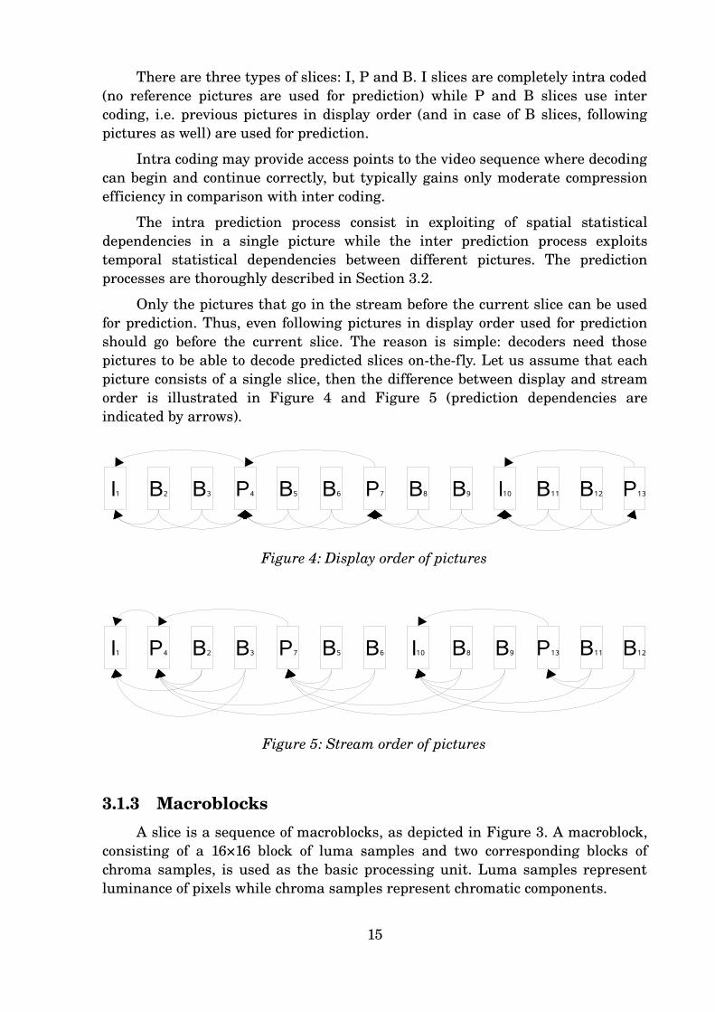
In the embedding mode, the plugin accepts a H.264 stream as the input,

invokes the embedding process and outputs the same but possibly watermarked

H.264 stream. The embedding pipeline is illustrated in Figure 9.

Figure 9: Watermark pipeline in embedding mode

Non-watermarked slices and other NAL units are passed through without

any changes.

In the current implementation of the plugin, only intra coded slices are

watermarked. This is because inter prediction is quite complicated and is not

necessary for objectiveness of the thesis results.

Inputs to the embedding process are:

22

FileSource

Watermark(embedding)

InputFile

H.264video

audio

H.264video

Demuxer MuxerFileSink

OutputFile

� an intra coded slice,

� content ID – the identifier of the cover content,

� copy ID – the identifier of particular cover content copy,

� weight – the weight factor specifying the watermark strength.

Output of this process is the watermarked slice.

At the beginning of the entire embedding process, the watermark is

generated. The watermark is a pseudo-random noise signal covering one whole

picture of the video sequence. The signal sample (i.e. watermark element) values

are each either 1 or -1.

The watermark is partitioned into blocks, as the picture is partitioned into

macroblocks, thus one block of the watermark is embedded into one macroblock of

the picture. Dimension of the blocks depends on particular watermarking

method.

The watermark is generated so that the sum of values of the watermark

block elements is zero. The reason is to equal number of 1 and -1 in blocks to

balance probability of changes caused by an attack. The pseudo-random

generator is initialized by the identifier of the cover content copy – copy ID.

Let us denote such generated watermark as pure watermark.

One block of the watermark carries one bit of hidden information. Hidden

information in this implementation is the identifier of the cover content – content

ID. Content ID is typically represented by much less bits than the number of

watermark elements, thus bits of the ID are pseudo-randomly spread over all

watermark elements where the usual binary values {0, 1} are replaced by {-1, 1}.

The pseudo-random generator is initialized by the ID itself. Another reason why

the ID is spread is that the robustness is increased hereby and the spreading

stands for a simple self error-correcting code due to redundancy.

Bits of hidden information (spread content ID) modulate the signal. When -1

is to be encoded, values of the block elements are inverted, i.e. from each 1

becomes -1 and vice versa, and when 1 is to be encoded, values of the block

elements remain unchanged. This can be expressed like this:

(5)

Here, WM is modulated watermark, WP is pure watermark, Wij is j-th element

value in i-th watermark block and Ii is i-th bit value of hidden information.

The robustness can be improved by multiplying watermark element values

by the weight factor a (the weight factor can be locally adjustable to track local

spatial characteristics, thus to dynamically balance robustness and

perceptibility):

(6)

23

W ij

M=W ij

P�I i

W ij

M=aW ij

P�I i

But the description is restricted to the former values in order to be less confusing;

proposed algorithms, processes and calculations do not change.

Figure 10 illustrates content ID spreading, watermark generation and

embedding which is described below.

Figure 10: Illustration of watermark generation and embedding

Once the watermark is generated and hidden information is encoded, the

embedding process can take place.

Blocks of each macroblock could be watermarked using formula (2) in case of

frequency domain watermarks (the transform coefficients of a block are altered to

encode one watermark element) or formula (4) in case of spatial domain

watermark (corresponding sub-block of watermark block elements is forward

transformed and added to the coefficients).

However, it not as simple as it seems. The essence of the problem consists in

intra prediction. If watermarked blocks are used for intra prediction of other

blocks, distortion caused by watermark embedding spreads into the other blocks.

If there is a sequence of predictively dependent blocks, the distortion propagates

and accumulates up into the last block of the sequence which probably causes

severe, obviously not unobtrusive, fidelity distortion. Therefore, the intra

prediction error compensation is implemented to undo the distortion.

In one block of a macroblock, the embedding process proceeds as follows (the

scheme is depicted in Figure 11). The residual is obtained using inverse

frequency transform on dequantized transform coefficients. Then, the predicted

samples of both the original and the watermarked pictures are computed. Thus,

both pictures are constructed during the process. The residual is added to

predicted samples of the original picture, clipped to allowed range and stored as a

block of the original picture. The prediction error as the difference between the

watermarked picture predicted samples and the original picture predicted

24

Watermarked PictureOriginal Picture

+

1 1 0 1 01

WeightFactor

Content ID

Pure Watermark

Modulated Watermark

Spread Content ID-1

1

1 11 1-11 1 -1 1 -1 1 1-11-1 -1

1-111 -1 1

-1-1 -11

1-1

-1 -1-1

1-1-1 -1 1 1

1

1-1-1

-11 1-1 -11-1 1 1 -1

1

1 -111 1-1 -11 1-11 -1 -1 1 -1 -1 1-1-1 -11 -11 1-1-1 1 1 -1 -1 -1 111 1-1 1-1 -11 -1 1 -1 -1 1 -1-11 -1-1 -1-1 1-1-1 1 -1 1 1 -1 11

-1

11

1

samples is subtracted from the residual.

Such compensated residual is now ready for direct watermark embedding in

the spatial domain. It depends on particular watermarking method whether the

embedding process is controlled by the residual only or by the predicted samples

as well.

Then, the residual is forward transformed and quantized. Note that the

spatial domain watermark can be impaired by the quantization.

The quantized transform coefficients may be directly watermarked in the

frequency domain.

The coefficients, watermarked either in the spatial domain or in the

frequency domain, are dequantized and inverse transformed again. Such obtained

residual is added (and clipped) to predicted samples from the watermarked

picture to form a block of the watermarked picture.

Figure 11: Watermark element embedding scheme with intra prediction

error compensation

If the samples were not clipped, the reconstruction of the pictures would not

be necessary. The error compensation would be possible by subtracting samples

that are intra predicted from the difference in the residual caused by watermark

25

DCT-1EC-1

IntraPrediction

Q-1

intra prediction mode

IntraPrediction

intra prediction mode

Watermarkembedding inspatial domain

Watermarkembedding infreq. domain

DCT

Q

EC

DCT-1Q-1

Original Picture

MB

+

--

+

Watermarked Picture

MB

embedding.

Anyway, the pictures are used for measuring distortion caused by

watermark embedding. Distortion in one picture is measured by peak

signal-to-noise ratio (PSNR) which is the most commonly measure of quality of

reconstruction in image compression:

(7)

where MAXI is the maximum pixel color sample value (usually 255) of any

picture, P is the original picture, Pi is a sample value of the original picture and

P*i is a sample value of the watermarked picture.

At the end of the entire embedding process, average PSNR over all

watermarked pictures is estimated and printed.

Distortion expressed by PSNR relates to perceptibility of the watermark.

The practical results are presented in Chapter 5.

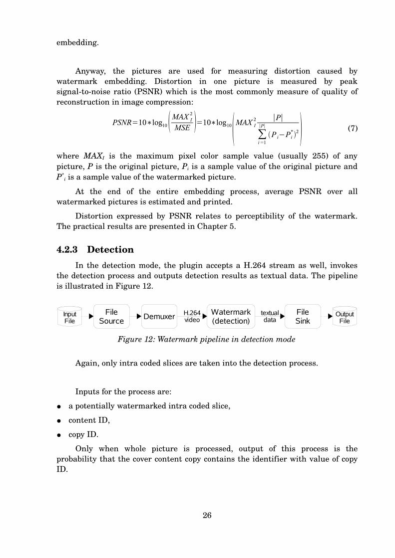
4.2.3 Detection

In the detection mode, the plugin accepts a H.264 stream as well, invokes

the detection process and outputs detection results as textual data. The pipeline

is illustrated in Figure 12.

Figure 12: Watermark pipeline in detection mode

Again, only intra coded slices are taken into the detection process.

Inputs for the process are:

� a potentially watermarked intra coded slice,

� content ID,

� copy ID.

Only when whole picture is processed, output of this process is the

probability that the cover content copy contains the identifier with value of copy

ID.

26

PSNR=10�log10 �MAX I

2

MSE �=10�log10�MAX I

2 �P�

�i=1

�P�

�P iPi*�2 �

FileSource

Watermark(detection)

InputFile

H.264video

textualdataDemuxer

FileSink

OutputFile

At the beginning of the entire process, the same pure watermark as in the

embedding process is generated. The pure watermark is further used for

correlation with the detected watermark to retrieve hidden information.

In each macroblock, watermark block element values carrying one hidden

information bit are obtained using particular watermarking method (the scheme

is depicted in Figure 13). In case of frequency domain, the transform coefficients

are directly accessible. In case of spatial domain, the coefficients have to be

dequantized and inverse transformed in order to obtain the residual. It is further

added to predicted samples and clipped giving picture samples suitable for

detection. In this case, the residual is not enough because it depends on selected

intra prediction mode which could change after an attack.

Figure 13: Watermark element detection scheme

Obtained watermark block element values are compared with the

corresponding element values of the pure watermark. When the two

corresponding values match, 1 has been encoded, while when they differ, -1 has

been encoded. Remember the modulation of pure watermark by bits of hidden

information in the embedding process: when -1 was to be encoded, values of the

watermark block elements are inverted, i.e. each 1 becomes -1 and vice versa

(thus differ), and when 1 was to be encoded, values of the block elements remain

unchanged (thus match).

But in practice, especially after an attack, the corresponding values in one

block need not 100% match or differ. Therefore, some correlation mechanism has

to be proceeded. The correlation sum for i-th watermark block is computed:

(8)

where WPij is j-th element value of the pure watermark block and W*

ij is j-th

element value of the detected watermark block.

When the block encodes 1 (corresponding values match – they are either (1,

27

C i=�j

W ij

P�W ij

*

DCT-1EC-1

IntraPrediction

Q-1 +

Picture

MB

intra prediction mode

Watermarkdetection infreq. domain

Watermarkdetection in

spatial domain

1) or (-1, -1)), the sum can get the maximum positive value, while when the block

encodes -1 (corresponding values differ – the are either (1, -1) or (-1, 1)), the sum

can get the minimum negative value. The middle value between these two

extremes is 0. Thus, when the sum is greater than 0, 1 is returned, when the sum

is lower then 0, -1 is returned, and when the sum is 0, the value can not be

determined and does not participate in the following process.

Once all macroblocks are processed and hidden information bits are

retrieved, it is time to merge the bits to form the detected content ID. The merge

is done in the reverse way to content ID spreading in the embedding process. One

content ID bit value is derived from the hidden information bits from those

macroblocks that contain the bit. The spreading determines which macroblocks

are taken. The value of the bit is the sign of the sum of the hidden information

bits. When the sum is greater than 0, the value is 1, when the sum is lower than

0, the value is -1, and when the sum is 0, the value can not be determined and

does not participate in the following probability estimation.

Figure 14 illustrates watermark detection and content ID merging.

Figure 14: Illustration of watermark detection

The probability of the detection success is expressed by the correlation

between the detected content ID and the input content ID. The correlation is

computed using formula (8) where watermark values are substituted by ID

values. The result is scaled to amplitude with value of 1. Then, when the

correlation coefficient is 1, the IDs 100% match and the detection is absolutely

successful, when it is -1, the IDs 100% differs, i.e. the detected ID is inverse to

input ID, thus the detection is considered successful as well. The correlation

coefficient equal to 0 means that the IDs are independent and the detection is

considered unsuccessful. The closer the coefficient is to 0 the more independent

the IDs are.

Per-picture correlation coefficients are continuously written to the output

28

Watermarked Picture

1 1 0 1 01Content ID

Pure Watermark

Spread Content ID-1

1

1 11 1-11 1 -1 1 -1 1 1-11-1 -1

1-111 -1 1

-1-1 -11

1-1

-1 -1-1

1-1-1 -1 1 1

1

1-1-1

-11 1-1 -11-1 1 1 -1

1

1 -111 1-1 -11 1-11 -1 -1 1 -1 -1 1-1-1 -11 -11 1-1-1 1 1 -1 -1 -1 111 1-1 1-1 -11 -1 1 -1 -1 1 -1-11 -1-1 -1-1 1-1-1 1 -1 1 1 -1 11

-1

1-1

1

file in order to provide detailed results for deeper analysis.

At the end of the entire detection process, average probability as average

value of absolute correlation coefficient values over all intra coded pictures is

estimated and printed. The probability expresses the detection success rate.

4.2.4 Notes

The generation of the watermark is based on spread spectrum technique

presented by Hartung [2]. Spread-spectrum watermarks are described in detail

in Section 4.3.1.

The watermark is embedded into luma samples only because human visual

system is more sensitive to changes in luminance than to chromatic components,

thus the watermark is harder to remove without severe quality degradation of

the cover content. Moreover, the chromatic channels of the video stream may be

completely removed and the video remains in former quality; the only difference

is that the video lacks colors.

To increase the watermark robustness, a different pseudo-random signal

can be generated for each picture in the embedding process. But then, a

synchronization mechanism must be implemented in the detection process to be

able to detect the watermark even if the order of the pictures is changed (or some

are missing or extra) by an attack. This is not trivial and is not implemented in

the plugin.

The generation of the pseudo-random signal is initialized by copy ID and

hidden information is created from content ID intentionally. If a cover content

copy contains more watermarks, they are represented by independent

pseudo-random signals, thus it is possible to detect each of them. If the pure

watermark were generated from content ID and hidden information from copy

ID, the advantage would be that the detection result would be just the copy ID

but copy IDs in multiple embedded watermarks would overwrite each other.

There is a weakness in the implementation because all macroblocks are

watermarked. Especially uniform areas in a picture are encoded by almost none

residual. Then, if such area is watermarked, the residual contains the watermark

alone, thus the watermark may be completely removed. The solution could be to

watermark only non-zero coefficients of residual with prejudice to robustness.

Another problem relates to watermarking of every macroblock. Because of

many coefficients that have been zero are altered to non-zero value, the bit-rate is

pretty much increased. We will see in Chapter 5 how high the increase is.

With respect to human visual system which is very sensitive to changes in

uniform areas, watermarking could be further improved to embed the watermark

only into edge features or textured areas. But the goal of the thesis is to compare

watermarking methods as they are, therefore no such extensions are

implemented.

29

4.3 Watermarking Methods

Three different watermarking methods have been implemented. One stands

for a spatial domain watermarking technique and the other two represent

frequency domain techniques.

Each method is implemented in only two functions; one is for embedding

into macroblock blocks and the other is for detection. The rest of necessary

actions does the watermarking framework.

4.3.1 Pseudo-random Noise Watermark

Pseudo-random noise watermark is inspired by spread-spectrum

communication schemes which transmit a narrow-band signal (the watermark)

via a wide-band channel (the video sequence) by frequency spreading. This

technique was presented by Hartung for uncompressed and MPEG-2 compressed

video [2]. In this thesis, it has been implemented for H.264 video streams.

This method belongs to spatial domain techniques, thus the watermark can

be impaired during the embedding process by quantization. This is compensated

by the technique itself because spread spectrum provides the reliable detection

even if the embedded watermark is impaired because of the interference from the

video sequence itself and noise arising from subsequent processing or attacks.

Nevertheless, a spread spectrum watermark is vulnerable to

synchronization error which occurs when the watermarked sequence undergoes

geometric manipulations such as scaling, cropping and rotation.

Furthermore, Stone [13] shows that advanced collusion attacks against

spread-spectrum watermarks can be successful with only one to two dozen

differently watermarked copies of the same content.

When using this method, the watermark plugin generates the pure

watermark blocks with dimension of 16. Macroblocks have the same dimension,

thus one watermark element is to be embedded into one pixel of the picture.

The embedding function is called for each block of each macroblock;

dimension of the blocks depends on selected frequency transform. The modulated

watermark is embedded as it is by simple addition to the residual, thus up to

picture samples:

(9)

The detection function is called for each block of each macroblock as well.

The detection process is based on the fact that the pseudo-random signal and the

picture are statistically independent while the signal is autocorrelated. This

method does not provide detected watermark element values to the framework

but uses the correlation sum calculation (see formula (8) above) in the framework

30

Pij*=Pij�W ij

M=P ij�aW ij

P�I i

as a part of the whole process. Then substituting detected watermark element

values by picture sample values, the evolution of the correlation sum is:

(10)

where A and B stand for contributions to the sum from the picture and from the

watermark. Let us assume that A is zero because of independence of the

pseudo-random signal and the picture, then:

(11)

In practice, A is not exactly zero, thus an error is included. The decision

process in the framework is invoked – when Ci is greater than 0, the value of the

detected hidden information bit is 1, and when Ci is lower than 0, the value is -1.

Ii is either -1 or 1 and a is greater than 0, therefore the sign of Ii sets the sign of

Ci and the detected hidden information bit is determined correctly. The greater

the weight factor a is the greater the tolerance to the error of A is provided.

The probability of detection success may be increased by applying a

high-pass filter to the sequence before the detection process in order to filter out

the host signal and keep the watermark signal alone.

4.3.2 Block Watermark

Block watermarking method belongs to frequency domain techniques. The

method consists in coding one watermark element into one block of a macroblock

residual.

Only 4×4 blocks are supported because of the following. The partitioning of

macroblock residuals into blocks may change when the video sequence undergoes

any video signal processing operation. The simplest example is recompression

with different parameters.

The problem occurs when the watermark element has been embedded into a

macroblock partitioned into 16 4×4 blocks and the partitioning has changed to 4

8×8 blocks, or vice versa. Changes made by watermark embedding in one

partitioning are basically undetectable in the other partitioning because the

transforms are not equivalent in terms of transform coefficient values. It would

be possible to convert the blocks to the former partitioning before detection but it

is not obvious which partitioning is the former one.

Therefore, the conversion to one type of partitioning has to be applied before

embedding. After embedding, the partitioning is converted back to the former

type in order to preserve macroblock properties. In the detection process, the

conversion to the same type as in the embedding process is applied before

31

C i=A�Ba �j=1

16�16

�W ij

P�2�I i=a�16�16�I i

C i=�j=1

16�16

W ij

P�Pij*=�

j=1

16�16

W ij

P��P ij�aW ij

P�I i�=�j=1

16�16

W ij

P�Pij�A

�a �j=1

16�16

�W ij

P�2�I i�B

detection.

Conversion into 8×8 blocks is out of the question because of intra prediction.

The intra prediction process for a 4×4 sub-block within one 8×8 block uses the

other 4×4 sub-blocks within that 8×8 block. Therefore, when the 8×8 block is

watermarked, the error caused by watermark embedding should be compensated

in the 4×4 sub-blocks when using the other 4×4 sub-blocks for prediction. But the

compensation may severely impair the already embedded watermark...

There is only conversion into 4×4 blocks left. In this case, intra prediction

does not give trouble. The conversion is performed by decoding (i.e. dequantizing

and inverse transforming) a 8×8 block, partitioning into 4×4 blocks and encoding

(i.e. forward transforming and quantizing) the blocks in order to obtain transform

coefficients for watermark embedding. This works pretty well but the

quantization causes visible blocking artefacts.

With respect to the reasons above, no conversion is applied and only 4×4

blocks are taken for watermark embedding. 4×4 blocks have been chosen because

4×4 block transform is more usual than 8×8 transform. Video sequences given to

both embedding and detection can be converted to required format beforehand at

the cost of eventual quality degradation.

The pure watermark blocks are generated with dimension of 4 to cover 16

4×4 macroblock blocks.

Embedding into one block proceeds as follows. Only the half of transform

coefficients that represent higher frequencies are taken. Although higher

frequencies are more vulnerable to eventual attacks, human visual system is

more sensitive to distortion in lower frequencies and modification of low

frequency coefficients causes obtrusive blocking artefacts.

When 1 (the weight factor a in fact) is to be embedded, the coefficient with

the greatest absolute value is chosen. The coefficient modification keeps the sign

of the coefficient but eventually increases its absolute value to required

robustness level. If the coefficient is positive but lower than a, the coefficient is

increased to a. If the coefficient is negative but greater than -a, the coefficient is

decreased to -a. The coefficient is remained unchanged if it is greater than a in

absolute value. If the coefficient is 0, a or -a is randomly assigned. The purpose

why all this is done is to enforce a non-zero value in the half while producing to

the lowest distortion.

When -1 is to be embedded, all coefficients in the half are set to zero. This

causes loss in detail.

Detected watermark element values are obtained directly from transform

coefficients. If all transform coefficient values in the half are zero, -1 is returned,

otherwise (if there is at least one non-zero coefficient) 1 is returned.

Recompression at lower bit-rate causes more loss in detail, thus zero

32

coefficients are hardly set to non-zero values. On the other hand, the coefficients

set to the weight factor a in absolute value can be zeroed. Therefore, a should be

set to such a high value to remain non-zero even if the video sequence undergoes

an attack.

Considering multiple embedding attack, this method is quite vulnerable

because the watermark elements are directly embedded and thus multiple

embedded watermarks overwrite each other.

The watermark can be completely destroyed by zeroing the coefficients in

the half in all macroblocks but it results in visible blocking artefacts.

4.3.3 Coefficient Watermark

Coefficient watermarking method belongs to frequency domain techniques

as well. The method consists in coding one watermark element into one transform

coefficient of a macroblock residual block.

Again, only 4×4 blocks are supported because of the same reasons as in

block watermarking method and the pure watermark block has dimension of 4.

The transform coefficient where a watermark element is to be embedded

into is pseudo-randomly chosen from the half of coefficients which represent

higher frequencies. The pseudo-random generator is initialized for each picture

by both content ID and user ID in order to increase robustness against multiple

watermark embedding and collusion attacks.

The value of the coefficient is altered in the same way as in block

watermarking method, i.e. when 1 is to be embedded, the value is eventually

increased to the weight factor a in absolute value, and when -1 is to be embedded,

the coefficient is set to zero.

In the detection process, the transform coefficient is pseudo-randomly

chosen in the same way as in the embedding process. If the coefficient is zero, -1

is returned, otherwise 1 is returned.

This method should have similar robustness qualities to block watermark

method but distortion caused by watermark embedding should be lower because

only one coefficient is altered in a block.

33

Chapter 5

Testing

Proposed watermarking methods have been exposed to several tests in order

to check up and compare their qualities and robustness. The test results are

summarized in this chapter.

The test environment consists of single test scripts written as Unix shell

scripts. If recompression is applied, a free H.264 encoder, x264 [14], is used; it is

released under the terms of the GPL license. Video signal processing tests use

video filters of MPlayer movie player [15] which is available under the GPL

licence as well.

The test scripts have been executed on several video sequences with

different characteristics. Most of them have been downloaded from

high-definition video gallery [16] on the Apple website. All the sequences have

been remuxed to Matroska [17] container format because of easiness of use (there

are both the demuxer and the muxer in the GStreamer plugin library). The list of

the sequences follows:

Elephants Dream (ED) represents an animated movie. This particular one has

been made entirely with open source graphics software, Blender. It has been

downloaded from the project's website [18].

Full Bloom (FB) is a sample of 1080p high-definition video.

Kingdom of Heaven (KH) is a trailer of the movie with the same name. The

main feature is frequent scene cuts.

Peaceful Warrior (PW) stands for a low-resolution sample.

Renaissance (R) is mostly black-and-white sequence with only a few other hues.

The Simpsons Movie (SM) is the representative of cartoon movies.

Wildlife (W) brings real images from nature with minimum camera movement.

34

Table 1 outlines characteristics of the sequences.

Table 1: Characteristics of testing video sequences

Each test script embeds a watermark into each testing video sequence using

each proposed watermarking method – block, coefficient or noise – with weight

factor from 1 to 5, applies the test itself and obtains the result.

Watermarks are generated with content ID assigned to the sequences

subsequently from 1 to 7. If not mentioned otherwise, copy ID is set to 1.

Other scripts are provided to make embedding and detection easier. These

scripts contain corresponding GStreamer pipelines. The usage is described in

Appendix B.

In the test result tables (see below), the results belonging to one method are

grouped into one column set headed by the method name where one column

contains results of the test using the weight factor given in the column header.

Row sets represent results for single testing video sequences – ED, FB, KH,

PW, R, SM and W. Rows of the sets vary depending on eventual additional test

parameter.

5.1 Perceptibility

Perceptibility expresses amount of distortion caused by watermark

embedding. In other words, it indicates how visible the watermark is. It is

measured by peak signal-to-noise ratio (PSNR) which is mentioned in Section

4.2.2. The less the value of PSNR is the more perceptible the watermark is. We

can see in the first row set of Table 2 that the perceptibility grows up with

increasing weight factor. It is obvious that block method is the most perceptible

method because of the way of embedding.

The second row set of the table contains probabilities of watermark

detection success in non-attacked sequences as given by the detector. Note lower

probabilities when using noise method with low weight factors caused by the

interference from the video sequences and quantization.

35

Resolution # I Frames Description

ED 10:54 24.000 1667.29 31.34 638 animatedFB 01:41 23.976 8228.74 101.28 102 HD in full resolutionKH 02:40 23.976 2528.07 34.54 105 frequent scene cutsPW 02:20 29.970 239.36 3.87 67 low resolutionR 01:18 23.976 1701.18 17.02 71 black-and-white

SM 02:17 23.976 2103.66 39.29 97 cartoonW 02:20 29.970 2015.86 45.06 14 nature

Length [min:s]

Frame-rate [frames/s]

�Bit rate [kb/s]

Av. I Frame Size [kB]

720×4051920×1080852×360320×136848×480848×352960×540

Table 2: Perceptibility test results. Probabilities of detection success in non-attacked sequences and

bit-rate growth ratios in addition.

Block Coefficient Noise1 2 3 4 5 1 2 3 4 5 1 2 3 4 5

PS

NR

[dB

]

ED 41.92 38.79 36.23 34.13 32.42 44.16 39.72 36.63 34.27 32.42 49.21 39.75 36.69 34.75 33.23FB 43.56 38.40 35.09 32.67 30.78 43.59 38.33 35.01 32.58 30.69 53.71 39.91 36.32 34.41 32.98KH 44.54 41.46 38.80 36.65 34.89 46.53 42.08 38.93 36.56 34.72 47.43 40.04 37.12 35.11 33.51PW 40.63 37.14 34.41 32.19 30.43 42.47 37.80 34.65 32.25 30.40 54.21 40.52 36.54 34.31 32.84R 44.21 40.02 37.09 34.62 32.79 45.02 40.14 36.98 34.48 32.61 49.81 40.33 36.96 34.77 33.19

SM 35.63 34.15 32.59 31.10 29.74 40.98 37.34 34.46 32.19 30.37 53.35 40.37 36.49 34.39 32.90W 40.25 36.03 32.95 30.59 28.72 41.10 36.06 32.78 30.37 28.49 61.14 40.48 36.12 33.84 32.46

Pro

babili

ty

ED 1.00 1.00 1.00 1.00 1.00 1.00 1.00 1.00 1.00 1.00 0.87 1.00 1.00 1.00 1.00FB 1.00 1.00 1.00 1.00 1.00 1.00 1.00 1.00 1.00 1.00 0.88 1.00 1.00 1.00 1.00KH 1.00 1.00 1.00 1.00 1.00 1.00 1.00 1.00 1.00 1.00 0.92 1.00 1.00 1.00 1.00PW 1.00 1.00 1.00 1.00 1.00 1.00 1.00 1.00 1.00 1.00 0.46 0.92 0.99 1.00 1.00R 1.00 1.00 1.00 1.00 1.00 1.00 1.00 1.00 1.00 1.00 0.89 0.99 1.00 1.00 1.00

SM 1.00 1.00 1.00 1.00 1.00 1.00 1.00 1.00 1.00 1.00 0.80 0.99 1.00 1.00 1.00W 1.00 1.00 1.00 1.00 1.00 1.00 1.00 1.00 1.00 1.00 0.37 1.00 1.00 1.00 1.00ED 104% 107% 109% 111% 112% 106% 109% 111% 113% 115% 104% 116% 124% 130% 135%FB 109% 114% 116% 119% 121% 110% 115% 117% 120% 123% 102% 118% 131% 141% 150%KH 102% 104% 104% 105% 106% 103% 104% 105% 106% 107% 104% 110% 114% 117% 119%PW 103% 104% 105% 106% 107% 103% 105% 106% 107% 108% 102% 107% 111% 114% 117%R 109% 113% 115% 117% 119% 110% 115% 117% 119% 121% 109% 126% 138% 146% 152%

SM 102% 104% 105% 106% 107% 103% 105% 106% 107% 108% 101% 107% 112% 115% 118%W 101% 101% 101% 102% 102% 101% 101% 102% 102% 102% 100% 101% 102% 103% 104%ED 128% 148% 158% 172% 182% 138% 160% 172% 187% 198% 125% 204% 261% 303% 332%FB 190% 237% 260% 287% 309% 196% 246% 272% 301% 325% 120% 278% 411% 509% 590%KH 131% 150% 160% 174% 183% 139% 160% 172% 187% 198% 158% 240% 296% 334% 363%PW 144% 170% 183% 199% 211% 155% 183% 198% 216% 230% 126% 208% 277% 329% 367%R 221% 276% 303% 333% 358% 233% 296% 327% 360% 388% 227% 453% 605% 714% 793%

SM 122% 137% 144% 153% 160% 132% 149% 158% 168% 175% 111% 164% 207% 239% 263%W 142% 168% 181% 199% 212% 150% 178% 194% 214% 229% 102% 157% 220% 271% 310%

Bit-r

ate

Ratio

ove

r A

ll S

lices

Bit-r

ate

Ratio

ove

r I S

lices

The third and the fourth row sets contain the bit-rate growth ratio in

percent to the former bit-rate over either all slices or I slices only. Block method

increases bit-rate less in comparison with coefficient method because when 0 is

embedded, a half of transform coefficients are zeroed in block method while only

one coefficient is zeroed in coefficient method. Anyway, bit-rate is increased the

most when using noise method. This is mostly obvious in Renaissance because of

many uniform areas which are represented by small amount of data in the former

compressed video stream.

Each test iteration has been executed with five different copy IDs; values in

the table are average values of corresponding five results.

Figure 15 and Figure 16 show the difference between the original picture

and the watermarked one using noise method with weight factor of 20 for

demonstration.

Figure 15: Original picture Figure 16: Watermarked picture

Because of inter coded pictures may use watermarked pictures as reference

pictures in inter prediction, distortion caused by watermark embedding

propagates, as visible in Figure 17 and Figure 18. Therefore, the inter prediction

compensation is to be implemented in future work.

Figure 17: Original inter coded picture Figure 18: Distorted inter coded picture

In practice, weight factor of 2 is a good compromise between robustness and

perceptibility.

37

5.2 Uniqueness

Uniqueness of the watermark means that the detector should return

significantly higher probability in case of copy ID which has been embedded than

in case of other copy IDs.

In each iteration, the test tries 100 different copy IDs including the correct

one – it is 10 for weight factor of 1, 30 for weight factor of 2 etc.

The results are illustrated in the following charts. The horizontal axes

represent the 100 different copy IDs and the vertical axes stand for the detector

responses.

Although probabilities achieve lower values when using noise method with

low weight factors, this method gives the highest distance of the correct copy ID

probability from the other values and the narrowest spread of the other values.

10 30 50 70 90

0

0.1

0.2

0.3

0.4

0.5

0.6

0.7

0.8

0.9

1

Block - Elephants Dream

1

2

3

4

5

10 30 50 70 90

0

0.1

0.2

0.3

0.4

0.5

0.6

0.7

0.8

0.9

1

Block - Full Bloom

1

2

3

4

5

10 30 50 70 90

0

0.1

0.2

0.3

0.4

0.5

0.6

0.7

0.8

0.9

1

Block - Kingdom of Heaven

1

2

3

4

5

10 30 50 70 90

0

0.1

0.2

0.3

0.4

0.5

0.6

0.7

0.8

0.9

1

Coefficient - Elephants Dream

1

2

3

4

5

10 30 50 70 90

0

0.1

0.2

0.3

0.4

0.5

0.6

0.7

0.8

0.9

1

Coefficient - Full Bloom

1

2

3

4

5

10 30 50 70 90

0

0.1

0.2

0.3

0.4

0.5

0.6

0.7

0.8

0.9

1

Coefficient - Kingdom of Heaven

1

2

3

4

5

10 30 50 70 90

0

0.1

0.2

0.3

0.4

0.5

0.6

0.7

0.8

0.9

1

Noise - Elephants Dream

1

2

3

4

5

10 30 50 70 90

0

0.1

0.2

0.3

0.4

0.5

0.6

0.7

0.8

0.9

1

Noise - Full Bloom

1

2

3

4

5

10 30 50 70 90

0

0.1

0.2

0.3

0.4

0.5

0.6

0.7

0.8

0.9

1

Noise - Kingdom of Heaven

1

2

3

4

5

38

10 30 50 70 90

0

0.1

0.2

0.3

0.4

0.5

0.6

0.7

0.8

0.9

1

Block - Peaceful Warrior

1

2

3

4

5

10 30 50 70 90

0

0.1

0.2

0.3

0.4

0.5

0.6

0.7

0.8

0.9

1

Block - Renaissance

1

2

3

4

5

10 30 50 70 90

0

0.1

0.2

0.3

0.4

0.5

0.6

0.7

0.8

0.9

1

Block - The Simpsons Movie

1

2

3

4

5

10 30 50 70 90

0

0.1

0.2

0.3

0.4

0.5

0.6

0.7

0.8

0.9

1

Block - Wildlife

1

2

3

4

5

10 30 50 70 90

0

0.1

0.2

0.3

0.4

0.5

0.6

0.7

0.8

0.9

1

Coefficient - Peaceful Warrior

1

2

3

4

5

10 30 50 70 90

0

0.1

0.2

0.3

0.4

0.5

0.6

0.7

0.8

0.9

1

Coefficient - Renaissance

1

2

3

4

5

10 30 50 70 90

0

0.1

0.2

0.3

0.4

0.5

0.6

0.7

0.8

0.9

1

Coefficient - The Simpsons Movie

1

2

3

4

5

10 30 50 70 90

0

0.1

0.2

0.3

0.4

0.5

0.6

0.7

0.8

0.9

1

Coefficient - Wildlife

1

2

3

4

5

10 30 50 70 90

0

0.1

0.2

0.3

0.4

0.5

0.6

0.7

0.8

0.9

1

Noise - Peaceful Warrior

1

2

3

4

5

10 30 50 70 90

0

0.1

0.2

0.3

0.4

0.5

0.6

0.7

0.8

0.9

1

Noise - Renaissance

1

2

3

4

5

10 30 50 70 90

0

0.1

0.2

0.3

0.4

0.5

0.6

0.7

0.8

0.9

1

Noise - The Simpsons Movie

1

2

3

4

5

10 30 50 70 90

0

0.1

0.2

0.3

0.4

0.5

0.6

0.7

0.8

0.9

1

Noise - Wildlife

1

2

3

4

5

Using block method, we cannot consider the detection to be successful if the

detector returns value below 0.6. Using coefficient method, the threshold limit is

0.5, and it is below 0.4 in case of noise method. Note that the spread, thus the

threshold limit as well, depends on particular video sequence.

39

5.3 Time Consumption

This section discusses time consumption of both the embedding and the

detection pipelines. The time has been measured by standard Unix utility called

time; the user-space time has been considered only. Average results of three

iterations in Table 3 show that all the methods are basically equivalent in

embedding but noise method is the worst in detection because of visual data

decoding.

The test has been executed on a machine with the following configuration:

� Intel Pentium M (Centrino) processor, 1.60GHz, 3200 bogomips

� 512MB DDR PC2700 memory, 333MHz

� openSUSE 10.1 operating system

Table 3: Time consumption test results

The test has proved that the plugin is applicable in practice.

5.4 Robustness

Robustness test scripts simulate real attacks applied either intentionally or

unintentionally to watermarked video sequences. In the simulations, they have

been executed on pre-filtered watermarked sequences – the sequences have been

remuxed in order to contain (besides parameter sets) intra coded slices only

because the watermark is embedded into intra coded slices only.

Most of the tests proceeds as follows.

A watermarked pre-filtered sequence is converted using MPlayer to the raw

video stream of single images, one image per frame. During the conversion, the

video signal processing filter is applied eventually.

Then, the raw stream is compressed by x264 encoder producing H.264 video

stream at the former bit-rate with intra coded slices only, and muxed to the

Matroska container format.

The recompression at the former bit-rate obviously impairs the embedded

watermark but the attacks are simulated more faithfully. The impairment rate of

recompression is measured in Section 5.4.1.

Finally, the detection process takes place in such an attacked sequence. The

40

Resolution # I FramesEmbedding Time [s] Detection Time [s]

Block Coeff. Noise Block Coeff. NoiseED 720×405 638 48.52 49.85 48.22 16.11 17.66 23.38FB 1920×1080 102 43.77 44.45 44.08 14.83 16.43 25.44KH 852×360 105 9.18 9.38 9.90 2.98 3.24 4.65PW 320×136 67 2.03 2.07 2.09 0.35 0.37 0.53R 848×480 71 6.25 6.38 6.78 2.03 2.25 3.59

SM 848×352 97 8.25 8.52 8.51 2.80 3.02 4.26W 960×540 14 3.21 3.25 3.92 0.77 0.82 1.84

probabilities of watermark detection success given by the detector are

summarized in tables in the following sections.

5.4.1 Recompression

This test uses MPlayer with no filter applied. Recompression is applied at

four different bit-rates – at the former bit-rate (100%) and at 75%, 50% and 25%

of the former bit-rate. The results are summarized in Table 4 where the bit-rate

ratios are listed in column named BR.

Table 4: Recompression test results

All three methods are robust at similar level. Watermarks from all video

sequences have been successfully detected after recompression at up to 50% of the

former bit-rate; from some sequences even after recompression at 25% of the

former bit-rate. Only the recompression of Wildlife using noise method with

weight factor of 1 can be considered to be a successful attack. The watermark is

impaired the most in Renaissance because of the greatest bit-rate growth during

watermark embedding.

Note that the watermark quite resists to recompression at the former

bit-rate, thus the results of the other tests using recompression are distorted only

a bit.

41

Block Coefficient NoiseBR 1 2 3 4 5 1 2 3 4 5 1 2 3 4 5

ED

100% 1.00 1.00 1.00 1.00 1.00 1.00 1.00 1.00 1.00 1.00 0.79 0.98 1.00 1.00 1.0075% 0.99 0.99 1.00 1.00 1.00 0.98 0.99 1.00 1.00 1.00 0.67 0.97 1.00 1.00 1.0050% 0.92 0.95 0.96 0.96 0.97 0.84 0.96 0.98 0.97 0.98 0.44 0.91 0.98 1.00 1.0025% 0.71 0.73 0.77 0.76 0.78 0.37 0.56 0.76 0.81 0.83 0.22 0.60 0.80 0.89 0.94

FB

100% 1.00 1.00 1.00 1.00 1.00 1.00 1.00 1.00 1.00 1.00 0.75 1.00 1.00 1.00 1.0075% 0.98 0.98 0.97 0.94 0.92 1.00 1.00 1.00 0.99 0.99 0.67 1.00 1.00 1.00 1.0050% 0.92 0.94 0.91 0.91 0.87 1.00 0.99 0.99 0.97 0.98 0.51 1.00 1.00 1.00 1.0025% 0.42 0.75 0.77 0.74 0.72 0.28 0.88 0.88 0.88 0.84 0.28 0.93 0.99 1.00 0.99

KH

100% 0.99 1.00 1.00 1.00 1.00 0.97 1.00 1.00 1.00 1.00 0.84 1.00 1.00 1.00 1.0075% 0.95 0.97 0.97 0.99 1.00 0.91 0.95 0.97 0.98 1.00 0.71 0.99 1.00 1.00 1.0050% 0.90 0.89 0.91 0.91 0.93 0.78 0.87 0.90 0.90 0.91 0.50 0.91 0.98 1.00 1.0025% 0.70 0.70 0.71 0.71 0.72 0.38 0.50 0.62 0.68 0.72 0.30 0.67 0.79 0.87 0.91

PW

100% 0.86 0.98 0.99 1.00 1.00 0.83 0.96 0.99 0.99 1.00 0.31 0.77 0.89 0.96 0.9975% 0.68 0.79 0.90 0.91 0.97 0.62 0.77 0.87 0.91 0.95 0.13 0.52 0.74 0.87 0.9350% 0.50 0.59 0.67 0.68 0.70 0.33 0.55 0.66 0.68 0.71 0.09 0.26 0.49 0.61 0.7225% 0.23 0.24 0.27 0.31 0.36 0.08 0.12 0.24 0.28 0.33 0.10 0.12 0.19 0.26 0.33

R

100% 0.80 0.79 0.81 0.82 0.85 0.75 0.76 0.80 0.78 0.79 0.46 0.88 0.96 0.98 1.0075% 0.71 0.69 0.70 0.71 0.72 0.63 0.62 0.66 0.66 0.69 0.30 0.69 0.86 0.94 0.9650% 0.55 0.59 0.59 0.60 0.59 0.44 0.49 0.50 0.53 0.53 0.22 0.51 0.64 0.71 0.7825% 0.27 0.25 0.23 0.23 0.24 0.10 0.13 0.15 0.19 0.19 0.11 0.20 0.30 0.39 0.48

SM

100% 1.00 1.00 1.00 1.00 1.00 1.00 1.00 1.00 1.00 1.00 0.44 0.88 0.99 1.00 1.0075% 1.00 1.00 1.00 1.00 1.00 0.98 0.99 1.00 1.00 1.00 0.24 0.69 0.94 0.98 1.0050% 0.98 0.99 0.98 0.98 0.98 0.93 0.96 0.98 0.98 0.98 0.18 0.53 0.80 0.90 0.9525% 0.93 0.92 0.93 0.94 0.93 0.63 0.65 0.73 0.76 0.81 0.15 0.29 0.49 0.63 0.72

W

100% 0.99 1.00 1.00 1.00 1.00 0.99 1.00 1.00 1.00 1.00 0.23 0.95 1.00 1.00 1.0075% 0.85 1.00 1.00 0.99 1.00 0.86 1.00 1.00 1.00 1.00 0.15 0.87 0.99 0.98 1.0050% 0.78 0.77 0.83 0.95 1.00 0.62 0.70 0.92 0.98 1.00 0.17 0.70 0.90 0.96 0.9725% 0.45 0.33 0.35 0.37 0.46 0.22 0.31 0.33 0.40 0.48 0.09 0.49 0.75 0.87 0.92

5.4.2 Scaling

The scaling test scales down the watermarked video sequences to the

specified resolution using MPlayer bicubic “scale” filter. The resolution is given by

scaling factor (column in Table 5 named SF) which determines how much the

images of the output raw stream are scaled down – e.g. scaling factor of 1/4

means that the image area size is reduced 4-times, i.e. both width and height are

halved.

The raw stream is compressed at the scaling factor fragment of the former

bit-rate, i.e. for example scaling factor of 1/4 means 1/4 of the former bit-rate.

Then, the compressed stream is scaled up back to the former resolution and

recompressed at the former bit-rate because the synchronization of the pure

watermark with the tested video sequence in the detection process is out of scope

of this thesis. Moreover, the human operator which would convert the sequence to

the former stadium is better than any artificial intelligence automaton.

Table 5: Scaling test results

Looking at the results, we can say that noise method is more robust than the

other two methods, especially for lower scaling factors. Anyway, the higher

resolution the sequence has the less impaired the watermark is.

42

Block Coefficient NoiseSF 1 2 3 4 5 1 2 3 4 5 1 2 3 4 5

ED

1/2 0.34 0.64 0.90 0.97 0.99 0.15 0.30 0.59 0.78 0.88 0.28 0.81 0.96 0.99 1.00 1/3 0.19 0.23 0.39 0.59 0.76 0.12 0.14 0.17 0.24 0.34 0.21 0.62 0.87 0.96 0.99 1/4 0.15 0.15 0.17 0.23 0.34 0.12 0.13 0.13 0.15 0.17 0.18 0.49 0.73 0.87 0.95 1/5 0.14 0.14 0.14 0.16 0.17 0.12 0.13 0.14 0.13 0.13 0.16 0.42 0.62 0.78 0.88

FB

1/2 0.44 0.98 1.00 1.00 1.00 0.27 0.80 0.97 1.00 1.00 0.33 0.98 1.00 1.00 1.00 1/3 0.21 0.52 0.92 0.99 1.00 0.13 0.24 0.59 0.82 0.93 0.27 0.90 0.99 1.00 1.00 1/4 0.14 0.13 0.15 0.18 0.20 0.11 0.13 0.15 0.14 0.14 0.24 0.82 0.97 1.00 1.00 1/5 0.13 0.16 0.21 0.31 0.45 0.12 0.13 0.14 0.18 0.22 0.21 0.74 0.93 0.98 1.00

KH

1/2 0.42 0.65 0.82 0.90 0.94 0.15 0.30 0.46 0.63 0.75 0.39 0.85 0.98 1.00 1.00 1/3 0.22 0.35 0.49 0.59 0.70 0.12 0.16 0.18 0.26 0.31 0.32 0.71 0.88 0.96 0.99 1/4 0.15 0.15 0.16 0.17 0.17 0.13 0.13 0.12 0.13 0.12 0.28 0.59 0.77 0.88 0.94 1/5 0.16 0.15 0.17 0.19 0.22 0.12 0.12 0.13 0.14 0.14 0.26 0.55 0.71 0.81 0.88

PW

1/2 0.13 0.21 0.41 0.60 0.71 0.08 0.09 0.15 0.23 0.31 0.12 0.26 0.41 0.58 0.70 1/3 0.08 0.11 0.14 0.17 0.26 0.08 0.09 0.09 0.09 0.10 0.12 0.19 0.30 0.42 0.51 1/4 0.11 0.10 0.09 0.09 0.11 0.08 0.10 0.08 0.09 0.09 0.12 0.15 0.23 0.31 0.34 1/5 0.08 0.10 0.10 0.10 0.10 0.08 0.09 0.08 0.09 0.09 0.11 0.17 0.22 0.27 0.30

R

1/2 0.20 0.41 0.51 0.65 0.69 0.11 0.23 0.33 0.43 0.50 0.29 0.56 0.70 0.79 0.86 1/3 0.13 0.19 0.30 0.41 0.48 0.10 0.10 0.14 0.20 0.24 0.21 0.42 0.57 0.66 0.72 1/4 0.09 0.09 0.09 0.09 0.12 0.10 0.08 0.09 0.09 0.07 0.14 0.28 0.39 0.49 0.56 1/5 0.08 0.11 0.10 0.10 0.14 0.10 0.08 0.09 0.11 0.09 0.16 0.24 0.35 0.46 0.53

SM

1/2 0.33 0.49 0.70 0.83 0.92 0.15 0.21 0.32 0.47 0.61 0.19 0.44 0.67 0.82 0.92 1/3 0.19 0.24 0.31 0.42 0.52 0.12 0.13 0.17 0.19 0.21 0.17 0.36 0.55 0.69 0.80 1/4 0.14 0.14 0.14 0.15 0.16 0.13 0.13 0.13 0.13 0.13 0.17 0.33 0.47 0.59 0.69 1/5 0.13 0.16 0.16 0.18 0.20 0.12 0.13 0.12 0.12 0.13 0.17 0.30 0.42 0.53 0.64

W

1/2 0.55 0.69 0.83 0.92 0.97 0.21 0.38 0.49 0.58 0.75 0.15 0.60 0.79 0.92 0.95 1/3 0.15 0.37 0.52 0.62 0.72 0.10 0.25 0.27 0.33 0.37 0.11 0.52 0.70 0.83 0.90 1/4 0.16 0.15 0.16 0.25 0.19 0.15 0.13 0.09 0.16 0.13 0.13 0.48 0.68 0.82 0.82 1/5 0.19 0.17 0.21 0.20 0.26 0.12 0.13 0.16 0.12 0.19 0.10 0.46 0.59 0.69 0.80

5.4.3 Cropping

In the cropping test, the tested video sequences are cropped to the resolution

given by the cropping factor (column in Table 6 named CF) which is the same as

scaling factor in the scaling test.

The cropped raw stream is compressed at the cropping factor fragment of

the former bit-rate as well as in the scaling test.

The compressed stream is black boxed to the former resolution using

MPlayer “expand” filter, and recompressed at the former bit-rate. The expansion

is applied because of the same synchronization reason as in the scaling test.

High resistance to this attack could be expected because the hidden

information bits are duplicated and randomly spread over whole frames. Thus,

even a small part of the frames should be enough for successful detection.

Anyway, the redundancy falls down with decreasing resolution, therefore the

detection success falls down too.

Table 6: Cropping test results

The test has finished as expected. The inconsistencies in monotonicity of the

results when changing the cropping factor may be caused by non-uniform

spreading of the content ID bits. Noise method is the least robust one.

43

Block Coefficient NoiseCF 1 2 3 4 5 1 2 3 4 5 1 2 3 4 5

ED

1/2 0.88 1.00 1.00 1.00 1.00 0.77 0.98 1.00 1.00 1.00 0.18 0.34 0.47 0.45 0.43 1/3 0.73 0.95 0.97 0.98 0.98 0.57 0.89 0.94 0.96 0.96 0.35 0.88 0.96 0.98 0.99 1/4 0.64 0.91 0.95 0.97 0.97 0.50 0.83 0.90 0.93 0.94 0.28 0.81 0.94 0.98 0.99 1/5 0.52 0.84 0.90 0.93 0.95 0.45 0.80 0.88 0.92 0.93 0.23 0.29 0.33 0.33 0.37

FB

1/2 0.99 1.00 1.00 1.00 1.00 0.99 1.00 1.00 1.00 1.00 0.34 0.82 0.88 0.88 0.84 1/3 0.98 1.00 1.00 1.00 1.00 0.98 1.00 1.00 1.00 1.00 0.40 0.98 1.00 1.00 1.00 1/4 0.96 1.00 1.00 1.00 1.00 0.96 1.00 1.00 1.00 1.00 0.40 0.97 1.00 1.00 1.00 1/5 0.76 0.99 1.00 1.00 1.00 0.75 1.00 1.00 1.00 1.00 0.21 0.73 0.68 0.67 0.68

KH

1/2 0.79 0.97 1.00 1.00 1.00 0.68 0.94 0.99 1.00 1.00 0.17 0.27 0.31 0.37 0.37 1/3 0.87 0.98 0.98 1.00 1.00 0.66 0.93 0.96 0.98 0.98 0.60 0.94 0.99 1.00 1.00 1/4 0.39 0.83 0.92 0.94 0.96 0.36 0.81 0.90 0.93 0.95 0.21 0.35 0.42 0.41 0.43 1/5 0.26 0.62 0.76 0.84 0.87 0.21 0.56 0.76 0.83 0.87 0.18 0.29 0.33 0.36 0.37

PW

1/2 0.33 0.69 0.79 0.85 0.88 0.21 0.46 0.56 0.60 0.63 0.13 0.13 0.13 0.14 0.14 1/3 0.32 0.69 0.80 0.84 0.87 0.21 0.55 0.68 0.70 0.70 0.10 0.12 0.12 0.16 0.17 1/4 0.17 0.45 0.58 0.63 0.65 0.11 0.29 0.40 0.45 0.46 0.11 0.24 0.38 0.49 0.54 1/5 0.14 0.32 0.42 0.48 0.49 0.12 0.26 0.31 0.35 0.35 0.19 0.31 0.44 0.51 0.57

R

1/2 0.53 0.76 0.88 0.93 0.95 0.44 0.67 0.80 0.89 0.92 0.36 0.59 0.78 0.90 0.94 1/3 0.36 0.62 0.72 0.86 0.91 0.32 0.59 0.70 0.81 0.87 0.12 0.17 0.19 0.24 0.23 1/4 0.51 0.62 0.69 0.68 0.72 0.36 0.53 0.62 0.62 0.64 0.38 0.61 0.75 0.86 0.92 1/5 0.29 0.58 0.65 0.76 0.81 0.28 0.58 0.67 0.75 0.82 0.16 0.23 0.30 0.34 0.40

SM

1/2 0.95 0.99 1.00 1.00 1.00 0.55 0.93 1.00 1.00 1.00 0.23 0.51 0.77 0.92 0.98 1/3 0.26 0.58 0.81 0.92 0.95 0.25 0.58 0.79 0.90 0.95 0.13 0.18 0.20 0.20 0.25 1/4 0.70 0.93 0.99 1.00 1.00 0.36 0.81 0.93 0.95 0.94 0.18 0.40 0.62 0.76 0.88 1/5 0.22 0.58 0.75 0.83 0.89 0.21 0.58 0.79 0.87 0.89 0.12 0.16 0.20 0.26 0.29

W

1/2 0.48 0.92 1.00 1.00 1.00 0.41 0.89 0.96 0.99 1.00 0.10 0.27 0.36 0.38 0.44 1/3 0.49 0.66 0.84 0.89 0.97 0.40 0.65 0.81 0.91 0.97 0.15 0.36 0.49 0.55 0.63 1/4 0.49 0.90 0.99 1.00 1.00 0.45 0.83 0.96 0.98 0.98 0.14 0.27 0.38 0.48 0.50 1/5 0.45 0.90 0.98 1.00 1.00 0.47 0.87 1.00 1.00 1.00 0.16 0.23 0.31 0.37 0.42

5.4.4 Denoising

Denoising is an attack especially against noise watermarking method. It

consists in removing noise from the video sequence which could cause noise

watermark removal. MPlayer high quality denoise 3D filter (“hqdn3d”) is used

with “spatial luma strength” set to 16 and other parameters set to 0.

The test results are summarized in Table 7.

Table 7: Denoising test results

Despite the expectations, all the methods have gone well.

5.4.5 Noising

Noising is the opposite process to denoising, namely adding noise to the

video sequence. MPlayer “noise” filter is used with parameters equal to “10t:0”,

i.e. only luma samples are affected by Gaussian noise changing in time with

amplitude of 10.

No significant influence is expected in case of noise method because another

noise does not interfere with the noise watermark. Lesser influence is expected in

case of coefficient method because the method alters only one coefficient per

macroblock. The coefficient is hardly impaired by noise due to quantization. The

quantization effect is expected when using block method as well.

Table 8: Noising test results

The results in Table 8 are as expected. Moreover, the probability grows up in

case of noise method with weight factor of 2 in comparison with results of the

recompression at the former bit-rate test.

44

Block Coefficient Noise1 2 3 4 5 1 2 3 4 5 1 2 3 4 5

ED 0.84 0.91 0.92 0.92 0.97 0.91 0.96 0.97 0.98 0.99 0.26 0.85 0.98 1.00 1.00FB 0.95 0.97 0.97 0.99 0.99 0.97 0.98 1.00 1.00 1.00 0.30 1.00 1.00 1.00 1.00KH 0.77 0.87 0.90 0.92 0.93 0.85 0.91 0.93 0.94 0.95 0.38 0.89 0.97 0.99 1.00PW 0.51 0.66 0.73 0.76 0.80 0.59 0.72 0.75 0.77 0.80 0.11 0.30 0.61 0.80 0.91R 0.57 0.62 0.65 0.72 0.78 0.61 0.66 0.70 0.75 0.77 0.21 0.70 0.89 0.98 0.99

SM 0.89 0.95 0.97 0.99 1.00 0.91 0.98 0.99 1.00 1.00 0.12 0.57 0.89 0.98 1.00W 0.93 1.00 1.00 1.00 1.00 0.98 1.00 1.00 1.00 1.00 0.17 0.76 1.00 1.00 1.00

Block Coefficient Noise1 2 3 4 5 1 2 3 4 5 1 2 3 4 5

ED 0.97 1.00 1.00 1.00 1.00 1.00 1.00 1.00 1.00 1.00 0.73 0.99 1.00 1.00 1.00FB 0.99 0.99 0.99 0.99 0.99 1.00 1.00 1.00 1.00 1.00 0.61 1.00 1.00 1.00 1.00KH 0.84 0.97 0.98 0.98 0.98 0.98 1.00 1.00 1.00 1.00 0.84 1.00 1.00 1.00 1.00PW 0.74 0.96 0.98 0.98 0.98 0.90 1.00 1.00 1.00 1.00 0.31 0.81 0.95 0.98 0.99R 0.91 1.00 1.00 1.00 1.00 1.00 1.00 1.00 1.00 0.99 0.67 0.95 1.00 1.00 1.00

SM 0.98 0.99 0.99 0.99 0.99 1.00 1.00 1.00 1.00 1.00 0.41 0.97 1.00 1.00 1.00W 0.95 0.96 0.97 0.97 0.96 0.98 1.00 1.00 1.00 1.00 0.16 0.97 1.00 1.00 1.00

5.4.6 Blurring

Blurring can be considered as a kind of denoise filter. MPlayer “unsharp”

filter is used affecting only luma samples. Three differently sized convolution blur

masks are applied (column in Table 9 named BM): 3×3, 5×5 and 7×7.

Because this filter is simpler than the denoise filter and blurs macroblocks

into each other, higher impairment is expected.

Table 9: Blurring test results

It is interesting that block and coefficient methods are more vulnerable than

the noise method. This is the most perceptible when using 7×7 mask.

It is probably caused by higher liability of the transform coefficients to

blurring into each other than of the noise pattern to smoothing. Namely, the local

extremes in the noise pattern, which are important in the detection process,

remain extremes even if the pattern undergoes smoothing.

45

Block Coefficient NoiseBM 1 2 3 4 5 1 2 3 4 5 1 2 3 4 5

ED

0.75 0.99 1.00 1.00 1.00 0.74 0.99 1.00 1.00 1.00 0.67 0.96 1.00 1.00 1.000.30 0.51 0.81 0.95 0.99 0.20 0.54 0.86 0.97 1.00 0.61 0.94 0.99 1.00 1.000.18 0.20 0.29 0.45 0.64 0.13 0.17 0.31 0.52 0.74 0.56 0.91 0.98 0.99 1.00

FB

0.83 1.00 1.00 1.00 1.00 0.80 1.00 1.00 1.00 1.00 0.62 1.00 1.00 1.00 1.000.26 0.62 0.94 1.00 1.00 0.23 0.61 0.95 1.00 1.00 0.57 1.00 1.00 1.00 1.000.16 0.21 0.32 0.48 0.70 0.12 0.18 0.31 0.53 0.79 0.54 1.00 1.00 1.00 1.00

KH

0.71 0.93 0.98 1.00 1.00 0.60 0.91 0.98 1.00 1.00 0.74 0.99 1.00 1.00 1.000.30 0.47 0.70 0.85 0.92 0.19 0.44 0.70 0.86 0.93 0.68 0.98 1.00 1.00 1.000.18 0.20 0.29 0.39 0.50 0.12 0.17 0.26 0.40 0.55 0.63 0.97 0.99 1.00 1.00

PW

0.25 0.66 0.92 0.97 0.98 0.18 0.66 0.93 0.98 0.99 0.22 0.61 0.80 0.89 0.930.13 0.14 0.29 0.50 0.69 0.07 0.13 0.30 0.53 0.73 0.20 0.54 0.76 0.84 0.880.08 0.08 0.09 0.12 0.16 0.06 0.05 0.08 0.10 0.19 0.20 0.52 0.70 0.80 0.84

R

0.52 0.77 0.93 0.97 0.98 0.44 0.74 0.92 0.97 0.99 0.58 0.91 0.98 1.00 1.000.19 0.38 0.55 0.70 0.78 0.12 0.35 0.51 0.67 0.78 0.59 0.87 0.99 1.00 1.000.11 0.15 0.21 0.34 0.41 0.07 0.12 0.20 0.33 0.43 0.58 0.85 0.97 1.00 1.00

SM

0.73 0.94 1.00 1.00 1.00 0.60 0.94 1.00 1.00 1.00 0.39 0.92 1.00 1.00 1.000.33 0.46 0.67 0.84 0.95 0.21 0.41 0.69 0.87 0.97 0.36 0.90 0.99 1.00 1.000.19 0.19 0.23 0.34 0.44 0.12 0.19 0.27 0.41 0.55 0.33 0.87 0.98 1.00 1.00

W

0.85 0.97 1.00 1.00 1.00 0.67 0.94 1.00 1.00 1.00 0.21 0.88 0.99 1.00 1.000.31 0.52 0.72 0.90 0.97 0.23 0.49 0.65 0.79 0.97 0.13 0.85 0.97 1.00 1.000.20 0.27 0.33 0.47 0.57 0.13 0.16 0.33 0.40 0.55 0.14 0.81 0.97 1.00 1.00

3×35×57×73×35×57×73×35×57×73×35×57×73×35×57×73×35×57×73×35×57×7

5.4.7 Sharpening

Sharpening is a kind of high-pass filter mentioned in Section 4.3.1, thus

high probabilities are expected in case of noise method. The test uses MPlayer

“unsharp” filter with opposite coefficient than in the blurring test. Again, three

convolution sharpening masks are applied (see column in Table 10 named SM).

Table 10: Sharpening test results

The sharpening filter works pretty well not only when using noise method

but also when using both block and coefficient methods. The test results show

that it does not matter which size of the convolution mask is used.

46

Block Coefficient NoiseSM 1 2 3 4 5 1 2 3 4 5 1 2 3 4 5

ED

1.00 1.00 1.00 1.00 1.00 1.00 1.00 1.00 1.00 1.00 0.83 0.98 1.00 1.00 1.001.00 1.00 1.00 1.00 1.00 1.00 1.00 1.00 1.00 1.00 0.83 0.98 1.00 1.00 1.001.00 1.00 1.00 1.00 1.00 1.00 1.00 1.00 1.00 1.00 0.83 0.98 1.00 1.00 1.00

FB

1.00 1.00 1.00 1.00 1.00 1.00 1.00 1.00 1.00 1.00 0.82 1.00 1.00 1.00 1.001.00 1.00 1.00 1.00 1.00 1.00 1.00 1.00 1.00 1.00 0.82 1.00 1.00 1.00 1.001.00 1.00 1.00 1.00 1.00 1.00 1.00 1.00 1.00 1.00 0.83 1.00 1.00 1.00 1.00

KH

1.00 1.00 1.00 1.00 1.00 1.00 1.00 1.00 1.00 1.00 0.90 1.00 1.00 1.00 1.001.00 1.00 1.00 1.00 1.00 1.00 1.00 1.00 1.00 1.00 0.90 1.00 1.00 1.00 1.001.00 1.00 1.00 1.00 1.00 1.00 1.00 1.00 1.00 1.00 0.90 1.00 1.00 1.00 1.00

PW

0.96 1.00 1.00 1.00 1.00 0.94 0.99 1.00 1.00 1.00 0.36 0.87 0.94 0.98 1.000.94 0.99 1.00 1.00 1.00 0.93 0.99 1.00 1.00 1.00 0.36 0.87 0.93 0.97 1.000.94 0.99 1.00 1.00 1.00 0.92 0.98 1.00 1.00 1.00 0.38 0.86 0.93 0.97 1.00

R

0.82 0.85 0.85 0.86 0.89 0.81 0.84 0.84 0.84 0.85 0.58 0.94 0.98 0.99 1.000.83 0.86 0.84 0.87 0.90 0.79 0.83 0.82 0.82 0.83 0.56 0.94 0.98 1.00 1.000.83 0.84 0.84 0.86 0.88 0.78 0.81 0.82 0.81 0.82 0.51 0.95 0.98 1.00 1.00

SM

1.00 1.00 1.00 1.00 1.00 1.00 1.00 1.00 1.00 1.00 0.60 0.96 1.00 1.00 1.001.00 1.00 1.00 1.00 1.00 1.00 1.00 1.00 1.00 1.00 0.60 0.96 1.00 1.00 1.001.00 1.00 1.00 1.00 1.00 1.00 1.00 1.00 1.00 1.00 0.59 0.96 1.00 1.00 1.00

W

1.00 1.00 1.00 1.00 1.00 1.00 1.00 1.00 1.00 1.00 0.26 0.98 1.00 1.00 1.001.00 1.00 1.00 1.00 1.00 1.00 1.00 1.00 1.00 1.00 0.22 0.97 1.00 1.00 1.001.00 1.00 1.00 1.00 1.00 1.00 1.00 1.00 1.00 1.00 0.26 0.98 1.00 1.00 1.00

3×35×57×73×35×57×73×35×57×73×35×57×73×35×57×73×35×57×73×35×57×7

5.4.8 Multiple Watermark Embedding

Multiple watermark embedding test measures influence of watermarking

already watermarked video sequences. Five watermarks generated from five

different copy IDs have been subsequently embedded. Sequence numbers of the

copy IDs used in the detection process are listed in Table 11 in column named C#.

In case of block method, the test proves overwriting of previously embedded

watermarks, as supposed in Section 4.3.2.

Coefficient method chooses one of 8 coefficients for watermark element

embedding. Therefore, the overwriting is expected when embedding more than 8

watermarks. This hypothesis has been proved by an additional test with 20

watermarks.

No impairment is expected in case of noise method because different noise

patterns are statistically independent.

Table 11: Multiple watermark embedding test results

47

Block Coefficient NoiseC# 1 2 3 4 5 1 2 3 4 5 1 2 3 4 5

ED

1 0.03 0.03 0.03 0.03 0.03 1.00 1.00 1.00 1.00 1.00 0.85 1.00 1.00 1.00 1.002 0.28 0.28 0.28 0.28 0.28 1.00 1.00 1.00 1.00 1.00 0.86 1.00 1.00 1.00 1.003 0.13 0.13 0.13 0.13 0.13 1.00 1.00 1.00 1.00 1.00 0.85 1.00 1.00 1.00 1.004 0.03 0.03 0.03 0.03 0.03 1.00 1.00 1.00 1.00 1.00 0.86 1.00 1.00 1.00 1.005 1.00 1.00 1.00 1.00 1.00 1.00 1.00 1.00 1.00 1.00 0.87 1.00 1.00 1.00 1.00

FB

1 0.13 0.13 0.13 0.13 0.13 1.00 1.00 1.00 1.00 1.00 0.87 1.00 1.00 1.00 1.002 0.03 0.03 0.03 0.03 0.03 1.00 1.00 1.00 1.00 1.00 0.86 1.00 1.00 1.00 1.003 0.25 0.25 0.25 0.25 0.25 1.00 1.00 1.00 1.00 1.00 0.87 1.00 1.00 1.00 1.004 0.00 0.00 0.00 0.00 0.00 1.00 1.00 1.00 1.00 1.00 0.89 1.00 1.00 1.00 1.005 1.00 1.00 1.00 1.00 1.00 1.00 1.00 1.00 1.00 1.00 0.88 1.00 1.00 1.00 1.00

KH

1 0.22 0.22 0.22 0.22 0.22 1.00 1.00 1.00 1.00 1.00 0.92 1.00 1.00 1.00 1.002 0.22 0.22 0.22 0.22 0.22 1.00 1.00 1.00 1.00 1.00 0.92 1.00 1.00 1.00 1.003 0.22 0.22 0.22 0.22 0.22 1.00 1.00 1.00 1.00 1.00 0.92 1.00 1.00 1.00 1.004 0.03 0.03 0.03 0.03 0.03 1.00 1.00 1.00 1.00 1.00 0.92 1.00 1.00 1.00 1.005 1.00 1.00 1.00 1.00 1.00 1.00 1.00 1.00 1.00 1.00 0.92 1.00 1.00 1.00 1.00

PW

1 0.16 0.16 0.16 0.16 0.16 1.00 1.00 1.00 1.00 1.00 0.41 0.90 0.99 1.00 1.002 0.09 0.09 0.09 0.09 0.09 1.00 1.00 1.00 1.00 1.00 0.45 0.91 0.99 1.00 1.003 0.06 0.06 0.06 0.06 0.06 1.00 1.00 1.00 1.00 1.00 0.43 0.91 0.99 1.00 1.004 0.06 0.06 0.06 0.06 0.06 1.00 1.00 1.00 1.00 1.00 0.49 0.91 0.99 1.00 1.005 1.00 1.00 1.00 1.00 1.00 1.00 1.00 1.00 1.00 1.00 0.42 0.92 0.99 1.00 1.00

R

1 0.03 0.03 0.03 0.03 0.03 1.00 1.00 1.00 1.00 1.00 0.87 0.99 1.00 1.00 1.002 0.22 0.22 0.22 0.22 0.22 1.00 1.00 1.00 1.00 1.00 0.88 0.99 1.00 1.00 1.003 0.28 0.28 0.28 0.28 0.28 1.00 1.00 1.00 1.00 1.00 0.87 0.98 1.00 1.00 1.004 0.03 0.03 0.03 0.03 0.03 1.00 1.00 1.00 1.00 1.00 0.88 0.99 1.00 1.00 1.005 1.00 1.00 1.00 1.00 1.00 1.00 1.00 1.00 1.00 1.00 0.88 0.99 1.00 1.00 1.00

SM

1 0.00 0.00 0.00 0.00 0.00 1.00 1.00 1.00 1.00 1.00 0.76 0.99 1.00 1.00 1.002 0.19 0.19 0.19 0.19 0.19 1.00 1.00 1.00 1.00 1.00 0.78 0.99 1.00 1.00 1.003 0.06 0.06 0.06 0.06 0.06 1.00 1.00 1.00 1.00 1.00 0.77 0.99 1.00 1.00 1.004 0.06 0.06 0.06 0.06 0.06 1.00 1.00 1.00 1.00 1.00 0.78 0.99 1.00 1.00 1.005 1.00 1.00 1.00 1.00 1.00 1.00 1.00 1.00 1.00 1.00 0.76 0.99 1.00 1.00 1.00

W

1 0.19 0.19 0.19 0.19 0.19 1.00 1.00 1.00 1.00 1.00 0.39 1.00 1.00 1.00 1.002 0.22 0.22 0.22 0.22 0.22 1.00 1.00 1.00 1.00 1.00 0.38 1.00 1.00 1.00 1.003 0.00 0.00 0.00 0.00 0.00 1.00 1.00 1.00 1.00 1.00 0.34 1.00 1.00 1.00 1.004 0.09 0.09 0.09 0.09 0.09 1.00 1.00 1.00 1.00 1.00 0.36 1.00 1.00 1.00 1.005 1.00 1.00 1.00 1.00 1.00 1.00 1.00 1.00 1.00 1.00 0.34 1.00 1.00 1.00 1.00

5.4.9 Collusion

The collusion attack consists in combining several differently watermarked

copies to destroy the watermark.

The attack is simulated in the plugin itself during the embedding process.

There are two types of collusion attacks, thus two modes of the simulation has

been implemented:

Collusion by averaging

This mode is based on averaging of corresponding pixel color samples of

participating copies. In case of block and coefficient methods, it may cause

appearance of non-zero coefficients where they have not been and vice versa

resulting in invalid detection of watermark element values. In case of noise

method, the attack causes averaging of the noise patterns. Lesser impairment is

expected in this case because the average pattern contains all the single patterns

which are statistically independent.

The simulation takes place in the embedding process. Required number of

watermarks is generated. The same number of differently watermarked versions

is created when watermarking single macroblocks. Then, the average

macroblocks are estimated.

The results in Table 12 are average values of probabilities given by the

detector from the corresponding number of copies. The numbers of copies are

listed in column named #C.

Table 12: Collusion by averaging test results

48

Block Coefficient Noise#C 1 2 3 4 5 1 2 3 4 5 1 2 3 4 5

ED3 1.00 1.00 1.00 1.00 1.00 1.00 1.00 1.00 1.00 1.00 0.80 0.99 1.00 1.00 1.005 0.98 1.00 1.00 1.00 1.00 0.97 1.00 1.00 1.00 1.00 0.55 0.96 1.00 1.00 1.0010 0.62 0.86 0.84 0.84 0.81 0.27 0.98 1.00 1.00 1.00 0.29 0.87 0.97 0.99 1.00

FB3 1.00 1.00 1.00 1.00 1.00 1.00 1.00 1.00 1.00 1.00 0.82 1.00 1.00 1.00 1.005 1.00 1.00 1.00 1.00 1.00 1.00 1.00 1.00 1.00 1.00 0.30 1.00 1.00 1.00 1.0010 0.77 1.00 1.00 1.00 1.00 0.85 1.00 1.00 1.00 1.00 0.17 0.96 1.00 1.00 1.00

KH3 1.00 1.00 1.00 1.00 1.00 1.00 1.00 1.00 1.00 1.00 0.90 1.00 1.00 1.00 1.005 0.99 1.00 1.00 1.00 1.00 0.98 1.00 1.00 1.00 1.00 0.78 0.99 1.00 1.00 1.0010 0.65 0.89 0.88 0.87 0.84 0.24 0.99 1.00 1.00 1.00 0.58 0.93 0.99 1.00 1.00

PW3 0.94 0.99 1.00 1.00 1.00 0.99 1.00 1.00 1.00 1.00 0.40 0.83 0.94 0.98 0.995 0.60 0.83 0.82 0.76 0.76 0.67 1.00 1.00 1.00 1.00 0.31 0.68 0.89 0.95 0.9710 0.21 0.42 0.39 0.41 0.39 0.12 0.72 0.80 0.98 0.98 0.22 0.48 0.71 0.84 0.88

R3 1.00 1.00 1.00 1.00 1.00 1.00 1.00 1.00 1.00 1.00 0.85 0.98 1.00 1.00 1.005 1.00 1.00 1.00 1.00 1.00 1.00 1.00 1.00 1.00 1.00 0.70 0.96 0.99 1.00 1.0010 0.51 0.94 0.91 0.93 0.92 0.42 1.00 1.00 1.00 1.00 0.55 0.90 0.97 0.99 1.00

SM3 1.00 1.00 1.00 1.00 1.00 1.00 1.00 1.00 1.00 1.00 0.70 0.99 1.00 1.00 1.005 0.97 1.00 1.00 1.00 1.00 0.96 1.00 1.00 1.00 1.00 0.33 0.95 1.00 1.00 1.0010 0.52 0.85 0.83 0.84 0.82 0.20 0.98 1.00 1.00 1.00 0.20 0.84 0.97 0.99 1.00

W3 1.00 1.00 1.00 1.00 1.00 1.00 1.00 1.00 1.00 1.00 0.32 1.00 1.00 1.00 1.005 0.99 1.00 1.00 1.00 1.00 1.00 1.00 1.00 1.00 1.00 0.14 0.91 1.00 1.00 1.0010 0.66 0.96 0.94 0.94 0.93 0.30 1.00 1.00 1.00 1.00 0.14 0.59 0.95 1.00 1.00

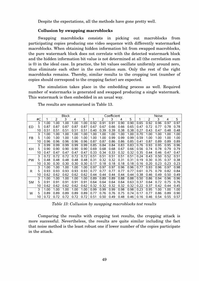
Despite the expectations, all the methods have gone pretty well.

Collusion by swapping macroblocks

Swapping macroblocks consists in picking out macroblocks from

participating copies producing one video sequence with differently watermarked

macroblocks. When obtaining hidden information bit from swapped macroblocks,

the pure watermark block does not correlate with the detected watermark block

and the hidden information bit value is not determined at all (the correlation sum

is 0) in the ideal case. In practice, the bit values oscillate uniformly around zero,

thus eliminate each other in the correlation sum. Only the rest of the right

macroblocks remains. Thereby, similar results to the cropping test (number of

copies should correspond to the cropping factor) are expected.

The simulation takes place in the embedding process as well. Required

number of watermarks is generated and swapped producing a single watermark.

This watermark is then embedded in an usual way.

The results are summarized in Table 13.

Table 13: Collusion by swapping macroblocks test results

Comparing the results with cropping test results, the cropping attack is

more successful. Nevertheless, the results are quite similar including the fact

that noise method is the least robust one if lower number of the copies participate

in the attack.

49

Block Coefficient Noise#C 1 2 3 4 5 1 2 3 4 5 1 2 3 4 5

ED3 1.00 1.00 1.00 1.00 1.00 0.92 0.91 0.91 0.90 0.90 0.65 0.92 0.96 0.97 0.975 0.87 0.87 0.87 0.87 0.87 0.67 0.67 0.66 0.66 0.65 0.47 0.72 0.77 0.78 0.7810 0.51 0.51 0.51 0.51 0.51 0.40 0.39 0.39 0.38 0.38 0.27 0.43 0.47 0.48 0.48

FB3 1.00 1.00 1.00 1.00 1.00 1.00 1.00 1.00 1.00 1.00 0.70 1.00 1.00 1.00 1.005 1.00 1.00 1.00 1.00 1.00 1.00 1.00 0.99 0.99 0.99 0.59 1.00 1.00 1.00 1.0010 0.96 0.96 0.96 0.96 0.96 0.87 0.87 0.86 0.86 0.85 0.41 0.87 0.89 0.89 0.89

KH3 0.99 0.99 0.99 0.99 0.99 0.85 0.84 0.84 0.83 0.83 0.76 0.93 0.95 0.95 0.965 0.90 0.90 0.90 0.90 0.90 0.69 0.68 0.68 0.67 0.66 0.56 0.74 0.78 0.79 0.7910 0.47 0.47 0.47 0.47 0.47 0.33 0.34 0.33 0.32 0.32 0.35 0.44 0.46 0.47 0.47

PW3 0.72 0.72 0.72 0.72 0.72 0.51 0.51 0.51 0.51 0.51 0.24 0.43 0.50 0.52 0.515 0.48 0.48 0.48 0.48 0.48 0.31 0.32 0.32 0.31 0.31 0.19 0.30 0.35 0.37 0.3810 0.30 0.30 0.30 0.30 0.30 0.17 0.18 0.18 0.18 0.18 0.16 0.20 0.23 0.23 0.23

R3 1.00 1.00 1.00 1.00 1.00 0.97 0.97 0.97 0.96 0.96 0.77 0.93 0.96 0.97 0.985 0.93 0.93 0.93 0.93 0.93 0.77 0.77 0.77 0.77 0.77 0.61 0.75 0.79 0.82 0.8410 0.62 0.62 0.62 0.62 0.62 0.44 0.44 0.44 0.44 0.44 0.38 0.46 0.49 0.50 0.49

SM3 1.00 1.00 1.00 1.00 1.00 0.89 0.89 0.89 0.88 0.88 0.50 0.86 0.94 0.96 0.965 0.91 0.91 0.91 0.91 0.91 0.64 0.64 0.64 0.64 0.63 0.37 0.64 0.72 0.75 0.7610 0.62 0.62 0.62 0.62 0.62 0.32 0.32 0.32 0.32 0.32 0.22 0.37 0.42 0.44 0.45

W3 1.00 1.00 1.00 1.00 1.00 0.99 0.99 0.99 0.98 0.98 0.23 0.95 1.00 1.00 1.005 0.89 0.89 0.89 0.89 0.89 0.77 0.76 0.76 0.75 0.74 0.17 0.77 0.86 0.89 0.9010 0.72 0.72 0.72 0.72 0.72 0.51 0.50 0.49 0.48 0.46 0.16 0.46 0.54 0.55 0.57

Chapter 6

Conclusion

Watermarking is a copy protection system that allows tracking back illegally

produced copies of the protected multimedia content. Compared with other copy

protection systems like Digital Rights Management, the main advantage of

watermarking is that the watermark is embedded permanently in visual data of

the content but at the cost of slight loss in fidelity.

In this thesis, three different watermarking methods have been designed

and implemented. Block and coefficient methods belong to watermarking

techniques in frequency domain while pseudo-random noise method represents

watermarking in spatial domain. Frequency domain techniques modify the

coefficients obtained by the application of some frequency transform to visual

data of the content. Spatial domain techniques apply the watermark directly to

visual data of the content.

A generic watermarking framework has been designed and implemented as

a plugin for an existing open source multimedia streaming library. The

framework provides the interface for easy implementation of particular

watermarking methods in both frequency and spatial domain.

The watermark embedding process is performed on a compressed video

stream. The H.264 video coding standard has been chosen as the particular video

compression technique. The standard uses a kind of the frequency transform

mentioned above, thus frequency domain watermarking is implemented using

coefficients of the compressed stream. The spatial domain watermark is

transformed to frequency domain using the transform before embedding.

The watermarking methods have been compared with each other in terms of

their perceptibility and robustness. The methods have been exposed to several

simulation tests checking up their resistance to various types of attacks.

All the methods are more or less resistant to simple attacks such as

50

recompression and noising, and to some removal attacks such as denoising and

collusion by averaging.

Noise method is the most resistant method to scaling. The watermark is

successfully detected even if the video is scaled down up to 1/5 of the former

resolution. Using any of the frequency domain methods, the watermark is

destroyed when scaling down the video to 1/3 of the former resolution.

On the other hand, noise method is the most vulnerable method to cropping.

The frequency domain methods withstand cropping the video up to 1/5 of the

former resolution while the watermark may be severely impaired by cropping the

video to 1/4 of the former resolution in case of noise method.

Concerning blurring, the noise method watermark is robust using any size

of the convolution blur mask. In case of both block and coefficient methods,

blurring with the 7×7 mask may destroy the watermark but the video quality is

severely degraded as well.

Sharpening even increases the watermark detection success probability in

all the methods.

When using the frequency domain methods, the multiple watermark

embedding test has shown that limited number of transform coefficients enables

overwriting of previously embedded watermarks. Thereby, an attacker may

completely destroy the former watermark.

On the other hand, the frequency domain methods are more resistant to

collusion by swapping macroblocks. Anyway, the watermark may be destroyed

with sufficient number of copies participating in the collusion attack.

Although noise method is more vulnerable to cropping, it is equally or more

resistant to the other attacks than the frequency domain methods. Moreover,

there is only few visual data left in the video cropped to 1/4 of the former

resolution.

Further, the noise method watermark is the least perceptible one in

comparison with the other method watermarks.

Unfortunately, there is a trade-off between benefits and much more bit-rate

growth when using noise method. Noise method increases the video bit-rate up to

two times more than the other methods, using reasonable weight factors. The

ratio grows up with increasing weight factor values.

With respect to the reasons above, noise watermarking method is

recommended despite the bit-rate growth. Further, weight factor of 2 is

recommended as a good compromise between robustness and perceptibility.

For practical use, several improvements should be made.

Firstly, the embedding process should be optimized to preserve the former

bit-rate of the video sequences.

51

In order to increase robustness against direct removal attack, the

watermark should be embedded into textured areas only. Textured areas provide

more non-zero coefficients in the residual than uniform areas do, thus the

watermark may be hidden more safely. Moreover, less distortion would be

produced.

Therefore, an adaptive embedding algorithm which would adjust the weight

factor per macroblock according to its complexity and spatial characteristics

should be implemented.

Furthermore, the distortion in inter predicted slices caused by prediction

from watermarked intra slices should be compensated. Among others, complete

inter prediction has to be implemented in order to accomplish this task.

As soon as the inter prediction error compensation is implemented, there is

only a small step left to implementation of the embedding process into inter coded

slices as well.

52

Bibliography

[1] Ingemar J. Cox, Joe Kilian, Tom Leighton and Talal Shamoon: A Secure,

Robust Watermark for Multimedia. Proceedings of the First International

Workshop on Information Hiding, 1996.

[2] Frank Hartung and Bernd Girod: Watermarking of Uncompressed and

Compressed Video. Signal Processing, 1998.

[3] V. Cappellini, F. Bartolini,R. Caldelli, A. De Rosa, A. Piva and M. Barni:

Robust Frame-based Watermarking for Digital Video. Proceedings of the

12th International Workshop on Database and Expert Systems

Applications, 2001.

[4] Hong-mei Liu, Ji-wu Huang and Zi-mei Xiao: An Adaptive Video

Watermarking Algorithm. International Conference on Multimedia and

Expo, 2001.

[5] B. Zhu, M. D. Swanson and A. H. Tewk: Multiresolution Scene-based Video

Watermarking Using Perceptual Models. IEEE Journal on Selected Areas in

Communications, 1998.

[6] Stefan Thiemert, Thomas Vogel, Jana Dittmann and Martin Steinebach: A

High-Capacity Block Based Video Watermark. Proceedings of the 30th

EUROMICRO Conference, 2004.

[7] Jun Zhang, Jiegu Li and Ling Zhang: Video Watermark Technique in Motion

Vector. Proceedings of the 14th Brazilian Symposium on Computer Graphics

and Image Processing, 2001.

[8] Frank Hartung, Jonathan K. Su and Bernd Girod: Spread Spectrum

Watermarking: Malicious Attacks and Counterattacks. Security and

Watermarking of Multimedia Contents, 1999.

[9] ITU-T Recommendation H.264: Advanced video coding for generic

audiovisual services, 2005.

[10] Oskar Flordal, Di Wu and Dake Liu: Accelerating CABAC Encoding for

Multi-standard Media with Configurability. Parallel and Distributed

Processing Symposium, 2006.

[11] ITU-T Recommendation H.264.1: Conformance specification for H.264

advanced video coding, 2005.

53

[12] GStreamer, http://gstreamer.freedesktop.org/

[13] H. Stone: Analysis of Attacks on Image Watermarks with Randomized

Coefficients. Technical report, NEC Research Institute, 1996.

[14] x264, http://www.videolan.org/developers/x264.html

[15] MPlayer, http://www.mplayerhq.hu/

[16] Apple - QuickTime - HD Gallery, http://www.apple.com/quicktime/guide/hd/

[17] Matroska, http://www.matroska.org/

[18] Elephants Dream, http://www.elephantsdream.org/

54

Appendix A

Enclosed CD & Installation

The source codes of the H.264 codec and of the watermarking plugin as well

as the third party software are provided on the enclosed CD. In particular, the

CD contains the following data:

detect Unix shell script that contains the detection GStreamer

pipeline

doxydoc/ programming documentation in the HTML format generated by

Doxygen from the source code of the plugin

embed Unix shell script that contains the embedding GStreamer

pipeline

gst-plugin source code of the watermarking plugin

h264 source code of the partial H.264 codec

installs/ source codes of GStreamer, MPlayer and x264

params additional Unix shell script used by the other scripts to parse

given command-line parameters

prepare Unix shell script that remuxes a video sequence in order to

contain intra coded slices only; the script is used by test scripts

tests/ Unix shell scripts that contain the simulation tests

thesis/ sources of the thesis

thesis.pdf the thesis in Acrobat PDF format

thesis.ps the thesis in PostScript format

video/ testing video sequences where the licence permits copying

All programs and libraries, provided in source code, may be installed on

Unix platforms in the following way. Copy the source code or the tarball to some

location where you have writing rights, and change the working directory to that

location. If the program is compressed as a tarball, type the following command

to obtain the source code:

tar xjvf <tarball.tar.bz2>

55

All the programs use the standard Unix build system, thus type

subsequently in the directories containing the programs:

./autogen.sh (in case there is no configure script)

./configure

make

make install

Some of the programs may require newer versions of libraries you have

installed. The configure script should detect this and report a message. In such

a case, please update the reported library.

Nevertheless, install the programs in the following order:

� GStreamer (tarball gstreamer-0.10.11.tar.bz2)

� GStreamer Base Plugins (tarball gst-plugins-base-0.10.11.tar.bz2)

� GStreamer Good Plugins (tarball gst-plugins-good-0.10.5.tar.bz2)

� the H.264 codec

� the watermarking plugin

And if you intend to execute the test scripts, install in addition:

� MPlayer (tarball MPlayer-1.0rc1.tar.bz2)

� x264 encoder (tarball x264-645.tar.bz2)

56

Appendix B

The plugin usage

The watermarking plugin can be used as an element queued in a GStreamer

pipeline. The construction of the pipelines is described in the documentation on

the project's website [12]. The name of the plugin is h264watermark.

The plugin behaviour is controlled by several parameters. The list of the

parameters follows:

mode specifies the working mode of the plugin. Three values may be assigned:

prepare (everything except parameter set NAL units and intra coded slices is

dropped), embed (activates the embedding process) and detect (activates the

detection process).

method selects the watermarking method: block, coeff (stands for coefficient)

and noise.

weight sets the weight factor.

content-id stands for the identifier of the video content.

copy-id is the identifier of the content copy.

It is possible to obtain the parameter list by using one of GStreamer utilities

as well – type:

gst-inspect h264watermark

There are three scripts, containing complete GStreamer pipelines, provided

on the enclosed CD – embed, detect and prepare – using the plugin in the

corresponding mode. The required arguments are listed if the scripts are

executed without any arguments. The first two arguments stand for the input

and the output files. Only Matroska muxed video sequences are accepted. The

other arguments represent the plugin parameters.

57

Appendix C

Programming Documentation

There is the programming documentation, generated from the source code of

the plugin, on the enclosed CD but lacks description of adding another

watermarking method.

In order to add a new watermarking method into the watermarking

framework, several actions have to be taken:

� The identifier of the method has to be inserted into the list of available

methods. The list, named WatermarkMethod, is located in file watermark.h.

� The name and the description of the method have to be inserted into the list of

possible values of the plugin's parameter method. The list is located in file

gsth264watermark.c and its name is mode_types.

� Both embedding and detection functions have to be implemented. The file that

contains the functions should be listed in file Makefile.am and the header

file with the function declarations should be included in file watermark.c.

The embedding and the detection functions have to be specified as the second

and the third item in the defining structure in the list of defining structures.

The list, named methods, is located in file watermark.c. The first item of

the structure is the type of watermarking domain that the method uses; it is

either WATERMARK_DOMAIN_FREQUENCY or WATERMARK_DOMAIN_SPATIAL.

Both the embedding and the detection functions in frequency domain have

the same arguments in the following order:

watermark is pointer to the framework context.

coefficients is pointer to the list of transform coefficients of one block. The

list contains zig-zag scan of the coefficients in case of frame macroblocks, or

field scan in case of field macroblocks.

58

length is the length of the list of coefficients.

CurrMbAddr is address of the macroblock that contains the block. The address is

the index of the macroblock in macroblock raster scan.

y is row index of the top-left pixel of the block within the picture.

x is column index of the top-left pixel of the block within the picture.

The embedding function in spatial domain has the same arguments but

there are residual and dimension arguments instead of coefficients and

length:

residual is 2-dimensional array of residual values of one block.

dimension is dimension of the block.

Finally, there is a picture argument instead of residual in case of the

detection function in spatial domain. The picture argument stands for a block of

luma samples located at the position specified by x and y.

In case the embedding function in spatial domain requires luma samples of

the block besides the residual, the whole picture is available in item

picture_original in the framework context.

59