VICTOR JUAREZ-LERIA

TIMING-BASED LOCATION ESTIMATION FOR OFDM SIGNALS

WITH APPLICATIONS IN LTE, WLAN AND WIMAX Master of Science Thesis

Examiners: Docent, Dr. Elena-Simona Lohan

Elina Laitinen

Examiners and topic approved by the Faculty

Council on 8th February 2012

i

Abstract

TAMPERE UNIVERSITY OF TECHNOLOGY Erasmus Programme JUAREZ-LERIA, VICTOR: Timing-Based Location Estimation for OFDM Signals with Applications in LTE, WLAN and WiMAX Master of Science Thesis, 60 pages, 5 Appendix pages March 2012 Examiner: Elena-Simona Lohan and Elina Laitinen Keywords: Orthogonal Frequency Division Multiplexing, preamble, synchronization.

Orthogonal Frequency Division Multiplexing (OFDM) has gained importance in recent

years and it is the technique selected for wireless systems, such as Long-Term Evolution

(LTE) for 4G communications systems, Wireless Local Area Networks (WLAN) or

WiMAXTM

. For this reason, OFDM systems have been under study in order to develop

more accurate mobile stations positioning, both in outdoors and indoors environments.

Nevertheless, OFDM systems require high timing synchronization accuracy in order to be

able to receive the signal correctly, which makes timing synchronization estimation a key

issue in OFDM receivers. Propagation is especially complicated over wireless channels,

where the presence of multipath propagation, high level of interference signals or the

obstruction of Line Of Sight (LOS) path make timing estimation even more difficult in

indoor environments.

The research results presented in this thesis focus on the study of different coarse

positioning techniques for wireless networks using OFDM signals, for various static single

path channels and fading multipath channels. The methods under study are based on timing

synchronization algorithms and various preambles embedded in the OFDM signal. Also

Correlation-Based Timing Synchronization estimators (CBTS) and Multiple Signal

Classification (MUSIC) approaches are investigated. The performance of the studied

estimation algorithms is analyzed in terms of Root Mean Square Error (RMSE), obtained

from computer simulation results and the aim is to provide a detailed comparison of

various OFDM preamble-based timing estimators.

ii

Table of Contents

ABSTRACT ...................................................................................................................................................... I

TABLE OF CONTENTS ............................................................................................................................... II

LIST OF SYMBOLS ..................................................................................................................................... IV

LIST OF ACRONYMS ................................................................................................................................. VI

1 INTRODUCTION .................................................................................................................................. 1

1.1 BACKGROUND .................................................................................................................................. 1

1.2 THESIS OBJECTIVE AND CONTRIBUTIONS ......................................................................................... 2

1.3 THESIS ORGANIZATION ..................................................................................................................... 3

2 THE OFDM CONCEPT ........................................................................................................................ 4

2.1 LONG TERM EVOLUTION .................................................................................................................. 6

2.1.1 Physical channels ........................................................................................................................ 6

2.1.2 Modulation types ......................................................................................................................... 9

2.1.3 LTE Frame structure ................................................................................................................. 11

2.2 WIRELESS LOCAL AREA NETWORKS .............................................................................................. 12

2.2.1 Modulation types ....................................................................................................................... 12

2.2.2 802.11n standard ....................................................................................................................... 12

2.2.3 802.11b/g standard .................................................................................................................... 13

2.3 WIMAX ......................................................................................................................................... 13

2.4 POWER SPECTRAL DENSITY ............................................................................................................. 14

2.5 PARAMETERS OF THE DIFFERENT SYSTEMS ..................................................................................... 17

3 LOCATION PRINCIPLES ................................................................................................................. 18

3.1 RECEIVED SIGNAL STRENGTH (RSS) .............................................................................................. 18

3.2 TIME OF ARRIVAL (TOA) ............................................................................................................... 19

3.3 TIME DIFFERENCE OF ARRIVAL (TDOA) ....................................................................................... 19

3.4 ANGLE OF ARRIVAL (AOA) ........................................................................................................... 20

4 TIMING ESTIMATION WITH OFDM............................................................................................. 22

4.1 CORRELATION-BASED TIMING SYNCHRONIZATION ......................................................................... 22

4.2 PREAMBLE-BASED .......................................................................................................................... 22

4.2.1 Schmidl preamble ...................................................................................................................... 22

4.2.2 Minn metric ............................................................................................................................... 24

4.2.3 Park preamble ........................................................................................................................... 26

4.2.4 Kim preamble ............................................................................................................................ 27

4.2.5 Ren preamble ............................................................................................................................. 29

4.2.6 Kang preamble .......................................................................................................................... 30

4.3 MULTIPLE SIGNAL CLASSIFICATION ................................................................................................ 32

5 SIMULATION MODEL ...................................................................................................................... 34

iii

6 SIMULATION RESULTS FOR TIMING ......................................................................................... 36

6.1 COMPARISON FOR VARIOUS SNR VALUES ...................................................................................... 36

6.2 COMPARISON FOR VARIOUS NUMBER OF SUB-CARRIERS ................................................................. 40

6.3 COMPARISON FOR VARIOUS GUARD INTERVAL LENGTHS ................................................................ 44

6.4 COMPARISON FOR VARIOUS OFDM SYMBOL TIMES ....................................................................... 45

7 CONCLUSIONS AND OPEN ISSUES ............................................................................................... 47

REFERENCES .............................................................................................................................................. 49

APPENDIX .................................................................................................................................................... 53

iv

List of symbols

a(hm) Correction factor for hm

bi i-th BS

��� p-th complex data symbol of the k-th OFDM symbol

����� n-th sample of Zadoff-Chu sequence

∆f Sub-carrier spacing

∆Θ Οrientation of the unknown mobile station

∆PRS PRS sub-frames offset

∆ Normalized difference between the theoretical and real start of an OFDM

�� Measurement uncertainty

fc Carrier frequency

��� Carrier frequency offset

h(t) Channel impulsive response

hb BS effective antenna height

hm MS antenna height

IPRS PRS configuration index

N Number of subcarriers

Ncp Samples of the CP

NPRS PRS sub-frames

NFFT FFT length

n(t) AWGN

Θi i-th relative AOAs of the sent signals from bi

�� i-th BS position

v

�� MS position

r(t) Received signal

s(t) Emitted signal

��� n-th sample of the k-th emitted OFDM symbol.

�� Useful length of an OFDM symbol

�� CP time length

TPRS PRS period

����� Sampling time

u Unknown MS

��� Generic time measurement relative to reference point i

vi

List of acronyms

AOA Angle of Arrival

AP Access Point

ARQ Auto Repeat Request

AWGN Additive White Gaussian Noise

BS Base Station

BPSK Binary Phase Shift Keying

CAZAC Constant Amplitude Zero Auto-Correlation

CBTS Correlation Based Timing Synchronization

CP Cyclic Prefix

CSP Correlation Sequence of the Preamble

DC Direct Current

DFT Discrete Fourier Transformation

DwPTS Downlink Pilot Signal

FDD Frequency Division Duplex

GI Guard Interval

GNSS Galileo Navigation Satellite System

GP Guard Period

GPS Global Positioning System

ICI Inter-Carrier Interference

IDFT Inverse Discrete Fourier Transformation

IFFT Inverse Fast Fourier Transformation

LTE Long Term Evolution

vii

MBSDN Multimedia Broadcast over Single Frequency Network

MS Mobile Station

MUSIC Multiple Signal Classification

NLOS Non Line Of Sight

OFDM Orthogonal Frequency Division Multiplexing

PN Pseudo Noise

PRS Positioning Reference Signal

PSD Power Spectral Density

QAM Quadrature Amplitude Modulation

QPSK Quadrature Phase Shift Keying

RSS Received Signal Strength

SC-FDMA Single Carrier – Frequency Division Multiplexing Access

SNR Signal to Noise Ratio

SoO Signals of Opportunity

TDD Time Division Duplex

TDOA Time Difference Of Arrival

TOA Time Of Arrival

UE User Equipment

WLAN Wireless Local Area Networks

WMAN Wireless Metropolitan Area Networks

1

1 Introduction

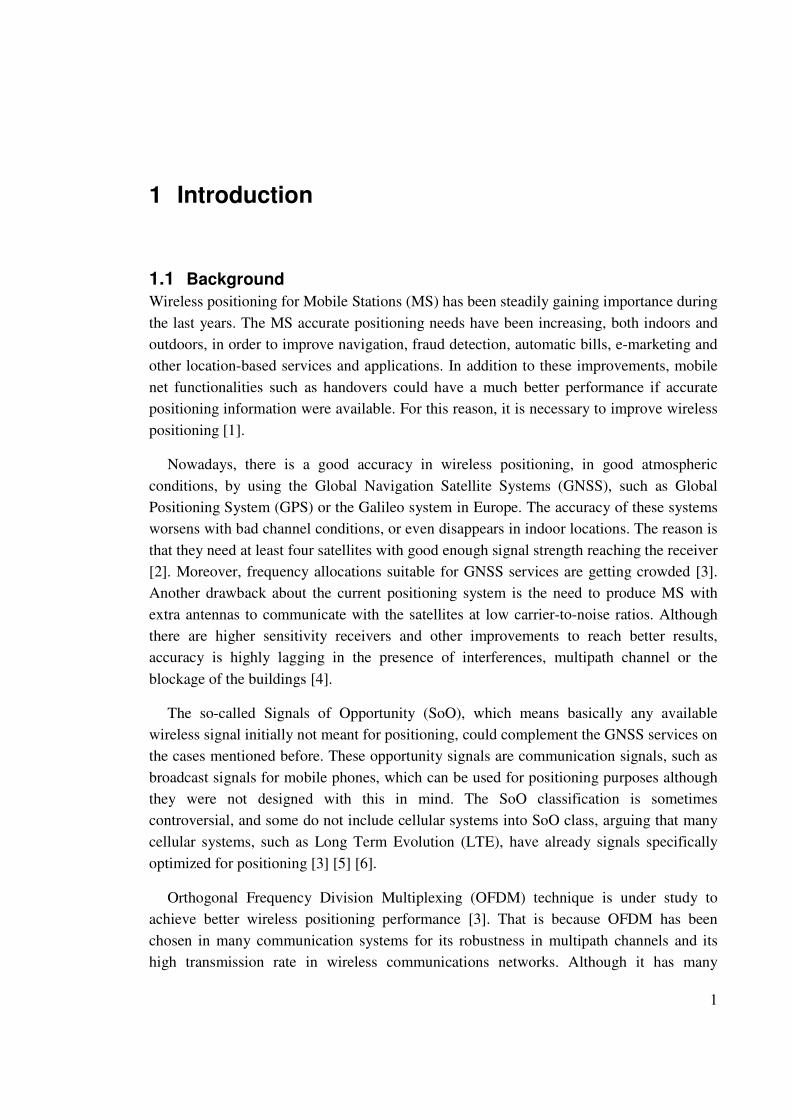
1.1 Background

Wireless positioning for Mobile Stations (MS) has been steadily gaining importance during

the last years. The MS accurate positioning needs have been increasing, both indoors and

outdoors, in order to improve navigation, fraud detection, automatic bills, e-marketing and

other location-based services and applications. In addition to these improvements, mobile

net functionalities such as handovers could have a much better performance if accurate

positioning information were available. For this reason, it is necessary to improve wireless

positioning [1].

Nowadays, there is a good accuracy in wireless positioning, in good atmospheric

conditions, by using the Global Navigation Satellite Systems (GNSS), such as Global

Positioning System (GPS) or the Galileo system in Europe. The accuracy of these systems

worsens with bad channel conditions, or even disappears in indoor locations. The reason is

that they need at least four satellites with good enough signal strength reaching the receiver

[2]. Moreover, frequency allocations suitable for GNSS services are getting crowded [3].

Another drawback about the current positioning system is the need to produce MS with

extra antennas to communicate with the satellites at low carrier-to-noise ratios. Although

there are higher sensitivity receivers and other improvements to reach better results,

accuracy is highly lagging in the presence of interferences, multipath channel or the

blockage of the buildings [4].

The so-called Signals of Opportunity (SoO), which means basically any available

wireless signal initially not meant for positioning, could complement the GNSS services on

the cases mentioned before. These opportunity signals are communication signals, such as

broadcast signals for mobile phones, which can be used for positioning purposes although

they were not designed with this in mind. The SoO classification is sometimes

controversial, and some do not include cellular systems into SoO class, arguing that many

cellular systems, such as Long Term Evolution (LTE), have already signals specifically

optimized for positioning [3] [5] [6].

Orthogonal Frequency Division Multiplexing (OFDM) technique is under study to

achieve better wireless positioning performance [3]. That is because OFDM has been

chosen in many communication systems for its robustness in multipath channels and its

high transmission rate in wireless communications networks. Although it has many

2

advantages, it has some disadvantages as well. Firstly, OFDM is seriously affected by

synchronization errors. Moreover, the OFDM signal has a noise like amplitude with a very

large dynamic range; therefore it requires RF power amplifiers with a high peak to average

power ratio. OFDM is also more sensitive to carrier frequency offset and drift than single

carrier systems are due to leakage of the Discrete Fourier Transformation (DFT) [7] [2] [8]

[9].

1.2 Thesis Objective and Contributions

Because of OFDM systems require high timing synchronization accuracy to be able to

receive the signal correctly, it will be necessary to work with algorithms to estimate

symbol timing of the received signal. Once the timing estimation is correct, the delay of

the signal from the Base Station (BS) to the MS can be found and, consequently, the

distances between said stations can be calculated in order to obtain the mobile terminal

position.

There are two classes of OFDM timing synchronization. The first class of timing

synchronization algorithms is based on adding a specific preamble, which is different in

each case, before the useful data. The second class uses pilot embedded in the data and

correlation or covariance matrix information in order to estimate the unknown timing, both

approaches (non-data aided and data aided) are investigated in this thesis. The main

objective has been to investigate the accuracy limits of various preamble-based and non-

preamble-based timing synchronization algorithms, both in single path and multipath

channels for OFDM signals. The algorithms are compared by simulating some possible

environments and analyzing the errors they perform, in meters, while some system

parameters are changed. The author has contributed to the followings:

- Literature study of various preamble-based and non-preamble-based timing

synchronization algorithms in OFDM

- Implementation (in Matlab) of the following preamble-based algorithms: Schmidl,

Minn, Park, Kim, Ren and Kang, starting from the ideas presented in [10] [11] [12]

[13] [14] [15].

- Implementation (in Matlab) of CBTS and MUSIC estimators.

- Comparison of various timing estimation algorithms in single path (static) and

multipath (fading) channels.

The work has done during the period September 2011-March 2012 at the Department of

Communications Engineering, Tampere University of Technology (TUT), Finland, during

an Erasmus exchange visit.

3

1.3 Thesis Organization

The thesis is organized in seven chapters. The OFDM concept is presented in Chapter 2,

including three systems that use it (LTE, WLAN and WiMAX). In Chapter 3, the four

main location techniques are briefly explained. Once we focus on a specific location

technique, namely the timing-based localization, the different algorithms for timing

synchronization are presented in Chapter 4. In Chapter 5, there is a description of the

developed Matlab simulation model. In Chapter 6, there is an explanation of simulation

results comparing all estimation algorithms. Chapter 7 focuses on conclusions and open

issues. The thesis also has an Appendix illustrating some of the m-codes implemented by

the Author.

4

2 The OFDM concept

The OFDM technique consists of transmitting N complex data symbols over N narrow and

orthogonal subcarriers. These subcarriers can be superposed without interfering thanks to

being orthogonal, which means that there is no Inter-Carrier Interference (ICI) when the

receiver is synchronized. The mentioned subcarriers are chosen narrow enough so they can

be considered as belonging to flat regions, and they can be easily equalized to correct the

errors at the receiver. Moreover, the transmission rate is higher due to the parallel sub-

carriers sending information at the same time [16].

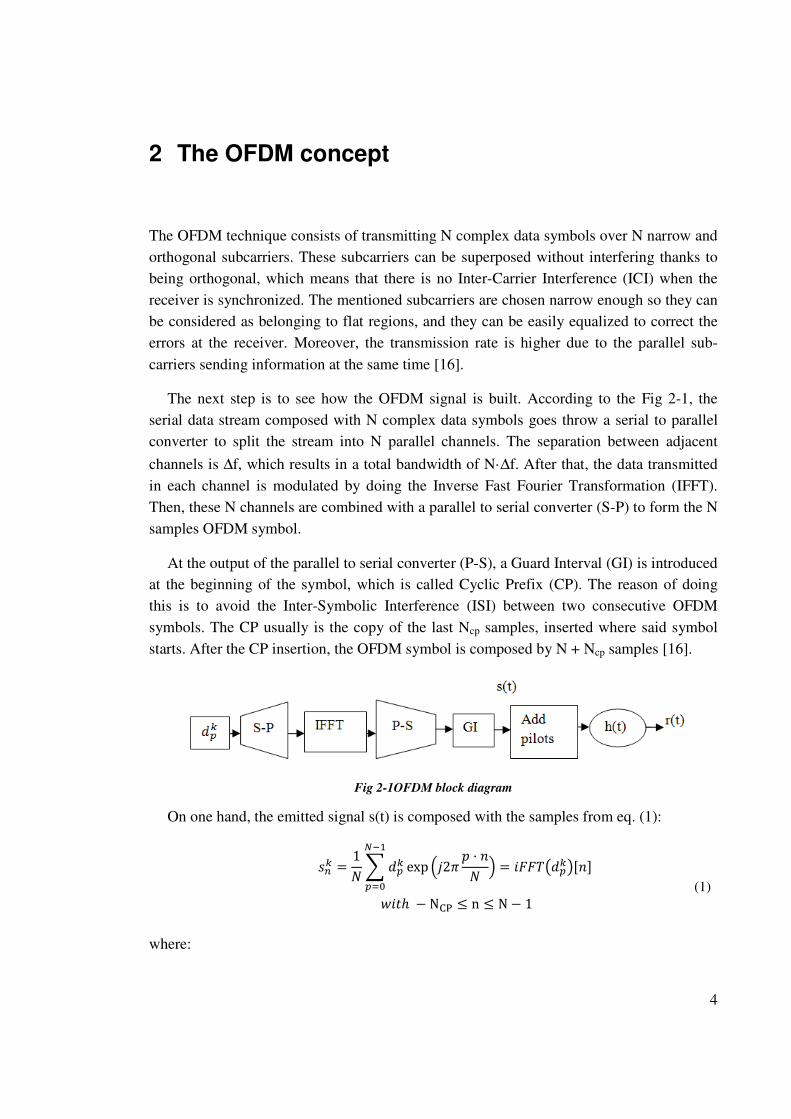
The next step is to see how the OFDM signal is built. According to the Fig 2-1, the

serial data stream composed with N complex data symbols goes throw a serial to parallel

converter to split the stream into N parallel channels. The separation between adjacent

channels is ∆f, which results in a total bandwidth of N·∆f. After that, the data transmitted

in each channel is modulated by doing the Inverse Fast Fourier Transformation (IFFT).

Then, these N channels are combined with a parallel to serial converter (S-P) to form the N

samples OFDM symbol.

At the output of the parallel to serial converter (P-S), a Guard Interval (GI) is introduced

at the beginning of the symbol, which is called Cyclic Prefix (CP). The reason of doing

this is to avoid the Inter-Symbolic Interference (ISI) between two consecutive OFDM

symbols. The CP usually is the copy of the last Ncp samples, inserted where said symbol

starts. After the CP insertion, the OFDM symbol is composed by N + Ncp samples [16].

Fig 2-1OFDM block diagram

On one hand, the emitted signal s(t) is composed with the samples from eq. (1):

��� = 1� � ��� exp"#2% � · �� '()*�+, = -..�/���01�2

3-4ℎ − N89 ≤ n ≤ N− 1

(1)

where:

5

- n is the sample time index.

- p is the subcarrier index.

- k is the OFDM symbol number.

- ��� is the p-th complex data symbol of the k-th OFDM symbol.

- ��� is the n-th sample of the k-th emitted OFDM symbol.

The last step before sending the OFDM signal through the channel consists on adding

some pilot signals.

On the other hand, the received signal is defined in eq. (2):

<�4� = /��4� ∗ ℎ�4�0/4 − ∆ · �����0>��#2% ����� 4� + ��4� (2)

where:

- ��� is the carrier frequency offset, which occurs when the received signal is

not synchronized.

- ∆ is the difference between the theoretical and real start of an OFDM symbol,

normalized to the sampling period, �����.

- ��is the useful length of an OFDM symbol.

- ℎ�4�isthechannelimpulseresponse.

- ��4� is Additive White Gaussian Noise (AWGN).

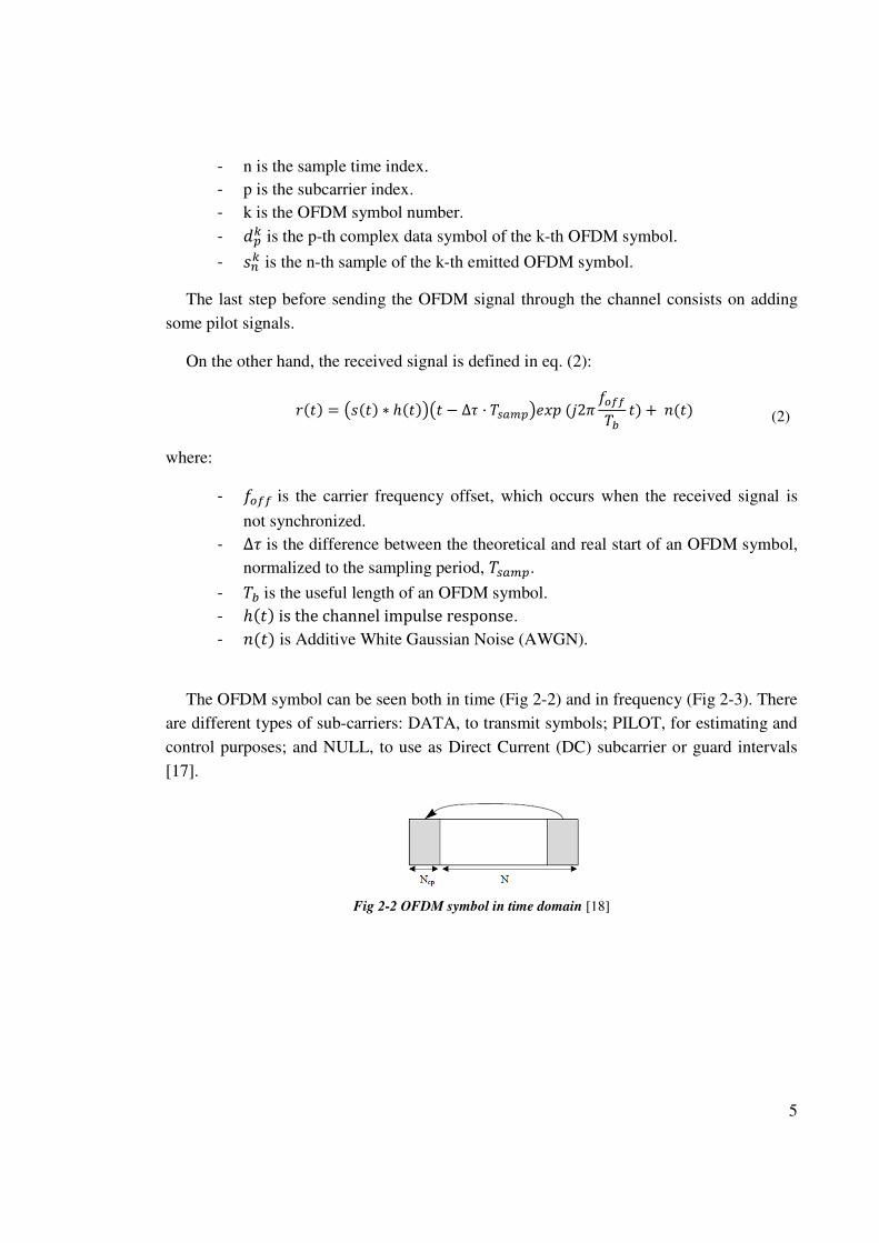
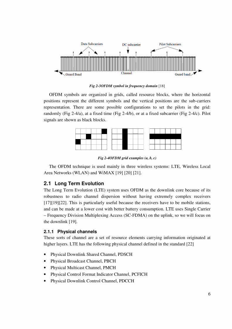
The OFDM symbol can be seen both in time (Fig 2-2) and in frequency (Fig 2-3). There

are different types of sub-carriers: DATA, to transmit symbols; PILOT, for estimating and

control purposes; and NULL, to use as Direct Current (DC) subcarrier or guard intervals

[17].

Fig 2-2 OFDM symbol in time domain [18]

6

Fig 2-3OFDM symbol in frequency domain [18]

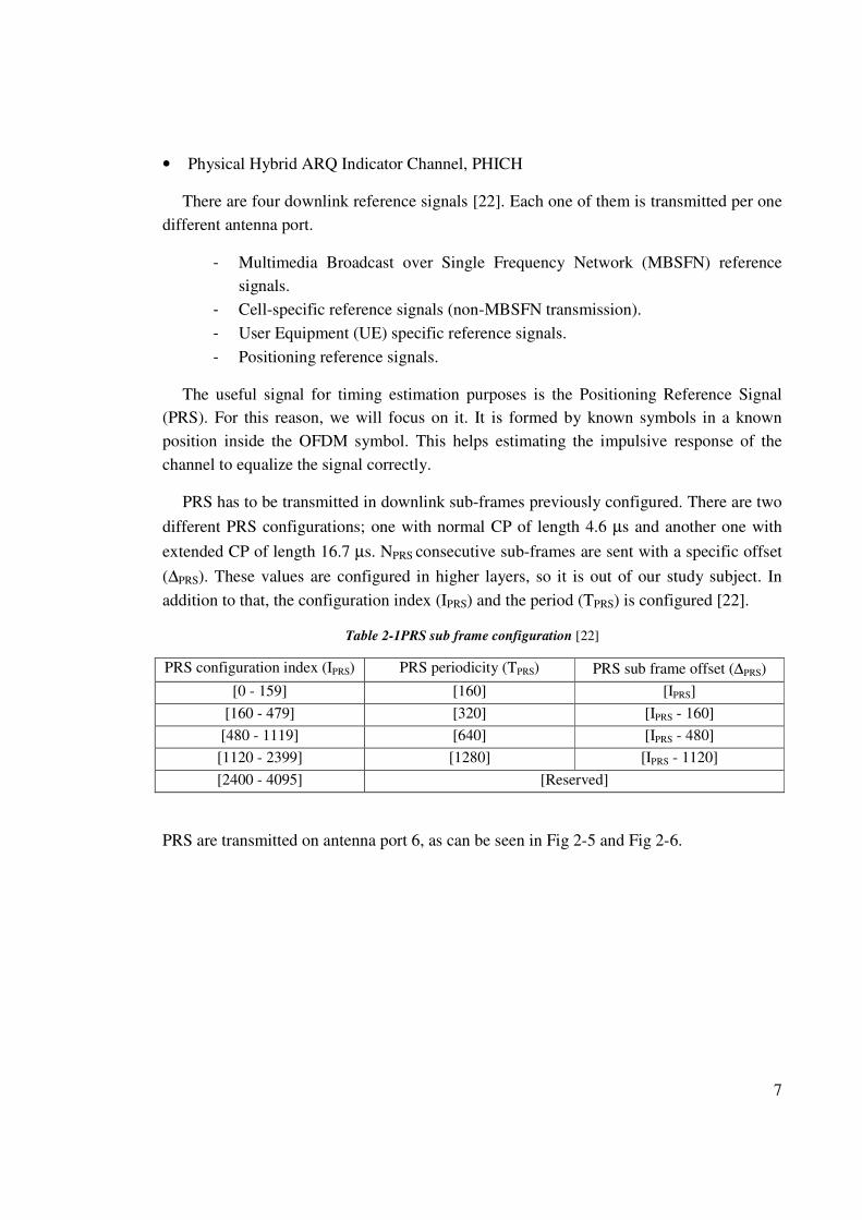
OFDM symbols are organized in grids, called resource blocks, where the horizontal

positions represent the different symbols and the vertical positions are the sub-carriers

representation. There are some possible configurations to set the pilots in the grid:

randomly (Fig 2-4/a), at a fixed time (Fig 2-4/b), or at a fixed subcarrier (Fig 2-4/c). Pilot

signals are shown as black blocks.

Fig 2-4OFDM grid examples (a, b, c)

The OFDM technique is used mainly in three wireless systems: LTE, Wireless Local

Area Networks (WLAN) and WiMAX [19] [20] [21].

2.1 Long Term Evolution

The Long Term Evolution (LTE) system uses OFDM as the downlink core because of its

robustness to radio channel dispersion without having extremely complex receivers

[17][19][22]. This is particularly useful because the receivers have to be mobile stations,

and can be made at a lower cost with better battery consumption. LTE uses Single Carrier

– Frequency Division Multiplexing Access (SC-FDMA) on the uplink, so we will focus on

the downlink [19].

2.1.1 Physical channels

These sorts of channel are a set of resource elements carrying information originated at

higher layers. LTE has the following physical channel defined in the standard [22]

• Physical Downlink Shared Channel, PDSCH

• Physical Broadcast Channel, PBCH

• Physical Multicast Channel, PMCH

• Physical Control Format Indicator Channel, PCFICH

• Physical Downlink Control Channel, PDCCH

7

• Physical Hybrid ARQ Indicator Channel, PHICH

There are four downlink reference signals [22]. Each one of them is transmitted per one

different antenna port.

- Multimedia Broadcast over Single Frequency Network (MBSFN) reference

signals.

- Cell-specific reference signals (non-MBSFN transmission).

- User Equipment (UE) specific reference signals.

- Positioning reference signals.

The useful signal for timing estimation purposes is the Positioning Reference Signal

(PRS). For this reason, we will focus on it. It is formed by known symbols in a known

position inside the OFDM symbol. This helps estimating the impulsive response of the

channel to equalize the signal correctly.

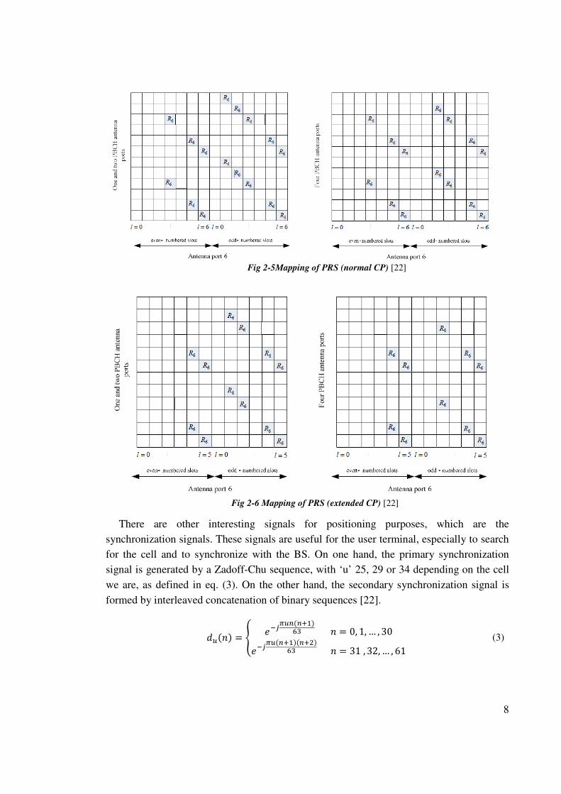
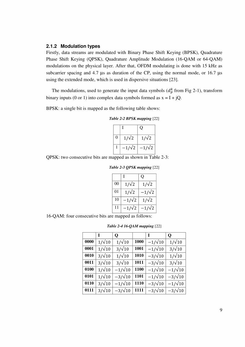
PRS has to be transmitted in downlink sub-frames previously configured. There are two

different PRS configurations; one with normal CP of length 4.6 µs and another one with

extended CP of length 16.7 µs. NPRS consecutive sub-frames are sent with a specific offset

(∆PRS). These values are configured in higher layers, so it is out of our study subject. In

addition to that, the configuration index (IPRS) and the period (TPRS) is configured [22].

Table 2-1PRS sub frame configuration [22]

PRS configuration index (IPRS) PRS periodicity (TPRS) PRS sub frame offset (∆PRS)

[0 - 159] [160] [IPRS]

[160 - 479] [320] [IPRS - 160]

[480 - 1119] [640] [IPRS - 480]

[1120 - 2399] [1280] [IPRS - 1120]

[2400 - 4095] [Reserved]

PRS are transmitted on antenna port 6, as can be seen in Fig 2-5 and Fig 2-6.

8

There are other interesting signals for positioning purposes, which are the

synchronization signals. These signals are useful for the user terminal, especially to search

for the cell and to synchronize with the BS. On one hand, the primary synchronization

signal is generated by a Zadoff-Chu sequence, with ‘u’ 25, 29 or 34 depending on the cell

we are, as defined in eq. (3). On the other hand, the secondary synchronization signal is

formed by interleaved concatenation of binary sequences [22].

����� = K )LM����N*�OP � = 0, 1, … , 30)LM���N*���NU�OP � = 31, 32,… , 61W (3)

Fig 2-5Mapping of PRS (normal CP) [22]

Fig 2-6 Mapping of PRS (extended CP) [22]

9

2.1.2 Modulation types

Firstly, data streams are modulated with Binary Phase Shift Keying (BPSK), Quadrature

Phase Shift Keying (QPSK), Quadrature Amplitude Modulation (16-QAM or 64-QAM)

modulations on the physical layer. After that, OFDM modulating is done with 15 kHz as

subcarrier spacing and 4.7 µs as duration of the CP, using the normal mode, or 16.7 µs

using the extended mode, which is used in dispersive situations [23].

The modulations, used to generate the input data symbols (��� from Fig 2-1), transform

binary inputs (0 or 1) into complex data symbols formed as x = I + jQ.

BPSK: a single bit is mapped as the following table shows:

Table 2-2 BPSK mapping [22]

I Q

0 1/√2 1/√2

1 −1/√2 −1/√2

QPSK: two consecutive bits are mapped as shown in Table 2-3:

Table 2-3 QPSK mapping [22]

I Q

00 1/√2 1/√2

01 1/√2 −1/√2

10 −1/√2 1/√2

11 −1/√2 −1/√2

16-QAM: four consecutive bits are mapped as follows:

Table 2-4 16-QAM mapping [22]

I Q I Q

0000 1/√10 1/√10 1000 −1/√10 1/√10

0001 1/√10 3/√10 1001 −1/√10 3/√10

0010 3/√10 1/√10 1010 −3/√10 1/√10

0011 3/√10 3/√10 1011 −3/√10 3/√10

0100 1/√10 −1/√10 1100 −1/√10 −1/√10

0101 1/√10 −3/√10 1101 −1/√10 −3/√10

0110 3/√10 −1/√10 1110 −3/√10 −1/√10

0111 3/√10 −3/√10 1111 −3/√10 −3/√10

10

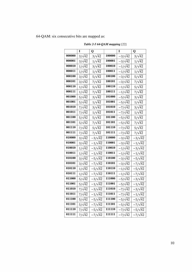
64-QAM: six consecutive bits are mapped as:

Table 2-5 64-QAM mapping [22]

I Q I Q

000000 3/√42 3/√42 100000 −3/√42 3/√42

000001 3/√42 1/√42 100001 −3/√42 1/√42

000010 1/√42 3/√42 100010 −1/√42 3/√42

000011 1/√42 1/√42 100011 −1/√42 1/√42

000100 3/√42 5/√42 100100 −3/√42 5/√42

000101 3/√42 7/√42 100101 −3/√42 7/√42

000110 1/√42 5/√42 100110 −1/√42 5/√42

000111 1/√42 7/√42 100111 −1/√42 7/√42

001000 5/√42 3/√42 101000 −5/√42 3/√42

001001 5/√42 1/√42 101001 −5/√42 1/√42

001010 7/√42 3/√42 101010 −7/√42 3/√42

001011 7/√42 1/√42 101011 −7/√42 1/√42

001100 5/√42 5/√42 101100 −5/√42 5/√42

001101 5/√42 7/√42 101101 −5/√42 7/√42

001110 7/√42 5/√42 101110 −7/√42 5/√42

001111 7/√42 7/√42 101111 −7/√42 7/√42

010000 3/√42 −3/√42 110000 −3/√42 −3/√42

010001 3/√42 −1/√42 110001 −3/√42 −1/√42

010010 1/√42 −3/√42 110010 −1/√42 −3/√42

010011 1/√42 −1/√42 110011 −1/√42 −1/√42

010100 3/√42 −5/√42 110100 −3/√42 −5/√42

010101 3/√42 −7/√42 110101 −3/√42 −7/√42

010110 1/√42 −5/√42 110110 −1/√42 −5/√42

010111 1/√42 −7/√42 110111 −1/√42 −7/√42

011000 5/√42 −3/√42 111000 −5/√42 −3/√42

011001 5/√42 −1/√42 111001 −5/√42 −1/√42

011010 7/√42 −3/√42 111010 −7/√42 −3/√42

011011 7/√42 −1/√42 111011 −7/√42 −1/√42

011100 5/√42 −5/√42 111100 −5/√42 −5/√42

011101 5/√42 −7/√42 111101 −5/√42 −7/√42

011110 7/√42 −5/√42 111110 −7/√42 −5/√42

011111 7/√42 −7/√42 111111 −7/√42 −7/√42

11

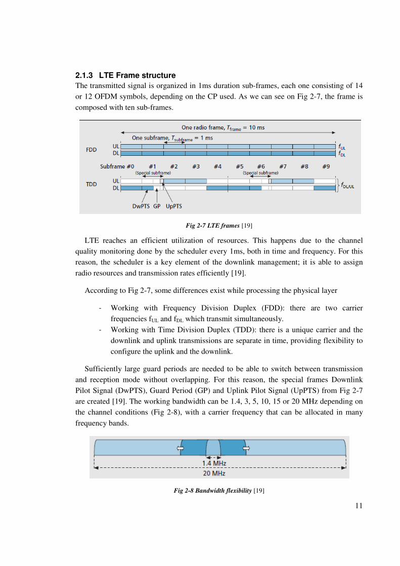
2.1.3 LTE Frame structure

The transmitted signal is organized in 1ms duration sub-frames, each one consisting of 14

or 12 OFDM symbols, depending on the CP used. As we can see on Fig 2-7, the frame is

composed with ten sub-frames.

Fig 2-7 LTE frames [19]

LTE reaches an efficient utilization of resources. This happens due to the channel

quality monitoring done by the scheduler every 1ms, both in time and frequency. For this

reason, the scheduler is a key element of the downlink management; it is able to assign

radio resources and transmission rates efficiently [19].

According to Fig 2-7, some differences exist while processing the physical layer

- Working with Frequency Division Duplex (FDD): there are two carrier

frequencies fUL and fDL which transmit simultaneously.

- Working with Time Division Duplex (TDD): there is a unique carrier and the

downlink and uplink transmissions are separate in time, providing flexibility to

configure the uplink and the downlink.

Sufficiently large guard periods are needed to be able to switch between transmission

and reception mode without overlapping. For this reason, the special frames Downlink

Pilot Signal (DwPTS), Guard Period (GP) and Uplink Pilot Signal (UpPTS) from Fig 2-7

are created [19]. The working bandwidth can be 1.4, 3, 5, 10, 15 or 20 MHz depending on

the channel conditions (Fig 2-8), with a carrier frequency that can be allocated in many

frequency bands.

Fig 2-8 Bandwidth flexibility [19]

12

2.2 Wireless Local Area Networks

Another system that uses OFDM technique is Wireless Local Area Networks (WLAN) or

802.11 family [20]. In what follows, we will focus on the most used systems nowadays,

namely 802.11b/g and 802.11n.

2.2.1 Modulation types

The modulations used, both in 802.11n and 802.11b/g, are BPSK, QPSK, 16-QAM and 64-

QAM depending on the environmental conditions [26]. These modulations are explained in

section 2.1.2.

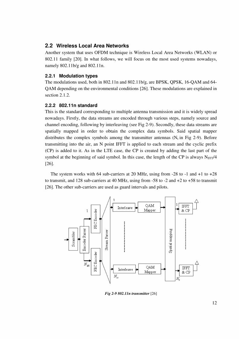
2.2.2 802.11n standard

This is the standard corresponding to multiple antenna transmission and it is widely spread

nowadays. Firstly, the data streams are encoded through various steps, namely source and

channel encoding, following by interleaving (see Fig 2-9). Secondly, these data streams are

spatially mapped in order to obtain the complex data symbols. Said spatial mapper

distributes the complex symbols among the transmitter antennas (Nt in Fig 2-9). Before

transmitting into the air, an N point IFFT is applied to each stream and the cyclic prefix

(CP) is added to it. As in the LTE case, the CP is created by adding the last part of the

symbol at the beginning of said symbol. In this case, the length of the CP is always NFFT/4

[26].

The system works with 64 sub-carriers at 20 MHz, using from -28 to -1 and +1 to +28

to transmit, and 128 sub-carriers at 40 MHz, using from -58 to -2 and +2 to +58 to transmit

[26]. The other sub-carriers are used as guard intervals and pilots.

Fig 2-9 802.11n transmitter [26]

13

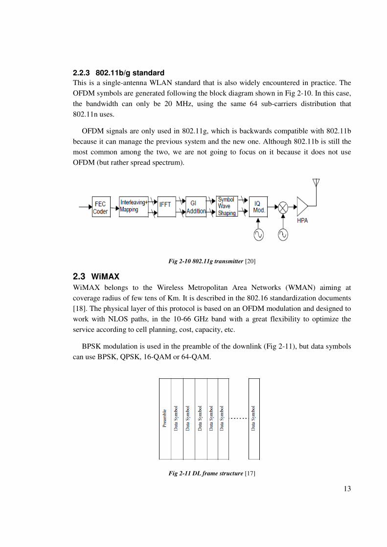
2.2.3 802.11b/g standard

This is a single-antenna WLAN standard that is also widely encountered in practice. The

OFDM symbols are generated following the block diagram shown in Fig 2-10. In this case,

the bandwidth can only be 20 MHz, using the same 64 sub-carriers distribution that

802.11n uses.

OFDM signals are only used in 802.11g, which is backwards compatible with 802.11b

because it can manage the previous system and the new one. Although 802.11b is still the

most common among the two, we are not going to focus on it because it does not use

OFDM (but rather spread spectrum).

Fig 2-10 802.11g transmitter [20]

2.3 WiMAX

WiMAX belongs to the Wireless Metropolitan Area Networks (WMAN) aiming at

coverage radius of few tens of Km. It is described in the 802.16 standardization documents

[18]. The physical layer of this protocol is based on an OFDM modulation and designed to

work with NLOS paths, in the 10-66 GHz band with a great flexibility to optimize the

service according to cell planning, cost, capacity, etc.

BPSK modulation is used in the preamble of the downlink (Fig 2-11), but data symbols

can use BPSK, QPSK, 16-QAM or 64-QAM.

Fig 2-11 DL frame structure [17]

14

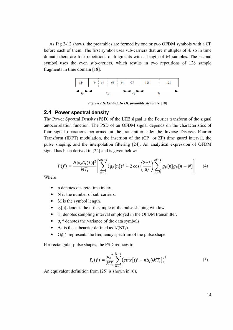
As Fig 2-12 shows, the preambles are formed by one or two OFDM symbols with a CP

before each of them. The first symbol uses sub-carriers that are multiples of 4, so in time

domain there are four repetitions of fragments with a length of 64 samples. The second

symbol uses the even sub-carriers, which results in two repetitions of 128 sample

fragments in time domain [18].

Fig 2-12 IEEE 802.16 DL preamble structure [18]

2.4 Power spectral density

The Power Spectral Density (PSD) of the LTE signal is the Fourier transform of the signal

autocorrelation function. The PSD of an OFDM signal depends on the characteristics of

four signal operations performed at the transmitter side: the Inverse Discrete Fourier

Transform (IDFT) modulation, the insertion of the (CP or ZP) time guard interval, the

pulse shaping, and the interpolation filtering [24]. An analytical expression of OFDM

signal has been derived in [24] and is given below:

]� � = �|_`a�� �|Ub�� c � �de1�2�U + 2 cos f2% ∆� g � de1�2de1� − �2h)*�+(

U()*�+, i (4)

Where

• n denotes discrete time index.

• N is the number of sub-carriers.

• M is the symbol length.

• gP[n] denotes the n-th sample of the pulse shaping window.

• Ts denotes sampling interval employed in the OFDM transmitter.

• _`U denotes the variance of the data symbols.

• ∆f is the subcarrier defined as 1/(NTs).

• Gi(f) represents the frequency spectrum of the pulse shape.

For rectangular pulse shapes, the PSD reduces to:

]j� � = _`Ub�� �/�-�kl� − �∆��b��m0U()*�+, (5)

An equivalent definition from [25] is shown in (6).

15

]� � = n� � op� − q∆��oU( Ur

�+)( Ur, q = ±1,±2,… ,±�2 (6)

where:

- Rs is the symbol rate 1/Tb.

- W(f) is the Fourier transform of the time-window function from (7).

p� � = ���-�k��� � cos�%�tu �1 − 4�tuU U )LMtv� (7)

- TTR is the transition time

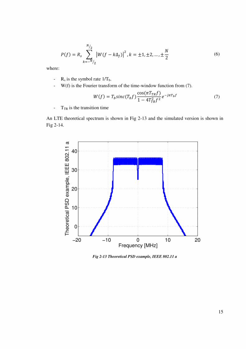
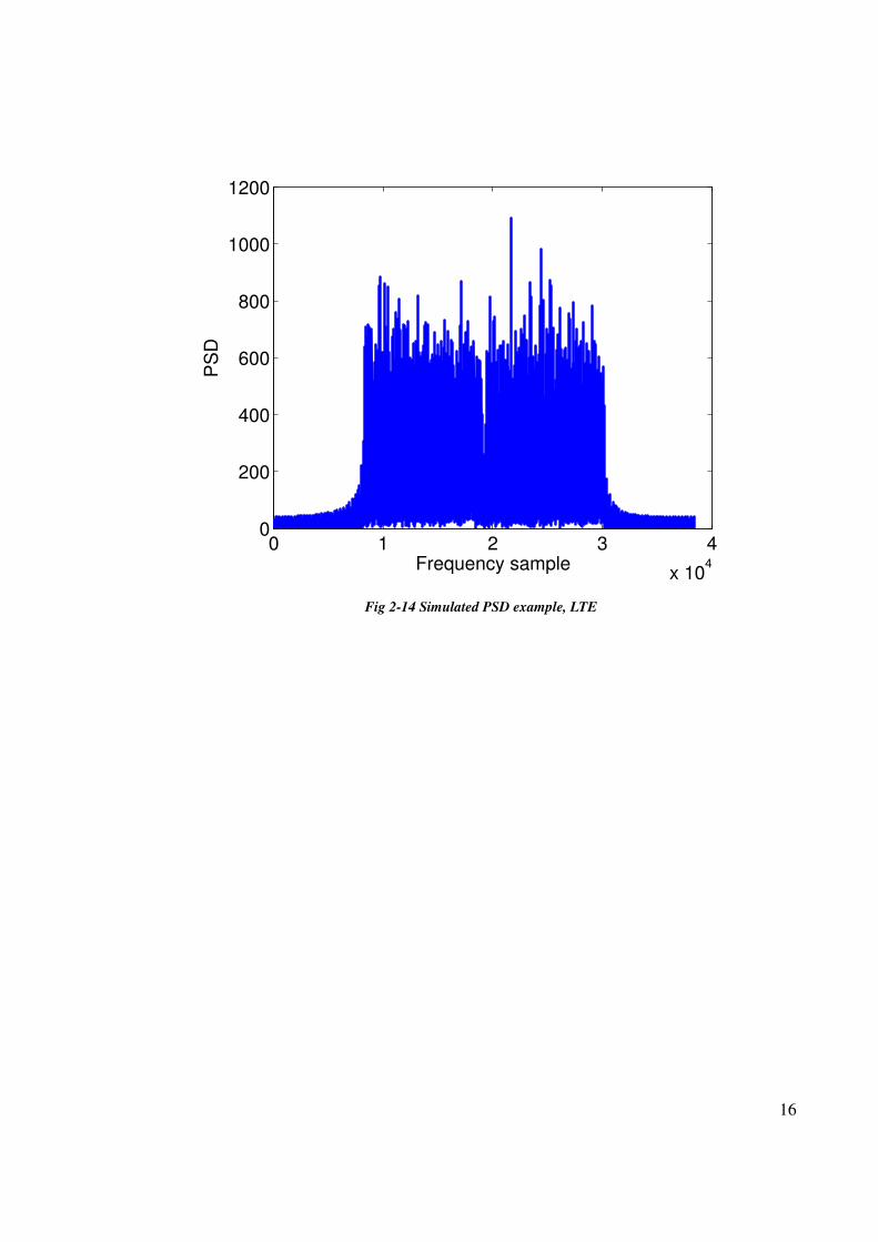
An LTE theoretical spectrum is shown in Fig 2-13 and the simulated version is shown in

Fig 2-14.

Fig 2-13 Theoretical PSD example, IEEE 802.11 a

−20 −10 0 10 20

0

10

20

30

40

Th

eo

retica

l P

SD

exa

mp

le,

IEE

E 8

02

.11

a

Frequency [MHz]

16

Fig 2-14 Simulated PSD example, LTE

0 1 2 3 4

x 104

0

200

400

600

800

1000

1200

Frequency sample

PS

D

17

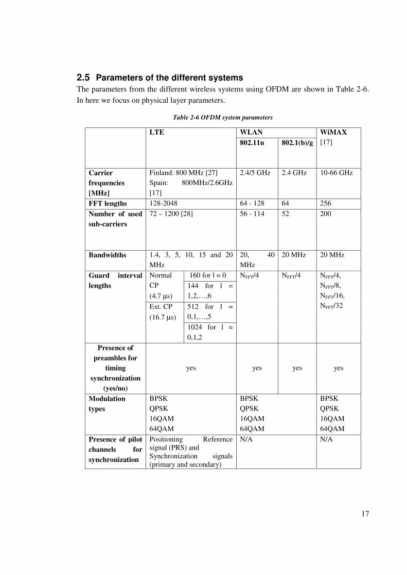
2.5 Parameters of the different systems

The parameters from the different wireless systems using OFDM are shown in Table 2-6.

In here we focus on physical layer parameters.

Table 2-6 OFDM system parameters

LTE WLAN WiMAX

[17] 802.11n

802.1(b)/g

Carrier

frequencies

[MHz]

Finland: 800 MHz [27]

Spain: 800MHz/2.6GHz

[17]

2.4/5 GHz 2.4 GHz 10-66 GHz

FFT lengths 128-2048 64 - 128 64 256

Number of used

sub-carriers

72 – 1200 [28] 56 - 114 52 200

Bandwidths 1.4, 3, 5, 10, 15 and 20

MHz

20, 40

MHz

20 MHz 20 MHz

Guard interval

lengths

Normal

CP

(4.7 µs)

160 for l = 0 NFFT/4 NFFT/4 NFFT/4,

NFFT/8,

NFFT/16,

NFFT/32

144 for l =

1,2,…,6

Ext. CP

(16.7 µs)

512 for l =

0,1,…,5

1024 for l =

0,1,2

Presence of

preambles for

timing

synchronization

(yes/no)

yes yes yes yes

Modulation

types

BPSK

QPSK

16QAM

64QAM

BPSK

QPSK

16QAM

64QAM

BPSK

QPSK

16QAM

64QAM

Presence of pilot

channels for

synchronization

Positioning Reference

signal (PRS) and

Synchronization signals

(primary and secondary)

N/A N/A

18

3 Location principles

In this chapter we give a brief overview of the main localization principles.

Firstly, we define two-dimensional mobile position at time t as eq. (8), and the i-th BS

(or access point or wireless transmitter) position as eq. (9)

�� = �w�, x��t (8)

�� = �w�, x��t (9)

Secondly, we describe the main existing location principles, being ��� a generic time

measurement relative to reference point i and �� the uncertainty due to the environment

[29]. All measured times have to be multiplied by the speed of light to get the measure in

meters.

3.1 Received Signal Strength (RSS)

Positioning systems that make use of received signal strength based location techniques

have been studied for supporting location based services both in indoor and outdoor areas.

Before estimating the mobile position, we need a data collection or training phase, where

location fingerprints are gathered. A location fingerprint consists of a vector R of the

average RSS values from multiple Access Points (APs) at a particular location. In this case,

both the receiver and the emitter know the system power value [29]. As a result, the

channel attenuation can be calculated by measuring the received power, and distance

estimation can be done due to the fact that attenuation increases with distance. Many path-

loss models exist in the literature, such as: simplified path loss model [30], floor and wall

path loss models [31] Okumura-Hata model [32], and so on.

For example, Okumura-Hata model from eq. (10) may be employed. Notice that �� has

values in the range from 4 dB to 12 dB depending on the environment, ��� is a generic time

measurement in dB relative to reference point i, and K and α are parameters [33].

��� = y − 10z log*,/o�� − ��o0 +�� (10)

Where:

- K = 69.55 + 26.16 log*,� ̀ � − 13.82 log*,�ℎ�� − ��ℎ�� - α = �44.9 − 6.55log*,�ℎ���/10

19

- fc is the system carrier frequency

- hb is the BS effective antenna height

- hm is the MS antenna height

- a(hm) is the correction factor for hm

After measuring RSS vector, the Euclidean signal distance between measured data and

previously made fingerprint is calculated [34].

The RSS-based estimation is out of scope of this thesis.

3.2 Time Of Arrival (TOA)

The disadvantage of the RSS method is the random deviation from mean received signal

strength caused by shadowing and small scale channel effect [35]. As a consequence, TOA

of the direct path of the signal could offer higher accuracy in mobile location techniques.

Nevertheless, such techniques are highly dependent on the system parameters, such as

multiple access technique and modulation technique and cannot be used in a generic way.

The TOA location principle consists of calculating the travel time of the signal in a

synchronized network [29], and after that time can be converted to distance by knowing

the propagation speed. Unfortunately, the MS clock is not synchronized and its effect can

be treated as a noise parameter. The performance of the measurement from eq. (11), where ��� is a generic time measurement in meters relative to reference point i and �� is the

uncertainty of the measure, depends on the synchronization accuracy.

��� =o�� − ��o +�� (11)

3.3 Time Difference Of Arrival (TDOA)

When the transmitters are not synchronized, an improvement to TOA measurement

consists of taking time differences of measurements as eq. (12) shows, where ��� is a

generic time measurement in meters relative to reference point i and �� is the uncertainty of

the measure. As a result, the measurement is related to relative distance and the clock bias

nuisance parameter is eliminated [29]. Despite of it is not necessary to report neither

synchronization parameters nor the reference point to the mobile station with this location

principle, synchronization accuracy and base station position determine the system

performance.

���,L =o�� − ��o − o�� − �Lo + �� − �L (12)

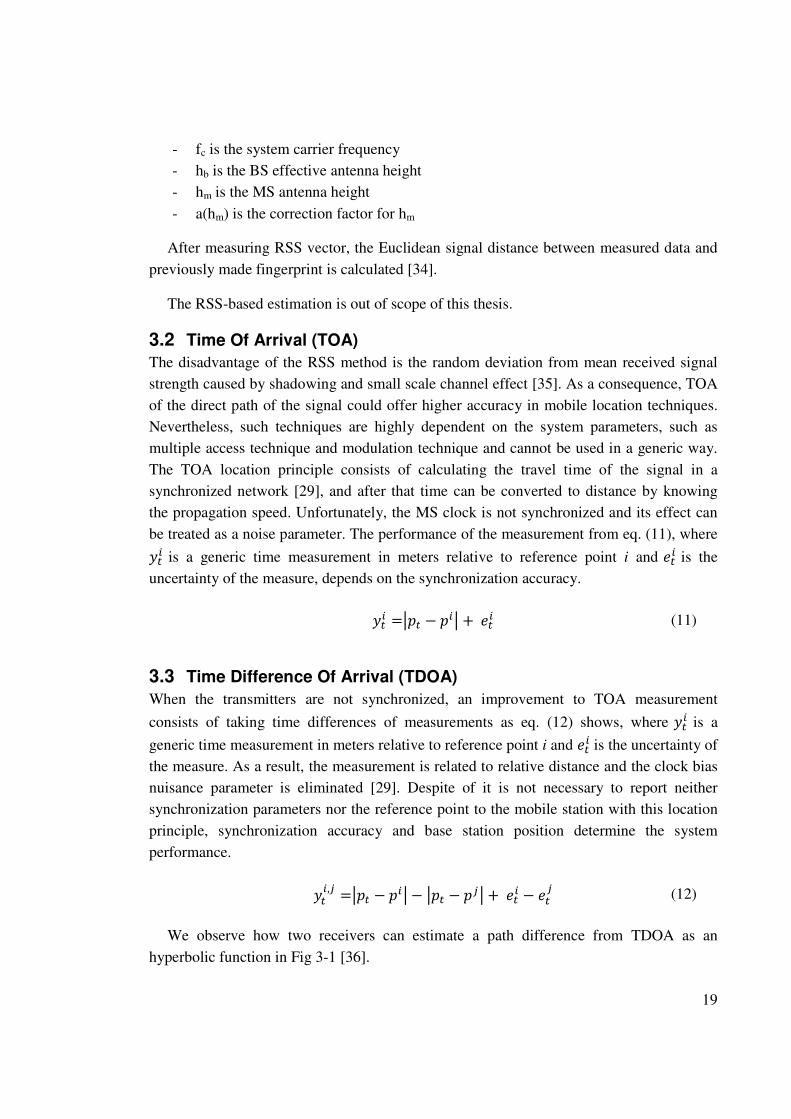
We observe how two receivers can estimate a path difference from TDOA as an

hyperbolic function in Fig 3-1 [36].

20

Fig 3-1 Hyperbolic function representing constant TDOA for three different TDOA's [36]

Basically, the algorithms presented in this thesis are applicable to TOA and TDOA

estimators. However, the TOA/TDOA part has not been explicitly addressed in here, since

we focused on single link (transmitter-receiver) estimation.

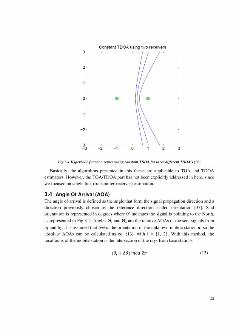
3.4 Angle Of Arrival (AOA)

The angle of arrival is defined as the angle that form the signal propagation direction and a

direction previously chosen as the reference direction, called orientation [37]. Said

orientation is represented in degrees where 0º indicates the signal is pointing to the North,

as represented in Fig 3-2. Angles Θ1 and Θ2 are the relative AOAs of the sent signals from

b1 and b2. It is assumed that ∆Θ is the orientation of the unknown mobile station u, so the

absolute AOAs can be calculated as eq. (13), with i = {1, 2}. With this method, the

location is of the mobile station is the intersection of the rays from base stations.

���+∆�����2% (13)

21

Fig 3-2 Mobile localization with AOA and orientation information [37]

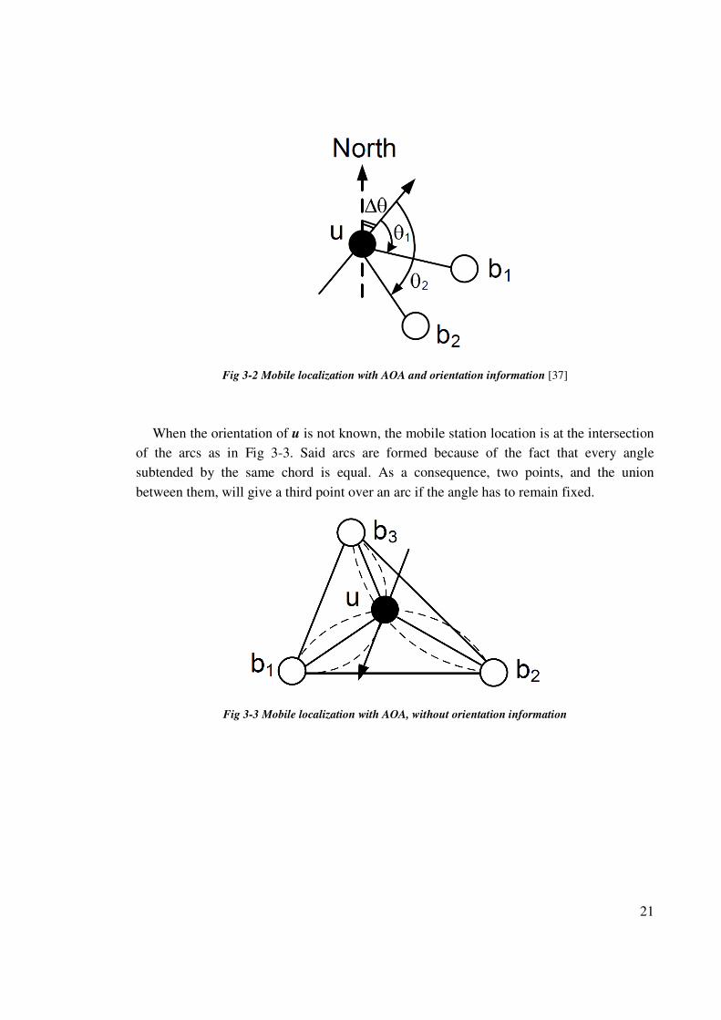
When the orientation of u is not known, the mobile station location is at the intersection

of the arcs as in Fig 3-3. Said arcs are formed because of the fact that every angle

subtended by the same chord is equal. As a consequence, two points, and the union

between them, will give a third point over an arc if the angle has to remain fixed.

Fig 3-3 Mobile localization with AOA, without orientation information

22

4 Timing estimation with OFDM

In this chapter, the different algorithms under study in this thesis are explained. Timing

estimation wants to reach symbol synchronization by finding the starting point of the

OFDM symbol, i.e. the position of the Discrete Fourier Transform (DFT) window [38].

We focus on correlation based estimators with different preamble structures, and a high

resolution algorithm. Note that N is the number of sub-carriers.

4.1 Correlation-based timing synchronization

The basic Correlation-Based Timing Synchronization (CBTS) method consists of

calculating the correlation between the received signal and a known reference replica (e.g.

based on pilot sequences) at the receiver as in eq. (14), where x(k) is the k-th sample of a

known emitted sequence and r(k) is the k-th sample of the received signal [38]. After that,

the estimation is done by finding the sample where the correlation has a maximum.

R�d�= ��r�d-k�x�k�N-1k=0 � (14)

4.2 Preamble-based

Another type of CBTS estimator does the autocorrelation between the received signal and

conjugation of delayed received signal as eq. (15) shows, in which constant delay D is

selected as integral times of sequence.

R�d�= ��r�d-k�r∗�d-k-D�N-1k=0 � (15)

The algorithm from eq. (15) can ensure better performance because phase information

suffers from high variations under bad channel conditions, so two adjacent symbols are

affected almost equally and they still have high correlation [38]. For this reason, we

proceed to present different algorithms that work with some variations on eq. (15), by

introducing different preamble structures and taking profit of their correlation properties.

4.2.1 Schmidl preamble

This method consists of a low-complexity algorithm that allows acquiring synchronization

for both a continuous stream of data and for bursts of data. The symbol timing

synchronization depends on finding a training symbol, usually called preamble. In Schmidl

algorithm, the said preamble consists of two identical halves made by transmitting a

23

pseudo noise (PN) sequence on the even frequencies and zeros on the odd frequencies. For

this reason, the time domain preamble in (16) cannot be mistaken as data frames, which

use every frequency [10]. The generation of the preamble can be also done by using an

IFFT of N/2 sample length over a PN sequence of N sample length.

]<�����`����� = ��( Ur �( Ur � (16)

Considering that the first part of the preamble is identical to the second one except for a

phase shift, the channel effect should be cancelled by multiplying the conjugate of one

sample of the first preamble part with the corresponding sample from the second preamble

part, as eq. (17) shows.

PSchmidl�d�=∑ r*�d+k�r "d+k+ N2'N2-1k=0 (17)

where r is the received signal and d is a time index corresponding to the first simple in a

window of length N. The received energy is defined in eq. (18) and allows us to use the

timing metric defined in eq. (19), whose maximum reveals the preamble start.

ESchmidl�d�=��r �d+k+N2��2N2-1

k=0 (18)

MSchmidl�d�= |PSchmidl�d�|2�ESchmidl�d��2 (19)

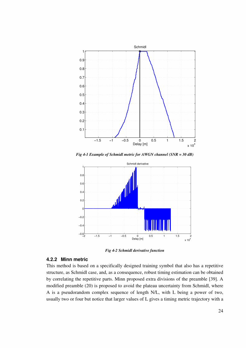
As Fig 4-1 shows, the timing metric MSchmidl for an OFDM signal with 1024 sub-carriers

over an AWGN channel with a Signal-to-Noise Ratio (SNR) of 30dB has a flat region with

a length equal to the guard interval minus the length of the channel impulse response.

Although said flat region makes it difficult to find the exact position of the maximum, it is

located at the beginning of the flat region and can be found by calculating where the

derivative of the metric has its first zero as shown in Fig 4-2.

24

Fig 4-1 Example of Schmidl metric for AWGN channel (SNR = 30 dB)

Fig 4-2 Schmidl derivative function

4.2.2 Minn metric

This method is based on a specifically designed training symbol that also has a repetitive

structure, as Schmidl case, and, as a consequence, robust timing estimation can be obtained

by correlating the repetitive parts. Minn proposed extra divisions of the preamble [39]. A

modified preamble (20) is proposed to avoid the plateau uncertainty from Schmidl, where

A is a pseudorandom complex sequence of length N/L, with L being a power of two,

usually two or four but notice that larger values of L gives a timing metric trajectory with a

−1.5 −1 −0.5 0 0.5 1 1.5 2

x 104

0.1

0.2

0.3

0.4

0.5

0.6

0.7

0.8

0.9

1

Delay [m]

Schmidl

−2 −1.5 −1 −0.5 0 0.5 1 1.5 2

x 104

−0.6

−0.4

−0.2

0

0.2

0.4

0.6

0.8

1

Delay [m]

Schmidl derivative

25

steeper roll off [39]. The signs of each part are designed to achieve the sharpest timing

metric.

Preambleh����=�±AN Lr ±AN Lr ±AN Lr …±AN Lr � (20)

A new metric (21) is used in this method, where L is the number of preamble parts and

each preamble part contains M samples. Moreover, the metric elements definition changes

slightly in (22) and (23) compared to Schmidl metric.

where MMinn�d�= � LL-1�2 |Ph����d�|2�EMinn�d��2 (21)

PMinn�d� = � ���� � r*�d+m·M+k�·h)*

k=0L-2m=0

r�d+�m+1�M+k� (22)

EMinn�d�=��|r�d+k+m·M�|2�-1

m=0

M-1k=0

(23)

and b(m) is p(m)·p(m+1), where p(m) denotes the sign of the repeated parts of the training

symbol.

One of the Minn’s preamble structures, balanced between complexity and accuracy, is

defined in eq. (24), with L being four and M being N/4 [11]. As a result, MMinn, PMinn and

EMinn are simplified in eq. (25), eq. (26) and eq. (27), respectively. This was the choice of

our implementation as well.

Preambleh����= �AN �r AN �r -AN �r -AN 4r � (24)

MMinn�d�= �43�2 |Ph����d�|2�EMinn�d��2 (25)

PMinn�d� = � � r* �d+m·

�4 +k� ·

(/�)*k=0

Um=0

r �d+�m+1�· �4 +k�

(26)

26

EMinn�d�= � ��r �d+k+m·�4��

23m=0

N/4-1k=0

(27)

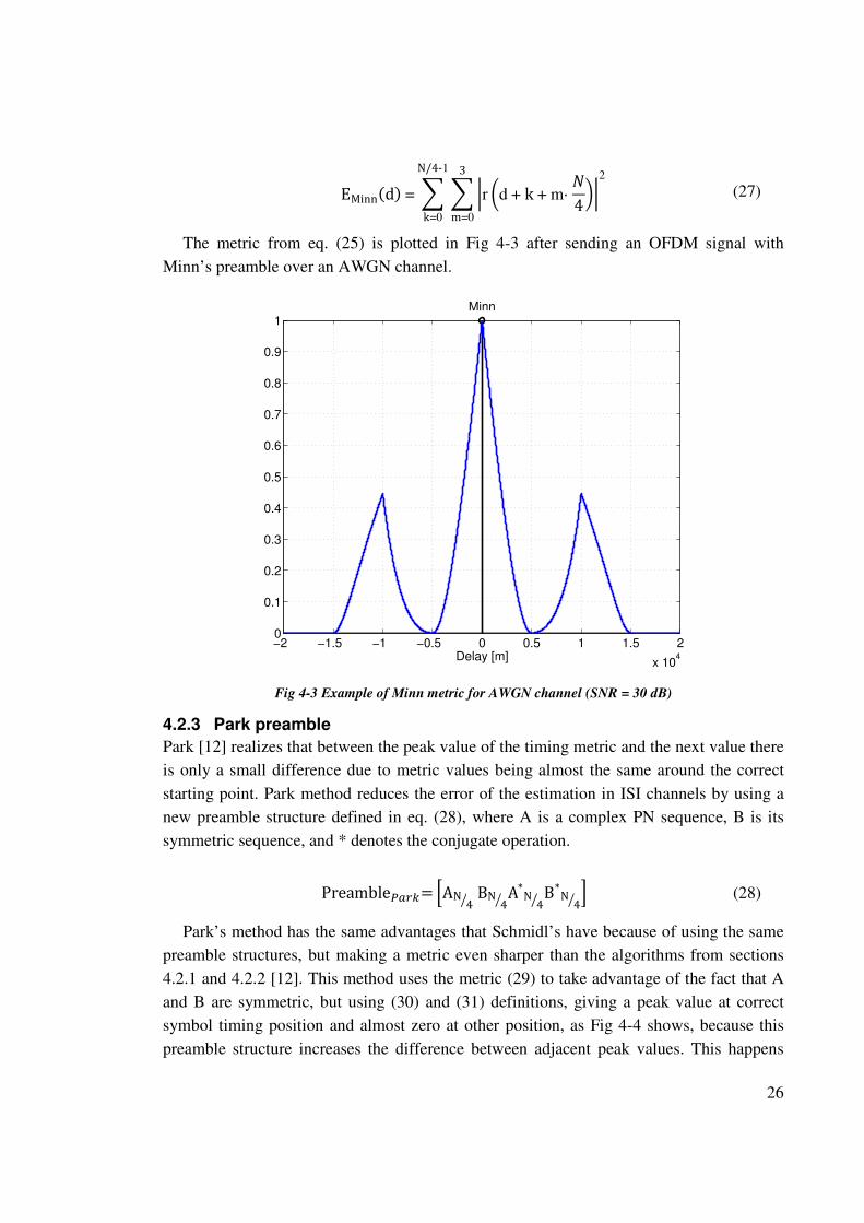
The metric from eq. (25) is plotted in Fig 4-3 after sending an OFDM signal with

Minn’s preamble over an AWGN channel.

Fig 4-3 Example of Minn metric for AWGN channel (SNR = 30 dB)

4.2.3 Park preamble

Park [12] realizes that between the peak value of the timing metric and the next value there

is only a small difference due to metric values being almost the same around the correct

starting point. Park method reduces the error of the estimation in ISI channels by using a

new preamble structure defined in eq. (28), where A is a complex PN sequence, B is its

symmetric sequence, and * denotes the conjugate operation.

Preamblee� �= �AN 4r BN 4r A*N 4r B*N 4r � (28)

Park’s method has the same advantages that Schmidl’s have because of using the same

preamble structures, but making a metric even sharper than the algorithms from sections

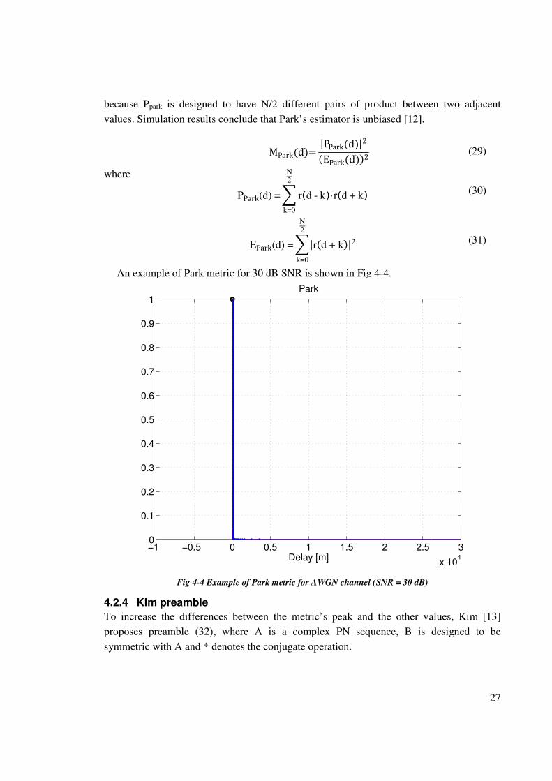
4.2.1 and 4.2.2 [12]. This method uses the metric (29) to take advantage of the fact that A

and B are symmetric, but using (30) and (31) definitions, giving a peak value at correct

symbol timing position and almost zero at other position, as Fig 4-4 shows, because this

preamble structure increases the difference between adjacent peak values. This happens

−2 −1.5 −1 −0.5 0 0.5 1 1.5 2

x 104

0

0.1

0.2

0.3

0.4

0.5

0.6

0.7

0.8

0.9

1

Delay [m]

Minn

27

because Ppark is designed to have N/2 different pairs of product between two adjacent

values. Simulation results conclude that Park’s estimator is unbiased [12].

MPark�d�= |PPark�d�|2�EPark�d��2 (29)

where

PPark(d)=� r�d-k�·r�d+k�N2

k=0

(30)

EPark(d) =�|r�d + k�|2N2

k=0

(31)

An example of Park metric for 30 dB SNR is shown in Fig 4-4.

Fig 4-4 Example of Park metric for AWGN channel (SNR = 30 dB)

4.2.4 Kim preamble

To increase the differences between the metric’s peak and the other values, Kim [13]

proposes preamble (32), where A is a complex PN sequence, B is designed to be

symmetric with A and * denotes the conjugate operation.

−1 −0.5 0 0.5 1 1.5 2 2.5 3

x 104

0

0.1

0.2

0.3

0.4

0.5

0.6

0.7

0.8

0.9

1

Delay [m]

Park

28

]<����¢��= �AN 4r B*N 4r AN 4r B*N 4r � (32)

The metric is (33) in this case, and it is designed taking into account the fact that B* is

symmetric and conjugate with A.

M¢���d�= |PKim�d�|2�EKim�d��2 (33)

where PKim(d)=� r �d–k+N

2� r �d+k+N

2�

N2

-1

k=0

(34)

and

EKim�d�=��r �d+k+N2��2

N2-1

k=0

(35)

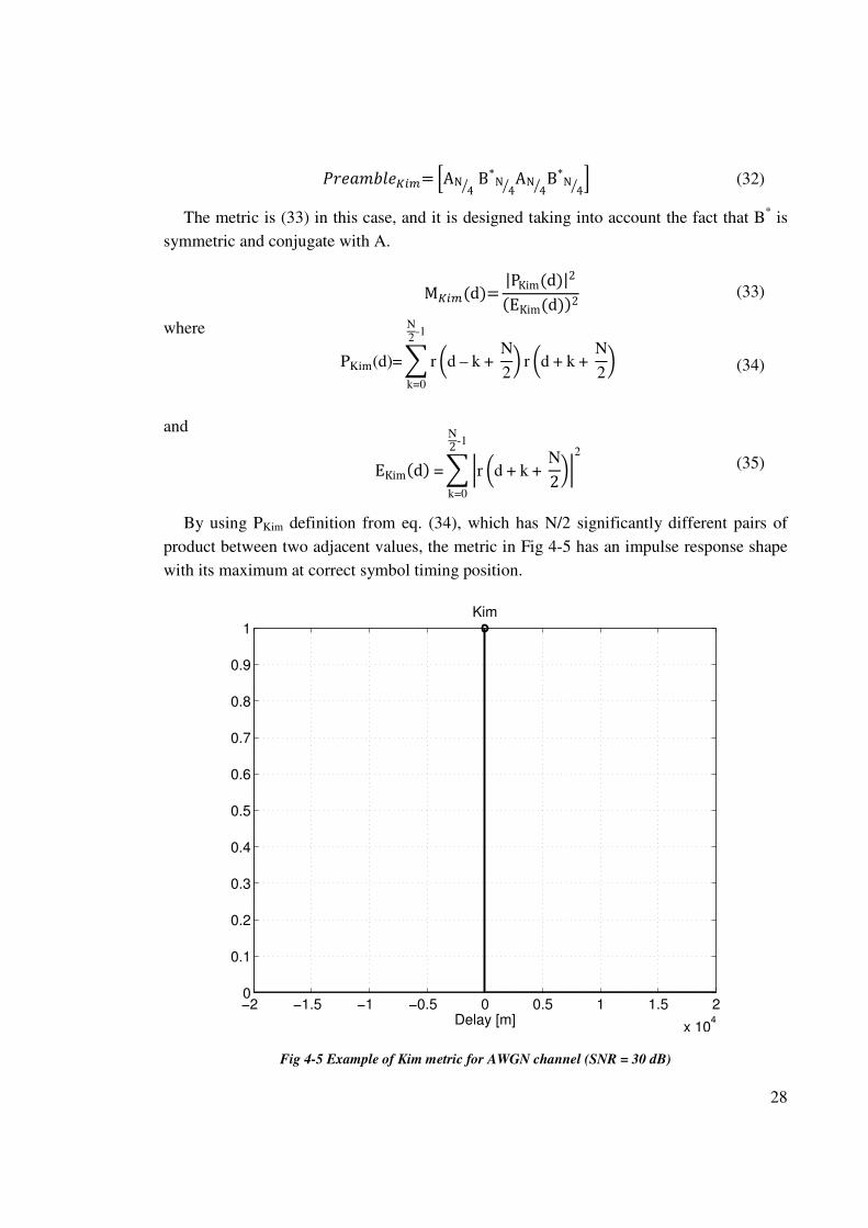
By using PKim definition from eq. (34), which has N/2 significantly different pairs of

product between two adjacent values, the metric in Fig 4-5 has an impulse response shape

with its maximum at correct symbol timing position.

Fig 4-5 Example of Kim metric for AWGN channel (SNR = 30 dB)

−2 −1.5 −1 −0.5 0 0.5 1 1.5 2

x 104

0

0.1

0.2

0.3

0.4

0.5

0.6

0.7

0.8

0.9

1

Delay [m]

Kim

29

4.2.5 Ren preamble

A new preamble (36) is defined to enlarge the difference between consecutive positions of

the metric from eq. (37) [14]. This method uses a constant envelop preamble which

consists of two Constant Amplitude Zero Auto-Correlation (CAZAC) sequences, of length

N/2, multiplied with the Hadamard product by a real PN sequence of length N, whose

values are +1 or -1. The real PN sequence is used to take advantage of the constant envelop

preamble because it increases the difference MRen(d) – MRen(d+1) . The operator o

indicates the Hadamard product, which is defined as element by element multiplications of

two vectors.

]<����u¤�= �CN 2r CN 2r � oSN (36)

The working definitions for this method are given by (38) and (39), where sk is the k-th

element of SN.

Mu¤��d�= |PKim�d�|2�EKim�d��2 (37)

PRen(d)=� sksk+N

2r · r*�d + k�·r �d + k + N

2�

N2

-1

k=0

(38)

ERen�d� = 1

2�|r�d + k �|2N2

-1

k=0

(39)

The metric in Fig 4-6, which is based on finding the highest correlation between two

repeated sequences, has its peak at correct symbol timing position and much smaller values

at incorrect positions due to the correlation property of SN weighted factors. Ren’s metric

is robust to frequency offset as reported in [14].

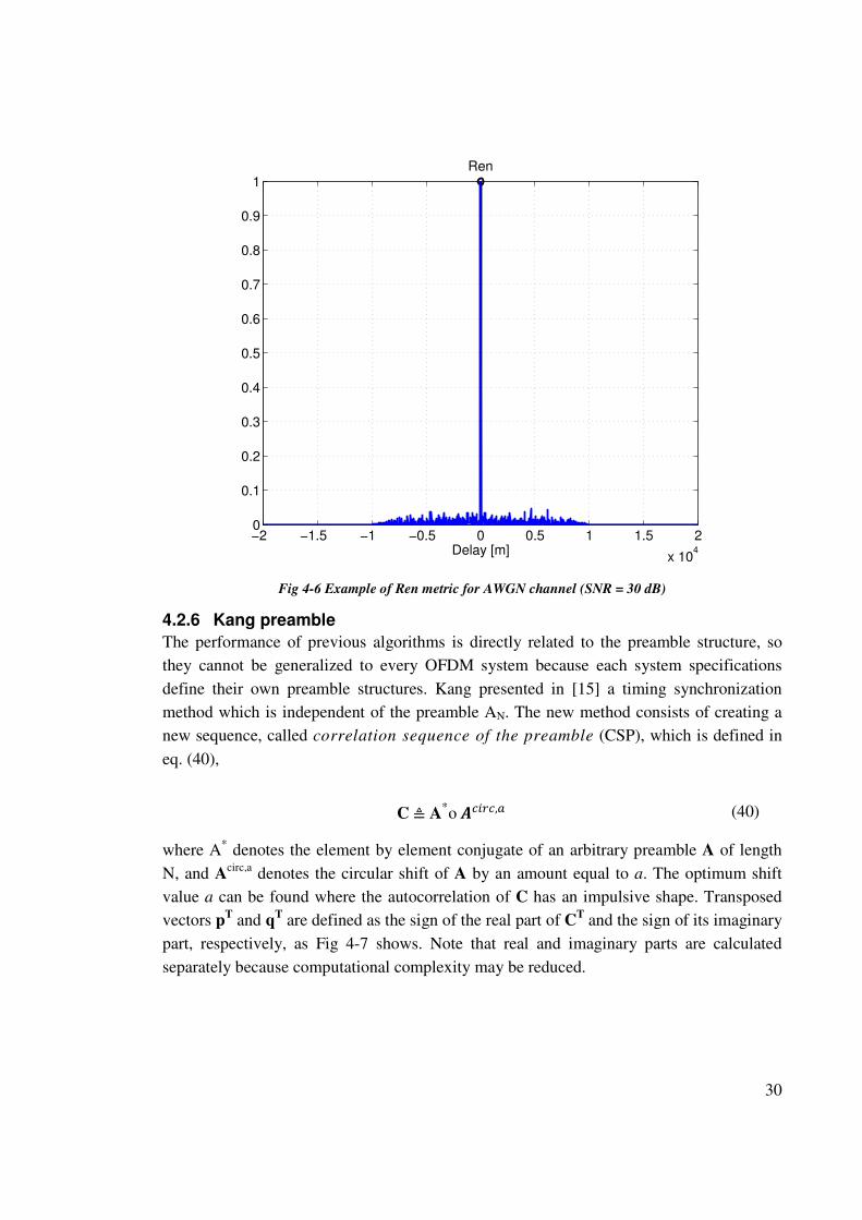
30

Fig 4-6 Example of Ren metric for AWGN channel (SNR = 30 dB)

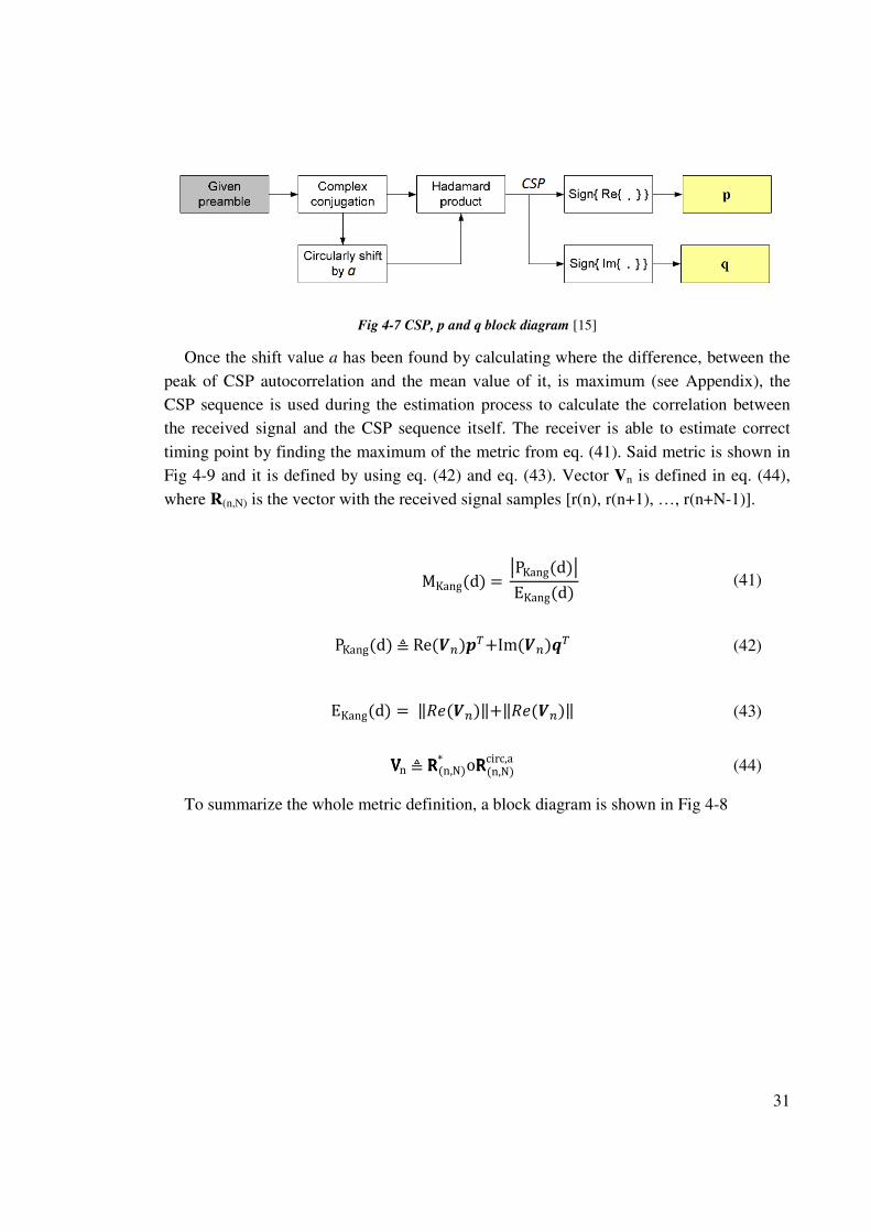
4.2.6 Kang preamble

The performance of previous algorithms is directly related to the preamble structure, so

they cannot be generalized to every OFDM system because each system specifications

define their own preamble structures. Kang presented in [15] a timing synchronization

method which is independent of the preamble AN. The new method consists of creating a

new sequence, called correlation sequence of the preamble (CSP), which is defined in

eq. (40),

C≜ A*o§`� `,� (40)

where A* denotes the element by element conjugate of an arbitrary preamble A of length

N, and Acirc,a

denotes the circular shift of A by an amount equal to a. The optimum shift

value a can be found where the autocorrelation of C has an impulsive shape. Transposed

vectors pT and qT are defined as the sign of the real part of CT and the sign of its imaginary

part, respectively, as Fig 4-7 shows. Note that real and imaginary parts are calculated

separately because computational complexity may be reduced.

−2 −1.5 −1 −0.5 0 0.5 1 1.5 2

x 104

0

0.1

0.2

0.3

0.4

0.5

0.6

0.7

0.8

0.9

1

Delay [m]

Ren

31

Fig 4-7 CSP, p and q block diagram [15]

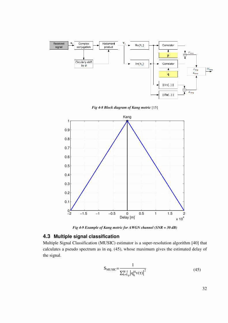
Once the shift value a has been found by calculating where the difference, between the

peak of CSP autocorrelation and the mean value of it, is maximum (see Appendix), the

CSP sequence is used during the estimation process to calculate the correlation between

the received signal and the CSP sequence itself. The receiver is able to estimate correct

timing point by finding the maximum of the metric from eq. (41). Said metric is shown in

Fig 4-9 and it is defined by using eq. (42) and eq. (43). Vector Vn is defined in eq. (44),

where R(n,N) is the vector with the received signal samples [r(n), r(n+1), …, r(n+N-1)].

To summarize the whole metric definition, a block diagram is shown in Fig 4-8

MKang�d�= oPKang�d�oEKang�d� (41)

PKang�d�≜Re�¨��©t+Im�¨��«t (42)

EKang�d� = ‖n�¨��‖+‖n�¨��‖ (43)

VVVVn≜RRRR�n,N�* oRRRR�n,N�circ,a (44)

32

Fig 4-8 Block diagram of Kang metric [15]

Fig 4-9 Example of Kang metric for AWGN channel (SNR = 30 dB)

4.3 Multiple signal classification

Multiple Signal Classification (MUSIC) estimator is a super-resolution algorithm [40] that

calculates a pseudo spectrum as in eq. (45), whose maximum gives the estimated delay of

the signal.

SMUSIC=1∑ oqkHv(τ)o2(-1

k=Lp

(45)

−2 −1.5 −1 −0.5 0 0.5 1 1.5 2

x 104

0

0.1

0.2

0.3

0.4

0.5

0.6

0.7

0.8

0.9

1

Delay [m]

Kang

33

where Lp is the number of estimated multipath components from the channel model, N

denotes the total number of equally spaced frequencies, qk is the k-th noise eigenvector

(eigenvectors corresponding to N-Lp smallest eigenvalues) of the covariance matrix of the

received signal, the upper index H denotes the Hermitian operation, and v(τk) is defined by

(46), where super index T denotes transpose operation and ∆f is the separation between

sub-carriers.

v�τk�=l1e-j2π∆fτk…e-j2π(N-1)∆fτkmT (46)

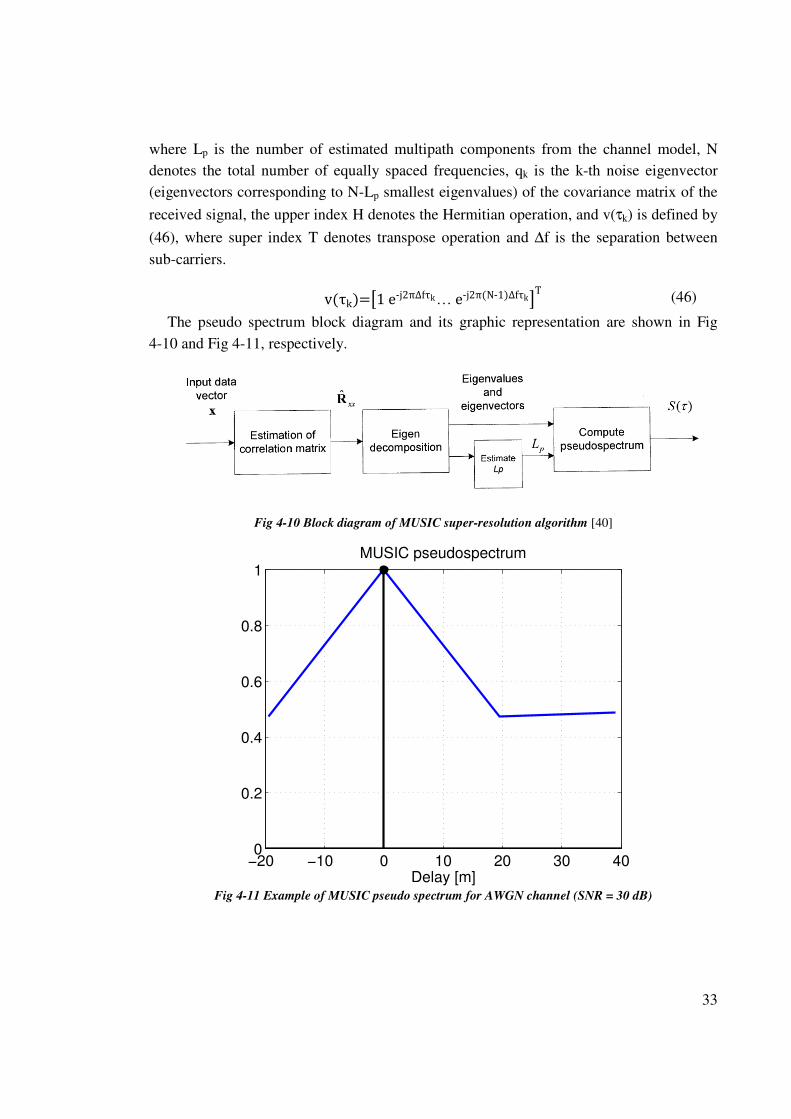
The pseudo spectrum block diagram and its graphic representation are shown in Fig

4-10 and Fig 4-11, respectively.

Fig 4-10 Block diagram of MUSIC super-resolution algorithm [40]

Fig 4-11 Example of MUSIC pseudo spectrum for AWGN channel (SNR = 30 dB)

−20 −10 0 10 20 30 400

0.2

0.4

0.6

0.8

1MUSIC pseudospectrum

Delay [m]

34

5 Simulation model

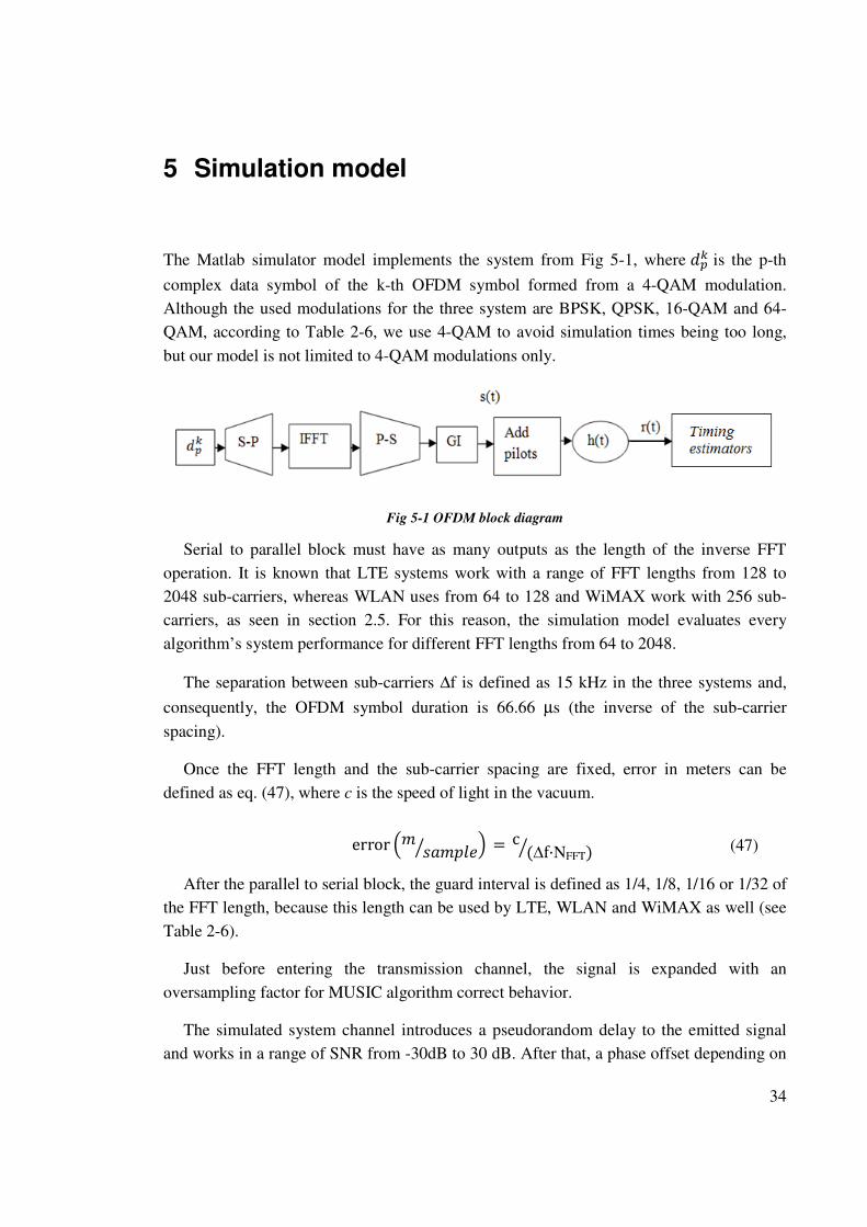
The Matlab simulator model implements the system from Fig 5-1, where ��� is the p-th

complex data symbol of the k-th OFDM symbol formed from a 4-QAM modulation.

Although the used modulations for the three system are BPSK, QPSK, 16-QAM and 64-

QAM, according to Table 2-6, we use 4-QAM to avoid simulation times being too long,

but our model is not limited to 4-QAM modulations only.

Fig 5-1 OFDM block diagram

Serial to parallel block must have as many outputs as the length of the inverse FFT

operation. It is known that LTE systems work with a range of FFT lengths from 128 to

2048 sub-carriers, whereas WLAN uses from 64 to 128 and WiMAX work with 256 sub-

carriers, as seen in section 2.5. For this reason, the simulation model evaluates every

algorithm’s system performance for different FFT lengths from 64 to 2048.

The separation between sub-carriers ∆f is defined as 15 kHz in the three systems and,

consequently, the OFDM symbol duration is 66.66 µs (the inverse of the sub-carrier

spacing).

Once the FFT length and the sub-carrier spacing are fixed, error in meters can be

defined as eq. (47), where c is the speed of light in the vacuum.

error "� �����r ' = c (∆f·NFFT)r (47)

After the parallel to serial block, the guard interval is defined as 1/4, 1/8, 1/16 or 1/32 of

the FFT length, because this length can be used by LTE, WLAN and WiMAX as well (see

Table 2-6).

Just before entering the transmission channel, the signal is expanded with an

oversampling factor for MUSIC algorithm correct behavior.

The simulated system channel introduces a pseudorandom delay to the emitted signal

and works in a range of SNR from -30dB to 30 dB. After that, a phase offset depending on

35

the frequency offset is added to the delayed signal. Finally, the received signal r(t) is

generated by adding AWGN. The simulation model includes a multipath channel with

Rayleigh fading to work in more realistic conditions.

The last step from Fig 5-1 is the timing estimation, which depends on the different

algorithms from Chapter 4. Every algorithm from Chapter 4 has its own metric

calculations but there are some that are common to all algorithms, such as generating a

vector of delays to compute the Root Mean Square Error (RMSE) from eq. (48), padding

the signal with zeros at the beginning and at the end of the received signal and, finally,

finding the maximum of said metric.

RMSE(m)=error(� sampler )·´���((�4-��4�_���� − 4<¶_����)U) (48)

There are some special cases, Schmidl’s and Kang’s algorithms. In Schmidl’s

algorithm, the first maximum value from the plateau needs to be found by computing

where the derivative of the Schmidl metric becomes zero, and Kang’s algorithm needs to

call a function to determine the correct shift of the correlation sequence of the

preamble (CSP) as a previous step to compute the metric.

Supporting Matlab files used in the modelling have been added in the Appendix.

36

6 Simulation results for timing

The performance of the studied estimators is evaluated by RMSE, using Matlab-based

computer simulations. Following sections evaluate the performance of every metric by

changing some system parameters.

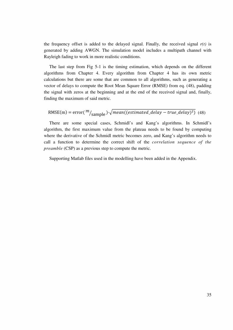
6.1 Comparison for various SNR values

Firstly, the simulator runs with CBTS estimator for different preamble structures to

compare the performance for different SNR in AWGN static single path channel, with

1024 as FFT length, in Fig 6-1. It is observed that CBTS estimator has a similar

performance independently of the preamble structure.

Fig 6-1 CBTS comparison over single path channel

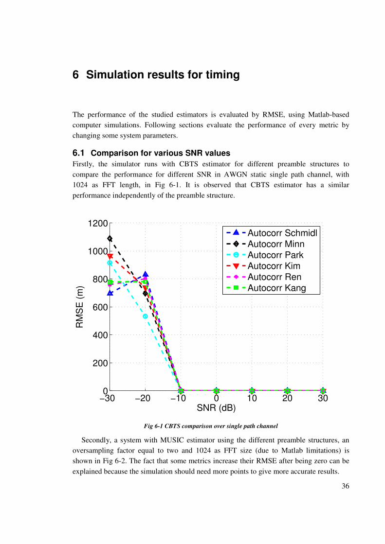
Secondly, a system with MUSIC estimator using the different preamble structures, an

oversampling factor equal to two and 1024 as FFT size (due to Matlab limitations) is

shown in Fig 6-2. The fact that some metrics increase their RMSE after being zero can be

explained because the simulation should need more points to give more accurate results.

−30 −20 −10 0 10 20 300

200

400

600

800

1000

1200

SNR (dB)

RM

SE

(m

)

Autocorr Schmidl

Autocorr Minn

Autocorr ParkAutocorr Kim

Autocorr Ren

Autocorr Kang

37

Fig 6-2 MUSIC comparison over single path channel

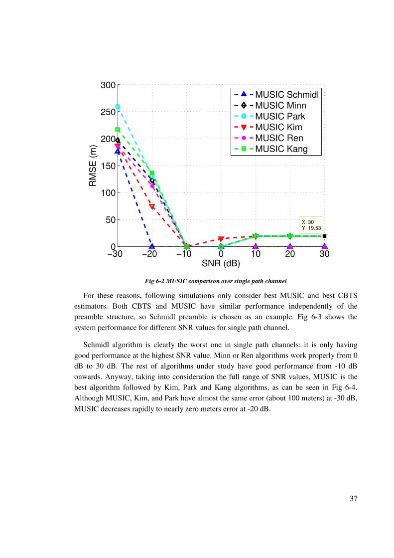
For these reasons, following simulations only consider best MUSIC and best CBTS

estimators. Both CBTS and MUSIC have similar performance independently of the

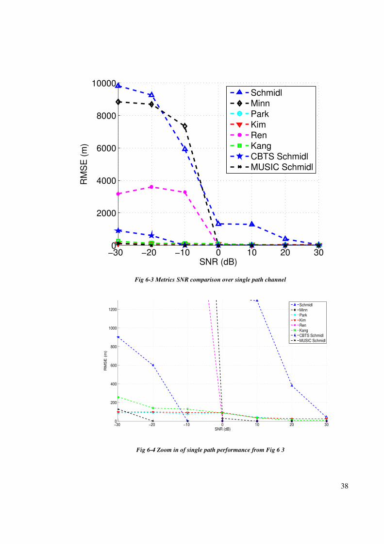
preamble structure, so Schmidl preamble is chosen as an example. Fig 6-3 shows the

system performance for different SNR values for single path channel.

Schmidl algorithm is clearly the worst one in single path channels: it is only having

good performance at the highest SNR value. Minn or Ren algorithms work properly from 0

dB to 30 dB. The rest of algorithms under study have good performance from -10 dB

onwards. Anyway, taking into consideration the full range of SNR values, MUSIC is the

best algorithm followed by Kim, Park and Kang algorithms, as can be seen in Fig 6-4.

Although MUSIC, Kim, and Park have almost the same error (about 100 meters) at -30 dB,

MUSIC decreases rapidly to nearly zero meters error at -20 dB.

−30 −20 −10 0 10 20 300

50

100

150

200

250

300

X: 30Y: 19.53

SNR (dB)

RM

SE

(m

)MUSIC Schmidl

MUSIC Minn

MUSIC ParkMUSIC Kim

MUSIC Ren

MUSIC Kang

38

Fig 6-3 Metrics SNR comparison over single path channel

Fig 6-4 Zoom in of single path performance from Fig 6 3

−30 −20 −10 0 10 20 300

2000

4000

6000

8000

10000

SNR (dB)

RM

SE

(m

)

SchmidlMinn

Park

KimRen

Kang

CBTS SchmidlMUSIC Schmidl

−30 −20 −10 0 10 20 300

200

400

600

800

1000

1200

SNR (dB)

RM

SE

(m

)

SchmidlMinn

Park

KimRen

Kang

CBTS SchmidlMUSIC Schmidl

39

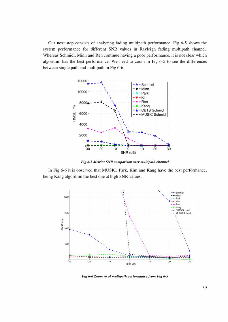
Our next step consists of analyzing fading multipath performance. Fig 6-5 shows the

system performance for different SNR values in Rayleigh fading multipath channel.

Whereas Schmidl, Minn and Ren continue having a poor performance, it is not clear which

algorithm has the best performance. We need to zoom in Fig 6-5 to see the differences

between single path and multipath in Fig 6-6.

Fig 6-5 Metrics SNR comparison over multipath channel

In Fig 6-6 it is observed that MUSIC, Park, Kim and Kang have the best performance,

being Kang algorithm the best one at high SNR values.

Fig 6-6 Zoom in of multipath performance from Fig 6-5

−30 −20 −10 0 10 20 300

2000

4000

6000

8000

10000

12000

SNR (dB)

RM

SE

(m

)

SchmidlMinn

Park

KimRen

Kang

CBTS SchmidlMUSIC Schmidl

−30 −20 −10 0 10 20 300

500

1000

1500

2000

SNR (dB)

RM

SE

(m

)

SchmidlMinn

Park

KimRen

Kang

CBTS SchmidlMUSIC Schmidl

40

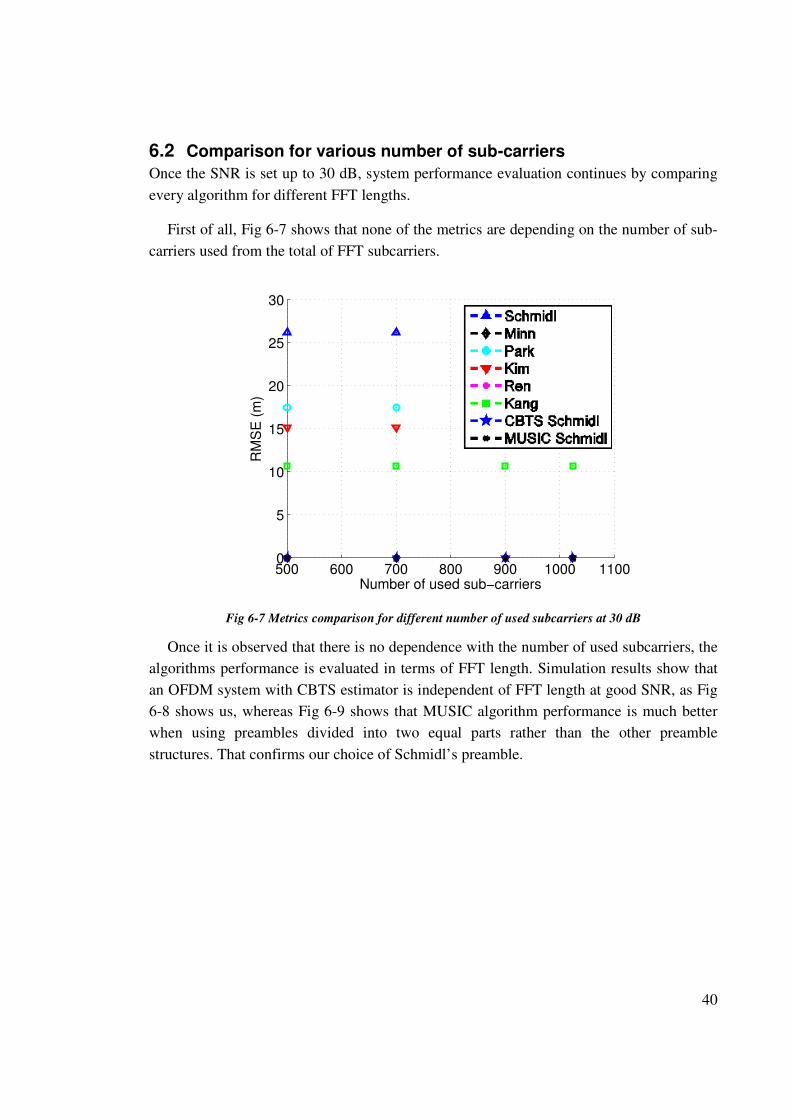
6.2 Comparison for various number of sub-carriers

Once the SNR is set up to 30 dB, system performance evaluation continues by comparing

every algorithm for different FFT lengths.

First of all, Fig 6-7 shows that none of the metrics are depending on the number of sub-

carriers used from the total of FFT subcarriers.

Fig 6-7 Metrics comparison for different number of used subcarriers at 30 dB

Once it is observed that there is no dependence with the number of used subcarriers, the

algorithms performance is evaluated in terms of FFT length. Simulation results show that

an OFDM system with CBTS estimator is independent of FFT length at good SNR, as Fig

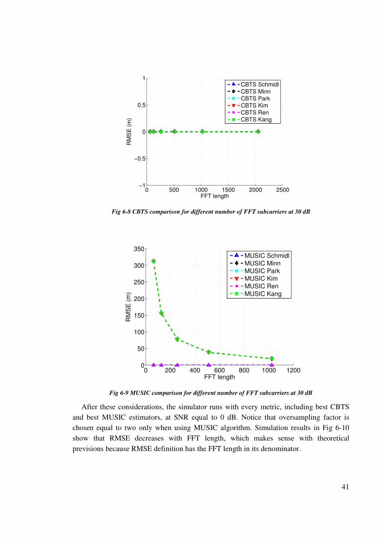
6-8 shows us, whereas Fig 6-9 shows that MUSIC algorithm performance is much better

when using preambles divided into two equal parts rather than the other preamble

structures. That confirms our choice of Schmidl’s preamble.

500 600 700 800 900 1000 11000

5

10

15

20

25

30

Number of used sub−carriers

RM

SE

(m

)

SchmidlMinn

Park

KimRen

Kang

CBTS SchmidlMUSIC Schmidl

41

Fig 6-8 CBTS comparison for different number of FFT subcarriers at 30 dB

Fig 6-9 MUSIC comparison for different number of FFT subcarriers at 30 dB

After these considerations, the simulator runs with every metric, including best CBTS

and best MUSIC estimators, at SNR equal to 0 dB. Notice that oversampling factor is

chosen equal to two only when using MUSIC algorithm. Simulation results in Fig 6-10

show that RMSE decreases with FFT length, which makes sense with theoretical

previsions because RMSE definition has the FFT length in its denominator.

0 500 1000 1500 2000 2500−1

−0.5

0

0.5

1

FFT length

RM

SE

(m

)

CBTS Schmidl

CBTS Minn

CBTS ParkCBTS Kim

CBTS Ren

CBTS Kang

0 200 400 600 800 1000 12000

50

100

150

200

250

300

350

FFT length

RM

SE

(m

)

MUSIC Schmidl

MUSIC Minn

MUSIC ParkMUSIC Kim

MUSIC Ren

MUSIC Kang

42

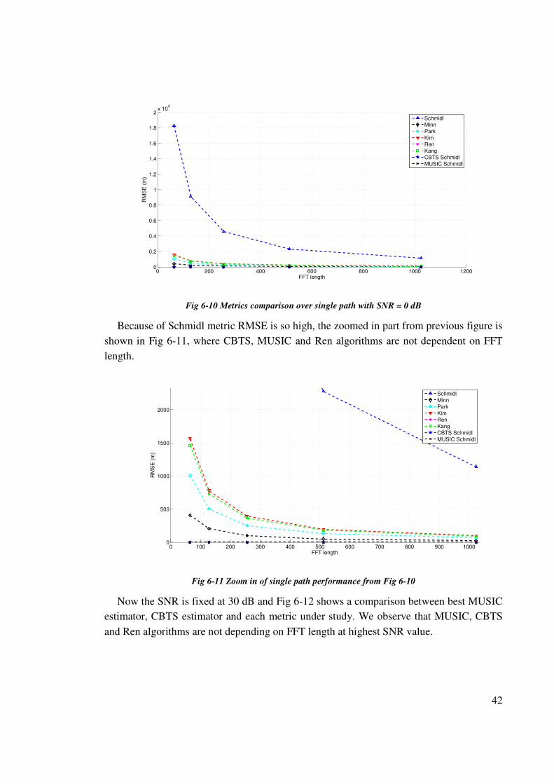
Fig 6-10 Metrics comparison over single path with SNR = 0 dB

Because of Schmidl metric RMSE is so high, the zoomed in part from previous figure is

shown in Fig 6-11, where CBTS, MUSIC and Ren algorithms are not dependent on FFT

length.

Fig 6-11 Zoom in of single path performance from Fig 6-10

Now the SNR is fixed at 30 dB and Fig 6-12 shows a comparison between best MUSIC

estimator, CBTS estimator and each metric under study. We observe that MUSIC, CBTS

and Ren algorithms are not depending on FFT length at highest SNR value.

0 200 400 600 800 1000 12000

0.2

0.4

0.6

0.8

1

1.2

1.4

1.6

1.8

2x 10

4

FFT length

RM

SE

(m

)

SchmidlMinn

Park

KimRen

Kang

CBTS SchmidlMUSIC Schmidl

0 100 200 300 400 500 600 700 800 900 10000

500

1000

1500

2000

FFT length

RM

SE

(m

)

SchmidlMinn

Park

KimRen

Kang

CBTS SchmidlMUSIC Schmidl

43

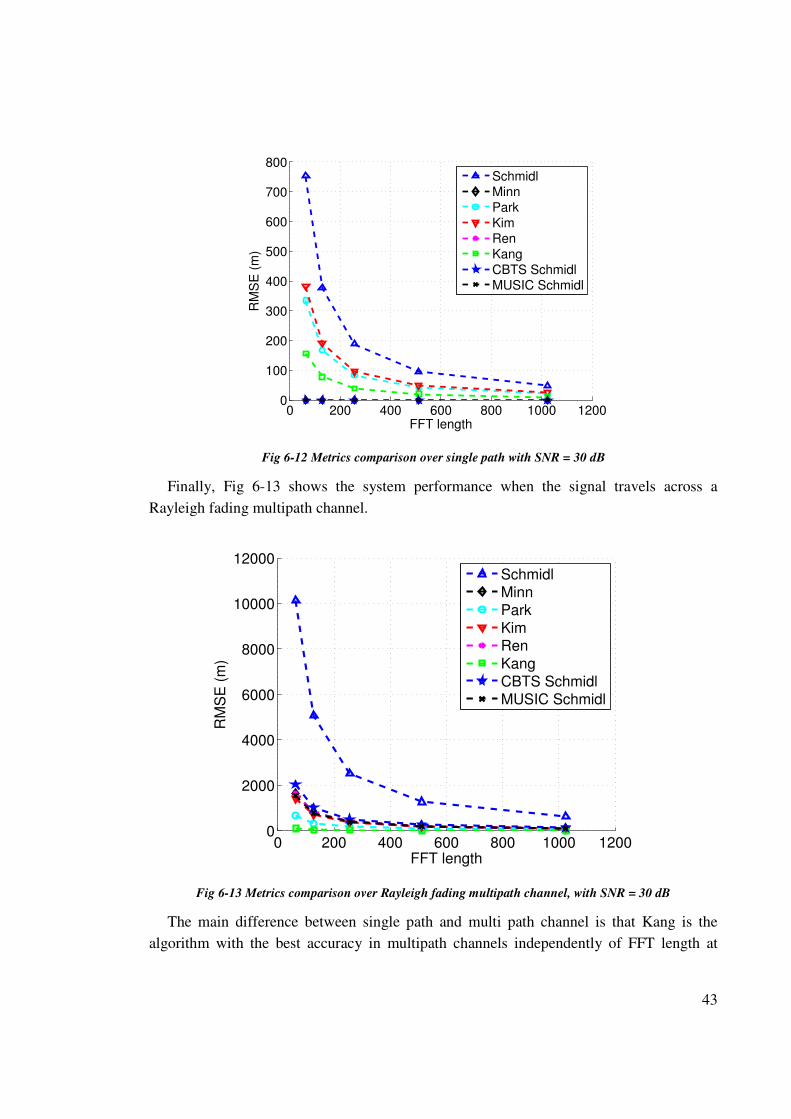
Fig 6-12 Metrics comparison over single path with SNR = 30 dB

Finally, Fig 6-13 shows the system performance when the signal travels across a

Rayleigh fading multipath channel.

Fig 6-13 Metrics comparison over Rayleigh fading multipath channel, with SNR = 30 dB

The main difference between single path and multi path channel is that Kang is the

algorithm with the best accuracy in multipath channels independently of FFT length at

0 200 400 600 800 1000 12000

100

200

300

400

500

600

700

800

FFT length

RM

SE

(m

)

SchmidlMinn

Park

KimRen

Kang

CBTS SchmidlMUSIC Schmidl

0 200 400 600 800 1000 12000

2000

4000

6000

8000

10000

12000

FFT length

RM

SE

(m

)

SchmidlMinn

Park

KimRen

Kang

CBTS SchmidlMUSIC Schmidl

44

good SNR, whereas CBTS, MUSIC and Ren are the best algorithms over single path

channels because the three of them are robust to FFT length.

The FFT length is set to 1024 for the following sections, because the metrics that are

depending on it have better performance with higher number of subcarriers.

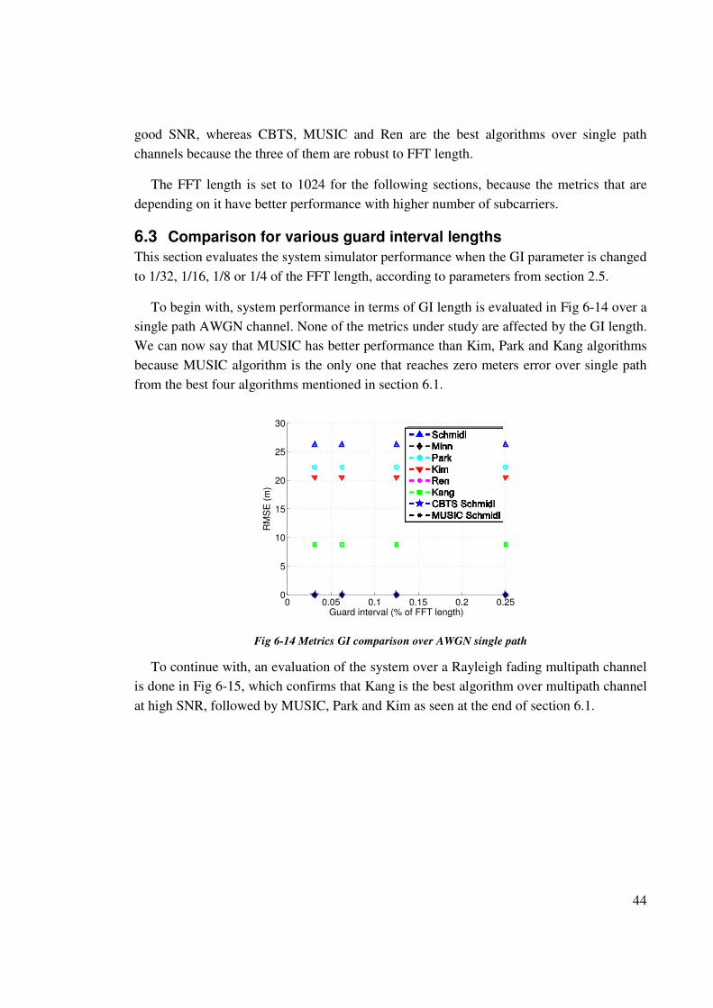
6.3 Comparison for various guard interval lengths

This section evaluates the system simulator performance when the GI parameter is changed

to 1/32, 1/16, 1/8 or 1/4 of the FFT length, according to parameters from section 2.5.

To begin with, system performance in terms of GI length is evaluated in Fig 6-14 over a

single path AWGN channel. None of the metrics under study are affected by the GI length.

We can now say that MUSIC has better performance than Kim, Park and Kang algorithms

because MUSIC algorithm is the only one that reaches zero meters error over single path

from the best four algorithms mentioned in section 6.1.

Fig 6-14 Metrics GI comparison over AWGN single path

To continue with, an evaluation of the system over a Rayleigh fading multipath channel

is done in Fig 6-15, which confirms that Kang is the best algorithm over multipath channel

at high SNR, followed by MUSIC, Park and Kim as seen at the end of section 6.1.

0 0.05 0.1 0.15 0.2 0.250

5

10

15

20

25

30

Guard interval (% of FFT length)

RM

SE

(m

)

SchmidlMinn

Park

KimRen

Kang

CBTS SchmidlMUSIC Schmidl

45

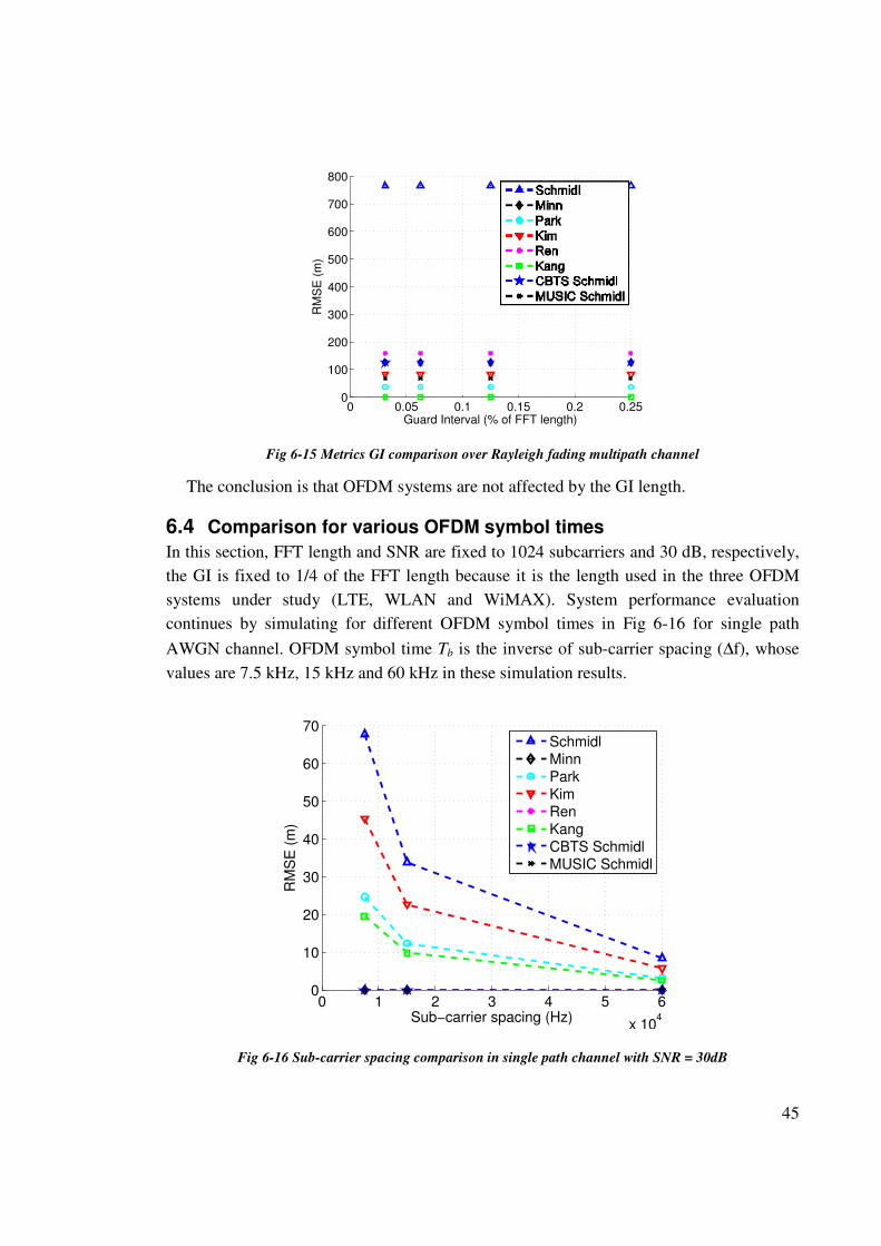
Fig 6-15 Metrics GI comparison over Rayleigh fading multipath channel

The conclusion is that OFDM systems are not affected by the GI length.

6.4 Comparison for various OFDM symbol times

In this section, FFT length and SNR are fixed to 1024 subcarriers and 30 dB, respectively,

the GI is fixed to 1/4 of the FFT length because it is the length used in the three OFDM

systems under study (LTE, WLAN and WiMAX). System performance evaluation

continues by simulating for different OFDM symbol times in Fig 6-16 for single path

AWGN channel. OFDM symbol time Tb is the inverse of sub-carrier spacing (∆f), whose

values are 7.5 kHz, 15 kHz and 60 kHz in these simulation results.

Fig 6-16 Sub-carrier spacing comparison in single path channel with SNR = 30dB

0 0.05 0.1 0.15 0.2 0.250

100

200

300

400

500

600

700

800

Guard Interval (% of FFT length)

RM

SE

(m

)

SchmidlMinn

Park

KimRen

Kang

CBTS SchmidlMUSIC Schmidl

0 1 2 3 4 5 6

x 104

0

10

20

30

40

50

60

70

Sub−carrier spacing (Hz)

RM

SE

(m

)

SchmidlMinn

Park

KimRen

Kang

CBTS SchmidlMUSIC Schmidl

46

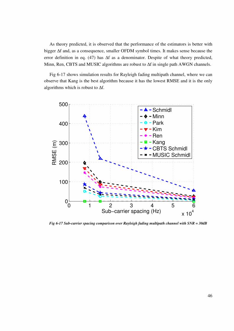
As theory predicted, it is observed that the performance of the estimators is better with

bigger ∆f and, as a consequence, smaller OFDM symbol times. It makes sense because the

error definition in eq. (47) has ∆f as a denominator. Despite of what theory predicted,

Minn, Ren, CBTS and MUSIC algorithms are robust to ∆f in single path AWGN channels.

Fig 6-17 shows simulation results for Rayleigh fading multipath channel, where we can

observe that Kang is the best algorithm because it has the lowest RMSE and it is the only

algorithms which is robust to ∆f.

Fig 6-17 Sub-carrier spacing comparison over Rayleigh fading multipath channel with SNR = 30dB

0 1 2 3 4 5 6

x 104

0

100

200

300

400

500

Sub−carrier spacing (Hz)

RM

SE

(m

)

SchmidlMinn

Park

KimRen

Kang

CBTS SchmidlMUSIC Schmidl

47

7 Conclusions and open issues

This thesis addressed the issue of preamble-based timing synchronization in OFDM

systems with the goal of cellular-based positioning. The main observation has been that

typically, the preamble-based approaches do not offer sufficient timing accuracy for

positioning applications in realistic channel conditions with low to moderate SNRs and

multipath fading.

The starting point has been the Schmidl algorithm based on a simple 2-part preamble,

which has also been the basis of all the preamble-based algorithms developed further on.

While Schmidl algorithm can be used as benchmark, it typically has the worst performance

among the considered algorithms due to a flat region in its maximum levels that is equal to

the guard interval length. Simulation results show that the lengths of the GI or the number

of used subcarriers are not affecting the system performance neither in single path nor

multipath channels (those simulations were done at equal bandwidths). It is observed that

the performance of the estimators, both in single and multipath channels, is better with

larger frequency spacing ∆f and, as a consequence, smaller OFDM symbol times. That

happens as expected, because larger frequency spacing means larger bandwidths and thus

better timing accuracy. For the same reason, it is also observed that high FFT length values

improve the system performance.

Focusing on single path channel, simulations results show that Minn, Ren, CBTS and

MUSIC algorithms are robust to OFDM symbol time. Results also show that Schmidl

algorithm is the worst one whereas Minn or Ren algorithms only work properly for SNR

values higher than 0 dB. It is observed that MUSIC is the best algorithm under study in the

full range of SNR values, and at sufficiently high FFT length, reaching zero delay error

even at -20 dB SNR, followed by Kim, Park and Kang algorithms, which have a similar

performance. It is also observed that CBTS, MUSIC and Ren algorithms are suitable for

LTE, WLAN and WiMAX because of its robustness to the number of FFT subcarriers

(MUSIC algorithm is only robust to FFT length for the algorithms based on preambles

with two identical parts). As a result, MUSIC algorithm with a preamble structure divided

into two equal parts is the best algorithm over single path AWGN channel.

Evaluating the simulator performance over Rayleigh fading multipath channel, we can

observe that Schmidl, Minn and Ren algorithms are clearly the worst among the algorithms

under study, whereas MUSIC, Park, Kim and Kang algorithms have the best (and similar)

performance. Kang algorithm is the only one that reaches zero error at the highest SNR

value, while the others may still have a residual bias or may need even higher SNR than

48

those typical to an OFDM system in moderate to good channel conditions. Furthermore,

results show that Kang is robust to the number of FFT subcarriers so it can be used in LTE,

WLAN and WiMAX. In addition to this, Kang algorithm is the only algorithm that is

robust to OFDM symbol time. Although MUSIC, Park, Kim and Kang algorithms have a

similar performance when compared for various SNR values, we can conclude that Kang

algorithm is the best one in multipath channel because it reaches zero meters error and it

can be used with the three OFDM systems and with any kind of preamble structure.

To sum up, MUSIC algorithm is the best choice over single path channels, as long as

the transmitted preamble is divided into two equal parts. For multipath fading channels,

Kang is offering the best performance among the studied algorithms. However, preamble-

based algorithms such as Kang’s have much lower implementation complexity than super-

resolution algorithms such as MUSIC. The complexity of various algorithms has not been

studied in this thesis and it remains an open issue worthy to address in the continuation.

Also, as a general conclusion, other timing algorithms than those based on preambles

should be studied and investigated for high-accuracy positioning with OFDM systems.

Such approaches are open issues in the literature regarding OFDM-based timing estimates.

49

References

[1] C. Mensing, S. Plass, and A. Dammann, “Synchronization Algorithms for

Positioning with OFDM Communications Signals,” in 4th Workshop on Positioning,

Navigation and Communication, 2007, vol. 2007, pp. 205-210.

[2] L. Dai, Z. Wang, J. Wang, and Z. Yang, “Positioning with OFDM signals for the

next- generation GNSS,” IEEE Transactions on Consumer Electronics, vol. 56, no.

2, pp. 374-379, May 2010.

[3] I. Mateu, M. Paonni, J.-L. Issler, and G. H. Hein, “A search for spectrum,”

InsideGNSS, pp. 65-71, 2010.

[4] D. Serant, O. Julien, L. Ries, P. Thevenon, M. Dervin, and G. W. Hein, “The digital

TV case,” InsideGNSS, pp. 54-62, 2011.

[5] G. Seco-granados, F. Zanier, M. Crisci, S. En-, and T. Nether-, “Preliminary

Analysis of the Positioning Capabilities of the Positioning Reference Signal of

3GPP LTE,” in 5th European Workshop on GNSS Signals and Signal Processing,

2011.

[6] C. Yang, “Signals of Opportunity for Positioning,” in ION Southern California

Section Meeting, 2011, no. 650, pp. 1-35.

[7] X. Wang, “OFDM and Its Application to 4G,” in 14th Annual Wireless and Optical

Communications Conference, 2005, p. 69.

[8] A. J. Weiss and O. Bar-shalom, “Efficient direct position determination of

orthogonal frequency division multiplexing signals,” IET Radar, Sonar and

Navigation, vol. 3, no. 2, pp. 101-111, 2009.

[9] H. Ni, G. Ren, and Y. Chang, “A TDOA location scheme in OFDM based

WMANs,” IEEE Transactions on Consumer Electronics, vol. 54, no. 3, pp. 1017-

1021, Aug. 2008.

[10] T. M. Schmidl and D. C. Cox, “Robust frequency and timing synchronization for

OFDM,” IEEE Transactions on Communications, vol. 45, no. 12, pp. 1613-1621,

1997.

[11] H. Minn, M. Zeng, and V. K. Bhargava, “On timing offset estimation for OFDM

systems,” IEEE Communications Letters, vol. 4, no. 7, pp. 242-244, Jul. 2000.

50

[12] B. Park, H. Cheon, and C. Kang, “A simple preamble for OFDM timing offset

estimation,” IEEE 56th Vehicular Technology Conference, vol. 2, pp. 729-732,

2002.

[13] J. J. Kim, J. H. Noh, and K. H. Chang, “Robust timing & frequency synchronization

techniques for OFDM-FDMA systems,” IEEE Workshop on Signal Processing

Systems Design and Implementation, vol. 2, no. 3, pp. 716–719, 2005.

[14] G. Ren, Y. Chang, and H. Zhang, “Synchronization method based on a new constant

envelop preamble for OFDM systems,” IEEE Transactions on Broadcasting, vol.

51, no. 1, pp. 139–143, 2005.

[15] Y. Kang, S. Kim, D. Ahn, and H. Lee, “Timing estimation for OFDM systems by

using a correlation sequence of preamble,” IEEE Transactions on Consumer

Electronics, vol. 54, no. 4, pp. 1600-1608, Nov. 2008.

[16] D. Serant et al., “Development and validation of an OFDM/DVB-T sensor for

positioning,” in IEEE/ION Position, Location and Navigation Symposium, 2010, pp.

988-1001.

[17] B. P. Tiwari, “LTE spectrum and Deployment Choices for Operators,” beyond4g,

pp. 1-5, 2009.

[18] IEEE 802.16 Working Group on Broadband Wireless Access, “Part 16: Air

Interface for Fixed and Mobile Broadband Wireless Access Systems,” in IEEE

Standard for Local and metropolitan area networks, 2009.

[19] D. Astély, E. Dahlman, A. Furuskär, Y. Jading, M. Lindström, and S. Parkvall,

“LTE : The Evolution of Mobile Broadband,” IEEE Communications Magazine, no.

April, pp. 44-51, 2009.

[20] IEEE 802.11 Working Group, “Part 11: Wireless LAN Medium Access Control

(MAC) and Physical Layer (PHY) Specifications,” in IEEE Standard for Local and

metropolitan area networks, 2007.

[21] S. Patil and R. Upadhyay, “A Symbol Timing Synchronization Algorithm for

WiMAX OFDM,” in International Conference on Computational Intelligence and

Communication Systems, 2011, pp. 78-82.

[22] ETSI, “LTE; Evolved Universal Terrestrial Radio Access (E-UTRA); Physical

channels and modulation,” in 3GPP TS 36.211 version 9.0.0 Release 9, 2010.

[23] L. Reggiani, “LTE systems : overview,” 2009.

[24] T. V. Waterschoot and V. L. Nir, “Analytical expressions for the power spectral

density of CP-OFDM and ZP-OFDM signals.” pp. 1-10, 2010.

51

[25] C. Liu and F. Li, “Spectrum modelling of OFDM signals for WLAN,” Electronics

Letters, vol. 40, no. 22, pp. 4-5, 2004.

[26] IEEE 802.11 Working Group, “Part 11: Wireless LAN Medium Access Control

(MAC) and Physical Layer (PHY) Specifications,” in IEEE Standard for Local and

metropolitan area networks, 2009.

[27] O.-P. Rantala, “Construction of 800 MHz mobile networks to speed up,” Press

release, 2011. .

[28] J. Zyren, “Overview of the 3GPP Long Term Evolution Physical Layer,” pp. 2-22,

2007.

[29] F. Gustafsson and F. Gunnarsson, “Mobile Positioning Using Wireless Networks,”

IEEE Signal Processing Magazine, no. 2005, pp. 41-53, 2005.

[30] K. Pahlavan and A. H. Levesque, Wireless information networks. Wiley, 1995.

[31] M. Lott and I. Forkel, “A Multi-Wall-and-Floor Model for Indoor Radio

Propagation,” in Vehicular Technology Spring Conference, 2001.

[32] J. Gu, S. Bae, and M. Chung, “Mobility-based handover decision mechanism to

relieve ping-pong effect in cellular networks,” in 16th Asia-Pacific Conference on

Communications (APCC), 2010, pp. 487-491.

[33] M. Hata, “Empirical Formula for Propagation Loss in Land Mobile Radio Services,”

IEEE Transactions on vehicular technology, vol. 29, no. 3, pp. 317-325, 1980.

[34] K. Kaemarungsi and P. Krishnamurthy, “Properties of indoor received signal

strength for WLAN location fingerprinting,” in First Annual International

Conference on Mobile and Ubiquitous Systems, 2004.

[35] A. A. Ali and A. S. Omar, “Time of Arrival Estimation for WLAN Indoor

Positioning Systems using Matrix Pencil Super Resolution Algorithm,” in 2nd

Workshop on Positioning, Navigation and Communication & 1st Ultra-Wideband

Expert Talk, 2005, pp. 11-20.

[36] F. Gustafsson and F. Gunnarsson, “Positioning using Time-Difference of Arrival

Measurements,” in IEEE International Conference on Acoustics, Speech, and Signal

Processing, 2003, pp. 8-11.

[37] P. Rong, “Angle of arrival localization for wireless sensor networks,” 3rd Annual

IEEE Communications Society on Sensor and Ad Hoc Communications and

Networks, pp. 374 - 382, 2006.

52

[38] H. Yuan, X. Hu, and Y. Ling, “New symbol synchronization algorithms for OFDM

systems based on IEEE 802.11 a,” in 6th IEEE International Conference on

Industrial Informatics, 2008, pp. 186-191.

[39] H. Minn, V. K. Bhargava, and K. B. Letaief, “A robust timing and frequency

synchronization for OFDM systems,” IEEE Transactions on Wireless

Communications, vol. 2, no. 4, pp. 822-839, May 2003.

[40] X. Li and K. Pahlavan, “Super-resolution TOA estimation with diversity for indoor

geolocation,” IEEE Transactions on Wireless Communications, vol. 3, no. 1, pp.

224–234, 2004.

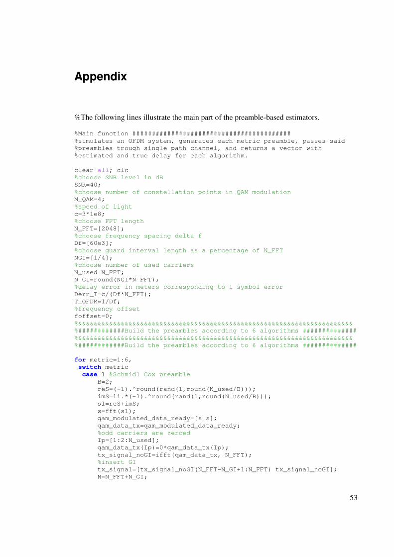
53

Appendix

%The following lines illustrate the main part of the preamble-based estimators.

%Main function #########################################

%simulates an OFDM system, generates each metric preamble, passes said

%preambles trough single path channel, and returns a vector with

%estimated and true delay for each algorithm.

clear all; clc

%choose SNR level in dB

SNR=40;

%choose number of constellation points in QAM modulation

M_QAM=4;

%speed of light

c=3*1e8;

%choose FFT length

N_FFT=[2048];

%choose frequency spacing delta f

Df=[60e3];

%choose guard interval length as a percentage of N_FFT

NGI=[1/4];

%choose number of used carriers

N_used=N_FFT;

N_GI=round(NGI*N_FFT);

%delay error in meters corresponding to 1 symbol error

Derr_T=c/(Df*N_FFT);

T_OFDM=1/Df;

%frequency offset

foffset=0;

%&&&&&&&&&&&&&&&&&&&&&&&&&&&&&&&&&&&&&&&&&&&&&&&&&&&&&&&&&&&&&&&&&&&&&&&

%############Build the preambles according to 6 algorithms ##############

%&&&&&&&&&&&&&&&&&&&&&&&&&&&&&&&&&&&&&&&&&&&&&&&&&&&&&&&&&&&&&&&&&&&&&&&

%############Build the preambles according to 6 algorithms ##############

for metric=1:6,

switch metric

case 1 %Schmidl Cox preamble

B=2;

reS=(-1).^round(rand(1,round(N_used/B)));

imS=1i.*(-1).^round(rand(1,round(N_used/B)));

s1=reS+imS;

s=fft(s1);

qam_modulated_data_ready=[s s];

qam_data_tx=qam_modulated_data_ready;

%odd carriers are zeroed

Ip=[1:2:N_used];

qam_data_tx(Ip)=0*qam_data_tx(Ip);

tx_signal_noGI=ifft(qam_data_tx, N_FFT);

%insert GI

tx_signal=[tx_signal_noGI(N_FFT-N_GI+1:N_FFT) tx_signal_noGI];

N=N_FFT+N_GI;

54

case 2 % preamble Minn

B=4;

reS=(-1).^round(rand(1,round(N_used/B)));

imS=1i.*(-1).^round(rand(1,round(N_used/B)));

s= reS+imS;

tx_signal = [-s s -s -s];

case 3 %Park

B=4;

reS=(-1).^round(rand(1,round(N_used/B)));

imS=1i.*(-1).^round(rand(1,round(N_used/B)));

s1=reS+imS;

s2=fliplr(s1);

tx_signal=[s1 s2 conj(s1) conj(s2)];

case 4 %Kim

B=4;

reS=(-1).^round(rand(1,round(N_used/B)));

imS=1i.*(-1).^round(rand(1,round(N_used/B)));

s1=reS+imS;

s2=fliplr(s1);

tx_signal=[s1 conj(s2) s1 conj(s2)];

case 5 %Ren

B=2;

reS=(-1).^round(rand(1,round(N_used)));

imS=1i.*(-1).^round(rand(1,round(N_used)));

s1=reS+imS;

%s2 CAZAC sequence of length=N/2 (Zadoff-Chu)

u=25; %root

for n=1:N_used/B

s2(n)=exp(-1i*pi*u*n*(n+1)/(N_used/B));

end

tx_signal=[s2 s2].*reS;

case 6 %Kang

reS=(-1).^round(rand(1,round(N_used)));

imS=1i.*(-1).^round(rand(1,round(N_used)));

tx_signal=reS+imS;

shift=shift_decision(s1, N_FFT);

CSP=conj(s1).*circshift(s1,shift);

p=sign(real(CSP));

q=sign(imag(CSP));

end;

%&&&&&&&&&&&&&&&&&&&&&&&&&&&&&&&&&&&&&&&&&&&&&&&&&&&&&&&&&&&&&

% +++ ++++++++++++++++++++++Channel part++++++++++++++++++++ %

%&&&&&&&&&&&&&&&&&&&&&&&&&&&&&&&&&&&&&&&&&&&&&&&&&&&&&&&&&&&&&

[ recvd_signal, D ] = Channel_part(tx_signal,SNR,foffset,T_OFDM);

%&&&&&&&&&&&&&&&&&&&&&&&&&&&&&&&&&&&&&&&&&&&&&&&&&&&&&&&&&&&&&

% ++++++++++++++++++++Delay estimators +++++++++++++++++++++ %

%&&&&&&&&&&&&&&&&&&&&&&&&&&&&&&&&&&&&&&&&&&&&&&&&&&&&&&&&&&&&&

switch metric

case 1 %Schmidl-Cox

Len_all=N_FFT; %N_FFT or length(recvd_signal);

recvd_signal_zeropad=[zeros(1,Len_all)...

recvd_signal zeros(1,Len_all)];

for d=1:2*Len_all+1,

E_Schmidl(d)=sum(abs(recvd_signal_zeropad(d+Len_all/2:d+Len_all-1)).^2);

55

P_Schmidl(d)=sum(conj(recvd_signal_zeropad(d:d+Len_all/2-

1)).*recvd_signal_zeropad(d+Len_all/2:d+Len_all-1));

end;

Schmidl_metric=(abs(P_Schmidl).^2./E_Schmidl);

%timing estimation is

derivative=diff(Schmidl_metric);

derivative=derivative/max(derivative); %normalize to 1

[~,maxipos1]=max(derivative);

[~,minipos1]=min(derivative);

%find the flat region in between max and min

I1=[min([maxipos1 minipos1]): max([maxipos1 minipos1]) ];

epsi=0.001;

I=find(abs(derivative(I1))<epsi);

while isempty(I),

epsi=10*epsi;

I=find(abs(derivative(I1))<epsi);

end;

xax=[-Len_all:Len_all];

t_est_Schmidl=xax(I1(I(1)));

case 2 %Minn

Len_all=N_FFT;%N_FFT or length(recvd_signal);

recvd_signal_zeropad=[zeros(1,Len_all) recvd_signal

zeros(1,Len_all)];

E_Minn=zeros(1,2*Len_all+1);

P_Minn=zeros(1,2*Len_all+1);

for d=1:2*Len_all+1,

for b=0:B-1,

switch b

case {0,1}

g(b+1)=(-1);

case {2,3},

g(b+1)=(+1);

end;

rx_sgn_b=recvd_signal_zeropad(d+b*Len_all/B:d+b*Len_all/B+Len_all/B-1);

E_Minn(d)=E_Minn(d)+sum(abs(rx_sgn_b).^2);

if b < B-1,

rx_sgn_bp1=recvd_signal_zeropad(d+(b+1)*Len_all/B:d+(b+1)*Len_all/B+Len_a

ll/B-1);

P_Minn(d)=P_Minn(d)+g(b+1)*(sum(conj(rx_sgn_b).*rx_sgn_bp1));

end;

end;

end;

Minn_metric=(B/(B-1)*abs(P_Minn)./E_Minn).^2;

%timing estimation is

[~, maxipos1]=max(Minn_metric);

t_est_Minn=maxipos1-Len_all-1;

case 3 %Park

Len_all=N_FFT; %N_FFT or length(recvd_signal);

recvd_signal_zeropad=[zeros(1,Len_all) recvd_signal

zeros(1,Len_all) zeros(1,Len_all)];

for d=1:2*Len_all+1,

P_Park(d)=sum((recvd_signal_zeropad(d:d+Len_all/2)).*fliplr(recvd_signal_

zeropad(d+Len_all/2:d+Len_all)));

56

E_Park(d)=sum(abs(recvd_signal_zeropad(d:d+Len_all/2)).^2);

end;

Park_metric=(abs(P_Park)./(E_Park)).^2;

%timing estimation is

[~, maxipos1]=max(Park_metric);

t_est_Park=maxipos1-Len_all/2;

case 4 %Kim

Len_all=N_FFT; %N_FFT or length(recvd_signal);

recvd_signal_zeropad=[zeros(1,2*Len_all) recvd_signal

zeros(1,2*Len_all)];

for d=1:2*Len_all+1,

E_Kim(d)=sum(abs(recvd_signal_zeropad(d+Len_all/2:d+Len_all-1)).^2);

P_Kim(d)=sum(recvd_signal_zeropad(d+Len_all/2:d+Len_all).*fliplr(...

conj(recvd_signal_zeropad(d+Len_all:d+Len_all+Len_all/2))));

end;

Kim_metric=(abs(P_Kim)./E_Kim).^2;

%timing estimation is

maxipos1=find(Kim_metric>1);

t_est_Kim=maxipos1(end)-Len_all-2;

case 5 %Ren

Len_all=N_FFT;

recvd_signal_zeropad=[zeros(1,Len_all) recvd_signal

zeros(1,Len_all) zeros(1,Len_all)];

for d=1:2*Len_all+1,

P_Ren(d)=sum(s1(1:Len_all/2).*s1(1+Len_all/2:Len_all).*conj(...

recvd_signal_zeropad(d+1:d+Len_all/2)).*recvd_signal_zeropad(d+1+Len_all/

2:d+Len_all));

E_Ren(d)=0.5*sum(abs(recvd_signal_zeropad(d:d+Len_all-

1)).^2);

end;

Ren_metric=(abs(P_Ren)./E_Ren).^2;

%timing estimation is

[~, maxipos1]=max(Ren_metric);

t_est_Ren=maxipos1-Len_all;

case 6 %Kang

Len_all=N_FFT; %N_FFT or length(recvd_signal);

recvd_signal_zeropad=[zeros(1,Len_all) recvd_signal

zeros(1,Len_all)];

for d=1:2*Len_all+1,

V=conj(recvd_signal_zeropad(d:d+Len_all-

1)).*circshift(recvd_signal_zeropad(d:d+Len_all-1),shift);

E_Kang(d)=norm(real(V))+norm(imag(V));

P_Kang(d)=real(V)*p'+imag(V)*q';

end;

Kang_metric=(P_Kang./E_Kang).^2;

%timing estimation is

[maximum, ~]=max(Kang_metric);

maxipos1=find(Kang_metric>maximum-1);

t_est_Kang=maxipos1(end)-Len_all-1;

end;

end;

57

disp(['True Delay and Estimated delays in meters for Schmidl, Minn, Park,

Kim, Ren and Kang'])

[D t_est_Schmidl t_est_Minn t_est_Park t_est_Kim t_est_Ren

t_est_Kang]*Derr_T

%Following function is used to simulate the system channel

%Channel_part function #########################################

function [ recvd_signal,D ]=Channel_part(tx_signal,SNR,foffset,T_OFDM);

%Add random delay; here given in samples D=round(10*rand(1,1)); del_sig=[zeros(1,D) tx_signal(1:end-D)]; %Add AWGN s=randn(1,length(del_sig)); sigma=sqrt(1/(10^(SNR/10))); %normalize sigma to signal power: power_timedomain = mean(abs(x).^2)) sigma=sigma*sqrt(mean(abs(tx_signal).^2)); S=(s-mean(s))/sqrt(var(s)); noise=sigma.*S; awgn_signal=del_sig.*exp(1i*2*pi*foffset*[1:length(del_sig)]/N)+noise; %Pass the ofdm signal through the channel recvd_signal=awgn_signal;

end

%Following function is used to find shift value for Kang algorithm

%shift_decision function #########################################

function [ out ] = shift_decision( signal, Nfft ) for i=1:length(signal) C = conj(signal).*circshift(signal,i); autocor = xcorr(C); max_corr = max(autocor); m = (mean(autocor(1:Nfft-1)) + mean(autocor(Nfft+1:end)))/2; shift_out(i)=(max_corr-m); end

[~, out] = max(shift_out); end