Lee1

Lab2:DigitalSignalProcessingandVibrations

AustinLeeM006_1

DueDate:11/21/16

Lee2

TableofContentsABSTRACT............................................................................................3INTRO....................................................................................................4PROCEDURE.....................................................................................14

DigitalSignalProcessing.....................................................................14Vibrations...................................................................................................19

RESULTS............................................................................................26RESULTSFORDSPLAB................................................................................26RESULTSINVIBRATIONSLAB.....................................................................43

CONCLUSION....................................................................................52REFERENCES....................................................................................52APPENDIX.........................................................................................53DIGITALSIGNALPROCESSING.....................................................................53VIBRATIONS................................................................................................151

EXTRACREDIT:LAB2CDRONEDROPTESTS.....................207ABSTRACT:..................................................................................................207INTRO...........................................................................................................207PROCEDURE................................................................................................208RESULTS......................................................................................................210CONCLUSION...............................................................................................214REFERENCES...............................................................................................214APPENDIX....................................................................................................215

Lee3

AbstractInthisreportwesimulatedandexperimentedwithdigitalsignalprocessing

andvibrations.Inonepartwegeneratedalreadyknownsignalsandintheotherwestimulatedabeamwithtwodifferenttypesofwaysandrecordedtheresponseofthesystem.

First,weusedLABVIEWtocreatesinusoidal,square,andsawtoothwaves.Wegeneratedthemmultipletimeswithvaryingfrequencies,resolution,samplefrequencies,numberofsamples,filters,andamplitudes.Thisgaveusanunderstandingofhowthewaveformchangedbasedonthesemanyfactors.

Wethentookthedataandplotteditbothinthetimedomain,Voltagevs.

Time,andinthefrequencydomain,Voltagevs.Frequency.Nowweappliedourbasicunderstandingtotrytofurtherlearnaboutaliasing,clipping,andquantization,andhowtheyaresourcesoferrorwheneverdigitizingsignals.

Incertaininstances,wedidnotencounteranyerrorbecauseweintentionallymadeitsothesignalwouldnotbeclippedoraliased.AfterreviewingtheplotsandmakingNyquistfoldingdiagramswesawsignalsaliasedduetoinsufficientsamplefrequencies,theoutcomeofthesignalifithadbeenclipped,andthequantizationerrorwhentheresolutionwastolow.Wecancontrolallthefactorsoferrortosomeextentexceptforquantizationerror;itisunavoidablewheneverconvertinganyanalogsignaltoadigitalsignal.

Wewillalsodealwithresultsthatdonotreflectourpreconceivednotionof

theresults.Theresultsarefarofffromwhatweexpectedandsinceweourgeneratingthewaveforms,thereforetherecouldn’tbeanypossibleerrorinthemanufacturingofthewave,weencounteredoursignalbeingaliasedorclipped.Bothoftheseerrorsresultedin“false”dataresultswheretheamplitude,inthetimedomain,orthefrequencywasnotwhatshouldhavebeen.

WeusedFourieranalysistofindFouriercoefficientsineachspecificcaseand

usedthemtoreconstructtheoriginalwaveformusingasumofsinusoidalwaves.AllofthesefunctionswereoddfunctionswhichmeanstheFouriercoefficients𝑎! = 0and𝑎! = 0.AnalyzingthedatainMATLABwesawresultsthatmatchedthetheory.

Nowthatweknowwhattolookforwhenanalyzingsignals,wethenlookedattheresponseofametalbeamattachedtoanaccelerometerandtheresponseofanimpact.Wesimulatedandexperimentallytestedthisresponsewithawiderangeofchangingfactorslikethebeammaterial,endmass,andthebeam’slength.

TheuseofdigitalsignalprocessingiscrucialsinceeverythingaroundusisanalogandtoanalyzeortransfertheinformationthesignalneedstobeconditionedandputthroughanA/Dconverter.

Lee4

Intro Inthislabwedealwithsignals,signalsaredefinedasanytimevaryingmeasurement.Signalscaneitherbeanalog,signalthatcanachieveaninfinitesetofvalueswithinaspecificrange,ordigital,signalthatcanbeafinitesetofvaluesoveragivenrange.Wespecificallyareinterestedindigitalsignalprocessing,whichisthenumericmanipulationofsignals,usuallywiththeintenttomeasure,filter,produce,orcompresscontinuousanalogsignals.Digitalsignalprocessing(DSP)isaroundusmorethanwethink,telecommunications,audio,sonar,digitalphotography,radarandmanymoretechnologiestoexist.Intheflowchartbelow,

wecanseethattogetfromananalogsignaltoadigitalsignalonacomputerordevice,onemustconditionthesignalbymeansoffilters,amplifiersoretc.ThenpasstoanA/Dconverter.Duringthisprocessmultipleerrorscanoccur.Theyareclipping,formofdistortionthatlimitsasignalonceitexceedsacertainthreshold,quantizationerror(Q),errorwhenitisconvertedfromanalogtodigital,

𝑄 =𝐵𝑖𝑝𝑜𝑙𝑎𝑟 𝑅𝑎𝑛𝑔𝑒

2!!! 𝑁 = 𝑟𝑒𝑠𝑜𝑙𝑢𝑡𝑖𝑜𝑛oraliasing,themisidentificationofthesignalfrequencyintroducingdistortionerrors.TocombataliasingwecanuseNyquist’stheoremwhichstatesthatthesignalmustbesampledatleasttwicethemaxfrequencyotherwisethehighfrequencysignalwillbemisrepresented. Topreventaliasingfromhappening,onethingwecandotothesignalistouseafilter.Itisadeviceorprocessthatremovessomeunwantedcomponentsofasignal.Forexample,alowpassfilteronlyallowsfrequencieslowerthanthecutoffvaluetopass.CombiningalowpassfilterwiththeNyquistfrequencyweget,

AnalogTransducer

SignalConditioning

Analog/DigitalConverter Computer

LowPassFilter Amplifier

Amplitude(V)

Frequency(Hz)

Cutofff=1/2T

(fig.1)

(eq.1)

(fig.2)

Lee5

ahighpassfilterdoestheoppositeandonlyallowsfrequencieshigherthanthecutoffvaluetopass

Abandpassfiltertakesahighpassandlowpassfilterandcombinestheminseriesgiving,

Anothertypeoffilteristhebandrejectfilter,whichcombinesalowpassfilterandhighpassfilterinparallel.

Amplitude(V)

Frequency(Hz)

Cutoff

Amplitude(V)

Frequency(Hz)Cutoff

Cutoff

LowPass HighPass

LowPass

HighPass

Amplitude(V)

Frequency(Hz)

Cutoff

Cutoff

(fig.3)

(fig.4)

(fig.5)

Lee6

FourierSeriesCoefficientswerederivedfromtheequationsbelow(thefullderivationscanbefoundintheappendix),withtheonlynonzerotermbeing𝐵!sincetheyareoddfunctions,Tbeingperiod,tistime,𝑓!beingtherepetitionrate.FindingtheFouriercoefficientsallowsustoFouriertransformfromthetimeseriesintothefrequencyseries.Ifyouhaveacontinuoustimeseriesthenyoualsohaveacontinuousfrequencyseries.Thisiswhatallowsustogofromthetimeintofrequency.SinWaveFourierCoefficients

𝑎! =1𝑇 5sin (2𝜋𝑓!𝑡)

!

!𝑑𝑡

𝑎! = 0

𝑎! =2𝑇 5sin (2𝜋𝑓!𝑡)cos (2𝜋𝑓!𝑡𝑛)

!

!𝑑𝑡

𝑎! = 0

𝑏! = 2𝑇 5 sin 2𝜋𝑓!𝑡 sin 2𝜋𝑓!𝑡𝑛

!

!𝑑𝑡

𝐵! = 5

SquareWaveFourierCoefficients

𝑎! =1𝑇 5 𝑑𝑡 +

1𝑇 −5 𝑑𝑡

!

!!/!

!/!

!

𝑎! = 0

𝑎! =2𝑇 5 cos 2𝜋𝑓!𝑡𝑛

!!

!𝑑𝑡 +

2𝑇 −5 cos 2𝜋𝑓!𝑡𝑛

!

!!

𝑑𝑡

𝑎! = 0 ,𝑛 = 1,2,3,… ,21

𝐵! =2𝑇 5𝑠𝑖𝑛 2𝜋𝑓!𝑡𝑛 𝑑𝑡 +

2𝑇 −5𝑠𝑖𝑛 2𝜋𝑓!𝑡𝑛 𝑑𝑡

!

!!/!

!/!

!

(eq.2)

(eq.3)

(eq.4)

(eq.5)

(eq.6)

(eq.7)

Lee7

𝐵! = −10 cos 𝜋𝑛

𝜋𝑛 +5cos (2𝜋𝑛)

𝜋𝑛 n=1,3,5,7….SawtoothWaveFourierCoefficients(A=amplitude)

𝑎! =1𝑇

2𝐴𝑡𝑇 𝑑𝑡

!/!

!!/!

𝑎! = 0

𝑎! = 2𝑇

2𝐴𝑡𝑇 cos (2𝜋𝑓!𝑡𝑛)

!/!

!!/!𝑑𝑡

𝑎! = 0

𝑏! = 2𝑇

2𝐴𝑡𝑇 sin (2𝜋𝑓!𝑡𝑛)

!/!

!!/!𝑑𝑡

𝑏! = −2𝐴 cos 𝜋𝑛

𝜋𝑛

Fourier Series:

𝑦(𝑡) = 𝐴0 + ∑∞𝑛=1(𝐴𝑛 cos 𝑛𝑡 + 𝐵𝑛 sin 𝑛𝑡)

TohelpvisualizealiasingweconstructedNyquistplots,whichshowthe

Nyquistfrequencyandwhattheoriginalfrequencywasbeforeitwasaliased.AnexampleofthiswouldbetheKrohn-HiteFilter3.2Krohn-HiteFilterNyquistPlot

500Hz

1000Hz1500Hz

2000Hz 2500Hz

0Hz300Hz

700Hz

(eq.8)

(eq.9)

(eq.10)

(fig.6)

(eq.11)

Lee8

Wecanseethatthefrequencyshouldbe700Hzbutonthefrequencyvs.Amplitudegraphitwillonlyhaveasingleamplitudeat300Hz. Certainapplicationsrequiredifferentsignalprocessestocorrectlymanipulatetheanalogsignaltofittherequirements.Buttheprocessofhowthesignalstartsfromanalogandendsupdigitalarethesame.Whetheritisthehardwarethatcapturespeoplesvoicesandconvertsittotextonaphoneorfly-by-wireflightcontrolsinplaneswhereitconvertsthepilot’smanualinputintoadigitalinputwhichcontrolstheplane. Now,havingabettersenseofhowasignalmaybedistortedorskewbaseonthesignalconditioningandmultipleformsoferrorthatcouldoccurwecanconfidentlyanalyzethevibrationssystemintheshakerandhammertest. Inthevibrationssectionofthislabweexperimentedwithabeamsresponsewhenoscillating,repetitivemotionofanobjectaroundanequilibriumpoint,andtheresponseofthebeamwhenimpacted.Wecanmodelthissystemasaspringdampedmasssystem(harmonicoscillation).Thenwecanusthesecondorderdifferentialequationofaspring-massdampedsystemtofindnaturalfrequency.k=springconstant(N/m)m=mass(kg)R=DampingCoefficient(c)(N*s/m)

(fig.7)

Lee9

x=position(m)v=velocityor𝑥(m/s)F=force(N)

𝐹! = 𝑚𝑎

𝐹 𝑡 − 𝑘𝑥 − 𝑐𝑣 = 𝑚𝑎

𝐹 𝑡 = 𝑚𝑎 + 𝑐𝑣 + 𝑘𝑥

𝑚𝑥 + 𝑐𝑥 + 𝑘𝑥 = 𝑓(𝑡)or

𝑥 +𝑐𝑥𝑚 +

𝑘𝑥𝑚 =

𝑓(𝑡)𝑚

Takingthisspring-massdampedsystemwethenapplyittoourcaseofabeamandfind

F(t)

kx

cv

L

F

t

w

δ

(fig.8)

(eq.12)

(fig.9)

x

y

Lee10

Fromthiswecansummomentsandfindthespringconstantandthemassequivalence.

𝛿 = !!!

!!" 𝐼 = !

!"𝑤𝑡!

𝑘 =𝑃𝛿 =

3𝐸𝐼𝐿!

Examiningtheequationofspringconstant,wecanseeitisproportionaltoYoung’sModulusandIthesecondmomentofinertia.Bychangingthelengthintheexperimentalsectionandthetypeofmaterialinthesimulationweshouldseevaryingspringconstants.Massequivalencebasedonthederivationinclass:

𝑚!" =33140 ∗𝑚!"#$ +𝑚!"# !"##

Naturalfrequency:

𝑊! =!

!!"rad/sorHz

DampeningRatio(𝜉):

𝜉 =𝑐

2𝑚!"𝑊! 𝑐 = 𝑑𝑎𝑚𝑝𝑖𝑛𝑔 𝑐𝑜𝑒𝑓𝑓𝑖𝑐𝑒𝑛𝑡

If𝜉 > 1,overdampedIf𝜉 < 1,underdampedIf𝜉 = 1,criticallydampedIf𝜉 = 0,un-dampedNowtheequationcanbeputintotheform,

𝑥 + 2𝜉𝑊!𝑥 +𝑊!!𝑥 = 𝐴𝑓(𝑡)

(eq.13)

(eq.14)

(eq.15)

(eq.16)

(eq.17)

Lee11

Condition1:NoDampening(c=o)

𝑚𝑥 + 𝑘𝑥 = 𝑓(𝑡)Condition2:Damped

𝑚𝑥 + 𝑐𝑥 + 𝑘𝑥 = 0

𝜆!,! =!!!! !!!!!"

!!

If𝑐! − 4𝑚𝑘 > 0 , 𝜆!,!realàoverdampedIf𝑐! − 4𝑚𝑘 < 0,𝜆!,!complexàunderdampedIf𝑐! − 4𝑚𝑘 = 0 , 𝜆!,!realàcriticallydampedDampedNaturalFrequency:

𝑊! =𝑊! 1− 𝜉! 𝑟𝑎𝑑𝑠

Toconvertrad/stoHz:

𝑓 =𝑤2𝜋

Examples:un-damped(c=0),underdamped(c=100),andoverdamped(c=604&

900)

(eq.18)

(eq.19)

(eq.20)

(eq.21)

(fig.10)

Lee12

TheEulerformulaforcomplexroots:

𝐴𝑐𝑜𝑠 𝑊!𝑡 + 𝐵𝑠𝑖𝑛(𝑊!𝑡) Phaselagisthedifferencebetweentherealandimaginaryoscillatingwavesandwhentheyareequalitisinphaseandwhenthewavesarecompletelyoppositefromoneanotheritisoutofphase.UsingthetransferfunctionbuiltintoMATLABwecancalculatephaselag.ForsignalswedonotknowthemathematicalsolutiontousingFourieranalysisallowsustofindthecomplexrootstosignalandplottingthemagnitudeofresponse(Glauser).PhaseLag:

𝜙 = 𝑡𝑎𝑛!!𝐵𝐴 𝐴 = 𝑟𝑒𝑎𝑙 𝑝𝑎𝑟𝑡;𝐵 = 𝑖𝑚𝑎𝑔𝑖𝑛𝑎𝑟𝑦 𝑝𝑎𝑟𝑡

TransferFunction:Input->x(t)=𝑥(𝑓)Output->y(t)=𝑦(𝑓)TransferFunction𝐻 𝑓 =!"#$"#

!"#$%= !(!)

!(!) 𝑤ℎ𝑒𝑟𝑒 𝐻 𝑓 𝑖𝑠 𝑐𝑜𝑚𝑝𝑙𝑒𝑥

MagnitudeofResponse:

𝑥 𝑓 = 𝑟𝑒𝑎𝑙𝑥 𝑓 + 𝑖𝑚𝑎𝑔𝑥(𝑓)𝑦 𝑓 = 𝑟𝑒𝑎𝑙𝑦 𝑓 + 𝑖𝑚𝑎𝑔𝑦(𝑓)

𝐻(𝑓) = 𝑟𝑒𝑎𝑙𝐻(𝑓) ! + [𝑖𝑚𝐻 𝑓 ]! ResonanceFrequency:

𝑊! =𝑊! 1− 2𝜉! Resonancefrequencyistheresultofexternalforcevibratingatthesamefrequencyasthenaturalfrequency.Thisisfrequencyiscrucialtounderstandwhendesigningsomething.Ifyoudesignsomethingthatvibratesatitsresonancefrequencyitwillleadtodisastrousconsequencesandnotbesafeoruseable.ForexampletheTacomaNarrowsBridge(UniversityofWashington,4),strongwindsmadethebridgeresonateatitsnaturalfrequency,whichleadthebridgesurfacetodeflectatitsmaximumamplitudeandfailatsomepoint.

(eq.22)

(eq.23)

(eq.26)

(eq.25)

(eq.24)

Lee13

Giventhatwewereconvertinganalogsignalsfromthebeamtodigitalsignalssothatwecouldanalyzethedataquantitativelywehavetoaccountforuncertaintyintheinstrumentsusedtomeasuretheresponse.UncertaintywascalculatedusingZero-orderuncertaintyandRSSmethodtocalculatepropagateduncertainties:

𝑢 = !

!!!𝑅𝑒𝑠𝑜𝑙𝑢𝑡𝑖𝑜𝑛

1. 𝑉𝑜𝑙𝑡𝑎𝑔𝑒 𝑅𝑒𝑠𝑜𝑙𝑢𝑡𝑖𝑜𝑛 = !"!!"#$% !"#$%&!!!!

where N is the resolution of the ADC in bits (13 bits for the ADC’s used in the experimental section). The bi-polar range of the ADC’s we use is +/- 10V.

2. 𝑇𝑖𝑚𝑒 𝑅𝑒𝑠𝑜𝑙𝑢𝑡𝑖𝑜𝑛 = !!"#$%& !"#$%#&'(

3. 𝐹𝑟𝑒𝑞𝑢𝑒𝑛𝑐𝑦 𝑅𝑒𝑠𝑜𝑙𝑢𝑡𝑖𝑜𝑛 = !"#$%& !"#$%#&'(# !" !"#$%&'

Uncertaintyinthevibrationslabincorporatedthesameuncertaintieswecalculatedbeforeandtheninlength(m),width(m),thickness(m),dampingcoefficient(N*sec/m),density,andYoung’sModulus.

Uncertaintyinlength:

𝑈 = 12 𝑥 𝑡𝑎𝑝𝑒 𝑟𝑒𝑠𝑜𝑙𝑢𝑡𝑖𝑜𝑛 (𝑟𝑒𝑠𝑜𝑙𝑢𝑡𝑖𝑜𝑛 =

132)

Uncertaintyinwidthandthickness:𝑈 = !

! 𝑥 𝑐𝑎𝑙𝑖𝑝𝑒𝑟 𝑟𝑒𝑠𝑜𝑙𝑢𝑡𝑖𝑜𝑛 ( 𝑟𝑒𝑠𝑜𝑙𝑢𝑡𝑖𝑜𝑛 = .00001)

UncertaintyinDampingCoefficient:𝑈 = .005

UncertaintyinModuli:𝑈 = .005

UncertaintyinDensity:𝑈 = .005

Ourresultsfromboththesimulatedandexperimentalportions(appendix)werenearlyidenticalgivingaverylowuncertaintyinsomecases. Thesetypesofteststhatweconductedcanbeclassifiedasnon-destructivetestingtechniquebecauseyoucanevaluatethepropertiesofthematerialwithoutcausinganytypeofpermanentdamagetooccur. Applyingthistorealworldapplicationslikestructuralapplicationscanpreventmajorcatastrophesfromoccurring.Forinstance,ifaregionintheworldliesonafaultlineandispronetoearthquakesdesigningthebuildingtonothavethesameresonancefrequencycanmakethedifferenceinwhetherthebuildingisstandingandpeoplearesafeorifthebuildingcollapsesandpeoplelosingtherelives(WilliamHarris,7).Similartotheimpactexperimentwiththehammer,ifan

(eq.27)

(eq.28)

(eq.29)

(eq.30)

(eq.31,32,33)

Lee14

engineerisdesigningastructuretowithstandinimpact,theymustcalculatehowtheapplicationabsorbsenergy,themaximumdeltaitseesfromtheimpact,andthebestmaterialwiththerightspringconstanttosuitetheapplication.

Procedure

DigitalSignalProcessing Required Equipment:

• National Instruments system with LabVIEW • A/D Converter

o 13 bits

o 48 KS/s – max sample rate

o AI FIFO 512 bytes

o Input range +/- 10 Volts

o Working voltage +/- 10 Volts

o Input impedance 144 kΩ

• Function Generator (B&K sine and square wave generator) • 1 SMB to BNC cable

2.0 Simulation 2.1 Digital Oscilloscope Simulation In this section, you will be simulating the experiment from Section 3.1. Here an A/D converter is not used as the signals are digitally generated within the computer itself. Be sure to consider this when comparing the experimental results to the simulation results. Important Note when saving your data: Make sure you keep track of the file names in your lab notebook!

Lee15

• Select a “Sine wave” as the input function using the pull down menu from the “Input Function” tablet.

• Set the frequency control (located in the “Input Function” tablet) to resolve a 700 Hz wave.

• Make sure the amplitude display is set to 5.0 volts • In the “Acquisition Control” tablet, set the sampling frequency to 25

kHz and the number of samples to 4096. • Select “12 bit resolution” from the pull down menu. • Select “bipolar range -- +/- 10 volts” from the pull down menu. • In the “Filtering” tablet, set the low pass filter setting to "OFF" as to

dismantle the simulated filter. • Press the "Run arrow” located in the top of the LabVIEW tool bar. • Measure the frequency of the sine wave from the plot using the cursor

controls (top graph). • Use the cursor controls to get an accurate value of the frequency at

which the peak is located in Fourier space (bottom graph). • Note the signal is not aliased at this sampling frequency. Why? • Recheck all the settings, both on the function generator and the VI

panel. If everything is correct, change the “Write to File” command to “Yes” and rerun the program, as it will be saved this time.

• At this point, it is recommended that the “Write to File” command be deactivated after each section as to prevent excessive files from being generated.

2.2 Fourier Analysis Simulation In this case, you will be simulating the experiment from section 3.0 using two waveforms, a square wave and a triangle wave, in both the time and frequency domains. Be sure to make the appropriate comparisons to theory and to the experiment in your report.

• Select the square wave from the input function pull down menu. • Set the waveform frequency to 700 Hz. • Set the sampling frequency to 25 kHz. • Use the same voltage and bit-resolution settings from the previous

sections. • Activate the low pass filter with a cut-off frequency of half or less than

half of the sampling frequency. • Press the "Run" arrow. • Use the cursor controls to get the amplitude and frequency values of the

time trace from the oscilloscope display (top graph). Note the shape of the wave.

Lee16

• Repeat this section by deactivating the filter. Note the changes in the shape of the square wave. What caused this change in the square wave to occur?

• Use the cursor controls to get accurate amplitude and frequency values of the peaks from the fft spectrum analyzer (bottom graph) from the filtered case.

• Remember to "Save" the data. • Repeat this procedure for the sawtooth wave. Further investigations

with other waveforms may be performed as well. The triangle and Gaussian noise waveforms are available in this simulation.

You should compare your results with those from the experiment and theory. Are the amplitudes of the peaks in the frequency domain consistent between experiment, simulation and theory? Also, be sure to include an uncertainty analysis. How does uncertainty play a role with simulated data? What are the advantages and limitations of the three methods of analysis (experiment, simulation and theory). 2.3.1 Quantization Error and Resolution

• Select the sine wave from the input function pull down menu. • Set the waveform frequency to 700 Hz. • Set the waveform amplitude to 5.00 volts. • Set the sampling frequency to 25 kHz. • Use the same voltage and bit-resolution settings from the previous

sections. (+/-10 volts and 12 bit, respectively) • Activate the low pass filter with a cut-off frequency of half or less than

half of the sampling frequency. • Press the "Run" arrow. • Note the resolution (smooth shape) of the wave. • Repeat this section, but with the “4 bit Resolution” selected from the

pull down menu in the “Acquisition Tablet” • Note the change in the resolution of the wave. • From your understanding of quantization error, what has caused this to

occur, and should this be a concern for someone attempting to measure digital signals?

• Remember to "Save" the data. It is optional to repeat this for the other waveforms. An interesting point of discussion is the dependence / independence of the square wave to the number of bits in the data acquisition system.

2.3.2 Clipping • Continue working with the sine wave from the input function pull down

menu. • Set the waveform frequency to 700 Hz.

Lee17

• Set the waveform amplitude to 5.00 volts. • Set the sampling frequency to 25 kHz. • Use the “12 or 16 bit resolution” setting • Select the “bipolar voltage +/-10.0 volts”. • Use your understanding of filtering to determine whether the low pass

filter should or should not be activated. • Activate the “Write to File” and press the "Run" arrow. • Now, repeat the simulation with a “bipolar voltage +/-1.0 volts”. • Note the clipping of the input sine wave’s peaks. • Why is this important, and when should one consider this? • Don’t forget to write this to file.

3.0 Experiment Important Note when saving your data: Make sure you keep track of the file names in your lab notebook! In this portion of the lab, you will use a digital computer to acquire and analyze actual signals from the necessary hardware using an A/D converter. 3.1 Digital Signal Acquisition (Digital Time History and Spectra)

• Set the waveform selector to a sine wave. • The function generator frequency should already be set to 700 Hz, do

not touch the knob. • The function generator amplitude should already be set to 5.0 V, do not

touch the knob. • On the Labview VI select a sampling rate of 25 kHz and set the number

of samples to acquire to 8192. • Press the "Run arrow” located in the top of the LabVIEW tool bar. • Measure the actual frequency of the sine wave. (NOTE: The mouse

can be used to move the cursors on the plots.) • Use the cursor to get an accurate value of the frequency at which the

peak is located. Compare these values with those obtained from the simulation.

• Note that at this frequency the signal is not aliased. Why? • Recheck all the settings, both on the function generator and the VI

panel. If everything is correct, activate the “Write to File” and rerun this section.

3.2 Anti-Aliasing and filtering •€€€€Repeat the process from above for a sampling frequency of 1000

Hz. • Note that at this frequency the signal is aliased. Why?

Lee18

• Recheck all the settings, both on the function generator and the VI panel. If everything is correct, activate the “Write to File” and rerun this section.

•€€€€€€Now run the function generator through the Krohn-Hite filter • Note that at this frequency the signal is aliased. Why? • Recheck all the settings, both on the function generator and the VI

panel. If everything is correct, activate the “Write to File” and rerun this section.€€€

3.3 Fourier Analysis Experiment In this part of the experiment, you will examine a square wave, in both the time and frequency domains. You will obtain enough information here to compare your results to Fourier theory and to the simulation data. Make sure that you perform these comparisons in your report.

• Select a square waveform at 700 Hz • Select a sample rate of 25 kHz. • Make sure you obtain the amplitude and frequency of the wave from the

time trace. (NOTE: This can be done quickly in the lab, using the mouse driven cursors on the VI panel, or later by slowly scanning a spreadsheet column containing thousands of points.)

• Make sure to get a value of the frequency and amplitude of the various peaks in the frequency domain.

• Why is there more than one peak? Why are the peaks in the Fourier domain at their particular frequencies? Are the amplitude of the peaks consistent with those from theory? Be sure to include the relevant uncertainty analysis for the measured quantities

• Repeat the process for a sawtooth waveform.• Change over to the B&K function generator on the table and make sure

it’s on the white noise setting. Set the sampling frequency to its highest setting (40kHz) in the vi. Set the low-pass filter cut-off frequency accordingly to prevent aliasing. Analyze the decay of the frequency spectrum around its Nyquist frequency. A good filter has the ability to decay rapidly, where as poor filters decay much more gradually, thus allowing aliased signals to infiltrate and corrupt the digitized data. Some Questions you should address

• Why do the aliased signals from the simulation and experimental cases without the filter, show up at this particular frequency? Either use the calculations shown in the notes or the aliasing diagram to demonstrate why the aliased signal shows up at that particular frequency.

• Why does the aliased signal disappear when low pass filtered at half of the sampling frequency?

• What are some examples of aliasing in other real world situations?

Lee19

• What would the frequency spectrum look like for a white noise input function, sampled at 25kHz and band pass filtered between 5kHz and 20kHz.

Vibrations

1.2 Required Equipment:

o Shaker (single degree of freedom) o Power supply for shaker o B & K function generator o 2 accelerometers o 2 BNC to SMB coaxial cables o Carbon steel bar o Charge Amplifier (power supply for the accelerometers) o National Instruments PXI system with LabVIEW 9 (or 10) § NI cDAQ-9172 series controller with 2.39 GHz Processor, 1.0 GB of RAM, 20GB memory with Windows XP. § NI 9234 A/D card with 4 channel, +/- 5 volts, 24 bit IEPE and AC/DC Analog Input Module. § 24 bit resolution § Analog low pass filters § 50 kHz max sampling rate. o Measuring tape or ruler

1.3 Experiment Apparatus:

The apparatus consist of a steel cantilever beam mounted on a single degree of freedom shaker. Two accelerometers are mounted to the beam, one at the base (input) and one at the free end (response) of the beam. The charge amplifiers supply excitation to the transducers. In addition, the base of the beam is fixed using a removable clamp that can be used to adjust the length of the beam (which will change the natural frequency of the system).

The LabVIEW software will be used to acquire the experimental data. The format for some of the files is found following the "Topics for Discussion".

2.0 Experiment

Procedure:

Lee20

Measure the dimensions of the beam for use in calculation of the theoretical natural frequency. We will be performing this test for three different bar lengths. Be sure to include the uncertainty associated with the measuring device. Let’s concentrate on the first bar length for now. Also, note the material of the beam (most likely carbon steel). The mass of the accelerometer is small and has little effect on the system’s response. Be sure to measure only the portion of the beam that will be vibrating. Do not include the portion of the beam located in the clamp.

2.1 The Shaker Test

In this experiment, the bars forced frequency is investigated. When the forcing frequency matches the beam's natural frequency, resonance is observed.

We begin by sweeping through several input functions to see where the different modes of the system’s natural frequency exist. .

o Make sure that the bar is clamped securely for a given bar length. o Turn on the accelerometer’s charge amplifier and wait approximately 5 minutes for the accelerometers to stabilize. o Turn on the power supply to the shaker and power on the input function generator (B & K unit). o Set the output function on the function generator to sweep mode. This will increase the input frequency of the shaker table from 2Hz to 30Hz and back to 2Hz at a constant rate of 1 Hz/second with a given amplitude. o Record the resonance frequency (s) observed.

2.2 The Accelerometer Test

In this test, the natural frequency and damping of the bar’s free response is investigated.

o Ensure that the first accelerometer (at the beams free end) is connected to channel 1 of the charge amplifier’s input. Use the coaxial cable to connect the output from the power supply (channel 1) to channel 0 of the PXI system. Do the same for the second accelerometer located at the base of the cantilever beam. That is channel 2 of the charge amplifier is connected to channel 1 of the PXI system. o Open the VI (located on the desktop) "VIBEXP2013.vi" and make an observation of the various tabs and controls on the screen. The top plot is the time series response of the two accelerometers, whereas the bottom two plots are the frequency spectra of the accelerometers 1 and 2 respectively. o We will be sampling at 3 KHz, low pass filtering at approximately 1 KHz, and acquiring 8192 samples per scan. The "Save Spectra & Time series Data?" and "Save Peak Data" can be activated and/or deactivated at any time during the experiment.

Lee21

2.2.1 Recording the Natural Frequency of the System

We will be running this experiment for three different beams lengths – 17”, 19”, and 22”. Therefore, be sure to properly name the output file accordingly, as not to rewrite over previous data.

o From your observations made during the shaker test, determine the frequency’s incremental spacing that would allow you to best capture the systems natural frequency. (For example: if you observed large excitations at 15Hz from the shaker table test, then perhaps you should choose 11 total increments; that is 5 decrements of 1Hz each below the 15Hz observation, and 5 increments of 1Hz each above 15 Hz. Therefore the total range over which you are acquiring data is from 10Hz to 20Hz, with 1Hz increments.) o Change the Input Function Generator’s output to Sine Wave and dial the input frequency to your first desired setting. Be aware that the beam is now vibrating and should not be touched! o Activate the "Continue Acquisition" switch to "YES" and run the "VIBEXPnew.vi" by activating the arrow in the top left corner of the screen. o Type in the excitation frequency that you selected on the B&K function generator device and press the "Press to Acquire Data" button. o Wait for the PXI system to fully acquire the data before moving to the next incremented frequency. o Be sure to activate the "Save Peak Data" button. o When you have moved through all of the input frequencies, depress the "Continue Acquisition" button so that is says "NO" and acquire 2 more data points. These last two data points may be disregarded.

2.3 The Impulse Test

Remove the beam from the clamp and place it in the similar style clamp mounted to the solid bar located above the shaker. Try at best to preserve the same length used in the previous study, as you will be trying to compare natural frequencies between these two investigations. As an impulse, you will strike the end of the beam with an instrumented hammer. In this part it is best that you practice the timing between the impulse and the data acquisition system before saving any data to file as you have only about 2 second window to get things right!

o Turn off the "Save Peak Data" and the ‘Continue Acquisition" buttons on the vi interface and activate the "Save Spectra & Time Series Data" button. o Acquire the input signal by pressing the "Press to Acquire Data" button, while immediately impacting the beam with the impact hammer. o You will notice that the time series will appear at a frequency equal to that of the natural frequency of the system, with additional peaks (seen in the bottom spectra plot) located at higher frequencies. These higher frequency peaks are the other modes of the

Lee22

system’s natural frequency. For this lab we will only concern ourselves with the first mode of vibration. o Repeat the entire procedure starting from the section titled "The Shaker Table Test" but with two different lengths of the beam.

2.4 Exercises

o Calculate the theoretical natural frequency of the beam for the different lengths used. o Calculate the damping coefficients for each of the cantilever systems from the hammer test (delta function). o Calculate the natural frequency of the different length beams using the data from the accelerometer test and compare. o On the same graph, plot the theoretical natural frequency vs. mass curve for the cantilever beam system and all of the experimental data points. o Be sure to include a full uncertainty analysis with your results!

2.5 Topics for Discussion

o Describe the system’s response (i.e. the amplitude and frequency) to different forcing frequencies. o Compare the various measures of natural frequency. o How does the geometry of the system effect the natural frequency of the system? o Discuss the type of damping (if any) that is present in the cantilever.

3.0 Simulation: Experiment validation, Effects of Changing Damping and End Mass

Note: Every time you save a run two .txt files will be created. The first will have the system’s response in voltage vs. time and the second in voltage vs. frequency.

3.1 Experimental Validation

In this simulation, the results obtained from the experimental part of the lab will be duplicated and compared. If one is performing this part of the lab first, it is advisable to first measure the dimensions and take note of the material types of the beam used in the experimental part of this lab.

o Launch the vi labeled "VIBSIMv9" from the desktop. o Run the vi by pressing the arrow located in the top left corner of the screen. o Choose the Simulation portion of the lab and press “Continue”. o Turn off the "Save Data to File" button so that it reads "NO"

Lee23

o Input the required fields as they apply to the experimental characteristics just performed. 1. Length: begin with 431.8mm (17 in) and upon completing the simulation do 482.6mm (19 in) and 558.8mm (22 in) 2. Width: as measured in experiment section 3. Thickness: as measured in experiment section 4. End-weight = 0 5. Damping coefficient (c): assume 0.01 6. Material type: Carbon Steel o If the required input fields are correct, press the "Acquire" button. o Toggle between the "Magnitude Ratio" and "Phase Angle" button located above the bottom graph and take note of the system’s natural frequency and phase lag, respectively. This will have more relevance in the next section. o To continue press the "Continue" and "Continue Acquisition" buttons. You will have to update the simulation by running through this routine twice before obtaining accurate results. o Activate the "Save Data to File" button and re- "Acquire" the signal. o Perform this for the other two lengths used in the experimental portion of this lab.

3.2 The Effects of Damping

We will now quantify the sensitivity of the systems frequency response to varying damping coefficients.

o Set the length to 558.8mm (22 in), and the width and thickness to match the geometry of the experiment beam as to start from a baseline set of measurements. End-weight should be zero. o Choose a damping coefficient of 1.00. o Choose Material Type: Carbon Steel o If the required input fields are correct, press the "Acquire" button. o Toggle between the "Magnitude Ratio" and "Phase Angle" button located above the bottom graph and take note of the system’s natural frequency and phase lag, respectively. o If the response looks correct, change the "Save Data to File" to "YES". o Repeat the above procedure for damping coefficient values of 2, 4, 6, and 8.

3.3 The Effects of End Mass and Material Type

We will now quantify the sensitivity of the systems frequency response to varying weights applied to the end of the cantilever beam and to the beam’s material.

Lee24

3.3.1 Effect of End-Mass o Set the length to 558.8mm (22 in), and the width and thickness to match the geometry of the experiment beam as to start from a baseline set of measurements. Damping Coefficient should be .01 (approximately zero). o Choose an "End Weight" of 0.20 kg. o Choose Material Type: Carbon Steel o If the required input fields are correct, press the "Acquire" button. (You will have to update the simulation by running through this routine twice before obtaining accurate results as was previously done in the "Experimental Validation" section of this lab.) o Toggle between the "Magnitude Ratio" and "Phase Angle" button located above the bottom graph and take note of the system’s natural frequency and phase lag, respectively. o If the response looks correct, change the "Save Data to File" to "YES". o Repeat the above procedure for end masses of 0.30kg and 0.55kg. 3.3.2 Effect of Material Type o Set the length to 558.8mm (22 in), and the width and thickness to match the geometry of the experiment beam as to start from a baseline set of measurements. Use a damping coefficient of .01 and an end-weight of zero. o Choose the “Material” to be Carbon Steel. o If the required input fields are correct, press the "Acquire" button. (You will have to update the simulation by running through this routine twice before obtaining accurate results as was previously done in the "Experimental Validation" section of this lab.) o Toggle between the "Magnitude Ratio" and "Phase Angle" button located above the bottom graph and take note of the system’s natural frequency and phase lag, respectively. o If the response looks correct, change the "Save Data to File" to "YES". o Repeat the above procedure for Stainless steel and Aluminum. Inthefirstpartoflab2thereweren’tmanyerrorsoruncertaintiesthatcouldn’thavebeencausedduetosetupsincetheexperimentwassimulatedinacomputer.Theonlypossiblesourceoferrorcouldhavecomefromthesettingsthatwereinputtedintothefunctiongeneratorandcomputerorfaultyequipment.Howeverinthevibrationsexperiment,eventhoughourresultsshowninTable1(page151)wereaccurate,wecouldhaveimprovedtheexperiment.

Lee25

Asyoucanseein(pic.1),thebarontopwasusedfortheimpacttestwhilethebeammountedontothecylindricalshakerwasouroscillatingtest.Whentheshakertestwasconductedweobservedtheentirerigvibrateduetotheshakerandcausingthetopbartoresonate.Sophysicallywedidnothaveatotallyrigidbodywhilethebeamwastheonlyportionoscillating.Thiscouldbethecauseofthelittlenoisewesawintheplots. Weshouldalsokeepinmindthattheaccelerometerattheendofthebeamwasmountedusingtapeanditcouldhavenotbeentotallysecureaftereachtestrunandcouldhavedistortedthedata.Asubstituteforthetapewouldneedtohavelittletonomassjustlikethetapetominimizetheendmass.

(pic.1)

Lee26

Results

ResultsforDSPlab Inthefirstsimulationwesetthewaveformtoasinusoidalfunction,frequencycontrolto700hz,amplitudeto5-volts,samplefrequencyto25kHz,andfiltertooff.Theoutcomewegraphedmatchedourinputs. (Graph1)

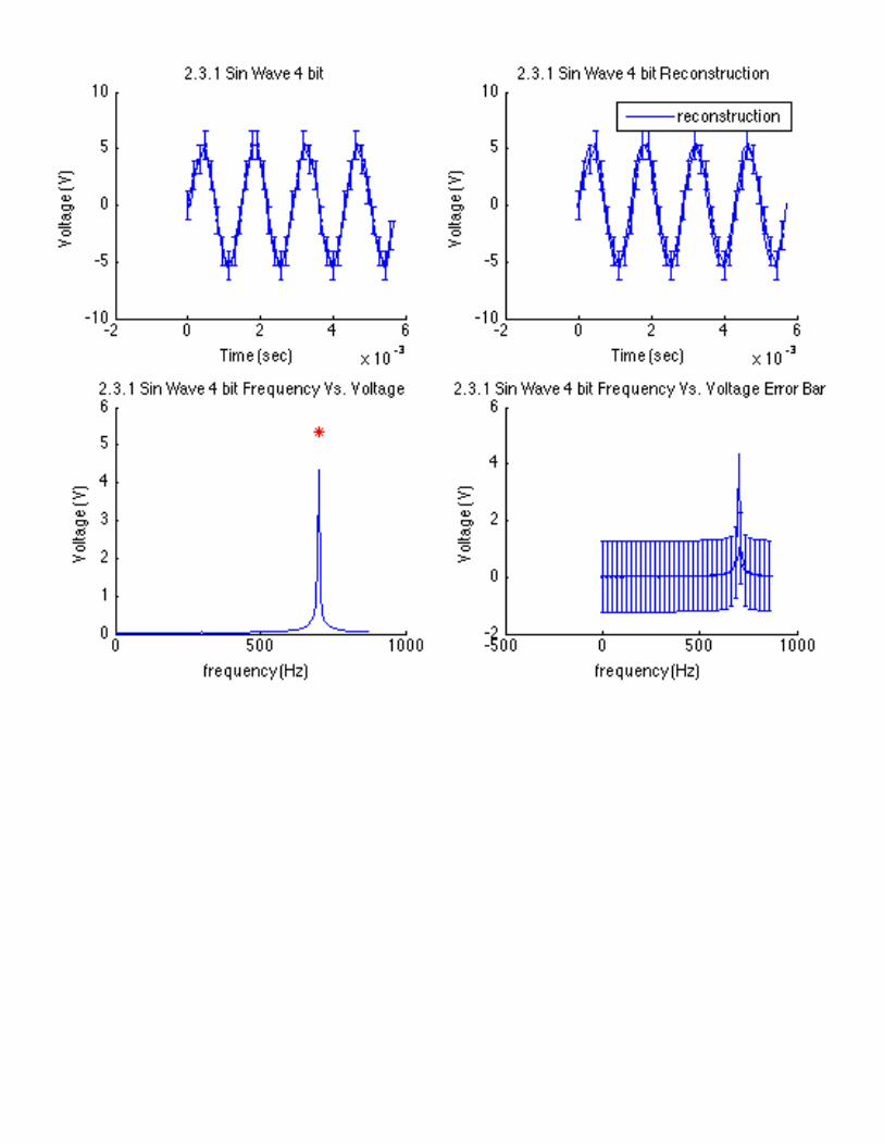
Otherkeyaspectswecontrolledinthissimulationtoachievetheseresultswere,numberofsamples,4096,bitresolution,12,andbipolarrange,+or–10volts.Thebitresolutioneffectshowsmooththesinwavecurvecomesout.Inthelabwetestedchangingthebitresolutionlowerandtheoutcomeswasthegraphonthenextpage,thegraphwaslessofasinwaveandmorelikeatrianglewave.Ifyouweretoincreasethebitresolutionpast12therewaslittletonochangeintheappearanceofthegraph.

Lee27

(Graph2)

Inthefrequencydomainongraph1weseeonlyonefrequencyat700Hz,whichisthesameasthefrequencyweinputted.Thisisthetruefrequencyofthewave.ApplyingNyquist’stheorem,whichstatesthatthesamplingfrequencymustbetwicethemaximumfrequency,wecheckthesamplingfrequency,25kHz,andthemaximumfrequencyofthesinwave,700Hz,andcompare.Thelowestsamplingfrequencythatcanbeusedforthisparticularcasesothatwepreventaliasingis1400Hzandanythinglowerwillbemisinterpreted.

(Graph3)

Lee28

TheNyquistfoldingdiagramillustratesthisandsinceoursamplingfrequencyis25kHz,thesimulationcanhaveamaximumfrequencyanywhereuptothere.

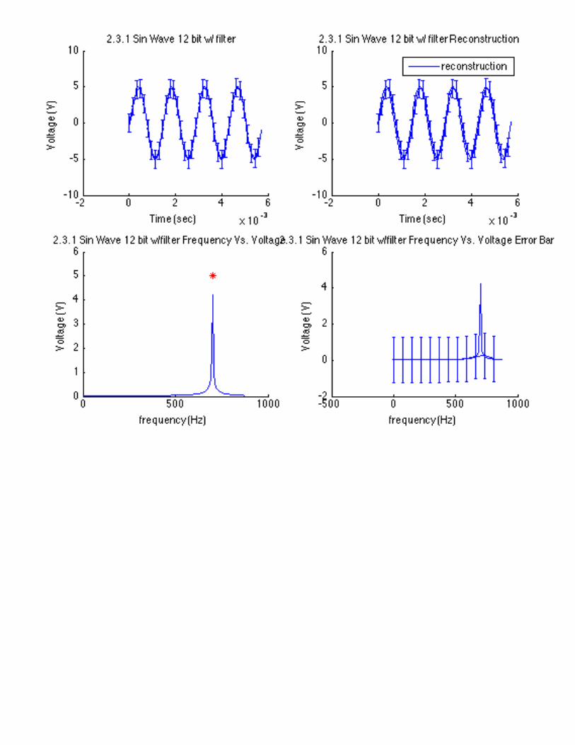
Nextwewillbeusingalowpassfilterwithacutoffofhalfonasquareandsawtoothwavewithanamplitudeof5voltswiththesamefrequencyandsamplingfrequencyastheprevioussimulation,700Hz,and25kHz.Comparingthesquarewavewithandwithoutthefilteronwecanseethatasmallportionofnoisewasremovedwhenthefilterwasactivated.(Graph4)

Lee29

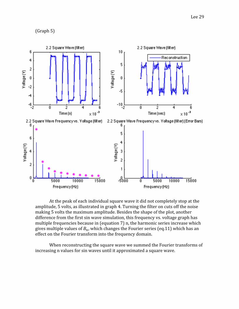
(Graph5)

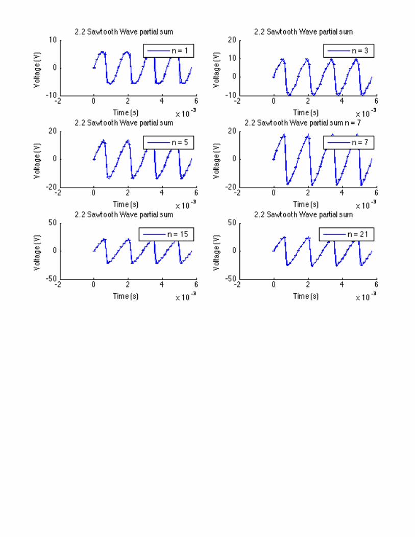
Atthepeakofeachindividualsquarewaveitdidnotcompletelystopattheamplitude,5volts,asillustratedingraph4.Turningthefilteroncutsoffthenoisemaking5voltsthemaximumamplitude.Besidestheshapeoftheplot,anotherdifferencefromthefirstsinwavesimulation,thisfrequencyvs.voltagegraphhasmultiplefrequenciesbecausein(equation7)n,theharmonicseriesincreasewhichgivesmultiplevaluesof𝐵!,whichchangestheFourierseries(eq.11)whichhasaneffectontheFouriertransformintothefrequencydomain. WhenreconstructingthesquarewavewesummedtheFouriertransformsofincreasingnvaluesforsinwavesuntilitapproximatedasquarewave.

Lee30

(Graph6)

Atn=1itisastandardsinwavewiththesameamplitudeasthesquare

wave.Asnincreasestheshapemoreorlesslookslikethesquarewavewesimulated. Similarly,thesawtoothfunctionhadanamplitudeof5voltsbutrangedfrom+5to-5volts(Graph7).Thefrequenciesatwhichresultedwithpeakssteppedby700Hzwherethesquarewavewentstartedat700Hzbutsteppedby1400Hz.AgainneitherthesawtoothnorthesquarewavewerealiasedifyoulookattheNyquistfoldingdiagram(Graph8)and(Graph9).Thedatacollectedcomplieswiththetheoryandnothingdeviatedtoalarmusthatsomethinghadgonewrong.

Uncertaintyinthesimulationwasduetoequipmentusedtosimulatethefunctionsandtheparameters,whichweusedinthisexperiment.Theuncertaintyinvoltagewascalculatedusing(eq.26)withaN=13,bi-polarrangeof+/-10voltsthendividingitbyonehalf.Butifweweretoimprovethetime,voltageandfrequencyresolutionwewouldseeouruncertaintydecreasegivingamoreexactapproximationofthetheory.

Lee31

(Graph7)

(Graph8)

Lee32

(Graph9)

Thesecondpartinthissectionwastotakethefilteroffofthesawtoothwaveandseewhateffectsithad,howeverwhenanalyzingthegraphs,(graph10)therewerenotanydifferences.(Graph10)

Lee33

Anotherproblemthatmaycomealongisclipping.Clippingiswhenthesignaliscutoffatacertainpoint.Wesimulatedaclippedsignalwithasinwaveusingthesamesettingsinthefirstsectionexceptchangingthebipolarvoltageto+/-1volt.Changingbipolarvoltagechangesthevoltageresolutionandtheuncertaintyintheamplitudeofthesignal.(Graph11)

Asyoucanseebythepeaksofthesinwavebeingclipped,thesignalshouldhaveaamplitudeof5voltsandlookexactlylikethevoltagevs.timeplotingraph1.Thiscouldposeaproblemifusedinanapplication.Ifthevoltageresolutionistolow,whenthesignalisprocesseditwillbemisinterpretedwithaincorrectamplitude.Thecharacteristicofthewaveformbecomesdistorted.TheNyquistfoldingdiagram,(Graph12)isidenticaltotheunclippedsinwave.Sotheonlychangewhenthebipolarvoltageisdroppedisthevoltageinthetimedomain.

Lee34

Forexample,inaspeechrecognitiondevicewhereitprocessesanalogsignals,voices,ifthesignalisbeingclippedduringthesignalconditioningitcanleadtothedeviceincorrectlyinterpretingthesignalandgivingwrongcommands. (Graph12)

Intherestofthelabwedidnotusesimulationstotestthetheorybutactualexperiments.ActualfunctiongeneratorsandfilterswereusedtocreatethesignalandthenpassitintoLABVIEW.Thefirstexperimentinvolvedasinwavegeneratingafrequencyof700Hzandaamplitudeof3.8V,itwasofffromthepreset5Vpriortotheourlabsection.Wethenselectedasamplingfrequencyof25kHzandnumberofsamplesto8192.In(graph13)westilldonotencounteraliasingbecausethesamplingfrequencyisstillfargreaterthanthemaximumfrequencyofthesignal,700Hz,andtheNyquistfoldingdiagramagainillustratesthis.Thefrequencywassetto700Hzand700Hziswhatwesee.Ifitwasaliaseditwouldhavechanged.

Lee35

(Graph13)

(Graph14)

Lee36

ToexperimentwithaliasingandfilteringinthispartofthelabwerepeatedthepreviousprocesswiththesinwavebutwithasamplingfrequencythatisdoesnotfollowNyquistTheorem,wesetitto1000Hz.(Graph15)

Wenowseealiasing,weknowthisbecausethefrequencyofthesignalisstill700Hz,butwearenowseeingaroundthefrequencytobearound290Hz.Inthetimevs.voltagegraphwealsodonotseeasmoothsinwave,whichgivesusasuspicionthatsomethingiswrong.TheNyquistfoldingdiagramillustrateshowthefrequencyfoldeddownfromthetruefrequencytowhatitappearsnowas(Graph16).

Lee37

(Graph16)

WethentriedtocorrectthisaliasingproblembyapplyingaKrohn-Hitefiltertothesamesignal.(Graph17)

Lee38

(Graph18)

WeobservedthatapplyingtheKrohn-Hitefiltercouldsolvetheproblemofaliasingandtosolveityouwouldhavetoupthesamplingfrequencyofthesignal.

Aliasingoccursinmultiplerealworldapplicationslikephotography.In

digitalphotography,aliasingoccurswiththequalityofpictures.Thisisduetotheresolutionofthecamerabeingused.Whenapictureistakentheanaloglightandcolorthatweseeinthephysicalworldisconvertedtoadigitalsignalbyhavinglightenterthroughthelensofthecameraandhittingasensor.Thatsensorconvertsthelightandcolorintopixels.Themorepixelsthatthesensorhasthesharperandmoreclearthepicturebecomes,howeveriftheresolutionofthecameraistolowyouwillbeabletoseethediscontinuitiesincoloranddistortionbetweeneachpixel. Alldigitalcamerashavesomedegreeofaliasing(AutumnLockwood,1);thesmallersensorcamerasaliasmoreandthiscanbeexaggeratedwhenthepicturesizeisincreased.Incrimemovieswhenthepolicespotasuspiciouscarandneedtozoominonthelicenseplate,thecamerawiththebiggersensorwillbeabletokeepthepictureatahigherresolutionthanacamerawithalowerresolution.Howeverthedegreetowhichmoviesexaggeratethiswhentheyzoomin5timesandthepictureisstillcrystalclearisridiculous.

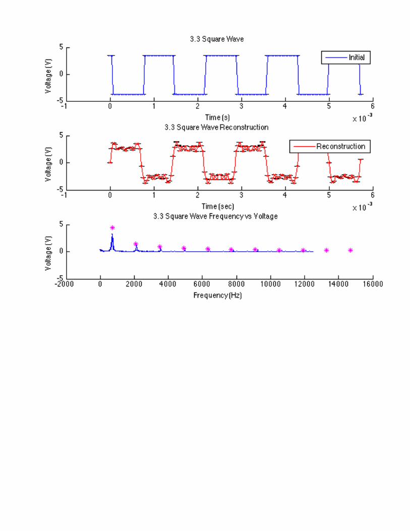
Comparingoursimulationtotheorywefoundthatitmatched.Butnowcomparinganexperimenttobothsimulationandtheorywechoseasquarewaveat700Hzanda25kHzsamplerate.PlottingthedataitdoesmatchthetheoryandreconstructingthegraphwithFourieranalysiswecanseearoughreconstructionofthesquarewave.(Graph19)

Lee39

(Graph19)

Theamplitudeonthevoltagevs.timegraphwas3.8volts,becauseitwasnot

initially5volts,andagainmatchesthetheoryandsimulation.Boththepartialreconstructions(Graph21)andtheNyquistfoldingdiagram(Graph20)replicatethesimulateddataplotsbeforeandmatchesthetheory. Thiswasalsodoneforasawtoothfunctionwiththesameconstraints.Theplotsreplicatethesimulationdata.(Graph22,23,24)

Lee40

(Graph20)

(Graph21)

Lee41

(Graph22)

(Graph23)

Lee42

(Graph24)

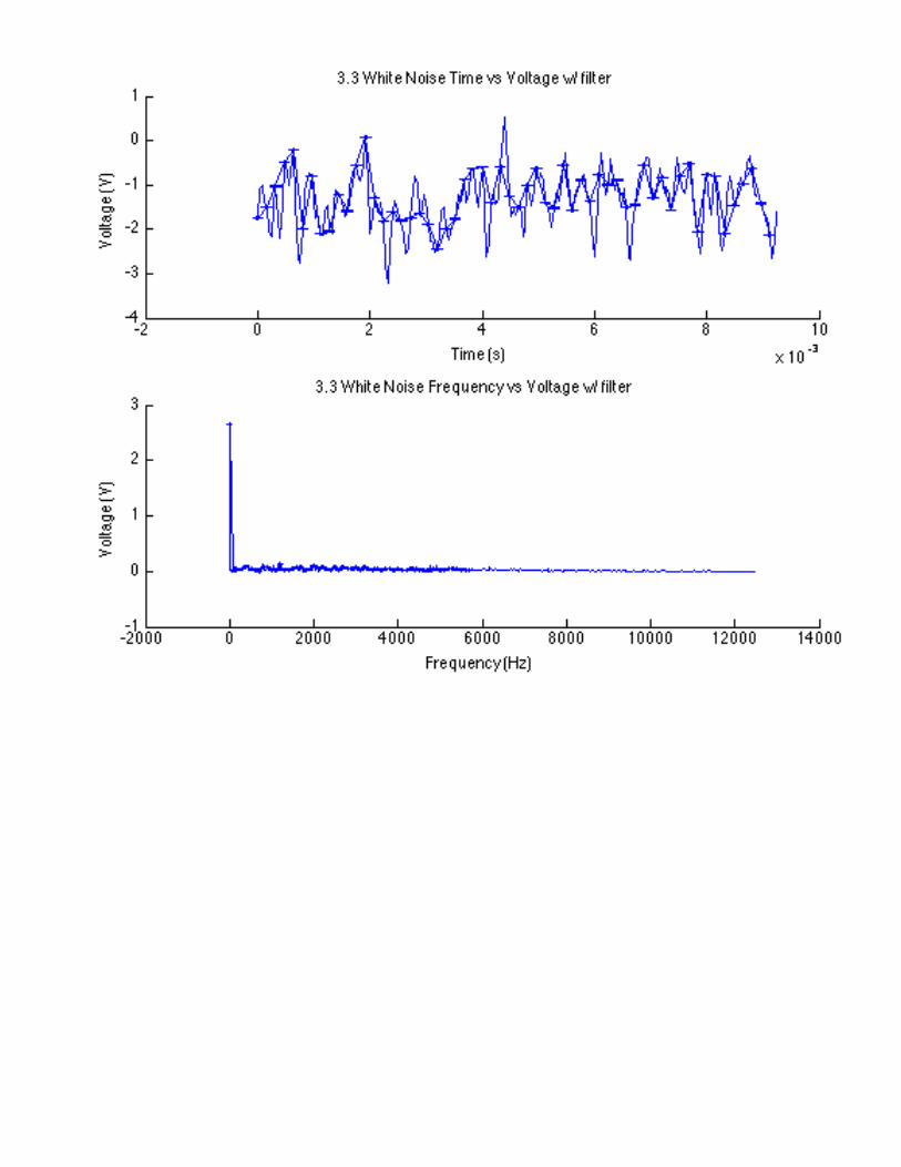
Finallyweexperimentedwithwhitenoisewiththehighestsampling

frequencywecoulduse,40kHz,withalowpassfiltertopreventaliasing.Lookinginthefrequencydomainwecanseetheslowdecay,from2Hzto20kHz,inthefrequencyseries,meaningthatitwasapoorfilter.

Lee43

(Graph25)

ResultsinVibrationslab First,weexperimentedwiththebeamsresponsewithashaker.Weinputtedthecorrectinputfrequencyandrecordeddidasweepacrosstherangeoffrequenciestryingtodiscernwherethemaximumdisplacementoftheendofthebeamwas.Weestimatedthe17-inchbeamtesttobearound26Hz,the19-inchbeamat19Hz,andthe22-inchbeamat16Hz.Thenplottingthedata,graph26,wewereprettycloseinourestimationbyfindingeachindividualpeakontheamplitudevs.frequencyplots.Alsobylookingattable1(page151)intheappendixweconfirmourassumptions.

Lee44

(Graph26)

Thesefrequenciesatwhichwesawmaximumdeflectioninthebeamareconsideredthenaturalfrequencyofthesystemandiswhatyoudonotwantthestructuretoencounterinarealworldapplicationbecauseitwillleadtofailure.Theuncertaintyweseeisduetothesamplingfrequencyand#ofsamples. Next,weexperimentedwithanimpulse.Weappliedaforcewithahammerontotheendofthebeam.Wewereabletocapturetheinputandoutputresponsebyhavinganaccelerometeronthetipofthehammeraswellastheedgeofthebeam.Weplottedthedatatofindtheamplitudevs.timeoftheinputandoutput.Weseeaunderdampedsinusoidalwaveformthathasthemaximumdeltaasthehammerinitiallymakescontactwiththebeamasyoucanseeingraph27.Theexperimentalfrequencywegotforthebeamatalengthof17,19,and22were26Hz,21Hz,and16Hz(graph28).Akeyfactorthatvarieseachtestwashowthehammerimpactedthebeam.Factorslike,wasthehammerimpactperpendiculartothebeam,didthebeamreboundandstrikethehammeragaincausingmultipleimpactstohappen,etc.Beingthatthiswasanexperiment,theuncertaintyincertainvariablesmaycausetheresultstonotidenticallymatchthetheory.

Lee45

(Graph27)

TheMagnitudeofResponsewascalculatedbyfindingusingeq.24,25and

FFT,fortherealandimaginarypartsofthefunction,inMATLABthenplottingtheinputandoutput.Fourierallowedustomodelanunknownsignal,whichwedidn’tknowthemathematicalsolutionasonewherewealreadyknowthesolution.Wemodeleditasaspringmassdampedsystemandfoundtheresulttoit.Phaselagwascalculatedandplottedtogiveasenseofhowthebeamresonatedinandoutofphaseacrosstherangeoffrequencies.Theinputwentfromaround160degreesto-160degreesandtheoutputfrom49degreesto-149degrees.(Graph31)

Lee46

(Graph28)

(Graph29)

Lee47

(Graph30)

(Graph31)

Lee48

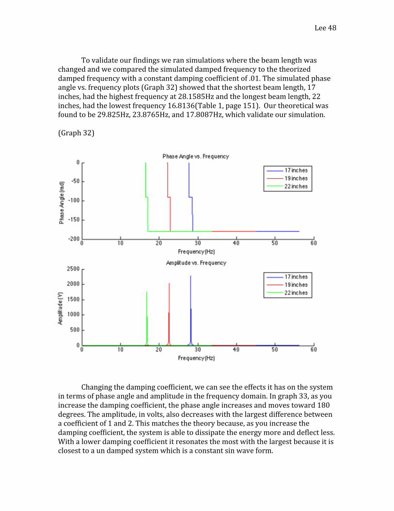
Tovalidateourfindingsweransimulationswherethebeamlengthwaschangedandwecomparedthesimulateddampedfrequencytothetheorizeddampedfrequencywithaconstantdampingcoefficientof.01.Thesimulatedphaseanglevs.frequencyplots(Graph32)showedthattheshortestbeamlength,17inches,hadthehighestfrequencyat28.1585Hzandthelongestbeamlength,22inches,hadthelowestfrequency16.8136(Table1,page151).Ourtheoreticalwasfoundtobe29.825Hz,23.8765Hz,and17.8087Hz,whichvalidateoursimulation.(Graph32)

Changingthedampingcoefficient,wecanseetheeffectsithasonthesystemintermsofphaseangleandamplitudeinthefrequencydomain.Ingraph33,asyouincreasethedampingcoefficient,thephaseangleincreasesandmovestoward180degrees.Theamplitude,involts,alsodecreaseswiththelargestdifferencebetweenacoefficientof1and2.Thismatchesthetheorybecause,asyouincreasethedampingcoefficient,thesystemisabletodissipatetheenergymoreanddeflectless.Withalowerdampingcoefficientitresonatesthemostwiththelargestbecauseitisclosesttoaundampedsystemwhichisaconstantsinwaveform.

Lee49

(Graph33)

Thematerialofthebeaminthissimulationwascarbonsteelandthebeamslengthwaskeptconstantat22inchesforeverytest.Ifwelookbacktothehammertest,ifthecoefficientofdampingwaslarger,theamplitudeoftheresponsewouldbeexponentiallylowerthanifthebeamhadasmalldampingcoefficient.Ineq.16weseehowtheeffectsofC,thedampingcoefficientpropagatethroughtheequationsstartingwithwhatkindofsystemitisbasedonthevalueofzeta.Thenzetaisusedtofindtheresonancefrequency(eq.26)anddampednaturalfrequency(eq.15). Inthezetaratio(eq.16)thematerialsmassalsofactorsintowhetheritisoverdamped,underdamped,criticallydamped,orun-damped.Ifthedampingcoefficientyouareworkingwithishigh,youwouldwanttodecreasethemasssothatthedampingratiozetaisoverdampedandthedeflectionisminimized. Theeffectsofendmassingraph34showthatasweightincreasesthedampedfrequencydecreases.Wetestedthiswith3differentmassesandthisbacks

Lee50

thetheoryup.Asstatedbefore,thenaturalfrequencydependsonzetaandasyouincreasemassthezetashrinks.Thisinturnlowersthedampednaturalfrequency.(Graph34)

Nowifthematerialtypechangeswhichchangesthestiffnesscharacteristicsofthebeam,byachangeinYoung’sModulus,thenthenaturalfrequencychanges.Justlikedesigningabuildingandchoosingthecorrectmaterialthathastherightductility,strength,hardness,etc.,theengineerhastolookathowthatmaterialrespondstovibrationsandwhatfrequenciesthesystemdealswith.

Conductingthesetypesofvibrationstestscaneducateengineersonhowtodesignstructurestowithstandcertainforces.Whetherit’samotorvehicledrivingonunevenroad,bridges,buildings,oreverydaydevicesweuse.Ifitisnotaccountedforvibrationscanleadtounbalance,misalignment,loosening,bearingwear,resonance,andothertypesoffailure.

Lee51

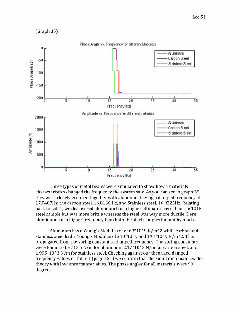
(Graph35)

Threetypesofmetalbeamsweresimulatedtoshowhowamaterialscharacteristicschangedthefrequencythesystemsaw.Asyoucanseeingraph35theywerecloselygroupedtogetherwithaluminumhavingadampedfrequencyof17.0407Hz,thecarbonsteel,16.8136Hz,andStainlesssteel,16.9225Hz.RelatingbacktoLab1,wediscoveredaluminumhadahigherultimatestressthanthe1018steelsamplebutwasmorebrittlewhereasthesteelwaswaymoreductile.Herealuminumhadahigherfrequencythanboththesteelsamplesbutnotbymuch. AluminumhasaYoung’sModulusofof69*10^9N/m^2whilecarbonandstainlesssteelhadaYoung’sModulusof210*10^9and193*10^9N/m^2.Thispropagatedfromthespringconstanttodampedfrequency.Thespringconstantswerefoundtobe713.5N/mforaluminum,2.17*10^3N/mforcarbonsteel,and1.995*10^3N/mforstainlesssteel.CheckingagainstourtheorizeddampedfrequencyvaluesinTable1(page151)weconfirmthatthesimulationmatchesthetheorywithlowuncertaintyvalues.Thephaseanglesforallmaterialswere90degrees.

Lee52

Conclusion Thesimulatedfunctionsweren’taliasedbecausethe½xsamplingfrequencywasstillhigherthanthemaximumfrequencyofthefunctionanditnevercameclosetothepointatwhichthesignalwouldbealiased.Ifwewerenotgiventhemaximumfrequencyofthesignalwecouldusealowpassfilterwhichblocksouteverythingafterthecutoffandonlyallowsthefrequencyuptothecutofftopass.Youcouldthenmovethelowpassfilterfurtherandfurtherorincreasethesamplingfrequencyuntilyoucansafelyassumethatthefrequencyyouaregettinginyourresultsisthattruefrequencyofthesignal. Ifweweretoplotthefrequencyspectrumofwhitenoisewithasamplefrequencyof25kHzandabandpassfilterfrom5kHzto20kHzwewouldseesomethingsimilartofigure4with5kHzbeingthehighpassand20kHzbeingthelowpassfilter. Correctlyprocessingananalogsignaliscrucialtodevelopingsystemsthatcanaccuratelyconvertittoadigitalsignalsothatitcaneitherbeusedtoprogramsomethingorbeusedasdatawhenanalyzingananalogsystem.DSPisresponsibleformorethingstoworkthanweknow,listeningtomusic,communicatingthroughelectronicdevices,analyzingtheresponseofasystemunderdifferentcircumstanceslikethevibrationsportioninthislab,andevendigitallyprocessinganimage.

Accuratelymeasuringtheanalogsignalsandconvertingthemtodigitalsignalsiskeybecausethatmeanswecandesignstructuresinmanyapplicationstoabsorbanddissipateenergyortonotfailduetoresonatingatitsnaturalfrequency.

Inthevibrationslabwevalidatedourexperimentwithsimulationand

provedthateverythinghasanaturalfrequencythatitresonatesat.Weshowedthemanyfactorsthatinfluencetheoutcome.Thosefactorsinclude,geometryofthebeam,material,length,andmaterialproperty.

References

Beer,FerdinandP,ER.Johnston,andJohnT.DeWolf.MechanicsofMaterials.NewYork:McGraw-Hill,1992.Print.

(Fig.7)Scavone,GaryP.,editor."VibratingSystems."StandfordUniversity,CCRMA,ccrma.stanford.edu/CCRMA/Courses/150/vibrating_systems.html.

Lee53

(PictureCorrect)http://www.picturecorrect.com/tips/aliasing-in-digital-photography-explained/WilliamHarris"HowEarthquake-resistantBuildingsWork"13September2011.HowStuffWorks.com.<http://science.howstuffworks.com/engineering/structural/earthquake-resistant-buildings.htm>11November2016(UniversityWashington)http://www.lib.washington.edu/specialcollections/collections/exhibits/tnb(Glauser)http://ecs.syr.edu/faculty/glauser/mae315/

Appendix

DigitalSignalProcessingFourierDerivationsSinWaveFourierCoefficients

𝑎! =1𝑇 5sin (2𝜋𝑓!𝑡)

!

!𝑑𝑡

=5𝑇 (− cos 2𝜋𝑓!𝑡

2𝜋𝑓!|!!)

= −52𝜋 +

52𝜋

Lee54

𝑎! = 0

𝑎! =2𝑇 5sin (2𝜋𝑓!𝑡)cos (2𝜋𝑓!𝑡𝑛)

!

!𝑑𝑡

10𝑇 sin (2𝜋𝑓!𝑡)cos (2𝜋𝑓!𝑡𝑛)

!

!𝑑𝑡

𝐼 = 𝑠in (2𝜋𝑓!𝑡)cos (2𝜋𝑓!𝑡𝑛)

𝑢 = cos (2𝜋𝑓!𝑡𝑛)

dv = sin (2𝜋𝑓!𝑡)𝑑𝑡

du = −sin (2𝜋𝑓!𝑡𝑛)

2𝜋𝑓!𝑛𝑑𝑡

𝑣 = −cos(2𝜋𝑓!𝑡)

2𝜋𝑓!

= uv− 𝑣𝑑𝑢

𝐼 = −cos 2𝜋𝑓!𝑡 cos 2𝜋𝑓!𝑡𝑛

2𝜋𝑓!−

14𝜋!𝑓!

!𝑛cos 2𝜋𝑓!𝑡 sin 2𝜋𝑓!𝑡𝑛 𝑑𝑡

𝐽 = cos 2𝜋𝑓!𝑡 sin 2𝜋𝑓!𝑡𝑛 𝑑𝑡

𝑢 = sin 2𝜋𝑓!𝑡𝑛 𝑑𝑢 =cos (2𝜋𝑓!𝑡𝑛)

2𝜋𝑓!𝑛 𝑑𝑡

𝑣 = sin(2𝜋𝑓!𝑡)2𝜋𝑓!𝑡

𝑑𝑣 = cos 2𝜋𝑓!𝑡 𝑑𝑡

𝐽 = sin(2𝜋𝑓!𝑡𝑛)sin(2𝜋𝑓!𝑡)

2𝜋𝑓!𝑡−

14𝜋!𝑓!

!𝑛sin 2𝜋𝑓!𝑡 cos 2𝜋𝑓!𝑡𝑛 𝑑𝑡

Lee55

𝐽 = sin(2𝜋𝑓!𝑡𝑛)sin(2𝜋𝑓!𝑡)

2𝜋𝑓!𝑡−

14𝜋!𝑓!

!𝑛𝐼

= −cos 2𝜋𝑓!𝑡 cos 2𝜋𝑓!𝑡𝑛

2𝜋𝑓!−

14𝜋!𝑓!

!𝑛(sin 2𝜋𝑓!𝑡𝑛 sin 2𝜋𝑓!𝑡

2𝜋𝑓!−

14𝜋!𝑓!

!𝑛𝐼)

= −cos 2𝜋𝑓!𝑡 cos 2𝜋𝑓!𝑡𝑛

2𝜋𝑓!−sin 2𝜋𝑓!𝑡𝑛 sin 2𝜋𝑓!𝑡

8𝜋!𝑓!!𝑛

+1

16𝜋!𝑓!!𝑛!

𝐼

𝐼 = 8𝜋!𝑓!

!𝑛! cos 2𝜋𝑓!𝑡 cos 2𝜋𝑓!𝑡𝑛 + 2𝜋𝑓!𝑛 sin 2𝜋𝑓!𝑡𝑛 sin 2𝜋𝑓!𝑡

=10𝑇 [8𝜋!𝑓!

!𝑛! cos 2𝜋𝑓!𝑡 cos 2𝜋𝑓!𝑡𝑛 + 2𝜋𝑓!𝑛 sin 2𝜋𝑓!𝑡𝑛 sin 2𝜋𝑓!𝑡 |𝑇0]

10𝑇 8𝜋!𝑓!

!𝑛! − 8𝜋!𝑓!!𝑛! = 0

𝑎! = 0

𝑏! = 2𝑇 5 sin 2𝜋𝑓!𝑡 sin 2𝜋𝑓!𝑡𝑛

!

!𝑑𝑡

n=1

=10𝑇

1− cos (4𝜋𝑓!𝑡)2

!

!𝑑𝑡

=10𝑇 [

12 𝑡 −

sin 4𝜋𝑓!𝑡2 |!!]

= 5− 0𝐵! = 5

SquareWaveFourierCoefficients

𝑎! =1𝑇 5 𝑑𝑡 +

1𝑇 −5 𝑑𝑡

!

!!/!

!/!

!

𝑎! =52− (5−

52)

𝑎! = 0

Lee56

𝑎! =2𝑇 5cos (2𝜋𝑓!𝑡𝑛)

!/!

!𝑑𝑡 +

2𝑇 −5cos (2𝜋𝑓!𝑡𝑛)

!

!/!𝑑𝑡

= [10𝑇 (

𝑠𝑖𝑛 2𝜋𝑓!𝑡𝑛2𝜋𝑓!𝑛

|!!!]+ [

−10𝑇 (

𝑠𝑖𝑛 2𝜋𝑓!𝑡𝑛2𝜋𝑓!𝑛

|!!

!]

=10sin (𝜋𝑛)

𝜋𝑛 −5sin (2𝜋𝑛)

𝜋𝑛

𝑎! = 0 ,𝑛 = 1,2,3,… ,21

𝐵! =2𝑇 5𝑠𝑖𝑛 2𝜋𝑓!𝑡𝑛 𝑑𝑡 +

2𝑇 −5𝑠𝑖𝑛 2𝜋𝑓!𝑡𝑛 𝑑𝑡

!

!!/!

!/!

!

= [10𝑇 (−

𝑐𝑜𝑠 2𝜋𝑓!𝑡𝑛2𝜋𝑓!𝑛

|!!!]+ [

−10𝑇 (−

𝑐𝑜𝑠 2𝜋𝑓!𝑡𝑛2𝜋𝑓!𝑛

|!!

!]

𝐵! = −10 cos 𝜋𝑛

𝜋𝑛 +5cos (2𝜋𝑛)

𝜋𝑛 SawtoothWaveFourierCoefficients(A=amplitude)

𝑎! =1𝑇

2𝐴𝑡𝑇 𝑑𝑡

!/!

!!/!

=2𝐴𝑇! (

𝑡!

2 |!!!

!! )

𝑎! = 0

Lee57

𝑎! = 2𝑇

2𝐴𝑡𝑇 cos (2𝜋𝑓!𝑡𝑛)

!/!

!!/!𝑑𝑡

𝑢 =2𝐴𝑡𝑇 𝑑𝑢 =

2𝐴𝑇 𝑑𝑡

𝑣 = sin (2𝜋𝑓!𝑡𝑛)

2𝜋𝑓!𝑛 𝑑𝑣 = 𝑐 os 2𝜋𝑓!𝑡𝑛 𝑑𝑡

=Atsin(2𝜋𝑓!𝑡𝑛)

𝜋𝑛 −𝐴𝜋𝑛 sin 2𝜋𝑓!𝑡𝑛 𝑑𝑡

=2𝑇 [Atsin 2𝜋𝑓!𝑡𝑛

𝜋𝑛 +𝐴 cos 2𝜋𝑓!𝑡𝑛2𝜋!𝑛!𝑓!

|!!!

!! ]

𝑎! = 0

𝑏! = 2𝑇

2𝐴𝑡𝑇 sin (2𝜋𝑓!𝑡𝑛)

!/!

!!/!𝑑𝑡

𝑢 =2𝐴𝑡𝑇 𝑑𝑢 =

2𝐴𝑇 𝑑𝑡

𝑣 = −cos(2𝜋𝑓!𝑡𝑛)2𝜋𝑓!𝑛

𝑑𝑣 = sin 2𝜋𝑓!𝑡𝑛 𝑑𝑡

= −Atcos(2𝜋𝑓!𝑡𝑛)

𝜋𝑛 −𝐴𝜋𝑛 −cos 2𝜋𝑓!𝑡𝑛 𝑑𝑡

=2𝑇 [−

Atcos 2𝜋𝑓!𝑡𝑛𝜋𝑛 +

𝐴 sin 2𝜋𝑓!𝑡𝑛2𝜋!𝑛!𝑓!

|!!!

!! ]

𝑏! = −2𝐴 cos 𝜋𝑛

𝜋𝑛

Lee58

Table2TableofCoefficients

SquareWave

n= An Bn Amplitude(volts)

1 0 6.366 3.7448

2 0 0 3.7448

3 0 2.122 3.7448

4 0 0 3.7448

SawToothWave

n= An Bn Amplitude(volts)

1 0 3.183 3.7448

2 0 -1.592 3.7448

3 0 1.061 3.7448

4 0 -0.796 3.7448

Lee59

NyquistPlots2.1SinewaveNyquistPlot

2.2Sawtooth(filter)NyquistPlot

12500Hz

25000Hz37500Hz

50000Hz 62500Hz

0Hz

12500Hz

25000Hz37500Hz

50000Hz 62500Hz

0Hz

700Hz

700Hz 1400Hz 2100Hz 2800Hz

Lee60

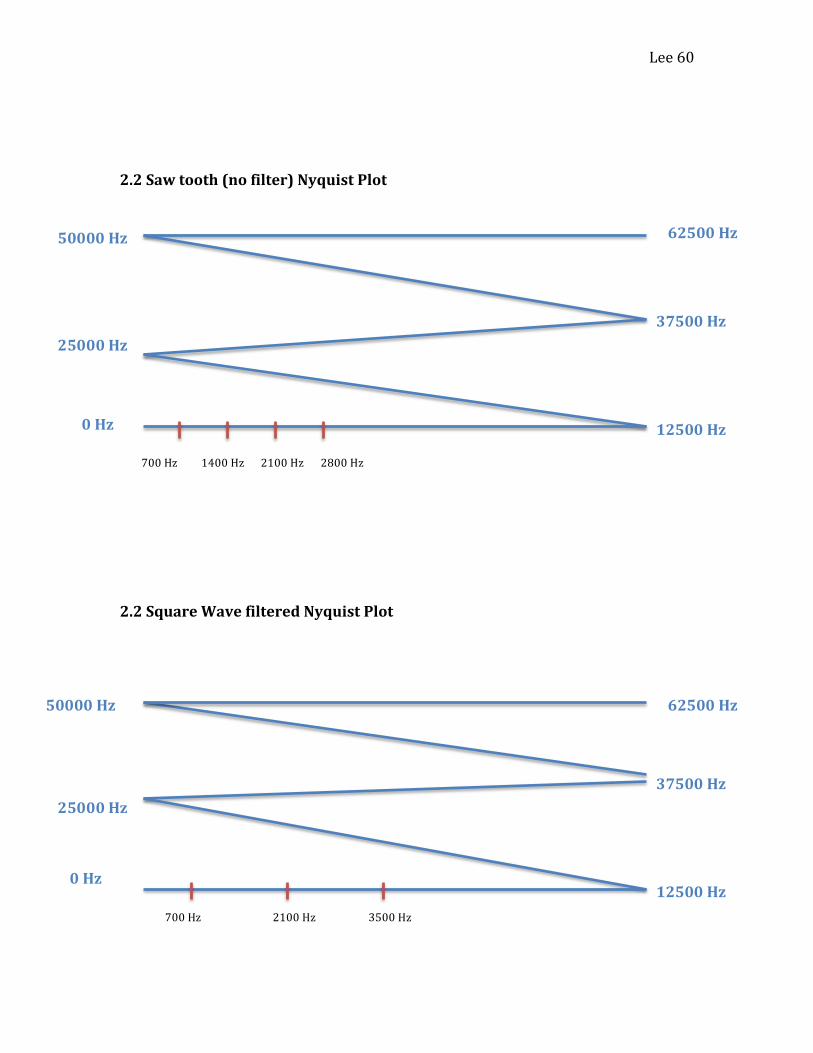
2.2Sawtooth(nofilter)NyquistPlot

2.2SquareWavefilteredNyquistPlot

12500Hz

25000Hz37500Hz

50000Hz 62500Hz

0Hz

12500Hz

25000Hz37500Hz

50000Hz 62500Hz

0Hz

700Hz 1400Hz 2100Hz 2800Hz

700Hz 2100Hz 3500Hz

Lee61

2.2SquarenofilterNyquistPlot

2.3.1SineWave(4Bit)NyquistPlot

12500Hz

25000Hz37500Hz

50000Hz 62500Hz

0Hz

12500Hz

25000Hz37500Hz

50000Hz 62500Hz

0Hz

700Hz 2100Hz 3500Hz

700Hz700Hz

Lee62

2.3.1SinWave(12Bit)w/FilterNyquistPlot

2.3.2ClippedSineWaveNyquistPlot(+/-10volts)

12500Hz

25000Hz37500Hz

50000Hz62500Hz

0Hz

12500Hz

25000Hz37500Hz

50000Hz 62500Hz

0Hz700Hz

700Hz

Lee63

2.3.2ClippedSineWaveNyquistPlot(+/-1volts)

3.1ExperimentalSinewaveNyquistPlot

12500Hz

25000Hz 37500Hz

50000Hz62500Hz

0Hz

12500Hz

25000Hz 37500Hz

50000Hz 62500Hz

0Hz

700Hz

700Hz

Lee64

3.2SinWave(1000Hzsamplefrequency)

3.2Krohn-HiteFilterNyquistPlot

500Hz

1000Hz1500Hz

2000Hz 2500Hz

0Hz

500Hz

1000Hz1500Hz

2000Hz 2500Hz

0Hz

290Hz

300Hz

700Hz

Lee65

3.3SquareWaveNyquistPlot

3.3SawToothNyquistPlot

12500Hz

25000Hz37500Hz

50000Hz 62500Hz

0Hz

12500Hz

25000Hz37500Hz

50000Hz 62500Hz

0Hz

700Hz 2100Hz 3500Hz

700Hz 1400Hz 2100Hz 2800Hz

Lee66

Plots

Lee67

Lee68

Lee69

Lee70

Lee71

Lee72

Lee73

Lee74

Lee75

Lee76

Lee77

Lee78

Lee79

Lee80

Lee81

Lee82

Lee83

Lee84

Lee85

Lee86

Lee87

Matlab Code clear all; close all 2.1 Sin Wave Fourier Series Coefficients syms P n amp time xt = amp*sin(2*pi*time/P); Ani = xt*cos(2*n*pi*time/P); Bni = xt*sin(2*n*pi*time/P); A0 = (2/P)*int(xt,time,-P/2,P/2); An = (2/P)*int(Ani,time,-P/2,P/2); Bn = (2/P)*int(Bni,time,-P/2,P/2); Time vs Voltage s = importdata('10_4_2016lee2.1dat.txt'); data = s.data; time = data(:,1); % Seconds voltage = data(:,2); %Volts amp = 5; %Volts F = 700; %Hz P = 1/F; %Hz^-1 freq_samp = 25000; %Hz i = ceil(P*freq_samp); t = time(1:4*i); % seconds V = voltage(1:4*i); %Volts A0 = subs(A0); An = subs(An); Bn = subs(Bn); sum = 0; for n = 1:1; if n==1; B = amp; %Volts else B = Bn; end FFT = (A0/2)+(An*cos(2*n*pi*time/P)+B*sin(2*n*pi*time/P)); sum = sum + FFT; end % Uncertainty Vres = 20/(2^(13-1)); %Volts Tres = 1/(freq_samp); %seconds Fres = freq_samp/4096; %Hz u_volt = (Vres/2)*ones(1,length(t)); %Volts

Lee88

u_time = .5*(1/freq_samp)*ones(1,length(t)); %seconds Frequency vs. Voltage s = importdata('10_4_2016lee2.1fft.txt'); data = s.data; frequency = data(:,1); %Hz vf = data(:,2); %Volts amp_freq = max(vf); f = frequency(1:144); %Hz v_f = vf(1:144); %Volts %Uncertainty u_v_f = (Vres/2)*ones(1,length(v_f)); %Volts u_freq = (Fres/2)*ones(1,length(f)); % Hz u_v_f1 = u_v_f(1:144); %Volts u_f1 = u_freq(1:144); %Hz Plots figure(1) subplot(3,1,1) hold on plot(t,V) title('2.1 - Sin Wave') xlabel('Time (sec)') ylabel('Voltage (V)') errorbar(t(1:4:144),V(1:4:144),u_volt(1:4:144)) herrorbar(t(1:4:144),V(1:4:144),u_time(1:4:144)) legend('initial') subplot(3,1,2) hold on plot(t,V,t,sum(1:length(t))) title('2.1 - Sin Wave Reconstruction') xlabel('Time (sec)') ylabel('Voltage (V)') legend('Reconstruction') errorbar(t(1:4:144),V(1:4:144),u_volt(1:4:144)) herrorbar(t(1:4:144),V(1:4:144),u_time(1:4:144)) subplot(3,1,3) hold on plot(f,v_f,700,max(voltage),'r*') title('2.1 Frequency vs. Voltage Sin Wave') xlabel('Frequency (Hz)') ylabel('Voltage (V)') errorbar(f(1:4:144),v_f(1:4:144),u_v_f1(1:4:144)) herrorbar(f(1:4:144),v_f(1:4:144),u_f1(1:4:144))

Lee89

Nyquist fn = freq_samp/2; %Hz fn_2 = 2*fn; %Hz fn_3 = 3*fn; %Hz fn_4 = 4*fn; %Hz fn_5 = 5*fn; %Hz

Lee90

clear all; close all; 2.2 Fourier Analysis Square Wave (filter) % Square Wave Time vs Voltage a = importdata('10_4_2016lee2.2squarefilterdat.txt'); data = a.data; time = data(:,1); %Seconds voltage = data(:,2);%Volts amp = max(voltage); %Volts F = 700; %Hz P = 1/F; %Hz^-1 freq_samp = 25000; %Hz i = ceil(P*freq_samp); t = time(1:4*i); %Seconds V = voltage(1:4*i); %Volts %Uncertainty Vres = 20/(2^(13-1)); %Volts Tres = 1/(freq_samp); %Seconds Fres = freq_samp/4096; %Hz u_volt = (Vres/2)*ones(1,length(t)); %Volts u_time = .5*(1/freq_samp)*ones(1,length(t)); %Seconds % Square Wave Frequency vs. Voltage a = importdata('10_4_2016lee2.2squarefilterfft.txt'); data = a.data; frequency = data(:,1); %Hz vf = data(:,2); %Volts %Uncertainty u_v_f = (Vres/2)*ones(1,length(vf)); %Volts u_freq = (Fres/2)*ones(1,length(frequency)); %Hz Plots figure(1) subplot(2,2,1) plot(t,V,'b') hold on xlabel('Time (s)') ylabel('Voltage (V)') title ('2.2 Square Wave (filter)') errorbar(t(1:4:144),V(1:4:144),u_volt(1:4:144),'k') herrorbar(t(1:4:144),V(1:4:144),u_time(1:4:144),'b') subplot(2,2,2) sum = 0; A0 = 0; An = 0;

Lee91

for n = [1 3 5 7 15 21]; if n==1 B = amp; %Volts else B = (amp/(pi*n))*(1-(2*cos(pi*n))+(cos(2*pi*n))); %Volts end FFT = B*sin(2*n*pi*time/P); sum = sum + FFT; end hold on plot(t,sum(1:length(t))) title ('2.2 Square Wave (filter)') xlabel('Time (sec)') ylabel('Voltage (V)') legend('Reconstruction') errorbar(t(1:4:144),sum(1:4:144),u_volt(1:4:144),'k') herrorbar(t(1:4:144),sum(1:4:144),u_time(1:4:144),'b') subplot(2,2,3) hold on for w = 1:21 Bn(w) = (amp/(pi*w))*(1-(2*cos(pi*w))+(cos(2*pi*w))); %Volts end for e = 1:21 frq(e) = e * 700; %Hz end plot(frequency,vf,frq(1:2:end),Bn(1:2:end),'m*') xlabel('Frequency (Hz)') ylabel('Voltage (V)') title ('2.2 Square Wave Frequency vs. Voltage (filter)') subplot(2,2,4) hold on plot(frequency,vf) errorbar(frequency(1:4:144),vf(1:4:144),u_v_f(1:4:144),'k') herrorbar(frequency(1:4:144),vf(1:4:144),u_freq(1:4:144)) xlabel('Frequency (Hz)') ylabel('Voltage (V)') title ('2.2 Square Wave Frequency vs. Voltage (filter) (Error Bars)')

Lee92

Partial Sums Plots figure(2) hold on subplot(3,2,1) for n = [1]; if n==1 B = amp; %Volts else B = (amp/(pi*n))*(1-(2*cos(pi*n))+(cos(2*pi*n))); %Volts end FFT = B*sin(2*n*pi*time/P); sum = sum + FFT; hold on plot(t,sum(1:length(t)),'k') title ('Partial sums') xlabel('Time (sec)')

Lee93

ylabel('Voltage (V)') errorbar(t(1:4:144),sum(1:4:144),u_volt(1:4:144),'k') herrorbar(t(1:4:144),sum(1:4:144),u_time(1:4:144),'b') legend ('n=1') end subplot(3,2,2) for n = [3]; if n==1 B = amp; else B = (amp/(pi*n))*(1-(2*cos(pi*n))+(cos(2*pi*n))); end FFT = B*sin(2*n*pi*time/P); sum = sum + FFT; hold on plot(t,sum(1:length(t)),'k') title ('Partial sums') xlabel('Time (sec)') ylabel('Voltage (V)') errorbar(t(1:4:144),sum(1:4:144),u_volt(1:4:144),'k') herrorbar(t(1:4:144),sum(1:4:144),u_time(1:4:144),'b') legend ('n=3') end subplot(3,2,3) for n = [5]; if n==1 B = amp; else B = (amp/(pi*n))*(1-(2*cos(pi*n))+(cos(2*pi*n))); end FFT = B*sin(2*n*pi*time/P); sum = sum + FFT; hold on plot(t,sum(1:length(t)),'k') title ('Partial sums') xlabel('Time (sec)') ylabel('Voltage (V)') errorbar(t(1:4:144),sum(1:4:144),u_volt(1:4:144),'k') herrorbar(t(1:4:144),sum(1:4:144),u_time(1:4:144),'b') legend ('n=5')

Lee94

end hold on subplot(3,2,4) for n = [7]; if n==1 B = amp; else B = (amp/(pi*n))*(1-(2*cos(pi*n))+(cos(2*pi*n))); end FFT = B*sin(2*n*pi*time/P); sum = sum + FFT; hold on plot(t,sum(1:length(t)),'k') title ('Partial sums') xlabel('Time (sec)') ylabel('Voltage (V)') errorbar(t(1:4:144),sum(1:4:144),u_volt(1:4:144),'k') herrorbar(t(1:4:144),sum(1:4:144),u_time(1:4:144),'b') legend ('n=7') end subplot(3,2,5) for n = [15]; if n==1 B = amp; else B = (amp/(pi*n))*(1-(2*cos(pi*n))+(cos(2*pi*n))); end FFT = B*sin(2*n*pi*time/P); sum = sum + FFT; hold on plot(t,sum(1:length(t)),'k') title ('Partial sums') xlabel('Time (sec)') ylabel('Voltage (V)') errorbar(t(1:4:144),sum(1:4:144),u_volt(1:4:144),'k') herrorbar(t(1:4:144),sum(1:4:144),u_time(1:4:144),'b') legend ('n=15') end subplot(3,2,6) for n = [21]; if n==1

Lee95

B = amp; else B = (amp/(pi*n))*(1-(2*cos(pi*n))+(cos(2*pi*n))); end FFT = B*sin(2*n*pi*time/P); sum = sum + FFT; hold on plot(t,sum(1:length(t)),'k') title ('Partial sums') xlabel('Time (sec)') ylabel('Voltage (V)') errorbar(t(1:4:144),sum(1:4:144),u_volt(1:4:144),'k') herrorbar(t(1:4:144),sum(1:4:144),u_time(1:4:144),'b') legend ('n=21') end

Lee96

Nyquist fn = freq_samp/2; %Hz fn_2 = 2*fn; %Hz fn_3 = 3*fn; %Hz fn_4 = 4*fn; %Hz fn_5 = 5*fn; %Hz clear all; close all; 2.2 Fourier Analysis Square Wave (no filter) % Square Wave Time vs Voltage a = importdata('10_4_2016lee2.2squaredat.txt'); data = a.data; time = data(:,1); %Seconds voltage = data(:,2);%Volts amp = max(voltage); %Volts F = 700; %Hz P = 1/F; %Hz^-1 freq_samp = 25000; %Hz i = ceil(P*freq_samp); t = time(1:4*i); %Seconds V = voltage(1:4*i); %Volts %Uncertainty Vres = 20/(2^(13-1)); %Volts Tres = 1/(freq_samp); %Seconds Fres = freq_samp/4096; %Hz u_volt = (Vres/2)*ones(1,length(t)); %Volts u_time = .5*(1/freq_samp)*ones(1,length(t)); %Seconds % Square Wave Frequency vs. Voltage a = importdata('10_4_2016lee2.2squarefft.txt'); data = a.data; frequency = data(:,1); %Hz vf = data(:,2); %Volts %Uncertainty u_v_f = (Vres/2)*ones(1,length(vf)); %Volts u_freq = (Fres/2)*ones(1,length(frequency)); %Hz Plots figure(1) subplot(2,2,1) plot(t,V,'b') hold on xlabel('Time (s)')

Lee97

ylabel('Voltage (V)') title ('2.2 Square Wave (no filter)') errorbar(t(1:4:144),V(1:4:144),u_volt(1:4:144),'k') herrorbar(t(1:4:144),V(1:4:144),u_time(1:4:144),'b') subplot(2,2,2) sum = 0; A0 = 0; An = 0; for n = [1 3 5 7 15 21]; if n==1 B = amp; %Volts else B = (amp/(pi*n))*(1-(2*cos(pi*n))+(cos(2*pi*n))); %Volts end FFT = B*sin(2*n*pi*time/P); sum = sum + FFT; end hold on plot(t,sum(1:length(t))) title ('2.2 - Square Wave (no filter)') xlabel('Time (sec)') ylabel('Voltage (V)') legend('Reconstruction') errorbar(t(1:4:144),sum(1:4:144),u_volt(1:4:144),'k') herrorbar(t(1:4:144),sum(1:4:144),u_time(1:4:144),'b') subplot(2,2,3) hold on for w = 1:21 Bn(w) = (amp/(pi*w))*(1-(2*cos(pi*w))+(cos(2*pi*w))); %Volts end for e = 1:21 frq(e) = e * 700; %Hz end plot(frequency,vf,frq(1:2:end),Bn(1:2:end),'m*') xlabel('Frequency (Hz)') ylabel('Voltage (V)') title ('2.2 Square Wave Frequency vs. Voltage (no filter)') subplot(2,2,4) hold on plot(frequency,vf) errorbar(frequency(1:4:144),vf(1:4:144),u_v_f(1:4:144),'k') herrorbar(frequency(1:4:144),vf(1:4:144),u_freq(1:4:144))

Lee98

xlabel('Frequency (Hz)') ylabel('Voltage (V)') title ('2.2 Square Wave Frequency vs. Voltage (no filter) (Error Bars)')

Partial Sums Plots figure(2) hold on subplot(3,2,1) for n = [1]; if n==1 B = amp; %Volts else B = (amp/(pi*n))*(1-(2*cos(pi*n))+(cos(2*pi*n)));

Lee99

%Volts end FFT = B*sin(2*n*pi*time/P); sum = sum + FFT; hold on plot(t,sum(1:length(t)),'k') title ('Partial sums') xlabel('Time (sec)') ylabel('Voltage (V)') errorbar(t(1:4:144),sum(1:4:144),u_volt(1:4:144),'k') herrorbar(t(1:4:144),sum(1:4:144),u_time(1:4:144),'b') legend ('n=1') end subplot(3,2,2) for n = [3]; if n==1 B = amp; else B = (amp/(pi*n))*(1-(2*cos(pi*n))+(cos(2*pi*n))); end FFT = B*sin(2*n*pi*time/P); sum = sum + FFT; hold on plot(t,sum(1:length(t)),'k') title ('Partial sums') xlabel('Time (sec)') ylabel('Voltage (V)') errorbar(t(1:4:144),sum(1:4:144),u_volt(1:4:144),'k') herrorbar(t(1:4:144),sum(1:4:144),u_time(1:4:144),'b') legend ('n=3') end subplot(3,2,3) for n = [5]; if n==1 B = amp; else B = (amp/(pi*n))*(1-(2*cos(pi*n))+(cos(2*pi*n))); end FFT = B*sin(2*n*pi*time/P); sum = sum + FFT; hold on

Lee100

plot(t,sum(1:length(t)),'k') title ('Partial sums') xlabel('Time (sec)') ylabel('Voltage (V)') errorbar(t(1:4:144),sum(1:4:144),u_volt(1:4:144),'k') herrorbar(t(1:4:144),sum(1:4:144),u_time(1:4:144),'b') legend ('n=5') end hold on subplot(3,2,4) for n = [7]; if n==1 B = amp; else B = (amp/(pi*n))*(1-(2*cos(pi*n))+(cos(2*pi*n))); end FFT = B*sin(2*n*pi*time/P); sum = sum + FFT; hold on plot(t,sum(1:length(t)),'k') title ('Partial sums') xlabel('Time (sec)') ylabel('Voltage (V)') errorbar(t(1:4:144),sum(1:4:144),u_volt(1:4:144),'k') herrorbar(t(1:4:144),sum(1:4:144),u_time(1:4:144),'b') legend ('n=7') end subplot(3,2,5) for n = [15]; if n==1 B = amp; else B = (amp/(pi*n))*(1-(2*cos(pi*n))+(cos(2*pi*n))); end FFT = B*sin(2*n*pi*time/P); sum = sum + FFT; hold on plot(t,sum(1:length(t)),'k') title ('Partial sums') xlabel('Time (sec)') ylabel('Voltage (V)')

Lee101

errorbar(t(1:4:144),sum(1:4:144),u_volt(1:4:144),'k') herrorbar(t(1:4:144),sum(1:4:144),u_time(1:4:144),'b') legend ('n=15') end subplot(3,2,6) for n = [21]; if n==1 B = amp; else B = (amp/(pi*n))*(1-(2*cos(pi*n))+(cos(2*pi*n))); end FFT = B*sin(2*n*pi*time/P); sum = sum + FFT; hold on plot(t,sum(1:length(t)),'k') title ('Partial sums') xlabel('Time (sec)') ylabel('Voltage (V)') errorbar(t(1:4:144),sum(1:4:144),u_volt(1:4:144),'k') herrorbar(t(1:4:144),sum(1:4:144),u_time(1:4:144),'b') legend ('n=21') end

Lee102

Nyquist fn = freq_samp/2; %Hz fn_2 = 2*fn; %Hz fn_3 = 3*fn; %Hz fn_4 = 4*fn; %Hz fn_5 = 5*fn; %Hz clear all; close all; 2.2 Saw Tooth Fourier Analysis w/ filter a = importdata('10_4_2016lee2.2sawfilterdat.txt'); data = a.data; time = data(:,1); %Seconds voltage = data(:,2); %Volts amp = max(voltage); %Volts F = 700; %Hz P = 1/F; %Hz^-1 freq_samp = 25000; %Hz

Lee103

i = ceil(P*freq_samp); t = time(1:4*i); %Seconds V = voltage(1:4*i); %Volts sum = 0; for n =(1:1:21); b_n = ((-2*amp)*cos(pi*n))/(pi*n); %Volts B = b_n*sin(2*pi*n*t*(1/P)); %Volts sum = sum+B; end % Uncertainty Vres = 20/(2^(13-1)); %Volts Tres = 1/(freq_samp); %Seconds Fres = freq_samp/4096; %Hz u_volt = (Vres/2)*ones(1,length(t)); %Volts u_time = .5*(1/freq_samp)*ones(1,length(t)); %seconds % Frequency vs Voltage a = importdata('10_4_2016lee2.2sawfilterfft.txt'); data = a.data; frequency = data(:,1); %Hz vf = data(:,2); %Volts %Uncertainty u_v_f = (Vres/2)*ones(1,length(vf)); %Volts u_freq = (Fres/2)*ones(1,length(frequency)); %Hz for w = 1:21 Bn(w) = abs(((-2*amp)*cos(pi*w))/(pi*w)); %Volts end for e = 1:21 frq(e) = e * 700; %Hz end Plots figure(1) subplot(2,2,1) hold on plot(t,V) xlabel('Time (s)') ylabel('Voltage (V)') title('2.2 Sawtooth Wave w/ filter') errorbar(t(1:4:144),V(1:4:144),u_volt(1:4:144)) herrorbar(t(1:4:144),V(1:4:144),u_time(1:4:144)) subplot(2,2,2) hold on

Lee104

plot(t,sum) xlabel('Time (s)') ylabel('Voltage (V)') title ('2.2 Sawtooth Wave w/ filter Reconstruct') errorbar(t(1:4:144),sum(1:4:144),u_volt(1:4:144),'k') herrorbar(t(1:4:144),sum(1:4:144),u_time(1:4:144),'b') subplot(2,2,3) hold on plot(frequency,vf) plot(frq(1:1:end),Bn(1:1:end),'m*') title ('2.2 Sawtooth Frequency vs. Voltage w/ filter') xlabel('Frequency (Hz)') ylabel('Voltage (V)') subplot(2,2,4) hold on errorbar(frequency(1:4:144),vf(1:4:144),u_v_f(1:4:144)) herrorbar(frequency(1:4:144),vf(1:4:144),u_freq(1:4:144)) title('2.2 Sawtooth Frequency vs. Voltage w/ filter error bar') xlabel('Frequency (Hz)') ylabel('Voltage (V)')

Lee105

Partial sum Plots figure(2) subplot(3,2,1) for n =1; b_n = ((-2*amp)*cos(pi*n))/(pi*n); B = b_n*sin(2*pi*n*t*(1/P)); sum = sum+B; end hold on plot(t,sum) title ('2.2 Sawtooth Wave partial sum') xlabel('Time (s)') ylabel('Voltage (V)') errorbar(t(1:4:144),sum(1:4:144),u_volt(1:4:144),'k') herrorbar(t(1:4:144),sum(1:4:144),u_time(1:4:144),'b') legend('n = 1')

Lee106

subplot(3,2,2) for n =1:3; b_n = ((-2*amp)*cos(pi*n))/(pi*n); B = b_n*sin(2*pi*n*t*(1/P)); sum = sum+B; end hold on plot(t,sum) title ('2.2 Sawtooth Wave partial sum') xlabel('Time (s)') ylabel('Voltage (V)') errorbar(t(1:4:144),sum(1:4:144),u_volt(1:4:144),'k') herrorbar(t(1:4:144),sum(1:4:144),u_time(1:4:144),'b') legend('n = 3') subplot(3,2,3) for n =1:5; b_n = ((-2*amp)*cos(pi*n))/(pi*n); B = b_n*sin(2*pi*n*t*(1/P)); sum = sum+B; end hold on plot(t,sum) title('2.2 Sawtooth Wave partial sum') xlabel('Time (s)') ylabel('Voltage (V)') errorbar(t(1:4:144),sum(1:4:144),u_volt(1:4:144),'k') herrorbar(t(1:4:144),sum(1:4:144),u_time(1:4:144),'b') legend('n = 5') subplot(3,2,4) hold on for n =1:7; b_n = ((-2*amp)*cos(pi*n))/(pi*n); B = b_n*sin(2*pi*n*t*(1/P)); sum = sum+B; end plot(t,sum) title('2.2 Sawtooth Wave partial sum n = 7') xlabel('Time (s)') ylabel('Voltage (V)') errorbar(t(1:4:144),sum(1:4:144),u_volt(1:4:144),'k')

Lee107

herrorbar(t(1:4:144),sum(1:4:144),u_time(1:4:144),'b') legend('n = 7') subplot(3,2,5) for n =1:15; b_n = ((-2*amp)*cos(pi*n))/(pi*n); B = b_n*sin(2*pi*n*t*(1/P)); sum = sum+B; end hold on plot(t,sum) title ('2.2 Sawtooth Wave partial sum') xlabel('Time (s)') ylabel('Voltage (V)') errorbar(t(1:4:144),sum(1:4:144),u_volt(1:4:144),'k') herrorbar(t(1:4:144),sum(1:4:144),u_time(1:4:144),'b') legend('n = 15') subplot(3,2,6) hold on for n =1:21; b_n = ((-2*amp)*cos(pi*n))/(pi*n); B = b_n*sin(2*pi*n*t*(1/P)); sum = sum+B; end plot(t,sum) title ('2.2 Sawtooth Wave partial sum') xlabel('Time (s)') ylabel('Voltage (V)') errorbar(t(1:4:144),sum(1:4:144),u_volt(1:4:144),'k') herrorbar(t(1:4:144),sum(1:4:144),u_time(1:4:144),'b') legend('n = 21')

Lee108

Nyquist fn = freq_samp/2; %Hz fn_2 = 2*fn; %Hz fn_3 = 3*fn; %Hz fn_4 = 4*fn; %Hz fn_5 = 5*fn; %Hz clear all; close all; 2.2 Saw Tooth Fourier Analysis no filter a = importdata('10_4_2016lee2.2sawdat.txt'); data = a.data; time = data(:,1); %Seconds voltage = data(:,2); %Volts amp = max(voltage); %Volts F = 700; %Hz P = 1/F; %Hz^-1

Lee109

freq_samp = 25000; %Hz i = ceil(P*freq_samp); t = time(1:4*i); %Seconds V = voltage(1:4*i); %Volts sum = 0; for n =(1:1:21); b_n = ((-2*amp)*cos(pi*n))/(pi*n); %Volts B = b_n*sin(2*pi*n*t*(1/P)); %Volts sum = sum+B; end % Uncertainty Vres = 20/(2^(13-1)); %Volts Tres = 1/(freq_samp); %Seconds Fres = freq_samp/4096; %Hz u_volt = (Vres/2)*ones(1,length(t)); %Volts u_time = .5*(1/freq_samp)*ones(1,length(t)); %seconds % Frequency vs Voltage a = importdata('10_4_2016lee2.2sawfft.txt'); data = a.data; frequency = data(:,1); %Hz vf = data(:,2); %Volts %Uncertainty u_v_f = (Vres/2)*ones(1,length(vf)); %Volts u_freq = (Fres/2)*ones(1,length(frequency)); %Hz for w = 1:21 Bn(w) = abs(((-2*amp)*cos(pi*w))/(pi*w)); %Volts end for e = 1:21 frq(e) = e * 700; %Hz end Plots figure(1) subplot(2,2,1) hold on plot(t,V) xlabel('Time (s)') ylabel('Voltage (V)') title('2.2 Sawtooth Wave no filter') errorbar(t(1:4:144),V(1:4:144),u_volt(1:4:144)) herrorbar(t(1:4:144),V(1:4:144),u_time(1:4:144)) subplot(2,2,2)

Lee110

hold on plot(t,sum) xlabel('Time (s)') ylabel('Voltage (V)') title ('2.2 Sawtooth Wave no filter Reconstruct') errorbar(t(1:4:144),sum(1:4:144),u_volt(1:4:144),'k') herrorbar(t(1:4:144),sum(1:4:144),u_time(1:4:144),'b') subplot(2,2,3) hold on plot(frequency,vf) plot(frq(1:1:end),Bn(1:1:end),'m*') title ('2.2 Sawtooth Frequency vs. Voltage no filter') xlabel('Frequency (Hz)') ylabel('Voltage (V)') subplot(2,2,4) hold on errorbar(frequency(1:4:144),vf(1:4:144),u_v_f(1:4:144)) herrorbar(frequency(1:4:144),vf(1:4:144),u_freq(1:4:144)) title('2.2 Sawtooth Frequency vs. Voltage no filter error bar') xlabel('Frequency (Hz)') ylabel('Voltage (V)')

Lee111

Partial sum Plots figure(2) subplot(3,2,1) for n =1; b_n = ((-2*amp)*cos(pi*n))/(pi*n); B = b_n*sin(2*pi*n*t*(1/P)); sum = sum+B; end hold on plot(t,sum) title ('2.2 Sawtooth Wave partial sum') xlabel('Time (s)') ylabel('Voltage (V)') errorbar(t(1:4:144),sum(1:4:144),u_volt(1:4:144),'k') herrorbar(t(1:4:144),sum(1:4:144),u_time(1:4:144),'b') legend('n = 1')

Lee112

subplot(3,2,2) for n =1:3; b_n = ((-2*amp)*cos(pi*n))/(pi*n); B = b_n*sin(2*pi*n*t*(1/P)); sum = sum+B; end hold on plot(t,sum) title ('2.2 Sawtooth Wave partial sum') xlabel('Time (s)') ylabel('Voltage (V)') errorbar(t(1:4:144),sum(1:4:144),u_volt(1:4:144),'k') herrorbar(t(1:4:144),sum(1:4:144),u_time(1:4:144),'b') legend('n = 3') subplot(3,2,3) for n =1:5; b_n = ((-2*amp)*cos(pi*n))/(pi*n); B = b_n*sin(2*pi*n*t*(1/P)); sum = sum+B; end hold on plot(t,sum) title('2.2 Sawtooth Wave partial sum') xlabel('Time (s)') ylabel('Voltage (V)') errorbar(t(1:4:144),sum(1:4:144),u_volt(1:4:144),'k') herrorbar(t(1:4:144),sum(1:4:144),u_time(1:4:144),'b') legend('n = 5') subplot(3,2,4) hold on for n =1:7; b_n = ((-2*amp)*cos(pi*n))/(pi*n); B = b_n*sin(2*pi*n*t*(1/P)); sum = sum+B; end plot(t,sum) title('2.2 Sawtooth Wave partial sum n = 7') xlabel('Time (s)') ylabel('Voltage (V)') errorbar(t(1:4:144),sum(1:4:144),u_volt(1:4:144),'k')

Lee113

herrorbar(t(1:4:144),sum(1:4:144),u_time(1:4:144),'b') legend('n = 7') subplot(3,2,5) for n =1:15; b_n = ((-2*amp)*cos(pi*n))/(pi*n); B = b_n*sin(2*pi*n*t*(1/P)); sum = sum+B; end hold on plot(t,sum) title ('2.2 Sawtooth Wave partial sum') xlabel('Time (s)') ylabel('Voltage (V)') errorbar(t(1:4:144),sum(1:4:144),u_volt(1:4:144),'k') herrorbar(t(1:4:144),sum(1:4:144),u_time(1:4:144),'b') legend('n = 15') subplot(3,2,6) hold on for n =1:21; b_n = ((-2*amp)*cos(pi*n))/(pi*n); B = b_n*sin(2*pi*n*t*(1/P)); sum = sum+B; end plot(t,sum) title ('2.2 Sawtooth Wave partial sum') xlabel('Time (s)') ylabel('Voltage (V)') errorbar(t(1:4:144),sum(1:4:144),u_volt(1:4:144),'k') herrorbar(t(1:4:144),sum(1:4:144),u_time(1:4:144),'b') legend('n = 21')

Lee114

Nyquist fn = freq_samp/2; %Hz fn_2 = 2*fn; %Hz fn_3 = 3*fn; %Hz fn_4 = 4*fn; %Hz fn_5 = 5*fn; %Hz clear all; close all; 2.3.1 4 Bit Sin Wave syms P amp n time Vt = amp*sin(2*pi*time/P); Bni = Vt*sin(2*n*pi*time/P); Bn = (2/P)*int(Bni,time,-P/2,P/2); % Time vs. Voltage

Lee115

a = importdata('10_4_2016lee2.3.1_4bitdat.txt'); data = a.data; time = data(:,1); %Seconds voltage = data(:,2); %Volts amp = max(voltage); %Volts F = 700; %Hz P = 1/F; %Hz^-1 freq_samp = 25000; %Hz i = ceil(P*freq_samp); t = time(1:4*i); %Seconds V = voltage(1:4*i); %Volts Vres = 20/(2^(4-1)); %Volts Tres = 1/(freq_samp); %Seconds Fres = freq_samp/4096; %Hz %Uncertainty u_volt = (Vres/2)*ones(1,length(t)); %Volts u_time = .5*(1/freq_samp)*ones(1,length(t)); %Seconds A0=0; An =0; Bni = subs(Bni); Bn = subs(Bn); amp = subs(amp); sum = 0; n = 1; B = amp; %Hz FFT = (A0/2)+(An*cos(2*n*pi*time/P)+B*sin(2*n*pi*time/P)); %Volts sum = sum + FFT; % Frequency Vs. Voltage a = importdata('10_4_2016lee2.3.1_4bitfft.txt'); data = a.data; frequency = data(:,1); %Hz vf = data(:,2); %Volts %Uncertainty u_v_f = (Vres/2)*ones(1,length(vf)); %Volts u_freq = (Fres/2)*ones(1,length(frequency)); %Hz f = frequency(1:144); %Hz v_f = vf(1:144); %Volts u_v_f1 = u_v_f(1:144); %Volts u_f1 = u_freq(1:144); %Hz Plots

Lee116

figure(1) subplot(2,2,1) hold on plot(t,V) title('2.3.1 Sin Wave 4 bit') xlabel('Time (sec)') ylabel('Voltage (V)') errorbar(t(1:4:144),V(1:4:144),u_volt(1:4:144)) herrorbar(t(1:4:144),V(1:4:144),u_time(1:4:144)) subplot(2,2,2) hold on plot(t,sum(1:length(t))) title('2.3.1 Sin Wave 4 bit Reconstruction') xlabel('Time (sec)') ylabel('Voltage (V)') legend('reconstruction') errorbar(t(1:4:144),V(1:4:144),u_volt(1:4:144)) herrorbar(t(1:4:144),V(1:4:144),u_time(1:4:144)) subplot(2,2,3) hold on plot(f,v_f,700,max(voltage),'r*') title('2.3.1 Sin Wave 4 bit Frequency Vs. Voltage') xlabel('frequency (Hz)') ylabel('Voltage (V)') subplot(2,2,4) hold on plot(f,v_f) title('2.3.1 Sin Wave 4 bit Frequency Vs. Voltage Error Bar') xlabel('frequency (Hz)') ylabel('Voltage (V)') errorbar(f(1:4:144),v_f(1:4:144),u_v_f1(1:4:144)) herrorbar(f(1:4:144),v_f(1:4:144),u_f1(1:4:144))

Lee117

Nyquist fn = freq_samp/2; %Hz fn_2 = 2*fn; %Hz fn_3 = 3*fn; %Hz fn_4 = 4*fn; %Hz fn_5 = 5*fn; %Hz clear all; close all; 2.3.1 12 Bit Sin Wave w/filter syms P amp n time Vt = amp*sin(2*pi*time/P); Bni = Vt*sin(2*n*pi*time/P); Bn = (2/P)*int(Bni,time,-P/2,P/2);

Lee118

% Time vs. Voltage a = importdata('10_4_2016lee2.3.1_12bitdat.txt'); data = a.data; time = data(:,1); %Seconds voltage = data(:,2); %Volts amp = max(voltage); %Volts F = 700; %Hz P = 1/F; %Hz^-1 freq_samp = 25000; %Hz i = ceil(P*freq_samp); t = time(1:4*i); %Seconds V = voltage(1:4*i); %Volts Vres = 20/(2^(4-1)); %Volts Tres = 1/(freq_samp); %Seconds Fres = freq_samp/4096; %Hz %Uncertainty u_volt = (Vres/2)*ones(1,length(t)); %Volts u_time = .5*(1/freq_samp)*ones(1,length(t)); %Seconds A0=0; An =0; Bni = subs(Bni); Bn = subs(Bn); amp = subs(amp); sum = 0; n = 1; B = amp; %Hz FFT = (A0/2)+(An*cos(2*n*pi*time/P)+B*sin(2*n*pi*time/P)); %Volts sum = sum + FFT; % Frequency Vs. Voltage a = importdata('10_4_2016lee2.3.1_12bitfft.txt'); data = a.data; frequency = data(:,1); %Hz vf = data(:,2); %Volts %Uncertainty u_v_f = (Vres/2)*ones(1,length(vf)); %Volts u_freq = (Fres/2)*ones(1,length(frequency)); %Hz f = frequency(1:144); %Hz v_f = vf(1:144); %Volts u_v_f1 = u_v_f(1:144); %Volts

Lee119

u_f1 = u_freq(1:144); %Hz Plots figure(1) subplot(2,2,1) hold on plot(t,V) title('2.3.1 Sin Wave 12 bit w/ filter') xlabel('Time (sec)') ylabel('Voltage (V)') errorbar(t(1:4:144),V(1:4:144),u_volt(1:4:144)) herrorbar(t(1:4:144),V(1:4:144),u_time(1:4:144)) subplot(2,2,2) hold on plot(t,sum(1:length(t))) title('2.3.1 Sin Wave 12 bit w/ filter Reconstruction') xlabel('Time (sec)') ylabel('Voltage (V)') legend('reconstruction') errorbar(t(1:4:144),V(1:4:144),u_volt(1:4:144)) herrorbar(t(1:4:144),V(1:4:144),u_time(1:4:144)) subplot(2,2,3) hold on plot(f,v_f,700,max(voltage),'r*') title('2.3.1 Sin Wave 12 bit w/filter Frequency Vs. Voltage') xlabel('frequency (Hz)') ylabel('Voltage (V)') subplot(2,2,4) hold on plot(f,v_f) title('2.3.1 Sin Wave 12 bit w/filter Frequency Vs. Voltage Error Bar') xlabel('frequency (Hz)') ylabel('Voltage (V)') errorbar(f(1:12:144),v_f(1:12:144),u_v_f1(1:12:144)) herrorbar(f(1:12:144),v_f(1:12:144),u_f1(1:12:144))

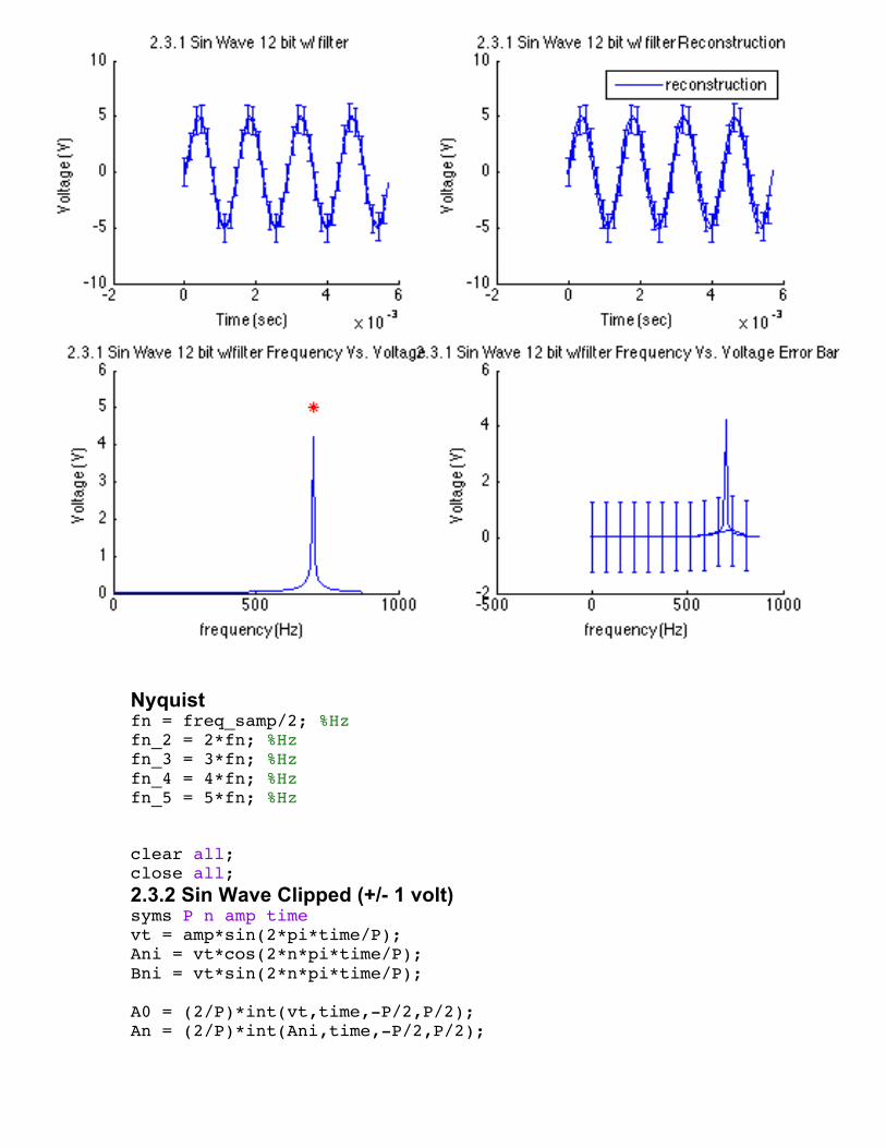
Lee120

Nyquist fn = freq_samp/2; %Hz fn_2 = 2*fn; %Hz fn_3 = 3*fn; %Hz fn_4 = 4*fn; %Hz fn_5 = 5*fn; %Hz clear all; close all; 2.3.2 Sin Wave Clipped (+/- 1 volt) syms P n amp time vt = amp*sin(2*pi*time/P); Ani = vt*cos(2*n*pi*time/P); Bni = vt*sin(2*n*pi*time/P); A0 = (2/P)*int(vt,time,-P/2,P/2); An = (2/P)*int(Ani,time,-P/2,P/2);

Lee121

Bn = (2/P)*int(Bni,time,-P/2,P/2); %Time vs. Voltage s = importdata('10_4_2016lee2.3.2_sin_clipping1dat.txt'); data = s.data; time = data(:,1); %Seconds voltage = data(:,2); %Volts amp = 5; %Volts F = 700; %Hz P = 1/F; %Hz^-1 freq_samp = 25000; %Hz i = ceil(P*freq_samp); t = time(1:4*i); %Seconds V = voltage(1:4*i); %Volts A0 = subs(A0); An = subs(An); Bn = subs(Bn); sum = 0; for n = 1:1; if n==1; B = 1; else B = Bn; end FFT = (A0/2)+(An*cos(2*n*pi*time/P)+B*sin(2*n*pi*time/P)); %Volts sum = sum + FFT; end % Uncertainty Vres = 2/(2^(16-1)); %Volts Tres = 1/(freq_samp); %Seconds Fres = freq_samp/4096; %Hz u_volt = (Vres/2)*ones(1,length(t)); %Volts u_time = .5*(1/freq_samp)*ones(1,length(t)); %Time % Frequency vs. Voltage s = importdata('10_4_2016lee2.3.2_sin_clipping2fft.txt'); data = s.data; frequency = data(:,1); %Hz vf = data(:,2); %Volts amp_freq = max(vf); %Volts f = frequency(1:144); %Hz v_f = vf(1:144); %Volts

Lee122

%Uncertainty u_v_f = (Vres/2)*ones(1,length(v_f)); %Volts u_freq = (Fres/2)*ones(1,length(f)); %Hz u_v_f1 = u_v_f(1:144); %Volts u_f1 = u_freq(1:144); %Hz Plots figure(1) subplot(3,1,1) hold on plot(t,V) title('2.3.2 Clipped Sin Wave') xlabel('Time (sec)') ylabel('Voltage (V)') errorbar(t(1:4:144),V(1:4:144),u_volt(1:4:144)) herrorbar(t(1:4:144),V(1:4:144),u_time(1:4:144)) subplot(3,1,2) hold on plot(t,sum(1:length(t))) title('2.3.2 Clipped Sin Wave Reconstruction') xlabel('Time (sec)') ylabel('Voltage (V)') legend('Reconstruction') errorbar(t(1:4:144),sum(1:4:144),u_volt(1:4:144)) herrorbar(t(1:4:144),sum(1:4:144),u_time(1:4:144)) subplot(3,1,3) hold on plot(f,v_f,700,max(voltage),'r*') title('2.1 Frequency vs. Voltage Sin Wave') xlabel('Frequency (Hz)') ylabel('Voltage (V)') errorbar(f(1:4:144),v_f(1:4:144),u_v_f1(1:4:144)) herrorbar(f(1:4:144),v_f(1:4:144),u_f1(1:4:144))

Lee123

Nyquist fn = freq_samp/2; fn_2 = 2*fn; fn_3 = 3*fn; fn_4 = 4*fn; fn_5 = 5*fn; clear all; close all; 2.3.2 Sin Wave Clipped (+/- 10 volt) syms P n amp time vt = amp*sin(2*pi*time/P); Ani = vt*cos(2*n*pi*time/P); Bni = vt*sin(2*n*pi*time/P);

Lee124

A0 = (2/P)*int(vt,time,-P/2,P/2); An = (2/P)*int(Ani,time,-P/2,P/2); Bn = (2/P)*int(Bni,time,-P/2,P/2); %Time vs. Voltage s = importdata('10_4_2016lee2.3.2_sin_clipping1dat.txt'); data = s.data; time = data(:,1); %Seconds voltage = data(:,2); %Volts amp = 5; %Volts F = 700; %Hz P = 1/F; %Hz^-1 freq_samp = 25000; %Hz i = ceil(P*freq_samp); t = time(1:4*i); %Seconds V = voltage(1:4*i); %Volts A0 = subs(A0); An = subs(An); Bn = subs(Bn); sum = 0; for n = 1:1; if n==1; B = 1; else B = Bn; end FFT = (A0/2)+(An*cos(2*n*pi*time/P)+B*sin(2*n*pi*time/P)); %Volts sum = sum + FFT; end % Uncertainty Vres = 20/(2^(16-1)); %Volts Tres = 1/(freq_samp); %Seconds Fres = freq_samp/4096; %Hz u_volt = (Vres/2)*ones(1,length(t)); %Volts u_time = .5*(1/freq_samp)*ones(1,length(t)); %Time % Frequency vs. Voltage s = importdata('10_4_2016lee2.3.2_sin_clipping2fft.txt'); data = s.data; frequency = data(:,1); %Hz vf = data(:,2); %Volts amp_freq = max(vf); %Volts f = frequency(1:144); %Hz

Lee125

v_f = vf(1:144); %Volts %Uncertainty u_v_f = (Vres/2)*ones(1,length(v_f)); %Volts u_freq = (Fres/2)*ones(1,length(f)); %Hz u_v_f1 = u_v_f(1:144); %Volts u_f1 = u_freq(1:144); %Hz Plots figure(1) subplot(3,1,1) hold on plot(t,V) title('2.3.2 Clipped Sin Wave(+/- 10)') xlabel('Time (sec)') ylabel('Voltage (V)') errorbar(t(1:4:144),V(1:4:144),u_volt(1:4:144)) herrorbar(t(1:4:144),V(1:4:144),u_time(1:4:144)) subplot(3,1,2) hold on plot(t,sum(1:length(t))) title('2.3.2 Clipped Sin Wave(+/- 10) Reconstruction') xlabel('Time (sec)') ylabel('Voltage (V)') legend('Reconstruction') errorbar(t(1:4:144),sum(1:4:144),u_volt(1:4:144)) herrorbar(t(1:4:144),sum(1:4:144),u_time(1:4:144)) subplot(3,1,3) hold on plot(f,v_f,700,max(voltage),'r*') title('2.3.2 Frequency vs. Voltage Sin Wave') xlabel('Frequency (Hz)') ylabel('Voltage (V)') errorbar(f(1:4:144),v_f(1:4:144),u_v_f1(1:4:144)) herrorbar(f(1:4:144),v_f(1:4:144),u_f1(1:4:144))

Lee126

Nyquist fn = freq_samp/2; fn_2 = 2*fn; fn_3 = 3*fn; fn_4 = 4*fn; fn_5 = 5*fn; clear all; close all; 3.1 Experimental Sin Wave syms P n amp time vt = amp*sin(2*pi*time/P); Ani = vt*cos(2*n*pi*time/P); Bni = vt*sin(2*n*pi*time/P); A0 = (2/P)*int(vt,time,-P/2,P/2); An = (2/P)*int(Ani,time,-P/2,P/2); Bn = (2/P)*int(Bni,time,-P/2,P/2);

Lee127

% Time vs. Voltage s = importdata('10_4_2016lee3.1dat.txt'); data = s.data; time = data(:,1); %Seconds voltage = data(:,2); %Volts amp = 3.85; %Volts (the function generator was not at 5 volts) F = 700; %Hz P = 1/F; %Hz^-1 freq_samp = 25000; %Hz i = ceil(P*freq_samp); t = time(1:4*i);%Seconds V = voltage(1:4*i); %Volts A0 = subs(A0); An = subs(An); Bn = subs(Bn); sum = 0; for n = 1:1; if n==1; B = amp; else B = Bn; end FFT = (A0/2)+(An*cos(2*n*pi*time/P)+B*sin(2*n*pi*time/P)); %Hz sum = sum + FFT; end % Uncertainty Vres = 20/(2^(13-1)); %Volts Tres = 1/(freq_samp); %Time Fres = freq_samp/8192; %Hz u_volt = (Vres/2)*ones(1,length(t)); %Volts u_time = .5*(1/freq_samp)*ones(1,length(t)); %Seconds % Frequency vs. Voltage s = importdata('10_4_2016lee3.1fft.txt'); data = s.data; frequency = data(:,1); %Hz vf = data(:,2); %Volts amp_freq = max(vf); %Volts f = frequency(1:144); %Hz v_f = vf(1:144); %Volts

Lee128

u_v_f = (Vres/2)*ones(1,length(v_f)); %VOlts u_freq = (Fres/2)*ones(1,length(f)); %Hz u_v_f1 = u_v_f(1:144); %Volts u_f1 = u_freq(1:144); %Hz Plots figure(1) subplot(3,1,1) hold on plot(t,V,'r') title('3.1 Experimental Sin Wave Time vs Voltage') xlabel('Time (sec)') ylabel('Voltage (V)') errorbar(t(1:4:144),V(1:4:144),u_volt(1:4:144)) herrorbar(t(1:4:144),V(1:4:144),u_time(1:4:144)) subplot(3,1,2) hold on plot(t,sum(1:length(t))) title('3.1 Experimental Sin Wave Frequency vs Voltage') xlabel('Time (sec)') ylabel('Voltage (V)') legend('Reconstruction') errorbar(t(1:4:144),sum(1:4:144),u_volt(1:4:144)) herrorbar(t(1:4:144),sum(1:4:144),u_time(1:4:144)) subplot(3,1,3) hold on plot(f,v_f,700,max(voltage),'r*') title('3.1 Sin Wave Frequency vs. Voltage') xlabel('Frequency (Hz)') ylabel('Voltage (V)') errorbar(f(1:4:144),v_f(1:4:144),u_v_f1(1:4:144)) herrorbar(f(1:4:144),v_f(1:4:144),u_f1(1:4:144))

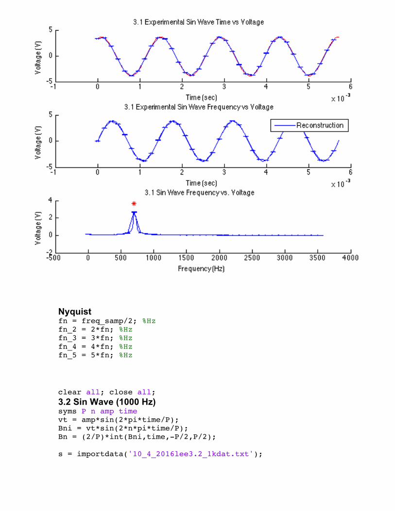
Lee129

Nyquist fn = freq_samp/2; %Hz fn_2 = 2*fn; %Hz fn_3 = 3*fn; %Hz fn_4 = 4*fn; %Hz fn_5 = 5*fn; %Hz clear all; close all; 3.2 Sin Wave (1000 Hz) syms P n amp time vt = amp*sin(2*pi*time/P); Bni = vt*sin(2*n*pi*time/P); Bn = (2/P)*int(Bni,time,-P/2,P/2); s = importdata('10_4_2016lee3.2_1kdat.txt');

Lee130

data = s.data; time = data(:,1); %Seconds voltage = data(:,2); %Volts amp = 3.85; %Volts (the function generator was not at 5 volts) F = 700; %Hz P = 1/F; %Hz^-1 freq_samp = 1000; %Hz i = ceil(P*freq_samp); t = time(1:6*i); %Seconds V = voltage(1:6*i); %Volts Bn = subs(Bn); %Volts sum = 0; A0 = 0; An = 0; for n = 1:1; if n==1; B = amp; %Volts else B = Bn; end FFT = (A0/2)+(An*cos(2*n*pi*time/P)+B*sin(2*n*pi*time/P)); %Volts sum = sum + FFT; end % Uncertainty Vres = 20/(2^(13-1)); %Volts Tres = 1/(freq_samp); %Seconds Fres = freq_samp/8192; %Hz u_volt = (Vres/2)*ones(1,length(t)); %Volts u_time = .5*(1/freq_samp)*ones(1,length(t)); %Seconds % Frequency Vs. Voltage s = importdata('10_4_2016lee3.2_1kfft.txt'); data = s.data; frequency = data(:,1); %Hz vf = data(:,2); %Volts amp_freq = max(vf); %Volts f = frequency(1:400); %Hz v_f = vf(1:400); %Volts u_v_f = (Vres/2)*ones(1,length(v_f)); %Volts u_freq = (Fres/2)*ones(1,length(f)); %Hz u_v_f1 = u_v_f(1:400); %Volts

Lee131

u_f1 = u_freq(1:400); %Hz Plots figure(1) subplot(3,1,1) hold on plot(t,V,'r') title('3.2 Sin Wave (1000Hz) Time vs. Voltage') xlabel('Time (sec)') ylabel('Voltage (V)') errorbar(t,V,u_volt) herrorbar(t,V,u_time) subplot(3,1,2) hold on plot(t,sum(1:length(t))) title('3.2 Sin Wave (1000Hz) Time vs. Voltage Reconstruction') xlabel('Time (sec)') ylabel('Voltage (V)') errorbar(t,sum(1:length(t)),u_volt) herrorbar(t,sum(1:length(t)),u_time) subplot(3,1,3) hold on plot(f,v_f) plot(290,max(v_f),'m*') title('3.2 Sin Wave (1000Hz) Frequency vs. Voltage') xlabel('Frequency (Hz)') ylabel('Voltage (V)') errorbar(f,v_f,u_v_f1) herrorbar(f,v_f,u_f1)

Lee132

Nyquist fn = freq_samp/2; %Hz fn_2 = 2*fn; %Hz fn_3 = 3*fn; %Hz fn_4 = 4*fn; %Hz fn_5 = 5*fn; %Hz clear all; close all; 3.2 Krohn-Hite on syms P n amp time vt = amp*sin(2*pi*time/P); Bni = vt*sin(2*n*pi*time/P); Bn = (2/P)*int(Bni,time,-P/2,P/2); %Time vs. Voltage

Lee133

s = importdata('10_4_2016lee3.2_krohn-hitedat.txt'); data = s.data; time = data(:,1); %Seconds voltage = data(:,2); %Volts amp = 3.85; %Volts (the function generator was not at 5 volts) F = 700; %Hz P = 1/F; %Hz^-1 freq_samp = 1000; %Hz i = ceil(P*freq_samp); t = time(1:6*i); %Seconds V = voltage(1:6*i); %Volts Bn = subs(Bn); %Volts sum = 0; A0 = 0; An = 0; for n = 1:1; if n==1; B = amp; %Volts else B = Bn; %Volts end FFT = (A0/2)+(An*cos(2*n*pi*time/P)+B*sin(2*n*pi*time/P)); sum = sum + FFT; end % Uncertainty Vres = 20/(2^(13-1)); Tres = 1/(freq_samp); Fres = freq_samp/8192; u_volt = (Vres/2)*ones(1,length(t)); u_time = .5*(1/freq_samp)*ones(1,length(t)); % Frequency vs. Voltage s = importdata('10_4_2016lee3.2_krohn-hitefft.txt'); data = s.data; frequency = data(:,1); %Hz vf = data(:,2); %Volts amp_freq = max(vf); %Volts f = frequency(1:400); %Hz v_f = vf(1:400); %Volts u_v_f = (Vres/2)*ones(1,length(v_f)); %Volts u_freq = (Fres/2)*ones(1,length(f)); %Hz

Lee134

u_v_f1 = u_v_f(1:400); %Volts u_f1 = u_freq(1:400); %Hz Plots figure(1) subplot(3,1,1) hold on plot(t,V,'r') title('3.2 Krohn-Hite Time vs. Voltage (filter on)') xlabel('Time (sec)') ylabel('Voltage (V)') errorbar(t,V,u_volt) herrorbar(t,V,u_time) subplot(3,1,2) hold on plot(t,sum(1:length(t))) title('3.2 Krohn-Hite Time vs. Voltage (filter on)') xlabel('Time (sec)') ylabel('Voltage (V)') legend('Reconstruction') errorbar(t,sum(1:length(t)),u_volt) herrorbar(t,sum(1:length(t)),u_time) subplot(3,1,3) hold on plot(f,v_f) plot(301,max(v_f),'m*') title('3.2 Krohn-Hite Frequency vs. Voltage (filter on)') xlabel('Frequency (Hz)') ylabel('Voltage (V)') errorbar(f,v_f,u_v_f1) herrorbar(f,v_f,u_f1)

Lee135

Nyquist fn = freq_samp/2; %Hz fn_2 = 2*fn; %Hz fn_3 = 3*fn; %Hz fn_4 = 4*fn; %Hz fn_5 = 5*fn; %Hz clear all; close all; 3.3 Experimental Square Wave a = importdata('10_4_2016lee3.3_squaredat.txt'); data = a.data; time = data(:,1); %Seconds voltage = data(:,2);%Volts

Lee136

amp = max(voltage); %Volts F = 700; %Hz P = 1/F; %Hz^-1 freq_samp = 25000; %Hz i = ceil(P*freq_samp); t = time(1:4*i); %Seconds V = voltage(1:4*i); %Volts %Uncertainty Vres = 20/(2^(13-1)); %VOlts Tres = 1/(freq_samp); %Seconds Fres = freq_samp/4096; %Hz u_volt = (Vres/2)*ones(1,length(t)); %Volts u_time = .5*(1/freq_samp)*ones(1,length(t)); %Seconds %Frequency vs. Voltage a = importdata('10_4_2016lee3.3_squarefft.txt'); data = a.data; frequency = data(:,1); %Hz vf = data(:,2); %Volts %Uncertainty u_v_f = (Vres/2)*ones(1,length(vf)); %Volts u_freq = (Fres/2)*ones(1,length(frequency)); %Hz Plots sum = 0; A0 = 0; An = 0; for n = [1 3 5 7 15 21]; if n==1 B = amp; else B = (amp/(pi*n))*(1-(2*cos(pi*n))+(cos(2*pi*n))); end FFT = B*sin(2*n*pi*time/P); sum = sum + FFT; end for w = 1:21 Bn(w) = (amp/(pi*w))*(1-(2*cos(pi*w))+(cos(2*pi*w))); %Volts end for e = 1:21 frq(e) = e * 700; %Hz end

Lee137

figure(1) subplot(3,1,1) hold on plot(t,V,'b') xlabel('Time (s)') ylabel('Voltage (V)') title ('3.3 Square Wave') legend('Initial') errorbar(t,V,u_volt,'k') herrorbar(t,V,u_time,'b') subplot(3,1,2) hold on plot(t,sum(1:length(t)),'r') title ('3.3 Square Wave Reconstruction') xlabel('Time (sec)') ylabel('Voltage (V)') legend('Reconstruction') errorbar(t,sum(1:length(t)),u_volt,'k') herrorbar(t,sum(1:length(t)),u_time,'r') subplot(3,1,3) hold on plot(frequency,vf,frq(1:2:end),Bn(1:2:end),'m*') xlabel('Frequency (Hz)') ylabel('Voltage (V)') title ('3.3 Square Wave Frequency vs Voltage') errorbar(frequency(1:4:144),vf(1:4:144),u_v_f(1:4:144),'k') herrorbar(frequency(1:4:144),vf(1:4:144),u_freq(1:4:144),'b')

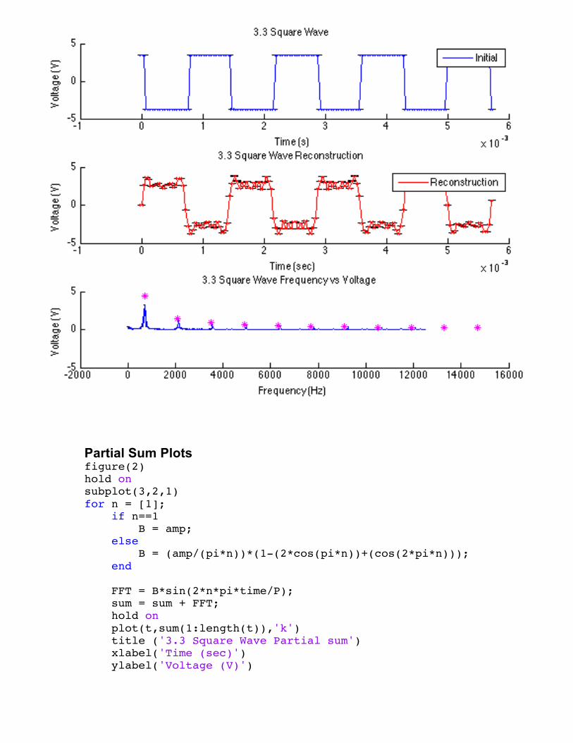
Lee138

Partial Sum Plots figure(2) hold on subplot(3,2,1) for n = [1]; if n==1 B = amp; else B = (amp/(pi*n))*(1-(2*cos(pi*n))+(cos(2*pi*n))); end FFT = B*sin(2*n*pi*time/P); sum = sum + FFT; hold on plot(t,sum(1:length(t)),'k') title ('3.3 Square Wave Partial sum') xlabel('Time (sec)') ylabel('Voltage (V)')

Lee139

errorbar(t,sum(1:length(t)),u_volt,'k') herrorbar(t,sum(1:length(t)),u_time,'b') legend ('n=1') end subplot(3,2,2) for n = [3]; if n==1 B = amp; else B = (amp/(pi*n))*(1-(2*cos(pi*n))+(cos(2*pi*n))); end FFT = B*sin(2*n*pi*time/P); sum = sum + FFT; hold on plot(t,sum(1:length(t)),'k') title ('3.3 Square Wave Partial sum') xlabel('Time (sec)') ylabel('Voltage (V)') errorbar(t,sum(1:length(t)),u_volt,'k') herrorbar(t,sum(1:length(t)),u_time,'b') legend ('n=3') end subplot(3,2,3) for n = [5]; if n==1 B = amp; else B = (amp/(pi*n))*(1-(2*cos(pi*n))+(cos(2*pi*n))); end FFT = B*sin(2*n*pi*time/P); sum = sum + FFT; hold on plot(t,sum(1:length(t)),'k') title ('3.3 Square Wave Partial sum') xlabel('Time (sec)') ylabel('Voltage (V)') errorbar(t,sum(1:length(t)),u_volt,'k') herrorbar(t,sum(1:length(t)),u_time,'b') legend ('n=5') end

Lee140

hold on subplot(3,2,4) for n = [7]; if n==1 B = amp; else B = (amp/(pi*n))*(1-(2*cos(pi*n))+(cos(2*pi*n))); end FFT = B*sin(2*n*pi*time/P); sum = sum + FFT; hold on plot(t,sum(1:length(t)),'k') title ('3.3 Square Wave Partial sum') xlabel('Time (sec)') ylabel('Voltage (V)') errorbar(t,sum(1:length(t)),u_volt,'k') herrorbar(t,sum(1:length(t)),u_time,'b') legend ('n=7') end subplot(3,2,5) hold on for n = [15]; if n==1 B = amp; else B = (amp/(pi*n))*(1-(2*cos(pi*n))+(cos(2*pi*n))); end FFT = B*sin(2*n*pi*time/P); sum = sum + FFT; hold on plot(t,sum(1:length(t)),'k') title ('3.3 Square Wave Partial sum') xlabel('Time (sec)') ylabel('Voltage (V)') errorbar(t,sum(1:length(t)),u_volt,'k') herrorbar(t,sum(1:length(t)),u_time,'b') legend ('n=15') end subplot(3,2,6) hold on

Lee141

for n = [21]; if n==1 B = amp; else B = (amp/(pi*n))*(1-(2*cos(pi*n))+(cos(2*pi*n))); end FFT = B*sin(2*n*pi*time/P); sum = sum + FFT; hold on plot(t,sum(1:length(t)),'k') title ('3.3 Square Wave Partial sum') xlabel('Time (sec)') ylabel('Voltage (V)') errorbar(t,sum(1:length(t)),u_volt,'k') herrorbar(t,sum(1:length(t)),u_time,'b') legend ('n=21') end

Lee142

Nyquist fn = freq_samp/2; %Hz fn_2 = 2*fn; %Hz fn_3 = 3*fn; %Hz fn_4 = 4*fn; %Hz fn_5 = 5*fn; %Hz clear all; close all; 3.3 Experimental Sawtooth a = importdata('10_4_2016lee3.3_sawdat.txt'); data = a.data; time = data(:,1); %Seconds voltage = data(:,2); %Volts

Lee143

amp = max(voltage); %Volts F = 700; %Hz P = 1/F; %Hz^-1 freq_samp = 25000;%Hz i = ceil(P*freq_samp); t = time(1:4*i); %Seconds V = voltage(1:4*i); %Volts % Uncertainty Vres = 20/(2^(13-1)); %Volts Tres = 1/(freq_samp); %Seconds Fres = freq_samp/4096; %Hz u_volt = (Vres/2)*ones(1,length(t)); %Volts u_time = .5*(1/freq_samp)*ones(1,length(t)); %Seconds % Frequency vs Voltage a = importdata('10_4_2016lee3.3_sawfft.txt'); data = a.data; frequency = data(:,1); %Hz vf = data(:,2); %Volts %Uncertainty u_v_f = (Vres/2)*ones(1,length(vf)); %Volts u_freq = (Fres/2)*ones(1,length(frequency)); %Hz Plots figure(1) subplot(2,2,1) hold on plot(t,V) xlabel('Time (s)') ylabel('Voltage (V)') title('3.3 Sawtooth Wave w/ filter') errorbar(t,V,u_volt) herrorbar(t,V,u_time) subplot(2,2,2) sum = 0; for n =(1:1:21); b_n = ((-2*amp)*cos(pi*n))/(pi*n); B = b_n*sin(2*pi*n*t*(1/P)); sum = sum+B; end hold on plot(t,sum) xlabel('Time (s)') ylabel('Voltage (V)') title ('3.3 Sawtooth Wave Reconstruction')

Lee144

errorbar(t,sum,u_volt,'k') herrorbar(t,sum,u_time,'b') subplot(2,2,3) hold on for w = 1:21 Bn(w) = abs(((-2*amp)*cos(pi*w))/(pi*w)); end for e = 1:21 frq(e) = e * 700; end plot(frequency,vf) plot(frq(1:1:end),Bn(1:1:end),'m*') title('3.3 Sawtooth Frequency vs. Voltage w/ filter') xlabel('Frequency (Hz)') ylabel('Voltage (V)') subplot(2,2,4) hold on errorbar(frequency(1:4:144),vf(1:4:144),u_v_f(1:4:144)) herrorbar(frequency(1:4:144),vf(1:4:144),u_freq(1:4:144)) title('3.3 Sawtooth Frequency vs. Voltage (error bar)') xlabel ('Frequency (Hz)') ylabel ('Voltage (V)')

Lee145

Partial sums figure(2) subplot(3,2,1) for n = (1:1) b_n = ((-2*amp)*cos(pi*n))/(pi*n); B = b_n*sin(2*pi*n*t*F); sum = sum+B; end hold on plot(t,sum) title ('3.3 Sawtooth Wave partial sum') xlabel('Time (s)') ylabel('Voltage (V)') errorbar(t,sum,u_volt,'k') herrorbar(t,sum,u_time,'b') legend('n = 1') sum = 0;

Lee146

subplot(3,2,2) for n = (1:3) b_n = ((-2*amp)*cos(pi*n))/(pi*n); B = b_n*sin(2*pi*n*t*(1/P)); sum = sum+B; end hold on plot(t,sum) title ('3.3 Sawtooth Wave partial sum') xlabel('Time (s)') ylabel('Voltage (V)') errorbar(t,sum,u_volt,'k') herrorbar(t,sum,u_time,'b') legend('n = 3') sum = 0; subplot(3,2,3) for n =(1:5) b_n = ((-2*amp)*cos(pi*n))/(pi*n); B = b_n*sin(2*pi*n*t*F); sum = sum+B; end hold on plot(t,sum) title('3.3 Sawtooth Wave partial sum') xlabel('Time (s)') ylabel('Voltage (V)') errorbar(t,sum,u_volt,'k') herrorbar(t,sum,u_time,'b') legend('n = 5') sum = 0; subplot(3,2,4) hold on for n = (1:7) b_n = ((-2*amp)*cos(pi*n))/(pi*n); B = b_n*sin(2*pi*n*t*F); sum = sum+B; end hold on plot(t,sum) title('3.3 Sawtooth Wave partial sum') xlabel('Time (s)')

Lee147

ylabel('Voltage (V)') errorbar(t,sum,u_volt,'k') herrorbar(t,sum,u_time,'b') legend('n = 7') sum = 0; subplot(3,2,5) for n =(1:15) b_n = ((-2*amp)*cos(pi*n))/(pi*n); B = b_n*sin(2*pi*n*t*F); sum = sum+B; end hold on plot(t,sum) title ('3.3 Sawtooth Wave partial sum') xlabel('Time (s)') ylabel('Voltage (V)') errorbar(t,sum,u_volt,'k') herrorbar(t,sum,u_time,'b') legend('n = 15') sum = 0; subplot(3,2,6) for n = (1:21) b_n = (-2*amp*cos(pi*n))/(pi*n); B = b_n*sin(2*pi*n*t*F); sum = sum+B; end hold on plot(t,sum) title ('3.3 Sawtooth Wave partial sum') xlabel('Time (s)') ylabel('Voltage (V)') errorbar(t,sum,u_volt,'k') herrorbar(t,sum,u_time,'b') legend('n = 21')

Lee148

Nyquist fn = freq_samp/2; %Hz fn_2 = 2*fn; %Hz fn_3 = 3*fn; %Hz fn_4 = 4*fn; %Hz fn_5 = 5*fn; %Hz clear all; close all; 3.3 White Noise a = importdata('10_4_2016lee3.3_whitenoisefilterdat.txt'); data = a.data; time = data(:,1); %Seconds voltage = data(:,2); %Volts amp = max(voltage); %Volts F = 700; %Hz P = 1/F; %Hz^-1

Lee149

freq_samp = 40000; %Hz i = ceil(P*freq_samp); t = time(1:4*i); %Seconds V = voltage(1:4*i); %Volts % Uncertainty Vres = 20/(2^(13-1)); %Volts Tres = 1/(freq_samp); %Seconds Fres = freq_samp/4096; %Hz u_volt = (Vres/2)*ones(1,length(t)); %Volts u_time = .5*(1/freq_samp)*ones(1,length(t)); %Seconds % Frequency vs Voltage a = importdata('10_4_2016lee3.3_whitenoisefilterfft.txt'); data = a.data; frequency = data(:,1);%Hz vf = data(:,2); %Volts %Uncertainty u_v_f = (Vres/2)*ones(1,length(vf)); %Volts u_freq = (Fres/2)*ones(1,length(frequency)); %Hz Plots figure(1) subplot(2,1,1) hold on plot(t,V) xlabel('Time (s)') ylabel('Voltage (V)') title('3.3 White Noise Time vs Voltage w/ filter') errorbar(t(1:4:232),V(1:4:232),u_volt(1:4:232)) herrorbar(t(1:4:232),V(1:4:232),u_time(1:4:232)) subplot(2,1,2) hold on plot(frequency,vf) xlabel('Frequency (Hz)') ylabel('Voltage (V)') title('3.3 White Noise Frequency vs Voltage w/ filter') errorbar(frequency(1:4:232),vf(1:4:232),u_v_f(1:4:232)) herrorbar(frequency(1:4:232),vf(1:4:232),u_freq(1:4:232))

Lee150

Lee151

Vibrations

(Table1)

Section3.1 BeamLength

(meters)Theoretical

DampedFrequency

(Hz)

SimulatedDamped

Frequency(Hz)

UncertaintyinTheoretical

DampedFrequency(Hz)

.4318 29.825 28.1585 2.1612

.4826 23.8765 22.5424 1.5485

.5588 17.8087 16.8136 1.5485

Section3.2 Damping

Coefficients (N*s/m)

TheoreticalDamped

Frequency(Hz)

SimulatedDamped

Frequency(Hz)

UncertaintyinTheoretical

DampedFrequency(Hz)

DampingRatio(zeta)

UncertaintyinDampingRatio

(zeta)

1 17.8028 16.8136 0.998 0.0258 7.3291*10^-42 17.7851 16.7576 0.998 0.0515 0.00144 17.7139 16.5895 0.998 0.1031 0.00296 17.5947 16.3092 0.998 0.1546 0.00438 17.4264 15.9169 0.9882 0.2061 0.0058

Section3.3.1 EndMass(kg) Theoretical

DampedFrequency

(Hz)

SimulatedDamped

Frequency(Hz)

UncertaintyinTheoretical

DampedFrequency(Hz)

MassEquivalenc

e(kg)

0.2 12.1366 11.3416 0.5889 0.3734 0.3 10.7789 10.0542 0.5082 0.4734

0.55 8.7197 8.1142 0.3957 0.7234

Lee152

(Table1cont.)Section3.3.2

Materials TheoreticalDamped

Frequency(Hz)

SimulatedDamped

Frequency(Hz)

UncertaintyinTheoretical

DampedFrequency(Hz)

Springconstant(k)(N/m)

UncertaintyinSpring

Constant(k)(N/m)

Aluminum 17.3675 17.0407 0.9733 713.5056 59.9811CarbonSteel 17.8087 16.8136 0.9988 2.17*10^3 182.55

StainlessSteel 16.9225 16.0075 0.99483 1.9955*10^3 167.7732 ShakerExperiment

BeamLengths(meters)

TheoreticalFrequency

(Hz)

ExperimentalFrequency(Hz)

UncertaintyinTheoretical

Frequency(Hz)

DampingRatio(zeta)

UncertaintyinDampingRatio

(zeta).4318 27.978 28 2.1612 0.3464 0.0797.4826 21.5765 22 1.5485 0.4282 0.0483.5588 16.9285 17.5 0.998 0.3105 0.0739

Hammer

Experiment

BeamLengths(meters)

TheoreticalFrequency

(Hz)

ExperimentalFrequency(Hz)

UncertaintyinTheoretical

Frequency(Hz)

DampingRatio(zeta)

UncertaintyinDampingRatio

(zeta).4318 27.978 26 1.1519 0.3464 0.3605.4826 22.4843 21 0.8222 0.3365 0.4623.5588 16.9285 16 0.5249 0.3105 0.681

Lee153

Lee154

Lee155

Lee156

Lee157

Lee158

Lee159

Lee160

Lee161

Lee162

Lee163

Lee164

Lee165

clear all; close all; 3.1 Experimental Validation Uncertainty freq_samp =50000; %Hz u_density = .005; %kg/m^3 u_youngs = .005; %N/m^2 u_length = .5*(1/32); %meters u_width = .00001*.5; %meters u_thickness= 0.00001*.5; %meters u_amplitude=.5*(10/(2^24 - 1)); %V u_freq=freq_samp/6000; %Hz u_time=1/freq_samp; %sec u_damp = .005; %N*sec/m syms L17 L19 L22 w t zeta E rho C = .01; %N*sec/m I = (1/12)*w*(t^3); %m^4 k1 = 3.*E.*I./L17.^3; %N/m V1 = L17 .*w .*t; %m^3 mass_17 = rho.* V1; %kg mass_eq17 = 33/140 .* rho .*V1; %kg Wn1 = sqrt(k1./mass_eq17); %rad/s fn1 = Wn1/(2*pi); %Hz zeta1 = C/(2*mass_17*Wn1); Wd1 = Wn1.*sqrt(1-zeta1^2); %rad/s Fd1 = Wd1/(2*pi); %Hz fn_u1 = sqrt((diff(fn1,L17).*u_length).^2+(diff(fn1,t).*u_thickness).^2 + (diff(fn1,w).*u_width).^2 + (diff(fn1,E).*u_youngs.*E).^2 + (diff(fn1,rho).*u_density.*rho).^2); %Hz Fd_u1 = sqrt((diff(Fd1,L17).*u_length).^2+(diff(Fd1,t).*u_thickness).^2 + (diff(Fd1,w).*u_width).^2 + (diff(Fd1,E).*u_youngs.*E).^2 + (diff(Fd1,rho).*u_density.*rho).^2); %Hz k2 = 3.*E.*I./L19.^3; %N/m V2 = L19 .*w .*t; %m^3 mass_19 = rho.* V2; %kg mass_eq19 = 33/140 .* rho .*V2; %kg Wn2 = sqrt(k2./mass_eq19); %rad/s fn2 = Wn2/(2*pi); %Hz zeta2 = C/(2*mass_19*Wn2); Wd2 = Wn2.*sqrt(1-zeta2^2); %rad/s Fd2 = Wd2/(2*pi); %Hz fn_u2 = sqrt((diff(fn2,L19).*u_length).^2+(diff(fn2,t).*u_thickness

Lee166

).^2 + (diff(fn2,w).*u_width).^2 + (diff(fn2,E).*u_youngs.*E).^2 + (diff(fn2,rho).*u_density.*rho).^2); Fd_u2 = sqrt((diff(Fd2,L19).*u_length).^2+(diff(Fd2,t).*u_thickness).^2 + (diff(Fd2,w).*u_width).^2 + (diff(Fd2,E).*u_youngs.*E).^2 + (diff(Fd2,rho).*u_density.*rho).^2); k3 = 3.*E.*I./L22.^3; %N/m V3 = L22 .*w .*t; %m^3 mass_22 = rho.* V3; %kg mass_eq22 = 33/140 .* rho .*V3; %kg Wn3 = sqrt(k3./mass_eq22); %rad/s fn3 = Wn3/(2*pi); %Hz zeta3 = C/(2*mass_22*Wn3); Wd3 = Wn3.*sqrt(1-zeta3^2); %rad/s Fd3 = Wd3/(2*pi); %Hz fn_u3 = sqrt((diff(fn3,L22).*u_length).^2+(diff(fn3,t).*u_thickness).^2 + (diff(fn3,w).*u_width).^2 + (diff(fn3,E).*u_youngs.*E).^2 + (diff(fn3,rho).*u_density.*rho).^2); %Hz Fd_u3 = sqrt((diff(Fd3,L22).*u_length).^2+(diff(Fd3,t).*u_thickness).^2 + (diff(Fd3,w).*u_width).^2 + (diff(Fd3,E).*u_youngs.*E).^2 + (diff(Fd3,rho).*u_density.*rho).^2); %Hz Theoretical Calculations for each length w = (0.025527 + 0.0256159 )/2; %meters t = (0.0065532 + 0.0065659)/2; %meters C = .01; E = 210*10^9; %N/m^2 rho = 7850; %Kg/m^3 I = w*(t^3)/12; %m^4 %17 Inch Beam L17 = 0.4318; %meters k17 = (3*E*I)/(L17^3); %N/m mass_17 = rho*(w*t)*L17; %kg mass_eq17 = (33*mass_17)/140; %kg Wn_17 = sqrt(k17/mass_eq17); %rad/s freq_ud_17 = Wn_17/(2*pi); %Undamped Natural Frequency zeta_17 = C/(2*mass_17*Wn_17); %Damping Coefficient ratio Wd_17 = Wn_17*sqrt(1-zeta_17^2); %rad/s freq_d_17=Wd_17/(2*pi); %Damped Natural Frequency fn_u17 = double(subs(fn_u1)); %Hz Fd_u17 = double(subs(Fd_u1)); %Hz

Lee167

%19 Inch Beam L19 = 0.4826; %meters k19 = (3*E*I)/(L19^3); %N/m mass_19 = rho*(w*t)*L19; %kg mass_eq19 = (33*mass_19)/140; %kg Wn_19 = sqrt(k19/mass_eq19); %rad/s freq_ud_19 = Wn_19/(2*pi); %Hz zeta_19 = C/(2*mass_19*Wn_19); Wd_19 = Wn_19*sqrt(1-zeta_19^2); %rad/s freq_d_19=Wd_19/(2*pi); %Hz fn_u19 = double(subs(fn_u2)); %Hz Fd_u19 = double(subs(Fd_u2)); %Hz %22 Inch Beam L22 = 0.5588; %meters k22 = (3*E*I)/(L22^3); %N/m mass_22 = rho*(w*t)*L22; %kg mass_eq22 = (33*mass_22)/140; %kg Wn_22 = sqrt(k22/mass_eq22); %rad/s freq_ud_22 = Wn_22/(2*pi); %Hz zeta_22 = C/(2*mass_22*Wn_22); Wd_22 = Wn_22*sqrt(1-zeta_22^2); %rad/s freq_d_22=Wd_22/(2*pi); %Hz fn_u22 = double(subs(fn_u3)); %Hz Fd_u22 = double(subs(Fd_u3)); %Hz Importing Data a1 = importdata('10_18_2016meyers3.1_17indat.txt'); data = a1.data; frequency17 = data(:,1); %Hz phase_angle17 = data(:,2); %rad a2 = importdata('10_18_2016meyers3.1_19indat.txt'); data = a2.data; frequency19 = data(:,1); %Hz phase_angle19 = data(:,2); %rad a3 = importdata('10_18_2016meyers3.1_22indat.txt'); data = a3.data; frequency22 = data(:,1); %Hz phase_angle22 = data(:,2); %rad a4 = importdata('10_18_2016meyers3.1_17infft.txt'); data = a4.data; freq17 = data(:,1); %Hz amp17 = data(:,2); %Volts a5 = importdata('10_18_2016meyers3.1_19infft.txt');

Lee168

data = a5.data; freq19 = data(:,1); %Hz amp19 = data(:,2); %Volts a6 = importdata('10_18_2016meyers3.1_22infft.txt'); data = a6.data; freq22 = data(:,1); %Hz amp22 = data(:,2); %Volts simulated calculations volt17 = max(amp17); %volts f_17 = freq17(find(amp17==volt17)); %Hz volt19 = max(amp19); %volts f_19 = freq19(find(amp19==volt19)); %Hz volt22 = max(amp22); %volts f_22 = freq22(find(amp22==volt22)); %Hz 3.1 Phase Angle vs. Frequency Plot & Amplitude vs. Frequency Plot figure(1); subplot(2,1,1) hold on plot(frequency17,phase_angle17,'b'); plot(frequency19,phase_angle19,'r'); plot(frequency22,phase_angle22,'g'); title ('Phase Angle vs. Frequency'); xlabel ('Frequency (Hz)'); ylabel ('Phase Angle (rad)'); legend ('17 inches','19 inches','22 inches'); subplot(2,1,2) hold on plot(freq17,amp17,'b'); plot(freq19,amp19,'r'); plot(freq22,amp22,'g'); title ('Amplitude vs. Frequency'); xlabel ('Frequency (Hz)'); ylabel ('Amplitude (V)'); legend ('17 inches','19 inches','22 inches');

Lee169

clear all; close all; 3.2 The Effects of Damping syms c1 c2 c4 c6 c8 ; syms l w t E rho ; freq_samp =50000; %Hz u_density = .005; %kg/m^3 u_youngs = .005; %N/m^2 u_length = .5*(1/32); %meters u_width = .00001*.5; %meters u_thickness= 0.00001*.5; %meters u_amplitude=.5*(10/(2^24 - 1)); %V u_freq=freq_samp/6000; %Hz u_time=1/freq_samp; %sec

Lee170

u_damp = .005; %N*sec/m v = w * t * l; %m^3 mass = rho.* v; %kg mass_eq = 33/140 .* rho .*v; %kg I = (1/12)*w*(t^3); %meters^4 k = (3*E*I)/(l^3); %N/M Wn = sqrt(k/mass_eq); %Rad/s freq_ud = Wn/(2*pi); %Undamped Natural Frequency (Hz) zeta1 = c1/(2*mass_eq*Wn); Wd1 = Wn*sqrt(1-zeta1^2); %Rad/s freq_d1 = Wd1/(2*pi); %(Hz) zeta2 = c2/(2*mass_eq*Wn); Wd2 = Wn*sqrt(1-zeta2^2); %Rad/s freq_d2 = Wd2/(2*pi); %(Hz) zeta4 = c4/(2*mass_eq*Wn); Wd4 = Wn*sqrt(1-zeta4^2); %Rad/s freq_d4 = Wd4/(2*pi); %(Hz) zeta6 = c6/(2*mass_eq*Wn); Wd6 = Wn*sqrt(1-zeta6^2); %Rad/s freq_d6 = Wd6/(2*pi); %(Hz) zeta8 = c8/(2*mass_eq*Wn); Wd8 = Wn*sqrt(1-zeta8^2); %Rad/s freq_d8 = Wd8/(2*pi); %(Hz) u_f_ud = sqrt((diff(freq_ud,l).*u_length).^2+(diff(freq_ud,t).*u_thickness).^2 + (diff(freq_ud,w).*u_width).^2 + (diff(freq_ud,E).*u_youngs.*E).^2 + (diff(freq_ud,rho).*u_density.*rho).^2); %Hz u_f_d1 = sqrt((diff(freq_d1,l).*u_length).^2+(diff(freq_d1,t).*u_thickness).^2 + (diff(freq_d1,w).*u_width).^2 + (diff(freq_d1,E).*u_youngs.*E).^2 + (diff(freq_d1,rho).*u_density.*rho).^2 + (diff(freq_d1,c1)*u_damp).^2); %Hz u_f_d2 = sqrt((diff(freq_d2,l).*u_length).^2+(diff(freq_d2,t).*u_thickness).^2 + (diff(freq_d2,w).*u_width).^2 + (diff(freq_d2,E).*u_youngs.*E).^2 + (diff(freq_d2,rho).*u_density.*rho).^2 + (diff(freq_d2,c2)*u_damp).^2); %Hz u_f_d4 =

Lee171

sqrt((diff(freq_d4,l).*u_length).^2+(diff(freq_d4,t).*u_thickness).^2 + (diff(freq_d4,w).*u_width).^2 + (diff(freq_d4,E).*u_youngs.*E).^2 + (diff(freq_d4,rho).*u_density.*rho).^2 + (diff(freq_d4,c4)*u_damp).^2); %Hz u_f_d6 = sqrt((diff(freq_d6,l).*u_length).^2+(diff(freq_d6,t).*u_thickness).^2 + (diff(freq_d6,w).*u_width).^2 + (diff(freq_d6,E).*u_youngs.*E).^2 + (diff(freq_d6,rho).*u_density.*rho).^2 + (diff(freq_d6,c6)*u_damp).^2); %Hz u_f_d8 = sqrt((diff(freq_d8,l).*u_length).^2+(diff(freq_d8,t).*u_thickness).^2 + (diff(freq_d2,w).*u_width).^2 + (diff(freq_d8,E).*u_youngs.*E).^2 + (diff(freq_d8,rho).*u_density.*rho).^2 + (diff(freq_d8,c8)*u_damp).^2); %Hz u_z1 = sqrt((diff(zeta1,w).*u_width).^2 + (diff(zeta1,t).*u_thickness).^2 + (diff(zeta1,l).*u_length).^2 + (diff(zeta1,c1).*u_damp).^2); u_z2 = sqrt((diff(zeta2,w).*u_width).^2 + (diff(zeta2,t).*u_thickness).^2 + (diff(zeta2,l).*u_length).^2 + (diff(zeta2,c2).*u_damp).^2); u_z4 = sqrt((diff(zeta4,w).*u_width).^2 + (diff(zeta4,t).*u_thickness).^2 + (diff(zeta4,l).*u_length).^2 + (diff(zeta4,c4).*u_damp).^2); u_z6 = sqrt((diff(zeta6,w).*u_width).^2 + (diff(zeta6,t).*u_thickness).^2 + (diff(zeta6,l).*u_length).^2 + (diff(zeta6,c6).*u_damp).^2); u_z8 = sqrt((diff(zeta8,w).*u_width).^2 + (diff(zeta8,t).*u_thickness).^2 + (diff(zeta8,l).*u_length).^2 + (diff(zeta8,c8).*u_damp).^2); Freq vs Phase Angle w = (0.025527 + 0.0256159 )/2; %meters t = (0.0065532 + 0.0065659)/2; %meters I = (1/12)*w*(t^3); %meters^4 rho = 7850; %Kg/m^3 E = 210*10^9; %N/m^2 l = 0.5588; %meters u_f_ud= double(subs(u_f_ud)); %Hz

Lee172

%C = 1 %N*sec/m a1 = importdata('10_18_2016meyers3.2_damping1dat.txt'); data = a1.data; frequency1 = data(:,1); %Hz phase_angle1 = data(:,2); %rad c1 = 1; %N*sec/m zeta1 = double(subs(zeta1)); Wd1 = double(subs(Wd1)); %Rad/s freq_d1 = double(subs(freq_d1)); %Hz u_f_d1 = double(subs(u_f_d1)); %Hz u_z1 = double(subs(u_z1)); %C = 2 a2 = importdata('10_18_2016meyers3.2_damping2dat.txt'); data = a2.data; frequency2 = data(:,1); %Hz phase_angle2 = data(:,2); %rad c2 = 2; %N*sec/m zeta2 = double(subs(zeta2)); Wd2 = double(subs(Wd2)); %Rad/s freq_d2 = double(subs(freq_d2)); %Hz u_f_d2 = double(subs(u_f_d2)); %Hz u_z2 = double(subs(u_z2)); %C = 4 a3 = importdata('10_18_2016meyers3.2_damping4dat.txt'); data = a3.data; frequency4 = data(:,1); %Hz phase_angle4 = data(:,2); %rad c4 = 4; %N*sec/m zeta4 = double(subs(zeta4)); Wd4 = double(subs(Wd4)); %Rad/s freq_d4 = double(subs(freq_d4)); %hz u_f_d4 = double(subs(u_f_d4)); %hz u_z4 = double(subs(u_z4)); %c = 6 a4 = importdata('10_18_2016meyers3.2_damping6dat.txt'); data = a4.data; frequency6 = data(:,1); %Hz phase_angle6 = data(:,2); %rad

Lee173

c6 = 6; %N*sec/m zeta6 = double(subs(zeta6)); Wd6 = double(subs(Wd6)); %rad/s freq_d6 = double(subs(freq_d6)); %Hz u_f_d6 = double(subs(u_f_d6)); %Hz u_z6 = double(subs(u_z6)); %c = 8 a5 = importdata('10_18_2016meyers3.2_damping8dat.txt'); data = a5.data; frequency8 = data(:,1); %Hz phase_angle8 = data(:,2); %Volts c8 = 8; %N*sec/m zeta8 = double(subs(zeta8)); Wd8 = double(subs(Wd8)); %Rad/s freq_d8 = double(subs(freq_d8)); %Hz u_f_d8 = double(subs(u_f_d8)); %Hz u_z8 = double(subs(u_z8)); Freq vs Amplitude a6 = importdata('10_18_2016meyers3.2_damping1fft.txt'); data = a6.data; freq1 = data(:,1); %Hz amp1 = data(:,2); %Volts a7 = importdata('10_18_2016meyers3.2_damping2fft.txt'); data = a7.data; freq2 = data(:,1); %Hz amp2 = data(:,2); %Volts a8 = importdata('10_18_2016meyers3.2_damping4fft.txt'); data = a8.data; freq4 = data(:,1); %Hz amp4 = data(:,2); %Volts a9 = importdata('10_18_2016meyers3.2_damping6fft.txt'); data = a9.data; freq6 = data(:,1); %Hz amp6 = data(:,2); %Volts a10 = importdata('10_18_2016meyers3.2_damping8fft.txt'); data = a10.data; freq8 = data(:,1); %Hz amp8 = data(:,2); %Volts %3.2 Phase Angle vs. Frequency Plot & Amplitude vs.

Lee174

Frequency Plot %w/Damping figure(1); subplot(2,1,1) hold on plot(frequency1,phase_angle1,'k'); plot(frequency2,phase_angle2,'g'); plot(frequency4,phase_angle4,'r'); plot(frequency6,phase_angle6,'m'); plot(frequency8,phase_angle8,'b'); title ('Phase Angle vs. Frequency w/ Damping (N*sec/m)'); xlabel ('Frequency (Hz)'); ylabel ('Phase Angle (rad)'); legend ('1','2','4','6','8'); subplot(2,1,2) hold on plot(freq1,amp1,'k'); plot(freq2,amp2,'g'); plot(freq4,amp4,'r'); plot(freq6,amp6,'m'); plot(freq8,amp8,'b'); title ('Amplitude vs. Frequency w/ Damping (N*sec/m)'); xlabel ('Frequency (Hz)'); ylabel ('Amplitude (V)'); legend ('1','2','4','6','8'); %Simulated Values volt1 = max(amp1); %volts f_1 = freq1(find(amp1==volt1)); %Hz phase1 = phase_angle1(find(freq1==f_1)); %degrees volt2 = max(amp2); %volts f_2 = freq2(find(amp2==volt2)); %hz phase2 = phase_angle2(find(freq2==f_2)); %degrees volt4 = max(amp4); %volts f_4 = freq4(find(amp4==volt4)); %hz phase4 = phase_angle4(find(freq4==f_4)); %degrees volt6 = max(amp6); %volts f_6 = freq6(find(amp6==volt6)); %hz phase6 = phase_angle6(find(freq6==f_6)); %degrees volt8 = max(amp8); %volts f_8 = freq8(find(amp8==volt8)); %hz phase8 = phase_angle8(find(freq8==f_8)); %degrees

Lee175

clear all; close all; 3.3.1 Effect of End Mass syms w t l m1 m2 m3 E rho freq_samp =50000; %Hz u_density = .005; %kg/m^3 u_youngs = .005; %N/m^2 u_length = .5*(1/32); %meters u_width = .00001*.5; %meters u_thickness= 0.00001*.5; %meters u_amplitude=.5*(10/(2^24 - 1)); %V u_freq=freq_samp/6000; %Hz u_time=1/freq_samp; %sec

Lee176

u_damp = .005; %N*sec/m I = (1/12)*w*(t^3); %meters^4 v = w * t * l; %meters^3 k = (3*E*I)/(l^3); %N/M mass = rho * v; %kg m_eq1 = (33/140*mass) + m1; %kg m_eq2 = (33/140*mass) + m2; %kg m_eq3 = (33/140*mass) + m3; %kg Wn1 = sqrt(k/m_eq1); %rad/s Wn2 = sqrt(k/m_eq2); %rad/s Wn3 = sqrt(k/m_eq3); %rad/s freq1 = Wn1/(2*pi); %Hz freq2 = Wn2/(2*pi); %Hz freq3 = Wn3/(2*pi); %Hz u_f1 = sqrt((diff(freq1,l).*u_length).^2+(diff(freq1,t).*u_thickness).^2 + (diff(freq1,w).*u_width).^2 + (diff(freq1,E).*u_youngs.*E).^2 + (diff(freq1,rho).*u_density.*rho).^2); %Hz u_f2 = sqrt((diff(freq2,l).*u_length).^2+(diff(freq2,t).*u_thickness).^2 + (diff(freq2,w).*u_width).^2 + (diff(freq2,E).*u_youngs.*E).^2 + (diff(freq2,rho).*u_density.*rho).^2); %Hz u_f3 = sqrt((diff(freq3,l).*u_length).^2+(diff(freq3,t).*u_thickness).^2 + (diff(freq3,w).*u_width).^2 + (diff(freq3,E).*u_youngs.*E).^2 + (diff(freq3,rho).*u_density.*rho).^2); %Hz l = .5588; %meters w = (0.025527 + 0.0256159 )/2; %meters t = (0.0065532 + 0.0065659)/2; %meters E = 210*10^9; %N/m^2 v = subs(v); %meters^3 I = subs(I); %Meters^4 rho = 7850; %Kg/m^3 mass = subs(mass); %kg %.2kg a1 = importdata('10_18_2016meyers3.3.1_.2kgdat.txt'); data = a1.data; frequency2kg = data(:,1); %Hz phase_angle2kg = data(:,2); %rad

Lee177

a4 = importdata('10_18_2016meyers3.3.1_.2kgfft.txt'); data = a4.data; freq2kg = data(:,1); %Hz amp2kg = data(:,2); %Volts m1 = .2; %kg m_eq1 = double(subs(m_eq1)); %kg Wn1 = double(subs(Wn1)); %rad/s freq1 = double(subs(freq1)); %Hz u_f1 = double(subs(u_f1)); %Hz volt2kg = max(amp2kg); %volts f_2 = freq2kg(find(amp2kg==volt2kg)); %Hz phase2kg = phase_angle2kg(find(frequency2kg ==f_2)); %degrees %.3kg a2 = importdata('10_18_2016meyers3.3.1_.3kgdat.txt'); data = a2.data; frequency3kg = data(:,1); %Hz phase_angle3kg = data(:,2); %rad a5 = importdata('10_18_2016meyers3.3.1_.3kgfft.txt'); data = a5.data; freq3kg = data(:,1); %Hz amp3kg = data(:,2); %Volts m2 = .3; %kg m_eq2 = double(subs(m_eq2)); %kg Wn2 = double(subs(Wn2)); %rad/s freq2 = double(subs(freq2)); %hz u_f2 = double(subs(u_f2)); %Hz volt3kg = max(amp3kg); %volts f_3 = freq3kg(find(amp3kg==volt3kg)); %Hz phase3kg = phase_angle3kg(find(frequency3kg ==f_3)); %degrees %.55kg a3 = importdata('10_18_2016meyers3.3.1_.55kgdat.txt'); data = a3.data; frequency55kg = data(:,1); %Hz phase_angle55kg = data(:,2); %rad a6 = importdata('10_18_2016meyers3.3.1_.55kgfft.txt'); data = a6.data; freq55kg = data(:,1); %Hz amp55kg = data(:,2); %Volts

Lee178

m3 = .55; %kg m_eq3 = double(subs(m_eq3)); %kg Wn3 = double(subs(Wn3)); %rad/s freq3 = double(subs(freq3)); %hz u_f3 = double(subs(u_f3)); %hz volt55kg = max(amp55kg); %volts f_55 = freq55kg(find(amp55kg==volt55kg)); %Hz phase55kg = phase_angle55kg(find(frequency55kg ==f_55)); %degrees %3.3.1 Phase Angle vs. Frequency Plot & Amplitude vs. Frequency Plot figure(1); subplot(2,1,1) hold on plot(frequency2kg,phase_angle2kg,'b'); plot(frequency3kg,phase_angle3kg,'g'); plot(frequency55kg,phase_angle55kg,'r'); title ('Phase Angle vs. Frequency w/ different masses'); xlabel ('Frequency (Hz)'); ylabel ('Phase Angle (rad)'); legend ('.2kg','.3kg','.55kg'); subplot(2,1,2) hold on plot(freq2kg,amp2kg,'b'); plot(freq3kg,amp3kg,'g'); plot(freq55kg,amp55kg,'r'); title ('Amplitude vs. Frequency w/ different masses'); xlabel ('Frequency (Hz)'); ylabel ('Amplitude (V)'); legend ('.2kg','.3kg','.55kg');

Lee179

clear all; close all; 3.3.2 Effect of Materials syms l w t c E_al E_cs E_ss rho_al rho_cs rho_ss ; freq_samp =50000; %Hz u_density = .005; %kg/m^3 u_youngs = .005; %N/m^2 u_length = .5*(1/32); %meters u_width = .00001*.5; %meters u_thickness= 0.00001*.5; %meters u_amplitude=.5*(10/(2^24 - 1)); %V u_freq=freq_samp/6000; %Hz u_time=1/freq_samp; %sec

Lee180

u_damp = .005; %N*sec/m I = (1/12)*w*t^3; %m^4 v = w * t * l; %m^3 k_al = (3*E_al*I)/(l^3); %N/m k_cs = (3*E_cs*I)/(l^3); %N/m k_ss = (3*E_ss*I)/(l^3); %N/m m_al = rho_al * v; %kg m_cs = rho_cs * v; %kg m_ss = rho_ss * v; %kg meq_al = (33/140) * m_al; %kg meq_cs = (33/140) * m_cs; %kg meq_ss = (33/140) * m_ss; %kg Wn_al = sqrt(k_al/meq_al); %rad/s Wn_cs = sqrt(k_cs/meq_cs); %rad/s Wn_ss = sqrt(k_ss/meq_ss); %rad/s Freq_al = Wn_al /(2*pi); %hz Freq_cs = Wn_cs /(2*pi); %hz Freq_ss = Wn_ss /(2*pi); %hz u_f_al = sqrt((diff(Freq_al,l).*u_length).^2+(diff(Freq_al,t).*u_thickness).^2 + (diff(Freq_al,w).*u_width).^2 + (diff(Freq_al,E_al).*u_youngs.*E_al).^2 + (diff(Freq_al,rho_al).*u_density.*rho_al).^2 + (diff(Freq_al,c)*u_damp).^2); %hz u_f_cs = sqrt((diff(Freq_cs,l).*u_length).^2+(diff(Freq_cs,t).*u_thickness).^2 + (diff(Freq_cs,w).*u_width).^2 + (diff(Freq_cs,E_cs).*u_youngs.*E_cs).^2 + (diff(Freq_cs,rho_cs).*u_density.*rho_cs).^2 + (diff(Freq_cs,c)*u_damp).^2); %hz u_f_ss = sqrt((diff(Freq_ss,l).*u_length).^2+(diff(Freq_ss,t).*u_thickness).^2 + (diff(Freq_ss,w).*u_width).^2 + (diff(Freq_ss,E_ss).*u_youngs.*E_ss).^2 + (diff(Freq_ss,rho_ss).*u_density.*rho_ss).^2 + (diff(Freq_ss,c)*u_damp).^2); %hz u_k_al = sqrt((diff(k_al,w).*u_width).^2 + (diff(k_al,t).*u_thickness).^2 + (diff(k_al,l).*u_length).^2 + (diff(k_al,E_al).*u_youngs.*E_al).^2); %N*sec/m u_k_cs = sqrt((diff(k_cs,w).*u_width).^2 + (diff(k_cs,t).*u_thickness).^2 + (diff(k_cs,l).*u_length).^2 + (diff(k_cs,E_cs).*u_youngs.*E_cs).^2); %N*sec/m

Lee181

u_k_ss = sqrt((diff(k_ss,w).*u_width).^2 + (diff(k_ss,t).*u_thickness).^2 + (diff(k_ss,l).*u_length).^2 + (diff(k_ss,E_ss).*u_youngs.*E_ss).^2); %N*sec/m w = (0.025527 + 0.0256159 )/2; %meters t = (0.0065532 + 0.0065659)/2; %meters l = .5588; %m C = .01; %N*sec/m I = subs(I); %m^4 E_al = 69*10^9; %N/m^2 E_cs = 210*10^9; %N/m^2 E_ss = 193*10^9; %N/m^2 rho_al = 2712; %kg/m^3 rho_cs = 7850; %kg/m^3 rho_ss = 7990; %kg/m^3 k_al = double(subs(k_al)); %N*sec/m k_cs = double(subs(k_cs)); %N*sec/m k_ss = double(subs(k_ss)); %N*sec/m %Aluminum a1 = importdata('10_18_2016meyers3.3.2_aluminumdat.txt'); data = a1.data; frequency_al = data(:,1); %Hz phase_angle_al = data(:,2); %rad a4 = importdata('10_18_2016meyers3.3.2_aluminumfft.txt'); data = a4.data; freq_al = data(:,1); %Hz amp_al = data(:,2); %Volts Freq_al = double(subs(Freq_al)); %hz u_f_al = double(subs(u_f_al)); %hz u_k_al = double(subs(u_k_al)); %N*sec/m %Carbon Steel a2 = importdata('10_18_2016meyers3.3.2_carbonsteeldat.txt'); data = a2.data; frequency_cs = data(:,1); %Hz phase_angle_cs = data(:,2); %rad a5 = importdata('10_18_2016meyers3.3.2_carbonsteelfft.txt'); data = a5.data; freq_cs = data(:,1); %Hz amp_cs = data(:,2); %Volts Freq_cs = double(subs(Freq_cs)); %hz u_f_cs = double(subs(u_f_cs)); %hz

Lee182

u_k_cs = double(subs(u_k_cs)); %N*sec/m %Stainless Steel a3 = importdata('10_18_2016meyers3.3.2_stainlesssteeldat.txt'); data = a3.data; frequency_ss = data(:,1); %Hz phase_angle_ss = data(:,2); %rad a6 = importdata('10_18_2016meyers3.3.2_stainlesssteelfft.txt'); data = a6.data; freq_ss = data(:,1); %Hz amp_ss = data(:,2); %Volts Freq_ss = double(subs(Freq_ss)); %hz u_f_ss = double(subs(u_f_ss)); %hz u_k_ss = double(subs(u_k_ss)); %N*sec/m %3.3.2 Plots of Frequency vs Phase Angle & Amplitude vs. Frequency figure(1); subplot(2,1,1) hold on plot(frequency_al,phase_angle_al,'b'); plot(frequency_cs,phase_angle_cs,'r'); plot(frequency_ss,phase_angle_ss,'g'); title ('Phase Angle vs. Frequency for different Materials'); xlabel ('Frequency (Hz)'); ylabel ('Phase Angle (rad)'); legend ('Aluminum','Carbon Steel','Stainless Steel'); subplot(2,1,2) hold on plot(freq_al,amp_al,'b'); plot(freq_cs,amp_cs,'r'); plot(freq_ss,amp_ss,'g'); title ('Amplitude vs. Frequency for different materials'); xlabel ('Frequency (Hz)'); ylabel ('Amplitude (V)'); legend ('Aluminum','Carbon Steel','Stainless Steel');

Lee183

Simulated Calculations volt_al = max(amp_al); %volts Simulated_Natural_Frequency_al = freq_al(find(amp_al==volt_al)); %Hz volt_cs = max(amp_cs); %volts Simulated_Natural_Frequency_cs = freq_cs(find(amp_cs==volt_cs)); %Hz volt_ss = max(amp_ss); %volts Simulated_Natural_Frequency_ss = freq_ss(find(amp_ss==volt_ss)); %hz

Lee184

clear all; close all; Experiment Shaker syms L17 L19 L22 w t zeta E rho r1 r2 r3; freq_samp =1000; %Hz u_density = .005; %kg/m^3 u_youngs = .005; %N/m^2 u_length = .5*(1/32); %meters u_width = .00001*.5; %meters u_thickness= 0.00001*.5; %meters u_amplitude=.5*(10/(2^24 - 1)); %V u_freq=freq_samp/6000; %Hz u_time=1/freq_samp; %sec u_damp = .005; %N*sec/m I = (1/12)*w*(t^3); %m^4 k1 = 3.*E.*I./L17.^3; %N/m V1 = L17 .*w .*t; %m^3 mass_17 = rho.* V1; %kg mass_eq17 = 33/140 .* rho .*V1; %kg Wn1 = sqrt(k1./mass_eq17); %rad/s fn1 = Wn1/(2*pi); %hz Wr1 = r1*2*pi; %rad/s zeta1 = sqrt((-.5)*(((Wr1/Wn1)^2)-1)); Wd1 = Wn1.*sqrt(1-zeta1^2); %rad/s Fd1 = Wd1/(2*pi); %hz k2 = 3.*E.*I./L19.^3; %N/m V2 = L19 .*w .*t; %m^3 mass_19 = rho.* V2; %kg mass_eq19 = 33/140 .* rho .*V2; %kg Wn2 = sqrt(k2./mass_eq19); %rad/s fn2 = Wn2/(2*pi); %hz Wr2 = r2*2*pi; %rad/s zeta2 = sqrt((-.5)*(((Wr2/Wn2)^2)-1)); Wd2 = Wn2.*sqrt(1-zeta2^2); %rad/s Fd2 = Wd2/(2*pi); %hz k3 = 3.*E.*I./L22.^3; %N/m V3 = L22 .*w .*t; %m^3 mass_22 = rho.* V3; %kg mass_eq22 = 33/140 .* rho .*V3; %kg Wn3 = sqrt(k3./mass_eq22); %rad/s

Lee185

fn3 = Wn3/(2*pi); %hz Wr3 = r3*2*pi; %rad/s zeta3 = sqrt((-.5)*(((Wr3/Wn3)^2)-1)); Wd3 = Wn3.*sqrt(1-zeta3^2); %rad/s Fd3 = Wd3/(2*pi); %hz u_fn1 = sqrt((diff(fn1,L17).*u_length).^2+(diff(fn1,t).*u_thickness).^2 + (diff(fn1,w).*u_width).^2 + (diff(fn1,E).*u_youngs.*E).^2 + (diff(fn1,rho).*u_density.*rho).^2); %hz u_fn2 = sqrt((diff(fn2,L19).*u_length).^2+(diff(fn2,t).*u_thickness).^2 + (diff(fn2,w).*u_width).^2 + (diff(fn2,E).*u_youngs.*E).^2 + (diff(fn2,rho).*u_density.*rho).^2); %hz u_fn3 = sqrt((diff(fn3,L22).*u_length).^2+(diff(fn3,t).*u_thickness).^2 + (diff(fn3,w).*u_width).^2 + (diff(fn3,E).*u_youngs.*E).^2 + (diff(fn3,rho).*u_density.*rho).^2); %hz u_fd1 = sqrt((diff(Fd1,L17).*u_length).^2+(diff(Fd1,t).*u_thickness).^2 + (diff(Fd1,w).*u_width).^2 + (diff(Fd1,E).*u_youngs.*E).^2 + (diff(Fd1,rho).*u_density.*rho).^2); %hz u_fd2 = sqrt((diff(Fd2,L19).*u_length).^2+(diff(Fd2,t).*u_thickness).^2 + (diff(Fd2,w).*u_width).^2 + (diff(Fd2,E).*u_youngs.*E).^2 + (diff(Fd2,rho).*u_density.*rho).^2); %hz u_fd3 = sqrt((diff(Fd3,L22).*u_length).^2+(diff(Fd3,t).*u_thickness).^2 + (diff(Fd3,w).*u_width).^2 + (diff(Fd3,E).*u_youngs.*E).^2 + (diff(Fd3,rho).*u_density.*rho).^2); %hz u_z1= sqrt((diff(zeta1,w).*u_width).^2 + (diff(zeta1,t).*u_thickness).^2 + (diff(zeta1,L17).*u_length).^2 + (diff(zeta1,r1).*u_freq).^2); u_z2 = sqrt((diff(zeta2,w).*u_width).^2 + (diff(zeta2,t).*u_thickness).^2 + (diff(zeta2,L19).*u_length).^2 + (diff(zeta2,r2).*u_freq).^2); u_z3 = sqrt((diff(zeta3,w).*u_width).^2 +

Lee186

(diff(zeta3,t).*u_thickness).^2 + (diff(zeta3,L22).*u_length).^2 + (diff(zeta3,r3).*u_freq).^2); w = (0.025527 + 0.0256159 )/2; %meters t = (0.0065532 + 0.0065659)/2; %meters C = .01; %N*sec/m I = subs(I); %m^4 rho = 7850; %kg/m^3 E = 210*10^9; %N/m^2 %17 in a = importdata('17in_shakertest.txt'); frequency17 = a(:,2); %Hz input_amplitude17 = a(:,3); %Volts output_amplitude17 = a(:,4); %Volts L17 = 0.4318; %m k1 = double(subs(k1)); %N/m r1 = 26; %hz mass_17 = double(subs(mass_17)); %kg mass_eq17 = (subs(mass_eq17)); %kg Wn1 = double(subs(Wn1)); %rad/s Wr1 = double(subs(Wr1)); %rad/s zeta1 = double(subs(zeta1)); %Damping Coefficient ratio Wd1 = double(subs(Wd1)); %rad/s fn1=double(subs(fn1)); %hz u_fn1 = double(subs(u_fn1)); %hz Fd1 = double(subs(Fd1)); %hz u_z1 = double(subs(u_z1)); freq17 = max(frequency17); %hz %19 in b = importdata('19in_shakertest.txt'); frequency19 = b(:,2); %Hz input_amplitude19 = b(:,3); %Volts output_amplitude19 = b(:,4); %Volts L19 = 0.4826; %m k2 = double(subs(k2)); %N/m r2 = 19; %hz mass_19 = double(subs(mass_19)); %kg mass_eq19 = double(subs(mass_eq19)); %kg Wn2 = double(subs(Wn2)); %rad/s zeta2 = double(subs(zeta2)); %Damping Coefficient ratio

Lee187

Wd2 = double(subs(Wd2)); %rad/s fn2 = double(subs(fn2)); %Hz u_fn2 = double(subs(u_fn2)); %hz Fd2 = double(subs(Fd2)); %hz u_z2 = double(subs(u_z2)); freq19 = max(frequency19); %hz %22 in c = importdata('22in_shakertest.txt'); frequency22 = c(:,2); %Hz input_amplitude22 = c(:,3); %Volts output_amplitude22 = c(:,4); %Volts L22 = 0.5588; %m k3 = double(subs(k3)); %N/m r3 = 16; %hz mass_22 = double(subs(mass_22)); %kg mass_eq22 = double(subs(mass_eq22)); %kg Wn3 = double(subs(Wn3)); %rad/s zeta3 = double(subs(zeta3)); %Damping Coefficient ratio Wd3 = double(subs(Wd3)); %rad/s fn3 = double(subs(fn2)); %Hz u_fn3 = double(subs(u_fn3)); %hz Fd3 = double(subs(Fd3)); %hz u_z3 = double(subs(u_z3)); freq22 = max(frequency22); %hz %Plots figure(1); subplot(3,1,1) hold on herrorbar(frequency17,output_amplitude17,ones(numel(output_amplitude17),1)*u_freq,'r'); errorbar(frequency17,output_amplitude17,ones(numel(output_amplitude17),1)*u_amplitude,'r'); plot(frequency17,output_amplitude17,'b'); title ('Amplitude vs. Frequency(17 inch)'); xlabel ('Frequency (Hz)'); ylabel ('Amplitude (V)'); legend ('herror bar','error bar'); subplot(3,1,2) hold on herrorbar(frequency19,output_amplitude19,ones(numel(output_amplitude19),1)*u_freq,'r'); errorbar(frequency19,output_amplitude19,ones(numel(output_a

Lee188

mplitude19),1)*u_amplitude,'r'); plot(frequency19,output_amplitude19,'b'); title ('Amplitude vs. Frequency (19 inch)'); xlabel ('Frequency (Hz)'); ylabel ('Amplitude (V)'); legend ('herror bar','error bar'); subplot(3,1,3) hold on herrorbar(frequency22,output_amplitude22,ones(numel(output_amplitude22),1)*u_freq,'r'); errorbar(frequency22,output_amplitude22,ones(numel(output_amplitude22),1)*u_amplitude,'r'); plot(frequency22,output_amplitude22,'b'); title ('Amplitude vs. Frequency (22 inch)'); xlabel ('Frequency (Hz)'); ylabel ('Amplitude (V)'); legend ('herror bar','error bar');

Lee189

clear all; close all; Hammer Experiment syms w t L17 L19 L22 E rho r1 r2 r3 freq_samp =50000; %Hz u_density = .005; %kg/m^3 u_youngs = .005; %N/m^2 u_length = .5*(1/32); %meters u_width = .00001*.5; %meters u_thickness= 0.00001*.5; %meters u_amplitude=.5*(10/(2^24 - 1)); %V u_freq=freq_samp/6000; %Hz u_time=1/freq_samp; %sec

Lee190

u_damp = .005; %N*sec/m I = (1/12)*w*(t^3); %m^4 k1 = 3.*E.*I./L17.^3; %N/m V1 = L17 .*w .*t; %m^3 mass_17 = rho.* V1; %kg mass_eq17 = 33/140 .* rho .*V1; %kg Wn1 = sqrt(k1./mass_eq17); %rad/s fn1 = Wn1/(2*pi); %hz Wr1 = r1*2*pi; %rad/s zeta1 = sqrt((-.5)*(((Wr1/Wn1)^2)-1)); Wd1 = Wn1.*sqrt(1-zeta1^2); %rad/s Fd1 = Wd1/(2*pi); %hz k2 = 3.*E.*I./L19.^3; %N/m V2 = L19 .*w .*t; %m^3 mass_19 = rho.* V2; %kg mass_eq19 = 33/140 .* rho .*V2; %kg Wn2 = sqrt(k2./mass_eq19); %rad/s fn2 = Wn2/(2*pi); %hz Wr2 = r2*2*pi; %rad/s zeta2 = sqrt((-.5)*(((Wr2/Wn2)^2)-1)); Wd2 = Wn2.*sqrt(1-zeta2^2); %rad/sec Fd2 = Wd2/(2*pi); %hz k3 = 3.*E.*I./L22.^3; %N/m V3 = L22 .*w .*t; %m^3 mass_22 = rho.* V3; %kg mass_eq22 = 33/140 .* rho .*V3; %kg Wn3 = sqrt(k3./mass_eq22); %rad/s fn3 = Wn3/(2*pi); %hz Wr3 = r3*2*pi; %rad/s zeta3 = sqrt((-.5)*(((Wr3/Wn3)^2)-1)); Wd3 = Wn3.*sqrt(1-zeta3^2); %rad/s Fd3 = Wd3 / (2*pi); %hz fn_u1 = sqrt((diff(fn1,L17).*u_length).^2+(diff(fn1,t).*u_thickness).^2 + (diff(fn1,w).*u_width).^2 + (diff(fn1,E).*u_youngs.*E).^2 + (diff(fn1,rho).*u_density.*rho).^2); %hz fn_u2 = sqrt((diff(fn2,L19).*u_length).^2+(diff(fn2,t).*u_thickness).^2 + (diff(fn2,w).*u_width).^2 + (diff(fn2,E).*u_youngs.*E).^2 +

Lee191

(diff(fn2,rho).*u_density.*rho).^2); %hz fn_u3 = sqrt((diff(fn3,L22).*u_length).^2+(diff(fn3,t).*u_thickness).^2 + (diff(fn3,w).*u_width).^2 + (diff(fn3,E).*u_youngs.*E).^2 + (diff(fn3,rho).*u_density.*rho).^2); %hz u_Fd1 = sqrt((diff(Fd1,L17).*u_length).^2+(diff(Fd1,t).*u_thickness).^2 + (diff(Fd1,w).*u_width).^2 + (diff(Fd1,E).*u_youngs.*E).^2 + (diff(Fd1,rho).*u_density.*rho).^2); %hz u_Fd2 = sqrt((diff(Fd2,L19).*u_length).^2+(diff(Fd2,t).*u_thickness).^2 + (diff(Fd2,w).*u_width).^2 + (diff(Fd2,E).*u_youngs.*E).^2 + (diff(Fd2,rho).*u_density.*rho).^2); %hz u_Fd3 = sqrt((diff(Fd3,L22).*u_length).^2+(diff(Fd3,t).*u_thickness).^2 + (diff(Fd3,w).*u_width).^2 + (diff(Fd3,E).*u_youngs.*E).^2 + (diff(Fd3,rho).*u_density.*rho).^2); %hz u_z1= sqrt((diff(zeta1,w).*u_width).^2 + (diff(zeta1,t).*u_thickness).^2 + (diff(zeta1,L17).*u_length).^2 + (diff(zeta1,r1).*u_freq).^2); u_z2 = sqrt((diff(zeta2,w).*u_width).^2 + (diff(zeta2,t).*u_thickness).^2 + (diff(zeta2,L19).*u_length).^2 + (diff(zeta2,r2).*u_freq).^2); u_z3 = sqrt((diff(zeta3,w).*u_width).^2 + (diff(zeta3,t).*u_thickness).^2 + (diff(zeta3,L22).*u_length).^2 + (diff(zeta3,r3).*u_freq).^2); w = (0.025527 + 0.0256159 )/2; %meters t = (0.0065532 + 0.0065659)/2; %meters I = subs(I); %m^4 rho = 7850; %kg/m^3 E = 210*10^9; %N/m^2 a = importdata('17in_hammer_testdat.txt'); data = a.data; time17 = data(:,1); %Hz output_amplitude17 = data(:,2); %Volts input_amplitude17 = data(:,3); %Volts

Lee192

b = importdata('19in_hammer_testdat.txt'); data = b.data; time19 = data(:,1); %Hz output_amplitude19 = data(:,2); %Volts input_amplitude19 = data(:,3); %Volts c = importdata('22in_hammer_testdat.txt'); data = c.data; time22 = data(:,1); %Hz output_amplitude22 = data(:,2); %Volts input_amplitude22 = data(:,3); %Volts Calculations %17 inch L17 = 0.4318; %m r1 = 26; %hz k1 = double((subs(k1))); %N/m mass_17 = double(subs(mass_17)); %kg mass_eq17 = double(subs(mass_eq17)); %kg Wn1 = double(subs(Wn1)); %rad/s zeta1 = double(subs(zeta1)); %Damping Coefficient ratio Wd1 = double(subs(Wd1)); %rad/s fn1 = double(subs(fn1)); %Hz fn_u1 = double(subs(fn_u1)); %hz Fd1 = double(subs(Fd1)); %hz u_z1= double(subs(u_z1)); u_Fd1 = double(subs(u_Fd1)); %hz a17 = max(output_amplitude17); %volts ft17 = a17/(2*pi); %hz %19 inch L19 = 0.4826; %m r2 = 21; %hz k2 = double((subs(k2))); %N/m mass_19 = double(subs(mass_19)); %kg mass_eq19 = double(subs(mass_eq19)); %kg Wn2 = double(subs(Wn2)); %rad/s zeta2 = double(subs(zeta2)); %Damping Coefficient ratio Wd2 = double(subs(Wd2)); %rad/s fn2 = double(subs(fn2)); %Hz fn_u2 = double(subs(fn_u2)); %hz Fd2 = double(subs(Fd2)); %hz u_z2= double(subs(u_z2)); u_Fd2 = double(subs(u_Fd2)); %hz a19 = max(output_amplitude19); %volts ft19 = a19/(2*pi); %hz

Lee193

%22 inch L22 = 0.5588; %m r3 = 16; %hz k3 = double((subs(k3))); %N/m mass_22 = double(subs(mass_22)); %kg mass_eq22 = double(subs(mass_eq22)); %kg Wn3 = double(subs(Wn3)); %rad/s zeta3 = double(subs(zeta3)); %Damping Coefficient ratio Wd3 = double(subs(Wd3)); %rad/s fn3 = double(subs(fn3)); %hz fn_u3 = double(subs(fn_u3)); %hz Fd3 = double(subs(Fd3)); %hz u_Fd3 = double(subs(u_Fd3)); %hz u_z3= double(subs(u_z3)); a22 = max(output_amplitude22); %volts ft22 = a22/(2*pi); %hz Amplitude vs Time Plots figure(1); subplot(3,2,1) hold on herrorbar(time17(1:100:6000),output_amplitude17(1:100:6000),(1:100:6000)*u_time,'r'); errorbar(time17(1:100:6000),output_amplitude17(1:100:6000),(1:100:6000)*u_amplitude,'r'); plot(time17,output_amplitude17,'b'); title ('Amplitude vs. Time (17 inches) (output)'); xlabel ('Time (sec)'); ylabel ('Amplitude (V)'); legend ('herror bars','error bars'); xlim([0.19 .5]) subplot(3,2,3) hold on herrorbar(time19(1:100:6000),output_amplitude19(1:100:6000),(1:100:6000)*u_time,'r'); errorbar(time19(1:100:6000),output_amplitude19(1:100:6000),(1:100:6000)*u_amplitude,'r'); plot(time19,output_amplitude19,'b'); title ('Amplitude vs. Time (19 inches) (output)'); xlabel ('Time (Sec)'); ylabel ('Amplitude (V)'); legend ('herror bar','error bar'); xlim([0.21 .5]) subplot(3,2,5) hold on

Lee194

herrorbar(time22(1:100:6000),output_amplitude22(1:100:6000),(1:100:6000)*u_time,'r'); errorbar(time22(1:100:6000),output_amplitude22(1:100:6000),(1:100:6000)*u_amplitude,'r'); plot(time22,output_amplitude22,'b'); title ('Amplitude vs. Time (22 inches) (output)'); xlabel ('Time (sec)'); ylabel ('Amplitude (V)'); legend ('herror bar','error bar'); xlim([0.39 .6]) subplot(3,2,2) hold on herrorbar(time17(1:100:6000),input_amplitude17(1:100:6000),(1:100:6000)*u_time,'r'); errorbar(time17(1:100:6000),input_amplitude17(1:100:6000),(1:100:6000)*u_amplitude,'r'); plot(time17,input_amplitude17,'b'); title ('Amplitude vs. Time (17 inches) (input)'); xlabel ('Time (sec)'); ylabel ('Amplitude (V)'); legend ('herror bar','error bar'); xlim([0.19 .25]) subplot(3,2,4) hold on herrorbar(time19(1:100:6000),input_amplitude19(1:100:6000),(1:100:6000)*u_time,'r'); errorbar(time19(1:100:6000),input_amplitude19(1:100:6000),(1:100:6000)*u_amplitude,'r'); plot(time19,input_amplitude19,'b'); title ('Amplitude vs. Time (19 inches)(input)'); xlabel ('Time (Sec)'); ylabel ('Amplitude (V)'); legend('herror bar','error bar'); xlim([0.21 .25]) subplot(3,2,6) hold on herrorbar(time22(1:100:6000),input_amplitude22(1:100:6000),(1:100:6000)*u_time,'r'); errorbar(time22(1:100:6000),input_amplitude22(1:100:6000),(1:100:6000)*u_amplitude,'r'); plot(time22,input_amplitude22,'b'); title ('Amplitude vs. Time (22 inches) (input)'); xlabel ('Time (sec)'); ylabel ('Amplitude (V)'); legend ('herror bar', 'error bar');

Lee195

xlim([0.395 .41])

Amplitude vs Frequency Hammer Experiment a2 = importdata('17in_hammer_testfft.txt'); data = a2.data; freq17 = data(:,1); %hz output_amp17 = data(:,2); %volts input_amp17 = data(:,3); %volts b2 = importdata('19in_hammer_testfft.txt'); data = b2.data; freq19 = data(:,1); %hz output_amp19 = data(:,2); %volts input_amp19 = data(:,3); %volts c2 = importdata('22in_hammer_testfft.txt');

Lee196

data = c2.data; freq22 = data(:,1); %hz output_amp22 = data(:,2); %volts input_amp22 = data(:,3); %volts v17 = max(output_amp17); %volts f17 = freq17(find(output_amp17==v17)); %hz v19 = max(output_amp19); %volts f19 = freq19(find(output_amp19==v19)); %hz v22 = max(output_amp22); %volts f22 = freq22(find(output_amp22==v22)); %hz Amplitude vs. output Frequency figure(2) subplot(3,1,1) hold on herrorbar(freq17,output_amp17,ones(numel(output_amp17),1)*u_freq,'r-'); errorbar(freq17,output_amp17,ones(numel(output_amp17),1)*u_amplitude,'r'); plot(freq17,output_amp17,'b'); title ('Amplitude vs. Frequency (17 inch) (output)'); xlabel ('Frequency (Hz)'); ylabel ('Amplitude (V)'); legend ('herror bar','error bar'); xlim([0 1400]) subplot(3,1,2) hold on herrorbar(freq19,output_amp19,ones(numel(output_amp19),1)*u_freq,'r-'); errorbar(freq19,output_amp19,ones(numel(output_amp19),1)*u_amplitude,'r'); plot(freq19,output_amp19,'b'); title ('Amplitude vs. Frequency (19 inch) (output)'); xlabel ('Frequency (Hz)'); ylabel ('Amplitude (V)'); legend ('Herror Bar','error bar'); xlim([0 1400]) subplot(3,1,3) hold on herrorbar(freq22,output_amp22,ones(numel(output_amp22),1)*u_freq,'r-'); errorbar(freq22,output_amp22,ones(numel(output_amp22),1)*u_amplitude,'r'); plot(freq22,output_amp22,'b'); title ('Amplitude vs. Frequency (output)');

Lee197

xlabel ('Frequency (Hz)'); ylabel ('Amplitude (V)'); legend ('22 inch'); xlim([0 1400])

Amplitude vs Input Frequency figure(3) subplot(3,1,1) hold on plot(freq17(1:2000),input_amp17(1:2000),'b'); title ('Amplitude vs. Frequency (input)'); xlabel ('Frequency (Hz)'); ylabel ('Amplitude (V)'); legend ('17 inch'); subplot(3,1,2)

Lee198

hold on plot(freq19(1:2000),input_amp19(1:2000),'b'); title ('Amplitude vs. Frequency (input)'); xlabel ('Frequency (Hz)'); ylabel ('Amplitude (V)'); legend ('19 inch'); subplot(3,1,3) hold on plot(freq22(1:2000),input_amp22(1:2000),'b'); title ('Amplitude vs. Frequency (input)'); xlabel ('Frequency (Hz)'); ylabel ('Amplitude (V)');

legend ('22 inch');

Lee199

Mag of Response 17 inch Beam real_17_out = real(fft(output_amplitude17)); %volts img_17_out = imag(fft(output_amplitude17)); %volts real_17_in = real(fft(input_amplitude17)); %volts img_17_in = real(fft(input_amplitude17)); %volts mag_17_out = sqrt(real_17_out.^2+img_17_out.^2); %volts mag_17_in = sqrt(real_17_in.^2+img_17_in.^2); %volts phase17_o = atan2(img_17_out,real_17_out); %volts phase17_i = atan2(img_17_in,real_17_in); %volts phase17_out = phase17_o*(180/pi); %degrees phase17_in = phase17_i*(180/pi); %degrees mr17 = mag_17_out / mag_17_in; mag_response_17 = mean(mr17); 19 inch Beam real_19_out = real(fft(output_amplitude19)); %volts img_19_out = imag(fft(output_amplitude19)); %volts real_19_in = real(fft(input_amplitude19)); %volts img_19_in = real(fft(input_amplitude19)); %volts mag_19_out = sqrt(real_19_out.^2+img_19_out.^2); %volts mag_19_in = sqrt(real_19_in.^2+img_19_in.^2); %volts phase19_o = atan2(img_19_out,real_19_out); %rad phase19_i = atan2(img_19_in,real_19_in); %rad phase19_out = phase19_o*(180/pi); %degrees phase19_in = phase19_i*(180/pi); %degrees mr19 = mag_19_out / mag_19_in; mag_response_19 = mean(mr19); 22 inch Beam real_22_out = real(fft(output_amplitude22)); %volts img_22_out = imag(fft(output_amplitude22)); %volts real_22_in = real(fft(input_amplitude22)); %volts img_22_in = real(fft(input_amplitude22)); %volts mag_22_out = sqrt(real_22_out.^2+img_22_out.^2); %volts mag_22_in = sqrt(real_22_in.^2+img_22_in.^2); %volts phase22_o = atan2(img_22_out,real_22_out); %rad phase22_i = atan2(img_22_in,real_22_in); %rad phase22_out = phase22_o*(180/pi); %degrees phase22_in = phase22_i*(180/pi); %degrees mr22 = mag_22_out / mag_22_in; mag_response_22 = mean(mr22); Plots of Magnitude of Response figure(4) subplot(3,2,1) hold on plot(freq17,mag_17_out);

Lee200

title ('Magnitude of Response vs. Frequency (output)'); xlabel ('Frequency (Hz)'); ylabel ('Magnitude of Response (V)'); legend ('17 inch'); subplot(3,2,2) hold on plot(freq17,mag_17_in); title('Magnitude of Response vs. Frequency(input)'); xlabel ('Frequency (Hz)'); ylabel ('Magnitude of Response (V)'); legend ('17 inch') subplot(3,2,3) hold on plot(freq19,mag_19_out); title('Magnitude of Response vs. Frequency (output)'); xlabel ('Frequency (Hz)'); ylabel ('Magnitude of Response (V)'); legend ('19 inch'); subplot(3,2,4) hold on plot(freq19,mag_19_in); title('Magnitude of Response vs.Frequency (input)'); xlabel ('Frequency (Hz)'); ylabel ('Magnitude of Response (V)'); legend ('19 inch'); subplot(3,2,5) hold on plot(freq22,mag_22_out); title('Magnitude of Response vs. Frequency (output)'); xlabel ('Frequency (Hz)'); ylabel ('Magnitude of Response (V)'); legend ('22 inch'); subplot(3,2,6) hold on plot(freq22,mag_22_in); title('Magnitude of Response vs. Frequency (input)'); xlabel ('Frequency (Hz)'); ylabel ('Magnitude of Response (V)'); legend ('22 inch');

Lee201

Phase Lag Plots figure(5) subplot (2,1,1) hold on plot(freq17(1:300),phase17_out(1:300)) title('Phase Lag vs. Frequency(output)'); xlabel('Frequency (Hz)'); ylabel('Phase Lag (degrees)'); legend ('17 inch'); subplot (2,1,2) hold on plot(freq17(1:300),phase17_in(1:300)) title('Phase Lag vs. Frequency (input)'); xlabel('Frequency (Hz)');

Lee202

ylabel('Phase Lag (degrees)'); legend ('17 inch'); figure(6) subplot(2,1,1) hold on plot(freq19(1:300),phase19_out(1:300)) title('Phase Lag vs. Frequency (output)'); xlabel('Frequency (Hz)'); ylabel('Phase Lag (degrees)'); legend ('19 inch'); subplot(2,1,2) hold on plot(freq19(1:300),phase19_in(1:300)) title('Phase Lag vs. Frequency (input)'); xlabel('Frequency (Hz)'); ylabel('Phase Lag (degrees)'); legend ('19 inch'); figure(7) subplot(2,1,1) hold on plot(freq22(1:300),phase22_out(1:300)) title('Phase Lag vs. Frequency (output)'); xlabel('Frequency (Hz)'); ylabel('Phase Lag (degrees)'); legend ('22 inch'); subplot(2,1,2) hold on plot(freq22(1:300),phase22_in(1:300)) title('Phase Lag vs.Frequency(input)'); xlabel('Frequency (Hz)'); ylabel('Phase Lag (degrees)'); legend ('22 inch');

Lee203

Lee204

Additional Questions clear all close all m = 100; %kg meq = (33/140)*m; %kg k = 912; %N/m Wn = sqrt(k/meq); %rad/s Fn = Wn/(2*pi); %Hz x0 = 5; %m v0 = 0; %m/s c1 = 0; %kg/s c2 = 100; %kg/s c3 = 604; %kg/s

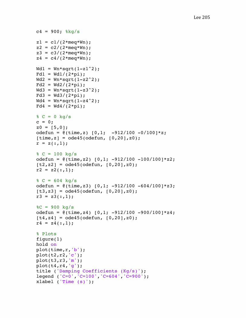
Lee205

c4 = 900; %kg/s z1 = c1/(2*meq*Wn); z2 = c2/(2*meq*Wn); z3 = c3/(2*meq*Wn); z4 = c4/(2*meq*Wn); Wd1 = Wn*sqrt(1-z1^2); Fd1 = Wd1/(2*pi); Wd2 = Wn*sqrt(1-z2^2); Fd2 = Wd2/(2*pi); Wd3 = Wn*sqrt(1-z3^2); Fd3 = Wd3/(2*pi); Wd4 = Wn*sqrt(1-z4^2); Fd4 = Wd4/(2*pi); % C = 0 kg/s c = 0; z0 = [5,0]; odefun = @(time,z) [0,1; -912/100 -0/100]*z; [time,z] = ode45(odefun, [0,20],z0); r = z(:,1); % C = 100 kg/s odefun = @(time,z2) [0,1; -912/100 -100/100]*z2; [t2,z2] = ode45(odefun, [0,20],z0); r2 = z2(:,1); % C = 604 kg/s odefun = @(time,z3) [0,1; -912/100 -604/100]*z3; [t3,z3] = ode45(odefun, [0,20],z0); r3 = z3(:,1); %C = 900 kg/s odefun = @(time,z4) [0,1; -912/100 -900/100]*z4; [t4,z4] = ode45(odefun, [0,20],z0); r4 = z4(:,1); % Plots figure(1) hold on plot(time,r,'b'); plot(t2,r2,'c'); plot(t3,r3,'m'); plot(t4,r4,'g'); title ('Damping Coefficients (Kg/s)'); legend ('C=0','C=100','C=604','C=900'); xlabel ('Time (s)');

Lee206

ylabel ('Position (m)');

Lee207

ExtraCredit:Lab2cDroneDropTests

Abstract:

Droneshaveincreasinglybecomemorepopularandmoreaffordableforconsumers.Eitherforfilmmakingorforhobby,dronescancomeinavarietyofpackages.CompanieslikeDJIhavecomeoutwithalineoftechnologicallyadvancedandaffordablequadcopterswhichpeopleuseforfilmmaking.Withdronesbecomingsopopularinsuchashorttimemeanssafetyregulationsonthesetypesofdronescouldnotbeimplementedintime.People,withoutanyformaltrainingorlicenses,areflyingtechnologythatiscapableofreachinganaltitudeof6000mandflyingatspeedsof20m/s.

Thepossibilityofthesedronesseriouslyinjuringsomeoneisshockinglyhigh.

Inexperiencecombinedwithhardwarethatisbeyondthatofasimpletoyisadeadlymixture.Inthislabweexperimentedwithadronethatisdroppedfromapredeterminedheightontomultiplefacesofthedronetosimulateadronefallingoutofthesky.Keepinmindthesetestswereconductedusingonemodelanddronescanrangeinsizeandmass.

TheFederalAviationAdministration(FAA)iscurrentlytacklingthiscrisison

howtoregulatedronesandunmannedaerialunits.Basedontestsandcalculationsconductedwearehopefulinsettingabaselineofacceptablenumberswhichdronecompanieswillhavetoincorporatewhendesigningtheirproducts.

Intro Tosimulatethedamagecausedbythedroneweusedballisticgel,tosimulatehumanflesh,andapolycarbonatesheettosimulateotherobjectslikecars,houses,windowsetc.Wedroppedthedronesusingapinloaded,ceilingmounteddroprigattachedtoacable,whichwepulled.Thedronewassuspendedatthemaximumheightthespaceallowedandtheballisticgelandpolycarbonatesheetwereplaceddirectlybelowit.Wequantizedtheamountofdamagedonebyitsimpactperformanceanditwascalculatedforeachtestwiththeequation,

𝐼𝑃 = 𝐾𝐸/𝑎𝑟𝑒𝑎 TheFAAestablishedthatdronesweightingfrom2-5lbcannotexceed12J/cm^2.Weusedcaliperstomeasurethearea,whichmadecontactwiththematerials,andthenweusedatapemeasuretocalculatetheheight.Uncertaintywascalculatedusingthezero-thorderuncertaintymethod.Tocalculatetheresponseoftheimpactweusedaslamstick.Theslamstickmeasuresg-forcesandwasstoredin

(eq.1)

Lee208

a3dprintedenclosureattachedtothedrone.Thentookthedataandbackedoutvelocityandkineticenergy.

𝑃𝐸 = 𝑚𝑔ℎ 𝐾𝐸 =12𝑚𝑣

!

Thispieceoftechnologywascrucialtocapturetheinstantaneousimpactforces;itisalsoanexampleofdigitalsignalprocessing.Theanalogforcethatthatwasconvertedtoadigitalsignal,whichweusedinourcalculations. TheaccelerometerintheSlamStickmeasuredg-forcesinallaxisandwhendroppedinoneorientationweonlyusedthatdatainthataxis.Weonlyexperimentedwiththedronefallingverticallydownandnotasifitweremovingintheairthenfalling.Ifthiswerearealscenario,thedrone’srotorbladeswouldalsobespinning.Thesebladesspinathighrpmandcouldinducemoredamageifitweretomakecontactwithhumanfleshoranyotherstructure.

Procedure Background: The FAA recently chartered the micro-unmanned aircraft

systems (µUAS) aviation rulemaking committee (ARC)1 to establish viable

performance standards and requirements for FAA certified drones. In this lab,

we will be looking at class two drones (~ 2-5 lb range). The performance criteria

that the µARC establishes for this class of drone is that the impact of the failing

drone not exceed 12 J/cm2. To capture the energy element of this criteria we will

be attaching a Slam-Stick accelerometer to the drone. Capturing the area element

is a much more complicated task. Currently, we are investigating the usefulness

of high-speed digital image correlation (DIC) to attain an accurate and

standardized area measurement. However, for the purposes of these

experiments you will be given relevant area approximations, and your task is to

determine the energy transfer during impact of a particular drop test.

1http://www.faa.gov/regulations_policies/rulemaking/committees/documents/media/MUASARC-02242016.pdf2http://info.mide.com/hubfs/datasheets/slam-stick-vibration-data-loggers-datasheet.pdf?__hssc=190384372.5.1477258583475&__hstc=190384372.026a7fdb6f31c4f8ccf79d59506baa49.1477258583474.1477258583474.1477258583474.1&hsCtaTracking=c32024f3-178f-

(eq.2,3)

Lee209

Materials:

• 3lb “Game of Drones“ Hiro Quad-Copter

• Slam-Stick X Metal2

• Pin loaded, ceiling mounted, drop rig

• 8020 Aluminum testing bed for interchangeable testing materials

• Synthetic ballistic gelatin

• Polycarbonate sheet

• Plexiglass panel

Procedure:

1. Place plexiglass panel with two gelatin blocks onto test bed such that the

weather-stripping sits on top of the metal corner brackets of the test bed.

2. Securely mount drone’s drop cradle to drop rig. Measure distance from

Slam-Stick housing to testing material.

3. Remove drone from drop rig. Turn on Slam-Stick and insert into housing

on drone. Re-secure drone to drop rig. Make note of the direction in

which the drone is falling in the Slam-Stick’s coordinate system.

4. Remove ladder and any other extraneous material from test area. Ensure

everyone is a safe distance from test area. Pull the drop pin.

5. Remove the Slam-Stick and turn it off.

6. Open Slam-Stick data. Identify primary impact event. Note max g’s

experienced during primary impact event.

7. Remove plexiglass panel with gelatin blocks. Insert polycarbonate sheet

into corner brackets of test bed.

2http://info.mide.com/hubfs/datasheets/slam-stick-vibration-data-loggers-datasheet.pdf?__hssc=190384372.5.1477258583475&__hstc=190384372.026a7fdb6f31c4f8ccf79d59506baa49.1477258583474.1477258583474.1477258583474.1&hsCtaTracking=c32024f3-178f-4f3b-bbf1-6ec4d131432f%7Cbba56a47-81d6-4103-a678-76dc75b24772

Lee210

8. Repeat steps 2-6 for new testing material.

9. How does the different material effect impact? How might a different

drop orientation effect impact?

Results

Thefirstexperimentwelookedatwasthedronefallingontotheballisticsgel

strikingwiththebottomfaceofthedrone.Theballisticsgelweusedwasconstructedentirelyfromthegel,howeverifyouweretothinkofthehumananatomy,therearebonesthatlieonlycentimetersbelowourskin.Sorealisticallywecannotassumeballisticgelcantotallyresemblehumanflesh.Theimpactperformancefortheflatballisticgelwascalculatedtobethelowestvalue,.2099

(Graph1)

Lee211

J/cm^2.ThisdidnotexceedtheFAA’svalueof12J/cm^2butweonlydroppedthedronefromaheightof2.4892meters.

Incomparisontheaccelerationwasmuchlowerintheflatpolycarbonatetest

withthedronefallingonitsface.Ingraph2wehavemultipleimpactsaftertheinitialimpact.Intesting,wehadthedronereboundoffthepolycarbonatesheetandfallontotheground.Velocitywascalculatedbyintegratingovertheaccelerationcurvethenplottingagainsttime.

Theimpactperformancefortheflatimpactonapolycarbonatesheetwascalculatedtobe.3302J/cm^2.Realisticallyadronehasasmallpercentchanceoffallingdirectlyflatontosomething,insteaditwouldtumbleandimpactatanangle.Wethensetupthedronesoitwouldimpacttheballisticsgelononeofitslegs.Theareaofthelegwas5.18cm^2wheretheareaoftheflatsurfacewas111.9cm^2,weshouldseeanincreaseinimpactperformanceduetothedecreaseinsurfaceareaoftheimpact.

(Graph2)

Lee212

(Graph3)

Ingraph3weseesimilargraphstograph2wherethedronereboundsaftertheinitialimpact.Theimpactperformancecalculatedwhendroppedontoballisticgelwithonelegwas2.377J/cm^2,whichwasthegreatestvalueoutofallthetests.Itwasnearly10timestheimpactperformanceoftheflatballisticgeltest.Theonelegontopolycarbonatetestwasalsohigherthantheflatsurfaceontopolycarbonatetest.However,afterlookingatallthetests,themostdangerouswaythedronecanimpactisononeleg.

ForcomparisontheDJIphantom4,whichisintheweightrangetheFAAset,hasamaximumaltitudeof499meters.Giventhataltitude,thepotentialenergy

Lee213

wouldbe6151Joules.Ifalltheenergywasconservedandbecamekineticenergy,theimpactperformancewouldbe55J/cm^2.Thiswouldnotbeanexpectablenumberbecauseitisnearly5times12J/cm^2.(Graph4)

Finally,welookedatthedronefallingontopolycarbonatewithoneleg.Theimpactperformancewasstillhigherthanthosewesawwhenthedronelandedflatbutitwasnothigherthanthepreviousexperimentwhenitwasdroppedontoballisticgel.

Lee214

Conclusion

Fromthelimitedexperimentswelookedatinlabwherethedroneisdroppedfromaround3mwecancomfortablysaydronesarewellintheboundaryof12J/cm^2.Ifadronefellflatwithfromaheightof108.45mitwouldhaveanimpactperformanceof12J/cm^2.Howeverifthedronedidhappentofallandimpactwithjustoneleg,itwouldonlyneedtobe4.92mifenergywasconserved.4.92metersisonly16ftoralittleover1floorofabuilding.AnythingoverwouldviolateFAArulesandpotentiallycauseseriousinjuryanddamage. Thistestwaslimitedtoafeworientationsatwhichthedronefellandwasinidealconditions.Somedroneswithinthisweightclasscanflyupto15m/s,whichis33mph.Dronecompaniesarecontinuouslyexpandingtheirlineofdronesandmakingthemmoresophisticatedandcapableofmuchmore.ThecompanyDJIjustreleasedtheirlatestmodel,theDJIInspireIIthatiscapableofreaching67mphandastaggering5000m(DJI.com).Italsodoesthisataweightof7.5lbs.(itechpost1).Althoughthisspecificmodelisprobablyoutofsomepeoplespricerangeandnottoomanyofthesewillbeflyingaround,companiesareincreasinglyimprovingtheirtechnologyandcomingoutwithdronesthatcanflyhigherandfasterthatmightleadtomoredamageiftheylosecontrol. TheFAAhastoestablishguidelinesthatencompassallunmannedaircraftsystemsandnotjustthe2-5lb.weightrangeandwaystodronesfromreachingaltitudeswhereitwillexceedtheirvalueof12J/cm^2.Eitherdronecompaniescanimplementsafetymeasuresinthedronesprogrammingwhereitdeploysaparachutewhenitfailstoslowitsdecentoryouwouldhavetolimitthedronescapabilitytoflyoveracertainspeedandcertainaltitude.

References(DJI.com)http://store.dji.com/product/inspire-2#/?_k=n58bk5(itechpost)http://www.itechpost.com/articles/55068/20161117/dji-inspire-2-quick-review-new-drone-two-cameras-lovers.htm

Lee215

Appendix(Table1)

Mass(kg)

Area(cm^2) Height(in)

Maxacceleration(m/s^2)

MaxVelocity(m/s)

ImpactPerformance(J/cm^2)

FlatClearGel 1.258 111.5445 2.4892 8.7598*10^3 2.191 0.2099FlatPolycarbonate 1.258 111.5445 2.7432 903.92 1.6224 0.3302OneLegClearGel 1.298 5.1871 2.1082 359.4829 1.3469 2.3774OneLegPolycarbonate 1.298 5.1871 2.3622 738.61 0.9713 0.4742

(Graph1)

Lee216

(Graph2)

Lee217

Lee218

(Graph3)

Lee219

(Graph4)

Lee220

%%Lab2C Drone Drop Test %Flat_ClearGel clear all; close all; syms d h area = (pi*(d^2))/4; %cm^2 u_tape = .5*(1/32)*.0254; %meters u_cal = .5*.001; %cm u_area = sqrt((diff(area,d)*u_cal).^2); %cm h = 98*.0254; %inches to meters h2 = 499.872; %meters, regulated limit v0 = 0; %m/s d = (11.914 + 11.907 + 11.931)/3; %cm m = 1.258; %kg area = double(subs(area)); %cm^2 u_area = double(subs(u_area)); %cm^2 a = importdata('Flat_ClearGel.csv'); time = a(:,1); z_accel = a(:,4); z = z_accel * 9.8 ;%G's to m/s^2 zmax = max(z); figure(1) subplot(2,1,1) hold on plot(time,z,'b'); title ('Acceleration vs. Time (Z axis)'); xlabel ('Time (sec)'); ylabel ('Acceleration (m/s^2)'); legend ('Flat Clear Gel'); xlim([93.3868 93.4]); total = 0; z_v = trapz(time,z); %z velocity m/s for i = 2:length(time)-1 total(i) = total(i-1) + (time(i+1)-time(i))*((z(i)+z(i+1))/2); end zv = total; %m/s

Lee221

figure(1) subplot(2,1,2) hold on; plot(time(1:301),zv); title ('Velocity vs. Time (Z axis)'); xlabel('Time (sec)'); ylabel('Velocity (m/s)'); legend ('Flat Clear Gel'); xlim([93.3845 93.401]); figure(2) hold on e =0; for l = (1:5:h2) e = e + (m * 9.81 * h2); plot(l,e,'.'); end title ('Potential Energy at different heights') xlabel ('Height (m)'); ylabel ('PE (J)'); pe = m*9.81*h; %Joules pe2 = m*9.81*h2; %Joules ke = .5*m*(total.^2); %Joules impact_preformance = ke/area; %J/cm^2 vmax = zv(find(z== zmax)); %Experimental vf = sqrt(2*9.81*h); %Theoretical vf2 = sqrt(2*9.81*h2); %if a drone fell from its maximum allowed height

Lee222

%Flat_polycarb clear all; close all; syms d h area = (pi*(d^2))/4; %cm^2 u_tape = .5*(1/32)*.0254; %meters u_cal = .5*.001; %cm u_area = sqrt((diff(area,d)*u_cal).^2); %cm h = 108*.0254; %inches to meters h2 = 499.872; %meters, regulated limit v0 = 0; %m/s d = (11.914 + 11.907 + 11.931)/3; %cm m = 1.258; %kg area = double(subs(area)); %cm^2

Lee223

u_area = double(subs(u_area)); %cm^2 a = importdata('Flat_Polycarb.csv'); time = a(:,1); z_accel = a(:,4); z = z_accel * 9.8 ;%G's to m/s^2 zmax = max(z); figure(1) subplot(2,1,1) hold on plot(time,z,'b'); title ('Acceleration vs. Time (Z axis)'); xlabel ('Time (sec)'); ylabel ('Acceleration (m/s^2)'); legend ('Flat Clear Gel'); xlim([53.93 54.1]); total = 0; z_v = trapz(time,z); %z velocity m/s for i = 2:length(time)-1 total(i) = total(i-1) + (time(i+1)-time(i))*((z(i)+z(i+1))/2); end zv = total; %m/s figure(1) subplot(2,1,2) hold on; plot(time(1:3185),zv); title ('Velocity vs. Time (Z axis)'); xlabel('Time (sec)'); ylabel('Velocity (m/s)'); legend ('Flat Clear Gel'); xlim([53.925 54.085]); figure(2) hold on e =0; for l = (1:5:h2) e = e + (m * 9.81 * h2); plot(l,e,'.'); end

Lee224

title ('Potential Energy at different heights') xlabel ('Height (m)'); ylabel ('PE (J)'); pe = m*9.81*h; %Joules pe2 = m*9.81*h2; %Joules ke = .5*m*(total.^2); %Joules impact_preformance = ke/area; %J/cm^2 vmax = zv(find(z== zmax)); %Experimental vf = sqrt(2*9.81*h); %Theoretical vf2 = sqrt(2*9.81*h2); %if a drone fell from its maximum allowed height

Lee225

%OneLeg_ClearGel clear all; close all; syms d t h area = d*t; %cm^2 u_tape = .5*(1/32)*.0254; %meters u_cal = .5*.001; %cm u_area = sqrt((diff(area,d)*u_cal).^2+(diff(area,t).*u_cal).^2); %cm h = 83*.0254; %inches to meters h2 = 499.872; %meters, regulated limit v0 = 0; %m/s t = 0.787; %cm d = 6.591; %cm m = 1.298; %kg area = double(subs(area)); %cm^2 u_area = double(subs(u_area)); %cm^2 a = importdata('OneLeg_ClearGel.csv'); data = a.data; time = data(:,1); y_accel = data(:,3); y = y_accel * 9.8 ;%G's to m/s^2 ymax = max(y); figure(1) subplot(2,1,1) hold on plot(time,y,'b'); title ('Acceleration vs. Time (Y axis)'); xlabel ('Time (sec)'); ylabel ('Acceleration (m/s^2)'); legend ('One Leg Clear Gel'); %xlim([53.93 54.1]); total = 0; y_v = trapz(time,y); %z velocity m/s for i = 2:length(time)-1 total(i) = total(i-1) + (time(i+1)-time(i))*((y(i)+y(i+1))/2);

Lee226

end yv = total; %m/s figure(1) subplot(2,1,2) hold on; plot(time(1:5184),yv); title ('Velocity vs. Time (Z axis)'); xlabel('Time (sec)'); ylabel('Velocity (m/s)'); legend ('One Leg Clear Gel'); %xlim([53.925 54.085]); figure(2) hold on e =0; for l = (1:5:h2) e = e + (m * 9.81 * h2); plot(l,e,'.'); end title ('Potential Energy at different heights') xlabel ('Height (m)'); ylabel ('PE (J)'); pe = m*9.81*h; %Joules pe2 = m*9.81*h2; %Joules ke = .5*m*(total.^2); %Joules impact_preformance = ke/area; %J/cm^2 vmax = yv(find(y== ymax)); %Experimental vf = sqrt(2*9.81*h); %Theoretical vf2 = sqrt(2*9.81*h2); %if a drone fell from its maximum allowed height

Lee227

%OneLeg_PolyCarb clear all; close all; syms d t h area = d*t; %cm^2 u_tape = .5*(1/32)*.0254; %meters u_cal = .5*.001; %cm u_area = sqrt((diff(area,d)*u_cal).^2+(diff(area,t).*u_cal).^2); %cm h = 93*.0254; %inches to meters h2 = 499.872; %meters, regulated limit

Lee228

v0 = 0; %m/s t = 0.787; %cm d = 6.591; %cm m = 1.298; %kg area = double(subs(area)); %cm^2 u_area = double(subs(u_area)); %cm^2 a = importdata('OneLeg_Polycarb.csv'); data = a.data; time = data(:,1); y_accel = data(:,3); y = y_accel * 9.8 ;%G's to m/s^2 ymax = max(y); figure(1) subplot(2,1,1) hold on plot(time,y,'b'); title ('Acceleration vs. Time (Y axis)'); xlabel ('Time (sec)'); ylabel ('Acceleration (m/s^2)'); legend ('One Leg Polycarb'); %xlim([53.93 54.1]); total = 0; y_v = trapz(time,y); %z velocity m/s for i = 2:length(time)-1 total(i) = total(i-1) + (time(i+1)-time(i))*((y(i)+y(i+1))/2); end yv = total; %m/s figure(1) subplot(2,1,2) hold on; plot(time(1:2690),yv); title ('Velocity vs. Time (Z axis)'); xlabel('Time (sec)'); ylabel('Velocity (m/s)'); legend ('One Leg PolyCarb'); %xlim([53.925 54.085]); figure(2)

Lee229

hold on e =0; for l = (1:5:h2) e = e + (m * 9.81 * h2); plot(l,e,'.'); end title ('Potential Energy at different heights') xlabel ('Height (m)'); ylabel ('PE (J)'); pe = m*9.81*h; %Joules pe2 = m*9.81*h2; %Joules ke = .5*m*(total.^2); %Joules impact_preformance = ke/area; %J/cm^2 vmax = yv(find(y== ymax)); %Experimental vf = sqrt(2*9.81*h); %Theoretical vf2 = sqrt(2*9.81*h2); %if a drone fell from its maximum allowed height

Lee230

Published with MATLAB® R2014a