very-near-field solutions for far-field problems
TRANSCRIPT

Very-Near-Field Solutions
for
Far-Field Problems

Local representation by Electronic Instrument Associates
Frank Krozel – (630) 924-1600
http://www.electronicinstrument.com

Agenda
Corporate Information
Introduction to Near-Field
Very-Near-Field Solution
Very-Near-Field Implementation
RFxpert Validation
RFxpert Test Applications
RFxpert Demonstration
Conclusion

Corporate Information

An Established Company
Private Canadian corporation since 1989
– Coverage in 49 countries
Unique and patented products for RF and EMI
– Very-near-field magnetic measurements
Recognized innovative products

A Leader
World Leading Developer of Visual Real-Time
EM and RF Diagnostic Solutions
Antenna and PCB Designers
Product Integration and Verification Engineers
Pre-Compliance Not Compliance

Exciting Value Proposition
Substantially Reduce Project Development Costs
Dramatically Increase Designer Productivity
Significantly Accelerate Time-to-Market
1 Hour in a Chamber or 1 Second with EMSCAN?
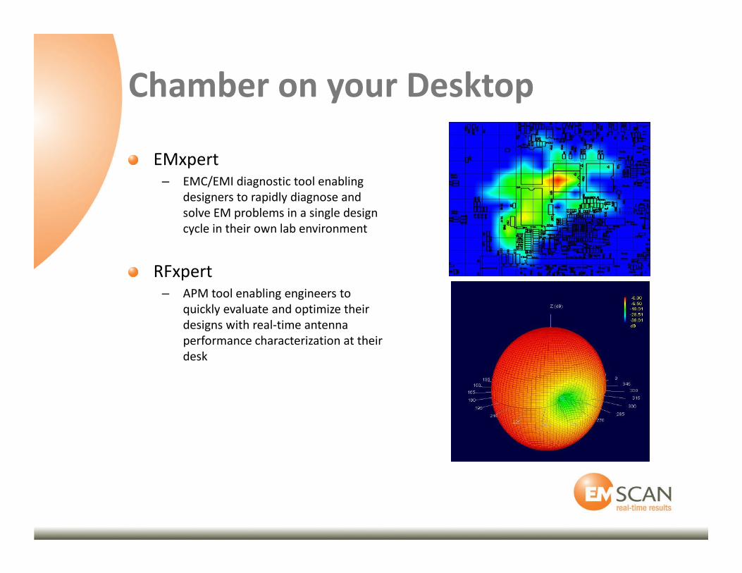
Chamber on your Desktop
EMxpert– EMC/EMI diagnostic tool enabling
designers to rapidly diagnose and
solve EM problems in a single design
cycle in their own lab environment
RFxpert– APM tool enabling engineers to
quickly evaluate and optimize their
designs with real-time antenna
performance characterization at their
desk
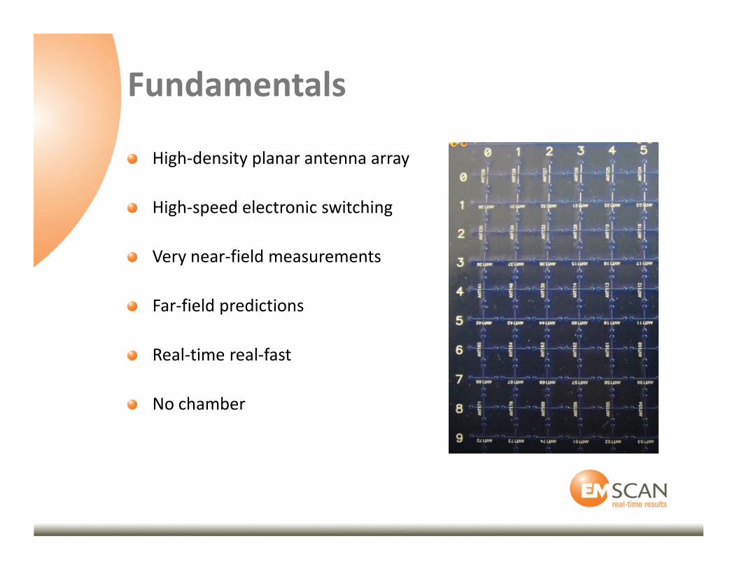
Fundamentals
High-density planar antenna array
High-speed electronic switching
Very near-field measurements
Far-field predictions
Real-time real-fast
No chamber

Introduction to Near-Field
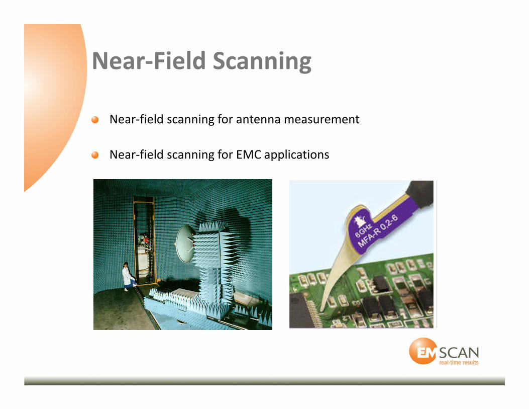
Near-Field Scanning
Near-field scanning for antenna measurement
Near-field scanning for EMC applications
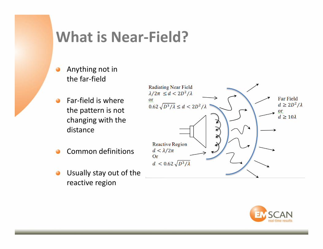
What is Near-Field?
Anything not in
the far-field
Far-field is where
the pattern is not
changing with the
distance
Common definitions
Usually stay out of the
reactive region
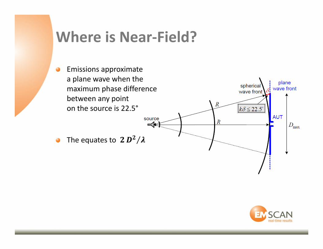
Where is Near-Field?
Emissions approximate
a plane wave when the
maximum phase difference
between any point
on the source is 22.5°
The equates to ��� �⁄
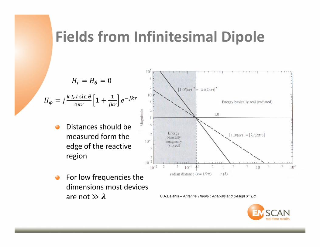
Fields from Infinitesimal Dipole
C.A.Balanis – Antenna Theory : Analysis and Design 3rd Ed.
�� � ��� ��� �
���1 �
�
������
�� � �� � 0
Distances should be
measured form the
edge of the reactive
region
For low frequencies the
dimensions most devices
are not≫ �
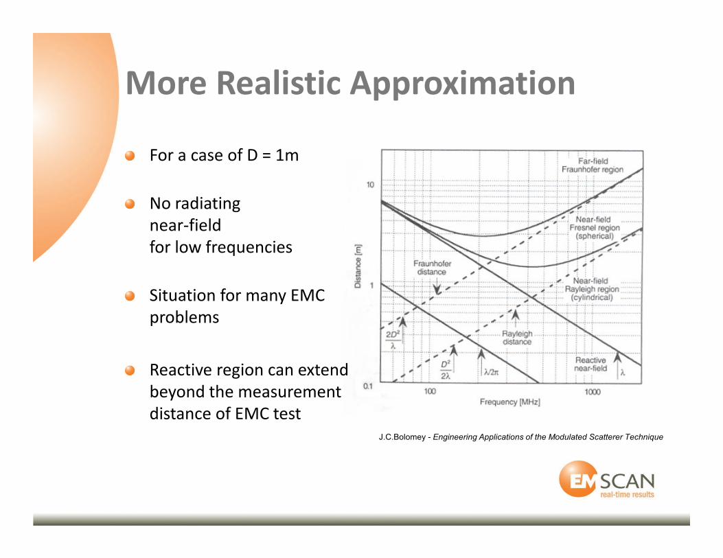
More Realistic Approximation
For a case of D = 1m
No radiating
near-field
for low frequencies
Situation for many EMC
problems
Reactive region can extend
beyond the measurement
distance of EMC test
J.C.Bolomey - Engineering Applications of the Modulated Scatterer Technique
RF Test Solution
Typically looking for far-field parameters
– Gain, efficiency, pattern are basic measures
– More complex applications such as Envelope
Correlation, Axial Ratio and Beam Forming
Debugging via near-field
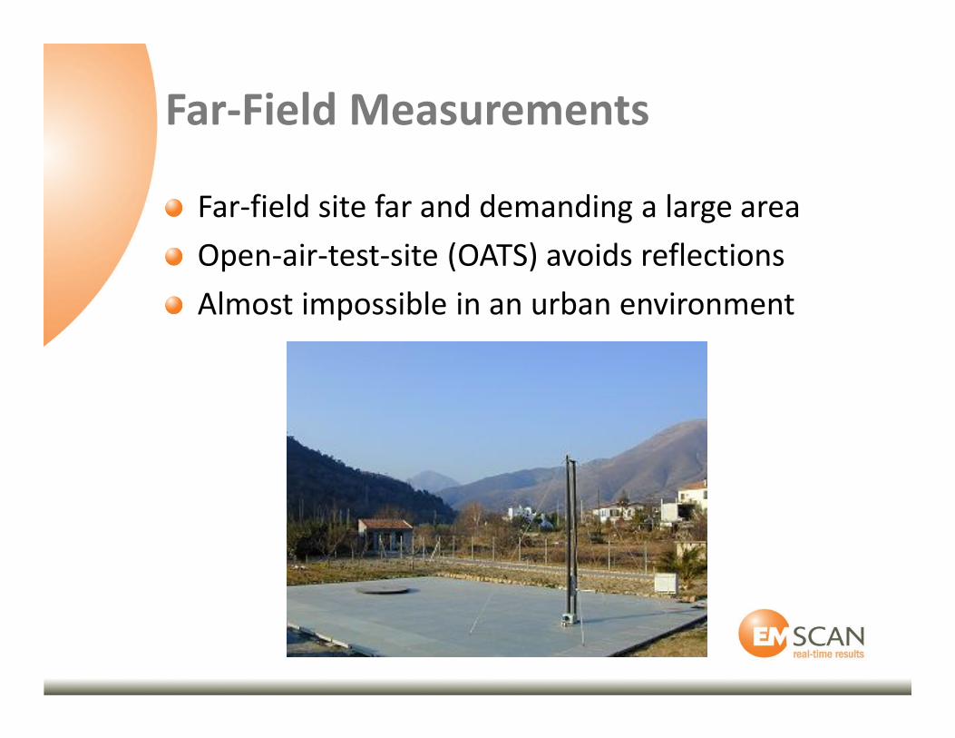
Far-Field Measurements
Far-field site far and demanding a large area
Open-air-test-site (OATS) avoids reflections
Almost impossible in an urban environment
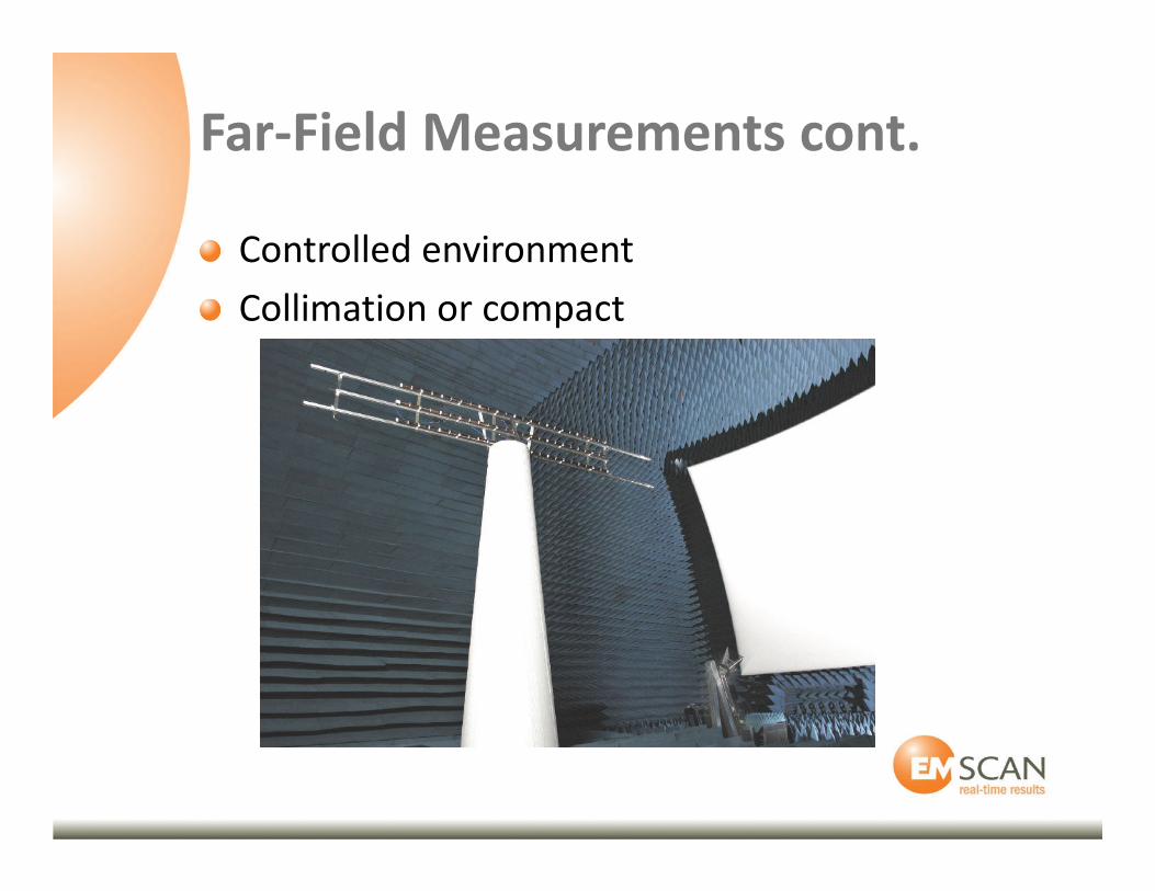
Far-Field Measurements cont.
Controlled environment
Collimation or compact
Near-Field Alternative
Various competing parameters
– Not always clear cut answer
Near-field is much smaller
– Less area
Theoretically no loss of information
Near-Field Measurements
Near-field measurement
Near to Far projections
Far to Near projections
Near to other Near projections
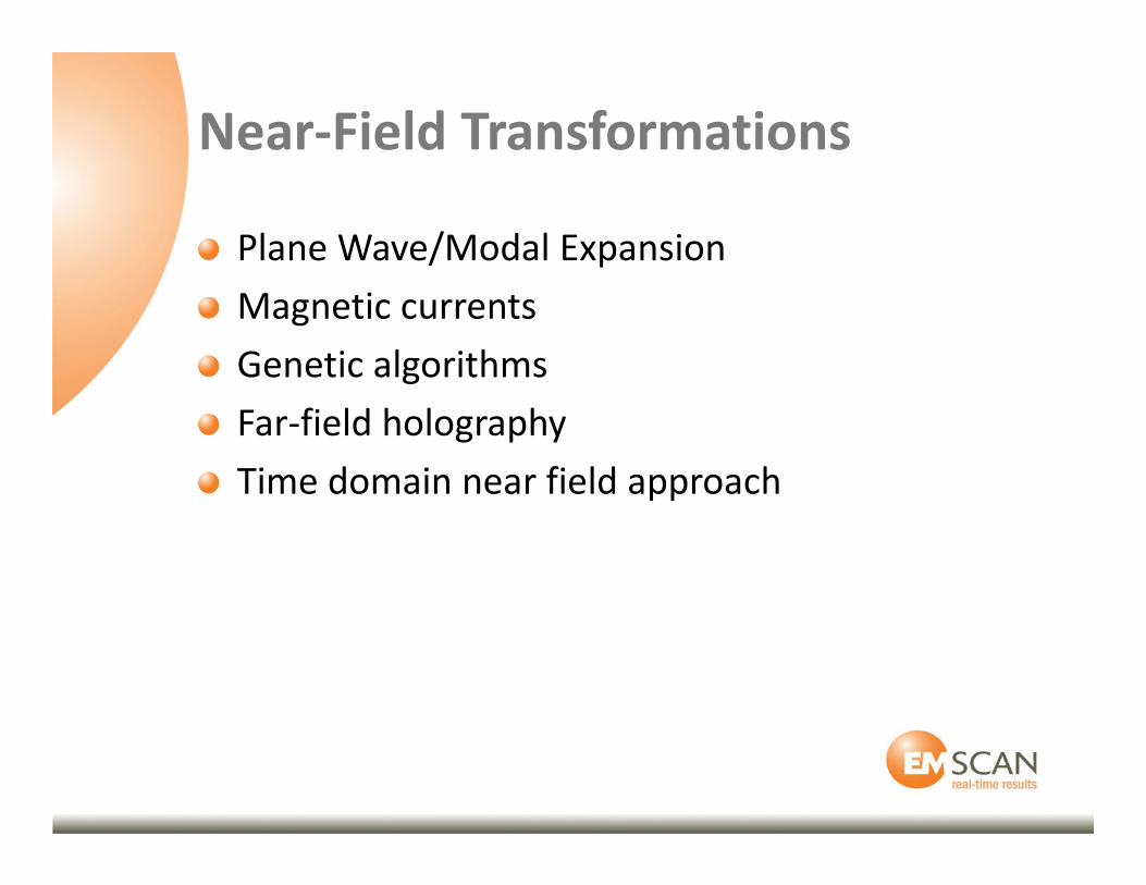
Near-Field Transformations
Plane Wave/Modal Expansion
Magnetic currents
Genetic algorithms
Far-field holography
Time domain near field approach
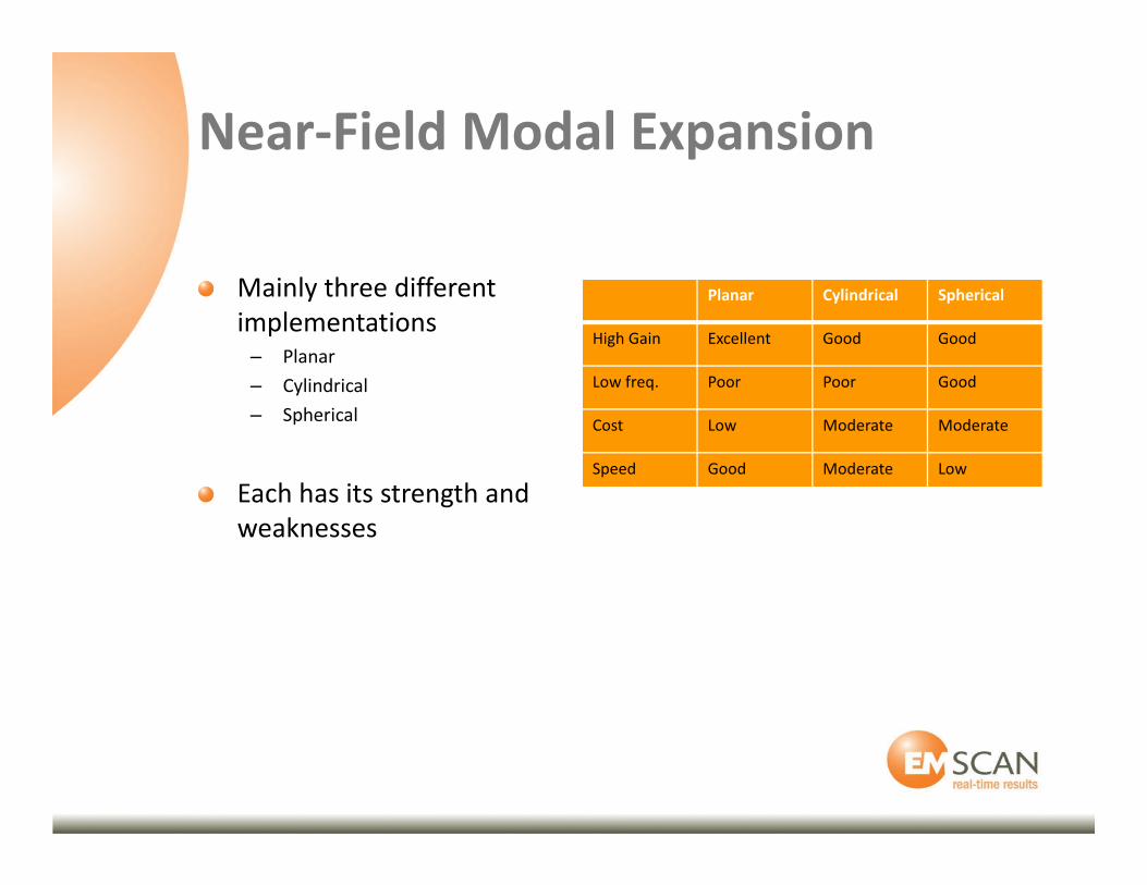
Near-Field Modal Expansion
Mainly three different
implementations– Planar
– Cylindrical
– Spherical
Each has its strength and
weaknesses
Planar Cylindrical Spherical
High Gain Excellent Good Good
Low freq. Poor Poor Good
Cost Low Moderate Moderate
Speed Good Moderate Low
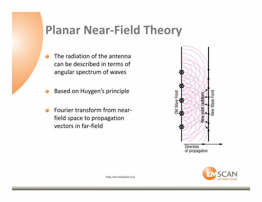
Planar Near-Field Theory
The radiation of the antenna
can be described in terms of
angular spectrum of waves
Based on Huygen’s principle
Fourier transform from near-
field space to propagation
vectors in far-field
Image: www.schoolphysics.co.uk
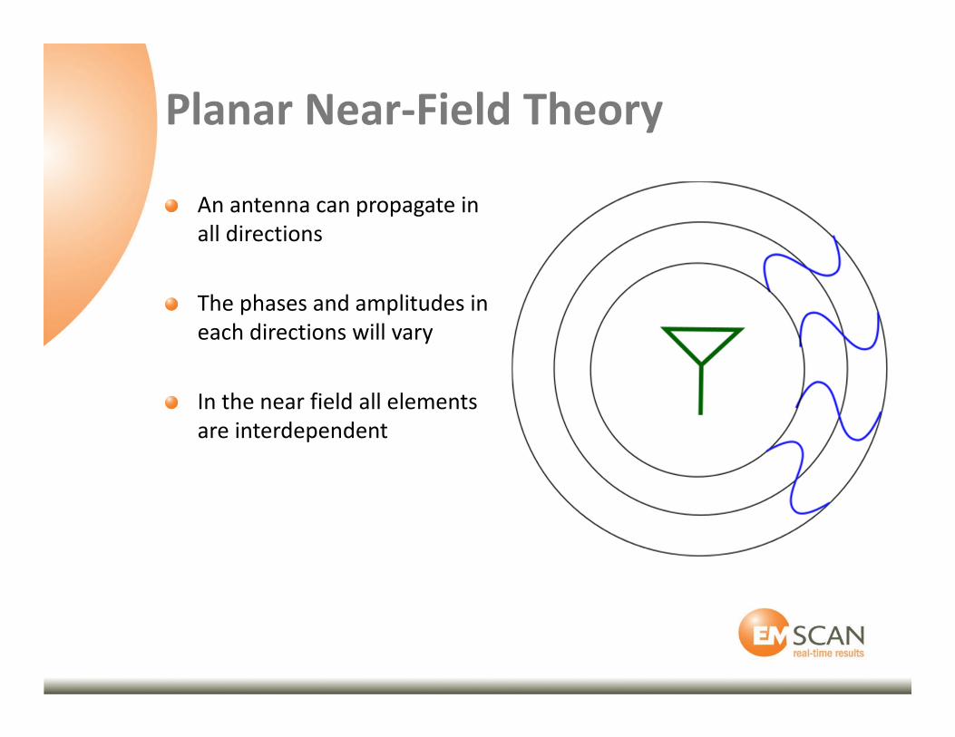
Planar Near-Field Theory
An antenna can propagate in
all directions
The phases and amplitudes in
each directions will vary
In the near field all elements
are interdependent
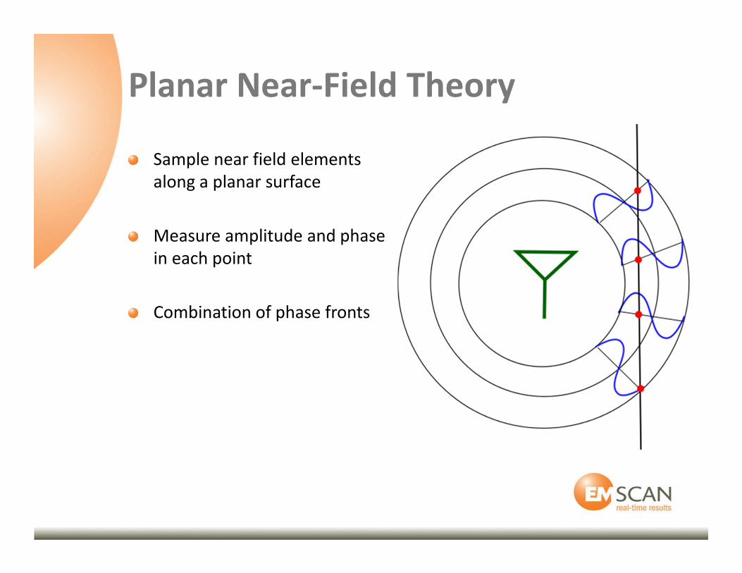
Planar Near-Field Theory
Sample near field elements
along a planar surface
Measure amplitude and phase
in each point
Combination of phase fronts
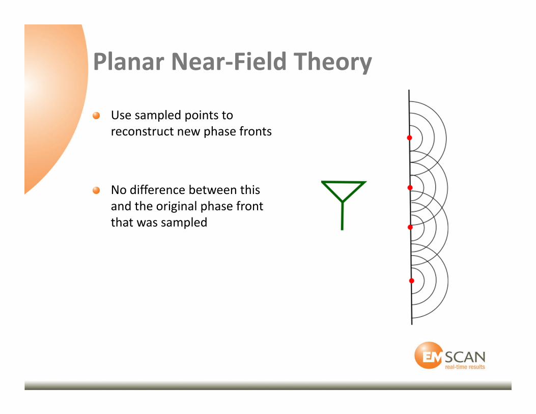
Planar Near-Field Theory
Use sampled points to
reconstruct new phase fronts
No difference between this
and the original phase front
that was sampled
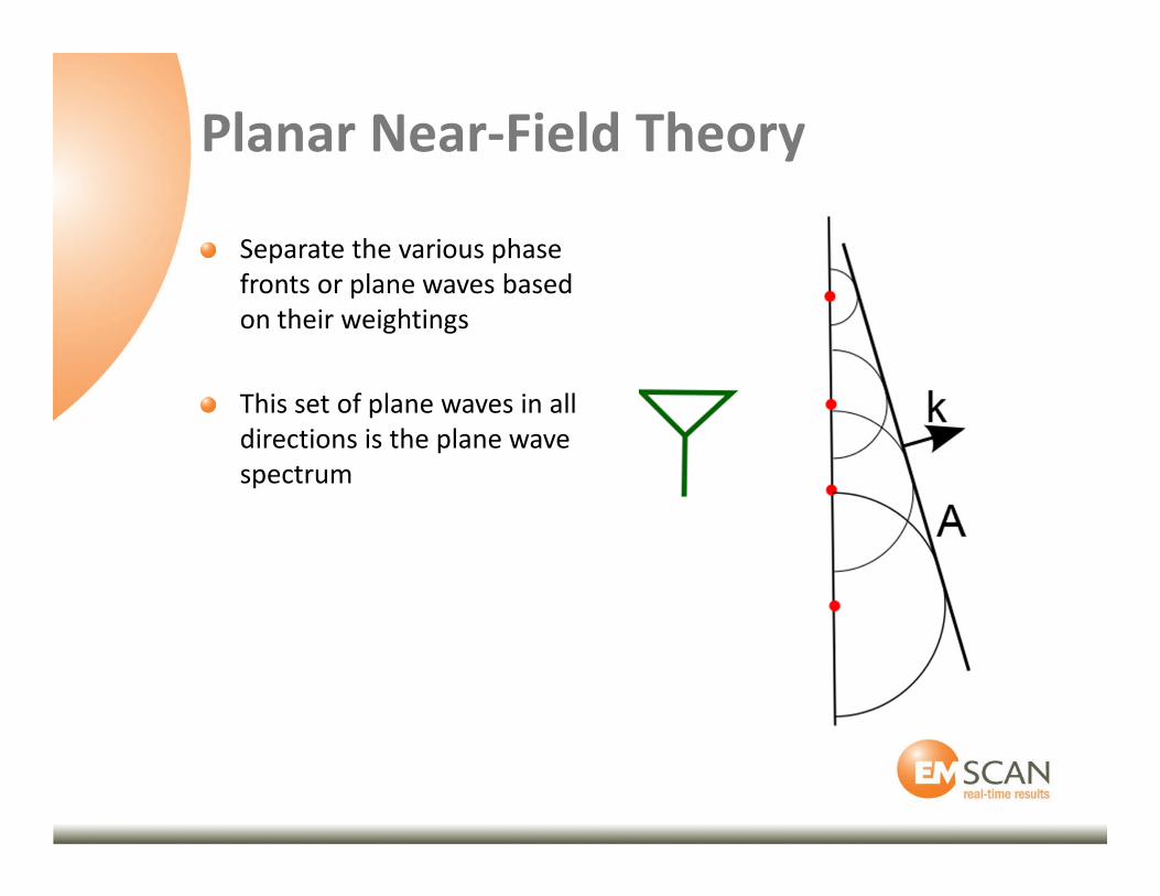
Planar Near-Field Theory
Separate the various phase
fronts or plane waves based
on their weightings
This set of plane waves in all
directions is the plane wave
spectrum
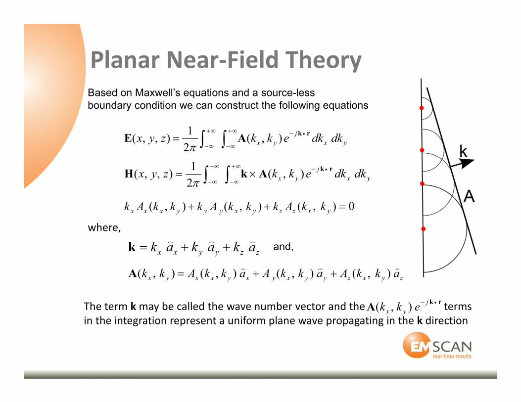
The term k may be called the wave number vector and the terms
in the integration represent a uniform plane wave propagating in the k direction
yx
j
yx dkdkekkzyxrk
AE•−∞+
∞−
∞+
∞− ∫∫= ),(2
1),,(
π
yx
j
yx dkdkekkzyxrk
AkH•−∞+
∞−
∞+
∞− ∫∫ ×= ),(2
1),,(
π
0),(),(),( =++ yxzzyxyyyxxx kkAkkkAkkkAk
Based on Maxwell’s equations and a source-less
boundary condition we can construct the following equations
zzyyxx akakak)))
++=k
where,
rk
A•− j
yx ekk ),(
zyxzyyxyxyxxyx akkAakkAakkAkk)))),(),(),(),( ++=A
and,
Planar Near-Field Theory
yx
ykxkjzkj
yxxtx dkdkeekkAzyxE yxtz)(
),(2
1),,(
+−−∞+
∞−
∞+
∞− ∫∫=π
yx
ykxkjzkj
yxyty dkdkeekkAzyxE yxtz)(
),(2
1),,(
+−−∞+
∞−
∞+
∞− ∫∫=π
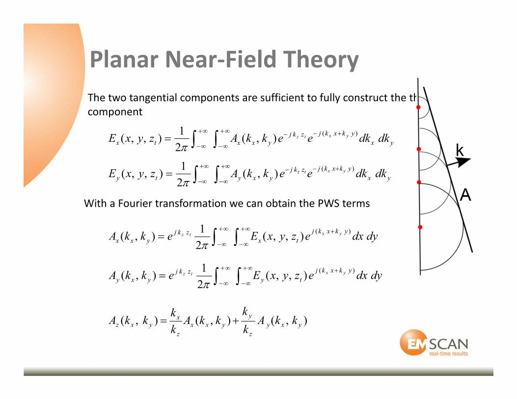
The two tangential components are sufficient to fully construct the third
component
With a Fourier transformation we can obtain the PWS terms
∫∫∞+
∞−
+∞+
∞−= dydxezyxEekkA
ykxkj
tx
zkj
yxxyxtz)(
),,(2
1),(
π
∫∫∞+
∞−
+∞+
∞−= dydxezyxEekkA
ykxkj
ty
zkj
yxyyxtz)(
),,(2
1),(
π
),(),(),( yxy
z
y
yxx
z
xyxz kkA
k
kkkA
k
kkkA +=
Planar Near-Field Theory
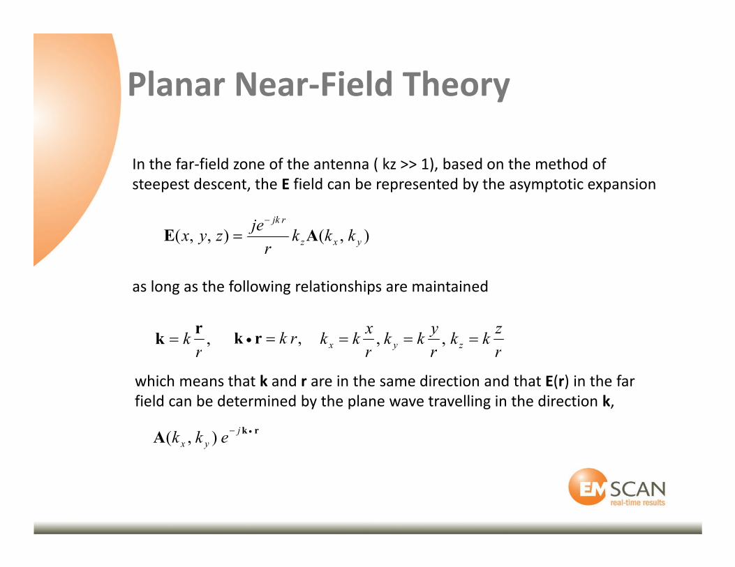
In the far-field zone of the antenna ( kz >> 1), based on the method of
steepest descent, the E field can be represented by the asymptotic expansion
as long as the following relationships are maintained
),(),,( yxz
rjk
kkkr
jezyx AE
−
=
,rkr
k = ,rk=• rkr
zkk
r
ykk
r
xkk zyx === ,,
which means that k and r are in the same direction and that E(r) in the far
field can be determined by the plane wave travelling in the direction k,
rk
A•− j
yx ekk ),(
Planar Near-Field Theory
Planar Near-Field Theory
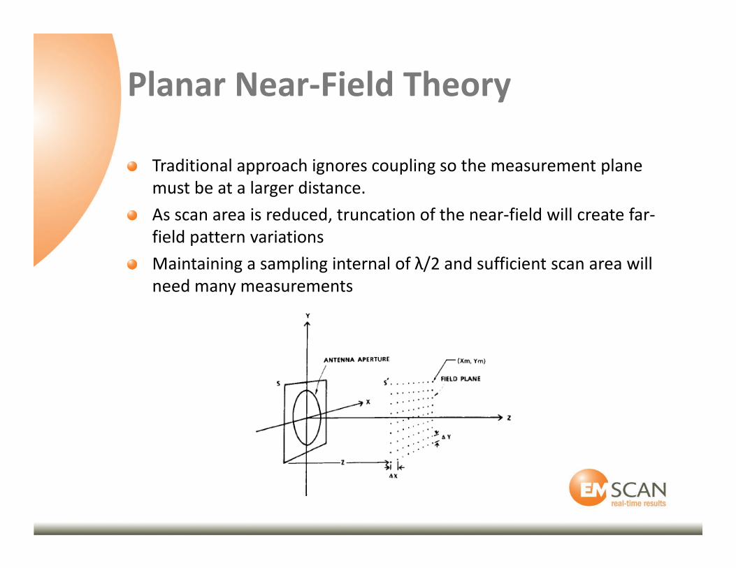
Traditional approach ignores coupling so the measurement plane
must be at a larger distance.
As scan area is reduced, truncation of the near-field will create far-
field pattern variations
Maintaining a sampling internal of λ/2 and sufficient scan area will
need many measurements
Planar Near-Field Theory
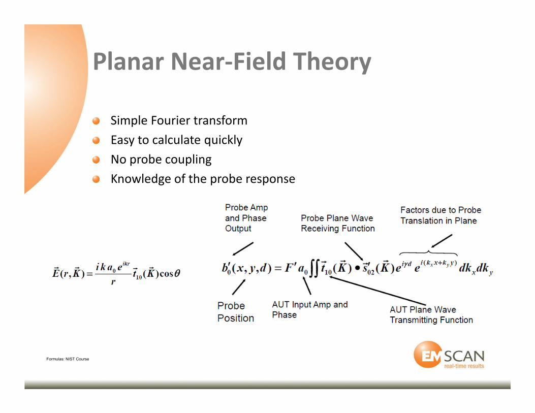
Simple Fourier transform
Easy to calculate quickly
No probe coupling
Knowledge of the probe response
Formulas: NIST Course
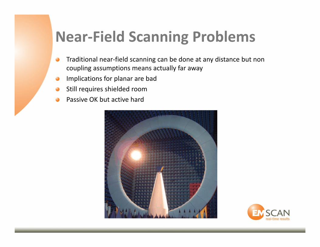
Traditional near-field scanning can be done at any distance but non
coupling assumptions means actually far away
Implications for planar are bad
Still requires shielded room
Passive OK but active hard
Near-Field Scanning Problems
Very-Near-Field Solution
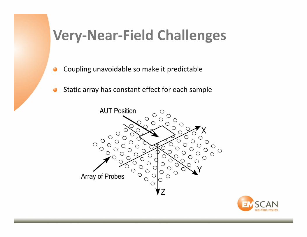
Very-Near-Field Challenges
Coupling unavoidable so make it predictable
Static array has constant effect for each sample
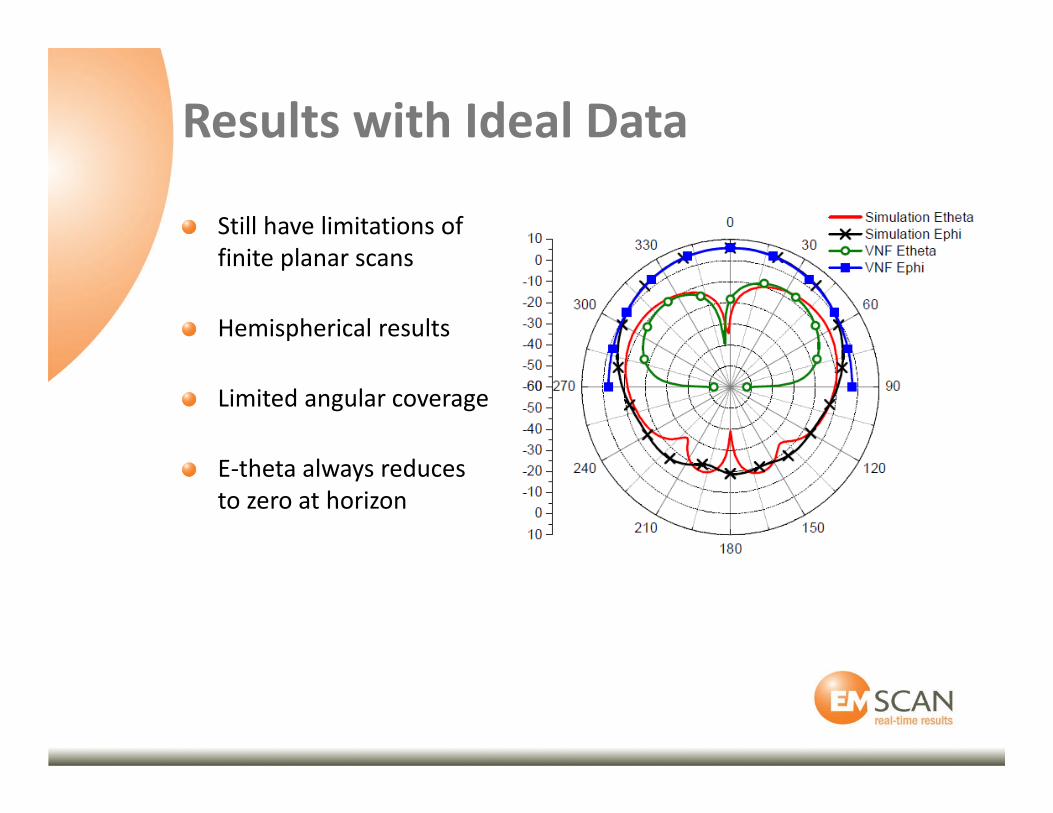
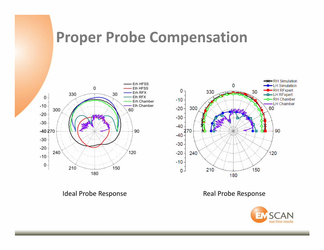
Results with Ideal Data
Still have limitations of
finite planar scans
Hemispherical results
Limited angular coverage
E-theta always reduces
to zero at horizon
-40
-30
-20
-10
0
0
30
60
90
120
150
180
210
240
270
300
330
-40
-30
-20
-10
0
Erh HFSS
Elh HFSS
Erh RFX
Elh RFX
Erh Chamber
Elh Chamber
Ideal Probe Response Real Probe Response
Proper Probe Compensation
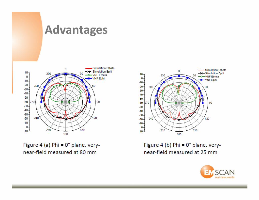
Advantages
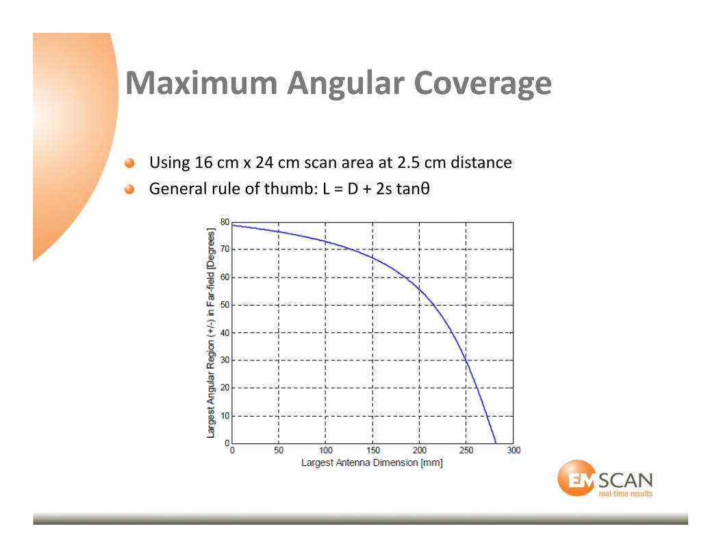
Maximum Angular Coverage
Using 16 cm x 24 cm scan area at 2.5 cm distance
General rule of thumb: L = D + 2s tanθ

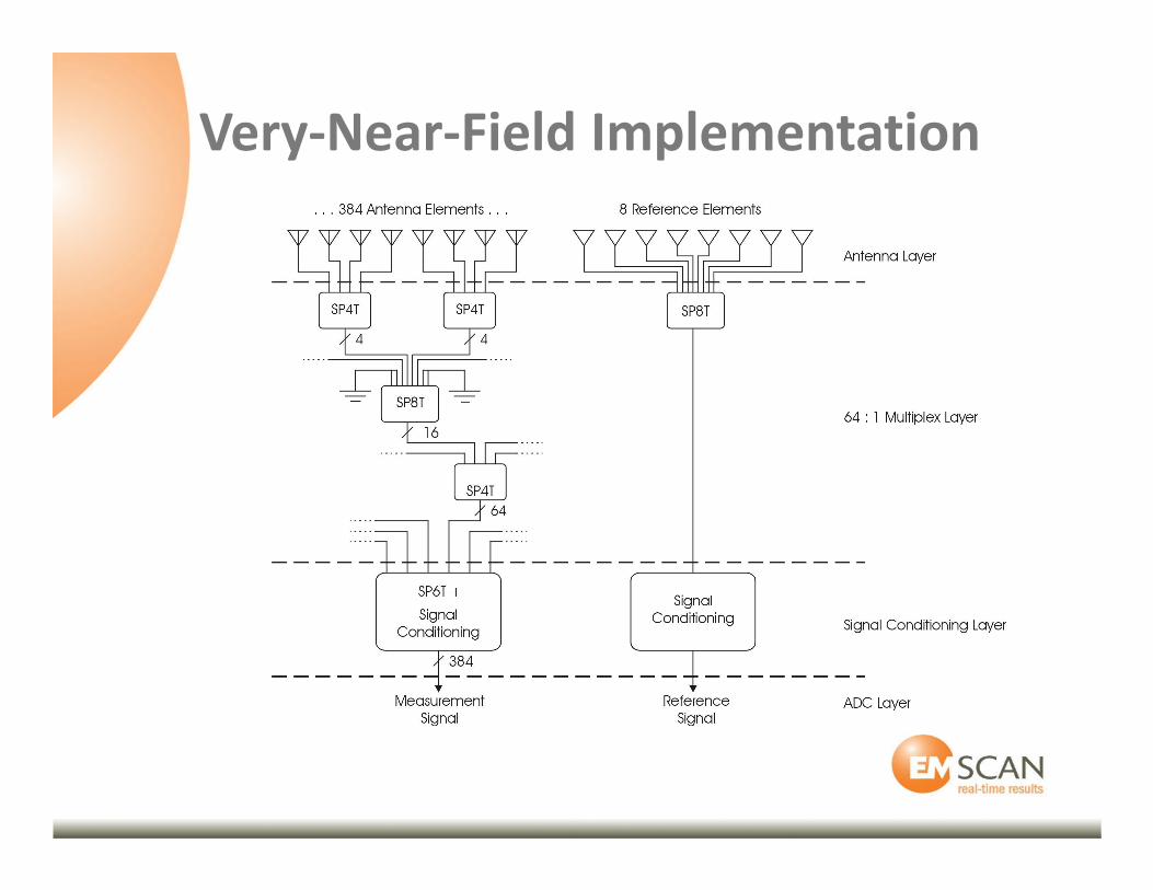
Very-Near-Field Implementation
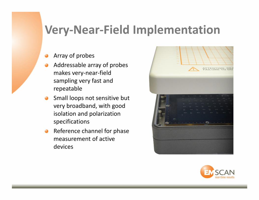
Very-Near-Field Implementation
Array of probes
Addressable array of probes
makes very-near-field
sampling very fast and
repeatable
Small loops not sensitive but
very broadband, with good
isolation and polarization
specifications
Reference channel for phase
measurement of active
devices
Very-Near-Field Implementation
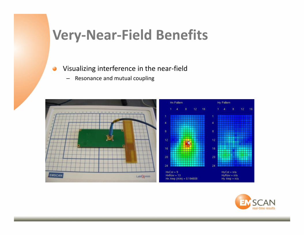
Very-Near-Field Benefits
Visualizing interference in the near-field
– Resonance and mutual coupling
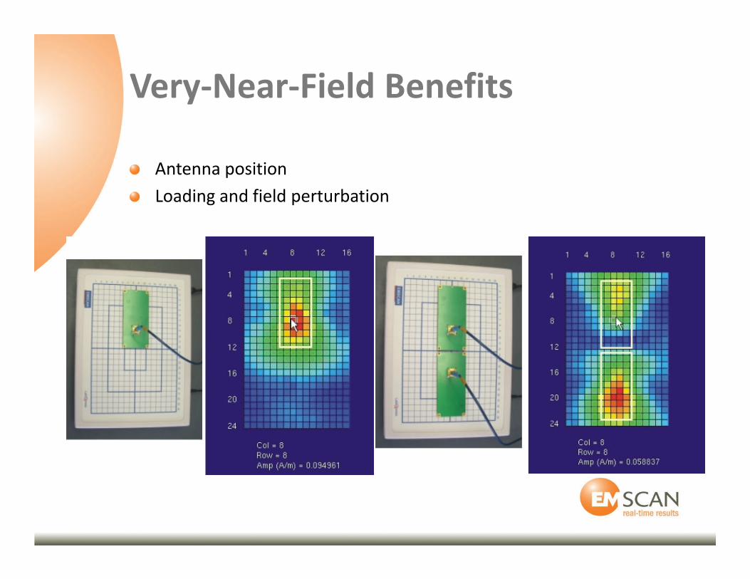
Very-Near-Field Benefits
Antenna position
Loading and field perturbation
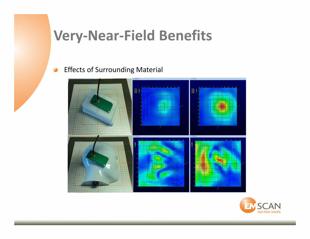
Very-Near-Field Benefits
Effects of Surrounding Material
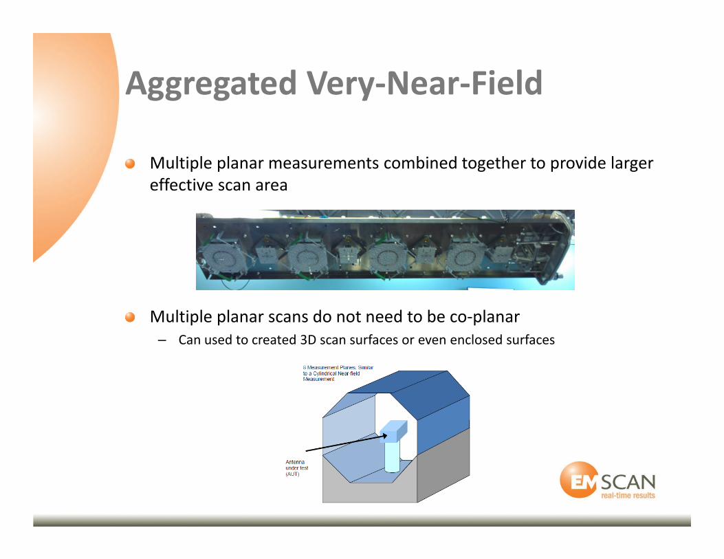
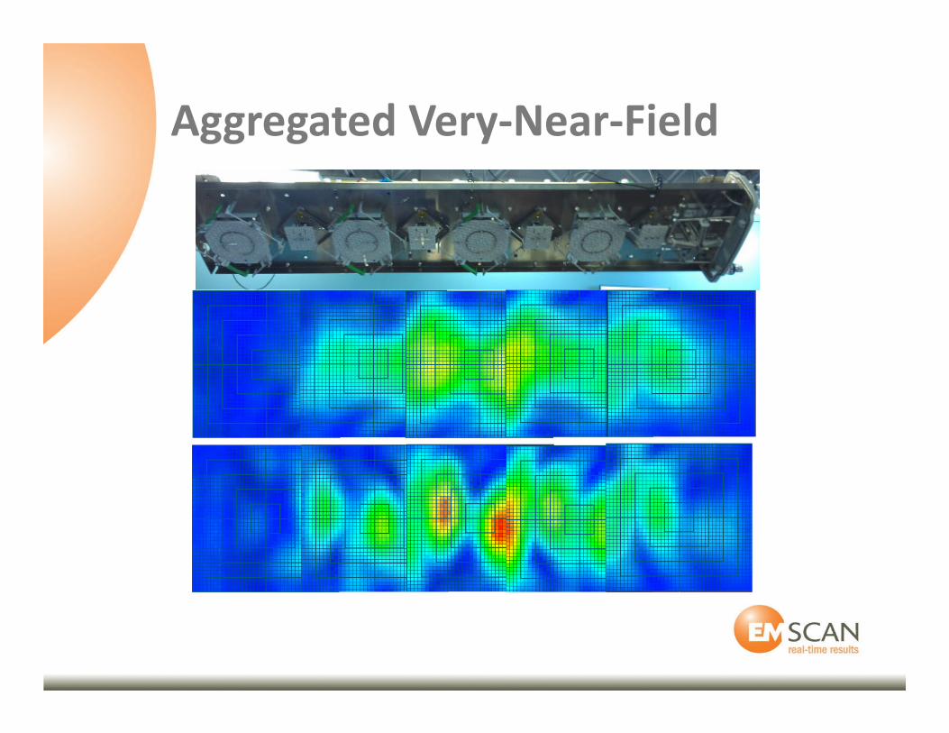
Aggregated Very-Near-Field
Multiple planar measurements combined together to provide larger
effective scan area
Multiple planar scans do not need to be co-planar
– Can used to created 3D scan surfaces or even enclosed surfaces
Aggregated Very-Near-Field
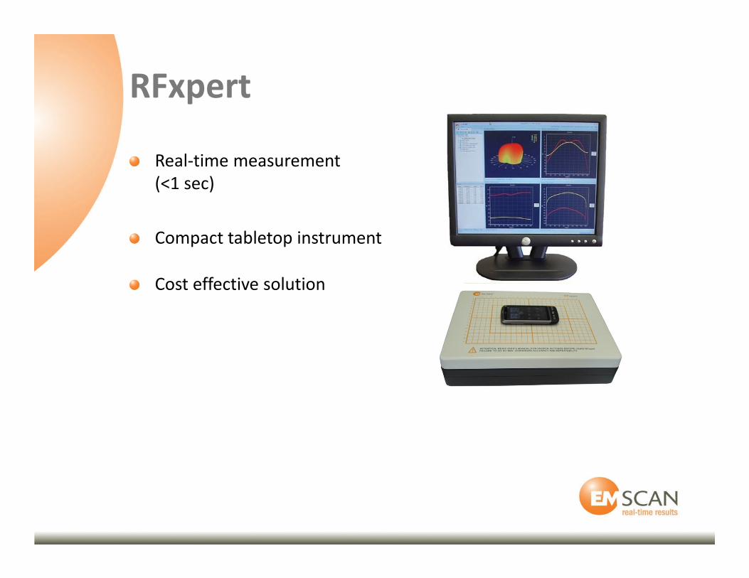
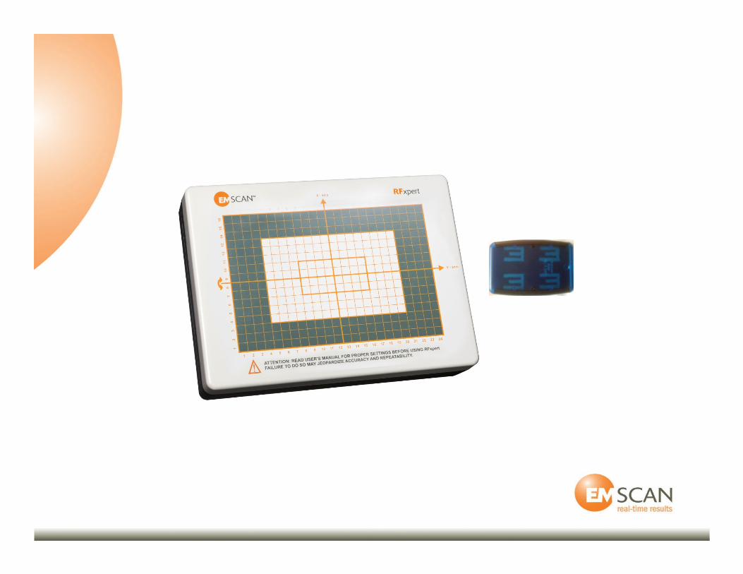
RFxpert
Real-time measurement
(<1 sec)
Compact tabletop instrument
Cost effective solution
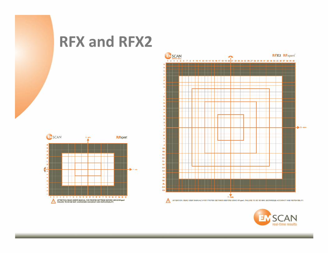
RFX and RFX2
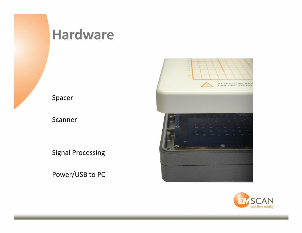
Hardware
Spacer
Scanner
Signal Processing
Power/USB to PC
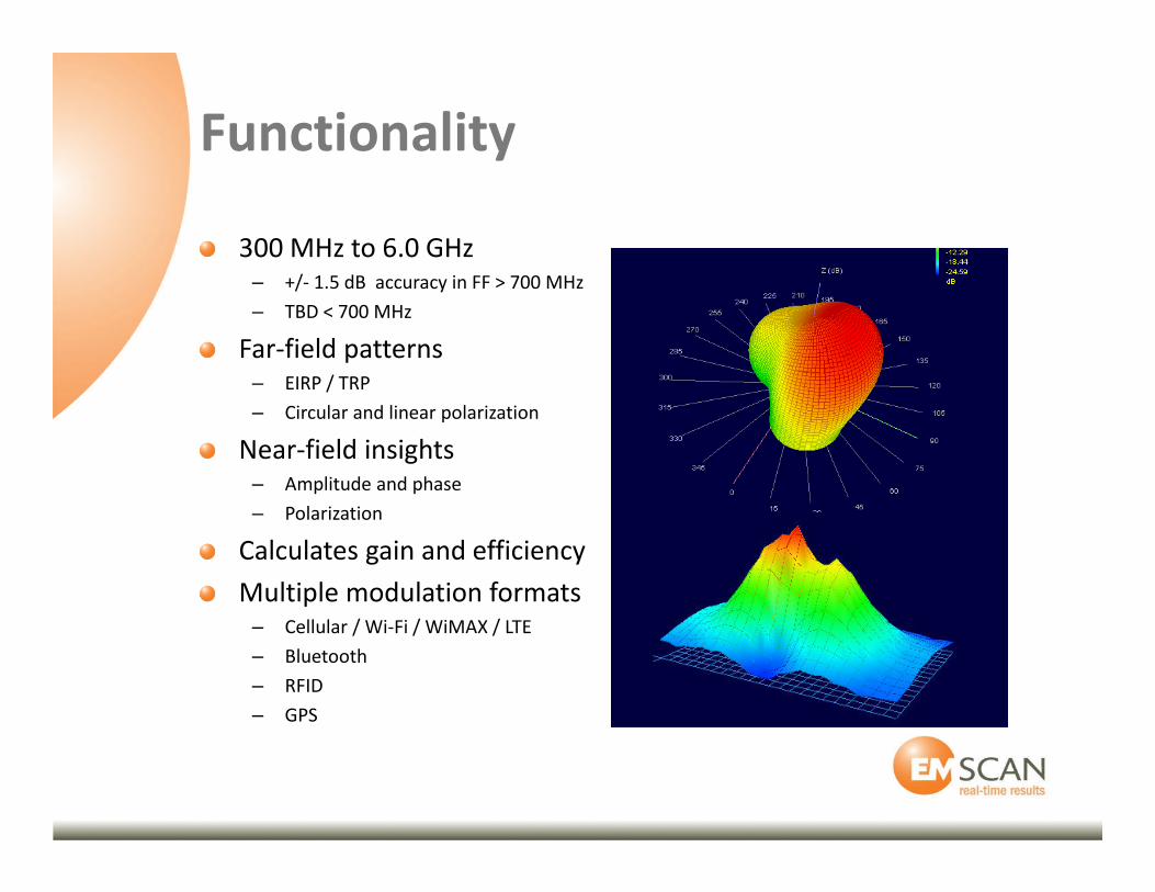
Functionality
300 MHz to 6.0 GHz– +/- 1.5 dB accuracy in FF > 700 MHz
– TBD < 700 MHz
Far-field patterns – EIRP / TRP
– Circular and linear polarization
Near-field insights– Amplitude and phase
– Polarization
Calculates gain and efficiency
Multiple modulation formats– Cellular / Wi-Fi / WiMAX / LTE
– Bluetooth
– RFID
– GPS

Technical Specifications
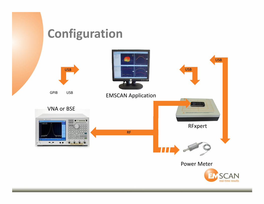
Configuration
USB USB
RFxpert
EMSCAN Application
VNA or BSE
Power Meter
USB
RF
GPIB USB
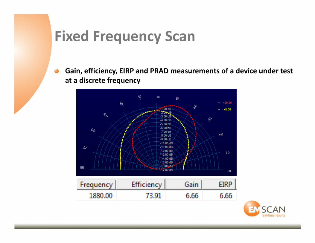
Fixed Frequency Scan
Gain, efficiency, EIRP and PRAD measurements of a device under test
at a discrete frequency
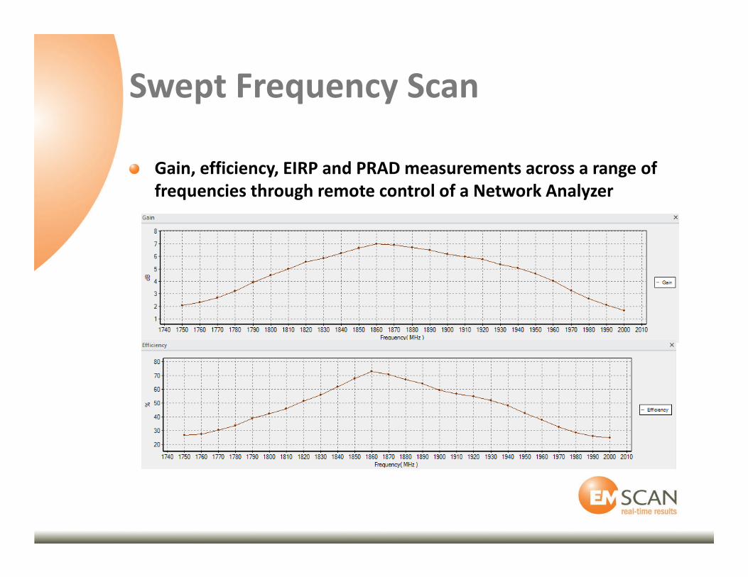
Swept Frequency Scan
Gain, efficiency, EIRP and PRAD measurements across a range of
frequencies through remote control of a Network Analyzer
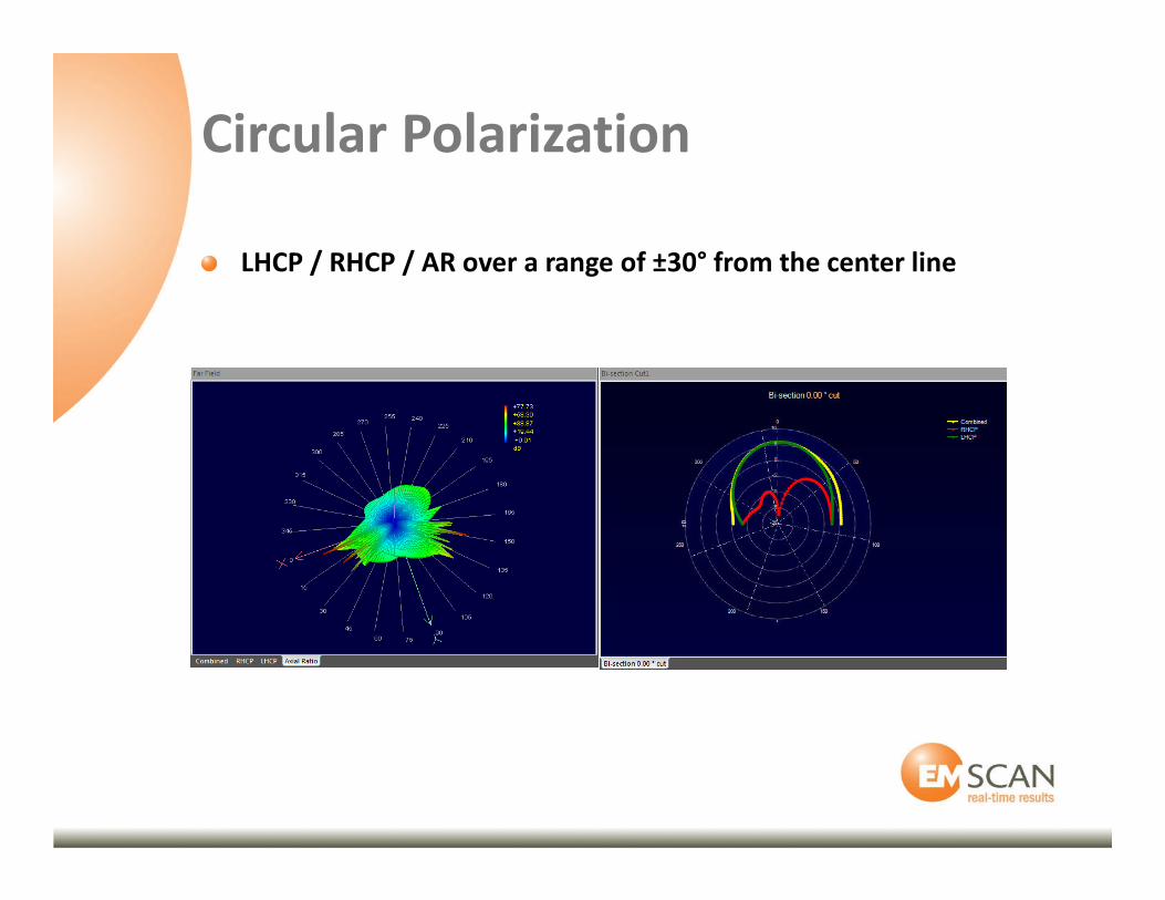
Circular Polarization
LHCP / RHCP / AR over a range of ±30° from the center line
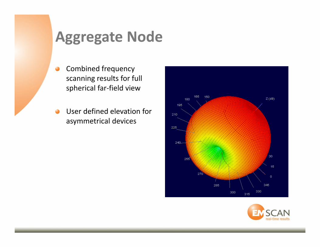
Aggregate Node
Combined frequency
scanning results for full
spherical far-field view
User defined elevation for
asymmetrical devices
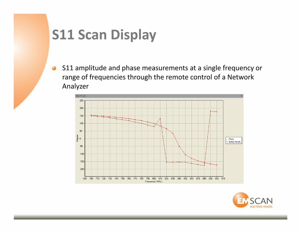
S11 Scan Display
S11 amplitude and phase measurements at a single frequency or
range of frequencies through the remote control of a Network
Analyzer
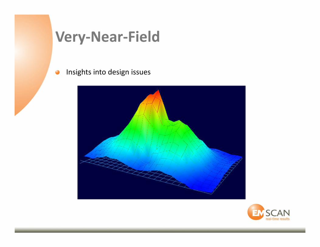
Very-Near-Field
Insights into design issues
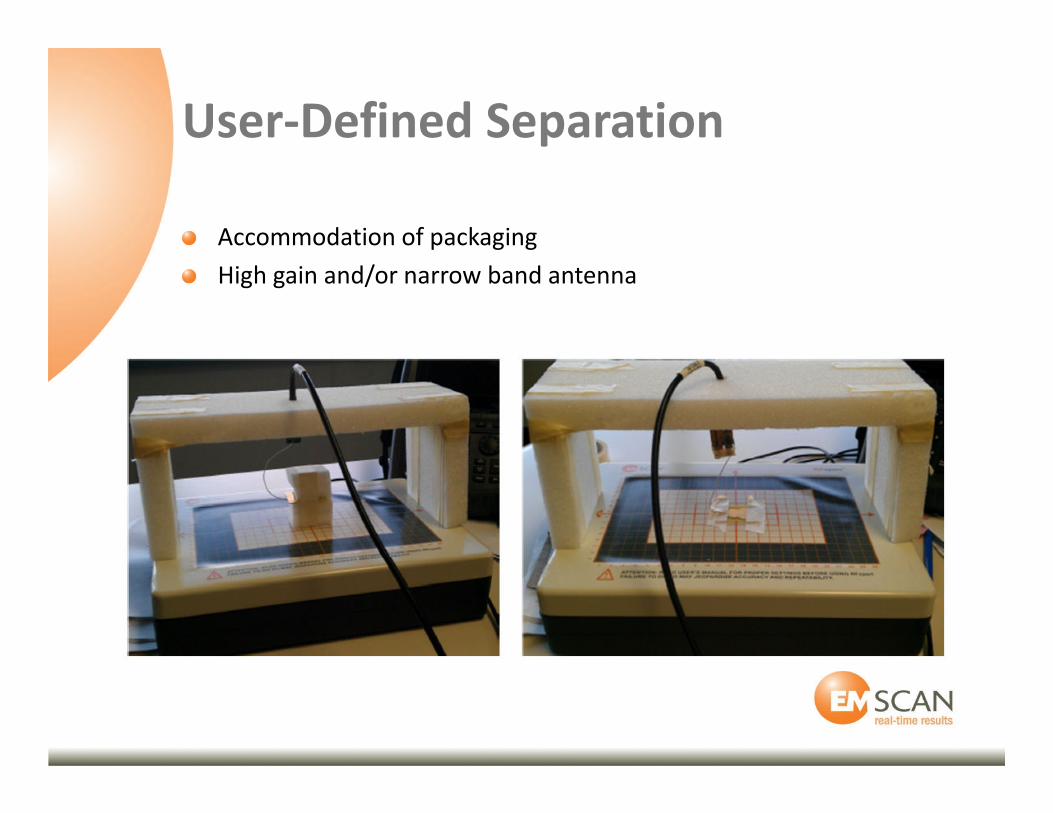
User-Defined Separation
Accommodation of packaging
High gain and/or narrow band antenna
Simulation
RFxpert Validation
Simulation
Agilent EDA simulation
Toyo corporation (EMSCAN Representative)
Tokyo, Japan
June 19, 2012
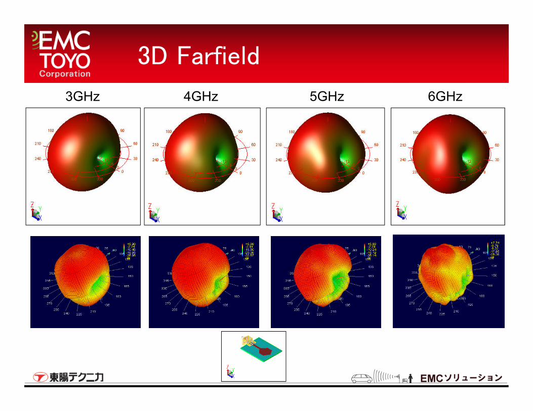
3D Farfield
3GHz 4GHz 5GHz 6GHz
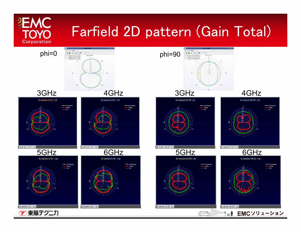
Farfield 2D pattern (Gain Total)
phi=0 phi=90
3GHz 4GHz
5GHz 6GHz
3GHz 4GHz
5GHz 6GHz
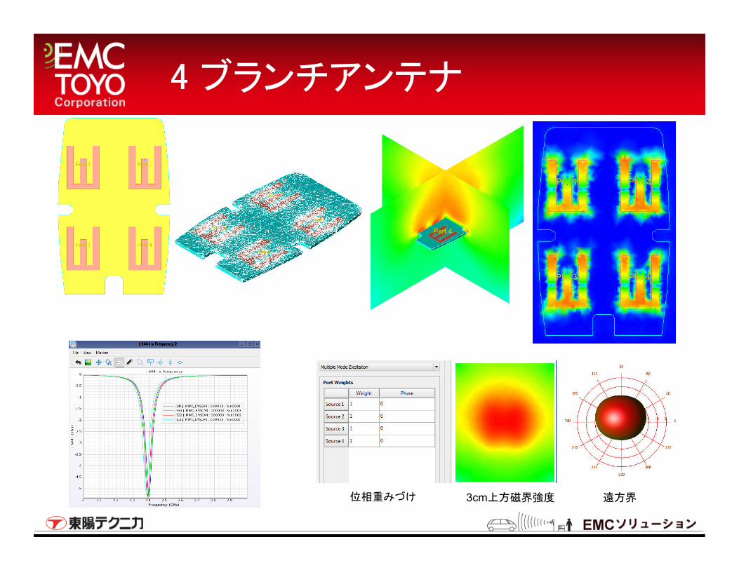
3cm上方磁界強度 遠方界位相重みづけ
4 ブランチアンテナ
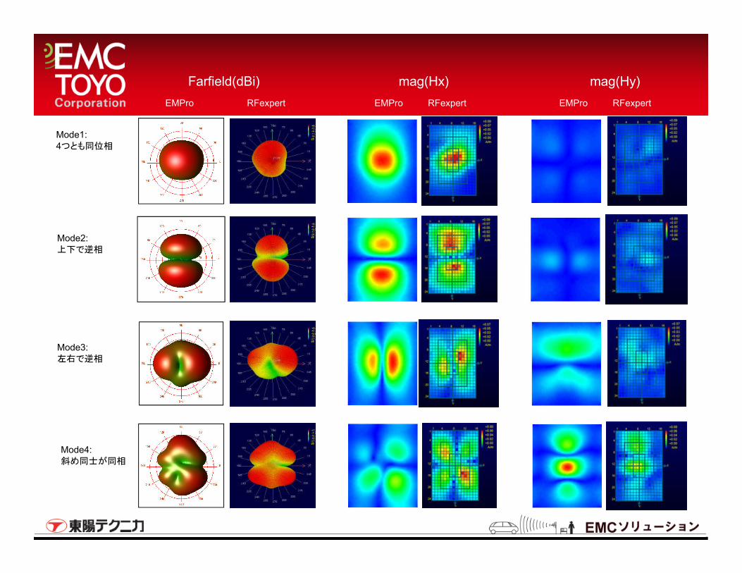
Mode3:
左右で逆相
Mode2:
上下で逆相
Mode4:
斜め同士が同相
Mode1:
4つとも同位相
mag(Hx) mag(Hy)Farfield(dBi)
EMPro RFexpertEMPro RFexpert EMPro RFexpert
Comparison with Chamber Results
RFxpert Validation
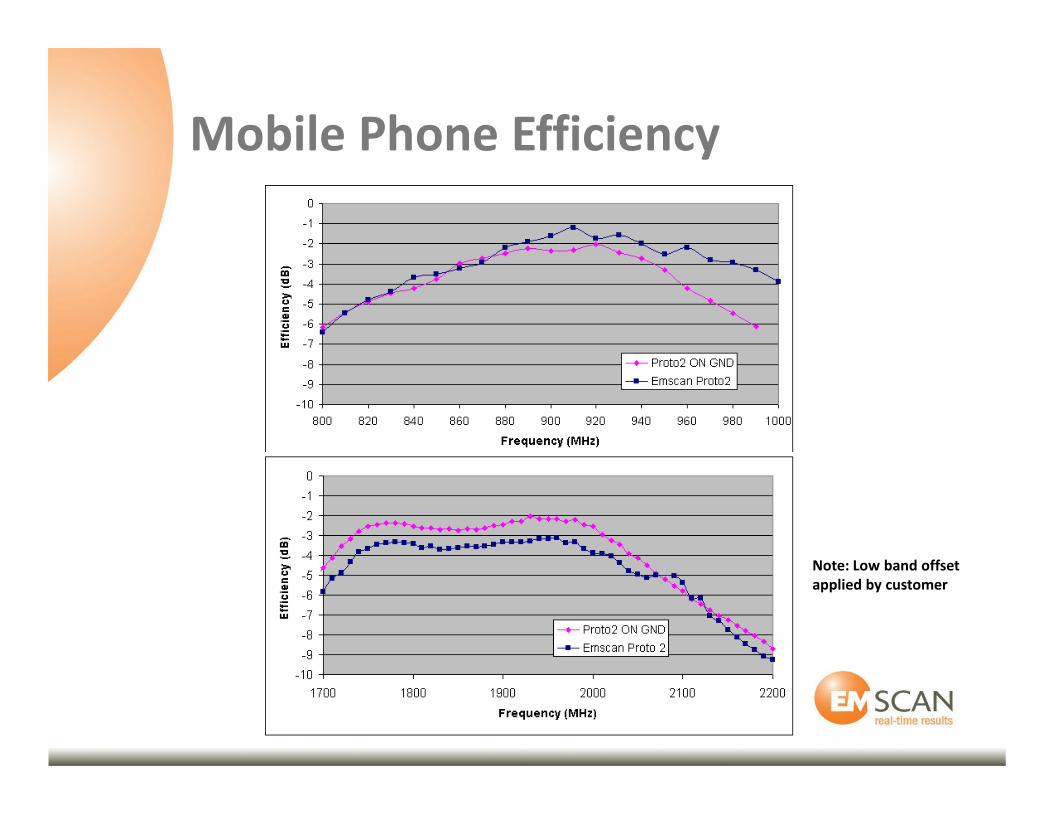
Note: Low band offset
applied by customer
Mobile Phone Efficiency
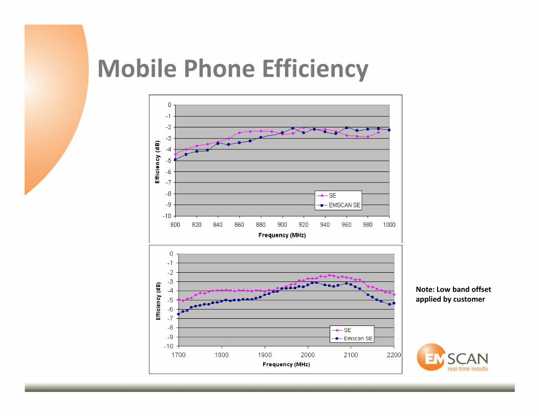
Note: Low band offset
applied by customer
Mobile Phone Efficiency
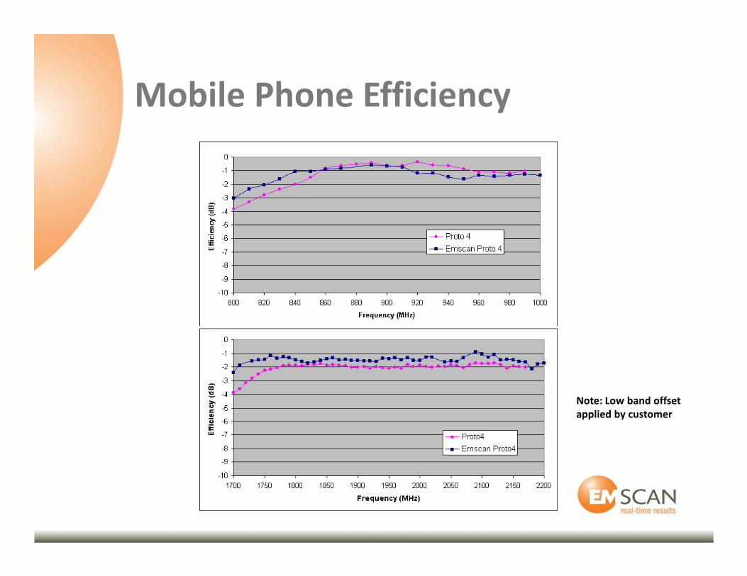
Note: Low band offset
applied by customer
Mobile Phone Efficiency
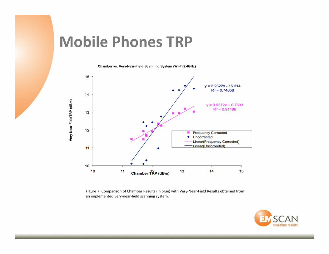
Very-Near-FieldTRP (dBm)
Figure 7: Comparison of Chamber Results (in blue) with Very-Near-Field Results obtained from
an implemented very-near-field scanning system.
Chamber vs. Very-Near-Field Scanning System (Wi-Fi 2.4GHz)
Mobile Phones TRP
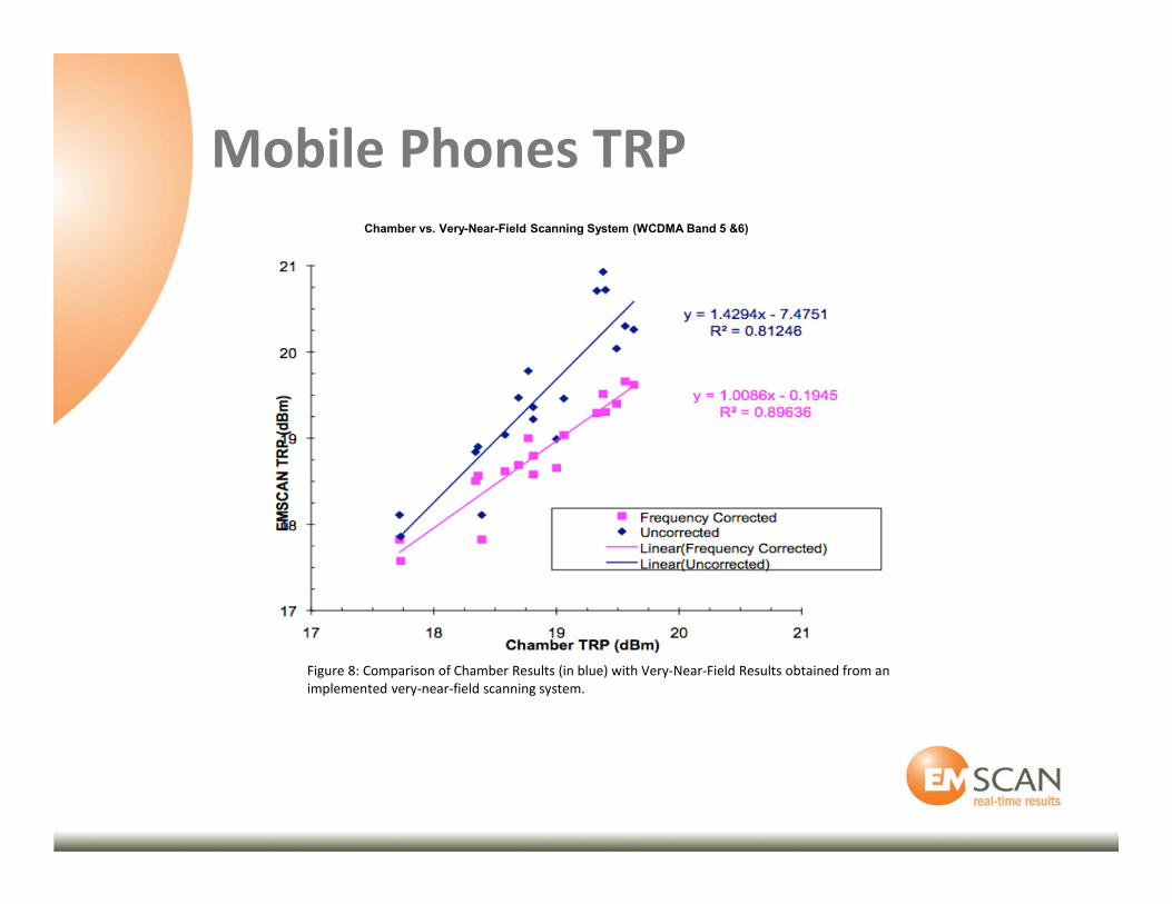
Figure 8: Comparison of Chamber Results (in blue) with Very-Near-Field Results obtained from an
implemented very-near-field scanning system.
Chamber vs. Very-Near-Field Scanning System (WCDMA Band 5 &6)
Mobile Phones TRP
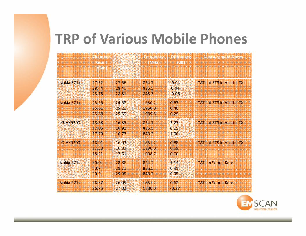
TRP of Various Mobile PhonesChamber
Result
(dBm)
EMSCAN
Result
(dBm)
Frequency
(MHz)
Difference
(dB)
Measurement Notes
Nokia E71x 27.52
28.44
28.75
27.56
28.40
28.81
824.7
836.5
848.3
-0.04
0.04
-0.06
CATL at ETS in Austin, TX
Nokia E71x 25.25
25.61
25.88
24.58
25.21
25.59
1930.2
1960.0
1989.8
0.67
0.40
0.29
CATL at ETS in Austin, TX
LG-VX9200 18.58
17.06
17.79
16.35
16.91
16.73
824.7
836.5
848.3
2.23
0.15
1.06
CATL at ETS in Austin, TX
LG-VX9200 16.91
17.50
18.21
16.03
16.81
17.61
1851.2
1880.0
1908.7
0.88
0.69
0.60
CATL at ETS in Austin, TX
Nokia E71x 30.0
30.7
30.9
28.86
29.71
29.95
824.7
836.5
848.3
1.14
0.99
0.95
CATL in Seoul, Korea
Nokia E71x 26.67
26.75
26.05
27.02
1851.2
1880.0
0.62
-0.27
CATL in Seoul, Korea
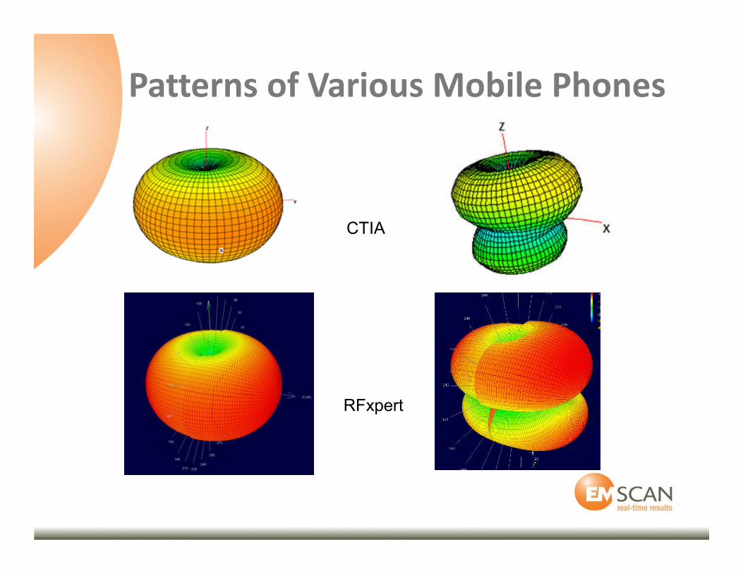
CTIA
RFxpert
Patterns of Various Mobile Phones
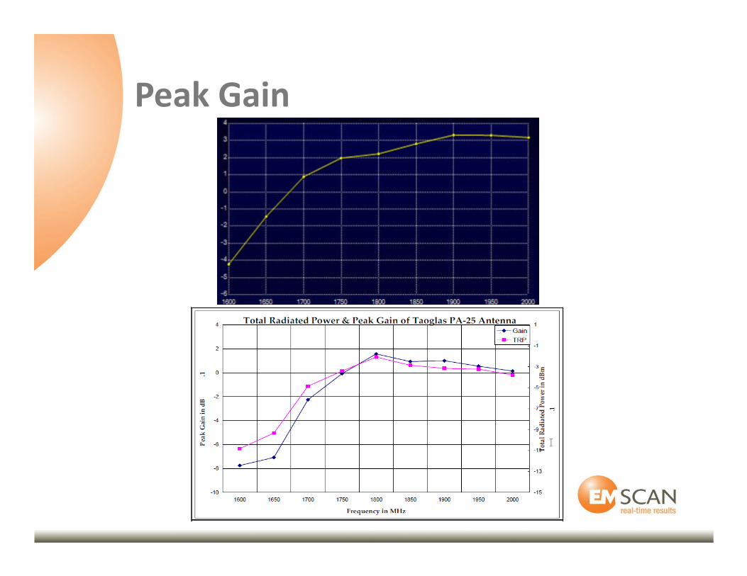
Peak Gain
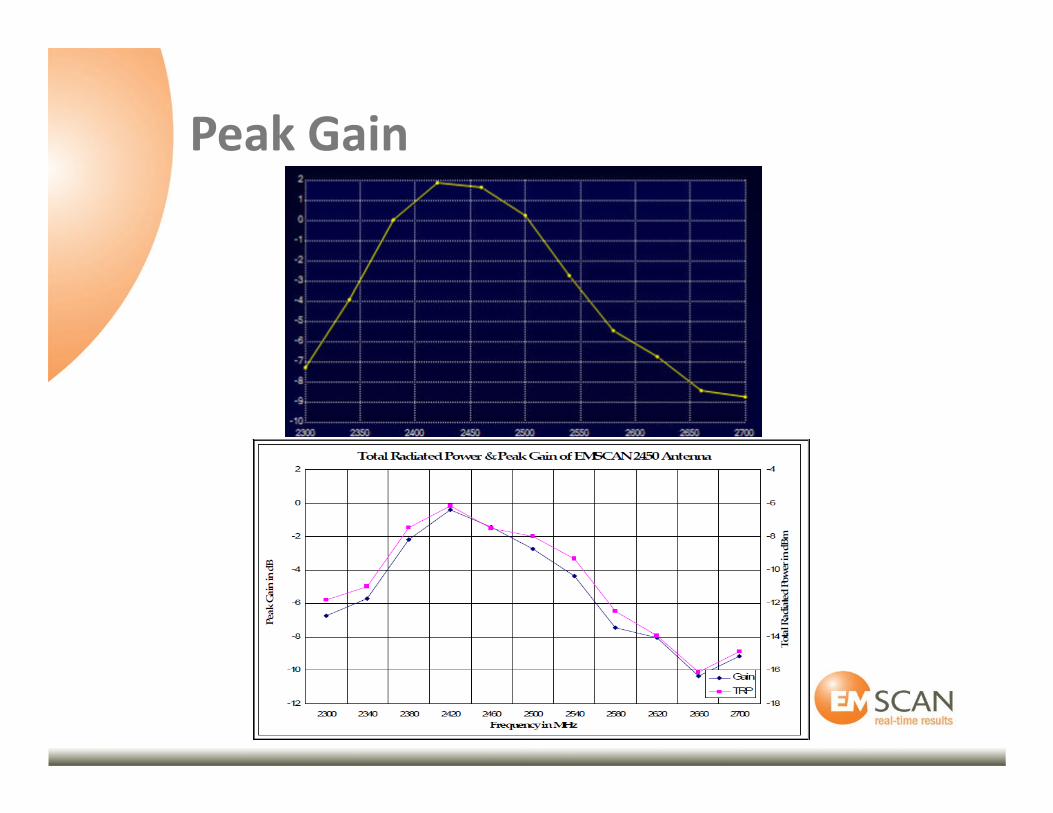
Peak Gain

Break

Test Applications
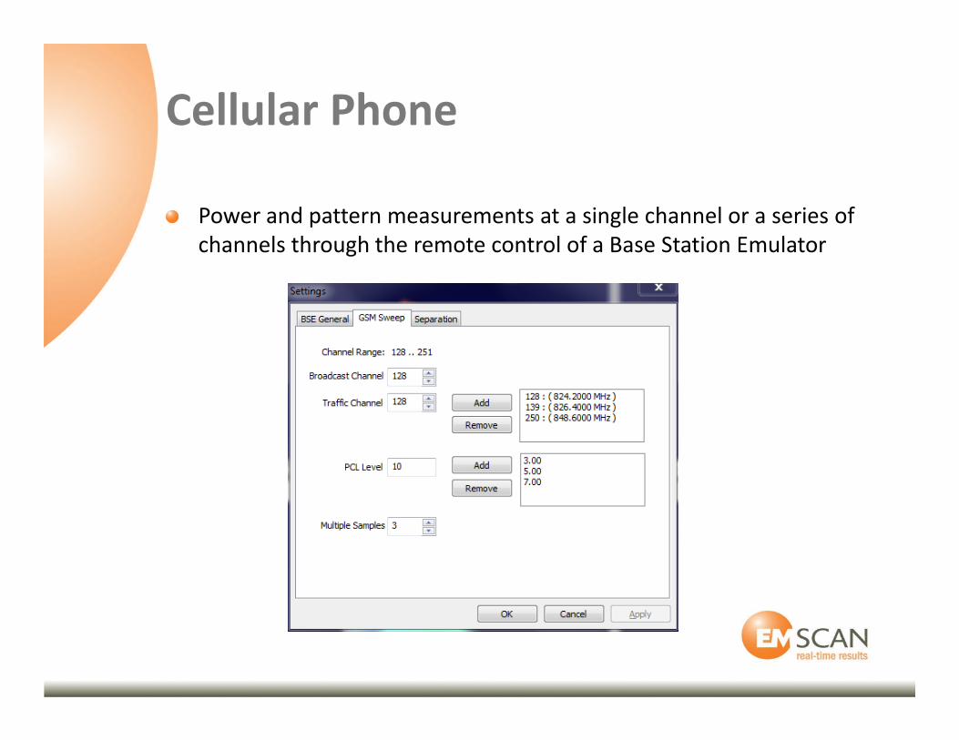
Cellular Phone
Power and pattern measurements at a single channel or a series of
channels through the remote control of a Base Station Emulator
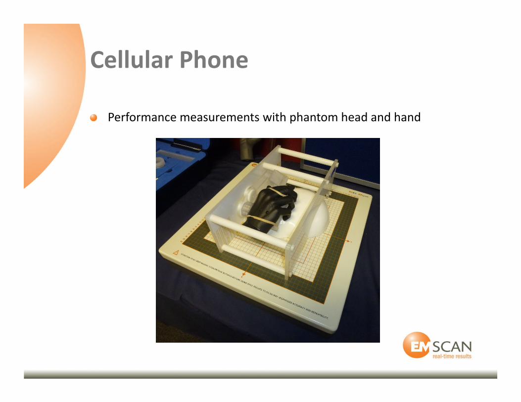
Cellular Phone
Performance measurements with phantom head and hand
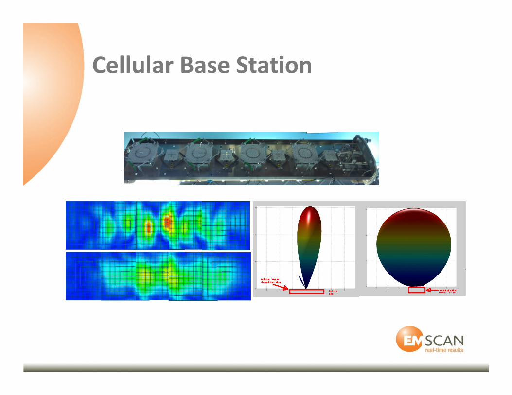
Cellular Base Station
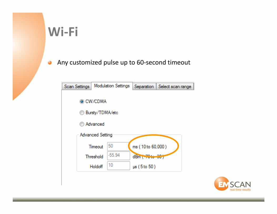
Wi-Fi
Any customized pulse up to 60-second timeout
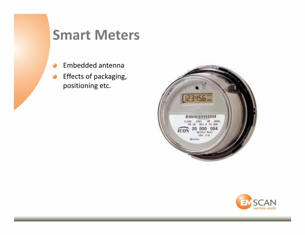
Smart Meters
Embedded antenna
Effects of packaging,
positioning etc.
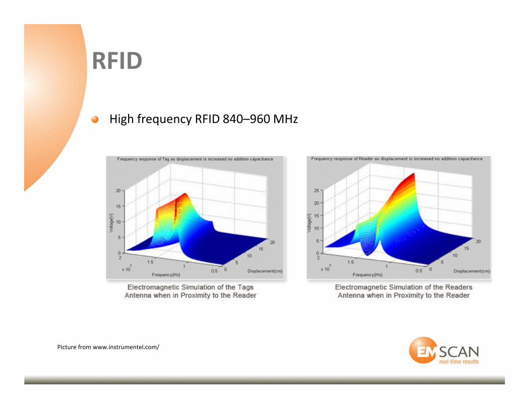
RFID
High frequency RFID 840–960 MHz
Picture from www.instrumentel.com/
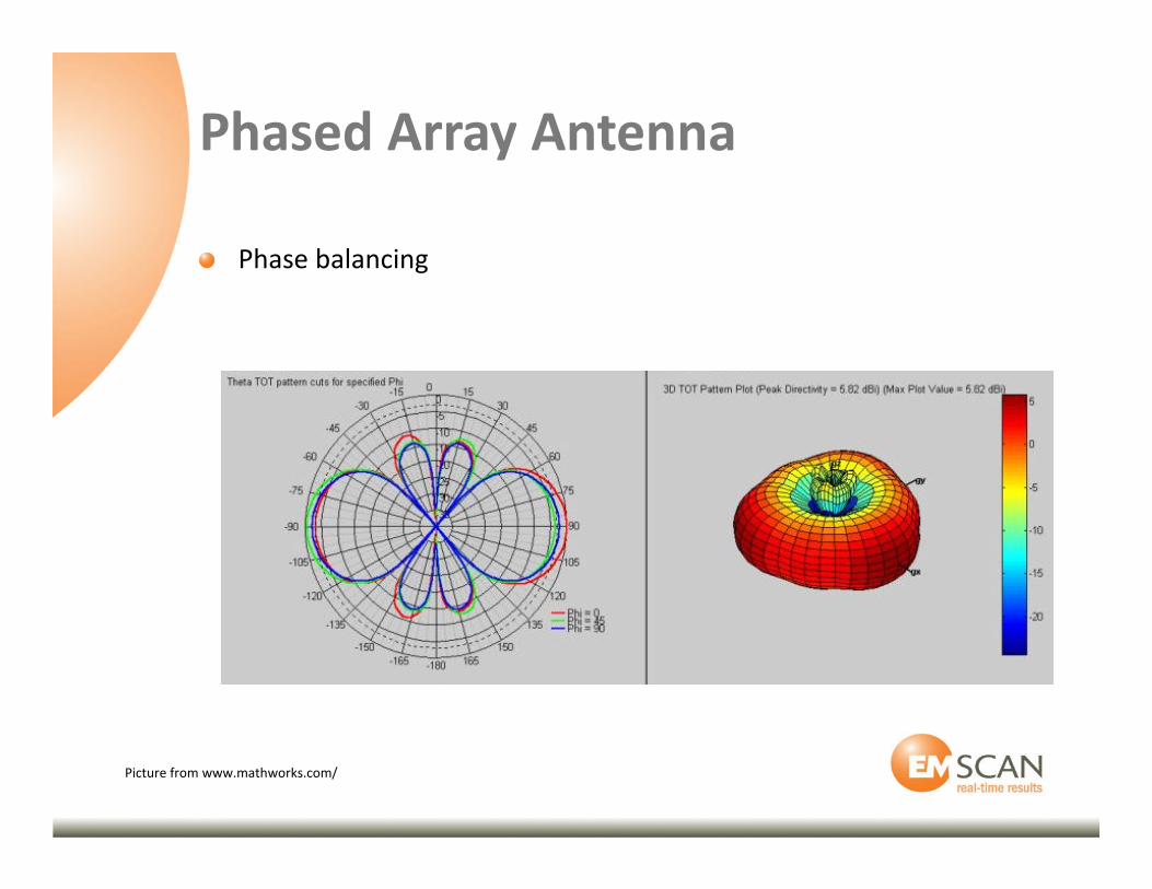
Phased Array Antenna
Phase balancing
Picture from www.mathworks.com/
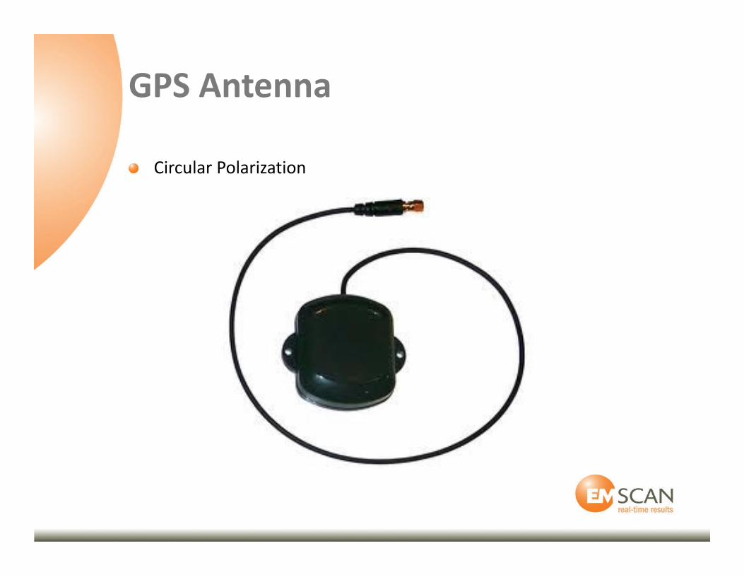
GPS Antenna
Circular Polarization
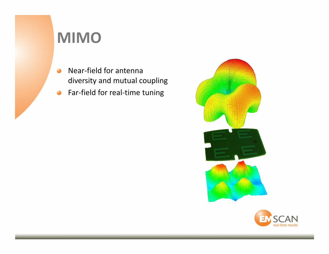
MIMO
Near-field for antenna
diversity and mutual coupling
Far-field for real-time tuning
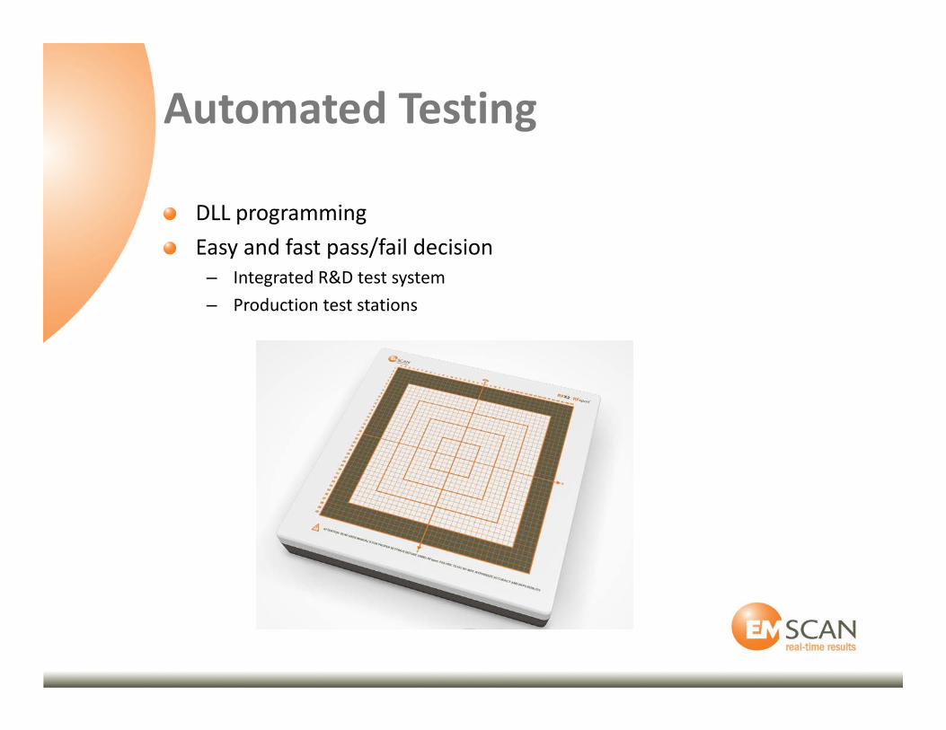
Automated Testing
DLL programming
Easy and fast pass/fail decision
– Integrated R&D test system
– Production test stations

Demonstration
Conclusion

Very-Near-Field Benefits
Ability to see surface
currents
Very fast scanning
Repeatable
No chamber
Low maintenance
Easy to use
RFxpert Advantages
Interaction effects in real-time
Near-field measurements
Fast and repeatable
Low CAPEX
Zero OPEX
RFxpert Value
Improved TTM and R&D productivity
– Test time reduction > 100 x
– Rapid design iteration, prototyping &
optimization
Reduced chamber CAPEX and OPEX
– Or a tool for each designer for better
productivity
Cost effective preparation to compliance

www.emscan.com
Thank You