1

Vertical Product Differentiation of Complementary Goods*

Georgi Burlakov

CERGE-EI†

Abstract

The paper introduces a model of vertical product differentiation as an extension of

Shaked and Sutton (1982) that allows for representation of the consumer demand for a bundle

of several complementary goods sold in separate markets. Two key differences are identified

in the equilibrium outcome. First, it is shown that the condition on market size derived by

Shaked and Sutton (1982) for having duopoly at equilibrium in an independent market might

not be sufficient to restrict down to two the equilibrium number of the possible bundles of

several complementary goods. Therefore, to have further decreased number of the salable

bundles, the mutual size of the markets must satisfy a more restrictive condition at which all

the complementary markets except one have a monopoly structure at equilibrium. Second, the

solution of the model implies that as long as one of the related markets has a monopoly

structure and its size exceeds half of its upper bound, this market would not be covered at its

pricing-stage equilibrium. Since the good sold in this market is a complement to the goods

sold in other related markets, however, the latter would not be covered at equilibrium, either.

The described result diverges from the one supported by Shaked and Sutton (1982) for a

single independent market where at the same conditions exactly two goods would have sales,

gain positive profits and cover the whole market at equilibrium.

Keywords: vertical product differentiation, complementary goods, market size, market

foreclosure

JEL classification: L11, L13, L15

* I would like to thank Eugen Kováč, Levent Çelik, Michael Kunin, Fabio Michelucci, Avner Shaked,

John Sutton, Krešimir Žigić (in alphabetic order) for valuable comments and helpful suggestions. † CERGE-EI is a joint workplace of the Center for Economic Research and Graduate Education, Charles

University in Prague, and the Economics Institute of the Academy of Sciences of the Czech Republic.

Address: CERGE-EI, Politickych veznu 7, Prague 11121, Czech Republic.

This paper was supported by the Grant Agency of the Charles Univeristy [Grantová agentura Univerzity Karlovy

v Praze], No. 0324/2010.

2

1. Introduction

Product differentiation is a main feature distinguishing Monopolistic Competition

from the Perfect Competition market structures.

It is common knowledge in economics that if two goods in a market differ in quality

their demand would be inelastic. At least a consumer would be willing to pay more for one of

the two qualities and therefore would continue preferring it even if the other quality is offered

at a slightly lower price. Therefore, product differentiation is generally agreed to be a source

of market power for the firms and implies imperfect competition among them.

One of the forms of product differentiation recognized by economists is the so-called

vertical product differentiation which is first described by Gabszewicz and Thisse (1979).

A key distinguishing feature of the models of vertical product differentiation is that all

consumers agree on which good is the best in the market, respectively which is second best

and so on, thus forming a common ranking of the goods based on their qualities. So, when

product qualities are vertically differentiated, they differ not by the specific consumer taste

each suits but by the extent to which any given quality is able to satisfy the consumer tastes as

a whole. All consumers prefer the product which serves them better to the one that serves

them worse even if the latter is offered at a slightly lower price.

What is specific about the markets with vertical product differentiation is that their

equilibrium outcome differs from the optimal result in markets with classical Chamberlinian

monopolistic competition structure. Even when barriers to entry are not present in a market

with vertical product differentiation, only finite number of potential market entrants could

make sales in equilibrium. They all earn positive profit and cover the market. Markets with

vertical product differentiation, minimal barriers to entry and still endogenously bounded

number of entrants that could coexist in equilibrium are known in industrial economics as

natural oligopolies due to Shaked and Sutton (1983).

This paper studies vertical product differentiation of goods which are complementary

though sold in different markets. More particularly, it makes a revision of a special market

equilibrium described by Shaked and Sutton (1982) at which as long as the market is

3

sufficiently narrow1, exactly two entrants will cover the market and still make positive profits

from selling their vertically differentiated products. The aim is to explore how this outcome

would differ if the goods offered by the two entrants are complementary to other goods

offered in a separate market.

In real world, there are a lot of examples of goods whose demand is affected by the

price of their separately sold complements.

A classical example of complementary goods from the basic economics textbooks2 is

washing machines and laundry detergents. As the price of the liquid detergent for automatic

laundry machines decreases, standard washing powder gets eventually obsolete. As a result,

non-automatic laundry machines might get also out of use because some low-income

consumers might still find the higher prices of the only available liquid washing detergents

unaffordable.

Similarly, not all toothpastes are best to use with an electric toothbrush. Even though,

dental studies3 show that if used properly, electric brushes have higher efficiency in plaque

and stain removal with any toothpaste, there are experts who warn against power brushing

with certain types of toothpastes. Because of the larger number of brush strokes per minute

use, electric toothbrushes have the risk to wear down teeth when used in combination with

high-abrasive toothpastes which are otherwise less harmless if applied by manual brushes.

Also, electric brushes tend to generate more foam if applied to standard toothpastes which

implies that less foamy dry pastes are more suitable for power brushing. Respectively, as the

price of dry low-abrasive toothpastes gets more affordable to larger share of population, they

might completely remove the old foamy high-abrasive pastes from the market. Afterwards,

however, some low-income consumers might find the higher price of the only available low-

abrasive toothpastes unaffordable and therefore stop brushing their teeth at all.

1 In the original work of Shaked and Sutton (1982), the size of the market is given by the variance of the

consumer incomes which are assumed to be uniformly distributed in that range. Later on, however, Tirole (1988)

shows that income could be considered just as an approximation of the consumer tastes for quality (see

Tirole, 1988, p.96). Respectively, in the model presented here, a preference is given to the utility functional form

suggested by Mussa and Rosen (1978) based on taste instead of on income parameter because it makes

computations simpler without loss of generality.

2 See Anderton, 2006, p.47.

3 Complete list of the scientific publications on the topic is available at the following web page:

http://eu.broxo.com/en/clinical_studies/complete_list.aspx

4

Another relevant example is the market for illuminants. With the appearance of the

energy-saving light bulbs, many households diverted their demand from the lamps with

standard bulbs to economize on the bill for electricity. However, for the households with low

bills for electricity, buying the more expensive light bulbs might not be reasonable. So, if the

energy-saving bulbs turn to be the only available in the market, households with low energy

consumption might be better-off if they drop electric lighting at all.

Last, it is also worth mentioning an example from the modern telecommunications

industry. The lower the price of mobile telecom services are, the larger becomes the number

of cell-phone users. However, the price of cell phones could still be too high for the low-

income consumers who would eventually stop using telecom services as standard fixed-line

phones get obsolete.

What is common for the examples above is that competition between an innovated

(high-quality) product and its standard (low-quality) precursor leads to decrease in their

prices. Respectively, if the market size is small enough the sales of the non-innovated product

might get efficiently foreclosed. This is a standard well-known outcome in the markets with

vertical product differentiation.

What is unusual in the examples given here, however, is that markets might remain

uncovered. This is because the described markets are not independent but instead the goods

sold in one market are complements to the goods sold in the other market. A product

purchased in a market cannot bring positive utility to the consumer if not combined with a

product from the other market. For instance, consumer gains little from buying a washing

machine if she has no detergent for it. Similarly, buying liquid detergent for automatic

laundry machine cannot help the consumer much if she has no automatic laundry machine.

Therefore, the size of both markets for washing powder and for laundry machines must be the

same. Nevertheless, the critical value of the size beyond which at most two goods could have

positive share differs among the markets because of the different weights the qualities of the

powder and the laundry machine have in the utility of their mutual consumption.

In other words, the range of incomes among the population of consumers buying both

washing detergents and laundry machines could imply such a market size which is large

enough for at most two types of laundry machines to be sold – automatic and non-automatic,

respectively. At the same time, however, this same market size could be too small for other

5

than liquid detergent to be sold in the market for washing detergents. As a result, liquid

detergent will be charged monopoly price which is above the reservation price of the low-

income consumers. Respectively, the latter will purchase neither a washing machine nor any

washing powder. Thus, both markets will remain uncovered.

The present paper suggests an extension of the model used by Shaked and

Sutton (1982) which allows for representation of the consumer demand for a bundle of several

complementary goods sold in separate markets. The solution of the extended model implies

that at particular market conditions an equilibrium outcome would exist where the bundle of

two innovated complementary products could monopolize their markets without covering

them. It has two evidential differences from the equilibrium solution of the single-product

model of Shaked and Sutton (1982).

First, since there are several markets, a good from one market could form a bundle

with any of the goods available in another market. So, the number of possible bundles in

which a good takes part increases both in the number of markets where its complements are

sold and in the number of complements sold in each market. Therefore, the restriction on the

market size which is derived by Shaked and Sutton (1982) as a sufficient condition for at most

two goods to have positive demand in a single market still allows for all the complements

available in another market to be sold as long as they could form bundles with the two goods

in the first market. In order to have not more than two bundles of complementary goods sold

in equilibrium, the condition on market size needs to be increasingly restrictive as the number

of goods in a bundle grows. Nevertheless, the restriction has a limit and does not increase

incessantly as the number of the markets for complementary goods tends to infinity.

Second, the buying decision of the consumers with low willingness to pay for quality

depends not only on the price of the low-quality good sold in a single market but is also

determined by the prices of all the goods that enter together with it in the low-quality bundle.

To illustrate this, in the example with the market for washing detergents, let the related market

for laundry machines is considered as independent and its size is in a particular narrow range

which in compliance with Shaked and Sutton (1982) ensures exactly two goods with positive

market shares at equilibrium. Then, the expectations would indeed be two qualities of

washing machines, say automatic and non-automatic, to be sold at equilibrium and the market

to be covered. In the market for detergents, however, provided that the qualities of its goods

6

have higher weight in consumer’s utility, the same market size would imply that only the best

good (e.g. liquid detergent) could have a positive demand. Respectively, the liquid detergent

would be optimal to be charged the monopoly price which would make not only it but also the

bundles in which it takes part prohibitively expensive for the low-taste consumers. The latter

would not be willing to pay the monopoly price of the only detergent available even if it is of

the best (i.e. liquid) quality possible. This would make pointless for them also the purchase of

a washing machine. In turn, this would drive down to zero the demand for the low-quality

good in the market for washing machines. So, only the best washing machine will be sold and

counter to the single-market expectations no market would be covered at equilibrium, but still

all markets would have monopoly structure even without barriers to entry.

The paper is organized as follows. Section 2 introduces the extended model of vertical

product differentiation adjusted to reflect the consumer demand for bundles of complementary

goods. Section 3 states the general condition for at most two bundles to have sales in

equilibrium and discusses the resulting equilibrium outcome in case of two related markets.

Section 4 concludes.

7

2. The Model

The model that is going to be introduced for the purpose of the analysis in the present

paper is an extension of the model suggested by Shaked and Sutton (1982). It is based on the

same three-stage non-cooperative game in which first firms make an entry decision, then

entrants choose quality and finally they compete in prices. The payoff of the firms that decide

to enter the market in the first stage is given by their profit less an infinitesimally small cost of

entry 0 . For simplicity, it is assumed that firms have no production costs. Non-entrants

earn zero payoffs.

What is new in the present model is that it considers not just a single market but

several markets for complementary goods. Each firm is assumed to sell only one good. So, it

is identified not only by the quality of the good it produces but also by the market in which

this good is offered.

For example, let’s have two markets and denote them by A and B. There are m

entrants in market A and n entrants in market B. In each market let firms be identified by the

market rank of the quality of the good that each of them offers, as shown below:

mAfAfAf ....21 (1)

where iAf denotes the value that consumers assign to a mutually-agreed mix of

characteristics of the product of type A based on which it is ranked at i-th place by quality;

FAfF i , mi ,...,1 ;

nBgBgBg ....21 (2)

where jBg denotes the value that consumers assign to a mutually-agreed mix of

characteristics of the product of type B based on which it is ranked at j-th place by quality;

GBgG j , nj ,...,1 .

8

Respectively, firms’ profits (revenues) are represented by the following expressions:

A

m

AAAA ppDp ,...,1111 (3)

………………………………..

A

m

A

i

AA

i

A

i

A

i pppDp ,...,,...,1

……………………………….

A

m

AA

m

A

m

A

m ppDp ,...,1

where:

A

i - profit (revenue) of good ranked i-th by quality in market A, mi ,...,1

A

iD - the demand for good ranked i-th by quality in market A, mi ,...,1

A

ip - the price of good ranked i-th by quality in market A, mi ,...,1

B

n

BBBB ppDp ,...,1111 (4)

………………………………..

B

n

B

j

BB

j

B

j

B

j pppDp ,...,,...,1

……………………………….

B

n

BB

m

B

m

B

m ppDp ,...,1

where:

B

j - profit (revenue) of good ranked j-th by quality in market B, nj ,...,1

B

jD - the demand for good ranked j-th by quality in market B, nj ,...,1

B

jp - the price of good ranked j-th by quality in market B, nj ,...,1

9

The demand for a good in each of the two markets is given by the sum of the market

shares of the bundles in which the good takes part:

n

j

ij

A

i DD1

, mi ,...,1 (5)

m

i

ij

B

j DD1

, nj ,...,1 (6)

where ijD is used to denote the demand for bundle AiBj consisting of the i-th best

quality good in market A and the j-th best quality good in market B.

The demand for bundles ijD is derived from the consumers’ optimal choices. Each

consumer chooses to purchase the bundle which maximizes her individual consumer surplus

given by the standard utility function introduced by Mussa and Rosen (1978):

jjiiijijijij BgpAfppU , (7)

where:

- taste parameter4 by which consumers are identified; is assumed to be uniformly

distributed on an interval

ij - quality of bundle AiBj

jiij BgAfpp , - price of bundle AiBj as a function of the qualities of the goods

in it

ii

A

i Afpp - price of good Ai as a function of its quality5

)]([ jj

B

j Bgpp - price of good Bj as a function of its quality

4 could be considered as a measure of the marginal utility of quality (Mussa and Rosen, 1978) or consumer’s

income (Shaked and Sutton, 1982). It is straightforward to show that the two are equivalent

(see Tirole, 1988, p.96).

5 To simplify the notation, the prices of goods are denoted by

A

ip mi ,...,1 if they are of type A and by

B

jp nj ,...,1 if they are of type B.

10

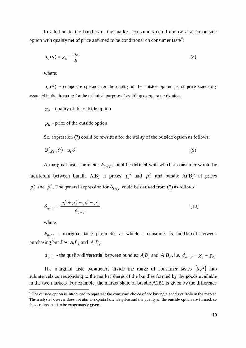
In addition to the bundles in the market, consumers could choose also an outside

option with quality net of price assumed to be conditional on consumer taste6:

O

OO

pu )( (8)

where:

)(Ou - composite operator for the quality of the outside option net of price standardly

assumed in the literature for the technical purpose of avoiding overparametrization.

O - quality of the outside option

Op - price of the outside option

So, expression (7) could be rewritten for the utility of the outside option as follows:

OO uU , (9)

A marginal taste parameter ''/ jiij could be defined with which a consumer would be

indifferent between bundle AiBj at prices A

ip and B

jp and bundle Ai’Bj’ at prices

A

ip ' and B

jp ' . The general expression for ''/ jiij could be derived from (7) as follows:

''/

''

''/

jiij

B

j

A

i

B

j

A

i

jiijd

pppp (10)

where:

''/ jiij - marginal taste parameter at which a consumer is indifferent between

purchasing bundles ji BA and '' ji BA

''/ jiijd - the quality differential between bundles ji BA and '' ji BA , i.e. ''''/ jiijjiijd

The marginal taste parameters divide the range of consumer tastes , into

subintervals corresponding to the market shares of the bundles formed by the goods available

in the two markets. For example, the market share of bundle A1B1 is given by the difference

6 The outside option is introduced to represent the consumer choice of not buying a good available in the market.

The analysis however does not aim to explain how the price and the quality of the outside option are formed, so

they are assumed to be exogenously given.

11

between the upper bound of the taste parameters’ range and the marginal taste parameter

between the best and second best bundle. Let the latter be A1B2. Then, the expression for best

bundle’s market share is as follows:

12/1111 D (11)

The expression for the market share of the worst bundle differs dependent on whether the

market is covered or not. For instance, let the worst bundle available be A1B2. Then, its

market share is as follows.

OO

OD

/12/1212/11

/1212/11

12 i.e.market covered-nongiven ,

i.e.market coveredgiven ,

(12)

where:

O/12 - taste parameter with which a consumer would be indifferent between the

lowest quality bundle A1B2 and the outside option i.e. between buying and not buying in the

market.

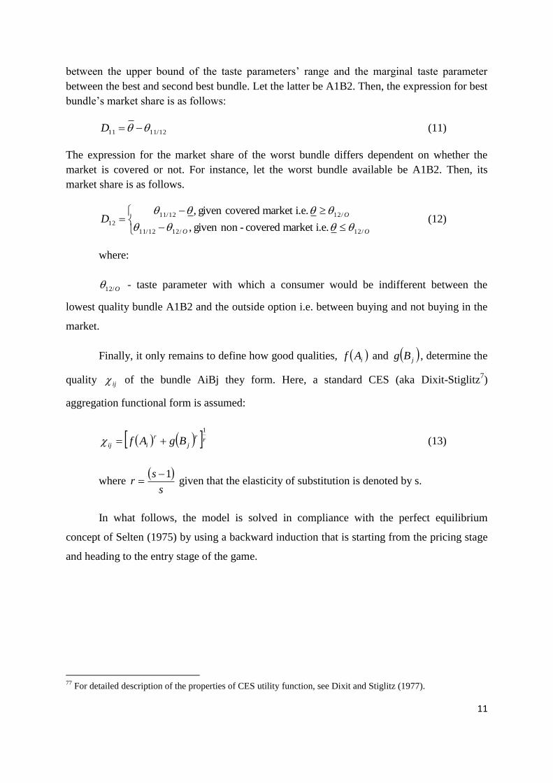
Finally, it only remains to define how good qualities, iAf and jBg , determine the

quality ij of the bundle AiBj they form. Here, a standard CES (aka Dixit-Stiglitz7)

aggregation functional form is assumed:

rr

j

r

iij BgAf1

(13)

where

s

sr

1 given that the elasticity of substitution is denoted by s.

In what follows, the model is solved in compliance with the perfect equilibrium

concept of Selten (1975) by using a backward induction that is starting from the pricing stage

and heading to the entry stage of the game.

77

For detailed description of the properties of CES utility function, see Dixit and Stiglitz (1977).

12

3. Solution for the optimal outcome at market size allowing for at

most two bundles with positive sales at equilibrium

The analysis of the subgame equilibrium in the pricing stage follows closely the

methodology of Shaked and Sutton (1982).

First, nm potential bundles are assumed to co-exist in equilibrium. However, this

is not sufficient for unambiguous explicit-form representation of the profit-maximization

problems in (3) and (4). As shown in (5) and (6), distinct from the case with a single market

for independent goods, when two markets for complementarily bundled goods are considered,

each good could be sold as a part of several bundles. Therefore, the ranking of the bundles

could vary dependent on how the qualities of the goods that form them relate to each other.

Nevertheless, a general condition on the quality differences between the bundles could be set

such that independent on their ranking, a system of first-order optimality equations for profit

maximization could be derived which is compatible with the solution results of Shaked and

Sutton (1982). The very condition and its direct implication are stated in proposition 1 below.

To facilitate the statement of proposition 1, let a subset of bundles based on A1 be better

than A2B1 and denote their number by k, nk ,1 . Similarly, let denote by l the number of bundles

based on A2 which are better than the superior of the two bundles A3B1 and A1Bk+1, nl ,1 .

Respectively, the optimal demand for bundle A1Bj kj ,...,1 is denoted by

jD1 , given that no

bundle A1Bj nkj ,..., has positive demand. Analogously,

jD2 denotes the optimal demand for

bundle A2Bj kj ,...,1 , given that no bundle A2Bj nlj ,..., has positive demand.

Proposition 1. Let the price-elasticity of demand for the bundles based on goods A1

and A2 fulfill the following conditions:

1

1

1

1

1

n

kj

j

k

j

j

k

D

D

(14)

13

1

1

2

1

2

n

lj

j

l

j

j

l

D

D

(15)

Then, for any pricing subgame equilibrium involving nm potential bundles in the

market, the following relationship between marginal taste parameters will hold:

1/111/231/221/1 4,42 mjmkllk Max for any nj ,...,2,1 (16)

Proof: see Appendix A

To make the sense of expressions (14) and (15) more intuitive, note that the price-

elasticities of their left-hand sides are both decreasing in the quality differences ''/1 jijd

between the bundles A1Bj for nkj ,...,1 and their neighbors by quality rank:

n

kj

j

An

kj jij

n

kj

j

A

A

n

kj

j

k

D

p

dD

p

p

D

1

1

1

1 ''/1

1

1

1

1

1

11

(17)

n

lj

j

An

lj jij

n

lj

j

A

A

n

lj

j

l

D

p

dD

p

p

D

1

2

2

1 ''/2

1

2

2

2

1

21

(18)

Hence, as smaller is the quality differential between the (n-k) bundles based on A1 that

are worse than A2B1, the more likely it would be condition (14) to hold. Similarly, as smaller

is the quality differential between the (n-l) bundles based on A2 that are worse than the

superior of A3B1 and A1Bk+1, the more likely it would be for the inequality in (15) to be

valid. To generalize, conditions (14) and (15) imply that low-quality bundles must differ less

distinctly each from another than high-quality bundles which is in fact a reasonable

assumption. Usually, high-quality innovative goods are harder to imitate than low-quality

generic products. As a result the competition between the less distinguishable bundles based

on the same good of type A but containing lower-quality goods of type B is stronger and their

demand is more price-sensitive.

In other words, given that conditions (14) and (15) hold, to make both top-quality and

bottom-quality bundles based on a good of type A salable, the price of that good must be

lower than in the case when only the top-quality bundles have positive market share.

14

Respectively, imagine that profit maximization requires from the producer of a good of

type A to charge it a (lower) price at which not only the top-quality but also the bottom-

quality bundles based on this good would have positive demand. Then, since the demand

function is strictly decreasing in price, the demand for the top-quality bundles at this (low)

equilibrium price cannot be smaller than the same demand at any other (high) price at which

only the top-quality bundles are sold. Therefore, when conditions (14) and (15) hold, the

values of the marginal taste parameters that define the borders of the demand for the k top-

quality bundles based on good A1 and the l top-quality bundles based on good A2 cannot get

any closer each to another than the minimal difference between them given by the inequality

in (16).

Straight from the expression in (16), a restriction could be imposed on the market size

so that at most goods A1 and A2 would have a positive market share in market A at

equilibrium:

4

(19)

This result replicates exactly the respective condition derived for single market by

Shaked and Sutton (1982). However, to restrict the equilibrium number of bundles with

positive market share to maximum two, it is not sufficient just to restrict down to two the

number of the goods in market A. In the case with two connected markets considered here,

the restriction of the maximal equilibrium number of goods in market A to two still allows to

form up to (2xn) bundles with the n goods in market B. Hence, as long as 1n , more

restrictive condition than (19) needs to be introduced for at most two bundles to have positive

market share in equilibrium. Furthermore, the larger is the number of the connected markets,

the stronger should also be the required restriction on the market size. The relationship

between the number of the goods in a bundle and the degree of restrictiveness of the

corresponding condition on market size from below is rigorously stated in the proposition that

follows:

15

Proposition 2. Let X be the number of the markets for complementary goods forming

a set of bundles satisfying the requirements of proposition 1 adjusted for X markets. Then, for

any pricing subgame equilibrium involving all possible bundles that can be formed from the

goods in the market, at most two bundles (the top two) will have a positive market share at

equilibrium as long as the following condition on market size holds8:

X

xx

112

1 (20)

Proof: see Appendix B

The economic intuition that stands behind proposition 2 is illustrated in figure 1

below. The larger is the number of connected markets, the larger would also be the number of

possible combinations in which the goods sold in these markets could be bundled.

Respectively, the only way the number of salable bundles could be restricted down to two is

to decrease the number of goods with positive market share in equilibrium, so that there are at

most two combinations in which they could be bundled. Particularly, this implies that the

restrictive condition on market size must be such that in one market at most two goods could

have a positive market share while on all the rest of the markets only a single good could be

sold in equilibrium. Then, the two combinations that could be sold at most will differ only by

the good they contain from the former (duopoly) market while the goods from the rest of the

(monopoly) markets will be the same for any of the bundles.

8 Note that the right-hand side has a limit of

2

1 as the number of goods in a bundle tends to infinity:

2

1

2

1

2

1lim

11

11

xx

X

xxX

.

16

On figure 1, the restrictive conditions on market size are depicted by arrows. Each

arrow divides the goods in each market into two groups. The goods under the arrow are the

ones that have no chance to have positive demand in equilibrium if the condition by which the

arrow is labeled holds. The goods above the arrow are the ones that could have positive

demand in equilibrium if the condition in the arrow by which the arrow is labeled holds. The

higher is an arrow, the more restrictive is the condition by which it is labeled.

Figure 1: Relationship between the number of the connected markets and the degree of

restrictiveness of the condition on market size for at most two bundles to have positive

markets shares in equilibrium

Note that the larger is the number of the markets the higher needs to be the arrow

corresponding to the condition which must hold in order up to two bundles to be salable in

Market …

…

…

…

…

…

…

Market B

B1

B2

…

Bn

Market C

C1

C2

…

Ch

Market Z

Z1

Z2

…

Zy

Market A

A1

A2

…

Am

mequilibriuat bundles ...2 toup ,4 yhn

mequilibriuat bundles ...21 toup ,83 yh

mequilibriuat bundles ...211 toup ,167 y

mequilibriuat bundles 2...111 toup ,21

1

X

x

x

17

equilibrium. This is because more markets are required to have only a single good i.e.

monopoly at equilibrium.

For example, when there is only a single independent market A, the condition

suggested by Shaked and Sutton (1982) is sufficient because it is not required for the market

to have monopoly structure. Duopoly is also acceptable in market A.

When there are two connected markets, A and B, the condition on size of an

independent market as derived by Shaked and Sutton (1982) is too weak and cannot reduce

the equilibrium number of bundles to maximum of two. Duopoly in market A would imply up

to n2 possible combinations in which the goods with positive chance to be sold at

equilibrium could be bundled. Ignoring market A to consider only market B as independent

would imply the incorrect expectation that at most two goods could have positive market

share in equilibrium. In fact, their number could be up to n but n might be larger than two.

Therefore, the maximum of two bundles requires more restrictive condition. Namely, this is

the condition by which is labeled the next arrow from above. It only allows for monopoly

structure of market A while at most duopoly could still occur in market B.

If there are three connected markets, that is a good of market C enters a bundle

together with its complements in markets A and B, also the size of market B should be further

restricted within a range corresponding to a monopoly structure. Thus, with each additional

connected market X, more and more markets are needed to have a monopoly structure in

order maximum of two bundles to be salable at equilibrium. In turn, a more restrictive

condition on market size must hold which corresponds to a higher-leveled arrow on figure 1.

In what follows, the case of two markets, A and B, will be considered with sizes

assumed to satisfy the condition in (20) for X=2 i.e. 8

3 . It remains to show how the

equilibrium outcome in the pricing stage changes compared to the particular case of single

independent market with vertical differentiation described by Shaked and Sutton (1982).

The critical factor for the difference in equilibrium outcomes between the case with

one independent market and the case of two markets for complementary products is the

implication of condition (20) for having monopoly in market A when it is connected with

market B.

18

Given only one entrant in market A, the standard equilibrium outcome in case of

monopoly suggests that the market cannot be covered as long as its size exceeds the half of its

upper bound i.e. 2

. In other words, the single entrant in market A is better-off of

charging its good a high price at which only the high-taste consumers are willing to purchase

it than to serve all consumers at a low price.

Then, however, low-taste consumers who find the good in market A too expensive for

them to afford buying it would lose incentive to do shopping in market B as well. This is

because they have positive utility of good B only conditional on using it in combination with

good A. So, market B would also be uncovered at equilibrium. Moreover, as stated in

proposition 3 below, the resulting competitive pressure on good B2 would be so strong that it

would not be able to sustain positive market share even by pricing at a cost.

Proposition 3. Let the condition of proposition 1 holds and let the common size of

markets A and B satisfy the restriction 28

3

. Then, at equilibrium only the best good

in each market, A1 in market A and B1 in market B, will have positive market shares but

market will not be covered by them.

Proof: see Appendix C

As a final outcome, good B2 is driven out from the market and only B1 is sold in

market B. So, both markets, A and B, would be uncovered and have a monopoly structure at

equilibrium. This outcome differs from the equilibrium result in case of a single independent

market. As demonstrated by Shaked and Sutton (1982) if market B is independent, both goods

B1 and B2 will have positive market shares, gain positive profits and serve all consumers at

equilibrium.

The subgame equilibrium of the quality-choice stage is derived explicitly in

appendix D. There it is shown that the profits of both A1 and B1 are strictly increasing in their

qualities. So, the optimal quality choices are given by the corner solution at which A1 and B1

are assigned the highest possible quality values, F and G , respectively. All the rest

19

2 nm potential entrants gain zero revenue (i.e. negative profits of ) independent of

their quality choice. Therefore, it is optimal for them not to enter the market in the first stage.

The conclusion is that at the particular perfect subgame equilibrium corresponding to

the backward solution presented in the paper, only the firms offering goods A1 and B1 enter

their markets, after which they assign their products the best qualities and charge them the

monopoly price. In turn, the market is not covered, that is the low-taste consumers find both

goods prohibitively expensive and therefore prefer to abstain from them than to pay their high

monopoly prices.

20

4. Conclusion

In the presented paper an extended model of Shaked and Sutton (1982) is introduced

as tool for analysis of the competition outcome in a market for vertically differentiated goods.

What makes this market distinct from the one considered originally is that its goods are

complements to goods sold in other markets. As a result, the decisions firms make in a market

are not independent but influenced by the decisions of the firms in the rest of the related

markets. Respectively, two key differences are identified in the equilibrium outcome.

First, since each good has one or more complements its demand depends not only on

its price and quality but also on the prices and qualities of the other goods with which it could

be consumed. Therefore, the condition on market size derived by Shaked and Sutton (1982),

for duopoly at equilibrium might not in fact restrict down to two the equilibrium number of

the bundles. For instance, in a pair of related markets with two goods in each, it is possible up

to four bundles to have a positive market share at equilibrium. Therefore, to decrease their

number down to two, the mutual size of the markets must satisfy a more restrictive condition

at which all markets but one have a monopoly structure with just a single good sold at

equilibrium.

Second, as long as at least one of the related markets has a monopoly structure and its

size exceeds half of its upper bound, this market would not be covered at its pricing stage

equilibrium. Since the good sold in this market is a complement to the goods sold in other

related market, however, the latter cannot be covered at equilibrium, either. Furthermore,

resulting competitive pressure would turn the second market to monopoly. This equilibrium

outcome is very different from the one described by Shaked and Sutton (1982) for a single

independent market where two goods would have positive market share, gain positive profits

and cover the whole market at equilibrium.

The analysis presented in the paper could be continued in a further research on the

topic. Particularly, an interesting question to be answered is whether equilibrium would exist

at which two firms would enter in each market given a weaker restriction on the market size.

Accordingly, it would be reasonable to check the implications of this eventually optimal

outcome for the market coverage. The issue is addressed in a separate paper included as

second chapter of the present thesis.

21

References:

Anderton, A. (2006), Economics, Longman Pearson Education, London.

Anglin, P. (1992), ‘The relationship between models of horizontal and vertical

differentiation’, Bulletin of Economic Research, Vol. 44(1), pp. 1-20.

Chamberlin, E. (1933), The Theory of Monopolistic Competition, Harvard University Press,

Cambridge.

Dixit, A. and Stiglitz, J. (1977), ‘Monopolistic competition and optimum product diversity’,

The American Economic Review, Vol. 67(3), pp. 297-308.

Donnenfeld, S. and White, L. (1988), ‘Product variety and the inefficiency of monopoly’,

Economica, Vol. 55, pp. 393-401.

Eaton, C. and Lipsey, R. (1989), ‘Product differentiation’, in The Handbook of Industrial

Organization, edited by R. Schmalensee and R.D. Willig, North-Holland, Amsterdam.

Economides, N. (1989), ‘The desirability of compatibility in the absence of network

externalities’, American Economic Review, Vol. 71, No. 5, pp. 1165-1181.

Farrell, J. and Katz, M., (2000), ‘Innovation, rent extraction, and integration in system

markets’, The Journal of Industrial Economics, Vol. 48, No. 4, pp. 413-432.

Friedman, J. (1983), Oligopoly Theory, Cambridge University Press, Cambridge.

Gabszewicz, J. and Thisse, J.-F., (1979), ‘Price Competition, Quality and Income Disparities’,

Journal of Economic Theory, Vol. 20, pp. 340-359.

Gabszewicz, J. and Thisse, J.-F. (1982), “Product differentiation with income disparities: an

illustrative model”, The Journal of Industrial Economics, Vol. 31 (1/2), Symposium on

Spatial Competition and the Theory of Differentiated Markets (Sep. – Dec. 1982), pp. 115-

129.

Gabszewicz, J. and Thisse, J.-F. (1992), “Location”, in Handbook of Game Theory, edited by

R.J.Aumann and S. Hart. Elsevier Science Publishers, Amsterdam, Vol. 1, pp. 281-304.

Milgrom, P. and Roberts, J. (1982), ‘Limit pricing and entry under incomplete information: an

equilibrium analysis’, Econometrica, Vol. 50, No. 2, pp. 443-459.

Mussa, M. and Rosen, S. (1978), ‘Monopoly and product quality’, Journal of Economic

Theory, Vol. 18, pp. 301-317.

Rey, P. and Tirole, J., (2007), ‘A primer on foreclosure,’ in Handbook of Industrial

Organization, edited by M. Armstrong and R. Porter, Vol. 3, Elsevier North-Holland,

Amsterdam, pp. 2145 – 2220.

22

Robinson, J. (1934), ‘What is perfect competition?’, Quarterly Journal of Economics, Vol.

49, pp. 104-120.

Selten, R., (1975), ‘Re-examination of the perfectness concept for equilibrium points in

extensive games’, International Journal of Game Theory, Vol. 4, pp. 25-55.

Shaked, A. and Sutton, J., (1982), ‘Relaxing price competition through product

differentiation,’ The Review of Economic Studies, Vol. 49, No. 1, pp. 3-13.

Shaked, A. and Sutton, J., (1983), ‘Natural oligopolies,’ Econometrica, Vol. 51, No. 1, pp.

1469-1483.

Tirole, J. (1988), The Theory of Industrial Organization, MIT Press, Cambridge.

Wauthy, X. (1996), ‘Quality choice in models of vertical differentiation’, Journal of

Industrial Economics, Vol. 44(3), pp. 345-53.

Whinston, M. (1990), ‘Tying, foreclosure, and exclusion’, The American Economic Review,

Vol. 80, No. 4, pp. 837-859.

23

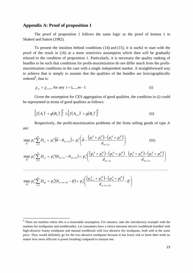
Appendix A: Proof of proposition 1

The proof of proposition 1 follows the same logic as the proof of lemma 1 in

Shaked and Sutton (1982).

To present the intuition behind conditions (14) and (15), it is useful to start with the

proof of the result in (16) at a more restrictive assumption which then will be gradually

relaxed to the condition of proposition 1. Particularly, it is necessary the quality ranking of

bundles to be such that conditions for profit-maximization do not differ much from the profit-

maximization conditions in the case with a single independent market. A straightforward way

to achieve that is simply to assume that the qualities of the bundles are lexicographically

ordered9, that is:

11 iin , for any 1,...,1 mi (i)

Given the assumption for CES aggregation of good qualities, the condition in (i) could

be represented in terms of good qualities as follows:

rrr

ir

r

n

r

i BgAfBgAf1

11

1

(ii)

Respectively, the profit-maximization problems of the firms selling goods of type A

are:

21/1

121

121/11

1

111

maxn

BAB

n

A

A

n

An

j

j

A

p d

ppppppDp

A (iii)

31/2

132

21/1

121

231/221/12

1

222

maxn

BAB

n

A

n

BAB

n

A

A

nn

An

j

j

A

p d

pppp

d

ppppppDp

A

………………………………………………………………………………………………….

1/1

11

1/1

1

maxmnm

BA

m

B

n

A

mA

mmnm

A

m

n

j

mj

A

mp d

ppppppDp

Am

9 There are markets where this is a reasonable assumption. For instance, take the introductory example with the

markets for toothpastes and toothbrushes. Let consumers have a choice between electric toothbrush bundled with

high-abrasive foamy toothpaste and manual toothbrush with low-abrasive dry toothpaste, both sold at the same

price. They would definitely go for the low-abrasive toothpaste because it has lower risk to harm their teeth no

matter how more efficient is power brushing compared to manual one.

24

The corresponding first-order conditions for optimality are given by the following

system of equations:

02

21/1

121

n

BAB

n

A

d

pppp (iv)

022

31/2

132

21/1

121

n

BAB

n

A

n

BAB

n

A

d

pppp

d

pppp

……………………………………………………..

02

1/1

11

mnm

BA

m

B

n

A

m

d

pppp

which after further simplification in the context of Shaked and Sutton (1982) would look as

follows:

21/1

12

21/12n

B

n

BA

nd

ppp (v)

21/1

2

31/2

13

31/221/1 2n

A

n

B

n

BA

nnd

p

d

ppp

………………………………….

11/2

1

1/1

1

1/111/2 2

mnm

A

m

mnm

B

n

BA

m

mnmmnmd

p

d

ppp

1/1

1/1

mnm

A

m

mnmd

p

From (v) the following relation between the marginal taste parameters can be derived:

1/1

1

31/221/1 2...42 mnm

m

nn

(vi)

Since 42 1 m for any 2m , the result in (vi) complies with the inequality in (16).

Note, however, that in order for the inequality in (16) to hold it is not necessary the

qualities of all bundles to be lexicographically ordered. It is sufficient the lexicographical

ordering to hold for just the bundles based on A1 and A2, as required by the following

condition:

211 n and 312 n (vii)

25

As long as A1Bn is better than A2B1 and A2Bn is better than A3B1, the first two

equations of (v) would still hold which means that following part of (vi) is valid:

31/221/1 42 nn (vii)

Next, note that whatever is the bundle quality ranking always the bundle of the best

ranked goods of both types, A1B1, will have the top quality. Also, the best-quality bundles

containing respectively A2 and A3 should always be A2B1 and A3B1.

Respectively, the lowest-quality bundle containing A1 should always be A1Bn while

the worst-quality bundle containing A2 should be respectively A2Bn.

Therefore, due to the expectation all bundles to have demand at unrestricted market,

the following inequality must hold at equilibrium:

'/1'4/331/2 ... mjjmjjn , nj ,...,1 ; nj ,...,1' ; 'jj (viii)

Taken together, conditions (vii) and (viii) imply directly the inequality in (16).

Now, the last stage of the relaxation procedure would be to allow for even the bundles

based on A1 and A2 not to have lexicographically ordered qualities and show that at the

conditions of proposition 1 still the logic behind the result in (16) holds.

Note that for any possible ranking of the bundle qualities, there will always be a set of

more than one bundle based on A1 which are better than A2B1 the best bundle

containing A210

. In proposition 1, the number of the bundles in the set is given by the

parameter k.

Similarly, for any possible ranking of the bundles by quality, there will always be a set

of more than one bundle based on A2 which are better than the higher ranked between

A3B1 - the best bundle containing A3, and A1Bk+1 - the best of the bundles based on A1

which are worse than A2B1. In proposition 1, the number of the bundles in the set is given by

the parameter l.

The corresponding ranking of the top lk bundles is given by the following

expression:

11312222111211 ,...... klk Max (ix)

Note that as long as only the best k bundles based on A1 are sold, the first-order

optimality condition for profit maximization of A1 would not change much, just n in the

indices of the first equation of (v) will be replaced by k:

10

One might argue that even A1B2 could be worse than A2B1. However, note that in that case A and B will just

change their roles in defining bundles’ qualities. So, again there will be a set of more than one bundle this time

based on B1 which are better than A1B2, the best bundle based on B2.

26

0221/1

12

21/1

1

1

1

1

1

1

k

B

k

BA

kA

k

j

j

Ak

j

jd

ppp

p

D

pD (x)

Similarly, as long as only the best l bundles based on A2 are sold, n in the indices of

the second equation of (v) will be replaced by l.

1131

11/2

11

11/221/1

2

2

1

2

1

2

1131

31/2

13

31/221/1

2

2

2

2

1

2

given ,02

given ,02

k

kl

B

l

B

k

A

klkA

l

j

j

Al

j

j

k

l

B

l

BA

lkA

l

j

j

Al

j

j

d

ppp

p

D

pD

d

ppp

p

D

pD

(xi)

In the expressions above, demands and prices are asterisked to distinguish them from the case

when all bundles based on A1 and A2 are sold.

Note also that after simplification both (x) and (xi) imply that the price elasticity of

demand (labeled below by lkII ,, ) must be unit at equilibrium:

11

1

1

1

1

1

A

k

j

j

k

j

j

A

kp

D

D

p (xii)

12

1

2

1

2

2

A

l

j

j

l

j

j

A

lp

D

D

p (xiii)

Now, let’s consider how the first-order optimality conditions change when all n

bundles based on A1 and A2 are sold. The sum of the demands for the bundles that are not

among the best k, respectively l, needs to be added to the profit functions of A1 and A2. Since

its first derivative gives the right-hand side of (x) and (xi), these equations now should change

as follows:

01

1

1

1

1

1

1

1

1

1

1

A

n

kj

j

A

k

j

j

An

kj

j

k

j

jp

D

p

D

pDD (xiv)

27

01

1

2

1

1

2

2

1

2

1

2

A

n

kj

j

A

l

j

j

An

lj

j

l

j

jp

D

p

D

pDD (xv)

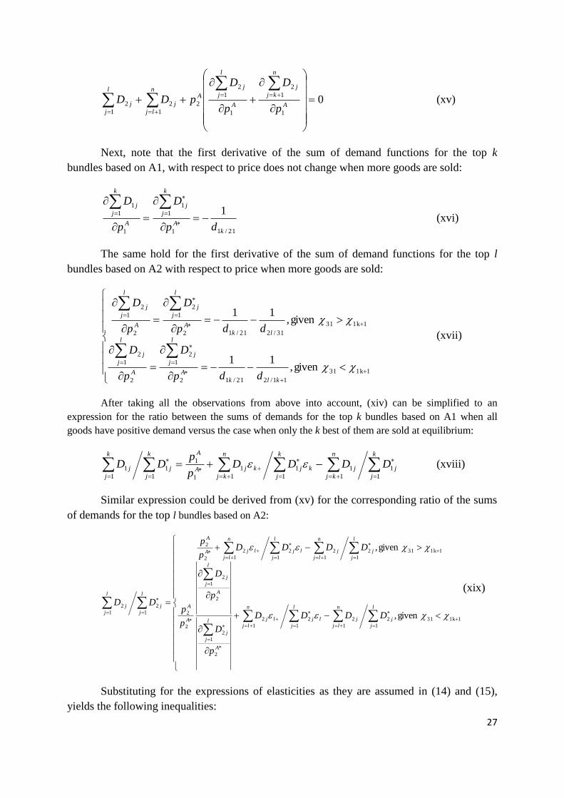
Next, note that the first derivative of the sum of demand functions for the top k

bundles based on A1, with respect to price does not change when more goods are sold:

21/11

1

1

1

1

11

k

A

k

j

j

A

k

j

j

dp

D

p

D

(xvi)

The same hold for the first derivative of the sum of demand functions for the top l

bundles based on A2 with respect to price when more goods are sold:

11k31

11/221/12

1

2

2

1

2

11k31

31/221/12

1

2

2

1

2

given ,11

given ,11

klk

A

l

j

j

A

l

j

j

lk

A

l

j

j

A

l

j

j

ddp

D

p

D

ddp

D

p

D

(xvii)

After taking all the observations from above into account, (xiv) can be simplified to an

expression for the ratio between the sums of demands for the top k bundles based on A1 when all

goods have positive demand versus the case when only the k best of them are sold at equilibrium:

k

j

j

n

kj

jk

k

j

jk

n

kj

jA

Ak

j

j

k

j

j DDDDp

pDD

1

1

1

1

1

1

1

1

1

1

1

1

1

1 (xviii)

Similar expression could be derived from (xv) for the corresponding ratio of the sums

of demands for the top l bundles based on A2:

l

j

j

n

lj

jl

l

j

jl

n

lj

j

A

l

j

j

A

l

j

j

A

A

l

j

j

n

lj

jl

l

j

jl

n

lj

jA

A

l

j

j

l

j

j

DDDD

p

D

p

D

p

p

DDDDp

p

DD

1

11k312

1

2

1

2

1

2

*

2

1

2

2

1

2

2

2

1

11k312

1

2

1

2

1

2

2

2

1

2

1

2

given ,

given ,

(xix)

Substituting for the expressions of elasticities as they are assumed in (14) and (15),

yields the following inequalities:

28

111

1

1

1

1

1

1

1

1

1

1

1

1

1

k

j

j

n

kj

j

k

j

j

n

kj

jA

Ak

j

j

k

j

j DDDDp

pDD (xx)

l

j

j

n

lj

j

l

j

j

n

lj

j

A

l

j

j

A

l

j

j

A

A

l

j

j

n

lj

j

l

j

j

n

lj

jA

A

l

j

j

l

j

j

DDDD

p

D

p

D

p

p

DDDDp

p

DD

1

11k312

1

2

1

2

1

2

*

2

1

2

2

1

2

2

2

1

11k312

1

2

1

2

1

2

2

2

1

2

1

2

given ,11

given ,11

(xxi)

After representing the demands in explicit form, the above results look as follows:

21/121/121/121/1 kkkk i.e. 21/12 k (xxii)

11k3111/221/111/2/211/2/211/221/111/221/1

11k3131/221/131/231/231/221/131/221/1

given ,2 i.e.

given , 2 i.e.

klkkllkllklkklk

lklllklk (xxiii)

Combined (xxii) and (xxiii) imply directly the relationship in (16). So, the proof of

proposition 1 is complete.

29

Appendix B: Proof of proposition 2

Proposition 2 can be proven by induction. In what follows, the proof is presented for

the case when the qualities of bundles are assumed to be lexicographically ordered. However,

it is straightforward to show that it also holds for the relaxed assumption of proposition 1.

Let’s introduce a third good hzCz ,...,1, . Given the bundle quality ranking of (i), the

profit-maximization problems of the firms producing goods of type A would look as follows:

211/1

1121

11 nh

CBAC

h

B

n

A

A

p d

pppppppMax

A (xxiv)

311/2

1132

211/1

1121

22 nh

CBAC

h

B

n

A

nh

CBAC

h

B

n

A

A

p d

pppppp

d

pppppppMax

A

……………………………………………………………………………….

11/1

111

111/2

1112

11 mnhm

CBA

m

C

h

B

n

A

m

mnhm

CBA

m

C

h

B

n

A

mA

mp d

pppppp

d

pppppppMax

Am

Omnh

Omnh

C

h

B

n

A

m

mnhm

CBA

m

C

h

B

n

A

mA

mp

Omnh

mnhm

CBA

m

C

h

B

n

A

mA

mp

d

ppp

d

pppppppMax

d

pppppppMax

Am

Am

/

/11/1

111

/

11/1

111

if ,

if ,

Respectively, the first-order optimality conditions are given by the system of

equations (xxv) below:

211/1

112

211/12nh

C

h

B

n

CBA

nhd

ppppp (xxv)

211/1

2

311/2

113

311/2211/1 2nh

A

nh

C

h

B

n

CBA

nhnhd

p

d

ppppp

……………………………………………………………..

111/2

1

11/1

11

11/1111/2 2

mnhm

A

m

mnhm

C

h

B

n

CBA

m

mnhmmnhmd

p

d

ppppp

Hence, the following expression for the relation between the corresponding taste

parameters could be derived:

11/1

1

311/2211/1 2...42 mnhm

m

nhnh

(xxvi)

30

Note that the same condition which is sufficient

4

for at most two goods to

have positive demand at equilibrium in a single-good market, allows for up to n2 bundles

to be sold in a market for two-good bundles and for up to hn2 bundles in a market for

three-good bundles - 1,for ,222 hnnhn . As the number of goods in a bundle

rises, the number of bundles in which a good could take part is also increasing. This implies a

more restrictive condition on the range of consumer tastes to hold for ensuring positive

market share of at most 2 bundles.

Given that at most A1 and A2 could be sold in equilibrium, the profit-maximization

problems of the firms selling goods of type B in three-good market would look as follows:

221/21

121

211/1

121

121/11

121

11 h

CBC

h

B

nh

C

h

BAC

h

B

n

A

h

CBC

h

B

B

p d

pppp

d

pppppp

d

pppppMax

B (xxvii)

131/12

13121

121/11

12111

22 h

CBAC

h

BA

h

CBAC

h

BA

B

p d

pppppp

d

pppppppMax

B

231/22

13222

221/21

12212

h

CBAC

h

BA

h

CBAC

h

BA

d

pppppp

d

pppppp

………………………………………………………………………………………………

12/12

11

112/22

112

11/11

11

111/21

112

11 nhn

CB

n

B

h

A

n

nhn

CB

n

B

h

A

n

nhn

CB

n

B

h

A

n

nhn

CB

n

B

h

A

nB

np d

pppp

d

pppp

d

pppp

d

pppppMax

Bn

311/2

1132

12/12

11

211/1

11

11/11

11

nh

CBAC

h

B

n

A

nhn

CB

n

C

h

B

n

nh

CBC

h

B

n

nhn

CB

n

C

h

B

nB

np d

pppppp

d

pppp

d

pppp

d

pppppMax

Bn

The corresponding system of the first-order optimality conditions looks as follows:

211/1

1

221/21121/11

12221/21121/11211/1

1122

nh

B

hh

C

h

CB

hhnhd

p

ddppp

(xxviii)

221/21121/11

2

231/22131/12

13231/22131/12221/21121/11

111122

hh

B

hh

C

h

CB

hhhhdd

pdd

ppp

………………………………………………………………………………………………..

112/22111/21

1

12/1211/11

112/1211/11112/22111/21

111122

nhnnhn

B

n

nhnnhn

C

h

CB

nnhnnhnnhnnhndd

pdd

ppp

31

The optimality results in (xxvi) and (xxviii) imply the following relationship between

taste parameters:

12/12

1

11/11

1

231/22131/12221/21121/11 22...44222

3nhn

n

nhn

n

hhhh

(xxix)

Apparently, even the condition

8

3 which in a market for two-good bundles is

sufficient for at most two bundles to have positive demand in equilibrium allows for up to

h2 bundles to be sold in a market for three-good bundles. Therefore, for at most two

bundles to be demanded at the equilibrium prices, stronger restriction is required as shown in

the analysis of profit-maximization of the firms offering goods of type C. Their respective

optimization problems look as follows:

122/121

21

121/11

122

112/111

211

1 d

pp

d

pppp

d

pppMax

CC

h

CBC

h

BCCC

pC (xxx)

123/122

32

122/121

21

113/112

32

112/111

212

2 d

pp

d

pp

d

pp

d

pppMax

CCCCCCCCC

pC

…………………………………………………………………..

hh

C

h

C

h

hh

C

h

C

h

hh

C

h

C

h

hh

C

h

C

hC

hp d

pp

d

pp

d

pp

d

pppMax

Ch 12/112

1

112/212

12

11/111

1

111/211

12

11

hh

CBC

h

B

hh

C

h

C

h

h

CBC

h

B

hh

C

h

C

hC

hp d

pppp

d

pp

d

pppp

d

pppMax

Ch 12/112

132

12/112

1

121/11

121

11/111

1

The first-order optimality conditions could be represented by the following system of

equations:

121/11

1

122/121112/111

2122/121112/111121/11

1122

h

CC

hd

p

ddp

(xxxi)

122/121112/111

2

123/122113/112

3123/122113/112122/121112/111

111122

ddp

ddp CC

…………………………………………………………………………………………..

112/212111/211

1

12/11211/111

12/11211/111112/212111/211

111122

hhhh

C

h

hhhh

C

hhhhhhhhhdd

pdd

p

32

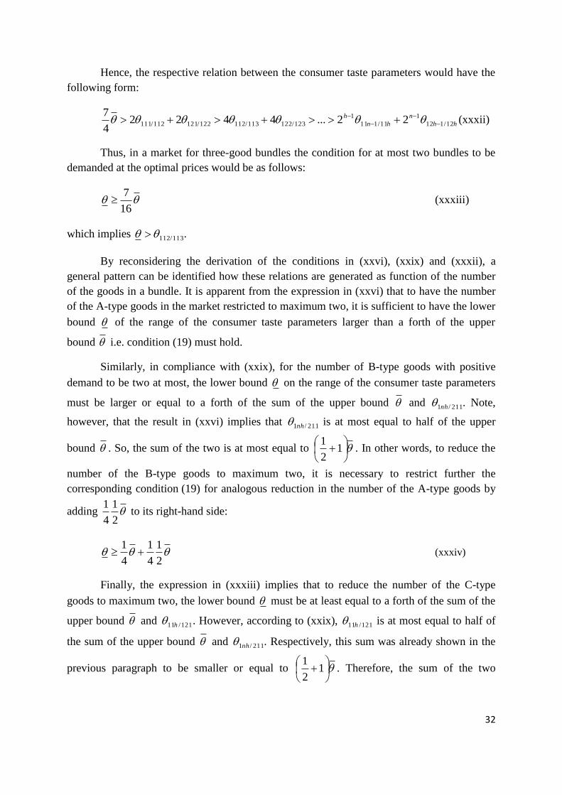
Hence, the respective relation between the consumer taste parameters would have the

following form:

hh

n

hn

h

12/112

1

11/111

1

123/122113/112122/121112/111 22...44224

7

(xxxii)

Thus, in a market for three-good bundles the condition for at most two bundles to be

demanded at the optimal prices would be as follows:

16

7 (xxxiii)

which implies 113/112 .

By reconsidering the derivation of the conditions in (xxvi), (xxix) and (xxxii), a

general pattern can be identified how these relations are generated as function of the number

of the goods in a bundle. It is apparent from the expression in (xxvi) that to have the number

of the A-type goods in the market restricted to maximum two, it is sufficient to have the lower

bound of the range of the consumer taste parameters larger than a forth of the upper

bound i.e. condition (19) must hold.

Similarly, in compliance with (xxix), for the number of B-type goods with positive

demand to be two at most, the lower bound on the range of the consumer taste parameters

must be larger or equal to a forth of the sum of the upper bound and 211/1nh . Note,

however, that the result in (xxvi) implies that 211/1nh is at most equal to half of the upper

bound . So, the sum of the two is at most equal to

1

2

1. In other words, to reduce the

number of the B-type goods to maximum two, it is necessary to restrict further the

corresponding condition (19) for analogous reduction in the number of the A-type goods by

adding 2

1

4

1 to its right-hand side:

2

1

4

1

4

1 (xxxiv)

Finally, the expression in (xxxiii) implies that to reduce the number of the C-type

goods to maximum two, the lower bound must be at least equal to a forth of the sum of the

upper bound and 121/11h . However, according to (xxix), 121/11h is at most equal to half of

the sum of the upper bound and 211/1nh . Respectively, this sum was already shown in the

previous paragraph to be smaller or equal to

1

2

1. Therefore, the sum of the two

33

parameters and 121/11h cannot be larger than

1

2

1

2

11 . In other words, to reduce

the number of the C-type goods to maximum two, it is necessary to restrict further the

condition in (xxxiv) for analogous reduction in the number of the B-type goods by adding

1

2

1

2

1

4

1 to its right-hand side:

1

2

1

2

1

4

1

2

1

4

1

4

1 (xxxv)

From the comparison of (19), (xxxiv) and (xxxv) it is trivial that each additional unit

added to the number of goods in a bundle increases by half the restriction from below on the

lower bound for at most two bundles to be sold at the equilibrium prices. Hence, the

general form of this condition would look as shown below:

X

xx

X

x

x

11

1

1

2

1

2

1

4

1 (xxxvi)

which completes the proof of proposition 2 for the case when assumption (i) holds.

34

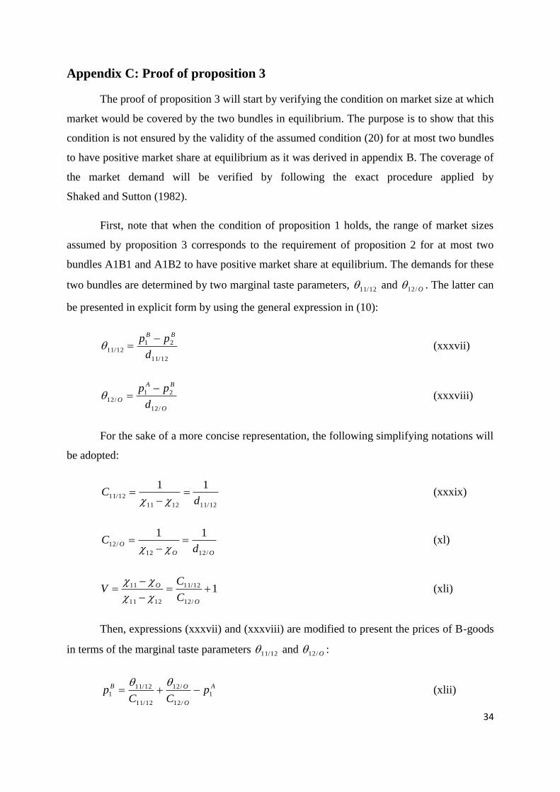
Appendix C: Proof of proposition 3

The proof of proposition 3 will start by verifying the condition on market size at which

market would be covered by the two bundles in equilibrium. The purpose is to show that this

condition is not ensured by the validity of the assumed condition (20) for at most two bundles

to have positive market share at equilibrium as it was derived in appendix B. The coverage of

the market demand will be verified by following the exact procedure applied by

Shaked and Sutton (1982).

First, note that when the condition of proposition 1 holds, the range of market sizes

assumed by proposition 3 corresponds to the requirement of proposition 2 for at most two

bundles A1B1 and A1B2 to have positive market share at equilibrium. The demands for these

two bundles are determined by two marginal taste parameters, 12/11 and O/12 . The latter can

be presented in explicit form by using the general expression in (10):

12/11

2112/11

d

pp BB (xxxvii)

O

BA

Od

pp

/12

21/12

(xxxviii)

For the sake of a more concise representation, the following simplifying notations will

be adopted:

12/111211

12/11

11

dC

(xxxix)

OO

Od

C/1212

/12

11

(xl)

1/12

12/11

1211

11

O

O

C

CV

(xli)

Then, expressions (xxxvii) and (xxxviii) are modified to present the prices of B-goods

in terms of the marginal taste parameters 12/11 and O/12 :

A

O

OB pCC

p 1

/12

/12

12/11

12/11

1

(xlii)

35

A

O

OB pC

p 1

/12

/12

2

(xliii)

Now, expressions (xxxix) and (xl) could be substituted for the prices of B-goods in the

optimality conditions for profit-maximization to derive 12/11 as a best response to O/12 :

2

1 12/111/12

12/11

CpV A

O

(xliv)

12/111/1212/11 1 CpV A

O , if market is covered i.e. O/12 (xliv)

O

A

O CCpV /1212/111/1212/11 1 , if market is not covered i.e. O/12 (xlvi)

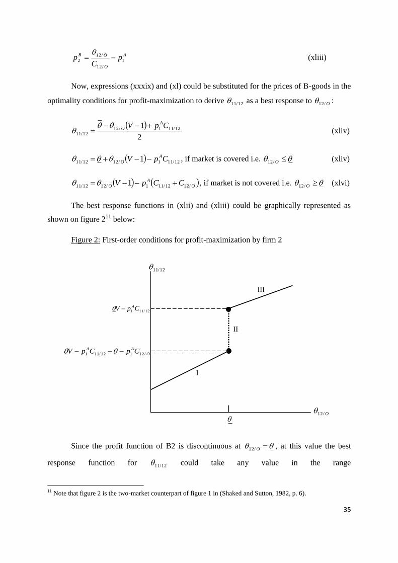
The best response functions in (xlii) and (xliii) could be graphically represented as

shown on figure 211

below:

Figure 2: First-order conditions for profit-maximization by firm 2

Since the profit function of B2 is discontinuous at O/12 , at this value the best

response function for 12/11 could take any value in the range

11

Note that figure 2 is the two-market counterpart of figure 1 in (Shaked and Sutton, 1982, p. 6).

12/11

O/12

III

II

I

12/111 CpV A

O

AA CpCpV /12112/111

36

12/111/1212/111 ,)1( CpVCCpV A

O

A . Respectively, three segments of its graph could

be distinguished on figure 2. Whether the optimal solution of the B-good profit maximization

lies in segment I, II or III depends on where the vertical O/12 is cut by the strictly

decreasing best-response function of (xliv):

3

3

3

233

3

3

3

233

if IIIsegment

if IIsegment

if Isegment

12/111

/1212/11112/111

/1212/111

CpV

CCpV

Cp

CCpV

A

O

AA

O

A

As in Shaked and Sutton (1982), the expression in (xli) implies that V is larger than 1.

Hence, the solution cannot be in segment III, as long as the right-hand side of the respective

inequality above is at most 1 which after simplification corresponds to the following condition

on the market size:

2

Apparently, distinct from Shaked and Sutton (1982), the above condition is not

ensured by the restriction on market size which is imposed by (20) for at most two bundles to

have positive market shares at equilibrium. Therefore, it is possible in the range of the market

size

28

3

assumed by proposition 3, the market not to be covered at equilibrium.

In what follows, the solution of the profit-maximization problem will be consecutively

derived for covered and non-covered market, respectively. The solution for the pricing

subgame equilibrium will be given by comparison between the two results.

The profit-maximization problems of the three firms in the case of covered market

(denoted by adding c in the upper index) would look as follows:

AcA

ppMax

A 1

_

11

(xlvii)

37

12/11

21112/111

_

11 d

ppppMax

BBBBcB

pB

12/11

21212/112

_

22 d

ppppMax

BBBBcB

pB

To derive the optimal prices for B1 and B2, it is enough to consider just the last two

problems whose solution is given by the following system of first-order optimality conditions:

02 12/1121 dpp BB (xlviii)

02 12/1121 dpp BB

The respective solution for the prices is as follows:

12/11

_

1 23

1dp cB (xlix)

12/11

_

2 23

1dp cB

The optimal price of good A1 is given as a corner solution at which the market is

covered:

121112/1112212

_

1 23

12

3

1 dpp BcA (l)

Now, the equilibrium marginal taste parameter 12/11 could be derived as follows:

312/11

_

2

_

112/11

d

pp cBcB

(li)

which implies that for at least the two bundles A1B1 and A1B2 to have positive market share,

the following condition must hold:

03

212/11

i.e.

2

(lii)

So, in the market size range assumed by proposition 3, B2 has a chance to make

positive sales as long as A1 is charged a price at which the market would be covered.

In case of non-covered market (denoted by adding nc in the upper index), the respective

profit-maximization problems for the three firms would look as follows:

38

O

BAA

O

AncA

p d

ppppMax

A

/12

211/121

_

11

(liv)

12/11

21112/111

_

11 d

ppppMax

BBBBncB

pB

O

BABBB

O

BncB

p d

pp

d

ppppMax

B

/12

21

12/11

212/1212/112

_

22

The optimal prices are given by the solution of the following system of first-order

optimality conditions:

02 /1221 O

BA dpp (lv)

02 12/1121 dpp BB

02 12/11/122/12112/111 ddpdpdp O

B

O

BA

The respective solution for the prices is as follows:

2

/12_

1

OncA dp

(lvi)

2

12/11_

1

dp ncB

0_

2 ncBp

Note, however, that in this case even pricing at zero would not ensure positive demand

for B2 at equilibrium because the optimal response of A1 and B1 would drive it out from the

market. To show that, substitute (lvi) for the prices in the expressions for the marginal taste

parameters 12/11 and O/12 :

2/1212/11

O

Hence, the respective demand for B2 is zero, as shown below:

0/1212/1112 OD (lvii)

So, for B2 there will not be an incentive to enter if A1 is going to set price at which

the market would not be covered. Given no entry decision by B2, the profit maximization

problems (denoted by adding m for ‘monopoly’ in the upper index) of A1 and B1 as only

entrants in the first stage would look as follows:

39

O

BAA

O

AncmA

p d

ppppMax

A

/11

111/111

_

11

(lviii)

O

BAB

O

BncmB

p d

ppppMax

B

/11

111/111

_

11

which implies that both entrants will charge the same prices as shown below:

3

/11_

1

OncmA dp

(lix)

3

/11_

1

OncmB dp

Substituting for the prices from (lix) in the expression for the marginal taste parameter

O/11 yields the following result:

3

2/11

O (lx)

That is, at equilibrium the market would not be covered as long as 3

2

2

.

Finally, it remains only to compare the optimal profits of A1 which drive its decision

to set a price at which the market is covered or not after B2 enters the market in the first stage.

If B2 is in the market and A1 chooses to set a price at which the market would be

covered, its optimal profit is given by substituting for the prices from (l) in its profit function:

12/11/12

_

13

2dd O

cA (lxi)

Alternatively, if A1 chooses to set a price at which the market would not be covered,

its optimal profit is given by substituting for the prices from (lvi) in its profit function:

4

/12

2

_

1

OncA d (lxii)

40

Subtracting (lxi) from (lxii) yields the following expression:

12/11/12

_

1

_

1 423212

1dd O

cAncA (lxiii)

which is strictly positive for 2

1 . That is, given entry by B2, the entrant offering good A1

would be strictly better-off from charging price 2

/12

1

OA dp

at which the sales of B2 would

be foreclosed and the market would not be covered.

The last result implies that entry-deterrence threat would be credible for the assumed

range of market sizes in proposition 3. So, B2 will stay out of the market and only A1 and B1

will enter at equilibrium. Furthermore, in compliance with the result in (lx), the market will

not be covered. This completes the proof of proposition 3.

41

Appendix D: Quality-choice subgame equilibrium

Substituting for the prices from (lix) in the profit functions of the firms entering with

goods A1 and B1, respectively, allows to derive the equilibrium profits in terms of quality

difference Od /11 :

9

/11

2

11

OBA d (lxiv)

Substituting for the explicit expression of Od /11 :

Or

rr

OO uBgAfud 1

1111/11

from (8) and (13) yields the following expressions for the profits in terms of product qualities:

9

1

11

2

11

Or

rr

BA

uBgAf

(lxv)

Obviously, (lxv) is strictly increasing in both 1Af and 1Bg which implies that

profit-maximizing quality choice for both A1 and B1 is given by the corner solution where

they are assigned the upper bounds of their quality intervals:

FAf 1 (lxvi)

GBg 1

This completes the solution for the subgame equilibrium in the quality-choice stage.