vertical motion observed with gps: what can we learn...

1
Vertical motion observed with GPS: What can we learn about regional geophysical signals, Earth structure, and rheology? H.-P. Plag * , W. Hammond, C. Kreemer, G. Blewitt Nevada Bureau for Mines and Geology and Seismological Laboratory University of Nevada, Reno, Mail Stop 178, Reno, NV 89557, * email: [email protected] Introduction Tectonic studies utilizing observations of surface displacements from GPS are based predominantly on observations of hor- izontal displacements, while vertical displacements mostly provide constraints for loading-related geophysical processes. A main reason for this disjunct use of GPS observations is that tectonic signals often are larger in the horizontal component while loading signals dominantly are contained in the vertical component. Moreover, the horizontal components of GPS-determined displacements have a precision about three times that of the vertical component. Considering the growing number of PBO stations with records potentially long enough to determine reliable secular trends, it is worthwhile to ask the question to what extent vertical displacement time series can be used to constrain tectonic processes, Earth structure, and rheology. In order to answer this question, we study the anatomy of time series of vertical displacements determined from regional and local GPS networks in North America and derive the spatio-temporal pattern of vertical crustal motion as seen by these networks. 15 30 45 60 75 15 30 45 60 75 195 210 225 240 255 270 285 300 315 195 210 225 240 255 270 285 300 315 15 30 45 60 75 15 30 45 60 75 195 210 225 240 255 270 285 300 315 195 210 225 240 255 270 285 300 315 15 30 45 60 75 15 30 45 60 75 195 210 225 240 255 270 285 300 315 195 210 225 240 255 270 285 300 315 15 30 45 60 75 15 30 45 60 75 195 210 225 240 255 270 285 300 315 195 210 225 240 255 270 285 300 315 15 30 45 60 75 15 30 45 60 75 195 210 225 240 255 270 285 300 315 195 210 225 240 255 270 285 300 315 30 35 40 45 50 30 35 40 45 50 235 240 245 250 255 260 235 240 245 250 255 260 30 35 40 45 50 30 35 40 45 50 235 240 245 250 255 260 235 240 245 250 255 260 30 35 40 45 50 30 35 40 45 50 235 240 245 250 255 260 235 240 245 250 255 260 30 35 40 45 50 30 35 40 45 50 235 240 245 250 255 260 235 240 245 250 255 260 30 35 40 45 50 30 35 40 45 50 235 240 245 250 255 260 235 240 245 250 255 260 Figure 1: GPS stations used in the present anal- ysis. Upper diagram: North America. Lower diagram: GPS station distribution in the West- ern U.S.A. The Data We have collected GPS observations for North American stations from the publicly available archives at UNAVCO, SOPAC, and CORS as well as our own MAGNET archive (Figure 1). The focus of our studies is the South- Western part of the U.S., and there station distribution is densest (Figure 2). All the GPS data were homogenously processed with the GIPSY-OASIS II (GIPSY) software package of Jet Propulsion Laboratory (JPL) using the Precise Point Positioning (PPP) method (Zumberge et al., 1997) to determine daily coordinates, with ambiguity resolution applied across the entire network by automatic selection of the ionospheric- or pseudorange- widelane method (Blewitt, 1989). Satellite orbit and clock parameters were provided by JPL. Ionosphere-free combinations of carrier phase and pseudorange were processed every 5 minutes. To account for atmosphere effects that can bias the inference of the antenna phase center height we solve simultaneously for station height, zenith path delay and tropospheric gradient parameters. We processed the data with a satellite elevation cut- off angle of 15 in order to minimize the effects of atmospheric refraction and multipath. Compared to lower cutoff elevations, this results, on the one hand, in less data used and hence more uncertainty in individual daily positions, and, on the other hand, in lower bias of station coordinates as- sociated with atmospheric refraction of the GPS signal, which is greatest for satellites at low elevation. Ambiguity resolution was carried out on the complete North American network. All time series were determined in ITRF2000. Time series of daily station displacements are computed with respect to the coordinates at epoch 2000/02/01. No spatial filtering has been applied to the time series. These time series were then used to determine vertical rates taking into account semi-annual and annual harmonic constituents. For time series analysis, the time window from 2000/02/01 to 2006/10/31 was used in order to avoid offsets due to the transition of JPL from ITRF2000 to ITRF2005. Time series Figure 2 shows time series of vertical displacements for selected North American stations. Day-to-day variation and intrasea- sonal to interannual variations are of the order of ±20 mm and ±10 mm, respectively. Most station exhibit a linear trend, and a seasonal cycle is discernible. For stations separated on the order of 10 3 km, considerable differences in the intrasea- sonal and interannual variations are visible (see Figure 2, left diagrams). On local scale (up to 500 km, see the example of the Basin and Range Province, Figure 2), the differences on intra- to interannual time scales are very small, while the main difference are in the day-to-day variations (Figure 2, right diagrams). The displacement time series are a combination of geophysical signals and apparent displacements induced by the GPS system and data analysis. Concerning the observed interannual variations, a key problem is the separation of instrumental and analysis effects from the geophysical signals. The interannual variations have surprisingly small spatial scales, of the order of 10 3 km (see below), with significant spatial variations over North America. If these variations were solely due to GPS-system and analysis effects, we would expect larger spatial scales in these variations. Spectrum The discrete part of the spectrum of the daily displacement time series is generally dominated by a semi-annual and annual harmonic constituent, denoted here as Sa and Ssa, respectively (Figure 3). The ratio of the amplitudes of Sa and Ssa changes from station to station. Cross-correlation The cross-correlation coefficient for the vertical displacement time series (station pairs) varies considerably between ±0.8 even for nearby stations. (Figure 4, left diagram). No clear spatial pattern is discernible. However, if linear trend and annual and semi-annual constituents are removed, cross-correlation for the residual time series increases considerably (Figure 4, right diagram). Taking individual stations as base, even for distances of order 10 3 km, correlation coefficients are generally between 0.6 and 0.8 (Figure 5). For distances larger than order 10 3 km, the cross-correlation decreases and breaks down for distances larger than 2 · 10 3 km. This latter feature is somewhat uncertain due to the sparse number of station pairs with great distances. PIE1 2000.00 2001.60 2003.20 2004.80 2006.40 Year -50 0 50 100 mm FRED -50 0 50 100 mm NAIU -50 0 50 100 mm STJO -50 0 50 100 mm CHUR -50 0 50 100 mm WHIT -50 0 50 100 mm YELL -50 0 50 100 mm Up PIE1 2000.00 2001.60 2003.20 2004.80 2006.40 Year -50 0 50 100 mm FRED -50 0 50 100 mm NAIU -50 0 50 100 mm STJO -50 0 50 100 mm CHUR -50 0 50 100 mm WHIT -50 0 50 100 mm YELL -50 0 50 100 mm Up FERN 2000.00 2001.60 2003.20 2004.80 2006.40 Year -45 -15 15 45 mm SHOS -45 -15 15 45 mm APEX -45 -15 15 45 mm FRED -45 -15 15 45 mm ALAM -45 -15 15 45 mm ECHO -45 -15 15 45 mm RAIL -45 -15 15 45 mm Up FERN 2000.00 2001.60 2003.20 2004.80 2006.40 Year -45 -15 15 45 mm SHOS -45 -15 15 45 mm APEX -45 -15 15 45 mm FRED -45 -15 15 45 mm ALAM -45 -15 15 45 mm ECHO -45 -15 15 45 mm RAIL -45 -15 15 45 mm Up Figure 2: Time series of vertical displacements. Left two diagrams: Stations distributed from 31 to 65 N. Right two diagrams: Stations in the Basin and Range Province. In each pair, the time series of vertical displacements are shown in the left diagram, while the right diagram shows for each station the difference to the time series at the bottom. The offset around Nov. 5, 2006 is due to the transition of JPL to ITRF2005. V 0 2 4 6 8 10 Frequency cpy 0.00 1.80 3.60 5.40 7.20 9.00 Variance % A 0.00 1.40 2.80 4.20 5.60 7.00 Amplitude mm V 0 2 4 6 8 10 Frequency cpy 0 4 8 12 16 20 Variance % A 0.00 1.60 3.20 4.80 6.40 8.00 Amplitude mm V 0 2 4 6 8 10 Frequency cpy 0 4 8 12 16 20 Variance % A 0 4 8 12 16 20 Amplitude mm V 0 2 4 6 8 10 Frequency cpy 0.00 1.60 3.20 4.80 6.40 8.00 Variance % A 0.00 0.80 1.60 2.40 3.20 4.00 Amplitude mm V 0 2 4 6 8 10 Frequency cpy 0 6 12 18 24 30 Variance % A 0.00 1.60 3.20 4.80 6.40 8.00 Amplitude mm V 0 2 4 6 8 10 Frequency cpy 0 4 8 12 16 20 Variance % A 0.00 1.40 2.80 4.20 5.60 7.00 Amplitude mm V 0 2 4 6 8 10 Frequency cpy 0 4 8 12 16 20 Variance % A 0.00 1.40 2.80 4.20 5.60 7.00 Amplitude mm Figure 3: Spectrum of se- lected time series. Stations are from top left to bottom right: YELL, WHIT, CHUR, STJO, NAIU, FRED, PIE1. 0 20 40 60 80 100 120 140 160 180 200 0 20 40 60 80 100 120 140 160 180 200 0 20 40 60 80 100 120 140 160 180 200 0 20 40 60 80 100 120 140 160 180 200 -0.2 0.1 0.4 0.7 1.0 Correlation 0 20 40 60 80 100 120 140 160 180 200 0 20 40 60 80 100 120 140 160 180 200 0 20 40 60 80 100 120 140 160 180 200 0 20 40 60 80 100 120 140 160 180 200 -0.2 0.1 0.4 0.7 1.0 Correlation Figure 4: Cross-correlation of time series of vertical displace- ments. Stations are approximately order from northwest to southeast. Left: Correlation of original time series. Right: Correlation of residual time series after trend and seasonal cycle have been removed. Sa 30 40 50 60 70 Latitude 0 4 8 12 Amplitude mm Sa 30 40 50 60 70 Latitude 0 120 240 360 Phase deg Ssa 0 4 8 12 Amplitude mm Ssa 0 120 240 360 Phase deg Figure 8: Ampli- tude and phase of Sa and Ssa as function of latitude. Only stations west of 248 are shown. Ori. 0 1200 2400 3600 Station distance km -1.00 -0.60 -0.20 0.20 0.60 1.00 Res. -1.00 -0.60 -0.20 0.20 0.60 1.00 Ori. 0 1200 2400 3600 Station distance km -1.00 -0.60 -0.20 0.20 0.60 1.00 Res. -1.00 -0.60 -0.20 0.20 0.60 1.00 Ori. 0 1200 2400 3600 Station distance km -1.00 -0.60 -0.20 0.20 0.60 1.00 Res. -1.00 -0.60 -0.20 0.20 0.60 1.00 Ori. 0 1200 2400 3600 Station distance km -1.00 -0.60 -0.20 0.20 0.60 1.00 Res. -1.00 -0.60 -0.20 0.20 0.60 1.00 Figure 5: Interstation correlation. Correlation coefficients for station pairs are shown as function of station distance. Base stations are (from top left to bottom right): PIE1, FRED, NAIU, WHIT. Secular Trends. Generally, at interannual periods, the GPS time series of vertical motion show significant nonlinear components potentially contaminating the derived secular velocity field (see Figure 2). Determining reliable secular trends for time series with variations at interannual to decadal and longer time scales requires time series longer than these scale. This is well known from studies of climatological and oceanographic time series, where often 20 to 50 years are considered the minimum record length for trend estimation. However, in the case of climate and oceanography, the signals are mainly due to the Earth system processes, which can be modeled to a large extent. For vertical GPS time series, a significant portion may come from the observing system and data analysis, thus complicating the situation considerably. Nevertheless, the spatial pattern of the secular vertical velocity field displays features potentially related to geophysical processes, including tectonics (Figure 6). In particular, the Basin and Range Province shows mainly significant uplift, which is contrary to the expectation of an extensional basin driven by gravitational potential energy. 30 35 40 45 50 30 35 40 45 50 235 240 245 250 255 260 235 240 245 250 255 260 -4 -2 0 2 4 mm/yr 30 35 40 45 50 30 35 40 45 50 235 240 245 250 255 260 235 240 245 250 255 260 34 35 36 37 38 39 40 41 42 34 35 36 37 38 39 40 41 42 239 240 241 242 243 244 245 246 247 248 239 240 241 242 243 244 245 246 247 248 -4 -2 0 2 4 mm/yr 34 35 36 37 38 39 40 41 42 34 35 36 37 38 39 40 41 42 239 240 241 242 243 244 245 246 247 248 239 240 241 242 243 244 245 246 247 248 Figure 6: Vertical rates in the Western U.S. Left: Western U.S., right: Basin and Range Province. 30 35 40 45 50 30 35 40 45 50 235 240 245 250 255 260 235 240 245 250 255 260 30 35 40 45 50 30 35 40 45 50 235 240 245 250 255 260 235 240 245 250 255 260 30 35 40 45 50 30 35 40 45 50 235 240 245 250 255 260 235 240 245 250 255 260 30 35 40 45 50 30 35 40 45 50 235 240 245 250 255 260 235 240 245 250 255 260 34 35 36 37 38 39 40 41 42 34 35 36 37 38 39 40 41 42 239 240 241 242 243 244 245 246 247 248 239 240 241 242 243 244 245 246 247 248 34 35 36 37 38 39 40 41 42 34 35 36 37 38 39 40 41 42 239 240 241 242 243 244 245 246 247 248 239 240 241 242 243 244 245 246 247 248 34 35 36 37 38 39 40 41 42 34 35 36 37 38 39 40 41 42 239 240 241 242 243 244 245 246 247 248 239 240 241 242 243 244 245 246 247 248 34 35 36 37 38 39 40 41 42 34 35 36 37 38 39 40 41 42 239 240 241 242 243 244 245 246 247 248 239 240 241 242 243 244 245 246 247 248 Figure 7: Seasonal cycle in vertical displacements. Left: Western U.S., right: Basin and Range Province. Top: Annual harmonic constituent. Bot- tom Semi-annual consitituent. Seasonal Cycle Sa and Ssa show high spatial coherency in amplitude and phase over large geographical areas except for few deviations which most likely are due to local influences (Figure 7). The spatial coherency underlines that GPS picks up geophysical signals at the seasonal time scale. The amplitudes of Sa increases from South to North up to latitude 50 N and is smaller again at high latitudes (Figure 8). For Ssa, a general degrease of the amplitude from South to North is found. The spatial pattern of Sa and Ssa as seen by GPS can be used to identify the forcing geophysical signals (loading) and separate these from potential system-induced contribution. Conclusions Beside spatially homogeneous annual and semi-annual harmonic constituents the GPS vertical displacement time series have significant interannual variations with spatial scales of a few hundred to a thousand kilometer, potentially biasing the secular trends determined from time series of a few years to decades. Strictly speaking, if we do not understand the interannual variations of GPS vertical time series, we cannot safely interpret the secular signal in terms of global and regional processes. Spatial filtering, which has been successfully applied to extract the secular signal from horizontal components (Wdowinski et al., 2004, e.g.) does not help to eliminate the interannual signals in the vertical. Part of these variations are due to reference frame instability. Therefore, improving the reference frame seems to be a prerequisite for the interpretation of vertical motion in terms of large-scale tectonic process and must have highest priority. A significant improvement is expected by modeling load-induced deformations in the reference frame determination. The geophysical loading models can be validated against the spatial patterns of Sa and Ssa as seen by GPS. References Blewitt, G., 1989. Carrier phase ambiguity resolution for the Global Positioning System applied to geodetic baselines up to 2000 km, J. Geophys. Res., 94(B8), 10187–10283. Wdowinski,S., Bock, Y., Baer, G., Prawirodirdjo, L., Bechor, N., Naaman, S., Knafo, R., Forrai, Y., & Melzer, Y., 2004. GPS measurements of current crustal movements along the Dead Sea Fault, J. Geophys. Res., 109, (B05403), 1–16. Zumberge, J. F., Heflin, M. B., Jefferson, D. C., & Watkins, M. M., 1997. Precise point positioningfor the efficient and robust analysis of GPS data from large networks, J. Geophys. Res., 102, 5005–5017. Acknowledgments: This work has been conducted with support from NASA Solid Earth and Natural Hazards, NASA Interdisciplinary Science, and by DOE contract FC-08-98NV12081.

Upload: tranque

Post on 07-Apr-2018

216 views

Category:

Documents


2 download

TRANSCRIPT

Vertical motion observed with GPS:What can we learn about regional geophysical signals, Earth structure, and rheology?

H.-P. Plag∗, W. Hammond, C. Kreemer, G. BlewittNevada Bureau for Mines and Geology and Seismological Laboratory

University of Nevada, Reno, Mail Stop 178, Reno, NV 89557, ∗email: [email protected]

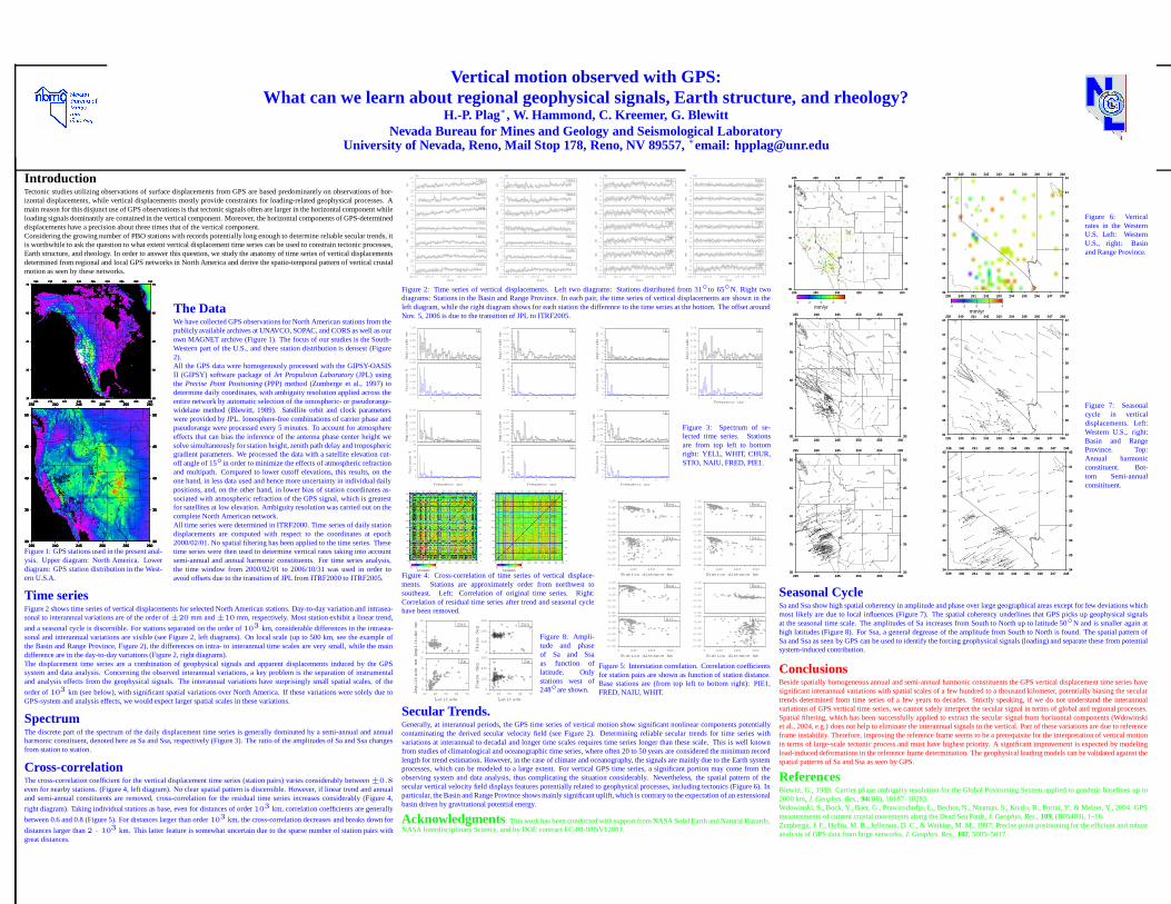
IntroductionTectonic studies utilizing observations of surface displacements from GPS are based predominantly on observations of hor-izontal displacements, while vertical displacements mostly provide constraints for loading-related geophysical processes. Amain reason for this disjunct use of GPS observations is that tectonic signals often are larger in the horizontal component whileloading signals dominantly are contained in the vertical component. Moreover, the horizontal components of GPS-determineddisplacements have a precision about three times that of the vertical component.Considering the growing number of PBO stations with records potentially long enough to determine reliable secular trends, itis worthwhile to ask the question to what extent vertical displacement time series can be used to constrain tectonic processes,Earth structure, and rheology. In order to answer this question, we study the anatomy of time series of vertical displacementsdetermined from regional and local GPS networks in North America and derive the spatio-temporal pattern of vertical crustalmotion as seen by these networks.

15

30

45

60

75

15

30

45

60

75

195 210 225 240 255 270 285 300 315

195 210 225 240 255 270 285 300 315

15

30

45

60

75

15

30

45

60

75

195 210 225 240 255 270 285 300 315

195 210 225 240 255 270 285 300 315

15

30

45

60

75

15

30

45

60

75

195 210 225 240 255 270 285 300 315

195 210 225 240 255 270 285 300 315

15

30

45

60

75

15

30

45

60

75

195 210 225 240 255 270 285 300 315

195 210 225 240 255 270 285 300 315

15

30

45

60

75

15

30

45

60

75

195 210 225 240 255 270 285 300 315

195 210 225 240 255 270 285 300 315

30

35

40

45

50

30

35

40

45

50

235 240 245 250 255 260

235 240 245 250 255 260

30

35

40

45

50

30

35

40

45

50

235 240 245 250 255 260

235 240 245 250 255 260

30

35

40

45

50

30

35

40

45

50

235 240 245 250 255 260

235 240 245 250 255 260

30

35

40

45

50

30

35

40

45

50

235 240 245 250 255 260

235 240 245 250 255 260

30

35

40

45

50

30

35

40

45

50

235 240 245 250 255 260

235 240 245 250 255 260

Figure 1: GPS stations used in the present anal-ysis. Upper diagram: North America. Lowerdiagram: GPS station distribution in the West-ern U.S.A.

The DataWe have collected GPS observations for North American stations from thepublicly available archives at UNAVCO, SOPAC, and CORS as well as ourown MAGNET archive (Figure 1). The focus of our studies is the South-Western part of the U.S., and there station distribution is densest (Figure2).All the GPS data were homogenously processed with the GIPSY-OASISII (GIPSY) software package of Jet Propulsion Laboratory (JPL) usingthe Precise Point Positioning (PPP) method (Zumberge et al., 1997) todetermine daily coordinates, with ambiguity resolution applied across theentire network by automatic selection of the ionospheric- or pseudorange-widelane method (Blewitt, 1989). Satellite orbit and clock parameterswere provided by JPL. Ionosphere-free combinations of carrier phase andpseudorange were processed every 5 minutes. To account for atmosphereeffects that can bias the inference of the antenna phase center height wesolve simultaneously for station height, zenith path delay and troposphericgradient parameters. We processed the data with a satellite elevation cut-off angle of 15◦in order to minimize the effects of atmospheric refractionand multipath. Compared to lower cutoff elevations, this results, on theone hand, in less data used and hence more uncertainty in individual dailypositions, and, on the other hand, in lower bias of station coordinates as-sociated with atmospheric refraction of the GPS signal, which is greatestfor satellites at low elevation. Ambiguity resolution was carried out on thecomplete North American network.All time series were determined in ITRF2000. Time series of daily stationdisplacements are computed with respect to the coordinates at epoch2000/02/01. No spatial filtering has been applied to the time series. Thesetime series were then used to determine vertical rates taking into accountsemi-annual and annual harmonic constituents. For time series analysis,the time window from 2000/02/01 to 2006/10/31 was used in order toavoid offsets due to the transition of JPL from ITRF2000 to ITRF2005.

Time seriesFigure 2 shows time series of vertical displacements for selected North American stations. Day-to-day variation and intrasea-sonal to interannual variations are of the order of ±20 mm and ±10 mm, respectively. Most station exhibit a linear trend,

and a seasonal cycle is discernible. For stations separated on the order of 103 km, considerable differences in the intrasea-sonal and interannual variations are visible (see Figure 2, left diagrams). On local scale (up to 500 km, see the example ofthe Basin and Range Province, Figure 2), the differences on intra- to interannual time scales are very small, while the maindifference are in the day-to-day variations (Figure 2, right diagrams).The displacement time series are a combination of geophysical signals and apparent displacements induced by the GPSsystem and data analysis. Concerning the observed interannual variations, a key problem is the separation of instrumentaland analysis effects from the geophysical signals. The interannual variations have surprisingly small spatial scales, of the

order of 103 km (see below), with significant spatial variations over North America. If these variations were solely due toGPS-system and analysis effects, we would expect larger spatial scales in these variations.

SpectrumThe discrete part of the spectrum of the daily displacement time series is generally dominated by a semi-annual and annualharmonic constituent, denoted here as Sa and Ssa, respectively (Figure 3). The ratio of the amplitudes of Sa and Ssa changesfrom station to station.

Cross-correlationThe cross-correlation coefficient for the vertical displacement time series (station pairs) varies considerably between ±0.8

even for nearby stations. (Figure 4, left diagram). No clear spatial pattern is discernible. However, if linear trend and annualand semi-annual constituents are removed, cross-correlation for the residual time series increases considerably (Figure 4,

right diagram). Taking individual stations as base, even for distances of order 103 km, correlation coefficients are generally

between 0.6 and 0.8 (Figure 5). For distances larger than order 103 km, the cross-correlation decreases and breaks down for

distances larger than 2 · 103 km. This latter feature is somewhat uncertain due to the sparse number of station pairs with

great distances.

PIE1

2000.00 2001.60 2003.20 2004.80 2006.40

Year

-50

0

50

100

mm

FRED

-50

0

50

100

mm

NAIU

-50

0

50

100

mm

STJO

-50

0

50

100

mm

CHUR

-50

0

50

100

mm

WHIT

-50

0

50

100

mm

YELL

-50

0

50

100

mm

Up

PIE1

2000.00 2001.60 2003.20 2004.80 2006.40

Year

-50

0

50

100

mm

FRED

-50

0

50

100

mm

NAIU

-50

0

50

100

mm

STJO

-50

0

50

100

mm

CHUR

-50

0

50

100

mm

WHIT

-50

0

50

100

mm

YELL

-50

0

50

100

mm

Up

FERN

2000.00 2001.60 2003.20 2004.80 2006.40

Year

-45

-15

15

45

mm

SHOS

-45

-15

15

45

mm

APEX

-45

-15

15

45

mm

FRED

-45

-15

15

45

mm

ALAM

-45

-15

15

45

mm

ECHO

-45

-15

15

45

mm

RAIL

-45

-15

15

45

mm

Up

FERN

2000.00 2001.60 2003.20 2004.80 2006.40

Year

-45

-15

15

45

mm

SHOS

-45

-15

15

45

mm

APEX

-45

-15

15

45

mm

FRED

-45

-15

15

45

mm

ALAM

-45

-15

15

45

mm

ECHO

-45

-15

15

45

mm

RAIL

-45

-15

15

45

mm

Up

Figure 2: Time series of vertical displacements. Left two diagrams: Stations distributed from 31◦to 65◦N. Right twodiagrams: Stations in the Basin and Range Province. In each pair, the time series of vertical displacements are shown in theleft diagram, while the right diagram shows for each station the difference to the time series at the bottom. The offset aroundNov. 5, 2006 is due to the transition of JPL to ITRF2005.

V

0 2 4 6 8 10

Frequency cpy

0.00

1.80

3.60

5.40

7.20

9.00

Variance %

A

0.00

1.40

2.80

4.20

5.60

7.00

Amplitude mm

V

0 2 4 6 8 10

Frequency cpy

0

4

8

12

16

20

Variance %

A

0.00

1.60

3.20

4.80

6.40

8.00

Amplitude mm

V

0 2 4 6 8 10

Frequency cpy

0

4

8

12

16

20

Variance %

A

0

4

8

12

16

20

Amplitude mm

V

0 2 4 6 8 10

Frequency cpy

0.00

1.60

3.20

4.80

6.40

8.00

Variance %

A

0.00

0.80

1.60

2.40

3.20

4.00

Amplitude mm

V

0 2 4 6 8 10

Frequency cpy

0

6

12

18

24

30

Variance %

A

0.00

1.60

3.20

4.80

6.40

8.00

Amplitude mm

V

0 2 4 6 8 10

Frequency cpy

0

4

8

12

16

20

Variance %

A

0.00

1.40

2.80

4.20

5.60

7.00

Amplitude mm

V

0 2 4 6 8 10

Frequency cpy

0

4

8

12

16

20

Variance %

A

0.00

1.40

2.80

4.20

5.60

7.00

Amplitude mm

Figure 3: Spectrum of se-lected time series. Stationsare from top left to bottomright: YELL, WHIT, CHUR,STJO, NAIU, FRED, PIE1.

0

20

40

60

80

100

120

140

160

180

200

0

20

40

60

80

100

120

140

160

180

200

0 20 40 60 80 100 120 140 160 180 200

0 20 40 60 80 100 120 140 160 180 200

-0.2 0.1 0.4 0.7 1.0

Correlation

0

20

40

60

80

100

120

140

160

180

200

0

20

40

60

80

100

120

140

160

180

200

0 20 40 60 80 100 120 140 160 180 200

0 20 40 60 80 100 120 140 160 180 200

-0.2 0.1 0.4 0.7 1.0

Correlation

Figure 4: Cross-correlation of time series of vertical displace-ments. Stations are approximately order from northwest tosoutheast. Left: Correlation of original time series. Right:Correlation of residual time series after trend and seasonal cyclehave been removed.

Sa

30 40 50 60 70

Latitude

0

4

8

12

Amplitude mm Sa

30 40 50 60 70

Latitude

0

120

240

360

Phase deg

Ssa

0

4

8

12

Amplitude mm Ssa

0

120

240

360

Phase deg

Figure 8: Ampli-tude and phaseof Sa and Ssaas function oflatitude. Onlystations west of248◦are shown.

Ori.

0 1200 2400 3600

Station distance km

-1.00

-0.60

-0.20

0.20

0.60

1.00

Res.

-1.00

-0.60

-0.20

0.20

0.60

1.00

Ori.

0 1200 2400 3600

Station distance km

-1.00

-0.60

-0.20

0.20

0.60

1.00

Res.

-1.00

-0.60

-0.20

0.20

0.60

1.00

Ori.

0 1200 2400 3600

Station distance km

-1.00

-0.60

-0.20

0.20

0.60

1.00

Res.

-1.00

-0.60

-0.20

0.20

0.60

1.00

Ori.

0 1200 2400 3600

Station distance km

-1.00

-0.60

-0.20

0.20

0.60

1.00

Res.

-1.00

-0.60

-0.20

0.20

0.60

1.00

Figure 5: Interstation correlation. Correlation coefficientsfor station pairs are shown as function of station distance.Base stations are (from top left to bottom right): PIE1,FRED, NAIU, WHIT.

Secular Trends.Generally, at interannual periods, the GPS time series of vertical motion show significant nonlinear components potentiallycontaminating the derived secular velocity field (see Figure 2). Determining reliable secular trends for time series withvariations at interannual to decadal and longer time scales requires time series longer than these scale. This is well knownfrom studies of climatological and oceanographic time series, where often 20 to 50 years are considered the minimum recordlength for trend estimation. However, in the case of climate and oceanography, the signals are mainly due to the Earth systemprocesses, which can be modeled to a large extent. For vertical GPS time series, a significant portion may come from theobserving system and data analysis, thus complicating the situation considerably. Nevertheless, the spatial pattern of thesecular vertical velocity field displays features potentially related to geophysical processes, including tectonics (Figure 6). Inparticular, the Basin and Range Province shows mainly significant uplift, which is contrary to the expectation of an extensionalbasin driven by gravitational potential energy.

30

35

40

45

50

30

35

40

45

50

235 240 245 250 255 260

235 240 245 250 255 260

-4 -2 0 2 4

mm/yr

30

35

40

45

50

30

35

40

45

50

235 240 245 250 255 260

235 240 245 250 255 260

34

35

36

37

38

39

40

41

42

34

35

36

37

38

39

40

41

42

239 240 241 242 243 244 245 246 247 248

239 240 241 242 243 244 245 246 247 248

-4 -2 0 2 4

mm/yr

34

35

36

37

38

39

40

41

42

34

35

36

37

38

39

40

41

42

239 240 241 242 243 244 245 246 247 248

239 240 241 242 243 244 245 246 247 248

Figure 6: Verticalrates in the WesternU.S. Left: WesternU.S., right: Basinand Range Province.

30

35

40

45

50

30

35

40

45

50

235 240 245 250 255 260

235 240 245 250 255 260

30

35

40

45

50

30

35

40

45

50

235 240 245 250 255 260

235 240 245 250 255 260

30

35

40

45

50

30

35

40

45

50

235 240 245 250 255 260

235 240 245 250 255 260

30

35

40

45

50

30

35

40

45

50

235 240 245 250 255 260

235 240 245 250 255 260

34

35

36

37

38

39

40

41

42

34

35

36

37

38

39

40

41

42

239 240 241 242 243 244 245 246 247 248

239 240 241 242 243 244 245 246 247 248

34

35

36

37

38

39

40

41

42

34

35

36

37

38

39

40

41

42

239 240 241 242 243 244 245 246 247 248

239 240 241 242 243 244 245 246 247 248

34

35

36

37

38

39

40

41

42

34

35

36

37

38

39

40

41

42

239 240 241 242 243 244 245 246 247 248

239 240 241 242 243 244 245 246 247 248

34

35

36

37

38

39

40

41

42

34

35

36

37

38

39

40

41

42

239 240 241 242 243 244 245 246 247 248

239 240 241 242 243 244 245 246 247 248

Figure 7: Seasonalcycle in verticaldisplacements. Left:Western U.S., right:Basin and RangeProvince. Top:Annual harmonicconstituent. Bot-tom Semi-annualconsitituent.

Seasonal CycleSa and Ssa show high spatial coherency in amplitude and phase over large geographical areas except for few deviations whichmost likely are due to local influences (Figure 7). The spatial coherency underlines that GPS picks up geophysical signalsat the seasonal time scale. The amplitudes of Sa increases from South to North up to latitude 50◦N and is smaller again athigh latitudes (Figure 8). For Ssa, a general degrease of the amplitude from South to North is found. The spatial pattern ofSa and Ssa as seen by GPS can be used to identify the forcing geophysical signals (loading) and separate these from potentialsystem-induced contribution.

ConclusionsBeside spatially homogeneous annual and semi-annual harmonic constituents the GPS vertical displacement time series havesignificant interannual variations with spatial scales of a few hundred to a thousand kilometer, potentially biasing the seculartrends determined from time series of a few years to decades. Strictly speaking, if we do not understand the interannualvariations of GPS vertical time series, we cannot safely interpret the secular signal in terms of global and regional processes.Spatial filtering, which has been successfully applied to extract the secular signal from horizontal components (Wdowinskiet al., 2004, e.g.) does not help to eliminate the interannual signals in the vertical. Part of these variations are due to referenceframe instability. Therefore, improving the reference frame seems to be a prerequisite for the interpretation of vertical motionin terms of large-scale tectonic process and must have highest priority. A significant improvement is expected by modelingload-induced deformations in the reference frame determination. The geophysical loading models can be validated against thespatial patterns of Sa and Ssa as seen by GPS.

ReferencesBlewitt, G., 1989. Carrier phase ambiguity resolution for the Global Positioning System applied to geodetic baselines up to2000 km, J. Geophys. Res., 94(B8), 10187–10283.Wdowinski, S., Bock, Y., Baer, G., Prawirodirdjo, L., Bechor, N., Naaman, S., Knafo, R., Forrai, Y., & Melzer, Y., 2004. GPSmeasurements of current crustal movements along the Dead Sea Fault, J. Geophys. Res., 109, (B05403), 1–16.Zumberge, J. F., Heflin, M. B., Jefferson, D. C., & Watkins, M. M., 1997. Precise point positioning for the efficient and robustanalysis of GPS data from large networks, J. Geophys. Res., 102, 5005–5017.

Acknowledgments: This work has been conducted with support from NASA Solid Earth and Natural Hazards,NASA Interdisciplinary Science, and by DOE contract FC-08-98NV12081.