vertical integration and risk management in competitive

Vertical Integration and Risk Management in CompetitiveMarkets of Non-Storable Goods ∗

René Aïd† Arnaud Porchet‡ Nizar Touzi§

29th September 2006

Abstract

This paper provides an analysis of vertical integration and its benefits for riskdiversification in competitive markets of non-storable goods. We study the interactionsbetween spot, forward and retail markets, and the impact of vertical integration onthese interactions. In this setting, we present an equilibrium model for the threemarkets, where a set of actors are specialized in upstream or downstream segmentsor both if they are integrated. They must decide at time t = 0 their retail marketshare and forward positions under uncertainty before time t = 1 where productionand supply occur. The objective of each actor is to maximize a mean-variance utilityfunction, and the equilibrium can be characterized explicitly.We show that vertical integration and forward hedging are two levers for diversifyingdemand and spot prices risks. We prove that they exhibit similar properties relativelyto their impact on retail prices and actors’ utility. We also show that, in the presence ofhighly risk averse downstream actors, vertical integration is more efficient to diversifyrisk.

Keywords: Electricity Market, Spot, Forward, Retail, Perfect Competition, Equilib-rium, Mean Variance Utility, Market Share, Hedging, Production Management, VerticalIntegration, Risk.

∗Acknowledgement. The authors are grateful to Profs. Jean Tirole, Robert B. Wilson and G.Chemla for their helpful comments. The paper also benefited from numerous discussions with JérômeWirth and Cyrille Strugarek at EDF R&D.

†EDF R&D - Département OSIRIS. 1, avenue du Général de Gaulle, F-92141 Clamart CedexFRANCE. Tel: 33 (0)1 47 65 46 86, email: [email protected]

‡Corresponding author. Université Paris Dauphine CEREMADE, ENSAE CREST and EDFR&D. EDF R&D - Département OSIRIS, 1, avenue du Général de Gaulle, F-92141 Clamart CedexFRANCE. Tel: 33 (0)1 47 65 36 71, email: [email protected]

§Centre de Mathématiques Appliquées, Ecole Polytechnique Paris, France, and Imperial CollegeLondon. [email protected]

1

1 Introduction

Understanding the determinants of vertical integration has been the focus of much atten-tion and a unified theory has still not emerged. This question has been clarified fromseveral different perspectives, all of which virtually rely on some form of imperfections(see for instance the surveys by Perry [17] and Joskow [13]). In particular, the presenceof uncertainties has been proved to be an argument in favor of vertical integration. InWilliamson [18] or Bolton and Whinston [5], contractual incompleteness makes it moreefficient to integrate vertically. Indeed, long-term contracts can be costly and difficult, ifnot impossible, to specify in every possible state of the world. Opportunistic behaviours,appearing when the contractual relations are misspecified, induce inefficiencies. Verticalintegration then allows for cooperative adaptation, better decision-making and risk re-duction. Arrow [3] develops a model in which vertical integration is sought for acquiringvaluable private information about the production process. In Green [11] firms integratevertically to avoid rationing. In Hendrikse and Peters [12] and Carlton [6], uncertaintyin demand, rationing, lack of market flexibility and risk aversion are the determinants ofvertical integration. When markets are competitive and in the absence of frictions, riskdiversification can still be a reason for integration, as showed in Perry [17]. In Emons [9],downstream firms integrate upwards to ensure supply at a lower price.As mentioned above, long-term contracts are a common alternative to vertical integration.They are theoretically more flexible means of ensuring supply and price stability but areusually difficult to write thus leading to complex and sometimes misspecified contracts.Relations between vertical integration and long-term contracts have been studied by Klein[15] and Joskow [14] from the point of view of incomplete contracts. In the special case ofelectricity markets, Chao, Oren and Wilson argue in [7]-[8] that a certain level of verticalintegration is efficient when the market fails to provide a full set of hedging instruments.

The main objective of this paper is to clarify and quantify the impact of vertical inte-gration from the point of view of risk diversification and discuss the similarities betweenvertical integration and long-term contracts. We aim at understanding the fundamentalmechanisms of risk diversification operating in retail, forward and spot markets, togetherwith the relationship linking each market’s equilibrium price. We only focus on risk anddo not consider either strategic behavior nor market power. Therefore we concentrate onperfectly competitive markets and are guaranteed that risk diversification considerationsare completely responsible for the properties of our equilibrium analysis. We also ignoreany kind of profit sharing rules other than vertical integration.To this end, we develop an equilibrium model of perfectly competitive retail, forward andspot markets for a non-storable good. At time t = 0, downstream firms (or downstreamsubsidiaries of integrated firms) choose their retail market shares and forward positions fortime t = 1. At that time, upstream firms (or downstream subsidiaries) produce the good,

2

sell it to downstream entities on the spot market, which deliver it to end-customers. Wesuppose that the final demand is random and inelastic and that uncertainty is revealed attime t = 1 before production occurs. Decisions at time t = 0 must then be taken underuncertain demand and spot price. We suppose that the good is non-storable so that noproduction can occur at time t = 0 and be stored until time t = 1. This corresponds to themodels studied by Allaz [1] or Bessembinder and Lemmon [4], where we consider in addi-tion the retail activity. Assuming that agents’ preferences are defined by a mean-varianceutility function and that they disregard any influence they could have on the equilibriumprice or on the other actors’ decisions, we derive the equilibrium prices and exchangedquantities on the three markets in closed forms.

In this setting, we show that vertical integration and forward hedging are two levers forachieving risk diversification, that exhibit similar properties. First, they both have a down-ward impact on retail price. Second, they are both means for actors with low generationcapacity to corner larger market shares. Third, they both tend to decrease downstreamfirms’ utility when upstream firms are only partially integrated. Fourth, the impact of oneof these levers one retail price and utilities is drastically reduced in the presence of theother. Nevertheless, we also observe some discrepancies between these two levers due toa strong asymmetry between upstream and downstream firms in terms of risk. Indeed,downstream firms have to take decisions under uncertainty, while upstream firms respondto it. In addition, in the absence of forward hedging, vertical integration and demandelasticity, profit of upstream firms are not impacted by retail price, whereas downstreamrevenues are impacted by spot price. Therefore, downstream firms are more exposed torisk. As a consequence, we observe that, first, vertical integration restores this symmetrywhile forward hedging does not. Second, vertical integration is more robust towards highrisk aversions in the sense that it can achieve risk diversification when forward hedgingfails. Third, vertical integration can also increase downstream firms’ utility provided thatthey have sufficiently high risk aversion. Fourth, a non-integrated economy can be a stableequilibrium whereas a situation where no actors trade forward contracts is almost neverstable a stable equilibrium. Finally, we prove that the inelasticity assumption of demandto retail price is not restrictive and that our conclusions prevail in this setting.The paper is organized as follows. We formulate the equilibrium problem in Section 2, andcompare two different situations. First, in Section 3, we consider the equilibrium whenthere is no forward market. Then, in Section 4, we introduce the forward market and solvethe associated equilibrium problem. After having developed the model, we illustrate inSection 5 some case studies in the electricity sector with data from the French market.Finally, in Section 6.1, we discuss the extension of the model to the case of an elasticdemand.

3

2 The model

In this section we describe perfectly competitive retail, forward and spot markets for anon-storable good, and define an equilibrium on these markets.

2.1 The markets

We consider a set P of producers of a non-storable good (upstream firms) selling theirproduction on spot and forward wholesale markets. A set R of retailers (downstreamfirms) sources on the markets and delivers the good to end-customers, whose demand isdenoted by D. We also suppose that all actors have access to wholesale markets and weallow for the presence of purely speculative actors (traders) who have no production norretail subsidiaries. We denote by K the set of all actors: producers, retailers and traders.We emphasize the fact that an actor is not necessarily specialized in a single activity,but can own subsidiaries of different kinds. Hence the subsets P and R of K are possiblyintersecting, leading to four different kinds of actors: pure retailers who buy on the marketsand deliver to end-customers, pure producers who produce and sell their production onthe wholesale markets, pure traders who only speculate between the spot and forwardmarkets, and integrated producers who produce, trade on the markets and also deliver toend-customers.There are two dates in the model: t = 0 and t = 1. We suppose that demand D israndom, inelastic and corresponds to the demand at the future date t = 1 (we discussthe case of elastic demand in Section 6.1). Since the good is non-storable, productioncan only occur at that time t = 1 when the demand uncertainty is observed. Demandcannot be served by producing at time t = 0 and storing the good until time t = 1. Onthe other hand, decisions regarding forward and retail contracts must be made at timet = 0, before demand uncertainty is revealed. We suppose here that a single product isoffered to all retail customers, that these customers are indifferent as to the choice of aretailer and are only concerned with the level of retail price. We finally assume a perfectlycompetitive environment: all actors compete disregarding any influence they could haveon the equilibrium price, or the other actors’ behaviour.

In Subsection 6.2 we consider the case where decisions on the retail and forward marketare not taken simultaneously. We prove that, under the assumption of competitive markets,the equilibrium remains unchanged if forward market decisions are taken prior to retailmarket decisions or vice-versa.

At time t = 0, downstream firms choose their market shares αk ∈ [0, 1], k ∈ R. Wedenote by p the retail price. Demand satisfaction at time t = 1 imposes the market-clearing

4

constraint:

1 =∑k∈R

αk . (2.1)

The actors also take positions on the forward market at that date. We denote by q theforward price and by fk, k ∈ K, the forward positions (where fk > 0 represents a purchase).We also assume a perfectly competitive forward market where the actors must meet themarket-clearing constraint:

0 =∑k∈K

fk . (2.2)

Finally, at time t = 1, when demand uncertainty is resolved, the actors take positions onthe spot market. We denote by P the spot price and by Gk, k ∈ K, the spot positions(where Gk > 0 represents a purchase). As in the case of retail and forward markets, it isassumed that the actors follow the rules of perfect competition on the spot market. Themarket-clearing constraint reads:

0 =∑k∈K

Gk . (2.3)

Together with the spot positions, producers choose their generation levels Sk, k ∈ P, thatmust meet demand D:

D =∑k∈P

Sk . (2.4)

Each actor aims at maximizing its profit, i.e. sum of its gains on the retail, forward andspot markets minus its production costs:

pαkD1k∈R − qfk − PGk − ck (Sk)1k∈P .

Non-storability imposes that the net volume of good bought, sold or produced by actor k

is zero (no inventory is possible):

0 = αkD1k∈R − fk −Gk − Sk1k∈P ,

allowing us to discard variable Gk and write the profit function as:

(p− P )αkD1k∈R + (P − q)fk + (PSk − ck (Sk))1k∈P .

Three terms appear in this expression. The first one is the profit made by a retailer whosatisfies a demand αkD at retail price p by sourcing on the spot market at price P . Thesecond one is the profit made by a trader buying a volume fk on the forward market atprice q and selling it on the spot market at price P . The third term is the profit made bya producer who generates a volume Sk at cost ck(Sk) and sells it on the spot market atprice P .

5

We finally suppose that the preferences of actor k are described by a mean-varianceutility function with risk aversion coefficient λk. We will use the following notation for themean variance utility function:

MVλk[ξ] := E[ξ]− λkVar[ξ] .

Notice that MVλkhas the inconvenience of not being monotonic, which implies possible

negative prices at equilibrium. Nevertheless, as shown in [16], it can always be seen as asecond order expansion of a monotonic Von Neumann-Morgenstern utility function.

2.2 Equilibrium on the spot market

Demand D at time t = 1 is supposed to be exogenous to all actors and totally inelastic toboth retail and spot prices. See Section 6.1 for the extension to elastic demand. DemandD is described by a random variable on a probability space (Ω, F , P). In this setting, theequilibrium on the spot market is straightforward and independent of any decision takenat time t = 0. For this reason, we start the analysis with this market.

Each producer k ∈ P is characterized by a cost function x 7→ ck(x) defined on R+ andsatisfying the Inada conditions:

c′k(0+) = 0, c′k(+∞) = +∞ . (2.5)

We also suppose that the functions ck are continuously differentiable and strictly convex.The cost ck(x) represents the cost for actor k to produce a quantity x. Producer k’sgeneration profit on the spot market reads:

PSk − ck(Sk) . (2.6)

At time t = 1, when entering the spot market, the actors know the realization of demanduncertainty D, and decisions on the retail and forward markets have already been taken.The spot market competitive equilibrium is thus classically given by:

P ∗ = C ′(D) , S∗k = (c′k)

−1(P ∗) , (2.7)

where the aggregate cost function C is defined by:

C(x) :=∑k∈P

ck (c′k)−1

(∑k∈P

(c′k)−1

)−1

(x) ,

and verifies:

C ′(x) =

(∑k∈P

(c′k)−1

)−1

(x) ,

6

so that the random variable

C(D) =∑k∈P

ck (S∗k(P ∗))

is the sum of the production costs over all producers. At equilibrium each producer pro-duces at marginal cost.

The equilibrium on the spot market only depends on the exogenous demand D and istherefore independent of any other equilibrium prior to time t = 1. This results from thenon-storability condition and the inelasticity assumption on D. Note that this situation isdifferent from [1], where the demand elasticity to spot price implies a dependency of thespot price to forward positions and a reduction of the market power of the producers. Inthe following, the equilibrium spot price P ∗ and the generation profit

Πgk := (P ∗S∗

k − ck (S∗k))1k∈P (2.8)

will act as exogenous random variables and we suppose that their distribution is knownby all actors. We then replace variables P and Sk by P ∗ and S∗

k found previously, and wedefine the profit function of actor k

Πk(p, q, αk, fk) := Πrk(p, αk) + Πt

k(q, fk) + Πgk , (2.9)

where Πgk is defined by (2.8) and

Πrk(p, αk) := (p− P ∗)αkD1k∈R (2.10)

Πtk(q, fk) := (P ∗ − q)fk . (2.11)

Here, Πrk is the net retail profit derived from supplying a retail demand by sourcing on the

spot market, and Πtk is the net trading profit earned by buying on the forward market and

selling on the spot market. Finally, Πgk is the net generation profit gained by producing

and selling production on the spot market.

Remark 2.1. The model presented in this article does not actually require the assumptionof inelastic demand and competitive equilibrium on the spot market. It can be handledsimilarly without these assumptions, as soon as the equilibrium on the spot market onlydepends on the retail price. Nonetheless, for clarity purpose, we choose to stick to thisframework and address possible generalizations of the model in Section 6.1. 3

2.3 Competitive Equilibrium

In order to define an equilibrium, we introduce the following two sets:

A :=

(αk)k∈K ∈ [0, 1]|K| : ∀k /∈ R, αk = 0 and

∑k∈K

αk = 1

(2.12)

F :=

(fk)k∈K ∈ R|K| :

∑k∈K

fk = 0

. (2.13)

7

Definition 2.1. An equilibrium of the retail-forward equilibrium problem is a quadruple(p∗, q∗, α∗, f∗) ∈ R+ × R+ ×A× F such that:

(α∗k, f

∗k ) = argmax

αk,fk

MVλk[Πk (p∗, q∗, αk, fk)] , ∀k ∈ K . (2.14)

This defines a simultaneous competitive equilibrium on both markets. Each actor sub-mits a supply function specifying his levels of forward purchase and market share for eachprice level. Each actor chooses his supply function taking the prices as given and withouttaking into account the presence of competitors. Then, the auctioneer collects all supplyfunctions and sets the prices that ensure market clearing and demand satisfaction. SeeSubsection 6.2 for other definitions of the equilibrium that introduce sequentiality betweenforward and retail market.

3 Equilibrium without a forward market

In this section, we focus on equilibria in the absence of a forward market. We derive theexplicit formulation of the equilibrium and analyse the results. In the absence of a forwardmarket, we define the profit function without a forward position:

Π0k(p, αk) := Πk(p, 0, αk, 0) = Πr

k(p, αk) + Πgk .

In this context, definition 2.1 reduces to:

Definition 3.1. An equilibrium of the retail equilibrium problem is a pair (p∗, α∗) ∈R+ ×A such that:

α∗k = argmax

αk

MVλk

[Π0

k (p∗, αk)], ∀k ∈ K . (3.1)

3.1 Characterization of the equilibrium

Let

ΠgI :=

∑k∈R∩P

Πgk (3.2)

be the aggregate generation profit realized by all integrated producers, i.e. firms runningboth generation and supply units, and let

Πr :=∑k∈R

Πrk(p

∗, α∗k) = (p∗ − P ∗)D (3.3)

be the aggregate retail profit realized by all retailers at equilibrium. We also define

Λ :=

(∑k∈K

λ−1k

)−1

, ΛR :=

(∑k∈R

λ−1k

)−1

, (3.4)

8

which can be interpreted as the aggregate risk aversion coefficients, respectively for the setof all actors and the set of all retailers. Parameter λ−1

k corresponds to the risk toleranceof actor k, as defined in [10]. Our equilibrium problem is similar on each market to thatfaced by syndicates in [19], where an aggregate risk tolerance is defined by summing overthe risk tolerances of the syndicate members, in agreement with (3.4).

We only focus on interior equilibria, i.e. equilibria where constraints α∗ ∈ [0, 1] andp∗ ≥ 0 are not binding, by discarding cases where some retailers in R have null marketshares. The equilibrium is then characterized by the following proposition.

Proposition 3.1. (p∗, α∗) ∈ R∗+ × int(A) defines an equilibrium of the retail equilibrium

problem without a forward market iff:

α∗k =

ΛRλk

+ΛRλk

Cov[Πr,ΠgI ]

Var[Πr]−

Cov[Πr,Πgk]

Var[Πr], (3.5)

and p∗ solves the second order polynomial equation:

0 = E[(p∗ − P ∗)D]− 2ΛRCov[(p∗ − P ∗)D, (p∗ − P ∗)D + ΠgI ] . (3.6)

Proof. See Appendix A 2

3.2 Equilibrium retail price

Having now an explicit formulation of the equilibrium, we analyse the retail price proper-ties.

Risk neutral case and uniqueness. First, we observe that the retail price is charac-terized by a second order polynomial in (3.6). This equation may have several solutionsor none, thus existence and uniqueness are not guaranteed a priori, as a drawback of themean-variance analysis. We next argue that, if there exists two solutions, only one is rele-vant.For this purpose, we start the analysis with the risk neutral case. If some retailer is riskneutral, i.e. λk0 = 0 for some k0 ∈ R, the equilibrium retail price reduces to:

p0 =E[P ∗D]

E[D], (3.7)

Since P ∗ = C ′(D) is a non-decreasing function of D, implying that P ∗ and D are positivelycorrelated, we deduce that the risk neutral retail price is greater than the expected spotprice:

p0 ≥ E[P ∗] .

Suppose now that all retailers are risk-averse. It seems natural to expect the equilibriumretail price to tend to the risk neutral price when the risk aversion coefficient of some retailer

9

tends to zero. In this case, the aggregate risk aversion coefficient ΛR also becomes zero.Suppose equation (3.6) has two non-negative solutions p− ≤ p+. The Taylor expansion ofthese roots around ΛR = 0 reads:

p− ' p0 +2ΛR

E[D]Var[D]

(Var[D]Cov[PD,PD −Πg

I ]− Cov2[D,PD − 12Πg

I ]

+2Cov2[D,PD − 12Πg

I − p0D])

p+ ' E[D]2ΛRVar[D]

.

This shows that p− tends to p0 as ΛR tends to 0, while p+ tends to infinity. For this reason,the following analysis considers that p− is the relevant root from the economic point ofview, and the equilibrium is in fact uniquely characterized.

Impact of integration. Let us consider the impact of vertical integration on the equi-librium retail price. We prove that the presence of integrated producers has a downwardimpact on retail price. To this end, we denote by p∗NI the smallest solution of (3.6) in theabsence of integrated producers, and by p∗I in the presence of some integrated producers.Suppose that R∩P = ∅, i.e. there are no integrated producers who have both generationand supplying activities. Equation (3.6) then reduces to:

0 = E[(p∗NI − P ∗)D]− 2ΛRVar[(p∗NI − P ∗)D] . (3.8)

As a consequence, it is also greater than the expected spot price.When some actors are integrated, i.e. R ∩ P 6= ∅, the equation that determines theequilibrium price is

0 = E[(p∗I − P ∗)D]− 2ΛRCov[(p∗I − P ∗)D, (p∗I − P ∗)D + ΠgI ] .

Suppose one retailer, whom we will name i, decides to become an integrated producer. Inthis case, ΛR is unchanged and Πg

I = Πgi . Suppose also that Πr and Πg

I are negativelycorrelated. We then obtain:

0 ≥ E[(p∗I − P ∗)D]− 2ΛRVar[(p∗I − P ∗)D] . (3.9)

This last assumption concerning the correlation of Πr and ΠgI is natural. Since P ∗ =

C ′(D), profit Πgk is an increasing function of D. We cannot prove that the retail profit

Πr = (p∗−P ∗)D is a decreasing function of D but as p∗ is a fixed price and P ∗ is increasingwith D, we have the intuition that Πr will decrease with D. This justifies the negativityassumption on the covariance of Πr and Πg

I . The numerical application performed inSection 5 confirms this intuition.Previous inequality (3.9), confronted to (3.8), shows that p∗I is smaller than p∗NI . Integratedfirms then have a downward impact on retail price.

10

3.3 Equilibrium market shares

We turn to the analysis of market shares properties at equilibrium.

Risk neutral case. The equilibrium market shares of the risk averse retailers are givenby:

α0k = −

Cov[Πr,Πgk]

Var[Πr], (3.10)

while the remaining demand is split among the risk neutral retailers. In particular, arisk averse retailer who has no generation unit ends up with a null market share. Noticethat, in order to satisfy the non-negativity condition of the market shares, equation (3.10)implies Cov[Πr,Πg

k] ≤ 0. We then have another justification of the assumption made inthe previous subsection.

Impact of integration. We now argue that a supplier can increase its market sharewhen integrating. In the absence of integrated producers and risk-neutral suppliers, theequilibrium market shares are given by:

α∗k =

ΛRλk

.

The market shares are distributed proportionally to the risk tolerances, and only dependon these parameters.If integrated firms enter the market, the pure retailers see their equilibrium market sharesmove to:

α∗k =

ΛRλk

+ΛRλk

Cov[Πr,ΠgI ]

Var[Πr],

while the integrated firms have market shares:

α∗k =

ΛRλk

+ΛRλk

Cov[Πr,ΠgI ]

Var[Πr]−

Cov[Πr,Πgk]

Var[Πr].

Suppose once again that Πr is negatively correlated to ΠgI . The pure retailers then see

their equilibrium market shares decrease while the integrated actors increase their marketshares. Indeed, the latter will decrease their risk by diversification if they invest morein the retail market. We also observe that, although the market shares have changed incomparison to the previous case, the relative market shares among the set of pure retailersremain unchanged:

α∗i

α∗j

=λj

λi.

4 Equilibria with a forward market

We now turn to the characterization of the equilibrium in the presence of a forward market.

11

4.1 Characterization of the equilibria

We still focus on interior equilibria, when the constraints are not binding. We define thefollowing quantity:

Πe :=∑k∈K

Πk(p∗, q∗, α∗k, f

∗k ) = p∗D − C(D) ,

which is the aggregate profit of the whole economy. The equilibrium in the presence of aforward market is characterized by the following proposition.

Proposition 4.1. (p∗, q∗, α∗, f∗) ∈ R∗+×R∗

+× int(A)×F defines an equilibrium of theretail-forward equilibrium problem iff:

f∗k =Λλk

Cov [P ∗,Πe]Var [P ∗]

−Cov

[P ∗,Πg

k

]Var [P ∗]

− α∗k

Cov [P ∗,Πr]Var [P ∗]

(4.1)

α∗k =

ΛRλk

+Cov[P ∗,Πr]

∆Cov

[P ∗,Πg

k −ΛRλk

ΠgI

]− Var[P ∗]

∆Cov

[Πr,Πg

k −ΛRλk

ΠgI

](4.2)

q∗ = E[P ∗]− 2ΛCov[P ∗, p∗D − C(D)] , (4.3)

and p∗ is a root of the second order polynomial equation

0 = E[(p∗ − P ∗)D]− 2ΛRCov[(p∗ − P ∗)D, (p∗ − P ∗)D + ΠgI ] (4.4)

+2ΛRCov[P ∗, (p∗ − P ∗)D]

Var[P ∗]Cov

[P ∗, (p∗ − P ∗)D + Πg

I −Λ

ΛR(p∗D − C(D))

],

where

∆ := Var[P ∗]Var[Πr]− Cov2[P ∗,Πr] . (4.5)

Proof. See Appendix A. 2

Having explicitly solved the equilibrium problem, we can analyse the properties of equi-librium prices and positions on the retail and forward markets.

4.2 Equilibrium forward price

The equilibrium forward price is given by:

q∗ = E[P ∗]− 2ΛCov[P ∗,Πe] .

It is equal to the expectation of the spot price corrected by a risk premium term accountingfor the correlation between spot price and global profit Πe at equilibrium, and the aggregaterisk aversion of the market. This kind of formula is typical in the mean-variance utilitybased equilibria, as shown first in [1]. We can also write:

q∗ = E[ZP ∗] with Z := 1− 2Λ(Πe − E[Πe]) .

12

If Λ is small enough so that Z is always strictly positive, Z defines a change of probabilityand q∗ is given by the expectation under a risk-neutral probability of P ∗.We note that the equilibrium forward price does not depend on the distribution of marketshares or that of generation assets, but only on retail and spot equilibrium prices. Moreover,if some traders are risk neutral, the forward price reduces to the expected spot price:

q0 = E[P ∗] .

In the context of quadratic cost functions ck(x) := 12x(akx + bk), ak, bk > 0, q∗ has the

following expression:

q∗ = E[P ∗]− 2Λa

Var[P ∗](p∗ − E[P ∗]) +Λa

Var32 [P ∗]Skew[P ∗] ,

where a−1 :=∑

k∈P a−1k , as presented in [4] in the case of electricity. The forward price

increases with spot price skewness and, in the case where the equilibrium retail price ishigher than the expected spot price, the forward price decreases with spot price volatility.This shows that, in the case of electricity, forward prices lower than the expected spotprice are common since spot price volatility is high for electricity. Nevertheless, forwardprices greater than the expected spot price can occur when spot price skewness is large andpositive, i.e. when large upward peaks are possible. In addition, the equilibrium on theforward market establishes the following relationship between retail and forward prices:

p∗ =E[P ∗]− q∗

2ΛCov[P ∗, D]+

Cov[P ∗, C(D)]Cov[P ∗, D]

.

In particular, higher forward prices correspond to lower retail prices and conversely.

4.3 Equilibrium retail price

The expression of the retail price is more complicated. Nevertheless, the equation givingp∗ in the presence of a forward market is similar to that found in the absence of a forwardmarket. An extra term

2ΛRCov[P ∗, (p∗ − P ∗)D]

Var[P ∗]Cov

[P ∗, (p∗ − P ∗)D + Πg

I −Λ

ΛR(p∗D − C(D))

]is added in the presence of a forward market, but its interpretation is not obvious. We canstill proceed to the Taylor expansion around ΛR = 0 and show that only the smallest rootp∗− of this equation is relevant, ensuring the uniqueness of the equilibrium. We can alsoexhibit the following properties of equilibrium retail prices:

• Risk neutral price. If some retailers are risk neutral, the retail price reduces to:

p0 =E[P ∗D]

E[D],

as in the absence of a forward market.

13

• Price in a fully integrated economy. If all producers are integrated, i.e. P ⊂ R,we obtain:

0 = E[(p∗ − P ∗)D]− 2ΛRCov[(p∗ − P ∗)D, p∗D − C(D)]

+2ΛR

(1− Λ

ΛR

)Cov[P ∗, (p∗ − P ∗)D]

Var[P ∗]Cov[P ∗, p∗D − C(D)] .

In particular, in the absence of pure traders, R = K and Λ = ΛR, so that the aboveequation reduces to (3.6). This means that the forward market has no impact onthe retail price in this case. There is one example where this conclusion is obvious.Suppose there are only N integrated producers, with the same cost function and thesame risk aversion coefficient. By an argument of symmetry, we immediately deriveS∗

k = DN , α∗

k = 1N and f∗k = 0 for all k. The actors do not take any position on the

forward market. The retail price should therefore not be impacted. This conclusionhighlights the symmetry between forward hedging and vertical integration. Whenthe firms already diversify their risk by means of vertical integration, the effect offorward hedging tends to vanish. Conversely, in Subsection 5.2.3, we will see thatin the presence of forward hedging, the level of integration of the actors has littleimpact on retail price.

• Impact of forward trading. In a partially integrated economy, the retail pricebehaviour is not obvious. We can say that p∗F ≤ p∗NF , i.e. retail price in the presenceof a forward market is smaller than in the absence of it, iff

0 ≤(

1− ΛΛR

)Cov2[P ∗, (p∗NF − P ∗)D] + Cov[P ∗, (p∗NF − P ∗)D]Cov[P ∗,Πg

I −Λ

ΛRΠg] .

In particular, this is verified if no producer is integrated and the retail income withouta forward market is negatively correlated to the spot price. This is also verified if noretailer is integrated and Λ = 0 (e.g. existence of a risk-neutral trader). In Subsection5.2, we will see that forward hedging has always a downward impact on retail price,but that its intensity decreases with the level of integration of the actors.

• Impact of integration. Let p∗NI be the equilibrium retail price in the absence ofintegration. In order to compare this price with the equilibrium retail price in thepresence of integrated firms, we substitute p∗NI to p∗ in the right side of (4.4) andstudy the sign of the expression. This leads to studying the sign of:

Cov[P ∗, (p∗NI − P ∗)D]Var[P ∗]

Cov[P ∗,ΠgI ]− Cov[(p∗NI − P ∗)D,Πg

I ].

If we consider as previously the particular case of quadratic cost functions, we obtain:

Cov[P ∗, (p∗NI − P ∗)D]Var[P ∗]

Cov[P ∗,Πgk]− Cov[(p∗NI − P ∗)D,Πg

k]

=a3

2ak

(Var[D2]− Cov2[D2, D]

Var[D]

),

14

which is always positive. This means that the right side of (4.4) is positive for p∗NI

and shows that the equilibrium retail price decreases in the presence of integratedfirms. More generally, we will see in Subsection 5.3 that the presence of verticallyintegrated producers has always a downward impact on retail price. This impact isnonetheless drastically reduced in comparison to the case without a forward market.

4.4 Equilibrium positions on the forward market

In contrast with forward price, equilibrium forward positions do depend on both p∗ andα∗:

f∗k =Λλk

Cov [P ∗,Πe]Var [P ∗]

− α∗k

Cov [P ∗,Πr]Var [P ∗]

−Cov

[P ∗,Πg

k

]Var [P ∗]

. (4.6)

The equilibrium forward position of actor k is composed of three parts. We first notethat if k is a pure speculator, then the last two terms are zero. The first term can thus beinterpreted as the trading component. It is the fraction Λ

λkof a constant term involving the

correlation between the equilibrium global profit and the spot price. An extra supplyingcomponent is added to retailers. It is the fraction α∗

k of a constant term involving thecorrelation between the global retail profit and the spot price. If the retail market revenueis negatively correlated to the spot price, as we argued in the previous section, retailerswill take long positions on the forward market to hedge against high spot prices. Finally,an extra generation component is added to producers, involving the correlation betweentheir generation profit and the spot price. As generation profits are positively correlatedto the spot price, producers will take short forward positions to hedge against low spotprices.

4.5 Equilibrium positions on the retail market

The equilibrium market shares are given by:

α∗k =

ΛRλk

+Cov[P ∗,Πr]

∆Cov

[P ∗,Πg

k −ΛRλk

ΠgI

]− Var[P ∗]

∆Cov

[Πr,Πg

k −ΛRλk

ΠgI

].

In the case where Πgk = ΛR

λkΠg

I for all k ∈ R, the market shares read:

α∗k =

ΛRλk

,

as in a non-integrated economy without a forward market. This is the case when, forexample, there are no integrated firms, or all producers are integrated and generationprofits are proportional to risk tolerances. Another formulation for α∗

k is:

α∗k = α0

k +ΛRλk

(1− Cov[P ∗,Πr]

∆Cov

[P ∗,Πg

I

]+

Var[P ∗]∆

Cov[Πr,Πg

I

]),

15

where

α0k =

Cov[P ∗,Πr]∆

Cov[P ∗,Πg

k

]− Var[P ∗]

∆Cov

[Πr,Πg

k

]is retailer k’s market share in the presence of a risk neutral retailer. This expression allowsfor an analysis of the deviation of market shares from the risk neutral equilibrium.In Section 5, we will observe two important characteristics of market shares. First, thepresence of a forward market is a means for pure retailers to corner larger market shares.Second, the higher the level of integration of an integrated producer, the higher its marketshare.

4.6 Utilities at equilibrium and the strong asymmetry between down-stream and upstream

As mentioned in the introduction, there exists a strong asymmetry in terms of risk betweenretailers and producers. First, in the absence of a forward market and vertical integration,retailers have to take market share decisions under uncertainty, while producers know therealization of demand when they take their generation decision. Second, if the demand isinelastic to retail price, upstream profits are independent of retail price, while downstreamrevenues depend on spot price. This asymmetry is central in our analysis. The examplefor this is the California electricity crisis, where retailers where suffering large losses whileproducers were taking advantage of high spot prices.As a consequence, a pure producer always benefits from trading forward contracts. Indeed,the generation profit Πg

k is an exogenous random variable in this model. As a consequence,when a pure producer bids the strategy fk(q) = 0 for all forward price q, it is guaranteedto receive a utility MVλk

[Πgk], i.e. the utility in the absence of a forward market. Pure

producers thus always enhance their utility in the presence of a forward market because thestrategy f = 0 is admissible and yields the same utility as without one. On the opposite,pure retailers have no guarantee to obtain a higher utility when forward contracts becomeavailable. Indeed, if retailer k decides to bid f = 0, it will receive a utility MVλk

[Πrk].

Nevertheless, the retail profit Πrk depends on p∗, and thus on the other actors’ decisions.

If the retail price p∗ in the presence of forward trading is different from the retail pricewithout forward trading, actor k’s retail profit will change. Not taking position on theforward market will not guarantee it to receive the same utility as in the absence of it. InSubsection 5.2 we observe that the availability of forward contracts decreases pure retailers’utility. Forward contracts are thus not optional in the sense that when they are available,each retailer is individually better off contracting. As a consequence, all retailers trade for-ward contracts and are able to offer lower retail prices. Nevertheless, we observe that thedecrease in expected profit offset that in variance and this risk hedging mechanism impliesa decrease in utility in comparison to the case where no forward contracts are available.The impact of vertical integration on the actors’ utility is difficult to measure. First of all,

16

the question of the evolution of risk aversion with the level of integration has no obviousanswer. One could argue that actors become more or less risk averse when integrating asthe structure itself of the company is affected. This is an open question to define the riskaversion of an integrated actor knowing the risk aversions of the different subsidiaries. Wil-son [19] in his theory of syndicates develops the idea that the risk tolerance of a syndicate,i.e. a group of actors, should be the sum of the actors’ risk tolerance. This idea is alsosuggested in our model, in the way Λ and ΛR are defined. But one could also argue thatthe resulting risk aversion should be the lowest of the subsidiaries’ risk aversions. Indeed,all risky positions would be borne by the least risk averse actor. We illustrate this point inSubsection 5.3. We observe that, like forward hedging, vertical integration decreases theactors’ utility because of a downward impact on retail prices. Nevertheless, for large riskaversions this effect can be opposite and the gain from hedging can be higher than the lossin expected profit. Finally, one obvious aspect of vertical integration is that it breaks theasymmetry between upstream and downstream, and producers’ and retailers’ utilities areimpacted similarly by vertical integration.

5 Application to the electricity industry

In the previous section, we provided theoretical results which can be inferred from theexplicit form of the equilibrium. In order to go further and enhance our understanding ofthe impact of forward trading and vertical integration, we present a serie of case studies,illustrated with historical data of the French electricity market. This market is charac-terized by the presence of a dominant actor, the former monopoly, and recently enteredcompetitors. This situation is far from being compatible with the perfect competitionassumption, but, as we argued above, we are only interested in studying the fundamentalmechanisms of risk diversification, and do not want them to be correlated to market powereffects or strategic behaviors. Nonetheless, a joint study of both components is definitelyof great interest. In the following, we will often study cases involving two actors, who canbe viewed respectively as the former monopoly and the set of competitors.

5.1 Methodology

In this section we aim at computing the retail and forward equilibria using data fromthe French market. Only spot prices and demand levels are publicly available. To haveaccess to the global cost function of the economy, C, we need to know the details of allgeneration assets in the market and all unavailability plannings. As this information is notavailable, we choose to invert the spot price formula P ∗ = C ′(D) to derive a candidatefor C. We use demand and spot price hourly data from December 2004 to March 2005

17

(available respectively on the web site of RTE∗ and Powernext∗∗) as samples for D and P ∗.The winter under consideration was generally mild, but was followed by a wave of intensecold in March. These recordings are showed on Figure 5.1-left. The circles correspond tovalues for March. These are interesting samples as they contain high spot prices and aretherefore indicative of the high volatility observed in the market. Nonetheless they remainstrongly heterogeneous since many generation units were unavailable during March’s coldwave. This implies a cost function C evolving with time. We therefore processed thedata from March 2005 by adding a constant to the demand sample, as suggested by theshape of the plots, to offset the unavailability effect. We then regressed the function C onthese processed samples, so that P ∗ = C ′(D), according to our competitive model (Figure5.1-right). The data for D and P ∗, the risk aversion coefficients and the regressed cost

4 5 6 7 8 9

x 104

0

50

100

150

200

250

300

350

Demand (MW)

Spot

Pric

e (e

uro/

MW

)

Spot and Demand Samples

Dec 2004 − Feb 2005Mar 2005

4.5 5 5.5 6 6.5 7 7.5 8 8.5 9 9.5

x 104

0

50

100

150

200

250

300

350

Demand (MW)

Spot

Pric

e (e

uro/

MW

)

Marginal Cost Curve

P=C’(D)

Figure 5.1: Demand and spot price samples (left). Processed and interpolated data (right).

function C allow us to compute the equilibrium.

Before commenting on the numerical application, we observe that the analysis can be ledwith a limited number of actors without loss of generality. The model involves a numberN of actors. As mentioned in Section 2.1, there are only four types of actors: integratedproducers, pure retailers, pure traders and pure producers. The equilibrium of any N -actor competition is equivalent to an equilibrium involving at most four actors of differentkinds. Indeed, equations (4.1) and (4.2) are linear in λ−1

k and Πgk while (4.4) and (4.3)

only involve the aggregate risk aversion coefficients Λ and ΛR. Hence, N pure retailers ofrisk tolerances λ−1

k can be aggregated into a single pure retailer of risk tolerance∑

k λ−1k .

The equilibrium prices remain unchanged because Λ and ΛR are not impacted, the marketshare of the aggregate retailer is equal to the sum of the market shares by linearity, andthe forward position of the aggregate retailer is equal to the sum of the forward positionsby the same argument. Similarly, N pure producers can be aggregated into a single pureproducer, N pure traders can be aggregated into a single pure trader and N integratedproducers can be aggregated into a single integrated producer. This allows us to only

∗www.rte-france.com∗∗www.powernext.fr

18

consider examples with a limited number of actors in the following subsections, keeping inmind that the associated equilibria are also relevant to more general cases.

5.2 Impact of the forward market

In this paragraph we focus on the impact of forward trading. Therefore, we compare theequilibria with and without a forward market for different configurations of the economyinvolving 2 actors:

1. actor 1 is an integrated producer only facing competition on the retail market2. actor 1, unbundled, becomes a pure producer, while actor 2 is a pure retailer3. actor 1 is integrated and faces the competition of a pure producer4. actor 1 and actor 2 are integrated.

5.2.1 Unbundling of the retail activity

We consider the case where the former monopoly faces competition on the retail market.More precisely, we suppose that the former monopoly is an integrated producer owningall the generation assets, and that all the competitors are pure retailers. According to theremark of the previous paragraph regarding the aggregation of actors, it is equivalent toconsider a two actor competition with one integrated retailer, denoted actor 1, and onepure retailer, actor 2, standing for all the retail competitors. This experiment addresses thequestion of the viability of retail competition in the presence of an integrated generationmonopoly.

In the absence of a forward market, the pure retailer is forced to source on the spotmarket from the integrated producer in order to satisfy its demand. Figure 5.2-left showsactor 1’s market share in this case as a function of the risk aversion coefficients of bothactors. We observe that actor 2 is limited to a very small market share, less than 2%,whatever the values of the risk aversion coefficients of the actors. Actor 2 is in a positionof high financial risk as it is forced to buy on the spot market and is therefore exposed tothe high volatility of spot prices. Actor 2 has therefore very limited possibilities to enterthe retail market, all the more limited as its risk aversion is large. In this context, there islittle incentive for a non-integrated producer to enter the market.Figure 5.2-right shows actor 1’s market share in the presence of a forward market. Dottedmesh regions represent zones where there is no equilibrium (q∗ < 0). In contrast to theprevious case, we observe that if actor 2 is less risk averse than actor 1 then it can enterdeeper in the retail market, up to 40%. The pure retailer can take advantage of its lowerrisk aversion to penetrate the market. We conclude from this example that the presenceof the forward market allows non-integrated producers to contest the retail monopoly.

19

−10

−8

−6

−4

−2

0

−10−8

−6−4

−20

98

98.5

99

99.5

100

log(λ2)

Market Share Actor 1

log(λ1)

α* 1 (%)

−10

−8

−6

−4

−2

0

−10−8

−6−4

−20

50

60

70

80

90

100

log(λ2)


log(λ1)

α* 1 (%)

Figure 5.2: Actor 1’s market share in the absence (left) and presence (right) of the forwardmarket as functions of the logarithm of risk aversion coefficients.

−10 −8 −6 −4 −2 0

−10

−8

−6

−4

−2

038

40

42

44

46

48

log(λ2)

Retail Price

log(λ1)

p* (eur

o/M

Wh)

−10 −8 −6 −4 −2 0

−10

−8

−6

−4

−2

038

40

42

44

46

48

log(λ2)

Retail Price

log(λ1)

p* (eur

o/M

Wh)

Figure 5.3: Equilibrium retail price in the absence (left) and in the presence (right) of theforward market as functions of the logarithm of risk aversion coefficients.

The equilibrium retail price remains unchanged, as we can see on Figure 5.3. This isbecause all producers are integrated (cf. Section 4.3). We can give an interpretation ofthis fact: if all retailers are pure retailers, they will hedge by buying forward contractsto producers, and will be willing to sell at a lower price on the retail market. But if theproducers are also retailers, these integrated producers will take short positions on theforward market and will be willing to increase retail prices. We are then in the presenceof conflicting incentives that offset each other.

We observe that the equilibrium does not always exist in the forward market (dottedmesh zones in Figure 5.4). When both actors are highly risk averse, they do not agreeon exchanging forward. This aspect shows the drawback of the mean-variance utilityfunction. Nonetheless, when the equilibrium exists, actor 2’s forward position is in therange of its expected demand. More precisely, we can state that f2 ' 1.1 α2E[D]: actor 2hedges its retail demand by 10% above the expected demand, whatever its risk aversioncoefficient. This means that the integrated producer is better off being short even if ithas to buy back part of the previously sold volumes on the spot market. We also observe

20

that the equilibrium forward price is almost always greater than the expected spot price(E[P ∗] = 37.9518), at least for sufficiently small risk aversion coefficients.

−10

−8

−6

−4

−2

0

−10−8

−6−4

−20

−4

−3

−2

−1

0x 10

4

log(λ2)

Forward Position Actor 1

log(λ1)

f* 1 (MW

h)

−10−8

−6−4

−20

−10

−8

−6

−4

−2

0

0

10

20

30

40

log(λ2)

Forward Price

log(λ1)

q* (eur

o/M

Wh)

Figure 5.4: Actor 1’s forward position (left) and forward price at equilibrium as functionsof the logarithm of risk aversion coefficients.

−10

−5

0

−10

−5

00

2

4

6

8

10

12

log(λ2)

Excess of Utility Actor 1

log(λ1)

φ ( ∆

U1 )

−10

−5

0

−10

−5

00

2

4

6

8

10

log(λ2)


log(λ1)

φ (∆

U2)

Figure 5.5: Excess of utility for actor 1 (left) and actor 2 (right) as functions of thelogarithm of risk aversion coefficients.

Finally, we observe on Figure 5.5 that the utilities of both actors are higher in thepresence of the forward market. This figure shows for both actors the excess of utility∆U = UF − UNF , induced by the presence of the forward market. For convenience, weplotted the monotonic transform φ(∆U), where φ(x) := sgn(x) log(1 + |x|), in order toshow both the logarithm of ∆U and its sign. In this case, both actors benefit from thepresence of the forward market.For a better understanding of the impact of forward hedging, Table 1 reports the relativeexcesses of utility, average profit and variance (”Risk") on the example λ1 = λ2 = 10−6.We also computed the two following quantities. First, we indicate the ratio “excess ofaverage profit" over “excess of risk", denoted “Profit vs. Risk", and we provide a measureof the excess of performance, the performance being defined by the ratio “expected profit"over risk. We observe that forward trading has a higher impact on actor 2’s utility than onactor 1’s. Actor 1 mainly uses forward contracts for hedging purposes, thus reducing thevariance of its profits by 59 %. The relative loss in average profit associated to this hedging

21

position is low, 0.67 times smaller than the variance reduction, resulting in a slight increasein utility. On the other hand, actor 2 increases both its average profit and risk by 793 %.The average profit increase being twice the risk increase, its utility also increases. Fromthis point of view, forward trading has a higher impact on actor 2’s business. Nevertheless,in terms of performance, measured by the ratio expected gain over risk, actor 1 benefitsmore from forward trading than actor 2.

Actor 1 Actor 2Utility: ∆U

|U | 8.8 10−2 % 793 %

Av. Profit: ∆E|E| −0.17 % 793 %

Risk: ∆VarVar −59 % 793 %

Profit vs. Risk: ∆Eλ∆Var 0.67 2

Performance: λVar|E| ×∆ E

λVar 146 % ≈ 0

Table 1: Impact of forward trading on utility, profit and risk, when λ1 = λ2 = 10−6.

Conclusion. This case study shows that:- trading forward contracts allows actors with low generating capacity to corner larger

market shares- retail price is not impacted by forward trading when all producers are integrated- in terms of utility, both actors can benefit from trading forward contracts

5.2.2 Full unbundling

We now consider the case where the former monopoly is totally unbundled, i.e. the gen-eration activity is separated from the retail activity. Actor 1 is now a pure producer whileactor 2 is a pure retailer (we do not consider the presence of pure traders here).

In the case of an unbundled economy, we proved that the forward market has no impacton the market shares, which only depend on the risk aversion coefficients of the actors(cf. Section 4.5). Nonetheless, the retail price is impacted by the presence of the forwardmarket. Figure 5.6 shows the equilibrium retail price as a function of the risk aversioncoefficients in the absence (left) and the presence (right) of the forward market (For thesake of clarity the no-equilibrium zones are not showed). We first observe that if actor 2,the pure retailer, is too risk-averse, equilibrium does not exist even in the presence of theforward market. This is an illustration of the asymmetry between retailers and producers.Supply might not be sustainable in this model, whereas generation always is. Second, weobserve a large decrease of the retail price due to the presence of the forward market.

An interesting feature of this example is the impact of the forward market on each actor’s

22

−10 −8 −6 −4 −2 0

−10

−8

−6

−4

−2

00

50

100

150

200

250

log(λ2)

Retail Price

log(λ1)

p* (eur

o/M

Wh)

−10 −8 −6 −4 −2 0

−10

−8

−6

−4

−2

030

40

50

60

70

80

log(λ2)

Retail Price

log(λ1)

p* (eur

o/M

Wh)

Figure 5.6: Equilibrium retail price in the absence (left) and presence (right) of the forwardmarket as functions of the logarithm of risk aversion coefficients.

utility. Figure 5.7 shows the logarithmic transform of the excess of utility (φ(∆U)) due tothe presence of the forward market for both actors. We observe that the presence of theforward market increases the pure producer’s utility, while it decreases that of the pureretailer, unlike the integrated economy of Section 5.2.1.As argued in Section 4, the forward strategy fk = 0 is always admissible, which ensuresan increase of utility for producers when forward contracts are available. The situationis different for pure retailers. While the strategy fk = 0 is admissible, it does not yieldthe profit without a forward market if the other retailers do trade forward contracts. Inthe absence of a collusive behaviour where all retailers avoid trading forward contracts,they are not guaranteed to increase their utility compared to the case without a forwardmarket. In addition, not contracting forward is sub-optimal when the others do, implyingthat all retailers will indeed trade forward contracts. Once partially hedged on the forwardmarket, the retailers can offer lower retail prices. In the meantime, market shares are fixedproportionally to risk tolerances, as demand is inelastic to retail price, and are thus notimpacted by the presence of the forward market. There are therefore no possibilities toexpand the market shares and compensate for the loss of profit. We observe that the gainfrom hedging is half the expected loss on the retail market induced by the fall of retailprice: UF

2 − UNF2 ' 1

2(pF − pNF )E[D]. This mechanism explains the retail price fall andthe loss of utility of the retailers.

To illustrate this argument, we computed some indicators of risk and profit as in theprevious subsection. The results are presented in Table 2. We now observe that actor 1is able to both increase its average profit by 0.88 % and decrease its risk by 99 %, henceincreasing its utility by 326 %. In the meantime, actor 2 decreases its risk, average profitand utility by 98 %, the average profit reduction being twice the risk reduction, as wementioned above.

Conclusion. This case study shows that:- forward trading has a downward impact on retail price

23

−10

−5

0

−10

−5

02

4

6

8

10

12

14

log(λ2)


log(λ1)

φ ( ∆

U1 )

−10

−5

0

−10

−5

0−10

−5

0

5

10

15

log(λ2)


log(λ1)

φ (∆

U2)

Figure 5.7: Excess of utility due to the presence of the forward market for actor 1 and 2,as functions of the logarithm of risk aversion coefficients.

Actor 1 Actor 2Utility: ∆U

|U | 326 % −97 %

Av. Profit: ∆E|E| 0.88 % −97 %

Risk: ∆VarVar −99 % −97 %

Profit vs. Risk: ∆Eλ∆Var −0.62 % 2

Performance: ∆ EλVar 117.63 ≈ 0

Table 2: Impact of forward trading on utility, profit and risk, when λ1 = λ2 = 10−6.

- there is a strong asymmetry between producers and suppliers and an equilibrium maynot exist when retailers are highly risk averse, even in the presence of a forward market

- Due to the fall in retail price, increase in utility by trading forward contracts is notguaranteed for retailers

5.2.3 Unbundling of the generation activity

We now consider the case where the former monopoly is forced to share its generationassets. Actor 1 still denotes the former monopoly, while actor 2 stands for the new pureproducer. We are interested in observing the impact of the forward market on retailprices in this setting. This experiment is representative of a deregulation of the generationactivity.

In this case, three parameters are needed to fully describe the problem: the two riskaversion coefficients and the distribution of generation assets among the two actors. Letus first fix the risk aversion coefficients λ1 = λ2 = 10−6 and let only the distribution ofgeneration assets vary. This way, we can study the impact of the level of competition onthe equilibrium. We choose three different methods to make the distribution of generation

24

means vary between the two actors.The first method consists in starting with all production means owned by actor 1 andtransferring progressively generation assets from actor 1 to actor 2 by decreasing meritorder. Suppose there are 100 power plants in the economy, ranked by merit order. Whenactor 1 has 100 % of the production means, it owns them all and actor 2 is in fact a puretrader. When actor 1 has x%, 0 < x < 100, of the production means, it owns the first x

power plants of lowest marginal cost. When it has 0 %, actor 1 becomes a pure retailer.With this method actor 1 has a large advantage over actor 2 since it can always produceat a lower cost than its competitor.Method 2 is the opposite: the generation assets are transferred from actor 1 to actor 2 byincreasing merit order.Method 3 is halfway between the previous two. If the power plant are ranked from 1 to100 by merit order, we first transfer the power plants of even label from 2 to 100 then thepower plants of odd label from 99 down to 1. This method is representative of a betterbalanced competition between the two actors.Notice that the case where actor 1 has no generation capacity corresponds to the case ofthe previous subsection.

0 20 40 60 80 10040

41

42

43

44

45

46

47

48

49

Capacity Actor 1 (% of total)

p* (eur

o/M

Wh)

Retail Price

method 1method 2method 3

0 20 40 60 80 10040.06

40.08

40.1

40.12

40.14

40.16

40.18


p* (eur

o/M

Wh)

Retail Price


Figure 5.8: Equilibrium retail price for λ1 = λ2 = 10−6, without (left) and with (right) aforward market, as a function of actor 1’s proportion of total capacity.

In this setting, the equilibrium retail price decreases with actor 1’s total capacity (seeFigure 5.8) in both cases, with and without a forward market. It is thus minimal when actor1 owns all the generation assets. Nonetheless, the variations of retail price in the presenceof a forward market are highly reduced. In this context, unbundling of the generationmonopoly has an upward impact on the retail price. In addition, we observe that theforward market has a major impact on retail price, which decreases by up to 20%.

Concerning the utility of both actors, we observe on Figure 5.9, as in paragraph 5.2.2,that the presence of the forward market always increases the utility of actor 2, the pureproducer, while it always decreases that of actor 1, the integrated producer. The intensityof this decrease is nonetheless reduced with the level of integration of the actor. As soon as

25

pure producers are present in the economy, retailers are forced to trade forward contractsand decrease the retail price, decreasing their utility in the meantime. From this point ofview, there exists a strong asymmetry between producers and retailers.

0 20 40 60 80 100−3

−2.5

−2

−1.5

−1

−0.5

0x 105


∆ U

1

Excess of U1


0 20 40 60 80 1000

0.5

1

1.5

2

2.5

3x 105


∆ U

2

Excess of U2


Figure 5.9: Excess of utility for actor 1 and actor 2 due to the presence of the forwardmarket, as a function of actor 1’s proportion of total capacity.

If we now fix the distribution of generation assets and vary the risk aversion coefficientsin the absence of a forward market we obtain Figure 5.10. The left figure corresponds tothe situation where actor 1 owns 70 % of generation capacity, and the right figure to 60%. In comparison to Figure 5.6 we observe that an equilibrium always exists if the levelof integration of actor 1, i.e. its proportion of total capacity, is high enough. This provesthat vertical integration can induce better risk diversification than forward trading whenretailers are highly risk averse. In this context, vertical integration is more robust to highrisk aversion.

−10 −8 −6 −4 −2 0

−10

−8

−6

−4

−2

020

40

60

80

100

log(λ2)

Retail Price

log(λ1)

p* (eur

o/M

Wh)

−10 −8 −6 −4 −2 0

−10

−8

−6

−4

−2

020

40

60

80

100

120

140

log(λ2)

Retail Price

log(λ1)

p* (eur

o/M

Wh)

Figure 5.10: Equilibrium retail price in the absence of a forward market, when actor 1owns 70 % (left) and 60 % (right) of production capacity, as a function of risk aversioncoefficients.

Conclusion. This case study shows that:- vertical integration and forward trading both have a downward impact on retail price

26

- the impact of forward trading on the actors’ utility is dissymmetric between retailersand producers

- impact of vertical integration on retail price is drastically reduced in the presence ofa forward market

- vertical integration is a more robust risk diversification tool in the presence of highlyrisk averse retailers

5.2.4 Competition between integrated producers

We finally consider the case where the former monopoly faces competition from an in-tegrated producer. In this case the economy is fully integrated, which implies that theretail price is not impacted either by the presence of a forward market or by the distrib-ution of the generation means. As before, we start by fixing the risk aversion coefficientsλ1 = λ2 = 10−6, and vary the distribution of generation assets available to each actor.

0 20 40 60 80 1000

10

20

30

40

50

60

70

80

90

100


α 1* (%)



0 20 40 60 80 10010

20

30

40

50

60

70

80

90


α 1* (%)



Figure 5.11: Actor 1’s market share in the absence (left) and presence (right) of the forwardmarket, for λ1 = λ2 = 10−6, as a function of actor 1’s proportion of total capacity.

Figure 5.11 shows actor 1’s market share as a function of its total capacity available, inthe absence (left) and the presence (right) of a forward market. We observe, as we did inparagraph 5.2.1, that the presence of the forward market enhances the ability of an actorowning few generation means to take a significant position on the retail market.

Utilities of both actors increase with the total capacity available, in both cases with orwithout a forward market, as we can see for example on Figure 5.12-left. Notice that inthis case, the actors are symmetric, and thus have the same behaviour. We also observethat the presence of the forward market has an upward impact on the utility of both actors(see Figure 5.12-right), although the excess of utility is very small (in the range of 0.1%).

Conclusion. This case study shows that:- trading forward contracts allows actors with low generating capacity to corner larger

market shares

27

0 20 40 60 80 1000

0.2

0.4

0.6

0.8

1

1.2

1.4

1.6

1.8

2x 106


U1 (e

uro)

Utility Actor 1


0 20 40 60 80 1000

2000

4000

6000

8000

10000

12000

14000

16000

18000


∆ U

1

Excess of U1


Figure 5.12: Utility in the absence of the forward market (left) and excess of utility due tothe presence of the forward market (right) for actor 1 with λ1 = λ2 = 10−6 .

- both actors can benefit from trading forward contracts- vertical integration breaks the asymmetry between retailers and producers

5.3 Impact of vertical integration

We now focus on the impact of the vertical organization of the actors on both retail pricesand the actors’ utility.

5.3.1 Methodology

We consider four actors, two pure retailers R1, R2, and two pure producers P1, P2, andcompute the associated equilibrium. We then suppose that R1 and P1 decide to merge,leading to a situation involving an integrated producer I1, R2 and P2. Finally we considerthe case where R2 and P2 also decide to merge, leading to a situation with two integratedproducers I1 and I2. We assume that R1, R2, P1 and P2 have the same risk aversioncoefficient equal to λ.The natural relationship between the risk aversion coefficients of actor I1, R1 and P1 isdifficult to identify. It might depend on the synergies resulting from the merger, the costreductions, the risk management policy in the new structure, etc. In the absence of a for-ward market, the risk aversion coefficients of the producers do not impact the equilibrium.It then seems reasonable to attribute a coefficient λ to I1 and I2. This is no more the casein the presence of a forward market. The aggregate risk aversion coefficients appearing inthe previous sections suggest one should define the risk tolerance of actor I1 as the sumof R1’s and P1’s risk tolerances. Similarly, we pointed out in the previous subsection thatan N -actor competition can be reduced to a 4-actor competition by aggregating all actorsof the same type, and by summing over risk tolerances. Nonetheless, when aggregatingactors of different kinds, this argument does not seem so obvious. In the absence of an

28

obvious answer, we choose to apply the same rule as in the absence of a forward marketand attribute a coefficient λ to I1 and I2.In order to evaluate the benefit that actors R1 and P1 would have if they merge, we com-pare the utility MVλ[ΠI1 ] of the resulting entity to the aggregate utility MVλ[ΠR1 + ΠP1 ]of R1 and P1. In the following subsections, we denote by actor 1 either the pair R1, P1 orI1 if they have merged.

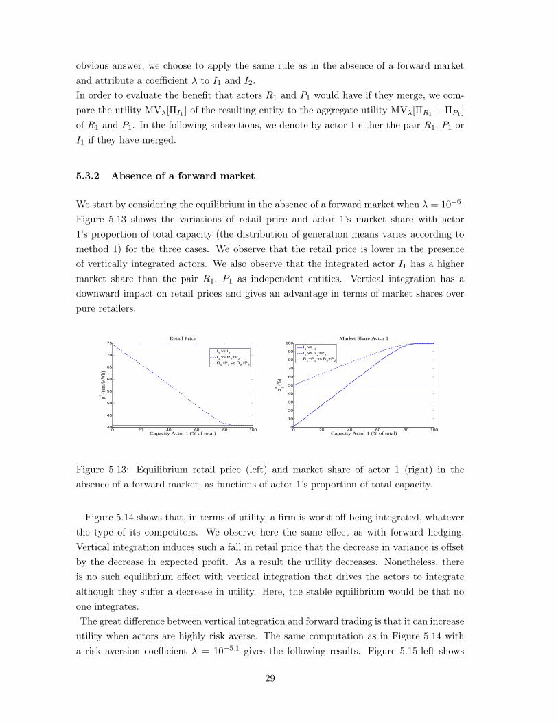
5.3.2 Absence of a forward market

We start by considering the equilibrium in the absence of a forward market when λ = 10−6.Figure 5.13 shows the variations of retail price and actor 1’s market share with actor1’s proportion of total capacity (the distribution of generation means varies according tomethod 1) for the three cases. We observe that the retail price is lower in the presenceof vertically integrated actors. We also observe that the integrated actor I1 has a highermarket share than the pair R1, P1 as independent entities. Vertical integration has adownward impact on retail prices and gives an advantage in terms of market shares overpure retailers.

0 20 40 60 80 10040

45

50

55

60

65

70

75Retail Price


p* (eur

o/M

Wh)

I1 vs I

2

I1 vs R

2+P

2

R1+P

1 vs R

2+P

2

0 20 40 60 80 1000

10

20

30

40

50

60

70

80

90

100Market Share Actor 1


α 1* (%)

I1 vs I

2

I1 vs R

2+P

2

R1+P

1 vs R

2+P

2

Figure 5.13: Equilibrium retail price (left) and market share of actor 1 (right) in theabsence of a forward market, as functions of actor 1’s proportion of total capacity.

Figure 5.14 shows that, in terms of utility, a firm is worst off being integrated, whateverthe type of its competitors. We observe here the same effect as with forward hedging.Vertical integration induces such a fall in retail price that the decrease in variance is offsetby the decrease in expected profit. As a result the utility decreases. Nonetheless, thereis no such equilibrium effect with vertical integration that drives the actors to integratealthough they suffer a decrease in utility. Here, the stable equilibrium would be that noone integrates.The great difference between vertical integration and forward trading is that it can increase

utility when actors are highly risk averse. The same computation as in Figure 5.14 witha risk aversion coefficient λ = 10−5.1 gives the following results. Figure 5.15-left shows

29

0 20 40 60 80 1000

0.5

1

1.5

2

2.5

3x 106 Utility Actor 1


U1 (e

uro)

I1 vs I

2

I1 vs R

2+P

2

R1+P

1 vs R

2+P

2

0 20 40 60 80 1000

0.5

1

1.5

2

2.5x 106 Utility Actor 2


U2 (e

uro)

I1 vs I

2I1 vs R

2+P

2R

1+P

1 vs R

2+P

2

Figure 5.14: Utility of actor 1 (left) and actor 2 (right) in the absence of a forward market,as functions of actor 1’s proportion of total capacity.

that, provided that R1 owns enough generation capacity, the utility of I1 facing R2 + P2

is higher than that of R1 + P1, hence an incentive to integrate in face of non-integratedactors. Similarly, figure 5.15-right shows that the utility of I2 facing I1 is always higherthan that of R2 + P2, hence an incentive to integrate in face of integrated actors. Thestable equilibrium in this case would be that all actors integrate.

0 20 40 60 80 100−10

−5

0



U1 (e

uro)

I1 vs I

2

I1 vs R

2+P

2

R1+P

1 vs R

2+P

2

0 20 40 60 80 100−10

−5

0



U2 (e

uro)

I1 vs I

2

I1 vs R

2+P

2

R1+P

1 vs R

2+P

2

Figure 5.15: Utility of actor 1 (left) and actor 2 (right) in the absence of a forward market,as functions of actor 1’s proportion of total capacity.

Conclusion. This case study shows that:- vertical integration has a downward impact on retail price- integrated producers can take larger market shares than pure suppliers- in terms of utility, actors with a low risk aversion are better off not integrating and

taking advantage of a higher retail price- in terms of utility, actors with a high risk aversion are better off integrating and

taking advantage of this natural hedge- vertical integration is a better risk diversification lever in the presence of highly risk

averse actors

30

5.3.3 Presence of a forward market

In the presence of a forward market and with risk aversion coefficient λ = 10−6, thebehaviour of retail price and market shares with respect to the actors’ total capacity issimilar as in the absence of it. Figure 5.16 shows the variation of these quantities withactor 1’s total capacity. We observe that vertical integration has a downward impact onretail prices, however this impact is smaller (at most 1 %) than in the previous case. Italso allows the integrated actor to gain higher market shares.

0 20 40 60 80 10040.55

40.6

40.65

40.7

40.75

40.8

40.85

40.9

40.95

41

41.05Retail Price


p* (eur

o/M

Wh)

I1 vs I

2

I1 vs R

2+P

2

R1+P

1 vs R

2+P

2

0 20 40 60 80 10010

20

30

40

50

60

70

80



α 1* (%)

I1 vs I

2

I1 vs R

2+P

2

R1+P

1 vs R

2+P

2

Figure 5.16: Equilibrium retail price (left) and market share of actor 1 (right) in thepresence of a forward market, as functions of actor 1’s proportion of total capacity.

Regarding utilities, Figure 5.17 shows that the impact of vertical integration is drasticallyreduced in the presence of a forward market. Being integrated or not almost leads to thesame utility. In addition, even for a larger risk aversion (ex: λ = 10−5.1), the incentive forvertical integration is reduced in the presence of a forward market.

0 20 40 60 80 1000

0.2

0.4

0.6

0.8

1

1.2

1.4

1.6

1.8



U1 (e

uro)

I1 vs I

2

I1 vs R

2+P

2

R1+P

1 vs R

2+P

2

0 20 40 60 80 1000

0.2

0.4

0.6

0.8

1

1.2

1.4

1.6

1.8



U2 (e

uro)

I1 vs I

2I1 vs R

2+P

2R

1+P

1 vs R

2+P

2

Figure 5.17: Utility of actor 1 (left) and actor 2 (right) in the presence of a forward market,as functions of actor 1’s proportion of total capacity.

Conclusion. This case study shows that:- the qualitative impact of vertical integration is not changed in the presence of a

31

forward market- the intensity of this impact is drastically reduced when forward contracts are available- the incentive to integrated is drastically reduced in the presence of a forward market

6 Extensions

6.1 Extension to the case of an elastic demand

In the previous sections the model was analyzed under the hypothesis of inelastic demand.If demand is elastic to spot price but we still assume perfect competition on the spot market,the results are unchanged because the spot market equilibrium remains independent ofretail and forward equilibrium. Nevertheless, if perfect competition is replaced by Cournotcompetition for example, the argument does not hold anymore and we are beyond thescope of our analysis.

As mentioned in Remark 2.1, the model can also be solved similarly in the presence ofdemand elasticity to retail price. Suppose that the demand is a random function of theretail price D(p). In this case, we can solve the equilibrium problem as in Sections 3 or4 and equations (3.5) and (4.1)-(4.2)-(4.3) remain valid. The only difference lies in theequation satisfied by p∗. In the presence of elasticity to retail prices, this equation reads:

0 = E[(p∗ − P ∗(p∗))D(p∗)]− 2ΛRCov[(p∗ − P ∗(p∗))D(p∗), (p∗ − P ∗(p∗))D(p∗) + ΠgI(p

∗)]

in the absence of a forward market, and:

0 = E[(p∗ − P ∗(p∗))D(p∗)]− 2ΛRCov[(p∗ − P ∗(p∗))D(p∗), (p∗ − P ∗(p∗))D(p∗) + ΠgI(p

∗)]

+2ΛRCov[P ∗(p∗), (p∗ − P ∗(p∗))D(p∗)]

Var[P ∗(p∗)]Cov

[P ∗(p∗), (p∗ − P ∗(p∗))D(p∗) + Πg

I(p∗)]

−2ΛCov[P ∗(p∗), (p∗ − P ∗(p∗))D(p∗)]

Var[P ∗(p∗)]Cov [P ∗(p∗), p∗D(p∗)− C(D(p∗))]

in the presence of it. This non-linear equation may be hard to solve, especially if we cannothave an explicit formulation of the spot equilibrium. Nevertheless, the equation simplifiesin some cases, as we show in the following subsection.

6.1.1 Particular case of quadratic cost functions

Consider the particular case of quadratic and symmetric cost functions:

ck(x) =c

2x2 , ∀k ∈ K .

Suppose in addition that demand is a linear function of retail price of the form:

D(p) = D0 − µ(p− p0) ,

32

where D0 is an exogenous random variable, p0 is some non-negative reference price andµ > 0. In this setting the equilibrium on the spot market can be solved explicitly and weobtain:

S∗k = 1

NPD(p∗), P ∗ = c

NPD(p∗)

Πgk = c

2N2P

D2(p∗), ΠgI = cNI

2N2P

D2(p∗)

Πg = c2NP

D2(p∗)

(6.1)

where NP is the number of producers and NI the number of integrated producers. Theretail price at equilibrium p∗ is then given by the smallest root of a second order polynomialequation (cf. Appendix A).

6.1.2 Examples

To illustrate the impact of demand elasticity, we compute the equilibrium found abovein two cases. First, we study the competition between one pure retailer and one pureproducer, as we did in paragraph 5.2.2. Second, we examine the case of a pure retailer andan integrated producer, as in paragraph 5.2.1. To this end, we use the demand samples ofthe previous section. Taking expectation on both sides of the equation giving P ∗ in (6.1),we estimate the cost function coefficient c as:

c = NPE[P ∗]E[D]

' NP × 5.6143 10−4 .

We set p0 = E[P ] ' 37.95 as the expected spot price, and we express the elasticitycoefficient µ in percentage of expected demand E[D].Pure retailer and pure producer. In this case, actor 1 is the pure producer and actor2 the pure retailer. We set both risk aversion coefficients to λ1 = λ2 = 10−6. Figure 6.18-right shows the equilibrium retail price in the absence and presence of a forward market,as a function of µ, in percentage of E[D]. We still observe that the presence of a forward

0 10 20 30 40 506.2

6.3

6.4

6.5

6.6

6.7

6.8x 104 Expected Demand

µ (%)

E[D

* ] (M

Wh)

Without FW MarketWith FW Market

0 10 20 30 40 5037.5

38

38.5

39

39.5

40

40.5

41Retail Price

µ (%)

p* (eur

o/M

Wh)


Figure 6.18: Expected demand (left) and retail price (right) at equilibrium in the absenceand presence of a forward market as a function of µ.

33

market has a downward impact on retail price. Nonetheless, this impact tends to shrink asdemand elasticity increases. We also note that, in both cases, demand elasticity decreasesthe retail price. As customers respond to retail price, the retailers face low demand if theyset a high retail price. They are thus forced to decrease the equilibrium retail price.

0 10 20 30 40 501.04

1.06

1.08

1.1

1.12

1.14

1.16

1.18

1.2


µ (%)

U1

(eur

o)

0 10 20 30 40 501.26

1.265

1.27

1.275

1.28

1.285

1.29

1.295


µ (%)

U1

(eur

o)Figure 6.19: Actor 1’s utility in the absence (left) and presence (right) of a forward marketas a function of µ.

Figure 6.19 shows actor 1’s utility with and without a forward market. We still ob-serve that this utility increases in the presence of a forward market, but the interestingaspect here is that the pure producer’s utility decreases with demand elasticity. We al-ready mentioned the strong asymmetry between retailers and producers: producers setthe equilibrium spot price and thus impact retailers’ profit, while retailers cannot impactproducers’ profit. When demand is elastic to retail price, this asymmetry is reduced andretailers impact producers’ profit via the retail price. Since the expected demand decreaseswith demand elasticity (see Figure 6.18-left), so does the producers’ utility.

Concerning actor 2, we observe on figure 6.20 that its utility decreases with demand

0 10 20 30 40 507

7.2

7.4

7.6

7.8

8


µ (%)

U2

(eur

o)

0 10 20 30 40 502269.36

2269.38

2269.4

2269.42

2269.44

2269.46

2269.48

2269.5

2269.52

2269.54Utility Actor 2

µ (%)

U2

(eur

o)

Figure 6.20: Actor 2’s utility in the absence (left) and presence (right) of a forward marketas a function of µ.

elasticity in the absence of a forward market but increases in its presence. In the absenceof a forward market, the pure retailer is impacted by both the decrease in demand and

34

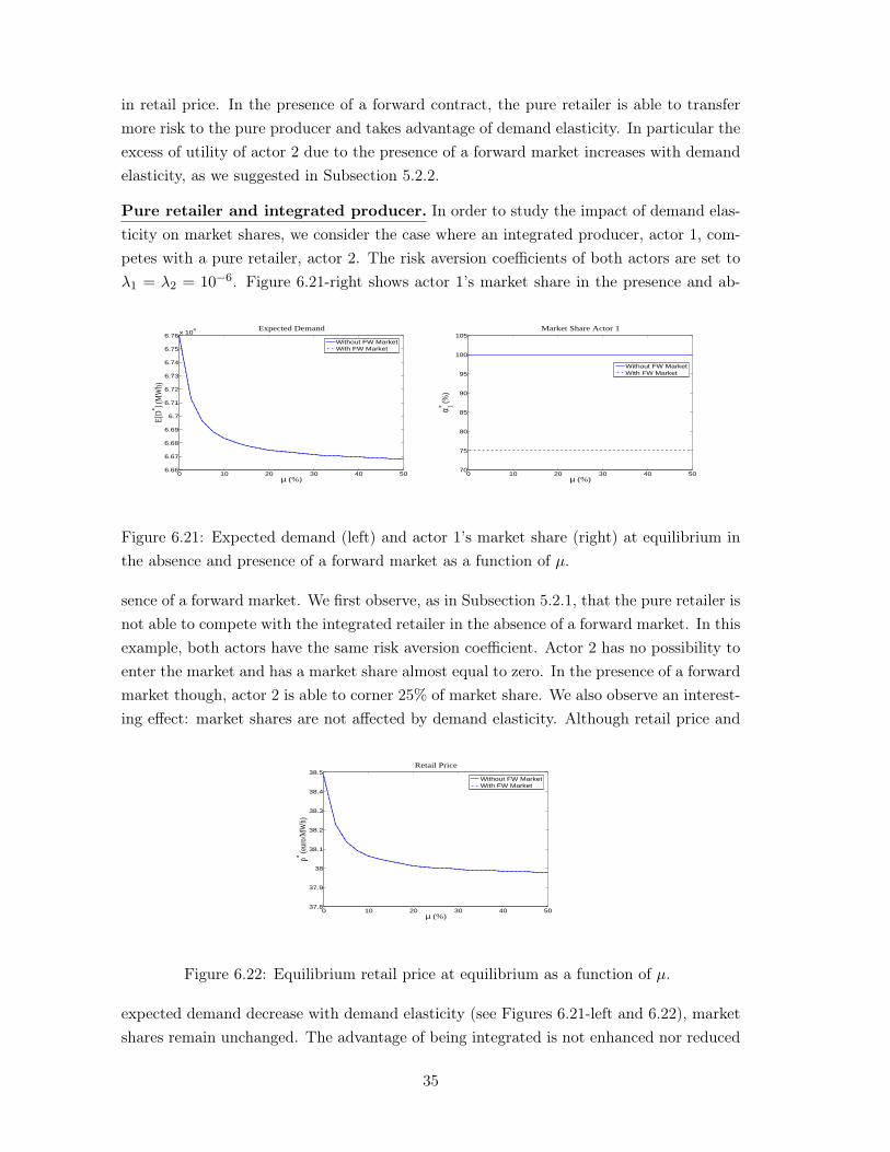
in retail price. In the presence of a forward contract, the pure retailer is able to transfermore risk to the pure producer and takes advantage of demand elasticity. In particular theexcess of utility of actor 2 due to the presence of a forward market increases with demandelasticity, as we suggested in Subsection 5.2.2.

Pure retailer and integrated producer. In order to study the impact of demand elas-ticity on market shares, we consider the case where an integrated producer, actor 1, com-petes with a pure retailer, actor 2. The risk aversion coefficients of both actors are set toλ1 = λ2 = 10−6. Figure 6.21-right shows actor 1’s market share in the presence and ab-

0 10 20 30 40 506.66

6.67

6.68

6.69

6.7

6.71

6.72

6.73

6.74

6.75

6.76x 104 Expected Demand

µ (%)

E[D

* ] (M

Wh)


0 10 20 30 40 5070

75

80

85

90

95

100


µ (%)

α 1* (%)


Figure 6.21: Expected demand (left) and actor 1’s market share (right) at equilibrium inthe absence and presence of a forward market as a function of µ.

sence of a forward market. We first observe, as in Subsection 5.2.1, that the pure retailer isnot able to compete with the integrated retailer in the absence of a forward market. In thisexample, both actors have the same risk aversion coefficient. Actor 2 has no possibility toenter the market and has a market share almost equal to zero. In the presence of a forwardmarket though, actor 2 is able to corner 25% of market share. We also observe an interest-ing effect: market shares are not affected by demand elasticity. Although retail price and

0 10 20 30 40 5037.8

37.9

38

38.1

38.2

38.3

38.4

38.5Retail Price

µ (%)

p* (eur

o/M

Wh)


Figure 6.22: Equilibrium retail price at equilibrium as a function of µ.

expected demand decrease with demand elasticity (see Figures 6.21-left and 6.22), marketshares remain unchanged. The advantage of being integrated is not enhanced nor reduced

35

in the presence of demand elasticity.

Conclusion. The results presented above show that the assumption of demand inelasticityto retail price, assumed in the previous sections, is not restrictive regarding our objective.Our conclusions concerning the impact of vertical integration and forward trading on riskdiversification remain unchanged in the presence of demand elasticity to retail price.

6.2 Other definitions of an equilibrium

In our analysis, the equilibrium was defined in Definition 2.1 as a simultaneous equilib-rium on both the retail and forward markets. The following two definitions can also beconsidered, that introduce a sequentiality between the two markets. We use the followingnotation: (α∗

−k, αk) := (α∗1, . . . , α

∗k−1, αk, α

∗k+1, . . . , α

∗|R|).

Definition 6.1. A sequential equilibrium with anticipation of the forward positions is aquadruple (p∗, q∗, α∗, f∗) ∈ R+×R+×A×F, such that there exist two functions q : A 7→ Rand f : A 7→ F verifying

fk(α) = argmaxfk

MVλk[Πk (p∗, q(α), αk, fk)] , ∀k ∈ K (6.2)

α∗k = argmax

αk

MVλk

[Πk

(p∗, q(α∗

−k, αk), αk, fk(α∗−k, αk)

)], ∀k ∈ K (6.3)

q∗ = q(α∗) (6.4)

f∗ = f(α∗) (6.5)

This equilibrium corresponds to a two-step equilibrium where the actors first decide theirmarket shares. Define the set

A :=

(αk)k∈K ∈ R|K| : ∀k /∈ S, αk = 0 and

∑k∈K

αk = 1

,

this following definition describes the situation where the actors first invest on the forwardmarket before deciding their market shares:

Definition 6.2. A sequential equilibrium with anticipation of the market shares is aquadruple (p∗, q∗, α∗, f∗) ∈ R+×R+×A×F, such that there exist two functions p : F 7→ Rand α : F 7→ A verifying

αk(f) = argmaxαk

MVλk[Πk(p(f), q∗, αk, fk)] , ∀k ∈ K (6.6)

f∗k = argmaxfk

MVλk

[Πk

(p(f∗−k, fk), q∗, αk(f∗−k, fk), fk

)], ∀k ∈ K (6.7)

p∗ = p(f∗) (6.8)

α∗ = α(f∗) (6.9)

36

We can in fact prove that the above two definitions are equivalent to Definition 2.3. Thisis done by deriving explicitly the expression of the equilibrium in each case and showingthat the equilibrium prices and positions are exactly the same as in Proposition 4.1. It isprobable that this equivalence result disappears when the markets are no longer assumedcompetitive.

7 Conclusion

We developed a competitive equilibrium model for retail, forward and spot markets of anon-storable good. Our aim was to understand the fundamental mechanisms of risk diver-sification in this kind of economy. We stated the explicit formulation of the equilibriumprices and positions on each market. Finally, we illustrated the model with case studies inthe electricity sector.We showed that vertical integration and forward hedging are two levers for achieving riskdiversification, that exhibit similar properties. First, they both have a downward impacton retail price. Second, they both allow for actors with low generation capacity to cornerlarger market shares. Third, they both tend to decrease downstream firms’ utility whenupstream firms are only partially integrated. Fourth, the impact of one of these levers oneretail price and utilities is drastically reduced in the presence of the other.We also showed that they exhibit discrepancies because of the asymmetric structure of riskbetween upstream and downstream. First, we showed that vertical integration restoresthis symmetry while forward hedging does not. Second, vertical integration is more robusttowards high risk aversions in the sense that it can achieve risk diversification when forwardhedging fails. Third, vertical integration can also increase downstream firms’ utility pro-vided that they have sufficiently high risk aversion. Fourth, a non-integrated economy canbe a stable equilibrium whereas actors always trade forward contract at equilibrium whenthey are available. Finally, we proved that these conclusions still prevail in the presence ofdemand elasticity to retail price.Our main conclusion is that vertical integration has a positive impact, especially in termsof lower retail prices. In terms of risk diversification, it exhibits properties that linearinstruments such as forward contracts can not achieve. It finally helps reducing the asym-metric risk structure between upstream and downstream. We then converge to the ideaof Chao, Oren and Wilson that some level of integration is benefic even in the presence ofwholesale markets. Nonetheless, our approach does not take into account the impact ofmarket power that such large actors can exercise. Allaz showed in [1] the implications offorward trading on producers’ market power. Vertical integration seems to have a differentimpact. It would be interesting to study the resulting impact when these two factors coex-ist. Future developments in the field of electricity market equilibria should integrate thoseelements into the risk management analysis. Our analysis could then serve as a benchmark

37

to measure the effects of imperfect competition.

A Appendix

Proof of Proposition 3.1Maximizing the mean-variance criteria over αk yields the following first order condition for actork ∈ R:

0 = E[(p∗ − P ∗)D]− 2λkCov[(p∗ − P ∗)D, (p∗ − P ∗)α∗kD + Πgk] ,

which is sufficient for maximality by convexity, and gives:

α∗k =E[(p∗ − P ∗)D]

2λkVar[(p∗ − P ∗)D]−

Cov[(p∗ − P ∗)D,Πgk]

Var[(p∗ − P ∗)D].

The coupling constraint∑

k∈R α∗k = 1 gives the condition on p∗:

0 = E[(p∗ − P ∗)D]− 2ΛRVar[(p∗ − P ∗)D]− 2ΛRCov[(p∗ − P ∗)D,ΠgI ] ,

and allows us to derive (3.6).

Proof of Proposition 4.1If k ∈ R, the first order condition of profit maximization reads:

0 = M

[f∗kα∗k

]−

[E[P∗−q∗]

2λk− Cov[P ∗,Πg

k]E[(p∗−P∗)D]

2λk− Cov[(p∗ − P ∗)D,Πg

k]

],

where M is the variance-covariance matrix of vector [P ∗, (p∗ − P ∗)D]. By inverting the system,we obtain the expressions of f∗k and α∗k in terms of p∗ and q∗. If k /∈ R, Πk does not depend onαk and the first order condition reads:

0 = E[P ∗ − q∗]− 2λkCov[P ∗ − q∗, (P ∗ − q∗)f∗k + Πgk] .

Market-clearing constraint (2.2) can be expressed as:

0 =∑k∈K

f∗k

=Var[(p∗ − P ∗)D]

∆

(E[P ∗ − q∗]

2ΛR− Cov[P ∗,

∑k∈R

Πgk]

)

−Cov[P ∗, (p∗ − P ∗)D]∆

(E[(p∗ − P ∗)D]

2ΛR− Cov[(p∗ − P ∗)D,

∑k∈R

Πgk]

)

+E[P ∗ − q∗]2Var[P ∗]

(1Λ− 1

ΛR

)−

Cov[P ∗,∑KR Πg

k]Var[P ∗]

,

where ∆ is in fact the determinant of M , which leads to:

0 = ∆

(E[P ∗ − q∗]

2Λ− Cov[P ∗,

∑k∈K

Πgk]

)(A.1)

−Cov[P ∗, (p∗ − P ∗)D]Var[P ∗]

(E[(p∗ − P ∗)D]

2ΛR− Cov[(p∗ − P ∗)D,

∑k∈R

Πgk]

)

+Cov2[P ∗, (p∗ − P ∗)D]

(E[P ∗ − q∗]

2ΛR− Cov[P ∗,

∑k∈R

Πgk]

).

38

Load satisfaction constraint (2.1) reads:

1 =∑k∈R

α∗k

= −Cov[P ∗, (p∗ − P ∗)D]∆

(E[P ∗ − q∗]

2ΛR− Cov[P ∗,

∑k∈R

Πgk]

)

+Var[P ∗]

∆

(E[(p∗ − P ∗)D]

2ΛR− Cov[(p∗ − P ∗)D,

∑k∈R

Πgk]

),

which yields, using (A.1):

0 =E[P ∗ − q∗]

2Λ− Cov[P ∗, (p∗ − P ∗)D +

∑k∈K

Πgk] .

As∑

k∈KΠgk = P ∗D − C(D), we obtain equation (4.3). Using this result to simplify (A.1), we

derive the desired expression (4.4) for p∗. Finally, using those two equations, we can re-arrangethe expressions for f∗k and α∗k to obtain equations (4.1) and (4.2).

Equations for the retail price under elastic demandThe retail price at equilibrium p∗ is then given by the smallest root of the second order polynomial:

0 = (p∗)2−µ

(1 + µ

c

NP

)− 2ΛR

[1 + 4µ

c

NP

(1 + µ

c

NP

)− µ

c

NP

NI

NP

(1 + 2µ

c

NP

)]Var[D0]

+p∗

(1 + 2µ

c

NP

)E[D0] + µp0

(1 + 2µ

c

NP

)+p∗ΛR

c

NP

(4− NI

NP+ 4µ

c

NP

(2− NI

NP

))(Cov[D0, D

20] + 2µp0Var[D0]

)− c

NP

(E[D2

0] + 2µp0E[D0] + µ2p20

)−ΛR

c2

N2P

(2− NI

NP

)(Var[D2

0] + 4µp0Cov[D0, D20] + 4µ2p2

0Var[D0])

in the absence of a forward market, and by:

0 = (p∗)2−µ− µ2 c

NP− 2Λ

(1 + 3µ

c

NP+ 2µ2 c2

N2P

)Var[D0]

+p∗

(1 + 2µ

c

NP

)E[D0] + µp0

(1 + 2µ

c

NP

)+p∗Λ

c

NP

(3 + 4µ

c

NP

)(Cov[D0, D

20] + 2µp0Var[D0]

)− c

NP

(E[D2

0] + 2µp0E[D0] + µ2p20

)− ΛR

c2

N2P

(2− NI

NP

)Var[D2

0]

+2ΛRc2

N2P

(1− Λ

2ΛR− NI

2NP

)Cov2[D0, D

20]

Var[D0]

−4µp0Λc2

N2P

(Cov[D0, D

20] + µp0Var[D0]

)in the presence of a forward market.

39

References

[1] B. Allaz, Oligopoly, uncertainty and strategic forward transactions, International Jour-nal of Industrial Organization (1992), no. 10, 297–308.

[2] B. Allaz and Vila J.L., Cournot competition, forward markets and efficiency, Journalof Economic Theory 59 (1993), no. 1, 1–16.

[3] K.J. Arrow, Vertical integration and communication, Bell Journal of Economics(1975), no. 6, 175–183.

[4] H. Bessembinder and M.L. Lemmon, Equilibrium pricing and optimal hedging in elec-tricity forward markets, The Journal of Finance LVII (2002), no. 3, 1347–1382.

[5] P. Bolton and M.D. Whinston, Incomplete contracts, vertical integration and supplyassurance, The Review of Economic Studies 60 (1993), no. 1, 121–148.

[6] D.W. Carlton, Vertical integration in competitive markets under uncertainty, TheJournal of Industrial Economics 27 (1979), no. 3, 189–209.

[7] H. Chao, S. Oren, and R. Wilson, Restructured electricity markets: A risk managementapproach, Tech. report, EPRI Technical Paper, July 2005.

[8] , Restructured electricity markets: Reevaluation of vertical integration and un-bundling, Tech. report, EPRI Technical Paper, July 2005.

[9] W Emons, Good times, bad times, and vertical upstream integration, InternationalJournal of Industrial Organization 14 (1996), 465–484.

[10] C. Gollier, The economics of risk and time, MIT Press, Cambridge, MA, 2004.

[11] J.K. Green, New developments in the analysis of market structure, MIT Press, Cam-bridge, 1986, Vertical Integration and Assurance of Markets.

[12] G. Hendrikse and H. Peters, A note on partial vertical integration, Economics Letters(1989), no. 30, 249–252.

[13] P. Joskow, Handbook of new institutional economics, Kluwer Academic Publishing,2003, Vertical Integration.

[14] P.L. Joskow, Vertical integration and long-term contracts: The case of coal-burningelectric generating plants, Journal of Law 1 (1985), no. 1, 33–80.

[15] B. Klein, Vertical integration as organizational ownership: The fisher body-generalmotors relationship revisited, Journal of Law 4 (1988), no. 1, 199–213.

[16] H.M. Markowitz, Approximating expected utility by a function of mean and variance,American Economic Review (1979), no. 69, 308–317.

40

[17] M.K. Perry, Handbook of industrial organization, Elsevier, 1989, Vertical Integration:Determinants and Effects.

[18] O.E. Williamson, The vertical integration of production: Market failure considerations,The American Economic Review 61 (1971), no. 2, 112–123.

[19] R. Wilson, The theory of syndicates, Econometrica 36 (1968), no. 1, 119–132.

41

vertical integration and risk management in competitive

Documents