vertex-centred discretization of multiphase compositional...

ECMOR XIII – 13th European Conference on the Mathematics of Oil Recovery Biarritz, France, 10-13 September 2012

B17Vertex-centred Discretization of MultiphaseCompositional Darcy Flows on General MeshesR. Eymard (University Paris East), C. Guichard* (University of Nice SophiaAntipolis), R. Herbin (University of Provence), R. Masson (University ofNice Sophia Antipolis) & P. Samier (Total)

SUMMARYThis paper introduces a vertex centred discretization on general 3D meshes of multiphase Darcy flows inheterogeneous anisotropic porous media.The model accounts for the coupling of the mass balance of each component with the pore volumeconservation and the thermodynamical equilibrium.The conservative spatial discretization of the Darcy fluxes is based on the Vertex Approximate Gradientscheme (VAG) which is unconditionally coercive for arbitrary meshes and permeability tensors.The stencil of this vertex-centred scheme typically comprises 27 points on topologically Cartesian meshes.On tetrahedral meshes, the number of unknowns is considerably reduced, by typically a factor five,compared with usual cell-centred MultiPoint Fluxes Approximations, which is a key asset for multiphaseflow simulations on unstructured meshes.An adaptive choice of the pore volume at the vertices ensures the accuracy of the discretization even forcoarse meshes on highly heterogeneous media.This approach can easily be implemented on existing reservoir simulators using a graph oftransmissibilities for the computation of the fluxes.The efficiency of our approach is exhibited on several two phase and three phase Darcy flow examples. Inparticular it includes the nearwell injection of miscible CO2 in a saline aquifer taking into account theprecipitation of salt.

Introduction

Many applications require the simulation of compositional multiphase Darcy flow in heterogeneousporous media. In oil reservoir modelling, the compositional triphase Darcy flow simulator is a key toolto predict and optimize the production of a reservoir. In sedimentary basin modelling, such models areused to simulate the migration of the oil and gas phases in a basin saturated with water at geologicalspace and time scales. The objectives are to predict the location of the potential reservoirs as well as thequality and quantity of oil trapped therein. In CO2 geological storage, compositional multiphase Darcyflow models are used to optimize the injection of CO2 and to assess the long term integrity of the storage.The numerical simulation of such models is a complex task, which has been the object of several worksover a long period of time, see the reference books [7] and [21]. Several types of numerical schemeshave been proposed in the past decades. Those which are implemented in industrial codes are mainlybuilt upon cell centred approximations and discrete fluxes, in a framework which is also that of themethod we propose here. Let us briefly sketch this framework.

The 3D simulation domain Ω is meshed by control volumes X ∈ G . Let us denote by Λ the diffusionmatrix (which is a possibly full matrix depending on the point of the domain). For each control volumeX ∈ G , the set of neighbours Y ∈NX is the set of all control volumes involved in the mass balance in X ,which means that the following approximation formula is used:

−∫

Xdiv(Λ∇p)dx ' ∑

Y∈NX

FX ,Y (P),

where P = (pZ)Z∈G is the family of all pressure unknowns in the control volumes, and where the fluxFX ,Y (P), between control volumes X and Y , is a linear function of the components of P which ensuresthe following conservativity property:

FX ,Y (P) =−FY,X(P). (1)

Such a linear function, which is expected to vanish on constant families, may be defined by

FX ,Y (P) = ∑Z∈GX ,Y

aZX ,Y pZ, (2)

where the family (aZX ,Y )Z∈GX ,Y and GX ,Y ⊂ G are such that ∑Z∈GX ,Y aZ

X ,Y = 0. We then consider a compo-sitional multiphase Darcy flow, with Nα phases and Nc constituents, the discrete balance law in X ∈ Gis written

ΦX

δt(A(n+1)

X ,i −A(n)X ,i)+

Nα

∑α=1

∑Y∈NX

M(n+1),αX ,Y,i F(n+1),α

X ,Y = 0, ∀i = 1, . . . ,Nc,

F(n+1),αX ,Y = FX ,Y (P(n+1),α)−ρ

(n+1),αX ,Y g · (xY − xX), ∀α = 1, . . . ,Nα ,

(3)

where n is the time index, δt is the time step, ΦX is the porous volume of the control volume X , AX ,i

represents the accumulation of constituent i in the control volume X per unit pore volume (assumedto take into account the dependence of the porosity with respect to the pressure), Mα

X ,Y,i is the amountof constituent i transported by phase α from the control volume X to the control volume Y (generallycomputed by taking the upstream value with respect to the sign of Fα

X ,Y ), Pα is the family of the pressureunknowns of phase α , g is the gravity acceleration, ρα

X ,Y is the bulk density of phase α between controlvolumes X and Y and xX is the centre of control volume X . In addition to these relations, the differencesbetween the phase pressures are ruled by capillary pressure laws. Thermodynamical equilibrium andstandard closure relations are used. A more detailed description of this model is described, for examplein [17].

The main drawback of cell-centred finite volume schemes is the difficulty to use them in the case ofcomplex meshes and heterogeneous anisotropic permeabilities, which are unfortunately frequently en-countered in practice to represent the basin and reservoir geometries and petrophysical properties. Many

ECMOR XIII – 13th European Conference on the Mathematics of Oil RecoveryBiarritz, France, 10-13 September 2012

progresses have been done during the last decade, leading to the design of cell-centred schemes whichremain consistent in such situations. Among these, let us mention for example the well-known O schemeintroduced in [1, 2, 10, 11], the L scheme [3], or the SUSHI scheme [14]. We also refer to [4, 5, 6] for theconvergence analysis of cell-centred schemes in a general framework. Nevertheless it is still a challengeto design a cell-centred discretization of diffusive fluxes in the case of general meshes and heterogeneousanisotropic diffusion tensors, which is linear, unconditionally coercive and “compact”, in the sense thatthe expression of the discrete flux at a given face of the mesh may at most involve the cells sharing avertex with this face. For example the O and L schemes are compact but their coercivity is mesh andpermeability tensor dependent. On the other hand, the SUSHI scheme is unconditionally coercive butits stencil is not compact, since it involves the neighbours of the neighbours of a given control volume.

Alternately to cell centred schemes, vertex centred schemes, such as the CVFE (Control Volume FiniteElement, see for example [12, 9, 20]), are more adapted to unstructured meshes such as tetrahedralmeshes and can lead in some cases to coercive schemes. The main difficulty of vertex centred schemeslies in the definition of the rock properties in the case of heterogeneous media. Indeed, assuming thatthe control volumes are vertex centred with vertices located at the interfaces between different media,then the porous volume concerned by the flow of very permeable medium includes that of non perme-able medium. This may lead to surprisingly wrong results on the components velocities. A possibleinterpretation of these poor results is that, when seen as a set of discrete balance laws, the finite ele-ment discretization provides the same amount of impermeable and permeable porous volume for theaccumulation term for a node located at a heterogeneous interface.

We present in this paper the use of a new scheme, called Vertex Approximate Gradient (VAG) scheme[15, 16] which try to overcome the above difficulties. The key idea is to use both cell and vertexunknowns in order to obtain and unconditionally coercive scheme on general polyhedral meshes. TheVAG scheme can be implemented in (3) so that the components velocities are correctly approximated,thanks to a special choice of the control volumes and of the discrete fluxes, which respect the form(2). The purpose of respecting the form (1)-(3) is to be able to easily plug it into an existing reservoircode, say Multi-Point Flux Approximation (MPFA), by simply redefining the control volumes and thecoefficients aZ

X ,Y of the discrete flux. Although this scheme is mainly vertex centred, we show that thesolution obtained on a very heterogeneous medium with a coarse mesh remains accurate. This is a greatadvantage of this scheme, which is also consistent, unconditionally coercive, symmetric, and leads to a27-stencil on hexahedral structured meshes since the cell unknowns can be eliminated locally withoutany fill-in. In addition the VAG scheme is very efficient, in terms of CPU time, on meshes with tetrahedraas illustrated in the numerical examples.

The outline of the paper is the following. Section one recalls the construction of the VAG scheme fordiffusive equations. Then, the VAG scheme fluxes are derived and used in to discretize the compositionalmultiphase Darcy flow model (3), and the pore volume assignment procedure is detailed. Finally, thesecond section exhibits the efficiency of the VAG discretization which is compared to the solutionsobtained with the MPFA O scheme. The first test cases deal with two phase flow examples includinghighly heterogeneous cases and discontinuous capillary pressures. Then, the last test case considers thenearwell injection of miscible CO2 in a saline aquifer, taking into account the vaporization of H2O inthe gas phase as well as the precipitation of salt.

Presentation of the VAG scheme

Recently, a new discretization of diffusive equations, the Vertex Approximate Gradient (VAG) schemehas been introduced in [15, 16]. In addition to its properties listed in the introduction, it is exact oncellwise affine solutions for cellwise constant diffusion tensors. Moreover it has exhibited a very goodcompromise between accuracy, robustness and CPU time in the recent FVCA6 3D benchmark [19].Thus its use for compositional multiphase Darcy flow model (3) was a natural question to study and for


which an answer is given in the following section.

We consider the following diffusion equation,−div(Λ∇u) = f in Ω,

u = uD on ∂Ω,

and its variational formulation: which reads find u ∈ H1(Ω) such that u = uD on ∂Ω, and∫Ω

Λ∇u ·∇v dx =∫

Ω

f v dx

for all v ∈ H10 (Ω) = w ∈ H1(Ω) |w = 0 on ∂Ω, admits a unique solution u provided that the measure

of ∂Ω is nonzero, that f ∈ L2(Ω) and uD ∈ H1/2(∂Ω), which is assumed in the following. Note thatthe case of inhomogeneous Neumann boundary condition is detailed for example in [18, 17] and notdetailed here for sake of simplicity.

Discrete framework of the VAG scheme

Following [16], we consider M a general polyhedral mesh of Ω defined by a set of cells K that aredisjoint open subsets of Ω such that

⋃K∈M K = Ω. For all K ∈M , xK denotes the so-called “centre” of

the cell K under the assumption that K is star-shaped with respect to xK . Let F denote the set of facesof the mesh which are not assumed to be planar, hence the term “generalized polyhedral cells”. Wedenote by V the set of vertices of the mesh. Let VK , FK , Vσ respectively denote the set of the verticesof K ∈M , faces of K, and vertices of σ ∈F . For any face σ ∈FK , we have Vσ ⊂ VK . Let Ms denotethe set of the cells sharing the vertex s. The set of edges of the mesh is denoted by E and Eσ denotes theset of edges of the face σ ∈F . It is assumed that, for each face σ ∈F , there exists a so-called “centre”of the face xσ such that

xσ = ∑s∈Vσ

βσ ,s s, with ∑s∈Vσ

βσ ,s = 1,

where βσ ,s≥ 0 for all s∈Vσ . The face σ is assumed to match with the union of the triangles Tσ ,e definedby the face centre xσ and each of its edge e ∈ Eσ . Let Vint = V \∂Ω denote the set of interior vertices,and Vext = V ∩∂Ω the set of boundary vertices.

The previous discretization is denoted by D and we define the discrete space

WD = vK ∈ R,vs ∈ R, for K ∈M and s ∈ V ,

and its subspace with homogeneous Dirichlet boundary conditions on Vext

WD = v ∈ WD |vs = 0 for s ∈ Vext.

The VAG scheme introduced in [16] is based on a piecewise constant discrete gradient reconstruction forfunctions in the space WD. Several constructions are proposed based on different decompositions of thecell. Let us recall the simplest one based on a conforming finite element discretization on a tetrahedralsub-mesh, and we refer to [16, 15] for two other constructions sharing the same basic features.

For all σ ∈F , the operator Iσ : WD→ R such that

Iσ (v) = ∑s∈Vσ

βσ ,svs,

is by definition of xσ a second order interpolation operator at point xσ .

Let us introduce the tetrahedral sub-mesh

T = TK,σ ,e for e ∈ Eσ ,σ ∈FK ,K ∈M


xσ

s

xKe

s′

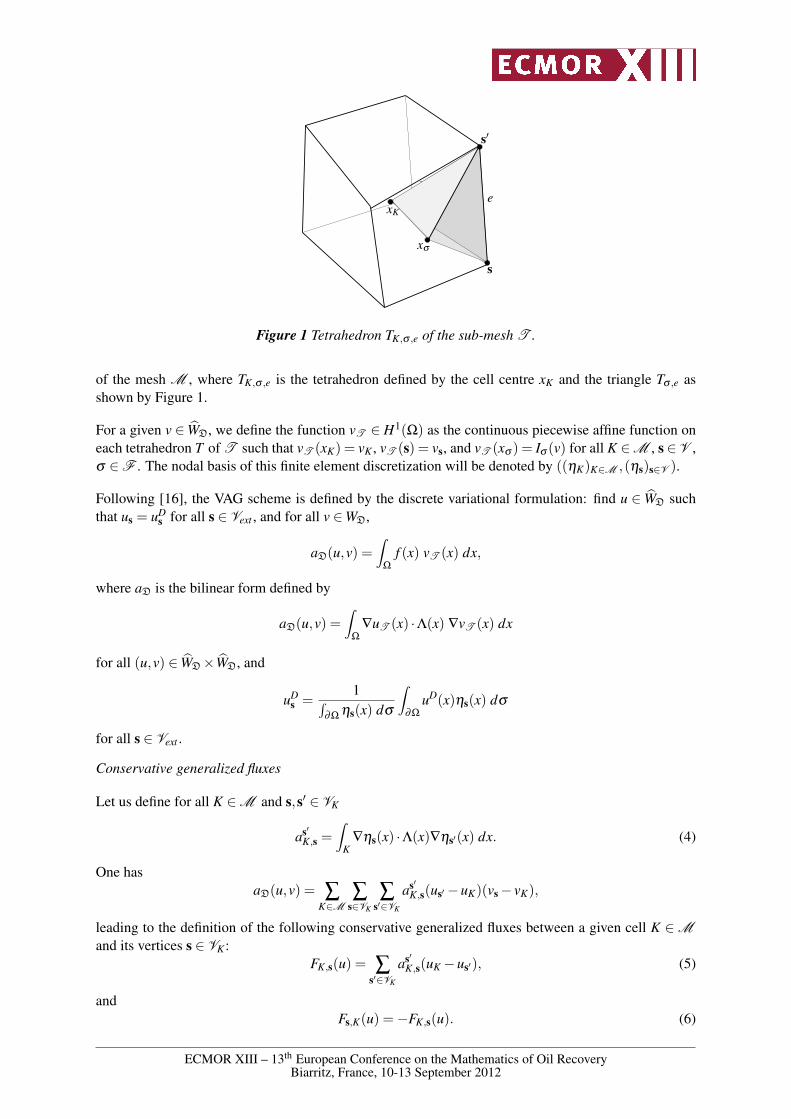
Figure 1 Tetrahedron TK,σ ,e of the sub-mesh T .

of the mesh M , where TK,σ ,e is the tetrahedron defined by the cell centre xK and the triangle Tσ ,e asshown by Figure 1.

For a given v ∈ WD, we define the function vT ∈ H1(Ω) as the continuous piecewise affine function oneach tetrahedron T of T such that vT (xK) = vK , vT (s) = vs, and vT (xσ ) = Iσ (v) for all K ∈M , s ∈ V ,σ ∈F . The nodal basis of this finite element discretization will be denoted by ((ηK)K∈M ,(ηs)s∈V ).

Following [16], the VAG scheme is defined by the discrete variational formulation: find u ∈ WD suchthat us = uD

s for all s ∈ Vext , and for all v ∈WD,

aD(u,v) =∫

Ω

f (x) vT (x) dx,

where aD is the bilinear form defined by

aD(u,v) =∫

Ω

∇uT (x) ·Λ(x) ∇vT (x) dx

for all (u,v) ∈ WD×WD, and

uDs =

1∫∂Ω

ηs(x) dσ

∫∂Ω

uD(x)ηs(x) dσ

for all s ∈ Vext .

Conservative generalized fluxes

Let us define for all K ∈M and s,s′ ∈ VK

as′K,s =

∫K

∇ηs(x) ·Λ(x)∇ηs′(x) dx. (4)

One hasaD(u,v) = ∑

K∈M∑

s∈VK

∑s′∈VK

as′K,s(us′−uK)(vs− vK),

leading to the definition of the following conservative generalized fluxes between a given cell K ∈Mand its vertices s ∈ VK :

FK,s(u) = ∑s′∈VK

as′K,s(uK−us′), (5)

andFs,K(u) =−FK,s(u). (6)


The VAG scheme is equivalent to the following discrete system of balance equations:

∑s∈VK

FK,s(u) =∫

Kf (x) ηK(x) dx, K ∈M ,

∑K∈Ms

Fs,K(u) =∫

Ω

f (x) ηs(x) dx, s ∈ Vint ,

us = uDs , s ∈ Vext .

Let us notice, that the first equation in the above system involves for each cell K the only cell unknownuK . It results that the cell unknowns can be eliminated of the above system without any fill-in leading toa vertex centred scheme with typically a 27 points stencil on topologically Cartesian grids.

One may easily check that the VAG scheme generalized fluxes can be rewritten as follows:

FK,s(u) =∫

K−Λ(x)∇uT (x) ·∇ηs(x) dx. (7)

This formula provides in 2D an interpretation of the VAG scheme generalized fluxes as Control VolumeFinite Element (CVFE) fluxes [9] on a triangular submesh. In 2D, xσ is chosen to be the mid-point of

the edge σ = ss′, and the interpolation is simply defined by Iσ (v) =vs + vs′

2. It results that the triangular

submesh T is rather defined in 2D as the set of triangles obtained for each cell K by joining each faceσ of the cell K to the cell centre xK . Then, the VAG scheme reduces to the P1 finite element scheme onthe submesh T . Let a be the mid-point of sxK (see figure 2). Using (7), one easily shows that, assuminga cellwise constant tensor field Λ, one has

FK,s(u) =∫

_xσ a∪ _

xσ ′a−Λ(x)∇uT (x) ·nKdσ ,

where_

xσ a (respectively_

xσ ′a) is any curved segment inside the triangle σxK (respectively σ ′xK) andnK is the normal outward the CVFE control volume containing xK (see figure 2). The flexibility in thedefinition of the curved edges of the CVFE control volumes will be exploited in the next subsection toadapt the porous volume at the vertices and at the cell centres of the mesh in heterogeneous cases. This

s

s′ s′′

xσxσ ′

axK

nxKs′ nxKs′′

Figure 2 CVFE interpretation of the fluxes FK,s(u) in the 2D case.

geometrical CVFE interpretation of the VAG generalized fluxes cannot be extended to the 3D case dueto the interpolation at the face centres which has been used to avoid numerous additional unknowns atthe faces.


Application to a compositional multiphase Darcy flow model

This subsection presents how to use the VAG scheme fluxes to discretize a compositional multiphaseDarcy flow on a general mesh, following the framework described in the introduction by (1)-(3). Due tothe previous definition of the VAG fluxes (5)-(6), the first idea is to define the set of control volumes Gas the union of the cells and of the interior vertices

G = M ∪Vint .

Remark that G must also include Neumann boundary vertices if this boundary condition is used in theproblem, see [17]. Thus the flux from control volume X = K to control volume Y = s is then given by

FX ,Y (u) = FK,s(u) , ∀s ∈ VK

and satisfies a MPFA formulation (1)-(2) due to (5) and (6). These generalized fluxes FK,s(u), betweena cell K and its vertices s ∈ VK , are then classically used for the approximation of the transport terms, inaddition to an upwind scheme as briefly presented in (3).

Although these fluxes are not defined in the usual way, that is as the approximation of the continuousfluxes

∫σ−Λ∇u · nσ dσ on a given face σ of the mesh, the mathematical analysis developed in [18]

shows that they lead to a convergent scheme, at least in a particular two-phase flow case. It is provedfor the decoupled case where the sum of the mobilities is independent on the saturation, that the discretesaturation converges weakly in L∞ to the weak solution of the saturation equation. The proof follows thelines of [12] dealing with CVFE schemes (see also [13] for TPFA schemes) using a weak BV estimatefor the VAG generalized fluxes together with the finite element variational formulation of the pressureequation.

Since a control volume is either a cell K ∈M or a vertex s∈Vint , a porous volume ΦX must be associatedto each control volume X ∈ G such that

∑X∈G

ΦX =∫

Ω

Φ(x)dx and ΦX > 0 for all X ∈ G . (8)

The method is based on a conservative redistribution to the vertices of the surrounding cell porousvolumes

ΦX =

ω ∑

K∈Ms

αsKΦK if X = s ∈ Vint ,

ΦK(1−ω ∑s∈VK\Vext

αsK) if X = K ∈M .

(9)

with ΦK =∫

KΦ(x)dx, and α

sK ≥ 0, ∑K∈Ms αs

K = 1, which guarantees (8) provided that the parameter

ω > 0 is chosen small enough. Moreover the main question is to associate to each vertex a porousvolume in such a way that the components velocities are well approximated. Thus in practice, theweights αs

K are chosen in such a way that the porous volumes Φs at the vertices are mainly taken fromthe surrounding cells with the highest permeabilities, using (4) and the formula:

αsK =

aK,s

∑K′∈Ms

aK′,s, (10)

for all s ∈ Vint and K ∈Ms withaK,s = ∑

s′∈VK\Vext

as′K,s > 0.

This choice of the weights is the key ingredient to obtain an accurate approximation of the saturations andcompositions on the coarse meshes which are used in practical situations involving highly heterogeneous


media. This point, as the influence of ω , is discussed in the following section through various numericaltests.

Since the fluxes FK,s(u) between the cell K and its vertices s depend on the only cell unknown uK , itis easily seen from (3) that all the cell unknowns can be eliminated from the Jacobian matrix of themultiphase system (3) without any fill-in (see [17] for details). It results that the VAG scheme typicallyleads to a 27 points stencil on topologically Cartesian grids as it is the case for cell centred schemes. Onthe other hand, it will clearly lead to a much sparser scheme than cell centred schemes on tetrahedralmeshes as it will be shown in the numerical section below.

Numerical examples

Two phase flow for a strongly heterogeneous test case on a coarse mesh

The aim of the following test case is to show that, thanks to the redistribution of the porous volume atthe vertices defined by (10), (9), the VAG scheme provides solutions which are just as accurate as thesolutions given by cell centred schemes in the case of large jumps of the permeability tensor on coarsemeshes.

Let us consider a stratified reservoir Ω = (0,100)× (0,50)× (0,100) m3 with five horizontal layersl = 1, · · · ,5 of thickness 20 m, and numbered by their increasing vertical position. The even layers aredrains of constant high isotropic permeability Λd and odd layers are barriers of constant isotropic low

permeability Λb with∣∣∣∣Λd

Λb

∣∣∣∣= 104.

The fluid model is a simple immiscible incompressible two-phase (say gas (g) and water (w)) flow, nocapillary effect, no gravity and the sum of the mobilities of both phases equal to one. Thus the modelreduces to a hyperbolic equation for the gas saturation, still denoted by Sg, coupled to a fixed ellipticequation for the pressure P. The porosity Φ is constant, and the reservoir is initially saturated with water.A pressure P1 is fixed at the left side x = 0 and a pressure P2 at right side x = 100 such that P1 > P2.The input gas saturation is set to Sg

D = 1 at the input boundary x = 0. Homogeneous Neumann boundaryconditions are imposed at the remaining boundaries. The mesh is a coarse uniform Cartesian grid of size100×1×5 with only one cell in the width of each layer as shown in Figure 3.

Figure 3 Mesh and layering : drains (red color), barriers (green color).

Figure 4 exhibits the evolution of the gas flow rate at the right boundary, using either the weights αsK

defined by (10) in subfigure 4(a) or the uniform weights αsK = 1

#Msin subfigure 4(b), where #Ms is the

number of cells sharing the vertex s. It is compared with the solution obtained with the TPFA schemeon both subfigures.

It clearly shows that the solution provided by the VAG scheme is independent on the parameter ω andmatches the solution of the TPFA scheme for the choice of the weights (10). On the contrary, thegas breakthrough obtained by the VAG scheme with the uniform weights is clearly delayed when the


parameter ω , i.e. the pore volume at the vertices, increases. This is due to the fact that the total porevolume defined by the cells of the drains plus the vertices at the interface between the drains and thebarriers is roughly independent of ω in the first case but increases with the parameter ω in the secondcase.

−200

0

200

400

600

800

1000

1200

1400

1600

1800

2000

0 20 40 60 80 100 120 140 160

Out

put

gas

flow

rate

(kg/

s)

Time (s)

TPFA

VAG - ω = 0.2

VAG - ω = 0.01VAG - ω = 0.05

(a) αsK defined by (10)

−200

0

200

400

600

800

1000

1200

1400

1600

1800

2000

0 20 40 60 80 100 120 140 160

Out

put

gas

flow

rate

(kg/

s)

Time (s)

TPFAVAG - ω = 0.01VAG - ω = 0.05VAG - ω = 0.2

(b) αsK =

1#Ms

with #Ms the number of cells sharing the

vertex s

Figure 4 Gas flow rate at the right boundary function of time.

Two phase flow with discontinuous capillary pressures

The objective of this 2D immiscible incompressible two phase (say oil (o) and water (w)) flow test caseis to assess the ability of the VAG scheme to deal with different rocktypes. In such cases, the main issueis how to define a capillary pressure (and similarly relative permeabilities) for each nodal control volumein order to allow for discontinuous saturations at the interface between two rocktypes.

The solution of this problem relies again on the flexibility of the VAG scheme in the definition of theporous volumes at the vertices. The rocktypes are denoted by rtK for each cell K ∈M . For each nodes ∈ Vint we choose a rocktype rts = rtKs with Ks ∈ argmaxaK,s, K ∈Ms and we set

Ns = K ∈Ms | rtK = rtKs.

The porous volumes (9) are defined with the following new definition of the weights (10) in such a waythat the porous volume at the vertex s is taken only from the cells with the same rocktype rtKs .

αsK =

aK,s

∑K′∈Ns

aK′,sif s ∈Ns,

0 else .

(11)

In the following test case, the domain Ω = (0,100)× (0,100) in the (x,z) plane is split into two layersΩ1 = (0,100)× (0,50) and Ω2 = (0,100)× (50,100), each corresponding to a rocktype rt = 1 and 2respectively. The porosity Φ = 0.1, and the permeability Λ = 10−12I are homogeneous and the same forboth rocktypes. The relative permeabilities are set to kr,α(Sα) = Sα , α = o,w, for both rocktypes whilethe capillary pressure of each rocktype is defined by

Pc,rt(So) = artSo +brt

with a1 = a2 = 10+5, b1 = 0 and b2 = 0.5 10+5. Homogeneous Neumann boundary conditions areimposed at the boundary of Ω and the flow is buoyancy driven starting from the initial oil saturation


defined by

So(x) =

0.3 if x ∈Ω1,0 if x ∈Ω2.

Figures 5 and 6 compare at two different times the solutions obtained for the oil saturation along the zaxis on the coarse grid 2×10 and on the fine grid 16×80 with the TPFA scheme and with three differentVAG schemes. Since the permeability is homogeneous and the mesh uniform, there are two possiblechoices for the rocktypes at the vertices located at the interfaces between the two subdomains. TheVAGs1 scheme (respectively VAGs2) is the one obtained with the choice of the rocktype 1 (respectively2) at the interface between the two subdomains. The VAGa scheme is obtained with the weights definedby (10) and with a capillary pressure at the interfaces given by an harmonic average of both rocktypecapillary pressures. In all cases, the parameter ω is computed such that the minimum porous volumes atvertices and at cells match.

Note that the discrete solutions are in all cases independent on x although the VAG scheme does notdegenerate to a 1D scheme while the TPFA scheme does for this test case. For the VAG schemes thefollowing post-processed values of the oil saturation are plotted at the cell centre zK along the z axis:

SoK = (1−ω ∑

s∈VK\Vext

αsK)So

K +ω ∑s∈VK\Vext

αsKSo

s .

It is known that oil can only flow by gravity to the top subdomain provided that the capillary pressurescan achieve continuity at the interface, meaning here that the jump of the oil saturation at the interfacemust reach the value 0.5. It can be checked that it is the case for all schemes on the fine grid solution.On the coarse grid, the VAGs1 and TPFA scheme are very close, the VAGs2 scheme is slightly better,while the VAGa scheme, as could be expected, is much worse in capturing the saturation jump.

0

0.1

0.2

0.3

0.4

0.5

0 20 40 60 80 100

So

z

TPFAVAGa

VAGs1VAGs2

(a) grid 2×10

0

0.1

0.2

0.3

0.4

0.5

0 20 40 60 80 100

TPFAVAGa

VAGs2

z

So

VAGs1

(b) grid 16×80

Figure 5 Oil saturation along the z axis after 15 days of simulation on the coarse and fine grids, and forthe TPFA, VAGs1, VGAs2, and VAGa schemes.

Numerical diffusion and CPU time for a decoupled two phase flow

We consider a simple immiscible incompressible two-phase (say CO2(g)) and water (w)) flow, no cap-illary effect, no gravity and the sum of the mobilities of both phases equal to one. In such a case, themodel reduces to a linear scalar hyperbolic equation for the gas saturation denoted by Sg coupled to anelliptic equation for the pressure P. The simulation is done on the domain Ω = (0,1)3 with the perme-ability tensor Λ = I, a porosity Φ = 1, and the initial gas saturation Sg(x,0) = 0. Let (x,y,z) denote theCartesian coordinates of x. We specify a pressure P1 at the left side x = 0 and a pressure P2 at right sidex = 1 such that P1 > P2. Homogeneous Neumann boundary conditions are imposed at the remaining


0

0.1

0.2

0.3

0.4

0.5

0 20 40 60 80 100

z

TPFAVAGa

VAGs2

VAGs1

So

(a) grid 2×10

0

0.1

0.2

0.3

0.4

0.5

0 20 40 60 80 100

TPFA

VAGs2

VAGs1

z

VAGa

So

(b) grid 16×80

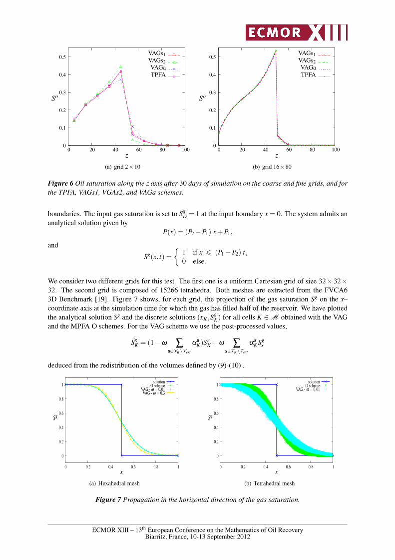
Figure 6 Oil saturation along the z axis after 30 days of simulation on the coarse and fine grids, and forthe TPFA, VAGs1, VGAs2, and VAGa schemes.

boundaries. The input gas saturation is set to SgD = 1 at the input boundary x = 0. The system admits an

analytical solution given byP(x) = (P2−P1) x+P1,

and

Sg(x, t) =

1 if x 6 (P1−P2) t,0 else.

We consider two different grids for this test. The first one is a uniform Cartesian grid of size 32×32×32. The second grid is composed of 15266 tetrahedra. Both meshes are extracted from the FVCA63D Benchmark [19]. Figure 7 shows, for each grid, the projection of the gas saturation Sg on the x–coordinate axis at the simulation time for which the gas has filled half of the reservoir. We have plottedthe analytical solution Sg and the discrete solutions (xK ,Sg

K) for all cells K ∈M obtained with the VAGand the MPFA O schemes. For the VAG scheme we use the post-processed values,

SgK = (1−ω ∑

s∈VK\Vext

αsK)Sg

K +ω ∑s∈VK\Vext

αsKSg

s

deduced from the redistribution of the volumes defined by (9)-(10) .

0

0.2

0.4

0.6

0.8

1

0 0.2 0.4 0.6 0.8 1

Sg

x

solutionO scheme

VAG - ω = 0.01VAG - ω = 0.3

(a) Hexahedral mesh

0

0.2

0.4

0.6

0.8

1

0 0.2 0.4 0.6 0.8 1

Sg

x

solutionO scheme

VAG - ω = 0.01

(b) Tetrahedral mesh

Figure 7 Propagation in the horizontal direction of the gas saturation.


The results presented in Figure 7 clearly show that, for each grid, the discrete solutions of both schemesintersect the analytical solution at the point (1

2 , 12), which exhibits that the velocity of the flow is well

approximated. On Figure 7(a), the solutions of the VAG scheme on the Cartesian grid is plotted for bothω = 0.01 and ω = 0.3 (9). The value ω = 0.3 roughly corresponds to match the pore volume of eachvertex φs with the pore volume of each surrounding cell φK , K ∈Ms. As expected, the choice ω = 0.3leads to a slightly less diffusive scheme than the VAG scheme with ω = 0.01. We note also that theVAG scheme is slightly less diffusive on such meshes than the MPFA O scheme (which degenerates forCartesian grids to the TPFA scheme). On the other hand, for the tetrahedral mesh, we can notice onFigure 7(b) that the VAG scheme is slightly more diffusive than the MPFA O scheme. This has beenobserved for both values of ω = 0.01 and 0.3. Note also that for both type of meshes the convergenceof the VAG scheme has been obtained numerically for both ω = 0.01 and ω = 0.3.

In terms of CPU time a ratio of 15 is observed between the simulation time obtained with the MPFA Oscheme on the tetrahedral mesh and the VAG scheme on the same mesh. This huge factor is due to thereduced size of the linear system obtained with the VAG scheme after elimination of the cell unknownscompared with the MPFA O scheme, both in terms of number of unknowns (around five time less forthe VAG scheme than for the MPFA O scheme) and in terms of number of non zero elements per line.

CO2 injection with dissolution and vaporization of H2O and salt precipitation

This test case simulates the nearwell injection of CO2 in a saline aquifer. Due to the vaporization ofH2O in the gas phase, the water phase is drying in the nearwell region leading to the precipitation ofthe salt dissolved in the water phase. This may result in a reduction of the nearwell permeability. Thisphenomenon could for example explain the loss of injectivity observed in the Tubaen saline aquifer ofthe Snohvit field in the Barents sea where around 700000 tons of CO2 are injected each year since 2008.

The model is a three phases (gas (g), water (w), mineral (m)) three components (CO2, H2O, salt) )compositional Darcy flow. It is assumed that the H2O component can vaporize in the gas phase and thatthe CO2 and salt components can dissolve in the water phase. It results that C w = H2O,CO2,salt,C g = H2O,CO2, and C m = salt where C α denotes the set of components may be present in thephase α . The mineral phase is immobile with a null relative permeability kr,m = 0, and the water and gas

phase relative permeabilities kr,α are non decreasing functions of the reduced saturation Sα =Sα

Sw +Sg ,α = w,g.

kr,α(Sα) =

(

Sα −Sr,α

1−Sr,α

)eα

if Sα ∈ [Sr,α ,1]

0 if Sα < Sr,α ,

with ew = 5, eg = 2, Sr,w = 0.3 and Sr,g = 0. The reference pressure is chosen to be the gas pressureP = Pg, and we set Pw = Pg +Pc,w(Sw) with

Pc,w(Sw) = Pc,1 log

(Sw−Sr,w

1−Sr,w

)−Pc,2,

for 1≥ Sw > Sr,w, where Pc,1 = 2.104 Pa, Pc,2 = 104 Pa. The thermodynamical equilibrium is modelledby equilibrium constants Hi of the component i such that

CgH2O = HH2O Cw

H2O in presence of both phases w and g,

CwCO2

= HCO2 CgCO2

in presence of both phases w and g,

Cwsalt = Hsalt in presence of both phases w and m.

where Cαi is the molar concentration of the component i in the phase α . The equilibrium constants will

be considered fixed in the range of pressure and temperature with the following values HH2O = 0.025,


HCO2 = 0.03 and Hsalt = 0.39 in kg/kg. Let us also denote the total molar fractions of the component i byZi and by Z = (Zi)i the vector of the total molar fractions. With these assumptions, the thermodynamicalflash, which gives the phases present, admits an analytical solution, independent of the pressure P, andwith entries Z in the two dimensional simplex

(ZCO2 ,Zsalt) |ZCO2 ≥ 0,Zsalt ≥ 0,1−ZCO2−Zsalt ≥ 0.

The solution is exhibited Figure 8 where we have set

E1 = (ECO2 HCO2 ,0), E2 = (ECO2 ,0), E3 = (DCO2 ,0), E4 = (0,Hsalt), E5 = (HCO2 DCO2 ,Hsalt),

with DCO2 =1−HH2O (1−Hsalt)

1−HH2O HCO2

and ECO2 =1−HH2O

1−HH2O HCO2

.

0

0.2

0.4

0.6

0.8

1

0 0.2 0.4 0.6 0.8 1E1

E3

E5E4

g+m

m

E2

g

w

w+m

w+g+m

w+g

ZCO2

Zsalt

Figure 8 Diagram of present phases in the space (ZCO2 ,Zsalt).

The 3D nearwell grids used for the simulation are exhibited in Figure 9. The first step of the discretiza-tion is to create a radial mesh, Figure 9(a), that is exponentially refined down to the well boundary. Thisnearwell radial local refinement is matched with the reservoir Ω = (−15,15)× (−15,15)× (−7.5,7.5)m3 using either hexahedra (see Figure 9(b)) or both tetrahedra and pyramids, (see Figure 9(c)). Theradius of the well is 10 cm and the radius of the radial zone is 5 m. The well is deviated by an angle of20 degrees away from the vertical axis z in the x,z plane. The hexahedral grid has 42633 cells and thehybrid grid 77599 cells.

(a) exponentially re-fined radial mesh

(b) unstructured mesh with onlyhexahedra

(c) hybrid mesh with hexahedra,tetrahedra and pyramids

Figure 9 Nearwell meshes.

The remaining of the data set and the boundary and initial conditions are the following. The porosity isset to Φ = 0.2, and the permeability tensor Λ is homogeneous and isotropic equal to 1. 10−12 m2. The


density and the viscosity of the water phase are computed by correlations function of P and Cw, andthose of the gas phase by linear interpolation in the pressure P, the density of the mineral phase is fixedto ρm = 2173 kg/l.

Homogeneous Neumann boundary conditions are imposed on the top and bottom boundaries. Along thewell boundary we impose the pressure P(x,y,z) = Pwell−ρg ‖ g ‖ z, with Pwell = 300 10+5 Pa, the inputphase Sg = 1 and its composition Cg

CO2= 1, Cg

H2O = 0. On the lateral outer boundaries (resp. at initialtime) the following hydrostatic pressure is imposed P(x,y,z) = P1−ρl ‖ g ‖ z, with P1 = Pwell− 10+5

Pa, as well as the following input (resp. initial) phase and its composition Sw = 1, CwH2O = 0.84 and

Cwsalt = 0.16.

The simulation time is fixed to 7 days in order to obtain a precipitation of the mineral up to around halfof the radial zone. To avoid too small control volumes in the nearwell region, the parameter ω has beenchosen in such a way that minK∈M ΦK = mins∈V Φs, leading in our case to ω ∼ 0.4.

We report in the table 1 below for both schemes and for both meshes the number of unknowns nu(#M for the MPFA O scheme and #Vint for the VAG scheme), the number nnz of nonzeros blocksin the Jacobian after elimination of the cell unknowns for the VAG scheme, the average number ofNewton iterations per time step nnl, and the average number of GMRES iterations per Newton stepnl. The stopping criteria in terms of relative residual for both the Newton convergence and the linearconvergence are set to 10−6. Note that the simulation with the MPFA O scheme on the hybrid meshcould not be obtained due to too high memory requirement for the matrix storage. The slight increase ofnonlinear iterations between the MPFA and the VAG scheme and between both meshes, as seen in table1, is probably due to the decrease of the control volume sizes.

Mesh-Scheme nu nnz nnl nlHexahedral-MPFA 42633 1100865 4.5 33Hexahedral-VAG 42756 1103310 4.8 35

Hybrid-MPFA 77599 4092027 - -Hybrid-VAG 37833 884577 5.4 38

Table 1 For both schemes and both meshes: number of unknowns nu, number nnz of nonzeros blocks inthe Jacobian, average number nnl of Newton iterations per time step, and average number nl of GMRESiterations per Newton step.

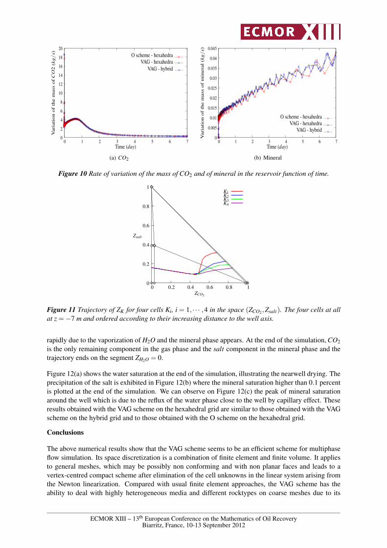
Figure 10 exhibits, for the two schemes and on both grids, the rate of variation of the masses of CO2and of the mineral in the reservoir function of time. We can notice that the VAG scheme solutions onboth meshes are almost the same and only slightly differ from the O scheme solution. The oscillationsobserved in Figure 10(b) are a well-known phenomenon due to the appearance of the mineral phase oneach successive cells when the salt reaches its maximum solubility.

Figure 11 exhibits the trajectory of the total mass fraction Z in the simplex (ZCO2 ,Zsalt) function of timefor four cells Ki, i = 1, · · · ,4. Starting from an initial state given by a single water phase and ZCO2 = 0,the mass of CO2 increases due to the injection. The CO2 is initially fully dissolved in the water phase,then the gas phase appears and its mass fraction θ g increases. As long as Cw

Salt is roughly constant, thetrajectory Z is close to the line defined by

ZCO2 = (1−θ g)CwCO2

+θ gCgCO2

,

Zsalt = (1−θ g)Cwsalt

since CwCO2

and CgCO2

are both fixed by Cwsalt and the thermodynamical equilibrium constants. Once

the water saturation Sw is close to the irreducible water saturation Sr,w, the composition Cwsalt increases


0

2

4

6

8

10

12

14

16

18

20

0 1 2 3 4 5 6 7

Time (day)

VAG - hexahedraO scheme - hexahedra

Var

iati

on

of

the

mas

so

fC

O2

(kg/

s)

VAG - hybrid

(a) CO2

0

0.005

0.01

0.015

0.02

0.025

0.03

0.035

0.04

0.045

0 1 2 3 4 5 6 7

Var

iati

on

of

the

mas

so

fm

iner

al(k

g/s)

Time (day)

VAG - hexahedraVAG - hybrid

O scheme - hexahedra

(b) Mineral

Figure 10 Rate of variation of the mass of CO2 and of mineral in the reservoir function of time.

0

0.2

0.4

0.6

0.8

1

0 0.2 0.4 0.6 0.8 1

ZCO2

K2K3K4

K1

Zsalt

Figure 11 Trajectory of ZK for four cells Ki, i = 1, · · · ,4 in the space (ZCO2 ,Zsalt). The four cells at allat z =−7 m and ordered according to their increasing distance to the well axis.

rapidly due to the vaporization of H2O and the mineral phase appears. At the end of the simulation, CO2is the only remaining component in the gas phase and the salt component in the mineral phase and thetrajectory ends on the segment ZH2O = 0.

Figure 12(a) shows the water saturation at the end of the simulation, illustrating the nearwell drying. Theprecipitation of the salt is exhibited in Figure 12(b) where the mineral saturation higher than 0.1 percentis plotted at the end of the simulation. We can observe on Figure 12(c) the peak of mineral saturationaround the well which is due to the reflux of the water phase close to the well by capillary effect. Theseresults obtained with the VAG scheme on the hexahedral grid are similar to those obtained with the VAGscheme on the hybrid grid and to those obtained with the O scheme on the hexahedral grid.

Conclusions

The above numerical results show that the VAG scheme seems to be an efficient scheme for multiphaseflow simulation. Its space discretization is a combination of finite element and finite volume. It appliesto general meshes, which may be possibly non conforming and with non planar faces and leads to avertex-centred compact scheme after elimination of the cell unknowns in the linear system arising fromthe Newton linearization. Compared with usual finite element approaches, the VAG scheme has theability to deal with highly heterogeneous media and different rocktypes on coarse meshes due to its


(a) reduced water saturation Sw (b) mineral saturation such that Sm >0.1%

(c) Cut of the mineral saturation Sm

Figure 12 Saturations at the end of the simulation.

flexibility in the definition of the porous volumes at the vertices.

The efficiency of our approach on complex meshes and for complex compositional models is exhibitedon three phases three components models which simulate the nearwell injection of miscible CO2 in asaline aquifer taking into account the vaporization of H2O in the gas phase as well a the deposition ofthe salt.

In order to better take into account discontinuous capillary pressures, a more advanced solution, follow-ing the recent work [8], would be to consider as vertex unknowns the capillary pressures rather than thesaturations, in such a way that the saturations at the vertices would be allowed to be discontinuous. Thisapproach will be developed in a future work.

Acknowledgments

The authors thank ANR VFSitCom, the COFFEE project of INRIA Sophia Antipolis, GNR MOMASand TOTAL for partially supported this work and TOTAL for permission to publish it.

References

[1] Aavatsmark, I., Barkve, T., Boe, O. and Mannseth, T. [1996] Discretization on non-orthogonal, quadrilateralgrids for inhomogeneous, anisotropic media. Journal of computational physics, 127(1), 2–14.

[2] Aavatsmark, I., Barkve, T., Boe, O. and Mannseth, T. [1998] Discretization on unstructured grids for inho-mogeneous, anisotropic media. part 1: Derivation of the methods. SIAM Journal on Scientific Computing,19, 1700.

[3] Aavatsmark, I., Eigestad, G., Mallison, B. and Nordbotten, J. [2008] A compact multipoint flux approx-imation method with improved robustness. Numerical Methods for Partial Differential Equations, 24(5),1329–1360.

[4] Agélas, L., Di Pietro, D. and Droniou, J. [2010] The g method for heterogeneous anisotropic diffusion ongeneral meshes. Mathematical Modelling and Numerical Analysis, 44(4), 597–625.

[5] Agélas, L., Di Pietro, D., Eymard, R. and Masson, R. [2010] An abstract analysis framework for noncon-forming approximations of diffusion on general meshes. International Journal on Finite Volumes, 7(1).

[6] Agélas, L., Guichard, C. and Masson, R. [2010] Convergence of finite volume mpfa o type schemes forheterogeneous anisotropic diffusion problems on general meshes. International Journal on Finite Volumes,7(2).

[7] Aziz, K. and Settari, A. [1979] Petroleum reservoir simulation. Applied Science Publishers.[8] Brenner, K., Cances, C. and Hilhorst, D. [2011] A convergent finite volume scheme for two-phase flows

in porous media with discontinuous capillary pressure field. Finite Volumes for Complex Applications VI-


Problems & Perspectives, 185–193.[9] Chen, Z. [2006] On the control volume finite element methods and their applications to multiphase flow.

Networks and Heterogeneous Media, 1(4), 689.[10] Edwards, M. and Rogers, C. [1994] A flux continuous scheme for the full tensor pressure equation. Proceed-

ings of ECMOR IV–4th European Conference on the Mathematics of Oil Recovery, EAGE, Roros, Norway.[11] Edwards, M. and Rogers, C. [1998] Finite volume discretization with imposed flux continuity for the general

tensor pressure equation. Computational Geosciences, 2(4), 259–290.[12] Eymard, R. and Gallouët, T. [1993] Convergence d’un schéma de type éléments finis-volumes finis pour

un système formé d’une équation elliptique et d’une équation hyperbolique. Modélisation mathématique etanalyse numérique, 27(7), 843–861.

[13] Eymard, R., Gallouët, T. and Herbin, R. [2000] Finite volume methods. Handbook of numerical analysis, 7,713–1018.

[14] Eymard, R., Gallouët, T. and Herbin, R. [2010] Discretization of heterogeneous and anisotropic diffusionproblems on general nonconforming meshes sushi: a scheme using stabilization and hybrid interfaces. IMAJournal of Numerical Analysis, 30(4), 1009–1043.

[15] Eymard, R., Guichard, C. and Herbin, R. [2011] Benchmark 3d: the vag scheme. Finite Volumes for ComplexApplications VI – Problems and Persepectives, Springer Proceedings in Mathematics, vol. 2, 213–222.

[16] Eymard, R., Guichard, C. and Herbin, R. [2012] Small-stencil 3d schemes for diffusive flows in porousmedia. ESAIM: Mathematical Modelling and Numerical Analysis, 46(02), 265–290.

[17] Eymard, R., Guichard, C., Herbin, R. and Masson, R. [2012] Vertex centred discretization of multiphasecompositional darcy flows on general meshes. Computational Geosciences, 1–19, ISSN 1420-0597.

[18] Eymard, R., Guichard, C., Herbin, R. and Masson, R. [2012] Vertex centred discretization of two-phasedarcy flows on general meshes. ESAIM: Proc., 35.

[19] Eymard, R., Henry, G., Herbin, R., Hubert, F., Klöfkorn, R. and Manzini, G. [2011] 3d benchmark ondiscretization schemes for anisotropic diffusion problems on general grids. Finite Volumes for Complex Ap-plications VI-Problems & Perspectives, 895–930.

[20] Huber, R. and Helmig, R. [2000] Node-centered finite volume discretizations for the numerical simulationof multiphase flow in heterogeneous porous media. Computational Geosciences, 141–164, ISSN 4.

[21] Peaceman, D. [1977] Fundamentals of numerical reservoir simulation, vol. 6. Elsevier.


vertex-centred discretization of multiphase compositional...

Documents