verteilte software-systeme im kontext von industrie 4.0

Verteilte Software-Systeme im Kontext von Industrie 4.0

Impulsvortrag

Dr. Peter Tröger

Technische Universität Chemnitz

7. Oktober 2014

Daimler, Oktober 2014

Industrie 4.0

• Forschungs- und Industrieagenda

• Zielsetzung

• Integration von (Echtzeit)-Daten aus verschiedenen Quellen

• Vernetzung von Mensch, Maschine, Objekten und IKT-Systemen

• Selbstoptimierende Prozesse

• Ermittlung und Ausnutzung von Verbesserungspotential

• Berücksichtigung der Mensch-Maschine-Schnittstelle

2[Bitcom, Fraunhofer IAO]


Industrie 4.0 - Für Informatiker

• Keine Monolithen mehr

• Flexibel koppelbare Software-Komponenten

• Funktionale Integration von Komponenten mit und ohne Echtzeitanforderungen

• Integration und Auswertung verschiedener Datenquellen

• Physische Sensoren und Aktuatoren

• Was bietet die Forschung ?

3[Bitcom, Fraunhofer IAO]

Daimler, Oktober 2014 4

Forschung

Verteilte Echtzeitsysteme

Skalierbareverteilte Systeme

Verfügbarkeit und Zuverlässigkeit


Skalierbare verteilte Systeme

• Coulouris et al.: „…[system] in which hardware or software components located at networked computers communicate and coordinate their actions only by passing messages…“

• Konsequenzen

• Nebenläufigkeit als Normalzustand, asynchrone Kommunikation

• Partielle Ausfälle

• Heterogenität, Sicherheit, Schutz, …

• Aktiver Gegenstand der Forschung

• Großer Hype um Big Data als ein Vertreter

5


Big Data• Was heißt „big“ ?

• Ein großes Berechnungsproblem ?

• „Viele“ Eingabedaten ?

• Strukturierte vs. unstrukturierte Daten

• Datenformate sind nichts Neues

• Problem des korrekten Einsatzes vonexistierenden Analyseansätzen

• Mathematiker und Statistiker sind gefragt

• Big data = Werkzeuge zur skalierbaren Datenverarbeitung

• Rechtfertigen die Datenmengen eigene Infrastrukturen ?

6


Big Data - Wie groß ist groß genug ?

[oracle.com]

„There are only two companies with a big data problem, Google and the NSA.“

http://oracle.com


Skalierbare verteilte Systeme

Load Balancing

Micro Services

Sharding

[microservices.io]


Architekturmuster: Micro Services

• „Feingranulare“ dienstorientierte Architektur (SOA)

• Kleine Dienste (services) und Komponenten

• Orientieren sich jeweils nur an einer geschäftlichen Funktion

• Einheitliches leichtgewichtiges Kommunikationsprotokoll (HTTP REST)

• Unabhängig und automatisch installierbar / aktualisierbar

• Programmiersprachen und Datenspeicherung sind lokale Entscheidung

• Führt typischerweise zur grobgranularer API (Overhead)

• Kein RPC über HTTP, sondern eher dokumentenorientiert

• „Smart endpoints, dumb pipe“ -> kein Enterprise Service Bus !

9



[Martin Fowler]



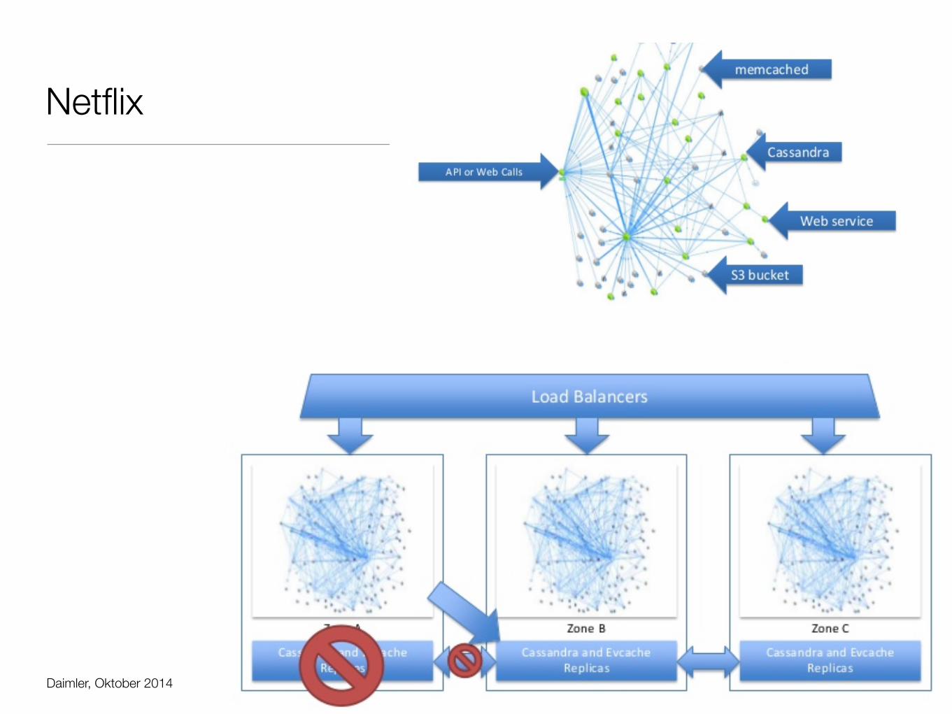
• Netflix

• 2008: Gesamte Funktionalität in einer Web Applikation

• 2012: Hunderte von Diensten auf AWS

• Entkoppeltes Ausrollen von Funktionen

• Dezentralisierte Verwaltung ist Pflicht (DevOps)

• Probleme mit Test und Schnittstellenversionierung

• Fehlertoleranz entsteht nicht automatisch

• Hystrix Projekt - Überwachung und Redundanz als Bibliothek für Entwickler

• Amazon: You built it, you run it.

• Entwickler sind für den Betrieb ihrer Teile zuständig -> DevOps in Industrie 4.0 ?

11


Netflix


Architekturmuster

• Content-based router

• Daten werden an funktionale Komponenten anhand ihrer Eigenschaften weitergeleitet

• Consumer-driven contracts

• Client-System liefertdem Dienst-Anbieter eineTest Suite mit den geforderten Erwartungen

• Ähnliche Idee: Tolerant reader

• Weak consistency

• Besseres Verständnis über geforderte Datenkonsistenz

• Eventual consistency: Keine Versprechen über Zeitverhalten („noSQL“)im verteilten System bei Aktualisierung der Daten

13


Forschung




• Neue Architekturmuster • Konsistenzmodelle • DevOps • Micro Services


Cyber-physische Systeme

• Vernetzung von physikalischen und technischen Elementen

• Vernetzung ohne zentrale Kontrolle (Autonomie)

• Sensoren und Aktuatoren auf physikalischer Ebene

• Kooperative Datenverarbeitung und Rückkoppelung an physikalische Welt

• Industrie 4.0 ?

• Verlässliche Maschine-zu-Maschine Kommunikation, leichte Rekonfiguration

• Vorhersagbare drahtlose Kommunikation im Produktionsumfeld

• Forschung

• Verteilte Mobilität ist noch nicht vollständig verstanden (Ortswechsel = Störung)

• Ziel: Awareness

15


[Acatech]



Internet der Dinge

• Verknüpfung von eindeutig identifizierbaren Gegenständen

• RFID, Strichcode, QR-Code

• Virtuelle Repräsentation in Internet-artiger Struktur

• Gemeinsame Konzepte

• Benennung (naming)

• Sensorik

• Informationsverarbeitung

• Kommunikation

• Neuer Anwendungsfall für bewährteKonzepte

17


IoT vs. CPS

‚Cyber‘ Entität



Physische Entität

Physische Entität

Physische Entität

Internet

Internetder Dinge



Beispiel: Time-Triggered Architecture [Kopetz]


Forschung




• Cyber-physischeSysteme

• Internet der Dinge • Temporale Firewalls • Mesh - Netzwerke



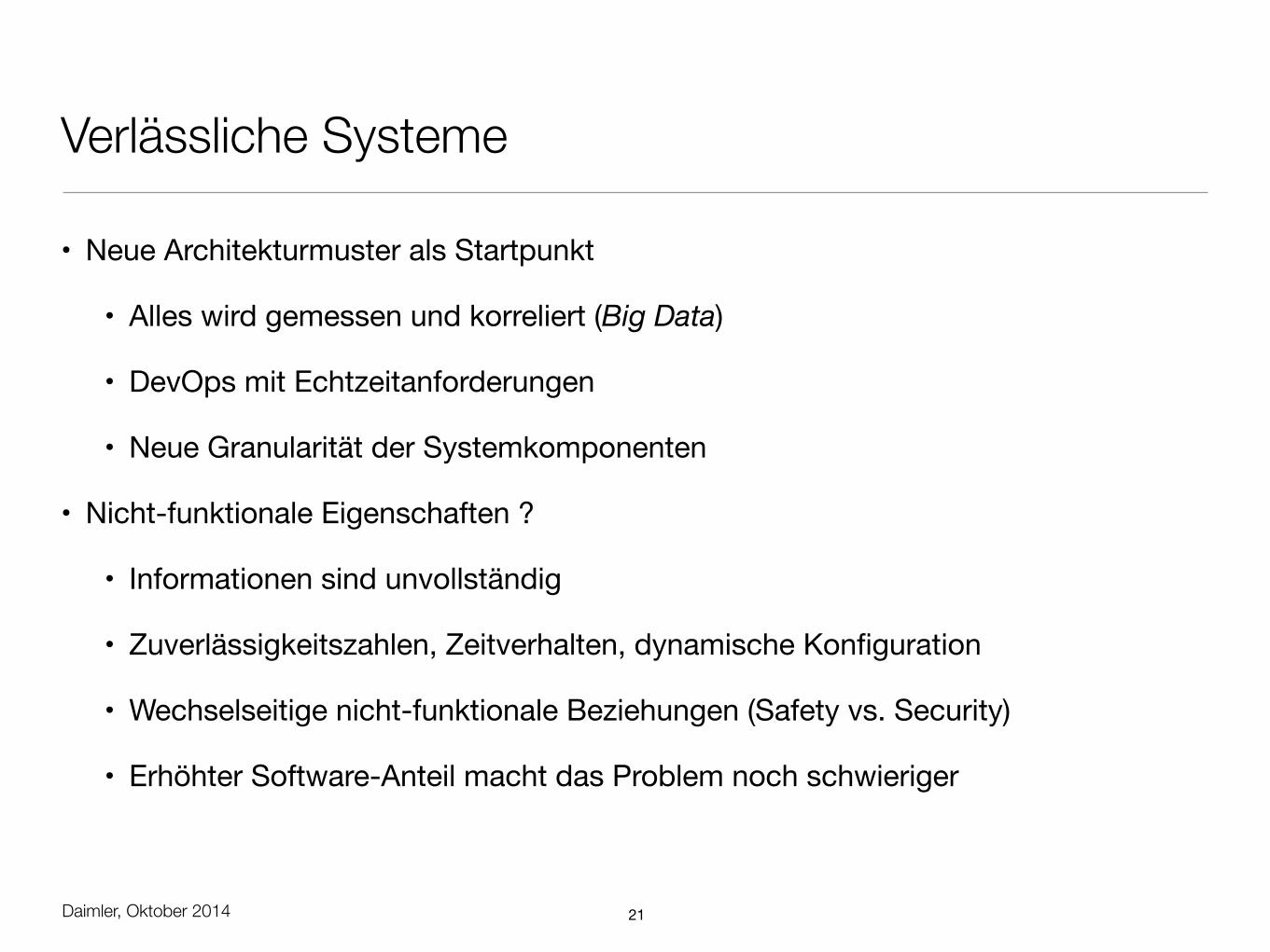
Verlässliche Systeme

• Neue Architekturmuster als Startpunkt

• Alles wird gemessen und korreliert (Big Data)

• DevOps mit Echtzeitanforderungen

• Neue Granularität der Systemkomponenten

• Nicht-funktionale Eigenschaften ?

• Informationen sind unvollständig

• Zuverlässigkeitszahlen, Zeitverhalten, dynamische Konfiguration

• Wechselseitige nicht-funktionale Beziehungen (Safety vs. Security)

• Erhöhter Software-Anteil macht das Problem noch schwieriger

21


Andere Domänen - Gleiches Problem


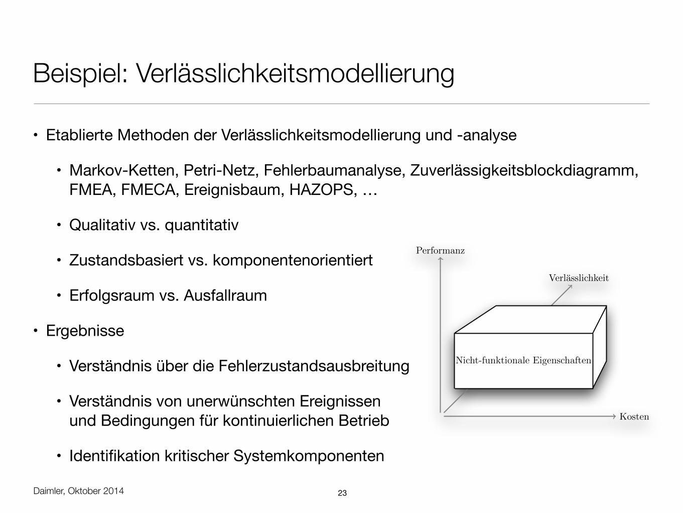
Beispiel: Verlässlichkeitsmodellierung

• Etablierte Methoden der Verlässlichkeitsmodellierung und -analyse

• Markov-Ketten, Petri-Netz, Fehlerbaumanalyse, Zuverlässigkeitsblockdiagramm, FMEA, FMECA, Ereignisbaum, HAZOPS, …

• Qualitativ vs. quantitativ

• Zustandsbasiert vs. komponentenorientiert

• Erfolgsraum vs. Ausfallraum

• Ergebnisse

• Verständnis über die Fehlerzustandsausbreitung

• Verständnis von unerwünschten Ereignissenund Bedingungen für kontinuierlichen Betrieb

• Identifikation kritischer Systemkomponenten

23

8 KAPITEL 1. TERMINOLOGIE

Kosten

Performanz

Verlasslichkeit

Nicht-funktionale Eigenschaften

Abbildung 1.1: Die Dimensionen der Verlasslichkeit, nach Malek.

Die beobachtete Funktionalitat wird an der Schnittstelle zum System bereitgestellt, womit der Nutzerkeine Informationen uber die internen Ablaufe hat (black box Prinzip). Die korrekte Funktionsweisemanifestiert sich daher nur im beobachtbaren Verhalten der Systemschnittstelle. Diese Entkopplung ander Systemschnittstelle ist die Grundlage fur verschiedenste Verlasslichkeitsmechanismen innerhalb einesSystems. Daher ist eine strikte Entkoppelung von Teilsystemen eine der wesentlichen Grundlagen furverlassliche Systeme.

Die Verlasslichkeit als nicht-funktionale Systemeigenschaft kann in Kombination mit anderen be-kannten Systemeigenschaften angestrebt werden. Prominentes Beispiel sind hier responsive Systeme [?],welche die Eigenschaften der Fehlertoleranz und des vorhersagbaren Zeitverhaltens kombinieren [TODO:bei Matthias nachschlagen].

Malek definiert die Verlasslichkeit als dritten Einflußfaktor der Systemqualitat neben den Kosten undder Leistungsfahigkeit des Systems (siehe Abbildung ??. Diese Beobachtung stellt einen wichtigen Aspektdar, da nahezu alle Methoden zur Verbesserung der Verlasslichkeit zusatzlichen Ressourcenbedarf und /oder gesteigerte Kosten implizieren. Die Abwagung von Kosten und Nutzen der Verlasslichkeit ist somitzentraler Bestandteil der notwendigen Architekturentscheidungen.

Aufgrund der hohen Relevanz von Verlasslichkeit fur viele Industriebereiche sind eine Vielzahl vonalternativen Definitionen durch Standardisierungsgremien entstanden. Tabelle ?? gibt einen Uberblickfur die Bandbreite der existierenden Definitionen. [TODO: Definitionen diskutieren]

ISO 9000:2005 [?] beschreibt Verlasslichkeit als zusammengesetztes Systemattribut, welches die Fahigkeitzur Sicherstellung von Wartbarkeit, Verfugbarkeit und Zuverlassigkeit beschreibt. Die letzteren Attributedefiniert der Standard als temporale Qualitatscharakteristiken, die neben den funktionalen, ergonomi-schen, physikalischen, sensorischen und den Verhaltenscharakteristiken existieren. Im Vergleich zur Defi-nition von Laprie et al. [?] wird Verlasslichkeit hier enger gefasst und bezieht sich auf die hauptsachlichinteressanten Aspekte in Hardware-Systemen.

Die MIL-STD-882D Spezifikation [?] des amerikanischen Verteidigungsministeriums beschreibt ei-ne standardisierte Vorgehensweise zur Sicherstellung von Systemsicherheit durch eine geeignete Risiko-abschatzung. Neben einem allgemeiner gefassten Systembegri↵, der auch Prozesse und Personen explizitmit einschliesst, wird der Begri↵ der Gefahrdung (hazard) als Beschreibung fur auslosende Faktoren einesSicherheitsproblems definiert. Der Sicherheitsausfall selbst wird dann als Mishap bezeichnet.

Abbildung ?? fasst die verschiedenen Aspekte der Verlasslichkeit zusammen, die in den folgendenAbschnitten erlautert werden.

1.1 Bedrohungen der Verlasslichkeit

Die Bedrohungen der Verlasslichkeit sind unerwunschte Beeinflussungen oder Anderungen im System,welche die spezifikationskonforme Diensterbringung jetzt oder in Zukunft beeintrachtigen. Laprie et al.


Problem #1 - Konfigurierbarkeit

• Eigenschaften moderner technischer Systeme

• Stetig zunehmende Komplexität von Software und Hardware

• Zunehmender Anteil von Software

• Modularisierte Architekturen mit optionalen Komponenten

• Beispiele: Fahrzeugelektronik, Telefone, eingebettete Steuerungsanlagen, medizinische Geräte, Industrieautomatisierung, …

• Flexible Konfiguration

• Grad der Redundanz ist frei wählbar

• Aufrüstung mit neueren / unbekannten Komponenten

• Variabler Funktionsumfang

24


Problem #2 - Fehlende Daten

• Quantitative Verlässlichkeitsanalyse für komplexe Systeme

• Schnellere Produktzyklen mit signifikanten Zeitdruck

• Unpräzise Architekturmerkmale

• Finale Auswahl der verwendeten Komponenten relativ spät

• RAS-Analyse ist selten Teil des Budget, eher ‚Nebentätigkeit‘

• Vertrauenswürdige Zuverlässigkeitsdaten als Unsicherheitsfaktor

• Einige Domänen müssen das Investment leisten (Sicherheit, sensible Anwendungen)

• Viele sind dazu nicht in der Lage

• Typischerweise Beschränkung auf rein qualitative Analyse

25


Beispiel: Verlässlichkeitsmodellierung

• Vorschlag: Unterstützung für unpräzise Modellierung

• Expliziter Umgang mit partiellen Systemwissen

• Unsicherheit als expliziten Teil der Analyse betrachten

• Unterstützung von inkrementeller Verbesserung und iterativer Wissenserweiterung

• Fokus auf relative Vergleiche, kein „numbers game“

• Ingenieure bevorzugen nicht-zustandsbasierte Modelle

• FuzzTrees - Erweitere Fehlerbaumnotation

• Analyse von konfigurierbaren Systemen

• Nutzung von Methoden der Fuzzy Logik

26

http

://am

ybru

cker

.com

/

P. Tröger, F. Becker, and F. Salfner, “FuzzTrees - Failure Analysis with Uncertainties,” in 19th Pacific Rim International Symposium on Dependable Computing (PRDC), 2013.

http://amybrucker.com


FuzzTree Notation

27

as basic event probability (e.g. in fault trees), a reasonablequantitative analysis can only be realized if all the precisenumbers are available. This renders such modeling infeasiblein many cases, or makes it at least a very costly activity.Moreover, in early phases of a system design, such numbersmight not be obtainable at all, since some componentsmight not even have been built, yet. Feedback from industryshows that this prerequisite often leads to the sole usageof qualitative methods such as FMEA. Many safety-relatedindustries still have to pay the price for getting trustworthyreliability data, but the pace of hardware and softwareevolution makes it difficult, even for them, to maintain thenecessary analysis quality.

Due to our understanding of the situation in engineeringpractice, we argue that quantitative modeling should evolveto become applicable even under conditions of imprecisesystem knowledge. We propose to make uncertainty explicitas part of the dependability analysis, in order to supportincremental knowledge improvements not only of the systemdesign, but also of the dependability model.

In this article, we describe a first step into this directionby extending fault tree modeling in a way to embrace un-certainty. Our contribution is an extended fault tree notationfor expressing configurable systems, combined with a quan-titative analysis method that considers imprecise probabilitydata. This paper corrects and supersedes the initial FuzzTreesidea sketched in [3].

II. THE FUZZTREE NOTATION

A fault tree is a graphical model that shows the causal de-pendencies of faults potentially contributing to an undesiredfailure event. A fault tree analysis is carried out in multiplesteps, which include the definition of boundary conditions,the tree construction based on a given system design, thedetermination of cut sets, and the qualitative and quantitativeanalysis [4]. A static fault tree1 can contain primary events,such as basic events or undeveloped events, intermediateevents, gates connecting lower-level events to higher-levelevents, and transfer symbols [5]. Fault events are treated asbinary, meaning that they may or may not occur.

Our FuzzTree concept is an extension of the classical faulttree notation. The main idea is to support high-level modelsthat can be instantiated with multiple system configurations.A system configuration is the set of choices made foreach configurable component or subsystem. By picking onespecific system configuration, a FuzzTree instance is created.The supported set of configurations for a component orsubsystem is assumed to be known at modeling time, whileit is unknown which specific configuration will finally beused in operation. Instead of creating a fault tree for eachpossible system configuration, our notation is now intended

1We treat dynamic fault trees as being out of scope for this article.

N: 4-5k: N-2

Secondary CPUFailure

p=0.08 ± 0.008

Primary CPUFailure

p=0.08 ± 0.008

Server Failure

Power UnitFailure

p=0.15 ± 0.05

RAID 0 Failure RAID 1 Failure

Disc Failurep=0.12 ± 0.01

#2


#2

Figure 1. A FuzzTree example. Dashed lines visualize the variation points.

to allow a condensed notation and evaluation of all thepossible variations.

We explain the extended notation based on a minimalexample shown in Figure 1. The tree describes a small partof a real-world server system that has three different systemdesign variation points:

• The system could be equipped with a second CPU thatacts as a redundant unit for the primary CPU.

• The number of power units used in the system isflexible. At least three of the N power units mustalways work to have a running system, so N �3 is themaximum number of units that is allowed to fail for astill-working system. Moving that to failure space, weneed at least k = N �3+1 failing power units to havea failing power supply.

• The system has two discs, which can be either operatedin RAID 0 (striping) mode or RAID 1 (mirroring)mode.

It must be noted that the over-simplified example waschosen for clarity and space reasons. The general approachhas also shown to be valid for more realistic and largermodels in practice.

Our FuzzTree example can be unfolded into a set ofclassical fault trees described in Table I. Each of these

11.02.13 FuzzEd - Server Failure (1xCPU, N=4, RAID 0)

fuzztrees.net/editor/43 1/1

Primary CPUFailure

Server Failure

Disc Failure#2

RAID 0

Power UnitFailure

#4

k/N: 2-4



Disc Failure#2

RAID 1

Power UnitFailure

#4

k/N: 2-4Primary CPUFailure

Server Failure



Primary CPUFailure

Server Failure

Disc Failure#2

RAID 0

Power UnitFailure

#5

k/N: 3-5



Primary CPUFailure

Server Failure

Disc Failure#2

RAID 1

Power UnitFailure

#5

k/N: 3-5




Primary CPUFailure

Server Failure

Disc Failure#2

RAID 0

Power UnitFailure

#4

k/N: 2-4




Primary CPUFailure

Server Failure

Disc Failure#2

RAID 1

Power UnitFailure

#4

k/N: 2-4



k/N: 3-5


Primary CPUFailure

Server Failure

Disc Failure#2

RAID 0

Power UnitFailure

#5

Server Failure

k=3

Primary CPUFailure


Power UnitFailure

#5

RAID 1

Disc Failure#2

Fehler-bäume

Inclusion Variation Point

Redundancy Variation Point

Feature Variation Point


Quantitative Analyse

as basic event probability (e.g. in fault trees), a reasonablequantitative analysis can only be realized if all the precisenumbers are available. This renders such modeling infeasiblein many cases, or makes it at least a very costly activity.Moreover, in early phases of a system design, such numbersmight not be obtainable at all, since some componentsmight not even have been built, yet. Feedback from industryshows that this prerequisite often leads to the sole usageof qualitative methods such as FMEA. Many safety-relatedindustries still have to pay the price for getting trustworthyreliability data, but the pace of hardware and softwareevolution makes it difficult, even for them, to maintain thenecessary analysis quality.

Due to our understanding of the situation in engineeringpractice, we argue that quantitative modeling should evolveto become applicable even under conditions of imprecisesystem knowledge. We propose to make uncertainty explicitas part of the dependability analysis, in order to supportincremental knowledge improvements not only of the systemdesign, but also of the dependability model.

In this article, we describe a first step into this directionby extending fault tree modeling in a way to embrace un-certainty. Our contribution is an extended fault tree notationfor expressing configurable systems, combined with a quan-titative analysis method that considers imprecise probabilitydata. This paper corrects and supersedes the initial FuzzTreesidea sketched in [3].

II. THE FUZZTREE NOTATION

A fault tree is a graphical model that shows the causal de-pendencies of faults potentially contributing to an undesiredfailure event. A fault tree analysis is carried out in multiplesteps, which include the definition of boundary conditions,the tree construction based on a given system design, thedetermination of cut sets, and the qualitative and quantitativeanalysis [4]. A static fault tree1 can contain primary events,such as basic events or undeveloped events, intermediateevents, gates connecting lower-level events to higher-levelevents, and transfer symbols [5]. Fault events are treated asbinary, meaning that they may or may not occur.

Our FuzzTree concept is an extension of the classical faulttree notation. The main idea is to support high-level modelsthat can be instantiated with multiple system configurations.A system configuration is the set of choices made foreach configurable component or subsystem. By picking onespecific system configuration, a FuzzTree instance is created.The supported set of configurations for a component orsubsystem is assumed to be known at modeling time, whileit is unknown which specific configuration will finally beused in operation. Instead of creating a fault tree for eachpossible system configuration, our notation is now intended

1We treat dynamic fault trees as being out of scope for this article.

N: 4-5k: N-2


p=0.08 ± 0.008

Primary CPUFailure

p=0.08 ± 0.008

Server Failure

Power UnitFailure

p=0.15 ± 0.05

RAID 0 Failure RAID 1 Failure


#2


#2

Figure 1. A FuzzTree example. Dashed lines visualize the variation points.

to allow a condensed notation and evaluation of all thepossible variations.

We explain the extended notation based on a minimalexample shown in Figure 1. The tree describes a small partof a real-world server system that has three different systemdesign variation points:

• The system could be equipped with a second CPU thatacts as a redundant unit for the primary CPU.

• The number of power units used in the system isflexible. At least three of the N power units mustalways work to have a running system, so N �3 is themaximum number of units that is allowed to fail for astill-working system. Moving that to failure space, weneed at least k = N �3+1 failing power units to havea failing power supply.

• The system has two discs, which can be either operatedin RAID 0 (striping) mode or RAID 1 (mirroring)mode.

It must be noted that the over-simplified example waschosen for clarity and space reasons. The general approachhas also shown to be valid for more realistic and largermodels in practice.

Our FuzzTree example can be unfolded into a set ofclassical fault trees described in Table I. Each of these

0

1

0.05 0.1 0.15 0.2 0.25x

µ

CPU FailureDisc Failure

Power Unit Failure

Figure 8. Membership functions for the example

existing efficient solutions, such as the one by Rushdi etal. [13].

For the XOR gate case, the restriction of the possible com-binations is not possible, so all of them must be considered.Beside that, the approach is equivalent to the k-out-of-Ncase.

A. Example

Continuing with our illustrating example in Figure 1, weassume some fuzzy membership functions for the probabil-ities of CPU, disc and power failures (see also Figure 8):

• P (“CPU Failure”) = tfn(0.072, 0.08, 0.088)• P (“Power Unit Failure”) = tfn(0.1, 0.15, 0.2)• P (“Disc Failure”) = tfn(0.11, 0.12, 0.13)

We pick a rather low decomposition number of m = 2,here resulting in three ↵-cuts that need to be computed.Table II lists the resulting intervals for each ↵-cut. As thecalculation follows the same principle for each value of ↵,we only show computations for ↵ = 0. The same holds forthe various system configurations, where we only focus onthe (2-4-0) configuration.

Table IIINTERVALS FOR THE ↵-CUTS OF THE BASIC EVENTS IN (2-4-0).

↵ CPU Failure Power Unit Failure Disc Failure

0.0 [0.072, 0.088] [0.100, 0.200] [0.110, 0.130]0.5 [0.076, 0.084] [0.125, 0.175] [0.115, 0.125]1.0 [0.080, 0.080] [0.150, 0.150] [0.120, 0.120]

In the given example, the top event may happen if eitherboth CPUs, at least 2 out of 4 power units, or one of thediscs fail:

X = C _ P _ S

C represents the AND-combination of the two CPUfailures, P is the k-out-of-N gate for the power subsystemfailure and S is the result of the RAID 0 failure event.

The AND gate value for C is determined by multiplyingthe intervals with each other. For the OR-gate of S, theintersection of the boundary values has to be subtracted as

described above:C = [0.072, 0.088] · [0.072, 0.088]

= [0.005184, 0.007744]

S = [0.11, 0.13] _ [0.11, 0.13]

= [0.11 + 0.11� 0.11 · 0.11, 0.13 + 0.13� 0.13 · 0.13]= [0.2079, 0.2431]

The “2-out-of-4” gate for P can be computed as union of“exactly 2-out-of-4”, “exactly 3-out-of-4” and “4-out-of-4”:

P = 6 · [0.1, 0.2]2 · (1� [0.1, 0.2])

2+

4 · [0.1, 0.2]3 · (1� [0.1, 0.2]) + 1 · [0.1, 0.2]4

= [0.0523, 0.1808]

The interval describing the 0-cut for the top event fuzzyprobability then equals:

X = C _ P _ S = (C _ P ) _ S

= [0.057212877, 0.187143885] _ S

= [0.25321832, 0.384749206]

The same computation has to be performed for ↵ = 0.5

and ↵ = 1.0 per instance, resulting in the complete resultas shown in Table III and Figure 9.

Table III↵-CUTS FOR ALL SYSTEM CONFIGURATIONS.

FuzzTree ↵ = 0.0 ↵ = 0.5 ↵ = 1.0

(2-4-0) [.25322, .38475] [.28271, .34901] [.31482, .31482](1-4-0) [.30338, .43451] [.33337, .39946] [.36558, .36558](2-5-0) [.21875, .29246] [.2338, .27057] [.25103, .25103](1-5-0) [.27122, .34969] [.28792, .3271] [.30651, .30651](2-4-1) [.06862, .20088] [.09629, .16302] [.12796, .12796](1-4-1) [.13118, .26552] [.16012, .22787] [.19255, .19255](2-5-1) [.02563, .08101] [.03467, .06217] [.04677, .04677](1-5-1) [.09108, .15534] [.10286, .13484] [.11738, .11738]

It can be seen that the most reliable configuration is(2-5-1), which is not surprising and could have been alsodetermined by manual inspection. However, other questionsare harder to answer without analytical support, such as if “itis more reliable to use two CPUs with RAID 0, or one CPUwith RAID 1?”. The example also shows how FuzzTrees canbe a solution for reliability modeling with highly complexand configurable systems.

B. Cost-Based AnalysisFuzzTrees can be easily extended with a notion of costs,

were each basic event gets an according indication. Thiswould express the necessary investment to include the eventsource component, with a certain unreliability, into one sys-tem configuration. The total cost of one system configurationcan then be computed by combining all costs of basic

0

1

0.05 0.1 0.15 0.2 0.25x

µ

CPU FailureDisc Failure

Power Unit Failure

Figure 8. Membership functions for the example

existing efficient solutions, such as the one by Rushdi etal. [13].

For the XOR gate case, the restriction of the possible com-binations is not possible, so all of them must be considered.Beside that, the approach is equivalent to the k-out-of-Ncase.

A. Example

Continuing with our illustrating example in Figure 1, weassume some fuzzy membership functions for the probabil-ities of CPU, disc and power failures (see also Figure 8):

• P (“CPU Failure”) = tfn(0.072, 0.08, 0.088)• P (“Power Unit Failure”) = tfn(0.1, 0.15, 0.2)• P (“Disc Failure”) = tfn(0.11, 0.12, 0.13)

We pick a rather low decomposition number of m = 2,here resulting in three ↵-cuts that need to be computed.Table II lists the resulting intervals for each ↵-cut. As thecalculation follows the same principle for each value of ↵,we only show computations for ↵ = 0. The same holds forthe various system configurations, where we only focus onthe (2-4-0) configuration.

Table IIINTERVALS FOR THE ↵-CUTS OF THE BASIC EVENTS IN (2-4-0).

↵ CPU Failure Power Unit Failure Disc Failure

0.0 [0.072, 0.088] [0.100, 0.200] [0.110, 0.130]0.5 [0.076, 0.084] [0.125, 0.175] [0.115, 0.125]1.0 [0.080, 0.080] [0.150, 0.150] [0.120, 0.120]

In the given example, the top event may happen if eitherboth CPUs, at least 2 out of 4 power units, or one of thediscs fail:

X = C _ P _ S

C represents the AND-combination of the two CPUfailures, P is the k-out-of-N gate for the power subsystemfailure and S is the result of the RAID 0 failure event.

The AND gate value for C is determined by multiplyingthe intervals with each other. For the OR-gate of S, theintersection of the boundary values has to be subtracted as

described above:C = [0.072, 0.088] · [0.072, 0.088]

= [0.005184, 0.007744]

S = [0.11, 0.13] _ [0.11, 0.13]

= [0.11 + 0.11� 0.11 · 0.11, 0.13 + 0.13� 0.13 · 0.13]= [0.2079, 0.2431]

The “2-out-of-4” gate for P can be computed as union of“exactly 2-out-of-4”, “exactly 3-out-of-4” and “4-out-of-4”:

P = 6 · [0.1, 0.2]2 · (1� [0.1, 0.2])

2+

4 · [0.1, 0.2]3 · (1� [0.1, 0.2]) + 1 · [0.1, 0.2]4

= [0.0523, 0.1808]

The interval describing the 0-cut for the top event fuzzyprobability then equals:

X = C _ P _ S = (C _ P ) _ S

= [0.057212877, 0.187143885] _ S

= [0.25321832, 0.384749206]

The same computation has to be performed for ↵ = 0.5

and ↵ = 1.0 per instance, resulting in the complete resultas shown in Table III and Figure 9.

Table III↵-CUTS FOR ALL SYSTEM CONFIGURATIONS.

FuzzTree ↵ = 0.0 ↵ = 0.5 ↵ = 1.0

(2-4-0) [.25322, .38475] [.28271, .34901] [.31482, .31482](1-4-0) [.30338, .43451] [.33337, .39946] [.36558, .36558](2-5-0) [.21875, .29246] [.2338, .27057] [.25103, .25103](1-5-0) [.27122, .34969] [.28792, .3271] [.30651, .30651](2-4-1) [.06862, .20088] [.09629, .16302] [.12796, .12796](1-4-1) [.13118, .26552] [.16012, .22787] [.19255, .19255](2-5-1) [.02563, .08101] [.03467, .06217] [.04677, .04677](1-5-1) [.09108, .15534] [.10286, .13484] [.11738, .11738]

It can be seen that the most reliable configuration is(2-5-1), which is not surprising and could have been alsodetermined by manual inspection. However, other questionsare harder to answer without analytical support, such as if “itis more reliable to use two CPUs with RAID 0, or one CPUwith RAID 1?”. The example also shows how FuzzTrees canbe a solution for reliability modeling with highly complexand configurable systems.

B. Cost-Based AnalysisFuzzTrees can be easily extended with a notion of costs,

were each basic event gets an according indication. Thiswould express the necessary investment to include the eventsource component, with a certain unreliability, into one sys-tem configuration. The total cost of one system configurationcan then be computed by combining all costs of basic

0.02 0.04 0.06 0.08 0.1 0.12 0.14 0.16 0.18 0.2 0.22 0.24 0.26 0.28 0.3 0.32 0.34 0.36 0.38 0.4 0.42 0.44

0

1

(2-4-0) (1-4-0)(2-5-0) (1-5-0)(2-4-1) (1-4-1)(2-5-1) (1-5-1)

x

µ

Figure 9. The resulting top event fuzzy probabilities for all system configurations (a)–(h).

events and the costs associated with this configuration onthe transfer-in gates.

For inclusion variation points, the costs of an event areadded to the system costs if the configuration includes thisevent. For feature variation points, the costs of the chosenchild tree contribute to the system costs.

In the case of a redundancy variation, the chosen k valueleads to an according cost contribution in the particularconfiguration. In the most simple case, the resulting costequals k times the cost of a single unit. However, moredifficult cases may exist in which there is a non-linearrelationship to k. This could be expressed by a cost formulaper variation point.

Including costs directly in the analysis would allow tobuild tools that determine information such as the cheapestlevel of redundancy, the cost / reliability impact of optionalfeatures, or the cost / reliability impact of feature choices.A system designer would be also able to set the targetreliability of the system, for example according to someservice-level agreement, and let the FuzzTree tool chainsearch for the cheapest system configuration to achieve thereliability target. One interesting aspect of such a tradeoffanalysis is that higher costs do not always result in betterreliability. These cases typically appear if variation pointsexist that target at improving the system’s performance orfunctionality.

V. RELATED WORK

Fault tree modeling is a well-researched technique thatwas invented by H. A. Watson in the Bell Labs in 1961 [14].The approach is a standard in all safety-related industries,were risk assessment and error propagation analysis ismandated by standards and laws [15].

The idea for inclusion and feature variation points inFuzzTrees was driven by research in the field of variabilitymodeling for complex software systems [16]. Many model-ing approaches in this area focus on the extension of UMLtowards feature diagrams [17].

It can be argued that variation points may not be neededwhen the automated generation of fault trees from systemdescriptions or software artifacts would work sufficientenough. Since several decades of research did not leadto broadly adopted and accepted solution for this problem[15], we still see a need for optimized “manual” modeling

concepts. The automated generation of FuzzTrees, insteadof fault trees, would also allow a more concise graphicalnotation of todays complex systems.

Kaiser et al. introduced a component concept for faulttrees [18], which allows to partition fault trees into in-dependent components connected by ports. This techniqueallows a more realistic representation of system structures,but still does not consider the configurability of each systemcomponent.

Walter et al. [19] developed the LARES description lan-guage, which allows the specification of systems with con-ditional behavior in error situations. However, the dynamicbehavioral description is currently fixed for one layout of thesystem. We assume that the extension of LARES towardsreconfigurable systems would be extremely easy, whichmakes the formalism an interesting “textual counterpart” forFuzzTrees. LARES does not support fuzzy probabilities.

The concept of extended fault trees (eFT), as introducedby Buchacker et al. [20], allows to extend the description ofevent nodes using finite automata. This enables the reliabilityengineer to formulate dependencies and interactions of spe-cific failure modes in the tree leaves. The eFT is helpfulto make complex error propagation effects or commoncause issues more explicit, which is a different target incomparison to our uncertainty consideration goal.

Bobbio et al. discussed in several articles the conceptof parametric fault trees [21]. Such trees allow avoidingredundant sub-tree layouts by folding them into a more com-pact representation. This is achieved by adding a replicatorevent that indicates the root of a replicated sub-tree withsome parametrization. Like FuzzTrees, the approach targetsthe complexity issue of fault trees for modern systems,but mainly reformulates the same failure equation whereasFuzzTrees can handle structurally different sub trees.

The notion of uncertainty is not new in dependabilitymodeling research. A typical example is the concept ofuncertainty importance measures [22], [23], [24]. Thesemetrics rely on the formulation of model input, in ourcase the basic event rate or probability, as a random valuethat follows a certain probability distribution function. Thisallows, beside other things, the derivation of uncertaintycontributions for basic events with respect to the top event.We argue here that the inclusion of even more unknownprobability distributions as part of the model does not help


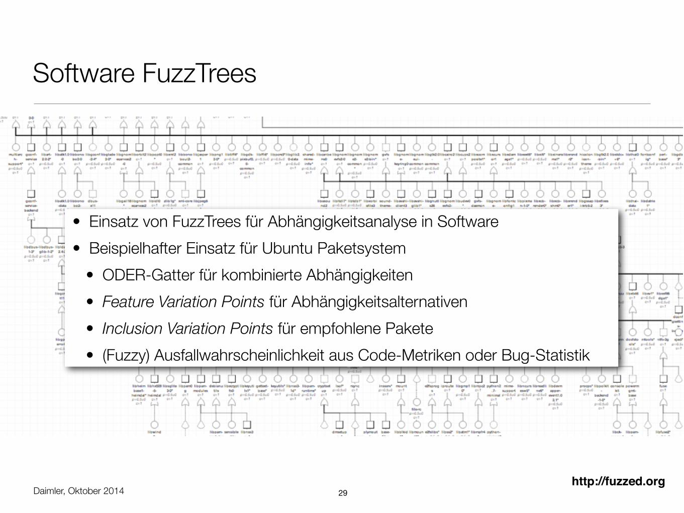
Software FuzzTrees

29

• Einsatz von FuzzTrees für Abhängigkeitsanalyse in Software • Beispielhafter Einsatz für Ubuntu Paketsystem

• ODER-Gatter für kombinierte Abhängigkeiten • Feature Variation Points für Abhängigkeitsalternativen • Inclusion Variation Points für empfohlene Pakete • (Fuzzy) Ausfallwahrscheinlichkeit aus Code-Metriken oder Bug-Statistik

http://fuzzed.org


Beispiel: Proaktive Fehlertoleranz

• Reaktive Fehlertoleranz hat Skalierbarkeitsprobleme

• Dauer der Fehlererholung korreliert mit Systemgröße, CAP-Theorem

• 24/7 Verfügbarkeit im Geschäftsumfeld

• Proaktive Fehlertoleranz reagiert ‚im Voraus‘

30

Fehlertoleranz

Latente Fehlerursache

Fehler-zustand

Normal-betrieb

Aktivierung

Erkennung

Ausfall



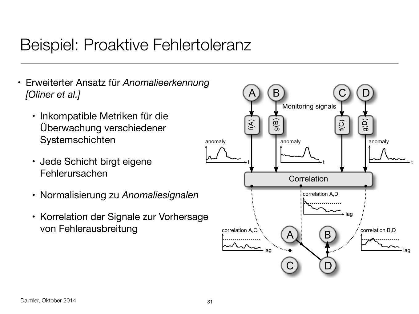
• Erweiterter Ansatz für Anomalieerkennung[Oliner et al.]

• Inkompatible Metriken für die Überwachung verschiedenerSystemschichten

• Jede Schicht birgt eigene Fehlerursachen

• Normalisierung zu Anomaliesignalen

• Korrelation der Signale zur Vorhersagevon Fehlerausbreitung

31

� � � �

��

� �

� �

��

��

��

��

��

��

��

��

��

��

��

��

��



!"#$

%&'()*(+&,$-**$

!.'($!.'($

!.'($!.'($

*&/01

.&'2$

3(4/5(6$

78$

9::

,/5&;

.0$8('4('$

78$

<.'=,.&2$

9::

,/5&;

.0$8('4('$

<.'=,.&2$

-/'+>&,/?&;.0$!,>6+('$*&0&@(A(0+$

Phy

sica

l Mac

hine

Sta

tus

Virtu

al M

achi

ne S

tatu

s

B(&,+C$D02/5&+.'$E&'@(+$*&5C/0($85C(2>,('$*/@'&;.0$!.0+'.,,('$

"'()2/5+.'6$

"'()2/5+.'6$

B&'2F&'($,(4(,G$!"#$%"&'%&()*+,-.$%/&!/%

B&'2F&'($,(4(,G$!"#$%"&'%&()*+,-.$%/&!/%

B&'2F&'(G$!"#$%"&'%&()*+,-.$%/&!/%

"'()2/5+.'6$

"'()2/5+.'6$

"'()2/5+.'6$

B&'2F&'($,(4(,G$!"#$%"&'%&()*+,-.$%/&!/%

B&'2F&'($,(4(,G$!"#$%"&'%&()*+,-.$%/&!/%-/'+>&,$*&5C/0($*.0/+.'G$-:'.1(H$0123)4$%4()5%

"'()2/5+.'6$

"'()2/5+.'6$

"'()2/5+.'6$

B&'2F&'($,(4(,G$!"#$%"&'%&()*+,-.$%/&!/%

B&'2F&'($,(4(,G$!"#$%"&'%&()*+,-.$%/&!/%

7:('&;0@$8I6+(AG$63(750$%8,-6)91%!)-,3)(,-.%:0(-0+%

"'()2/5+.'6$

"'()2/5+.'6$

"'()2/5+.'6$

B&'2F&'($,(4(,G$!"#$%"&'%&()*+,-.$%/&!/%

B&'2F&'($,(4(,G$!"#$%"&'%&()*+,-.$%/&!/%

9::,/5&;.0$J$*/22,(F&'(G$#44+,57;)-$%#44<0(=0($%><?@AA%

"'()2/5+.'6$

"'()2/5+.'6$

F. Salfner and P. Tröger, “Predicting Cloud Failures Based on Anomaly Signal Spreading,” in 42nd Annual IEEE/IFIP International Conference on Dependable Systems and Networks (DSN), 2012.


Beispiel: DFD-basierte Schutzanalyse

K. Schmidt, P. Tröger, H.-M. Kroll, T. Bünger, F. Krüger, and C. Neuhaus, “Adapted Development Process for Security in Networked Automotive Systems,” in SAE World Congress, 2014.


„Auf den Schultern von Giganten“



Verlässliche(dynamische) Systeme

• Unscharfe Verlässlichkeitsmodellierung

• Ausfallvorhersage • Anomalieerkennung

• Cyber-physischeSysteme

• Internet der Dinge • Temporale Firewalls • Mesh - Netzwerke



Kontaktdaten

Dr. Peter Tröger

Akademischer Assistent(assistant professor)

Technische Universität ChemnitzFakultät für InformatikProfessur BetriebssystemeStraße der Nationen 62, Haus C09111 Chemnitz

Tel.: +49 371 531 36181Fax: +49 371 531 836181

[email protected]@ptroeger

35