MODRETVERSION 6.0

FOR WINDOWS 95

EXPLANATIONS FOR MENU COMMAND OPTIONS

FIRST SCREEN PROMPT

Setup Hydrograph Infiltration Routing Graphic Windows ReadMe

Select one of these options using the mouse and click the left button or press the underlined letter.Similarly, all subsequent menu selections can be activated the same way. For a brief descriptionof model capability, refer to What's New in Version 6.0 in the preceding section of this manual.

1.0 Setup

Font Setup...Print Setup...

Working Directory...

Exit

Under this option, the model allows setup of fonts, printer and working directory, as wells as anoption to exit the MODRET program. In general, these options allow organization of the workingenvironment for a particular project and setting up the printing conditions. Simply click on theSetup button, select the desired option and click again using standard Windows 95 environment.Then select the desired font, printer and directory options.

2.0 Hydrograph

New **

Open **

Delete

2.1 New

Selecting the Hydrograph option, the next level of options are displayed. To go to previouscommand line, press Esc or select options using the mouse. Clicking on the New button, willdisplay the following window:

SCS...Rational...Santa Barbara...

This window allows specification of the method of hydrograph calculation (i.e., SCS UnitHydrograph, Rational Hydrograph, or Santa Barbara Urban Hydrograph). By selecting one ofthe three options a Hydrograph Data Input screen appears for input of the runoff parameters andgeneration of runoff hydrograph. After input of all data, the hydrograph can be generated andthe results saved in the selected file name. The input data is also saved in the selected file name.However, if some changes to the input data file are made, the changes can be saved by selectingthe buttons Save... or Save As... on the right side of the screen. The input data can be printedafter input is completed by clicking on the Print button.

On the bottom-left corner of the screen two buttons will appear, Input and Graphic. The Inputbutton allows input of runoff parameters, open new files, save data, print and calculate the runoffrates. The Graphic button allows a graphical view of the hydrograph. The graphical display canbe activated ONLY after Calculate button has been clicked and the calculations have beencompleted. For long duration storm events, the calculations may take up to 60 seconds.

Once the hydrograph is displayed graphically, this option also allows printout of the graphicalrunoff hydrograph by clicking on the Print button. By placing the mouse arrow on the graphicdisplay and clicking the right mouse button a menu of graph customization options will appear.These options can be used to customize the graph for viewing and printing. The model is set upwith a default graph display options, which can be used or modified. Examples of the defaultgraphs, printed on various LaserJet and DeskJet printers are presented in Part 2 of this document(Example Problems)

SCS

The following is a typical screen prompt for the runoff data input option:

Hydrograph Data Input

CalculateHydrograph Name:

Open Rainfall Distribution: –

Save...

Contributing Basin Area (Ac.) (>0):Save As..

SCS Curve Number (<= 100):Print

Time of Concentration (minutes):Cancel

Rainfall Depth (inches):

Percent DCIA (%):

Shape Factor: –

The Hydrograph Name prompt line requires specification of a name for the hydrograph to becreated, for identification purposes only. This is not a file name. This Name will appear onthe input data printouts and on graphical view screens. The active field is limited to 40characters.

The Rainfall Distribution prompt has an option of the following rainfall distributions, from apre-selected list:

RAINFALL DISTRIBUTION ASSOCIATED DATA FILE NAMES

SCS Type I (24 hrs) SCSTI24.RAISCS Type IA (24 hrs) SCSTIA24.RAISCS Type II (24 hrs) SCSTII24.RAISCS Type III (24 hrs) SCSTIII24.RAISWFWMD (24 hrs) TYPE II FL SCSTIIM24.RAIModified SFWMD24.RAISFWMD (24 hrs) SFWMD72.RAISFWMD (72 hrs) SJRWMD96.RAISJRWMD (96 hrs) ORNG6.RAIORANGE COUNTY (6 hrs) ORL6.RAIORLANDO (6 hrs) FDOT1.RAIFDOT (1 hr) FDOT2.RAIFDOT (2hrs) FDOT4.RAIFDOT (4 hrs) FDOT8.RAIFDOT (8hrs) FDOT24.RAIFDOT (24 hrs) FDOT72.RAIFDOT (72 hrs) FDOT168.RAIFDOT (168 hrs) FDOT240.RAIFDOT (240 hrs) Reserved for User to DefineALTERNATIVE 1 Reserved for User to DefineALTERNATIVE 2

To access this list, click on the down-arrow of the Rainfall Distribution line. To select one of thefirst 18 default rainfall distribution options, simply click on the desired option. The program will

return to the data input screen and the name of the new rainfall distribution will appear on theprompt line. To specify a new rainfall distribution (User Specified) it is necessary to select oneof the "ALTERNATIVE" options at the bottom of the list. Once it is on the Rainfall Distributionline DOUBLE CLICK the selected alternative to allow a new rainfall distribution input promptto appear. For this prompt it is necessary to specify a user defined NAME (could be anyidentification name with up to 20 characters), the Time Increment (minutes) of the distributionand the Storm Duration (hours). The File Name can not be entered directly on the screen.Instead, it must be entered by clicking on the Open button, then selecting an existing file fromthe appropriate directory.

The selected user specified rainfall distribution name and file name will continue to reappear asan option by default and can be used by simply selecting it from the list. To change it once again,simply double click on the Rainfall Distribution line, when one of the changeable options isselected. New rainfall distribution data files must be created by the user, with appropriate timeincrement and duration (see format of existing files). For example, for a 10 hour storm eventat 15 minute increment, the unit rainfall distribution file must have a total of 41 data points (onefor the first line of 0,0 and 40 for the distribution, i.e., 10 x 60 /15 = 40).

The Contributing Basin Area prompt allows specification of the total area of the basin(catchment) from which runoff will be directed to the retention pond, i.e., pervious andimpervious areas. The area must be specified in Acres.

The SCS Curve Number prompt allows specification of the weighted average CN (curve number)value for the surface runoff characteristics. Technical material for selection of an appropriate CNvalue is not included in this User's Guide. The user is recommended to obtain the necessaryreference material to select an appropriate CN value for this analysis.

The Time of Concentration prompt allows specification of the time of concentration, in minutes,for the effective contributing basin or catchment area.

The Rainfall Depth prompt allows specification of the total accumulation of rain, in inches, forthe duration of the specified storm event.

The Percent DCIA prompt allows specification of the percentage of directly connectedimpervious area for the contributing basin area. This is a new option for MODRET and therunoff calculation for the DCIA assumes a CN=98.

The Shape Factor prompt has a total of three (3) default shape factors for the rainfall distributionused with the SCS Unit Hydrograph Method, specifically, 256, 323 and 484. Click on the down-arrow and select one of the three default options. At this point, if one of the first three optionsare selected for the shape factor, the program accepts it and displays it on the Shape Factor line.The fourth “OTHER” option allows specification of a User Defined shape factor that could beinstalled as a semi-permanent option. If a new Shape Factor is desired, select the OTHER optionand click once. Then double click on the Shape Factor line with this selection. TheuhgNNN.uhg files will appear from which the appropriate file must be selected. This file must

be created by the user and must have a name that starts with uhg followed by 3 numbers thenan extension of uhg (i.e., uhg585uhg). The model will read the data and display the number onthe Shape Factor line (i.e., 585).

Rational & Santa Barbara

Selecting the Rational or the Santa Barbara options, a similar data input screens will appear. Thefollowing is a description of the parameters that are different and not described in the SCS option:

The Runoff Coefficient C of the Rational option requires specification of the runoff coefficientas developed by Mulvaney (1851) and used by Kuichling (1889). The C coefficient is based onthe equation of Q = CiA, where Q is peak discharge, C is runoff coefficient, I is precipitationp p

rate and A is contributing basin area. In this equation it is assumed that the rainfall intensity isconstant over the time it takes to drain the watershed (time of concentration) and the runoffcoefficient remains constant during the time of concentration. These assumptions are reasonablefor watersheds with short time of concentration (about 20 minutes). As developed by Williams(1950), Mitchi (1974) Pagan (1972) and Wanielista (1990), a hydrograph shape can be assumedfor the rational method. The user is referred to the cited literature for details of the developmentof a runoff hydrograph using the Rational method.

In the Rational method, a reasonable and meaningful Storm Duration time is approximately equalto the Time of Concentration. For td=tc, the calculated peak discharge and the volume ofrunoff are accurate. However, if the time of concentration is specified to be less than stormduration, the peak discharge will be proportionally reduced from the Q=CiA formula tocompensate for runoff volume calculation. The user is again referred to the references cited aboveto familiarize himself/herself with the development and assumptions of hydrograph generationwhen using the Rational method.

In the Santa Barbara method, the Percent DCIA prompt line requires specification of the percentof directly connected impervious area of the contributing basin area. Description and/ordefinitions of the parameters and their ramifications are beyond the scope of this user's manual.MODRET utilizes the simplest form of the SBUH equations, originally develop by Stubchaer.The infiltration volume for each time increment is calculated from soil storage capacity, using thespecified CN value, uniformly distributed over the storm event. The user is referred toStubchaer (1975) for details of the derivation of the Santa Barbara Urban Hydrograph method,and its application to calculate runoff from directly connected impervious areas and perviousareas. Since its original development, the SBUH runoff equations have gone through variousmodifications and refinements and some of the SBUH models incorporate a variety ofadditional surface parameter options (i.e., abstraction of pervious and impervious area, etc.)that are not included in MODRET.

2.2 Open

Clicking on the Open button, will display the following window:

Input/Graphic...Graphic...

Clicking on the Input/Graphic button, will display a list of input data file names that werepreviously created by MODRET. These have the extension hyd, however, other file extensioncan be specified by the user. To bring the input data files on the screen for review and editing,simply double click on the desired file name. After review and/or modification of input data,clicking on the Calculate button, and the graphic can then be displayed as with new input andexecution.

Clicking on the Graphic button, will display a list of hydrograph graphic file names that werepreviously created by MODRET or by other models (i.e., AdICPR, SMADA, others). TheMODRET created file names will have the extension of either scs, rat, san, or rhd, representingSCS method, Rational method, Santa Barbara method, or routed hydrograph, respectively.However, other file extension can be specified by the user. To display the hydrographgraphically, simply double click on the desired file name. After reviewing and/or customizingthe graphical hydrograph, it can be printed by clicking on the Print button.

2.3 Delete...

Clicking on the Delete... button will display all the hydrograph input data files with the extensionhyd. Double click on the file to be deleted and click on the Yes button. Other files with differentextensions can also be deleted by selecting the desired extension and file name.

3.0 Infiltration

New...Open...

Delete...

Clicking on the New option allows setting up a new infiltration input data set, or opening andediting an existing infiltration data set, print the input data set with the Print button, run theMODFLOW model with the Run button, and save the new or modified data set with the Save orSave As buttons. Note that the MODFLOW model is a modified version, only applicable tothe MODRET application, since the original DRAIN package of MODFLOW has beenmodified to allow specification of WEIR/ORIFICE overflow. See INTRODUCTION sectionof this User's Manual (What's New in MODRET Version 6.0) for more details of weir/orificeoverflow options.

3.1 New

Clicking on the New button, the following screen will appear allowing input of new infiltrationdata. If an existing infiltration data is desired to be imported for review and/or modification, it

can be achieved by clicking on the Open button and selecting a desired file name:

Saturated and Unsaturated Data Input

Project/Pond Name or Number: Run

Unsaturated Analysis Runoff Data: HYDROGRAPH – Overflow: NONE – Open � Yes� No Design High Water Elevation (ft): Save

Area at Starting Water Level (ft ): Save As2

Volume btw Starting Water Level & Estimated High Water Level (ft ):3

Pond Length to Width Ration (L/W): Print Elevation of Effective Aquifer Base (ft):Elevation of Seasonal High Groundwater Table (ft): Cancel Elevation of Starting Water Level (ft):Elevation of Pond Bottom (ft):Average Effective Storage Coefficient of Soil for Unsaturated Analysis:Unsaturated Vertical Hydraulic Conductivity (ft/d):Factor of Safety for K (typically 2.0):VU

Saturated Horizontal Hydraulic Conductivity (ft/d):Average Effective Storage Coefficient of Soil for Saturated Analysis:Average Effective Storage Coefficient of Pond (typically 1.0):Time Increment During Storm Event (hrs):Time Increment After Storm Event (hrs):Total Number of Increments After Storm Event:

Specify Hydraulic Control Features

Groundwater Control: ‘ Top ‘ Bottom ‘ Left ‘ RightDistance to Edge of Pond: [ ] [ ] [ ] [ ]Elevation of Water Level: [ ] [ ] [ ] [ ]

Impervious Barrier: ‘ Top ‘ B o t t o m ‘ Left ‘Right

Elevation of Barrier Bottom: [ ] [ ] [ ] [ ]

The Project/Pond Name or Number line requires specification of a name for the infiltrationinput data. This is for identification purposes only (it is not a file name). This Name willappear on the tabular and graphical printouts and on graphical view screens.

3.1.1 Unsaturated Analysis

The Unsaturated Analysis box allows specification to include unsaturated analysis in thissimulation "Y" or exclude it "N". If "Y" is specified, MODRET automatically calculates

unsaturated infiltration at the beginning of the saturated analysis and incorporates it into theoverall water balance analysis. With the pollution abatement runoff volume option, theunsaturated infiltration volume and the corresponding time are calculated and use to subtract fromthe specified total runoff and recovery time. With the manual runoff input option, the unsaturatedinfiltration volume and the corresponding time are calculated and displayed for review and useas appropriate. With the runoff hydrograph data file option, the unsaturated volume and theeffective time on the hydrograph curve is automatically calculated by MODRET and the startingtime for saturated analysis is adjusted accordingly.

The Runoff Data option is not activated until the required pond and aquifer parameters have beenspecified. Similarly, the Overflow option is not activated until the required pond and aquiferparameters have been specified. Details for these two options will be presented later in this sectionof the manual.

3.1.2 Infiltration Model Input Data

The following is a line by line explanation for the infiltration model input data:

The Area at Starting Water Level prompt allows specification of the actual area of the pond atthe starting water level. For dry ponds this value would be the pond bottom area. This value isused by MODRET in combination with pond volume, design high water level and length to widthratio to calculate the equivalent average length and width of pond for modeling purposes.

The Volume Between Starting Water Level & Estimated High Water Level prompt allowsspecification of the actual volume of the pond to be modeled, as measured between the startingand ending water levels for a particular simulation. This value is used by MODRET to calculatethe average length and width of pond for subsequent sizing of the finite difference grid system forMODFLOW. The specification of starting water level, volume between starting and ending waterlevel and length to width ratio of the pond (instead of the actual average pond length and width)was incorporated into MODRET to minimize the need to hand measure and calculate the averagelength and width of ponds. Typically, the pond areas and stage-storage data are readily available,while the average pond length and width are not.

The Pond Length to Width Ratio prompt allows specification of the approximate ratio of thelength of pond divided by the width of pond. This can be obtained from approximatemeasurement or approximation of the overall geometry of the pond. For irregular pond shapes,outline the overall area it occupies, and select the approximate length and width that a rectangularpond may occupy within the same area. Minor differences of the length to width ratio should notaffect the results.

The Elevation of Effective Aquifer Base refers to the base of aquifer (permeable portion of soilstrata hydraulically connected to the pond) located directly below and around the pond, and whichis effectively connected to the pond with permeable soil strata. Typically, this will be the TOPOF THE FIRST RESTRICTIVE SOIL stratum below the pond (i.e., Hardpan, Clayey Sands,Clays, Organic Materials, Silts, Rock, etc.). Sometimes, if the bottom of pond is excavated to

a depth below a shallow restrictive soil layer, the base of effective aquifer may be extended to thetop of the next restrictive soil stratum. It is very important to carefully evaluate the value of thisinput data, as it can affect the results significantly, if it is not properly established. Based on theresearch by Bouwer (Groundwater Hydrology, Bouwer, 1978), the effective depth of anunconfined aquifer below an infiltration pond is equal to one (1) width of the pond. Therefore,the MODRET model checks this condition, and if the specified aquifer base is deeper than onewidth of pond, it automatically adjusts the aquifer base elevation and the new elevation isdisplayed on the input screen. A message will appear in a box indicating that the aquifer basehas been adjusted to the minimum elevation allowed.

The Elevation of Seasonal High Groundwater Table, Elevation of Starting Water Level andthe Elevation of Pond Bottom are self explanatory. The seasonal high groundwater table mustbe established by a qualified soil scientist or a geotechnical engineer, with local experience. Thestarting water level was added in this version of MODRET to eliminate confusion of pondbottom elevation of wet retention ponds. For this version, the starting water level is used tocalculate pond dimensions, unsaturated infiltration and as starting level for saturated infiltrationmodeling. The elevation of pond bottom is used only to check the vertical effect of the pond onthe aquifer and to print the actual value of the pond bottom for wet retention ponds.

The Effective Storage Coefficient of Soil for Unsaturated and Saturated Analyses promptallows specification of the appropriate effective storage coefficient or fillable porosity. Thesevalues depend on the soil types, in-situ moisture content of the soil, and the average groundwatermounding during the model simulation. MODRET automatically calculates these two values,based on the South Florida Water Management District data of Soil Storage Curves (depth towater table vs cumulative available storage) and the elevations provided for the pond to bemodeled (MODRET calculates these values using Table A-1 included in Part 2 of this document,Appendix A - Uncompacted Soil). These calculated values can be accepted by the user or thevalues can be changed.

The Unsaturated Vertical Hydraulic Conductivity prompt allows specification of the averagehydraulic conductivity or permeability of the soil between starting water level and seasonal highgroundwater table. Typically, the reported hydraulic conductivity values are for saturatedcondition and need to be adjusted. The saturated vertical hydraulic conductivity should bemultiplied by a factor of 2/3 to achieve an approximate value of unsaturated hydraulicconductivity (Andreyev & Wiseman, 1989).

The Saturated Horizontal Hydraulic Conductivity prompt allows specification of the averagehydraulic conductivity or permeability of the soil between design high water level and elevationof effective aquifer base. Typically, the permeability tests provide values for portions of theeffective aquifer system (specific soil strata) and it is necessary to calculate an average value byutilizing the measured data with estimated data to obtain a representative weighted average value.Refer to Examples 1 and 2, in Part 2 of this document for equations and procedures to calculateweighted average horizontal hydraulic conductivity.

The Average Effective Storage Coefficient of Pond prompt allows specification of an average

fraction of pond volume that is unobstructed. Typically, an open pond will be completelyunobstructed and a value of 1.0 should be specified for this prompt. However, in the case ofunderground exfiltration trenches, the gravel pack and solid portions of pipes are an abstractionand the effective storage coefficient could be in the range of 0.4 to 0.6.

The Time Increment During Storm Event, the Time Increment After Storm Event and theTotal Number of Increments after Storm Event prompts will appear only if the option ofHYDROGRAPH is specified in the Runoff Data box. Although MODRET will allowspecification of shorter time increments, time increments during the storm event are recommendedto be 0.5 hour or larger for infiltration losses modeling. Due to the method of calculation (3-dimensional groundwater flow model MODFLOW) short time increments, may result in someerror of convergence of the finite difference equations. If small time increments are used andMODFLOW fails to converge, MODRET will detect this error, during reading of output data,and will display an error message, indicating that MODFLOW failed to converge. This couldhappen with small time increment or when unrealistic (or wrong) data is entered. If this occurs,try changing time increments or correct input data and then re-run the program. The timeincrements after the storm event is typically specified to evaluate the rate of water level declinein the pond after the storm event and the increments could be relatively large (typically 6 to 12hours). The time increments during and after the storm and the number of time increments shouldbe minimized as much as possible so that the program can be executed within a reasonable time.It should be noted that the maximum number of time increments (total) allowed by MODRETis 100.

The Groundwater Control prompt allows specification of ditches, canals, rivers or lakes in thevicinity of the pond that have a constant controlled water level, which could affect theperformance of the retention system modeled. The MODRET convention of pond layout assumesthat the length of pond runs up and down along y-axis and the width of pond runs from leftto right along the x-axis, and the origin of the x and y axes originate at the center of thepond, see Figure A-1 in Appendix A. For this prompt the user is allowed to flag the locationof a groundwater control feature, if there is any, by clicking the box next to the appropriatedesignation (Top, Bottom, Left or Right). If a flag is set at any one or more than one of thelocations, the user must specify the Distance to Edge of Pond, which is the average distance asmeasured from the edge (wetted edge) of pond to the edge of the water feature (canal, ditch, lake,etc.). The second prompt of the water feature is the Elevation of Water Level, which is theaverage water elevation in the water feature that will prevail throughout the pond infiltrationmodel simulation.

The Impervious Barrier prompt allows specification of concrete walls, clay liners, plastic liners,building footings and other features that obstruct lateral flow of groundwater away from the pond.For this prompt the user is allowed to flag the location of a impervious barrier feature, if thereis any, by clicking the box next to the appropriate designation (Top, Bottom, Left or Right). Ifa flag is set at any one or more than one of the locations, the user must specify the Elevation ofthe Barrier Bottom, which is the average elevation of the obstruction located along the edge ofpond. Impervious barriers located at significant distances (2 to 3 times the width of pond) fromthe edge of pond may not hydraulically affect the pond and may not need to be included in the

analysis. MODRET accounts for the impervious barrier by reducing the weighted averagehorizontal hydraulic conductivity for the effective aquifer along the entire length or width of thepond, on the specified side of the pond. If the impervious barrier bottom is below the bottom ofaquifer base, then the horizontal hydraulic conductivity is set to zero and no flow occurs on thespecified side of the pond.

3.1.3 Runoff Data

Clicking the down-arrow of the runoff data box allows specification of the type of runoff data tobe used for the specific infiltration modeling, i.e., HYDROGRAPH, POLLUTION ORMANUAL. If a specific storm event is being modeled where a runoff hydrograph data file canbe specified, then the HYDROGRAPH option should be selected and a corresponding hydrographfile name must be picked from the list of hydrograph files or as specified by the user. Otherwise,a prompt will appear during MODFLOW run, requesting the name of the hydrograph file name.

In the case of pollution abatement recovery analysis, click on the POLLUTION option and onthe subsequent prompts specify the total runoff volume and the corresponding total recoveryperiod. MODRET will subtract the unsaturated infiltration volume from the total runoff volume,recharge the pond with the remaining volume in a period of 1 hour and divide the remaining timeof recovery into 8 equal time increments.

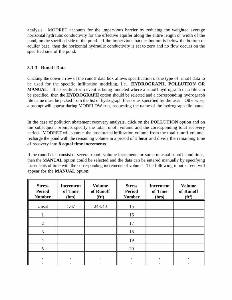
If the runoff data consist of several runoff volume increments or some unusual runoff conditions,then the MANUAL option could be selected and the data can be entered manually by specifyingincrements of time with the corresponding increments of volume. The following input screen willappear for the MANUAL option:

Stress Increment Volume Stress Increment VolumePeriod of Time of Runoff Period of Time of Runoff

Number (hrs) (ft ) Number (hrs) (ft )3 3

Unsat 1.67 243.40 15

1 16

2 17

3 18

4 19

5 20

. . . . . .

. . . . . .

On the first line prompt the program displays the calculated unsaturated infiltration time andvolume, if applicable, for review (in this case 1.67 hours and 243.4 ft ). The next 29 line3

prompts are available for input of incremental time (hrs) vs runoff volume (ft3). The user canspecify as many data pairs as necessary, but not more than a total of 29. For example, if the userdesires to specify only 3 or 4 points, the rest of the entry lines need not be filled in. Click on theOK button after input is completed. To create a graph for the model results, a minimum of twodata points must be specified for this option.

3.1.4 Overflow

Clicking the Overflow down-arrow allows selection of one of four options for overflow devicesof the pond, i.e., NONE, WEIR, ORIFICE & MANUAL. To select, click on the desiredoption. If NONE is selected, then the pond is modeled without overflow option. When WEIRoption is selected, it is necessary to select one of three types of typical weirs; V-notch, SharpCrested and Broad Crested. In the ORIFICE option, it is possible to specify any number ofsymmetrically identical orifices. The MANUAL option is provided to specify an overflow ratingdata set for overflow devices that do not fall into one of the other options. The manualspecification can also be used when a combination of different overflow devices are present, sinceit is not possible to utilize the weir and orifice options simultaneously.

The following weir data input screen prompt appears when WEIR - V_NOTCH option isspecified:

Weir Flow - Elevation vs Overflow Relationship

Structure Type: [ V_NOTCH – ] [ OK ]

Crest Elevation (ft): [ 0.00][ Cancel ]

Angle of “V” (degrees): [ 90.00]

Coefficient of Discharge: [ 2.50]

Weir Flow Exponent: [ 1.50]

Number of Contractions: [ 0.00]

Design High Water Level Elevation (ft) [ 3.00]

The Crest Elevation prompt allows specification of the actual elevation of the Vortex of theV_Notch weir. The Angle of “V” prompt allows specification of the angle (in degrees) of thev-notch of the weir. The Coefficient of Discharge "C" and the Weir Flow Exponent "a"prompts refer to parameters of the following weir equation:

Q = C tan(1/2) Ha

Where,Q = Flow rate (cfs)C = Coefficient of Discharge1 = Angle of V-Notch (degrees)H = Head on the weir (feet)a = Weir flow exponent

The Design High Water Elevation prompt appears here or below the Overflow selectionprompt, if NONE is selected. This prompt allows specification of the actual design high waterlevel or an estimated value (best guess). The purpose of specifying this value is to allowMODRET to develop a rating curve (to be used by MODFLOW) between the weir crest elevationand the design high water level (must always be > crest elevation). NOTE: This design highwater level data is also utilized by MODRET to calculate the average length and width of pond.This is done in combination with pond area of starting water level, pond volume and length towidth ratio data. Therefore, it is important to specify this value as accurately as possible. Thiselevation should always be correlated with the pond volume between starting water level andestimated high water level.

Once all weir input data prompts are answered, MODRET returns to the main data input screenand the Overflow option box is displayed with the selected overflow device. If a new weir deviceis selected at this point, the previously selected data will be ignored and prompts for a new set ofdata will appear.

The following weir data input screen prompt appears when WEIR - SHARP CRESTED orBROAD CRESTED option is selected:

Weir Flow - Elevation vs Overflow Relationship

Structure Type: [ SHARP CRESTED [– ] [ OK ]

Crest Elevation (ft): [ 0.00][ Cancel ]

Crest Length (ft): [ 1.00]

Coefficient of Discharge: [ 3.31]

Weir Flow Exponent: [ 1.50]

Number of Contractions: [ 0.00]

Design High Water Level Elevation (ft): [ 3.00]

The input prompts of Structure Type, Crest Elevation, Coefficient of Discharge, Weir FlowExponent and Design High Water Elevation are the same as presented for the V-Notch weir

option above.

The Crest Length prompt allows specification of the actual length of a rectangular sharp crestedor broad crested weir.

The Number of Contractions prompt allows specification of the number of weir end contractions(i.e., 0, 1 or 2). The following equation is used to calculate overflow over a sharp crested orbroad crested weir:

Q = C (L-0.1Hn)Ha

Where, Q = Flow rate (cfs)C = Coefficient of DischargeL = Crest length (feet)H = Head on the weir (feet)n = Number of weir end contractionsa = Weir flow exponent

General Conditions and Assumptions for Weir Flow Calculations

For ALL weir flow calculations it is assumed that the discharge is free flowing and is notsubmerged. It is assumed that the upstream water depth below the weir crest level is at least 2times the maximum head on the weir. For weir flows with end contractions it is assumed thatthe horizontal distance from the end of the weir crest to the side wall of the channel is at least 2times the maximum head on the weir.

The following data input screen appears when ORIFICE option is specified for the Overflowdevice:

Orifice - Elevation vs Overflow Relationship

Centerline Elevation of Orifice (ft) [ 0.00] [ OK ]

Area of Orifice (in ) [ 1.00] [ Cancel ]2

Coefficient of Discharge: [ 3.33]

Orifice Flow Exponent: [ 0.50]

Number of Identical Orifices: [ 1.00]

Design High Water Level Elevation (ft): [ 3.00]

The input parameters of Coefficient of Discharge, Orifice Flow Exponent, and Design HighWater Elevation are the same as presented for the Weir flow options above. However, the

coefficient of discharge in this equation is not the same as the coefficient of typical orificeequation. For MODRET the coefficient C = Co * (2g) The Centerline Elevation of Orifice0.5

prompt allows specification of the actual elevation of the centerline of a circular or symmetricalorifice to be modeled. The orifice is assumed to be unobstructed and without tailwatercondition. The Area of Orifice prompt allows specification of the total area (in inches squared)of individual orifice being specified. The Number of Identical Orifices prompt allowsspecification of the total number of identical orifices to be modeled, which must exist at the sameelevation and have the exact same size and flow conditions. The following equation is used tocalculate flow through the orifice:

Q = n C A Ha

Where, Q = Flow rate (cfs)n = Number of identical orificesC = Coefficient of Discharge [C=Co * (2g) , where Co = 0.6 to 0.9, typ.]0.5

A = Area of Orifice (ft )2

H = Head over the centerline of orifice (feet)a = Orifice flow exponent

The following data input screen appears when MANUAL option is specified for the Overflowdevice:

Manual - Elevation vs Overflow Relationship

Data Elevation Overflow Data Elevation OverflowPoint (ft) (cfd) Point (ft) (cfd)

Total Total

[ OK ]

1 0.00 13 [ Cancel ]

2 14

3 15

4 16

5 17

6 18

7 19

8 20

9 21

10 22

11 23

12 24

The data input for this option is typically referred to as the overflow rating curve method. Thefirst data point line prompts the user to specify only the elevation and a zero (0) is automaticallyassigned to the Total Overflow column. This indicates that the first entry must be the startingpoint of overflow (i.e, crest elevation of weir). Subsequent data point inputs have no restrictionof any kind. The user can specify as many data points as necessary, but not more than a totalof 24. For example, if the user only desires to specify 6 points, the rest of the entry lines neednot be filled in. The user must simply click on OK button after the 6th point data has beenspecified. When previously saved data is recalled for editing, the saved rating curve data will bedisplayed. To edit, simply over-write or add as needed. Elevation above the last input line willbe assumed equal to the last line entry.

3.1.5 File Management Control & Model Execution

On the top-right side of the infiltration input data screen, several command button are displayed.These include Run, Open, Save, Save As, Print and Cancel, see page 7. Once all the inputdata has been specified, the data should be saved by clicking on the Save or the Save As button. At this point the input data can be printed by clicking on the PRINT button. The PRINTcommand does allow a certain amount of print customization, such as portrait or landscape, papersize, printer selection, etc.. The Open option allows loading of an existing infiltration input datafile from the available list or a file name that can be specified by the user.

Once all the input data is specified and saved, the infiltration analysis can be executed by clickingon the Run button. The Run option allows creation of the MODFLOW files and execution ofthe MODFLOW model from within the MODRET program. It may take some time to executeMODFLOW, depending on the computer and the number of stress periods. A message box willappear indicating that MODFLOW is running. When execution of MODFLOW is complete, amessage will appear in the box, prompting the user to click OK to continue. If the MODFLOWmodel crashes during execution, an error message will appear in a message box.

3.1.6 Output

At the bottom-left corner of the infiltration input data screen four buttons appear, Input, View,Volume Infiltrated and Elevation of Water Level. Prior to selecting one of these options, theinfiltration analysis must be executed by clicking on the Run button.

Clicking on the Input button allows input and editing of the infiltration model input dataparameters. Clicking on the View button allows a tabular view of the infiltration model resultsand an option to print the tabular results by clicking on the Print button. Examples of theprintouts for the infiltration input data are included in Part 2 of this manual - Example Problems.

Clicking on the Volume Infiltrated button allows generation of a graphical view of the volume

infiltrated vs time. Clicking on the Elevation of Water Level button allows generation of agraphical view of the water elevation in the pond vs time. All displays of graphical results areprovided with a Print button to allow printing of the graphs. Examples of the graphical printoutsfor the model results are included in Part 2 of this manual - Example Problems.

3.2 Open...

Clicking on the Input/Graphic button, will display a list of input data file names that werepreviously created by MODRET. These have the extension ifl, however, other file extensioncan be specified by the user. To bring the input data files on the screen for review and editing,simply double click on the desired file name.

3.3 Delete...

Clicking on the Delete... button will display all the hydrograph input data files with the extensionifl. Double click on the file to be deleted and click on the Yes button. Other files with differentextensions can also be deleted by selecting the desired extension and file name.

4.0 Routing

The Routing module of MODRET allows routing of the runoff hydrograph through the retentionpond, subtracting infiltration losses, and creating a data file that contains six (6) sets of data withrespect to time of runoff. The six data sets can then be graphically displayed on the screen forreview and printout. Clicking on Routing will display the following box:

Create **

Load & Plot **

4.1 Create

Clicking on Create will display a file selection window for the runoff hydrograph to be routedthrough the retention pond. Simply select the appropriate hydrograph file and double click. Forrouting purposes, the latest pond infiltration analysis will be used to calculate the infiltration lossesfrom the pond with respect to time of runoff. If this routing run is for an existing set of datafiles, MODRET will compare the project names of the saved infiltration analysis data set and therouting analysis data set. If these do not match, an error message will appear indicating thediscrepancy of file names. After selection of the runoff hydrograph file, the following input boxwill appear:

Stage-Storage Data

Elevation Volume Volume(ft) (ft3) (ft3)

Pond PondElevation

(ft)

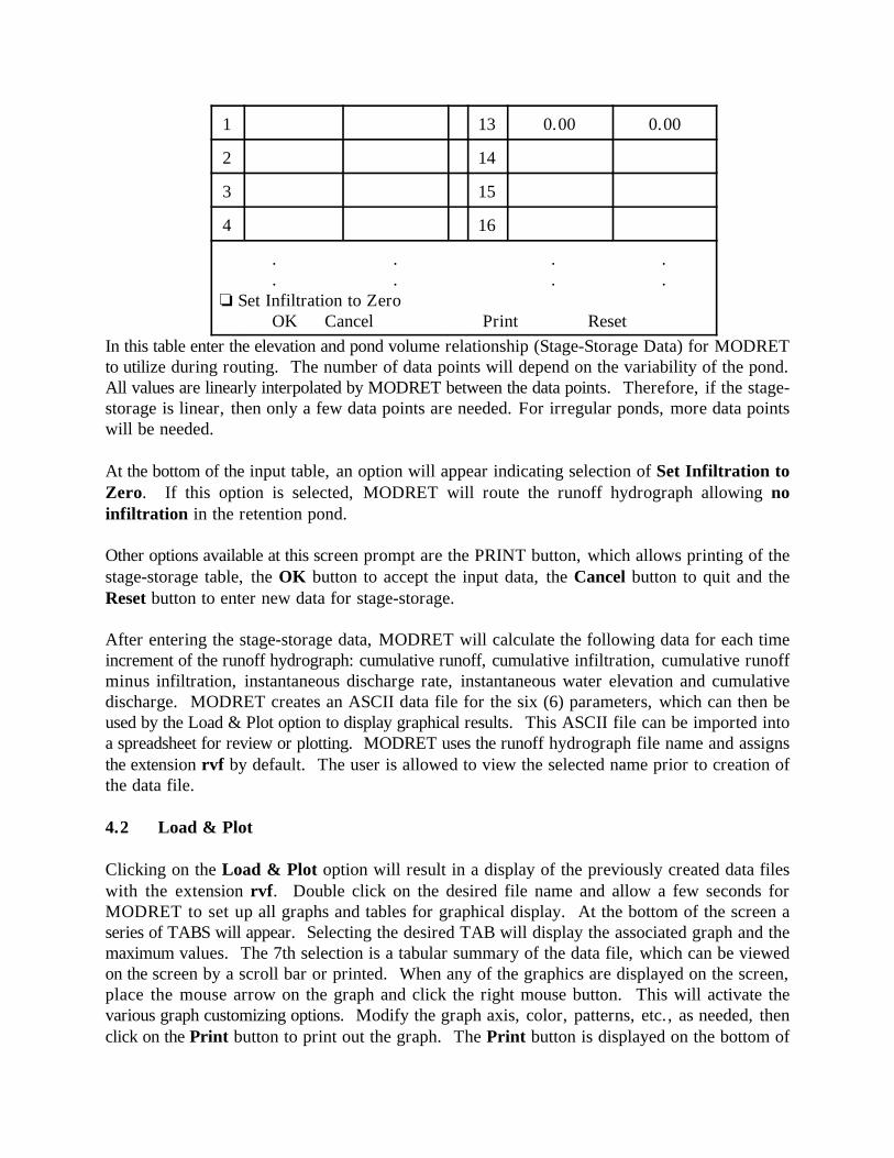
1 13 0.00 0.00

2 14

3 15

4 16

. . . .

. . . .‘ Set Infiltration to Zero

OK Cancel Print ResetIn this table enter the elevation and pond volume relationship (Stage-Storage Data) for MODRETto utilize during routing. The number of data points will depend on the variability of the pond.All values are linearly interpolated by MODRET between the data points. Therefore, if the stage-storage is linear, then only a few data points are needed. For irregular ponds, more data pointswill be needed.

At the bottom of the input table, an option will appear indicating selection of Set Infiltration toZero. If this option is selected, MODRET will route the runoff hydrograph allowing noinfiltration in the retention pond.

Other options available at this screen prompt are the PRINT button, which allows printing of thestage-storage table, the OK button to accept the input data, the Cancel button to quit and theReset button to enter new data for stage-storage.

After entering the stage-storage data, MODRET will calculate the following data for each timeincrement of the runoff hydrograph: cumulative runoff, cumulative infiltration, cumulative runoffminus infiltration, instantaneous discharge rate, instantaneous water elevation and cumulativedischarge. MODRET creates an ASCII data file for the six (6) parameters, which can then beused by the Load & Plot option to display graphical results. This ASCII file can be imported intoa spreadsheet for review or plotting. MODRET uses the runoff hydrograph file name and assignsthe extension rvf by default. The user is allowed to view the selected name prior to creation ofthe data file.

4.2 Load & Plot

Clicking on the Load & Plot option will result in a display of the previously created data fileswith the extension rvf. Double click on the desired file name and allow a few seconds forMODRET to set up all graphs and tables for graphical display. At the bottom of the screen aseries of TABS will appear. Selecting the desired TAB will display the associated graph and themaximum values. The 7th selection is a tabular summary of the data file, which can be viewedon the screen by a scroll bar or printed. When any of the graphics are displayed on the screen,place the mouse arrow on the graph and click the right mouse button. This will activate thevarious graph customizing options. Modify the graph axis, color, patterns, etc., as needed, thenclick on the Print button to print out the graph. The Print button is displayed on the bottom of

the graph. A typical routing graphics are included in Example 2, Part 2 of this document.

5.0 Graphic

The Graphic module of MODRET allows creation of various data files and graph files andgraphically plot the results for review and printout. Clicking on Graphic will display thefollowing box:

Create **

Load & Plot **

5.1 Create

The Create option allows generation of an XYZ data file of the groundwater/water elevationwithin the modeled grid for any time period modeled, a runoff-infiltration hydrograph data file,and a cross section graphic data file. Clicking on Create or hitting C will display the followingbox:

XYZ File...Runoff-Infiltration...Cross Section File...

The XYZ File option allows creation of an X (distance), Y (distance) and Z (groundwaterelevation) data file for any of the time periods modeled (1 hour, 12 hours, etc.). Selecting thisoption will result in a prompt to specify the desired File Name (without extension) to be createdand the approximate time of simulation. The model then selects the closest Stress Period modeledfor the XYZ file creation. Once the File Name and time are specified, the program calculatesall the distances, reads all the groundwater elevations of the entire 30 x 30 model grid system andgenerates an ASCII data file of XYZ, separated by spaces. This data file can then be importedinto a number of commercially available programs to generate groundwater contours or 3-dimensional view surfaces (i.e., SURFER , AutoCad , MathCad , and others).TM TM TM

The Runoff-Infiltration option allows regeneration of an existing runoff hydrograph by routingit through infiltration, from the latest executed MODRET data set. This option displays a box,prompting the user to select the runoff hydrograph file name (hydrograph to be routed). Doubleclick or select and click on OK button. The runoff-infiltration hydrograph file name will then beautomatically assigned by the program, which will have the same root name and an extensionof RHD and the file will be created. This runoff-infiltration hydrograph can then be usedwith any other surface routing models that do not have the capability to account forinfiltration losses.

The Cross Section File option allows creation of a data file which can then be plotted by the Load

& Plot option to display selected groundwater elevation cross sections along the X-axis and theY-axis of the retention pond. For this option, the program prompts the user to specify the FileName to be created, and the approximate Time of the model simulation. The model then selectsthe closest Stress Period modeled for the file creation. Note that MODRET uses the latestMODFLOW output file to create this data file. Therefore, this should be created immediatelyafter executing the infiltration model.

5.2 Load & Plot

Clicking on Load & Plot or hitting L will display the following box:

Cross Section

Clicking on Cross Section option will result in a display of cross sectional graphic files with theextension xsc. Double click on the desired file name or type in the desired name and extension,then click OK. This option allows a graphical display of various groundwater elevation crosssections through the pond and vicinity. On the top-right corner of the graph display the optionsof X-Axis and Y-Axis will appear. Select the desired cross section for display, i.e., X or Y.Directly below the X & Y option box, the corresponding distances in the perpendicular directionare summarized. Click on the down-arrow and select the desired distance of the Cross Sectionfor which viewing of groundwater level profile is desired. Alternatively, click on the window tothe left of the arrow and scroll through the cross sections using the up and down arrow keys.

The X-Axis runs along the width of the pond, starting at the center of the rectangular equivalentof the pond. Positive values are to the right and negative values are to the left of the center ofpond. The Y - Axis runs along the length of the pond, up and down, starting at the center of thepond. The positive numbers are to the top and the negative numbers are to the bottom. Selectionof one of these options will display a set of coordinate distances along the perpendicular axis tothe selected axis. The cross sectional distances from the pond center are selected by MODRET,based on the size of pond and groundwater control features. However, as a minimum there willbe a cross section through the center of pond and along the edges of pond. By selecting one ofthe distances, the corresponding groundwater cross section graphic will be generated. Typicalgroundwater cross sectional graphics are included in Examples 4 and 5, Part 2 of this user’sguide. A conceptualized pond within the model grid system and X, Y coordinates are presentedon Figure A-1 attached.

When the graphic is displayed on the screen, place the mouse arrow on the graph and click theright mouse button. This will activate the various graph customizing options. Modify the graphaxis, color, patterns, etc., as needed, then click on the Print button to print the graph.

6.0 Windows

The Windows option allows organization of the various working windows of the program and to

move from one file to another. The functions of the Windows is the same as for all windowsdriven programs.

7.0 ReadMe

Clicking on the ReadMe button will display the latest changes and upcoming upgrades to theMODRET model and other related comments and issues.