verification of randomized distributed algorithms under

HAL Id: hal-01925533https://hal.inria.fr/hal-01925533v2

Preprint submitted on 19 Nov 2018 (v2), last revised 19 Apr 2019 (v3)

HAL is a multi-disciplinary open accessarchive for the deposit and dissemination of sci-entific research documents, whether they are pub-lished or not. The documents may come fromteaching and research institutions in France orabroad, or from public or private research centers.

L’archive ouverte pluridisciplinaire HAL, estdestinée au dépôt et à la diffusion de documentsscientifiques de niveau recherche, publiés ou non,émanant des établissements d’enseignement et derecherche français ou étrangers, des laboratoirespublics ou privés.

Verification of Randomized Distributed Algorithmsunder Round-Rigid Adversaries

Nathalie Bertrand, Igor Konnov, Marijana Lazic, Josef Widder

To cite this version:Nathalie Bertrand, Igor Konnov, Marijana Lazic, Josef Widder. Verification of Randomized Dis-tributed Algorithms under Round-Rigid Adversaries. 2018. �hal-01925533v2�

https://hal.inria.fr/hal-01925533v2

https://hal.archives-ouvertes.fr

Verification of Randomized DistributedAlgorithms under Round-Rigid Adversaries ?

Nathalie Bertrand1, Igor Konnov2, Marijana Lazic3, and Josef Widder3

1 Inria Rennes, [email protected]

2 University of Lorraine, CNRS, Inria, LORIA, F-54000 Nancy, [email protected]

3 TU Wien (Vienna University of Technology), Vienna, Austria{lazic,widder}@forsyte.at

Abstract. Randomized fault-tolerant distributed algorithms pose a num-ber of challenges for automated verification: (i) parameterization in thenumber of processes and faults, (ii) randomized choices and probabilisticproperties, and (iii) an unbounded number of asynchronous rounds. Thecombination of these challenges makes verification hard. Challenge (i)was recently addressed in the framework of threshold automata.We extend threshold automata to model randomized algorithms that per-form an unbounded number of asynchronous rounds. For non-probabilisticproperties, we show that it is necessary and sufficient to verify these prop-erties under round-rigid schedules, that is, schedules where no processenters round r before all other processes finished round r−1. For almost-sure termination, we analyze these algorithms under round-rigid adver-saries, that is, fair adversaries that only generate round-rigid schedules.This allows us to do compositional and inductive reasoning that reducesverification of the asynchronous multi-round algorithms to model check-ing of a one-round threshold automaton.We apply this framework to classic algorithms: Ben-Or’s and Bracha’sseminal consensus algorithms for crashes and Byzantine faults, 2-setagreement for crash faults, and RS-Bosco for the Byzantine case.

1 Introduction

Fault-tolerant distributed algorithms is an active research area, and systems likePaxos and Blockchain receive much attention. These systems are out of reachwith current automated verification techniques. One problem comes from thescale: these systems should be verified for a very large number of participants,and even ideally for an unbounded number. In addition, many systems (includingBlockchain), provide probabilistic guarantees. To check their correctness, one hasto reason about randomized distributed algorithms in the parameterized setting.? Experiments presented in this paper were carried out using the Grid5000 testbed,

supported by a scientific interest group hosted by Inria and including CNRS, RE-NATER and several Universities as well as other organizations, see grid5000.fr.

2 Nathalie Bertrand, Igor Konnov, Marijana Lazic, and Josef Widder

1 Boolean v := input value2 Integer r := 13

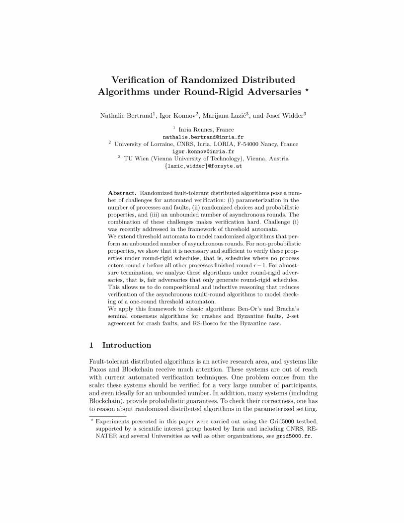
4 while (true) do5 send (R,r,v) to all;6

7 wait till received n − t messages (R,r,∗);8 if received (n + t) / 2 messages (R,r,w) have been received then9 send (P,r,w,D) to all

10 else11 send (P,r,?) to all;12

13 wait till received n − t messages (P,r,∗);14 if received at least t + 1 messages (P,r,w,D) then {15 v := w;16 if received at least (n + t) / 2 messages (P,r,w,D) then decide w }17 else v := 0 or 1 randomly18 r := r + 1

Fig. 1. Pseudo code of Ben-Or’s algorithm for Byzantine faults

In this paper, we make first steps towards parameterized verification of fault-tolerant randomized distributed algorithms. We consider the algorithms thatfollow the ideas of Ben-Or [2]. Interestingly, these algorithms were analyzedin [12,10] where probabilistic reasoning was done using the probabilistic modelchecker PRISM [11] for systems of 10-20 processes, while only safety was verifiedin the parameterized setting using Cadence SMV. From a different perspective,these algorithms extend asynchronous threshold-guarded distributed algorithmsfrom [8,7] with two features (i) a random choice (coin toss), and (ii) repeatedexecutions of the same algorithm until it converges (with probability 1).

A prominent example of a consensus algorithm is [2]. It circumvents the im-possibility of asynchronous consensus [5] by relaxing the termination requirementto almost-sure termination, i.e., termination with probability 1. This is achievedby a multi-round fault-tolerant distributed algorithm given in Figure 1. Hereprocesses execute an infinite sequence of asynchronous loop iterations, whichare called rounds r. Each round consists of two stages where they first exchangemessages tagged R, wait until the number of received messages reaches a cer-tain threshold (given as expression over parameters in line 7) and then exchangemessages tagged P . If n is the number of processes in the system, among whichat most t are faulty, then all the thresholds, that is, n− t and (n+ t)/2 and t+1,should ensure that no two correct processes ever decide on different values, evenif up to t Byzantine faulty processes send conflicting information. At the end ofa round, if there is no “strong majority” for a value, that is, (n+ t)/2 receivedmessages, a process picks a new value randomly in line 17.

While these complex threshold expressions can be dealt with using the meth-ods in [7], several challenges remain. Basically, the technique in [7] can be usedto verify one iteration of the round from Figure 1 only. However, consensusalgorithms should prevent that there are no two rounds r and r′ such that aprocess decides 0 in r and another decides 1 in r′. This calls for a compositionalapproach that allows one to compose verification results for individual rounds.A challenge in the composition is that distributed algorithms implement “asyn-chronous rounds”, that is, during the run processes may be in different roundsat the same time.

Verification of Randomized Distributed Algorithms 3

`0

`1

`2

`3

`4`5

`6

`7

r1

r2

r3 : x ≥ n− f 7→ y++

r4 : true 7→ x++

r5 : y ≥t

r7 r6 : y < t

12

12

Fig. 2. Example of a probabilistic threshold automaton.

In addition, the combination of distributed aspects and probabilities makesreasoning difficult. Quoting Lehmann and Rabin [13], “proofs of correctness forprobabilistic distributed systems are extremely slippery”. This advocates thedevelopment of automated verification techniques for probabilistic properties ofrandomized distributed algorithms in the parameterized setting.

Contributions. We lift threshold automata to round-based algorithms with cointoss transitions. For the new framework we achieve the following:

1. For safety verification we introduce a method for compositional round-basedreasoning. This allows us to invoke a reduction similar to the one in [4]. Wehighlight necessary fairness conditions on individual rounds. This providesus with specifications to be checked on a one-round automaton.

2. For probabilistic liveness verification, we explain how to reduce to provingtermination with positive probability within a fixed number of rounds. To doso, we justify the restriction to round-rigid adversaries, that is, adversariesthat respect the round ordering. In contrast to existing work that provesalmost-sure termination for fixed number of participants, these are the firstparameterized model checking results for probabilistic properties.

3. We checked the specifications that emerge from points 1. and 2. and thusverify challenging benchmarks in the parameterized setting. We verify Ben-Or’s [2] and Bracha’s [3] classic consensus algorithms, and the more recentalgorithms 2-set agreement [14], and RS-Bosco [16].

2 Overview

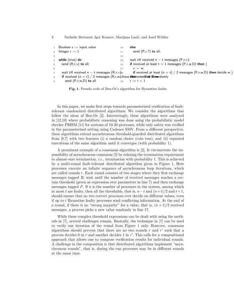
We introduce probabilistic threshold automata to model randomized threshold-based algorithms. An example of such an automaton is given in Figure 2. Nodesrepresent local states (or locations) of processes, which move along the labelededges or forks. Edges and forks are called rules. Labels have the form ϕ 7→ u,


meaning that a process can move along the edge only if ϕ evaluates to true, andthis is followed by the update u of shared variables. Additionally, each tine of afork is labeled with a number in the [0, 1] interval, representing the probabilityof a process moving along the fork to end up at the target location of the tine.

If we ignore the dashed arrows in Figure 2, a threshold automaton capturesthe behavior of a process in one round. The dashed edges, called round switchrules, encode how a process, after finishing a round, starts the next one. Sincein the algorithm from Figure 1 processes iterate through the rounds r and sendand receive messages for the round r, in the semantics of the automaton we willintroduce a copy of all variables (counters for locations and shared variables)for each round. Because there are infinitely many rounds, this means we haveinfinitely many variables.

Threshold automata without probabilistic forks and round switching rulescan be automatically checked for safety and liveness [7]. However, adding forksand round switches is required to adequately model randomized distributed al-gorithms.

In order to overcome the issue of infinitely many rounds, we prove in Section 5and Section 6 that we can verify probabilistic threshold automata by analyzinga one-round automaton, that fits in the framework of [7]. We prove that we canreorder transitions of any fair execution such that their round numbers are in anincreasing order. The obtained ordered execution is stutter equivalent with theoriginal one, and thus, they satisfy the same LTL-X properties over the atomicpropositions describing only one round. In other words, our targeted concurrentsystems can be transformed to a sequential composition of one-round systems.

The main problem with isolating a one-round system is that our specifica-tions often talk about at least two different rounds. In this case we need to useround invariants that imply the specifications. For example, if we want to ver-ify agreement, we have to check whether two processes decide different values,possibly in different rounds. We do this in two steps: (i) we check the roundinvariant that no process changes its decision from round to round, and (ii) wecheck that within a round no two processes disagree.

Finally, verifying almost-sure termination under round-rigid adversaries is innature very different from proving safety specification which are properties thatshould hold on every path, and involve no probabilities. It thus calls for distinctarguments. Our methodology follows the lines of the manual proof of Ben Or’sconsensus algorithm by Aguilera and Toueg [?]. However, our arguments arenot specific to Ben Or’s algorithm, and we apply it to other randomized dis-tributed algorithms (see Section 8). Compared to their paper-and-pencil proof,the threshold automata framework required us to provide a more formal settingand a more informative proof, also pinpointing the needed hypothesis. The cru-cial parts of our proof are automatically checked by the model checker ByMC.Hence the established correctness stands on less slippery ground, which addressesthe mentioned concerns of Lehmann and Rabin.


3 The Probabilistic Threshold Automata Framework

A probabilistic threshold automaton PTA is a tuple (L,V,R,RC ), where

– L is a finite set of locations, that contains the following disjoint subsets:initial locations I, final locations F , and border locations B, with |B| = |I|;

– V is a set of variables. It is partitioned in two sets: Π contains parametervariables, and Γ contains shared variables;

– R is a finite set of rules; and– RC , the resilience condition, is a formula in linear integer arithmetic over

parameter variables.

A rule r is a tuple (from, δto , ϕ,u) where from ∈ L is the source location,δto ∈ Dist(L) is a probability distribution over the destination locations, u ∈N|Γ |0 is the update vector, and ϕ is a guard of the form b · x ≥ a · pᵀ + a0 orb · x < a · pᵀ + a0, where x ∈ Γ is a shared variable, a ∈ Z|Π| is a vector ofintegers, a0, b ∈ Z, and p is the vector or all paremeters. If r.δto is a Diracdistribution, i.e., there exists ` ∈ L such that δto(`) = 1, we call r a Dirac rule,and sometimes write it as (from, `, ϕ,u). Destination locations of non-Dirac rulesare final locations.

Probabilistic threshold automata allow one to model algorithms with suc-cessive identical rounds. Informally, a round happens between border locationsand final locations, then round switch rules let processes move from final loca-tions of a given round to border locations of the next round. From each borderlocation there is exactly one Dirac rule to an initial location, and it has a form(`, `′, true,0) where ` ∈ B and `′ ∈ I. As |B| = |I|, one can think of borderlocations as copies of initial locations. It remains to model from which final loca-tions to which border location (that is, initial for the next round) processes move.This is done by round switch rules. These rules are deterministic, and can bedescribed by a function ρ : F → B, or equivalently as Dirac rules (`, `′, true,0)with ` ∈ F and `′ ∈ B. The set of round switch rules is denoted by S ⊆ R.

We assume the following structure for probabilistic threshold automata. Alocation is a border location if and only if all the incoming edges are round switchedges. Similarly, a location is final if and only if there is only one outgoing edgeand it is a round switch rule.

Example 1. In Figure 2 we have a PTA with border locations B = {`0, `1}, initiallocations I = {`2, `3}, and final locations F = {`5, `6, `7}. The only rule that isnot Dirac rule is r6, and round switch rules are represented by dashed arrows.

3.1 Probabilistic Counter Systems

Given a probabilistic threshold automaton PTA, we define its semantics, calledthe probabilistic counter system Sys(PTA), to be the infinite-state MDP (Σ, I,Act, ∆),where Σ is the set of configurations for PTA among which I ⊆ Σ are initial, theset of actions is Act = R × N0 and ∆ : Σ × Act → Dist(Σ) is the probabilistictransition function.


Every resilience condition RC defines the set of admissible parameters PRC ={p ∈ N|Π|0 : p |= RC}. We introduce a function N : PRC → N0 that maps avector of admissible parameters to a number of modeled processes in the system.

Configurations. Every configuration σ = (κ, g,p) is determined by a functionσ.κ : L×N0 → N0 that defines values of local state counters per round, a functionσ.g : Γ ×N0 → N0 defining shared variable values per round, and a vector σ.p ∈N|Π|0 of parameter values. By g[k] we denote the vector (g[x, k])x∈Γ of sharedvariables in a round k, and similarly by κ[k] we denote the vector (κ[`, k])`∈L oflocal state counters in a round k.

A configuration σ = (κ, g,p) is initial if for every x ∈ Γ and k ∈ N0 we haveσ.g[x, k] = 0, if

∑`∈B σ.κ[`, 0] = N(p), and finally if σ.κ[`, k] = 0, for every

(`, k) ∈ (L \ B)× {0} ∪ L × N.We say that a threshold guard ϕ : b · x ≥ a · pᵀ + a0 evaluates to true in a

configuration σ for a round k, and write σ, k |= ϕ, if b · σ.g[x, k] ≥ a · σ.pᵀ + a0.Similarly we define when a guard of the other form, that is, b · x < a · pᵀ + a0,evaluates to true in σ for a round k.

Actions. Actions are induced by the rules of PTA. They are of the form α =(r, k) ∈ R×N0 and stand for the application of rule r to some process4 in roundk. We use notation α.from for r.from, α.ϕ for r.ϕ, etc. If r is a Dirac rule, wesay α is a Dirac action.

An action α = (r, k) is unlocked in configuration σ, if its guard evaluatesto true in its round, that is σ, k |= ϕ. An action α = (r, k) is applicable to aconfiguration σ if α is unlocked in σ, and σ.κ[r.from, k] ≥ 1. Applicability thusrepresents the ability to apply r to σ in round k.

Definition 1. We introduce a partial function apply : Act × L × Σ 9 Σ suchthat given an action α = (r, k) ∈ Act, a location ` ∈ L, and a configuration σ, theresult apply(α, `, σ) is defined if and only if α is applicable to σ and α.δto(`) > 0.We have that apply(α, `, σ) = σ′ if and only if apply(α, `, σ) is defined and thefollowing holds:

– σ′.g[k] = σ.g[k] + α.u, and σ′.g[k′] = σ.g[k′], for every round k′ 6= k,– σ′.p = σ.p,– if r ∈ R \ S and α.from 6= `, then• σ′.κ[α.from, k] = σ.κ[α.from, k]− 1,• σ′.κ[`, k] = σ.κ[`, k] + 1,• ∀` ∈ L \ {α.from, `}, σ′.κ[`, k] = σ.κ[`, k], and• σ′.κ[k′] = σ.κ[k′], for all rounds k′ 6= k

if r ∈ R \ S and α.from = `, then σ′.κ = σ.κ,if r ∈ S, then• σ′.κ[α.from, k] = σ.κ[α.from, k]− 1,• σ′.κ[`, k + 1] = σ.κ[`, k + 1] + 1, and• σ′.κ[`′, k′] = σ.κ[`′, k′], for all (`′, k′) ∈ L×N0 \{(α.from, k), (`, k+ 1)}.

4 Note that actual id of the process is irrelevant.


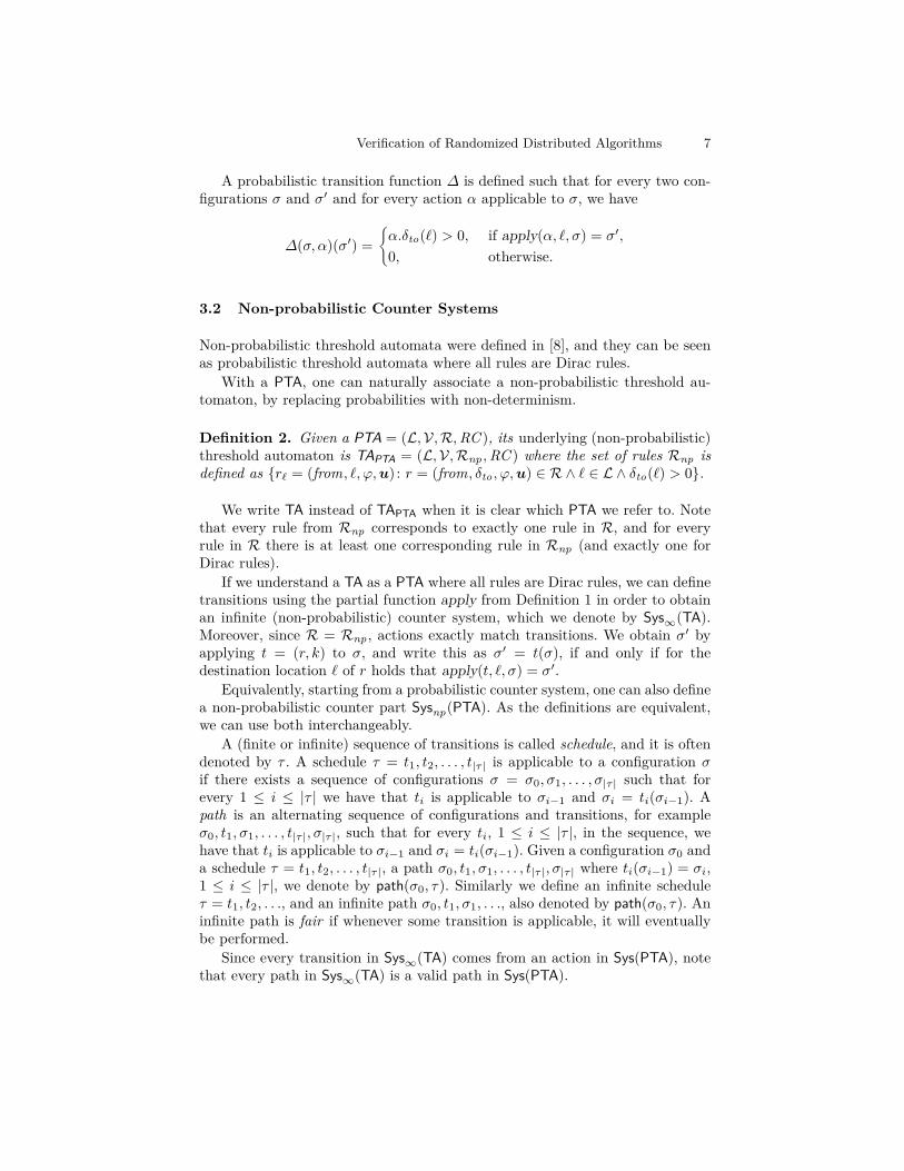
A probabilistic transition function ∆ is defined such that for every two con-figurations σ and σ′ and for every action α applicable to σ, we have

∆(σ, α)(σ′) =®α.δto(`) > 0, if apply(α, `, σ) = σ′,

0, otherwise.

3.2 Non-probabilistic Counter Systems

Non-probabilistic threshold automata were defined in [8], and they can be seenas probabilistic threshold automata where all rules are Dirac rules.

With a PTA, one can naturally associate a non-probabilistic threshold au-tomaton, by replacing probabilities with non-determinism.

Definition 2. Given a PTA = (L,V,R,RC ), its underlying (non-probabilistic)threshold automaton is TAPTA = (L,V,Rnp ,RC ) where the set of rules Rnp isdefined as {r` = (from, `, ϕ,u) : r = (from, δto , ϕ,u) ∈ R ∧ ` ∈ L ∧ δto(`) > 0}.

We write TA instead of TAPTA when it is clear which PTA we refer to. Notethat every rule from Rnp corresponds to exactly one rule in R, and for everyrule in R there is at least one corresponding rule in Rnp (and exactly one forDirac rules).

If we understand a TA as a PTA where all rules are Dirac rules, we can definetransitions using the partial function apply from Definition 1 in order to obtainan infinite (non-probabilistic) counter system, which we denote by Sys∞(TA).Moreover, since R = Rnp , actions exactly match transitions. We obtain σ′ byapplying t = (r, k) to σ, and write this as σ′ = t(σ), if and only if for thedestination location ` of r holds that apply(t, `, σ) = σ′.

Equivalently, starting from a probabilistic counter system, one can also definea non-probabilistic counter part Sysnp(PTA). As the definitions are equivalent,we can use both interchangeably.

A (finite or infinite) sequence of transitions is called schedule, and it is oftendenoted by τ . A schedule τ = t1, t2, . . . , t|τ | is applicable to a configuration σif there exists a sequence of configurations σ = σ0, σ1, . . . , σ|τ | such that forevery 1 ≤ i ≤ |τ | we have that ti is applicable to σi−1 and σi = ti(σi−1). Apath is an alternating sequence of configurations and transitions, for exampleσ0, t1, σ1, . . . , t|τ |, σ|τ |, such that for every ti, 1 ≤ i ≤ |τ |, in the sequence, wehave that ti is applicable to σi−1 and σi = ti(σi−1). Given a configuration σ0 anda schedule τ = t1, t2, . . . , t|τ |, a path σ0, t1, σ1, . . . , t|τ |, σ|τ | where ti(σi−1) = σi,1 ≤ i ≤ |τ |, we denote by path(σ0, τ). Similarly we define an infinite scheduleτ = t1, t2, . . ., and an infinite path σ0, t1, σ1, . . ., also denoted by path(σ0, τ). Aninfinite path is fair if whenever some transition is applicable, it will eventuallybe performed.

Since every transition in Sys∞(TA) comes from an action in Sys(PTA), notethat every path in Sys∞(TA) is a valid path in Sys(PTA).


3.3 Adversaries

Definition 3. Let Paths be the set of all finite paths in Sys(PTA). An adversaryis a function s : Paths→ Act, that given a path π selects an action applicable tothe last configuration of π.

Given a configuration σ and an adversary s, we generate a family of paths,depending of the outcomes of non-Dirac transitions. We denote this set bypaths(σ, s). An adversary s is fair if all paths in paths(σ, s) are fair.

As usual, the MDP Sys(PTA) together with an initial configuration σ and anadversary s induce a Markov chain, written Mσ

s . In the sequel, we write Pσs forthe probability measure over infinite paths starting at σ in the latter Markovchain.

Definition 4. An adversary s is round-rigid if it is fair, and if every sequenceof actions it produces can be written as s1 · sp1 · s2 · sp2..., where for every k ∈ N0,we have that sk contains only Dirac transitions of round k, and spk contains onlynon-Dirac transitions of round k.We denote the set of all round-rigid adversaries by AR.

3.4 Atomic Propositions and Stutter Equivalence

The atomic propositions we consider describe non-emptiness of the locationsfrom L \ B in a specific round. Formally, the set of all such propositions for around k ∈ N0 is denoted by APk = {p(`, k) : ` ∈ L \ B}. For every round k wedefine a labeling function λk : Σ → 2APk such that p(`, k) ∈ λk(σ) if and only ifσ.κ[`, k] > 0, i.e., if the location ` is nonempty in round k in σ.

For a path π = σ0, t1, σ1, . . . , tn, σn, n ∈ N, and a round k, a trace tracek(π)w.r.t. the labeling function λk is the sequence λk(σ0)λk(σ1) . . . λk(σn). Similarly,if a path is infinite π = σ0, t1, σ1, t2, σ2, . . ., then tracek(π) = λk(σ0)λk(σ1) . . ..

We say that two finite traces are stutter equivalent w.r.t. APk, denotedtracek(π1) , tracek(π2), if there is a finite sequence A0A1 . . . An ∈ (2APk )+,n ∈ N0, such that both tracek(π1) and tracek(π2) are contained in the languagegiven by the regular expression A+

0 A+1 . . . A

+n . If traces are of π1 and π2 are infi-

nite, then stutter equivalence tracek(π1) , tracek(π2) is defined in the standardway [1]. To simplify notation, we say that paths π1 and π2 are stutter equivalentw.r.t. APk, and write π1 ,k π2, instead of referring to specific path traces.

Two counter systems C0 and C1 are stutter equivalent w.r.t. APk, writtenC0 ,k C1, if for every path π from Ci there is a path π′ from C1−i such thatπ ,k π′, for i ∈ {0, 1}.

4 Consensus Properties and their Verification

Probabilistic consensus consists of safety specifications and an almost-sure ter-mination requirement. We discuss here the specifications of Ben-Or’s algorithmshown in Figure 1. Every correct process has an initial value from {0, 1}, andmust decide a value, either 0 or 1, such that:


Agreement: No two correct processes decide differently.Validity: If all correct processes have v as the initial value, then no process

decides 1− v.Probabilistic wait-free termination: Under every round-rigid adversary, with

probability 1 every correct process eventually decides.

Formalization. In order to formulate and analyze specifications, we partitionsets I, B, and F , each into two subsets, e.g., I0 and I1, and an analogous notationfor the subsets of B and F . Here are the restrictions for every v ∈ {0, 1}:

– Processes that are initially in a location ` ∈ Iv have the initial value v.– Rules connecting locations from B and I respect the partitioning, i.e., they

connect Bv and Iv.– Similarly, rules connecting locations from F and B respect the partitioning.

We also introduce two subsets Dv ⊆ Fv, for v ∈ {0, 1}. Intuitively, a process isin Dv in a round k if and only if it decides v in that round.

Now we can express specifications for Sys(PTA) as follows:

Agreement: For both values v ∈ {0, 1} holds the following:

(∀k ∈ N0)(∀k′ ∈ N0) A (F∨`∈Dv

κ[`, k] > 0 → G∧

`′∈D1−v

κ[`′, k′] = 0) (1)

Validity: For both v ∈ {0, 1} it holds

(∀k ∈ N0) A (∧`∈Iv

κ[`, 0] = 0 → G∧

`′∈Dv

κ[`′, k] = 0) (2)

Probabilistic wait-free termination: For every round-rigid adversary s

Ps( ∨k∈N0

∨v∈{0,1}

G∧

`∈F\Dv

κ[`, k] = 0)

= 1 (3)

Note that Agreement and Validity are non-probabilistic properties, and there-fore can be analyzed on Sys∞(TA) instead of Sys(PTA).

In Section 5 we formalize safety specifications and reduce them to single-round specifications. In Section 6 we reduce verification of single-round specifi-cations in the infinite counter system to their verification in a one-round countersystem. In Section 7 we discuss our approach to probabilistic termination.

5 Reduction to Specifications with one Round Quantifier

While Agreement contains two round variables, Validity talks about round 0 anda round k ∈ N0. Thus, both of these specifications involve two round numbers.Our goal is to reduce reasoning from unboundedly many rounds to one round.Therefore, properties are only allowed to talk about one round number. In thisSection we show how to check formulas (1) and (2) by checking properties that


describe one round. Namely, we introduce two properties, round invariants (4)and (5), and prove that they imply our two specifications.

Moreover, we define the Relay property, that is necessary for proving Proba-bilistic wait-free termination. Since this property also involves two round num-bers, we introduce another round invariant (16), and prove that together withformula (5) it implies Relay.

The first round invariant claims that in every round and in every path, oncea process decides v in a round, no process ever enters a location from F1−v inthat round. Formally written, we have the following:

(∀k ∈ N0) A (F∨`∈Dv

κ[`, k] > 0 → G∧

`′∈F1−v

κ[`′, k] = 0). (4)

The second round invariant claims that in every round in every path, if noprocess starts a round with a value v, then no process terminates that roundwith value v. Formally, the following formula holds:

(∀k ∈ N0) A (G∧`∈Iv

κ[`, k] = 0 → G∧`′∈Fv

κ[`′, k] = 0). (5)

The benefit of analyzing these two formulas instead of (1) and (2) lies in thefact that formulas (4) and (5) describe properties of only one round in a path,Next we want to prove that formulas (4) and (5) imply formulas (1) and (2).

Let us first give some useful properties of Sys∞(TA).

Lemma 1 (Round Switch). For every Sys∞(TA) and every v ∈ {0, 1}:

(∀k ∈ N0) A (G∧`∈Fv

κ[`, k] = 0 → G∧`′∈Iv

κ[`′, k + 1] = 0). (6)

Proof. By definitions of Fv, Bv and Iv, we have that

(∀k ∈ N0) A (G∧`∈Fv

κ[`, k] = 0→ G∧

`′′∈Bv

κ[`′′, k + 1] = 0), and

(∀k ∈ N0) A (G∧

`′′∈Bv

κ[`′′, k + 1] = 0→ G∧`′∈Iv

κ[`′, k + 1] = 0).

The two formulas together yield the required one for both values of v. ut

Lemma 2. For every Sys∞(TA) such that Sys∞(TA) |= (5), and for every v ∈{0, 1}, the following holds:

(∀k ∈ N0)(∀k′ ∈ N0)(k ≤ k′ → A (G

∧`∈Iv

κ[`, k] = 0→ G∧`′∈Iv

κ[`′, k′] = 0)),

(7)

(∀k ∈ N0)(∀k′ ∈ N0)(k ≤ k′ → A (G

∧`∈Fv

κ[`, k] = 0→ G∧`′∈Fv

κ[`′, k′] = 0)).

(8)


Proof. Assume formula (5) holds. Note that Lemma 1 together with formula (5)gives us that globally empty initial location is a round invariant. Formally, bytransitivity we have that

(∀k ∈ N0) A (G∧`∈Iv

κ[`, k] = 0 → G∧`′∈Iv

κ[`′, k + 1] = 0). (9)

By induction we obtain the required formula (7). Finally, by combining formu-las (6), (5) and (7) we obtain formula (8). ut

Proposition 1. If Sys∞(TA) |= (4) ∧ (5), then Sys∞(TA) |= (1) ∧ (2).

Proof. Assume Sys∞(TA) |= (4) ∧ (5).Let us first focus on formula (1), and prove that Sys∞(TA) |= (1). Assume by

contradiction that the formula does not hold on Sys∞(TA), that is, there existrounds k, k′ ∈ N0 and a path π such that:

π |= F∨

`0∈D0

κ[`0, k] > 0 ∧ F∨

`1∈D1

κ[`1, k′] > 0. (10)

Since by formula (10) we have π |= F∨`0∈D0

κ[`0, k] > 0, then from formula (4)with v = 0 we obtain that it also holds π |= G

∧`∈F1

κ[`, k] = 0. As D1 ⊆ F1,we know that no process decides 1 in round k. Now formula (8) from Lemma 2for v = 1 yields that π |= G

∧`∈F1

κ[`, k1] = 0 for every k1 ≥ k, i.e., in anyround greater than k no process will ever decide 1. As by (10) we have thatπ |= F

∨`1∈D1

κ[`1, k′] > 0, i.e., a process decides 1 in a round k′, thus it must

be that k′ < k.Now we consider the other part of formula (10), i.e., π |= F

∨`1∈D1

κ[`1, k′] >

0. By following the analogous analysis we conclude that it must be that k < k′.This brings us to the contradiction with k′ < k, which proves the first part ofthe statement, that violation of (4) and (5) implies violation of (1).

Next we focus on formula (2), and prove by contradiction that it must hold.We start by assuming that the formula does not hold, that is, there exists around k and a path π such that no process starts the first round of π withvalue v and eventually in a round k a process decides v. Formally,

π |=∧`∈Iv

κ[`, 0] = 0 ∧ F∨

`′∈Dv

κ[`′, k] > 0. (11)

Note first that π |=∧`∈Iv

κ[`, 0] = 0 implies π |= G∧`∈Iv

κ[`, 0] = 0.Then, since Sys∞(TA) |= (5), that is, since formula (5) holds, we have thatπ |= G

∧`′∈Fv

κ[`′, 0] = 0. Then by formula (8) we have that for every k ∈ N0it holds π |= G

∧`′∈Fv

κ[`′, k] = 0. Since Dv ⊆ Fv, we also have that π |=G∧`′∈Dv

κ[`′, k] = 0. As this contradicts our assumption from (11) that π |=F∨`′∈Dv

κ[`′, k] > 0, it proves the second part of the statement, that violationof (4) and (5) implies violation of (2). ut


6 Reduction to One-Round Counter System

Given a property describing one round, our goal is to prove that there is acounterexample to the property in the infinite system if and only if there is acounterexample in a one-round system. This is formulated in Theorem 1, and itallows us to use the existing technique from [7] on a one-round system.

The proof idea contains two parts. Firstly, in Section 6.1 we prove that onecan exchange an arbitrary finite schedule with a round-rigid one, while preservingatomic propositions of a fixed round. We show that swapping two neighboringtransitions that do not respect the order in an execution, gives us a legal stutterequivalent execution, i.e., an execution satisfying the same LTL-X properties.

Secondly, in Section 6.2 we extend this reasoning to infinite schedules, andlift it from schedules to transition systems. The main idea is to do inductive andcompositional reasoning over the rounds. In order to do so, we require that roundboundaries are well-defined, which is the case if every round that is started isalso finished; a property we can automatically check for fair schedules. In moredetail, regarding propositions for one round, we show in Lemma 11 that ourtargeted infinite transition system is stutter equivalent to a one-round transitionsystem. This holds under the assumption that all fair executions of a one-roundtransition system terminate, and this can be checked using the technique from [7].As stutter equivalence of systems implies preserving LTL-X properties, this isenough to prove the main goal of the section.

6.1 Reduction to round-rigid schedules

Definition 5. A schedule τ = (r1, k1) · (r2, k2) · . . . · (rm, km), m ∈ N0, is calledround-rigid if for every 1 ≤ i < j ≤ m, we have ki ≤ kj.

The following lemma follows directly from the definitions of transitions, andit gives us the most important transition invariants.

Lemma 3. Let σ be a configuration and let t = (r, k) be a transition. If σ′ = t(σ)then the following holds:

(a) σ′.g[k′] = σ.g[k′], for every round k′ 6= k,(b) σ′.κ[k′] = σ.κ[k′], for every round k′ ∈ N0 \ {k, k + 1},(c) σ′.κ[`, k′] = σ.κ[`, k′], for every round k′ 6= k and every location ` ∈ L \ B,(d) σ′.κ[k + 1] ≥ σ.κ[k + 1],

The following lemma establishes a central argument for inductive round-based reasoning: a transition belonging to a smaller round can always be movedbefore a transition of the larger round.

Lemma 4. Let σ be a configuration, and let t1 = (r1, k1) and t2 = (r2, k2) betransitions, such that k1 > k2. If t1 · t2 is applicable to σ, then t2 · t1 is alsoapplicable to σ.


Proof. Let us denote t1(σ) by σ1. As t1 · t2 is applicable to σ, this means that t1is applicable to σ and t2 is applicable to σ1. By definition of applicability, thismeans that

σ.κ[r1.from, k1] ≥ 1 and σ1.κ[r2.from, k2] ≥ 1, (12)

and additionally we have that σ, k1 |= t1.ϕ and σ1, k2 |= t2.ϕ.We show that t2 · t1 is applicable to σ by showing that: (i) t2 is applicable

to σ, and (ii) t1 is applicable to t2(σ).(i) First we need to show that σ.κ[r2.from, k2] ≥ 1 and σ, k2 |= t2.ϕ.As σ1 = t1(σ) and k2 < k1, by Lemma 3(b) we have σ1.κ[r2.from, k2] =

σ.κ[r2.from, k2]. From this and (12) we get that σ.κ[r2.from, k2] ≥ 1.Note that evaluation of the guard t2.ϕ depends only on the values of shared

variables σ.g[k2] in round k2 and parameter values σ.p. As σ1 = t1(σ) andk1 > k2, from Lemma 3(a) we have that σ.g[k2] = σ1.g[k2]. Recall that σ1, k2 |=t2.ϕ, and thus it must be the case that also σ, k2 |= t2.ϕ. This shows that t2 isapplicable to σ.

(ii) Let σ2 = t2(σ). Next we show that t1 is applicable to σ2. Using the samereasoning as in (i), we prove that σ2.κ[r1.from, k1] ≥ 1 and that σ2, k1 |= t1.ϕ.

As σ2 = t2(σ) and k2 < k1, Lemma 3(b) and 3(d) yield σ2.κ[r1.from, k1] ≥σ.κ[r1.from, k1]. Together with (12) we obtain that σ2.κ[r1.from, k1] ≥ 1.

To this end, we show that σ2, k1 |= t1.ϕ. Since σ2 = t2(σ) and k1 > k2, byLemma 3(a) we know that σ.g[k1] = σ2.g[k1]. Since by the initial assumption wehave σ, k1 |= t1.ϕ, and evaluation of the guard only depends on shared variablevalues and parameter values, then it also holds σ2, k1 |= t1.ϕ. ut

Lemma 5. Let σ be a configuration, let t1 = (r1, k1) and t2 = (r2, k2) be tran-sitions such that k1 > k2. If t1 · t2 is applicable to σ, then the following holds:

(a) Both t1 · t2 and t2 · t1 reach the same configuration, i.e., t1 · t2(σ) = t2 · t1(σ).(b) For every k ∈ N0 we have path(σ, t1 · t2) ,k path(σ, t2 · t1).

Proof. Note that since t1 · t2 is applicable to σ, we also have that t2 · t1 isapplicable to σ by Lemma 4, since k1 > k2.

(a) When a transition is applied to a configuration, the obtained configura-tion has the same parameter values, and counters and global variables are incre-mented or decremented depending on the transition (and independently of theinitial configuration). For any configuration (κ, g,p), we can write ti(κ, g,p) =(κ+ ui, g + vi,p) for i ∈ {1, 2}, and some vectors u1,u2,v1,v2 of integers. Byonly using commutativity of addition and subtraction, we obtain t1 · t2(σ) =(κ+ u1 + u2, g + v1 + v2,p) = (κ+ u2 + u1, g + v2 + v1,p) = t2 · t1(σ).

(b) Let σ1 = t1(σ), let σ2 = t2(σ), and σ3 = t1 ·t2(σ). Then tracek(path(σ, t1 ·t2)) = λk(σ)λk(σ1)λk(σ3), and tracek(path(σ, t2 · t1)) = λk(σ)λk(σ2)λk(σ3). Weconsider three cases: (i) k 6= k1 and k 6= k2, (ii) k = k1, and (iii) k = k2.(i) In this case, by Lemma 3(c), we have λk(σ) = λk(σ1) = λk(σ2) = λk(σ3).Thus, both traces are λk(σ)λk(σ)λk(σ), and they are clearly stutter equivalent.


(ii) Since k = k1 > k2, then again by Lemma 3(c) we have that λk(σ1) = λk(σ3)and λk(σ) = λk(σ2). Thus, tracek(path(σ, t1 · t2)) = λk(σ)λk(σ3)λk(σ3), andtracek(path(σ, t2 ·t1)) = λk(σ)λk(σ)λk(σ3), and the traces are stutter equivalent.(iii) The last case is analogous to the previous one. ut

The following lemma tells us that adding or removing transitions of a rounddifferent from k results in a k-stutter equivalent path.

Lemma 6. Let σ be a configuration and let t1 = (r1, k1) and t2 = (r2, k2) betransitions such that t1t2 is appllicable to σ. Then the following holds:

(a) path(σ, t1t2) ,k path(σ, t1), for every k 6= k2, and(b) path(σ, t1t2) ,k path(t1(σ), t2), for every k 6= k1.

Proof. It follows directly from Lemma 3 (c). ut

The following reduction theorem shows that every schedule can be re-orderedinto a round-rigid schedule that for all rounds k is stutter equivalent regardingLTL-X formulas over proposition over k.

Proposition 2. For every configuration σ and every finite schedule τ applicableto it, there is a round-rigid schedule τ ′ such that the following holds:

(a) Schedule τ ′ is applicable to σ.(b) τ ′ and τ reach the same configuration when applied to σ, i.e., τ ′(σ) = τ(σ).(c) For every k ∈ N0 we have path(σ, τ) ,k path(σ, τ ′).

Proof. Since τ is finite, the claim (a) follows from Lemma 4, the second claimfollows from Lemma 5(a), and the last one from Lemma 5(b). ut

The following proposition follows from the well-known result that stutterequivalent traces satisfy the same LTL-X specifications [1, Thm. 7.92].

Proposition 3. Fix a k ∈ N0. If π1 and π2 are paths such that π1 ,k π2, thenfor every formula ϕ from LTL-X over APk we have π1 |= ϕ if and only if π2 |= ϕ.

We conclude that instead of reasoning about all schedules of Sys∞(TA), it isthus sufficient to reason about its round-rigid schedules. In the following sectionwe will use this to simplify the verification further, namely to a one-round countersystem.

6.2 From round-rigid schedules to one-round counter system

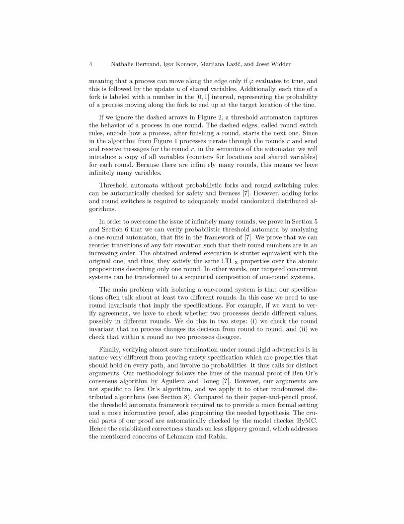
For each PTA, we define a round threshold automaton that can be analyzed withthe tools of [8] and [7]. Roughly speaking, we focus on one round, but also keepthe border locations of the next round, where we add self-loops. We show thatfor specific fairness constraints, this automaton shows the same behavior as around in Sys∞(TA). In Theorem 1 we prove that we can use it for analysis ofnon-probabilistic properties of Sys∞(TA).


`0

`1

`2

`3

`4`5

`6

`7

r1

r2

r3 : x ≥ n− f 7→ y++

r4 : true 7→ x++

r5 : y ≥t

r7

r6,`6 : y < t

r6,`7 : y < t

`′0

`′1

r8

r9

r10

r11

r12

Fig. 3. The TArd obtained from PTA in Figure 2

In the proof we restrict ourselves to fair schedules, that is, those where everytransition that is applicable will eventually be performed. We also assume thatevery fair schedule of a one-round algorithm terminates. Under the fairness as-sumption we check the latter assumption with ByMC [9]. Moreover, we restrictourselves to deadlock-free threshold automata, that is, we require that in eachconfiguration each location has at least one outgoing edge unlocked. As we useTAs to model distributed algorithms, this is no restriction: locations in whichno progress should be made unless certain thresholds are reached, typically haveself-loops that are guarded with true. Thus for our benchmarks one can easilycheck whether they are deadlock-free using SMT.

Definition 6. Given a PTA = (L,V,R,RC ) or its TA = (L,V,Rnp ,RC ), wedefine a round threshold automaton TArd to be the tuple (L ∪ B′,V,Rrd,RC ),where B′ = {`′ : ` ∈ B} are copies of border locations, and Rrd is defined asfollows. We have Rrd = (Rnp \ S)∪ S ′ ∪Rloop, where modifications S ′ of roundswitch rules are

S ′ = {(from, `′, true,0) : (from, `, true,0) ∈ S with `′ ∈ B′},

and Rloop = {(`′, `′, true,0) : `′ ∈ B′} are self-looping rules at locations from B′.Initial locations of TArd are locations from B ⊆ L.

For a TArd and a k ∈ N0 we define a counter system Sysk(TArd) as the tu-ple (Σk, Ik, Rk): A configuration is a tuple σ = (κ, g,p) ∈ Σk, where σ.κ : D →N0 defines values of the counters, for D = (L × {k}) ∪ (B′ × {k + 1}); andσ.g : Γ × {k} → N0 defines shared variable values; and σ.p ∈ N|Π|0 is a vector ofparameter values.

Note that by the definition of σ.κ usingD, every configuration σ ∈ Sysk(TArd)can be extended to a valid configuration of Sys∞(TA), by assigning values ofall other counters and global variables to zero. In the following, we identify aconfiguration in Sysk(TArd) with its extension in Sys∞(TA), since they have thesame labeling function λk, for every k ∈ N0.

We define ΣkB ⊆ Σk, for a k ∈ N0, to be the set of all configurations σ such

that σ.g[x, k] = 0 for all x ∈ Γ , then∑`∈B σ.κ[`, k] = N(p), and σ.κ[`, i] = 0

for all (`, i) ∈ D \ (B × {k}). We call these configurations border configurationsfor the round k. The set of initial states Ik is a subset of Σk

B.


We define the transition relation R as in Sys∞(TA), i.e., two configurationsare in the relation Rk if and only if they (or more precisely, their above describedextensions) are in R.

If we do not restrict initial configurations, all these systems are isomorphic,and this is formalized in the following Lemma.

Lemma 7. All systems Sysk(TArd), k ∈ N0, are isomorphic to each other w.r.t.ΣkB, i.e., for every k ∈ N0, if Ik = Σk

B, then we have Sys0(TArd) ∼= Sysk(TArd).

We restrict our attention to fair paths, that is, those paths π such thatfor every configuration σ in π the following holds: if a transition is applicable,then it will eventually be fired in π. Moreover, we assume that all such pathsin Sys0(TArd) terminate, that is, they reach a configuration with all processesin B′. Formally, we assume that for every fair path π in Sys0(TArd) it holds thatπ |= F

∧`∈L κ[`, 0] = 0. This can easily be checked with ByMC [9].

Lemma 8. If all fair executions in Sys0(TArd) terminate w.r.t. Σ0B, then the

same holds for Sysk(TArd) w.r.t. ΣkB, for every k ∈ N0.

Proof. It follows directly from Lemma 7. ut

We assume that in TA (and thus also in TArd) holds that for every config-uration, every location, and every round, there is an unlocked outgoing edgefrom ` in that configuration and that round. Formally, for every σ, `, and k,there is a rule r such that r.from = ` and σ, k |= r.ϕ. This property assures thatsystems Sys∞(TA) and Sysk(TArd), k ∈ N0, are deadlock-free.

In order to relate Sys∞(TA) and Sysk(TArd), k ∈ N0, we define the set ofinitial states I0 of Sys0(TArd) to be the set I of initial states of Sys∞(TA), andthen inductively we define Ik+1 to be the set of final configurations of Sysk(TArd).

From now on, we fix a TA and a TArd, and if not specified differently, forevery Sysk(TArd) we assume the above definition of Ik.

Lemma 9. If all fair executions of Sys0(TArd) w.r.t. Σ0B terminate, then for

every k ∈ N0 we have that the set Ik is well-defined and all fair executionsof Sysk(TArd) terminate (w.r.t. Ik).

Proof. We prove this claim by induction on k ∈ N0. The set I0 = I is clearly well-defined, and since I0 ⊆ Σ0

B, by our assumption we have that all fair executionsof Sys0(TArd) terminate. Since for every k ∈ N0 we have Ik ⊆ Σk

B, by Lemma 8we have that every fair execution of Sysk(TArd) terminates and therefore Ik+1

is well-defined. ut

Let us make here a short digression by giving a property of every Sys∞(TA),which is necessary for proving Lemma 11.

Lemma 10. Let Sys∞(TA) be deadlock-free, fix a k ∈ N0 and let σ be a con-figuration in Sys∞(TA) with a non-empty border location in round k + 1, i.e.,∨`∈B σ.κ[`, k + 1] ≥ 1. Then for every configuration σ′ reachable from σ, there

is a transition t = (r, f, k1) with k1 > k that is applicable to σ′.


Proof. Let σ be a configuration with a non-empty border location in round k+1,and let σ′ be a configuration reachable from σ. Assume by contradiction thatthere is no transition t = (r, f, k1) with k1 > k that is applicable to σ′. Recall thatevery location has a non-guarded outgoing rule. Thus, it must hold that for everylocation ` we have that σ′.κ[`, k1] = 0, for every k1 > k. This is a contradictionwith the assumption that σ′ is reachable from σ and

∨`∈B σ.κ[`, k + 1] ≥ 1. ut

Lemma 11. If Sys∞(TA) is deadlock-free, and if all fair executions of Sys0(TArd)w.r.t. Σ0

B terminate, then for every k ∈ N0 we have Sysk(TArd) ,k Sys∞(TA),i.e., the two systems are stutter equivalent w.r.t. APk.

Proof. We prove the statement by induction on k ∈ N0.Base case. Let us first show that Sys0(TArd) ,0 Sys∞(TA)(⇒) Let π = path(σ, τ) be a path in Sys0(TArd). We need to find a path π′

from Sys∞(TA), such that π ,k π′.If τ = t1t2 . . ., then every transition ti either exists also in TA, or it is a

self-loop at the copy of a border location. Using this, we construct a scheduleτ ′ = t′1t

′2 . . . in the following way.

For every i ∈ N, if ti exists in TA, then we define t′i to be exactly ti, and if t′i isa self-loop at an `′ ∈ B′, then Lemma 10 gives us that there exists a transition tifrom a round greater than 0 that is applicable to the current configuration, andwe define t′i = ti. Thus, τ ′ = t′1t

′2 . . . is obtained from τ by removing certain self-

looping transitions and adding transitions of rounds greater than 0. By Lemma 6we have path(σ, τ ′) ,0 path(σ, τ).

Now we have that π′ = path(σ, τ ′) ,0 path(σ, τ) = π.(⇐) Let now π = path(σ, τ) be a path in Sys∞(TA). We construct a path π′ =

path(σ′, τ ′) from Sysk(TArd) such that π ,k π′. Since I = I0, we define σ′ = σ.Let τ0 be the projection of τ to round 0. There are two cases to consider. First,

if τ and τ0 are either both infinite or both finite schedules, then by Lemma 6 theyyield stutter equivalent paths starting in σ. Observe that by Lemma 3 countersκ[`, 0] only change due to transitions for round 0, so that the applicability ofτ0 to σ follows from the applicability of τ .. Thus, in these cases we define τ ′ tobe τ0.

Second, we show the construction of τ ′ in the case when τ is an infiniteschedule and τ0 is finite. In this case we construct τ ′ as infinite extension ofτ0 as follows: Note that, since TA is deadlock-free, there must exist at least onelocation ` ∈ B1 that is nonempty after executing τ0 from σ, i.e., τ0(σ).κ[`, 1] ≥ 1.This must also be the case in Sys0(TArd), with a difference that the nonemptylocation belongs to B′, since B′ plays the role of B1. If r is the self-loopingrule at `, then we obtain τ ′ by concatenating infinitely many transitions (r, 1)to τ0, i.e., τ ′ = τ0(r, 1)ω. Transition (r, 1) does not affect atomic propositions ofround 0, and thus we have stutter equivalence by Lemma 6.

Induction step. Assume that Sysi(TArd) ,i Sys∞(TA) for every 0 ≤ i < k,and let us prove that the claim holds for k.

(⇒) Let π = path(σ, τ) be a path in Sysk(TArd). We need to find a path π′

from Sys∞(TA), such that π ,k π′.


First note that σ ∈ Ik. By definition of Ik, there exist a configuration σ0 ∈ I0

and schedules τ1, τ2, . . . , τk−1, such that every τi contains only transitions fromround i, and τ1τ2 . . . τk−1(σ0) = σ. Since no transition here is from round k, byLemma 6 we have that path(σ0, τ1τ2 . . . τk−1) ,k path(σ, ε), where ε is the emptyschedule. This path will be a prefix of π′.

If τ = t1t2 . . ., then we use the same strategy as in the base case to defineτ ′ = t′1t

′2 . . . such that path(σ, τ ′) ,k path(σ, τ).

Now we have that π′ = path(σ0, τ1τ2 . . . τk−1τ′) ,k path(σ, ετ) = π.

(⇐) Let now π = path(σ, τ) be a path in Sys∞(TA). We construct a path π′

from Sysk(TArd) such that π ,k π′.Since we assume that all fair executions of Sys0(TArd) terminate w.r.t. Σ0

B,then by Lemma 9 for every 0 ≤ i < k the set Ii is well-defined and all fairexecutions of Sysi(TArd) terminate. By the induction hypothesis, we know thatSysi(TArd) ,i Sys∞(TA). Together, this gives us that all rounds i, with 0 ≤ i < k,terminate in Sys∞(TA). In other words, every execution of Sys∞(TA) has a finiteprefix that contains all its transitions of rounds less than k.

Let τpre be such a prefix of τ = τpreτsuf. Because τpre is finite, we may invokeProposition 2, from which follows that there exist schedules τ0, τ1, . . . , τk−1, τ≥ksuch that every τi, 0 ≤ i < k contains only round i transitions, τ≥k containstransitions of rounds at least k, the schedule τ0τ1 . . . τk−1τ≥k is applicable to σ,leads to τpre(σ) when applied to σ, and

path(σ, τ0τ1 . . . τk−1τ≥kτsuf) ,k path(σ, τpreτsuf). (13)

Since σ ∈ I = I0, the existence of schedules τ0, τ1, . . . , τk−1 confirms thatσ′ = τ0τ1 . . . τk−1(σ) is in Ik. Next we apply the strategy from the base case toconstruct τ ′ from τ≥kτsuf, by projecting it to round k, such that

path(σ′, τ≥kτsuf) ,k path(σ′, τ ′). (14)

By (13) and (14) we get π′ = path(σ, τ0τ1 . . . τk−1τ′) ,k path(σ, τpreτsuf) = π.

ut

By Lemma 7, for every k ∈ N0 and every σ ∈ ΣkB, there is a corresponding

configuration σ′ ∈ Σ0B obtained from σ by renaming the round k to 0. Let fk be

the renaming function, i.e., σ′ = fk(σ). Let us define Σu ⊆ Σ0B to be the union

of all renamed initial configurations {fk(σ) : k ∈ N0, σ ∈ Ik}.

Theorem 1. Let system Sys∞(TA) be deadlock-free, and let all fair executionsof Sys0(TArd) w.r.t. Σ0

B terminate. Given a formula ϕ[i] from LTL-X over APi, fora round variable i, we have Sys0(TArd) |= Eϕ[0] w.r.t. initial configurations Σu

if and only if there exists a k ∈ N0 such that Sys∞(TA) |= Eϕ[k].

Proof. Let us first assume that Sys0(TArd) |= Eϕ0 w.r.t. initial configura-tions Σu. This means there is a path π = path(σ, τ) such that σ ∈ Σu andπ |= ϕ0. Since σ ∈ Σu, there is a k ∈ N0 and a σk ∈ Ik such that σ = fk(σk).From Lemma 7 we know that Sys0(TArd) ∼= Sysk(TArd), and thus there is a


schedule τk in Sysk(TArd) such that path(σk, τk) |= ϕk. Now Lemma 11 tells usthat there must be a path π′ from Sys∞(TA) such that path(σk, τk) ,k π′. ByProposition 3 we know that π′ |= ϕk, and thus Sys∞(TA) |= Eϕk. This provesone direction of the statement.

Assume now that there is a k ∈ N0 such that Sys∞(TA) |= Eϕk. Thus,there is a path π = path(σ, τ) in Sys∞(TA) such that π |= ϕk. By Lemma 11we know that there is a path π′ = path(σ′, τ ′) in Sysk(TArd) with π ,k π′, andthen by Proposition 3 also π′ |= ϕk. Finally, by Lemma 7 there is an equivalentpath π0 in Sys0(TArd) starting in fk(σ′). Then we have that π0 |= ϕ0, and sincefk(σ′) ∈ Σu, we know that Sys0(TArd) |= Eϕ0 w.r.t. initial configurations Σu.This concludes the other direction of the proof. ut

In Section 4 we show how to reduce our specifications to formulas of the form(∀k ∈ N0)Aψ[k]. Theorem 1 deals with negations of such forms, namely withexistence of a round k such that formula Eϕ[k] holds. Therefore, the theoremallows us to check on the one-round system instead of on the infinite one, if thereis a counterexample to formulas we want to check.

7 Probabilistic Wait-Free Termination

We start by introducing two sufficient conditions for Probabilistic Wait-FreeTermination under round-rigid adversaries. This is formalized in Theorem 2.

One condition is the existence of a positive probability lower-bound for acertain event to happen, that is, Theorem 2(a). In order to verify it, we reduceit in two steps to the form that ByMC is able to check. First, in Section 7.1 wereduce it to a non-probabilistic condition, which unfortunately is not in a conve-nient form. Second, in Section 7.2 we modify the system to a non-probabilisticone, and modify the condition to the convenient form (∀k ∈ N0) Aϕ[k] on thenew system.

The other condition, Theorem 2(b), already has the correct form, and canbe checked on ByMC without modifying the system and the formula.

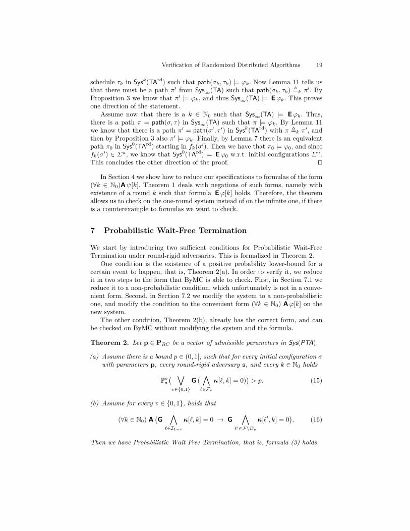
Theorem 2. Let p ∈ PRC be a vector of admissible parameters in Sys(PTA).

(a) Assume there is a bound p ∈ (0, 1], such that for every initial configuration σwith parameters p, every round-rigid adversary s, and every k ∈ N0 holds

Pσs( ∨v∈{0,1}

G (∧`∈Fv

κ[`, k] = 0))> p. (15)

(b) Assume for every v ∈ {0, 1}, holds that

(∀k ∈ N0) A(G

∧`∈I1−v

κ[`, k] = 0 → G∧

`′∈F\Dv

κ[`′, k] = 0). (16)

Then we have Probabilistic Wait-Free Termination, that is, formula (3) holds.


Proof. Fix a p ∈ PRC , an initial configuration σ0, and a round-rigid adversary s.Assume there is a non-zero probability p such that from any initial configura-tion σ over p and under any round-rigid adversary s formula (15) holds.

Two options may occur along a path π ∈ paths(σ0, s): (i) either round 0 endswith a final configuration in which all processes have the same value, say v, or(ii) round 0 ends with a final configuration with both values present.

(i) In this case we have that π |= G (∧`∈F1−v

κ[`, 0] = 0), and by our as-sumption, i.e., formula (15) for k = 0, the probability that this case happensis at least p. Then, by Lemma 1 we also have π |= G (

∧`∈I1−v

κ[`, 1] = 0). Byformula (16), in this case all processes decide value v in round 1.

(ii) The probability that the second case happens is at most 1 − p. In thiscase, round 1 starts with an initial configuration σ1 with both initial values 0and 1. From σ1 under s, by the same reasoning as from σ0, at the end on theround 1 we have the analogous two cases, and all processes decide in round 2with probability at least p.

Iterating this reasoning, almost surely all processes eventually decide. Let usformally explain this iteration. Let σ0 be an initial configuration, and let s be around-rigid adversary. For a k ∈ N, consider the event Ek: from σ0 and under s,not every process decides in the first k rounds. In particular, at the end of everyround i < k it is not the case that everyone decides. By the reasoning above,namely case (ii) for round i, this happens with probability at most (1 − p).Therefore, for k rounds we have Pσs (Ek) ≤ (1 − p)k. The limit when k tendsto infinity yields that the probability for not having Probabilistic Wait-FreeTermination is 0. This is equivalent to the required formula (3). ut

7.1 Reduction to one-round non-probabilistic specificationWe have previously used the idea of decomposing an infinite counter systemSys∞(TA) into one-round systems Sysk(TArd). In Sys(PTA), this idea is even morestraightforward since we consider only round-rigid adversaries. They guaranteethat rounds are ordered in all generated paths.

Since the assumption (a) in Theorem 2 is a property of one-round k inthe whole system Sys(PTA), we introduce analogous objects as in the non-probabilistic case. Namely, we introduce a PTArd (analogously as in Defini-tion 6), and its counter system Sysk(PTArd), for every k ∈ N0. Initial config-urations of Sysk(PTArd) are denoted by Ik (as they do coincide, similarly to thenon-probabilistic case). Moreover, for a fixed vector of parameters p, the set ofconfigurations σ from Ik with σ.p = p is denoted by Ikp.

Now, instead of checking that Theorem 2(a) holds on Sys(PTA), since theproperty itself refers only to one round k, it can be checked on the one-roundsystem Sysk(PTArd) as in Lemma 12(a).

In the following lemma we explain how to use non-probabilistic reasoning inorder to prove a probabilistic property.Lemma 12. Let k ∈ N0 and let p ∈ PRC be a parameter valuation in Sysk(PTArd).For every LTL formula ϕ[k] over atomic proposition APk of round k, the follow-ing three formulas are equivalent:


(a) (∃p > 0) (∀σ ∈ Ikp) (∀s ∈ AR) Pσs(ϕ[k]

)> p,

(b) (∀σ ∈ Ikp) (∀s ∈ AR) Pσs(ϕ[k]

)> 0,

(c) (∀σ ∈ Ikp) (∀s ∈ AR) (∃π ∈ paths(σ, s)) π |= ϕ[k].

Proof. Fix parameters p ∈ PRC .The two implications from top to bottom are trivial: if a probability is lower

bounded by a positive constant, then it is positive; and if the probability of agiven property is positive, then there must be at least a path satisfying thatproperty. It is thus sufficient to prove that the last statement implies the firstone to obtain all equivalences.

Assume that from all initial configuration σ with parameter values p, andunder all round-rigid adversaries s, there exists a path π ∈ paths(σ, s) such thatπ |= ϕ[k]. Observe that, independently of σ and s, since there are no cyclesin PTA, and since PTA contains a fixed number c of non-Dirac transitions, wehave that for any path, the prefix corresponding to round 0 has at most c ·N(p)non-Dirac transitions. The probability of the set of all infinite paths that havethe same prefix of round 0 as π, is thus at least 2−c·N(p). Therefore, we candefine a positive probability p = 2−c·N(p) to be our lower bound, which onlydepends on PTA and p such that, in Sys(PTArd) we have that (∃p > 0)(∀σ ∈Ikp)(∀s ∈ AR) Pσs

(ϕ[k]

)> p. This concludes the proof. ut

The following Corollary shows how to apply Lemma 12 to the property weneed in Theorem 2.

Corollary 1. The assumption (a) from Theorem 2 is equivalent to the following:for every k ∈ N0 in Sysk(PTArd) holds that for every vector of parameters p ∈PRC , for every initial configuration σ ∈ Ikp, and for every round-rigid adversarys, there is a path π ∈ paths(σ, s) such that

π |=∨

v∈{0,1}

G (∧`∈Fv

κ[`, k] = 0).

7.2 Reduction to one-round non-probabilistic systems

According to Corollary 1, in order to prove assumption (a) from Theorem 2, weonly need to prove that for every k ∈ N0 in the system Sysk(PTArd) it holds that

(∀σ ∈ Ikp) (∀s ∈ AR) (∃π ∈ paths(σ, s)) π |=∨

v∈{0,1}

G (∧`∈Fv

κ[`, k] = 0). (17)

Proving this on the one-round system Sysk(PTArd) is not immediate. Indeed,the quantifier alternation (universal over initial configurations and adversariesvs. existential on paths) makes its automated verification out-of-reach for thetechniques from ByMC [9]. We therefore transform Sysk(PTArd) to Sysk(TAm)


in order to avoid the quantifier alternation which is due to the presence of prob-abilistic rules. Intuitively, paths are stopped before the series of non-Dirac tran-sitions happen. Doing so, from a configuration σ, an adversary s yields a uniquepath, written path(σ, s).

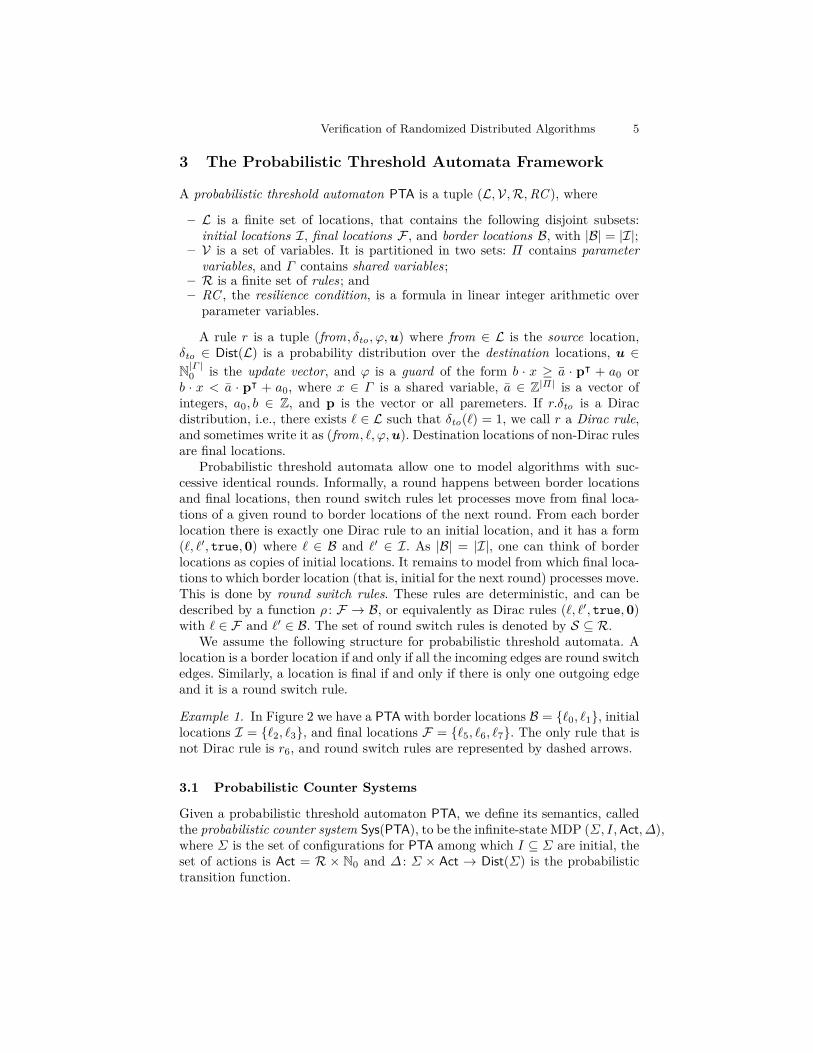
Given a PTA, we define a threshold automaton TAm such that for every non-Dirac rule r = (from, δto , ϕ,u) in PTA, all locations ` with δto(`) > 0 are mergedinto a new location `mrg in TAm. Note that this location must belong to F .Naturally, instead of a non-Dirac rule r we obtain a Dirac rule (from, `mrg, ϕ,u).Also we add self-loops at all final locations. The counter system Sysk(TAm) isdefined in the standard non-probabilistic way.

Figure 4 illustrates the transformation on our running example from Figure 2.The new final location `mrg represents a coin toss taking place; it belongs neitherto F0 nor F1.

`0

`1

`2

`3

`4`5

`mrg

r1

r2

r3 : x ≥ n− f 7→ y++

r4 : true 7→ x++

r5 : y ≥t

r7

r8

r9r6 : y < t

Fig. 4. A one-round non-probabilistic threshold automaton TAm obtained fromthe PTA from Figure 2.

Initial configurations in Sysk(PTArd) coincide with initial configurations inSysk(TAm). This exploits our definition of round-rigid adversaries, where all non-Dirac transitions are gathered at the end of a round.

Lemma 13. Fix k ∈ N0, an initial configuration σ from Sysk(PTArd), and around-rigid adversary s. For every LTL formula ϕ[k], the statements are equiv-alent:

(a) there exists π ∈ paths(σ, s) such that π |= ϕ[k] in Sysk(PTArd),(b) for every π ∈ paths(σ, s) holds π |= ϕ[k] in Sysk(TAm).

Proof. Paths in Sysk(TAm) are prefixes of paths in Sysk(PTArd). Moreover, sinceevery set of paths paths(σ, s) in Sysk(TAm) is a singleton, then existential anduniversal quantification coincide. ut

Finally, proving Probabilistic Wait-Free Termination under all round-rigidadversaries boils down to proving formula (16) on Sysk(TArd) and also thatSysk(TAm) |= A

∨v∈{0,1}G

∧`∈Fv

κ[`, k] = 0. Both can be checked by ByMC.Formally, from Corollary 1 and Lemma 13 we obtain the following.


Corollary 2. If Sysk(TArd) |= (16), and if

Sysk(TAm) |= A∨

v∈{0,1}

G∧`∈Fv

κ[`, k] = 0,

then Probabilistic Wait-Free Termination holds on Sys(PTA).

8 ExperimentsWe have applied the approach presented in Sections 4–7 to five randomizedfault-tolerant distributed algorithms 5:1. Protocol 1 for randomized consensus by Ben-Or [2]. We consider two kinds

of crashes: clean crashes (ben-or-cc) and dirty crashes (ben-or-dc). Duringa dirty crash a process can send to a subset of processes, while in cleancrashes a process is either sending to all proceses or none. This algorithmworks correctly when n > 2t.

2. Protocol 2 for randomized Byzantine consensus (ben-or-byz) by Ben-Or [2].This algorithm tolerates Byzantine faults when n > 5t.

3. Protocol 2 for randomized consensus (rabc-c) by Bracha [3]. It runs as ahigh-level algorithm together with a low-level broadcast that turns Byzantinefaults into “little more than fail-stop (faults)”. We check only the high-levelalgorithm for clean crashes. Our model checker produces counterexampleswhen Byzantine or Byzantine-symmetric faults are introduced in rabc-c. Themulti-layered protocol is designed for f < n/3 faults. However, our toolshows that rabc-c itself tolerates f < n/2 clean crashes.

4. k-set agreement for crash faults (kset) by Raynal [14], for k = 2. This algo-rithm works in presense of clean crashes when n > 3t.

5. Randomized Byzantine one-step consensus (rs-bosco) by Song and van Re-nesse [16]. This algorithm tolerates Byzantine faults when n > 3t, and itterminates fast when n > 7t or n > 5t and f = 0.

Following the reduction approach of Sections 4–7, for each benchmark, wehave encoded two versions of one-round threshold automata: an N-automatonthat models a coin toss by a non-deterministic choice, and a P-automatonthat never leaves the coin-toss location, once it entered this location. The N-automaton is used to support the non-probabilistic reasoning, while the P-automaton is used to prove probabilistic wait-free termination. Both automataare given as the input to Byzantine Model Checker (ByMC) [9], which imple-ments the parameterized model checking techniques for safety [6] and liveness [7]of counter systems of threshold-automata (for a bounded number of rounds andno randomization).

The automata follow the pattern shown in Figure 2: They start in one of theinitial locations (e.g., V0 or V1), progress by switching locations and incrementingshared variables and end up in a final location that corresponds to a decision(e.g., D0 or D1), an estimate of a decision (e.g., E0 or E1), or a coin toss (CT).5 The benchmarks and the instructions on running the experiments are available from:

https://forsyte.at/software/bymc/artifact82/

https://forsyte.at/software/bymc/artifact82/


Label Name Automaton FormulaS1 agreement 0 N A G (¬Ex{D0}) ∨ G (¬Ex{D1, E1})S2 validity 0 N A All{V0} → G (¬Ex{D1, E1})S3 completeness 0 N A All{V0} → G (¬Ex{D1, E1})S4 round-term N A fair → F All{D0, D1, E0, E1, CT}S5 decide-or-flip P A fair → F (All{D0, E0, CT} ∨All{D1, E1, CT})S1’ sim-agreement N A G (¬Ex{D0, E0} ∨ ¬Ex{D1, E1})S1” 2-agreement N A G (¬Ex{D0, E0} ∨ ¬Ex{D1, E1} ∨ ¬Ex{D2, E2})

Table 1. Temporal properties verified in our experiments for value 0 (the propertiesfor value 1 can be obtained by swapping 0 and 1). We write fairness constraints as fairto save space.

Table 1 summarizes the temporal properties that were verified in our exper-iments. Given the set of all possible locations L, a set Y = {`1, . . . , `m} ⊆ L oflocations, and the designated crashed location CR ∈ L, we use the shorthand no-tation: Ex{`1, . . . , `m} for

∨`∈Y κ[`] 6= 0 and All{`1, . . . , `m} for

∧`∈L\Y (κ[`] =

0∨ ` = CR). For rs-bosco and kset, instead of checking S1, we check S1’ and S1”.

Table 2. The experiments for rows 1-5 were run on a single computer (Apple MacBookPro 2018, 16GB). The experiments for row 6 (rs-bosco) were run in Grid5000 on 32nodes (2 CPUs Intel Xeon Gold 6130, 16 cores/CPU, 192GB). Wall times are given.

Automaton S1/S1’/S1” S2 S3 S4 S5# Name |L| |R| |S| Time |S| Time |S| Time |S| Time |S| Time1 ben-or-cc 10 27 9 1 5 0 5 0 5 0 5 02 ben-or-dc 10 32 9 1 5 1 5 0 5 0 5 13 ben-or-byz 9 18 3 1 2 0 2 0 2 0 2 14 rabc-cr 11 31 9 0 5 1 5 1 5 0 5 05 kset 13 58 65 3 65 17 65 12 65 39 65 406 rs-bosco 19 48 156M 3:21:00 156M 3:02:00 156M 3:21:00 n/a n/a 156M 3:43:12

Table 2 presents the computational results of our experiments. The meaningof the columns is as follows: column |L| shows the number of automata locations,column |R| shows the number of automata rules, column |S| shows the numberof enumerated schemas (which depends on the structure of the automaton andthe specification), column time show the computation times — either in secondsor in the format HH:MM:SS. For |R|, we give the figures for the N-automata, sincethey have more rules in addition to the rules in P-automata. To save space, weomit the figures for memory use from the table: Benchmarks 1–5 need 30–170MB RAM, whereas rs-bosco needs up to 1.5 GB RAM per cluster node.

The benchmark rs-bosco presents a challenge for the schema enumerationtechnique of [7]: Its threshold automaton contains 12 threshold guards that canchange their values almost in any order. Additional combinations are produced


by the temporal formulas. ByMC reduces the number of combinations by ana-lyzing dependencies between the guards. However, this benchmark requires us toenumerate between 11! and 14! schemas. To this end, we have run the verificationexperiments for rs-bosco on 1024 CPU cores of the computing cluster Grid5000.Table 2 presents the wall time results for rs-bosco, that is, the actual number ofcomputation hours on all the cores is the wall time multiplied by 1024.

For all the benchmarks in Table 2, ByMC has reported that the specificationshold. By varying the relations between the parameters (e.g., by changing n > 3tto n > 2t), we have found that rabc-cr can handle more faults, that is, t < n/2 incontrast to the original t < n/3 (the original was needed to implement the under-lying communication structure which we assume given in the experiments). Inother cases, whenever we changed the parameters, that is, increased the numberof faults beyond the known bound, the tool reported a counterexample.

9 Conclusions

In this paper we lifted the threshold automate framework to multi-round ran-domized algorithms. We proved a reduction that allows to check LTL-X speci-fications over propositions for one round in a single-round automaton so thatthe verifications results transfer directly to the infinite counter system. We haveshown, using round-based compositional reasoning, that this is sufficient to checkspecifications that span multiple rounds, e.g., agreement of consensus. We ap-plied a distinct reduction argument for almost sure termination under round-rigid adversaries.

By experimental evaluation we showed that the verification conditions thatcame out of our reduction can be automatically verified for several challengingrandomized consensus algorithms in the parameterized setting.

Our proof methodology for almost sure termination applies to round-rigidadversaries only. This restriction is crucial: transforming an adversary into around-rigid one while preserving the probabilistic properties over the inducedpaths, comes up against the fact that, depending on the issue of a coin tossin some step at round k, different rules may be triggered later for processesin rounds less than k. As future work we shall prove that verifying almost-sure termination under round-rigid adversaries is sufficient to prove it for moregeneral adversaries.

References

1. Baier, C., Katoen, J.P.: Principles of model checking. MIT Press (2008)2. Ben-Or, M.: Another advantage of free choice: Completely asynchronous agreement

protocols (extended abstract). In: PODC. pp. 27–30 (1983)3. Bracha, G.: Asynchronous byzantine agreement protocols. Inf. Comput. 75(2), 130–

143 (1987)4. Elrad, T., Francez, N.: Decomposition of distributed programs into communication-

closed layers. Sci. Comput. Program. 2(3), 155–173 (1982)


5. Fischer, M.J., Lynch, N.A., Paterson, M.S.: Impossibility of distributed consensuswith one faulty process. J. ACM 32(2), 374–382 (1985)

6. Konnov, I., Lazic, M., Veith, H., Widder, J.: Para2: Parameterized path reduc-tion, acceleration, and SMT for reachability in threshold-guarded distributed al-gorithms. Formal Methods in System Design 51(2), 270–307 (2017)

7. Konnov, I., Lazic, M., Veith, H., Widder, J.: A short counterexample property forsafety and liveness verification of fault-tolerant distributed algorithms. In: POPL.pp. 719–734 (2017)

8. Konnov, I., Veith, H., Widder, J.: On the completeness of bounded model checkingfor threshold-based distributed algorithms: Reachability. Information and Compu-tation 252, 95–109 (2017)

9. Konnov, I., Widder, J.: Bymc: Byzantine model checker. In: ISoLA (3). LNCS, vol.11246, pp. 327–342. Springer (2018)

10. Kwiatkowska, M.Z., Norman, G.: Verifying randomized byzantine agreement. In:FORTE. pp. 194–209 (2002)

11. Kwiatkowska, M.Z., Norman, G., Parker, D.: PRISM 4.0: Verification of proba-bilistic real-time systems. In: CAV. pp. 585–591 (2011)

12. Kwiatkowska, M.Z., Norman, G., Segala, R.: Automated verification of a random-ized distributed consensus protocol using cadence SMV and PRISM. In: CAV. pp.194–206 (2001)

13. Lehmann, D.J., Rabin, M.O.: On the advantages of free choice: A symmetric andfully distributed solution to the dining philosophers problem. In: POPL. pp. 133–138 (1981)

14. Mostefaoui, A., Moumen, H., Raynal, M.: Randomized k-set agreement in crash-prone and byzantine asynchronous systems. Theor. Comput. Sci. 709, 80–97 (2018)

15. Nestmann, U., Fuzzati, R., Merro, M.: Modeling consensus in a process calculus.In: CONCUR. pp. 393–407 (2003)

16. Song, Y.J., van Renesse, R.: Bosco: One-step Byzantine asynchronous consensus.In: DISC. LNCS, vol. 5218, pp. 438–450 (2008)


APPENDIX

A Detailed Definition of the Underlying Counter Systems

Definition 7. Given a probabilistic counter system Sys(PTA) = (Σ, I,Act, ∆),we define its non-probabilistic version Sysnp(PTA) to be the tuple (Σ, I,R),where R is a transition relation defined below.

If Act = R × N0 and if Rnp is defined from R as in Definition 2, thentransitions are tuples t = (r`, k) ∈ Rnp × N0 such that α = (r, k) is an actionfrom Act and for ` ∈ L holds that α.δto(`) > 0. Transition t is unlocked in aconfiguration σ from Sysnp(PTA) if α is unlocked in σ in Sys(PTA). Similarlywe define when t is applicable to σ. We obtain σ′ by applying an applicabletransition t to σ, written t(σ) = σ′, if and only if there exists a location ` ∈ Lsuch that apply(α, `, σ) = σ′.

Two configurations σ and σ′ are in the transition relation R, i.e., (σ.σ′) ∈ R,if and only if there exists a transition t such that σ′ = t(σ).

Definition 8. Given an arbitrary TA = (L,V,Rnp ,RC ), with border, initial,and final location sets B, I, and F , respectively, we define its infinite countersystem Sys∞(TA) to be the tuple (Σ, I,R). Configurations from Σ and I aredefined as in Section 3.1. A transition t is a tuple (r`, k) ∈ Rnp × N0. Since itcoincides with Dirac actions, we define when a transition is unlocked in a configu-ration and when it is applicable to a configuration, in the same way as for a Diracaction in Section 3.1. A configuration σ′ is obtained by applying an applicabletransition t = (r`, k) to σ, written σ′ = t(σ), if and only if apply(α, `, σ) = σ′,for a Dirac action α = (r`, k) and the destination location ` of r.

Now we have (σ, σ′) ∈ R, if and only if there exists a transition t such thatσ′ = t(σ).

PTA TA

Sys∞(TA)

Sys(PTA) Sysnp(PTA)

Definition 2

Section 3.1

Definition 8

Definition 7

=

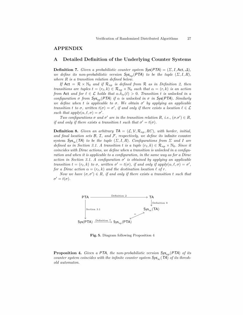
Fig. 5. Diagram following Proposition 4

Proposition 4. Given a PTA, the non-probabilistic version Sysnp(PTA) of itscounter system coincides with the infinite counter system Sys∞(TA) of its thresh-old automaton.


It is easy to see that the diagram from Figure 5 commutes, and thus ev-ery PTA yields the unique non-probabilistic counter system. The two construc-tions give us possibility to remove probabilistic reasoning either on the level ofa PTA (using Definition 2) or on the level of a counter system Sys(PTA) (usingDefinition 7). Therefore, for different reasoning we will refer to the constructionthat is more convenient.

verification of randomized distributed algorithms under

Documents