Proceedings of CHT-04ICHMT International Symposium on Advances in Computational Heat Transfer

April 19-24, 2004, Norway

CHT-04-179

VERIFICATION AND VALIDATION OF EFD.Lab CODEFOR PREDICTING HEAT AND FLUID FLOW

V. Balakin*°, A. Churbanov*,**, V. Gavriliouk*, M. Makarov *and A. Pavlov*

*NIKA Software, 4 Volokolamskoye Shosse, 125993 Moscow, Russia**Institute for Mathematical Modeling, 4-A Miusskaya Sq., 125047 Moscow, Russia°Correspondence author: Fax: +7 (095) 785-5748 Email: balakin@nika.sokol.ru

ABSTRACT Results of verification and validation of commercial code EFD.Lab are presented in thispaper. Two classes of tests – so-called fundamental as well as applied industrial – are considered forheat and fluid flow phenomena. A flow over a circular cylinder with internal heating and buoyancy-driven flow in a square cavity have been predicted among fundamental tests in a wide range ofgoverning parameters. Another examples that demonstrate accuracy and efficiency of EFD.Lab tosolve applied problems of practical interest are concerned with electronic cooling. Pin-fin and plainconfigurations of heat sinks have been predicted in the free and forced convection regimes,respectively, taking into account radiation effects. Grid convergence studies have been performedduring validation predictions. A good agreement has been obtained between numerical andexperimental data in all predicted tests in a wide range of computational grids.

INTRODUCTION

This work is concerned with verification and validation (V&V) of the commercial code – EFD.Lab(Engineering Fluid Dynamics Laboratory), a product of NIKA GmbH (www.nika.biz) - a general-purpose CFD code that belongs to a new generation of codes based on recent achievements in user-friendly interface as well as highly accurate, robust and automatic numerics.

The basic concept put into the background of designing EFD.Lab is to maximize as high as possibleautomatization level in preparing, performing and visualizing predictions of real appliedengineering problems. This tendency to make CFD tools less expensive as well as easier and closerto engineers only recently has been "discovered" and taken to implementation in The Big Three ofCFD - Fluent, CFX (recently purchased by ANSYS Inc.), and STAR-CD (CD adapco Group) [1].

In comparison with traditional CFD codes oriented to high-level specialists in CFD (Ph.D. as therule), EFD.Lab is designed for a wider category of users – engineers of different special interest. Intheir daily activities they occasionally face the necessity to solve complex industrial problemscoupled with heat and fluid flow phenomena. To accomplish these ends, EFD.Lab has somespecific features, namely: complete integration with CAD-systems; totally automatic gridgeneration; automatic prescribing of computation control parameters; user-friendly pre- and post-processing; a possibility to perform a parametrical study of a problem etc. The code does notrequire tuning a somewhat mystique parameters of the algorithm or choosing one of several notvery clear models or approximations. These combined possibilities allow accelerating essentially

solution of day duty problems for an engineer but imposing high requirements on accuracy andreliability of such an automatic approach. That is why during its development EFD.Lab has beenexposed to the detailed verification and validation (V&V) procedure on a host of analytical andbenchmark solutions as well as on experimental results available from publications and databases[2,3]. Some of the results are discussed in the present work with particular emphasis on the heattransfer phenomenon.

EFD.Lab: MODELS, MESHES, NUMERICS AND LINEAR SOLVER

Below there are briefly listed features of EFD.Lab.

Models The employed in the code numerical method is designed for laminar and turbulent flowsranging from incompressible to highly compressible flows. Heat transfer simulation includesforced, natural and mixed convection, conjugate heat transfer in solids and liquids, radiation etc.

The approach is based on the Reynolds-Averaged Navier-Stokes equations. The energyconservation equation for the total enthalpy in a fluid and temperature in a solid media along with aspecially designed model of energy exchange on a solid-liquid interface are used to govern heattransfer.

Sub-grid flow field peculiarities such as vortices and boundary layers are resolved using thefollowing integral techniques: modified (k-ε )-turbulence model describing laminar, mixedlaminar/turbulent and turbulent regimes coupled with an original near-wall laminar/turbulentmodel.

Meshes The code essentially exploits adaptive mesh refinement strategy [4,5] that provides anautomatic adaptation of a Cartesian computational grid to the complicated geometry of acomputational domain (static adaptation) and to the solution peculiarities (dynamic adaptation).This allows combining merits of employing high order spatial approximations and local resolutionof solution or geometry singularities without essentially increasing the number of cells. Grid cellsare treated as control volumes and can belong completely to a fluid or solid, or contain both media.In the last case two phases are separated by a surface where heat and fluid flow should beconsidered in a specific way.

Numerics The finite volume method is utilized to derive conservative discrete equations [6-9]. Allcalculated unknowns are referred to cell mass centers, i.e. the collocated grid is used. Themomentum components, pressure and total enthalpy are considered as the primary variables.

An operator-splitting technique similar to SIMPLE-type methods (so-called pressure-correctionmethods) in the time-dependent formulation is used to resolve the pressure-velocity coupling.Following the approach, firstly, the continuity and momentum equations are discretized, and thenthe discrete pressure correction equation is derived by means of algebraic transformations of theoriginal grid equations with incorporated boundary conditions for momentum [10]. Usage ofspecially designed consistent approximations for operators of divergence in the continuity equationand gradient in the momentum equation leads to a linear system with the matrix that is close tosymmetric positive definite one.

Second order approximations are used for all spatial operators, including convective terms. Toprovide monotonic solutions, non-linear flux approximations with limiters (like in the TVDapproach) are employed for convective terms. Considering heat transfer problems, a singlealgebraic system is derived for solid and fluid media (the conjugate formulation of a thermalproblem).

Multigrid solver Grid equations arising from discretization and linearization of the governingPDEs are solved using multigrid technique [11,12], thus obtaining near linear performance in termsof computational effort, as the mesh finesse increases.

Building the series of coarse meshes and appropriate linear system matrices is fully automatic andindependent of the way the computational mesh is constructed. The Galerkin operators are used onthe coarse grids. This ensures high (fine mesh cell number)/(coarse mesh cell number) ratio. Nodiscretization on the sequence of coarse meshes is needed.

Automatic coarse grid construction takes full advantage of structured locally refined rectangularhexahedral mesh. To speed up the coarse grid construction, binary tree-like ordering of mesh cellsis introduced. This facilitates addressing mother cell and neighbor cells in the construction process.Once a coarse mesh is built, block technique is used, that allows associating a pack of unknownswith any cell of any mesh (background computational or any coarse one). This feature improvesperformance in cases with complex geometry of computational domain. Since the domain geometrycannot be resolved on coarse grids, treads of unknowns are automatically tracked through thecoarsening process, so that the pack in any cell is formed by representatives of different treads.Treads vanish as their representatives become involved in linear equations on coarse grids withother tread representatives.

The same technique is exploited when more than one unknown of the original linear system isassociated with a cell of the mesh. Solving for temperature in the conjugated heat transfer modelcan be an example. On a subset of mesh cells, both fluid temperature and solid body temperatureare components of the coupled system that is solved using multigrid technique sharing the same setof coarse grids.

As smoothers, Gauss-Seidel type relaxation methods are used, which are enhanced, if necessary, byintroducing point-wise local iterative parameter. The choice of the parameter is sensitive to thegenuine differential equation and the way it is approximated.

VERIFICATION AND VALIDATION METHODOLOGY

There do exist a good many approaches to V&V-procedure analyzed, e.g., in [13-15]. In ourpractice we employ for V&V procedure the benchmark results that, in our mind, can bedecomposed into two classes – the so-called fundamental tests and applied industrial ones. Each ofthese classes has its own merits and demerits, but these two types complement each other nicelyand are used successfully for the V&V-procedure of EFD.Lab. Let us consider these two classes forthermal problems.

The first class is the fundamental tests which are simple enough in sense of geometry (2D as therule) and problem formulation (reduced models, exact boundary conditions etc.). On these low costtests it is possible to conduct a parametrical study of various regimes of heat and fluid flow in amaximally wide range investigated experimentally, numerically or analytically. Moreover,versatility of fundamental tests allows investigate practically on the same configuration variousphysical effects in coupled or decoupled manner or even in artificial formulation in order tohighlight their specific impact.

The second one – applied industrial problems where in addition to the complicated 3D geometry acombination of different strongly coupled physical phenomena takes place. Moreover, the exactvalues of material properties as well as operating conditions for device components are necessary inthis case and so, the level of uncertainty is here much higher.

The automatic settings of the code input parameters are used in V&V-procedure calculations: thetotally automatic grid generation, settings for control and calculation parameters as well as forstopping criteria are taken by default and so on. It is also possible to construct grids in a non-automatic way – uniform or stretching grids in accordance with input parameters specified by auser. Such simple grids are used for predictions or convergence studies inrectangular/parallelepiped computational domains.

The grid convergence is studied thoroughly for all tests: a series of calculations is carried out atdifferent Result Resolution Level (RRL) – an input parameter for the code ranging from 1 up to 8and increasing grid adaptation (and as the consequence its size) as well as convergence criteria. Infact, it is an integral parameter prescribing accuracy of predictions. The value of RRL that indicatesno essential variation in computational results at its further increasing is treated as the final one andis recommended for a user.

FUNDAMENTAL TESTS

Flow over a circular cylinder with heating A flow over a circular cylinder is a remarkable test dueto a host of data available for a comparison [16-19] where results of many researches areaccumulated. Very useful guide [18,19] should be highlighted because there are condensed practicallyall experimental and numerical results derived for many years. Even in the 2D formulation this problemallows to investigate various regimes - steady-state and periodically oscillating, laminar and turbulent,and moreover, to study influence of such physical effects as compressibility, heat transfer, surfaceroughness, cylinder oscillation, cavitation, rheology (non-newtonian fluids) etc.

The simplest modification of this problem in order to involve heat transfer phenomenon is toconsider a cylinder heated by the uniformly distributed in it a volumetric heat source with the totalheat generation rate q [20]. Convective heat transfer from a heated circular cylinder in an air flowwas studied numerically via EFD.Lab at Reynolds number ReD from 1 up to 105, i.e. there wereinvestigated flow regimes from steady-state up to developed transient flows with separation oflaminar or turbulent boundary layer and as the consequence, various conditions of heat transferwere under the consideration.

The results of the grid convergence study for this problem are presented in Fig. 1 for Re = 104 as thedependence of predicted Nusselt number NuD on the value of RRL parameter. Here NuD = h D/k (his the heat transfer coefficient averaged over the cylinder, and k - fluid thermal conductivity), andthe Prandtl number Pr = 0.72 for all values of ReD. Evidently, EFD.Lab predictions lie withinbounds of experimental data which have a large dispersion in this turbulent flow regime.

0.00E+00

2.00E+01

4.00E+01

6.00E+01

8.00E+01

0 1 2 3 4 5 6 7 8 9

RRL value

Nu

Calc. Exp. Max Exp. Min

Figure 1. Grid convergence study: Nusselt number NuD vs. RRL valuein comparison with experimental data from [20], Re = 104.

A good correlation in NuD between transient computations and measurements [20] has beenobtained in the whole considered range of ReD (see Fig. 2).

0.1

1

10

100

1000

0.1 1 10 100 1000 10000 100000 1000000

Figure 2. Nusselt number NuD for air flow over a heated cylinder: EFD.Lab predictions (red dots)in comparison with experimental data from [20] (black circles).

Buoyancy-driven cavity flow The well-known problem of a buoyancy-driven flow in a squarecavity [21] has been considered, too. This 2D test is classical for convective heat transfer andallows to evaluate calculations quality in a simple geometry for the Rayleigh number varying from103 up to 106. The benchmark solution [21] has been obtained from high-accurate predictions ofabout 40 computer codes and moreover, it agrees very well with the semi-empirical formula ofexperimental researches [22]. Nowadays this problem becomes a popular 3D test for variouscommercial and in-house codes [23]. In this 2D test a free convection is considered in a squarecavity with isothermal side walls of different temperature value and the thermally insulated top andbottom. Air with variable properties has been used in EFD.Lab predictions of this problem.

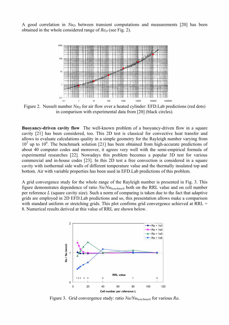
A grid convergence study for the whole range of the Rayleigh number is presented in Fig. 3. Thisfigure demonstrates dependence of ratio Nu/Nubenchmark both on the RRL value and on cell numberper reference L (square cavity size). Such a norm of comparing is taken due to the fact that adaptivegrids are employed in 2D EFD.Lab predictions and so, this presentation allows make a comparisonwith standard uniform or stretching grids. This plot confirms grid convergence achieved at RRL =8. Numerical results derived at this value of RRL are shown below.

0

1

2

0 20 40 60 80 100 120

Cell number per reference L

Nu /

Nu b

ench

Ra = 1e3Ra = 1e4Ra = 1e5Ra = 1e6

1 2 3 4 5 6 7 8RRL value

Figure 3. Grid convergence study: ratio Nu/Nubenchmark for various Ra.

Figure 4 shows the particular case of Ra = 106, predicted at the highest RRL = 8. The mesh derivedin this prediction after the dynamic adaptation to the solution peculiarities is shown in Fig. 5. It iseasy to see that this mesh matches well the features of heat and fluid flow.

Figure 4. Temperature and velocity fields, predicted at RRL = 8 for Ra = 106.

Figure 5. Adapted to the solution mesh at RRL = 8 for Ra = 106.

The next figures demonstrate a good agreement between EFD.Lab predictions and the benchmarksolution both in thermal (see Fig. 6 for the average Nusselt number) and hydrodynamic (see Fig. 7for the maximum velocity components) fields for all considered values of the Rayleigh number.

01

23

45

67

89

10

1.00E+03 1.00E+04 1.00E+05 1.00E+06

Ra

Nu a

v

Nu av benchNu av calc

Figure 6. Predicted average Nusselt number vs. Rayleigh numberin comparison with the benchmark solution [21].

1

10

100

1000

1.00E+03 1.00E+04 1.00E+05 1.00E+06

Ra

U, V

U max benchV max benchU max calcV max calc

Figure 7. Predicted maximum velocity components vs. Rayleigh numberin comparison with the benchmark solution [21].

In the above fundamental tests the V&V procedure were performed separately for various physicaleffects. Application of EFD.Lab to applied industrial problems with different strongly coupledphysical phenomena is presented in the next section.

APPLIED INDUSTRIAL PROBLEMS

The next examples that demonstrate possibility of EFD.Lab to solve problems of practical interestwith appropriate accuracy are concerned with electronic cooling.

Nowadays with the increasing of heat dissipation from electronic devices and the reduction of theirsizes, thermal management becomes more and more essential element of electronic product design[24]. To increase life and reliability of electronic equipment, it is necessary to preserve itscomponent temperatures within the limits specified by the device design engineers. Heat sinks ofvarious types are the devices constructed to resolve this problem - they enhance heat dissipationfrom a heat-generating component to air. To optimize performance of a particular heat sink, up-to-date CFD tools are in common use.

Code EFD.Lab demonstrates a very high efficiency and automatic in solving problems of such type.Below there are presented two examples of using EFD.Lab to predict the performance heat sinks atvarious operating conditions for V&V procedure.

Free convection cooling Performance of a pin-fin heat sink at free convection cooling of air hasbeen studied in [25] both experimentally and numerically using an in-house code. The case of 9x9square pin-fin array from this work has been investigated via EFD.Lab and compared withmeasurements.

Our model used in computations (see Fig. 8) totally reproduces the experimental configuration from[25] presented in Fig. 9 in detail. It consists of two rectangular plexiglass enclosures put one insideanother. The internal enclosure with aluminium pin-fin array over the heating component flushmounted on the bottom (see Fig. 10) is of actual interest. The external one was employed inexperiments only to create natural convection environment. Nevertheless, a half of the whole two-enclosure model (the green domain in Fig. 8) has been used in our predictions in order to reproduceexactly the actual experiments (in contrast to [25] where only the internal enclosure has beenconsidered in calculations).

Figure 8. The two-enclosure model with a small box in the wall at the uppercorner of the external enclosure for monitoring Tamb.

Figure 9. Geometry of enclosures with pin-fin arrays on heating component (from [25]).

Figure 10. A part of the model: the internal enclosure with 9x9 pin-fin arrayover the heating component flush mounted on the bottom.

Performance of the pin-fin heat sink has been studied experimentally in [25] at various heatgeneration rate - q = 0.1, 0.3, 0.5, 0.7 and 1 W – for two configurations of the device – thehorizontal case (the gravity force is along y-axis) and the vertical one (the gravity force acts alongx-axis of the model).

As it was mentioned above, only the heat sink and heating component are made of aluminium(thermal conductivity k = 200 W/mK), other elements (all walls except for the bottom of theexternal enclosure) are of plexiglass with k = 0.2 W/mK. The conjugate formulation of the thermalproblem in addition to convection and conduction phenomena also includes radiation effects thatare essential in this problem (about 50% as it was estimated in [25]). The surface emissivity of the

black painted internal enclosure bottom and pin-fin array was ε = 0.95 and the remaining surfacesof both enclosures are 0.83. The bottom of the external enclosure was made of insulator.

It should be noted that this problem does have some features that make it complicated enough forcalculations. First, it has various scales of the model elements: the length of the external enclosure Lis 0.635 m, the thickness of the heating component is δ = 0.000861 m and pin fins are of0.0015х0.0015 m cross-section, i.e. ratio L/δ = 737.5 is very high. It should be mentioned that incomputations [25] a porous media model has been used to describe the heat sink in order to simplifyessentially the problem geometry. Secondly, heat transfer includes conduction, convection andradiation effects and involves materials with different thermal properties. Next, heat generation rateq is very small – in the range from 0.1 up to 1 W – with the primary searching parameter Rt=(Tj-Tamb)/q. For q = 0.1 W the searching temperature drop in Rt is about 5.6 °С that means that foragreement of predictions with measurements within 5 % the temperature field should be predictedwith accuracy 0.3 °С. Temperature measurement uncertainty in [25] was estimated as ±0.1 °С thatcompletely satisfies these requirements.

The basic parameter for heat sink efficiency is the thermal resistance between a very thin heatingcomponent with prescribed heat generation rate q located under the heat sink and ambient air flow –Rt=(Tj-Tamb)/q – where Tj is the maximum temperature of the heating component. Namely thisparameter was the primary goal of steady-state predictions. As it was mentioned above, a small boxin the wall at the upper corner of the external enclosure was employed in EFD.Lab predictions formonitoring Tamb.

In spite of the fact that experiments [25] were well-designed in order to minimize the environmentimpact, inhomogeneous temperature distributions can appear on the outer surfaces of the externalenclosure walls due to radiation and convection. To study these effects, three kinds of boundaryconditions (except for the insulator) have been considered in EFD.Lab predictions:

- the Newton law of ambient air cooling with convection heat-transfer coefficient h estimatedfollowing [20] for the wind-free case. This coefficient depends on the heat generation rate ofthe component as well as surface position (vertical or horizontal). The values of h were 0.6and 1.9 W/m2 K for side walls and the top, respectively, in the case of q = 0.1 W. For valuesof heat generation rate q = 0.3-0.7 W values of h were, respectively, 0.73 and 2.3 W/m2 K,and for q = 1 W these are 0.9 and 3 W/m2 K. A small box in the wall at the upper corner ofthe external enclosure was employed in EFD.Lab predictions for monitoring Tamb (seeFig. 8).

- Isothermal outer wall with specified temperature Tw = 20 °С (it is a standard enough valuefor environment).

- Uniform surface heat sinks of equivalent total rate –q are imposed. This type of theboundary conditions requires no experimental parameters but assumes some distribution ofsurface sinks (which, in general, may be non-uniform and can be evaluated from preliminarypredictions with other boundary conditions).

The initial temperature was Tini = 20 °С in all predictions. No-slip, no-permeability conditions forfluid flows were imposed on all internal solid walls.

The whole range of heat generation rate q has been investigated numerically for both configurationsof the device. The obtained numerical results are very close to experimental data [25] both forthermal and hydrodynamics parameters and indicate for Rt agreement with measurements within5% for all considered cases.

Let us consider now the grid convergence study. EFD.Lab essentially exploits adaptive meshrefinement strategy where we have the basic mesh corresponding to the coarser level and successivemesh refinement near boundaries and/or specified objects. The finest grid used in computations has

the basic mesh of 82х52х38 with the total number of cells as high as 375,896 cells (see Figs. 11 (a)and (b), showing various fragments of this mesh along with temperature contours predicted for q =1 W).

(a) Temperature contoursand mesh in sections

(b) Temperature contoursand mesh on heat sink

Figure 11. Temperature contours and fragments of the mesh on various surfaces.

So, three grids have been considered for a half of the model with basic meshes of various size withstretching to the external enclosure - 28х18х14 (26,194 cells totally)), 56х35х28 (145,082 cellstotally) and 82х52х38 (375,896 cells totally).

Calculations with various boundary conditions have indicated that two types of them - the specifiedheat-transfer coefficient and imposed uniform surface heat sinks of equivalent total rate –q –provide practically the same numerical results. Predictions with prescribed boundary temperatureTw = 20 °С give the worst results in sense of agreement with experimental Rt . Therefore, allnumerical results presented here correspond to the Newton law of ambient air cooling as the mostuniversal for engineering applications type of boundary conditions.

The grid dependence of numerical results on the mesh size is shown in Fig. 12 for two values of q –the minimal and maximal ones - for the vertical configuration of the device. Figure 13 demonstratesa comparison of predicted and measured thermal resistance Rt for different q derived on the finestgrid with 375,896 cells. It should be noted again that for all values of q the numerical results arewithin 5% from experimental data – an excellent correlation between computations andmeasurements.

30

40

50

60

70

0 100000 200000 300000 400000

Number of cells

Rt (K

/W)

Cal. Q = 0.1 W Exp. Q = 0.1 WCal. Q = 1 W Exp. Q = 1 W

Figure 12. Grid convergence: predicted Rt vs. total cells number,q = 0.1 and 1 W, vertical case.

30

35

40

45

50

55

60

0 0.5 1

Q (W)

Rt (K

/W)

ExperimentsPredictions

Figure 13. Comparison of predicted and measured thermal resistance Rtfor different q, vertical case.

Figure 14 demonstrates flow trajectories colored by the velocity magnitude in both enclosures forthe case of q = 1 W. It is easy to see that the flow is fully 3D and so, it is difficult enough toconstruct computational flow patterns for comparing with the experimental visualization.

Figure 14. Flow trajectories colored by the velocity magnitude in both enclosures, q = 1 W.

Figure 15 shows a comparison of visualization from [25] with predicted flow pattern for q = 1 Wderived on the finest grid. Obviously, a very good agreement is observed here.

(a) Velocity vectors (b) Flow trajectories (c) Vizualization [25]

Figure 15. Predicted velocity vectors (a) and flow trajectories colored by velocity magnitude (b)in compare with vizualization from [25] (c), q = 1 W, z = 0 m.

A very good coincidence of numerical and experimental results has been obtained for the horizontalconfiguration of the device, too.

The next figures present a detailed comparison of the predicted flow pattern (see Figs. 16 and 17)with experimental vizualization from [25] (see Fig. 18) for the intermediate value of the heatgeneration rate q = 0.5 W.

Figure 16. Predicted velocity vectors in the internal enclosure, q = 0.5 W, z = 0 m.

Figure 17. Predicted flow trajectories colored by velocity magnitude, q = 0.5 W.

Figure 18. Visualization from [25], q = 0.5 W, z = 0 m.

Increasing of the heat generation rate results in a more intensive flow in both enclosures (seeFig. 19).

Figure 19. Flow trajectories in both enclosures, q = 1 W.

For this case with q = 1 W a good agreement is also observed between numerical and experimentalresults presented in Figs. 20, 21 and 22, respectively.

Figure 20. Predicted velocity vectors in the internal enclosure, q = 1 W, z = 0 m.

Figure 21. Predicted flow trajectories colored by velocity magnitude, q = 1 W.

Figure 22. Visualization from [25], q = 1 W, z = 0 m.

Forced convection cooling Another type of heat sinks – plane ones – has been also studiednumerically using EFD.Lab. Wind tunnel experimental results from [26] have been used forvalidation and verification of EFD.Lab predictions of forced air cooling in a duct. The mostcomplicated case with the dense heat sink (32 plates) and large clearance (30% in all directions) hasbeen considered.

The duct of rectangular cross-section has a heating component flush mounted on the bottom withplain heat sink of 32 plates located over it (see Fig. 23). Internal sizes of the duct are L = 0.61 m, W= 0.0923 m and H = 0.0663 m. All its walls are made of FR-4 (fiberglass-epoxy laminate boardwith thermal conductivity k = 0.35 W/mK) with thickness δ = 0.005 m. A fan provides a uniformvelocity profile of air with Tamb = 25 °С at the duct inlet. The opening with the atmospheric pressureis at the duct outlet. The heating component (k = 220 W/mK) with L = 0.11 m, W = 0.071 m and H

= 0.0005 m is located at the distance of 0.17 m from the inlet with the heat generation rate 100 W.To enhance heat transfer from it, the heat sink is attached to the top. It consists of the aluminiumbase (k = 220 W/mK) with height H = 0.005 m and 32 plates (k = 150 W/mK) with H = 0.045 mand W = 0.0005 m located in a duct in the side-inlet-side-exit (SISE) configuration with respect toan incoming air flow (see Fig. 24).

Figure 23. The computational model.

Figure 24. SISE-configuration of plain heat sinks (from [26]).

Steady-state heat and fluid flows have been calculated in a half of the model for two values of theinlet velocity u, namely, 3 and 5 m/s. Radiation between the heat sink (emissivity ε = 0.9) and ductwalls (ε = 0.9) was taken into account in addition to convection and conduction. At the outersurfaces of all walls (except for the thermally-insulated bottom) there is imposed the Newton law ofambient air cooling with convection heat-transfer coefficient h = 5.6 + 4*u (W/m2 K), taken from[27] for the wind case, where u is the inlet velocity, supplemented with radiation into the non-radiative environment.

In addition to measurements some numerical results obtained via code IcePak developed byFLUENT Inc. are presented in work [26]. It is not clarified clearly in this work are radiation effectsessential or not in this problem at the considered regimes. Estimated Reynolds numbers are lowenough for the considered flow regimes. Predictions via code IcePak have been conducted in tworegimes – laminar and turbulent – and indicated different agreement with measurements, namely,7% error in laminar and 15-20% error in turbulent predictions, respectively (grid was between110,000 and 210,000 elements). EFD.Lab predictions have been carried out in the laminar regimebecause local Reynolds number for the flow between plates is lower 500 for all inlet velocities.Calculations have indicated that omitting radiation results in overprediction of the thermalresistance on about 10%. Only taking into account the radiative fluxes from all surfaces it ispossible to obtain numerical results maximally close to measurements.

For the grid convergence study three grids have been considered for a half of the model with basicmeshes of various size - 30х11х17 (90,107 cells totally), 45х16х22 (203,972 cells totally) and68х24х24 (456,872 cells totally). The grid convergence of the solution for u = 3 and 5 m/s ispresented in Fig. 25. Figure 26 demonstrates a comparison of predicted and measured thermalresistance Rt for different u obtained on the finest grid with 456,872 cells. Agreement betweennumerical results and measurement data was within 5% for both velocity values - a very good resultagain.

0.10.120.140.160.180.2

0 200000 400000 600000

Number of cells

Rt (K

/W)

Cal. V = 3 m/s Exp. V = 3 m/sCal. V = 5 m/s Exp. V = 5 m/s

Figure 25. Grid convergence: predicted Rt vs. total cells number for u = 3 and 5 m/s.

0.1

0.12

0.14

0.16

0.18

0.2

2 3 4 5 6

V (m/s)

Rt (K

/W)

PredictionsExperiments

Figure 26. Comparison of predicted and measured thermal resistance Rt for different u.

Predicted flow trajectories and the temperature field are shown for u = 5 m/s in Figs. 27 and 28,respectively. Contours of the temperature and velocity module in transverse cross-section x = 0.25m are presented in Fig. 29.

Figure 27. Flow trajectories (colored by velocity magnitude) in the duct, u = 5 m/s.

Figure 28. Temperature contours in the vicinity of plane sink, u = 5 m/s, z = 0 m.

(a) Temperature (b) Velocity moduleFigure 29. Contours of the temperature (a) and velocity module (b), u = 5 m/s, x = 0.25 m.

Figure 30 demonstrates contours of the temperature and the adaptive computational grid with456,872 cells in longitudinal (z = 0 m) and transverse (x = 0.225 m) cross-sections, respectively.

Figure 30. Contours of the temperature and the adaptive gridin cross-sections z = 0 m and x = 0.225 m, u = 5 m/s.

To show efficiency of the solver, the total computation time divided by the total number of cellsand by the number of iterations is depicted in Fig. 31 for both above problems. These datacorrespond the vertical configuration with q = 1 W for the pin-fin sink and u = 5 m/s for the planeheat sink. It should be noted that the number of iterations was the same for all computational gridsand equaled 400 for the pin-fin sink problem and 150 for the forced convection cooling. Evidently,the solver used for solving grid equations at each iteration, indicates the number of arithmeticoperations proportional to the number of grid points (cells). All runs have been performed using PCwith a processor of 2.8 Ghz. Runs on appropriate in sense of accuracy grids required about 4 hourson the grid with 145,082 cells for the pin-fin sink problem and about 2.7 hours on the grid with203,972 cells for the plane heat sink – it is a good result for such a class of heat and fluid flowproblems.

00.0001

0.0002

0.0003

0.0004

0.0005

0 200000 400000 600000

Number of cells

CPU

/ Nce

lls /

Nite

r

Pin-Fin Sink Plane Sink

Figure 31. CPU time per cell per iteration vs. number of cells.

CONCLUSION

As the rule, practically any attempt to reproduce experimental results for an applied industrialproblem faces the necessity to reconstruct absent input data via human imagination. This isespecially true with respect to thermal problems because heat transfer phenomenon is coupled withvarious effects (radiation, variation in material properties etc.) and their impact on experimentaland/or numerical results is unknown a priori. So, experiments with complete and sufficientlyaccurate data for all input parameters are necessary. Measurements from [25] are a good example ofsuch a well-designed experimental work.

A very good agreement has been obtained between numerical and experimental data in all presentedhere examples of EFD.Lab predictions. Needless to say that this collection should be and will bemore and more wide. But even now it is obvious that EFD.Lab can serve as an efficient tool tostudy engineering problems including the heat transfer phenomenon.

Notwithstanding a lot of databases with complicated CFD tests, fundamental tests continue toprovide an essential part of the V&V-procedure due to their low cost in time and the possibility tostudy on a single model a wide range of heat and flow regimes and effects.

REFERENCES

1. Elliot, L., CFD Applications Soar: Part Two, CFD Review, June 11, 2003(http://www.cfdreview.com/articles/).

2. Freitas, C.J., Perspective: Selected Benchmarks From Commercial CFD Codes, Trans. ASME, J.Fluids Engrg., Vol. 117, No. 2, pp 208-218, 1995.

3. Fluid Dynamics Databases, ERCOFTAC Bulletin, No. 52, 2002.

4. Berger, M.J. and Oliger, J., Adaptive Mesh Refinement for Hyperbolic Partial DifferentialEquations, J. Comput. Phys., Vol. 53, No. 3, pp 482-512, 1984.

5. Berger, M.J. and Colella, P., Local Adaptive Mesh Refinement for Shock Hydrodynamics, J.Comput. Phys., Vol. 82, No. 1, pp 64-84, 1989.

6. Gavrilyuk, V.N., Denisov, O.P, Nakonechny, V.P., Odintsov, E.V., Sergienko, A.A. andSobachkin, A.A., Numerical Simulation of Working Processes in Rocket Engine CombustionChamber, 44th Congress of the Int. Astronautical Federation, Graz, Austria, October 16-22,1993, IAF-93-S.2.463, pp 1-15.

7. Krulle, G., Gavriliouk, V., Schley, C.-A. and Sobachkin, A., Numerical Simulation Technologyof Aerodynamic Processes and Its Applications in Rocket Engine Problems, 45th Congress ofthe Int. Astronautical Federation, Jerusalem, Israel, October 9-14, 1994, IAF-94-S2.414, pp 1-12.

8. Hagemann, G., Schley, C.-A., Odintsov, E and Sobatchkine, A., Nozzle Flowfield Analysiswith Particular Regard to 3D-Plug-Claster Configurations, 32nd AIAA/ASME/SAE/ASEE JointPropulsion Conf., Lake Buena Vista, FL, July 1-3, 1996, AIAA-96-2954, pp 1-16.

9. Schley, C.-A., Deplanque, J., Merkle, C., Duthoit, V. and Gavriliouk, V., Fundamental andTechnological Aspects of Combustion Chamber Modeling, Proc. 3rd Int. Symp. SpacePropulsion, Beijing, China, August 11-13, 1997, pp 1-15.

10. Pavlov A.N., Sazhin, S.S., Fedorenko, R.P. and Heikal, M.R., A Conservative Finite DifferenceMethod and Its Application for Analysis of a Transient Flow around a Square Prizm, Int. J.Numer. Methods Heat Fluid Flow, Vol. 10, No. 1, pp 6-46, 2000.

11. Fedorenko, R.P., A Relaxation Method for Solving Elliptic Difference Equations, Z. Vychisl. Mat.Mat. Fiz., Vol. 1, No. 5, pp 922-927 (= USSR Comp. Math. Math. Phys., Vol. 1, pp 1092-1096,1961).

12. Trottenberg, U., Oosterlee, C.W., Schuller, A. with Brandt, A., Oswald, P. and Stuben. K.,Multigrid, Academic Press, San Diego, 2001.

13. Roache, P.J., Verification and Validation in Computational Science and Engineering, Hermosa,Albuquerque, NM, 1998.

14. Stern, F., Wilson, R.V., Coleman, H.W. and Paterson, E.G., Verification and Validation of CFDSimulations, IIHR Report No. 407, Iowa Inst. Hydraulic Research, the University of Iowa, 1999.

15. Oberkampf, W.L. and Trucano, T.G., Verification and Validation in Computational FluidDynamics, Progress in Aerospace Sciences, Vol. 38, pp 209-272, 2002.

16. Van Dyke, M., An Album of Fluid Motion, The Parabolic Press, Stanford, CA, 1982.

17. Panton, R.L., Incompressible Flow, 2nd ed., Wiley, New York, 1996.

18. Zdravkovich, M.M, Flow Around Circular Cylinders, Vol. 1: Fundamentals, Oxford UniversityPress, New York, 1997.

19. Zdravkovich, M.M, Flow Around Circular Cylinders, Vol. 2: Applications, Oxford UniversityPress, New York, 2003.

20. Holman, J.P., Heat Transfer, 8th ed., McGraw-Hill, New York, 1997.

21. Davis, G. de Vahl, Natural Convection of Air in a Square Cavity: a Bench Mark NumericalSolution, Int. J. Numer. Methods Fluids, Vol. 3, No. 3, pp 249-264, 1983.

22. Emery, A. and Chu, T.Y., Heat Transfer across Vertical Layers, Trans. ASME, J. Heat Transfer,Vol. 87, p 110, 1965.

23. Pepper, D.W and Hollands, K.G.T., Benchmark Summary of Numerical Studies: 3-D NaturalConvection in an Air-Filled Enclosure, CHT’01: Advances in Computational Heat Transfer II(Eds. G. de Vahl Davis and E. Leonardi), Vol. 2, pp 1323-1329, Begell House Inc., New York,2001.

24. Lee, S., How to Select a Heat Sink, Cooling Zone, June, 2001(http://www.coolingzone.com/Content/Library/Papers/index.html#Design).

25. Yu, E. and Joshi, Y., Heat Transfer Enhancement from Enclosed Discrete Components UsingPin-Fin Heat Sinks, Int. J. Heat Mass Transfer, Vol. 45, No. 25, pp 4957-4966, 2002.

26. Prstic, S., Iyengar, M. and Bar-Cohen, A., Bypass Effect in High Performance Heat Sinks,Proc. Int. Thermal Sciences Conf., Bled, Slovenia, June 11-14, 2000, pp 1-8.

27. Kuchling, H., Physik, VEB FachbuchVerlag, Leipzig, 1980.