Venture capital and sequential investment

Donia Trabelsi∗

University Paris 1 - Panthéon - Sorbonne

December 2008

Abstract

One of the defining characteristics of venture capital investment is the sequential

injection of capital the purpose of which is to reduce agency problems and to lend

greater flexibility to the investment undertaken. The venture capitalist (VC) will put

an end to his investment if the profit flows do not meet his expectations.

This paper develops a two-stage theoretical model enabling the VC to determine two

profit-flow thresholds. He will invest if profit flows trigger these milestones, assuming

the firm’s profit flows are uncertain and follow an arithmetic Brownian motion. Our

model is based on a real options approach and allows for VC risk aversion and equity

allocation on each investment.

JEL Classification : C61, D81, G11, G24.

Keywords : Venture capital, Dynamic programming, Sequential investment.

∗This paper is drawn from my current doctoral research conducted under the supervision of Prof. Patrice

Poncet. University of Paris 1 - Panthéon - Sorbonne, PRISM, 17, rue de la Sorbonne, 75231 Paris, Cedex

05, France. Tel: +33 (0)1 40 46 31 70. E-mail: Donia.Trabelsi@univ-paris1.fr.

1

1 Introduction

The start-up’s1 life cycle is decomposed in several stages, each stage requiring a particular

financial method which permits to the firm to develop itself and to reach the maturity level.

The first stage deals with the creation of the firm and the beginning of the product’s con-

ception; it gathers ideas of some entrepreneurs who decide to launch a new product. Then

comes the need for a capital contribution which will be supplied by the family and the friends

of the entrepreneurs.

Later, there is the stage of the product development which requires a more important capital

contribution. Being financially limited, the entrepreneurs will move towards wealthy private

individuals, incumbents and business angels2 who give the first external funds to the firm in

creation. These investors bring their own money and advices in order to drive the project

to a more developed level.

The product validation, its development, its manufacturing and its commercialization repre-

sent the third stage of the firm creation. This stage, which is very important and very costly

for the entrepreneur, needs a new capital contribution which will be given by venture capital

firms. They bring at several times their financing and their expertise in order to carry the

product development and the firm through a successful conclusion. This stage is decisive for

the firm because it permits the finalization and the commercialization of the finished product

and the sales follow-up bringing the project to maturity.

The fourth and last stage is the stock exchange introduction or its partial or total acquisition

by another strategic buyer. It conveys the end of the follow-up and the financing by the VC.

During this stage, the more mature start-up gets financing from big firms or the financial

market3.

Thus, venture capital is a means of financing used by entrepreneurs when they do not have

1The term start-up means young and innovative firms with a strong potential of growth, high technology

and a very high bankruptcy risk.2French association of private equity investors3The young firm can also have a decline stage requiring resorting to a "turnaround" investor which will

apply adequate measures to help the firm to find its balance again.

2

enough internal resources to be self-financed and have no access to the traditional financing

method which is bank loan. The nature of the start-up, its age and its activity sector are

factors that offer few garanties to banks for the repayment of loans and interests. Banking

financing requires some criteria that young firms do not possess. Indeed, intangible assets,

negative cash flows and the lack of accounting history offer very few guarantees to investors.

Indeed, they have a strong bankruptcy risk and the available resources of the company are

wholly injected into the firm’s development cycle, which leaves little liquidity for interest

payment. Then, the appropriate financing method is the acquisition of a stake in the capi-

tal. Another point which penalizes access to banking credit is the lack of skills for banks to

evaluate projects with specific assets and a strong uncertainty about future profitability of

the firm.

A VC is a specialized investor whose mission is to select young firms in which he will

invest in order to allocate to each firm a part of his fund and to provide ongoing monitor-

ing of the managers while bringing his expertise and his experience. This funding is akin

to taking a stake in the firm, whose capital gain is gathered at the VC’s exit time. The

remuneration of the VC is made on this capital gain; hence he must pay a close attention to

the supervision and the monitoring of the entrepreneur and the management team. Indeed,

these young firms can have a bad management as the entrepreneur being interested in his

private benefits, which are not always in line with those of the investors; this leads the VC

to conclude contracts to reduce agency problems.

So, the manager may not act in the interest of the investors. For example, he can keep a non

profitable project or which yields a weak profitability to investors in a private goal, whereas

the VC is principally concerned with the monetary value of his investment in the start-up.

Indeed, the manager can receive negative informations concerning his product, for example

the weak demand on the market. So, the VC has to find ways to supervise and monitor the

manager’s acts.

3

At different stages of his investment, the VC receives informations concerning the poten-

tial of the project. If the received informations are positive and likely to envisage an exit

through an initial public offering (IPO), he continues his financing. On the other hand, if

the project seems to be viable but with little chance to emerge in an exit through an IPO,

the VC will quickly look for a strategic buyer in order to exit from the firm. When the news

are rather negative and when the project has very little chance to materialize, the firm is

liquidated and the amount which would have been allocated to this firm during the next

stage can be redeployed to another project.

The VC uses several mechanisms of supervision in order to reduce agency problems.

Sahlman (1990) [12] showed that the use of convertible financial products, syndication and

sequential investment allow to minimize these problems.

Several VCs can co-invest in the same project. The aim of this practice is to share risk and

to have different opinions on the evolution and the interest of the firm. In this case, the role

of the lead VC is very important because his decision to continue or not the financing of

the venture has an influence on the decision of the other VCs. Thus, if the leader decides to

stop investing in the start-up, the other VCs will receive a negative signal about the growth

perspectives and about the quality of this firm, the project being not viable or having little

chance to succeed. The followers VCs will do the same and will stop the financing.

Sequential investment facilitates too the VC’s task in the sense that he is not obliged to

give an important amount from the beginning of the financing (or at an early stage) at the

risk of losing all his investment if the project does not succeed. The investment decision can

be challenged if the entrepreneur does not fulfill the necessary conditions to the development

of the operation. As each investment carried out by the VC implies a strong risk of failure,

it is advisable to sequentially inject the amount allocated to each firm in order to dilute this

risk and to keep the option of leaving in case of bad news or unfavorable evolutions about

the future profit flows of the financed firm.

4

This means of financing is preferred by the VC because it allows him to have flexibility on

his investment. Indeed, after the first investment, the VC waits for new informations and the

reaching of some milestones4 in order to continue his investment and to give a new payment

to the firm. This process is used to supervise the entrepreneur’s acts and to make sure that

he respects his engagement towards the VC. It permits too to be sure that the entrepreneur

puts in the necessary effort to increase the value of the firm. This mechanism permits the

VC to threaten the management team to stop funding at the next stage if the intermediary

results are not promising and if the determined targets (milestones) are not reached. The

VC protects himself against an eventual moral hazard. This means of financing permits the

VC to leave the project; this leads the entrepreneur to deploy a supplementary effort in order

to receive another financing from the VC.

This technique reduces the investment exposure to bear risk by allowing the VC to inject

funds only if the targets are reached. So, the VC needs to better evaluate the eventual agency

and monitoring costs in order to determine the frequency with which he will reevaluate the

firm and liberate the following investment.

Grompers and Lerner (1999) [7], Sahlman (1990) [12] and Wang and Zhou (2004) [15]

have indicated that the best way for the VC to to monitor and control the firm is to carry

out sequential investment. As we said, the aim of this means of financing is to encourage

the manager to act in the investor interests in order to guarantee the continuity of the in-

vestment. However, these constraints of results can lead to an opportunist behavior from

the manager who can be attempted to change his accounts so that the VC continues his

financing (Savignac (2007) [13]). This practice is costly for the manager, particularly when

the firm is young. Indeed, from a game theory model, Pouget (2007) [11] has explained

that the manager can make-up his accounts to submit intermediary results which are in

conformity with the VC’s expectation. Nevertheless, this falsification of the signal can be

4The milestones are goals which will act as criterions for the release of some clauses, as the amount of

capital to be invested in the following investment.

5

very costly if the firm is of bad quality. Thus, to limit such acts, the VC often calls for due

diligences showing realistic quantitative forecasts that might be costly for the entrepreneurs

who are thinking to dupe the venture capitalist investors. Thus, these high costs slow down

entrepreneurs from carrying out bad projects.

The staging of the investment allows the VC to maintain the option of leaving the project.

The riskier is the projet, the higher is this option. If all the capital is invested from the begin-

ning of the project (up-front financing), the VC loses this stopping option. Thus, gradually

investing capital permits the VC to supervise the project and to decide the refinancing.

Indeed, acquired information about the viability of the firm between each stage of the in-

vestment prevents him to lose money in pursuing financings in ineffective projects.

The risk of agency problems is higher when the firm has intangible assets, which requires

a more frequent supervision from the VC and a shorter waiting period between two stages of

financing. These problems seem to occur less frequently when the firm holds tangible assets,

because it increases the market value of the project, which rises the waiting period between

two financement rounds (Gompers (1995) [6]).

Regarding the empirical works, (Gompers (1995) [6]) showed that firms which exit

through an IPO received more financings from the VCs and more investment rounds in

relation to other firms. His empirical study confirmed that the shorter the period between

two financing rounds is, the more the VC monitor the evolution of the venture and receives

more new informations likely to make him modifying his decision. (Gompers (1995) [4])

also emphasized that the VC is subjected to costs related to his investment: at each capital

injection, he has to draw up reports on the firm’s activities and to contact lawyers to sign a

new contract, which generates supplementary fees.

From a sample of 794 VC’s backed firms, (Gompers (1995) [4]) demonstrated that high

6

technology firms receive more investment rounds and higher financings than firms belonging

to another industries. Thus, projects with high market to book ratio and low tangible assets

receive higher amounts. This encourages firms which can not be financed by debt to resort

to VCs to develop their project.

With sequential investment, the VC dynamicly allocates the investing amount in the

project, which allows him to acces to the next stage. The release of the financing is done

when the targets predetermined by the VC are reached. These targets can be of several

types: crossing of some financial levels, when the product/service developed by the firm goes

from a prototype stage to a commercialization stage, etc.

In order to identify theses milestones, we consider that the threashold that trigger the

injection of new funds are from financial order and represented by the future flows of the

firms. In other words, we’ll try to determine the profit flows threashold allowing the VC to

finance again the project. Thus, at each stage, the VC can decide to stop his investment

if he estimates that the flows move in a bad direction. This comes back to consider that

the kind of investment decision can be assimilated to an option where the VC can (and not

must) continue to finance the project and stop it at each stage.

To our knowledge, this paper is the only one to model this sequential investment decision

in the start-ups in presence of uncertainty about the future flows of the firm and with taking

into account the VC’s risk aversion and the capital share allocated to the VC at each capital

injection. The different theoretical models developed in the literature consider that the

value of a firm financed by a VC is known or that its evolution is deterministic (Giudici and

Paleari (2000) [5]), which is not the case when the firm is young and when it belongs to an

innovating industry. Some researchers also use game theory models in order to formalize

the informational asymmetry in the relationship between the manager and the VC (Pouget

(2007) [11]), however this approach doesn’t take into account the sequential side of the

investment.

7

The next section presents the model allowing determining the threashold levels that

trigger fundings when the investment is done sequentially. We take into account the VC’s

risk aversion and we compute the ownership stake of capital received by the VC after each

investment.

2 The model

2.1 Preliminaries

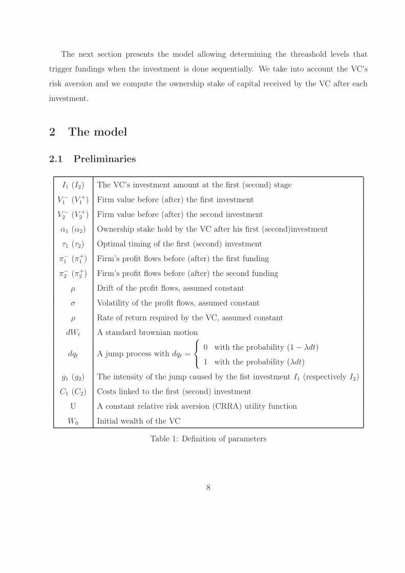
I1 (I2) The VC’s investment amount at the first (second) stage

V −

1 (V +1 ) Firm value before (after) the first investment

V −

2 (V +2 ) Firm value before (after) the second investment

α1 (α2) Ownership stake hold by the VC after his first (second)investment

τ1 (τ2) Optimal timing of the first (second) investment

π−

1 (π+1 ) Firm’s profit flows before (after) the first funding

π−

2 (π+2 ) Firm’s profit flows before (after) the second funding

µ Drift of the profit flows, assumed constant

σ Volatility of the profit flows, assumed constant

ρ Rate of return required by the VC, assumed constant

dWt A standard brownian motion

dqt A jump process with dqt =

0 with the probability (1 − λdt)

1 with the probability (λdt)

g1 (g2) The intensity of the jump caused by the fist investment I1 (respectively I2)

C1 (C2) Costs linked to the first (second) investment

U A constant relative risk aversion (CRRA) utility function

W0 Initial wealth of the VC

Table 1: Definition of parameters

8

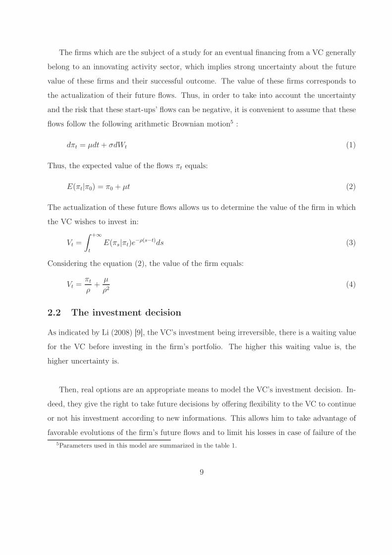
The firms which are the subject of a study for an eventual financing from a VC generally

belong to an innovating activity sector, which implies strong uncertainty about the future

value of these firms and their successful outcome. The value of these firms corresponds to

the actualization of their future flows. Thus, in order to take into account the uncertainty

and the risk that these start-ups’ flows can be negative, it is convenient to assume that these

flows follow the following arithmetic Brownian motion5 :

dπt = µdt + σdWt (1)

Thus, the expected value of the flows πt equals:

E(πt|π0) = π0 + µt (2)

The actualization of these future flows allows us to determine the value of the firm in which

the VC wishes to invest in:

Vt =

∫ +∞

t

E(πs|πt)e−ρ(s−t)ds (3)

Considering the equation (2), the value of the firm equals:

Vt =πt

ρ+

µ

ρ2(4)

2.2 The investment decision

As indicated by Li (2008) [9], the VC’s investment being irreversible, there is a waiting value

for the VC before investing in the firm’s portfolio. The higher this waiting value is, the

higher uncertainty is.

Then, real options are an appropriate means to model the VC’s investment decision. In-

deed, they give the right to take future decisions by offering flexibility to the VC to continue

or not his investment according to new informations. This allows him to take advantage of

favorable evolutions of the firm’s future flows and to limit his losses in case of failure of the

5Parameters used in this model are summarized in the table 1.

9

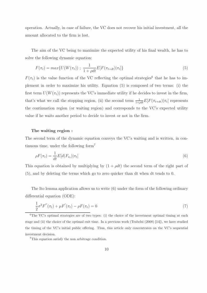
operation. Actually, in case of failure, the VC does not recover his initial investment, all the

amount allocated to the firm is lost.

The aim of the VC being to maximize the expected utility of his final wealth, he has to

solve the following dynamic equation:

F (πt) = max{U(W (πt)) ;1

1 + ρdtE[F (πt+dt)|πt]} (5)

F (πt) is the value function of the VC reflecting the optimal strategies6 that he has to im-

plement in order to maximize his utility. Equation (5) is composed of two terms: (i) the

first term U(W (πt)) represents the VC’s immediate utility if he decides to invest in the firm,

that’s what we call the stopping region, (ii) the second term 11+ρdt

E[F (πt+dt)|πt] represents

the continuation region (or waiting region) and corresponds to the VC’s expected utility

value if he waits another period to decide to invest or not in the firm.

The waiting region :

The second term of the dynamic equation conveys the VC’s waiting and is written, in con-

tinuous time, under the following form7

ρF (πt) =1

dtE[d(Fπt

)|πt] (6)

This equation is obtained by multiplying by (1 + ρdt) the second term of the right part of

(5), and by deleting the terms which go to zero quicker than dt when dt tends to 0.

The Ito lemma application allows us to write (6) under the form of the following ordinary

differential equation (ODE):

1

2σ2F

′′

(πt) + µF′

(πt) − ρF (πt) = 0 (7)

6The VC’s optimal strategies are of two types: (i) the choice of the investment optimal timing at each

stage and (ii) the choice of the optimal exit time. In a previous work (Trabelsi (2008) [14]), we have studied

the timing of the VC’s initial public offering. Thus, this article only concentrates on the VC’s sequential

investment decision.7This equation satisfy the non arbitrage condition.

10

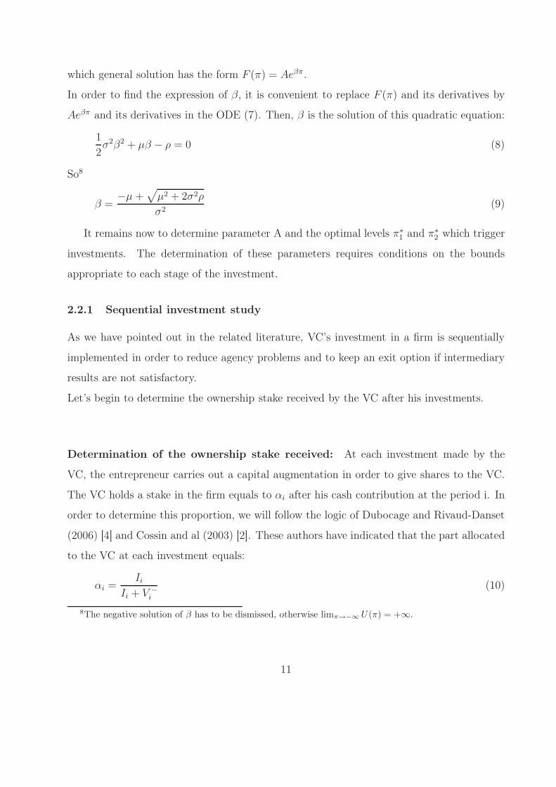
which general solution has the form F (π) = Aeβπ.

In order to find the expression of β, it is convenient to replace F (π) and its derivatives by

Aeβπ and its derivatives in the ODE (7). Then, β is the solution of this quadratic equation:

1

2σ2β2 + µβ − ρ = 0 (8)

So8

β =−µ +

√

µ2 + 2σ2ρ

σ2(9)

It remains now to determine parameter A and the optimal levels π∗

1 and π∗

2 which trigger

investments. The determination of these parameters requires conditions on the bounds

appropriate to each stage of the investment.

2.2.1 Sequential investment study

As we have pointed out in the related literature, VC’s investment in a firm is sequentially

implemented in order to reduce agency problems and to keep an exit option if intermediary

results are not satisfactory.

Let’s begin to determine the ownership stake received by the VC after his investments.

Determination of the ownership stake received: At each investment made by the

VC, the entrepreneur carries out a capital augmentation in order to give shares to the VC.

The VC holds a stake in the firm equals to αi after his cash contribution at the period i. In

order to determine this proportion, we will follow the logic of Dubocage and Rivaud-Danset

(2006) [4] and Cossin and al (2003) [2]. These authors have indicated that the part allocated

to the VC at each investment equals:

αi =Ii

Ii + V −

i

(10)

8The negative solution of β has to be dismissed, otherwise limπ→−∞ U(π) = +∞.

11

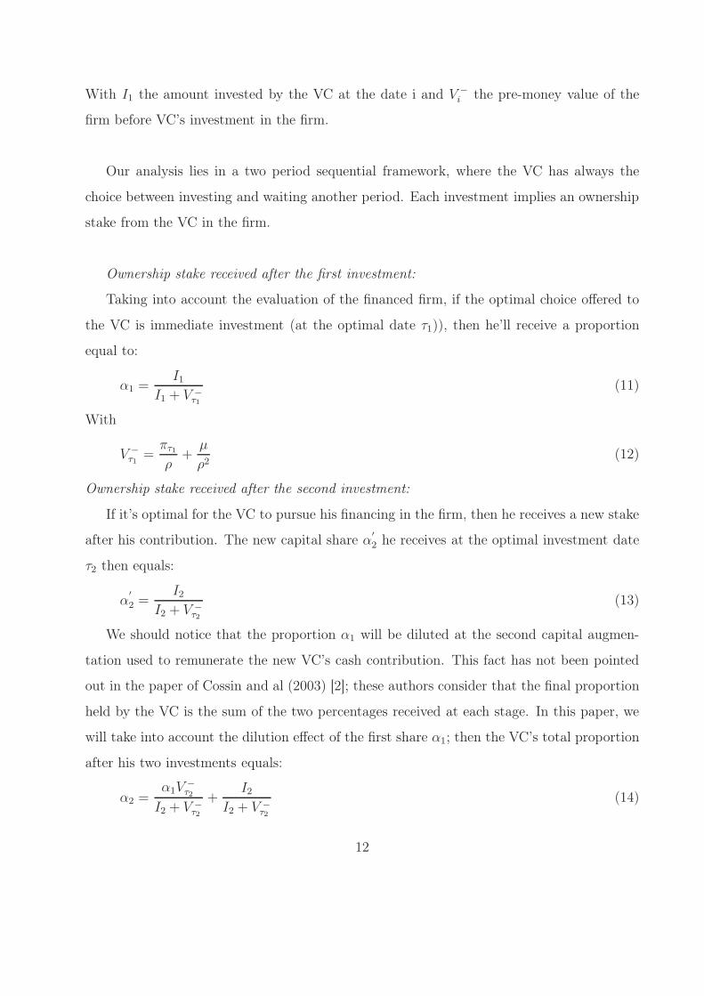
With I1 the amount invested by the VC at the date i and V −

i the pre-money value of the

firm before VC’s investment in the firm.

Our analysis lies in a two period sequential framework, where the VC has always the

choice between investing and waiting another period. Each investment implies an ownership

stake from the VC in the firm.

Ownership stake received after the first investment:

Taking into account the evaluation of the financed firm, if the optimal choice offered to

the VC is immediate investment (at the optimal date τ1)), then he’ll receive a proportion

equal to:

α1 =I1

I1 + V −

τ1

(11)

With

V −

τ1=

πτ1

ρ+

µ

ρ2(12)

Ownership stake received after the second investment:

If it’s optimal for the VC to pursue his financing in the firm, then he receives a new stake

after his contribution. The new capital share α′

2 he receives at the optimal investment date

τ2 then equals:

α′

2 =I2

I2 + V −

τ2

(13)

We should notice that the proportion α1 will be diluted at the second capital augmen-

tation used to remunerate the new VC’s cash contribution. This fact has not been pointed

out in the paper of Cossin and al (2003) [2]; these authors consider that the final proportion

held by the VC is the sum of the two percentages received at each stage. In this paper, we

will take into account the dilution effect of the first share α1; then the VC’s total proportion

after his two investments equals:

α2 =α1V

−

τ2

I2 + V −

τ2

+I2

I2 + V −

τ2

(14)

12

Consequence of each investment on the firm value : The profit flows of the firm are

subject to a positive jump following the arrival of the VC in the capital of the firm. This

jump integrates both the investment made by the VC and the non-financial contribution

of this investor as he is also involved in managing the firm. As a result, after the first

investment, profit flows have to follow this dynamic9 :

dπt = µdt + σdWt + g1dqt (15)

This motion followed by profit flows resembles to an arithmetic Brownian motion with a

positive jump. Thus, after the first investment, the expected value of the firm’s flows π

becomes equal to 10:

E(πs|πτ1) = πτ1 + (µ + g1λ)(s − τ1) (16)

The value of the firm can thus be expressed according to the profit flows:

V +τ1

= E[

∫ +∞

τ1

πse−ρ(s−τ1)ds|πτ1 ] (17)

Using equation (16), the value of the firm V +τ1

after the first financing becomes :

V +τ1

=πτ1

ρ+

µ + g1λ

ρ2(18)

Following the same reasoning to determine the ownership stake α2, we will be located

at this date τ2 which corresponds to the optimal timing of the second investment. At that

date, the present value of the flows (thus the value of the firm) includes the effect of the first

jump. As a consequence, we have to study the effect of this second investment, it means that

we have to take into account the second positive jump of g2 intensity affected the evolution

of the firm’s flows (and the value of the firm). As we did above, this jump also integrates

the new amount of investment I2 and the non-financial contribution of the VC.

The expected flows in the case of no investment are :

E(πs|πt) = πt + µ(s − t) (19)

9The different parameters are defined in the table 1.10E[dWt] = 0, E[dwtdqt] = 0 and E[dqt] = λdt.

13

where πt integrates all the available information until the time t (τ1 < t < τ2). As long as

there is not a new injection of capital from the VC, the firm’s profit flows do not undergo

any jump. As a consequence, at the optimal time τ2, the VC decides to invest a new amount

I2 causing a jump in the value of the firm’s flows whose expected value is :

E(πs|πτ2) = πτ2 + (µ + g2λ)(s − τ2) (20)

The firm value is thus equal to :

V +τ2

=πτ2

ρ+

µ + g2λ

ρ2(21)

As there is no jump between each investment date, the value of the firm just before the

second jump has the same expression as the equation (12) :

V −

τ2=

πτ2

ρ+

µ

ρ2(22)

The expression of the VC’s ownership stake (α2) after his second investment is :

α2 =α1(

πτ2

ρ+ µ

ρ2 ) + I2

I2 +πτ2

ρ+ µ

ρ2

(23)

After having defined the expression of stakes α1 and α2 which are received by the VC if

he invests at the optimal dates τ1 and τ2, it is advisable to determine the utility of VC at

the end of each investment.

2.2.2 The utility of the venture capitalist

The utility function used in this work is of a constant relative risk aversion (CRRA) form.

The general form of this function is U(W ) = 1γW γ which is described by Ingersoll (1987) [8]

and has a constant relative risk aversion equal to ARR = 1 − γ.

The utility of the VC’wealth when he invests in the project the first cash amount I1 at the

optimal time τ1 is :

U1(πτ1) =1

γ[α1V

+(πτ1) − C1 − I1 + W0]γ

14

=1

γ[α1(

πτ1

ρ+

µ + g1λ

ρ2) − C1 − I1 + W0]

γ

=1

γ[

ρI1

ρI1 + πτ1 + µ

ρ

(πτ1

ρ+

µ + g1λ

ρ2) − C1 − I1 + W0]

γ

=1

γ[

I1

(ρI1 + πτ1 + µ

ρ)(πτ1 +

µ + g1λ

ρ) + −C1 − I1 + W0]

γ (24)

In the same way, his utility function at the optimal date of investment τ2 is:

U2(πτ2) =1

γ[α2V

+(πτ2) − C2 − I2 + W0]γ

=1

γ[α1(

πτ2

ρ+ µ

ρ2 ) + I2

I2 +πτ2

ρ+ µ

ρ2

(πτ2

ρ+

µ + g2λ

ρ2) − C2 − I2 + W0]

γ (25)

C1 and C2 represent the cost incurred by the VC when he invests in the project. These

costs are a combination of several costs :

1. Costs related to the search for information which are mainly present in the first phase

of investment. Indeed, being an external investor, VC must draw up several reports

and due diligence11 for well evaluating the prospects for the project and competences

of the managerial team.

2. Costs related to the conclusion of contract and lawyers fees. As indicated by Gompers

(1999) [7], each time an amount is released, a new contract is concluded and adopted,

which increases costs for the VC.

3. Monitoring costs, which are costs, in monetary terms, resulting from the supervision of

entrepreneur, monitoring and counseling of the VC in making decisions and managing

the company. These costs are assumed to be known in advance by the VC.

It should be noted that the costs C1 are greater than C2 as in the second stage of investment,

the VC becomes an insider investor who is more informed than an external investor. Thus,

the costs of search for information are absent (or tiny) at the investment date τ2.

11French association of the investors in capital (AFIC) defines the due diligence as being "the whole

measurements of research and information control allowing the investor to make his opinion on the activity,

the financial standing, the results, the development prospects, the organization of the company."

15

2.2.3 Solving the model

The resolution of the optimal strategy of investment of VC maximizing the equation (5)

results in the determination of the optimal thresholds π∗

1 of investment at date τ1 and π∗

2 of

reinvestment at the time τ2.

The determination of these optimal threshold levels needs the value matching and smooth

pasting conditions. These conditions are specific to each stage of investment.

Value matching and smooth pasting conditions for the first investment

A1eβπ∗

1 = U1(π∗

1) = 1γ[ ρI1ρI1+π∗

1+ µ

ρ

(π∗

1

ρ+ µ+g1λ

ρ2 ) − C1 − I1 + W0]γ

βA1eβπ∗

1 =ρI2

1−I1

g1λ1

ρ

(ρI1+π∗

1+ µ

ρ)2

[ ρI1ρI1+π∗

1+ µ

ρ

(π∗

1

ρ+ µ+g1λ

ρ2 ) − C1 − I1 + W0](γ−1)

(26)

Value matching and smooth pasting conditions for the second investment

A2eβπ∗

2 = 1γ[α1(

π∗

2

ρ+ µ

ρ2)+I2

I2+π∗

2

ρ+ µ

ρ2

(π∗

2

ρ+ µ+g2λ

ρ2 ) − C2 − I2 + W0]γ

βA2eβπ∗

2 = 1

I2+π∗

2

ρ+ µ

ρ2

[1ρ(α1(

π∗

2

ρ+ µ

ρ2 ) + I2) + (π∗

2

ρ+ µ+g2λ

ρ2 )α1I2

ρ−

I2ρ

I2+π∗

2

ρ+ µ

ρ2

]

[α1(

π∗

2

ρ+ µ

ρ2)+I2

I2+π∗

2

ρ+ µ

ρ2

(π∗

2

ρ+ µ+g2λ

ρ2 ) − C2 − I2 + W0](γ−1)

(27)

These two conditions of value-matching and smooth-pasting give :

First threshld relation π∗

1 :

1

β

ρI21 − I1

g1λ1

ρ

(ρI1 + π∗

1 + µ

ρ)2

=1

γ[

ρI1

ρI1 + π∗

1 + µ

ρ

(π∗

1

ρ+

µ + g1λ

ρ2) − C1 − I1 + W0] (28)

16

Second threshold relation π∗

2 :

1

β(

1

I2 +π∗

2

ρ+ µ

ρ2

)[1

ρ(α1(

π∗

2

ρ+

µ

ρ2) + I2) + (

π∗

2

ρ+

µ + g2λ

ρ2)

α1I2ρ

− I2ρ

I2 +π∗

2

ρ+ µ

ρ2

]

=

1

γ[α1(

π∗

2

ρ+ µ

ρ2 ) + I2

I2 +π∗

2

ρ+ µ

ρ2

(π∗

2

ρ+

µ + g2λ

ρ2) − C2 − I2 + W0] (29)

These two equation (28) and (29) are complex, we have to use a numerical solution to

find the value of the critical profit flows that trigger the investment at each stage.

Thus, the optimal investment strategy is to invest as soon as the stochastic flows of the

firm exceeds a threshold level. The trigger of the first investment is made when πt > π∗

1

and the second investment is realized when πt > π∗

2. These two threshold are determined by

solving the two previous systems (27) and (28).

2.3 Numerical application

The aim of this sub section is to test the sensitivity of the threshold values π∗

1 and π∗

2 to the

different parameters used in our model to show that these critical values are in conformity

with the financial logic. Different parameters are varied to test the evolution of the critical

profit flows12.

As we show previously, the VC’s risk aversion is a decreasing function of the parameter

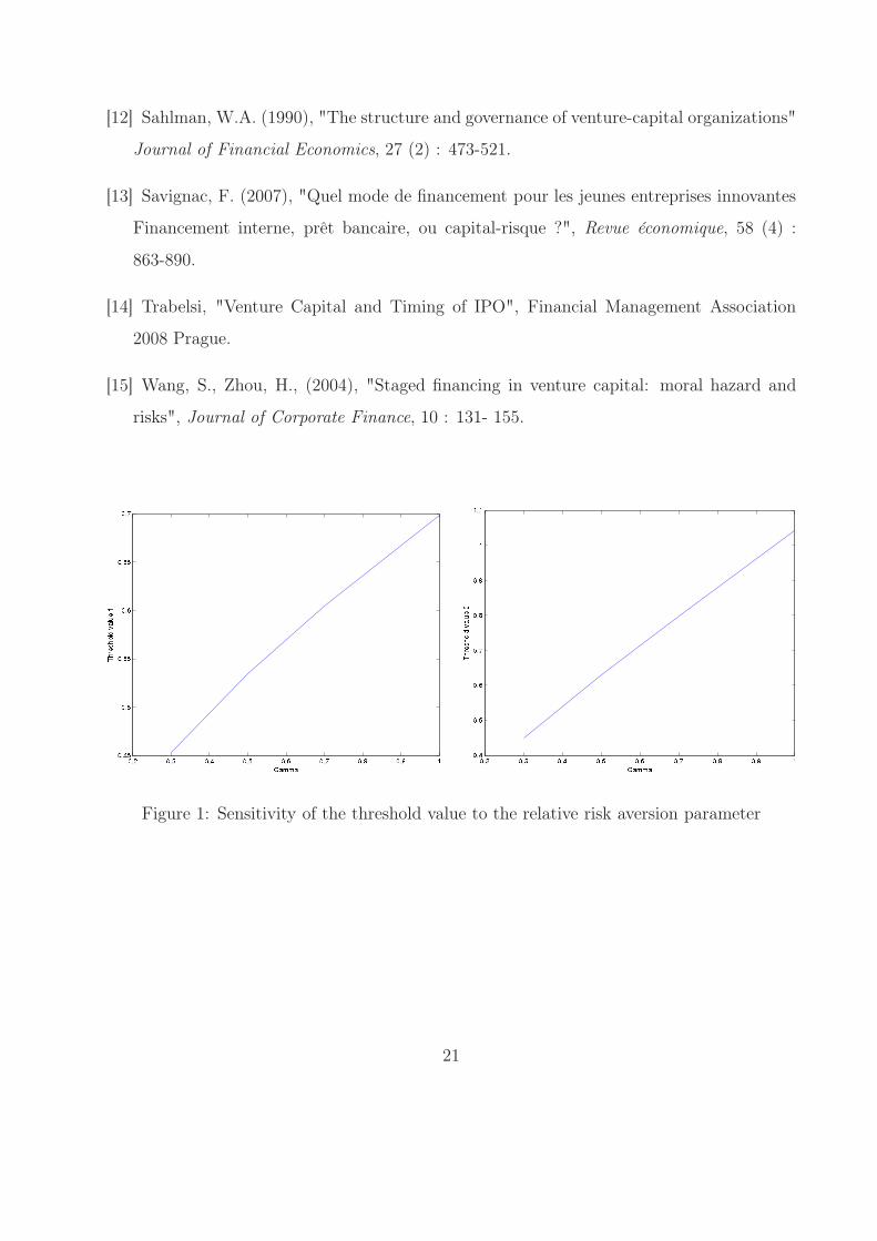
γ, i.e. when γ is high, the VC is less risk averse. The first figure (1) allows us to see

the direction of the variation of the critical values π∗

1 and π∗

2 when the parameter of the

relative risk aversion changes. This graphic shows that, when the risk aversion of the VC

increases (thus, the parameter γ decreases) the threshold value that trigger the investment

(or reinvestment) decreases, which means that the VC invests sooner in the firm to be

financed when he is more risk averse. This can be explained by the fact that this kind of

12The value of parameters used in the numerical application are : γ = 0, 5; µ = 0, 05; σ = 0, 3; ρ = 0, 2;

g1 = g2 = 0, 01; λ = 1; I1 = I2 = 1; W0 = 0, 7; C1 = 0, 5 and C2 = 0, 3.

17

investor prefers investing (or reinvesting) quickly so as to not loose the opportunity that is

offered to him and not to risk the decrease in the value of the project.

The figure (2) shows that the threshold values π∗

1 and π∗

2 increase with the volatility. It’s

clear that a higher level of uncertainty means that the VC will wait a longer period before

he invests (or reinvests) in the firm as it guarantees him a higher return on his investment.

Indeed, a great uncertainty on the profit flows of the firm reduces the motivation of the VC

to invest, which implies an increase in the critical values π∗

1 and π∗

2. This positive relationship

between the threshold value which triggers the investment and the volatility is in conformity

with the results of Dixit and Pindyck (1994) (1994) [3].

The figure (3) shows that the threshold values which activates the investments are a

positive function of the rate of return ρ required by VC. This shows that the waiting period

of the VC before investing in the company is higher as ρ is large. Indeed, for a high level of

the required rate of return, the VC requires a significant proceeds, which increases the value

of the waiting option and delays the investment.

The negative relations between the threshold profit flows values and the growth rate,

the intensity of the jump following the investment as well as the probability of the jump

occurrence are illustrated in the graphs (4), (5) and (6). These graphs are in conformity with

financial logic. In fact, when the parameter µ, g1, g2, λ1 and λ2 increase, the expected profit

flows also increases, which gives more value to the investment and reinvestment opportunity

and to the profits awaited by the VC from his investment in the risky project. The value of

the waiting option will be lower, which encourages the VC to finance the company quickly

as the profit flows become rapidely high.

The graphs (7), (9) and (8) show that the critical values π∗

1 and π∗

2 related to the invest-

ment and the reinvestment are very sensitive to the invested amounts I1 and I2 in each phase

of investment as wall as the initial wealth of the VC W0 and the costs undergone by the VC

(C1 and C2) in each stage of financing. As we can see, when costs ((I and C) increase (or

18

initial wealth drops) the expected profit flows of the company decease and thus the project

has a less value, the VC requires a higher level for profit flows before to be willing to grant

funds to the firm (This relation between the costs and the threshold value is also shown by

Dixit and Pindyck (1994) [3]).

3 Conclusion

In this paper, we considered decision-making investment of a venture capitalist who would

like to finance a risky project in a sequential manner. This means of financing is largely

adopted by the VC as it allows him to reduce his losses and eventual agency problems. In-

deed, if the project’s value decreases after the first investment, the VC can decide to stop

his financing and not to allocate the remaining amount in a project that is not profitable.

The aim of this paper was to determine the different thresholds allowing the VC to re-

ceive a significant capital gain. We first study the ownership stake received by the VC at

each stage of investment, and then we solved the dynamic programming in order to find the

threshold value that trigger the investment. The VC’s investment decision is as follow : at

each stage, the VC invests in the firm if the expected flows of the project are higher than

the critical value.

With a dynamic programming approach, we have determined the levels that trigger the

VC’s investment taking into account his risk aversion, the uncertainty about the future flows

generated by the firm and the ownership stake given to the VC against his financing.

Our numerical results shows that, as expected (dixit and Pindyck (1994) [3]), the (un-

certainty, the rate of return required by the VC, the level of investment, the cost raises the

threshold values required to induce the VC to invest in the firm, which delays the investment

decision. In the same way, the increase in the growth rate the profit flows, the intensity of

the jump and the initial wealth reduce the opportunity cost of waiting, and induce the VC

19

to invest now rather than waiting.

References

[1] Bar-Ilan, A., (2000) "Investment with arithmetic process and lags", Managerial and

decision economics, 21 (5) : 203-206.

[2] Cossin, D., Leleux, B.F., Saliasi, E., "The liquidation preference in venture capital in-

vestment contracts: a real option approach", dans le livre Venture Capital Contracting

and the Valuation of High-Tech Firms, Oxford University Press, 2003, pp318-335.

[3] Dixit, A., Pindyck, R., Investment Under Uncertainty, Princeton University Press, 1994.

[4] Dubocage, E. and Rivaud-Danset D., Le capital-risque, La découverte, 2006.

[5] Giudici, G., Paleari, S., (2000), "The optimal staging of venture capital financing when

entrepreneurs extract private benefits from their firms", Entreprise & Innovation Man-

agement Studies, 1 (2) : 153-174.

[6] Gompers, P.A (1995), "Optimal investment, monitoring, and the staging of venture cap-

ital", The journal of finance, 50 (5) : 1461-1589.

[7] Gompers, P.A., Lerner, J. (1999), Venture capital cycle, MIT Press.

[8] Ingersoll, J.E., Theory of financial decision making, Rowman & Littlefield publishers,

1987.

[9] Li, Y., (2008), "Duration analysis of venture capital staging: A real options perspective",

Journal of Business Venturing, 23 (5) : 497-512.

[10] Poncet, P., Portait, R., Finance de marché : Instruments de base, produits dérivés,

portefeuilles et risques, Dalloz, 2008.

[11] Pouget, J., "Modélisation de la sélection adverse en capital risque par la théorie des

jeux", Association Française de FInance (AFFI) Juin 2007 Bordeaux.

20

[12] Sahlman, W.A. (1990), "The structure and governance of venture-capital organizations"

Journal of Financial Economics, 27 (2) : 473-521.

[13] Savignac, F. (2007), "Quel mode de financement pour les jeunes entreprises innovantes

Financement interne, prêt bancaire, ou capital-risque ?", Revue économique, 58 (4) :

863-890.

[14] Trabelsi, "Venture Capital and Timing of IPO", Financial Management Association

2008 Prague.

[15] Wang, S., Zhou, H., (2004), "Staged financing in venture capital: moral hazard and

risks", Journal of Corporate Finance, 10 : 131- 155.

Figure 1: Sensitivity of the threshold value to the relative risk aversion parameter

21

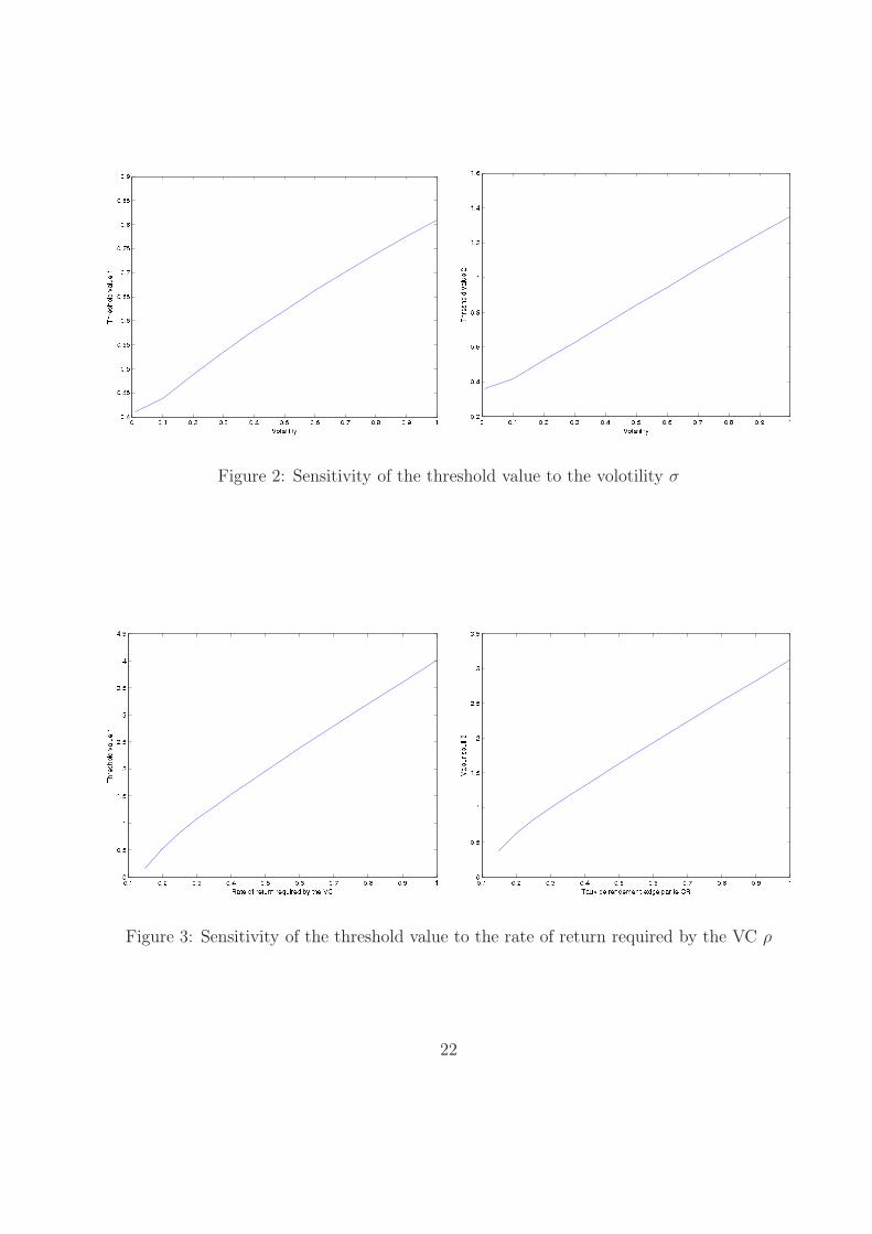
Figure 2: Sensitivity of the threshold value to the volotility σ

Figure 3: Sensitivity of the threshold value to the rate of return required by the VC ρ

22

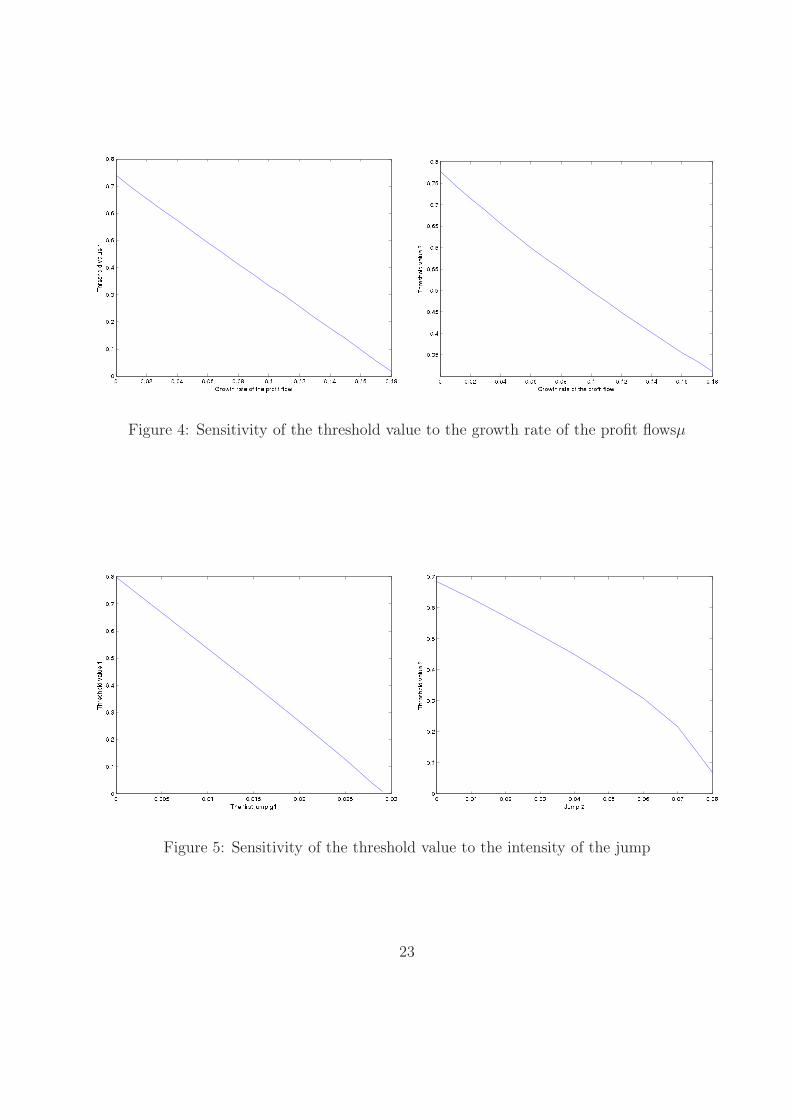
Figure 4: Sensitivity of the threshold value to the growth rate of the profit flowsµ

Figure 5: Sensitivity of the threshold value to the intensity of the jump

23

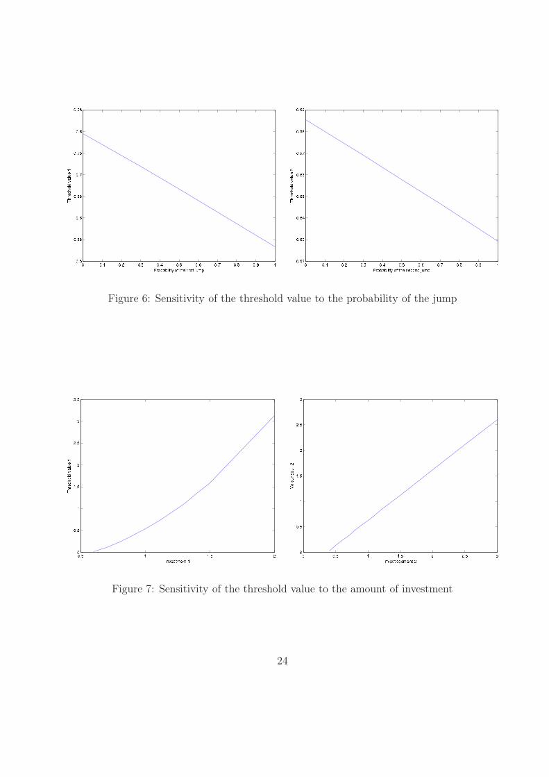
Figure 6: Sensitivity of the threshold value to the probability of the jump

Figure 7: Sensitivity of the threshold value to the amount of investment

24

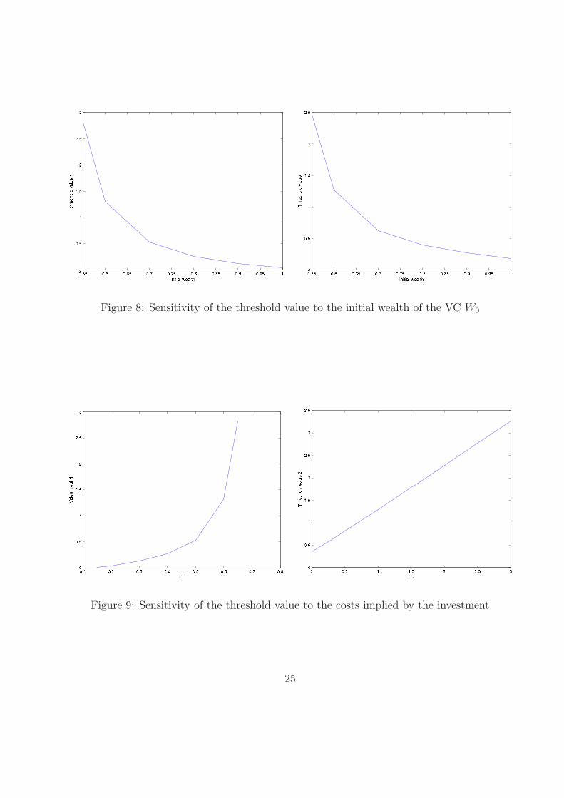
Figure 8: Sensitivity of the threshold value to the initial wealth of the VC W0

Figure 9: Sensitivity of the threshold value to the costs implied by the investment

25