veniamin morgenshtern

Communication Technology Laboratory Communication Theory Group

Capacity scaling in large wireless networks

Veniamin Morgenshtern

Zurich, May 2004

Acknowledgments

I would like to thank my supervisor Prof. Bolcskei for the opportunity to work on

this interesting subject during my stay at the ETH Zurich. I am grateful to him for

fascinating discussions which enforced me to learn a lot about the fundamental

topics in Communication Theory and for freedom he gave me in implementing

my own ideas.

I wish to thank Rohit Nabar for useful discussions we had and for his ideas

which has greatly improved this work.

I want to thank Prof. Terekhov to supervise this work at my home university

in St. Petersburg.

Finally I should say that my life in ETH was really enjoyable! This is due to

the great and warm atmosphere we had inside the Communication Theory Group.

I would like to thank all the members of the group for making my time so fun and

fascinating.

i

ii ACKNOWLEDGMENTS

Abstract

We consider networks consisting of nodes with radios, and without any wired

infrastructure, thus necessitating all communication to take place only over shared

wireless medium. We focus mainly on the flat fading channel model. We study

capacity scaling laws in such systems when the number of nodes gets large. We

show that in extended networks (network with constant density of users) capacity

scales sub-linearly in number of nodes. Thus, when number of nodes gets large,

performance of such system inevitably goes to zero. We show also that in the case

of condensed networks (all the nodes are situated in some bounded area) capacity

can scale super-linearly in the number of nodes. Finally, we present and analyze

particular architecture which achieves capacity bound in the case of condensed

network.

iii

iv ABSTRACT

Contents

Acknowledgments i

Abstract iii

Notations vii

1 Introduction 1

1.1 Overview . . . . . . . . . . . . . . . . . . . . . . . . . . . . . . 1

1.2 Previous results . . . . . . . . . . . . . . . . . . . . . . . . . . . 3

1.3 Contribution . . . . . . . . . . . . . . . . . . . . . . . . . . . . . 3

1.4 Organization of the report . . . . . . . . . . . . . . . . . . . . . . 4

2 Channel and signal model 5

3 Upper bounds 7

3.1 Cut-set bound . . . . . . . . . . . . . . . . . . . . . . . . . . . . 7

3.2 Extended fading networks . . . . . . . . . . . . . . . . . . . . . 8

3.2.1 Uniformly distributed networks . . . . . . . . . . . . . . 8

3.2.2 Bound Based on Hadamard and Jensen Inequalities . . . . 9

3.2.3 Capacity Scaling in Extended Networks . . . . . . . . . . 9

3.2.4 Conclusion . . . . . . . . . . . . . . . . . . . . . . . . . 11

3.3 Condensed networks . . . . . . . . . . . . . . . . . . . . . . . . 11

3.3.1 Cut-set bound in integral form . . . . . . . . . . . . . . . 11

3.3.2 Girko’s law . . . . . . . . . . . . . . . . . . . . . . . . . 12

3.3.3 Capacity Scaling Laws . . . . . . . . . . . . . . . . . . . 13

4 Relay Wireless Networks 19

4.1 Architecture . . . . . . . . . . . . . . . . . . . . . . . . . . . . . 19

4.2 Analysis of the System . . . . . . . . . . . . . . . . . . . . . . . 21

5 Conclusion 27

v

vi CONTENTS

Notations

The superscripts T ,† and ∗ stand for transposition, conjugate transpose, and element-

wise conjugation, respectively. E denotes the expectation operator. Tr(A) and |A|stand for the trace and determinant of the matrix A, respectively. Im stands for

the m × m identity matrix. |X | denotes the cardinality of the set X . The no-

tation u(x) = O(v(x)) denotes that |u(x)/v(x)| remains bounded as x → ∞.

A circularly symmetric complex Gaussian random variable is a random variable

Z = X + j Y ∼ CN (0, σ2), where X and Y are i.i.d. N (0, σ2/2). VAR(X) de-

notes the variance of the random variable X . Throughout the paper all logarithms

unless specified otherwise are to the base 2. AB stands for the Hadamard prod-

uct of matrices A and B.√

A denotes the matrix with components√

Ai,j . The

diagonal matrix with the components of the vector x is denoted by diag(x).

vii

viii NOTATIONS

Chapter 1

Introduction

1.1 Overview

Suppose Alice and Bob are communicating over some channel. In information

theory, channel is usually characterized by conditional probability distribution of

the symbols on the output of the channel, given a symbol on the input. Of course,

real channels are not perfect. This means, for example, that two different symbols

on input can result in a single symbol on the output of the channel because of the

noise or any other causes. That is why if Alice wants to transmit her information

reliably, she needs to use coding. It does not matter what type of coding is used,

the idea remains the same. To send l bits of information to Bob, Alice should

transmit greater number of bits n (n > l) over the channel. Additional bits can

help Bob to recover the initial message. It depends on a particular coding scheme

chosen, how Alice constructs codewords of length n given a message of length l.The ratio R = l/n is usually called the rate of the code. This value is of a great

interest, it characterizes the performance of the particular code. The probability

that Bob has decoded a word that does not coincides with Alice’s message is called

a probability of error. Information theorist and engineers are trying to maximaze

the rate, keeping the probability of error very low. Famous coding theorem (see

[1]) gives a theoretical bound for rate. This bound C is called capacity. Theorem

states that if Alice uses some code with R > C then the probability of error

is inevitably very hight. Reliable communication is impossible on this rate for

any code. On the other hand, if Alice chooses the rate R which is less then C,

then there exists a code which gives infinitely small probability of error. This

means that reliable communication is principally possible. Unfortunatelly, coding

theorem does not describe how to construct such a good code. Capacity is one of

the basic properties of any communication system. It quantifies the quality of the

channel between sender and receiver.

1

2 CHAPTER 1. INTRODUCTION

Consider now several senders and several receivers communicating over wire-

less environment with radios. If all senders and all receivers are transmitting at the

same time in the same frequency band, then they are sharing the same common

media, the same channel. Studying channels with many inputs and many outputs

is the subject of network information theory [2]. Such channels are described by

probability distribution of vectors of outputs, given a vector of inputs. Each user

of the network can principally choose his own rate independently. Thus, network

is fully characterized by the so-called capacity region, i.e. a set of simultaneously

achievable rates. Finding capacity region of the network is very difficult task in

most cases. That is why people often study sum capacity, i.e. the maximum of the

sum of achievable rates. Rather then give complete information about properties

of the channel, sum capacity provides some integral measure. In many papers the

word capacity is used to denote sum capacity. We will also do so for brevity in

the rest of this report.

To compute capacity of the system, one should first model its conditional

probability function. An AWGN (additive channel with Gaussian noise) chan-

nel model is widely used. In this model channel is characterized by the channel

matrix and the noise. The signal vector on input x is first multiplied by channel

matrix G and then noise vector n is added (see Chapter 1 for details):

y = Gx + n.

This model is linear and can be analyzed mathematically more effectively then

other possible models. It is also very natural from the engineering point of view.

The state of the channel, captured by matrix G, can change in time. The

channels which change their state during communication period are called time-

varying or fading. The theory of fading channels have been a subject of intensive

research for many years (see [3] for review) and has many practical applications.

Throughout this work, we focus on fading wireless networks where MS source

terminals are transmitting data to MD destinations terminals. We are particularly

interested in the capacity scaling laws of such networks, i.e. how capacity of the

system grows when MS and MD go to infinity. It is clear, that in order to allow

senders to transmit their data simultaneously on the same rate, capacity should

scale at least linearly with MD. Otherwise achievable rate per sender will go to

zero, when MT ,MD → ∞. Our main goal is to identify situations when desirable

capacity grows can principally be achieved. Once such situations are identified,

we will analyze particular architecture which reaches this bound.

1.2. PREVIOUS RESULTS 3

1.2 Previous results

In his pioneering work [4], Telatar has derived expressions for capacity of MIMO

system (wireless communication system with multiple transmit and receive anten-

nas). He showed that with fixed transmitting power, capacity of the system scales

linearly with number of antennas used. Transmitters and receivers are assumed

to be spatially grouped together, i.e. system can be considered as a condensed

network. To achieve the capacity joint coding and decoding is needed. The results

are achieved for both fading and non-fading case.

For non-fading extended wireless networks first Gupta and Kumar [5] and then

Leveque and Telatar [6] under less restrictive assumptions showed that capacity

can not scale linearly in the number of users. This sets very strong limitation for

possible architectures of large wireless extended networks.

Bolcskei, Nabar, Oyman and Paulraj [7] consider a dense network with fad-

ing and suggest a particular architecture which achieves the theoretical capacity

bound. They assume that the number of transmit terminals is equal to the number

of receive terminals (M = MS = MD). The idea of their approach is to transmit

data through K additional relay terminals, situated between sources and destina-

tions. Communication takes place over two time slots using a one-hop relaying

(”listen-and-transmit”) protocol. During the first time slot M sources simultane-

ously transmit their data to relays. Then the received data is processed by relays

and retransmitted to destination during the second time slot. It is shown in [7]

that for fixed M this architecture achieves capacity C = (M/2) log(K) + O(1)when K is large enough. It is very important that this result is achived without

any cooperation in the system.

1.3 Contribution

The detailed contribution reported in this work can be summarized as follows:

• We explore extended wireless network with fading and prove (under cer-

tain assumptions) that capacity of such network scales sub-linearly with the

number of users. This shows that results by Leveque and Telatar [6] can be

applied for fading networks.

• For condensed networks, we investigate the connection between structure

of channel matrix and an upper bound on the capacity of the system. We

use results from the theory of large random matrices to see how fraction of

active users and network connectivity result capacity bound. We calculate

exact values of the capacity in two special cases.

4 CHAPTER 1. INTRODUCTION

• In paper [7] it is assumed that the number of assisting relays K goes to

infinity, whereas the number of users M remains constant. In this work

we give the analysis of the same protocol for large M limit. We study

relationships between the number of users M and the number of relays Kwhich are needed to assist the transmission. We prove that if number of

relays grows faster than M5 then capacity C = (M/2) log(K) + O(1) is

achieved. The question of what happens when the number of relays grows

slower remains open as a topic for future research.

1.4 Organization of the report

The rest of this report is organized as follows. Chapter II describes the channel

and signal model. In Chapter III, we investigate capacity upper bounds for con-

densed and extended networks and prove corresponding scaling laws. Chapter IV

presents possible network architecture achieving the capacity bound and gives the

analysis in case of large network size. We conclude in chapter V.

Chapter 2

Channel and signal model

We consider a wireless network consisting of MS sending and MD destination

terminals with single antenna each. The sets of all sending and destinations termi-

nals are denoted by S and D respectively. Throughout this report, frequency-flat

fading over the bandwidth of interest is assumed, channel is memoryless. We

will exclusively deal with a linear model in which the received vector y ∈ CMD

depends on the transmitted vector x ∈ CMS via

y = Gx + n

where G = (gij) is the MD ×MS corresponding channel matrix and n is MD × 1circularly symmetric complex white Gaussian noise vector at the receiver with

covariance matrix EnnH = σ2IR. We assume an ergodic block fading channel

model with path-loss such that entries of channel matrix are given by gij = hij ∗√

Eij . H = (hij) is MD × MS matrix consisting of i.i.d. CN (0, 1) entries. It

describes fading in the channel, remains constant over the entire duration of a

time slot and changes in an independent fashion across time slots. MD × MS

matrix E = (Eij) captures path-loss and shadowing in the channel. We assume

that parameters Eij (i = 1, 2, . . . ,MS , j = 1, 2, . . . ,MD) are real, positive, and

remain constant over the entire time period of interest. The exact values will in

general depend on the topology of the network.

Finally, we assume that each transmit terminal is constrained in its total power

P , and uses Gaussian codebooks, that is x is zero-mean MS × 1 circularly sym-

metric complex Gaussian vector satisfying Exx† = PIMS.

5

6 CHAPTER 2. CHANNEL AND SIGNAL MODEL

Chapter 3

Upper bounds

In this chapter, we first apply the well known cut-set bound to the described net-

work and then study the behavior of the derived bound using several methods for

several special cases. This will help us to achieve some intuition on the capac-

ity scaling laws in the general case and give insight on the factors increasing the

capacity.

3.1 Cut-set bound

The cut-set lemma is known to be very general theoretical upper bound on the

network capacity. It has been proved in somewhat different ways for slightly

different setups in the literature ( [2], [4]). We will use the following form of this

lemma.

Lemma 1. The sum of achievable rates of the wireless network modeled with

fading satisfies

C =∑

i∈S,j∈D

Rij ≤ Cupper = EH

log∣

∣IMD+ ρGG†

∣

∣

, (3.1)

where ρ = P/σ2.

Proof. Making a cut between source and destination terminals, using that receiver

knows channel state information, it follows that the capacity of the network is

upper bounded by mutual information

∑

i∈S,j∈D

Rij ≤ I(x; (y,H)).

7

8 CHAPTER 3. UPPER BOUNDS

First using that x is independent of H and then writing mutual information ex-

plicitly we conclude

I (x; (y,H)) = I (x; H) + I (x; y|H) = I (x; y|H) =

= EH

log

∣

∣

∣

∣

IMD+ ρ

(

H √

E)(

H √

E)†∣

∣

∣

∣

.

Substituting G = H √

E we conclude the proof.

It is often very helpful to write down the cut-set bound 3.1 in terms of singular

values of the channel matrix. This is done as follows. Let λi(i = 1, 2, . . . ,MD)be eigenvalues of matrix GG†. Let Λ = diag(λ1 . . . λMD

). Now we can use

eigenvalue decomposition of matrix GG†:

log |IMD+ ρGG†| = log |U−1U + ρU−1

ΛU | = log |U−1(IMD+ ρΛ)U | =

= log |IMD+ ρΛ| = log

MD∏

i=1

(1 + ρλi) =

MD∑

i=1

log (1 + ρλi) .

Substituting this expressions into the cut-set bound (3.1) we receive

Cupper = EH

n∑

i=1

log (1 + ρλi)

. (3.2)

3.2 Extended fading networks

In this section, we apply the general bound (3.1) to extended network, that is

network with constant density of users. Generalizing results reported in [6] by

Leveque and Telatar to fading environment we prove that rate per communication

pair goes to zero when number of users gets large.

3.2.1 Uniformly distributed networks

First, we make additional assumptions on the geometry of the network under con-

sideration. For brevity assume that the number of senders is equal to number of

receivers. Set M = MS = MD. Assume that senders are uniformly distributed

in d-dimensional region ΩSM = [−M1/d, 0] × [0,M1/d]d−1 and receivers are in

the symmetric region ΩDM = [0,M1/d] × [0,M1/d]d−1. The locations of users and

source-destination pairs are chosen once before communication session begins

and remain constant forever. This meets the fact that energy path-loss matrix E is

fixed, which was assumed in the previous chapter.

3.2. EXTENDED FADING NETWORKS 9

For each i ∈ S, | ∈ D let rij denote distance between i-th sender and j-

th receiver. To connect geometrical properties of the network with the model

introduced earlier, we model channel attenuation as follows

Ei,j =e−βri,j

rαi,j

, (3.3)

for all i ∈ S and j ∈ D. Parameter β ≥ 0 is called an absorption constant (usually

positive, unless over a vacuum), and α > 0 is the path loss exponent. This model

is physically motivated and widely used.

In the next subsection we use expression (3.1) to derive weaker but simpler

bound. We then apply it to prove the scaling law for extended wireless network

with fading.

3.2.2 Bound Based on Hadamard and Jensen Inequalities

Starting from formula (3.1) and applying first Hadamard and then Jensen’s we

receive

Cupper = EH

log∣

∣IM + ρGG†∣

∣

≤ EH

logM∏

i=1

(

1 + ρ(GG†)ii

)

≤

≤M∑

i=1

log

(

1 + ρ EH

(GG†)ii

)

.

Note that for each 0 ≤ i ≤ M

EH

(GG†)ii

= EH

M∑

k=1

(G)ik(G†)ki

= EH

M∑

k=1

gikg∗ik

=

=M∑

k=1

EH

∣

∣

∣hki

√

Eki

∣

∣

∣

2

=M∑

k=1

Eki.

Finally

Cupper ≤M∑

i=1

log

(

1 + ρM∑

k=1

Eki

)

. (3.4)

3.2.3 Capacity Scaling in Extended Networks

In this section, we apply bound (3.4) to prove that capacity of the extended wire-

less network of nodes uniformly distributed in the region as described earlier,

almost surely (in respect to spacial distribution) scales sub-linearly in M . We will


transform bound (3.4) in such a way that we can apply results proved by Leveque

and Telatar [6] in the case of networks without fading.

Let us first formulate the results that we are going to use. The facts proved

in [6] can be summarized in the following theorem.

Theorem 1. Let xk (k = 1, 2, . . . , n) be uniformly distributed variables in the

interval [0,M1/d]. Let g(r) = e−βr/2

rα/2 . Let K > 0. Then if β = 0 and α >max(d, 2(d − 2))

1

n

n∑

k=1

log(

1 + K√

ng(xk))

→ 0, n → ∞; (3.5)

if β > 0

1

n

n∑

k=1

log(

1 + Kn2g(xk)2)

→ 0, n → ∞. (3.6)

Convergence in both formulas is almost surely with respect to choice of xk (k =1, 2, . . . , n).

Using notation xi = (x(1)i , x

(2)i , . . . , x

(d)i ) for location of the sender number i

(i = (1, 2, . . . ,M)), substituting (3.3) into (3.4) we deduce:

Cupper ≤M∑

i=1

log

(

1 + ρM∑

k=1

Eki

)

=M∑

i=1

log

(

1 + ρM∑

k=1

g(rki)2

)

≤

≤M∑

i=1

log(

1 + ρMg(x(1)i )2

)

.

(3.7)

Note that x(1)i is uniformly distributed in the interval [0,M1/d]. When β = 0

we write

M∑

i=1

log(

1 + ρMg(|x(1)i |)2

)

≤M∑

i=1

log(

1 + ρM2g(|x(1)i |)2

)

and apply first part of the theorem; when β > 0 we write

M∑

i=1

log(

1 + ρMg(|x(1)i |)2

)

≤ 2M∑

i=1

log(

1 +√

ρMg(|x(1)i |)

)

and apply second part. Finally we conclude that in the case of fading capacity of

extended network scales sub-linearly with the number of users.

3.3. CONDENSED NETWORKS 11

3.2.4 Conclusion

Now we see that in the case of extended network sum capacity can not scale lin-

early with the number of nodes. This implyes that when the size of the network

gets large, performance per each user goes to zero. Thus, some additional tech-

niques should be used to build such networks. One of the possible solutions is

to use wired backbone network as it is done in GSM. In the rest of this work we

focus on condensed networks. In such networks at least some constant fraction of

users stays in the bounded area when the number of users gets large.

3.3 Condensed networks

It is well known that capacity upper bound given by cut-set theorem can be achieved

under certain constraints. For example, it is achieved in MIMO systems when

source and destination terminals can fully cooperate (perform joint coding and

decoding). Sometimes it can also be achieved without cooperation among senders

and receivers. This topic is discussed in the last chapter of this report in more de-

tails. This section is devoted to studying the scaling behavior of the cut-set bound

in condensed networks.

3.3.1 Cut-set bound in integral form

In this subsection, we will transform the upper bound (3.2) into the integral form

in order to apply results from random matrix theory for further analysis. First we

give two important definitions.

Definition 1. Let A be n × n Hermitian matrix. Then FA(x) denotes empirical

eigenvalue distribution of matrix A:

FA(x) =|λ : λ is eigenvalue of A, λ < x|

n.

Definition 2. Function pA(x) = dFA(x)/dx is called density of empirical eigen-

value distribution of matrix A.

Now using formula (3.2) we can write

Cupper = EH

MD∑

i=1

log(1 + ρλi)

= MD EH

1

MD

MD∑

i=1

log(1 + ρλi)

=

MD EH

∫

pGG

†(λ) log (1 + ρλ) dλ

.


It is convenient to normalize matrix G by factor√

MD. Let G = G/√

MD. Let

λi (i = 1, 2, . . . ,MD) denote the eigenvalues of GG†. Then

λi = λi/MD,

dFGG

†(λ) = dFGG

†(λ/MD),

pGG

†(λ)dλ = pGG

†(λ/MD)d(λ/MD),

and changing the variable of integration we conclude

Cupper

MD

= EH

∫

pGG

†(λ) log(1 + ρλ)dλ

=

= EH

∫

pGG

†(λ) log(1 + MDρλ)dλ

.

(3.8)

3.3.2 Girko’s law

The main advantage of studying large networks is that we can apply convergence

results from the theory of large random matrices. These results are somewhat

analogous to the law of large numbers in the classical probability theory. The ba-

sic idea is that in many cases when the size of the random matrix gets large, the

density function of its eigenvalue distribution (which generally is random func-

tion, depending on random matrix) converges almost surely to some non-random

limit. One of the relevant results of this type is due to Girko [8]. It is presented

below.

Theorem 2 (Girko’s law). Let the n × n matrix G be composed of independent

entries gij with zero-mean and variances wij/n such that all wij are uniformly

bounded from above. Assume that the empirical joint distribution of variances

w : [0, 1] × [0, 1] → R defined by wn(x, y) = wij for i, j satisfying

i

n≤ x ≤ i + 1

n,j

n≤ y ≤ j + 1

n

converges to a bounded joint limit distribution w(x, y) as n → ∞. Then, al-

most surely, the empirical eigenvalue distribution of GG† converges weakly to a

limiting distribution whose Stieltjets transform is given by

GGG

†(s) =

∫ 1

0

u(x, s)dx (3.9)

where u(x, s) is a solution of the fixed point equation

u(x, s) =

[

−s +

∫ β

0

w(x, y)dy

1 +∫ 1

0u(x′, s)w(x′, y)dx′

]−1

. (3.10)


The solution to (3.10) exists and is unique in the class of functions u(x, s), Im(u(x, s)) ≥0, analytic for Im(s) > 0 and continuous on x ∈ [0, 1].

Thus, the limiting probability density of eigenvalues of GG† can be computed

by taking the following limit (Stietljes inversion formula):

pGG

†(x) = limy→0+

1

πIm[G(x + iy)]. (3.11)

3.3.3 Capacity Scaling Laws

For simplicity assume again that M = MS = MD. Note that in our notations nor-

malized channel matrix G has independent zero-mean entries gij with variances

Eij/M . From this point on, we assume that the empirical joint distribution of

variances EM(x, y) (see definition in the Girko’s theorem) converges to a bounded

joint limit distribution E(x, y) as M → ∞.

Discussion Let us look briefly at the case of extended networks once again.

Suppose that d = 1. This means that senders are uniformly distributed in the

domain [−M, 0] and receivers are in the domain [0,M ]. Fix any positive distance

r > 0. Let Sr and Dr denote the sets of those source (destination) terminals which

are situated in the regions [−r, 0] and [0, r] respectively. Let SM−r = S \ Sr and

DM−r = D \ Dr. If i ∈ SM−r or j ∈ SN−r, then rij > r and by formula (3.3)

Ei,j <e−βr

rα.

Thus we can see, that

∣

∣

∣

∣

x : EM(x, y) <e−βr

rα∀y ∈ [0, 1]

∣

∣

∣

∣

≈ M − r

M,

∣

∣

∣

∣

y : EM(x, y) <e−βr

rα∀x ∈ [0, 1]

∣

∣

∣

∣

≈ M − r

M.

Setting r =√

M and taking the limit M → ∞ we conclude (when α > 0or β > 0) that almost for all x ∈ [0, 1] the joint limit distribution of variances

E(x, y) = 0 for each y ∈ [0, 1] and vise versa.

If the limiting function E(x, y) exists then it captures all the information about

the capacity of the system. The behavior of E(x, y) described above in the case

of extended networks results in the fact thatCupper

M→ 0.

To compute system capacity given E(x, y) function, we need to solve equa-

tion (3.10), compute Stieltjes transform of the limiting density of eigenvalues by

formula (3.9), apply formula Stilts inversion formula (3.11) to recover the density


of eigenvalues itself, and, finally, substitute this density function into the formula

(3.8) to achieve the upper bound on capacity. Solving equation (3.10) for arbitrary

function E(x, y) seems to be very difficult. That is why we restrict ourselves only

to very specific functions E(x, y) which nevertheless allow to get some intuition

on what is happening in general case.

Model 1: nodes are active partly

Choose 0 ≤ x1 < x2 ≤ 1 and 0 ≤ y1 < y2 ≤ 1. Suppose

E(x, y) =

1, x1 < x < x2 and y1 < y < y2

0, otherwise(3.12)

Denote dx = x2 − x1, dy = y2 − y1. Then fixed point equation (3.10) has the

form1

u(x, s)= −s +

dy

1 +∫ x2

x1u(x′, s)dx′

,

when x ∈ [x1, x2], and the form

1

u(x, s)= −s, (3.13)

when x /∈ [x1, x2].Assume x ∈ [x1, x2]. Supposing that u does not depend on x in this interval:

u(x, s) = v(s) we achieve the following equation on v

1

v= −s +

dy

1 + dxv, (3.14)

or

v2sdx + v(dx − dy + s) + 1 = 0.

Solving this quadric equation, combining the result with solution of (3.13), using

(3.9) and performing the integration we receive

GGG

†(s) = dx

−dx − dy + s

2sdx

+i

2dx

√

4dx

s−(

dx − dy

s+ 1

)2

− 1 − dx

s.

So

pGG

†(x) → limy→0+

1

πIm[G(x + iy)] =

=

12π

√

4dx

x− (dx−dy

x+ 1)2, x ∈ [dy + dx − 2

√

dydx, dy + dx + 2√

dydx]

0, otherwise


almost surely when M → ∞. Finally we only note that limiting empirical eigen-

value distribution pGG

†(x) does not depend on the realization of G. Thus, taking

the expectation in formula (3.8) is trivial and we conclude that

Cupper →

→ M

2π

∫ dy+dx+2√

dydx

dy+dx−2√

dydx

√

2

λ(dx + dy) −

(

dx − dy

λ

)2

− 1 log(1 + ρMλ)dλ

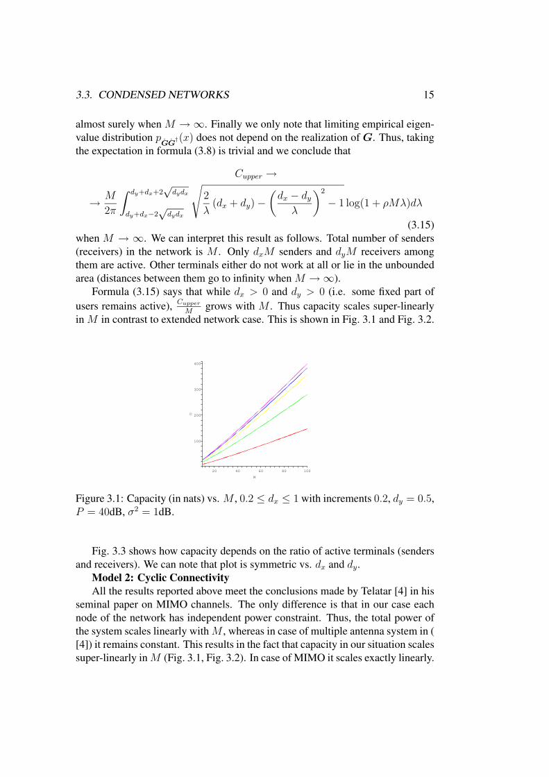
(3.15)

when M → ∞. We can interpret this result as follows. Total number of senders

(receivers) in the network is M . Only dxM senders and dyM receivers among

them are active. Other terminals either do not work at all or lie in the unbounded

area (distances between them go to infinity when M → ∞).

Formula (3.15) says that while dx > 0 and dy > 0 (i.e. some fixed part of

users remains active),Cupper

Mgrows with M . Thus capacity scales super-linearly

in M in contrast to extended network case. This is shown in Fig. 3.1 and Fig. 3.2.

C

300

400

200

M

1008020 6040

100

Figure 3.1: Capacity (in nats) vs. M , 0.2 ≤ dx ≤ 1 with increments 0.2, dy = 0.5,

P = 40dB, σ2 = 1dB.

Fig. 3.3 shows how capacity depends on the ratio of active terminals (senders

and receivers). We can note that plot is symmetric vs. dx and dy.

Model 2: Cyclic Connectivity

All the results reported above meet the conclusions made by Telatar [4] in his

seminal paper on MIMO channels. The only difference is that in our case each

node of the network has independent power constraint. Thus, the total power of

the system scales linearly with M , whereas in case of multiple antenna system in (

[4]) it remains constant. This results in the fact that capacity in our situation scales

super-linearly in M (Fig. 3.1, Fig. 3.2). In case of MIMO it scales exactly linearly.


C

3.5

1.5

4

20

3

1

M

1008040

2

2.5

60

Figure 3.2: Capacity (in nats) divided by M vs. M , 0.2 ≤ dx ≤ 1 with increments

0.2, dy = 0.5, P = 40dB, σ2 = 1dB.

We will now slightly change assumption about behavior of function E and explore

how it results the capacity. Suppose that E is doubly stochastic function, i.e. there

exists constant S such that for each x ∈ [0, 1] and y ∈ [0, 1]

∫ 1

0

E(x′, y)dx′ =

∫ 1

0

E(x, y′)dy′ = S. (3.16)

Function E with this property may appear, for example, if senders and receivers

are uniformly distributed on the concentric circles of the fixed radius. The other

motivation is as follows. In the situation described in the previous section, each

active sender had equally good connection with all of the receivers. This only

can be the case if all senders (and all receivers) are spatially grouped together like

in the multiple antenna systems. If all nodes in the network are active, but each

sender can communicate only to the certain fraction of receivers (other links can

not be established for some reason, for example because corresponding terminals

are too far away from each other) S can be interpreted as a connectivity of the net-

work (i.e relative fraction of receivers with which each sender can communicate).

Cyclic property (3.16) crucially reduces the complexity of Girko equation (3.10)

and allows us to solve it successfully. Assuming again that function u(x, s) does

not depend on x when x ∈ [0, 1]: u(x, s) = v(s), we can write equation on v(s)

1

v(s)= −s +

S

1 + Sv(s).

Solving this equation and following the computations performed earlier (formulas


0

0.20.4

dy

0.60.8

10

0.20.4

0.6 dx0.80

1

100

200

300

400

500

C

600

700

Figure 3.3: Capacity vs. dx and dy, M = 100, P = 40dB, σ2 = 1dB.

(3.14)-(3.15)) we receive

Cupper =M

2π

∫ 4S

0

1

S

√

4S

λ− 1 log(1 + ρMλ)dλ =

=M

2π

∫ 4

0

√

4

λ− 1 log(1 + SρMλ)dλ.

(3.17)

It is very interesting to compare expressions (3.15) and (3.17). First note that

when dx = dy = 1 and S = 1 these two formulas coincide. This is the situation

of MIMO system ( [4]). Note now, that in formula (3.17) parameter S stands

under the logarithm, whereas in formula (3.15) parameters dx and dy determine the

limits of integration and the pre-log. We will see now, that influence of S is much

less then influence of dx and dy in the large M limit. To show this compare two

networks. In the first network 90% of senders and 100% of recievers are active.

Each active node has full connectivity, i.e. it can communicate with all other active

terminal equally well. Mathematically this description corresponds to network of

the first described type with parameters dx = 0.9, dy = 1. Consider now the

second network and suppose that all nodes there are active. At the same time

suppose that each active sender can communicate only with a half of receivers.

This is the network of second type with parameter S = 1/2. Suppose that powers

of terminals and levels of noise are equal in both cases. Denote the capacity of the


first system C1upper and the capacity of the second one C2

upper. Fig. 3.4 shows the

scaling of the difference between these two when M increases. We conclude that

C1-C2

50

40

20

10

0

-20

30

-10M

1000800600400200

Figure 3.4: C2upper − C1

upper in nats vs. M , P = 40dB, σ2 = 1dB.

even thought when values of M are small the influence of small connectivity is

high, when M gets larger the most important factor is the number of active users.

The network with slightly bigger number of active users and with much lower

connectivity has greater capacity (see Fig. 3.4).

Chapter 4

Relay Wireless Networks

In this section we analyse particulary simple ralaying architecture proposed in [7].

The main advantage of this sheme is that it allows to achieve capacity bound

without any cooperation between the terminals in the network (senders, recievers

and relayes). The difference between our analysis and analysis made by Bolcskei,

Nabar, Oyman and Paulraj is that we study the case when number of senders

M → ∞ where as in [7] M is fixed.

4.1 Architecture

Suppose again M = MS = MD. Suppose that before the transmission begins

sources and destinations form communication pairs. Each sourse terminal chooses

exactly one destination terminal which he is going to communicate to. Assume

that between the set of sources S = S1, S2, . . . , SM and the set of destinations

D = (D1, D2, . . . , DM) there is a set of K relay terminals R = (R1, R2, . . . , RK).We assume that K is greater then M and that M devides K. We partition all the

relayes into M disjoint groups:

R = R1 ∪R2 . . . ∪RM

and define a surjective mapping c : K → M using the rule

c(k) = i ⇐⇒ Rk ∈ Ri.

For each i = (1, 2, . . . ,M) the relayes of the group Ri are called assosiated re-

layes of the i-th source-destination pair. As we will see later, assosiated relayes of

the i-th pair establish in fact direct link between Ri and Di cancelling the interfe-

riance of other active terminals.

Suppose that M × K matrix E = (Ei,j) is the energy path-loss matrix of

the channel between sources and relyes; M × K matrix H = (hi,j) is a fading

19

20 CHAPTER 4. RELAY WIRELESS NETWORKS

matrix of the channel between sources and relyes; K × M matrix P = (Pi,j)is energy path-loss in the channel between relayes and destinations, and, finally,

K × M matrix F = (fi,j) is a fading matrix of the channel between relayes and

destinations. K × 1 vector n captures noise on the relayes and M × 1 vector z

describes noise on destinations. Similarly to Chapter 1 we assume that all Ei,j and

Pi,j are strictly positive and bounded from above; hi,j and fi,j are i.i.d. Gaussian;

n and z are Gaussian with variance σ2. To avoid using additional simbols we

assume that senders and relayes are constrained to power P = 1. Relayes and

distanation nodes have full channel state information.

Transmitting protocol consists of two hops. On the first hop, senders simul-

taneously and independently transmit their data to relayes. The signal recived on

k-th relay after the first hop is

rk =M∑

l=1

√

Ek,lhk,lsl + nk, k = 1, 2 . . . , K.

After the first hop relays process the recieved information and prepare it for the

second hop transmition to destinations. Relay number k (assosiated with the

source-destination pair number c(k)) transforms the recieved signal by matched-

filtering it with respect to the channel Sc(k) → Rk, multiplying by energy normal-

ization factor τk and co-phazing with respect to the forward channel Rk → Dc(k)

as follows:

tk =f ∗

c(k),k

|fc(k),k|τkh

∗k,c(k)rk,

where τk = (2Ec(k),k +∑

j 6=c(k) Ej,k + N0)1/2, and tk is the signal after transfor-

mation. Note, that this process does not require big computational effort (relayes

do not need to decode the signal). Nevertheless, relayes need to know both input

and output channels.

Finally, the m-th destination node recieves

ym =K∑

k=1

√

Pm,kfm,ktk + zl =

=K∑

k=1

√

Pm,kfm,k

f ∗c(k),k

|fc(k),k|uk + zm =

=K∑

k=1

√

Pm,kfm,k

f ∗c(k),k

|fc(k),k|τkh

∗k,c(k)rk + zm =

=K∑

k=1

√

Pm,kfm,k

f ∗c(k),k

|fc(k),k|τkh

∗k,c(k)

(

L∑

l=1

√

Ek,lhk,lsl + nk

)

+ zm,

(4.1)

4.2. ANALYSIS OF THE SYSTEM 21

m = (1, 2, . . . ,M).

4.2 Analysis of the System

We assume that each destinations terminal decodes its massage separatelly, with-

out any cooperation with others. He needs to separate the message adressed to

him of messages adressed to other user of the network (interference). We rewrite

expression (4.1) separating signal, interference, and noise contributions:

ym =K∑

k=1

M∑

l=1

τk

√

Pm,kEk,lfm,k

f ∗c(k),k

|fc(k),k|h∗

k,c(k)hk,lsl+

+K∑

k=1

√

Pm,kfm,k

f ∗c(k),k

|fc(k),k|τkh

∗k,c(k)nk + zm =

=sm(∑

k∈Rm

τk

√

Pm,kEk,m|fm,k||hk,m|2+

+∑

k/∈Rm

τk

√

Pm,kEk,lfm,k

f ∗c(k),k

|fc(k),k|h∗

k,c(k)hk,m)+

+∑

l 6=m

sl

K∑

k=1

τk

√

Pm,kEk,l|fm,k|h∗k,mhk,l+

+K∑

k=1

√

Pm,kfm,k

f ∗c(k),k

|fc(k),k|τkh

∗k,c(k)nk + zm.

(4.2)

To simplify this expresion we introduce the notations

dm,lk = τk

√

Pm,kEk,lgm,k

g∗c(k),k

|gc(k),k|hk,lh

∗k,c(k),

and

fmk = τk

√

Pm,kgm,k

g∗c(k),k

|gc(k),k|h∗

k,c(k).

Now we can rewrite the signal recieved by m-th destination terminal in the fol-

lowing form:

ym =sm

(

∑

k∈Rm

dm,mk +

∑

k/∈Rm

dm,mk

)

+∑

l 6=m

sl

K∑

k=1

dm,lk +

K∑

k=1

fmk nk + zm.


Recalling that we assumed independent encoding and decoding and full channel

knowledge we can now write expresion for the capacity of this system [7]:

Clower =M∑

i=1

EE,F

Ii (4.3)

where

Ii =1

2log (1 + SINRi)

is mutual information between i-th sender and i-th reciever and

SINRi =ES

i

EN+Ii

=|∑k∈Rm

dm,mk +

∑

k/∈Rmdm,m

k |2∑

l 6=m |∑Kk=1 dm,l

k |2 + σ2∑K

k=1 |fmk |2 + σ2

.

is the corresponding signal to noise plus interference ratio.

We are now going to find such conditions on M and K, that it is possible

to bound SINRi from below. Building the uniform lower bound for all SINRi

(i = 1, 2, . . . ,M ) we build lower bound on the capacity which scales at least

lineary in M .

We are going to use Chebyshev’s inequality to estimate SINRi.

Theorem 3 (Chebyshev’s inequality). Let X1, X2, . . . , Xn be independent ran-

dom variables with means µ1, µ2, . . . , µn and variances σ21, σ

22, . . . , σ

2n respec-

tively. Let S = X1 + . . . + Xn, µ = µ1 + . . . + µn, and σ2 = σ21 + . . . + σ2

n. Then

for any t

Pr |S − µ| > tσ ≤ 1

t2.

To use this theorem we first compute means and variances of dm,lk and fm

k with

respect to H and F .

First we compute expectations:

E

dm,lk

=

0, k /∈ Lm or m 6= l√

Pm,kEk,m

2Ec(k),k+P

j 6=c(k) Ej,k+N0E |gm,k| , k ∈ Lm,m = l;

(4.4)

E

|fmk |2

=Pm,k

2Ec(k),k +∑

j 6=c(k) Ej,k + N0

. (4.5)

Now compute variances:

V AR(

dm,lk

)

=Pm,kEk,l

2Ec(k),k +∑

j 6=c(k) Ej,k + N0E

|hk,lh∗k,c(k)|2

−(

E

dm,lk

)2

;

(4.6)


V AR(

|fmk |2)

=

=

(

Pm,k

2Ec(k),k +∑

j 6=c(k) +N0

)2

E

|gm,kg∗c(k),k|4

|gc(k),k|4|h∗

k,c(k)|4

−(

E

|fmk |2)2

.

(4.7)

Then, applying Chebyshev’s inequality for each of the sums separately we

conclude that probability of each of the following events is t−2 or less:

∣

∣

∣

∣

∣

K∑

k=1

dm,mk −

∑

k∈Rm

E dm,mk

∣

∣

∣

∣

∣

≥ t

√

√

√

√

K∑

k=1

V AR (dm,mk );

when l 6= m∣

∣

∣

∣

∣

K∑

k=1

dm,lk

∣

∣

∣

∣

∣

≥ t

√

√

√

√

K∑

k=1

V AR(

dm,lk

)

;

and∣

∣

∣

∣

∣

K∑

k=1

|fmk |2 −

K∑

k=1

E |fmk |2∣

∣

∣

∣

∣

≥ t

√

√

√

√

K∑

k=1

V AR (|fmk |2).

Note that we have M2 + M inequalities here. For each of these inequalities,

the probability of that it is satisfied is less then t−2. Resume that for any events

A1, A2, . . . , An

Pr (A1 ∪ A2 ∪ . . . ∪ An) ≤n∑

i=1

Pr(Ai).

Using this for M2 + M inequalities we conclude that probability of that at least

one of them is satisfied is less then M2+Mt2

. Finally, we conclude that probability

of that no one of these inequalities is satisfied (i.e. all opposite inequalities are

satisfied all together) is greater then 1 − M2+Mt2

. From this point on we assume

that this is fullfield.

Then, the following bounds on signal and noise-interference energy can be

written for each m, n and i simultaneously:

ESi ≥

max

0,∑

k∈Rm

E dm,mk − t

√

√

√

√

K∑

k=1

V AR (dm,mk )

2

, (4.8)


EN+Ii ≤

≤∑

l 6=m

t2K∑

k=1

V AR(

dm,lk

)

+ σ2

K∑

k=1

E

|fmk |2

+ t

√

√

√

√

K∑

k=1

V AR (|fmk |2) + 1

.

(4.9)

Now we will simplify these expretions by uniformly bounding variances and

mean values in them. We recall that the network is bounded and there is some min-

imal separation distance between nodes. This means that there are constants 0 <P∗ ≤ P ∗ and 0 < E∗ ≤ E∗ such that P∗ ≤ Pi,j ≤ P ∗ and E∗ ≤ Ei,j ≤ E∗. Using

the following notations for brevity: A1 = E |gm,k|, A2 = E

|hk,lh∗k,c(k)|2

and

A3 = E

|gm,kg∗c(k),k

|4

|gc(k),k|4 |h∗

k,c(k)|4

, from formulas (4.4), (4.5), (4.6), and (4.7) we

deduce

E dm,mk ≥

√

P∗E∗

E∗(M + 1) + N0

A1,

E

|fmk |2

≤ P ∗

E∗(M + 1) + N0

,

V AR(

dm,lk

)

≤ P ∗E∗

E∗(M + 1) + N0

A2,

V AR(|fmk |2) ≤

(

P ∗

E∗(M + 1) + N0

)2

A3.

Substituting these expressions into (4.8) and (4.9) we conclude that

ESi ≥

≥(

max

[

0, |Rm|√

P∗E∗

E∗(M + 1) + N0

A1 − t

√

KP ∗E∗

E∗(M + 1) + N0

A2

])2

,

EN+Ii ≤

≤ (M − 1)t2KP ∗E∗A2

E∗(M + 1) + N0

+ σ2

(

KP ∗

E∗(M + 1) + N0

+t√

KP ∗A3

E∗(M + 1) + N0

+ 1

)

,

and

SNIRi ≥(

max[

0, |Rm|√

P∗E∗A1 − t√

KP ∗E∗A2

])2

(M − 1)t2KP ∗E∗A2 + σ2(KP ∗ + t√

KP ∗A3 + E∗(M + 1) + N0).

(4.10)

Finally, suppose that K = Mγ . We want to choose parameter γ in such a way

that right hand side of (4.10) does not go to zero when M → ∞ almost surely


with respect to G and F . We know that the relayes are equally distributed among

the source destination pairs, i.e. |Rm| = Mγ−1 for each m = (1, 2, . . . ,M). Now

set t2 = (L2 + L)δ. Substitute the values of t and R into formula (4.10) and

ommit terms of lower order in M . We conclude the following. Simalteniously for

all i = (1, 2, . . . ,M) with probability at least 1 − 1δ

assimptotically in M

SNIRi ≥M2(γ−1)P∗E∗

Mγ+3δP ∗E∗A2

=Mγ−5P∗E∗

δP ∗E∗A2

.

This proves the following lemma.

Lemma 2. There exists constant Q such that for any δ > 0

Pr

SNIRi ≥ QMγ−5

δ∀i = (1, 2, . . . ,M)

≥ 1 − 1

δ.

From this lemma and formula (4.3) we achieve the main theorem.

Theorem 4. Suppose number of relayes K = Mγ . Then there exists a constant Qsuch that for any δ > 0

Pr

Clower ≥M

2log

(

1 + QMγ−5

δ

)

≥ 1 − 1

δ.

When γ > 5 this theorem sais that capacity of the system scales superlinearly

in M .

Chapter 5

Conclusion

In this work we have compared capacity scaling laws for different wireless sys-

tems over Gaussian channels with fading. We have shown that in the case of

extended networks, capacity scales sublinearly in the number of terminals. This

may serve as a hint on thumb for engeneers. It is not likely that the extended net-

work can be built without backbone wired infrastructure. We have studyed several

types of condensed networks and have shown how relayes can be used to assist

communication in such cases. We should note that the bound γ = 5 given in the

lust section does not seem to be tight. We are currently working on improving

this bound. If we manage to do so, this will mean that less relayes are needed for

reliable transmission in the described network.

27

28 CHAPTER 5. CONCLUSION

Bibliography

[1] R. G. Gallager, Information Theory and Reliable Communication, Wiley,

1968.

[2] T. M. Cover and J. A. Thomas, Elements of Information Theory, Wiley, New

York, 1991.

[3] E. Biglieri, J. Proakis, and S. Shamai, “Fading channels: Information-

theoretic and communications aspects,” IEEE Transactions on Information

Theory, vol. 44, no. 6, pp. 2619–2692, Oct. 1998.

[4] I. E. Telatar, “Capacity of multi-antenna Gaussian channels,” European

Transactions on Telecommunications, vol. 10, pp. 585–595, Nov./Dec. 1999.

[5] P. Gupta and P. R. Kumar, “The capacity of wireless networks,” IEEE Trans-

actions on Information Theory, vol. 46, no. 2, pp. 388–404, Mar. 2000.

[6] O. Leveque and E. Telatar, “Information theoretic upper bounds on the capac-

ity of large extended ad-hoc wireless networks,” submitted to IEEE Transac-

tions on Information Theory, Feb 2004.

[7] H. Bolcskei, R. Nabar, O. Oyman, and A. Paulraj, “Capacity scaling laws

in mimo relay networks,” presented in part at the Allerton Conference on

Communications, Control, and Computing, Monticello, IL, Oct. 2003.

[8] Vjaceslav L. Girko, Theory of Random Determinants, Kluwer Academic

Publishers, Dordrecht, The Netherlands, 1990.

29

veniamin morgenshtern

Documents