velocity smoothing before depth migration: does it help or ... · salt allows systematic analysis...

CWP-512

Velocity smoothing before depth migration: Does it

help or hurt?

Ken Larner and Carlos PachecoCenter for Wave Phenomena, Colorado School of Mines, Golden, CO 80401

ABSTRACT

Previous studies of the sensitivity of depth migration to smoothing of themigration-velocity model have treated smoothing of an initially correct model.Aside from the relatively small amount of smoothing that is needed for imagingwith Kirchhoff migration and that does no harm to imaging with finite-differencemigration, smoothing of the model changes the model from the true one, sothose studies have shown the less smoothing the better. Because we never knowthe subsurface velocity function with perfect accuracy, imaging is always com-promised to some extent by error in the migration-velocity model. Given thatreality, perhaps some amount of smoothing of the inevitably erroneous velocitymodel could improve quality of the migrated image.We have performed a number of tests of imaging with erroneous velocity mod-els for a simple synthetic 2D model of reflectors beneath salt. The salt layerhas a chirp-shape boundary so that we could assess imaging quality as a func-tion of lateral wavelength of velocity variation in the overburden. Errors thatwe introduce into the velocity model include lateral and vertical shifting ofthe chirp-shape (usually top-of-salt) boundary, and erroneous amplitude of thechirp, including random errors in the chirp shape. Primarily with poststackmigration of modeled exploding-reflector, we assess sub-salt image quality formigrations with many different smoothings of erroneous velocity models. Wefind that, depending on the type and size of error in the shape of the top-of-saltboundary, as well as the lateral wavelength of the chirp, smoothing of the er-roneous velocity model before migration can benefit image quality, sometimessubstantially. The form of error that can most benefit from smoothing is errorin the shape, as opposed to position, of the salt boundary. This observation,based on numerous tests with exploding-reflector data, is supported by a smallnumber of tests with smoothing of the erroneous velocity model in prestackmigration.

Key words: velocity smoothing, depth migration

1 INTRODUCTION

No factor is of larger importance to imaging quality indepth migration than accuracy of the velocity modelused for the migration. Velocity information, however, isinevitably erroneous to some extent. Finding sufficientlyaccurate velocity for migration is an especially difficulttask in complex regions such as beneath salt in the Gulfof Mexico, an impediment to efficient exploration anddevelopment there (Paffenholz, 2001).

Because information about the spatial variationof subsurface velocity can never be known in detail,in practice estimated velocities are routinely smoothedover space prior to using them for migration. More-over, because Kirchhoff-type migration algorithms ob-tain their traveltime information from some form of raytracing, the velocities used must be spatially smoothedto insure stability in the ray computations.

Any smoothing changes the subsurface velocitymodel and hence the migration result, so too much

198 K. Larner & C. Pacheco

smoothing will certainly lead to distortion in migratedimages. Of importance, then, is to know how muchsmoothing of the migration velocity field becomes toomuch.

Various studies, notably those of Versteeg (1993),Gray (2000), and Paffenholz et al. (2001), have aimedat providing guidance on the appropriate amount ofspatial smoothing of velocity for depth migration. Acommon conclusion of those studies, all of which in-volved smoothing of known velocities in complex two-dimensional (2D) synthetic datasets such as the Mar-mousi, Sigsbee2, and SEG-EAGE salt models, is thatthe appropriate amount of smoothing is both model-and depth-dependent. The study of Gray (2000), whichfocused on Kirchhoff migration, found that, althoughsome smoothing is necessary for that approach, “too lit-tle smoothing produced a better image than too muchsmoothing” because too much smoothing will changethe velocity model substantially, perhaps to the extentof removing geologic plausibility.

Because Versteeg (1993) did his migrations with awavefield-migration approach, which had no dependenceon ray tracing, smoothing of the velocity was not essen-tial to overcome a deficiency of the migration method.Paralleling a conclusion of Jannane et el. (1989), Ver-steeg argued that the velocity model need not includespatial wavelengths smaller than an amount governedby the wavelengths for frequencies in the data, withfurther dependence on the complexity of the velocitymodel. His tests showed that smoothing of the knownvelocity model up to a certain amount (about 200 mfor realistic frequencies in the Marmousi data set) wasquite acceptable.

In their migration tests with the Sigsbee2 model,Paffenholz et al. (2001) demonstrated the clear supe-riority of wavefield migration (e.g., finite-difference mi-gration) over Kirchhoff migration when the migrationvelocity model is known perfectly, but “the advantageof wavefield migration disappears if the (salt) velocitycontains errors.” They also showed degradation in sub-salt imaging when the migration-velocity model used iserroneous, either because of error in the shape of thesalt or because smoothing of the correct model is toolarge to some extent.

In all of the studies mentioned above, the testswith smoothing for migration involved smoothing of theknown, true velocity model. Recall, however, that oneof the reasons for smoothing is that we cannot knowthe true velocity structure in detail – and sometimes wehave rather poor information about the velocity struc-ture. It therefore is appropriate to conduct studies inwhich the smoothing is applied not to the known, cor-rect velocity model but to models that are erroneous.Then, depending on complexity of the velocity model,amount of error in that model, depth of target beneaththe erroneous overburden, and frequency content in thedata, some degree of smoothing is likely optimal in the

sense of yielding a better image of the target than is useof either less or more smoothing.

In the study here, we perform migrations withsmoothed versions of erroneous velocity models andmake a start at answering the question “does smoothingof the erroneous velocity field help or hurt the qualityof the migrated result?”

As in the references mentioned above, our testsmake use of synthetic data. Most of our models, how-ever, are much more simple than those in the publishedstudies, with little attempt to mimic realistic subsurfacestructure. We introduce errors in the shape of the mod-eled salt and migrate the data when different degrees ofspatial smoothing are applied to the erroneous velocitymodels.

In order to perform enough tests to draw generalconclusions here, most of tests entail 2D modeling andmigration. Moreover, for reasons discussed below, mostinvolve poststack migrations of data generated underthe exploding-reflector assumption.

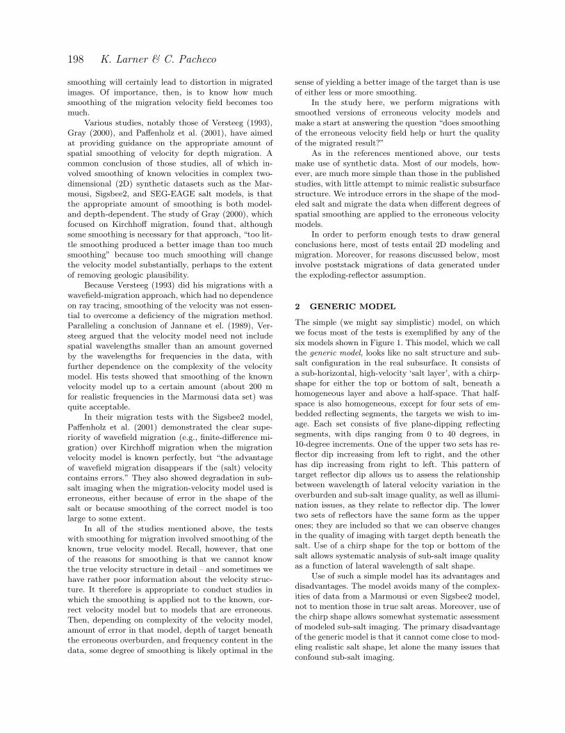
2 GENERIC MODEL

The simple (we might say simplistic) model, on whichwe focus most of the tests is exemplified by any of thesix models shown in Figure 1. This model, which we callthe generic model, looks like no salt structure and sub-salt configuration in the real subsurface. It consists ofa sub-horizontal, high-velocity ‘salt layer’, with a chirp-shape for either the top or bottom of salt, beneath ahomogeneous layer and above a half-space. That half-space is also homogeneous, except for four sets of em-bedded reflecting segments, the targets we wish to im-age. Each set consists of five plane-dipping reflectingsegments, with dips ranging from 0 to 40 degrees, in10-degree increments. One of the upper two sets has re-flector dip increasing from left to right, and the otherhas dip increasing from right to left. This pattern oftarget reflector dip allows us to assess the relationshipbetween wavelength of lateral velocity variation in theoverburden and sub-salt image quality, as well as illumi-nation issues, as they relate to reflector dip. The lowertwo sets of reflectors have the same form as the upperones; they are included so that we can observe changesin the quality of imaging with target depth beneath thesalt. Use of a chirp shape for the top or bottom of thesalt allows systematic analysis of sub-salt image qualityas a function of lateral wavelength of salt shape.

Use of such a simple model has its advantages anddisadvantages. The model avoids many of the complex-ities of data from a Marmousi or even Sigsbee2 model,not to mention those in true salt areas. Moreover, use ofthe chirp shape allows somewhat systematic assessmentof modeled sub-salt imaging. The primary disadvantageof the generic model is that it cannot come close to mod-eling realistic salt shape, let alone the many issues thatconfound sub-salt imaging.

Velocity smoothing before depth migration 199

M1 M2

M3 M4

M5 M6

Figure 1. Velocity models M1-M6 used to generate the synthetic data. Lateral position is denoted by x, and depth by z.

Simple as it is, the generic model nevertheless ischaracterized by enough parameters that comprehensivestudy of imaging would require a large number of testsof models with many different combinations of valuesfor those parameters. Parameters of the generic modelinclude

• average depth of the top and bottom of the salt• velocities of the salt and of the layers above and

below• parameters of the chirp-shape top or bottom of salt,

specifically

– amplitude of the chirp– range of spatial wavelengths of the chirp

• target depths

Our study can only spottily cover the large combi-


0 2 4 6 8 10 12 14 16 18 20500

1000

1500

2000

2500

3000

3500

4000

4500

x (km)

λ (m

)

Figure 2. Range of spatial wavelengths for the two chirpsused in our study. The solid line shows wavelength λ as afunction of lateral position for models M1, M2, and M5; thedashed line shows wavelength for models M3, M4, and M6.

nation of pertinent values for these many parameters.Moreover, none of the six models in Figure 1 exhibitsthe large structural size of the salt in, for example, theSigsbee2 model. So, the study is a mere start.

When we consider the different forms of error inthe velocity models and differing amounts of smoothingof those erroneous models, the number of tests to per-form could further multiply greatly. Errors could arisein all of the parameters (except for the sub-salt reflectordescription) listed above. For example, the chirp-shapetop of salt used for the migration-velocity model couldbe shifted laterally or vertically from the true position,or have erroneous amplitude.

Our tests with the generic model all involve thesix models in Figure 1. All six have velocities of 2000m/s, 4500 m/s, and 3500 m/s for the top layer, saltlayer, and half-space, respectively. For all six models, theaverage depth of the top and bottom of the salt is 1000m and 1900 m, respectively. Models M1, M2, and M5have the same range of spatial wavelength for the chirp,and Models M3, M4, and M6 have a higher range ofspatial wavelength. The variation of spatial wavelengthwith horizontal location is shown in Figure 2. Otherdifferences among the six models are in the amplitudeof the chirp shape. Table 1 summarizes the parametervalues for the chirp in each model.

Another important parameter for the tests wouldbe the range of frequencies contained in the seismicwavelet used in the wavefield modeling. All of our testsinvolve just one choice of input wavelet – a Rickerwavelet, with dominant frequency of 15 Hz.

model λmax (m) λmin (m) h (m) top bottom

M1 2500 500 50 X

M2 2500 500 100 X

M3 4500 1000 100 X

M4 4500 1000 200 X

M5 2500 500 50 X

M6 2500 500 100 X

Table 1. Chirp parameters for the generic velocity modelused in the study. The parameter h is the ampliitude of thechirp, i.e., the peak departure of salt-boundary depth fromits average value.

3 ZERO-OFFSET VERSUS

EXPLODING-REFLECTOR DATA

Ultimately one might prefer that a study of the sensitiv-ity of sub-salt imaging to errors in the velocity modelbe done with 3D prestack depth migration applied tomodeled 3D data. The cost of such a study is clearlyprohibitive, certainly in this decade. Among the manyother complexities of such a study would be the issue ofhow to define a useful 3D extension of the chirp model.

Our study therefore is strictly limited to 2D. Even2D prestack depth migration imposes too large a com-putational cost for other than a small number of to-ken comparison tests with the generic model. In orderto do enough comparisons, we limited the study pri-marily to imaging with poststack migration. The sim-plification doesn’t stop here, however. We can envisionthree different forms of input to poststack migration:(1) modeled data from many source-to-receiver offsetsthat have been stacked, (2) zero-offset (ZO) data ex-tracted from normal-moveout-corrected and unstackedmodeled data, and (3) exploding-reflector (ER) modeleddata. We did tests with all three forms, but the largestnumber with exploding-reflector data.

The choice of exploding-reflector data may seempuzzling. One reason for this choice is that generation ofER data is least computationally costly. We use a finite-difference code, second-order in time, fourth-order inspace, for the modeling; the cost of modeling zero-offsetdata would be essentially the same as that of modelinga full prestack data set. But there is another reason forchoosing exploding-reflector data over extracted zero-offset data.

Seismic data that result from ER modeling arelargely equivalent to, but differ in important respectsfrom, either ZO or common-midpoint (CMP) stackeddata, particularly in the presence of strong lateral veloc-ity variation (Kjartasson & Rocca, 1979) and (Spetzler& Snieder, 2001). Moreover, the pattern of multiples and


the relative amplitudes of the primaries and multiplesdiffer among the three forms of data.

So, why do we consider a study using ER data tobe useful? Because poststack migration is based on theexploding-reflector assumption, such migration of zero-offset data would be erroneous even if the migration ve-locity were correct. In contrast, because poststack (i.e.,zero-offset) migration and exploding-reflector modelingof primaries are essentially exact inverses of one another,we can count on accurate migration of ER primarieswhen we use the correct migration velocities. Therefore,sensitivity of imaging to errors in velocity, includingsmoothing of erroneous velocity, is best isolated whenwe apply poststack migration to ER data.

That ER and ZO data differ from one another, asdo the results of poststack migration applied to thesetwo forms of data, is exhibited in Figures 3 and 4. Thedifferences between the ER and ZO sections for modelsM1, M2, and M4, in Figure 3, are striking. Particularlyfor models with larger chirp amplitude and in regionsof the model with smaller chirp wavelength, sub-saltreflections show more numerous triplications character-istic of caustics and multi-pathing in the overburden.The exploding-reflector sections exhibit less loss of am-plitude with time and more complete expression of thediffractions than do the zero-offset sections. Since mi-gration aims to collapse diffractions, the distorted andincomplete diffractions in the ZO data will be poorlycollapsed in poststack-migrated results. The strongeramplitudes at late time in the ER data result from theweaker geometric spreading from sources that are, in ef-fect, placed on the exploding reflectors than the spread-ing from the surface line sources for the ZO data. Fi-nally, as expected, the timing and amplitudes of multi-ples in the exploding-reflector sections differ from thosein the counterpart zero-offset sections. The multiplesin these data are internal ones. Surface multiples arelargely absent because absorbing boundary conditions(Clayton & Engquist, 1977) were used for all bound-aries.

The results of poststack (i.e., zero-offset) depth mi-gration of the exploding-reflector and zero-offset sec-tions using the true velocity for the migration are shownin Figure 4, again for models M1, M2, and M4. Weused an f-x domain, finite-difference depth-migration al-gorithm (Claerbout, 1985) for both migrations. For allmodels, depth migration of the exploding-reflector datayields high-quality imaging of the primaries, with arti-facts related to migration of the multiples. In contrast,depth migration of the zero-offset sections results in de-graded imaging of the sub-salt reflectors, especially inregions of the model where the chirp has smaller wave-length. Since these migrations were performed using thecorrect velocity model, the compromised migrated ZOdata offer a poor starting point for study of sub-saltimaging when smoothed, erroneous velocity models areused for the migration.

Using equation (12) of Spetzler and Snieder (2004),we calculated approximate focal depths (depths atwhich caustics and triplications start to appear) for thesix velocity models used in the study. Although onlyroughly approximate because that equation assumes1D lateral slowness variations and point sources, thesecomputed focal depths give a measure of the relativecomplexity of the various models and of wavefields inthem. For our generic models, this complexity, whichdepends on the depth and lateral variation of the veloc-ity anomaly, is controlled mainly by the geometry of thechirp. Figure 5 shows the focal depths below the surfaceas a function of lateral position x for the six chirp mod-els. Model M2, for example, has caustics that appearat the shallowest depth, whereas caustics arise deeperfor the models with milder chirp shape, and for chirpshape at the base rather than the top of the salt. Therelatively poor image, in Figure 4, of the migrated zero-offset data for Model 2, as compared with the migratedimages for models M1 and M4, suggests dependence ofimage quality on model complexity. (Again, the imagingproblem arises because zero-offset migration is based onthe exploding-reflector idea.) Also, as seen in Figure 5,the levels of complexity of models M1 and M4 are equiv-alent. Consistent with this observation, the image qual-ity of the depth-migrated zero-offset sections for thesemodels is comparable.

When errors are present in the velocity model, the degradation of migrated ER data will differ fromthat in (1) poststack-migrated ZO data, (2) prestack-migrated ZO data, and (3) prestack-migrated full-offsetdata. Even with the correct velocity model the quality ofimaging can be compromised in each of these treatmentsof data. We’ve already seen in Figure 4 that, becausepoststack migration is founded on the ER assumption,poststack-migrated ZO data is erroneous even when thecorrect velocity model is used for migration. Prestack-migrated ZO data do not suffer from that shortcoming,but can exhibit image distortion and artifacts arisingfrom insufficient pre-migration muting of wide-angle re-flections and refractions prior to the migration, limitedaperture for the (shot-record) migration, and variationsin wavefield illumination beneath the salt. Prestack-migrated, full-offset data can also be distorted becauseof variable illumination, insufficient muting, and limitedmigration aperture. These data, however, have the ad-vantage that the worst of these problems are mitigatedto some extent by destructive interference of offset-dependent distortions and artifacts after stacking themigrated data for all offsets.

4 LENGTH SCALES FOR VELOCITY

SMOOTHING

For finite-difference migration, if we knew the velocitymodel perfectly we would have no need to smooth thevelocities. Smoothing could only alter the model from


M1

0

1

2

3

4

time

(s)

0 2 4 6 8 10 12 14 16 18 20x (km)

0

1

2

3

4

time

(s)

0 2 4 6 8 10 12 14 16 18 20x (km)

M2

0

1

2

3

4

time

(s)

0 2 4 6 8 10 12 14 16 18 20x (km)

0

1

2

3

4

time

(s)

0 2 4 6 8 10 12 14 16 18 20x (km)

M4

0

1

2

3

4

time

(s)

0 2 4 6 8 10 12 14 16 18 20x (km)

0

1

2

3

4

time

(s)

0 2 4 6 8 10 12 14 16 18 20x (km)

Figure 3. Exploding-reflector sections (left) and zero-offset sections (right) for models M1, M2, and M4.

the true one, resulting in erroneous migration — themore smoothing the poorer the image. Versteeg (1993),however, showed that there is little harm done with anamount of spatial smoothing that is small in relation tothe wavelengths in the signal and fineness of detail inthe velocity model. Even for Kirchhoff migration, Gray(2000) pointed out that smoothing too little is betterthan smoothing too much.

Before addressing smoothing of erroneous velocitymodels, let us see how much smoothing of our correctgeneric models is acceptable for the depth migration.Given the range of complexities suggested for the modelsin Figure 5, we expect that the appropriate amount ofsmoothing will differ from one model to another.

We smooth the velocity functions using a two-dimensional Gaussian-shaped operator similar to the


M1

0

2000

4000

6000

dept

h (m

)

0 2 4 6 8 10 12 14 16 18 20x (km)

0

2000

4000

6000

dept

h (m

)

0 2 4 6 8 10 12 14 16 18 20x (km)

M2

0

2000

4000

6000

dept

h (m

)

0 5 10 15 20x (km)

0

2000

4000

6000

dept

h (m

)

0 2 4 6 8 10 12 14 16 18 20x (km)

M4

0

2000

4000

6000

dept

h (m

)

0 5 10 15 20x (km)

0

2000

4000

6000

dept

h (m

)

0 2 4 6 8 10 12 14 16 18 20x (km)

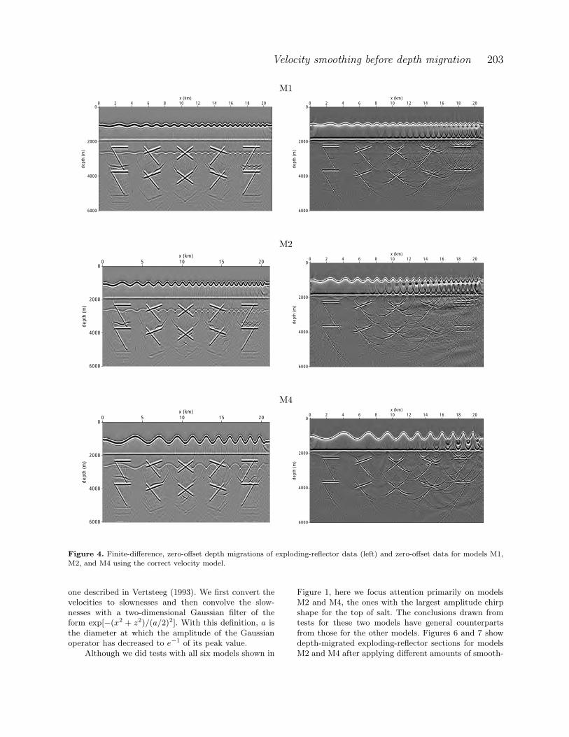
Figure 4. Finite-difference, zero-offset depth migrations of exploding-reflector data (left) and zero-offset data for models M1,M2, and M4 using the correct velocity model.

one described in Vertsteeg (1993). We first convert thevelocities to slownesses and then convolve the slow-nesses with a two-dimensional Gaussian filter of theform exp[−(x2 + z2)/(a/2)2]. With this definition, a isthe diameter at which the amplitude of the Gaussianoperator has decreased to e−1 of its peak value.

Although we did tests with all six models shown in

Figure 1, here we focus attention primarily on modelsM2 and M4, the ones with the largest amplitude chirpshape for the top of salt. The conclusions drawn fromtests for these two models have general counterpartsfrom those for the other models. Figures 6 and 7 showdepth-migrated exploding-reflector sections for modelsM2 and M4 after applying different amounts of smooth-


2 4 6 8 10 12 14 16 18

1000

2000

3000

4000

5000

6000

x (km)

zca

us (m

)

M1M2M3M4M5M6

Figure 5. Focal depths zcaus for the velocity models in Fig-ure 1. We associate shallower focal depth with larger modelcomplexity.

ing to the correct velocity model. Not surprising, as thedegree of smoothing increases, the quality of the im-aged sub-salt reflectors worsens; for any given amountof smoothing, the degradation is model-dependent. Themore complex the overburden model (i.e., the shallowerthe computed focal depth shown in Figure 5), the fasterthe image degrades with increased smoothing. Thus, fora given amount of smoothing, the degradation for modelM2 is more severe than that for model M4. For both,the degradation is worse beneath the shorter-wavelengthportion of the chirp. For these two models, the maxi-mum smoothing diameter that yields acceptable imag-ing is about 160 m. For the remaining models, a smooth-ing diameter of 200 m, and even larger, yields acceptableimaging of the target reflections.

The models in which the bottom rather than thetop of the salt has the chirp shape can be smoothedas much as 400 m without introducing significant dis-tortion of the imaged sub-salt reflections. One reasonfor this is the closer proximity of the chirp boundary tothe targets. Another is that the impedance contrast, andconsequently the lateral velocity variation, is smaller forthe models with chirp-shape bottom rather than top ofthe salt.

We note that our observations and impressions ofimage quality are subjective, based on assessment offour characteristics of imaged reflectors: their locations,sharpness of imaged events, distortion in imaged reflec-tor shape, and contaminating artifacts.

As seen especially in Figure 7, the deeper targetssuffer somewhat larger distortion than do the shallowerones. The farther waves have propagated through thevelocity model the more complicated they become. Keepin mind that it is not the complexity of the velocitymodel directly above a reflector that influences the qual-ity of imaging, but rather the complexity along the dom-inant ray directions. Thus the steep reflectors on theright side of the figures are better imaged than are the

horizontal ones. Conversely, the horizontal reflectors atthe left are better imaged than are the dipping onesthere.

Another aspect of smoothing, seen in Figure 8, aregaps in the imaged bottom of the salt for model M2migrated using velocities smoothed with a=160 m. Thesmoothed velocity model does not have the detail nec-essary to honor all the ray bending and multi-pathingthat occurs at the chirp interface. As a result, migratingwith the smoothed velocity model creates illuminationgaps in the bottom-of-salt reflection.

To summarize, for migration with finite-differences,smoothing of the true velocity model can only degradethe imaging quality; it cannot improve it. For the genericvelocity models with chirp-shape top of salt, the maxi-mum amount of smoothing that produces an acceptablydepth-migrated image is that with a ≈ 200 m. Thismaximum acceptable smoothing, however, depends onthe complexity of the model. In agreement with the re-sults of Versteeg (1993) and Gray (2000), the less com-plex the model, the more smoothing that is acceptable.Again, however, in practice we cannot know the veloc-ity model in detail. Next we investigate what happenswhen we smooth erroneous velocity models.

5 SMOOTHING OF ERRONEOUS

VELOCITY MODELS:

EXPLODING-REFLECTOR DATA

Here, we again consider poststack depth migration ofexploding-reflector data generated for the generic veloc-ity models. We first migrate using the erroneous velocitymodel and then repeat the migration after applying dif-ferent amounts of smoothing to the erroneous velocitymodel. We introduced errors of the following kind to thegeneric velocity models:

• lateral and vertical shifts of the chirp-shape top orbottom salt boundary,

• erroneous amplitude of the chirp-shape boundary,• random perturbations added to the chirp,• erroneous velocity of the salt layer.

As simple as is our generic velocity model, the listof model parameters shown in Section 3, plus all thescale lengths (Fresnel zone, chirp wavelength, smooth-ing diameter, scale length of the velocity error, depthof the targets) involved in the problem make systematicanalysis of depth migration for different smoothings oferroneous migration velocities a large task. We showonly a few selected examples that illustrate main obser-vations of the study.

The benefit or harm done by velocity smoothingdepends on the type of error. For migration of field datain practice, velocity models will have a combination ofall the forms of error that we introduce individually inthis study.


true a = 80 m

0

2000

4000

6000

dept

h (m

)

0 5 10 15 20x (km)

0

2000

4000

6000

dept

h (m

)

0 5 10 15 20x (km)

a = 160 m a = 240 m

0

2000

4000

6000

dept

h (m

)

0 5 10 15 20x (km)

0

2000

4000

6000

dept

h (m

)

0 5 10 15 20x (km)

a = 320 m a = 400 m

0

2000

4000

6000

dept

h (m

)

0 5 10 15 20x (km)

0

2000

4000

6000

dept

h (m

)

0 5 10 15 20x (km)

Figure 6. Depth-migrated exploding-reflector sections for model M2 using the correct velocity model and after different amountsof smoothing have been applied to that correct model. The diameter of the two-dimensional Gaussian smoothing operator isdenoted by a.

Some types error in the velocity model have rela-tively small influence on the migrated image. For ex-ample, vertical shifts of the salt boundary and constanterror in the velocity of the sediments surrounding thesalt body have relatively little influence on sub-salt im-age quality. These two types of error primarily causeerror in reflector depth without severely distorting or

defocusing the image. Pon and Lines (2004) and Paf-fenholz et al. (2001) obtained similar results with theirmodeled data sets. Smoothing of these erroneous veloc-ity models has much the same influence on the quality ofimaging as does smoothing of the correct velocity mod-els. Increasing the degree of smoothing in this case onlyfurther degrades image quality.


true a = 80 m

0

2000

4000

6000

dept

h (m

)

0 5 10 15 20x (km)

0

2000

4000

6000

dept

h (m

)

0 5 10 15 20x (km)

a = 160 m a = 240 m

0

2000

4000

6000

dept

h (m

)

0 5 10 15 20x (km)

0

2000

4000

6000

dept

h (m

)

0 5 10 15 20x (km)

a = 320 m a = 400 m

0

2000

4000

6000

dept

h (m

)

0 5 10 15 20x (km)

0

2000

4000

6000

dept

h (m

)

0 5 10 15 20x (km)

Figure 7. Same as Figure 6, but for model M4.

In contrast, consistent with the results of Paffenholzet al., we find that lateral shift of the chirp model cancause significant degradation of sub-salt imaging, as doerrors in the geometry of the chirp boundary. In general,a given amount of lateral shift of the boundary causeslarger degradation of the sub-salt image than does acomparable vertical shift.

As we shall see, where error in the velocity modelcauses substantial degradation of the migrated image.smoothing the erroneous velocity model can improvethe quality of the migrated image. Where it causes toosevere degradation, once again no smoothing can help.


0

500

1000

dept

h (m

)

0 1 2 3 4 5 6x (km)

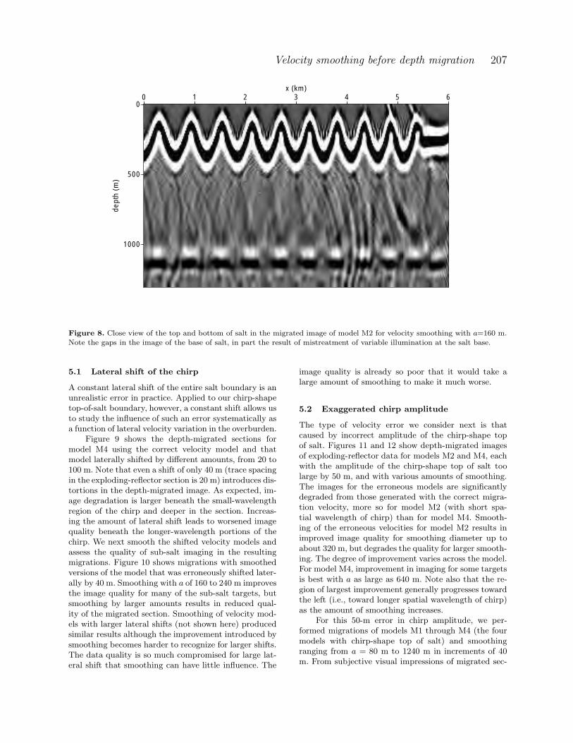
Figure 8. Close view of the top and bottom of salt in the migrated image of model M2 for velocity smoothing with a=160 m.Note the gaps in the image of the base of salt, in part the result of mistreatment of variable illumination at the salt base.

5.1 Lateral shift of the chirp

A constant lateral shift of the entire salt boundary is anunrealistic error in practice. Applied to our chirp-shapetop-of-salt boundary, however, a constant shift allows usto study the influence of such an error systematically asa function of lateral velocity variation in the overburden.

Figure 9 shows the depth-migrated sections formodel M4 using the correct velocity model and thatmodel laterally shifted by different amounts, from 20 to100 m. Note that even a shift of only 40 m (trace spacingin the exploding-reflector section is 20 m) introduces dis-tortions in the depth-migrated image. As expected, im-age degradation is larger beneath the small-wavelengthregion of the chirp and deeper in the section. Increas-ing the amount of lateral shift leads to worsened imagequality beneath the longer-wavelength portions of thechirp. We next smooth the shifted velocity models andassess the quality of sub-salt imaging in the resultingmigrations. Figure 10 shows migrations with smoothedversions of the model that was erroneously shifted later-ally by 40 m. Smoothing with a of 160 to 240 m improvesthe image quality for many of the sub-salt targets, butsmoothing by larger amounts results in reduced qual-ity of the migrated section. Smoothing of velocity mod-els with larger lateral shifts (not shown here) producedsimilar results although the improvement introduced bysmoothing becomes harder to recognize for larger shifts.The data quality is so much compromised for large lat-eral shift that smoothing can have little influence. The

image quality is already so poor that it would take alarge amount of smoothing to make it much worse.

5.2 Exaggerated chirp amplitude

The type of velocity error we consider next is thatcaused by incorrect amplitude of the chirp-shape topof salt. Figures 11 and 12 show depth-migrated imagesof exploding-reflector data for models M2 and M4, eachwith the amplitude of the chirp-shape top of salt toolarge by 50 m, and with various amounts of smoothing.The images for the erroneous models are significantlydegraded from those generated with the correct migra-tion velocity, more so for model M2 (with short spa-tial wavelength of chirp) than for model M4. Smooth-ing of the erroneous velocities for model M2 results inimproved image quality for smoothing diameter up toabout 320 m, but degrades the quality for larger smooth-ing. The degree of improvement varies across the model.For model M4, improvement in imaging for some targetsis best with a as large as 640 m. Note also that the re-gion of largest improvement generally progresses towardthe left (i.e., toward longer spatial wavelength of chirp)as the amount of smoothing increases.

For this 50-m error in chirp amplitude, we per-formed migrations of models M1 through M4 (the fourmodels with chirp-shape top of salt) and smoothingranging from a = 80 m to 1240 m in increments of 40m. From subjective visual impressions of migrated sec-


true shift=20 m

0

2000

4000

6000

dept

h (m

)

0 5 10 15 20x (km)

0

2000

4000

6000

dept

h (m

)

0 5 10 15 20x (km)

shift=40 shift=60 m

0

2000

4000

6000

dept

h (m

)

0 5 10 15 20x (km)

0

2000

4000

6000

dept

h (m

)

0 5 10 15 20x (km)

shift=80 shift=100 m

0

2000

4000

6000

dept

h (m

)

0 5 10 15 20x (km)

0

2000

4000

6000

dept

h (m

)

0 5 10 15 20x (km)

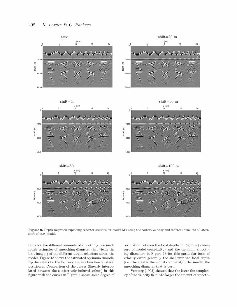
Figure 9. Depth-migrated exploding-reflector sections for model M4 using the correct velocity and different amounts of lateralshift of that model.

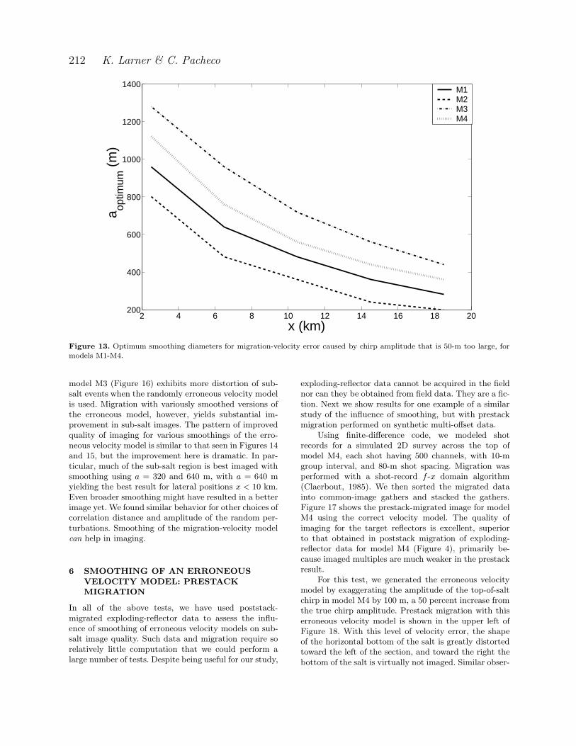
tions for the different amounts of smoothing, we maderough estimates of smoothing diameter that yields thebest imaging of the different target reflectors across themodel. Figure 13 shows the estimated optimum smooth-ing diameters for the four models, as a function of lateralposition x. Comparison of the curves (linearly interpo-lated between the subjectively inferred values) in thisfigure with the curves in Figure 5 shows some degree of

correlation between the focal depths in Figure 5 (a mea-sure of model complexity) and the optimum smooth-ing diameters in Figure 13 for this particular form ofvelocity error: generally the shallower the focal depth(i.e., the greater the model complexity), the smaller thesmoothing diameter that is best.

Versteeg (1993) showed that the lower the complex-ity of the velocity field, the larger the amount of smooth-


true shifted

0

2000

4000

6000

dept

h (m

)

0 5 10 15 20x (km)

0

2000

4000

6000

dept

h (m

)

0 5 10 15 20x (km)

a = 80 m a = 160 m

0

2000

4000

6000

dept

h (m

)

0 5 10 15 20x (km)

0

2000

4000

6000

dept

h (m

)

0 5 10 15 20x (km)

a = 240 m a = 320 m

0

2000

4000

6000

dept

h (m

)

0 5 10 15 20x (km)

0

2000

4000

6000

dept

h (m

)

0 5 10 15 20x (km)

Figure 10. Depth-migrated exploding-reflector sections for model M4 using the correct velocity model, for that model laterallyshifted by 40 m, and for various degrees of smoothing applied to the laterally shifted model.

ing of the velocity model that is acceptable for imaging.Here, we find a counterpart result: the lower the com-plexity of the velocity field, the larger the amount ofsmoothing that yields the best imaging when the ini-tial model is in error. In tests with larger error in chirpamplitude (100-m too large), we found a similar corre-

lation between model complexity and optimum amountof smoothing.

5.3 Random perturbation of the chirp

The final type of error in the migration-velocity modelthat we show is a random perturbation of the chirp-


true erroneous

0

2000

4000

6000

dept

h (m

)

0 5 10 15 20x (km)

0

2000

4000

6000

dept

h (m

)

0 5 10 15 20x (km)

a=160 m a=320 m

0

2000

4000

6000

dept

h (m

)

0 5 10 15 20x (km)

0

2000

4000

6000

dept

h (m

)

0 5 10 15 20x (km)

a=480 m a=640 m

0

2000

4000

6000

dept

h (m

)

0 5 10 15 20x (km)

0

2000

4000

6000

dept

h (m

)

0 5 10 15 20x (km)

Figure 11. Depth-migrated exploding-reflector sections for model M2 with true velocity, for an erroneous velocity model causedby chirp amplitude exaggerated by 50 m (a 50 percent exaggeration), and for smoothed versions of the erroneous velocity model.

shape top of the salt. We distorted the shape by adding alaterally bandlimited, Gaussian-distributed depth errorto the chirp. For the test results shown in Figures 14, 15,and 16, the correlation length l = 100 m, where l is thelag at which the autocorrelation of the random depthvariation decreases by a factor e−1 of its peak value. Thecorrelation length is a measure of lateral scale length of

velocity error. For these tests, the standard deviation ofthe random depths prior to bandlimiting is σ = 50 m.

Figures 14 and 15 show migrated sections usingthe true velocity model, a model with random erroradded to the depth of the chirp, and variously smoothedversions of the erroneous velocity function for modelsM2 and M4. For both models, migration with the erro-


true erroneous

0

2000

4000

6000

dept

h (m

)

0 5 10 15 20x (km)

0

2000

4000

6000

dept

h (m

)

0 5 10 15 20x (km)

a=160 m a=320 m

0

2000

4000

6000

dept

h (m

)

0 5 10 15 20x (km)

0

2000

4000

6000

dept

h (m

)

0 5 10 15 20x (km)

a=480 m a=640 m

0

2000

4000

6000

dept

h (m

)

0 5 10 15 20x (km)

0

2000

4000

6000

dept

h (m

)

0 5 10 15 20x (km)

Figure 12. Same as Figure 11 but for model M4. The 50-m increase in chirp amplitude represents a 25 percent exaggerationof the amplitude for this model.

neous velocity function yields severely distorted imagingof the sub-salt reflections. For model M2 (Figure 14),which has the shorter-wavelength chirp-shape top ofsalt, smoothing of the erroneous velocity model yields,at best, marginal improvement, with optimal smoothingvarying from a = 160 m to at least 640 m for reflectorsfrom right to left. The improvement brought about bysmoothing the erroneous model is more evident in the

results for model M4, shown in Figure 15. As smooth-ing increases from a = 160 m to 640 m, targets thatare best imaged again are those beneath progressivelylonger-wavelength portions of the chirp.

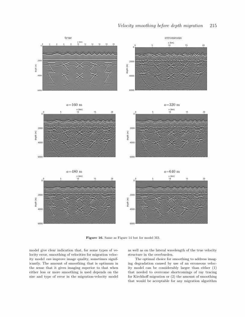
Model M3 has chirp shape spanning the same rangeof wavelengths as those in model M4, but with smaller-amplitude chirp. Compared to results for similarly con-sidered models M2 and M4, migration for data from


2 4 6 8 10 12 14 16 18 20200

400

600

800

1000

1200

1400

x (km)

a optim

um (m

)

M1M2M3M4

Figure 13. Optimum smoothing diameters for migration-velocity error caused by chirp amplitude that is 50-m too large, formodels M1-M4.

model M3 (Figure 16) exhibits more distortion of sub-salt events when the randomly erroneous velocity modelis used. Migration with variously smoothed versions ofthe erroneous model, however, yields substantial im-provement in sub-salt images. The pattern of improvedquality of imaging for various smoothings of the erro-neous velocity model is similar to that seen in Figures 14and 15, but the improvement here is dramatic. In par-ticular, much of the sub-salt region is best imaged withsmoothing using a = 320 and 640 m, with a = 640 myielding the best result for lateral positions x < 10 km.Even broader smoothing might have resulted in a betterimage yet. We found similar behavior for other choices ofcorrelation distance and amplitude of the random per-turbations. Smoothing of the migration-velocity modelcan help in imaging.

6 SMOOTHING OF AN ERRONEOUS

VELOCITY MODEL: PRESTACK

MIGRATION

In all of the above tests, we have used poststack-migrated exploding-reflector data to assess the influ-ence of smoothing of erroneous velocity models on sub-salt image quality. Such data and migration require sorelatively little computation that we could perform alarge number of tests. Despite being useful for our study,

exploding-reflector data cannot be acquired in the fieldnor can they be obtained from field data. They are a fic-tion. Next we show results for one example of a similarstudy of the influence of smoothing, but with prestackmigration performed on synthetic multi-offset data.

Using finite-difference code, we modeled shotrecords for a simulated 2D survey across the top ofmodel M4, each shot having 500 channels, with 10-mgroup interval, and 80-m shot spacing. Migration wasperformed with a shot-record f -x domain algorithm(Claerbout, 1985). We then sorted the migrated datainto common-image gathers and stacked the gathers.Figure 17 shows the prestack-migrated image for modelM4 using the correct velocity model. The quality ofimaging for the target reflectors is excellent, superiorto that obtained in poststack migration of exploding-reflector data for model M4 (Figure 4), primarily be-cause imaged multiples are much weaker in the prestackresult.

For this test, we generated the erroneous velocitymodel by exaggerating the amplitude of the top-of-saltchirp in model M4 by 100 m, a 50 percent increase fromthe true chirp amplitude. Prestack migration with thiserroneous velocity model is shown in the upper left ofFigure 18. With this level of velocity error, the shapeof the horizontal bottom of the salt is greatly distortedtoward the left of the section, and toward the right thebottom of the salt is virtually not imaged. Similar obser-


true erroneous

0

2000

4000

6000

dept

h (m

)

0 5 10 15 20x (km)

0

2000

4000

6000

dept

h (m

)

0 5 10 15 20x (km)

a=160 m a=320 m

0

2000

4000

6000

dept

h (m

)

0 5 10 15 20x (km)

0

2000

4000

6000

dept

h (m

)

0 5 10 15 20x (km)

a=480 m a=640 m

0

2000

4000

6000

dept

h (m

)

0 5 10 15 20x (km)

0

2000

4000

6000

dept

h (m

)

0 5 10 15 20x (km)

Figure 14. Depth-migrated exploding-reflector sections for model M2 with the true velocity, for an erroneous velocity modelwith random error (l = 100 m, σ = 50 m), and for variously smoothed versions of the erroneous velocity model.

vations hold for the sub-salt reflectors. The remainderof the figure shows the results of prestack migration us-ing the erroneous velocity model smoothed with whatwe might consider to be large amounts of smoothing:a = 240, 480, and 720 m. Velocity smoothing clearly im-proves the quality of the migrated images, with a = 480m yielding the best imaging of the right portion of the

subs-salt section (beneath the shorter-wavelength por-tion of the chirp), and a = 720 m yielding the best imag-ing beneath the longer-wavelength portion. The bestimages show distortion of the shapes of the target re-flectors, but these reflectors nevertheless are far betterimaged than when no smoothing is applied to the erro-neous velocity model.


true erroneous

0

2000

4000

6000

dept

h (m

)

0 5 10 15 20x (km)

0

2000

4000

6000

dept

h (m

)

0 5 10 15 20x (km)

a=160 m a=320 m

0

2000

4000

6000

dept

h (m

)

0 5 10 15 20x (km)

0

2000

4000

6000

dept

h (m

)

0 5 10 15 20x (km)

a=480 m a=640 m

0

2000

4000

6000

dept

h (m

)

0 5 10 15 20x (km)

0

2000

4000

6000

dept

h (m

)

0 5 10 15 20x (km)

Figure 15. Same as Figure 14 but for model M4.

Prestack migration with the erroneous velocitymodel resulted in more severe degradation of imagequality than did poststack migration of the exploding-reflector data. This could be due in part to mistackingthat arises when the incorrect velocity model is used.In any case, the data are far better imaged with use ofsmoothed migration velocities in the migration.

7 DISCUSSION AND CONCLUSIONS

Despite the limited nature of this study — 2D, primar-ily poststack migration of exploding-reflector data, justone choice of wavelet, simple chirp-shape top or bottomof salt with limited range and choice of spatial wave-length, small number of and forms for perturbationsfrom the true velocity model, and simple model of sub-surface structure — results for tests with the generic


true erroneous

0

2000

4000

6000

dept

h (m

)

0 2 4 6 8 10 12 14 16 18 20x (km)

0

2000

4000

6000

dept

h (m

)

0 5 10 15 20x (km)

a=160 m a=320 m

0

2000

4000

6000

dept

h (m

)

0 5 10 15 20x (km)

0

2000

4000

6000

dept

h (m

)

0 5 10 15 20x (km)

a=480 m a=640 m

0

2000

4000

6000

dept

h (m

)

0 5 10 15 20x (km)

0

2000

4000

6000

dept

h (m

)

0 5 10 15 20x (km)

Figure 16. Same as Figure 14 but for model M3.

model give clear indication that, for some types of ve-locity error, smoothing of velocities for migration veloc-ity model can improve image quality, sometimes signif-icantly. The amount of smoothing that is optimum inthe sense that it gives imaging superior to that wheneither less or more smoothing is used depends on thesize and type of error in the migration-velocity model

as well as on the lateral wavelength of the true velocitystructure in the overburden.

The optimal choice for smoothing to address imag-ing degradation caused by use of an erroneous veloc-ity model can be considerably larger than either (1)that needed to overcome shortcomings of ray tracingfor Kirchhoff migration or (2) the amount of smoothingthat would be acceptable for any migration algorithm


0

2000

4000

dept

h (m

)0 5 10 15 20

x (km)

Figure 17. Prestack migrated image for model M4 using the correct velocity model. Compare with Figure 4.

when the initial migration-velocity model was perfectlyaccurate. Because the velocity function for migration isnever fully accurate in practice, some degree of smooth-ing is always appropriate. Moreover, although it will bedifficult in practice to pin down an optimal spatial ex-tent of smoothing, that amount can well be larger thanis often used in practice — even considerably larger thanthe spatial size of the errors in the migration-velocitymodel.

Use of the generic chirp-shape salt boundary al-lowed us to do simple tests, e.g., velocity error mod-eled as lateral shift of the boundary, in a systematiceffort to gain an idea of the relationship between op-timum amount of smoothing and scale of the velocityvariations. For even this simple model, we have seendramatic differences between zero-offset data modeledbased on the exploding-reflector assumption and thosemodeled with wavefields generated by individuals shots.A significant manifestation of the difference arises fromvariations in the spatial distribution of subsurface illu-mination. These differences in the two forms of modeleddata in turn give rise to marked difference in image qual-ity when the data are depth-migrated with a poststackalgorithm (which is based on the exploding-reflector)using a migration-velocity function that is known per-fectly.

Although we did only a few tests of smoothing er-

roneous velocity models for use in prestack migration,use of smoothed velocities generally helped to improvethe quality of images — greatly so for the one test withprestack migration shown here. This is consistent withwhat we found (although to a lesser extent) for post-stack migration of exploding-reflector data. The con-sistency is comforting given that most of our tests werewith exploding-reflector data, which cannot be obtainedfrom field data. Supporting the results from the post-stack migrations of exploding-reflector data, the amountof smoothing that is best can be considerably largerthan might have been suspected from the spatial size oferrors and detail in the velocity model.

A general ranking of the influence of the differenttypes of velocity error on image quality is as follows.Constant vertical shift of the top of salt or constant er-ror in velocity of the overburden causes relatively littledegradation. Smoothing of the velocity model will notimprove imaging for these types of error any more thanit would if the velocity model were perfectly accurate.Lateral shift of the top of salt causes image distortionthat can be not only large, but such that imaging is notamenable to improvement by velocity smoothing. Errorin amplitude of the chirp-shape top of salt, includingrandom perturbation of the salt shape, can also causelarge distortions in the sub-salt image, but the imagingcan be substantially improved through use of smoothed


erroneous a = 240 m

0

2000

4000

dept

h (m

)

0 5 10 15 20x (km)

0

2000

4000

dept

h (m

)

0 5 10 15 20x (km)

a=480 m a=720 m

0

2000

4000

dept

h (m

)

0 5 10 15 20x (km)

0

2000

4000

dept

h (m

)

0 5 10 15 20x (km)

Figure 18. Prestack-migrated image for model M4 using the erroneous velocity model with chirp amplitude exaggerated by100 m, and for the erroneous velocity model smoothed with operator diameter a=240, 480, and 720 m.

velocities, even broadly smoothed. Of course these gen-eral comments about the influences of the different typesof error and the benefits of smoothing for these types oferror are all dependent on the magnitude of the velocityerror of any given type.

Any smoothing of a derived migration-velocitymodel yields velocities that are erroneous. That’s clearlytrue if the derived velocities somehow happened to beperfectly accurate. A conclusion from the tests here isthat, since the migration-velocity model is necessarilyinaccurate, it is better that detail in the initial velocitymodel be smoothed prior to migration — thus yieldinga smoothly erroneous model — than to trust in use ofthe detailed model. Moreover, the amount of smoothingneeded to help the imaging is likely greater than thatinferred from previous studies involving smoothing ofperfectly accurate velocities. The observation of Gray(2000) nevertheless still holds that too much smoothingwill alter the velocity model from the ‘true’ one to theextent that image quality will be harmed. The optimalamount of smoothing to use remains as difficult model-and data-dependent choice.

REFERENCES

Claerbout, J. 1985. Imaging the Earth’s Interior. Blackwell.Clayton, R., & Engquist, B. 1977. Absorbing boundary con-

ditions for acoustic and elastic wave equations. Bull. Seis.

Soc. Am., 67, 1529–1540.Gray, S. 2000. Velocity smoothing for depth migration: how

much is too much? Calgary, Alberta, Canada: CSEGPublication.

Jannane, M. et. al. 1989. Short note: Wavelengths of earthstructures that can be resolved from seismic reflectiondata. Geophysics, 54(7), 906–910.

Kjartasson, E., & Rocca, F. 1979. The exploding reflectormodel and laterally variable media. In: Stanford Explo-

ration Project No. 16. Stanford University.Paffenholz, J. 2001. Sigsbee2 synthetic subsalt dataset: image

quality as function of migration algorithm and velocitymodel error. San Antonio, Texas, USA: 71st SEG AnnualInternational Meeting.

Pon, S., & Lines, L.R. 2004. Sensitivity analysis of seismicdepth migrations: Canadian Structural Model. Calgary,Alberta, Canada: CSEG Publication.

Spetzler, J., & Snieder, R. 2001. The formation of causticsin two- and three-dimensional media. Geophys. J. Int,144, 175–182.


Spetzler, J., & Snieder, R. 2004. Tutorial: The Fresnel volume

and transmitted waves. Geophysics, 69(3), 653–663.Versteeg, R. J. 1993. Sensitivity of prestack depth migration

to the velocity model. Geophysics, 58(6), 873–882.

velocity smoothing before depth migration: does it help or ... · salt allows systematic analysis...

Documents