velocity and acceleration chapter 1 - assets - cambridge...

Cambridge University Press978-1-316-60030-6 — Cambridge International AS and A Level Mathematics: Mechanics 1 CoursebookDouglas Quadling , Julian Gilbey ExcerptMore Information

www.cambridge.org© in this web service Cambridge University Press

This chapter introduces kinematics, which is about the connections between displacement,

velocity and acceleration. When you have completed it, you should

■ know the terms ‘displacement’, ‘velocity’, ‘acceleration’ and ‘deceleration’ for motion in a

straight line

■ be familiar with displacement–time and velocity–time graphs

■ be able to express speeds in di� erent systems of units

■ know formulae for constant velocity and constant acceleration

■ be able to solve problems on motion with constant velocity and constant acceleration,

including problems involving several such stages

■ understand what is meant by the terms ‘average speed’ and ‘average velocity’.

Chapter 1

Velocity and acceleration

1

www.cambridge.org/9781316600306

www.cambridge.org



1.1 Motion with constant velocityA Roman legion marched out of the city of Alexandria along a straight road, with a

velocity of 100 paces per minute due east. Where was the legion 90 minutes later?

Notice the word velocity, rather than speed. This is because you are told not only how

fast the legion marched, but also in which direction. Velocity is speed in a particular

direction.

Two cars travelling in opposite directions on a north–south motorway may have the

same speed of 90 kilometres per hour, but they have different velocities. One has a

velocity of 90 k.p.h. north, the other a velocity of 90 k.p.h. south.

The abbreviation k.p.h. is used here for ‘kilometres per hour’ because this is the form often used

on car speedometers. A scientist would use the abbreviation km h−1, and this is the form that will

normally be used in this book.

The answer to the question in the i rst paragraph is, of course, that the legion was

9000 paces (9 Roman miles) east of Alexandria. The legion made a displacement of

9000 paces east. Displacement is distance in a particular direction.

This calculation, involving the multiplication 100 × 90 = 9000, is a special case of a

general rule.

An object moving with constant velocity u units in a particular direction for a

time t units makes a displacement s units in that direction, where s = ut.

The word ‘units’ is used three times in this statement, and it has a different sense

each time. For the Roman legion the units are paces per minute, minutes and paces

respectively. You can use any suitable units for velocity, time and displacement

provided that they are consistent.

The equation s = ut can be rearranged into the forms us

t= or t

s

u= . You decide which

form to use according to which quantities you know and which you want to i nd.

EXAMPLE 1.1.1

An airliner l ies from Cairo to Harare, a displacement of 5340 kilometres south,

at a speed of 800 k.p.h. How long does the l ight last?

You know that s = 5340 and u = 800, and want to i nd t. So use

ts

u= = =

5340

8006 675. .675

For the units to be consistent, the unit of time must be hours. The l ight

lasts 6.675 hours, or 6 hours and 40 12

minutes.

This is not a sensible way of giving the answer. In a real l ight the aircraft will travel

more slowly while climbing and descending. It is also unlikely to travel in a straight

line, and the i gure of 800 k.p.h. for the speed looks like a convenient approximation.

The solution is based on a mathematical model, in which such complications are

2

Cambridge International AS and A Level Mathematics: Mechanics 1


www.cambridge.org



ignored so that the data can be put into a simple mathematical equation. But

when you have i nished using the model, you should then take account of the

approximations and give a less precise answer, such as ‘about 7 hours’.

The units almost always used in mechanics are metres (m) for displacement, seconds

(s) for time and metres per second (written as m s−1) for velocity. These are called

SI units (SI stands for Système Internationale), and scientists all over the world have

agreed to use them.

EXAMPLE 1.1.2

Express a speed of 144 k.p.h. in m s−1.

If you travel 144 kilometres in an hour at a constant speed, you go 144

60 60×

kilometres in each second, which is 125

of a kilometre in each second.

A kilometre is 1000 metres, so you go 125

of 1000 metres in a second.

Thus a speed of 144 k.p.h. is 40 m s−1.

You can extend this result to give a general rule: to convert any speed in k.p.h. to

m s−1, you multiply by 40

144, which is 5

18.

Note that in this section you have met two pairs of quantities which are related in the

same way to each other:

velocity is speed in a certain direction

displacement is distance in a certain direction.

Quantities that are directionless are known as scalar quantities: speed and distance

are two examples. Quantities that have a direction are known as vector quantities:

velocity and displacement are two examples. You will meet several different types of

quantities during the mechanics course. For each one, it is important to ask yourself

whether it is a scalar or vector quantity. It would be incorrect to say that something

has a velocity of 30 km h−1 without giving a direction, and it would also be wrong to say

that it had a speed of 30 km h−1 due south.

1.2 Graphs for constant velocityYou do not always have to use equations to describe mathematical models.

Another method is to use graphs. There are two kinds of graph which are

often useful in kinematics.

The i rst kind is a displacement–time graph, as shown in Fig. 1.1. The

coordinates of any point on the graph are (t,s), where s is the displacement

of the moving object after a time t (both in appropriate units). Notice that

s = 0 when t = 0, so the graph passes through the origin. If the velocity is

constant, then s

tu= , and the gradient of the line joining (t,s) to the origin has

the constant value u . So the graph is a straight line with gradient u.

For an object moving along a straight line with constant velocity u, the

displacement–time graph is a straight line with gradient u.

Displacement

Time

(t,s)

gradient

Fig. 1.1

3

Chapter 1: Velocity and acceleration


www.cambridge.org



The second kind of graph is a velocity–time graph (see Fig. 1.2). The coordinates of

any point on this graph are (t,v), where v is the velocity of the moving object at time t.

If the velocity has a constant value u, then the graph has equation v = u, and it is a

straight line parallel to the time-axis.

Velocity

Time

( , )

Velocity

Time

area

Fig. 1.2 Fig. 1.3

How is displacement shown on the velocity–time graph? Fig. 1.3 answers this question

for motion with constant velocity u. The coordinates of any point on the graph are

(t,u), and you know that s = ut. This product is the area of the shaded rectangle in the

i gure, which has width t and height u.

For an object moving along a straight line with constant velocity, the

displacement from the start up to any time t is represented by the area of the

region under the velocity–time graph for values of the time from 0 to t.

Exercise 1A1 How long will an athlete take to run 1500 metres at 7.5 m s−1?

2 A train maintains a constant velocity of 60 m s−1 due south for 20 minutes. What is

its displacement in that time? Give the distance in kilometres.

3 How long will it take for a cruise liner to sail a distance of 530 nautical miles at a

speed of 25 knots? (A knot is a speed of 1 nautical mile per hour.)

4 Some Antarctic explorers walking towards the South Pole expect to average

1.8 kilometres per hour. What is their expected displacement in a day in which

they walk for 14 hours?

5 Here is an extract from the diary of Samuel Pepys for 4 June 1666, written in

London.

‘We i nd the Duke at St James’s, whither he is lately gone to lodge. So walking

through the Parke we saw hundreds of people listening to hear the guns.’

These guns were at the battle of the English l eet against the Dutch off the Kent

coast, a distance of between 110 and 120 km away. The speed of sound in air is

344 m s−1. How long did it take the sound of the guni re to reach London?

6 Light travels at a speed of 3.00 × 108 m s−1. Light from the star Sirius takes

8.65 years to reach the Earth. What is the distance of Sirius from the Earth in

kilometres?

4



www.cambridge.org



7 The speed limit on a motorway is 120 km per hour. What is this in SI units?

8 The straightest railway line in the world runs across the Nullarbor Plain in

southern Australia, a distance of 500 kilometres. A train takes 12 12

hours to cover

the distance.

Model the journey by drawing

a a velocity–time graph, b a displacement–time graph.

Label your graphs to show the numbers 500 and 12 12

and to indicate the units

used.

Suggest some ways in which your models may not match the actual journey.

9 An aircraft l ies due east at 800 km per hour from Kingston to Antigua, a

displacement of about 1600 km. Model the l ight by drawing

a a displacement–time graph, b a velocity–time graph.

Label your graphs to show the numbers 800 and 1600 and to indicate the units

used. Can you suggest ways in which your models could be improved to describe

the actual l ight more accurately?

1.3 AccelerationA vehicle at rest cannot suddenly start to move with constant velocity. There has to be

a period when the velocity increases. The rate at which the velocity increases is called

the acceleration.

In the simplest case the velocity increases at a constant rate. For example, suppose

that a train accelerates from 0 to 144 k.p.h. in 100 seconds at a constant rate. You

know from Example 1.1.2 that 144 k.p.h. is 40 m s−1, so the speed is increasing by

0.4 m s−1 in each second.

The SI unit of acceleration is ‘m s−1 per second’, or (m s−1) s−1; this is always simplii ed

to m s−2 and read as ‘metres per second squared’. Thus in the example above the train

has a constant acceleration of 40100

m s−2, which is 0.4 m s−2.

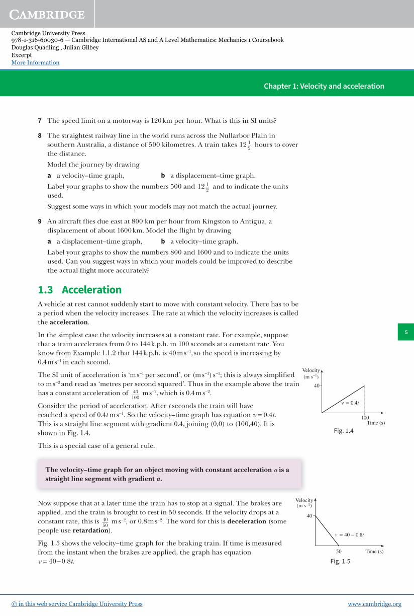
Consider the period of acceleration. After t seconds the train will have

reached a speed of 0.4t m s−1. So the velocity–time graph has equation v = 0.4t.

This is a straight line segment with gradient 0.4, joining (0,0) to (100,40). It is

shown in Fig. 1.4.

This is a special case of a general rule.

The velocity–time graph for an object moving with constant acceleration a is a

straight line segment with gradient a.

Now suppose that at a later time the train has to stop at a signal. The brakes are

applied, and the train is brought to rest in 50 seconds. If the velocity drops at a

constant rate, this is 4050

m s−2, or 0.8 m s−2. The word for this is deceleration (some

people use retardation).

Fig. 1.5 shows the velocity–time graph for the braking train. If time is measured

from the instant when the brakes are applied, the graph has equation

v = 40 − 0.8t.

Velocity

(m s–1)

Time (s)100

40

= 0.4

Fig. 1.4

Velocity(m s–1)

Time (s)50

40

= 40 − 0.8

Fig. 1.5

5



www.cambridge.org



There are two new points to notice about this graph. First, it doesn’t pass through the

origin, since at time t = 0 the train has a velocity of 40 m s−1. The velocity when t = 0 is

called the initial velocity.

Secondly, the graph has negative gradient, because the velocity is decreasing. This

means that the acceleration is negative. You can either say that the acceleration

is – 0.8 m s−2, or that the deceleration is 0.8 m s−2.

The displacement is still given by the area of the region between the velocity–time

graph and the t-axis, even though the velocity is not constant. In Fig. 1.4 this region is

a triangle with base 100 and height 40, so the area is 12

100 40 2000× ×100 = . This means

that the train covers a distance of 2000 m, or 2 km, while gaining speed.

In Fig. 1.5 the region is again a triangle, with base 50 and height 40, so the train

comes to a standstill in 1000 m, or 1 km.

A justii cation that the displacement is given by the area will be found in Section 11.3.

1.4 Equations for constant accelerationYou will often have to do calculations like those in the last section. It is worth

having algebraic formulae to solve problems about objects moving with constant

acceleration.

Fig. 1.6 shows a velocity–time graph which could apply to any problem of this type.

The initial velocity is u, and the velocity at time t is denoted by v. If the acceleration

has the constant value a, then between time 0 and time t the velocity increases by

at. It follows that, after time t,

v = u + at.

Remember that in this equation u and a are constants, but t and v can vary.

In fact, this equation is just like y = mx + c (or, for a closer comparison, y = c + mx).

The acceleration a is the gradient, like m, and the initial velocity u is the intercept,

like c. So v = u + at is just the equation of the velocity–time graph.

There is, though, one important difference. This equation only applies so long as the

constant acceleration lasts, so the graph is just part of the line.

There are no units in the equation v = u + at. You can use it with any units you like,

provided that they are consistent.

To i nd a formula for the displacement, you need to i nd the area of the shaded

region under the graph between (0,u) and (t,v) in Fig. 1.6. You can work this out in

either of two ways, illustrated in Figs. 1.7 and 1.8.

Velocity

Time

Velocity

Time

Fig. 1.7 Fig. 1.8

Velocity

Time

( , )

gradient

Fig. 1.6

6



www.cambridge.org



In Fig. 1.7 the region is shown as a trapezium, with parallel vertical sides of length u

and v, and width t. The formula for the area of a trapezium gives

s t12( )u v+u .

Fig. 1.8 shows the region split into a rectangle, whose area is ut, and a triangle with

base t and height at, whose area is 12

× t a× t . These combine to give the formula

s ut at= ut 12

2 .

EXAMPLE 1.4.1

A racing car enters the i nal straight travelling at 35 m s−1, and covers the 600 m

to the i nishing line in 12 s. Assuming constant acceleration, i nd the car’s speed

as it crosses the i nishing line.

Measuring the displacement from the start of the i nal straight, and using SI

units, you know that u = 35. You are told that when t = 12, s = 600, and you

want to know v at that time. So use the formula connecting u, t, s and v.

Substituting in the formula s t12( )u v+u ,

600 5 1212

= 12

×( )35 +35 .

This gives 35600 2

12100+ =

×=v , so v = 65.

Assuming constant acceleration, the car crosses the i nishing line at 65 m s−1.

EXAMPLE 1.4.2

A cyclist reaches the top of a slope with a speed of 1.5 m s−1, and accelerates at

2 m s−2. The slope is 22 m long. How long does she take to reach the bottom of

the slope, and how fast is she moving then?

You are given that u = 1.5 and a = 2, and want to i nd t when s = 22. The

formula which connects these four quantities is s ut at= ut 12

2 , so

displacement and time are connected by the equation

s = 1.5t + t 2.

When s = 22, t satisi es the quadratic equation t 2 + 1.5t − 22 = 0. Solving this

by the quadratic formula (see P1 Section 4.4), t =− ± − ×1 5 1 5 4 1×

2

2. .±5 1 ( )−22,

giving t = −5.5 or 4. In this model t must be positive, so t = 4. The cyclist

takes 4 seconds to reach the bottom of the slope.

To i nd how fast she is then moving, you have to calculate v when t = 4. Since

you now know u, a, t and s, you can use either of the formulae involving v.

The algebra is simpler using v = u + at, which gives

v = 1.5 + 2 × 4 = 9.5.

The cyclist’s speed at the bottom of the slope is 9.5 m s−1.

7



www.cambridge.org



Exercise 1B1 A police car accelerates from 15 m s−1 to 35 m s−1 in 5 seconds. The acceleration

is constant. Illustrate this with a velocity–time graph. Use the equation v = u + at

to calculate the acceleration. Find also the distance travelled by the car in that

time.

2 A marathon competitor running at 5 m s−1 puts on a sprint when she is 100 metres

from the i nish, and covers this distance in 16 seconds. Assuming that her

acceleration is constant, use the equation s t12( )u v+u to i nd how fast she is

running as she crosses the i nishing line.

3 A train travelling at 20 m s−1 starts to accelerate with constant acceleration. It covers

the next kilometre in 25 seconds. Use the equation s ut at= ut 12

2 to calculate

the acceleration. Find also how fast the train is moving at the end of this time.

Illustrate the motion of the train with a velocity–time graph.

How long does the train take to cover the i rst half kilometre?

4 A long-jumper takes a run of 30 metres to accelerate to a speed of 10 m s−1 from a

standing start. Find the time he takes to reach this speed, and hence calculate his

acceleration. Illustrate his run-up with a velocity–time graph.

5 Starting from rest, an aircraft accelerates to its take-off speed of 60 m s−1 in a

distance of 900 metres. Assuming constant acceleration, i nd how long the take-off

run lasts. Hence calculate the acceleration.

6 A train is travelling at 80 m s−1 when the driver applies the brakes, producing a

deceleration of 2 m s−2 for 30 seconds. How fast is the train then travelling, and

how far does it travel while the brakes are on?

7 A balloon at a height of 300 m is descending at 10 m s−1 and decelerating at a rate of

0.4 m s−2. How long will it take for the balloon to stop descending, and what will its

height be then?

1.5 More equations for constant accelerationAll the three formulae in Section 1.4 involve four of the i ve quantities u, a, t, v and s.

The i rst leaves out s, the second a and the third v. It is also useful to have formulae

which leave out t and u, and you can i nd these by combining the formulae you

already know.

To i nd a formula which omits t, rearrange the formula v = u + at to give at = v − u, so

tv u

a= . If you now substitute this in s t1

2( )u v+u , you get

sv u

a×1

2( )u v+u ,

which is 2as = (u + v)(v − u). The right side of this is (v + u)(v − u) = v 2 − u2, so that

i nally 2as = v 2 − u2, or

v 2 = u2 + 2as.

8



www.cambridge.org



The i fth formula, which omits u, is less useful than the others. Turn the formula

v = u + at round to get u = v − at. Then, substituting this in s ut at= ut 12

2 , you get

s t at( )v at−v 12

2 , which simplii es to

s vt atvt 12

2 .

For an object moving with constant acceleration a and initial velocity u, the

following equations connect the displacement s and the velocity v after a time t.

at s ut at v u as

s t s vt at

= +u = ut = +u

vt

12

12

12

2 2v

2

2

2

( )u v+u

You should learn these formulae, because you will use them frequently throughout

this mechanics course.

EXAMPLE 1.5.1

The barrel of a shotgun is 0.9 m long, and the shot emerges from the muzzle

with a speed of 240 m s−1. Find the acceleration of the shot in the barrel, and the

length of time the shot is in the barrel after i ring.

In practice the constant acceleration model is likely to be only an approximation, but it

will give some idea of the quantities involved.

The shot is initially at rest, so u = 0. You are given that v = 240 when s = 0.9,

and you want to i nd the acceleration, so use v2 = u2 + 2as.

240 0 2 0 92 20= 00 × ×a . .9

This gives a = =240

2 0× 932000

2

..

You can now use any of the other formulae to i nd the time. The simplest is

probably v = u + at, which gives 240 = 0 + 32 000t, so t = 0.0075.

Taking account of the approximations in the model and the data, you can

say that the acceleration of the shot is about 30 000 m s−2, and that the shot is

in the barrel for a little less than one-hundredth of a second.

EXAMPLE 1.5.2

The driver of a car travelling at 96 k.p.h. in mist suddenly sees a stationary bus

100 metres ahead. With the brakes full on, the car can decelerate at 4 m s−2 in

the prevailing road conditions. Can the driver stop in time?

You know from Example 1.1.2 that 96 k.p.h. is 96 518

1×

−ms , or 803

1ms− .

This suggests writing u = 803

and a = −4 in the formula v2 = u2 + 2as to i nd v

when s = 100. Notice that a is negative because the car is decelerating.

9



www.cambridge.org



When you do this, you get v 2 2

38009

2 4 100= ( )803

− 2 × =100 − . This is clearly a

ridiculous answer, since a square cannot be negative.

The reason for the absurdity is that the equation only holds so long as the

constant acceleration model applies. In fact the car stops before s reaches

the value 100, and after that it simply stays still.

To avoid this, it is better to begin by substituting only the constants in the

equation, leaving v and s as variables. The equation is then

v s2 6400

98 .

This model holds so long as v 2 0≥ . The equation gives v = 0 when s = =×

64009 8

8009

,

which is less than 100. So the driver can stop in time.

This example could be criticised because it assumes that the driver puts the brakes on

as soon as he sees the bus. In practice there would be some ‘thinking time’, perhaps

0.3 seconds, while the driver reacts. At 803

1ms− , the car would travel 8 metres in this

time, so you should add 8 metres to the distance calculated in the example. You can

see that the driver will still avoid an accident, but only just.

Exercise 1C1 Interpret each of the following in terms of the motion of a particle along a

line, and select the appropriate constant acceleration formula to i nd the answer.

The quantities u, v, s and t are all positive or zero, but a may be positive or

negative.

a u = 9, a = 4, s = 5, i nd v b u = 10, v = 14, a = 3, i nd s

c u = 17, v = 11, s = 56, i nd a d u = 14, a = −2, t = 5, i nd s

e v = 20, a = 1, t = 6, i nd s f u = 10, s = 65, t = 5, i nd a

g u = 18, v = 12, s = 210, i nd t h u = 9, a = 4, s = 35, i nd t

i u = 20, s = 110, t = 5, i nd v j s = 93 v = 42, t = 32

, i nd a

k u = 24, v = 10, a = −0.7, i nd t l s = 35, v = 12, a = 2, i nd u

m v = 27, s = 40, a = −4 12

, i nd t n a = 7, s = 100, v − u = 20, i nd u

2 A train goes into a tunnel at 20 m s−1 and emerges from it at 55 m s−1. The tunnel

is 1500 m long. Assuming constant acceleration, i nd how long the train is in the

tunnel for, and the acceleration of the train.

3 A motor-scooter moves from rest with acceleration 0.1 m s−2. Find an expression for

its speed, v m s−1, after it has gone s metres. Illustrate your answer by sketching an

(s,v) graph.

4 A cyclist riding at 5 m s−1 starts to accelerate, and 200 metres later she is riding at

7 m s−1. Find her acceleration, assumed constant.

5 A train travelling at 55 m s−1 has to reduce speed to 35 m s−1 to pass through a

junction. If the deceleration is not to exceed 0.6 m s−2, how far ahead of the

junction should the train begin to slow down?

10



www.cambridge.org

velocity and acceleration chapter 1 - assets - cambridge...

Documents