vehicular positioning using 5g and sensor fusion
TRANSCRIPT

IN DEGREE PROJECT INFORMATION AND COMMUNICATION TECHNOLOGY,SECOND CYCLE, 30 CREDITS
, STOCKHOLM SWEDEN 2019
Vehicular Positioning Using 5G and Sensor Fusion
SEYED SAMIE MOSTAFAVI
KTH ROYAL INSTITUTE OF TECHNOLOGYSCHOOL OF ELECTRICAL ENGINEERING AND COMPUTER SCIENCE


Vehicular Positioning Using5G and Sensor Fusion
SEYED SAMIE MOSTAFAVI
Master in Communication SystemsDate: November 7, 2019Supervisor: Prof. Mikael JohanssonIndustrial Supervisors: Dr. Burak Guldogan and Stefano SorrentinoExaminer: Dr. Gabor FodorSchool of Electrical Engineering and Computer ScienceHost company: Ericsson ABSwedish title: Fordonsplacering med Hjälp av 5G och Sensorfusion


iii
AbstractRecent advances in the telecommunications industry and the resulting appli-cations such as autonomous vehicles, vehicle surveillance and traffic safetyhas increased the demand for accurate and robust vehicle positioning systems.Existing Global Navigation Satellite System (GNSS) based positioning tech-niques face significant performance loss in the tunnels and urban canyons.Recent researches have shown that radio-based positioning techniques are the-oretically promising to make an accurate navigation system to fill the GNSSgaps. Fifth generation of mobile communication (5G) will utilize wide band-widths together with beamforming enabled by antenna arrays to provide higherdata rates to mobile users. These features make 5G a favorable candidate forhigh accuracy positioning. On the other hand, sensor fusion is commonly em-ployed to develop more robust and accurate navigation systems for vehicles. Inthis work, the range and angle measurements from 5G base stations are fusedwith the acceleration measurements by the means of the extended Kalman fil-ter to generate position estimates for a moving car. The accuracy of this posi-tioning system is studied with centimeter wave (cmWave) and millimeter wave(mmWave) 5G cellular networks which are set up by practical parameters. To-wards that, the positioning system is tested in a simulation-based experimentwhere a car is moving on a highway and the 5G base stations are deployedalongside of it. Based on that, a detailed analysis of the Kalman filter’s rootmean squared error (RMSE) and the 5G’s different parameters and limitingfactors such as the line of sight (LOS) blockage is carried out. Our numericalresults show that vehicles connected to 5G can benefit from this system to en-hance the robustness and accuracy of their navigation system.
Key Words:Positioning, 5G, Sensor Fusion, Beamforming, IMU, Kalman Filter

iv
SammanfattningDe senaste framstegen inom telekommunikationsindustrin och de resulteran-de applikationerna som autonoma fordon, fordonsövervakning och trafiksä-kerhet har ökat efterfrågan på exakta fordonspositioneringssystem. Existeran-de Global Navigation Satellite System (GNSS) baserade positioneringstekni-ker har en betydande prestandaförlust i tunnlar och urbana kanjoner. Forsk-ning har visat att radiobaserade positioneringstekniker har mindre distribu-tionskostnader och kan vara mer exakta än satellitbaserade navigationssystem.I den femte generation av mobilkommunikation (5G) används tekniker sommillimeterWave (mmWave) och multiple-input multiple-output (MIMO) därradio-terminaler består av stora matrisantenner och arbetar med stora band-bredder. Dessa funktioner gör 5G-system gynnsamma för positionering medhög noggrannhet. Å andra sidan har informationsfusion av Inertial Naviga-tion Systems (INS) och andra positioneringstekniker vanligen använts för attutveckla mer robusta och exakta spårningssystem. I denna studie föreslår viett INS/5G-positioneringssystem för att spåra landfordon baserat på Kalmanfiltret. Vi adresserar systempositioneringsgränserna i termer av 5G nya radio(NR) subsystem och en detaljerad analys av beroendet av rotmedelfelteradkvadratfel (RMSE) för olika systemparametrar som utförs. Systemet testas iett enkelt simuleringsbaserat experiment som består av en rak motorväg medbasstationerna placerade bredvid det. Slutligen visar våra numeriska resultatatt det föreslagna systemet är i stånd att lokalisera ett UE-monterat fordon medsub-meter lägesfel även i närvaro av hård siktlinje blockering.

Contents
Acronyms vii
1 Introduction 11.1 Background . . . . . . . . . . . . . . . . . . . . . . . . . . . 11.2 Related Works . . . . . . . . . . . . . . . . . . . . . . . . . . 31.3 Motivation and Objectives . . . . . . . . . . . . . . . . . . . 51.4 Ethics and Public Welfare . . . . . . . . . . . . . . . . . . . . 61.5 Thesis Outline . . . . . . . . . . . . . . . . . . . . . . . . . . 6
2 Background 72.1 Communication System Model . . . . . . . . . . . . . . . . . 7
2.1.1 Geometry . . . . . . . . . . . . . . . . . . . . . . . . 82.1.2 Channel Model . . . . . . . . . . . . . . . . . . . . . 92.1.3 Transmission Model . . . . . . . . . . . . . . . . . . 102.1.4 Received Signal Model . . . . . . . . . . . . . . . . . 112.1.5 LOS Blockage . . . . . . . . . . . . . . . . . . . . . 11
2.2 Cramér-Rao Lower Bounds . . . . . . . . . . . . . . . . . . . 132.3 Data Fusion Using Kalman Filter . . . . . . . . . . . . . . . . 18
2.3.1 State Prediction . . . . . . . . . . . . . . . . . . . . . 192.3.2 Measurement and Update . . . . . . . . . . . . . . . . 21
3 Methodology 223.1 Research Process . . . . . . . . . . . . . . . . . . . . . . . . 233.2 Experimental Setup . . . . . . . . . . . . . . . . . . . . . . . 243.3 Data Collection . . . . . . . . . . . . . . . . . . . . . . . . . 25
4 System Design and Implementation 264.1 Cellular Network Model Implementation . . . . . . . . . . . . 27
4.1.1 Setup . . . . . . . . . . . . . . . . . . . . . . . . . . 274.1.2 Measurement . . . . . . . . . . . . . . . . . . . . . . 30
v

vi CONTENTS
4.1.3 Error Boundary Analysis . . . . . . . . . . . . . . . . 314.2 IMU Model Implementation . . . . . . . . . . . . . . . . . . 334.3 LOS Blockage Model Implementation . . . . . . . . . . . . . 354.4 Kalman Filter Implementation . . . . . . . . . . . . . . . . . 36
4.4.1 State Prediction . . . . . . . . . . . . . . . . . . . . . 374.4.2 Update Using IMU Measurements . . . . . . . . . . . 384.4.3 Update Using Cellular Network Measurements . . . . 394.4.4 Kalman Filter Visualization and Verification . . . . . 41
4.5 Kalman Filter Tuning and Vehicle Trajectory Generation . . . 43
5 Results and Analysis 465.1 Simulation Scenario and Parameters . . . . . . . . . . . . . . 465.2 Cellular Measurements Analysis . . . . . . . . . . . . . . . . 485.3 GNSS/IMU Sensor Fusion . . . . . . . . . . . . . . . . . . . 525.4 5G/IMU Sensor Fusion . . . . . . . . . . . . . . . . . . . . . 535.5 Measurement Noise Covariance . . . . . . . . . . . . . . . . 575.6 Parametric Study . . . . . . . . . . . . . . . . . . . . . . . . 57
5.6.1 Bandwidth . . . . . . . . . . . . . . . . . . . . . . . 585.6.2 Number of Sequential Symbols . . . . . . . . . . . . 595.6.3 Number of user equipment (UE) antennas . . . . . . . 595.6.4 Number of base station (BS) antennas . . . . . . . . . 60
6 Conclusions 636.1 Limitations . . . . . . . . . . . . . . . . . . . . . . . . . . . 646.2 Future Works . . . . . . . . . . . . . . . . . . . . . . . . . . 64
Bibliography 65

Acronyms
3GPP 3rd generation partnership project5G fifth generation of mobile communication
AEB angle error boundAOA angle of arrivalAOD angle of departure
BS base station
cmWave centimeter waveCRLB Cramér-Rao lower bound
FIM Fisher information matrix
GNSS Global Navigation Satellite SystemGPS Global Positioning System
i.i.d independent and identically distributedIMU inertial measurement unitINS Inertial Navigation SystemISD inter-site distance
LOS line of sight
MIMO multiple-input-multiple-outputmmWave millimeter wave
vii

viii Acronyms
NLOS non-line-of-sightNR new radio
OFDM orthogonal frequency division multiplexing
PDF probability density functionPRB physical resource block
QoS quality of service
REB range error boundRMa rural macroRMS root mean squaredRMSE root mean squared errorRSU road side unitRTK Real-Time Kinematic
SINR signal to interference plus noise ratioSNR signal to noise ratioSPEB squared position error boundary
TOA time of arrivalTRS Tracking Reference Signal
UE user equipmentUMa urban macroUMi urban microURA uniform rectangular array
V2I vehicle to infrastructureV2V vehicle to vehicle

Chapter 1
Introduction
1.1 BackgroundDue to recent advances in the telecommunications industry, vehicles connectedto cellular networks are becoming available and more popular. Indeed, due tovital applications such as autonomous vehicles, vehicle surveillance, trafficsafety, and traffic management, network connection is going to be inseparablefrom the future vehicles’ communication systems. Through this connection,vehicles will be able to communicate with each other or with the network in-frastructure to share important data and using them accidents can be preventedand lives can be saved. Position, or in general, the kinematic state of the ve-hicle is a critical piece of information for the safety applications. High ac-curacy positioning enables Advanced Driver-Assistance Systems and makesautonomous cars able to execute safety-related maneuvers.
In general, a position is calculated by taking into account measurementsof distances or angles to some reference points whose positions are known. Ina two dimensional plane, three reference points are enough to compute a posi-tion. This positioning problem has been tackled in different schemes for vari-ous scenarios and requirements. The most widely used solution for vehicularpositioning relies on a GNSS or Global Positioning System (GPS). Conven-tional GNSS average accuracy ranges from few meters to above 20 m, limitingits application in autonomous vehicles as decimeter level accuracy is neededto stay in lane. With the fast development of the multiple-constellation GNSS,the accuracy could be improved by using differential GPS, assisted GPS, andReal-Time Kinematic (RTK) solutions. As an example, single-frequency RTKcan provide decimeter-level positioning due to better satellite visibility andspatial geometry. However, all GNSS based solutions show significant perfor-
1

2 CHAPTER 1. INTRODUCTION
mance loss in dense urban driving environments due to poor satellite coverage.RTK performance even using multiple constellations degrades in the environ-ments with frequent signal blockages and multipaths such as in urban canyonsor tunnels [1].
Another positioning technique which has been combined with GNSS is In-ertial Navigation System (INS). INS relies on inertial sensors or inertial mea-surement units (IMU) consisted of accelerometers and gyroscopes to measurelinear accelerations and vehicle angular velocities, respectively. These dataare used to calculate the trajectory of the vehicle as it moves and the vehicleposition is being calculated relative to its initial position, in a method knownas dead reckoning [2]. INS is a self-contained system and unlike GNSS, itsperformance is not degraded due to the environment. However, INS perfor-mance degrades with time due to the accumulation of measurement errors andin order to limit the errors, regular updates from another source of position-ing is necessary. In hybrid INS/GNSS positioning systems, GNSS positionestimates are used for this purpose and the INS is able to provide position-ing solution during GNSS short outages. While INS/GNSS positioning wasable to improve the accuracy and mitigate some drawbacks of the standaloneGNSS and INS, positioning errors showed that this system was not adequatefor autonomous vehicles [3].
To address theGNSS limitations, there has been important studies on radio-based positioning techniques and the 5G has not been an exception. Comparedto the existing cellular networks, 5G is going to bring huge improvements incapacity, number of connected devices, and latency. These qualities are madepossible by higher bandwidths and advanced antenna systems. In 5G, tech-nologies such as mmWave multiple-input-multiple-output (MIMO) are used,where both UE and the BS have arrays of large number of antennas, and workat a frequency in the range of 30-300 GHz with large bandwidths. Recentresearches show that these features make 5G mmWave systems favorable forhigh accuracy positioning in the order of 30 centimeters [4]. 5G signals arealso vulnerable to the blockage and in non-line-of-sight (NLOS) the position-ing performance degrades intensely. However, since the deployment cost of abase station is very much less than a navigation satellite and the accuracy isbetter, shifting from GNSS to cellular network based positioning technologiesseems promising [4].
As mentioned above, being connected to the network is going be a certainfeature of the vehicles. On the other hand, recent researches showed undeni-able advantages of 5G positioning technologies over GNSS [4]. Hence, 5Gconnected vehicles could benefit from both side if a robust, invulnerable to

CHAPTER 1. INTRODUCTION 3
blockage, and standardized network based positioning technique was avail-able.
1.2 Related WorksSharing the state, including speed, heading, and location in network connectedvehicles can be done in two different ways: the vehicle can broadcast its stateto other vehicles in a vehicle to vehicle (V2V) form or it can send its state to acellular base station or a road side unit in a vehicle to infrastructure (V2I) form.Based on these two architectures, various positioning techniques are proposedin the literature. The potential advantages of the V2I positioning over V2Vpositioning include: 1) more accurate position estimates due to fixed positionof road side units (RSU); 2) more reliability since the number of RSUs withinthe transmission range can be guaranteed; 3) important information can besent to the network from the vehicle and broadcasted to the vehicles from thetraffic control center. (e.g., events such as accidents in the area) [4].
Furthermore, main reason that 5G network is a promising candidate for po-sitioning is that it is expected to offer increased reliability, reduced latency, andhigher throughput compared to current mobile networks. Vehicular V2I posi-tioning based on IEEE 802.11p which is a vehicular communication protocolis also possible. However, its drawback is the large number of RSU installa-tion cost required for continuous communication while the use of existing 5Gcellular infrastructure for positioning will save huge amount of capital expen-diture [4]. Therefore, main focus of this thesis will be onV2I based positioningbased on 5G cellular networks.
A lot of works have been published in order to extract the benefits of thenext generation of cellular networks for positioning. At mmWave frequencies,larger bandwidths are available and they enable more accurate time of arrival(TOA) or time difference of arrival measurements. These measurements canbe used for range estimation and the ranging from at least 3 fixed nodes oranchors (in 2 dimension space) using multilateration leads to a position esti-mation [5]. Despite promising accuracy, multi-anchor might not be practicalat cellular networks where any signal from outside of the cell on the samefrequency is considered as an interference [6].
Furthermore, in mmWave frequencies the path loss is high and beamform-ing gain is required to compensate the path loss. Due to the high frequencyof mmWaves, more antennas can be packed in the same area which enablesaccurate angle of departure (AOD) and angle of arrival (AOA) estimations.Hence, the combination of AOD or AOAwith TOAmakes position estimation

4 CHAPTER 1. INTRODUCTION
theoretically possible with a single anchor. In [6], the exact and asymptotic ex-pressions for the position, orientation and velocity error bounds of uplink ordownlink localization in static, dynamic, LOS, and NLOS scenarios are de-rived. They also analyzed the effect of imperfect time synchronization on theerror bounds. In [7], the author could derive the error bounds for differentscenarios and showed that in certain conditions multipath components of thereceived signal can be considered orthogonal and can be used to increase theaccuracy of the LOS standalone position estimation. Shahmansoori, Garcia,Destino, et al. [8] also showed the potential of locating a mmWave receivereven when the LOS is blocked and compared 2 different channel estimationmethods for that purpose. As an important outcome, Abu-Shaban, Zhou, Ab-hayapala, et al. [7] derived closed-form error bound expressions of the rangeand angles for LOS scenario which used in this thesis as a basis.
Up to this point, we argued that 5G based positioning techniques can satisfyhigh accuracy and low latency requirements of autonomous driving. However,cellular systems are not designed to maintain LOS for the UE all the time. Jain,Kumar, and Panwar [9] presented a simplified model for blockage probability,frequency, and duration in mmWave cellular systems and they suggest that thedesign of mmWave networksmay sometimes be driven by blockage rather thancapacity requirements. As mentioned above, INS usage could help GNSS inthe outage periods and it might be able to compensate high errors of 5G basedpositioning systems during the outages.
For most of navigation sensor fusion systems, the fusion algorithm worksby using a Kalman filter. A Kalman filter is a bayesian filter which operatesbased on a 2 steps in a loop: at first it makes a prediction based on the processmodel; afterwards, it updates the prediction using the measurements providedby the sensors. The process model in a positioning filter predicts the positionbased on kinematic equations and the update step is based on the prior infor-mation on the uncertainty of each measurement source. The main challengein designing a Kalman filter is that the prior model of the sensors’ noise orprocess noise is incomplete. Hence, enormous works have been done in orderto address this challenge such as [10] that proposed and developed an adaptiveKalman filter for the localization of mobile robots. In their work, measure-ments are provided by sonar and odometrical sensors to update the estimatesof a robot’s position.

CHAPTER 1. INTRODUCTION 5
1.3 Motivation and ObjectivesGNSS, GPS, and their variants are not accurate and cost efficient enough forall autonomous driving environments such as urban canyons or tunnels. 5G iscurrently being standardized and due to some unique features it is a favorablecandidate for positioning. However, since the positioning techniques based on5G are going to suffer from LOS blockage, integrating 5G positioning withINS using Kalman filter is expected to make a better positioning system andits performance should be analyzed and assessed. Since there are ongoingresearches on the channel estimation algorithms which are the base for posi-tioning in 5G, the calculation of positioning accuracy will be done regardlessof any channel state estimator and the fundamental error bounds will be con-sidered.
As mentioned above, features such as large bandwidths, high frequencies(e.g. 28 GHz), and large number of antennas in 5G are the key enablers forhigh accuracy positioning. Now 5G is close to deployment and various con-figurations of it with different resource management schemes are defined. In awireless cellular network, different factors are involved in order to satisfy thequality of service (QoS) delivered to the user: bandwidth, time, UE antennasystem, BS antenna system, transmitter power, cell radius, and etc [11]. Thequestion is how each of these factors should be designed in order to make a5G/INS positioning system achieve the required accuracy.
From another point of view, Kalman filter plays an important role and itsdownsides should be taken into account. As mentioned above, Kalman filterperformance can suffer from lack of information on the measurement and pro-cess noise models. The impact of Kalman filter design parameters on the finalaccuracy should be analyzed and assessed.
Specifically, the present thesis focuses on the following objectives:
• Study and implement a 5G positioning algorithm based on the funda-mental error bounds.
• Design and implement a Kalman filter based data fusion algorithm forcombining the IMU measurements with 5G measurements.
• Study and model the impact of cellular communication LOS blockagefor the designed positioning system.
All the implementations are mathematical computer simulations and invarious cases and Monte Carlo runs are used to examine and assess the per-formance of the system.

6 CHAPTER 1. INTRODUCTION
1.4 Ethics and Public WelfareHigh accuracy positioning is the key technology that enables important appli-cations such as autonomous vehicles, vehicle surveillance, traffic safety, andtraffic management. All of these applications can help the society reduce theenergy consumption, reduce the number of deaths caused by road accidents,and make the transportation more cost efficient and less harmful for the peo-ple and the environment. However, the main challenge in the engineering hasalways been the importance of privacy. In the present thesis’ topic, the impor-tant concern is how to keep the position estimates safe and only accessible tothe UE which is localized.
1.5 Thesis OutlineThis thesis is organized as the following structure: In chapter 2, the systemmodel which consists of the communication system, the Kalman filter, and theIMU and associated background information is described. Chapter 3 explainsthe research process, the experimental setup and the proposed data collectionmethod. The design and implementation details of the positioning system isgiven in chapter 4. Each component’s model is described in detail and its keyparameters are identified. The results of the experiments are analyzed anddiscussed in chapter 5. Finally, conclusions and future work are presented inchapter 6.

Chapter 2
Background
This chapter describes the system model and associated background informa-tion that serve as a starting point for the system design and implementation inChapter 4. Specifically, the system model consists of a communication sys-tem model and appropriate channel and received signal models, which aresummarized in the following section. Then, the closed form formulas for cal-culating the Cramér-Rao lower bounds (CRLB) of cellular measurements areintroduced. Finally, the last section pf this chapter describes the sensor fusionprocess using Kalman filter.
2.1 Communication System Model
Figure 2.1: Beamforming for a vehicle mounted UE
The communication system in this project consists of only two elementsin a 5G cellular network: vehicle mounted UE and BS. They are considered
7

8 CHAPTER 2. BACKGROUND
to be equipped with antenna arrays and be able to perform beamforming al-gorithms. Beamforming is the ability to direct radio energy through the radiochannel from a transmitter toward the intended receiver in order to overcomethe unfavorable path loss. The small wavelengths of high frequencies usedin 5G facilitate large number of antennas packed in a compact form factor toenable highly directional beams. So more antennas results more directional,narrower beams and larger gains [12]. Figure 2.1 shows how beamformingworks for a vehicle mounted UE in general. In this thesis, 3D positioning forboth uplink and downlink is considered and the communication system modelis analyzed to calculate and study range error bound (REB) and angle errorbound (AEB) using multi-beam directional beamforming with arbitrary an-tenna array geometry.
2.1.1 GeometryStudying the communication system in this thesis is about analyzing a wave-form when it is sent from an uniform rectangular array (URA) antenna placedon pT = [xT, yT, zT]T (transmitter) and received in another URA antennaplaced onpR = [xR, yR, zR]T (receiver) [13]. Based on the spherical coordinate
Figure 2.2: Spherical coordinate system used in the thesis (θ > 0 and φ > 0)
system shown in Figure 2.2, the array antennas can have different orientations.In Figure 2.3, two URAs each equipped with 25 antennas and different tilt an-gles are shown. Therefore, for a transmitter or a receiver, in addition to theposition vector, we have an orientation vector in the form: oT = [θT, φT]T andoR = [θR, φR]T respectively 1.
1The subscripts T and R refer to the transmit and receive sides, respectively, regardlessof the uplink or downlink. When the notation means BS or UE, the subscripts BS and UE isused.

CHAPTER 2. BACKGROUND 9
Figure 2.3: Left: a URA with 25 antennas and the tilt angle φ0 > 0. Right: aURA with 25 antennas and the tilt angle θ0 > 0.
Since in this thesis it is assumed that the moving vehicle is on the xy-plane,the rotations outside the xy-plane are not modeled. These rotations happenwhen the vehicle goes up or down hills and its elevation changes. However,changes in φ are important when the vehicle turns left or right and the tilt angleof the URA changes.
2.1.2 Channel ModelConsidering a transceiver system equipped with NR receive antennas and NT
transmit antennas that supports elevation and azimuth beamforming, assumingthat only LOS path is present, the channel matrix can be expressed in terms oftransmit and receive array responses as [8]
H = aRBaTT ∈ CNR×NT , (2.1)
where aR and aT are the related receive and transmit unit-norm array responsevectors respectively, B is the total path gain and β is the complex gain of theLOS path without considering array antenna gains and they modeled by
B =√NTNRβ, (2.2)
β = |β|ej2πD/λ, |β| = λ
(4πD)2.31, (2.3)
where D = ||pT − pR|| is the distance between the transmitter and the re-ceiver, and |β| is representing the path loss model. The chosen model for thesignal power estimation over the distance is the free space path lossmodel. The

10 CHAPTER 2. BACKGROUND
model’s path loss exponent is calculated by [14] based on theMonte Carlo sim-ulations of the 3rd generation partnership project (3GPP) rural macro (RMa)LOS path loss model.
Assuming the LOS path, denote AOD by (θT, φT) and AOA by (θR, φR)
where the related unit-norm array response vectors are given by
aT(θT, φT) , 1√NTe−j∆
TTk(θT,φT) ∈ CNT , (2.4)
aR(θR, φR) , 1√NRe−j∆
TRk(θR,φR) ∈ CNR , (2.5)
where k(θR, φR) = 2πλ
[cosφ sin θ, sinφ sin θ, cos θ]T is the wavenumber vec-tor, λ is the wavelength,∆R , [uR,1,uR,2, ...,uR,NR ] ,uR,n , [xR,n, yR,n, zR,n]T
is a vector of Cartesian coordinates of the nth receiver element which are de-rived from pR and oR. ∆T and uT,n are defined similarly.
Considering the narrow-band array model and denoting the TOA of theLOS path by τ , the channel can be expressed as
H(t) =√NRNTβaRaH
Tδ(t− τ) ∈ CNR×NT . (2.6)
2.1.3 Transmission ModelIt is assumed that the transmitter sends a signal inNB directional beams in thespace with Ns symbols in time as
sl(t) =Ns−1∑k=0
al,kp(t− kTs), 1 ≤ l ≤ NB, (2.7)
where Ts is the symbol duration, al,k are known pilot symbols with unit energy,transmitted over the lth beam, and p(t), is a pulse with unit energy. The pilotsignal is defined as s(t) , [s1(t), s2(t), ..., sNB(t)]T with the bandwidthW andin the output of the transmitter it is multiplied by a directional beamformingmatrix defined as
F , [f1(t), f2(t), ..., fNB(t)] ∈ CNT×NB , (2.8)fl = 1√
NBaT,l(θl, φl), 1 ≤ l ≤ NB. (2.9)
In order to keep the transmitted power fixed with differentNT andNB, it can beshown that Tr(FHF) = 1 and E[s(t)sH(t)] = INB . Therefore the transmittedsignal is in the form
e(t) =√EsFs(t) ∈ CNT , (2.10)
where Es is the transmitted energy per symbol duration.

CHAPTER 2. BACKGROUND 11
2.1.4 Received Signal ModelAssuming there is only one transmitter, the received signal considering abovedefinitions can be expressed as
r(t) = H(t) ~ e(t) + n(t) ∈ CNR , (2.11)
where n(t) , [n1(t), n2(t), ..., nNR(t)]T ∈ CNR is white Gaussian zero-meannoise with power spectral density of N0. To obtain the fundamental lowerbounds regardless of the type of processes at the receiver, it is assumed thata low-noise amplifier and an ideal passband filter are attached to each receiveantenna. In order to elaborate Equation 2.13, the transmission model term andthe channel model term are replaced from Equations 2.10 and 2.6 respectivelyand the result is
r(t) =√NRNTEsβaRaH
TFs(t− τ) + n(t) ∈ CNR . (2.12)
Considering the received signal is periodic with TS and Es = PTTs, the re-ceived power without noise can be expressed as
PR = PT NTNR ||aTF||2 |β|2 (2.13)
In this research’s experiments, more than one transmitter are present in thenetwork. In this case, first, the signal of the desired transmitter (indicated withi), is affected by the beamforming and pathloss. Next, in addition to the ther-mal noise with the power N0W , the signal is added by the other transmitters’signals (indicated with j) with the total power of ΣPR,j . This interference isadded to the noise power and based on that the signal to interference plus noiseratio (SINR) at the receiver can be written as
SINR = PT,i︸︷︷︸TxiPower
×NT,iNR,i||aT,iFi||2︸ ︷︷ ︸Beamforming Gain
× |βi|2︸︷︷︸Path Loss︸ ︷︷ ︸
Received Power PR,i from BSi
× 1
N0W + ΣPR,j︸ ︷︷ ︸Noise + Interference Power
, (2.14)
where N0 = −170 dBm/Hz is the power spectral density of the noise.
2.1.5 LOS BlockageAll the assumptions in the above equations were based on the LOS availability.Since the performance of positioning techniques in LOS blocked situationsdrops significantly, no shadow fading or multi-path fading is considered in this

12 CHAPTER 2. BACKGROUND
thesis and only simple blockage is modeled. This model captures whether thecommunication between the UE and BS is possible or not. According to 3GPPtechnical report [15], assuming d2D is the distance from UE to BS in xy-plane,for different environment scenarios such as urban micro (UMi), urban macro(UMa), and RMa, the corresponding LOS probability functions are defined inthe form
PrRMaLOS =
{1 d2D ≤ 10m
exp(−d2D−10
1000
)d2D > 10m,
(2.15)
PrUMiLOS =
{1 d2D ≤ 18m18d2D
+ (1− 18d2D
) exp(−d2D
36
)d2D > 18m,
(2.16)
PrUMaLOS =
1 d2D ≤ 18m[
18d2D
+ (1− 18d2D
) exp(−d2D
36
)]× d2D > 18m,[
1 + 1.25C ′(hUT)( d2D100
)3 exp(− d2D
150
)] (2.17)
where
C ′(hUT) =
{1 hUT ≤ 13m(hUT−13
10
)1.513m < hUT ≤ 23m.
Using d2D, hUT, and above equations, the LOS probability can be calculated.However, these equations does not provide information about the duration orprobability of arrival of the blockage. In Figure 2.4, two blockage model ex-amples for a moving vehicle are shown that the probability of the blockage inboth of them is 0.5 but the duration and arrival rates are different.
The difference between these two scenarios is important for the position-ing system being analyzed in this thesis. In Figure 2.4 a, blockages are shortand frequent. In 2.4 b, blockages are long and less frequent. As mentioned be-fore, INS systems are prone to the accumulative errors. If they operate alone,after a while the error will be large. Therefore, in scenario b, using a INS/5Gpositioning system, errors will be larger than the same setup with scenario a.
In order to address this difference, two independent models in the spacedomain (xy-plane) are used for LOS blockage arrival rate and LOS blockageduration. Usually the blockage models are in the time domain but in this thesiswe assume the models are static and restricted to be in the xy-plane. It meanssome positions are in the blockage zones and others have LOS coverage. Formathematical simplicity, we assume the blockage duration is exponentiallydistributed with parameter µ which represents the expected length of a block-age event in meters. Considering X , a random variable indicating blockage

CHAPTER 2. BACKGROUND 13
(a)
(b)
Figure 2.4: Two blockage scenarios with the same 50% LOS blockage proba-bility: a) 5 short blockage events, b) 3 long blockage events.
events duration in meters, the probability mass function is in the form
P(X = χ) = µeµχ. (2.18)
For LOS blockage arrival rate the model is a Poisson distribution with param-eter λwhich is the expected number of blockage occurrences per unit distance(meter). Assuming Ψ, a random variable indicating the number of blockageoccurrences per meters, the probability mass function is in the form
P(Ψ = k) =λke−λ
k!. (2.19)
In order to generate the position steps that blockage occurs, we use the fact thatif the number of events per unit distance follows a Poisson distribution, thenthe amount of distance between events follows the exponential distribution.
2.2 Cramér-Rao Lower BoundsHaving defined the communication model, we provide CRLBs derivations forrange and angle. In estimation theory CRLB expresses a lower bound on the

14 CHAPTER 2. BACKGROUND
variance of unbiased estimators of a deterministic unknown parameter [16].More importantly, it can measure how much information about an unknownparameter exists in a modeled random variable. CRLB provides that the vari-ance of any unbiased estimator is at least as high as the inverse of the Fisherinformation.
Considering a set of deterministic parameters η = [η1, η2, η3, ..., ηp]T and
N samples given by y = [y1, y2, y3, ..., yN ] with probability mass functionf(y;η), p number of estimates will be in the form
G(y) = η = [η1, η2, η3, ..., ηp]T, (2.20)
where G is an unbiased estimator and the error co-variance matrix for thevector of estimates is given by
Cη = var(η) = E[(η − η)(η − η)T
]. (2.21)
Assuming f(y;η) satisfies the regularity condition
E
[∂lnf(y;η)
∂η
]= 0,∀η, (2.22)
where the expectation is given with respect to f . Then according to Cramér-Rao theorem, the co-variance matrix ofG satisfies
Cη ≥ J−1η , (2.23)
where J(η) is the Fisher information matrix (FIM) [16]. As the name states,FIM is a way of measuring the amount of information about the unknownparameter η that an observable random variable y carries. Assuming twonormally distributed probability density functions (PDF) of y and taking themean of the random variables as the unknown parameter, it is clear that thesharper one has more information about the unknown parameter. The mainidea behind FIM is to measure the sharpness of the PDF which determineshow accurately we can estimate η. Therefore, there are second derivatives ofthe PDF with respect to η in the FIM formulation. The FIM is given by
[Jη]i,j = −E[∂lnf(y;η)
∂ηi∂ηTj
]. (2.24)
In a special case where the model is given by
yn = µn + wn, (2.25)

CHAPTER 2. BACKGROUND 15
whereµn is dependent on the parameter vector η = [η1, η2, η3, ..., ηp]T andwn
is an unbiased white Gaussian noise process with the variance of σ2. Then,the FIM becomes [16]
[Jη]i,j =1
σ2
N−1∑n=1
∂µHn
∂ηi
∂µn∂ηj
. (2.26)
Similarly, for the continuous form of µ(t), FIM can be written as
[Jη]i,j =1
σ2
∫ T
0
<{∂µH
∂ηi
∂µ
∂ηj
}. (2.27)
To obtain the CRLB of AOD,AOA, and TOA, we define the parametervector in the form
ϕ , [θR, θT, φR, φT, τ ]T. (2.28)
Then, the corresponding FIM is structured as
Jϕ ,
JθRθR JθRθT . . . JθRτJθTθR
. . . . . ....
... . . .. . . ...
JτθR . . . . . . Jττ
, (2.29)
where due to the additive white Gaussian noise and according to Equation2.27, FIM can be derived as
[Jϕ]i,j =1
N0
∫ NsTs
0
<{∂µH
ϕ(t)
∂ϕi
∂µϕ(t)
∂ϕj
}. (2.30)
And the noiseless part of received signal in Equation 2.12, µϕ(t) is expressedas
µϕ(t) ,√NRNTEsβaRaH
TFs(t− τ). (2.31)
By replacingEs = PTTs and Ts ≈ 1/W , we define γ , NRNTNsPT/(N0W+
ΣPR,j) and assuming the following notations [7]
KR , diag(
∂
∂θR∆T
Rk(θR, φR)
), (2.32a)
KT , diag(
∂
∂θT∆T
Tk(θT, φT)
), (2.32b)
PR , diag(
∂
∂φR∆T
Rk(θR, φR)
), (2.32c)
PT , diag(
∂
∂φT∆T
Tk(θT, φT)
), (2.32d)

16 CHAPTER 2. BACKGROUND
and according to [7], Jϕ, the FIM of the AOA,AOD, and TOA is derived asfollows
Jϕ = γ|β|2
RθG 0 Xθ,φG 0 0
0 LθG
0Yθ,φG
0
Xθ,φG 0 RθG 0 0
0Yθ,φG
0 LθG
0
0 0 0 0 4π2GW 2
, (2.33)
in which
Rθ , aHRK2
RaR, Lθ , GTθ − |Vθ|2,Rφ , aH
RP2RaR, Lφ , GTφ − |Vφ|2,
Vθ , aHTKTFFHaT, Tθ , aH
TKTFFHKTaT,
Vφ , aHT PTFFHaT, Tφ , aH
T PTFFHPTaT,
G , aHTFFHaT, Yθ,φ , GY ′θ,φ −<{VφV ∗θ },
Xθ,φ , aHRKRPRaR, Y ′θ,φ , <{aH
T PTFFHKTaT}.
After inverting the FIM matrix Jϕ, the the CRLBs of the channel paramtersare given by
CRLB(θR) =1
γ|β|2G(Rθ −
X2θ,φ
Rφ
) , (2.34a)
CRLB(φR) =1
γ|β|2G(Rφ −
X2θ,φ
Rθ
) , (2.34b)
CRLB(θT) =G
γ|β|2(Lθ −
Y 2θ,φ
Lφ
) , (2.34c)
CRLB(φT) =G
γ|β|2(Lφ −
Y 2θ,φ
Lθ
) , (2.34d)
CRLB(τ) =1
(4π2W 2)(γ|β|2G). (2.34e)
Based on the CRLB closed form formulas, AOA, AOD, and ranging errorbounds can be obtained. The CRLBs of the angles consist of 2 components:First, the SINR component γ|β|2G for the receiver angles, andG/γ|β|2 for thetransmitter angles. Second, other spatial information in the parentheses. TheCRLB of τ is dependent on the SINR and bandwidth. It should be noted that

CHAPTER 2. BACKGROUND 17
in the SINR component, NS is involved. However, for reporting the SINR ofthe signal, it is assumed that the orthogonal frequency division multiplexing(OFDM) symbols are separately received and the SINR is calculated regard-less of NS.
As shown in Figure 2.5, it should be noted that the BS’s position and ori-entation are always fixed and known, hence, only angle measurements relatedto the BS are useful. In the downlink case, when BS is sending out pilot sig-nals, θT, φT, and τ should be calculated. In the uplink case, when the UE istransmitting pilot signals, θR, φR, and τ should be calculated. Considering cthe speed of light, AEBs and REBs in uplink and downlink are obtained andshown in Table 2.1.
Figure 2.5: Resolvable unknowns in downlink vs uplink (the same for θ)
Table 2.1: Error Bounds in Uplink or Downlink Mode
Uplink Downlink
AEB√
CRLB(φR),√
CRLB(θR)√CRLB(φT),
√CRLB(θT)
REB√CRLB(τ)× c
√CRLB(τ)× c

18 CHAPTER 2. BACKGROUND
2.3 Data Fusion Using Kalman FilterA Kalman filter [17] is an algorithm that can make an educated guess aboutwhat the system is going to do next where there are uncertain informationabout that dynamic system. From a theoretical aspect, the Kalman filter isan algorithm permitting exact inference in a linear dynamical system, whichis a Bayesian model where all latent and observed variables have a Gaussiandistribution (usually a multivariate Gaussian distribution). The Kalman filteris typically derived using vector algebra as a minimummean squared estimator[18].
Kalman filter can combine different measurements and relate them withthe state of the system. As shown in Figure 2.6, first, the Kalman filter makesa prediction on the next time step state based on the process model; then itcombines the received information with the prediction result to calculate thefinal estimate. The combination process is done by merging the Gaussian dis-tributions as shown in step 3. Kalman gain is also calculated in step 3 andbasically it indicates how much it needs to change the estimate.
Figure 2.6: How Kalman filter works in 3 steps.
Assume xk is a known state vector of a process at time step k and it isdesired to estimate the state vector at the next time step xk+1. If the system is

CHAPTER 2. BACKGROUND 19
linear and stationary, the state at time step k+1 can be written as [19]
xk+1 = Fxk + wk, (2.35)
where F is the noiseless state transition matrix of the process from k to k + 1
and is assumed stationary over time and wk ∼ N (w; 0,Q) is the white Gaus-sian process noise whereQ is the process noise covariance matrix. The overallobjective is to estimate xk. Assuming xk|k is the updated estimate, the dif-ference between xk|k and xk is termed the error and the mean squared errorfunction is in the form
MSE = E[f(ek)] = E[(xk − xk|k)
2], (2.36)
which may be expanded to give
Pk = E[ekeTk] = E
[(xk − xk|k)(xk − xk|k)
T] , (2.37)
where Pk is the covariance matrix of the estimate vector and it always accom-panies the estimate vector at each step.
Observations on the state vector can be modelled in the form
zk = Hxk + vk, (2.38)
where zk is the actual measurement of x at time step k, H is the noiseless con-nection between the state vector and the measurement vector, and is assumedstationary over time; vk is the associated measurement error. It is assumed tobe a white noise process with a known and stationary over time covariance R
and has zero cross-correlation with the process noise.
2.3.1 State PredictionIn the prediction step, Kalman filter calculates the predicted state xk|k−1 and itsprior covariance Pk|k−1 based on xk−1|k−1 (previous state estimate), its errorcovariancePk−1|k−1, and the prior knowledge about the system: F andQ. Theprediction equations are given by [19]
xk|k−1 = Fxk−1|k−1, (2.39)Pk|k−1 = FPk−1|k−1F
T + Q. (2.40)
The process being analyzed is the constant acceleration motion of a vehicle in2D xy-plane with the state vector in the form
xk = [xk yk xk yk xk yk]T, (2.41)

20 CHAPTER 2. BACKGROUND
where xk and yk are velocity and xk and yk are acceleration.Many process models could be chose for a land vehicle dynamics and each
would be a different implementation of Kalman filter. However, in this thesis,the state model chosen is aWiener process acceleration model. It is also calledthe nearly-constant acceleration model and is a widely used basic model whichgives a good compromise between complexity and performance [20]. Thestate transition matrix of a constant acceleration model is defined as
F =
I2 TfI2T 2f2
I202 I2 TfI202 02 I2
, (2.42)
where Tf is the sampling interval, In and 0n denote n × n identity and zeromatrices respectively. Wiener process model has two variations, first one isthe Wiener-sequence acceleration model which assumes the acceleration in-crement is an independent white noise process. The second one is called thewhite noise jerk model which assumes that the acceleration derivative ...xk isan independent white noise process. In this thesis we use the white noise jerkmodel and according to that, the process noise covariance matrix is in the form
Q = Sq
T 5f
20I2
T 4f8
I2T 3f6
I2
T 4f8
I2T 3f3
I2T 2f2
I2
T 3f6
I2T 2f2
I2 TfI2
, (2.43)
where Sq is the process noise intensity scalar and actually it is the power spec-tral density of the presumed acceleration derivative white noise process [21].In order to start the simulation, initial state x0 should be set based on Equation2.37 in the form
x0 = [x0 y0 x0 y0 x0 y0]T . (2.44)
The initial error co-variance matrixP0 is also should be defined and the diago-nal elements are the variances of the state variables in that. The off-diagonal el-ements indicate the correlations between the (errors/uncertainties in) the statevariables and they are usually zero. P0 is in the form
P0 =
σx02 0 0 0 0 0
0 σy02 0 0 0 0
0 0 σx02 0 0 0
0 0 0 σy02 0 0
0 0 0 0 σx02 0
0 0 0 0 0 σy02
. (2.45)

CHAPTER 2. BACKGROUND 21
2.3.2 Measurement and UpdateIn the update step, when the new measurement zk is obtained, Kalman filtercombines it with the predicted state xk|k−1 to create the updated estimate xk|kand update state covariance matrix Pk|k in the form
xk|k = xk|k−1 +Kk(zk −Hxk|k−1), (2.46)Pk|k = (I−KkH)Pk|k−1, (2.47)
where Kk is Kalman gain and it is given by
Kk = Pk|k−1HT(HPk|k−1H
T + R)−1. (2.48)
This step consists of pulling inmeasurements, merging Gaussian distributions,calculating Kalman gain, and updating the prediction. If there are more thanone sensors, this update step repeats sequentially number of sensors times. Im-portant factors in combining a measurement with a prediction are their noisecovariances: Pk|k−1 and R. Considering step 3 of Figure 2.6, the red curverepresents the prediction noise covariance and it is wide, which means theKalman prediction is not accurate, and the green curve represents the mea-surement noise covariance and it is thin, which means the measurement isaccurate. Therefore, the purple curve which represents the updated estimate’snoise covariance is closer to the green curve (Kalman gain is large).
Another challenge for a Kalman filter is that if the relation between xkand zk is non-linear, then to derive H, new formulas should be used. In thiscase, the non-linear function which connects xk to zk is defined in the formz = H(x). Then, according to extended Kalman filter formulations, Hk, theJacobian of the non-linear function is taken as
Hk =∂H(x)
∂x
∣∣∣∣xk|k−1
, (2.49)
where xk|k−1 is the predicted Kalman filter estimate. This formula makes alinear approximation on H around xk|k−1 and the result matrix is different foreach time step k.

Chapter 3
Methodology
The method used in this thesis to analyze the positioning system is basicallyempirical. The target system is implemented in a computer simulation envi-ronment and different experiment scenarios are defined and important factorsare modeled to emulate the real case. In this quantitative approach, the datacollection method is based on the numerous simulated experiments.
Due to the large number of hypothetically effective factors and scenarios,a comprehensive case study is conducted on a simple example problem. Asshown in Figure 3.1, the example scenario consists of a vehicle moving on ahighway and 5G network base stations deployed alongside the highway. Onthe vehicle, a 5G user terminal and an IMU is mounted and and the task is tolocalize the vehicle by mans of 5G network and IMU sensors.
Figure 3.1: The example scenario consists of a car moving on a highway and5G network base stations deployed alongside the highway.
22

CHAPTER 3. METHODOLOGY 23
Considering the utilized methods, it should be noted that this thesis aimsto find the fundamental, theoretical performance of a positioning system andit is still far from a reliable practical implementation. However, it has beentried to model most of the factors and to design the simulation environment ina realistic way.
3.1 Research ProcessThe research process of this thesis started with problem definition and the fo-cus of the research was put on the fundamental behaviour of the proposed po-sitioning system. Hence, this research can be a useful resource for other fellowresearchers. Fundamental in this project means close to the theory and inde-pendent of practical implementation limits. As mentioned in the first chapter,the problem is to study the performance of a positioning system based on 5Gcellular network and IMU data fusion.
Afterwards, the search for models, mathematical tools, and signal process-ing tools was started. For 5G cellular positioning modelling the studies in [7]was chosen due to their comprehensive and well organized work. They calcu-lated the closed form formulas for range and angle estimation in multi-antennasystems which was a great fundamental for this thesis purpose. There are var-ious stochastic filtering and data fusion algorithms available, however, due toits widely usage and simplicity, we intentionally preferred Kalman filter.
After studying the literature and finding the required tools and models,terms and concepts were defined clearly and the theoretical background wascomplete. Then the implementation of the positioning system started. Duringthe implementation of each component, the verification and evaluation of itwas a major concern and was done for all of the blocks. Moreover, finding andorganizing the impactive parameters was part of the implementation process.It should be noted that all of the system is designed and implemented in MAT-LAB. MATLAB is a numerical computing environment and a programminglanguage that most of the researchers in this field take use of it [22].
An important part of our research is designing the experiment. Eventually,the simple experiment based on the highway problem designed and all the in-dependent and dependent variables were defined and selected. Since so manyfactors were involved, various profiles and presets were defined and the systemtests were based on these predefined profiles.

24 CHAPTER 3. METHODOLOGY
3.2 Experimental SetupAll of the simulations and experiments are run in the MATLAB R2019a soft-ware. The developed code is object-oriented and customizable to enable fellowresearchers use it for more complex models or scenarios. Each component ofthe positioning system is an object in MATLAB code and during the initial-ization the parameters should be set. The car movements and trajectories aregenerated by the MATLAB automated driving toolbox [23].
Figure 3.2: Experiment setup consists of a moving car on a predefined trajec-tory and 3 base stations.
A detailed description of the experiment setup is shown in Figure 3.2. Thesetup is consisted of an arbitrary number of base stations with the distancedBS-BS from each other and the distance dBS-HW from the highway. Each basestation’s array antenna is placed in zBS height from the xy-plane and facedtoward the highway with no tilt.
In the highway there is a predefined trajectory and a car with an arrayantenna mounted along the length of it. The experiment starts from t = 1
when the car is in the initial position with a tilt of φ0. Then the car movesto the next state where it has a new position and tilt angle. For each timestep a new position estimate is generated by the positioning system and theseestimates are saved for later process. The trajectory contains NSIM samplesand the experiment continues until k = NSIM.

CHAPTER 3. METHODOLOGY 25
3.3 Data Collection
Figure 3.3: Data collection from an experiment. Red stars depict positioningsystem estimates.
As shown in Figure 3.3, in the single-run scenario, when the experimentbegins, the car connects to the positioning system and it generates positionestimates for each time step. Eventually the trajectory is finished and we have avector of position estimates for each time step. Using the initial true positionsin the trajectory, the error vector with the size NSIM can be derived and theRMSE of its samples can be calculated to give us a number representing theaccuracy.
In the multiple-run scenario, which is a Monte Carlo method, NMC exper-iments are run and in the end we have NMC × NSIM error values. Then wecalculate the RMSE of each time step to obtain an error vector with the sizeNSIM. Finally depending on the experiment, the average of this error vector orthe average of some parts of it can form the result.

Chapter 4
System Design and Implemen-tation
Figure 4.1: Implemented system architecture and data flow graph
In this chapter, the design and implementation of the proposed position-ing system is described. Figure 4.1 shows an abstract structure of the systemconsisted various separated components: cellular networkmodel, IMUmodel,Kalman filter, blockage model, and the vehicle mounter UE. Based on thesecomponents, the implementation work behind this thesis can be divided into5 parts.
26

CHAPTER 4. SYSTEM DESIGN AND IMPLEMENTATION 27
1. Implementing a simple 5G cellular network model with ranging and an-gle measurement capabilities.
2. Implementing an IMU model.
3. Modelling and implementation of the LOS blockage.
4. Implementing a 5G/IMU data fusion algorithm based on the Kalmanfilter.
5. Generating vehicle movement trajectories for the experiments.
Each item is described and elaborated in the coming sections respectively.However, there were some common challenges among them. The main chal-lenge was picking the key independent parameters, considering two concerns:First: Which parameters are challenging the performance of the system morethan the others. Second: Are the chosen independent parameters meaningfulin the industry? If not, then find and use a new one. Therefore, for each modelthe selected parameters are described and at the end of each chapters theseparameters are summarized in a table.
4.1 Cellular Network Model ImplementationThe cellular network model is an important component of the positioning sys-tem and the core functionality of it is the calculation of angle and range mea-surements’ error bounds based on equations in (2.34). However, implementa-tion details for a complete practical model are still required to be mentioned.These new elaborations are divided into two sections: Setup and Measure-ment.
4.1.1 SetupRecalling the closed-form formulas obtained in the background chapter, thecellular network has some parameters for configuration. In this section allof these parameters are mentioned and some of them revised. The model isconsisted of several base stations and for each of them (ith BS) the positionpBS,i = [xBS,i, yBS,i, zBS,i], orientation oBS,i = [φBS,i, θBS,i] can be set. The radiomeasurements are obtained from the NB transmitted beams from the squaredarray antennas at the base station withNT elements, with the carrier frequencyFc and the bandwidth ofW , transmitting power PT = ES/TS. The beams canbe sent in NS sequential symbols to enhance the measurements’ quality at the

28 CHAPTER 4. SYSTEM DESIGN AND IMPLEMENTATION
receiver (UE) with NR antennas. It is assumed that the radio communicationis only on the downlink, hence, from this point, the subscripts BS and UE referto T and R respectively. These parameters should be set during the setup phaseand they are assumed not to be changed over time.
In the receiver and transmitter array antenna, the antenna elements areplacedwith the distance d = λc/2 from each other, hence, the antenna is biggerwhen it is designed for a lower frequency. Moreover, the number of transmittedbeams are set to be on the maximum which meansNB = NT. The direction ofthese beams are uniformly distributed in the half sphere where the transmittingantenna is faced. In Figure 4.2 the beamforming gain GBF = NTNR||aTF||2for 2 different antenna setup is shown in polar plots.
(a) NBS = 64 (b) NBS = 256
Figure 4.2: The beamforming gain of the communication between a BS withNBS = 64 or 256 and a UE with NUE = 4. The UE is placed 20 m lower thanthe BS. The green line shows how the BS antenna is placed.
Figure 4.2 shows 2 important points: First, increasing the number of an-tennas does not necessarily increase the gain of each beam. It increases thenumber of beams and they become narrower. However, since NB = NT, thenumber of beams become larger and the energy is divided uniformly betweenmore beams. Hence, the gain of each beam does not change. Second, in theangles between 0 to 30 deg and 150 to 180 deg, since the distance between theantenna seems smaller, beams become undetectable for the receiver. There-fore, the UE experiences a relatively large gain which is the accumulated gainof the merged beams. In these tilted angles, the spatial information (anglemeasurement accuracy regardless of the SINR) becomes smaller too.

CHAPTER 4. SYSTEM DESIGN AND IMPLEMENTATION 29
As mentioned above, various parameters are engaged in the calculationof CRLBs. Since the objective of this thesis is to study a system based on5G, these parameters should be chosen in a way to be matched with the 5Gnew radio (NR) configurations. OFDM technique is widely used in wirelesscommunication protocols and 5G is not an exception. Using this technique,in the 5G NRs, the waveform carrying the information is a combination ofresource blocks over time and frequency, as shown in Figure 4.3 [24].
Figure 4.3: OFDM radio resource allocation scheme
An example of resource allocation in an OFDM system is shown in Figure4.3, where the number of assigned OFDM subcarriers for this waveform is 4.This means that the total bandwidth utilized for this user is 4 ×WSC, where;WSC = 1/Ts is the OFDM subcarrier spacing. This example also shows thatthe user has 6 OFDM symbols and that isNS. In 5G numerology, 12 subcarri-ers form a physical resource block (PRB) and 14 OFDM symbols form a slot[25]. It should be noted that different subcarrier spacings are defined in 5GNR. For example, in mmWave band, due to more available bandwidth, largersubcarrier spacing is defined. However, the pre-defined standard pilot signalsuse the same number of PRBs but with more bandwidth. Hence, in this thesis,the number of physical resource blocks is used instead ofW as a key param-eter to be matched with the concepts in 5G NR configurations. Therefore, thebandwidth is given by
W = NPRB ×WSC × 12, (4.1)
where NSC is the number of assigned subcarriers.

30 CHAPTER 4. SYSTEM DESIGN AND IMPLEMENTATION
Table 4.1: Summarizes the cellular network parameters.
Description NotationCarrier Frequency FcTransmitter Power PT
Subcarrier Spacing WSC
Number of Physical Resource Blocks NPRB
Number of Sequential Symbols NS
Number of UE Antennas NUE
Number of BS Antennas NBS
Cellular Measurement Rate rCel
4.1.2 MeasurementAfter the model is set up, the network model can generate the measurementsby knowing the true position and orientation of the UE. The detailed processin explained in 4 steps:
• First, the true positionpUE,k = [xUE,k, yUE,k, zUE,k] and orientationoUE,k =
[φUE,k, θUE,k] of the UE at time step k is given to the network model.
• Second, the closest BS is found and marked as the connected BS. Itsposition and orientation are known in the form pBS = [xBS, yBS, zBS]
and oBS = [φBS, θBS].
• Third, The received signal power from the connected BS, PR,i is calcu-lated. Moreover, the interference power is obtained by calculating thetotal received power Σ
j 6=iPR,j from all other BSs.
• Finally, using the CRLBs, the measurements are generated in the formzCEL,k = [rk αk]
T where αk is the angle estimation result and rk is theranging result as shown in Figure 4.4. In addition to the measurements,the connected base station position and the SINR of the connection isreported.
The error boundaries are studied in Section 2.2 and by the means of Equa-tions 2.34 and 2.1, the standard deviation of the error in angle measurementand ranging for each and every point in xy-plane is calculated. However, theerror bounds alone are not sufficient for a model and noisy angle and rangesamples are needed. In order to generate samples, as shown in Figure 4.5, an

CHAPTER 4. SYSTEM DESIGN AND IMPLEMENTATION 31
Figure 4.4: Cellular model range rk and angle αk measurement.
ideal estimator is considered where white Gaussian noise samples are addedto the true angle and true range values to generate the noisy samples in theform
rk = ζ +√
(xUE,k − xBS,c)2 + (yUE,k − yBS,c)2, (4.2)
αk = ν + arctan(yUE,k−yBS,cxUE,k−xBS,c
), (4.3)
where ζ ∼ N (0, σ2ζ ) and ν ∼ N (0, σ2
ν) are white Gaussian samples with thestandard deviations given by
σζ = (√CRLB(τ)× c). sin θ, (4.4)
σν =√
CRLB(φ), (4.5)
where CRLBs are in Equations 2.34, and calculated using the setup parametersand the position and orientation of the UE. Multiplication of sin θ is necessarybecause the CRLB is in 3D space and the σ is needed to be used in the Kalmanfilter which is in 2D space. The noiseless terms of Equations 4.2 and 4.3 aretrue range and true angle of the UE from the connected BS respectively.
4.1.3 Error Boundary AnalysisNow the communication model is complete and for each point in xy-planethere are range and angle error boundaries. For relatively small angle errors,squared position error boundary (SPEB) can be derived by [7]
SPEB = ||pBS − pUE,k||2 sin2(θ) CRLB(φ) + c2 CRLB(τ). (4.6)
Based on this equation, it is possible to analyze the performance of the devel-oped cellular model using colorful 2D plots to show howmuch is the accuracy

32 CHAPTER 4. SYSTEM DESIGN AND IMPLEMENTATION
Figure 4.5: Noisy sample generation procedure for angle and range.
of the cellular positioning on each point in the highway in front of the base sta-tions.
Figure 4.6 shows an example of boundary analysis using the SPEB formulausing (4.6). In this system, the base stations are 30m far from the highway, in-stalled in 20m of height in the downlink mode. Transmitter power is 1 dbm,only 4 antennas are available on the UE, and the total used bandwidth is 125MHz. In Figure 4.6a, 16 sequential symbols in every 10 milliseconds are usedfor the positioning with 100 BS antennas, while in Figure 4.6b, only 4 se-quential symbols used and in Figure 4.6c 16 sequential symbols with 25 BSantennas are used. As the color-bar shows, the error boundary in Figure 4.6ais much lower than the others and it is due to the larger number of sequentialsymbols and transmitter antennas. Non-uniformity of the error boundaries andhaving lobes even in the same distance from the BS is because of the narrowbeams sent from the BS to different directions. As mentioned earlier, morenumber of antennas results narrower beams and higher antenna gain. In Fig-ure 4.6c it is shown that with smaller number of antennas the beams get widerand hence the error boundaries get closer to a uniform pattern.

CHAPTER 4. SYSTEM DESIGN AND IMPLEMENTATION 33
(a) NS = 16, NBS = 100 (b) NS = 4, NBS = 100
(c) NS = 16, NBS = 25
Figure 4.6: Position error boundary analysis of 3 different deployed cellularmodels. Color-bar shows error in meters.
4.2 IMU Model ImplementationAn important parameter for any sensor is the noise density. Noise density in-dicates how much noise the samples have regardless of the sampling rate. Themodel developed for the IMU is able to generate noise based on this parame-ter. AssumingWs is the sampling rate bandwidth, calculation of the root meansquared (RMS) noise based on noise density is in the form [26]
NoiseRMS = Nd ×√Ws × 1.6, (4.7)
where Nd is the noise density of the sensor.The noisy sample generation process running for IMUmeasurements is the
same as cellular measurements generation process. Assuming xk and yk aretrue acceleration values of the vehicle, the samples generated in the IMU arewhite Gaussian noise added acceleration measurements in the form zIMU,k =

34 CHAPTER 4. SYSTEM DESIGN AND IMPLEMENTATION
[ax,k ay,k]T given by
ax,k = υ + xk, (4.8)ay,k = ω + yk, (4.9)
where ax,k and ay,k are the measured accelerations on x and y respectivelyadded by a constant bias and quantized by a specific resolution, according toEquation 4.7, υ ∼ N (0, σ2
υ) and ω ∼ N (0, σ2ω) are white Gaussian samples
with the standard deviations given by
συ = Nd√2
√1.6 rIMU/2, (4.10)
σω = Nd√2
√1.6 rIMU/2, (4.11)
where rIMU is the IMUmeasurement rate. All of the model key parameters arementioned in Table 4.2.
In order to verify the accuracy and the rate of measurements, a real Boschbmi055 IMU chip with the noise density of 150 µg/
√Hz (micro g per root
Hertz) was used, where g is the gravitational acceleration [27]. The calculatednoise density from 5k samples of Bosch sensor was 171 µg/
√Hz, a bit higher
than datasheet value due to temprature or supply voltage variations; whilethe noise density calculated from 5k samples of our model was 155 µg/
√Hz
which shows the model works as expected. Histograms of the samples for bothsources are shown in Figure 4.7.
Figure 4.7: Histogram of samples acquired from Bosch sensor (left) and ac-quired from the model (right). The gap between the bars shows the resolutionlimit is applied.
According to the Bosch bmi055 IMU chip datasheet and assuming thatthe constant bias of the sensor can be resolved using a filter, IMU parameterswhich are set for all of the the experiments are summarized in Table 4.2.

CHAPTER 4. SYSTEM DESIGN AND IMPLEMENTATION 35
Table 4.2: IMU Model Key Parameters
Description Notation ValueSensor Noise Density Nd 150 µg/
√Hz
Sensor Constant Bias C 0mgSensor Resolution Re 0.98mgIMU Measurement Rate rIMU 100 Hz
4.3 LOS Blockage Model ImplementationIn Section 2.1.5, we studied the theory behind the model of blockage for mov-ing vehicles. It is mentioned that 3 key parameters play a role in the model:LOS probability PrLOS, blockage average distance µ, and average number ofblockage events per meter λ. They are assumed to be in the space domaininstead of time and considering the example problem which is going to be an-alyzed and shown in Figure 3.1, it can be implemented in only one dimension.The overall movement of the car is towards one axis (assuming x) in a highwayand blockage arrival and duration is defined on this axis only. Then, the widthof the blockage area is set to be the width of the highway where the movementof the car is limited in. In Figure 4.8, an example is shown where the LOSblocked areas are in yellow.
Figure 4.8: A sample example of LOS blockage pattern, where the parametersare set separately. Blocked areas are in yellow. Blockage events per meterλ = 0.04 , the average blockage durationµ = 20m, LOS blockage probability:80%
In the experiments of this research, it is assumed that the base stations areclose to the highway (dBS−HW = 20 m) and since there are no standardizedLOS Blockage model for the highway scenario yet, we used the 3GPP RMamodel to calculate PrLOS using Equation 2.15.
For generating the blockage pattern, first we calculate PrLOS(d2D(x))whered2D(x) is the distance between the UE and the BS on xy−plane for each pointof the highway indicated by x. Then, it is assumed that λBlockage = 0.1 m−1

36 CHAPTER 4. SYSTEM DESIGN AND IMPLEMENTATION
and µ(x) can be derived from the equation: PrLOS(x) = 1 − λ × µ(x). Forexample in Figure 4.9, the calculated µ for the highway scenario in which a5G base station provides cellular coverage is shown. As expected, when d2Dincreases, the average length of the LOS blockage events increases.
(a) Blockage pattern
(b) LOS Blockage length (c) LOS Blockage probability
Figure 4.9: A sample example of blockage pattern of the highway scenario inwhich a 5G base station provides cellular coverage. First, the blockage prob-ability is calculated for each point (c). Second, the length of events are calcu-lated (b). Finally, the blockage pattern is generated and shown in (a). Blockedareas are in yellow and the BS is indicated with the blue circle.
4.4 Kalman Filter ImplementationThe core block of the positioning system is a Kalman filter which is imple-mented and designed based on the Kalman filter equations discussed in Sec-tion 2.3. Shown in Figure 4.10, Kalman filter starts by predicting the nextstate using the previous state and then updates this predicted state using themeasurements. There are two sources of measurement: 5G cellular networkand IMU. They may have different update rates and Kalman should be im-plemented in a flexible way that any sensor with any measurement rate canbe attached to it. Therefore, before applying the measurements it is checked(blue blocks shown in Figure 4.10) by the measurement rate, whether an up-

CHAPTER 4. SYSTEM DESIGN AND IMPLEMENTATION 37
date should be executed using IMUor cellular at time step k or not. For cellularupdate, in addition to the rate, blockage status is checked, hence if it is not theright time for cellular update or the connection is blocked, the update does nothappen.
Figure 4.10: Kalman filter implementation detailed block diagram.
4.4.1 State PredictionIn the state prediction step, Kalman filter generates the state xk|k−1 and thenoise covariance Pk|k−1. The predicted noise covariance is important since itis compared to the measurements’ noise covariance to determine how muchthe measurements should take part in the update stage. Predicted state noisecovariance is generated from process noise covariance and process noise co-variance Q is a prior knowledge about the process and should be set duringthe Kalman setup phase. It indicates how much the actual state might differfrom the process model defined.

38 CHAPTER 4. SYSTEM DESIGN AND IMPLEMENTATION
For example in our case, when a Kalman filter tracks a car, and the pro-cess model is defined as a constant acceleration model, the car’s movementmight not be always constant acceleration. When it turns or suddenly brakes,the movement is out of the constant acceleration scope. The variance of theacceleration process noise defined in Equation 2.43, σ2
Q, captures randomnessof the unknown acceleration values. From the definition it is clear that in amovement scenario when the car brakes harshly or turns sharply this param-eter is high. However, it has no relation with the constant speed of the car orthe constant acceleration movements either, only variable acceleration move-ments are important and that might degrade the performance of the Kalmanfilter. Moreover, with the presence of an IMU and acceleration measurementsfor every time step, it can be compensated to a certain level.
Two remaining pieces of puzzle are measurement noise covariance matrixR and the connectionmatrixH for IMU and cellular update. It is mentioned inSection 2.3.2 that how impactive they are on the performance of the Kalmanfilter. R matrix expresses how accurate the measurements are and they areconsidered prior knowledge about the measurement units. For IMUs, sincethe information about the acceleration measurements’ noise is available in thedatasheets the noise covariance matrix elements can be calculated from them.However, for cellular network measurements parameters such as the band-width, the distance from UE to BS, UE antenna tilt angles, and etc changethe accuracy and it is more complex. In the next two sections, the integrationof IMU and cellular measurements are discussed.
4.4.2 Update Using IMU MeasurementsDue to the linearity of the model, update stage of the IMU is simple and ob-servations at the time step k are in the form zIMU,k = [ax,k ay,k]
T and the con-nection between the state vector and the measurement matrix which is definedas HIMU is in the form
HIMU =
[0 0 0 0 1 00 0 0 0 0 1
]. (4.12)
Themeasurement noise covariance is a prior information about a sensor. Sincethe noise figure of IMU does not change with any of the parameters presentedin this thesis, we set the measurement noise covariance RIMU based on Equa-tion 4.10 and 4.11 in the form
RIMU =
[σ2υ 0
0 σ2ω
]. (4.13)

CHAPTER 4. SYSTEM DESIGN AND IMPLEMENTATION 39
The rest of the update calculations are based on equations presented in Section2.3.2.
4.4.3 Update Using Cellular Network MeasurementsThe case for the cellular measurement is different. The observations from thecellular positioning are in the form zCEL,k = [rk αk]
T consisting of range andangle data which cannot be transformed to a state vector consisting of x andy coordinates easily. Assuming the function hr(xk) can calculate the range rfrom the state vector xk and hα(xk) can calculate the angle α from the statevector, they are in the form
rk = hr(xk) =√
(xk − xBS)2 + (yk − yBS)2, (4.14)
αk = hα(xk) = arctan(yk−yBSxk−xBS
), (4.15)
where (xBS, yBS) is the position of the connected BS and the origin of the rangeand angle calculated based on TOA and AOD in the downlink mode.
As equations show, the cellular measurements models are non-linear andfor the calculation of Hk the extended Kalman filter formulation should beused and recalling from Section 2.49, it is formulated in the form [16]
Hk =∂H(x)
∂x
∣∣∣∣xk|k−1
, (4.16)
where xk|k−1 is the predicted state and H(x) is defined by
H(x) = [hr(x) hα(x)]T. (4.17)
Using the formula on the hr(xk) and hα(xk) results in
HCEL,k =
xk|k−1−xBSrk|k−1
yk|k−1−yBSrk|k−1
0 0 0 0
−(yk|k−1−yBS)(rk|k−1)2
−(xk|k−1−xBS)(rk|k−1)2
0 0 0 0
, (4.18)
where rk|k−1 is the range calculated based on the predicted state
rk|k−1 =√
(xk|k−1 − xBS)2 + (yk|k−1 − yBS)2. (4.19)
It should be noted that for each time step the connection matrix should be cal-culated again considering that the predicted state is different and the connectedBS might be changed.

40 CHAPTER 4. SYSTEM DESIGN AND IMPLEMENTATION
In order to determine the measurement noise co-variance matrix of the cel-lular model RCEL, it should be noted that this matrix is a prior information fedto the Kalman filter about the cellular measurements. In a practical system,the accuracy of angle and range measurements are unknown. Hence, this pa-rameter affects the performance of the Kalman filter. This matrix can be set in4 different ways:
1. Max: Themaximummeasurement errors are set. TheKalman filter doesnot involve cellular measurements and ignores their valuable data sinceit thinks they are unreliable. After a while, the system is working onlyon the prediction and IMU, hence the positioning error will increase.
2. Min: Theminimummeasurement errors are set. In this case, theKalmanfilter engages the cellular measurements tightly and since they are noisy,the error of the estimates increases.
3. Mean: Average measurement errors are set. By sampling the accuracyof the cellular model measurements in different locations of the highwaywith different setup parameters, we can find an average accuracy valueboth for range and angle and setting that for the noise covariance matrixis an option.
4. Accurate: Assuming there are ideal feedback links that can calculateor report the noise level of the measurements, we can set the true errorbounds presented in Equations 4.4 in the form
RCEL =
[σ2ζ 0
0 σ2ν
]. (4.20)
Figure 4.11 shows the error boundary samples in blue when a UE is moving ona straight line along the highway in the example of Figure 4.6a. Using 3 lines4 different options for setting the noise covariance matrix are shown. Finally,in Table 4.3, Kalman filter key parameters are summarized.
Table 4.3: Kalman Key Parameters
Description NotationProcess Noise Intensity Scalar Sq
Cellular Measurements Noise Covariance RCEL
Kalman Filter Working Rate rKF = 100 Hz

CHAPTER 4. SYSTEM DESIGN AND IMPLEMENTATION 41
(a) Range error bounds samples in blue
(b) Angle error bounds samples in blue
Figure 4.11: Different cases of setting the noise covariance matrix of the cellu-lar measurements model: Blue) Accurate. Orange) Max. Green) Mean. Pink)Min.
4.4.4 Kalman Filter Visualization and VerificationThe Kalman filter is the main module of the positioning system and duringthe troubleshooting or debugging process it is needed to find and track its im-portant internal parameters. The implemented Kalman filter flow chart is inFigure 4.10 and the important state vectors (x) and their covariances (P) areshown there. The performance of the Kalman filter in this thesis is definedon the position error. Therefore, from the state vectors and their covariancesthe position elements are picked and visualized for each time step in a graphtogether with the true position. Position estimates in xy-plane are shown withstars and position uncertainties are shown with ellipses. An example of up-dated estimates of a system working only with IMU is shown in Figure 4.12.Note that the confidence of the updated estimate gradually decreases due to theaccumulation of the error in INS systems. Moreover, this visualization tool iscapable of showing predictions and cellular measurements together with theircovariances for each time step, as shown in Figure 4.13. Figure 4.13 shows

42 CHAPTER 4. SYSTEM DESIGN AND IMPLEMENTATION
Figure 4.12: Kalman filter updated estimates and their convariance in red starsand ellipses. The black line is the true trajectory.
Figure 4.13: Visualization of each step in Kalman filter: Green dot and greencircle are the predicted state and the its confidence distribution; The blue dotand the blue pseudo-ellipse are the cellular measurement and its confidencedistribution; The red dot and the red ellipse are the updated estimate and itsconfidence distribution; Black dot is the true position of the vehicle.
clearly how the Kalman filter update step works. Considering the fact thatthese ellipses are representing statistical distributions, The red ellipse whichis the updated estimate is the combination of green ellipse which is the pre-dicted estimate and the blue ellipse which is the position measurement fromthe cellular model (refer to Figure 2.6).
Figure 4.13 shows that if the system was designed in a way that Kalman

CHAPTER 4. SYSTEM DESIGN AND IMPLEMENTATION 43
filter had to use the measured position (x, y) instead of angle and range (α, r),we could loose some important information. Because in that case, ellipsesmodel the estimates’ confidence and what we observe in the figure is that thedistribution is not an ellipse. When the angle error is large, this distributionbecomes like a ring and still the model can convey the information about therange. But in the (x, y) form, this information cannot be modeled. The onlyway to keep this information is to integrate the measurements in the separateform (α, r).
4.5 Kalman Filter Tuning and Vehicle Trajec-tory Generation
For each source of information that the Kalman filter takes the advantage of it,a prior information should be provided by the user to show how accurate thatsource or model is, so then Kalman filter knows to what extent each source istrustworthy. Process model is one of these sources. If the motion of the objectbeing localized is hugely predictable, a simple process model can be definedand the Kalman filter can estimate the state of the object without the need ofany other sensors. In our case the object is a land vehicle and as mentionedin Section 2.3.1, Wiener or nearly-constant acceleration model is the commonprocess model used for this purpose [20].
Moreover, Kalman filter needs to know how accurate the process model is,using the process noise intensity scalar Sq. In order to calculate the best Sq forour system, first the experiment movement scenario is generated and then fedinto a sensor fusion algorithmwhich consists of aWiener model basedKalmanfilter with RKF = 100 Hz, an IMU based on the model in Section 4.4.2, and asimple positioning system generating independent and identically distributed(i.i.d) position samples with 5m of accuracy and the sample generation intervalof 40ms.
Considering a simple highway problem, the kinematic states (position, ve-locity, and acceleration on xy-plane) of a car from a starting point to an endpoint should be generated based on a trajectory with two considerations:
1. It should be a non-constant acceleration movement containing sharpturns and harsh brakes to resemble an unpredictable real driving sce-nario.
2. During the movement, the distance to the base stations line should bekept constant as much as possible because this will affect other inde-

44 CHAPTER 4. SYSTEM DESIGN AND IMPLEMENTATION
pendent parameters such as signal to noise ratio (SNR) and they willaffect the performance of the system.
Figure 4.14: An exmaple trajectory, it is 90m far from the base stations line
Due to the limitations on the position of the vehicle on a highway, gen-erating movement scenarios with white acceleration derivative process is notpractical for performance analysis of the positioning system. Hence, as shownin Figure 4.14, a Snake shape trajectory with different turn and brake intensityis generated and it is an extreme driving scenario, where a car with the speedof v = 130km/h is maneuvering in curves each with the length lc = 20m,and the width wc = 5m. Meanwhile, at every other curve the linear speed isreduced to ib = 75% to resemble brakes.
In order to tune the Kalman filter for the generated movement scenario, aGNSS/IMU fusion positioning tested on the generated trajectory, but with dif-ferent process noise intensity parameters. The result is shown in Figure 4.15.When the process noise parameter is small, the positioning error is large, sincethe Kalman filter assumes that the object which is being tracked has a constantacceleration movement and thinks that the prediction is accurate. On the otherhand, the positioning error is high when the process noise parameter is largebecause the Kalman filter does not involve the motion model and the position-ing error approaches the GNSS error. Figure 4.15 shows that the minimumpositioning error occurs when we set the Kalman filter process noise intensityscalar to Sq = 64. Later in all of the experiments, this driving scenario withthis process noise intensity is used.

CHAPTER 4. SYSTEM DESIGN AND IMPLEMENTATION 45
Figure 4.15: Tuning process noise intensity parameter Sq of the consideredscenario

Chapter 5
Results and Analysis
In the implementation phase of this thesis, which is explained in Chapter 4, wedesigned and implemented a positioning system using IMU sensor fusion and5G cellular network measurements. How this system is analyzed and assessedby the means of an experimental setup is elaborated in Chapter 3: Methodol-ogy. Due to the various components andmodels studied in this thesis, differentimpactive parameters are identified and presented in the tables at the end ofeach subsection. Each of the mentioned parameters is independent and has itsown effect on the performance of the system. In this chapter, at first we intro-duce the results for a single-run scenario to show a detailed behaviour of thesystem in the presented experimental setup. Then, the analysis of the variablesis presented.
5.1 Simulation Scenario and ParametersA challenge in the performance analysis of this project is how to select a rangeor a set of values for each variable. Until here, the independent variables of thesystem are identified, however, the results are useful only when they resemblereal-world, practical systems. Hence, for each component the simulation pa-rameters should be defined carefully and according to the standards or provenpractical values.
The studied cellular communication system model is a 5G system whoseparameters are summarized in Table 4.1. Compared to the previous genera-tions, 5G supports a wide range of carrier frequencies and deployment optionssuch as the size of the base stations, massiveMIMO options, and large channelbandwidths. Zaidi, Baldemair, Tullberg, et al. [28] proposed a scalable OFDMwaveform to handle a wide range of carrier frequencies and deployments. On
46

CHAPTER 5. RESULTS AND ANALYSIS 47
the other hand, in 3GPP release 14 [29], one of the proposed 5G deploymentscenarios is a highway scenario. In this document, it is proposed to use 2 con-nection profiles with a corresponding inter-site distance (ISD): below 6 GHz,ISD = 1732 m and around 30 GHz, ISD = 500 m. Combining this with thescalable OFDM waveform proposed in [28], 2 profiles presented in Table 5.1are considered to be analyzed in the experiments.
Table 5.1: NR OFDM Profiles
Type Fc WPRB ISD PT,max
cmWave 3.5 GHz 180 kHz 1732 m 45 dBmmmWave 28 GHz 720 kHz 500 m 30 dBm
An independent variable that affects the SINR is the transmitter power PT.As depicted in Table 5.1, each BS type has a maximum transmission powerPT. A base station transmits a waveform with various number of PRBs at thesame time. Hence, PT,max is the power that the transmitter consumes whenit transmits a waveform with the full carrier capacity, NPRB,max = 275 basedon [28]. Since in the experiments the number of PRBs can be less than fullcapacity, the transmitter power per PRB is calculated in the form: PT per PRB =
PT,max/275. Then, PT is obtained based on NPRB. It should be noted that PT
does not change by NBS,NUE,NS or NB.After PT is set, according to the received signal model in Section 2.1.4,
the power of the signal is affected by the beamforming gain NTNR||aTF||2.Since UEs should be simple and low cost devices, NUE is smaller than 16 andthis factor is the only component from the UE side in the beamforming gain.Hence, increasing it will increase the total gain. In the mmWave experiments,NBS is set to 256 and in the cmWave it is set to 64. As mentioned before, NBS
is smaller for the cmWave since the size of an antenna is proportional to thewavelength of the signal and less number of antennas can be packed into thesame size.
The resources such as the number of OFDM symbols and physical resourceblocks are set to be similar to the 5G Tracking Reference Signal (TRS), whichis used for fine time and frequency tracking as well as path delay spread esti-mation in the UE [30]. TRS is sent with NS = 4 and uses 3 out of 12 avail-able subcarriers in a PRB The maximum NPRB in 5G is 275 which results 50MHz bandwidth in cmWave and 200 MHz bandwidth in mmWave. Hence,the equivalent maximum NPRB for TRS is 70. TRS can be configured to besent every 10, 20, 40 or 80 ms from the base station and in the experiments the

48 CHAPTER 5. RESULTS AND ANALYSIS
cellular measurement rate rCEL can be set to one of those values accordingly.In all of the experiments, the initial error covariance of the Kalman filter
is set to 4 m error on x and y to resemble GNSS accuracy and the initial er-ror of velocity and acceleration are set to 0.4 m/s and 0.04 m/s2 respectively.The process noise intensity scalar of the Kalman filter when the IMU is used,according to Section 4.5, is obtained as Sq = 64.
In the next section, the performance of the radio measurements are studied.
5.2 Cellular Measurements AnalysisIn this work, the main component of the positioning system is the cellular net-work. Angle and range measurements are generated from the radio communi-cation between the 5G base station and the UE to be used in the Kalman filterto make the position estimates. In this part, the accuracy of these measure-ments and the SINR of the radio communication are studied on the highwayregardless of the car and its movements. The experiment setup is shown inFigure 5.1, where 3 base stations are deployed 20 m far from the highway andonly the accuracy of the measurements in the center cell which is affected bythe interference from the both sides is studied.
Figure 5.1: Experiment Setup, base stations’ height is 20 m, ISD of the BSsare 1732 and 500 for cmWave and mmWave respectively, the BS antennas facethe highway (φBS = 0).
Figure 5.2 shows the performance of cmWave cells with a large ISD =
1732m. At the edge of the cell, where the accuracy is limited by the low SINR,range error bound is about 2 m and phi samples are useless because their erroris 180◦ and above. This angular inaccuracy in low SINR areas increases themaximum error of the positioning system to hundreds of meters and makesthe positioning system unstable and non-robust.

CHAPTER 5. RESULTS AND ANALYSIS 49
It should be noted that a practical UE’s SINR does not exceed 25-30 dBdue to internal non-linearities which dominate the performance at high signalstrength. However, the performance of our system is limited at the edge of thecell where the SINR is close to 0 dB. Hence the 90 percentile accuracy whichis reported in this work is affected mostly by these areas. This issue is notstudied further in this work and left for the fellow researchers.
(a) SINR
(b) Phi Error (c) Range Error
Figure 5.2: cmWave, φBS = 0◦ Fc = 3.5 GHz, ISD = 1732m,NBS =
64, NUE = 4, PT = 45 dBm, Ns = 4, NPRB = 70
In Figure 5.3 the performance is shown when the cells are equipped withmmWave radios and the ISD = 500 m which is smaller than cmWave. Theseradios utilize 4 timesmore bandwidth which results 4 times smaller range errorat the edges and the antennas contain 256 elements which results more spatialinformation and about 30◦ of angular error at the edge of the cell.
The angular error at the edge of the cell for both radio types is high and dueto the large distance can increase the error to hundreds of meters and make thepositioning system useless. 2 factors are involved in the CRLBs of the angle:First is the SINR and it cannot be improved easily; Second is the spatial in-formation. Recalling the beamforming gain shown in Figure 4.2, we realizedthat the beams are undetectable for the tilted angles and the edge of the cell iswhere this phenomena happens. Therefore, we propose to turn the BS anten-

50 CHAPTER 5. RESULTS AND ANALYSIS
(a) SINR
(b) Phi Error (c) Range Error
Figure 5.3: mmWave, φBS = 0◦ Fc = 28 GHz, ISD = 500m,NBS =
256, NUE = 4, PT = 30 dBm, Ns = 4, NPRB = 70
nas 90◦ as shown in Figure 5.4 to improve the beam resolution for these areas.Figure 5.6 shows the results for cmWave and mmWave with the new setup.
Figure 5.4: Experiment Setup, base stations’ height is 20 m, ISD of the BSsare 1732 and 500 for cmWave and mmWave respectively, the BS antennas faceeach other (φBS = 90◦).
Figure 5.6 shows how much the angular accuracy improves with the rota-tion of the base stations. Phi error bound is reduced to 5◦ for both cmWave and

CHAPTER 5. RESULTS AND ANALYSIS 51
(a) Phi Error, mmWave (b) Range Error, mmWave
(c) Phi Error, cmWave (d) Range Error, cmWave
Figure 5.5: Radio Measurements where φBS = 90◦, NUE = 4, Ns = 4,NPRB = 70
mmWave. However, due to the higher transmit power of the cmWave radios,the SINR is above 40 dB in the areas close to the cmWave base station while forfor mmWave it is 20 dB. This SINR difference made the angular error boundof the cmWave to be better than mmWave since after the rotation the dominantcomponent in these areas is the SINR and not the spatial information.
An important limiting factor which is not introduced yet, is the time reso-lution at the receiver. Every radio receiver has a sampling frequency propor-tional to its maximum input bandwidth. In the OFDM systems, this frequencyis proportional to the subcarrier bandwidth. According to the proposedNR nu-merology by [28], the sampling frequency in the cmWave radio is Fs = 61.44
MHz and in the mmWave it is Fs = 245.76 MHz. The resolution of the timemeasurements are limited by this clock frequency and TOA is not an excep-tion. Therefore, this issue imposes a lower limit 1/Fs on the TOA error boundand consequently on the range error bound c/Fs if no oversampling or inter-polation techniques are utilized. In Figure 5.6, the range measurements of thesystem limited by the clock frequency of the receiver is shown.

52 CHAPTER 5. RESULTS AND ANALYSIS
(a) cmWave (b) mmWave
Figure 5.6: Radio Range Measurements where the sampling frequency limitis applied. φBS = 90◦, NUE = 4, Ns = 4, NPRB = 70
5.3 GNSS/IMU Sensor FusionIn this section, the sensor fusion algorithm which is implemented based onthe Kalman filter is tested. At every time step, the Kalman filter predicts theposition based on the process model and then it updates this prediction usingthe measurements. In order to evaluate the performance of the Kalman filterregardless of the radio measurements, in this section 2 setups are tested. First,the measurements are provided only by the GNSS which generates i.i.d noisysamples. The standard deviation of these samples is set to 3.7 meters which isa typical number for a single constellation GNSS receiver. The result is shownin Figure 5.7. It shows that the Kalman filter and the process model chosen
Figure 5.7: GNSS Only, GNSS raw accuracy = 3.7 m, trajectory = Snake-shape, Kalman filter process noise covariance Sq = 64, average velocity of thecar vx = 130 km/h, trajectory length = 3 km
for a land-vehicle can improve the GNSS accuracy slightly. In the secondsetup, IMU measurements are added to the Kalman filter. Figure 5.8 shows

CHAPTER 5. RESULTS AND ANALYSIS 53
the performance of the GNSS/IMU sensor fusion system.
Figure 5.8: GNSS/IMU sensor fusion, GNSS raw accuracy = 3.7 m, IMUnoise density Nd = 150 µg/
√Hz, trajectory = Snake-shape, Kalman filter
process noise covariance Sq = 64, average velocity of the car vx = 130 km/h,trajectory length = 8 km, transient parts are removed.
The Kalman filter process model is near-constant acceleration. Therefore,by the means of the acceleration measurements, the filter should be able tohandle non-constant acceleration movements. This is the reason behind thegood accuracy of the GNSS/IMU positioning system shown in Figure 5.8.
5.4 5G/IMU Sensor FusionAfter studying each component separately, we test the complete proposed posi-tioning system which exercises the 5G measurements and IMU sensor fusion.Similar to the previous section, the car follows a snake-shape trajectory withsharp turns and brakes, on a straight highway covered by cmWave or mmWave5G base stations. In all the experiments, the effect of 2 factors is analyzed:sampling frequency limit and LOS blockage.
Figures 5.10 and 5.11 show the 5G/IMU positioning system error, whichis calculated from the Kalman filter position estimates. In these experiments,the car passes 9 complete 5G cells shown in Figure 5.4. The pattern of therecorded error is periodic with 9 peaks and 9 valleys. The error peaks are dueto the long distance between the BS and the UE and consequently low SINR.On the other hand, when the car becomes closer to the BS, the SINR improvesand the error valleys are made. Figures 5.10a and 5.11a demonstrate the errorof the sensor fusion system where no LOS blockage and sampling frequencylimit is applied. In the next figures (b and c), the system is tested when theselimits are applied.

54 CHAPTER 5. RESULTS AND ANALYSIS
(a) Without sampling frequency limit (b) With sampling frequency limit
Figure 5.9: Radio measurements of mmWave, with and without sampling fre-quency limit. No LOS blockage is applied.
The receiver sampling frequency limits the range measurements’ accuracyto 4.88 m in cmWave and 1.22 m in mmWave. By comparing Figure 5.11a toFigure 5.11b, we notice that the applied limit affects x−axis error more. It isshown in Figure 5.9 that the angle error’s effect becomes more destructive inthe areas far from the base station. Consequently, at the cell edge, the error ofy is large while the error of x is small due to the accurate range measurements.Then, if we apply the sampling frequency limit, the range measurements be-come inaccurate and this makes x estimates inaccurate.
Figures 5.10c and 5.11c show the effect of LOS blockage on the system. Itcan be noticed that the cmWave/IMU sensor fusion positioning is more proneto the LOS blockage. However, it is clear that the Kalman filter and the IMUsensor fusion could keep the positioning alive during the LOS blockages whereno measurements are received from the 5G side. These results show that thispositioning technique is resistant to rural LOS blockages.
In the previous figures, it can be seen that the error level of each cell isdifferent. In order to calculate one averaged error value, the same experimentis simulated 40 times and the RMSE for each time step is calculated. Then,the 90 percentile of the RMSEs are taken and reported in Figure 5.12. In thisfigure, it is noticeable that the 5G/IMU positioning based on the mmWaveoutperforms GNSS/IMU positioning due to its large available bandwidth, andlarge number of BS antennas.

CHAPTER 5. RESULTS AND ANALYSIS 55
(a) No sampling frequency limit, no LOS blockage
(b) Sampling frequency limited, no LOS blockage
(c) Sampling frequency limited, LOS blockage is applied, λBlockage = 0.05
Figure 5.10: cmWave/IMU sensor fusion, φBS = 90◦, Fc = 3.5 GHz, ISD =
1732m,NBS = 64, NUE = 4, PT = 45 dBm, Ns = 4, NPRB = 70, trajectory:Snake-shape 16 km, measurement noise covariance: precise

56 CHAPTER 5. RESULTS AND ANALYSIS
(a) No sampling frequency limit, no LOS blockage
(b) Sampling frequency limited, no LOS blockage
(c) Sampling frequency limited, LOS blockage is applied, λBlockage = 0.05
Figure 5.11: mmWave/IMU sensor fusion, φBS = 90◦, Fc = 28 GHz, ISD =
500m,NBS = 256, NUE = 4, PT = 30 dBm, Ns = 4, NPRB = 70, trajectory:Snake-shape 5 km, measurement noise covariance: precise
Figure 5.12: 90 percentile error of 5G/IMU sensor fusion positioning after360 Monte Carlo runs

CHAPTER 5. RESULTS AND ANALYSIS 57
5.5 Measurement Noise CovarianceAsmentioned in Section 4.4.3, a common challenge in implementing aKalmanfilter is setting the measurement noise covariance. We defined 4 implementa-tion cases to assess the performance of the 5G/IMU positioning in these cases:1) Accurate: the 5G measurement noise covariance is taken from the CRLBsat each time step. 2) Min: 5G measurement noise covariance is set to the min-imum value of the error. In this case, the Kalman filter is optimistic about themeasurements taken from the 5G. 3) Average: The average value of the erroris chosen for the 5G measurement noise covariance. 4) Max: The maximumerror is set for the 5G measurement noise covariance. In this case, the Kalmanfilter is pessimistic about the 5G measurements.
(a) cmWave (b) mmWave
Figure 5.13: 5G/IMU sensor fusion errors for different 5G noise measurementcovariance settings. φBS = 90◦, NUE = 4, Ns = 4, NPRB = 70, λBlockage =
0.05, 360 Monte Carlo runs, no LOS blockage and no sampling frequencylimit is applied.
The performance of the 5G/IMU positioning with different measurementnoise covariance settings is shown in Figure 5.13. The destructive impactof non-precise measurement noise covariances is noticeable in these figures.However, being optimistic about the 5Gmeasurements is shown to be the worstcase. The Kalman filter involves the noisy measurements and that increasesthe final error.
5.6 Parametric StudyThe 5G cellular network model which is used in this work has various pa-rameters influencing the performance of the positioning. In this section, 4 ofthem are chosen and their impact is analyzed: bandwidth or NPRB, number of

58 CHAPTER 5. RESULTS AND ANALYSIS
UE antennas NUE, number of BS antennas NBS, number of OFDM sequentialsymbols NS. In each of the following subsections, first, we study the impactof these parameters on the the radio measurements and then, the RMSE of thepositioning system for 360 Monte Carlo runs is shown for different values ofthe parameter. In all of the experiments, these default values are set for theparameters, otherwise it is stated: φBS = 90◦, NUE = 4, Ns = 4, NPRB = 70,λBlockage = 0.05.
5.6.1 BandwidthRecalling the CRLBs formulas introduced in Equations 2.34, the only termwhich has the bandwidth is the range error bound. The range error bound isinversely proportional with the bandwidth (REB ∝ 1/W ) which means thatincreasing it will decrease the range error and makes the cellular ranging moreaccurate. This is shown in Figures 5.5b and 5.5d where at the edge of the cell,the SINR of the both systems is equal to 0 dB and range error is 0.5 m formmWave and 2 m for cmWave (4 times larger in the cmWave case). Accordingto Table 5.1,WSC of mmWave is 4 times larger than cmWave. Hence, the totalbandwidth used in mmWave is 4 times larger and this proves the observation.
When the sampling frequency limit is applied, the ranging accuracy can-not become better than 4.88 m in cmWave and 1.22 m in mmWave. Hence,increasing the bandwidth does not affect the performance of the systems work-ing beyond these limits and it is waste of bandwidth. In Table 5.2 themaximumuseful bandwidth and the corresponding number of physical resource blocksare calculated based on the CRLBs.
Table 5.2: Maximum useful bandwidth when the sampling frequency limit isapplied, SINR = 0 dB, Ns = 4.
Type W NPRB
cmWave 4.89 MHz 27mmWave 19.56 MHz 27
Figure 5.14 shows how much accuracy gain is possible by increasing thebandwidth in each subsystem. Since the orange and yellow lines represent thepositioning systems with sampling frequency limit, they remain constant whenNPRB exceeds 25. This observation proves our expectation in Table 5.2. It canbe seen from the blue lines which are not affected by the sampling frequency

CHAPTER 5. RESULTS AND ANALYSIS 59
(a) cmWave (b) mmWave
Figure 5.14: 5G/IMU positioning RMSE for different number of physical re-source blocks which represents bandwidth.
limit, that the major accuracy gain happens from 5 to 25 PRBs: 30 cm forcmWave and 15 cm for mmWave.
5.6.2 Number of Sequential SymbolsThe number of sequential OFDM symbols which is used by the signal im-proves the measurements but does not affect the SINR. Hence, it is an impor-tant but expensive resource. According to the calculated CRLBs in Equations2.34, both of the error bounds are inversely proportional to the root of thenumber of sequential symbols: REB ∝ 1/
√Ns, AEB ∝ 1/
√Ns . The default
value is 4 to be similar to TRS signal. It should be noted that in the samplingfrequency limited systems the range error bound does not improve despite set-ting large number of sequential symbols. However, since it affects both AEBand REB, the total positioning accuracy improves. Figure 5.15 shows the ac-curacy gain by increasing NS.
5.6.3 Number of UE antennasIn this work, it is assumed that the positioning is in the downlink mode only.In this mode, according to the CRLBs, the transmitter angles φT and θT arebeing measured and 2 terms are involved in their error bounds: SINR relatedterm and spatial information term. NUE is involved in the SINR term and notin the spatial.
In Figure 5.16 the SINR of the mmWave subsystem for 2 different numberof UE antennas is shown. At the edge of the cell, SINR is not changed whilein the areas close to the base station, where the noise power is dominant andthe interference received power is low, the SINR is increased by 3 dB.

60 CHAPTER 5. RESULTS AND ANALYSIS
(a) cmWave (b) mmWave
Figure 5.15: 5G/IMU positioning RMSE for different number of sequentialOFDM symbols.
(a) NUE = 4 (b) NUE = 16
Figure 5.16: SINR of mmWave radio for 2 different number of UE antennas.
The RMSE of the positioning is influenced mostly by the large errors at theedge of the cell where the SINR is close to 0. When we increase NUE it im-proves the signal reception. But the antenna receives more energy both fromthe desired signal and from the interference. Consequently, in the areas wherethe interference energy is dominant (edge of the cell) the quality of the mea-surements does not improve, since the SINR does not improve. The accuracygain of the 5G/IMU positioning with different number of UE antennas NUE
is shown in Figure 5.17. It should be noticed that the accuracy gain of NUE
is minor in comparison to the other parameters. In the experiment of Figure5.17a,the transmit power of the cmWave base station is set to 30 dBm in orderto reduce the interference power. Otherwise, changing NUE does not affectRMSE.
5.6.4 Number of BS antennasAs the increase of beams are investigated in Section 4.1.1, Figure 4.2 in thesame section shows that NBS does not affect the SINR. If we focus on the cell
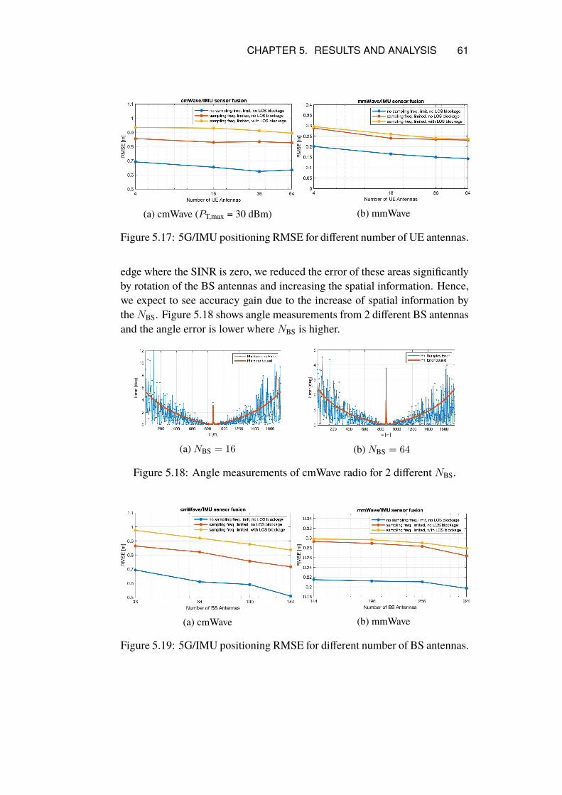
CHAPTER 5. RESULTS AND ANALYSIS 61
(a) cmWave (PT,max = 30 dBm) (b) mmWave
Figure 5.17: 5G/IMU positioning RMSE for different number of UE antennas.
edge where the SINR is zero, we reduced the error of these areas significantlyby rotation of the BS antennas and increasing the spatial information. Hence,we expect to see accuracy gain due to the increase of spatial information bytheNBS. Figure 5.18 shows angle measurements from 2 different BS antennasand the angle error is lower where NBS is higher.
(a) NBS = 16 (b) NBS = 64
Figure 5.18: Angle measurements of cmWave radio for 2 different NBS.
(a) cmWave (b) mmWave
Figure 5.19: 5G/IMU positioning RMSE for different number of BS antennas.

62 CHAPTER 5. RESULTS AND ANALYSIS
Figure 5.19 demonstrates how increasing the number of the base stationantennas NBS affects the accuracy. It can be seen that in the cmWave subsys-tem, by increasing NBS from 36 to 144, 20 cm accuracy gain is possible.

Chapter 6
Conclusions
In this project, a positioning system for vehicles based on the 5G cellular net-work and sensor fusion is developed and analyzed.
URA antennas are used in 5G network radio terminals which can providerange and angle measurements with respect to the fixed base stations. Theerror bounds of these measurements are calculated based on the CRLB the-orem. In the sensor fusion process, measurements from the cellular networkare combined with IMU acceleration measurements by an extended Kalmanfilter.
In order to study the implementation, a simple experiment is designed. Itis a straight highway where the base stations are deployed alongside of it anda car moving on a predefined trajectory is being tracked by the implementedsystem. LOS communication between the car and the cellular network can beblocked based on the static blockage models defined in the experiment. Themotion model of the car is defined with sharp turns and harsh brakes at a highvelocity to challenge the positioning system. Then, important impactive pa-rameters of the positioning system such as bandwidth, number of the antennas,number of sequential symbols, blockage specs, base stations’ distance, and etcare analyzed usingMonte Carlo experiments to show the limiting factors of thesystem.
The results show that this system can be an alternative positioning systemwhen GNSS has no coverage in the tunnels or urban canyons. Even though itis shown that rural blockage degrades the performance; however, using moreresources can compensate that.
This project is designed to study the fundamental models. Hence, real-world applicability will have to be proven in the future works. Further limita-tions and future work are presented in the subsections below.
63

64 CHAPTER 6. CONCLUSIONS
6.1 LimitationsDue to the limited time of this thesis, the work is limited in many aspects. Thelocalized objects are considered to be in xy-plane and their elevation does notchange. In the cellular network model, it is assumed that the measurementsare only available in LOS and downlink communication mode. Moreover,the CRLBs formulas used for the error bounds do not consider the estimationprocess. Hence, some negative factors such as time synchronization betweenthe transmitter and the receiver which is necessary for TOA estimation is nottaken into account. The generated measurement noise samples assumed to bei.i.d while in a real estimator this might not happen. As for the experimentalsetup, only a simple straight highway is considered, therefore, the performanceof the system in a circular highway might be different.
6.2 Future WorksSince this project was about to present a positioning system and to show itsfundamental performance, the next steps are to verify it in a more practicalway. Various future works are identified and summarized in the followingitems:
1. To make the experimental setup more accurate, the trajectory and themovement of a real car in a harsh driving scenario can be sampled bya very accurate positioning system and be used instead of the generatedtrajectory in the tests.
2. In order to get closer to the applicability, other advanced data fusionfilters instead of the Kalman filter can be used such as particle filter.
3. As mentioned in the results section, having a non-precise noise mea-surement covariance can significantly affect the system performance.To overcome this issue, an adaptive Kalman filter can be designed andimplemented or an estimation of the angle and range noise covariancebased on the SNR or even the CRLBs can be used.
4. To elaborate the work on the cellular network side, fellow researcherscan work on a cellular network model with the scheduling and powercontrol algorithms. Moreover, the angle and range estimators can beimplemented instead of using only error bounds.

Bibliography
[1] K. Ohno, T. Tsubouchi, and S. Yuta, “Outdoor map building based onodometry and rtk-gps positioning fusion”, in IEEE International Con-ference on Robotics and Automation, 2004. Proceedings. ICRA ’04.2004, vol. 1, Apr. 2004, 684–690 Vol.1. doi: 10 . 1109 / ROBOT .2004.1307228.
[2] WeiWang andDanWang, “Land vehicle navigation using odometry/ins/visionintegrated system”, in 2008 IEEE Conference on Cybernetics and In-telligent Systems, Sep. 2008, pp. 754–759. doi: 10.1109/ICCIS.2008.4670839.
[3] P. Zhang, J. Gu, E. E.Milios, and P. Huynh, “Navigationwith imu/gps/digitalcompass with unscented kalman filter”, in IEEE International Confer-ence Mechatronics and Automation, 2005, vol. 3, Jul. 2005, 1497–1502Vol. 3. doi: 10.1109/ICMA.2005.1626777.
[4] S. Kuutti, S. Fallah, K. Katsaros, M. Dianati, F. Mccullough, and A.Mouzakitis, “A Survey of the State-of-the-Art Localization Techniquesand Their Potentials for Autonomous Vehicle Applications”, IEEE In-ternet of Things Journal, vol. 5, no. 2, pp. 829–846, Apr. 2018, issn:2327-4662.doi:10.1109/JIOT.2018.2812300. [Online]. Avail-able:https://ieeexplore.ieee.org/document/8306879/(visited on 07/20/2019).
[5] X. Cui, T. A. Gulliver, J. Li, and H. Zhang, “Vehicle Positioning Us-ing 5gMillimeter-Wave Systems”, IEEE Access, vol. 4, pp. 6964–6973,2016, issn: 2169-3536. doi: 10.1109/ACCESS.2016.2615425.[Online]. Available:http://ieeexplore.ieee.org/document/7583720/ (visited on 07/20/2019).
[6] A. Kakkavas, M. H. C. Garcia, R. A. Strirling-Gallacher, and J. A.Nossek, “Performance Limits of Single-Anchormm-Wave Positioning”,arXiv:1808.08116 [cs, math], Aug. 2018, arXiv: 1808.08116. [Online].
65

66 BIBLIOGRAPHY
Available: http://arxiv.org/abs/1808.08116 (visited on03/11/2019).
[7] Z. Abu-Shaban, X. Zhou, T. Abhayapala, G. Seco-Granados, and H.Wymeersch, “Error Bounds for Uplink and Downlink 3d Localizationin 5g Millimeter Wave Systems”, IEEE Transactions on Wireless Com-munications, vol. 17, no. 8, pp. 4939–4954, Aug. 2018, issn: 1536-1276, 1558-2248. doi: 10.1109/TWC.2018.2832134. [Online].Available: https : / / ieeexplore . ieee . org / document /8356190/ (visited on 03/11/2019).
[8] A. Shahmansoori, G. E. Garcia, G. Destino, G. Seco-Granados, and H.Wymeersch, “Position and Orientation Estimation ThroughMillimeter-Wave MIMO in 5g Systems”, IEEE Transactions on Wireless Com-munications, vol. 17, no. 3, pp. 1822–1835, Mar. 2018, issn: 1536-1276, 1558-2248. doi: 10.1109/TWC.2017.2785788. [Online].Available: https : / / ieeexplore . ieee . org / document /8240645/ (visited on 07/20/2019).
[9] I. K. Jain, R. Kumar, and S. Panwar, “Driven by Capacity or Block-age? A Millimeter Wave Blockage Analysis”, in 2018 30th Interna-tional Teletraffic Congress (ITC 30), Vienna: IEEE, Sep. 2018, pp. 153–159, isbn: 978-0-9883045-5-0. doi:10.1109/ITC30.2018.00032.[Online]. Available:https://ieeexplore.ieee.org/document/8493070/ (visited on 07/21/2019).
[10] L. Jetto, S. Longhi, and G. Venturini, “Development and experimen-tal validation of an adaptive extended Kalman filter for the localiza-tion of mobile robots”, IEEE Transactions on Robotics and Automa-tion, vol. 15, no. 2, pp. 219–229, Apr. 1999, issn: 1042296X. doi: 10.1109/70.760343. [Online]. Available: http://ieeexplore.ieee.org/document/760343/ (visited on 07/21/2019).
[11] I. Siomina, A. Furuskär, and G. Fodor, “A mathematical framework forstatistical qos and capacity studies in ofdm networks”, in 2009 IEEE20th International Symposium on Personal, Indoor and Mobile RadioCommunications, Sep. 2009, pp. 2772–2776. doi: 10.1109/PIMRC.2009.5450287.
[12] P. Butovitsch and D. Astely, “White paper: Advanced antenna systemsfor 5g networks”, Ericsson AB, Tech. Rep., Nov. 2018. [Online]. Avail-able: https : / / www . ericsson . com / 4ac61a / assets /

BIBLIOGRAPHY 67
local / publications / white - papers / 10201407 _ wp _advanced_antenna_system_nov18_181115.pdf.
[13] H. Krim and M. Viberg, “Two decades of array signal processing re-search: The parametric approach”, IEEE Signal Processing Magazine,vol. 13, no. 4, pp. 67–94, Jul. 1996. doi: 10.1109/79.526899.
[14] G. R. MacCartney and T. S. Rappaport, “Study on 3gpp rural macro-cell path loss models for millimeter wave wireless communications”, in2017 IEEE International Conference on Communications (ICC), May2017, pp. 1–7. doi: 10.1109/ICC.2017.7996793.
[15] “5g; study on channel model for frequencies from 0.5 to 100 ghz (3gpptr 38.901 version 14.0.0 release 14)”, 3rdGeneration Partnership ProjectTechnical Specification Group Radio Access Network, Tech. Rep., May2017.
[16] S. M. Kay, Fundamentals of statistical signal processing, ser. Pren-tice Hall signal processing series. Upper Saddle River, NJ: PrenticeHall PTR, 1993. [Online]. Available: http://cds.cern.ch/record/2012069.
[17] R. E. Kalman, “A New Approach to Linear Filtering and PredictionProblems”, Journal of Fluids Engineering, vol. 82, no. 1, pp. 35–45,Mar. 1960, issn: 0098-2202. doi: 10.1115/1.3662552. eprint:https://asmedigitalcollection.asme.org/fluidsengineering/article- pdf/82/1/35/4756308/35\_1.pdf. [Online].Available: https://doi.org/10.1115/1.3662552.
[18] H. Bandemer, “Bibby, J., H. Toutenburg: Prediction and improved esti-mation in linearmodels. J.Wiley&Sons, Chichester-NewYork-Brisbane-Toronto 1977. 201 pp., £ 7.95: Book Review”, en, Biometrical Journal,vol. 20, no. 7-8, pp. 826–826, 1978, issn: 03233847. doi: 10.1002/bimj.197800029. [Online]. Available: http://doi.wiley.com/10.1002/bimj.197800029 (visited on 09/13/2019).
[19] Y. Bar-Shalom, X.-R. Li, and T. Kirubarajan, Estimation with applica-tions to tracking and navigation. New York: Wiley, 2001, isbn: 978-0-471-41655-5.
[20] F. Caron, E. Duflos, D. Pomorski, and P. Vanheeghe, “GPS/IMU datafusion using multisensor Kalman filtering: Introduction of contextualaspects”, en, Information Fusion, vol. 7, no. 2, pp. 221–230, Jun. 2006,issn: 15662535. doi: 10 . 1016 / j . inffus . 2004 . 07 . 002.

68 BIBLIOGRAPHY
[Online]. Available: https://linkinghub.elsevier.com/retrieve/pii/S156625350400065X (visited on 08/07/2019).
[21] V. P. J. X. Rong Li, Survey of maneuvering target tracking: Dynamicmodels, 2000. doi: 10 . 1117 / 12 . 391979. [Online]. Available:https://doi.org/10.1117/12.391979.
[22] MATLAB, version 9.6.0 (R2019a). Natick, Massachusetts: The Math-Works Inc., 2019.
[23] Automated driving toolboxTM user’s guide, English, version 2.0, TheMathworks, Inc., Natick, Massachusetts, Mar. 2019. [Online]. Avail-able: https : / / se . mathworks . com / help / releases /R2019a/pdf_doc/driving/driving_ug.pdf.
[24] X. Lin, J. Li, R. Baldemair, T. Cheng, S. Parkvall, D. Larsson, H. Koora-paty, M. Frenne, S. Falahati, A. Grövlen, and K.Werner, “5g new radio:Unveiling the essentials of the next generation wireless access technol-ogy”, Jun. 2018.
[25] E. Dahlman, S. Parkvall, and J. Skold, 5G NR - the Next GenerationWireless Access Technology: the Next GenerationWireless Access Tech-nology.English. SanDiego: Elsevier Science&Technology, 2018, OCLC:1048937251, isbn: 978-0-12-814324-7. [Online]. Available:http://public.eblib.com/choice/publicfullrecord.aspx?p=5493036 (visited on 08/02/2019).
[26] A. Devices, Accelerometer Specifications - Quick Definitions. [Online].Available: https : / / www . analog . com / en / products /landing-pages/001/accelerometer-specifications-definitions.html.
[27] Bmi055 data sheet: Small, versatile 6dof sensor module, Bosch Sen-sortecGmbH, Jul. 2014. [Online]. Available:https://www.mouser.com/ds/2/783/BST-BMI055-DS000-08-786482.pdf.
[28] A. A. Zaidi, R. Baldemair, H. Tullberg, H. Bjorkegren, L. Sundstrom,J. Medbo, C. Kilinc, and I. Da Silva, “Waveform and Numerology toSupport 5g Services and Requirements”, IEEE Communications Mag-azine, vol. 54, no. 11, pp. 90–98, Nov. 2016, issn: 0163-6804. doi:10.1109/MCOM.2016.1600336CM. [Online]. Available: http://ieeexplore.ieee.org/document/7744816/ (visited on08/02/2019).

BIBLIOGRAPHY 69
[29] “5g;study on scenarios and requirements for next generation access tech-nologies (3gpp tr 38.913 version 14.3.0 release 14)”, 3rd GenerationPartnership Project Technical Specification Group Radio Access Net-work, Tech. Rep., 2017.
[30] S. Ahmadi, Ed., 5G NR: architecture, technology, implementation, andoperation of 3gpp new radio standards. Cambridge: Elsevier, 2019,isbn: 978-0-08-102267-2.


www.kth.seTRITA-EECS-EX-2019:672