vehicle routing for emergency evacuations · vehicle routing problem motivated both by its...
TRANSCRIPT

Vehicle Routing for Emergency Evacuations
Victor Caon Pereira
Dissertation submitted to the faculty of the
Virginia Polytechnic Institute and State University
in partial fulfillment of the requirements for the degree of
Doctor of Philosophy
in
Industrial and Systems Engineering
Douglas R. Bish, Chair
Kimberly P. Ellis
Barbara M. Fraticelli
Subhash C. Sarin
Gaylon D. Taylor Jr.
October 29, 2013
Blacksburg, Virginia
Keywords: Emergency Evacuations, Vehicle Routing Problem, Mixed-Integer Quadratic
Programming, Ritter Relaxation, Dynamic Vehicle Routing Problem
Vehicle Routing for Emergency Evacuations
Victor Caon Pereira
(ABSTRACT)
This dissertation introduces and analyzes the Bus Evacuation Problem (BEP), a unique
Vehicle Routing Problem motivated both by its humanitarian significance and by the routing
and scheduling challenges of planning transit-based, regional evacuations. First, a variant
where evacuees arrive at constant, location-specific rates is introduced. In this problem, a
fleet of capacitated buses must transport all evacuees to a depot/shelter such that the last
scheduled pick-up and the end of the evacuee arrival process occurs at a location-specific
time. The problem seeks to minimize their accumulated waiting time, restricts the number
of pick-ups on each location, and exploits efficiencies from service choice and from allowing
buses to unload evacuees at the depot multiple times. It is shown that, depending on the
problem instance, increasing the maximum number of pick-ups allowed may reduce both
the fleet size requirement and the evacuee waiting time, and that, past a certain threshold,
there exist a range of values that guarantees an efficient usage of the available fleet and
equitable reductions in waiting time across pick-up locations. Second, an extension of the
Ritter (1967) Relaxation Algorithm, which explores the inherent structure of problems with
complicating variables and constraints, such as the aforementioned BEP variant, is presented.
The modified algorithm allows problems with linear, integer, or mixed-integer subproblems
and with linear or quadratic objective functions to be solved to optimality. Empirical studies

demonstrate the algorithm viability to solve large optimization problems. Finally, a two-stage
stochastic formulation for the BEP is presented. Such variant assumes that all evacuees are
at the pick-up locations at the onset of the evacuation, that the set of possible demands
is provided, and, more importantly, that the actual demands become known once buses
visit the pick-up locations for the first time. The effect of exploratory visits (sampling) and
symmetry is explored, and the resulting insights used to develop an improved formulation
for the problem. An iterative (dynamic) solution algorithm is proposed.
This work has been supported by the National Science Foundation under Award Numbers
0825611 and 1055360.
iii

Dedication
This work is dedicated to my loving wife, Carolina, to my daughter, Vivian, and to my
parents, Rodinei and Telma. Without their love and unwavering support, I would not have
been able to finish this monumental task.
iv

Acknowledgments
I would like to thank my advisor and mentor, Dr. Douglas Bish, for inspiring me to reach
for excellence in my work, for allowing me to pursue this challenging research topic, and
for the countless hours spent reading, reflecting, and guiding me throughout this process. I
would like to thank my committee members, Dr. Kimberly Ellis, Dr. Barbara Fraticelli, Dr.
Subhash Sarin, and Dr. Don Taylor, for their enlightening insights and encouraging words.
Not only were their comments instrumental in shaping this research, but they also kept me
focused, motivated, and enthusiastic about my research. I would like to thank the Industrial
and Systems Engineering Graduate Program Coordinator, Mrs. Hanna Parks, for helping
me navigate through every Department and Graduate School procedure, and for ensuring
that I would meet all the enrollment, academic progress, and graduation requirements and
deadlines. I would like to thank my fellow graduate students for fostering an atmosphere
of respect, friendship, and mutual support. Their valuable, and often impromptu advice,
significantly eased these strenuous years of graduate education. I would like to thank the
dedicated and caring faculty and staff of Virginia Tech for generously sharing their time and
expertise. Finally, I would like to thank Virginia Tech, the Graduate School, the College of
v

Engineering, and, in particular, the Grado Department of Industrial and Systems Engineer-
ing, for providing me the resources needed to complete this work, ample opportunities to
learn, and a supportive and collaborative environment.
This has been a challenging and rewarding experience. Thank you all for this once in a
lifetime opportunity!
vi
Contents
1 Introduction 1
1.1 Motivation . . . . . . . . . . . . . . . . . . . . . . . . . . . . . . . . . . . . . 2
1.2 Problem Description . . . . . . . . . . . . . . . . . . . . . . . . . . . . . . . 4
1.3 Literature Review . . . . . . . . . . . . . . . . . . . . . . . . . . . . . . . . . 7
1.3.1 The Vehicle Routing Problem . . . . . . . . . . . . . . . . . . . . . . 7
1.3.2 The Bus Evacuation Problem . . . . . . . . . . . . . . . . . . . . . . 12
1.3.3 Conclusions from the Literature Review . . . . . . . . . . . . . . . . 25
1.4 Solution Methodologies . . . . . . . . . . . . . . . . . . . . . . . . . . . . . . 33
1.4.1 Exact Algorithms . . . . . . . . . . . . . . . . . . . . . . . . . . . . . 33
1.4.1.1 The k-Degree Center Tree Algorithm . . . . . . . . . . . . . 33
1.4.1.2 Set Partitioning and Column Generation . . . . . . . . . . . 37
1.4.2 Heuristics . . . . . . . . . . . . . . . . . . . . . . . . . . . . . . . . . 40
1.4.2.1 The Savings Algorithm . . . . . . . . . . . . . . . . . . . . . 40
1.4.2.2 The Sweep Algorithm . . . . . . . . . . . . . . . . . . . . . 42
1.4.3 Metaheuristics . . . . . . . . . . . . . . . . . . . . . . . . . . . . . . . 44
1.4.3.1 Simulated Annealing . . . . . . . . . . . . . . . . . . . . . . 44
1.4.3.2 Genetic Approaches . . . . . . . . . . . . . . . . . . . . . . 46
1.4.3.3 Tabu Search . . . . . . . . . . . . . . . . . . . . . . . . . . . 49
1.4.3.4 Ant Colony Optimization . . . . . . . . . . . . . . . . . . . 51
1.4.4 Summary of Solution Algorithms . . . . . . . . . . . . . . . . . . . . 53
vii
2 Scheduling and Routing for a Bus-based Evacuation with Constant Evac-uee Arrival Rate 56
2.1 Introduction . . . . . . . . . . . . . . . . . . . . . . . . . . . . . . . . . . . . 58
2.2 Modeling Framework . . . . . . . . . . . . . . . . . . . . . . . . . . . . . . . 64
2.3 Model Analysis . . . . . . . . . . . . . . . . . . . . . . . . . . . . . . . . . . 69
2.3.1 The Maximum Service Level . . . . . . . . . . . . . . . . . . . . . . . 70
2.3.1.1 Service Choice. . . . . . . . . . . . . . . . . . . . . . . . . . 71
2.3.1.2 The Minimum Exposure Schedule. . . . . . . . . . . . . . . 76
2.3.2 Fleet Size . . . . . . . . . . . . . . . . . . . . . . . . . . . . . . . . . 82
2.3.2.1 Minimum Fleet Size. . . . . . . . . . . . . . . . . . . . . . . 83
2.3.2.2 Upper Bound on the MES(F ) Fleet Size. . . . . . . . . . . 84
2.3.2.3 Lower Bound on the MES(F ) Fleet Size. . . . . . . . . . . 85
2.3.2.4 The MES(F ) Fleet Size. . . . . . . . . . . . . . . . . . . . 87
2.3.2.5 Upper Bound on the BEP-CA Fleet Size. . . . . . . . . . . 94
2.3.2.6 Lower Bound on the BEP-CA Fleet Size. . . . . . . . . . . . 96
2.3.3 Upper Bound on the Maximum Number of Arc Traversals per Vehicle 100
2.4 Conclusions and Further Research . . . . . . . . . . . . . . . . . . . . . . . . 104
2.5 Appendix . . . . . . . . . . . . . . . . . . . . . . . . . . . . . . . . . . . . . 106
3 A Variant of the Ritter Relaxation Algorithm Applied to Problems withMixed-Integer Subproblems and Linear or Quadratic Objective Functions115
3.1 Introduction . . . . . . . . . . . . . . . . . . . . . . . . . . . . . . . . . . . . 116
3.2 The Ritter (1967) Relaxation Algorithm . . . . . . . . . . . . . . . . . . . . 118
3.2.1 Original Algorithm . . . . . . . . . . . . . . . . . . . . . . . . . . . . 119
3.2.2 Modified Algorithm . . . . . . . . . . . . . . . . . . . . . . . . . . . . 130
3.3 Empirical Studies . . . . . . . . . . . . . . . . . . . . . . . . . . . . . . . . . 147
3.4 Conclusions and Future Research . . . . . . . . . . . . . . . . . . . . . . . . 150
3.5 Appendix . . . . . . . . . . . . . . . . . . . . . . . . . . . . . . . . . . . . . 152
4 The Dynamic Bus Evacuation Problem with Stochastic Customers and
viii
Demand 158
4.1 Introduction . . . . . . . . . . . . . . . . . . . . . . . . . . . . . . . . . . . . 160
4.2 Modeling Framework . . . . . . . . . . . . . . . . . . . . . . . . . . . . . . . 167
4.2.1 Two-Stage Stochastic Formulation . . . . . . . . . . . . . . . . . . . . 168
4.2.2 Iterative Algorithm for the Stochastic Formulation . . . . . . . . . . 171
4.3 Problem Analysis . . . . . . . . . . . . . . . . . . . . . . . . . . . . . . . . . 178
4.3.1 The Effect of Sampling . . . . . . . . . . . . . . . . . . . . . . . . . . 179
4.3.2 The Effect of Symmetry . . . . . . . . . . . . . . . . . . . . . . . . . 182
4.3.3 Deterministic Formulation . . . . . . . . . . . . . . . . . . . . . . . . 184
4.3.4 Iterative Algorithm for the Deterministic Formulation . . . . . . . . . 190
4.3.5 Algorithm Comparison . . . . . . . . . . . . . . . . . . . . . . . . . . 195
4.4 Conclusion and Future Research . . . . . . . . . . . . . . . . . . . . . . . . . 199
5 Conclusions 202
References 210
Appendix A Summary of the Bus Evacuation Problem Literature Review 224
Appendix B Alternative Formulations for the Bus Evacuation Problem withConstant Evacuee Arrival Rate 231
B.1 Original Formulation in Standard Form . . . . . . . . . . . . . . . . . . . . . 232
B.2 Alternate Formulation I . . . . . . . . . . . . . . . . . . . . . . . . . . . . . 238
B.3 Alternate Formulation II . . . . . . . . . . . . . . . . . . . . . . . . . . . . . 242
B.4 Alternate Formulation III . . . . . . . . . . . . . . . . . . . . . . . . . . . . 244
Appendix C Numerical Examples of the Original and Modified Ritter (1967)Relaxation Algorithms 248
C.1 Example Problem . . . . . . . . . . . . . . . . . . . . . . . . . . . . . . . . . 249
C.2 A Numerical Example of the Ritter (1967) Relaxation Algorithm . . . . . . . 250
C.3 A Numerical Example of the Ritter (1967) Relaxation Algorithm Without theSwapping Operation . . . . . . . . . . . . . . . . . . . . . . . . . . . . . . . 263
ix

C.4 A Numerical, Integer Example of the Ritter (1967) Relaxation AlgorithmWithout the Swapping Operation . . . . . . . . . . . . . . . . . . . . . . . . 272
C.5 A Numerical, Mixed-Integer Example of the Ritter (1967) Relaxation Algo-rithm Without the Swapping Operation . . . . . . . . . . . . . . . . . . . . . 282
C.6 A Numerical, Mixed-Integer, Quadratic Example of the Ritter (1967) Relax-ation Algorithm Without the Swapping Operation . . . . . . . . . . . . . . . 295
Appendix D The Ritter (1967) Relaxation Algorithm - Source Code: Math-Works Matlab version R2012a (7.14.0.739) 309
D.1 Original Algorithm . . . . . . . . . . . . . . . . . . . . . . . . . . . . . . . . 310
D.2 Modified Algorithm . . . . . . . . . . . . . . . . . . . . . . . . . . . . . . . . 335
Appendix E Iterative Algorithm for the D-VRP Variation of the BEP -Source Code: IBM ILOG CPLEX Optimization Studio version 12.5 366
E.1 Two-Stage Stochastic Formulation . . . . . . . . . . . . . . . . . . . . . . . . 367
E.1.1 Model File (BaseModel.mod) . . . . . . . . . . . . . . . . . . . . . . 367
E.1.2 Data File (BaseModel.dat) . . . . . . . . . . . . . . . . . . . . . . . . 369
E.1.3 Iterative Algorithm (BaseModelLoop.mod) . . . . . . . . . . . . . . . 370
E.2 Deterministic Formulation . . . . . . . . . . . . . . . . . . . . . . . . . . . . 377
E.2.1 Model File (EnhancedModel.mod) . . . . . . . . . . . . . . . . . . . . 377
E.2.2 Data File (EnhancedModel.dat) . . . . . . . . . . . . . . . . . . . . . 379
E.2.3 Iterative Algorithm (EnhancedModelLoop.mod) . . . . . . . . . . . . 380
x
List of Figures
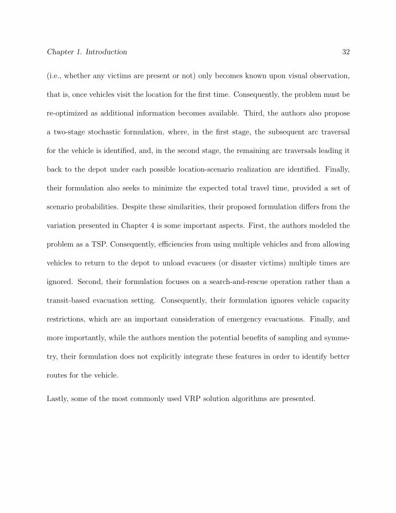
1.1 An example optimum solution for a m-TSP with 2 routes. . . . . . . . . . . 34
1.2 An example optimum partition for the k-degree center tree algorithm. . . . . 35
1.3 Conceptualization of the savings algorithm, before (a) and after (b) individualcircuits are merged. . . . . . . . . . . . . . . . . . . . . . . . . . . . . . . . . 41
1.4 An example optimum solution for the Sweep Algorithm . . . . . . . . . . . . 43
1.5 An example of crossover under the Genetic Algorithm. . . . . . . . . . . . . 47
1.6 An example of mutation under the Genetic Algorithm. . . . . . . . . . . . . 48
2.1 The networks for Scenarios 1 (a) and 2 (b). . . . . . . . . . . . . . . . . . . . 68
2.2 An example network (a) and representations of the corresponding optimalpick-up schedules without service choice (b), and with service choice (c). . . 72
2.3 An example network (a) and representations of the corresponding optimalpick-up schedules for F = 2 (b) and F = 3 (c) pick-ups. . . . . . . . . . . . . 74
2.4 Evacuees waiting at pick-up node 1, Scenario 1 (a) and corresponding exposure(b) for the MES(F ) for F = 2, F = 5, and F = 15. . . . . . . . . . . . . . . 78
2.5 MES(F ) total exposure as a function of F and limiting exposure for Scenarios1 and 2. . . . . . . . . . . . . . . . . . . . . . . . . . . . . . . . . . . . . . . 79
2.6 An example network (a) and representations of the corresponding optimalpick-up schedules for F = 1 (b) and F = 2 (c) pick-ups. . . . . . . . . . . . . 81
2.7 An example network (a) and representations of the corresponding MES(F )for F = 2 (b) and F = 5 (c). . . . . . . . . . . . . . . . . . . . . . . . . . . . 86
2.8 Representations of the MES(F ) for F = 1 (a) and F = 3 (b) correspondingto the network presented in Example 2.4, Figure 2.7(a). . . . . . . . . . . . . 88
xi
2.9 Upper bound, lower bound, and the exact fleet size needed for a feasibleimplementation of the MES(F ) by the maximum service level for Scenarios1 (a) and 2 (b). . . . . . . . . . . . . . . . . . . . . . . . . . . . . . . . . . . 89
2.10 Conceptualization of the upper and lower bounds on the fleet size needed fora feasible implementation of the MES(F ) and its corresponding total exposure. 92
2.11 Representations of the optimal pick-up schedule for F = 3, V = 1, corre-sponding to the network presented in Example 2.4, Figure 2.7(a). . . . . . . 95
2.12 Upper bound, lower bound, and the exact fleet size needed for a feasiblesolution to the problem by the maximum service level for Scenarios 1 (a) and2 (b). . . . . . . . . . . . . . . . . . . . . . . . . . . . . . . . . . . . . . . . . 97
2.13 The minimum exposure by fleet size and by maximum service level for Sce-narios 1 (a) and 2 (b) for F = 1, · · · , 4. All remaining data is extrapolated. . 98
2.14 T (F ), as obtained from the MIP formulation, from the upper bound proce-dure, and the minimum value needed for a feasible implementation of theMES(F ) by maximum service level for Scenarios 1 (a) and 2 (b). . . . . . . 104
3.1 A representation of the scheme used to partition the original Hessian matrix. 137
4.1 Flowchart of the iterative algorithm for the stochastic formulation. . . . . . . 172
4.2 An example network for the algorithm implementation. . . . . . . . . . . . . 174
4.3 A conceptual network for the exemplification of sampling and symmetry. . . 179
4.4 Flowchart of the iterative algorithm for the deterministic formulation. . . . . 192
4.5 An example network for the algorithm comparison. . . . . . . . . . . . . . . 196
B.1 An example network (a), a representation of the corresponding optimal pick-up schedule for F = 2 pick-ups assuming the possibility of transit corridors(b) and assuming that these are disallowed (c). . . . . . . . . . . . . . . . . . 241
C.1 First iteration of the branch and bound algorithm. . . . . . . . . . . . . . . . 287
C.2 Second iteration of the branch and bound algorithm. . . . . . . . . . . . . . 288
C.3 Third iteration of the branch and bound algorithm. . . . . . . . . . . . . . . 289
C.4 Fourth iteration of the branch and bound algorithm. . . . . . . . . . . . . . 291
C.5 Fourth iteration of the branch and bound algorithm, after a new non-negativity restriction is enforced. . . . . . . . . . . . . . . . . . . . . . . . . 292
xii
C.6 Fifth iteration of the branch and bound algorithm. . . . . . . . . . . . . . . 294
C.7 First iteration of the branch and bound algorithm. . . . . . . . . . . . . . . . 306
C.8 First iteration of the branch and bound algorithm, after the non-negativityrestriction on x1 is enforced. . . . . . . . . . . . . . . . . . . . . . . . . . . . 308
xiii
List of Tables
1.1 Contributions of the BEP variant presented in Chapter 2 . . . . . . . . . . . 28
2.1 Decision variables for the BEP-CA. . . . . . . . . . . . . . . . . . . . . . . . 65
2.2 Decision variables for the T (F ) MIP. . . . . . . . . . . . . . . . . . . . . . . 100
3.2 Wall-clock time (seconds) comparison of the Modified Ritter (1967) RelaxationAlgorithm and IBM ILOG CPLEX for various bordered-structure, MIQPproblems. . . . . . . . . . . . . . . . . . . . . . . . . . . . . . . . . . . . . . 148
4.1 Decision variables for the two-stage stochastic formulation. . . . . . . . . . . 168
4.2 Solution for each scenario of Example 4.1 on the first iteration of the algorithm.175
4.3 Solution for each scenario of Example 4.1 on the second iteration of the algo-rithm. . . . . . . . . . . . . . . . . . . . . . . . . . . . . . . . . . . . . . . . 176
4.4 Solution for each scenario of Example 4.1 on the third iteration of the algorithm.177
4.5 Symmetrical solutions for the network presented in Figure 4.3. . . . . . . . . 183
4.6 Decision variables for the deterministic formulation. . . . . . . . . . . . . . . 187
4.7 Example scenarios for the network depicted in Figure 4.5. . . . . . . . . . . . 197
A.1 Summary of the Bus Evacuation Problem literature review . . . . . . . . . . 225
A.2 Summary of the Bus Evacuation Problem literature review (continued) . . . 228
B.1 Decision variables for the BEP variant introduced in Chapter 2. . . . . . . . 233
B.2 Slack variables for the formulation introduced in Chapter 2. . . . . . . . . . 234
B.3 Comparison of the alternate formulations for the BEP by problem size. . . . 247
xiv
List of Abbreviations
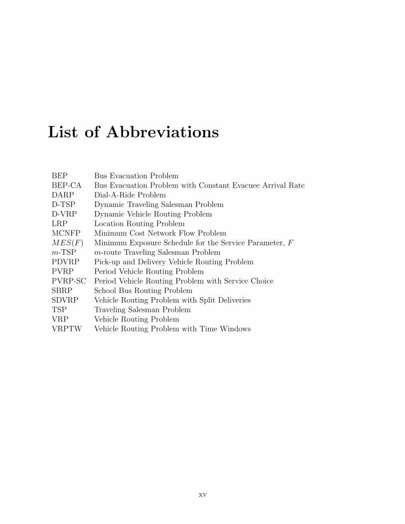
BEP Bus Evacuation ProblemBEP-CA Bus Evacuation Problem with Constant Evacuee Arrival RateDARP Dial-A-Ride ProblemD-TSP Dynamic Traveling Salesman ProblemD-VRP Dynamic Vehicle Routing ProblemLRP Location Routing ProblemMCNFP Minimum Cost Network Flow ProblemMES(F ) Minimum Exposure Schedule for the Service Parameter, Fm-TSP m-route Traveling Salesman ProblemPDVRP Pick-up and Delivery Vehicle Routing ProblemPVRP Period Vehicle Routing ProblemPVRP-SC Period Vehicle Routing Problem with Service ChoiceSBRP School Bus Routing ProblemSDVRP Vehicle Routing Problem with Split DeliveriesTSP Traveling Salesman ProblemVRP Vehicle Routing ProblemVRPTW Vehicle Routing Problem with Time Windows
xv
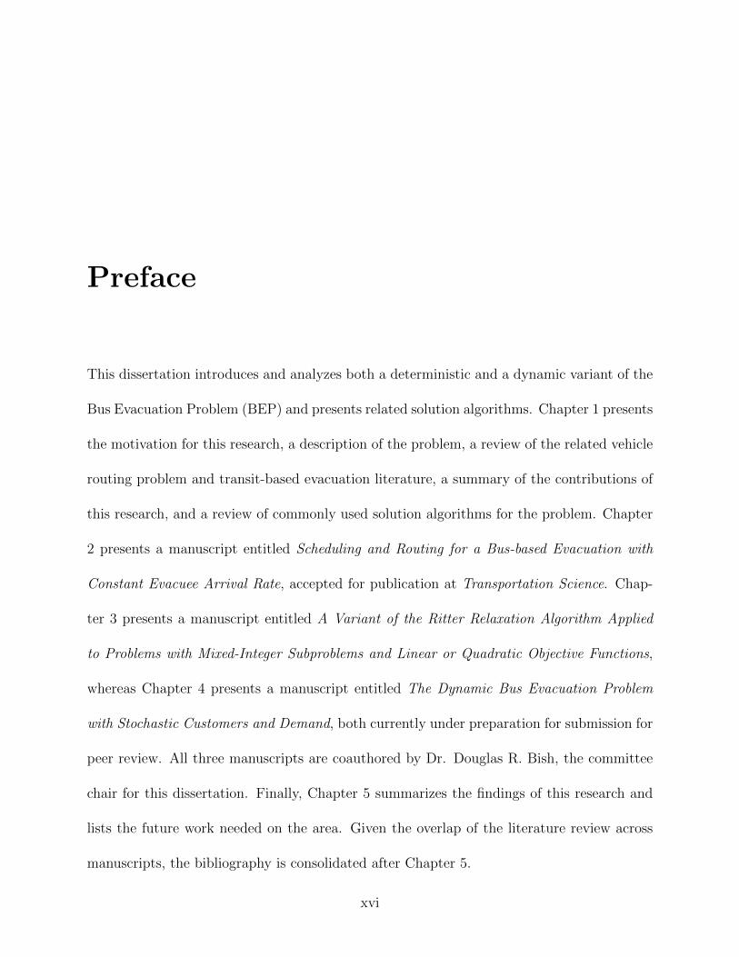
Preface
This dissertation introduces and analyzes both a deterministic and a dynamic variant of the
Bus Evacuation Problem (BEP) and presents related solution algorithms. Chapter 1 presents
the motivation for this research, a description of the problem, a review of the related vehicle
routing problem and transit-based evacuation literature, a summary of the contributions of
this research, and a review of commonly used solution algorithms for the problem. Chapter
2 presents a manuscript entitled Scheduling and Routing for a Bus-based Evacuation with
Constant Evacuee Arrival Rate, accepted for publication at Transportation Science. Chap-
ter 3 presents a manuscript entitled A Variant of the Ritter Relaxation Algorithm Applied
to Problems with Mixed-Integer Subproblems and Linear or Quadratic Objective Functions,
whereas Chapter 4 presents a manuscript entitled The Dynamic Bus Evacuation Problem
with Stochastic Customers and Demand, both currently under preparation for submission for
peer review. All three manuscripts are coauthored by Dr. Douglas R. Bish, the committee
chair for this dissertation. Finally, Chapter 5 summarizes the findings of this research and
lists the future work needed on the area. Given the overlap of the literature review across
manuscripts, the bibliography is consolidated after Chapter 5.
xvi
Chapter 1
Introduction
1

Chapter 1. Introduction 2
This Chapter discusses the humanitarian significance of transit-based regional evacuation
planning and implementation, provides a description of the Bus Evacuation Problem (BEP),
reviews the related Vehicle Routing Problem (VRP) and the modeling and optimization
literature, and summarizes the contributions of this research as it relates to advances in
problem formulation and solution methodology. Lastly, a review of commonly used solution
algorithms for the problem is presented.
1.1 Motivation
Most of the planning emphasis for large-scale, regional evacuations is automobile-centric
(U.S. Department of Homeland Security, 2006). While such is an extremely important aspect
of disaster preparedness, there can be a large segment of the population without access to
automobiles, and, consequently, without the means to leave the disaster area. For example,
it is estimated that between 200,000 and 300,000 people in New Orleans (approximately 27%
of its households) did not have access to any reliable means of personal transportation prior
to Hurricane Katrina’s landfall in 2005 (Wolshon, 2002; Hess and Gotham, 2007). On its
aftermath, between 100,000 and 120,000 residents, most of which were poor and belonging to
minorities, remained in the city, risk exposed, and later became the second wave of evacuees
(Nigg et al., 2006). Similarly, Hess and Gotham (2007), while reviewing the evacuation
plans from cities in the State of New York (excluding Long Island and the five counties
comprising New York City), concluded that many of those cities either meet or exceed New
Chapter 1. Introduction 3
Orleans percentage of households without access to automobiles. In fact, 9.1% of all occupied
housing units in the United States (approximately 10.5 million homes) currently lack any
form of personal transportation (U.S. Census Bureau, 2011).
Unfortunately, not only is the size of the population lacking automobiles significant, but
few regions are prepared for their mass evacuation. According to a survey conducted by
the U.S. Department of Homeland Security (2006), only 9 States and 5 of the 75 largest
urban centers of the United States sufficiently consider all modes of transportation in their
evacuation plans. Similarly, Hess and Gotham (2007) determined that upstate New York, a
rural area and site of many nuclear reactors, has a considerably large carless population, but
is insufficiently prepared for their mass evacuation in case of natural or man-made disasters.
Finally, while buses are often the most readily available and the most flexible mode of public
transport, their number is limited, and often insufficient to transport all evacuees to a safe
destination in a single trip. In fact, the 500 buses available for the evacuation of New Orleans
would only have sufficed provided their adequate routing during the 48 hours of advanced
notice (Litman, 2006). Clearly, transit-based, regional evacuation plans capable of meeting
the usually tight deadlines and of using the available resources efficiently are an essential
component of disaster preparedness.

Chapter 1. Introduction 4
1.2 Problem Description
The BEP is a variant of the VRP motivated both by its humanitarian significance and by the
routing and scheduling challenges involved in planning transit-based, regional evacuations.
In summary, the BEP aims to identify a timetable of pick-ups and the routes for a fleet of
buses to transport all carless evacuees of a region from a set of neighborhood pick-up locations
(or bus stops) to one or more shelters, while optimizing some evacuation-specific objective
function (often minimization of the evacuation completion time). Although this research
focuses on bus-based evacuations, the concepts herein developed are readily applicable to
any other mass transit vehicle, and, possibly, to alternative VRP settings.
Chapter 2 and Appendix B present multiple formulations for a BEP variant which seeks to
minimize the amount time that evacuees must wait at the pick-up locations before boarding
a transit vehicle. These formulations assume that evacuees arrive at constant, location-
specific rates, from the start of the evacuation to a location-specific end-time (aiming to
mitigate evacuation risks). Moreover, they allow vehicles to visit the depot multiple times to
unload evacuees and include spatial-temporal vehicle synchronization of pick-up times. Such
constraints coordinate the number of vehicles and the time when these depart the pick-up
locations, ensure that these have enough free capacity to accommodate all evacuees gathered
since the last scheduled pick-up time, and force at least one pick-up to take place on each
location, scheduled for the end of the evacuee arrival process. Efficiencies from allowing
fewer than a limiting number of pick-ups (service choice) are exploited. Consequently, the
Chapter 1. Introduction 5
problem ensures that every evacuee boards a transit vehicle on or before the evacuation
end-time. It is shown that, depending on the problem instance, restricting the maximum
number of pick-ups on each location may lead to an efficient usage of the available fleet, to
more equitable pick-up schedules across locations, and to an improved problem tractability.
While the BEP is often solved during the planning phase of the evacuation, reducing its
computation time is still desirable, as it allows larger problem instances to be assessed or
the model sensitivity to the input parameters to be analyzed. Unfortunately, given its com-
plexity, currently, only small instances of the aforementioned BEP variant can be solved
to optimality under reasonable time. Motivated by the need to improve its solving time,
Chapter 3 introduces an exact optimization algorithm based on a less known relaxation
methodology originally developed by Ritter (1967). The algorithm was selected due to its
ability to explore the inherent structure of problems with both complicating variables and
constraints, such as the aforementioned BEP variant, without the need to compound multiple
decomposition/relaxation strategies. The modifications proposed require fewer matrix ma-
nipulations and fewer numerical comparisons, thus leading to improved numerical stability.
In addition, the modified algorithm is combined with the branch and bound algorithm, thus
allowing bordered (or arrowhead) structure problems with linear, integer, or mixed-integer
subproblems and with linear or quadratic objective functions to be solved to optimality.
While the algorithm is not employed to solve actual instances of the aforementioned BEP
variant, empirical studies demonstrate its viability to solve large optimization problems.
Finally, Chapter 4 presents a two-stage stochastic formulation for the BEP with uncertain

Chapter 1. Introduction 6
demand. The problem assumes that all evacuees are at the pick-up locations at the onset of
the evacuation, that the fleet has homogeneous capacity, that the set of possible demands
(scenarios) on each pick-up location are provided, and that these location-scenario demands
are functions (potentially multiples) of the vehicle capacities. The first stage of the proposed
two-stage stochastic formulation seeks the subsequent arc traversal for each vehicle, common
across scenarios, whereas the second stage identifies the remaining optimal tours under each
location-scenario demand realization, starting from the respective destination nodes identi-
fied by the first stage. The problem seeks the first stage decision (i.e., the subsequent arc
traversal for each vehicle) that minimizes the expected total travel cost of the fleet, while
ensuring that every evacuee is rescued under each location-scenario demand realization.
In addition, the problem assumes that any demand uncertainty is resolved upon visual
observation, that is, once a bus visits the respective pick-up location for the first time.
A solution algorithm that iteratively re-optimizes the problem as additional information
becomes available is proposed. The algorithm terminates once every pick-up location has
been visited, and, thus, once all uncertainty has been cleared. The effect of exploratory visits
or sampling (i.e., visits to pick-up locations with the sole purpose of ascertain the realized
demand) and of symmetrical tours is explored, and the resulting insights used to develop a
more efficient problem formulation.
The next section presents a review of the related VRP and BEP literature.

Chapter 1. Introduction 7
1.3 Literature Review
1.3.1 The Vehicle Routing Problem
As aforementioned, the BEP is a variant of the VRP. In summary, the VRP aims to identify
the routes for a fleet of vehicles that minimize the accumulated cost of each vehicle’s arc
traversals, while ensuring that every customer is visited exactly once and that every vehicle
starts and ends its route at a depot (Toth and Vigo, 1998). Since the first related paper
from Dantzig et al. (1954), the VRP literature has grown exponentially, evolving into spe-
cific instances that include multiple depots, capacitated vehicles, multiple trips per vehicle,
split deliveries, time windows per customer, service choice, and backhauls. Eksioglu et al.
(2009) present an overview of the VRP literature and propose a methodology for its classifi-
cation, while Laporte (1992) presents three exact algorithms (direct enumeration, dynamic
programming, and branch and bound) and four heuristics (the savings algorithm, the sweep
algorithm, the k-degree center tree algorithm, and the tabu search algorithm) for solving the
problem.
All BEP variants presented and analyzed in this research share characteristics with specific
variations of the VRP such as the School Bus Routing Problem (SBRP) and the Dial-A-
Ride Problem (DARP). However, the variation presented in Chapter 2 is, perhaps, more
closely related to the Period Vehicle Routing Problem (PVRP), and, in particular, to the
Period Vehicle Routing Problem with Service Choice (PVRP-SC), whereas the one presented
in Chapter 4 is more closely related to the Stochastic Dynamic Vehicle Routing Problem
Chapter 1. Introduction 8
(stochastic D-VRP).
The SBRP, introduced by Newton and Thomas (1969), aims to find a school bus loading
pattern and a timetable of pick-ups that minimize total operating costs and passenger travel
times, while enforcing fleet size and bus capacity restrictions (Angel et al., 1972). Park
and Kim (2010) present a comprehensive review of the SBRP and propose a classification
methodology for the problem. Similar to the SBRP, the proposed BEP variants are con-
strained by bus loading capacities, the fact that all pick-up locations must be visited, that all
passengers must be accommodated, and that vehicles must start and end their route at the
depot (school). However, while the SBRP enforces a single pick-up by a single bus on each
location, the proposed BEP variants allow split deliveries and multiple pick-ups at the same
location. Moreover, while the SBRP restricts the overall drop-off time of students (based on
the start time of classes), the BEP variant presented in Chapter 2 restricts the last pick-up
time on each location (aiming to mitigate evacuation risks), whereas the one presented in
Chapter 4 restricts neither the last pick-up or drop-off time.
The DARP, introduced by Wilson et al. (1971), generalizes other variations of the VRP such
as the Pick-up and Delivery Vehicle Routing Problem (PDVRP) and the Vehicle Routing
Problem with Time Windows (VRPTW). The problem seeks the routes and schedules for
a fleet of homogeneous vehicles operating from a central depot to transport customers from
a set of pick-up to a set of drop-off locations, while minimizing either service cost or cus-
tomer waiting and riding time. Cordeau and Laporte (2003) describe the DARP, review
the related literature, and provide a discussion on the modeling issues and future research
Chapter 1. Introduction 9
needs. Although the proposed BEP variants do not specifically incorporate service time, a
customer-focused objective function, namely the minimization of evacuee waiting time at
the various pick-up locations, is presented in Chapter 2.
The PVRP was first mathematically formulated by Christofides and Beasley (1984). In this
problem, routes are constructed over multiple-days as opposed to the single-day case of the
ordinary VRP. Each customer requires a fixed number of visits during the period, and, on
each day, a set of capacitated buses becomes available to meet their demand. Francis et al.
(2006) offer a variation of the PVRP by introducing service choice as a decision variable,
namely the PVRP-SC. The problem seeks the routes for a fleet of vehicles operating from
a central depot such that each customer is visited, at least, a minimum number of times
in order to meet their demand. Although the problem also enforces a maximum number of
visits before a predetermined end-time, operational efficiencies and increased service benefits
may be gained by allowing customers to be visited more often than their minimum required
frequencies. For instance, suppose that two customers must be served at least twice and no
more than four times during a period of one workweek, and that a single vehicle is available
and is limited to three visits per customer over the same period. Then, one solution would be
to visit one customer on Monday and Tuesday and the other on Wednesday, Thursday and
Friday. Despite its similarities with the spatial-temporal vehicle synchronization constraints
of the BEP variant presented in Chapter 2, the PVRP-SC assumes that the set of potential
arrival times is both discrete and finite. Conversely, the BEP variant of Chapter 2 allows
visits to occur anytime before the evacuation end-time, thus extending the PVRP-SC to
Chapter 1. Introduction 10
continuous arrival times.
Finally, Chapter 4 presents a variation of the D-VRP applied to the BEP. The origins of
the D-VRP can be traced to Wilson and Colvin (1977), who proposed a DARP variation in
which customer requests for trips arrive dynamically (i.e., after vehicles begin their tour).
According to Pillac et al. (2013), unlike traditional VRPs, the D-VRP is based on the
premise that either the problem parameters change or their uncertainty is resolved after the
originally planned tours begin to be implemented. Consequently, the problem allows factors
initially unknown to the planner to be incorporated into the final solution, thus potentially
reducing operational costs, improving customer service, and even reducing environmental
impact (Pillac et al., 2013). Since the originally planned routes must be re-optimized to
account for the new information, the D-VRP often consists of a sequence of static VRPs.
The D-VRP literature is extensive, and the original problem has grown to include not only
dynamic demand, but also dynamic travel time and fleet availability (See Larsen et al., 2007;
Pillac et al., 2013, for a comprehensive review of the D-VRP literature).
Among the many variations of the D-VRP, the formulation presented in Chapter 4 more
closely resembles the stochastic D-VRP. The stochastic D-VRP is similar to its deterministic
counterpart in the sense that some of the parameters (in this case, the number of full bus
loads needed to accommodate every evacuee present at a pick-up location) are unknown a
priori and reveled dynamically during the route execution (in this case, as vehicles visit the
pick-up locations for the first time). However, contrary to its deterministic counterpart, the
problem exploits the known stochastic nature of demands to determine the arc traversals
Chapter 1. Introduction 11
more likely to result in better objective function values.
As aforementioned, the formulation presented in Chapter 4 accounts for the stochastic na-
ture of the demand on each pick-up location by formulating the problem as a two-stage
stochastic VRP. The origins of stochastic VRP with uncertain demand can be traced to
Tillman (1969), who introduce the problem and propose a solution methodology based on a
variation of the savings algorithm. Gendreau et al. (1996) present an overview of Stochastic
VRPs and a review of the related literature, whereas Louveaux and Schultz (2003) identify
several structural properties of stochastic integer programs and review the related solution
techniques. Stochastic VRPs arise when some of the problem parameters are random (in this
case, the demands), and, thus, must be accounted for in two stages: before and after they
are disclosed. In the first stage, a planned solution is identified, and, in the second stage,
the realization of the random variables become known and a recourse or corrective action
must be taken. Consequently, the problem seeks the first stage decision that minimizes both
its associated cost and the expected cost of the recourse action (Gendreau et al., 1996).
The BEP variant presented in Chapter 4 follows a similar approach: first identifying the
subsequent arc traversal for each vehicle, common across scenarios, and, later, the remaining
tours under each possible demand realization, starting from the respective destination nodes
identified by the first stage. Consequently, the problem seeks the first stage decision that
minimizes both its associated travel time and the expected travel time under each possible
location-scenario demand realization. While recourse costs are not explicitly modeled, they
are accounted for in the proposed formulation as increased total travel times resulting from
Chapter 1. Introduction 12
poor first stage decisions.
Next, a comprehensive review of the modeling and optimization literature on transit-based
evacuation planning is presented.
1.3.2 The Bus Evacuation Problem
As aforementioned, most of the modeling and optimization literature for large-scale, regional
evacuations is automobile centric (see Xiongfei et al., 2010, for a survey of the automobile-
based evacuation literature). In fact, research focused on transit-based evacuation planning
is limited and fairly recent. This section presents a comprehensive review of the current,
transit-based evacuation literature, emphasizing their modeling and solution methodology
differences.
Abdelgawad et al. (2010a,b); Abdelgawad and Abdulhai (2010) investigate the effect of differ-
ent objective functions on a multi-modal (automobile and mass transit) evacuation problem.
Abdelgawad et al. (2010b) propose a Vehicle Routing Problem with Split Deliveries (SPVRP)
formulation for the BEP which incorporates multiple tours per vehicle and a last pick-up
time restriction on each pick-up location. While the capacity of the vehicles is individual-
ized, as to allow the use of different mass transit vehicle types (such as commuter and school
buses), shelter capacities are not enforced. The authors consider three parameters of inter-
est: total vehicle travel time, total evacuee waiting time at the various pick-up locations,
and number of vehicles needed for the evacuation. These parameters are combined into four

Chapter 1. Introduction 13
objective functions via arbitrary weight coefficients: minimize the total travel time; minimize
the total travel and waiting time; minimize the total travel time and the fleet size required;
and minimize the total travel time, waiting time, and fleet size. The problem is solved via
constraint programming, where multiple search strategies - including the Tabu search meta-
heuristic - and constraint propagation techniques are used to obtain good, feasible solutions
to the problem. Their proposed framework is used to generate a transit-based evacuation
plan for downtown Toronto, Canada. Abdelgawad et al. (2010a); Abdelgawad and Abdulhai
(2010) propose a staged solution strategy for designing evacuation plans that integrate both
automobile and mass transit vehicles. In their methodology, first, the automobile and mass
transit demand is estimated, then, the automobile component is solved, and, finally, the
resulting arc traversal times from the automobile component are used as input parameters
for the mass transit component. The automobile component formulation is solved via the
genetic algorithm metaheuristic and assesses three objective functions: minimize the total
travel time, minimize the total waiting time to enter the network, and minimize an arbitrary,
weighted combination of travel and waiting time. The mass transit component formulation
and solution methodology follows the one presented in Abdelgawad et al. (2010b). Abdel-
gawad et al. (2010a) use their proposed framework to generate a transit-based evacuation
plan for downtown Toronto, Canada, whereas Abdelgawad and Abdulhai (2010) extends the
evacuation area to the entire city of Toronto.
Bish (2011) proposes and analyzes two alternative formulations for the BEP, both seeking
to minimize the duration of the evacuation (as measured by the longest travel time across a
Chapter 1. Introduction 14
fleet of homogeneous capacity vehicles), while ensuring that all demand is satisfied and that
bus and shelter capacity restrictions are enforced. Similar to Abdelgawad et al. (2010a,b),
and Abdelgawad and Abdulhai (2010), the proposed formulations allow split deliveries and
buses, initially parked at a depot, to travel between pick-up nodes and shelters, to visit
multiple, intermediate nodes during their tour, and to visit shelters multiple times to un-
load evacuees. However, the formulations proposed by Bish (2011) do not have the same
problems as the ones proposed Abdelgawad et al. (2010a,b), and Abdelgawad and Abdul-
hai (2010) which include non-linearities and the possibility of trivial solutions (e.g., having
buses remain parked at the depot). Unfortunately, given the added complexity of the model,
computation times grow quickly with problem size. Aiming to attenuate this issue, the sec-
ond formulation disaggregates the optimal route construction and assignment, and assumes
that a set of feasible routes is provided. In addition, the min-max objective function of
the first formulation is modified to a lexicographic equivalent, which minimizes the travel
time of every vehicle provided a limiting travel time parameter. Although such lexicographic
min-max objective function eliminates some of the symmetries inherent to the problem, it
failed to reduce the computation time on empirical studies. Finally, the author proposes
two heuristic algorithms to solve the problem. The first heuristic employs a staged solution
technique, where the movement of each bus (from the depot to a pick-up location, from a
pick-up location to a shelter, and so on) is determined before the movement of the next
bus starts. Once a feasible solution is identified, an algorithm involving route swapping and
route reassignment searches for alternative feasible solutions with better objective function

Chapter 1. Introduction 15
values. The second heuristic relaxes the binary variables to identify preferred routes, and
uses these routes, possibly along with any non-duplicates identified by the first heuristic,
as a warm-start for the second formulation. While these heuristics were not coded for effi-
ciency, they have shown promising reductions in computation time and were able to attain
near-optimal solutions for small instances of the problem.
Chen and Chou (2009) propose an iterated approach for solving the BEP. First, the location
of pick-ups and shelters that minimize infrastructure development cost and travel time is
determined through a non-linear variation of the facility location problem. Once the location
of bus stops and shelters is available, and their respective demand and capacity is known,
the routes that minimize the total travel distance of the fleet are identified through a varia-
tion of the savings algorithm. Finally, these routes are simulated along with traffic data to
determine the effect of congestion on the results obtained. The simulated arc traversal times
are then used as input parameters for the next iteration. Unfortunately, while their solution
framework is very efficient in terms of computation time, the proposed formulation does
not allow split deliveries or multiple trips per vehicle, as the one proposed by Abdelgawad
et al. (2010a,b); Abdelgawad and Abdulhai (2010), and Bish (2011). Consequently, they un-
necessarily restrict the feasible region, yielding particularly inefficient usage of mass transit
vehicles and an increased need for pick-up locations. The authors use their proposed frame-
work to generate a transit-based evacuation plan for the University of Maryland, College
Park.
Chapter 1. Introduction 16
Deai et al. (2011) formulate the BEP as a VRPTW and uncapacitated shelters. The authors
divide the evacuation time horizon into time windows, such that, on each time window, a
predetermined number of buses becomes available and a certain number of evacuees arrive at
the various pick-up locations (estimated via a logistic mobilization curve). Their formulation
seeks the tour for each vehicle (from the shelters to the various pick-up locations, and back)
that minimizes the total travel time of vehicles, while ensuring that each pick-up location is
served, at least, by one vehicle. Nonetheless, their formulation does not require a pick-up
to be performed on each time window and it does not carry unmet demands to subsequent
time windows. Consequently, it allows a substantial number of evacuees to be left stranded.
The authors propose solving the problem using a modified genetic algorithm, in which the
selection probability of each chromosome is determined by simulated annealing. According to
the authors, such modification has shown to improve the evolution speed of the chromosomes
and to reduce the likelihood of termination at a local optimum. The authors use their
formulation and solution methodology to generate a transit-based evacuation plan for a real
network containing 19 pick-up locations and 4 shelters. Unfortunately, they did not specify
the evacuation region studied.
Goerigk and Grun (2012) propose a deterministic and a stochastic formulation with no re-
course for the BEP, which treat the problem as a scheduling problem on a bipartite graph
rather than a VRP on a complete graph. Similar to Bish (2011), both formulations seek to
minimize the duration of the evacuation, as measured by the longest travel time across vehi-
cles. Interestingly, Goerigk and Grun (2012) formulations do not explicitly model evacuees,
Chapter 1. Introduction 17
but only transit vehicles. These, initially parked at a depot, travel to the various pick-up
locations, and, from there, back and forth between pick-up locations and shelters until a
certain number of visits to each pick-up location is performed. Shelter capacity restrictions
are similarly enforced, by ensuring a maximum number of visits to each shelter. Such sim-
plifying assumptions greatly improve the tractability of the problem, allowing considerably
larger instances to be solved to optimality under reasonable amounts of time. However, they
also ignore potential efficiencies pertaining shelter and vehicle capacity utilization, which
may lead to overestimation on the resources needed for the evacuation. Their stochastic
formulation further enhances their deterministic model by seeking the balance between the
number of buses that depart immediately and those that remain stationed at a depot for a
fixed amount of time until the number of evacuees on each pick-up location becomes known.
Given the increased complexity deriving from multiple types of buses and from multiple sce-
narios, the authors suggest the use of the tabu search metaheuristic. The authors use their
proposed formulation and solution methodology to generate transit-based evacuation plans
for theoretical networks and for the city of Kaiserslautern, Germany.
Goerigk et al. (2013) propose and analyze different strategies for solving the deterministic
formulation presented by Goerigk and Grun (2012). In particular, the authors propose three,
greedy heuristics to identify lower bounds on the longest travel time across vehicles; four,
greedy heuristics to identify upper bounds on the longest travel time across vehicles; and
three branching rules and two fathoming rules for the branch and bound algorithm. The
computation of all upper and lower bounds has polynomial time order of complexity, and
Chapter 1. Introduction 18
they all account for any known feasible tours, as long as these are connected and start from
the bus yard, thus allowing their use within the branch and bound algorithm. The first lower
bound heuristic assumes that buses can only visit pick-up locations with residual demand
(i.e., still requiring evacuation services) from its nearest shelter (or bus yard, if this is their
first trip). The second, reformulates the problem as a Minimum Cost Network Flow Problem
(MCNFP), seeking to minimize the total travel time of the fleet rather than the longest
travel time across vehicles. Finally, the third heuristic is based on the premise that, in a
real evacuation setting, pick-up locations are close to each other whereas shelters are usually
spread farther apart. Hence, the heuristic models all sources as a single pick-up node with
demand equal to the sum of all individual demands. While all these bounds outperformed the
ones obtained by the commercial optimization package IBM ILOG CPLEX, empirical studies
have shown that the second lower bound is the strongest. In the first upper bound heuristic,
a new set of round trips between a pick-up location with residual demand and its nearest
shelter with residual supply is generated. Newly created tours are assigned to the bus with
smallest total travel time, and the process repeats until all demand is satisfied. The second
heuristic improves the first by assessing round trips in non-decreasing order of travel time.
Since the model assumes that round trips are centered at the pick-up locations rather than
shelters, on the third heuristic, the longest tour is added to the last trip of buses, as these will
remain stationed at the shelters and not return to the pick-up locations. Finally, on the forth
heuristic, tours are generated and assigned to buses concurrently. Similar to the empirical
studies for the lower bounds, all these bounds outperformed the ones obtained by IBM ILOG
Chapter 1. Introduction 19
CPLEX, with the second one being the strongest. The first branching rule generates branches
exhaustively, one for each bus, source, and sink with residual supply/demand. In the second,
branches for each bus are generated according to their index. Finally, the third branching
strategy is similar to the second, but, instead of using the variable index to determine
the branching order, these are based on the smallest travel time across vehicles. The first
fathoming rule eliminates any branches that result in symmetric results, whereas the second
fathoming rule compares the results with the ones generated by the upper bounds in order
to identify the longest travel time across vehicles. Branches leading to alternative solutions
that do not alter such critical path are immediately fathomed. Combined, the proposed
bounds and branching/fathoming rules were able to considerably reduce the optimality gap
obtained by IBM ILOG CPLEX under the same time frame, in some instances from 200%
to 20%.
Kulshrestha et al. (2012) propose and analyze a stochastic, Location Routing Problem (LRP)
formulation with no recourse for the BEP which seeks to minimize the expected total travel
time of the fleet. Vehicles are initially assigned to one of the possible pick-up locations, and,
from there, they perform round trips to a set of capacitated shelters until all demand is
satisfied or until a limiting travel time is reached. Although the formulation is conceptually
similar to the one proposed by Goerigk and Grun (2012), it differs in one important aspect:
vehicles are not allowed to move to a different pick-up location once they finish rescuing all
evacuees from their initial assignment. In addition, while the problem assumes that a set of
scenarios is provided, it limits the number of pick-up locations whose demand can differ from
Chapter 1. Introduction 20
the expected value. Finally, the model assumes that every evacuee arrives at their closest,
open pick-up location before the onset of the evacuation. The authors propose solving the
problem though a cutting plane algorithm, where possible evacuee demands are sequentially
added to the original problem parameter set until the change in objective function value
becomes negligible. The authors use their proposed formulation and solution methodology
to generate a transit-based evacuation plan for Sioux Falls, SD.
Margulis et al. (2006) propose a formulation for the BEP which seeks to maximize the
number of rescued evacuees (i.e., to minimize the number of stranded evacuees) before an
overall evacuation end-time. Similar to Goerigk and Grun (2012) and Kulshrestha et al.
(2012), their formulation also assumes that buses will perform round trips between pick-up
locations and shelters, but, whereas Goerigk and Grun (2012) assume that buses are initially
parked at a central depot and Kulshrestha et al. (2012) assume that buses are initially parked
at the pick-up locations, their formulation assumes that buses are initially parked at the
shelters. Unfortunately, their formulation does not include the flow conservation constraints
needed to ensure the adequate vehicle routing through the problem network. In addition,
while their model also accounts for delays pertaining to congestion and loading/unloading of
evacuees, such are treated as problem parameters rather than decision variables. The authors
use their proposed formulation to generate a transit-based evacuation plan for Miami-Dade
County, FL.
Sayyady and Eksioglu (2010) propose a variation of the BEP, where a dispatch operator
routes a fleet of buses, initially either stationed at a depot or traveling along their regular
Chapter 1. Introduction 21
routes, to transport evacuees from a set of predetermined pick-up locations to one or more
uncapacitated shelters outside the evacuation zone. The problem seeks to minimize both
the total travel time of vehicles and the number of stranded evacuees. Given the need for
fast response time, the authors suggest restricting the optimization model to the movement
between two nodes, eliminating similar paths from the feasible region (i.e., paths sharing
multiple, common arcs). The problem is solved via the tabu search metaheuristic, results
are communicated to the bus drivers en route, and a new iteration is performed once these
drivers reach their destination and gather reliable demand data. Similar to Deai et al. (2011),
the authors use a logistic mobilization curve to estimate the number of transit-dependent
evacuees on each pick-up location upon arrival of the buses. In addition, arc traversal
times are estimated via a commercial simulation package. The authors use their proposed
formulation and solution methodology to generate an evacuation plan for Fort Worth, TX.
Song et al. (2009) propose a stochastic, LRP formulation for the BEP, which incorporates
a reliability constraint to account for the uncertainty on the number of transit-dependent
evacuees on each pick-up location. Similar to Deai et al. (2011), strict pick-up time windows
are enforced, but, here, all evacuees are assumed to be at the pick-up locations at the onset
of the evacuation. In addition, a maximum travel time per vehicle is enforced as a proxy for
the overall completion of the evacuation. Their formulation simultaneously seeks the set of
uncapacitated shelters that must open and the corresponding routes for a fleet of capacitated
vehicles that minimize their total travel time. Given the difficult in solving this stochastic
formulation under reasonable amounts of time, the authors propose a hybrid algorithm which

Chapter 1. Introduction 22
combines the genetic algorithm, neural networks, and the hill climbing method to identify
good solutions for the problem. The authors use their proposed solution methodology to
generate an evacuation plan for the region of Gulfport, MS.
Wei and Zhaodong (2010) propose a mixed-integer variation of the maximum flow problem
for solving the multi-modal (cars and buses) evacuation problem. Their formulation seeks to
minimize the total travel time required for vehicles to reach their destination, and assumes
that car owners allow their vehicles to be used during the evacuation. Consequently, private
vehicles become varying-capacity transit vehicles, a conceptually similar approach to the
work of Abdelgawad et al. (2010a,b), and Abdelgawad and Abdulhai (2010). Nonetheless,
the formulation proposed by Wei and Zhaodong (2010) does not consider the bus, car,
and shelter capacities, but, rather, a maximum number of cars and buses available and a
maximum number of vehicles that can occupy an arc (road) in the network without causing
significant changes in the estimated travel time. The effect of congestion, however, is not
explicitly incorporated into the model. Finally, their formulation ensures that the available
budget is not exceeded. While the cost centers for the evacuation are not explicitly provided,
it is reasonable to assume that the authors refer to the cost of gas, driver salaries, and
renting automobiles for use as transit vehicles. The authors propose a heuristic to maximize
the outflow of evacuees through the network by iteratively solving relaxed instances of the
problem, assigning more and more vehicles to each route until significant changes in the
estimated travel time are observed.
Chapter 1. Introduction 23
Zhang et al. (2010) propose a shortest path formulation for the multi-modal (pedestrians and
buses) evacuation problem. Similar to Deai et al. (2011) and Sayyady and Eksioglu (2010),
their model also incorporates a logistic mobilization curve to estimate the number of evacuees
on each pick-up location. A distinct characteristic of their formulation is the assumption that
pedestrians, while moving towards the various pick-up locations, alter the flow of vehicles
through the network. Their formulation seeks is to minimize the total evacuation time
(from both pedestrians and vehicles) and is solved via Dijkstra’s algorithm. The authors use
their proposed formulation and solution methodology to generate an evacuation plan for the
south-central region of Beijing, China.
Finally, Zheng (2013) formulates the BEP as a VRPTW. Similar to Goerigk and Grun (2012),
the proposed formulation does not explicitly model evacuees. Instead, the author assumes
that the time windows for each pick-up location are sufficiently large to allow a single bus to
be filled to capacity, but not so large as to exceed vehicle capacities or to encourage evacuees
to leave the pick-up location in search for alternative evacuation strategies. In addition,
shelter capacities are similarly modeled, that is, as function of the capacity of each bus.
Consequently, the model directs a fleet of homogeneous buses, initially parked at a depot
or en route, to a set of predetermined pick-up locations, such that a single bus must visit
each location on each of its time windows, and, from there, return to one of the shelters.
After the evacuation is concluded, buses are directed to a bus yard. Since vehicles are
assumed to travel back and forth between pick-up locations and shelters until all evacuees
are rescued, the problem network reduces to a bipartite graph, once again, a conceptually
Chapter 1. Introduction 24
similar framework to the one proposed by Goerigk and Grun (2012). The formulation seeks
to minimize the total vehicle travel time between pick-up and drop-off locations, and, while
it ignores potential efficiencies pertaining shelter and vehicle capacity utilization, it allows
larger instances of the problem to be solved to optimality under reasonable amounts of
time. Nonetheless, the author further suggests the use of Lagrangian relaxation in order
to reduce the computation time. In particular, by relaxing both the constraints enforcing
shelter capacity restrictions and the ones ensuring that a single bus visits each pick-up
location on each of its time windows, the problem can be reformulated into a MCNFP,
and, thus, can have its binary restrictions relaxed without affecting the integrality of the
solution. Such reformulation consists in creating a new network where arcs represent visits
from shelters to pick-up locations that meet the time window restrictions. Unfortunately,
the larger memory requirements to store the additional arcs offset the benefits attained from
the reformulation/relaxation. Empirical studies show that the performance of the algorithm
(as compared to alternative solution methodologies) varied by problem instance.
Tables A.1 and A.2 in Appendix A summarize the transit-based evacuation modeling and
optimization literature. Next, the contributions of this research, as it relates to advances in
problem formulation and solution methodology, are presented.
Chapter 1. Introduction 25
1.3.3 Conclusions from the Literature Review
The BEP variants proposed and analyzed in this research have several distinguishing char-
acteristics from those in the related literature (see Section 1.3.1 for a review of related VRPs
and Section 1.3.2 for a review of the modeling and optimization literature on transit-based
evacuation planning). First, the formulations presented in the related transit-based evacua-
tion literature almost invariably assume that all evacuees are at the pick-up locations at the
onset of the evacuation. In fact, only Deai et al. (2011), Sayyady and Eksioglu (2010), Zhang
et al. (2010), and Zheng (2013) account for the logical, time-dependent, evacuee arrival be-
havior within their formulations. Deai et al. (2011) and Zheng (2013) formulate the BEP as
a VRPTW, such that, on each time window, a new wave of evacuees arrive at the various
pick-up locations and are transported to the depot or shelters before the start of the next
time window. While this approach allows the linearization of any time-dependent demand
function, it is overly restrictive in nature, as it does not account for the interaction between
the arrival (or departure) time of buses and the arrival time of evacuees. Consequently, buses
cannot be held back at the depot either to improve the objective function value or to attain a
more equitable pick-up schedule across pick-up locations. Moreover, residual unmet demand
from one time window cannot be added to the demand of a subsequent one, thus either
leading to infeasibility or to an inefficient fleet usage. Alternatively, Sayyady and Eksioglu
(2010) and Zhang et al. (2010) use a logistic mobilization curve (introduced by Jamei, 1984),
to estimate the number of evacuees present on each pick-up location at the time buses are
expected to arrive. There are two main issues relating to this approach. First, since the

Chapter 1. Introduction 26
chosen mobilization curve is non-linear in nature, it is not incorporated into their proposed
formulations. Consequently, the approach has the same disadvantages as the use of time
windows. Second, while a logistic function has been shown to accurately portray the rate
in which automobiles enter the roadway network during emergency evacuations (Sorensen
and Mileti, 1988), no research fitting evacuee arrival rates to known probability distributions
could be located.
As aforementioned, Chapter 2 presents a BEP variant in which evacuees gather at the pick-up
locations at a constant, location-specific rate, from the onset of the evacuation to a location-
specific end-time. This arrival process more realistically portrays the true evacuee arrival
behavior, and was used by Delgado et al. (2009), Puong and Wilson (2008), Zolfaghari
et al. (2004), among other authors, to model the inflow of passengers at transit stations.
Nonetheless, these authors only sought a pick-up schedule for a fleet of vehicles traveling on
a fixed route. Delgado et al. (2009) propose a formulation to identify the pick-up schedule
for a fleet of buses traveling on a transit corridor that minimizes passenger waiting and travel
time; Puong and Wilson (2008) propose a formulation for urban rail transit lines that allows
trains to wait at designated stations following a disruption in service; and Zolfaghari et al.
(2004) propose a formulation and a heuristic that uses real-time information to determine
holding times along a specific route.
Second, the same BEP variant coordinates the departure time of buses from the various pick-
up locations in order to construct more equitable pick-up schedules. Such spatial-temporal
vehicle synchronization is similar to the one employed by Mankowska et al. (2011), but,
Chapter 1. Introduction 27
whereas these authors assume that the number of vehicles simultaneously arriving at (or
departing from) the customer nodes is fixed, in the BEP variant of Chapter 2, these depend
upon the accumulated demand since the last scheduled pick-up time.
Third, similar to Abdelgawad et al. (2010a,b), and Abdelgawad and Abdulhai (2010), the
same BEP variant enforces a last pick-up time on each pick-up location. Consequently, in-
stead of minimizing some function of the overall duration of the evacuation, the formulations
proposed in Chapter 2 and Appendix B seek to minimize the accumulated time that evacuees
must wait at the pick-up locations before boarding a transit vehicle.
Unfortunately, such approach results in a non-linear (quadratic) objective function, and,
when combined with the large number of binary variables required to coordinate the flow of
vehicles through the problem network, into a considerable increase in computation time. In
fact, the problem can only be solved to optimality for toy examples involving few buses, pick-
ups, and pick-up locations. Nonetheless, since the problem has a bordered-structure, it can
be solved by relaxation. The most commonly used decomposition/relaxation algorithms are
Benders’ Decomposition (Benders, 1962), Dantzig-Wolfe Decomposition (Dantzig and Wolfe,
1960), and Lagrangian Relaxation. However, none of these methods is able to solve bordered-
structure problems directly. Instead, Chapter 3 explores a less known relaxation algorithm
for bordered-structure problems developed by Ritter (1967). In particular, the Chapter
introduces a branch and bound extension of the algorithm, which allows its use for solving
problems with linear, integer, or mixed-integer subproblems and with linear or quadratic
objective functions. The Chapter focuses on the theoretical aspects of the algorithm, and
Chapter 1. Introduction 28
while such is not employed to solve actual instances of the aforementioned BEP variant,
empirical studies demonstrate its viability to solve large optimization problems.
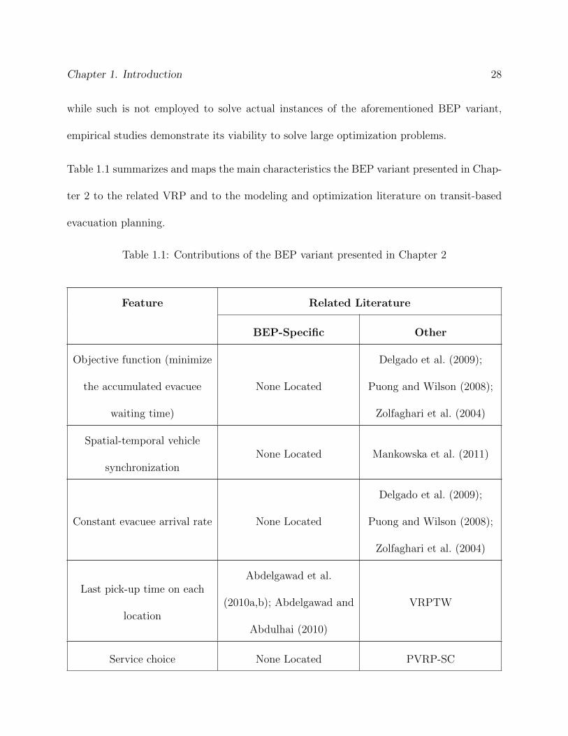
Table 1.1 summarizes and maps the main characteristics the BEP variant presented in Chap-
ter 2 to the related VRP and to the modeling and optimization literature on transit-based
evacuation planning.
Table 1.1: Contributions of the BEP variant presented in Chapter 2
Feature Related Literature
BEP-Specific Other
Objective function (minimize
the accumulated evacuee
waiting time)
None Located
Delgado et al. (2009);
Puong and Wilson (2008);
Zolfaghari et al. (2004)
Spatial-temporal vehicle
synchronizationNone Located Mankowska et al. (2011)
Constant evacuee arrival rate None Located
Delgado et al. (2009);
Puong and Wilson (2008);
Zolfaghari et al. (2004)
Last pick-up time on each
location
Abdelgawad et al.
(2010a,b); Abdelgawad and
Abdulhai (2010)
VRPTW
Service choice None Located PVRP-SC
Chapter 1. Introduction 29
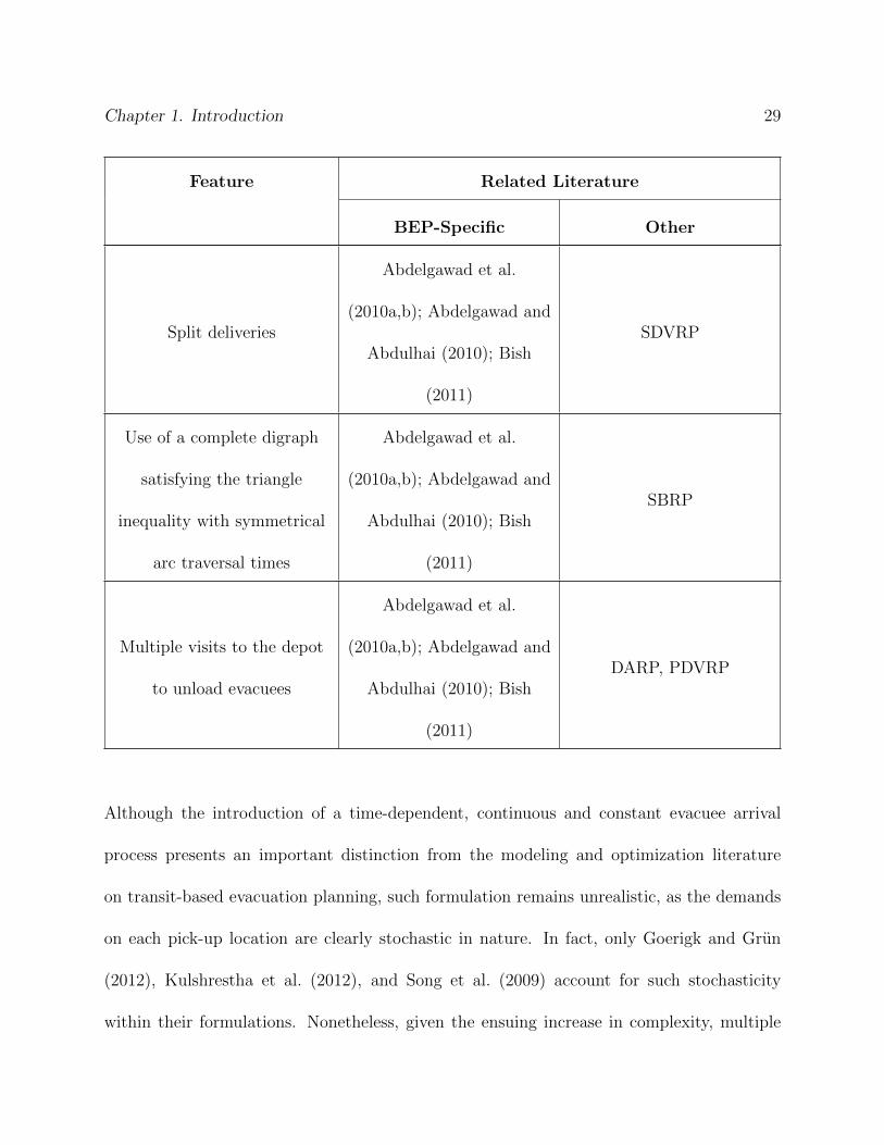
Feature Related Literature
BEP-Specific Other
Split deliveries
Abdelgawad et al.
(2010a,b); Abdelgawad and
Abdulhai (2010); Bish
(2011)
SDVRP
Use of a complete digraph
satisfying the triangle
inequality with symmetrical
arc traversal times
Abdelgawad et al.
(2010a,b); Abdelgawad and
Abdulhai (2010); Bish
(2011)
SBRP
Multiple visits to the depot
to unload evacuees
Abdelgawad et al.
(2010a,b); Abdelgawad and
Abdulhai (2010); Bish
(2011)
DARP, PDVRP
Although the introduction of a time-dependent, continuous and constant evacuee arrival
process presents an important distinction from the modeling and optimization literature
on transit-based evacuation planning, such formulation remains unrealistic, as the demands
on each pick-up location are clearly stochastic in nature. In fact, only Goerigk and Grun
(2012), Kulshrestha et al. (2012), and Song et al. (2009) account for such stochasticity
within their formulations. Nonetheless, given the ensuing increase in complexity, multiple
Chapter 1. Introduction 30
simplifying assumptions to improve the problem tractability are needed. Both Goerigk
and Grun (2012) and Kulshrestha et al. (2012) assume that the set of possible demands
(scenarios) are a known problem parameters, but, whereas Goerigk and Grun (2012) assume
that such scenarios have equally likely probability of realization, Kulshrestha et al. (2012)
assume that, at least, an arbitrary number of pick-up locations must attain their highest
demand scenario. Consequently, Kulshrestha et al. (2012), albeit indirectly, account for
the different likelihoods of each scenario over the optimal route and scheduling of the fleet.
Finally, Song et al. (2009) assume that evacuees arrive at the pick-up locations according to a
logistic distribution. The authors include a reliability constraint, introduced by Charnes and
Cooper (1963), within their formulation to ensure, under an arbitrary probability, that if the
given pick-up location is selected for the evacuation, then enough vehicles will arrive to meet
its demand. However, no justification was provided for the chosen distribution. Chapter 4
extends the BEP variant presented on Chapter 2 to account for the uncertainty on the number
of evacuees present at each pick-up location, and explores its effect over the expected total
travel time of the fleet. Nonetheless, in order to improve the problem tractability, similar to
Abdelgawad et al. (2010a,b); Abdelgawad and Abdulhai (2010); Bish (2011); Chen and Chou
(2009); Goerigk and Grun (2012); Goerigk et al. (2013); Kulshrestha et al. (2012); Margulis
et al. (2006); Song et al. (2009), and Wei and Zhaodong (2010), the formulation assumes that
all evacuees are at the pick-up locations at the onset of the evacuation; similar to Goerigk
and Grun (2012) and Kulshrestha et al. (2012), that the possible demands (scenarios) are
provided; and, similar to Goerigk and Grun (2012), that the demands are functions (possibly

Chapter 1. Introduction 31
multiples) of the bus capacities. The effect of uncertainty on the initial routing of vehicles is
explored. It is assumed that any uncertainty is resolved once buses visit the pick-up locations
for the first time.
Consequently, the proposed formulation can be classified as a two-stage stochastic D-VRP
with stochastic customers and demands, that is a D-VRP which relies on the known stochas-
tic nature of the demand in order to identify improved routes for the fleet, and which assumes
that some of the demands are potentially zero. Although the D-VRP literature is extensive,
its application to humanitarian logistics is somewhat scarce. In fact, no literature specifically
focusing on transit-based evacuation planning was located. Brotcorne et al. (2003) and Gen-
dreau et al. (2001) propose a D-VRP formulation for ambulance relocation during disaster
relief operations, whereas Haghani and Yang (2007) and Yi and Ozdamar (2007) propose
a D-VRP formulation for supply deployment during such operations. Finally, Fajardo and
Waller (2012) propose a D-VRP formulation for search-and-rescue operations. Although not
focused on transit-based evacuation planning, the authors introduce, perhaps, the closest
variant to the proposed problem formulation.
Fajardo and Waller (2012) introduce and analyze a single-vehicle, uncapacitated Stochastic
Dynamic Traveling Salesman Problem (Stochastic D-TSP) formulation for rescuing disaster
victims whose number and position is not known a priori. Their formulation shares several
commonalities with the BEP variant presented in Chapter 4. First, their formulation assumes
that a set of pick-up locations (i.e., a list of potential victim positions) and a set of potential
demands within each location are provided. Second, the realized demand on each location
Chapter 1. Introduction 32
(i.e., whether any victims are present or not) only becomes known upon visual observation,
that is, once vehicles visit the location for the first time. Consequently, the problem must be
re-optimized as additional information becomes available. Third, the authors also propose
a two-stage stochastic formulation, where, in the first stage, the subsequent arc traversal
for the vehicle is identified, and, in the second stage, the remaining arc traversals leading it
back to the depot under each possible location-scenario realization are identified. Finally,
their formulation also seeks to minimize the expected total travel time, provided a set of
scenario probabilities. Despite these similarities, their proposed formulation differs from the
variation presented in Chapter 4 is some important aspects. First, the authors modeled the
problem as a TSP. Consequently, efficiencies from using multiple vehicles and from allowing
vehicles to return to the depot to unload evacuees (or disaster victims) multiple times are
ignored. Second, their formulation focuses on a search-and-rescue operation rather than a
transit-based evacuation setting. Consequently, their formulation ignores vehicle capacity
restrictions, which are an important consideration of emergency evacuations. Finally, and
more importantly, while the authors mention the potential benefits of sampling and symme-
try, their formulation does not explicitly integrate these features in order to identify better
routes for the vehicle.
Lastly, some of the most commonly used VRP solution algorithms are presented.

Chapter 1. Introduction 33
1.4 Solution Methodologies
This section presents some of the most commonly used VRP solution algorithms. Although
such methodologies fall beyond the scope of this research, they are included here due to
their historical significance and due to their overt use within the modeling and optimization
literature on transit-based evacuation planning.
1.4.1 Exact Algorithms
1.4.1.1 The k-Degree Center Tree Algorithm
Christofides et al. (1981) propose an exact algorithm which relies on the properties of graphs
for solving symmetric (i.e., problems whose arc traversal cost is the same regardless if the
vehicle is traversing the arc from node i to node j or from node j to node i), single-depot
VRPs. The methodology is based on the m-TSP problem, that is, the problem of identi-
fying m routes for a single vehicle to visit all the nodes in the network. Figure 1.1 depicts
an example solution for a m-TSP with 2 routes over an undirected, complete graph. For
simplicity, the arc traversal costs are omitted.

Chapter 1. Introduction 34
0
1
2
3
5
6
4
Figure 1.1: An example optimum solution for a m-TSP with 2 routes.
In summary, the k-degree center tree algorithm identifies the routes that minimize the total
travel cost by building a spanning tree (i.e., a connected, acyclic subgraph spanning all nodes
in the original graph) rooted at the depot (in the example presented in Figure 1.1, node 0),
and, later, adding additional arcs between leafs and between leafs and the depot, such that
the final route has m cycles (tours). The algorithm derives its name from the fact that the
degree of the depot node, before the additional arcs are added, equals k. Consequently, the
algorithm partitions the set of network arcs, A, into four subsets:
• A0 : The subset of arcs not belonging to the optimum solution;
• A1 : The subset of arcs forming a k-degree center tree, that is, a spanning tree where
the degree of the depot node, k, equals 2m− y;
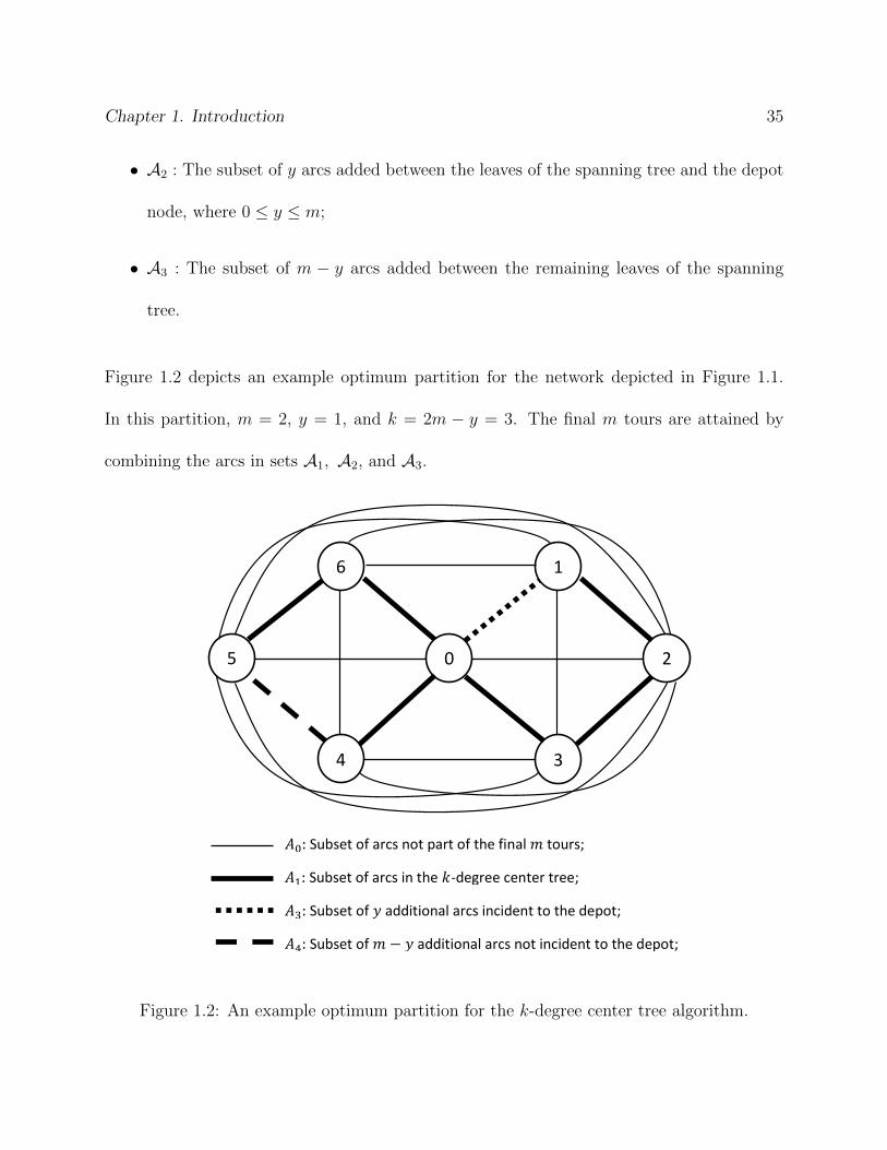
Chapter 1. Introduction 35
• A2 : The subset of y arcs added between the leaves of the spanning tree and the depot
node, where 0 ≤ y ≤ m;
• A3 : The subset of m − y arcs added between the remaining leaves of the spanning
tree.
Figure 1.2 depicts an example optimum partition for the network depicted in Figure 1.1.
In this partition, m = 2, y = 1, and k = 2m − y = 3. The final m tours are attained by
combining the arcs in sets A1, A2, and A3.
0
1
2
3
5
6
4
Subset of arcs not part of the final tours;
Subset of arcs in the -degree center tree;
Subset of additional arcs incident to the depot;
Subset of additional arcs not incident to the depot;
Figure 1.2: An example optimum partition for the k-degree center tree algorithm.

Chapter 1. Introduction 36
Now, let xta be a binary decision variable that equals one if arc a belongs to partition
At, t ∈ {1, 2, 3}, and equals zero otherwise. Moreover, let y ∈ {y ∈ Z|0 ≤ y ≤ m}, such
that the problem to minimize the total travel cost can be formulated as follows:
Minimize∑
a∈A
ca(x1a + x2
a + x3a) (1.1)
Subject to∑
a∈(S,S)
x1a ≥ 1, ∀ S ⊆ N , |S| ≥ 1 (1.2)
∑
a∈A1
x1a = 2m− y (1.3)
∑
a∈A
x1a = |N | − 1 (1.4)
∑
a∈A1
x2a = y (1.5)
∑
a∈A\A1
x3a = m− y (1.6)
∑
a∈Ai
(x1a + x2
a + x3a) = 2, i = 2, · · · , |N |. (1.7)
Objective Function (1.1) minimizes the total cost of the arcs included in the final solution.
Constraints (1.2)-(1.4) build the k-degree center tree. Constraint (1.2) prevents the inclusion
of arcs leading to cycles in the spanning tree, (1.3) forces the degree of the depot, k, to equal
2m− y, and (1.4) ensures that the resulting tree spans all nodes in the network. Constraint
(1.5) forces the inclusion of y additional arcs connecting the leaves of the spanning tree
back to the depot, and (1.6) forces the inclusion of m − y additional arcs connecting the
remaining leaves of the spanning tree. Finally, (1.7) forces the degree of every node (except
the depot’s) to equal 2. This constraint is similar to the flow conservation constraint in
traditional TSP formulations. Next, Constraint (1.7) is relaxed via Lagrangian relaxation,
Chapter 1. Introduction 37
and (1.1) becomes:
Minimize∑
a∈A
ca(x1a + x2
a + x3a) +
∑
a∈A
(λα(a) + λβ(a))(x1a + x2
a + x3a)− 2
|N |∑
i=2
λi
⇒ Minimize3∑
t=1
∑
a∈A
(ca + λα(a) + λβ(a))xta − 2
|N |∑
i=2
λi,
Where, λ denotes the Lagrangean multiplier vector, and α(a) and β(a) denote the nodes
adjoined by arc a ∈ A. Consequently, given an arbitrary y-value, the resulting problem can
be decomposed into three subproblems, one for each subset of A except A0, and each with
Objective Function:
Minimize∑
a∈A
(ca + λα(a) + λβ(a))xta, ∀ t ∈ {1, 2, 3}. (1.8)
Although these subproblems can be solved relatively quickly, they only return a lower bound
on the objective function value for the original problem. Nonetheless, such lower bound
can be used as a fathoming criterion during the ensuing branch and bound algorithm, thus
reducing the overall computation time of the problem. Despite its improved performance and
its historical significance, the k-degree center tree algorithm can only be used for symmetric,
single-depot VRPs, and, thus, is not sufficiently robust for the wide array of VRP variations
used within the modeling and optimization literature on transit-based evacuation planning.
1.4.1.2 Set Partitioning and Column Generation
The column generation algorithm was introduced by Dantzig and Wolfe (1960), but it was
first applied to VRPs by Balinski and Quandt (1964). Consider the following VRP formula-

Chapter 1. Introduction 38
tion:
Let zij be a binary parameter that equals one if node i ∈ N is part of route j ∈ J (where N
is the set of all nodes in the network and J is the set of all possible cycles that include the
depot), let cj be the total cost of route j, and, finally, let xj be a binary decision variable
that equals 1 if route j ∈ J is selected.
The problem can be formulated as follows:
Minimize∑
j∈J
cjxj (1.9)
Subject to∑
j∈J
zijxj = 1, ∀ i ∈ N\{0}, (1.10)
Where, Objective Function (1.9) identifies the subset of routes from set J that incur the
lowest cost, and Constraint (1.10) ensures that these routes serve each customer exactly
once. Here, node 0 is the depot. The formulation holds from the fact that set J is finite,
as any network with a finite number of nodes has a finite number of paths connecting these
nodes.
Unfortunately, since the number of possible routes in set J grows exponentially with the
number of customers, the ensuing problem may require a considerably long time to solve. In
addition, it may be difficult to determine the feasibility of the route in capacitated VRPs,
a particularly cumbersome problem when split deliveries are allowed. Nonetheless, the issue
can be addressed by column generation.
In summary, the column generation algorithm decomposes the original problem into a relaxed

Chapter 1. Introduction 39
master problem, containing only a subset of the decision variables, and a subproblem. First,
the relaxed master problem identifies the optimum dual vector, and, once such vector has
been identified, a subproblem aiming to identify the corresponding entering variable, xs,
with minimum marginal cost (based on the identified dual vector) is generated and solved.
If the objective function value of the subproblem is non-positive (i.e., if the marginal cost
of every potential entering variable does not improve the objective function value of the
master problem), then the solution is optimum. Otherwise, another iteration is performed.
Since only a subset of potential variables is assessed on each iteration of the algorithm,
the computation time is considerably reduced. See Bazaraa et al. (2005, p. 333-364) for a
detailed description of the algorithm and for numerical examples.
Wilhelm (2001) reviews the use of the column generation algorithm for solving integer pro-
gramming problems, including the VRPTW. According to the author, despite the reduced
computation time, several issues remain. First, since the algorithm is based on the Revised
Simplex algorithm (except for the identification of the entering column, which is performed
within the subproblem, and, thus, can rely on a different solution methodology), it suffers
from its the same disadvantages, foremost of which are the precision issues ensuing from the
matrix inversion step. Second, the presence of degenerate constraints may lead to cycling or
even stalling. Finally, current solution strategies may require a large number of subproblems
to be solved for each entering column.
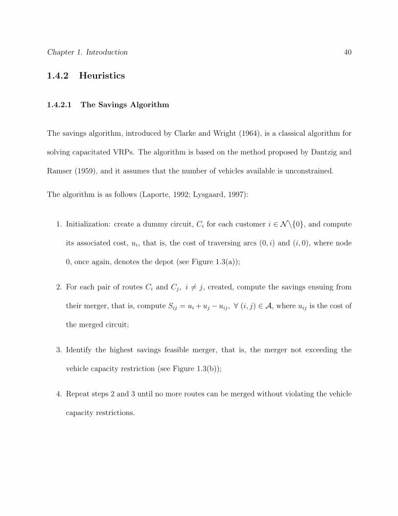
Chapter 1. Introduction 40
1.4.2 Heuristics
1.4.2.1 The Savings Algorithm
The savings algorithm, introduced by Clarke and Wright (1964), is a classical algorithm for
solving capacitated VRPs. The algorithm is based on the method proposed by Dantzig and
Ramser (1959), and it assumes that the number of vehicles available is unconstrained.
The algorithm is as follows (Laporte, 1992; Lysgaard, 1997):
1. Initialization: create a dummy circuit, Ci for each customer i ∈ N\{0}, and compute
its associated cost, ui, that is, the cost of traversing arcs (0, i) and (i, 0), where node
0, once again, denotes the depot (see Figure 1.3(a));
2. For each pair of routes Ci and Cj, i 6= j, created, compute the savings ensuing from
their merger, that is, compute Sij = ui + uj − uij, ∀ (i, j) ∈ A, where uij is the cost of
the merged circuit;
3. Identify the highest savings feasible merger, that is, the merger not exceeding the
vehicle capacity restriction (see Figure 1.3(b));
4. Repeat steps 2 and 3 until no more routes can be merged without violating the vehicle
capacity restrictions.
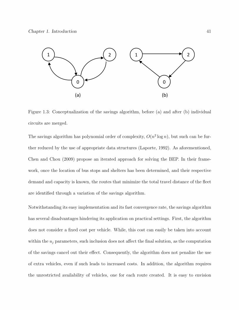
Chapter 1. Introduction 41
1 2
0
1 2
(a)
0
(b)
Figure 1.3: Conceptualization of the savings algorithm, before (a) and after (b) individual
circuits are merged.
The savings algorithm has polynomial order of complexity, O(n2 log n), but such can be fur-
ther reduced by the use of appropriate data structures (Laporte, 1992). As aforementioned,
Chen and Chou (2009) propose an iterated approach for solving the BEP. In their frame-
work, once the location of bus stops and shelters has been determined, and their respective
demand and capacity is known, the routes that minimize the total travel distance of the fleet
are identified through a variation of the savings algorithm.
Notwithstanding its easy implementation and its fast convergence rate, the savings algorithm
has several disadvantages hindering its application on practical settings. First, the algorithm
does not consider a fixed cost per vehicle. While, this cost can easily be taken into account
within the uj parameters, such inclusion does not affect the final solution, as the computation
of the savings cancel out their effect. Consequently, the algorithm does not penalize the use
of extra vehicles, even if such leads to increased costs. In addition, the algorithm requires
the unrestricted availability of vehicles, one for each route created. It is easy to envision
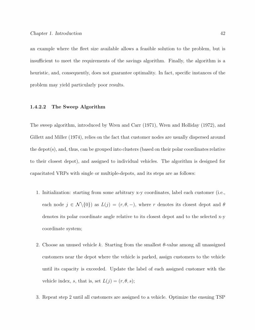
Chapter 1. Introduction 42
an example where the fleet size available allows a feasible solution to the problem, but is
insufficient to meet the requirements of the savings algorithm. Finally, the algorithm is a
heuristic, and, consequently, does not guarantee optimality. In fact, specific instances of the
problem may yield particularly poor results.
1.4.2.2 The Sweep Algorithm
The sweep algorithm, introduced by Wren and Carr (1971), Wren and Holliday (1972), and
Gillett and Miller (1974), relies on the fact that customer nodes are usually dispersed around
the depot(s), and, thus, can be grouped into clusters (based on their polar coordinates relative
to their closest depot), and assigned to individual vehicles. The algorithm is designed for
capacitated VRPs with single or multiple-depots, and its steps are as follows:
1. Initialization: starting from some arbitrary x-y coordinates, label each customer (i.e.,
each node j ∈ N\{0}) as L(j) = (r, θ,−), where r denotes its closest depot and θ
denotes its polar coordinate angle relative to its closest depot and to the selected x-y
coordinate system;
2. Choose an unused vehicle k. Starting from the smallest θ-value among all unassigned
customers near the depot where the vehicle is parked, assign customers to the vehicle
until its capacity is exceeded. Update the label of each assigned customer with the
vehicle index, s, that is, set L(j) = (r, θ, s);
3. Repeat step 2 until all customers are assigned to a vehicle. Optimize the ensuing TSP
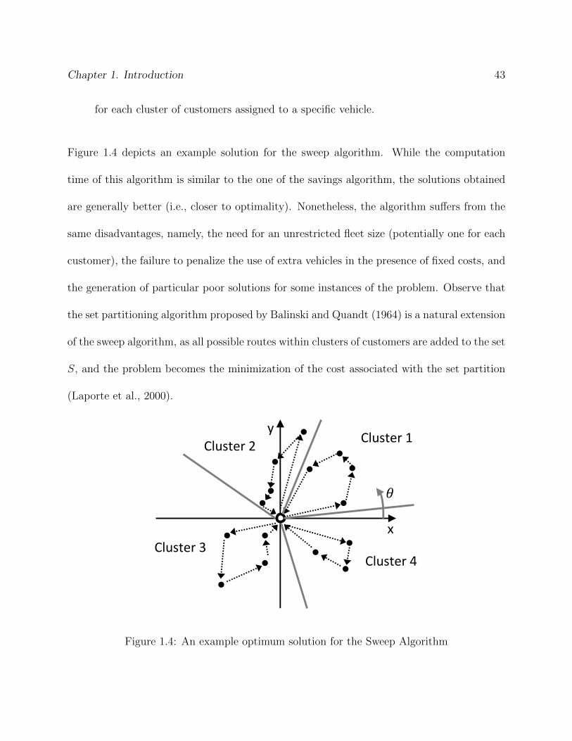
Chapter 1. Introduction 43
for each cluster of customers assigned to a specific vehicle.
Figure 1.4 depicts an example solution for the sweep algorithm. While the computation
time of this algorithm is similar to the one of the savings algorithm, the solutions obtained
are generally better (i.e., closer to optimality). Nonetheless, the algorithm suffers from the
same disadvantages, namely, the need for an unrestricted fleet size (potentially one for each
customer), the failure to penalize the use of extra vehicles in the presence of fixed costs, and
the generation of particular poor solutions for some instances of the problem. Observe that
the set partitioning algorithm proposed by Balinski and Quandt (1964) is a natural extension
of the sweep algorithm, as all possible routes within clusters of customers are added to the set
S, and the problem becomes the minimization of the cost associated with the set partition
(Laporte et al., 2000).
Cluster 1 Cluster 2
Cluster 3 Cluster 4
y
x
Figure 1.4: An example optimum solution for the Sweep Algorithm

Chapter 1. Introduction 44
1.4.3 Metaheuristics
1.4.3.1 Simulated Annealing
In the physical annealing process, a solid (such as a metal) is melted and its temperature
is then slowly lowered to the vicinity of its freezing point, allowing its atoms to form a
crystalline pattern (Aarts et al., 1997; Kirkpatrick et al., 1983). Metropolis et al. (1953)
present an analytical, iterative algorithm to search for the thermal equilibrium of the system.
In each step of the algorithm, the displacement of an atom is simulated and the resulting
energy of the material is computed using tools from statistical mechanics. If the resulting
change in energy of the material is non-positive (i.e., if the atom displacement led to cooling
of the material), then the change is accepted. Conversely, if the change in energy of the
material is strictly positive, then it may be accepted with an arbitrary probability. The new
configuration is then used as the starting point for the next iteration. Since the algorithm
allows intermediary configurations to have higher energies, it is less likely to converge to a
local optimal solution.
The first use of the algorithm for identifying good solutions to combinatorial optimization
problems can be attributed to Kirkpatrick et al. (1983). The authors extend the Metropolis
et al. (1953) algorithm to account for annealing schedules, where the equilibrium ”tempera-
ture” of the material is updated between runs of the Metropolis algorithm via an exponential
curve that simulates its gradual cooling. Brooks and Morgan (1995) presents the following
summary of the Simulation Annealing algorithm for optimization problems:

Chapter 1. Introduction 45
1. Initialization:
• Set k = 0 and identify an initial feasible solution, x0, either generated randomly
or through another heuristic;
• Compute the objective function value, E(x0), corresponding to x0;
• Arbitrarily select an initial, and potentially high, temperature, T0, and a constant,
u, sampled from an Uniform(0,1) distribution;
2. Identify the equilibrium solution for the current temperature, T :
• Update the iteration number, that is, set k = k + 1;
• Randomly identify an alternative solution, xk, within an arbitrary neighborhood
of the previous feasible solution (e.g., in a TSP, this step may consist of switching
the order in which two nearby nodes are visited);
• Compute the objective function value, E(xk), corresponding to xk;
• If E(xk) ≤ E(xk−1)− T lnu, then set xk as the new solution;
• Repeat this step until a certain criteria is met (e.g., E(xk−1) − E(xk) < ε for a
certain number of iterations). The system is now in equilibrium with the temper-
ature T ;
3. Perform an annealing schedule, that is, after the equilibrium solution is identified,
update the temperature by setting T = knT0, where k is a constant between 0 and 1,
exclusively, and n is the number of annealing schedules previously performed. Identify
the equilibrium solution for the new temperature;

Chapter 1. Introduction 46
4. Repeat the annealing schedule step until a certain criteria is met (e.g., E(xn−1) −
E(xn) < ε for a certain number of iterations). After the termination criteria has been
met, the system is considered frozen.
The simulated annealing algorithm has been applied to a variety of settings and has shown
ambivalent performance depending on the problem characteristics (Aarts et al., 1997). Sev-
eral variations have been proposed to improve its performance (speed and convergence rate).
These, however, are beyond the scope of this research. In the modified genetic algorithm
proposed by Deai et al. (2011) to solve the BEP, simulated annealing is used to determine
the selection probability of each chromosome.
1.4.3.2 Genetic Approaches
Genetic approaches, a subclass of evolutionary algorithms, are random searches inspired by
the Darwinian evolutionary process (Larranaga et al., 1999). In these algorithms, solutions
for the optimization problem (not necessarily feasible solutions) are represented by strings,
referred to as chromosomes. For instance, the solution x1 = 0, x2 = 1, and x3 = 1 can
be represented by the string ”011.” The algorithm simulates the evolution of this artificial
population over time until a good string is produced. The term Genetic Algorithm can be
attributed to Holland (1975), who consolidated the existing ideas of the time (namely the
use of mutation associated with hill-climbing methods) and further developed the algorithm
to accommodate recombination of selected individuals (Reeves, 2003). In summary, the
algorithm is as follows (modified from Larranaga et al., 1999, page 131, and Reeves, 2003,
Chapter 1. Introduction 47
page 59):
1. Initialization: Randomly generate a population of chromosomes.
2. Produce a new generation of chromosomes:
(a) Select parents from the current population and produce children from these indi-
viduals via crossover ;
(b) Mutate these individuals;
(c) Evaluate the fitness of the new generation of chromosomes (parents and offspring)
and destroy unfit ones;
3. Repeat Step 2 until a certain termination criteria is satisfied (e.g, until a certain number
of generations has been produced or no significant changes in the objective function
value from the best chromosome has been observed in a certain number of generations).
Crossover is the process in which parent chromosomes are randomly combined to generate
new offspring. Figure 1.5 exemplifies the crossover of two parent strings (P1 and P2) to
generate two offspring (O1 and O2).
P1: 1 0 1 0 0 1 0
P2: 0 1 1 1 0 0 1
O1: 1 0 1 1 0 0 1
O2: 0 0 1 0 0 1 1
Figure 1.5: An example of crossover under the Genetic Algorithm.
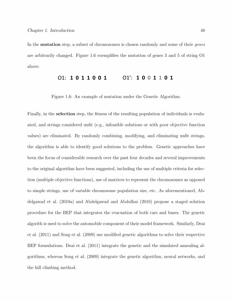
Chapter 1. Introduction 48
In the mutation step, a subset of chromosomes is chosen randomly and some of their genes
are arbitrarily changed. Figure 1.6 exemplifies the mutation of genes 3 and 5 of string O1
above.
O1: 1 0 1 1 0 0 1 O1’: 1 0 0 1 1 0 1
Figure 1.6: An example of mutation under the Genetic Algorithm.
Finally, in the selection step, the fitness of the resulting population of individuals is evalu-
ated, and strings considered unfit (e.g., infeasible solutions or with poor objective function
values) are eliminated. By randomly combining, modifying, and eliminating unfit strings,
the algorithm is able to identify good solutions to the problem. Genetic approaches have
been the focus of considerable research over the past four decades and several improvements
to the original algorithm have been suggested, including the use of multiple criteria for selec-
tion (multiple objective functions), use of matrices to represent the chromosomes as opposed
to simple strings, use of variable chromosome population size, etc. As aforementioned, Ab-
delgawad et al. (2010a) and Abdelgawad and Abdulhai (2010) propose a staged solution
procedure for the BEP that integrates the evacuation of both cars and buses. The genetic
algorith is used to solve the automobile component of their model framework. Similarly, Deai
et al. (2011) and Song et al. (2009) use modified genetic algorithms to solve their respective
BEP formulations. Deai et al. (2011) integrate the genetic and the simulated annealing al-
gorithms, whereas Song et al. (2009) integrate the genetic algorithm, neural networks, and
the hill climbing method.

Chapter 1. Introduction 49
1.4.3.3 Tabu Search
The origins of the tabu search algorithm can be traced to Glover (1977), which used some
of its elements to generate surrogate constraints for integer programming problems (i.e.,
inequalities implied by one or more constraints that eliminate non-integer portions of the
feasible region). The algorithm, formalized by Glover (1986), starts by identifying an initial
solution, x1, and then, on each iteration, proceeding towards an improving direction until
a certain criteria is satisfied, such as a maximum number of iterations has been reached or
the problem has shown no improvement for several iterations (Laporte et al., 2000). Since
successive solutions not necessarily have smaller objective function values, solutions that
were recently examined are disallowed (or tabued) in order to prevent cycling (Glover, 1986).
It is also important to note that intermediate solutions may not be feasible (Laporte, 1992).
The tabu search algorithm is readily applicable to a variety of settings. The following varia-
tion (modified from Laporte, 1992, page 356) seeks good solutions for the VRP. Throughout,
let T denote the tabu list, Rr denote the subset of customer nodes visited by route r, such
that each node belongs to exactly one route, x denote current solution set (i.e., the current
set of routes R1, · · · , Rm found), and Np(x) denote the set of nearby solutions around x
(obtained, for instance, by switching the nodes visited between two routes). The algorithm
is as follows:
1. Create circuits connecting the depot and each customer (i.e., let route j consist of arcs
(0, j)∪ (j, 0), ∀ j ∈ N\{0}) regardless if these routes are feasible or not. Let x denote
Chapter 1. Introduction 50
such solution, and let F (x) denote its associated objective function value, that is, let
F (x) =∑
r
∑(i,j)∈Rr
cij. Set T = ∅;
2. Let Np(x) denote the set of all solutions in a neighborhood of radius p from the current
solution x. If Np(x)\T = ∅, then go to step 3: all nearby solutions are tabued.
Otherwise identify the least cost solution, y ∈ Np(x)\T , and set x = y (i.e., update
the best known solution);
3. If the stopping criteria has been met (e.g., if a maximum number of iterations has
been reached or no significant improvement in the objective function value have been
observed for a certain number of iterations), stop. Otherwise set T = T ∪ {x} and
return to step 2.
According to Basu and Ghosh (2008), tabu search is widely used to solve practical combi-
natorial optimization problems. In addition, Gendreau et al. (1994) propose a modification
which prevents the insertion of nodes far from the current solution and forces an assessment
of variations of the final solution, thus improving the convergence rate and the quality of
the final solution. As aforementioned, Abdelgawad et al. (2010b) propose solving their BEP
formulation via constraint programming, where multiple search strategies - including the
Tabu search metaheuristic - and constraint propagation techniques are used to obtain good,
feasible solutions to the problem. In addition, one of the heuristics for solving the BEP
proposed by Bish (2011) involves route swapping and reassignment, elements of the tabu
search metaheuristic. Finally, Goerigk and Grun (2012) and Sayyady and Eksioglu (2010)
Chapter 1. Introduction 51
use the tabu search metaheuristic to solve their respective BEP formulations.
1.4.3.4 Ant Colony Optimization
As the name suggests, the ant colony optimization algorithm, introduced by Colorni et al.
(1991), simulates the decision making process of ants as they find the most efficient trail
from their nest to every available food source and back. In nature, ants deposit pheromones
as they travel along a trail. The larger the amount of pheromone in a trail, the higher the
probability that other ants will follow it, and, if they do, their own pheromone reinforces
the existing trail. Since shorter, more direct routes are traversed more often, the amount
of pheromones on these trails are more quickly reinforced, whereas the one in less direct
routes slowly evaporates, becoming less likely to be followed by other ants. Nonetheless,
the continuous random selection of trails by individual ants helps the colony to discover
more efficient routes (Bell and McMullen, 2004). The algorithm was initially developed for
identifying good solutions to the TSP, but it has since been modified and applied to a variety
of other problems, including several variations of the VRP.
In the original algorithm, each of the n nodes (food sources and nest) has |bi(k)|, i = 1, · · · , n,
ants, such that the total number of ants, m, equals∑n
i=1 |bi(k)|. As each ant starts its tour,
the intensity of pheromone on arc (i, j) ∈ A at iteration k, τij(k), is updated as follows:
τij(k) = ρ · τij(k − 1) + ∆τij(k − 1, k), (1.11)
Where ρ is an arbitrary pheromone evaporation coefficient and ∆τij(k− 1, k) is the amount
Chapter 1. Introduction 52
of pheromone deposited on arc (i, j) between iterations k − 1 and k. Colorni et al. (1991)
suggests that, if ant y traverses arc (i, j), then the amount of pheromone it deposits can either
be a fixed, arbitrary quantity, Q, or a function of the travel distance between nodes i and j
(e.g., ∆τij(k−1, k) = Q/cij). The initial pheromone intensity on each path, τij(0), ∀ (i, j) ∈
A, can be chosen arbitrarily. Given the current amount of pheromone on each path, the
desirability of node j starting from node i at iteration k, pij(k), is computed as follows:
pij(k) =(τij(k))α/(cij)
β
∑s:(i,s)∈A(τis(k))α/(tis)β
, (1.12)
Where the arbitrary parameters α and β control the relative importance of selecting shorter
travel distances versus highly traveled ones (i.e., paths with high pheromone intensities). In
order to prevent subtours, a tabu list is associated with each ant such that visits to repeated
food sources is disallowed. In summary, the algorithm is as follows (modified from Colorni
et al., 1991, page 5):
1. Initialization:
• Set T = ∞, T y = 0, ∀ y = 1, · · · ,m, k = 1, ∆τij(0, 1) = 0, ∀ (i, j) ∈ A, and
Ly = ∅, ∀ y = 1, · · · ,m (Ly is the tabu list associated with ant y);
• Choose the parameters: τij(0), ∀ (i, j) ∈ A, α, β, and bi(0), ∀ i = 1, · · · , n, the
last one satisfying∑n
i=1 |bi(0)| = m;
2. For every node i = 1, · · · , n and for every ant y ∈ bi(k):
(a) For every j 6∈ Ly, compute pij(k) ∀ j : (i, j) ∈ A via Equation (1.12); set pij(k) = 0
otherwise. Set j = arg max pij(k);
Chapter 1. Introduction 53
(b) Set ∆τij(k − 1, k) = ∆τij(k − 1, k) + f(Q), where f(Q) = Q or f(Q) = Q/cij, as
aforementioned;
(c) Update τij(k) via Equation (1.11), set Ly = Ly ∪ {j}, and set T y = T y + cij;
3. Repeat step 2 until Ly, ∀ y = 1, · · · ,m includes every node in the network. Save
the best solution found (i.e., set T = min{T,miny=1,··· ,m Ty}) and erase the tabu lists.
Repeat for an arbitrary number of iterations.
Observe that the described implementation of the algorithm does not constitute a random
search, as paths are selected deterministically. A random search, however, can be easily
implemented by using the inverse CDF method to sample a path from the desirabilities not
in the tabu list. The ant colony optimization algorithm initially yielded poor results when
applied to VRPs. However, several modifications have been proposed since its introduction.
According to (Bell and McMullen, 2004), such modifications have led to solutions within 1%
of the known optimum for small VRP variations.
1.4.4 Summary of Solution Algorithms
This section introduced different algorithms that rely on the known structure of VRPs to
reduce its computation time. Unfortunately, to date, none of these methods is capable or
solving particularly large VRP instances (i.e., instances with many vehicles and customers)
to optimality.
The k-degree center tree algorithm, introduced by Christofides et al. (1981), and the column
Chapter 1. Introduction 54
generation algorithm, introduced by Dantzig and Wolfe (1960), are presented as examples
of exact optimization methods. These methods always identify the optimum solution to the
problem, but, since they require the concomitant use of the branch and bound algorithm,
they may take a particularly long time to solve. The k-degree center tree algorithm relies
on the known properties of graphs to build a spanning tree rooted at the depot, and, later,
identifies the set of additional arcs needed to generate a predetermined number of tours for
the fleet. Conversely, Balinski and Quandt (1964) reason that any graph with a finite number
of customers has a finite number of potential routes serving these customers. However,
instead of enumerating every possibility, the problem can be solved by column generation,
that is, by assessing the benefits of one route at a time.
The savings algorithm, introduced by Clarke and Wright (1964), and the sweep algorithm,
whose origins can be traced to Wren and Carr (1971), Wren and Holliday (1972), and Gillett
and Miller (1974), are presented as examples of heuristics. These algorithms are easy to
implement and have fast convergence rate. However, they may also yield particularly poor
results depending on the problem instance. The savings algorithm relies on the idea of
consolidating existing routes by appending connecting arcs and removing redundant ones.
The sweep algorithm uses the fact that customer nodes are usually dispersed around the
depot, and, thus, can be grouped into clusters (based on their polar coordinates relative to
their closest depot and to an arbitrary x-y coordinate system), and assigned to individual
vehicles. In summary, the algorithm transforms the VRP into a m-TSP, a much more efficient
formulation.
Chapter 1. Introduction 55
Finally, the simulated annealing, introduced by Metropolis et al. (1953) and first applied
to combinatorial optimization problems by Kirkpatrick et al. (1983), the genetic algorithm,
whose origin can be attributed to Holland (1975), the tabu search algorithm, introduced
by Glover (1986), and the ant colony optimization algorithm, introduced by Colorni et al.
(1991), are presented as examples of metaheuristics. Since these methods do not require the
simultaneous use of the branch and bound algorithm, they are particularly suited to com-
binatorial optimization problems. As the name suggests, the simulated annealing algorithm
simulates the physical annealing process using tools from statistical mechanics. The genetic
algorithm, a subclass of evolutionary algorithms, is a random search method inspired by
the Darwinian evolutionary process of crossover, mutation, and selection. The tabu search
algorithm searches for nodes to be included or excluded from the route that lead to im-
provements in the objective function value without ever returning to a previous solution.
Finally, the ant colony optimization algorithm, a particle swarm metaheuristic, simulates
the decision process of ants (vehicles) traveling on a set of trails (arcs) in search for food
sources (customers).

Chapter 2
Scheduling and Routing for a
Bus-based Evacuation with Constant
Evacuee Arrival Rate
56
Chapter 2. Sch. and Routing for a Bus-based Evac. with Const. Evacuee Arrival Rate 57
Scheduling and Routing for a Bus-based Evacuation
with Constant Evacuee Arrival Rate
Victor C. Pereira and Douglas R. Bish
(ABSTRACT)
This paper introduces a variant of the vehicle routing problem adapted for bus-based, re-
gional evacuation planning, where evacuees arrive at predetermined pick-up locations at
constant, location-specific rates. This arrival process more realistically portrays evacuee
arrival behavior, presenting an important distinction from the current transit-based evacua-
tion literature. In this problem, capacitated buses are routed, potentially multiple times, to
transport all evacuees to a depot/shelter such that the last pick-up, and the end of the arrival
process, occurs at a location-specific time, determined by risk considerations. The problem
seeks to minimize waiting time at these locations (total exposure) and exploits efficiencies
from allowing service choice. The structural properties of this problem guide the choice
for two important strategic parameters: the maximum number of pick-ups allowed on each
location and the fleet size. It is shown that, depending on the problem instance, increasing
the maximum number of pick-ups may reduce both the fleet size requirement and the total
exposure, and that, past a certain threshold, there exists a maximum number of pick-ups (or
a range of potential values, if the problem cannot be solved to optimality) that guarantees
an efficient usage of the available fleet and equitable reductions in exposure across pick-up
locations.
Chapter 2. Sch. and Routing for a Bus-based Evac. with Const. Evacuee Arrival Rate 58
Keywords: Evacuation planning; bus scheduling; vehicle routing problem; mixed-integer
programming
Acknowledgments: This work has been supported by the National Science Foundation
under Award Numbers 0825611 and 1055360. The authors would also like to thank Dr.
Barbara Fraticelli, the two anonymous referees, and the associate editor of Transportation
Science for their valuable insights.
2.1 Introduction
Most of the planning emphasis for large-scale, regional evacuations is automobile-centric.
While such planning is extremely important, there can be a large segment of the popu-
lation without access to automobiles, and, consequently, without the means to leave the
disaster area. For instance, it is estimated that between 200,000 and 300,000 residents of
New Orleans did not have access to any reliable means of personal transportation prior to
Hurricane Katrina’s landfall in 2005 (Wolshon, 2002), and that between 100,000 and 120,000
people remained in the city, under unsafe conditions, after the evacuation (Nigg et al., 2006).
According to Litman (2006), while the 500 buses available at the time were insufficient to
evacuate all transit-dependent residents of New Orleans in a single trip, they would have
sufficed, given the 48 hours of advanced notice, were it not for a lack of planning. Clearly,
the development of safe and efficient, bus-based, regional evacuation plans is an important
part of disaster preparedness.
Chapter 2. Sch. and Routing for a Bus-based Evac. with Const. Evacuee Arrival Rate 59
This paper introduces, formulates, and analyzes the Bus Evacuation Problem with Constant
Evacuee Arrival Rate (BEP-CA), a variant of the vehicle routing problem (VRP) adapted
for bus-based, regional evacuation planning. In this problem, evacuees gather at the pick-up
locations at constant rates, from the start of the evacuation to a location-specific end-time
(dictated by risk considerations). The BEP-CA seeks a pick-up schedule at these locations
and the corresponding routes for a fleet of buses in such a way that the total exposure is
minimized (i.e., that the total evacuee waiting time at these locations is minimized). At each
scheduled pick-up time, all evacuees present must be served and eventually transported to
a depot/shelter. The formulation forces at least one pick-up to take place at each pick-up
location, scheduled for the time when the arrival process of evacuees ends. Efficiencies from
allowing buses to unload evacuees at the depot multiple times and from service choice, that
is, from selecting the optimal number of pick-ups at each location (up to a maximum service
level), are exploited.
The modeling research on bus-based evacuations is somewhat limited. Abdelgawad et al.
(2010a,b) and Abdelgawad and Abdulhai (2010) investigate the effect of different objec-
tive functions on a multi-modal (automobile and mass transit) evacuation problem. Bish
(2011) proposes and analyzes two alternative models for the multi-depot, multi-trip, bus-
based evacuation problem: the first simultaneously identifies optimal route construction and
assignment, while the second identifies the optimal route assignment from a set of feasi-
ble routes. Chen and Chou (2009) propose a model that determines pick-up and shelter
locations that minimize infrastructure development cost, and, then, the optimal routes for
Chapter 2. Sch. and Routing for a Bus-based Evac. with Const. Evacuee Arrival Rate 60
the evacuation of transit-dependent students of a university campus. Simulation is used to
study the effect of vehicular contraflow on the results obtained. Deai et al. (2011) propose
a VRP with time windows, such that, for each time window, a certain number of buses are
available, a certain number of evacuees are at each pick-up location, and every location with
non-zero demand must be served by exactly one vehicle. Goerigk and Grun (2012) propose a
deterministic and a stochastic formulation without recourse in which vehicles perform round
trips between pick-up locations and shelters until each location is visited a certain number
of times. The stochastic formulation balances the number of buses that depart immediately
with those that remain stationed at the depot waiting for the demand at each location to
become known. Kulshrestha et al. (2012) propose and analyze a stochastic model without
recourse that selects which pick-up locations to open and the corresponding routes for a fleet
of buses such that their total travel time is minimized. Vehicles are initially assigned to
one of the possible pick-up locations, and, from there, they perform round trips to a set of
capacitated shelters until either all demand is satisfied or they reach a limiting travel time.
The formulation assumes that a set of scenarios is provided, but it limits the number of
pick-up locations whose demand can differ from the expected value. Sayyady and Eksioglu
(2010) propose a model for the single-depot evacuation problem, which incorporates traffic
flow dynamics from a simulation package and a logistic function to estimate the number
of evacuees at each pick-up location. Song et al. (2009) propose a stochastic model, which
selects optimal shelters from a set of candidate nodes and which accounts for the uncertainty
on the number of transit-dependent evacuees at each pick-up location by introducing a re-
Chapter 2. Sch. and Routing for a Bus-based Evac. with Const. Evacuee Arrival Rate 61
liability constraint. The model incorporates strict pick-up time windows, but assumes that
all evacuees are at the pick-up locations at time zero. Wei and Zhaodong (2010) propose
a model for solving the multi-modal (cars and buses) evacuation problem. Finally, Zheng
(2013) proposes a formulation which, similar to Goerigk and Grun (2012), models demand
in terms of the number of pick-ups required on each location, and which, similar to Deai
et al. (2011) and Song et al. (2009), enforces strict pick-up time windows.
The BEP-CA has several characteristics that distinguish it from the related evacuation plan-
ning and VRP literature. First, the literature almost invariably assumes that all demand is
ready, whereas the BEP-CA assumes that demand accumulates over time and under con-
stant, location-specific rates. Deai et al. (2011) and Zheng (2013) incorporate time-dependent
evacuee demand through the use of time windows, but such approach still assumes that de-
mand is ready and static within each time window. More importantly, since time windows
disassociate the routing and scheduling decisions, they may lead to infeasibility or to subop-
timal solutions. Although not in a VRP setting, such a linear arrival process has been used
to model transportation problems. For instance, Delgado et al. (2009) propose a model to
identify the pick-up schedule for a fleet of buses traversing a transit corridor that minimizes
passenger waiting and travel time; Puong and Wilson (2008) propose a model for urban
rail transit lines that allows trains to wait at designated stations following a disruption in
service; and Zolfaghari et al. (2004) propose a model that uses real-time information to
determine holding times along a specific route. The second major distinguishing character-
istic of the BEP-CA is its ability to limit the number, and to synchronize the time buses
Chapter 2. Sch. and Routing for a Bus-based Evac. with Const. Evacuee Arrival Rate 62
perform pick-ups at each location, thus allowing the construction of more equitable pick-up
schedules. Mankowska et al. (2011) study the use of spatial-temporal vehicle synchroniza-
tion on transportation settings, but, contrary to the BEP-CA, the study focuses on general
formulations for the VRP and assumes that the number of vehicles simultaneously arriving
at the customer nodes is fixed, and, thus, independent of the demand accumulated since
the last scheduled pick-up time. Third, instead of minimizing some function of the overall
duration of the evacuation, the problem assumes that the evacuation end-time is fixed and
seeks to minimize the time evacuees wait for transit vehicles, a customer-oriented objec-
tive function that mitigates risk both to evacuees and to drivers. Clearly, not only is the
BEP-CA distinct from the modeling and optimization literature on transit-based evacuation
planning, but it also has unique features that distinguish it from the VRP literature. In fact,
its closest VRP variant is, perhaps, the period vehicle routing problem with service choice
(PVRP-SC), introduced and mathematically formulated by Francis et al. (2006). Similar to
the BEP-CA, the PVRP-SC seeks to identify the routes for a fleet of vehicles operating from
a central depot such that each customer is visited, at most, a maximum number of times
before a predetermined end-time. While a minimum number of visits to each customer (as to
meet their demand) is also enforced, additional visits improve the objective function value.
Nonetheless, the PVRP-SC assumes that the set of potential arrival times is both discrete
and finite (e.g., once a day over a workweek), and while the remaining demand depends on
previous pick-ups, such does not accumulate over time.
In summary, the contributions of this paper are: (i) introduction of a VRP model for transit-
Chapter 2. Sch. and Routing for a Bus-based Evac. with Const. Evacuee Arrival Rate 63
based regional evacuation planning that incorporates a linear evacuee arrival process, a
spatial-temporal synchronization of vehicles (and, thus, pick-up times), and a customer-
oriented objective function to mitigate evacuation risk, features which, to our knowledge,
have not been studied in either the evacuation or VRP literature; (ii) assessment of the
marginal effect of the maximum service level (i.e., the number of pick-ups allowed at each
pick-up location) and fleet size over the problem feasibility and the total exposure objective
function; and, more importantly, (iii) identification of policies for selecting the maximum
service level which guarantees the problem feasibility, an efficient use of the available fleet,
and equitable reductions in exposure across pick-up locations. Instead of providing method-
ologies to find optimal or near-optimal solutions for problems of practical size, this research
studies the structural properties of a difficult optimization problem, and, thus, identifies poli-
cies that can aid transit agencies in making practical decisions without having to perform
tedious and time-consuming sensitivity analyses. It is shown that the dynamic relationship
between the maximum service level and the fleet size is not only theoretically interesting, but
can also lead to the development of more efficient transit-based, regional evacuation plans.
This paper is organized as follows: Section 2.2 introduces the modeling notation, presents
a necessary condition for feasibility, and proposes a formulation for the BEP-CA; Section
2.3 explores the effect of maximum service level and fleet size over the problem feasibility
and the total exposure objective function value, identifies and examines a lower bound on
exposure for a maximum service level, and proposes upper and lower bounds on the fleet
size required for feasibility; and, finally, Section 2.4 summarizes the findings of this research

Chapter 2. Sch. and Routing for a Bus-based Evac. with Const. Evacuee Arrival Rate 64
and lists the future work needed on the area.
2.2 Modeling Framework
This section presents a formulation for the BEP-CA, including an evacuation-related ob-
jective function, and two scenarios for illustration. In addition, a necessary condition for
feasibility is introduced and it is shown that the proposed objective function is strictly con-
vex.
Consider a complete network (N,A), where N and A are the sets of nodes and arcs, respec-
tively. The set N is composed of P , the set of pick-up locations, and node 0, the depot
(which also functions as a shelter). Each arc (i, j) ∈ A has an associated traversal time, tij,
satisfying the triangle inequality, that is, tij ≤ tik + tkj, ∀ (i, j), (i, k), (k, j) ∈ A, and each
pick-up node j ∈ P has demand of DjLj evacuees, where Dj denotes the evacuee arrival rate
and Lj denotes both the last scheduled pick-up time and the end of the arrival process (note
that the evacuation is assumed to begin at time zero). Moreover, V denotes the number of
available buses, each with capacity of C evacuees, and F denotes the number of pick-ups
allowed at a pick-up location (maximum service level). Finally, the non-policy related pa-
rameter T denotes the maximum number of arc traversals per vehicle. Since the BEP-CA
allows service choice, F is not enforced. However, by synchronizing the time when vehicles
visit each location, by ensuring that these have enough free capacity to accommodate all
evacuees that arrived since the last scheduled pick-up time, and by forcing at least one pick-
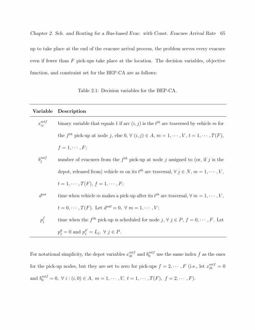
Chapter 2. Sch. and Routing for a Bus-based Evac. with Const. Evacuee Arrival Rate 65
up to take place at the end of the evacuee arrival process, the problem serves every evacuee
even if fewer than F pick-ups take place at the location. The decision variables, objective
function, and constraint set for the BEP-CA are as follows:
Table 2.1: Decision variables for the BEP-CA.
Variable Description
xmtfij binary variable that equals 1 if arc (i, j) is the tth arc traversed by vehicle m for
the f th pick-up at node j, else 0, ∀ (i, j) ∈ A, m = 1, · · · , V , t = 1, · · · , T (F ),
f = 1, · · · , F ;
bmtfj number of evacuees from the f th pick-up at node j assigned to (or, if j is the
depot, released from) vehicle m on its tth arc traversal, ∀ j ∈ N , m = 1, · · · , V ,
t = 1, · · · , T (F ), f = 1, · · · , F ;
dmt time when vehicle m makes a pick-up after its tth arc traversal, ∀m = 1, · · · , V ,
t = 0, · · · , T (F ). Let dm0 = 0, ∀ m = 1, · · · , V ;
pfj time when the f th pick-up is scheduled for node j, ∀ j ∈ P , f = 0, · · · , F . Let
p0j = 0 and pFj = Lj, ∀ j ∈ P .
For notational simplicity, the depot variables xmtfi0 and bmtf0 use the same index f as the ones
for the pick-up nodes, but they are set to zero for pick-ups f = 2, · · · , F (i.e., let xmtfi0 = 0
and bmtf0 = 0, ∀ i : (i, 0) ∈ A, m = 1, · · · , V, t = 1, · · · , T (F ), f = 2, · · · , F ).
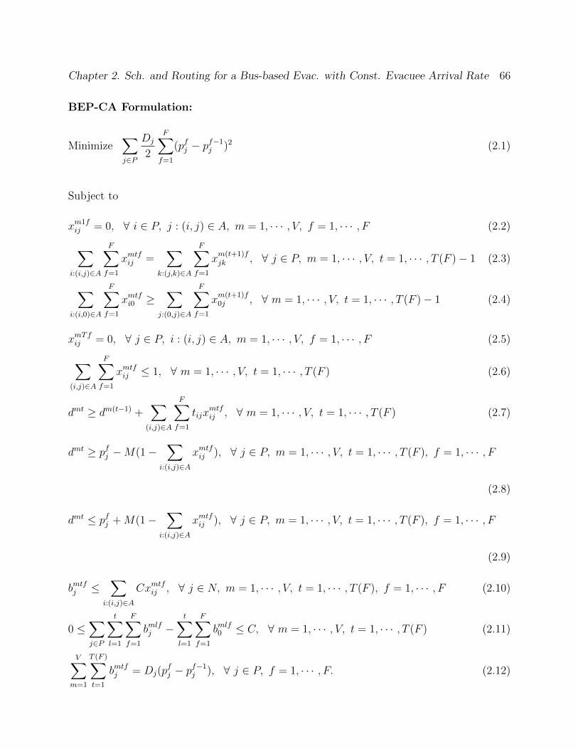
Chapter 2. Sch. and Routing for a Bus-based Evac. with Const. Evacuee Arrival Rate 66
BEP-CA Formulation:
Minimize∑
j∈P
Dj
2
F∑
f=1
(pfj − pf−1j )2 (2.1)
Subject to
xm1fij = 0, ∀ i ∈ P, j : (i, j) ∈ A, m = 1, · · · , V, f = 1, · · · , F (2.2)
∑
i:(i,j)∈A
F∑
f=1
xmtfij =∑
k:(j,k)∈A
F∑
f=1
xm(t+1)fjk , ∀ j ∈ P, m = 1, · · · , V, t = 1, · · · , T (F )− 1 (2.3)
∑
i:(i,0)∈A
F∑
f=1
xmtfi0 ≥∑
j:(0,j)∈A
F∑
f=1
xm(t+1)f0j , ∀ m = 1, · · · , V, t = 1, · · · , T (F )− 1 (2.4)
xmTfij = 0, ∀ j ∈ P, i : (i, j) ∈ A, m = 1, · · · , V, f = 1, · · · , F (2.5)
∑
(i,j)∈A
F∑
f=1
xmtfij ≤ 1, ∀ m = 1, · · · , V, t = 1, · · · , T (F ) (2.6)
dmt ≥ dm(t−1) +∑
(i,j)∈A
F∑
f=1
tijxmtfij , ∀ m = 1, · · · , V, t = 1, · · · , T (F ) (2.7)
dmt ≥ pfj −M(1−∑
i:(i,j)∈A
xmtfij ), ∀ j ∈ P, m = 1, · · · , V, t = 1, · · · , T (F ), f = 1, · · · , F
(2.8)
dmt ≤ pfj +M(1−∑
i:(i,j)∈A
xmtfij ), ∀ j ∈ P, m = 1, · · · , V, t = 1, · · · , T (F ), f = 1, · · · , F
(2.9)
bmtfj ≤∑
i:(i,j)∈A
Cxmtfij , ∀ j ∈ N, m = 1, · · · , V, t = 1, · · · , T (F ), f = 1, · · · , F (2.10)
0 ≤∑
j∈P
t∑
l=1
F∑
f=1
bmlfj −t∑
l=1
F∑
f=1
bmlf0 ≤ C, ∀ m = 1, · · · , V, t = 1, · · · , T (F ) (2.11)
V∑
m=1
T (F )∑
t=1
bmtfj = Dj(pfj − pf−1
j ), ∀ j ∈ P, f = 1, · · · , F. (2.12)

Chapter 2. Sch. and Routing for a Bus-based Evac. with Const. Evacuee Arrival Rate 67
Objective Function (2.1) minimizes the total exposure, that is, the weighted sum of the
squared time intervals between successive pick-ups at each pick-up node. Since evacuees are
assumed to gather at these nodes at a constant rate, Dj, and since the constraint set for
the BEP-CA forces buses to pick-up all evacuees that have arrived since the last pick-up,
(2.1) minimizes the total evacuee waiting time (i.e., the time between the arrival of each
evacuee and the subsequent scheduled pick-up, in units of people × minute, for example).
Constraints (2.2)-(2.6) ensure the construction of valid routes, including the elimination of
subtours. Constraint (2.2) prevents a vehicle’s first arc traversal (t = 1) from starting at a
pick-up node. Constraint (2.3) forces a vehicle’s (t + 1)th arc traversal to start from node
j ∈ P , if the vehicle’s tth arc traversal ended at node j. Constraint (2.4) is similar to (2.3),
but it allows vehicles to end service at the depot. Constraint (2.5) forces a vehicle’s T (F )th
arc traversal, if used, to end at the depot, and, finally, (2.6) limits vehicles to one pick-up per
arc traversal. Constraints (2.7)-(2.9) generate the pick-up schedule. Constraint (2.7) ensures
that the travel time for a vehicle is appropriately incremented after each arc traversal, while
(2.8) and (2.9) coordinate the arrival time of vehicles assigned to the f th scheduled pick-up at
node j. Here, let M = maxj∈P{Lj}+ max(i,j)∈A{tij}. Constraint (2.10) prevents a bus from
picking-up (or dropping-off) evacuees from a node unless the bus is at the node, while (2.11)
enforces the bus capacity restriction, allowing for multiple drop-offs at the depot. Constraint
(2.12) ensures that every evacuee waiting at a pick-up node is picked-up at the next scheduled
pick-up, and prevents higher index scheduled pick-ups from happening before lower index
ones, that is, it forces pfj ≥ pf−1j , ∀ j ∈ P, f = 1 · · ·F . Observe that the sequential pick-up

Chapter 2. Sch. and Routing for a Bus-based Evac. with Const. Evacuee Arrival Rate 68
ordering restriction is only locally enforced, for instance, a vehicle can go from the second
pick-up at node i to the first pick-up at node j. In addition, (2.12), along with the variable
restriction pFj = Lj, ∀ j ∈ P , ensure that every evacuee at pick-up node j is picked-up by
time Lj. Finally, the binary restriction on the x-variables and the non-negativity restriction
on the b, d, and p-variables are included.
As examples of the BEP-CA network structure, consider Scenarios 1 and 2 depicted in Figures
2.1(a) and 2.1(b), respectively, where buses have capacity of C = 20 evacuees. Observe that
these networks are complete, and that all arc traversal times satisfy the triangle inequality.
7
4
5
2
3
0
4
6 4
4
5
2
1
0
3
6
1
3
(a) (b)
5 4
Figure 2.1: The networks for Scenarios 1 (a) and 2 (b).
This formulation has two important properties. First, Lemma 2.1 shows that (2.1) is strictly
convex. Unfortunately, since the x-variables are binary, the resulting feasible region is non-
convex. Therefore, despite the use of a strictly convex objective function, multiple optimal

Chapter 2. Sch. and Routing for a Bus-based Evac. with Const. Evacuee Arrival Rate 69
solutions may exist for this problem, an intuitive finding considering its inheriting (and com-
plex) symmetries. Nonetheless, since (2.1) is strictly convex, every local minimum solution
is also a global minimum, and since this objective function is also twice differentiable, several
standard algorithms can be used to identify the optimal solution for the problem. Second,
Lemma 2.2 presents a necessary condition the problem feasibility. Note, however, that this
condition is not sufficient, as it ignores (2.2)-(2.6), the route construction constraints; (2.10),
the pick-up/drop-off constraint; and (2.11), the vehicle capacity constraint.
Lemma 2.1 Objective Function (2.1) is strictly convex.
Proof. See Appendix.
Lemma 2.2 The pick-up schedule 0 = p0j < t0j ≤ p1
j ≤ · · · ≤ pFj = Lj, ∀ j ∈ P is a
necessary condition for the BEP-CA feasibility.
Proof. See Appendix.
Next, Section 2.3 identifies and examines several properties of the BEP-CA.
2.3 Model Analysis
This section explores the effect of the maximum service level, F , and fleet size, V , over the
problem feasibility and the total exposure objective function value. Specifically, it is shown
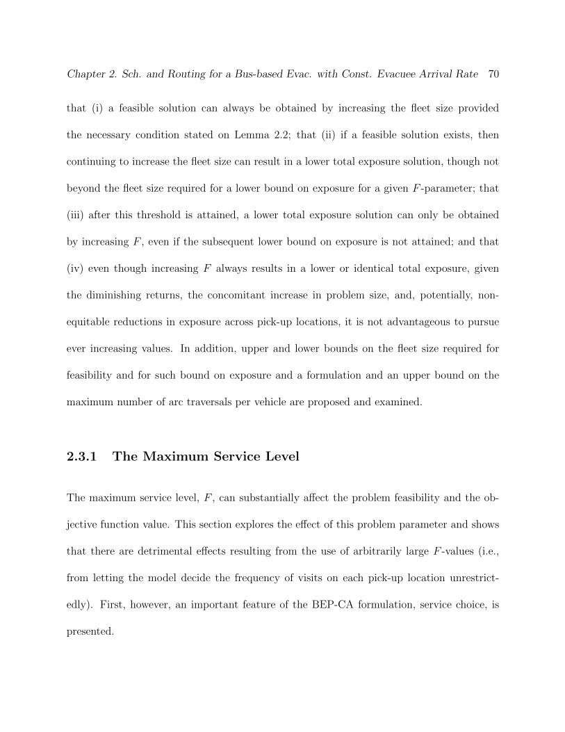
Chapter 2. Sch. and Routing for a Bus-based Evac. with Const. Evacuee Arrival Rate 70
that (i) a feasible solution can always be obtained by increasing the fleet size provided
the necessary condition stated on Lemma 2.2; that (ii) if a feasible solution exists, then
continuing to increase the fleet size can result in a lower total exposure solution, though not
beyond the fleet size required for a lower bound on exposure for a given F -parameter; that
(iii) after this threshold is attained, a lower total exposure solution can only be obtained
by increasing F , even if the subsequent lower bound on exposure is not attained; and that
(iv) even though increasing F always results in a lower or identical total exposure, given
the diminishing returns, the concomitant increase in problem size, and, potentially, non-
equitable reductions in exposure across pick-up locations, it is not advantageous to pursue
ever increasing values. In addition, upper and lower bounds on the fleet size required for
feasibility and for such bound on exposure and a formulation and an upper bound on the
maximum number of arc traversals per vehicle are proposed and examined.
2.3.1 The Maximum Service Level
The maximum service level, F , can substantially affect the problem feasibility and the ob-
jective function value. This section explores the effect of this problem parameter and shows
that there are detrimental effects resulting from the use of arbitrarily large F -values (i.e.,
from letting the model decide the frequency of visits on each pick-up location unrestrict-
edly). First, however, an important feature of the BEP-CA formulation, service choice, is
presented.
Chapter 2. Sch. and Routing for a Bus-based Evac. with Const. Evacuee Arrival Rate 71
2.3.1.1 Service Choice.
The BEP-CA exploits efficiencies deriving from service choice, that is, from letting F be an
upper bound on the number of pick-ups at each pick-up node. Since service choice increases
the size of the feasible region, it allows certain instances of the problem to become feasible
or to yield lower total exposure solutions. Example 2.1 presents one such instance.
Example 2.1 Consider the network displayed in Figure 2.2(a), with parameters F = 3
pick-ups, V = 3 buses, and C = 20 evacuees/bus. Depictions of the corresponding optimal
pick-up schedules without service choice (at time p11 = 1, p2
1 = 1.5, p31 = L1 = 2 and
p12 = 5, p2
2 = 5.5, p32 = L2 = 6) and with service choice (at time p1
1 = 1, p21 = L1 = 2 and
p12 = 4, p2
2 = 5, p32 = L2 = 6) are presented in Figures 2.2(b) and 2.2(c), respectively. In
these figures, solid lines indicate periods when buses are idle, whereas dashed lines indicate
periods when buses are moving. The number of evacuees on the bus, if any, is presented on
top of the dashed lines. Although it would appear that the lowest total exposure solution is
obtained when all F pick-ups take place, as these figures exemplify, enforcing all F pick-ups
may result in a higher exposure solution than the one obtained from allowing service choice
(27 versus 20). Moreover, note that if F is increased (i.e., if F ≥ 4), if service choice is
not allowed, and if the fleet size remains unchanged (i.e., if V = 3 buses), then the problem
becomes infeasible.
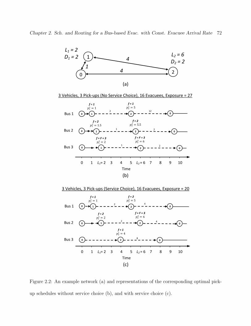
Chapter 2. Sch. and Routing for a Bus-based Evac. with Const. Evacuee Arrival Rate 72
3 Vehicles, 3 Pick-ups (Service Choice), 16 Evacuees, Exposure = 20
3 Vehicles, 3 Pick-ups (No Service Choice), 16 Evacuees, Exposure = 27
f = 1
f = 1
Bus 1
Bus 2
0 2 0
0
1
0
2 evac
1
Bus 3 0
1
1
f = 2
f = F = 3
2
0 2 1
f = 2
f = F = 3
12 evac
2
2
f = 1
f = 2
Bus 1
Bus 2
0 2 0
0
1
0
2 evac
2
Bus 3 0
1
f = 2
2
0 2
f = 1
4 evac
4
8
2
1 L2 = 6 D2 = 2
(a)
0
1 4
L1 = 2 D1 = 2
4
f = F = 3
(b)
Time
10 1 L2 = 6 0 5 L1= 2 9 3 4 7 8
(c)
Time
10 1 L2 = 6 0 5 L1= 2 9 3 4 7 8
Figure 2.2: An example network (a) and representations of the corresponding optimal pick-
up schedules without service choice (b), and with service choice (c).
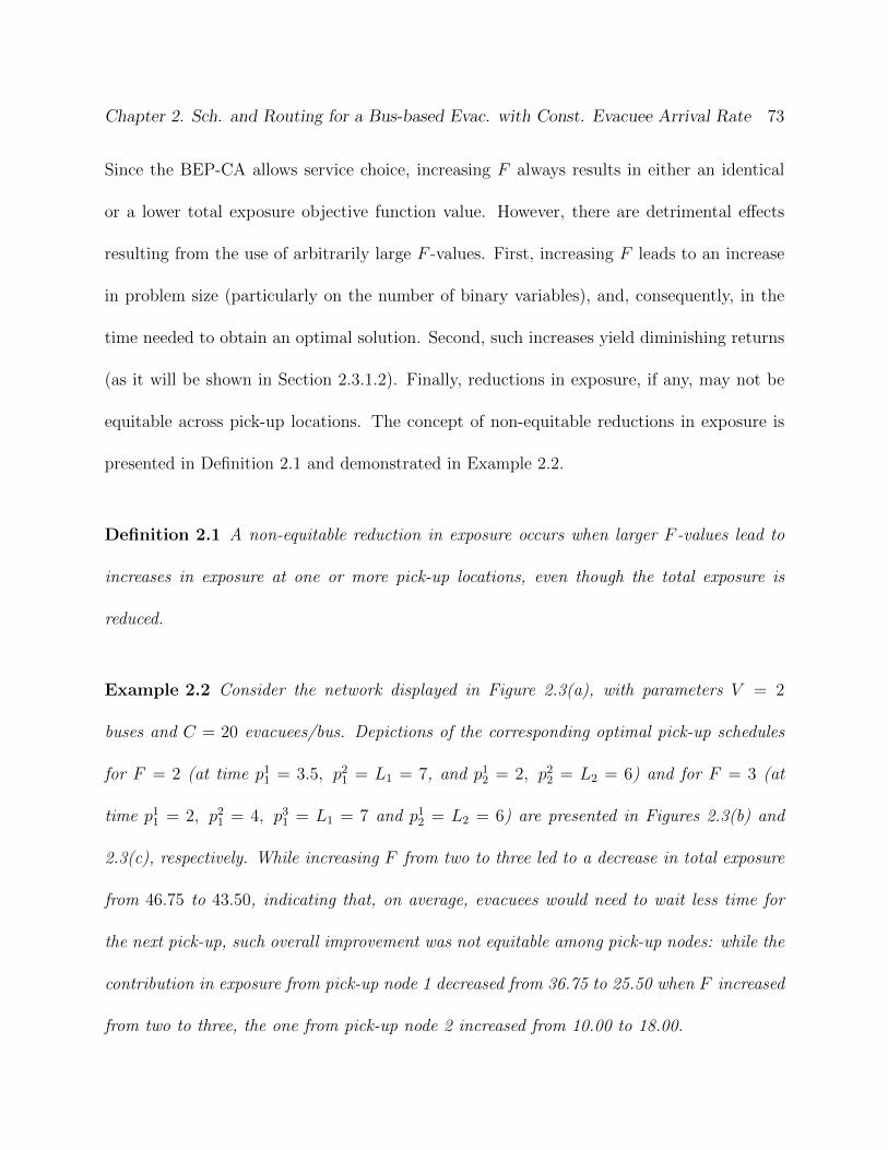
Chapter 2. Sch. and Routing for a Bus-based Evac. with Const. Evacuee Arrival Rate 73
Since the BEP-CA allows service choice, increasing F always results in either an identical
or a lower total exposure objective function value. However, there are detrimental effects
resulting from the use of arbitrarily large F -values. First, increasing F leads to an increase
in problem size (particularly on the number of binary variables), and, consequently, in the
time needed to obtain an optimal solution. Second, such increases yield diminishing returns
(as it will be shown in Section 2.3.1.2). Finally, reductions in exposure, if any, may not be
equitable across pick-up locations. The concept of non-equitable reductions in exposure is
presented in Definition 2.1 and demonstrated in Example 2.2.
Definition 2.1 A non-equitable reduction in exposure occurs when larger F -values lead to
increases in exposure at one or more pick-up locations, even though the total exposure is
reduced.
Example 2.2 Consider the network displayed in Figure 2.3(a), with parameters V = 2
buses and C = 20 evacuees/bus. Depictions of the corresponding optimal pick-up schedules
for F = 2 (at time p11 = 3.5, p2
1 = L1 = 7, and p12 = 2, p2
2 = L2 = 6) and for F = 3 (at
time p11 = 2, p2
1 = 4, p31 = L1 = 7 and p1
2 = L2 = 6) are presented in Figures 2.3(b) and
2.3(c), respectively. While increasing F from two to three led to a decrease in total exposure
from 46.75 to 43.50, indicating that, on average, evacuees would need to wait less time for
the next pick-up, such overall improvement was not equitable among pick-up nodes: while the
contribution in exposure from pick-up node 1 decreased from 36.75 to 25.50 when F increased
from two to three, the one from pick-up node 2 increased from 10.00 to 18.00.
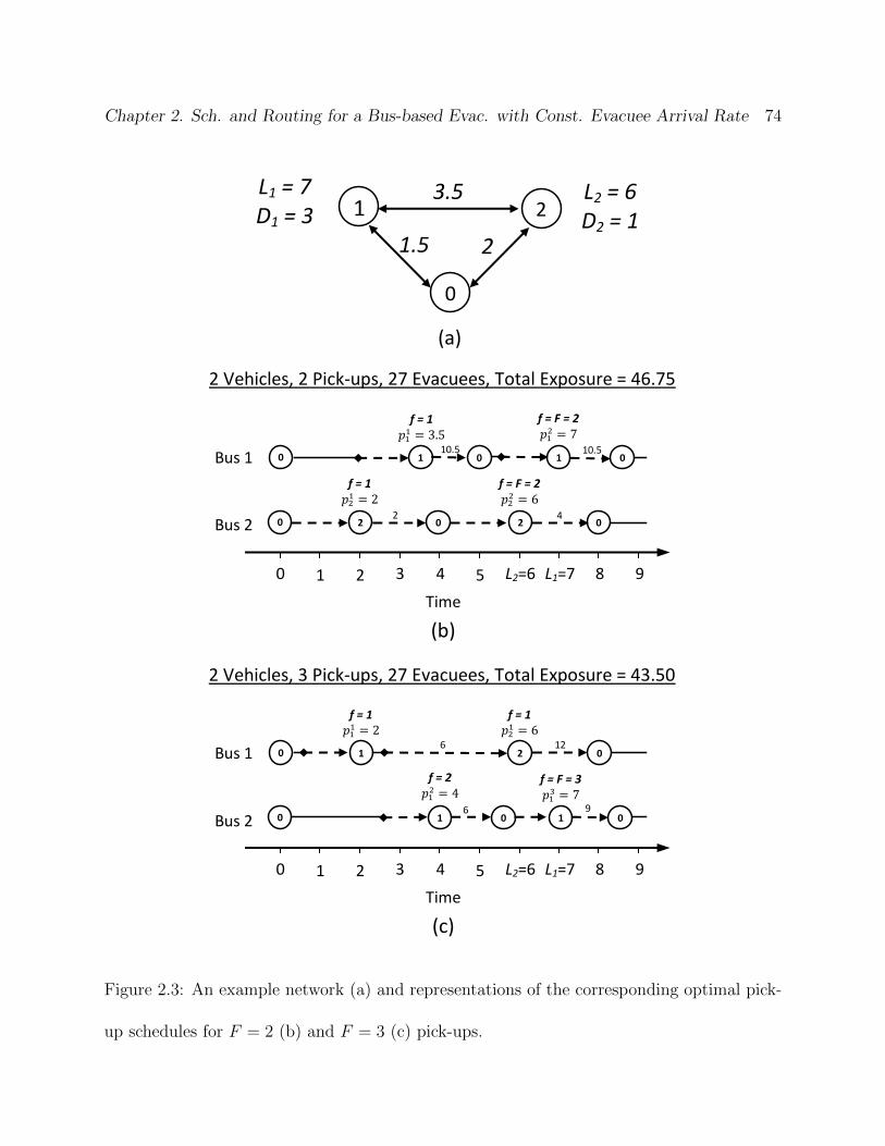
Chapter 2. Sch. and Routing for a Bus-based Evac. with Const. Evacuee Arrival Rate 74
2 1 3.5 L2 = 6
D2 = 1
(a)
0
2 1.5
L1 = 7 D1 = 3
2 Vehicles, 2 Pick-ups, 27 Evacuees, Total Exposure = 46.75
f = F = 2
f = F = 2
Bus 1 0
2
0 1
2 2
Time
(b)
1
0
10.5
4
10.5
f = 1
f = 1
2 Vehicles, 3 Pick-ups, 27 Evacuees, Total Exposure = 43.50
L1=7 1 3 4 0 8 L2=6 2 5 9
Bus 2 0 0
0
f = 1
f = F = 3
Bus 1 0
0
0
1
Time
(c)
1
1
12
6
6
f = 1
f = 2
9 5 2 L2=6 8 0 4 3 1 L1=7
Bus 2 0 0
2
9
Figure 2.3: An example network (a) and representations of the corresponding optimal pick-
up schedules for F = 2 (b) and F = 3 (c) pick-ups.
Chapter 2. Sch. and Routing for a Bus-based Evac. with Const. Evacuee Arrival Rate 75
In addition, since the BEP-CA assumes that evacuees arrive linearly at the various pick-up
locations, some individuals may need to wait longer under larger F -values, even in pick-up
nodes having reduced exposure, higher frequency of visits, or, even, a reduction in the largest
interval between bus arrivals. For instance, an individual that arrived on pick-up node 1 at
time 3 would need to wait 0.5 time units for the next pick-up under F = 2 and 1 time unit
under F = 3. These differences, however, are not related to the definition of equity used for
the purposes of this research.
As demonstrated in Example 2.2, service choice, albeit often desirable, can also lead to
non-equitable reductions in exposure across pick-up locations. While it is easy to enforce
F pick-ups on each location, such a constraint, by itself, would not solve the issue due to
the difficult in differentiating between relatively close scheduled pick-up times. For instance,
suppose that F = 2, then the optimal pick-up schedule at a given location may consist of
a single visit by two vehicles, say at time Lj = 10. If service choice is prevented, then the
optimal pick-up schedule may consist of two visits by one vehicle each, say at times 9.9 and
10. Since both schedules are virtually identical, neither one addresses the issue. Generally,
such can only be prevented by fixing the p-variables to an equitable pick-up schedule before
the problem is optimized. However, by limiting the size of the feasible region, such approach
may lead to infeasibility or worsen the objective function value. The next section introduces
and examines the pick-up schedule resulting in the lowest exposure for a given F -value.
Among other properties, it is shown that such pick-up schedule, when feasible, guarantees
equitable reductions in exposure across pick-up locations.
Chapter 2. Sch. and Routing for a Bus-based Evac. with Const. Evacuee Arrival Rate 76
The next section introduces and examines the pick-up schedule resulting in the lowest ex-
posure for a given F -value. Among other properties, it is shown that such pick-up schedule,
when feasible, guarantees equitable reductions in exposure across pick-up locations.
2.3.1.2 The Minimum Exposure Schedule.
The Minimum Exposure Schedule for a given F -parameter, MES(F ), is defined as follows:
Definition 2.2 The MES(F ) is the pick-up schedule that minimizes (2.1) subject only to
the necessary condition for feasibility presented in Lemma 2.2.
The MES(F ) can be obtained by the following formulation:
Minimize∑
j∈P
F∑
f=1
1
2Djq
fj
2(2.13)
subject toF∑
f=1
qfj = Lj, ∀ j ∈ P (2.14)
q1j ≥ t0j, ∀ j ∈ P (2.15)
qfj ≥ 0, ∀ j ∈ P, f = 1, · · · , F, (2.16)
where qfj denotes the interval between scheduled pick-up times at pick-up node j (i.e., qfj =
pfj − pf−1j , ∀ j ∈ P, f = 1, · · · , F ). Objective Function (2.13) follows from (2.1), and
Constraints (2.14)-(2.16) enforce the necessary condition presented in Lemma 2.2. Since
this condition is not sufficient, the MES(F ) yields a lower bound on (2.1), and will only
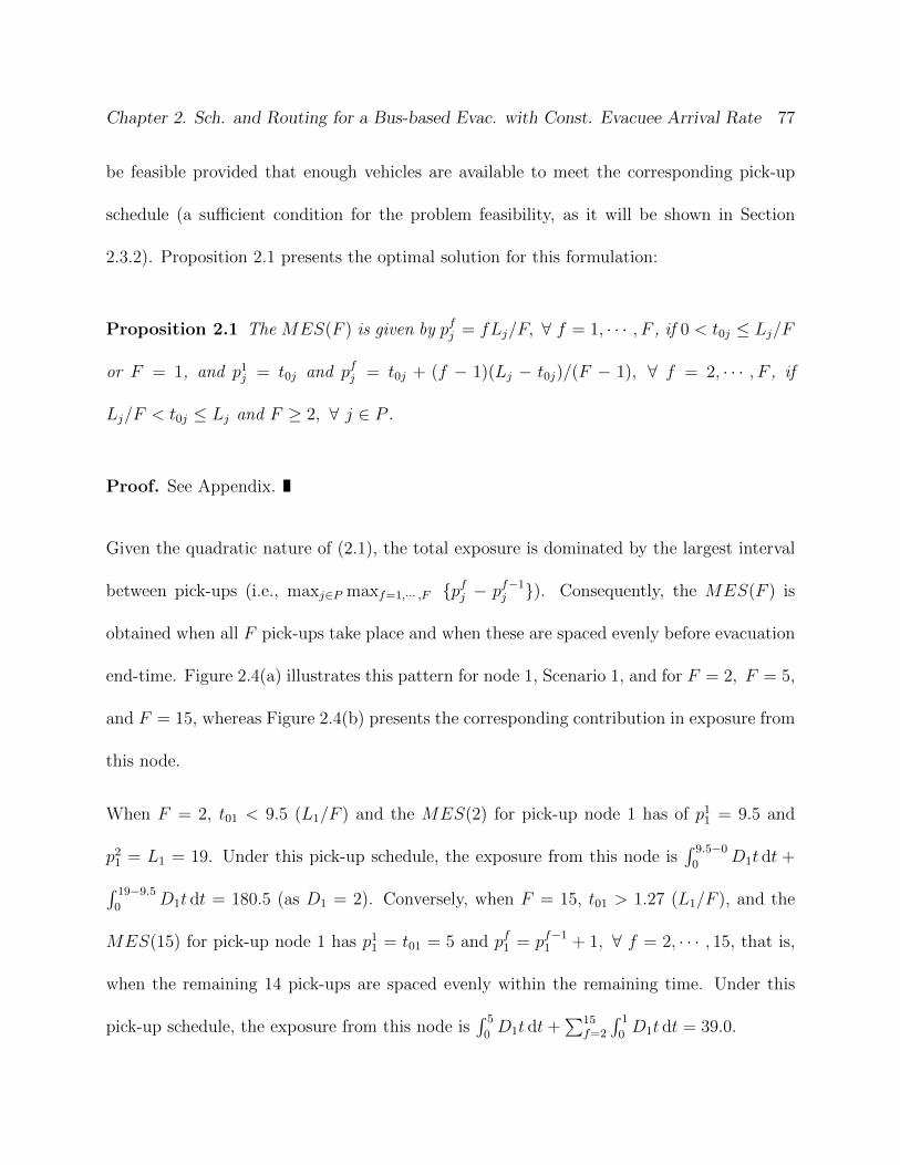
Chapter 2. Sch. and Routing for a Bus-based Evac. with Const. Evacuee Arrival Rate 77
be feasible provided that enough vehicles are available to meet the corresponding pick-up
schedule (a sufficient condition for the problem feasibility, as it will be shown in Section
2.3.2). Proposition 2.1 presents the optimal solution for this formulation:
Proposition 2.1 The MES(F ) is given by pfj = fLj/F, ∀ f = 1, · · · , F , if 0 < t0j ≤ Lj/F
or F = 1, and p1j = t0j and pfj = t0j + (f − 1)(Lj − t0j)/(F − 1), ∀ f = 2, · · · , F , if
Lj/F < t0j ≤ Lj and F ≥ 2, ∀ j ∈ P .
Proof. See Appendix.
Given the quadratic nature of (2.1), the total exposure is dominated by the largest interval
between pick-ups (i.e., maxj∈P maxf=1,··· ,F {pfj − pf−1j }). Consequently, the MES(F ) is
obtained when all F pick-ups take place and when these are spaced evenly before evacuation
end-time. Figure 2.4(a) illustrates this pattern for node 1, Scenario 1, and for F = 2, F = 5,
and F = 15, whereas Figure 2.4(b) presents the corresponding contribution in exposure from
this node.
When F = 2, t01 < 9.5 (L1/F ) and the MES(2) for pick-up node 1 has of p11 = 9.5 and
p21 = L1 = 19. Under this pick-up schedule, the exposure from this node is
∫ 9.5−0
0D1t dt +
∫ 19−9.5
0D1t dt = 180.5 (as D1 = 2). Conversely, when F = 15, t01 > 1.27 (L1/F ), and the
MES(15) for pick-up node 1 has p11 = t01 = 5 and pf1 = pf−1
1 + 1, ∀ f = 2, · · · , 15, that is,
when the remaining 14 pick-ups are spaced evenly within the remaining time. Under this
pick-up schedule, the exposure from this node is∫ 5
0D1t dt+
∑15f=2
∫ 1
0D1t dt = 39.0.
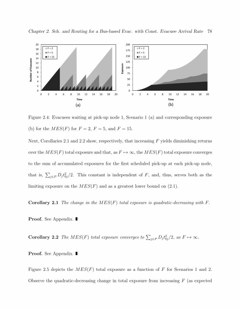
Chapter 2. Sch. and Routing for a Bus-based Evac. with Const. Evacuee Arrival Rate 78
0
2
4
6
8
10
12
14
16
18
20
0 2 4 6 8 10 12 14 16 18 20
Nu
mb
er o
f Ev
acu
ees
Time
F = 2
F = 5
F = 15
0
25
50
75
100
125
150
175
200
0 2 4 6 8 10 12 14 16 18 20
Exp
osu
re
Time
F = 2
F = 5
F = 15
(a) (b)
Figure 2.4: Evacuees waiting at pick-up node 1, Scenario 1 (a) and corresponding exposure
(b) for the MES(F ) for F = 2, F = 5, and F = 15.
Next, Corollaries 2.1 and 2.2 show, respectively, that increasing F yields diminishing returns
over theMES(F ) total exposure and that, as F 7→ ∞, theMES(F ) total exposure converges
to the sum of accumulated exposures for the first scheduled pick-up at each pick-up node,
that is,∑
j∈P Djt20j/2. This constant is independent of F , and, thus, serves both as the
limiting exposure on the MES(F ) and as a greatest lower bound on (2.1).
Corollary 2.1 The change in the MES(F ) total exposure is quadratic-decreasing with F .
Proof. See Appendix.
Corollary 2.2 The MES(F ) total exposure converges to∑
j∈P Djt20j/2, as F 7→ ∞.
Proof. See Appendix.
Figure 2.5 depicts the MES(F ) total exposure as a function of F for Scenarios 1 and 2.
Observe the quadratic-decreasing change in total exposure from increasing F (as expected
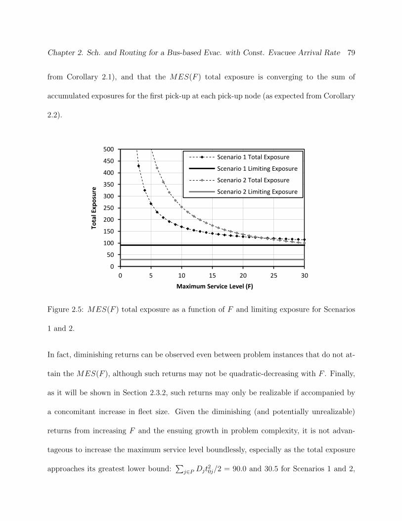
Chapter 2. Sch. and Routing for a Bus-based Evac. with Const. Evacuee Arrival Rate 79
from Corollary 2.1), and that the MES(F ) total exposure is converging to the sum of
accumulated exposures for the first pick-up at each pick-up node (as expected from Corollary
2.2).
0
50
100
150
200
250
300
350
400
450
500
0 5 10 15 20 25 30
Tota
l Exp
osu
re
Maximum Service Level (F)
Scenario 1 Total Exposure
Scenario 1 Limiting Exposure
Scenario 2 Total Exposure
Scenario 2 Limiting Exposure
Figure 2.5: MES(F ) total exposure as a function of F and limiting exposure for Scenarios
1 and 2.
In fact, diminishing returns can be observed even between problem instances that do not at-
tain the MES(F ), although such returns may not be quadratic-decreasing with F . Finally,
as it will be shown in Section 2.3.2, such returns may only be realizable if accompanied by
a concomitant increase in fleet size. Given the diminishing (and potentially unrealizable)
returns from increasing F and the ensuing growth in problem complexity, it is not advan-
tageous to increase the maximum service level boundlessly, especially as the total exposure
approaches its greatest lower bound:∑
j∈P Djt20j/2 = 90.0 and 30.5 for Scenarios 1 and 2,
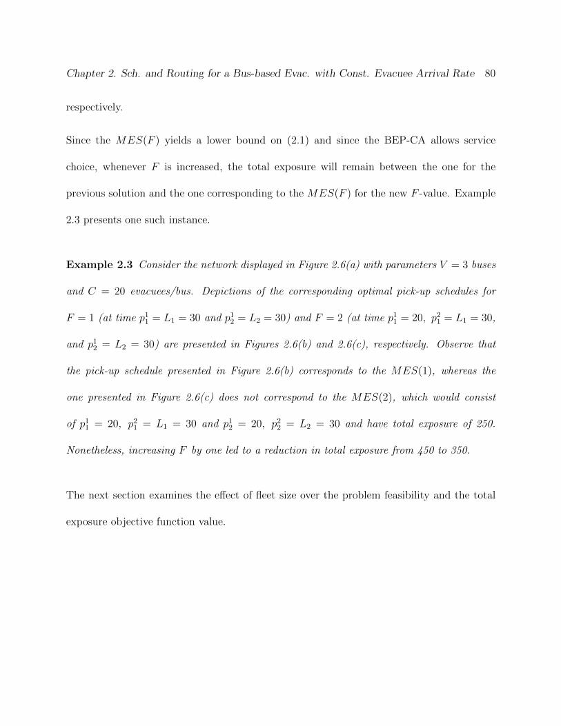
Chapter 2. Sch. and Routing for a Bus-based Evac. with Const. Evacuee Arrival Rate 80
respectively.
Since the MES(F ) yields a lower bound on (2.1) and since the BEP-CA allows service
choice, whenever F is increased, the total exposure will remain between the one for the
previous solution and the one corresponding to the MES(F ) for the new F -value. Example
2.3 presents one such instance.
Example 2.3 Consider the network displayed in Figure 2.6(a) with parameters V = 3 buses
and C = 20 evacuees/bus. Depictions of the corresponding optimal pick-up schedules for
F = 1 (at time p11 = L1 = 30 and p1
2 = L2 = 30) and F = 2 (at time p11 = 20, p2
1 = L1 = 30,
and p12 = L2 = 30) are presented in Figures 2.6(b) and 2.6(c), respectively. Observe that
the pick-up schedule presented in Figure 2.6(b) corresponds to the MES(1), whereas the
one presented in Figure 2.6(c) does not correspond to the MES(2), which would consist
of p11 = 20, p2
1 = L1 = 30 and p12 = 20, p2
2 = L2 = 30 and have total exposure of 250.
Nonetheless, increasing F by one led to a reduction in total exposure from 450 to 350.
The next section examines the effect of fleet size over the problem feasibility and the total
exposure objective function value.

Chapter 2. Sch. and Routing for a Bus-based Evac. with Const. Evacuee Arrival Rate 81
2 1 20 L2 = 30
D2 = 0.5
(a)
(c)
0
20 20
L1 = 30 D1 = 0.5
Time
60 10 20 L1=L2=30 0 40 50
3 Vehicles, 2 Pick-ups, 30 Evacuees, Total Exposure = 350
f = 1
f = 1
Bus 1
Bus 2
0 2 0
0 1 0
15 evac
10
f = F = 2
Bus 3 0 1 0 5
3 Vehicles, 1 Pick-up, 30 Evacuees, Total Exposure = 450
f = F = 1
f = F = 1
Bus 1
Bus 2
0 2 0
0 1 0
15 evac
15
Bus 3 0
Time
60 10 20 L1=L2=30 0 40 50
(b)
Figure 2.6: An example network (a) and representations of the corresponding optimal pick-
up schedules for F = 1 (b) and F = 2 (c) pick-ups.
Chapter 2. Sch. and Routing for a Bus-based Evac. with Const. Evacuee Arrival Rate 82
2.3.2 Fleet Size
In this section, an alternative objective function to minimize fleet size, as well as upper and
lower bounds on the fleet size needed for a feasible implementation of the MES(F ) and for
a feasible solution to the BEP-CA are presented and examined.
Similar to the maximum service level, F , the fleet size parameter, V , can also influence
feasibility and the total exposure objective function value. First, since the BEP-CA allows
service choice, if enough vehicles are available, then it is feasible to pick-up all∑
j∈P DjLj
evacuees in one pick-up. Consequently, a feasible solution can always be obtained by in-
creasing the fleet size provided the necessary condition stated on Lemma 2.2. Moreover, if
multiple pick-ups are feasible (i.e., if F ≥ 2 and if enough vehicles are available to meet the
extra pick-ups), then a lower exposure pick-up schedule may also be feasible. For instance,
in the network for Scenario 1, 38 evacuees must be picked-up in node 1, 44 in node 2, and 42
in node 3 (for a total of 124 evacuees). Hence a feasible solution would be to send 2 buses to
node 1 (arriving at time p11 = L1 = 19), 3 buses to node 2 (arriving at time p1
2 = L2 = 22),
and 3 buses to node 3 (arriving at time p13 = L3 = 21) for a total exposure of 1286. However,
as it will be shown later, the MES(8) is feasible for the same number of vehicles, resulting
in a total exposure of 191.4. Next, an alternative objective function to minimize the fleet
size parameter, V , is introduced.
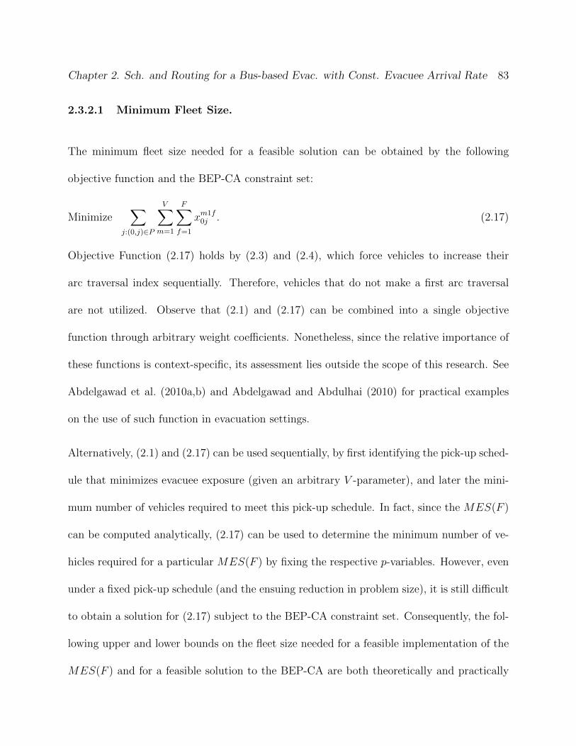
Chapter 2. Sch. and Routing for a Bus-based Evac. with Const. Evacuee Arrival Rate 83
2.3.2.1 Minimum Fleet Size.
The minimum fleet size needed for a feasible solution can be obtained by the following
objective function and the BEP-CA constraint set:
Minimize∑
j:(0,j)∈P
V∑
m=1
F∑
f=1
xm1f0j . (2.17)
Objective Function (2.17) holds by (2.3) and (2.4), which force vehicles to increase their
arc traversal index sequentially. Therefore, vehicles that do not make a first arc traversal
are not utilized. Observe that (2.1) and (2.17) can be combined into a single objective
function through arbitrary weight coefficients. Nonetheless, since the relative importance of
these functions is context-specific, its assessment lies outside the scope of this research. See
Abdelgawad et al. (2010a,b) and Abdelgawad and Abdulhai (2010) for practical examples
on the use of such function in evacuation settings.
Alternatively, (2.1) and (2.17) can be used sequentially, by first identifying the pick-up sched-
ule that minimizes evacuee exposure (given an arbitrary V -parameter), and later the mini-
mum number of vehicles required to meet this pick-up schedule. In fact, since the MES(F )
can be computed analytically, (2.17) can be used to determine the minimum number of ve-
hicles required for a particular MES(F ) by fixing the respective p-variables. However, even
under a fixed pick-up schedule (and the ensuing reduction in problem size), it is still difficult
to obtain a solution for (2.17) subject to the BEP-CA constraint set. Consequently, the fol-
lowing upper and lower bounds on the fleet size needed for a feasible implementation of the
MES(F ) and for a feasible solution to the BEP-CA are both theoretically and practically

Chapter 2. Sch. and Routing for a Bus-based Evac. with Const. Evacuee Arrival Rate 84
relevant.
2.3.2.2 Upper Bound on the MES(F ) Fleet Size.
Proposition 2.2 presents an analytical upper bound on the fleet size needed for a feasible
implementation of the MES(F ).
Proposition 2.2 The upper bound on the fleet size needed for a feasible implementation of
the MES(F ), VUB(F ), is calculated as follows:
VUB(F ) =∑
j∈P
(⌈Djλj(F )
C
⌉+
(min
{⌈2t0jτj(F )
⌉, F
}− 1
)⌈Djτj(F )
C
⌉), (2.18)
where τj(F ) and λj(F ) are, respectively, the smallest and largest intervals between scheduled
pick-up times at pick-up node j under the MES(F ), that is, τj(F ) = minf=1,··· ,F{pfj−pf−1j } =
min{Lj/F, (Lj − t0j)/(F − 1)} and λj(F ) = maxf=1,··· ,F{pfj − pf−1j } = max{Lj/F, t0j}.
Proof. See Appendix.
Since the MES(F ) yields a lower bound on (2.1), increasing the fleet size beyond what is
required for its feasibility will never result in a lower exposure solution. Consequently, the
fleet size obtained from Proposition 2.2 yields the lowest exposure for a given F -parameter. In
addition, observe that VUB(F ) is tight whenever the MES(F ) is achieved and such solution
is attained by having vehicles dedicated to a single pick-up node. These properties are shown
in Example 2.4.
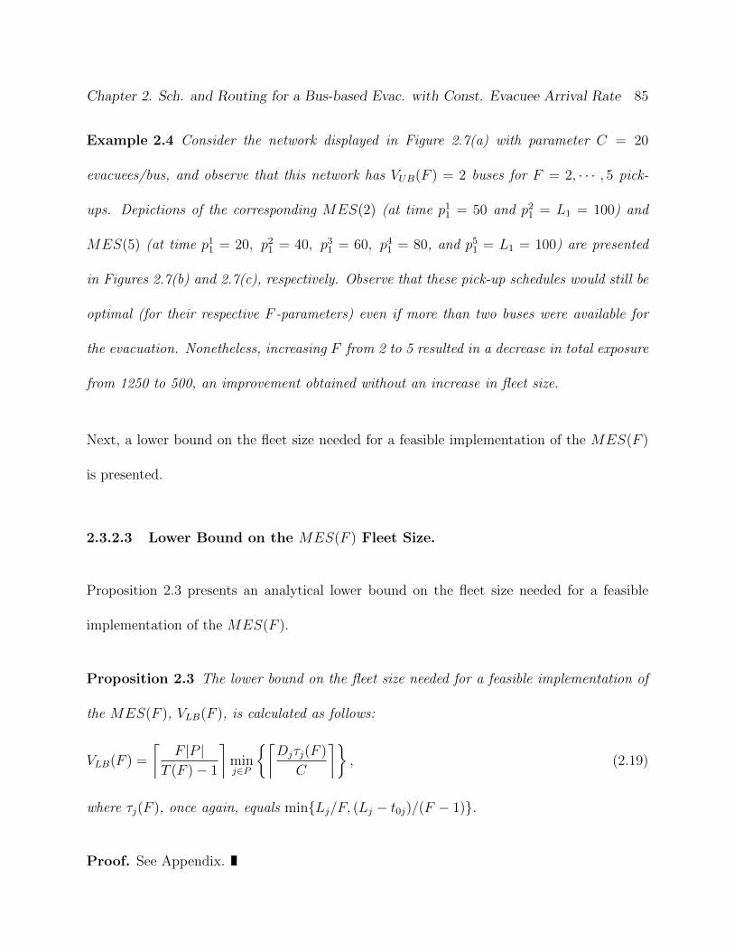
Chapter 2. Sch. and Routing for a Bus-based Evac. with Const. Evacuee Arrival Rate 85
Example 2.4 Consider the network displayed in Figure 2.7(a) with parameter C = 20
evacuees/bus, and observe that this network has VUB(F ) = 2 buses for F = 2, · · · , 5 pick-
ups. Depictions of the corresponding MES(2) (at time p11 = 50 and p2
1 = L1 = 100) and
MES(5) (at time p11 = 20, p2
1 = 40, p31 = 60, p4
1 = 80, and p51 = L1 = 100) are presented
in Figures 2.7(b) and 2.7(c), respectively. Observe that these pick-up schedules would still be
optimal (for their respective F -parameters) even if more than two buses were available for
the evacuation. Nonetheless, increasing F from 2 to 5 resulted in a decrease in total exposure
from 1250 to 500, an improvement obtained without an increase in fleet size.
Next, a lower bound on the fleet size needed for a feasible implementation of the MES(F )
is presented.
2.3.2.3 Lower Bound on the MES(F ) Fleet Size.
Proposition 2.3 presents an analytical lower bound on the fleet size needed for a feasible
implementation of the MES(F ).
Proposition 2.3 The lower bound on the fleet size needed for a feasible implementation of
the MES(F ), VLB(F ), is calculated as follows:
VLB(F ) =
⌈F |P |
T (F )− 1
⌉minj∈P
{⌈Djτj(F )
C
⌉}, (2.19)
where τj(F ), once again, equals min{Lj/F, (Lj − t0j)/(F − 1)}.
Proof. See Appendix.

Chapter 2. Sch. and Routing for a Bus-based Evac. with Const. Evacuee Arrival Rate 86
Time
120 20 40 60 0 80 L1 = 100
(c)
2 Vehicles, 5 Pick-ups, 50 Evacuees, Total Exposure = 500
f = 1
f = 3
f = F = 5
Bus 1 0 1 0 1 0 0 1 10 10 10
f = 2
f = 4
Bus 2 0 1 0 1 0 10 10
1 0 20 L1 = 100
D1 = 0.5
(a)
2 Vehicles, 2 Pick-ups, 50 Evacuees, Total Exposure = 1250
f = 1
f = F = 2
Bus 1
Bus 2
0 1 0 1 0
0 1 0
12.5 evac
12.5
12.5
Time
120 20 40 60 0 80 L1 = 100
(b)
1 0 12.5 evac
Figure 2.7: An example network (a) and representations of the corresponding MES(F ) for
F = 2 (b) and F = 5 (c).
This bound corresponds to the product of two factors: a lower bound on the number of
groups of buses simultaneously performing pick-ups under the MES(F ) and a lower bound
on the number of buses needed in each group in order to pick-up all evacuees that arrived
between scheduled pick-up times. Example 2.5 shows that, contrary to VUB(F ), the lower

Chapter 2. Sch. and Routing for a Bus-based Evac. with Const. Evacuee Arrival Rate 87
bound on the fleet size needed for a feasible implementation of the MES(F ) is not tight
in general, even in instances that achieve the MES(F ) with vehicles dedicated to a single
pick-up location.
Example 2.5 Recall the network presented in Example 2.4, Figure 2.7(a) with parameter
C = 20 evacuees/bus. Depictions of the corresponding MES(1) (at time p11 = L1 = 100)
and MES(3) (at time p11 = 33.3, p2
1 = 66.7, and p31 = L1 = 100) are presented in Figures
2.8(a) and 2.8(b), respectively. When F = 1, T (1) = 2 and τ1(1) = 100 ⇒ VLB(1) = 3, the
exact fleet size needed for a feasible implementation of the MES(1). However, when F = 3,
T (3) = 6 and τ1(3) = 33.3 ⇒ VLB(3) = 1, and, as depicted in Figure 2.8(b), at least two
vehicles are needed for a feasible implementation of the MES(3) when C = 20 evacuees/bus.
Next, the proposed upper and lower bounds on the fleet size needed for a feasible implemen-
tation of the MES(F ) are used to derive important relationships between the number of
available buses, the maximum service level, and the total exposure objective function value.
2.3.2.4 The MES(F ) Fleet Size.
This section explores the behavior of the exact fleet size needed for a feasible implemen-
tation of the MES(F ) based on its relationship with VUB(F ) and VLB(F ). Specifically, it
is shown that there exists an interval of F -values such that smaller F -values result in the
sub-utilization of the fleet available whereas larger F -values may result in non-equitable
reductions in exposure across pick-up locations.
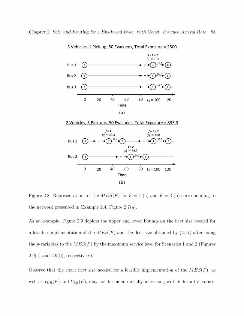
Chapter 2. Sch. and Routing for a Bus-based Evac. with Const. Evacuee Arrival Rate 88
3 Vehicles, 1 Pick-up, 50 Evacuees, Total Exposure = 2500
f = F = 1
Bus 1 0 1 0
16.7
Time
120 20 40 60 0 80 L1 = 100
(a)
Bus 2 0 1 0 16.7
Bus 3 0 1 0 16.7
2 Vehicles, 3 Pick-ups, 50 Evacuees, Total Exposure = 833.3
f = 1
f = 2
f = F = 3
Bus 1
Bus 2
0 1 0 1 0
0 1 0
16.7 evac
16.7
16.7
Time
120 20 40 60 0 80 L1 = 100
(b)
Figure 2.8: Representations of the MES(F ) for F = 1 (a) and F = 3 (b) corresponding to
the network presented in Example 2.4, Figure 2.7(a).
As an example, Figure 2.9 depicts the upper and lower bounds on the fleet size needed for
a feasible implementation of the MES(F ) and the fleet size obtained by (2.17) after fixing
the p-variables to the MES(F ) by the maximum service level for Scenarios 1 and 2 (Figures
2.9(a) and 2.9(b), respectively).
Observe that the exact fleet size needed for a feasible implementation of the MES(F ), as
well as VUB(F ) and VLB(F ), may not be monotonically increasing with F for all F -values.
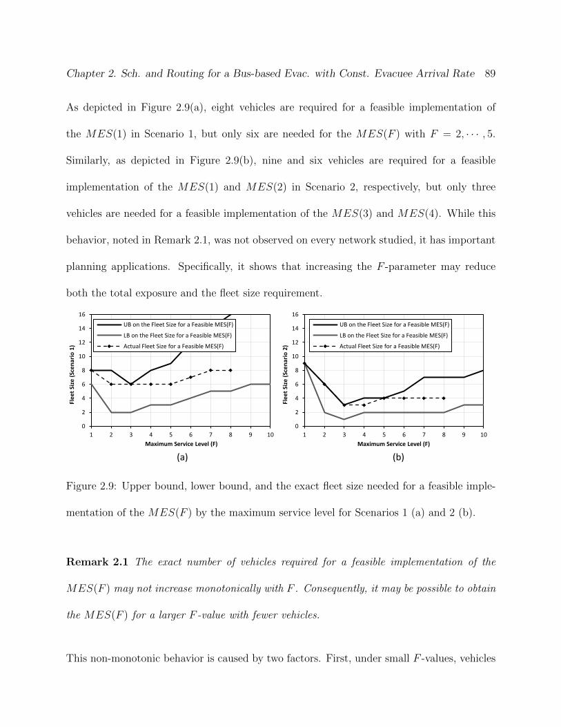
Chapter 2. Sch. and Routing for a Bus-based Evac. with Const. Evacuee Arrival Rate 89
As depicted in Figure 2.9(a), eight vehicles are required for a feasible implementation of
the MES(1) in Scenario 1, but only six are needed for the MES(F ) with F = 2, · · · , 5.
Similarly, as depicted in Figure 2.9(b), nine and six vehicles are required for a feasible
implementation of the MES(1) and MES(2) in Scenario 2, respectively, but only three
vehicles are needed for a feasible implementation of the MES(3) and MES(4). While this
behavior, noted in Remark 2.1, was not observed on every network studied, it has important
planning applications. Specifically, it shows that increasing the F -parameter may reduce
both the total exposure and the fleet size requirement.
0
2
4
6
8
10
12
14
16
1 2 3 4 5 6 7 8 9 10
Fle
et
Size
(Sc
en
ari
o 1
)
Maximum Service Level (F)
UB on the Fleet Size for a Feasible MES(F)
LB on the Fleet Size for a Feasible MES(F)
Actual Fleet Size for a Feasible MES(F)
0
2
4
6
8
10
12
14
16
1 2 3 4 5 6 7 8 9 10
Fle
et
Size
(Sc
en
ari
o 2
)
Maximum Service Level (F)
UB on the Fleet Size for a Feasible MES(F)
LB on the Fleet Size for a Feasible MES(F)
Actual Fleet Size for a Feasible MES(F)
(a) (b)
Figure 2.9: Upper bound, lower bound, and the exact fleet size needed for a feasible imple-
mentation of the MES(F ) by the maximum service level for Scenarios 1 (a) and 2 (b).
Remark 2.1 The exact number of vehicles required for a feasible implementation of the
MES(F ) may not increase monotonically with F . Consequently, it may be possible to obtain
the MES(F ) for a larger F -value with fewer vehicles.
This non-monotonic behavior is caused by two factors. First, under small F -values, vehicles

Chapter 2. Sch. and Routing for a Bus-based Evac. with Const. Evacuee Arrival Rate 90
may spend a considerable amount of time idle (i.e., stationed at the depot or at some pick-up
node). As F increases, the existing fleet is reused to meet the extra pick-ups and the excess
idle time diminishes. Second, the increased F -parameter (and consequent reduced interval
between scheduled pick-up times) results in a reduced number of evacuees waiting for each
bus arrival, and, thus, in an smaller number of buses that need to arrive simultaneously
in order to pick-up these evacuees. As F continues to increase, the excess idle time is
depleted, vehicles starts to run well under capacity, and the fleet size needed for a feasible
implementation of the MES(F ) once again starts to increase.
Clearly, the F -value (if one exists) where the fleet size needed for a feasible implementation of
the MES(F ) starts to increase monotonically with F has important planning applications,
as any smaller F -values result in higher total exposure solutions and underutilization of the
available fleet. Unfortunately, since the BEP-CA formulation is combinatorial in nature, an
analytical expression for such F -parameter may not exist. Instead, Propositions 2.4 and 2.5
show, respectively, that such thresholds do exist for VUB(F ) and VLB(F ).
Proposition 2.4 For F ≥ FUB, {VUB(F )}, the sequence of upper bounds on the fleet size
needed for a feasible implementation of the MES(F ), increase monotonically with the max-
imum service level, F , where:
FUB = max
{maxj∈P
{Ljt0j
},
1
Cmaxj∈P{Dj(Lj − t0j)}+ 1
}. (2.20)
Proof. See Appendix.
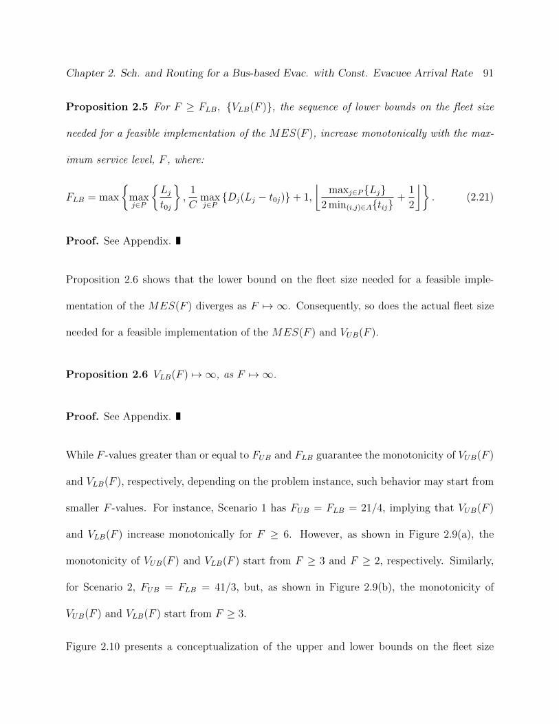
Chapter 2. Sch. and Routing for a Bus-based Evac. with Const. Evacuee Arrival Rate 91
Proposition 2.5 For F ≥ FLB, {VLB(F )}, the sequence of lower bounds on the fleet size
needed for a feasible implementation of the MES(F ), increase monotonically with the max-
imum service level, F , where:
FLB = max
{maxj∈P
{Ljt0j
},
1
Cmaxj∈P{Dj(Lj − t0j)}+ 1,
⌊maxj∈P{Lj}
2 min(i,j)∈A{tij}+
1
2
⌋}. (2.21)
Proof. See Appendix.
Proposition 2.6 shows that the lower bound on the fleet size needed for a feasible imple-
mentation of the MES(F ) diverges as F 7→ ∞. Consequently, so does the actual fleet size
needed for a feasible implementation of the MES(F ) and VUB(F ).
Proposition 2.6 VLB(F ) 7→ ∞, as F 7→ ∞.
Proof. See Appendix.
While F -values greater than or equal to FUB and FLB guarantee the monotonicity of VUB(F )
and VLB(F ), respectively, depending on the problem instance, such behavior may start from
smaller F -values. For instance, Scenario 1 has FUB = FLB = 21/4, implying that VUB(F )
and VLB(F ) increase monotonically for F ≥ 6. However, as shown in Figure 2.9(a), the
monotonicity of VUB(F ) and VLB(F ) start from F ≥ 3 and F ≥ 2, respectively. Similarly,
for Scenario 2, FUB = FLB = 41/3, but, as shown in Figure 2.9(b), the monotonicity of
VUB(F ) and VLB(F ) start from F ≥ 3.
Figure 2.10 presents a conceptualization of the upper and lower bounds on the fleet size

Chapter 2. Sch. and Routing for a Bus-based Evac. with Const. Evacuee Arrival Rate 92
needed for a feasible implementation of the MES(F ) and the total exposure under the
MES(F ) by maximum service level.
Maximum Service Level (F)
Fleet Size (V)
Exposure
Total Exposure
Figure 2.10: Conceptualization of the upper and lower bounds on the fleet size needed for a
feasible implementation of the MES(F ) and its corresponding total exposure.
As shown in this figure, for a fixed (and sufficiently large) fleet size, V , there exist inte-
gers F ∗UB(V ) and F ∗LB(V ) corresponding, respectively, to the largest and smallest F -values
satisfying VUB(F ∗UB(V )) = VLB(F ∗LB(V )) = V , that is:
F ∗UB(V ) = sup{F ∈ N ∧ F ≥ FUB : VUB(F ) ≤ V }, and (2.22)
F ∗LB(V ) = inf{F ∈ N ∧ F ≥ FLB : VLB(F ) ≥ V }. (2.23)
Consequently, F ∗UB(V ) and F ∗LB(V ) + 1 represent, respectively, the largest known F -value
Chapter 2. Sch. and Routing for a Bus-based Evac. with Const. Evacuee Arrival Rate 93
for which a feasible MES(F ) is guaranteed and the smallest known F -value for which the
MES(F ) is infeasible (provided the fleet size parameter, V ). The relationship between FUB,
FLB, F ∗UB(V ), and F ∗LB(V ) is stated in Lemma 2.3.
Lemma 2.3 Either FUB ≤ FLB ≤ F ∗UB(V ) ≤ F ∗LB(V ) or FUB ≤ F ∗UB(V ) ≤ FLB ≤ F ∗LB(V ).
Proof. See Appendix.
As aforementioned, the parameters F ∗UB(V ) and F ∗LB(V ) have important planning appli-
cations. First, given a fixed fleet size, V , the maximum service level should equal, at
least, F ∗UB(V ), as the MES(F ∗UB(V )) is always feasible and as the MES(F ) total expo-
sure is quadratic-decreasing with F . Clearly, there exists a point F ′ (where F ∗UB(V ) ≤ F ′ ≤
F ∗LB(V )), such that the MES(F ′) is feasible, but the MES(F ′ + 1) is infeasible. Although
the total exposure either continues to decrease or remains unchanged for F > F ′, if the
MES(F ) is infeasible, any reductions in total exposure from increased F may not be equi-
table across pick-up locations. Following the discussion in Section 2.3.1.1, if the MES(F ) is
not achieved, then it is possible for the exposure from some pick-up nodes to increase even
though the total exposure either decreases or remains unchanged.
As an example, consider Scenario 1 with a fleet size of V = 12 buses. Since the largest
F -value satisfying VUB(F ) = 12 is 6 and the smallest F -value satisfying VLB(F ) = 12 is 19,
it follows that F ∗UB(12) = 6 and F ∗LB(12) = 19. Consequently, for the given fleet size of 12
buses, the MES(6) is feasible, and F should be set no smaller than 6 (for a total exposure
of 232.0). In addition, since the MES(20) is infeasible, setting F to any values larger than

Chapter 2. Sch. and Routing for a Bus-based Evac. with Const. Evacuee Arrival Rate 94
or equal to 20 may result in non-equitable reductions in exposure across pick-up locations
(assuming any is realizable with 12 vehicles). Since the MES(19) total exposure equals
129.4, since the greatest lower bound on exposure for Scenario 1 equals∑
j∈P Djt20j/2 = 90.0,
and giving the diminishing returns in exposure from increased maximum service level, any
improvements in exposure past F = 19 are likely to be small. The exact F ′-value where the
MES(F ′) is feasible, but the MES(F ′+1) is infeasible, unfortunately, can only be identified
by systematically searching for the largest feasible MES(F ) solution among F = 7, · · · , 19.
Next, an upper bound on the fleet size needed for a feasible solution to the BEP-CA is
presented.
2.3.2.5 Upper Bound on the BEP-CA Fleet Size.
Proposition 2.7 presents an analytical upper bound on the fleet size needed for a feasible
solution to the BEP-CA.
Proposition 2.7 The upper bound on the fleet size needed for a feasible solution to the
BEP-CA, V ∗UB(F ), is calculated as follows:
V ∗UB(F ) = minf=1,··· ,F
{VUB(f)}. (2.24)
Proof. See Appendix.
As aforementioned, while (2.18) is a tight upper bound on the fleet size needed for a feasible
implementation of the MES(F ) in instances where vehicles are dedicated to a single pick-up
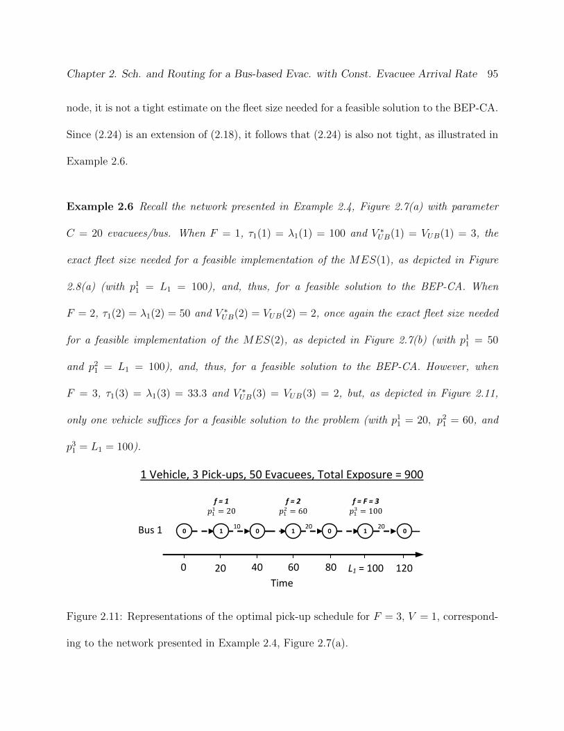
Chapter 2. Sch. and Routing for a Bus-based Evac. with Const. Evacuee Arrival Rate 95
node, it is not a tight estimate on the fleet size needed for a feasible solution to the BEP-CA.
Since (2.24) is an extension of (2.18), it follows that (2.24) is also not tight, as illustrated in
Example 2.6.
Example 2.6 Recall the network presented in Example 2.4, Figure 2.7(a) with parameter
C = 20 evacuees/bus. When F = 1, τ1(1) = λ1(1) = 100 and V ∗UB(1) = VUB(1) = 3, the
exact fleet size needed for a feasible implementation of the MES(1), as depicted in Figure
2.8(a) (with p11 = L1 = 100), and, thus, for a feasible solution to the BEP-CA. When
F = 2, τ1(2) = λ1(2) = 50 and V ∗UB(2) = VUB(2) = 2, once again the exact fleet size needed
for a feasible implementation of the MES(2), as depicted in Figure 2.7(b) (with p11 = 50
and p21 = L1 = 100), and, thus, for a feasible solution to the BEP-CA. However, when
F = 3, τ1(3) = λ1(3) = 33.3 and V ∗UB(3) = VUB(3) = 2, but, as depicted in Figure 2.11,
only one vehicle suffices for a feasible solution to the problem (with p11 = 20, p2
1 = 60, and
p31 = L1 = 100).
Time
120 20 40 60 0 80 L1 = 100
1 Vehicle, 3 Pick-ups, 50 Evacuees, Total Exposure = 900
f = 1
f = 2
f = F = 3
Bus 1 0 1 0 1 0 0 1 10 20 20
Figure 2.11: Representations of the optimal pick-up schedule for F = 3, V = 1, correspond-
ing to the network presented in Example 2.4, Figure 2.7(a).

Chapter 2. Sch. and Routing for a Bus-based Evac. with Const. Evacuee Arrival Rate 96
Corollary 2.3, based on the analytical upper bound introduced in Proposition 2.7, presents
a sufficient condition for the feasibility of the BEP-CA.
Corollary 2.3 Provided the necessary condition for feasibility presented in Lemma 2.2, a
feasible solution to the BEP-CA can always be obtained with∑
j∈P dDjLj/Ce or fewer vehi-
cles.
Proof. See Appendix.
Next, a lower bound on the fleet size needed for a feasible solution to the problem is presented.
2.3.2.6 Lower Bound on the BEP-CA Fleet Size.
Archetti and Speranza (2012); Cordeau and Laporte (2006); Friedrich (2006); Letchford and
Salazar-Gonzalez (2006) and Stray (2010) propose d∑j∈P Qj/Ce, as an analytical lower
bound on the fleet size needed for a feasible solution to the VRP with split deliveries, where
Qj denotes the total demand of pick-up node j (i.e., Qj = DjLj, ∀ j ∈ P ). However, no
literature suggesting a lower bound on the fleet size needed for a feasible solution to the VRP
with split deliveries, service choice, and multiple tours per vehicle was located. Equation
(2.25) presents one such bound:
V ∗LB(F ) =
⌈∑
j∈P
DjLjCbT (F )/2c
⌉, (2.25)
where bT (F )/2c is a proxy for the maximum number of times a vehicle can leave the depot.
Consequently, this lower bound is similar to the one presented in the literature, except that

Chapter 2. Sch. and Routing for a Bus-based Evac. with Const. Evacuee Arrival Rate 97
it also accounts for the possibility of multiple tours per vehicle. Corollary 2.4 presents a
greatest lower bound on the fleet size needed for a feasible solution to the BEP-CA, that is,
one that does not depend on the maximum service level.
Corollary 2.4 A feasible solution to the BEP-CA (provided one exists) always demands
⌈ ∑j∈P DjLj
Cb(θ + 1)/2c
⌉,
or more vehicles, where θ = maxj∈P{Lj}/min(i,j)∈A{tij}.
Proof. See Appendix.
Figure 2.12 depicts the upper and lower bounds on the fleet size needed for a feasible solution
to the BEP-CA and the fleet size obtained by (2.17) by maximum service level for Scenarios
1 and 2 (Figures 2.12(a) and 2.12(b), respectively).
0
2
4
6
8
10
1 2 3 4 5 6 7 8 9 10
Fle
et
Size
(Sc
en
ari
o 1
)
Maximum Service Level (F)
UB on the Fleet Size for a Feasible Solution
LB on the Fleet Size for a Feasible Solution
Actual Fleet Size for a Feasible Solution
0
2
4
6
8
10
1 2 3 4 5 6 7 8 9 10
Fle
et
Size
(Sc
en
ari
o 2
)
Maximum Service Level (F)
UB on the Fleet Size for a Feasible Solution
LB on the Fleet Size for a Feasible Solution
Actual Fleet Size for a Feasible Solution
(a) (b)
Figure 2.12: Upper bound, lower bound, and the exact fleet size needed for a feasible solution
to the problem by the maximum service level for Scenarios 1 (a) and 2 (b).
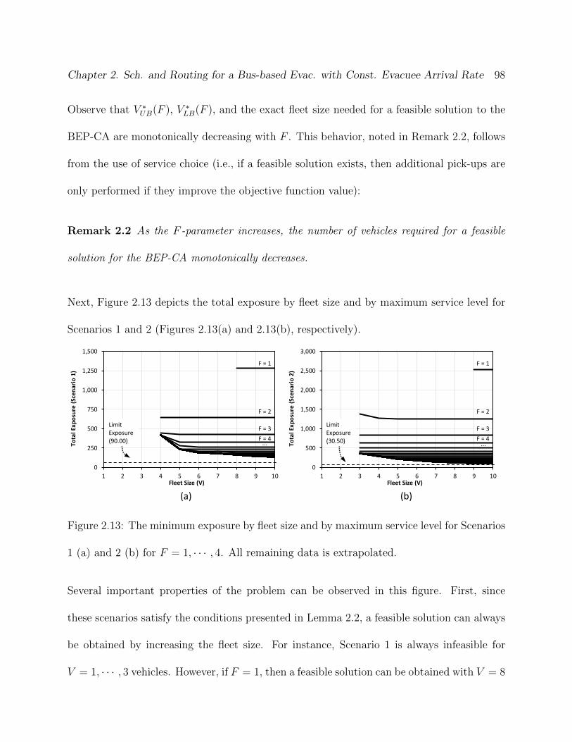
Chapter 2. Sch. and Routing for a Bus-based Evac. with Const. Evacuee Arrival Rate 98
Observe that V ∗UB(F ), V ∗LB(F ), and the exact fleet size needed for a feasible solution to the
BEP-CA are monotonically decreasing with F . This behavior, noted in Remark 2.2, follows
from the use of service choice (i.e., if a feasible solution exists, then additional pick-ups are
only performed if they improve the objective function value):
Remark 2.2 As the F -parameter increases, the number of vehicles required for a feasible
solution for the BEP-CA monotonically decreases.
Next, Figure 2.13 depicts the total exposure by fleet size and by maximum service level for
Scenarios 1 and 2 (Figures 2.13(a) and 2.13(b), respectively).
0
250
500
750
1,000
1,250
1,500
1 2 3 4 5 6 7 8 9 10
To
tal E
xpo
sure
(Sc
en
ari
o 1
)
Fleet Size (V)
F = 1
F = 2
F = 3
F = 4
Limit Exposure (90.00) ...
0
500
1,000
1,500
2,000
2,500
3,000
1 2 3 4 5 6 7 8 9 10
To
tal E
xpo
sure
(Sc
en
ari
o 2
)
Fleet Size (V)
F = 1
F = 2
F = 3
F = 4 ...
Limit Exposure (30.50)
(a) (b)
Figure 2.13: The minimum exposure by fleet size and by maximum service level for Scenarios
1 (a) and 2 (b) for F = 1, · · · , 4. All remaining data is extrapolated.
Several important properties of the problem can be observed in this figure. First, since
these scenarios satisfy the conditions presented in Lemma 2.2, a feasible solution can always
be obtained by increasing the fleet size. For instance, Scenario 1 is always infeasible for
V = 1, · · · , 3 vehicles. However, if F = 1, then a feasible solution can be obtained with V = 8

Chapter 2. Sch. and Routing for a Bus-based Evac. with Const. Evacuee Arrival Rate 99
vehicles, and if F ≥ 2, then a feasible solution can be obtained with V = 4 vehicles. Similarly,
Scenario 2 is always infeasible for V = 1 and V = 2 vehicles. However, if F = 1 then a
feasible solution can be obtained with V = 9 vehicles, and if F ≥ 2, then a feasible solution
can be obtained with V = 3 vehicles. These results are also apparent from Figures 2.9 and
2.12. Second, the MES(F ) is feasible for a sufficiently large fleet size, but increasing the fleet
size beyond the number of vehicles required for a feasible MES(F ) does not improve the
objective function value (i.e., the level curves becomes flat for a sufficiently large fleet). Third,
since the BEP-CA constraint set does not require all pick-ups to be performed, the contour
lines depicted in Figure 2.13 are monotonically decreasing and never cross. Consequently,
if a feasible solution exists, then the total exposure can be reduced by either increasing the
maximum service level, the fleet size (although not beyond the fleet size needed for a feasible
implementation of the MES(F )), or both. In every case, the objective function value will
remain between the total exposure for the previous solution and the one corresponding to
the MES(F ) for the new F -parameter. Moreover, note that as F increases, the contour
lines approach each other, indicating the diminishing returns from increased F , and that the
total exposure converges to the sum of accumulated exposures for the first pick-up at each
pick-up node,∑
j∈P{Djt20j/2}. Lastly, observe that while the fleet size needed for a feasible
implementation of the MES(F ) first increased and later decreased with F , the one required
for a feasible solution to the BEP-CA monotonically decreased. The next section presents
and examines a formulation and an upper bound on the maximum number of arc traversals
per vehicle for a given F -parameter, T (F ).

Chapter 2. Sch. and Routing for a Bus-based Evac. with Const. Evacuee Arrival Rate 100
2.3.3 Upper Bound on the Maximum Number of Arc Traversals
per Vehicle
While T (F ), the maximum number of arc traversals per vehicle for a given F -parameter, is
not based on a policy decision, it may affect the model performance and results, as excessive
values increase the complexity of the model, while insufficient values may either prevent its
feasibility or yield suboptimal solutions. The following mixed-integer formulation identifies
T (F ). The decision variables, objective function, and constraint set for this MIP are as
follows:
Table 2.2: Decision variables for the T (F ) MIP.
Variable Description
xtij binary variable that equals 1 if arc (i, j) is the tth arc traversed by the vehicle,
else 0, ∀ (i, j) ∈ A, t = 1, · · · , T , where T is a large positive integer (i.e.,
T � T (F )).
dt time when the vehicle finishes the tth arc traversal. Let d0 = 0, ∀ t = 0, · · · , T
T (F ) Formulation:
Maximize T (F ) =∑
(i,j)∈A
T∑
t=1
xtij (2.26)
subject to
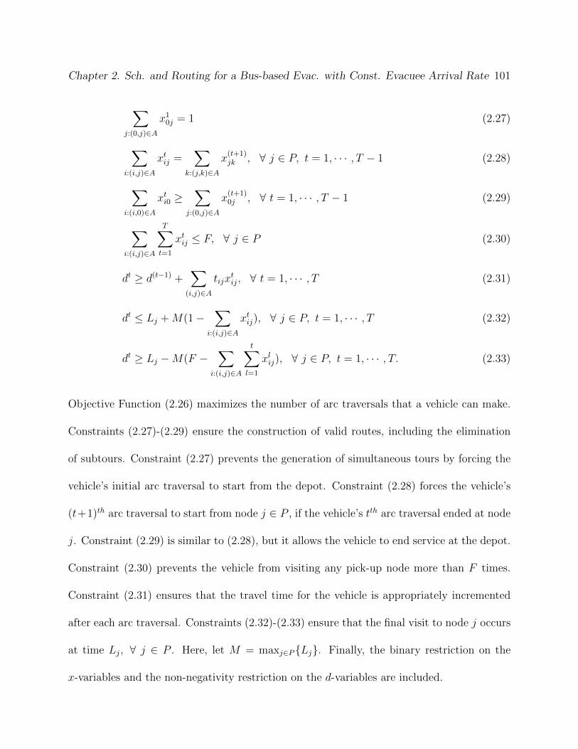
Chapter 2. Sch. and Routing for a Bus-based Evac. with Const. Evacuee Arrival Rate 101
∑
j:(0,j)∈A
x10j = 1 (2.27)
∑
i:(i,j)∈A
xtij =∑
k:(j,k)∈A
x(t+1)jk , ∀ j ∈ P, t = 1, · · · , T − 1 (2.28)
∑
i:(i,0)∈A
xti0 ≥∑
j:(0,j)∈A
x(t+1)0j , ∀ t = 1, · · · , T − 1 (2.29)
∑
i:(i,j)∈A
T∑
t=1
xtij ≤ F, ∀ j ∈ P (2.30)
dt ≥ d(t−1) +∑
(i,j)∈A
tijxtij, ∀ t = 1, · · · , T (2.31)
dt ≤ Lj +M(1−∑
i:(i,j)∈A
xtij), ∀ j ∈ P, t = 1, · · · , T (2.32)
dt ≥ Lj −M(F −∑
i:(i,j)∈A
t∑
l=1
xlij), ∀ j ∈ P, t = 1, · · · , T. (2.33)
Objective Function (2.26) maximizes the number of arc traversals that a vehicle can make.
Constraints (2.27)-(2.29) ensure the construction of valid routes, including the elimination
of subtours. Constraint (2.27) prevents the generation of simultaneous tours by forcing the
vehicle’s initial arc traversal to start from the depot. Constraint (2.28) forces the vehicle’s
(t+1)th arc traversal to start from node j ∈ P , if the vehicle’s tth arc traversal ended at node
j. Constraint (2.29) is similar to (2.28), but it allows the vehicle to end service at the depot.
Constraint (2.30) prevents the vehicle from visiting any pick-up node more than F times.
Constraint (2.31) ensures that the travel time for the vehicle is appropriately incremented
after each arc traversal. Constraints (2.32)-(2.33) ensure that the final visit to node j occurs
at time Lj, ∀ j ∈ P . Here, let M = maxj∈P{Lj}. Finally, the binary restriction on the
x-variables and the non-negativity restriction on the d-variables are included.
Chapter 2. Sch. and Routing for a Bus-based Evac. with Const. Evacuee Arrival Rate 102
Since this formulation does not require the use of both binary and continuous variables to
track the flow of multiple vehicles and evacuees through the network, it has much lower
dimensionality than the BEP-CA, and, thus, is easier to solve. Nonetheless, the following
greedy algorithm is shown to provide an upper bound on T (F ) in polynomial time:
1. Set L = P , F ∗ = 0, and t∗ = min(i,j)∈A{tij};
2. While L 6= {∅}:
(a) Set j∗ = arg minj∈L{Lj};
(b) Set F ∗ = min{bLj∗/2t∗ + 1/2c, F + F ∗};
(c) Set L = L/j∗;
3. Set TUB(F ) = 2F ∗,
where L denotes the set of unexplored pick-up nodes and F ∗ denotes the number of pick-
ups performed on previously explored pick-up nodes. In summary, this procedure identifies
the maximum number of arc traversals per vehicle possible such that neither the maximum
service level nor the last pick-up times are violated. Since complete graphs have |A| =
|N |(|N | − 1)/2 arcs, the execution of this procedure is bounded by a polynomial of order
O(|N |2), and, thus, is easier to solve than the corresponding MIP, which is combinatorial
in nature. However, since this upper bound procedure assumes the smallest arc traversal
time between nodes, depending on the problem instance, it can substantially overestimate
the number of arc traversals per vehicle.

Chapter 2. Sch. and Routing for a Bus-based Evac. with Const. Evacuee Arrival Rate 103
As an example of the algorithm, consider the network from Scenario 1, with F = 3.
1. Initialization: Set L = {1, 2, 3}, F ∗ = 0, and t∗ = 4;
2. Iteration 1: Set j∗ = {1}, F ∗ = min{bL1/8 + 1/2c, 3 + 0} = 2, and L = {2, 3};
3. Iteration 2: Set j∗ = {3}, F ∗ = min{bL3/8 + 1/2c, 3 + 2} = 3, and L = {2};
4. Iteration 3: Set j∗ = {2}, F ∗ = min{bL2/8 + 1/2c, 3 + 3} = 3, and L = {∅};
5. Termination criteria met (L = {∅}). Return TUB(F ) = 6 arc traversals.
Figure 2.14 depicts the results obtained from the MIP formulation, from the proposed upper
bound procedure, and the minimum T (F )-parameter needed for a feasible implementation
of the MES(F ) by the maximum service level for Scenarios 1 and 2 (Figures 2.14(a) and
2.14(b), respectively).
Observe that the minimum T (F )-parameter needed a feasible implementation of the
MES(F ) oscillates as the F -parameter increases. Most likely, this non-monotonic behavior
follows from the concurrent increase in fleet size, as every increment in the V -parameter
lessens the number of arc traversals that each vehicle needs to perform in order to accommo-
date all pick-ups. Conversely, the maximum number of arc traversals per vehicle obtained
from the MIP formulation presented in Section 2.2 and from the proposed upper bound
procedure increase monotonically with F , thus leading to Remarks 2.3 and 2.4:
Remark 2.3 The minimum T (F )-parameter needed for a feasible implementation of the
MES(F ) may not increase monotonically with F .
Chapter 2. Sch. and Routing for a Bus-based Evac. with Const. Evacuee Arrival Rate 104
0
1
2
3
4
5
6
7
1 2 3 4 5 6 7 8 9 10
Max
imu
m N
um
ber
of
Arc
Tra
vers
als
per
Veh
icle
(Sc
enar
io 1
)
Maximum Service Level (F)
T(F) from UB Procedure
T(F) from MIP
Minimum T(F) for a Feasible MES(F)0
2
4
6
8
10
12
14
16
1 2 3 4 5 6 7 8 9 10
Max
imu
m N
um
ber
of
Arc
Tra
vers
als
per
Veh
icle
(Sc
enar
io 2
)
Maximum Service Level (F)
T(F) from UB Procedure
T(F) from MIP
Minimum T(F) for a Feasible MES(F)
(a) (b)
Figure 2.14: T (F ), as obtained from the MIP formulation, from the upper bound procedure,
and the minimum value needed for a feasible implementation of the MES(F ) by maximum
service level for Scenarios 1 (a) and 2 (b).
Remark 2.4 The T (F )-parameter obtained from the MIP formulation presented in Section
2.2 and the upper bound procedure presented in this section increase monotonically with F .
The next section summarizes the findings of this paper and lists directions for future research.
2.4 Conclusions and Further Research
This paper introduced the Bus Evacuation Problem with Constant Evacuee Arrival Rate
(BEP-CA), a variant of the vehicle routing problem adapted for bus-based, regional evac-
uation planning. Several important properties of the model were identified. In particular,
the effect of maximum service level (i.e., the maximum number of pick-ups allowed on each
pick-up location) and fleet size over the problem feasibility and the total exposure objective

Chapter 2. Sch. and Routing for a Bus-based Evac. with Const. Evacuee Arrival Rate 105
function value was examined. It was shown that, under a necessary condition for feasibility,
if a feasible solution does not exist, then one can be obtained by increasing the fleet size;
that if one exists, then the exposure can be reduced by either increasing the fleet size or the
maximum service level; and that, after the MES(F ) is attained, the exposure can only be
reduced by further increasing the maximum service level, but with diminishing returns. In
addition, upper and lower bounds on the fleet size required for feasibility and for such bound
on exposure, and an exact formulation and an upper bound on the maximum number of arc
traversals per vehicle were proposed. More importantly, it was shown that, depending on
the problem instance, it is possible to reduce both the fleet size requirement and the total
exposure objective function, and that past a certain threshold, there is an optimal choice for
the maximum service level (or a range of potential values, if the problem cannot be solved
to optimality) that guarantees an efficient usage of the available fleet and equitable reduc-
tions in exposure across pick-up locations. Despite these advances, the literature focusing
on bus-based evacuation is scarce and considerable research is warranted. First, while the
assumption of a constant arrival rate presents an important distinction from the current
literature on transit-based evacuation, it is still unrealistically portraying evacuee arrival
behavior, as the true arrival process is probabilistic and will likely vary over time. Moreover,
obtaining an optimal solution is computationally expensive. Therefore, before the BEP-CA
can be implemented in networks of practical size, alternative solution methodologies, such
as problem decomposition and use of metaheuristics, should be studied.
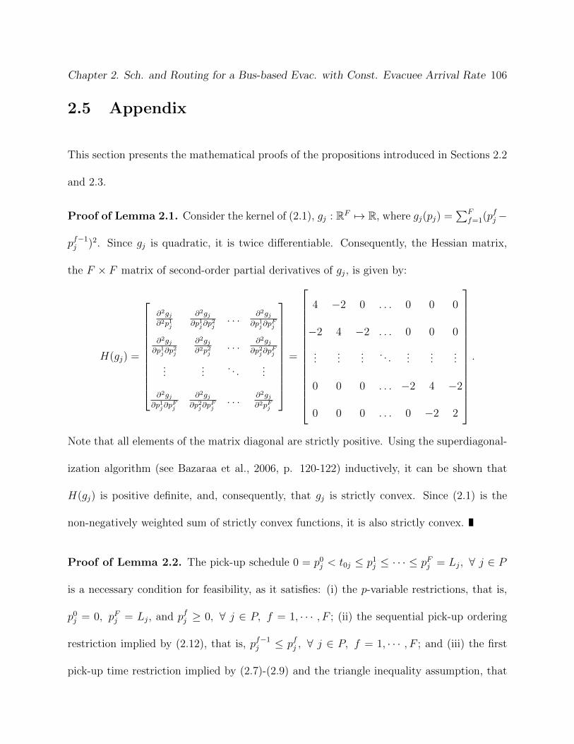
Chapter 2. Sch. and Routing for a Bus-based Evac. with Const. Evacuee Arrival Rate 106
2.5 Appendix
This section presents the mathematical proofs of the propositions introduced in Sections 2.2
and 2.3.
Proof of Lemma 2.1. Consider the kernel of (2.1), gj : RF 7→ R, where gj(pj) =∑F
f=1(pfj−
pf−1j )2. Since gj is quadratic, it is twice differentiable. Consequently, the Hessian matrix,
the F × F matrix of second-order partial derivatives of gj, is given by:
H(gj) =
∂2gj∂2p1j
∂2gj∂p1j∂p
2j
. . .∂2gj
∂p1j∂pFj
∂2gj∂p1j∂p
2j
∂2gj∂2p2j
. . .∂2gj
∂p2j∂pFj
......
. . ....
∂2gj∂p1j∂p
Fj
∂2gj∂p2j∂p
Fj
. . .∂2gj∂2pFj
=
4 −2 0 . . . 0 0 0
−2 4 −2 . . . 0 0 0
......
.... . .
......
...
0 0 0 . . . −2 4 −2
0 0 0 . . . 0 −2 2
.
Note that all elements of the matrix diagonal are strictly positive. Using the superdiagonal-
ization algorithm (see Bazaraa et al., 2006, p. 120-122) inductively, it can be shown that
H(gj) is positive definite, and, consequently, that gj is strictly convex. Since (2.1) is the
non-negatively weighted sum of strictly convex functions, it is also strictly convex.
Proof of Lemma 2.2. The pick-up schedule 0 = p0j < t0j ≤ p1
j ≤ · · · ≤ pFj = Lj, ∀ j ∈ P
is a necessary condition for feasibility, as it satisfies: (i) the p-variable restrictions, that is,
p0j = 0, pFj = Lj, and pfj ≥ 0, ∀ j ∈ P, f = 1, · · · , F ; (ii) the sequential pick-up ordering
restriction implied by (2.12), that is, pf−1j ≤ pfj , ∀ j ∈ P, f = 1, · · · , F ; and (iii) the first
pick-up time restriction implied by (2.7)-(2.9) and the triangle inequality assumption, that
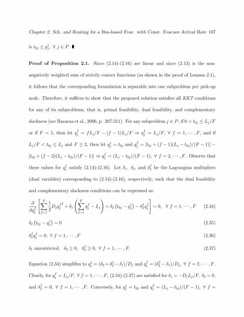
Chapter 2. Sch. and Routing for a Bus-based Evac. with Const. Evacuee Arrival Rate 107
is t0j ≤ p1j , ∀ j ∈ P .
Proof of Proposition 2.1. Since (2.14)-(2.16) are linear and since (2.13) is the non-
negatively weighted sum of strictly convex functions (as shown in the proof of Lemma 2.1),
it follows that the corresponding formulation is separable into one subproblem per pick-up
node. Therefore, it suffices to show that the proposed solution satisfies all KKT conditions
for any of its subproblems, that is, primal feasibility, dual feasibility, and complementary
slackness (see Bazaraa et al., 2006, p. 207-211). For any subproblem j ∈ P , if 0 < t0j ≤ Lj/F
or if F = 1, then let qfj = fLj/F − (f − 1)Lj/F ⇒ qfj = Lj/F, ∀ f = 1, · · · , F , and if
Lj/F < t0j ≤ Lj and F ≥ 2, then let q1j = t0j and qfj = [t0j + (f − 1)(Lj − t0j)/(F − 1)] −
[t0j + (f − 2)(Lj − t0j)/(F − 1)] ⇒ qfj = (Lj − t0j)/(F − 1), ∀ f = 2, · · · , F . Observe that
these values for qfj satisfy (2.14)-(2.16). Let δ1, δ2, and δf3 be the Lagrangian multipliers
(dual variables) corresponding to (2.14)-(2.16), respectively, such that the dual feasibility
and complementary slackness conditions can be expressed as:
∂
∂qfj
[F∑
f=1
1
2Djq
fj
2+ δ1
(F∑
f=1
qfj − Lj)
+ δ2
(t0j − q1
j
)− δf3 qfj
]= 0, ∀ f = 1, · · · , F (2.34)
δ2
(t0j − q1
j
)= 0 (2.35)
δf3 qfj = 0, ∀ f = 1, · · · , F (2.36)
δ1 unrestricted, δ2 ≥ 0, δf3 ≥ 0, ∀ f = 1, · · · , F. (2.37)
Equation (2.34) simplifies to q1j = (δ2 + δ1
3 − δ1)/Dj and qfj = (δf3 − δ1)/Dj, ∀ f = 2, · · · , F .
Clearly, for qfj = Lj/F, ∀ f = 1, · · · , F , (2.34)-(2.37) are satisfied for δ1 = −DjLj/F, δ2 = 0,
and δf3 = 0, ∀ f = 1, · · · , F . Conversely, for q1j = t0j and qfj = (Lj − t0j)/(F − 1), ∀ f =
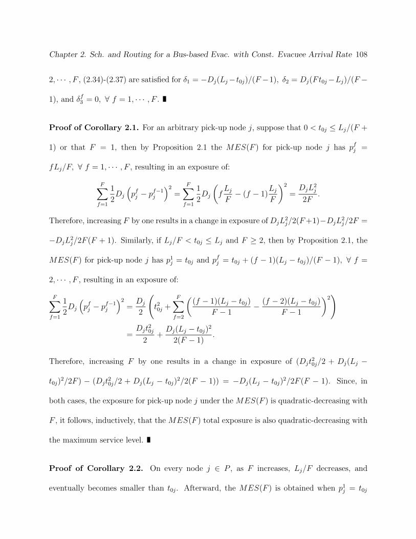
Chapter 2. Sch. and Routing for a Bus-based Evac. with Const. Evacuee Arrival Rate 108
2, · · · , F , (2.34)-(2.37) are satisfied for δ1 = −Dj(Lj−t0j)/(F −1), δ2 = Dj(Ft0j−Lj)/(F −
1), and δf3 = 0, ∀ f = 1, · · · , F .
Proof of Corollary 2.1. For an arbitrary pick-up node j, suppose that 0 < t0j ≤ Lj/(F +
1) or that F = 1, then by Proposition 2.1 the MES(F ) for pick-up node j has pfj =
fLj/F, ∀ f = 1, · · · , F , resulting in an exposure of:
F∑
f=1
1
2Dj
(pfj − pf−1
j
)2
=F∑
f=1
1
2Dj
(fLjF− (f − 1)
LjF
)2
=DjL
2j
2F.
Therefore, increasing F by one results in a change in exposure of DjL2j/2(F+1)−DjL
2j/2F =
−DjL2j/2F (F + 1). Similarly, if Lj/F < t0j ≤ Lj and F ≥ 2, then by Proposition 2.1, the
MES(F ) for pick-up node j has p1j = t0j and pfj = t0j + (f − 1)(Lj − t0j)/(F − 1), ∀ f =
2, · · · , F , resulting in an exposure of:
F∑
f=1
1
2Dj
(pfj − pf−1
j
)2
=Dj
2
(t20j +
F∑
f=2
((f − 1)(Lj − t0j)
F − 1− (f − 2)(Lj − t0j)
F − 1
)2)
=Djt
20j
2+Dj(Lj − t0j)2
2(F − 1).
Therefore, increasing F by one results in a change in exposure of (Djt20j/2 + Dj(Lj −
t0j)2/2F ) − (Djt
20j/2 + Dj(Lj − t0j)
2/2(F − 1)) = −Dj(Lj − t0j)2/2F (F − 1). Since, in
both cases, the exposure for pick-up node j under the MES(F ) is quadratic-decreasing with
F , it follows, inductively, that the MES(F ) total exposure is also quadratic-decreasing with
the maximum service level.
Proof of Corollary 2.2. On every node j ∈ P , as F increases, Lj/F decreases, and
eventually becomes smaller than t0j. Afterward, the MES(F ) is obtained when p1j = t0j
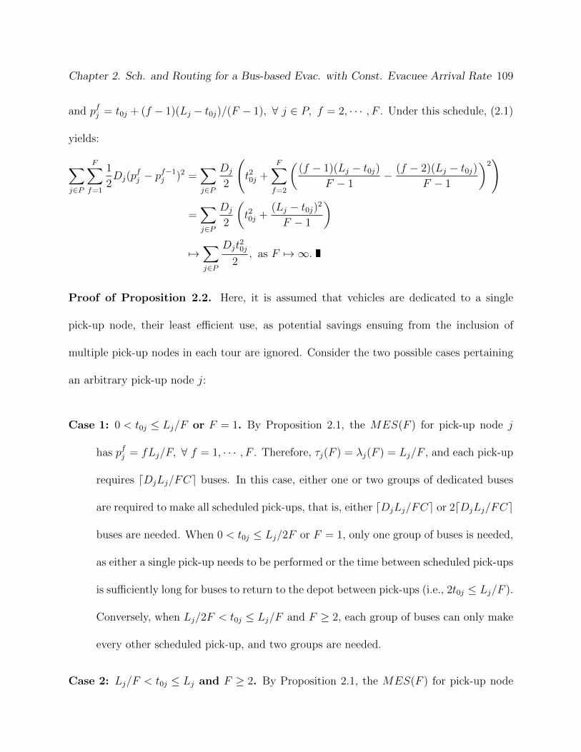
Chapter 2. Sch. and Routing for a Bus-based Evac. with Const. Evacuee Arrival Rate 109
and pfj = t0j + (f − 1)(Lj − t0j)/(F − 1), ∀ j ∈ P, f = 2, · · · , F . Under this schedule, (2.1)
yields:
∑
j∈P
F∑
f=1
1
2Dj(p
fj − pf−1
j )2 =∑
j∈P
Dj
2
(t20j +
F∑
f=2
((f − 1)(Lj − t0j)
F − 1− (f − 2)(Lj − t0j)
F − 1
)2)
=∑
j∈P
Dj
2
(t20j +
(Lj − t0j)2
F − 1
)
7→∑
j∈P
Djt20j
2, as F 7→ ∞.
Proof of Proposition 2.2. Here, it is assumed that vehicles are dedicated to a single
pick-up node, their least efficient use, as potential savings ensuing from the inclusion of
multiple pick-up nodes in each tour are ignored. Consider the two possible cases pertaining
an arbitrary pick-up node j:
Case 1: 0 < t0j ≤ Lj/F or F = 1. By Proposition 2.1, the MES(F ) for pick-up node j
has pfj = fLj/F, ∀ f = 1, · · · , F . Therefore, τj(F ) = λj(F ) = Lj/F , and each pick-up
requires dDjLj/FCe buses. In this case, either one or two groups of dedicated buses
are required to make all scheduled pick-ups, that is, either dDjLj/FCe or 2dDjLj/FCe
buses are needed. When 0 < t0j ≤ Lj/2F or F = 1, only one group of buses is needed,
as either a single pick-up needs to be performed or the time between scheduled pick-ups
is sufficiently long for buses to return to the depot between pick-ups (i.e., 2t0j ≤ Lj/F ).
Conversely, when Lj/2F < t0j ≤ Lj/F and F ≥ 2, each group of buses can only make
every other scheduled pick-up, and two groups are needed.
Case 2: Lj/F < t0j ≤ Lj and F ≥ 2. By Proposition 2.1, the MES(F ) for pick-up node

Chapter 2. Sch. and Routing for a Bus-based Evac. with Const. Evacuee Arrival Rate 110
j has p1j = t0j and pfj = t0j + (f − 1)(Lj − t0j)/(F − 1), ∀ f = 2, · · · , F . Therefore,
τj(F ) = (Lj−t0j)/(F−1), λj(F ) = t0j, the first pick-up requires dDjt0j/Ce buses, and
each subsequent pick-up requires dDj(Lj − t0j)/(F − 1)Ce buses. Under this pick-up
schedule, vehicles also do not have time to return to the depot between pick-ups, and
multiple groups of buses are needed. Specifically, this pick-up schedule requires a total
of dDjt0j/Ce+(min{d2t0j(F −1)/(Lj− t0j)e, F}−1)dDj(Lj− t0j)/(F −1)Ce vehicles,
where min{d2t0j(F − 1)/(Lj − t0j)e, F} is the total number of groups of buses needed,
namely the minimum between the ceiling of the round-trip time to node j divided by
the interval between scheduled pick-up times, and F , an upper bound on the number
of groups assuming that each group visits node j at least once.
In both cases, (2.18) corresponds to the exact number of vehicles required for a feasible
implementation of the MES(F ) on pick-up node j, and, inductively, for the MES(F ).
Proof of Proposition 2.3. First, note that T (F )− 1 is as an upper bound on the number
of pick-ups per vehicle, assuming that each vehicle performs a single tour with a single
returning arc to the depot. Second, F |P | is the total number of distinct scheduled pick-up
times under the MES(F ). Consequently, VLB(F ) corresponds to the product of two factors:
a lower bound on the number of groups of buses simultaneously performing pick-ups under
the MES(F ) and a lower bound on the number of buses needed in each group in order to
pick-up all evacuees that arrived between scheduled pick-up times.
Proof of Proposition 2.4. Let F ≥ FUB. Since F ≥ Lj/t0j, ∀ j ∈ P , it follows that for
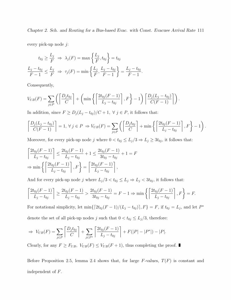
Chapter 2. Sch. and Routing for a Bus-based Evac. with Const. Evacuee Arrival Rate 111
every pick-up node j:
t0j ≥LjF⇒ λj(F ) = max
{LjF, t0j
}= t0j
Lj − t0jF − 1
≤ LjF⇒ τj(F ) = min
{LjF,Lj − t0jF − 1
}=Lj − t0jF − 1
.
Consequently,
VUB(F ) =∑
j∈P
(⌈Djt0jC
⌉+
(min
{⌈2t0j(F − 1)
Lj − t0j
⌉, F
}− 1
)⌈Dj(Lj − t0j)C(F − 1)
⌉).
In addition, since F ≥ Dj(Lj − t0j)/C + 1, ∀ j ∈ P , it follows that:
⌈Dj(Lj − t0j)C(F − 1)
⌉= 1, ∀ j ∈ P ⇒ VUB(F ) =
∑
j∈P
(⌈Djt0jC
⌉+ min
{⌈2t0j(F − 1)
Lj − t0j
⌉, F
}− 1
).
Moreover, for every pick-up node j where 0 < t0j ≤ Lj/3⇒ Lj ≥ 3t0j, it follows that:
⌈2t0j(F − 1)
Lj − t0j
⌉≤ 2t0j(F − 1)
Lj − t0j+ 1 ≤ 2t0j(F − 1)
3t0j − t0j+ 1 = F
⇒ min
{⌈2t0j(F − 1)
Lj − t0j
⌉, F
}=
⌈2t0j(F − 1)
Lj − t0j
⌉,
And for every pick-up node j where Lj/3 < t0j ≤ Lj ⇒ Lj < 3t0j, it follows that:
⌈2t0j(F − 1)
Lj − t0j
⌉≥ 2t0j(F − 1)
Lj − t0j>
2t0j(F − 1)
3t0j − t0j= F − 1⇒ min
{⌈2t0j(F − 1)
Lj − t0j
⌉, F
}= F.
For notational simplicity, let min{d2t0j(F − 1)/(Lj − t0j)e, F} = F , if t0j = Lj, and let P ∗
denote the set of all pick-up nodes j such that 0 < t0j ≤ Lj/3, therefore:
⇒ VUB(F ) =∑
j∈P
⌈Djt0jC
⌉+∑
j∈P ∗
⌈2t0j(F − 1)
Lj − t0j
⌉+ F (|P | − |P ∗|)− |P |.
Clearly, for any F ≥ FUB, VUB(F ) ≤ VUB(F + 1), thus completing the proof.
Before Proposition 2.5, lemma 2.4 shows that, for large F -values, T (F ) is constant and
independent of F .

Chapter 2. Sch. and Routing for a Bus-based Evac. with Const. Evacuee Arrival Rate 112
Lemma 2.4 If F ≥ b(θ + 1)/2c, then T (F ) = φ, a constant independent of F , such that
φ ≤ 2b(θ + 1)/2c and
θ =maxj∈P{Lj}
min(i,j)∈A{tij}.
Proof. First, observe that F ≥ b(θ + 1)/2c ⇒ F ≥ b(Lj + t∗)/2t∗c, ∀ j ∈ P , where
t∗ = min(i,j)∈A{tij}. Consequently, step 2(b) of the upper bound procedure on T (F ) reduces
to F ∗ = b(Lj∗ + t∗)/2t∗c. Since the algorithm assesses nodes from shortest to longest
evacuation end-times, on the last iteration, F ∗ = b(maxj∈P{Lj} + t∗)/2t∗c = b(θ + 1)/2c,
and since TUB(F ) = 2F ∗, it follows that T (F ) = φ, where φ is a constant independent of F
and φ ≤ 2b(θ + 1)/2c.
Proof of Proposition 2.5. Let F ≥ FLB. Since F ≥ Lj/t0j, ∀ j ∈ P , it follows that for
every pick-up node j:
Lj − t0jF − 1
≤ LjF⇒ τj(F ) = min
{LjF,Lj − t0jF − 1
}=Lj − t0jF − 1
⇒ VLB(F ) =
⌈F |P |
T (F )− 1
⌉minj∈P
{⌈Dj(Lj − t0j)C(F − 1)
⌉}.
In addition, since F ≥ Dj(Lj − t0j)/C + 1, ∀ j ∈ P , it follows that:
⌈Dj(Lj − t0j)C(F − 1)
⌉= 1, ∀ j ∈ P ⇒ VLB(F ) =
⌈F |P |
T (F )− 1
⌉.
Finally, since F ≥ b(θ + 1)/2c, by Proposition 2.4, T (F ) = φ, where φ is a constant inde-
pendent of F and φ ≤ 2b(θ + 1)/2c, consequently:
VLB(F ) =
⌈F |P |φ− 1
⌉.

Chapter 2. Sch. and Routing for a Bus-based Evac. with Const. Evacuee Arrival Rate 113
Clearly, for any F ≥ FLB, VLB(F ) ≤ VLB(F + 1), thus completing the proof.
Proof of Proposition 2.6. Here, it is shown that 6 ∃M ∈ R such that VLB(F ) < M, ∀ F ∈
N. Let M ∈ R be given, and let F ≥ F ∗(M), where:
F ∗(M) = max
{FLB,
2Mb(θ + 1)/2c|P |
}.
Since F ≥ FLB, it follows, from the proof of Proposition 2.5, that:
VLB(F ) =
⌈F |P |φ− 1
⌉⇒ VLB(F ) ≥
⌈F |P |
2b(θ + 1)/2c
⌉, as φ ≤ 2b(θ + 1)/2c.
In addition, since F ≥ 2Mb(θ + 1)/2c/|P |, it follows that VLB(F ) ≥ dMe ≥ M . Since for
every arbitrary real number M , there exists a real number F ∗(M), such that F ≥ F ∗(M)
implies that VLB(F ) ≥M , and since, by Proposition 2.5, the sequence of lower bounds on the
fleet size needed for a feasible implementation of the MES(F ) is monotonically increasing
for F ≥ FLB, it follows that VLB(F ) 7→ ∞, as F 7→ ∞.
Proof of Lemma 2.3. The relationship between FUB, FLB, F ∗UB(V ), and F ∗LB(V ) can
be derived from their definitions. Since VUB(F ) ≥ VLB(F ), ∀ F ∈ N, (2.22)-(2.23) imply
that F ∗UB(V ) ≤ F ∗LB(V ), that FUB ≤ F ∗UB(V ), and that FLB ≤ F ∗LB(V ). Since the term
d(θ + 1)/2e ≥ 0 for θ = maxj∈P{Lj}/min(i,j)∈A{tij}, (2.20)-(2.21) imply that FUB ≤ FLB.
Altogether, either FUB ≤ FLB ≤ F ∗UB(V ) ≤ F ∗LB(V ) or FUB ≤ F ∗UB(V ) ≤ FLB ≤ F ∗LB(V ).
Proof of Proposition 2.7. This bound corresponds to the smallest upper bound on the
fleet size needed for a feasible implementation of the MES(f) for f = 1, · · · , F , and holds
for two reasons. First, since (2.18) is an upper bound on the fleet size needed for a feasible
Chapter 2. Sch. and Routing for a Bus-based Evac. with Const. Evacuee Arrival Rate 114
implementation of the MES(F ), it is also an upper bound on the fleet size needed for a
feasible solution. Second, since the BEP-CA does not require all pick-ups to be performed,
once the fleet size is sufficiently large for a feasible solution, increasing F will never result in
a larger fleet size requirement.
Proof of Corollary 2.3. First, observe that the upper bound on the fleet size needed for
a feasible solution to the BEP-CA is monotonically decreasing with F , as:
minf=1,··· ,F
{VUB(F )} ≥ min{ minf=1,··· ,F
{VUB(F )}, VUB(F + 1)}
= minf=1,··· ,F+1
{VUB(F )}
Consequently, the exact fleet size needed for a feasible solution to the BEP-CA is always
smaller than or equal to VUB(1) =∑
j∈P dDjLj/Ce.
Proof of Corollary 2.4. Since T (F ) is monotonically increasing with F , the lower bound
on the fleet size needed for a feasible solution to the BEP-CA, V ∗LB(F ), is monotonically
decreasing with F . Moreover, by Proposition 2.4, for F ≥ b(θ+ 1)/2c, T (F ) ≤ 2b(θ+ 1)/2c.
Consequently, the exact fleet size needed for a feasible solution to the BEP-CA is always
greater than or equal to:
d∑
j∈P
DjLj/Cb(θ + 1)/2ce,
where θ = maxj∈P{Lj}/min(i,j)∈A{tij}. Hence completing the proof.
Chapter 3
A Variant of the Ritter Relaxation
Algorithm Applied to Problems with
Mixed-Integer Subproblems and
Linear or Quadratic Objective
Functions
115
Chapter 3. A Variant of the Ritter Relaxation Algorithm Applied to MIQP Problems 116
A Variant of the Ritter Relaxation Algorithm Applied
to Problems with Mixed-Integer Subproblems and
Linear or Quadratic Objective Functions
Victor C. Pereira and Douglas R. Bish
(ABSTRACT)
This research introduces a variation of the Ritter (1967) Relaxation Algorithm able to solve
bordered (or arrowhead) structure problems with linear, integer, or mixed-integer subprob-
lems and with linear or quadratic objective functions without the need to compound multiple
decomposition/relaxation strategies. Empirical studies demonstrate that the proposed algo-
rithm is a viable alternative for solving difficult, bordered-structure, optimization problems.
Keywords: Mixed-Integer Quadratic Programming; Ritter Relaxation; Bordered
Structure;
Acknowledgments: This work has been partially supported by the National Science
Foundation under Award Number 1055360.
3.1 Introduction
Bordered (or arrowhead) structure problems, that is, problems comprising both complicating
variables and constraints, arise in a variety of settings, such as in the integrated aircraft
routing and crew pairing problem (Sandhu and Klabjan, 2007) and in the non-linear portfolio

Chapter 3. A Variant of the Ritter Relaxation Algorithm Applied to MIQP Problems 117
optimization problem (Gondzio and Grothey, 2007). Unfortunately, none of the commonly
used decomposition/relaxation algorithms, such as Benders’ Decomposition (Benders, 1962),
Dantzig-Wolfe Decomposition (Dantzig and Wolfe, 1960), and Lagrangian Relaxation, is
able to solve bordered-structure problems directly. This paper introduces an optimization
algorithm based on a less known relaxation methodology originally developed by Ritter
(1967). The algorithm explores the inherent structure of such problems in order to reduce
its size (both in terms of decision variables and constraints), and, thus, the time needed to
attain its optimum solution. The modifications proposed require fewer matrix manipulations
and fewer numerical comparisons, thus leading to improved numerical stability. In addition,
the modified algorithm is combined with the branch and bound algorithm, thus allowing
problems with linear, integer, or mixed-integer subproblems and with linear or quadratic
objective functions to be solved to optimality.
This paper is organized as follows: Section 3.2 describes the original Ritter (1967) Relaxation
Algorithm and introduces some modifications that extend the algorithm to problems with
linear, integer, or mixed-integer subproblems and with linear or quadratic objective functions;
Section 3.3 presents and discusses the results of empirical studies; and, finally, Section 3.4
summarizes the findings of this paper and lists the future work needed on the area.
Chapter 3. A Variant of the Ritter Relaxation Algorithm Applied to MIQP Problems 118
3.2 The Ritter (1967) Relaxation Algorithm
This section describes the original Ritter (1967) Relaxation Algorithm and introduces some
modifications that extend the algorithm to problems with linear, integer, or mixed-integer
subproblems and with linear or quadratic objective functions. Consider the following generic,
linear programming problem:
Minimize
p+1∑
j=1
ctj xj (3.1a)
Subject to Bj xj +Dj xp+1 ≤ bj, ∀ j = 1, · · · , p (3.1b)
p∑
j=1
Aj xj +Dp+1 xp+1 ≤ bp+1 (3.1c)
xj ≥ 0, ∀ j = 1, · · · , p+ 1, (3.1d)
Where cj, j = 1, · · · , p+ 1, are column vectors of nj objective function coefficients; Bj, j =
1, · · · , p, Aj, j = 1, · · · , p, and Dj, j = 1, · · · , p+ 1, are, respectively, (mj×nj), (mp+1×nj),
and (mj × np+1) matrices of constraint coefficients; and bj, j = 1, · · · , p + 1, are column
vectors of mj right hand side coefficients. Consequently, problem (3.1) has a bordered-
structure with p subproblems, where (3.1c) is a set of complicating constraints and xp+1 is
a set of complicating variables.
Throughout, the following notation will be used: 0(a×b) and 1(a×b) are (a × b) matrices of
zeros and ones, respectively; ei is an ith unit column vector, that is, a column vector of
zeros except for a one in the ith position; and Ia are (a× a) identity matrices. In addition,
the superscript t indicates the transpose of a matrix or vector and the power -1 indicates

Chapter 3. A Variant of the Ritter Relaxation Algorithm Applied to MIQP Problems 119
the matrix inverse. Ritter (1967) proposes a relaxation algorithm for bordered-structure
problems similar to (3.1). The algorithm assumes that the problem is in standard form. For
simplicity, here, the slack variables are grouped with the existing problem variables as to
maintain the notation used in (3.1) unchanged. The augmented cj, Bj, and Aj, j = 1, · · · , p,
and Dp+1 matrices are as follows:
cj ≡
cj
0(mj×1)
Bj ≡
[Bj Imj
]Aj ≡
[Aj 0(mp+1×mj)
]Dp+1 ≡
[Dp+1 Imp+1
].
Next, the original Ritter (1967) Relaxation Algorithm is described.
3.2.1 Original Algorithm
In the original Ritter (1967) Relaxation Algorithm, if the problem has the
structure of (3.1), then, for a given starting solution xp+1, each subproblem
{min ctjxj|Bjxj = bj −Djxp+1, xj ≥ 0
}, j = 1, · · · , p, has an initial basis, namely the slack
variables used to place the problem in standard form. In this case, the algorithm partitions
the decision variables of subproblem j into basic (set Sj1) and non-basic (set Sj2), and groups
the corresponding columns of Bj and Aj and the rows of cj into the disjoint sets Bj1 and Bj2,
Aj1 and Aj2, and cj1 and cj2. Ritter (1967) suggests using the optimal basis of each subprob-
lem as set Sj1 and all non-basic variables as set Sj2, but such approach does not guarantee
a quicker convergence to the optimum solution and is problematic whenever the subproblem
is infeasible or unbounded for the given xp+1 starting solution. In addition, an initial basis
may not be readily available for subproblems containing equality constraints. In those cases,
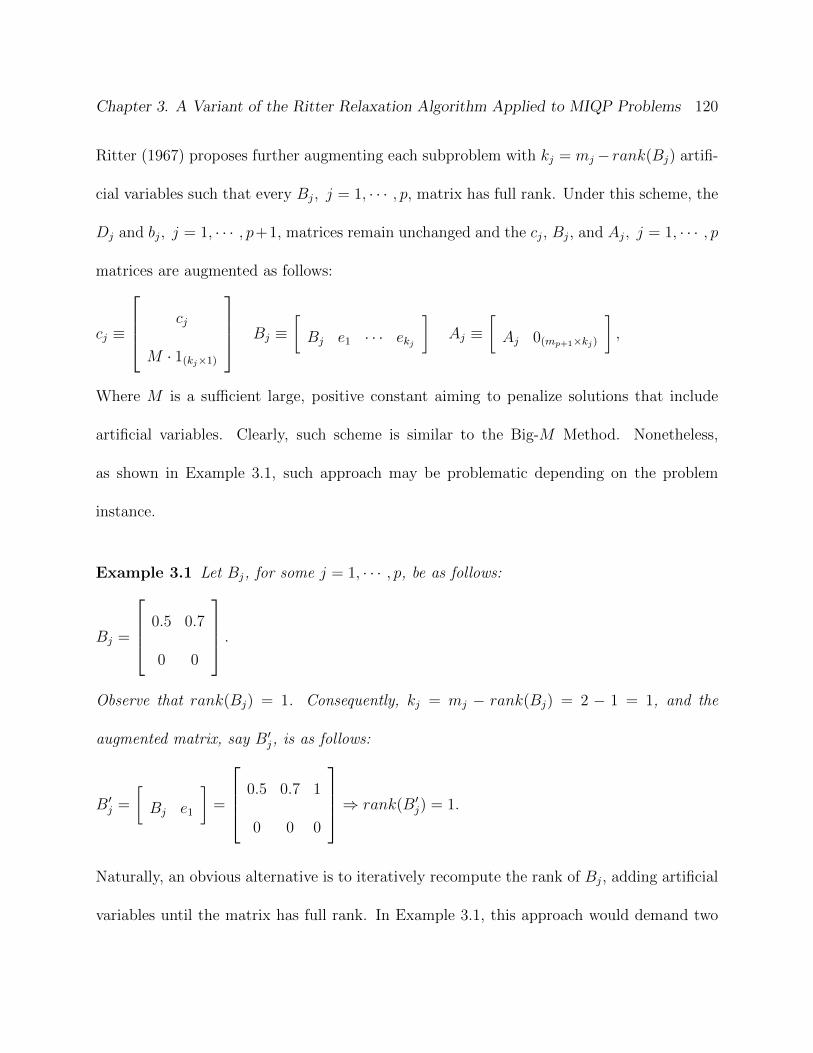
Chapter 3. A Variant of the Ritter Relaxation Algorithm Applied to MIQP Problems 120
Ritter (1967) proposes further augmenting each subproblem with kj = mj− rank(Bj) artifi-
cial variables such that every Bj, j = 1, · · · , p, matrix has full rank. Under this scheme, the
Dj and bj, j = 1, · · · , p+1, matrices remain unchanged and the cj, Bj, and Aj, j = 1, · · · , p
matrices are augmented as follows:
cj ≡
cj
M · 1(kj×1)
Bj ≡
[Bj e1 · · · ekj
]Aj ≡
[Aj 0(mp+1×kj)
],
Where M is a sufficient large, positive constant aiming to penalize solutions that include
artificial variables. Clearly, such scheme is similar to the Big-M Method. Nonetheless,
as shown in Example 3.1, such approach may be problematic depending on the problem
instance.
Example 3.1 Let Bj, for some j = 1, · · · , p, be as follows:
Bj =
0.5 0.7
0 0
.
Observe that rank(Bj) = 1. Consequently, kj = mj − rank(Bj) = 2 − 1 = 1, and the
augmented matrix, say B′j, is as follows:
B′j =
[Bj e1
]=
0.5 0.7 1
0 0 0
⇒ rank(B′j) = 1.
Naturally, an obvious alternative is to iteratively recompute the rank of Bj, adding artificial
variables until the matrix has full rank. In Example 3.1, this approach would demand two
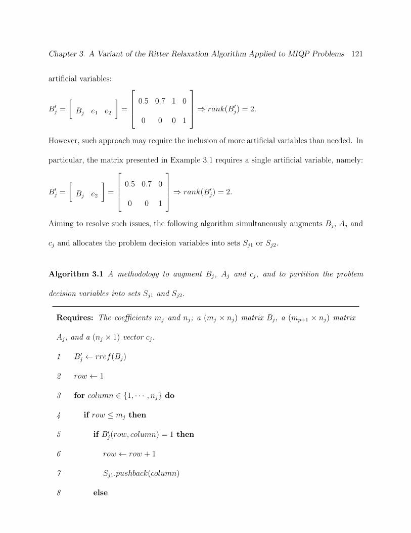
Chapter 3. A Variant of the Ritter Relaxation Algorithm Applied to MIQP Problems 121
artificial variables:
B′j =
[Bj e1 e2
]=
0.5 0.7 1 0
0 0 0 1
⇒ rank(B′j) = 2.
However, such approach may require the inclusion of more artificial variables than needed. In
particular, the matrix presented in Example 3.1 requires a single artificial variable, namely:
B′j =
[Bj e2
]=
0.5 0.7 0
0 0 1
⇒ rank(B′j) = 2.
Aiming to resolve such issues, the following algorithm simultaneously augments Bj, Aj and
cj and allocates the problem decision variables into sets Sj1 or Sj2.
Algorithm 3.1 A methodology to augment Bj, Aj and cj, and to partition the problem
decision variables into sets Sj1 and Sj2.
Requires: The coefficients mj and nj; a (mj × nj) matrix Bj, a (mp+1 × nj) matrix
Aj, and a (nj × 1) vector cj.
1 B′j ← rref(Bj)
2 row ← 1
3 for column ∈ {1, · · · , nj} do
4 if row ≤ mj then
5 if B′j(row, column) = 1 then
6 row ← row + 1
7 Sj1.pushback(column)
8 else
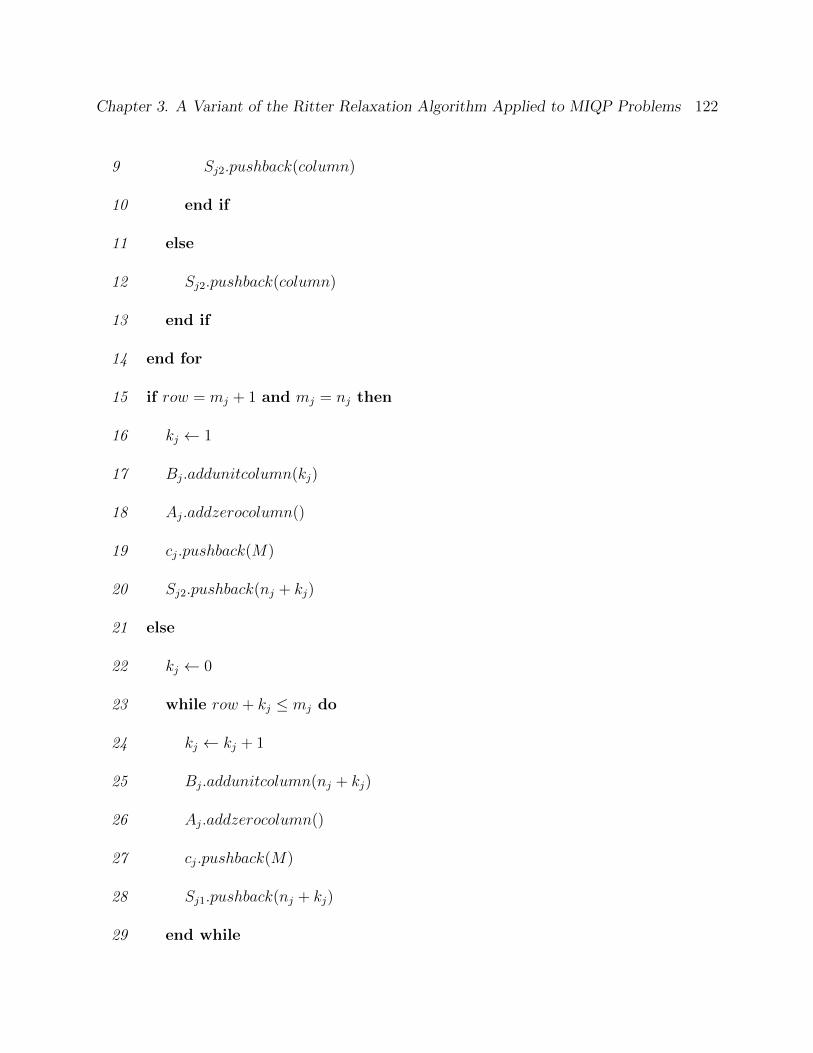
Chapter 3. A Variant of the Ritter Relaxation Algorithm Applied to MIQP Problems 122
9 Sj2.pushback(column)
10 end if
11 else
12 Sj2.pushback(column)
13 end if
14 end for
15 if row = mj + 1 and mj = nj then
16 kj ← 1
17 Bj.addunitcolumn(kj)
18 Aj.addzerocolumn()
19 cj.pushback(M)
20 Sj2.pushback(nj + kj)
21 else
22 kj ← 0
23 while row + kj ≤ mj do
24 kj ← kj + 1
25 Bj.addunitcolumn(nj + kj)
26 Aj.addzerocolumn()
27 cj.pushback(M)
28 Sj1.pushback(nj + kj)
29 end while
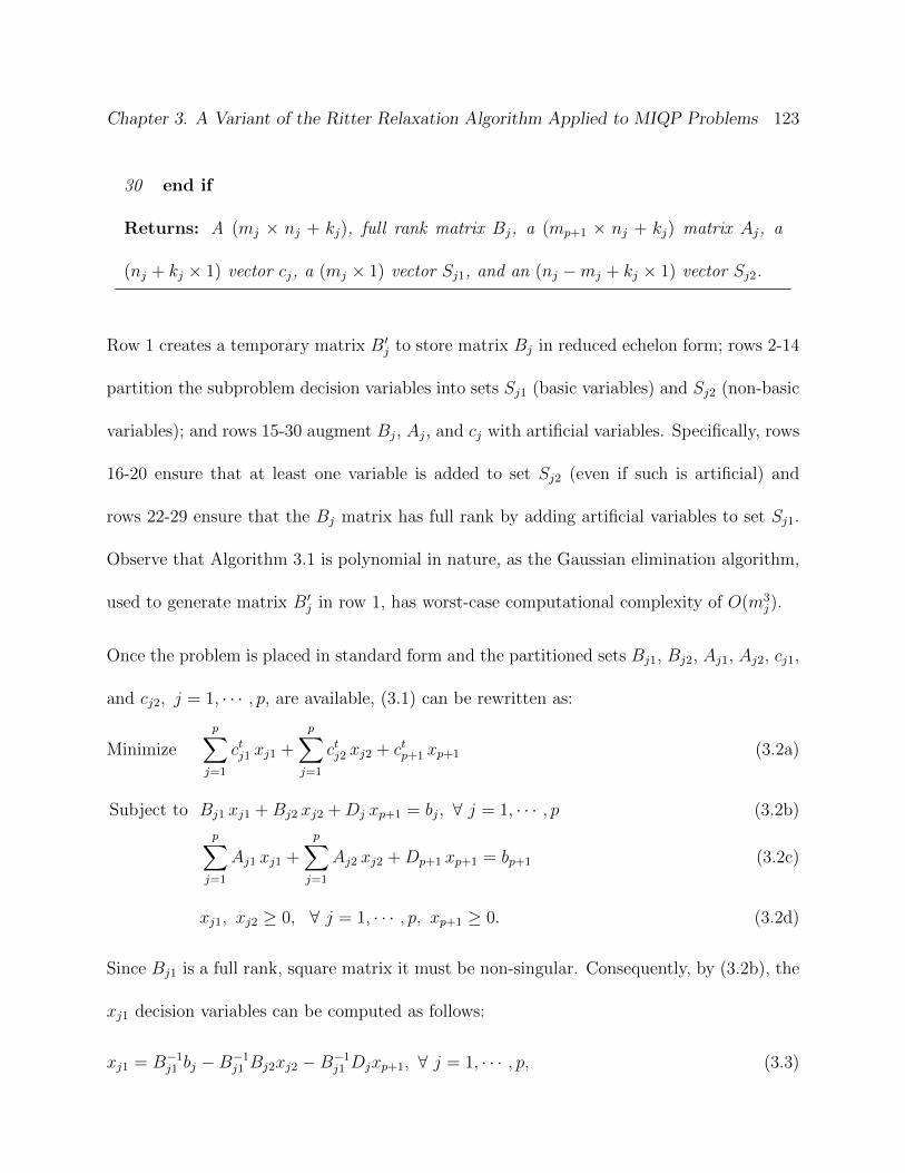
Chapter 3. A Variant of the Ritter Relaxation Algorithm Applied to MIQP Problems 123
30 end if
Returns: A (mj × nj + kj), full rank matrix Bj, a (mp+1 × nj + kj) matrix Aj, a
(nj + kj × 1) vector cj, a (mj × 1) vector Sj1, and an (nj −mj + kj × 1) vector Sj2.
Row 1 creates a temporary matrix B′j to store matrix Bj in reduced echelon form; rows 2-14
partition the subproblem decision variables into sets Sj1 (basic variables) and Sj2 (non-basic
variables); and rows 15-30 augment Bj, Aj, and cj with artificial variables. Specifically, rows
16-20 ensure that at least one variable is added to set Sj2 (even if such is artificial) and
rows 22-29 ensure that the Bj matrix has full rank by adding artificial variables to set Sj1.
Observe that Algorithm 3.1 is polynomial in nature, as the Gaussian elimination algorithm,
used to generate matrix B′j in row 1, has worst-case computational complexity of O(m3j).
Once the problem is placed in standard form and the partitioned sets Bj1, Bj2, Aj1, Aj2, cj1,
and cj2, j = 1, · · · , p, are available, (3.1) can be rewritten as:
Minimize
p∑
j=1
ctj1 xj1 +
p∑
j=1
ctj2 xj2 + ctp+1 xp+1 (3.2a)
Subject to Bj1 xj1 +Bj2 xj2 +Dj xp+1 = bj, ∀ j = 1, · · · , p (3.2b)
p∑
j=1
Aj1 xj1 +
p∑
j=1
Aj2 xj2 +Dp+1 xp+1 = bp+1 (3.2c)
xj1, xj2 ≥ 0, ∀ j = 1, · · · , p, xp+1 ≥ 0. (3.2d)
Since Bj1 is a full rank, square matrix it must be non-singular. Consequently, by (3.2b), the
xj1 decision variables can be computed as follows:
xj1 = B−1j1 bj −B−1
j1 Bj2xj2 −B−1j1 Djxp+1, ∀ j = 1, · · · , p, (3.3)

Chapter 3. A Variant of the Ritter Relaxation Algorithm Applied to MIQP Problems 124
And (3.2), after some rearrangement of the terms, becomes:
Minimize
p∑
j=1
(ctj2 − ctj1B−1
j1 Bj2
)xj2 +
(ctp+1 −
p∑
j=1
ctj1B−1j1 Dj
)xp+1 +
p∑
j=1
ctj1B−1j1 bj (3.4a)
Subject to
p∑
j=1
(Aj2 − Aj1B−1
j1 Bj2
)xj2 +
(Dp+1 −
p∑
j=1
Aj1B−1j1 Dj
)xp+1
= bp+1 −p∑
j=1
Aj1B−1j1 bj (3.4b)
xj2 ≥ 0, ∀ j = 1, · · · , p, xp+1 ≥ 0. (3.4c)
Observe that (3.4) does not encompass the non-negativity restriction on the xj1, j = 1, · · · , p,
decision variables. Now, for simplicity, let the following parameter substitutions be made:
dtj = ctj2 − ctj1B−1j1 Bj2, ∀ j = 1, · · · , p (3.5a)
dtp+1 = ctp+1 −p∑
j=1
ctj1B−1j1 Dj (3.5b)
α =
p∑
j=1
ctj1B−1j1 bj (3.5c)
Fj = Aj2 − Aj1B−1j1 Bj2, ∀ j = 1, · · · , p (3.5d)
Fp+1 = Dp+1 −p∑
j=1
Aj1B−1j1 Dj (3.5e)
f = bp+1 −p∑
j=1
Aj1B−1j1 bj. (3.5f)
Consequently, (3.4) can be written as the Reduced Problem:
Minimize
p∑
j=1
dtj xj2 + dtp+1 xp+1 + α (3.6a)
Subject to
p∑
j=1
Fj xj2 + Fp+1 xp+1 = f (3.6b)
Chapter 3. A Variant of the Ritter Relaxation Algorithm Applied to MIQP Problems 125
xj2 ≥ 0, ∀ j = 1, · · · , p, xp+1 ≥ 0. (3.6c)
Since xj2 and xp+1 can be used to compute the corresponding value for the xj1 decision
variables via (3.3), it follows that the feasible region of the Reduced Problem encompasses
the feasible region of the original problem. This, property, in fact, is formally proven in the
next Section. Observe that the Reduced Problem is a relaxation of the original problem, as
the non-negativity restriction on the xj1, j = 1, · · · , p, decision variables are not enforced.
In addition, some instances of (3.6) may be unbounded even if the optimal solution for
(3.1) is finite. In order to avoid the ensuing computational problems, Ritter (1967) suggests
including the constraint∑p
j=1 1(1×|Sj2|)xj2 + 1(1×np+1)xp+1 ≤ M in the Reduced Problem.
Note that, by letting xij2 and xip+1 denote, respectively, the ith element of xj2 and xp+1, such
constraint can be rewritten as:
p∑
j=1
|Sj2|∑
i=1
xij2 +
np+1∑
i=1
xip+1 ≤M. (3.7)
After the Reduced Problem, along with (3.7), is generated and solved, its optimum solution,
{x∗j2, j = 1, · · · , p, x∗p+1}, is used to find the corresponding solution for the relaxed variables,
{x∗j1, j = 1, · · · , p}, through Equation (3.3). If xij1 ≥ 0, ∀ j = 1, · · · , p, i = 1, · · · , |Sj1|, that
is, if the current solution is feasible to the original problem, then the algorithm terminates
with optimal solution {x∗j1, x∗j2, j = 1, · · · , p, x∗p+1} stripped of any previously added non-
basic artificial variables. As in the Big-M method, if the optimum solution has positive
(basic) artificial variables, then the original problem is infeasible. Conversely, if there exists
a subproblem j with a negative decision variable, say xij1, then such can either be swapped

Chapter 3. A Variant of the Ritter Relaxation Algorithm Applied to MIQP Problems 126
with a positive decision variable in set Sj2, say xkj2, or its non-negativity restriction can be
explicitly enforced in the Reduced Problem through an additional constraint. Consider the
following cases:
Case 1: Swap Elements. Suppose that, after the Reduced Problem is generated and solved
and the corresponding solution for the xj1, j = 1, · · · , p, decision variables are com-
puted, the ith element of set Sj1 is negative and the kth element of set Sj2 is positive,
that is, suppose that xij1 < 0 and xkj2 > 0 for some subproblem j = 1, · · · , p. Then,
the relaxed variable xij1 may be assigned to set Sj2 and the non-relaxed variable xkj2 as-
signed to set Sj1 as long as the ith row, kth column element of matrix B−1j1 Bj2 6= 0. Such
restriction ensures that the new Bj1 matrix, generated after these decision variables
are swapped, remains non-singular.
Case 2: Explicitly enforce the non-negativity restriction of xij1. If no positive elements on Sj2
exist or if the ith row, kth column element of matrix B−1j1 Bj2 = 0, ∀ i ∈ {Sj1 : xij1 < 0}
and k ∈ {Sj2 : xkj2 > 0}, then the non-negativity restriction on xij1 must be explicitly
enforced in the Reduced Problem through an additional constraint, namely:
xij1 ≥ 0⇔ {B−1j1 bj}i − {B−1
j1 Bj2}i xj2 − {B−1j1 Dj}i xp+1 ≥ 0
⇔ {B−1j1 Bj2}i xj2 + {B−1
j1 Dj}i xp+1 ≤ {B−1j1 bj}i, (3.8)
Where the notation {B−1j1 Bj2}i, for instance, indicates the ith row of the matrix B−1
j1 Bj2.
While any negative relaxed decision variable can have its non-negativity restriction
enforced via (3.8), it is reasonable to enforce only the restriction of the most negative

Chapter 3. A Variant of the Ritter Relaxation Algorithm Applied to MIQP Problems 127
element in set Sj1, as to maintain the size of the Reduced Problem small, and, thus,
computationally tractable.
Observe that only one of these cases is applicable to each subproblem, as any changes in
the problem structure results in a new optimum solution {x∗j1, x∗j2, j = 1, · · · , p, x∗p+1},
and, thus, in a new set of negative {x∗j1, j = 1, · · · , p}, elements. Moreover, from Case 2,
it is clear that the original problem can be solved in a single iteration by having all the
relaxed non-negativity restrictions enforced through (3.8). Nonetheless, since such a large
number of constraints would offset the benefits of the relaxation, improved solution times
are attained when only the biding restrictions are maintained. In fact, subsequent iterations
of the algorithm evaluate whether previously added constraints of this form can be removed.
Suppose that, on a previous iteration of the algorithm, the non-negativity restriction of the
ith relaxed decision variable of the jth subproblem was enforced as in Case 2. Consider the
following cases:
Case 3: Constraint (3.8) is non-binding. If, for a current optimum solution to the Reduced
Problem, {x∗j2, j = 1, · · · , p, x∗p+1}, (3.8) is non-binding, that is, if {B−1j1 Bj2}ix∗j2 +
{B−1j1 Dj}ix∗p+1 < {B−1
j1 bj}i ⇔ xij1 > 0, then the constraint can be removed without
affecting the current solution {x∗j1, x∗j2, j = 1, · · · , p, x∗p+1}.
Case 4: Constraint (3.8) is biding, but the respective xij1 decision variable can be swapped
with a positive element in xj2. If, for a current optimum solution to the Reduced
Problem, {x∗j2, j = 1, · · · , p, x∗p+1}, (3.8) is binding, that is, if {B−1j1 Bj2}ix∗j2 +
Chapter 3. A Variant of the Ritter Relaxation Algorithm Applied to MIQP Problems 128
{B−1j1 Dj}ix∗p+1 = {B−1
j1 bj}i ⇔ xij1 = 0, then the constraint can be removed if there
exists a strictly positive element k in set Sj2, such that the ith row, kth column element
of matrix B−1j1 Bj2 6= 0. Since the swap operation only reorganizes the decision vari-
ables into sets Sj1 and Sj2, removing (3.8) from the Reduced Problem does not alter
its current solution.
In summary, the original Ritter (1967) Relaxation Algorithm proceeds as follows:
1. For each subproblem j = 1, · · · , p, augment the Bj, Aj, and cj matrices with artificial
variables in order to ensure that Bj has full rank, and, at least, mj + 1 columns;
2. For each subproblem j = 1, · · · , p, partition the columns of Bj and Aj and the rows
of cj into sets Bj1 and Bj2, Aj1 and Aj2, and cj1 and cj2 such that Bj1 is non-singular.
Note that the previous step and the decision variable partitioning into sets Sj1 and Sj2
may be accomplished simultaneously, for instance, through Algorithm 3.1;
3. Given the partitions Bj1 and Bj2, Aj1 and Aj2, and cj1 and cj2, j = 1, · · · , p, compute
parameters (3.5) and use such parameters, along with Constraint (3.7), to generate
the Reduced Problem (3.6). Solve the Reduced Problem. If no feasible solution to the
Reduced Problem exists, then the original problem is infeasible. Terminate;
4. Given the optimum solution to the Reduced Problem, {x∗j2, j = 1, · · · , p, x∗p+1},
use (3.3) to compute the corresponding solution to the relaxed variables, {x∗j1, j =
1, · · · , p}. If all relaxed variables are non-negative, terminate:
Chapter 3. A Variant of the Ritter Relaxation Algorithm Applied to MIQP Problems 129
• If any of the artificial variables added in Step 1 are positive (basic), then the
original problem is either infeasible or unbounded;
• If all artificial variables equal zero, but Constraint (3.7) is binding, then the
original problem is unbounded; otherwise
• The solution attained is optimal to the original problem;
5. If any Constraint of the form (3.8) have been added on previous iterations, then evalu-
ate whether those may be removed. If the constraint is non-binding, then remove it as
in Case 3; otherwise, search set Sj2 for a positive decision variable xkj2, such that the
ith row, kth column element of matrix B−1j1 Bj2 6= 0. If such variable exists, then swap
them as in Case 4 and remove (3.8); otherwise maintain the constraint unchanged;
6. For each subproblem j = 1, · · · , p, if there exists a negative element in set Sj1 and
a positive element in set Sj2 (i.e., if xij1 < 0 and xkj2 > 0), such that the ith row,
kth column element of matrix B−1j1 Bj2 6= 0, then swap these variables as in Case 1;
otherwise, explicitly enforce the non-negativity restriction of the most negative variable
in Sj1 as in Case 2. Return to Step 3.
Next, a modification to the Ritter (1967) Relaxation Algorithm able to solve bordered-
structure problems with linear, integer, or mixed-integer subproblems and with linear or
quadratic objective functions is presented.

Chapter 3. A Variant of the Ritter Relaxation Algorithm Applied to MIQP Problems 130
3.2.2 Modified Algorithm
Recall that the Ritter (1967) Relaxation Algorithm enforces violated non-negativity restric-
tions either by swapping elements between the relaxed and non-relaxed sets (as in Case 1)
or by adding constraints of the form (3.8) into the Reduced Problem (as in Case 2). In fact,
the algorithm favors the swap operation, as constraints of the form (3.8) are only added to
the Reduced Problem if all non-relaxed variables equal zero or if strictly positive elements in
Sj2 exist, but swapping them with negative elements in Sj1 results in singular Bj1 matrices.
Moreover, previously added constraints of the form (3.8) are removed whenever they are
non-binding (as in Case 3) or the non-negativity restriction of their referenced decision vari-
ables can be enforced by swapping (as in Case 4). By favoring the swap operation, the Ritter
(1967) Relaxation Algorithm is able to maintain the size of the Reduced Problem small, and,
thus, relatively quick to solve. Nonetheless, the increased number of matrix inversions and
multiplications involved in the swap operation not only offset the reduced computation time
attained by the relaxation, but may also lead to considerable machine-precision issues. In
this Section, a variation of the Ritter (1967) Relaxation Algorithm, which relies solely on
the addition and removal of constraints from the Reduced Problem, is presented.
First, however, some important modifications to the problem definition are warranted. Recall
that the Ritter (1967) Relaxation Algorithm requires the problem to be placed in standard
form. While such operation is often performed during the initialization of many commonly
used solution algorithms, such as Simplex and Revised Simplex, the inclusion of such large
number of slack variables increases the complexity of the Reduced Problem, thus possibly

Chapter 3. A Variant of the Ritter Relaxation Algorithm Applied to MIQP Problems 131
slowing its solution time (e.g., if alternative solution methodologies, such as Network Simplex
and Interior Point Methods, are used to solve the Reduced Problem). Naturally, such trans-
formation is essential for the algorithm, as placing the original problem in standard form
allows an algebraic solution to xj1, j = 1, · · · , p, decision variables to be derived, which, in
turn, allows such decision variables to be eliminated from the Reduced Problem by substi-
tution. Nonetheless, other than (3.7), all the structural constraints of the Reduced Problem
generated on the first iteration of the Ritter (1967) Relaxation Algorithm follow from the
complicating constraints in the original problem, and, as such, do not need to be placed
in standard form. By avoiding the inclusion of the slack variables corresponding to these
constraints, depending on the solution methodology used to solve the Reduced Problem, it
is possible to improve the performance of the Ritter (1967) Relaxation Algorithm.
In addition, recall that the original algorithm was developed for continuous (convex) prob-
lems, whereas many important optimization problems contain integer decision variables.
Since the swap operation enforces violated non-negativity restrictions of the decision vari-
ables in the relaxed set by placing them in the non-relaxed set (where their non-negativity
restriction remains enforced), it stands to reason that such operation could also allow in-
teger restrictions to be similarly enforced. Unfortunately, while such is indeed the case
for the element entering set Sj2, it is not the case, in general, for the element leaving Sj2
and entering Sj1, for, after the Reduced Problem is reoptimized, any new (integer) solution
{x∗j2, j = 1, · · · , p, x∗p+1} results in a new (possibly non-integer) solution {x∗j1, j = 1, · · · , p}.
As a result, the swap operation not only reduces the performance of the algorithm and leads
Chapter 3. A Variant of the Ritter Relaxation Algorithm Applied to MIQP Problems 132
to considerable machine-precision issues, but it also leads to cycling and possibly stalling
when attempting to solve problems with integer or mixed-integer subproblems. Nonetheless,
if only constraints of the form (3.8) are added to the Reduced Problem, then the integer
restriction of the decision variables in the relaxed set can be enforced in a scheme similar to
the branch and bound algorithm. Consider the following generic, mixed-integer problem:
Minimize
p+1∑
j=1
ctj xj (3.9a)
Subject to Bj xj + Imjyj +Dj xp+1 = bj, ∀ j = 1, · · · , p (3.9b)
p∑
j=1
Aeqj xj +Deq xp+1 = beq (3.9c)
p∑
j=1
Aineqj xj +Dineq xp+1 ≤ bineq (3.9d)
xj ∈ (R+ × Z+), ∀ j = 1, · · · , p+ 1 (3.9e)
yj ∈ R+, ∀ j = 1, · · · , p, (3.9f)
Where yj are the slack variables corresponding to Constraint (3.1b); Aeqj, Aineqj, Deq, and
Dineq are, respectively, (meq × nj), (mineq × nj), (meq × np+1), and (mineq × np+1) matrices
of constraint coefficients; and beq and bineq are column vectors of meq and mineq right hand
side coefficients, respectively. The notation (R+ × Z+) indicates the non-negative, mixed-
integer nature of the problem. Although (3.9) allows for the possibility of mixed-integer
subproblems and parses the complicating constraints of the original problem into equalities
and inequalities, the inheriting bordered-structure of (3.1) remains unchanged.
In general, the Modified Ritter (1967) Relaxation Algorithm relies on the same steps of the

Chapter 3. A Variant of the Ritter Relaxation Algorithm Applied to MIQP Problems 133
original algorithm save for the swap operation. Consequently, the non-negativity restriction
of any negative variable in the relaxed set is enforced solely by constraints of the form (3.8).
However, contrary to the original algorithm where previously added constraints of this form
may be removed if they are non-binding, here, such constraints are only removed provided
they are redundant. Moreover, since the problem decision variables are no longer swapped
between the relaxed and non-relaxed sets, the corresponding Bj1, Bj2, Aj1, Aj2, cj1, and
cj2, j = 1, · · · , p, partitions remain unchanged throughout the execution of the algorithm.
Hence, the following constants can be computed a priori and reused as needed:
Bj = B−1j1 Bj2, ∀ j = 1, · · · , p (3.10a)
Dj = B−1j1 Dj, ∀ j = 1, · · · , p (3.10b)
bj = B−1j1 bj, ∀ j = 1, · · · , p. (3.10c)
Consequently, (3.3) simplifies to:
xj1 = B−1j1 bj −B−1
j1 Bj2 xj2 −B−1j1 Dj xp+1, ∀ j = 1, · · · , p
= bj −Bj xj2 −Dj xp+1, ∀ j = 1, · · · , p, (3.11)
Equation (3.8) simplifies to:
xij1 ≥ 0⇔ {B−1j1 Bj2}i xj2 + {B−1
j1 Dj}i xp+1 ≤ {B−1j1 bj}i
⇔ {Bj}i xj2 + {Dj}i xp+1 ≤ {bj}i, (3.12)
And (3.5), after allowing for the possibility of both equality and inequality complicating
constraints, change to:
dtj = ctj2 − ctj1Bj, ∀ j = 1, · · · , p (3.13a)
Chapter 3. A Variant of the Ritter Relaxation Algorithm Applied to MIQP Problems 134
dtp+1 = ctp+1 −p∑
j=1
ctj1Dj (3.13b)
α =
p∑
j=1
ctj1 bj (3.13c)
Fj = Aeqj2 − Aeqj1Bj, ∀ j = 1, · · · , p (3.13d)
Fp+1 = Deq −p∑
j=1
Aeqj1Dj (3.13e)
f = beq −p∑
j=1
Aeqj1 bj (3.13f)
Gj = Aineqj2 − Aineqj1Bj, ∀ j = 1, · · · , p (3.13g)
Gp+1 = Dineq −p∑
j=1
Aineqj1Dj (3.13h)
g = bineq −p∑
j=1
Aineqj1 bj. (3.13i)
After the appropriate parameter substitutions and the inclusion of Constraint (3.7), the
resulting Reduced Problem is as follows:
Minimize
p∑
j=1
dtj xj2 + dtp+1 xp+1 + α (3.14a)
Subject to
p∑
j=1
Fj xj2 + Fp+1 xp+1 = f (3.14b)
p∑
j=1
Gj xj2 +Gp+1 xp+1 ≤ g (3.14c)
p∑
j=1
|Sj2|∑
i=1
xij2 +
np+1∑
i=1
xip+1 ≤M (3.14d)
xj2 ∈ (R+ × Z+), ∀ j = 1, · · · , p, xp+1 ∈ (R+ × Z+). (3.14e)
As aforementioned, constraints of the form (3.8), or, now (3.12), not only can be used to
Chapter 3. A Variant of the Ritter Relaxation Algorithm Applied to MIQP Problems 135
enforce non-negativity restrictions, but also the integer restriction of any decision variable in
the relaxed set. For instance, suppose that, on some iteration of the Modified Ritter (1967)
Relaxation Algorithm, the ith relaxed element of the jth subproblem attains a fractional (but
positive) value a, then, following a scheme similar to the branch and bound algorithm, two
new subproblems are generated and solved, namely:
Branch I of the Reduced Problem:
xij1 ≤ bac ⇔ {bj}i − {Bj}i xj2 − {Dj}i xp+1 ≤ bac
⇔ −{Bj}i xj2 − {Dj}i xp+1 ≤ bac − {bj}i. (3.15a)
Branch II of the Reduced Problem:
xij1 ≥ dae ⇔ {bj}i − {Bj}i xj2 − {Dj}i xp+1 ≥ dae
⇔ {Bj}i xj2 + {Dj}i xp+1 ≤ −dae+ {bj}i. (3.15b)
Observe that no consideration has been given to the integer restriction, if any, of the deci-
sion variables in set Sj2, j = 1, · · · , p, as those are enforced within the Reduced Problem.
Consequently, the modified algorithm disaggregates the branch and bound tree that would
have been produced while solving the original problem into two separate trees: one enforced
by constraints of the form (3.15), and one enforced by whichever algorithm is used to solve
the Reduced Problem. As a result, the same concerns pertaining to the branch and bound
algorithm, such as branching strategy and choice of branching variable, also apply to the
modified algorithm. These, however, are beyond the scope of this research.
Moreover, recall that the modified algorithm only allows previously added constraints of

Chapter 3. A Variant of the Ritter Relaxation Algorithm Applied to MIQP Problems 136
the form (3.12), or, for that matter, (3.15), to be removed from the Reduced Problem
provided they are redundant (and not if they are simply non-binding). Such is an important
consideration, for it preserves the dichotomy of the branch and bound search, and thus
prevents cycling and, possibly, stalling.
Lastly, on any iteration of the modified algorithm, if one of the decision variables in the
relaxed set becomes negative, then an additional constraint of the form (3.12) is added to
the Reduced Problem and such is reoptimized before any other subsequent branches are
created. A similar approach is followed, for instance, to enforce the binary restriction of any
relaxed decision variables with values greater than one.
Next, a quadratic variation of the problem is presented. Consider problem (3.9), but, in-
stead of the linear Objective Function (3.9a), suppose that such problem has the quadratic
objective function {Minimize 0.5xtH x+ct x}, where H denotes its Hessian matrix (i.e., the
|x| × |x| matrix of its second-order partial derivatives). Following the notation used in (3.9),
let H be partitioned into (p+ 1)2 submatrices Hjk, j = 1, · · · , p+ 1, k = 1, · · · , p+ 1:
Minimize1
2
p+1∑
j=1
p+1∑
k=1
xtjHjkxk +
p+1∑
j=1
ctj xj. (3.16)
Now, following an scheme similar to the one used to derive (3.13), let the decision variables
of each subproblem j = 1, · · · , p, be partitioned into sets Sj1 and Sj2, and the corresponding
columns of Bj and Aj and the rows of cj be grouped into the disjoint sets Bj1 and Bj2,
Aj1 and Aj2, and cj1 and cj2. Moreover, let each of the Hjk, j = 1, · · · , p, k = 1, · · · , p,
submatrices be partitioned into four additional submatrices, Hjk11, Hjk12, Hjk21, and Hjk22;
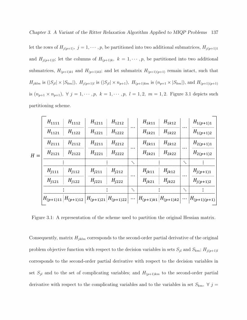
Chapter 3. A Variant of the Ritter Relaxation Algorithm Applied to MIQP Problems 137
let the rows of Hj(p+1), j = 1, · · · , p, be partitioned into two additional submatrices, Hj(p+1)1
and Hj(p+1)2; let the columns of H(p+1)k, k = 1, · · · , p, be partitioned into two additional
submatrices, H(p+1)k1 and H(p+1)k2; and let submatrix H(p+1)(p+1) remain intact, such that
Hjklm is (|Sjl| × |Skm|), Hj(p+1)l is (|Sjl| × np+1), H(p+1)km is (np+1 × |Skm|), and H(p+1)(p+1)
is (np+1 × np+1), ∀ j = 1, · · · , p, k = 1, · · · , p, l = 1, 2, m = 1, 2. Figure 3.1 depicts such
partitioning scheme.
Figure 3.1: A representation of the scheme used to partition the original Hessian matrix.
Consequently, matrix Hjklm corresponds to the second-order partial derivative of the original
problem objective function with respect to the decision variables in sets Sjl and Skm; Hj(p+1)l
corresponds to the second-order partial derivative with respect to the decision variables in
set Sjl and to the set of complicating variables; and H(p+1)km to the second-order partial
derivative with respect to the complicating variables and to the variables in set Skm, ∀ j =
Chapter 3. A Variant of the Ritter Relaxation Algorithm Applied to MIQP Problems 138
1, · · · , p, k = 1, · · · , p, l = 1, 2, m = 1, 2. As a result, (3.16) becomes:
Minimize1
2
p∑
j=1
p∑
k=1
[xtj1 xtj2
]Hjk11 Hjk12
Hjk21 Hjk22
xk1
xk2
+
+
p∑
j=1
[xtj1 xtj2
]Hj(p+1)1
Hj(p+1)2
xp+1 +
p∑
k=1
xtp+1
[H(p+1)k1 H(p+1)k2
]xk1
xk2
+
xtp+1H(p+1)(p+1)xp+1
)+
p∑
j=1
[ctj1 ctj2
]xj1
xj2
+ ctp+1xp+1.
Or, after fully expanding the matrix operations:
Minimize1
2
(p∑
j=1
p∑
k=1
(xtj1Hjk11xk1 + xtj2Hjk21xk1 + xtj1Hjk12xk2 + xtj2Hjk22xk2
)+
p∑
j=1
(xtj1Hj(p+1)1xp+1 + xtj2Hj(p+1)2xp+1
)+
p∑
k=1
(xtp+1H(p+1)k1xk1 + xtp+1H(p+1)k2xk2
)+
+ xtp+1H(p+1)(p+1)xp+1
)+
p∑
j=1
(ctj1xj1 + ctj2xj2
)+ ctp+1xp+1. (3.17)
Now, by (3.11), xj1 = bj − Bj xj2 − Dj xp+1, ∀ j = 1, · · · , p. Consequently, (3.17) can be
rewritten as:
Minimize1
2
(p∑
j=1
p∑
k=1
((bj −Bj xj2 −Dj xp+1
)tHjk11
(bk −Bk xk2 −Dk xp+1
)+
+xtj2Hjk21
(bk −Bk xk2 −Dk xp+1
)+(bj −Bj xj2 −Dj xp+1
)tHjk12xk2 + xtj2Hjk22xk2
)+
p∑
j=1
((bj −Bj xj2 −Dj xp+1
)tHj(p+1)1xp+1 + xtj2Hj(p+1)2xp+1
)+
+
p∑
k=1
(xtp+1H(p+1)k1
(bk −Bk xk2 −Dk xp+1
)+ xtp+1H(p+1)k2xk2
)+
+ xtp+1H(p+1)(p+1)xp+1
)+
p∑
j=1
(ctj1(bj −Bj xj2 −Dj xp+1
)+ ctj2xj2
)+ ctp+1xp+1,

Chapter 3. A Variant of the Ritter Relaxation Algorithm Applied to MIQP Problems 139
Or, after some index substitutions and some rearrangement of the terms, as:
Minimize1
2
p∑
j=1
p∑
k=1
xtj2
(Hjk22 −Bt
jHjk12 −Hjk21Bk +Bt
jHjk11Bk
)xk2+
1
2
p∑
j=1
xtj2
(Hj(p+1)2 −Bt
jHj(p+1)1 +
p∑
k=1
(Bt
jHjk11 −Hjk21
)Dk
)xp+1+
1
2
p∑
k=1
xtp+1
(H(p+1)k2 −H(p+1)k1Bk +
p∑
j=1
Dt
j
(Hjk11Bk −Hjk12
))xk2+
1
2xtp+1
(H(p+1)(p+1) −
p∑
j=1
(Dt
jHj(p+1)1 +H(p+1)j1Dj
)+
p∑
j=1
p∑
k=1
Dt
jHjk11Dk
)xp+1+
p∑
j=1
(ctj2 − ctj1Bj +
1
2
p∑
k=1
bt
k
(H tjk21 −H t
jk11Bj +Hkj12 −Hkj11Bj
))xj2+
(ctp+1 −
p∑
j=1
(ctj1Dj −
1
2bt
j
(Hj(p+1)1 +H t
(p+1)j1
)+
1
2
p∑
k=1
bt
j
(Hjk11 +H t
kj11
)Dk
))xp+1+
p∑
j=1
(ctj1bj +
1
2
p∑
k=1
bt
jHjk11bk
).
Now, let the following parameter substitutions be performed:
Ljk = Hjk22 −Bt
jHjk12 −Hjk21Bk +Bt
jHjk11Bk, ∀ j = 1, · · · , p, k = 1, · · · , p (3.18a)
Lj(p+1) = Hj(p+1)2 −Bt
jHj(p+1)1 +
p∑
k=1
(Bt
jHjk11 −Hjk21
)Dk, ∀ j = 1, · · · , p (3.18b)
L(p+1)k = H(p+1)k2 −H(p+1)k1Bk +
p∑
j=1
Dt
j
(Hjk11Bk −Hjk12
), ∀ k = 1, · · · , p (3.18c)
L(p+1)(p+1) = H(p+1)(p+1) −p∑
j=1
(Dt
jHj(p+1)1 +H(p+1)j1Dj
)+
p∑
j=1
p∑
k=1
Dt
jHjk11Dk (3.18d)
dtj = ctj2 − ctj1Bj +1
2
p∑
k=1
bt
k
(H tjk21 −H t
jk11Bj +Hkj12 −Hkj11Bj
), ∀ j = 1, · · · , p (3.18e)
dtp+1 = ctp+1 −p∑
j=1
(ctj1Dj −
1
2bt
j
(Hj(p+1)1 +H t
(p+1)j1
)+
1
2
p∑
k=1
bt
j
(Hjk11 +H t
kj11
)Dk
)
(3.18f)
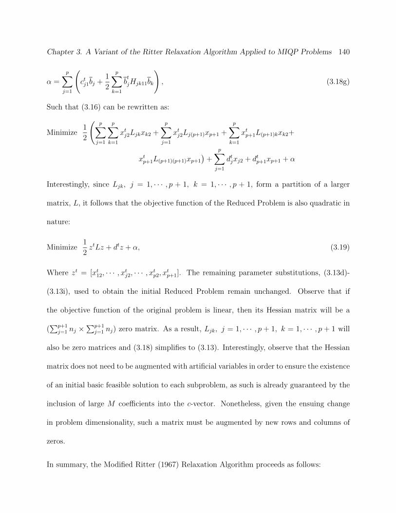
Chapter 3. A Variant of the Ritter Relaxation Algorithm Applied to MIQP Problems 140
α =
p∑
j=1
(ctj1bj +
1
2
p∑
k=1
bt
jHjk11bk
), (3.18g)
Such that (3.16) can be rewritten as:
Minimize1
2
(p∑
j=1
p∑
k=1
xtj2Ljkxk2 +
p∑
j=1
xtj2Lj(p+1)xp+1 +
p∑
k=1
xtp+1L(p+1)kxk2+
xtp+1L(p+1)(p+1)xp+1
)+
p∑
j=1
dtjxj2 + dtp+1xp+1 + α
Interestingly, since Ljk, j = 1, · · · , p + 1, k = 1, · · · , p + 1, form a partition of a larger
matrix, L, it follows that the objective function of the Reduced Problem is also quadratic in
nature:
Minimize1
2ztLz + dtz + α, (3.19)
Where zt = [xt12, · · · , xtj2, · · · , xtp2, xtp+1]. The remaining parameter substitutions, (3.13d)-
(3.13i), used to obtain the initial Reduced Problem remain unchanged. Observe that if
the objective function of the original problem is linear, then its Hessian matrix will be a
(∑p+1
j=1 nj ×∑p+1
j=1 nj) zero matrix. As a result, Ljk, j = 1, · · · , p + 1, k = 1, · · · , p + 1 will
also be zero matrices and (3.18) simplifies to (3.13). Interestingly, observe that the Hessian
matrix does not need to be augmented with artificial variables in order to ensure the existence
of an initial basic feasible solution to each subproblem, as such is already guaranteed by the
inclusion of large M coefficients into the c-vector. Nonetheless, given the ensuing change
in problem dimensionality, such a matrix must be augmented by new rows and columns of
zeros.
In summary, the Modified Ritter (1967) Relaxation Algorithm proceeds as follows:
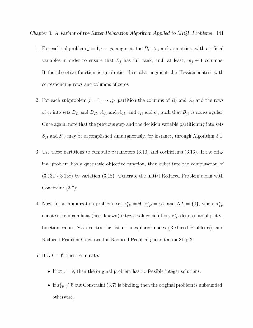
Chapter 3. A Variant of the Ritter Relaxation Algorithm Applied to MIQP Problems 141
1. For each subproblem j = 1, · · · , p, augment the Bj, Aj, and cj matrices with artificial
variables in order to ensure that Bj has full rank, and, at least, mj + 1 columns.
If the objective function is quadratic, then also augment the Hessian matrix with
corresponding rows and columns of zeros;
2. For each subproblem j = 1, · · · , p, partition the columns of Bj and Aj and the rows
of cj into sets Bj1 and Bj2, Aj1 and Aj2, and cj1 and cj2 such that Bj1 is non-singular.
Once again, note that the previous step and the decision variable partitioning into sets
Sj1 and Sj2 may be accomplished simultaneously, for instance, through Algorithm 3.1;
3. Use these partitions to compute parameters (3.10) and coefficients (3.13). If the orig-
inal problem has a quadratic objective function, then substitute the computation of
(3.13a)-(3.13c) by variation (3.18). Generate the initial Reduced Problem along with
Constraint (3.7);
4. Now, for a minimization problem, set x∗IP = ∅, z∗IP = ∞, and NL = {0}, where x∗IP
denotes the incumbent (best known) integer-valued solution, z∗IP denotes its objective
function value, NL denotes the list of unexplored nodes (Reduced Problems), and
Reduced Problem 0 denotes the Reduced Problem generated on Step 3;
5. If NL = ∅, then terminate:
• If x∗IP = ∅, then the original problem has no feasible integer solutions;
• If x∗IP 6= ∅ but Constraint (3.7) is binding, then the original problem is unbounded;
otherwise,
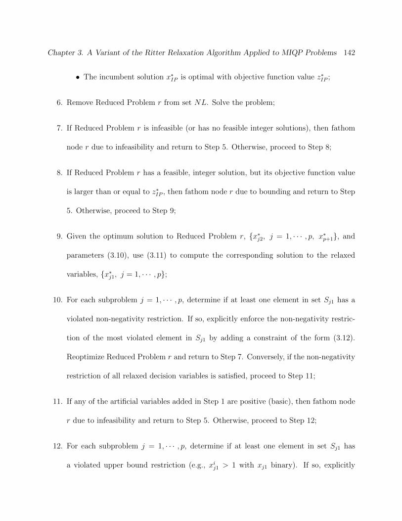
Chapter 3. A Variant of the Ritter Relaxation Algorithm Applied to MIQP Problems 142
• The incumbent solution x∗IP is optimal with objective function value z∗IP ;
6. Remove Reduced Problem r from set NL. Solve the problem;
7. If Reduced Problem r is infeasible (or has no feasible integer solutions), then fathom
node r due to infeasibility and return to Step 5. Otherwise, proceed to Step 8;
8. If Reduced Problem r has a feasible, integer solution, but its objective function value
is larger than or equal to z∗IP , then fathom node r due to bounding and return to Step
5. Otherwise, proceed to Step 9;
9. Given the optimum solution to Reduced Problem r, {x∗j2, j = 1, · · · , p, x∗p+1}, and
parameters (3.10), use (3.11) to compute the corresponding solution to the relaxed
variables, {x∗j1, j = 1, · · · , p};
10. For each subproblem j = 1, · · · , p, determine if at least one element in set Sj1 has a
violated non-negativity restriction. If so, explicitly enforce the non-negativity restric-
tion of the most violated element in Sj1 by adding a constraint of the form (3.12).
Reoptimize Reduced Problem r and return to Step 7. Conversely, if the non-negativity
restriction of all relaxed decision variables is satisfied, proceed to Step 11;
11. If any of the artificial variables added in Step 1 are positive (basic), then fathom node
r due to infeasibility and return to Step 5. Otherwise, proceed to Step 12;
12. For each subproblem j = 1, · · · , p, determine if at least one element in set Sj1 has
a violated upper bound restriction (e.g., xij1 > 1 with xj1 binary). If so, explicitly
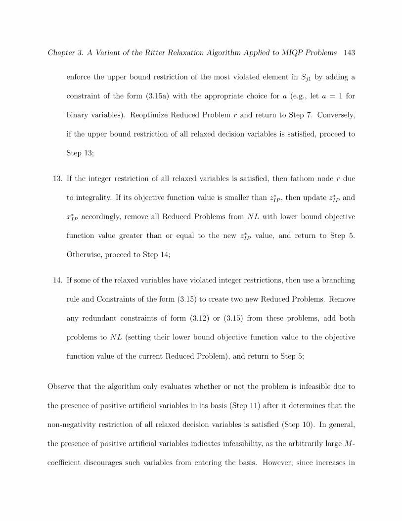
Chapter 3. A Variant of the Ritter Relaxation Algorithm Applied to MIQP Problems 143
enforce the upper bound restriction of the most violated element in Sj1 by adding a
constraint of the form (3.15a) with the appropriate choice for a (e.g., let a = 1 for
binary variables). Reoptimize Reduced Problem r and return to Step 7. Conversely,
if the upper bound restriction of all relaxed decision variables is satisfied, proceed to
Step 13;
13. If the integer restriction of all relaxed variables is satisfied, then fathom node r due
to integrality. If its objective function value is smaller than z∗IP , then update z∗IP and
x∗IP accordingly, remove all Reduced Problems from NL with lower bound objective
function value greater than or equal to the new z∗IP value, and return to Step 5.
Otherwise, proceed to Step 14;
14. If some of the relaxed variables have violated integer restrictions, then use a branching
rule and Constraints of the form (3.15) to create two new Reduced Problems. Remove
any redundant constraints of form (3.12) or (3.15) from these problems, add both
problems to NL (setting their lower bound objective function value to the objective
function value of the current Reduced Problem), and return to Step 5;
Observe that the algorithm only evaluates whether or not the problem is infeasible due to
the presence of positive artificial variables in its basis (Step 11) after it determines that the
non-negativity restriction of all relaxed decision variables is satisfied (Step 10). In general,
the presence of positive artificial variables indicates infeasibility, as the arbitrarily large M -
coefficient discourages such variables from entering the basis. However, since increases in
Chapter 3. A Variant of the Ritter Relaxation Algorithm Applied to MIQP Problems 144
the objective function value resulting from such variables may be offset by the presence of
negative basic variables (artificial or not), it follows that these, by themselves, do not imply
infeasibility. In fact, since the relaxed set may also contain artificial variables, since their
non-negativity restriction is relaxed, since the transformations used to attain the Reduced
Problem do not alter the objective function of the original problem (other than reducing its
dimensionality), and since M is arbitrary large, it follows that the Reduced Problem will (for
a minimization problem) favor large negative values for such artificial variables. Therefore,
artificial variables must be treated as regular decision variables until the non-negativity
restriction of all the elements in the relaxed set are satisfied. Once it is determined that such
problems are indeed infeasible, the node is fathomed, as any child nodes resulting from the
inclusion of additional constraints of the form (3.15) will also be infeasible. Note that such
fathoming criterion follows directly from the Big-M method, for feasibility is not prevented
by basic artificial variables that equal zero: it is possible for the Reduced Problem to have an
alternate basis representation in which such variables are non-basic. Moreover, since violated
upper bound restrictions do not alter these conclusions, improved efficiencies are attained
when these are evaluated - and corrected via the inclusion of constraints of the form (3.15a)
with the appropriate choice for a - later in the algorithm (Step 12).
In addition, since the basic structure of the initial Reduced Problem remains unaffected
throughout the execution of the algorithm, its parameters do not need to be recomputed.
Therefore, only new constraints of the form (3.12) and (3.15) must be allocated to NL,
thus significantly diminishing both the number computations and the memory required. In
Chapter 3. A Variant of the Ritter Relaxation Algorithm Applied to MIQP Problems 145
addition, observe that the removal of redundant constraints within Step 14 is unnecessary,
as only their right hand side coefficients must be updated to ensure the dichotomy nature
of the Reduced Problems resulting from a branching decision. Lastly, observe that these
modifications to the original Ritter (1967) Relaxation Algorithm do not preclude it from
finding the optimal solution to the original problem, if one exists, in a finite number of
iterations, as asserted by the following propositions:
Proposition 3.1 If the original problem feasible region is bounded, then such is a subset
of the Reduced Problem feasible region generated on the first iteration of the Modified Ritter
(1967) Relaxation Algorithm.
Proof. See Appendix.
Corollary 3.1 If the original problem feasible region is unbounded, then its intersection
with a sufficiently small ε-neighborhood around the origin is a subset of the Reduced Prob-
lem feasible region generated on the first iteration of the Modified Ritter (1967) Relaxation
Algorithm.
Proof. See Appendix.
Corollary 3.2 If the original problem has a finite optimum solution, then, at least on the
first iteration of the Modified Ritter (1967) Relaxation Algorithm, such solution is an element
of the Reduced Problem feasible region.
Chapter 3. A Variant of the Ritter Relaxation Algorithm Applied to MIQP Problems 146
Proof. See Appendix.
Corollary 3.3 If the original problem has a finite optimum solution, then, at least on the
first iteration of the Modified Ritter (1967) Relaxation Algorithm, the Reduced Problem has
a finite, though possibly different, optimum solution.
Proof. See Appendix.
Proposition 3.2 An optimum solution to the Reduced Problem is incumbent if and only if
it is feasible to the original problem.
Proof. See Appendix.
Proposition 3.3 If the original problem has an optimum solution, then such is also the
final incumbent solution to the Modified Ritter (1967) Relaxation Algorithm.
Proof. See Appendix.
Proposition 3.4 The Modified Ritter (1967) Relaxation Algorithm converges to the opti-
mum solution to the original problem, if one exists, in a finite number of iterations.
Proof. See Appendix.
The next Section presents and discusses the results of empirical studies.
Chapter 3. A Variant of the Ritter Relaxation Algorithm Applied to MIQP Problems 147
3.3 Empirical Studies
This Section empirically explores the performance of the Modified Ritter (1967) Relaxation
Algorithm for solving somewhat larger problem instances. All computational runs were
performed on a PC with two quad-core, 2.13 GHz Intel Xeon processors and 4.00 GB RAM
running on a 64-Bit operating system. The algorithm was coded with Mathworks Matlab
version R2012a and the Reduced Problems generated on each iteration were optimized via
IBM ILOG CPLEX Optimization Studio version 12.4.
All instances assessed have a bordered-structure. Their constraint matrix, right hand side,
and objective function coefficients (including the coefficients of the Hessian matrix) were
randomly drawn from a discrete uniform distribution on the interval [-5,5]. The diagonal
elements of the Hessian matrix were later adjusted to enforce its positive definitiveness, and
the right hand side coefficients later adjusted to ensure the existence of at least one feasible
solution. Since all variables are assumed to be either non-negative or binary, since all in-
stances seek to minimize a quadratically-constrained problem, and since a feasible solution
exists, each problem instance has a finite optimum solution (though not necessarily unique or
equal to the enforced feasible solution). Moreover, each example comprises 20 complicating
constraints and 15 complicating variables, and each of its subproblems comprises 10 con-
straints and 15 variables. Except for the complicating constraints, all remaining constraints
are equalities. In addition, excluding the diagonal elements, which are strictly positive,
an approximate 20% density (percent non-zero elements) was enforced for the Hessian ma-

Chapter 3. A Variant of the Ritter Relaxation Algorithm Applied to MIQP Problems 148
trix. Finally, approximately 10% of all decision variables (complicating or not) are binary.
Table 3.2 presents the wall-clock time (in seconds) needed by the Modified Ritter (1967)
Relaxation Algorithm and IBM ILOG CPLEX, under its default settings, to converge to the
optimal solution to the problem. Observe that IBM ILOG CPLEX does not make use of
any decomposition/relaxation strategies. Although the instances assessed have a relatively
small number of decision variables and constraints, they demand considerable computational
effort, an expected result from the quadratic nature of their objective functions.
Table 3.2: Wall-clock time (seconds) comparison of the Modified Ritter (1967) Relaxation
Algorithm and IBM ILOG CPLEX for various bordered-structure, MIQP problems.
Problem Size Mod. Ritter
Relaxation
Algorithm
IBM ILOG
CPLEXSubproblems
Variables Density
C B (%)
1 29 1 89.9 < 1 < 1
10 148 17 28.9 < 1 < 1
20 276 39 16.1 9 3
30 421 44 11.2 10 6 *
40 552 63 8.6 58 92 *
50 693 72 6.9 43 26 *
60 833 82 5.8 88 430 *
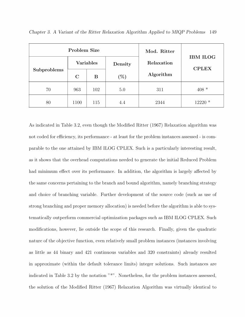
Chapter 3. A Variant of the Ritter Relaxation Algorithm Applied to MIQP Problems 149
Problem Size Mod. Ritter
Relaxation
Algorithm
IBM ILOG
CPLEXSubproblems
Variables Density
C B (%)
70 963 102 5.0 311 408 *
80 1100 115 4.4 2344 12220 *
As indicated in Table 3.2, even though the Modified Ritter (1967) Relaxation algorithm was
not coded for efficiency, its performance - at least for the problem instances assessed - is com-
parable to the one attained by IBM ILOG CPLEX. Such is a particularly interesting result,
as it shows that the overhead computations needed to generate the initial Reduced Problem
had minimum effect over its performance. In addition, the algorithm is largely affected by
the same concerns pertaining to the branch and bound algorithm, namely branching strategy
and choice of branching variable. Further development of the source code (such as use of
strong branching and proper memory allocation) is needed before the algorithm is able to sys-
tematically outperform commercial optimization packages such as IBM ILOG CPLEX. Such
modifications, however, lie outside the scope of this research. Finally, given the quadratic
nature of the objective function, even relatively small problem instances (instances involving
as little as 44 binary and 421 continuous variables and 320 constraints) already resulted
in approximate (within the default tolerance limits) integer solutions. Such instances are
indicated in Table 3.2 by the notation ”*”. Nonetheless, for the problem instances assessed,
the solution of the Modified Ritter (1967) Relaxation Algorithm was virtually identical to

Chapter 3. A Variant of the Ritter Relaxation Algorithm Applied to MIQP Problems 150
the one of IBM ILOG CPLEX and often obtained under faster computation times, thus
clearly demonstrating its viability for solving solving large, bordered-structure optimization
problems. The next section summarizes the findings of this paper and lists directions for
future research.
3.4 Conclusions and Future Research
This paper presents an extension of the Ritter (1967) Relaxation Algorithm for solving
bordered-structure problems with linear, integer, or mixed-integer subproblems and with
linear or quadratic objective functions. In summary, the algorithm relaxes some of the non-
negativity and integer restrictions in order to produce a smaller and easier to solve problem,
namely the Reduced Problem. In the original algorithm, the relaxed non-negativity restric-
tions are enforced sequentially either by swapping decision variables between the relaxed
and non-relaxed sets (and recomputing the Reduced Problem parameters) or by adding new
constraints to the Reduced Problem. The algorithm terminates once the optimum solution
to the Reduced Problem also satisfies the non-negativity restriction of all relaxed variables.
The proposed variation is similar to the original Ritter (1967) Relaxation Algorithm, except
that it does not allow swapping of decision variables between the relaxed and non-relaxed
sets. Hence, the modified algorithm relies solely on the inclusion of constraints into the
Reduced Problem in order to enforce the non-negativity (and, now, the integer restriction)
of the relaxed variables. By preventing the swapping operation from taking place, the mod-

Chapter 3. A Variant of the Ritter Relaxation Algorithm Applied to MIQP Problems 151
ified algorithm requires fewer matrix manipulations and fewer numerical comparisons, and,
thus, has improved numerical stability. Perhaps even more important, given the dichoto-
mous nature of the added constraints, it is shown that the algorithm can be combined with
the branch and bound algorithm in order to solve problems with integer or mixed-integer
subproblems.
However, considerable research is needed before such an algorithm is able to systematically
outperform commercial optimization packages such as IBM ILOG CPLEX. First, the same
concerns pertaining to the branch and bound algorithm, namely branching strategy and
choice of branching variable, also apply to the proposed algorithm. In addition, since a
considerable amount of computational effort is dedicated to the generation of constraints
enforcing the branching and the upper and lower bound restrictions, and since these are
incorporated sequentially into the Reduced Problem, it may be possible to further improve
the efficiency of the algorithm by the concomitant use of Gomory cuts. Alternatively, since
the branch and bound computations are so demanding, it may be advantageous to generate
and add all boundary restrictions to the Reduced Problem a priori, thus ensuring that each
subproblem generated enforces, at least, the LP relaxation of the original problem. Finally,
since the algorithm is designed for bordered-structure problems, it may be applicable to
seemingly structureless problems, but which can be mapped into an structured problem
through rearrangement of their constraint coefficients. See Aykanat et al. (2004), Duff and
Scott (2005), Ferris and Horn (1998), Fragniere et al. (2000), Pinar and Aykanat (1996), and
Pinar et al. (1996) for different algorithms to reorganize the coefficients of the constraint
Chapter 3. A Variant of the Ritter Relaxation Algorithm Applied to MIQP Problems 152
matrix into exploitable structures.
3.5 Appendix
This section presents the mathematical proofs of the propositions introduced in Section 3.2.
Proof of Proposition 3.1. Let XO be the original problem feasible region and let X 1R be
the Reduced Problem feasible region generated on the first iteration of the Modified Ritter
(1967) Relaxation Algorithm, that is, let:
XO ≡{x ∈ (R+ × Z+)
∣∣∣∣∣Bjxj +Djxp+1 = bj, ∀ j = 1, · · · , p,p∑
j=1
Aeqj xj +Deq xp+1 = beq,
p∑
j=1
Aineqj xj +Dineq xp+1 ≤ bineq
}
X 1R ≡
{xj2, ∀ j = 1, · · · , p, xp+1 ∈ (R+ × Z+)
∣∣∣∣∣
p∑
j=1
Fjxj2 + Fp+1xp+1 = f,
p∑
j=1
Gjxj2 +Gp+1xp+1 ≤ g,
p∑
j=1
|Sj2|∑
i=1
xij2 +
np+1∑
i=1
xip+1 ≤M
,
Where the notation (R+ × Z+) indicates the non-negative, mixed-integer nature of the
problem. For simplicity, the slack variables (if any) used to place constraint Bjxj +
Djxp+1 = bj in standard form are grouped with xj, j = 1, · · · , p. Let M be a sufficiently
large, positive constant preventing X 1R from being unbounded. Now, using the parame-
ter substitutions (3.13) and some rearrangement of the terms, constraint∑p
j=1 Fjxj2 +
Fp+1xp+1 = f can be rewritten as∑p
j=1
(Aeqj1
(bj −Bjxj2 −Djxp+1
)+ Aeqj2 xj2
)+
Deq xp+1 = beq and constraint∑p
j=1Gjxj2 + Gp+1xp+1 ≤ g can be rewritten as
Chapter 3. A Variant of the Ritter Relaxation Algorithm Applied to MIQP Problems 153
∑pj=1
(Aineqj1
(bj −Bjxj2 −Djxp+1
)+ Aineqj2 xj2
)+ Dineq xp+1 ≤ bineq. After employ-
ing the variable substitution (3.11) and realizing that xj1 and xj2, are mutually exclusive
partitions of the jth subproblem decision variables, it follows that:
XO ∩
xj2, ∀ j = 1, · · · , p, xp+1 ∈ R
∣∣∣∣∣∣
p∑
j=1
|Sj2|∑
i=1
xij2 +
np+1∑
i=1
xip+1 ≤M
=
X 1R ∩ {xj1 ∈ (R+ × Z+), ∀ j = 1, · · · , p}
Now, since the original problem feasible region is bounded, any partial summation of
its decision variables is finite. Consequently, for M sufficiently large, the constraint
∑pj=1
∑|Sj2|i=1 xij2 +
∑np+1
i=1 xip+1 ≤ M is redundant to the original problem, that is: XO ∩
{xj2, ∀ j = 1, · · · , p, xp+1 ∈ R|∑pj=1
∑|Sj2|i=1 xij2 +
∑np+1
i=1 xip+1 ≤ M} = XO. As a result,
XO = X 1R ∩ {xj1 ∈ (R+ × Z+), ∀ j = 1, · · · , p} ⇒ XO ⊆ X 1
R.
Proof of Corollary 3.1. Let XO and X 1R be defined as in the proof of Proposition 3.1, and let
Nε(0) be a sufficiently small ε-neighborhood around the origin. For notational simplicity, let
Q ≡ {xj2, ∀ j = 1, · · · , p, xp+1 ∈ R|∑pj=1
∑|Sj2|i=1 xij2 +
∑np+1
i=1 xip+1 ≤M} and let R ≡ {xj1 ∈
(R+ × Z+), ∀ j = 1, · · · , p}, that is, let Q be the polyhedral set preventing X 1R from being
unbounded and let R be the polyhedral set corresponding to the non-negativity and integer
restrictions, if any, of the relaxed decision variables. Now, since XO is unbounded and since
X 1R is bounded, in general, XO 6⊆ X 1
R. However, since X 1R is a relaxation of XO, it remains true
that (XO ∩Q) = (X 1R ∩R), and, thus, that (XO ∩Nε(0) ∩Q) = (X 1
R ∩Nε(0) ∩R). However,
for ε sufficiently small, Nε(0) = (Nε(0) ∩Q) and X 1R = (X 1
R ∩Nε(0)). Therefore:
(XO ∩Nε(0) ∩Q) =(X 1R ∩Nε(0) ∩R
)

Chapter 3. A Variant of the Ritter Relaxation Algorithm Applied to MIQP Problems 154
⇒ (XO ∩Nε(0)) =(X 1R ∩R
)
⇒ (XO ∩Nε(0)) ⊆ X 1R.
Proof of Corollary 3.2. Let XO and X 1R be defined as in the proof of Proposition 3.1, let
Nε(0) be a sufficiently small ε-neighborhood around the origin, and let yO be the optimum
solution to the original problem. If XO is bounded, then, by Proposition 3.1, XO ⊆ X 1R.
Consequently, yO ∈ XO ⇒ yO ∈ X 1R. Conversely, if XO is unbounded, then, by Corollary 3.1,
(XO ∩Nε(0)) ⊆ X 1R. Since yO is finite, yO ∈ Nε(0). Together, yO ∈ XO, yO ∈ Nε(0)⇒ yO ∈
(XO ∩Nε(0))⇒ yO ∈ X 1R.
Proof of Corollary 3.3. Let XO and X 1R be defined as in the proof of Proposition 3.1,
and let yO and y1R denote, respectively, the optimum solution to the original and to the
initial Reduced Problem. First, note that (3.7) ensures that X 1R is bounded. Now, from
Corollary 3.2, yO ∈ XO ⇒ yO ∈ X 1R ⇒ X 1
R 6= ∅. Since the Reduced Problem is non-empty
and bounded, it must have a finite optimum solution y1R. Observe that no restrictions on
the uniqueness of yO and y1R are imposed. In addition, the converse relationship may not be
true, that is, y1R ∈ X 1
R 6⇒ y1R ∈ XO, since, in general, X 1
R 6⊆ XO. Hence, it is possible for the
initial Reduced Problem to have an optimum solution, but for such solution to violate the
non-negativity and/or integer restriction of some of the relaxed variables.
Proof of Proposition 3.2. Let XO and yO be, respectively, the feasible region of the
original problem and its optimum solution; and let X kR and ykR be, respectively, the feasible
region of the Reduced Problem solved on the kth iteration of the Modified Ritter (1967)

Chapter 3. A Variant of the Ritter Relaxation Algorithm Applied to MIQP Problems 155
Relaxation Algorithm and its optimum solution. Here, it is shown that ykR ∈ XO ⇔ ykR
incumbent:
(=⇒) If ykR ∈ XO, then ykR satisfies all constraints of the original problem, including those
that have been relaxed in the Reduced Problem. As per Step 13 of the Modified Ritter
(1967) Relaxation Algorithm, the Reduced Problem is fathomed, and ykR is saved as
an incumbent solution.
(⇐=) Here, the contrapositive is proven, that is, it is shown that an optimum solution
to the Reduced Problem that is not feasible to the original problem cannot be an
incumbent solution to the Modified Ritter (1967) Relaxation Algorithm. Suppose
that ykR 6∈ XO. Since ykR ∈ X kR, it follows that ykR satisfies all constraints of the
current Reduced Problem, and, thus, that it satisfies all constraints in the original
problem except, perhaps, for some integer and/or boundary restrictions which have
been relaxed. In fact, since ykR ∈ X kR, but ykR 6∈ XO, at least one of its components,
say the ith element of the jth subproblem, must violate some of these restrictions (e.g.,
xij1 < 0 or xij1 6∈ Z). Observe that the violated element cannot be a decision variable in
the non-relaxed partition (i.e., xj2, j = 1, · · · , p) or in the set of complicating variables
(i.e., xp+1), as, otherwise, ykR 6∈ X kR. Now, if a boundary restriction is violated, for
instance if xij1 < 0, then constraint {Bj}i xj2 + {Dj}i xp+1 ≤ {bj}i is added to the
Reduced Problem and such is reoptimized as per Steps 10 and 12 of the Modified
Ritter (1967) Relaxation Algorithm. Conversely, if an integer restriction is violated,
for instance if xij1 = a, where a is some fractional value, then the algorithm removes

Chapter 3. A Variant of the Ritter Relaxation Algorithm Applied to MIQP Problems 156
the current Reduced Problem from set NL and adds two new Reduced Problems, each
one with a mutually exclusive constraint: −{Bj}i xj2 − {Dj}i xp+1 ≤ bac − {bj}i and
{Bj}i xj2 + {Dj}i xp+1 ≤ −dae + {bj}i as per Step 14 of the Modified Ritter (1967)
Relaxation Algorithm. Whichever the case, such violations trigger the inclusion of
additional constraints that eliminate ykR from the feasible region of the new Reduced
Problem(s). Therefore, ykR cannot be an incumbent solution to the algorithm.
Proof of Proposition 3.3. Let XO, X kR and yO be defined as in the proof of Proposition
3.2. First, from Corollary 3.2, if yO exists, then yO ∈ X 1R. Therefore, at least on the
first iteration of the Modified Ritter (1967) Relaxation Algorithm, the feasible region of the
Reduced Problem contains the optimum solution to the original problem. Since the algorithm
performs a dichotomous, exhaustive search following a scheme similar to the branch and
bound algorithm, on its kth iteration, either the optimum solution to the original problem
has already been identified and saved as an incumbent solution or at least one of the Reduced
Problems maintain the optimum solution to the original problem within its feasible region.
Since the algorithm terminates in a finite number of iterations, as it will be shown in the proof
of Proposition 3.4, it will eventually identify the optimum solution to the original problem
as an incumbent solution. Finally, since, by Proposition 3.2, all incumbent solutions are
feasible to the original problem, since the transformations used to generate the Reduced
Problem do not alter the objective function of the original problem (other than reducing its
dimensionality), and since the algorithm outputs the one with the best objective function
value, it follows that the Modified Ritter (1967) Relaxation Algorithm will always identify

Chapter 3. A Variant of the Ritter Relaxation Algorithm Applied to MIQP Problems 157
the optimum solution to the original problem if one exists.
Proof of Proposition 3.4. As shown in the proof of Proposition 3.3, a new iteration of
the modified algorithm takes place whenever one of the relaxed variables, say the ith element
of the jth subproblem, violates a boundary or integer restriction (e.g., xij1 < 0 or xij1 6∈ Z).
Since such violations are eliminated via the inclusion of extra constraints in the Reduced
Problem, since such constraints are only removed when they become redundant, and since
there is a finite number of such possible constraints (as there are a finite number of elements
in set xj1, j = 1, · · · , p; as the algorithm employs a dichotomous search strategy; and as
the feasible region of the Reduced Problem is bounded), it follows that the algorithm must
terminate in a finite number of iterations.
Chapter 4
The Dynamic Bus Evacuation
Problem with Stochastic Customers
and Demand
158
Chapter 4. The Dynamic BEP with Stochastic Customers and Demand 159
The Dynamic Bus Evacuation Problem with Stochastic
Customers and Demand
Victor C. Pereira and Douglas R. Bish
(ABSTRACT)
This research introduces a two-stage stochastic formulation and an iterative (dynamic) algo-
rithm for the Bus Evacuation Problem, a unique Vehicle Routing Problem motivated both
by its humanitarian significance and by the challenges of planning and implementing transit-
based, regional evacuations. In this problem, a fleet of capacitated buses must transport all
transit-dependent individuals from a set of pick-up locations to a depot/shelter with min-
imum total travel time. The problem assumes that a set of possible demand scenarios is
available, and that the exact number of evacuees on each location, if any, becomes known
once a bus visits it for the first time. The effect of exploratory visits (sampling) and symme-
try is explored, and the resulting insights used to develop a deterministic formulation for the
problem. While, at least in a dynamic context, these formulations are equivalent, the de-
terministic variation has considerably improved tractability, preserves the desired sampling
behavior, and employs constraints that break some of the problem symmetries in favor of arc
traversals leading to reduced total travel times. Although this research focuses on evacua-
tion planning/implementation, the concepts herein developed are readily applicable to other
transportation settings such as supply deployment and search and rescue operations.
Keywords: Evacuation Planning; Dynamic Vehicle Routing Problem; Stochastic

Chapter 4. The Dynamic BEP with Stochastic Customers and Demand 160
Programming; Uncertain Demand
Acknowledgments: This work has been supported by the National Science Foundation
under Award Number 1055360.
4.1 Introduction
The Bus Evacuation Problem (BEP) is a variant of the Vehicle Routing Problem (VRP),
where a fleet of capacitated buses, initially parked at a depot, must transport transit-
dependent individuals from a set of predetermined pick-up locations to one or more shelters.
The problem arises in regional evacuation settings, where some of the residents either lack
reliable means of personal transportation, as in the evacuation of New Orleans preceding the
landfall of Hurricane Katrina, or lack enough time for alternative evacuation methods, such
as in the evacuation of urban clusters facing bomb threats.
This research presents and analyzes a two-stage stochastic formulation for the BEP in which
the number of evacuees on each pick-up location, if any, is revealed dynamically during
the course of the evacuation. The problem forces every evacuee to be transported to a
depot/shelter, while minimizing the expected total travel time of a homogeneous fleet of
buses. The first stage of the proposed stochastic formulation identifies the subsequent arc
traversal for each vehicle, whereas the second stage identifies their remaining arc traversals
provided a set of equal-probability scenarios. In this research, the term scenario refers to a
set of potential demand realizations, one value for each pick-up location. Consequently, the
Chapter 4. The Dynamic BEP with Stochastic Customers and Demand 161
problem does not require demands to be independent of each other, an important distinction
from most of the stochastic VRP literature. In addition, it is assumed that all evacuees are
waiting at these locations at the onset of the evacuation. These, however, are not explicitly
modeled. Instead, demands are treated as a percentage (possibly multiples) of the vehicle
capacity. The problem assumes that the exact number of evacuees (or, rather, full bus
loads) waiting on each pick-up location is only revealed after a vehicle visits it for the first
time. A iterative algorithm, which reoptimizes the problem as new information becomes
available, is presented. Finally, structural properties of the problem, namely sampling and
symmetry, are identified and used to generate an alternative, deterministic formulation, able
to attain better solutions under considerably smaller computation times. Sampling refers
to exploratory visits to pick-up locations aiming to ascertain its demand, and, thus, to
eliminate future round trips between said location and the depot. Symmetry refers to the
problem default inability to distinguish between seemingly identical arc traversals, but which
may result in distinct objective function values depending on the realized demands at the
destination nodes.
The modeling and optimization literature on transit-based evacuation planning/implemen-
tation is scarce and fairly recent. In fact, with the exception of Goerigk and Grun (2012),
Kulshrestha et al. (2012), and Song et al. (2009), no related literature accounting for the
stochastic nature of evacuee demand has been located. Goerigk and Grun (2012) propose
a deterministic and a stochastic formulation with no recourse for the BEP, both seeking
to minimize the longest travel time across vehicles (a proxy for the evacuation completion

Chapter 4. The Dynamic BEP with Stochastic Customers and Demand 162
time). Similar to the proposed formulation, the authors do not explicitly model evacuees,
treating demands as a function of the vehicle capacity. Vehicles, initially parked at a depot,
travel to the various pick-up locations, and, from there, back and forth between pick-up
locations and shelters until each location has been visited enough times to accommodate all
its evacuees. Their stochastic formulation seeks to balance the number of buses that depart
immediately with those that remain stationed at the depot until the number of evacuees
on each pick-up location becomes known. Kulshrestha et al. (2012) propose and analyze a
stochastic, Location Routing Problem (LRP) formulation for the BEP that minimizes the
expected total travel time of the fleet. In their formulation, vehicles are initially assigned
one of the possible pick-up locations, and, from there, they perform round trips to a set of
capacitated shelters until either all demand is satisfied or a limiting travel time is reached.
Although their formulation is conceptually similar to the one proposed by Goerigk and Grun
(2012), it differs in one important aspect: vehicles are not allowed to move to a different
pick-up location once they finish rescuing all evacuees from their initial assignment. In ad-
dition, while the problem assumes that a set of scenarios is provided, it limits the number
of pick-up locations which demands can differ from the expected value. Finally, Song et al.
(2009) propose a stochastic, LRP formulation for the BEP that incorporates a reliability
constraint (based on the logistic distribution) to account for the uncertainty on the number
of transit-dependent evacuees on each pick-up location. Their formulation enforces strict
pick-up time windows, but assumes that all evacuees are at the pick-up locations at the
onset of the evacuation. In addition, a maximum travel time per vehicle is enforced as a

Chapter 4. The Dynamic BEP with Stochastic Customers and Demand 163
proxy for the overall completion time of the evacuation. Their formulation simultaneously
seeks the set of uncapacitated shelters that must open and the corresponding routes for a
fleet of capacitated vehicles that minimize their total travel time.
The stochastic formulation presented in this research shares several commonalities with the
ones proposed by Kulshrestha et al. (2012) and, in particular, by Goerigk and Grun (2012).
However, there are some important differences. First, both studies assume that vehicles
can only perform round trips between pick-up locations and shelters, whereas the proposed
formulation assumes a complete network. Second, the formulation proposed by Goerigk
and Grun (2012) assumes that the amount of time that vehicles must wait at the depot for
additional information is a known problem parameter, whereas, in the proposed formulation,
the realized demand on each pick-up location only becomes available once a bus visits it for
the first time. Third, both studies assume that vehicles cannot be rerouted, whereas the
proposed solution methodology reoptimizes the problem as additional information becomes
available. Finally, both studies assume independence of the possible demand realizations,
whereas the proposed formulation does not.
In summary, the proposed formulation can be classified as a two-stage stochastic Dynamic
Vehicle Routing Problem (D-VRP) with stochastic customers and demands, that is a D-VRP
which relies on the known stochastic nature of demands to identify improved routes for the
fleet and which considers the possibility that some of these demands equal zero. Although
the assumption of zero-demand at any pick-up location may not seem realistic for most real-
world evacuation settings, it is well suited for modeling LRP variations of the BEP, such as
Chapter 4. The Dynamic BEP with Stochastic Customers and Demand 164
the ones proposed by Kulshrestha et al. (2012) and Song et al. (2009).
The origins of the D-VRP can be traced to Wilson and Colvin (1977), who propose a variation
of the Dial-A-Ride Problem in which customer requests for trips arrive dynamically (i.e., after
vehicles begun their tour). According to Pillac et al. (2013), unlike traditional VRPs, the D-
VRP is based on the premise that either the problem parameters change or their uncertainty
is resolved after the originally planned tours start to be implemented. Consequently, the
D-VRP allows factors initially unknown to the planner to be incorporated into the final
solution, thus potentially reducing operational costs, improving customer service, and even
reducing environmental impact (Pillac et al., 2013). Since the originally planned routes must
be reoptimized to account for the new information, the D-VRP consists of a sequence of static
VRPs (see Larsen et al., 2007; Pillac et al., 2013, for a comprehensive review of the D-VRP
literature). Among its many variations, the proposed formulation more closely resembles the
stochastic D-VRP. Such variant is similar to its deterministic counterpart in the sense that
some of the parameters (in this case, the number of full bus loads needed to accommodate
every evacuee waiting at a pick-up location) are unknown a priori and reveled dynamically
during the implementation of the routes (in this case, as vehicles visit the pick-up locations
for the first time). However, contrary to its deterministic counterpart, the problem exploits
the known stochastic nature of demands to determine the arc traversals more likely to result
in better objective function values.
Although the D-VRP literature is extensive, its application to humanitarian logistics is some-
what scarce. In fact, no literature specifically focusing on transit-based evacuation planning
Chapter 4. The Dynamic BEP with Stochastic Customers and Demand 165
was located. Brotcorne et al. (2003) and Gendreau et al. (2001) propose a D-VRP for-
mulation for ambulance relocation during disaster relief operations, whereas Haghani and
Yang (2007) and Yi and Ozdamar (2007) propose a D-VRP formulation for supply deploy-
ment during such operations. Finally, Fajardo and Waller (2012) introduce and analyze a
single-vehicle, uncapacitated Stochastic Dynamic Traveling Salesman Problem (D-TSP) for-
mulation for rescuing disaster victims whose number and position is unknown a priori. Their
formulation shares several commonalities with the proposed BEP variation. First, their for-
mulation assumes that a set of pick-up locations (i.e., a list of potential victim positions) and
a set of potential demands within each location are provided. Second, the realized demand
on each location (i.e., whether any victims are present or not) only becomes known upon vi-
sual observation, that is, once vehicles visit the location for the first time. Third, the authors
also propose a two-stage stochastic formulation, where, on the first stage, the subsequent arc
traversal for the vehicle is identified, and, on the second stage, the remaining arc traversals
leading it back to the depot under each possible demand realization are identified. Finally,
their formulation also seeks to minimize the expected total travel time, as a function of the
demand probabilities. Despite these similarities, their formulation differs from the proposed
BEP variation in some important aspects. First, the authors modeled the problem as a
D-TSP. Consequently, efficiencies from using multiple vehicles and from allowing vehicles
to return to the depot to unload evacuees (or disaster victims) multiple times are ignored.
Second, their formulation focuses on search-and-rescue operations. Consequently, it ignores
vehicle capacity restrictions and the possibility of split deliveries, important considerations
Chapter 4. The Dynamic BEP with Stochastic Customers and Demand 166
on a evacuation setting. Finally, and more importantly, while the authors mention the po-
tential benefits of sampling and symmetry, their formulation does not explicitly integrate
these features in order to identify improved routes for the fleet.
In summary, the contributions of this paper are: (i) introduction of a dynamic, two-stage
stochastic formulation that extends the BEP to the case of uncertain demand; (ii) develop-
ment of an algorithm that iteratively solves the problem as additional information becomes
available; (iii) examination of the effect of sampling (i.e., the use of exploratory visits to de-
termine the demand on each pick-up location) and symmetry over the expected total travel
time of the fleet; and (iv) development of an alternative, deterministic formulation that in-
corporates these insights to attain better routes for the fleet while considerably improving
the problem tractability. Observe that the concepts herein developed are readily applicable
to any other mass transit vehicle, and, possibly, to alternative VRP settings such as supply
deployment and search and rescue operations.
This paper is organized as follows: Section 4.2 presents the proposed formulation and an
iterative algorithm that reoptimizes the problem as additional information becomes available;
Section 4.3 explores the effect of sampling and symmetry over the expected total travel time
of the fleet and uses these insights to develop an improved formulation for the problem; and,
finally, Section 4.4 summarizes the main findings of this paper and lists the future work
needed on the area.
Chapter 4. The Dynamic BEP with Stochastic Customers and Demand 167
4.2 Modeling Framework
This section presents the modeling notation, a two-stage stochastic D-VRP formulation for
the BEP with stochastic customers and demand, an upper bound on the maximum number
of arc traversals per vehicle (a support parameter used within the proposed formulation),
and an iterative algorithm that reoptimizes the problem as additional information becomes
available.
Consider the complete, directed network (N,A), where N and A represent the set of nodes
and arcs, respectively. The set N consists of set P , the set of pick-up locations (each one
serving a neighborhood requiring evacuation services), and node 0, the depot, which also
functions as a shelter. Each arc (i, j) ∈ A has an associated arc traversal time, tij, satisfying
the triangle inequality, that is, tij ≤ tik + tkj, ∀ (i, j), (i, k), and (k, j) ∈ A. For simplicity,
let tij = tji, ∀ i, j ∈ N . In addition, let S be the set of possible scenarios, let P ∗ be the
set of pick-up locations with uncertain demand (i.e., not yet visited by any vehicle), let R∗
be the set of previously traversed arcs, and let C∗ be the set of previously performed pick-
ups. Finally, let Dsj be the total demand of node j under scenario s, let V be the number
of available buses, and let T be the maximum number of arc traversals per vehicle. The
decision variables, objective function, and constraint set for the problem are as follows:
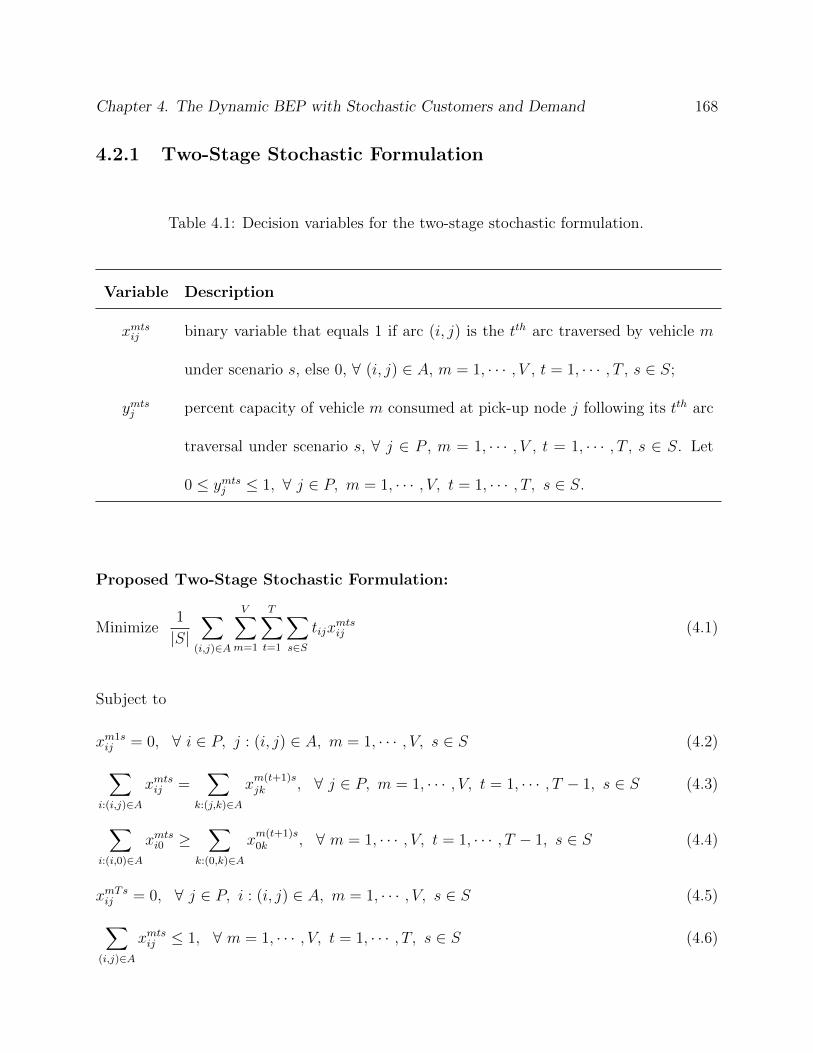
Chapter 4. The Dynamic BEP with Stochastic Customers and Demand 168
4.2.1 Two-Stage Stochastic Formulation
Table 4.1: Decision variables for the two-stage stochastic formulation.
Variable Description
xmtsij binary variable that equals 1 if arc (i, j) is the tth arc traversed by vehicle m
under scenario s, else 0, ∀ (i, j) ∈ A, m = 1, · · · , V , t = 1, · · · , T , s ∈ S;
ymtsj percent capacity of vehicle m consumed at pick-up node j following its tth arc
traversal under scenario s, ∀ j ∈ P , m = 1, · · · , V , t = 1, · · · , T , s ∈ S. Let
0 ≤ ymtsj ≤ 1, ∀ j ∈ P, m = 1, · · · , V, t = 1, · · · , T, s ∈ S.
Proposed Two-Stage Stochastic Formulation:
Minimize1
|S|∑
(i,j)∈A
V∑
m=1
T∑
t=1
∑
s∈S
tijxmtsij (4.1)
Subject to
xm1sij = 0, ∀ i ∈ P, j : (i, j) ∈ A, m = 1, · · · , V, s ∈ S (4.2)
∑
i:(i,j)∈A
xmtsij =∑
k:(j,k)∈A
xm(t+1)sjk , ∀ j ∈ P, m = 1, · · · , V, t = 1, · · · , T − 1, s ∈ S (4.3)
∑
i:(i,0)∈A
xmtsi0 ≥∑
k:(0,k)∈A
xm(t+1)s0k , ∀ m = 1, · · · , V, t = 1, · · · , T − 1, s ∈ S (4.4)
xmTsij = 0, ∀ j ∈ P, i : (i, j) ∈ A, m = 1, · · · , V, s ∈ S (4.5)
∑
(i,j)∈A
xmtsij ≤ 1, ∀ m = 1, · · · , V, t = 1, · · · , T, s ∈ S (4.6)

Chapter 4. The Dynamic BEP with Stochastic Customers and Demand 169
ymtsj ≤∑
i:(i,j)∈A
xmtsij , ∀ j ∈ P, m = 1, · · · , V, t = 1, · · ·T, s ∈ S (4.7)
∑
j∈P
t∑
l=1
ymlsj −∑
i:(i,0)∈A
t∑
l=1
xmlsi0 ≤ 1, ∀ m = 1, · · · , V, t = 1, · · · , T, s ∈ S (4.8)
V∑
m=1
T∑
t=1
ymtsj = Dsj , ∀ j ∈ P, s ∈ S (4.9)
xmtsij = xmtuij , ∀ (i, j) ∈ A, m = 1, · · · , V, t = t∗, s ∈ S, u ∈ S, s 6= u (4.10)
∑
i:(i,j)∈A
V∑
m=1
T∑
t=1
xmtsij ≥ 1, ∀ j ∈ P, s ∈ S (4.11)
xmtsij = 1, ∀ {(i, j),m, t} ∈ R∗, s ∈ S (4.12)
ymtsj = g, ∀ {j,m, t, g} ∈ C∗, s ∈ S. (4.13)
Objective Function (4.1) minimizes the expected total travel time of the fleet assuming that
all scenarios have equally likely probability of realization. Constraints (4.2)-(4.6) prevent
the construction of invalid routes, including the elimination of subtours. Constraint (4.2)
prevents buses from starting their tour from a pick-up location. If a vehicle’s tth arc traversal
ends at a pick-up location, then (4.3) forces the vehicle’s (t+ 1)th arc traversal to start from
such location. Constraint (4.4) is similar to (4.3), but it allows a vehicle’s final arc traversal
to end at the depot. Constraint (4.5) forces the vehicle’s T th arc traversal, if used, to end at
the depot, and (4.6) limits vehicles to one arc traversal a time. Constraints (4.7)-(4.9) enforce
the vehicle capacity restrictions. Constraint (4.7) prevents evacuees from boarding a transit
vehicle unless such is visiting their respective pick-up location; (4.8) enforces the bus capacity
restriction, allowing for multiple drop-offs at the depot; and (4.9) ensures that the demand
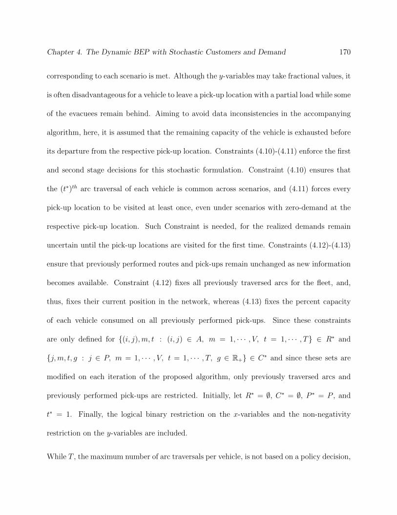
Chapter 4. The Dynamic BEP with Stochastic Customers and Demand 170
corresponding to each scenario is met. Although the y-variables may take fractional values, it
is often disadvantageous for a vehicle to leave a pick-up location with a partial load while some
of the evacuees remain behind. Aiming to avoid data inconsistencies in the accompanying
algorithm, here, it is assumed that the remaining capacity of the vehicle is exhausted before
its departure from the respective pick-up location. Constraints (4.10)-(4.11) enforce the first
and second stage decisions for this stochastic formulation. Constraint (4.10) ensures that
the (t∗)th arc traversal of each vehicle is common across scenarios, and (4.11) forces every
pick-up location to be visited at least once, even under scenarios with zero-demand at the
respective pick-up location. Such Constraint is needed, for the realized demands remain
uncertain until the pick-up locations are visited for the first time. Constraints (4.12)-(4.13)
ensure that previously performed routes and pick-ups remain unchanged as new information
becomes available. Constraint (4.12) fixes all previously traversed arcs for the fleet, and,
thus, fixes their current position in the network, whereas (4.13) fixes the percent capacity
of each vehicle consumed on all previously performed pick-ups. Since these constraints
are only defined for {(i, j),m, t : (i, j) ∈ A, m = 1, · · · , V, t = 1, · · · , T} ∈ R∗ and
{j,m, t, g : j ∈ P, m = 1, · · · , V, t = 1, · · · , T, g ∈ R+} ∈ C∗ and since these sets are
modified on each iteration of the proposed algorithm, only previously traversed arcs and
previously performed pick-ups are restricted. Initially, let R∗ = ∅, C∗ = ∅, P ∗ = P , and
t∗ = 1. Finally, the logical binary restriction on the x-variables and the non-negativity
restriction on the y-variables are included.
While T , the maximum number of arc traversals per vehicle, is not based on a policy decision,
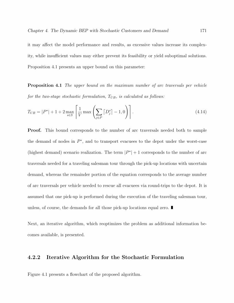
Chapter 4. The Dynamic BEP with Stochastic Customers and Demand 171
it may affect the model performance and results, as excessive values increase its complex-
ity, while insufficient values may either prevent its feasibility or yield suboptimal solutions.
Proposition 4.1 presents an upper bound on this parameter:
Proposition 4.1 The upper bound on the maximum number of arc traversals per vehicle
for the two-stage stochastic formulation, TUB, is calculated as follows:
TUB = |P ∗|+ 1 + 2 maxs∈S
⌈1
Vmax
(∑
j∈P
⌈Dsj
⌉− 1, 0
)⌉. (4.14)
Proof. This bound corresponds to the number of arc traversals needed both to sample
the demand of nodes in P ∗, and to transport evacuees to the depot under the worst-case
(highest demand) scenario realization. The term |P ∗|+ 1 corresponds to the number of arc
traversals needed for a traveling salesman tour through the pick-up locations with uncertain
demand, whereas the remainder portion of the equation corresponds to the average number
of arc traversals per vehicle needed to rescue all evacuees via round-trips to the depot. It is
assumed that one pick-up is performed during the execution of the traveling salesman tour,
unless, of course, the demands for all those pick-up locations equal zero.
Next, an iterative algorithm, which reoptimizes the problem as additional information be-
comes available, is presented.
4.2.2 Iterative Algorithm for the Stochastic Formulation
Figure 4.1 presents a flowchart of the proposed algorithm.

Chapter 4. The Dynamic BEP with Stochastic Customers and Demand 172
Initialization: t∗ ← 1, C∗ ← ∅, R∗ ← ∅, P ∗ ← P, T ← TUB
Optimize Problemt∗ ← t∗ + 1
For (i, j) ∈ A,m = 1, · · · , V
xmt∗1ij = 1?
R∗ ← R∗ ∪ {(i, j),m, t∗}
j ∈ P ∗?j ∈ P?
C∗ ← C∗ ∪ {j,m, t∗, ymt∗1j }
For s ∈ SP ∗ ← P ∗ − {j}
Dsj = D∗
j ?Dsj ← D∗
j
C∗ ← C∗ ∪ {j,m, t∗, ymt∗sj }
P ∗ = ∅?
Terminate.Solution is Final.
loopexit
no
yes
no
yes
no
yes
no
yes
exit loop
no
yes
Figure 4.1: Flowchart of the iterative algorithm for the stochastic formulation.
Chapter 4. The Dynamic BEP with Stochastic Customers and Demand 173
The algorithm proceeds as follows. First, the parameters t∗, C∗, R∗, and P ∗ are initialized.
Recall that t∗ corresponds to the first stage decision of the stochastic formulation, that is,
to the subsequent arc traversal of each vehicle; that C∗ corresponds to the set of previously
performed pick-ups; and that R∗ corresponds to the set of previously traversed arcs. The
parameter P ∗ is not part of the two-stage stochastic formulation, but corresponds to the set
of pick-up locations that have not yet been visited, and, thus, that have uncertain demand.
Since the demands on each pick-up location are updated as additional information becomes
available, the upper bound on the maximum number of arc traversals per vehicle, TUB,
decreases monotonically with t∗ (except, of course, when the worst-case scenario is realized, in
which case TUB remains unchanged). Consequently, the initial TUB-parameter is sufficiently
large for all iterations of the algorithm, and does not need to be recomputed in order to
prevent conflicts with previously added elements in C∗ and R∗. Now, on each iteration of
the algorithm, the problem is reoptimized; the (t∗)th arc traversal of each vehicle, if any, is
saved into set R∗; and its percent capacity consumed at the destination node (if such is a
pick-up location) is saved into set C∗. If the destination node is a pick-up location that has
not yet been visited, then such is removed from set P ∗ and all its scenarios updated with
its realized demand, D∗j . Unfortunately, unrealized scenarios cannot be removed from the
problem parameter set in order to maintain the integrity of the decision variables indexes.
Although somewhat inefficient, by updating the value of all non-realized demands to D∗j ,
the algorithm ensures that future pick-ups at this pick-up location meet its realized demand
regardless of the scenario realizations at alternative pick-up locations. If all pick-up locations

Chapter 4. The Dynamic BEP with Stochastic Customers and Demand 174
have been visited (i.e., if P ∗ = ∅), then, after one last optimization, the solution attained is
final and the algorithm terminates. Otherwise, t∗ is incremented by one and a new iteration is
performed. Example 4.1 shows the implementation of the algorithm for an example network
with three pick-up locations and three scenarios.
Example 4.1 Consider the example network presented in Figure 4.2. Observe that the
network is a complete digraph with symmetrical arc traversal times that satisfy the triangle
inequality. For simplicity, let V = 1 bus. Suppose that there are three possible scenarios:
scenario 1 has D11 = 1, D1
2 = 1, and D13 = 1; scenario 2 has D2
1 = 0, D22 = 1, and D2
3 = 2;
and scenario 3 has D31 = 0, D3
2 = 2, and D33 = 1.
2
1
2
0
3
2
3
3
2
2
Figure 4.2: An example network for the algorithm implementation.
Naturally, the optimal solution for this problem is trivial under the assumption of perfect
information, that is, under the assumption that the exact number of pick-ups required on
each pick-up location is a known problem parameter. For instance, suppose that scenario 2
is realized, that is, suppose that D∗1 = 0, D∗2 = 1, and D∗3 = 2. Under the assumption of

Chapter 4. The Dynamic BEP with Stochastic Customers and Demand 175
perfect information, the optimal solution consists of the route 0→ 2→ 0→ 3→ 0→ 3→ 0,
with a total travel time of 14 time units. In this problem, however, the assumption of perfect
information is relaxed. Consequently, on the first iteration of the algorithm, t∗ = 1, C∗ = ∅,
R∗ = ∅, P ∗ = {1, 2, 3}, and T = 8. The corresponding optimum solution for each possible
scenario after the first iteration of the algorithm is presented in Table 4.2.
Table 4.2: Solution for each scenario of Example 4.1 on the first iteration of the algorithm.
Scenario Demands Optimal Route Obj. Value
Ds1 Ds
2 Ds3
s = 1 1 1 1 0→ 1→ 0→ 2→ 0→ 3→ 0 14
s = 2 0 1 2 0→ 1→ 2→ 0→ 3→ 0→ 3→ 0 15
s = 3 0 2 1 0→ 1→ 2→ 0→ 2→ 0→ 3→ 0 17
Observe that every pick-up location is visited at least once, even under scenarios with zero-
demand. Since arc (0, 1) is the first, common arc traversal across scenarios (as enforced
by the first stage decision), such is saved into set R∗, that is, R∗set= {{(0, 1), 1, 1}}. Now,
suppose that the realized demand at node 1 equals zero (i.e., suppose that D∗1 = 0), a demand
realization that corresponds either to scenario 2 or 3. Since the demand at this location is
now known, the location is removed from set P ∗. In addition, set C∗ is updated with the
y-value corresponding to the realized scenario (i.e., either y1121 or y113
1 , both necessarily equal

Chapter 4. The Dynamic BEP with Stochastic Customers and Demand 176
to zero), that is, C∗set= {{1, 1, 1, 0}}. Finally, t∗ is incremented by one, D1
1 is set to 0, and
the problem is reoptimized. The corresponding optimum solution for each possible scenario
after the second iteration of the algorithm is presented in Table 4.3.
Table 4.3: Solution for each scenario of Example 4.1 on the second iteration of the algorithm.
Scenario Demands Optimal Route Obj. Value
Ds1 Ds
2 Ds3
s = 1 0 1 1 0→ 1→ 2→ 0→ 3→ 0 11
s = 2 0 1 2 0→ 1→ 2→ 0→ 3→ 0→ 3→ 0 15
s = 3 0 2 1 0→ 1→ 2→ 0→ 2→ 0→ 3→ 0 17
Recall that arc (0, 1) is enforced within R∗. Since the bus is empty, it will naturally visit pick-
up node 2, as such is the closest pick-up location with known positive demand. Consequently,
arc (1, 2), the second, common arc traversal across scenarios, is saved into set R∗, that
is, R∗set= {{(0, 1), 1, 1}, {(1, 2), 1, 2}}. Now, suppose that the realized demand at node 2
equals one full bus load, a demand realization that corresponds either to scenario 1 or 2.
Since the demand at this pick-up location is now known, such is removed from set P ∗. In
addition, set C∗ is updated with the y-value corresponding to the realized scenario (i.e.,
either y1212 or y122
2 , both necessarily equal to one), that is, C∗set= {{1, 1, 1, 0}, {2, 1, 2, 1}}.
Finally, t∗ is incremented by one, D32 is set to 1, and the problem is reoptimized. The
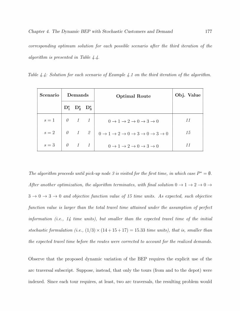
Chapter 4. The Dynamic BEP with Stochastic Customers and Demand 177
corresponding optimum solution for each possible scenario after the third iteration of the
algorithm is presented in Table 4.4.
Table 4.4: Solution for each scenario of Example 4.1 on the third iteration of the algorithm.
Scenario Demands Optimal Route Obj. Value
Ds1 Ds
2 Ds3
s = 1 0 1 1 0→ 1→ 2→ 0→ 3→ 0 11
s = 2 0 1 2 0→ 1→ 2→ 0→ 3→ 0→ 3→ 0 15
s = 3 0 1 1 0→ 1→ 2→ 0→ 3→ 0 11
The algorithm proceeds until pick-up node 3 is visited for the first time, in which case P ∗ = ∅.
After another optimization, the algorithm terminates, with final solution 0→ 1→ 2→ 0→
3 → 0 → 3 → 0 and objective function value of 15 time units. As expected, such objective
function value is larger than the total travel time attained under the assumption of perfect
information (i.e., 14 time units), but smaller than the expected travel time of the initial
stochastic formulation (i.e., (1/3)× (14 + 15 + 17) = 15.33 time units), that is, smaller than
the expected travel time before the routes were corrected to account for the realized demands.
Observe that the proposed dynamic variation of the BEP requires the explicit use of the
arc traversal subscript. Suppose, instead, that only the tours (from and to the depot) were
indexed. Since each tour requires, at least, two arc traversals, the resulting problem would
Chapter 4. The Dynamic BEP with Stochastic Customers and Demand 178
have considerably fewer variables and constraints, and, thus, improved tractability. However,
such approach may also lead to the construction of subtours within previously performed
routes. For instance, consider a network with three pick-up locations (nodes 1, 2, and 3) and
that a single bus is available for the evacuation. Now, suppose that, after two iterations of
the algorithm, the resulting route (saved into set R∗) is 0→ 1→ 2. At this point, the vehicle
is stationed at pick-up location 2, and only the demand at pick-up node 3 remains uncertain.
Logically, the vehicle may either be routed through arc (2, 3) or arc (2, 0). However, if only
the tours were indexed, then the model may choose to modify the previously performed
route to accommodate a visit to pick-up node 3 starting from pick-up node 1, that is, it may
choose to enforce the route 0→ 1→ 3→ 1→ 2, an impossibility.
The next section explores important properties of the proposed BEP variation, and leverages
these insights into an improved, deterministic formulation for the problem.
4.3 Problem Analysis
This Section explores important properties of the problem. It is shown that the proposed
stochastic formulation relies on exploratory visits (or sampling) to pick-up locations that
have not yet been visited in order to reduce the expected total travel time of the fleet, even
though, in some instances of the problem, such approach actually results in larger objective
function values. In addition, it is shown that, depending on the realized demand at the
destination nodes, symmetrical tours may not produce symmetrical results. These insights
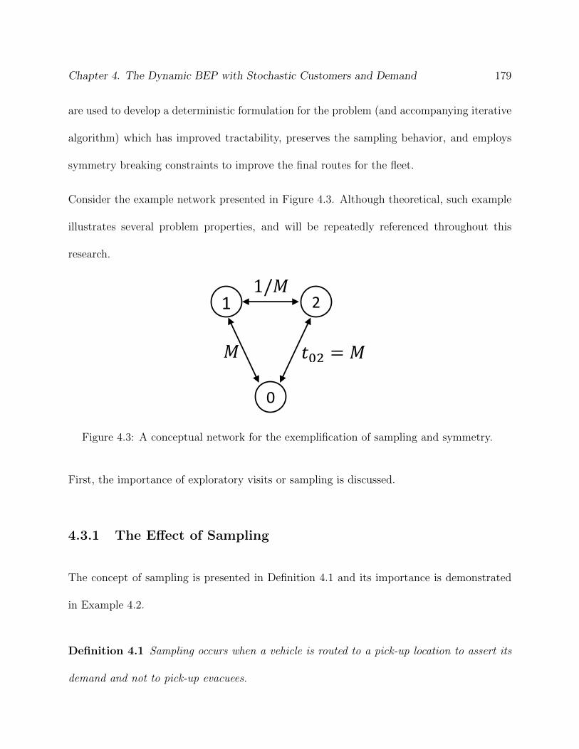
Chapter 4. The Dynamic BEP with Stochastic Customers and Demand 179
are used to develop a deterministic formulation for the problem (and accompanying iterative
algorithm) which has improved tractability, preserves the sampling behavior, and employs
symmetry breaking constraints to improve the final routes for the fleet.
Consider the example network presented in Figure 4.3. Although theoretical, such example
illustrates several problem properties, and will be repeatedly referenced throughout this
research.
2 1
0
Figure 4.3: A conceptual network for the exemplification of sampling and symmetry.
First, the importance of exploratory visits or sampling is discussed.
4.3.1 The Effect of Sampling
The concept of sampling is presented in Definition 4.1 and its importance is demonstrated
in Example 4.2.
Definition 4.1 Sampling occurs when a vehicle is routed to a pick-up location to assert its
demand and not to pick-up evacuees.
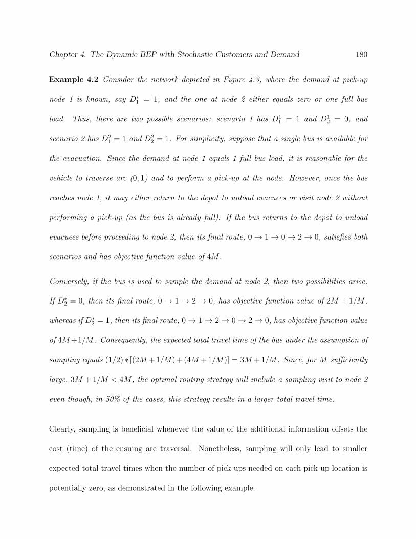
Chapter 4. The Dynamic BEP with Stochastic Customers and Demand 180
Example 4.2 Consider the network depicted in Figure 4.3, where the demand at pick-up
node 1 is known, say D∗1 = 1, and the one at node 2 either equals zero or one full bus
load. Thus, there are two possible scenarios: scenario 1 has D11 = 1 and D1
2 = 0, and
scenario 2 has D21 = 1 and D2
2 = 1. For simplicity, suppose that a single bus is available for
the evacuation. Since the demand at node 1 equals 1 full bus load, it is reasonable for the
vehicle to traverse arc (0, 1) and to perform a pick-up at the node. However, once the bus
reaches node 1, it may either return to the depot to unload evacuees or visit node 2 without
performing a pick-up (as the bus is already full). If the bus returns to the depot to unload
evacuees before proceeding to node 2, then its final route, 0→ 1→ 0→ 2→ 0, satisfies both
scenarios and has objective function value of 4M .
Conversely, if the bus is used to sample the demand at node 2, then two possibilities arise.
If D∗2 = 0, then its final route, 0→ 1→ 2→ 0, has objective function value of 2M + 1/M ,
whereas if D∗2 = 1, then its final route, 0→ 1→ 2→ 0→ 2→ 0, has objective function value
of 4M+1/M . Consequently, the expected total travel time of the bus under the assumption of
sampling equals (1/2)∗ [(2M + 1/M) + (4M + 1/M)] = 3M + 1/M . Since, for M sufficiently
large, 3M + 1/M < 4M , the optimal routing strategy will include a sampling visit to node 2
even though, in 50% of the cases, this strategy results in a larger total travel time.
Clearly, sampling is beneficial whenever the value of the additional information offsets the
cost (time) of the ensuing arc traversal. Nonetheless, sampling will only lead to smaller
expected total travel times when the number of pick-ups needed on each pick-up location is
potentially zero, as demonstrated in the following example.
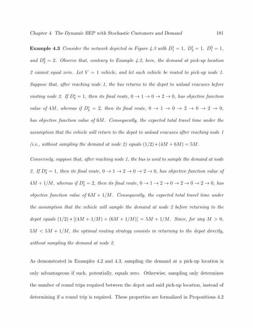
Chapter 4. The Dynamic BEP with Stochastic Customers and Demand 181
Example 4.3 Consider the network depicted in Figure 4.3 with D11 = 1, D1
2 = 1, D21 = 1,
and D22 = 2. Observe that, contrary to Example 4.2, here, the demand at pick-up location
2 cannot equal zero. Let V = 1 vehicle, and let such vehicle be routed to pick-up node 1.
Suppose that, after reaching node 1, the bus returns to the depot to unload evacuees before
visiting node 2. If D∗2 = 1, then its final route, 0→ 1→ 0→ 2→ 0, has objective function
value of 4M , whereas if D∗2 = 2, then its final route, 0 → 1 → 0 → 2 → 0 → 2 → 0,
has objective function value of 6M . Consequently, the expected total travel time under the
assumption that the vehicle will return to the depot to unload evacuees after reaching node 1
(i.e., without sampling the demand at node 2) equals (1/2) ∗ (4M + 6M) = 5M .
Conversely, suppose that, after reaching node 1, the bus is used to sample the demand at node
2. If D∗2 = 1, then its final route, 0→ 1→ 2→ 0→ 2→ 0, has objective function value of
4M + 1/M , whereas if D∗2 = 2, then its final route, 0→ 1→ 2→ 0→ 2→ 0→ 2→ 0, has
objective function value of 6M + 1/M . Consequently, the expected total travel time under
the assumption that the vehicle will sample the demand at node 2 before returning to the
depot equals (1/2) ∗ [(4M + 1/M) + (6M + 1/M)] = 5M + 1/M . Since, for any M > 0,
5M < 5M + 1/M , the optimal routing strategy consists in returning to the depot directly,
without sampling the demand at node 2.
As demonstrated in Examples 4.2 and 4.3, sampling the demand at a pick-up location is
only advantageous if such, potentially, equals zero. Otherwise, sampling only determines
the number of round trips required between the depot and said pick-up location, instead of
determining if a round trip is required. These properties are formalized in Propositions 4.2
Chapter 4. The Dynamic BEP with Stochastic Customers and Demand 182
and 4.3.
Proposition 4.2 If the demand at a given pick-up location is potentially zero, then a lower
expected total travel time may be attained by sampling the demand at this location.
Proof. See Example 4.2.
Proposition 4.3 If the demand at a given pick-up location is never zero, then a lower
expected total travel time cannot be attained by sampling the demand at this location.
Proof. See Example 4.3.
Next, the effect of symmetry is investigated.
4.3.2 The Effect of Symmetry
Here, the term symmetry refers to the problem default inability to distinguish between
seemingly identical first stage decisions (i.e., between subsequent arc traversals for each
vehicle leading to identical expected total travel times), but which may result in distinct
objective function values depending on the realized demands at the destination nodes. The
effect of symmetry is demonstrated in Example 4.4.
Example 4.4 Consider the network depicted in Figure 4.3 with D11 = 1, D1
2 = 0, D21 = 1,
and D22 = 1. Once again, suppose that a single bus is available for the evacuation, and
consider the ensuing symmetrical solutions presented in Table 4.5.
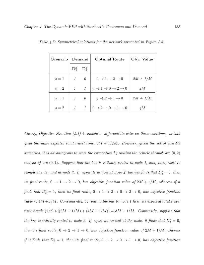
Chapter 4. The Dynamic BEP with Stochastic Customers and Demand 183
Table 4.5: Symmetrical solutions for the network presented in Figure 4.3.
Scenario Demand Optimal Route Obj. Value
Ds1 Ds
2
s = 1 1 0 0→ 1→ 2→ 0 2M + 1/M
s = 2 1 1 0→ 1→ 0→ 2→ 0 4M
s = 1 1 0 0→ 2→ 1→ 0 2M + 1/M
s = 2 1 1 0→ 2→ 0→ 1→ 0 4M
Clearly, Objective Function (4.1) is unable to differentiate between these solutions, as both
yield the same expected total travel time, 3M + 1/2M . However, given the set of possible
scenarios, it is advantageous to start the evacuation by routing the vehicle through arc (0, 2)
instead of arc (0, 1). Suppose that the bus is initially routed to node 1, and, then, used to
sample the demand at node 2. If, upon its arrival at node 2, the bus finds that D∗2 = 0, then
its final route, 0 → 1 → 2 → 0, has objective function value of 2M + 1/M , whereas if it
finds that D∗2 = 1, then its final route, 0 → 1 → 2 → 0 → 2 → 0, has objective function
value of 4M + 1/M . Consequently, by routing the bus to node 1 first, its expected total travel
time equals (1/2) ∗ [(2M + 1/M) + (4M + 1/M)] = 3M + 1/M . Conversely, suppose that
the bus is initially routed to node 2. If, upon its arrival at the node, it finds that D∗2 = 0,
then its final route, 0 → 2 → 1 → 0, has objective function value of 2M + 1/M , whereas
if it finds that D∗2 = 1, then its final route, 0 → 2 → 0 → 1 → 0, has objective function
Chapter 4. The Dynamic BEP with Stochastic Customers and Demand 184
value of 4M . Consequently, by routing the bus to node 2 first, its expected total travel time
equals (1/2) ∗ [(2M + 1/M) + (4M)] = 3M + 1/2M , a smaller value than the one attained
by routing the vehicle to pick-up node 1 first.
Interestingly, the difference between these symmetrical tours follows from an additional sam-
pling visit to pick-up node 2, which does not take place when arc (0, 2) is the first one
traversed. This property is formalized in Proposition 4.4.
Proposition 4.4 Even though the problem formulation assumes symmetrical arc traversal
times, symmetrical routes may not yield equal travel times. Better solutions may be attained
by prioritizing visits to pick-up locations that have, potentially, zero-demand.
Proof. See Example 4.4.
Next, an alternative, deterministic formulation that leverages these sampling and symmetry
properties is presented.
4.3.3 Deterministic Formulation
Recall that the first stage of the proposed two-stage stochastic formulation identifies the
subsequent arc traversal (common across scenarios) for each vehicle, whereas the second stage
identifies the remaining portion of their tour for each possible scenario realization. However,
since the problem is re-optimized as additional information becomes available, individual
outcomes of the second stage decision are redundant, and, thus, unnecessary. Consequently,
Chapter 4. The Dynamic BEP with Stochastic Customers and Demand 185
at least in a dynamic context, the previous two-stage stochastic formulation can be modified
to a deterministic equivalent, with arbitrary demands that are updated dynamically during
the course of the evacuation. Since scenarios are no longer explicitly modeled, the resulting
formulation has fewer variables and constraints, and, thus, is considerably more efficient.
However, such approach may prevent sampling from occurring, for, as shown in Examples
4.2 and 4.3 and formalized in Propositions 4.2 and 4.3, exploratory visits to pick-up locations
are only advantageous (and, thus, may only take place) when their demand is potentially
zero. Consequently, in order to preserve sampling, demands must be set to their lowest
realizable value (best-case scenario). Such concept is formalized in Proposition 4.5.
Proposition 4.5 Replacing the uncertain demands at each pick-up location with their worst-
case scenario reduces the problem size and the ensuing computation time. However, such
strategy also negates sampling, thus potentially leading to worse routing strategies.
Proof. Consider the network depicted in Figure 4.3 withD11 = 1, D1
2 = 0, D21 = 1, andD2
2 =
1. Once again, suppose that a single bus is available for the evacuation. Under the worst-
case strategy, D′2, the updated demand at node 2, is set to max{0, 1} = 1. Since the model
assumes that at least one pick-up is needed at node 2, there is no need to sample its actual
demand. Consequently, arc (1, 2) will never be traversed, even though, as demonstrated in
Example 4.2, such strategy reduces the expected total travel time of the fleet from 4M to
3M + 1/M , and, in 50% of the cases, leads to an actual solution as low as 2M + 1/M .
Such approach is counterintuitive, as it is common practice to assume the worst-case scenario

Chapter 4. The Dynamic BEP with Stochastic Customers and Demand 186
on each pick-up location in an attempt to improve the robustness of the problem, that is,
in an attempt to increase the likelihood that the chosen routes will satisfy any demand
realization. Here, however, setting the demands to their worst-case scenario on each pick-
up location merely leads to an upper bound on the overall travel time of the fleet, while
potentially worsening the final solution.
In summary, the deterministic formulation eliminates the scenario subscripts from the x and
y-variables and fixes the demands to their lowest realizable value on each pick-up location,
even if the resulting demands conflict with the set of possible scenarios (i.e., even if none
of the defined scenarios allow these demands to occur simultaneously). Moreover, the effect
of symmetry can be leveraged by preventing buses from leaving the depot towards pick-up
locations with uncertain, but positive, demand without a future return arc traversal from
such node. By prioritizing visits to pick-up locations that have, potentially, zero-demand,
such constraint breaks some of the problem symmetries in favor of arc traversals more likely
to reduce the total travel time of the fleet. Consequently, the deterministic formulation has
improved tractability, preserves the desired sampling behavior, and is able to break problem
symmetries in favor of arc traversals leading to improved final routes. Its decision variables,
objective function, and constraint set are as follows.

Chapter 4. The Dynamic BEP with Stochastic Customers and Demand 187
Table 4.6: Decision variables for the deterministic formulation.
Variable Description
xmtij binary variable that equals 1 if arc (i, j) is the tth arc traversed by vehicle m,
else 0, ∀ (i, j) ∈ A, m = 1, · · · , V, t = 1, · · · , T ;
ymtj percent capacity of vehicle m consumed at pick-up node j following its tth arc
traversal, ∀ j ∈ P, m = 1, · · · , V, t = 1, · · · , T . Let 0 ≤ ymtj ≤ 1, ∀ j ∈
P, m = 1, · · · , V, t = 1, · · · , T .
Proposed Deterministic Formulation:
Minimize∑
(i,j)∈A
V∑
m=1
T∑
t=1
tijxmtij (4.15)
Subject to
xm1ij = 0, ∀ i ∈ P, j : (i, j) ∈ A, m = 1, · · · , V (4.16)
∑
i:(i,j)∈A
xmtij =∑
k:(j,k)∈A
xm(t+1)jk , ∀ j ∈ P, m = 1, · · · , V, t = 1, · · · , T − 1 (4.17)
∑
i:(i,0)∈A
xmti0 ≥∑
k:(0,k)∈A
xm(t+1)0k , ∀ m = 1, · · · , V, t = 1, · · · , T − 1 (4.18)
xmTij = 0, ∀ j ∈ P, i : (i, j) ∈ A, m = 1, · · · , V (4.19)
∑
(i,j)∈A
xmtij ≤ 1, ∀ m = 1, · · · , V, t = 1, · · · , T (4.20)
Chapter 4. The Dynamic BEP with Stochastic Customers and Demand 188
ymtj ≤∑
i:(i,j)∈A
xmtij , ∀ j ∈ P, m = 1, · · · , V, t = 1, · · ·T (4.21)
∑
j∈P
t∑
l=1
ymlj −∑
i:(i,0)∈A
t∑
l=1
xmli0 ≤ 1, ∀ m = 1, · · · , V, t = 1, · · · , T (4.22)
V∑
m=1
T∑
t=1
ymtj = D′j, ∀ j ∈ P (4.23)
∑
i:(i,j)∈A
V∑
m=1
T∑
t=1
xmtij ≥ 1, ∀ j ∈ P ∗ (4.24)
D′j(T∑
l=t+1
xmlj0 − xmt0j ) ≥ 0, ∀ j ∈ P ∗, m = 1, · · · , V, t = 1, · · · , T − 1 (4.25)
xmtij = 1, ∀ {(i, j),m, t} ∈ R∗ (4.26)
ymtj = g, ∀ {j,m, t, g} ∈ C∗. (4.27)
Objective Function (4.15) minimizes the total travel time of the fleet under the best-case
scenario (i.e., the lowest possible demand realization) on each pick-up location. Constraints
(4.16)-(4.20) are similar to (4.2)-(4.6), preventing the construction of invalid routes, in-
cluding the elimination of subtours. Constraints (4.21)-(4.23) are similar to (4.7)-(4.9),
enforcing the vehicle capacity restrictions. Note that (4.23), contrary to (4.9), only en-
sures that the best-case demand, D′j, among the set of remaining scenarios, S∗, is met. Let
D′j = mins:(j,s)∈S∗ Dsj , ∀ j ∈ P ∗ and D′j = D∗j , ∀ j ∈ (P ∩ (P ∗)c). Constraint (4.10) is no
longer necessary, since every routing decision is now equal across scenarios. Constraint (4.24)
is similar to (4.11), but it is now defined only for pick-up locations with uncertain demand.
Since elements from S∗ are now iteratively removed, it may be possible to infer the demand
at some pick-up locations without an initial visit. Consequently, (4.24) allows pick-up lo-
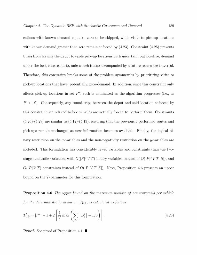
Chapter 4. The Dynamic BEP with Stochastic Customers and Demand 189
cations with known demand equal to zero to be skipped, while visits to pick-up locations
with known demand greater than zero remain enforced by (4.23). Constraint (4.25) prevents
buses from leaving the depot towards pick-up locations with uncertain, but positive, demand
under the best-case scenario, unless such is also accompanied by a future return arc traversal.
Therefore, this constraint breaks some of the problem symmetries by prioritizing visits to
pick-up locations that have, potentially, zero-demand. In addition, since this constraint only
affects pick-up locations in set P ∗, such is eliminated as the algorithm progresses (i.e., as
P ∗ 7→ ∅). Consequently, any round trips between the depot and said location enforced by
this constraint are relaxed before vehicles are actually forced to perform them. Constraints
(4.26)-(4.27) are similar to (4.12)-(4.13), ensuring that the previously performed routes and
pick-ups remain unchanged as new information becomes available. Finally, the logical bi-
nary restriction on the x-variables and the non-negativity restriction on the y-variables are
included. This formulation has considerably fewer variables and constraints than the two-
stage stochastic variation, with O(|P |2 V T ) binary variables instead of O(|P |2 V T |S|), and
O(|P |V T ) constraints instead of O(|P |V T |S|). Next, Proposition 4.6 presents an upper
bound on the T -parameter for this formulation:
Proposition 4.6 The upper bound on the maximum number of arc traversals per vehicle
for the deterministic formulation, T ′UB, is calculated as follows:
T ′UB = |P ∗|+ 1 + 2
⌈1
Vmax
(∑
j∈P
⌈D′j⌉− 1, 0
)⌉. (4.28)
Proof. See proof of Proposition 4.1.
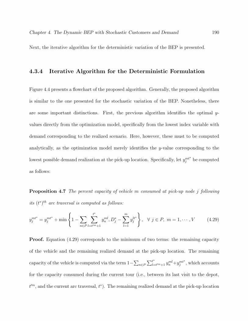
Chapter 4. The Dynamic BEP with Stochastic Customers and Demand 190
Next, the iterative algorithm for the deterministic variation of the BEP is presented.
4.3.4 Iterative Algorithm for the Deterministic Formulation
Figure 4.4 presents a flowchart of the proposed algorithm. Generally, the proposed algorithm
is similar to the one presented for the stochastic variation of the BEP. Nonetheless, there
are some important distinctions. First, the previous algorithm identifies the optimal y-
values directly from the optimization model, specifically from the lowest index variable with
demand corresponding to the realized scenario. Here, however, these must to be computed
analytically, as the optimization model merely identifies the y-value corresponding to the
lowest possible demand realization at the pick-up location. Specifically, let ymt∗
j be computed
as follows:
Proposition 4.7 The percent capacity of vehicle m consumed at pick-up node j following
its (t∗)th arc traversal is computed as follows:
ymt∗
j = ymt∗
j + min
{1−
∑
n∈P
t∗∑
l=t′m+1
ymln , D∗j −m∑
l=1
ylt∗
j
}, ∀ j ∈ P, m = 1, · · · , V (4.29)
Proof. Equation (4.29) corresponds to the minimum of two terms: the remaining capacity
of the vehicle and the remaining realized demand at the pick-up location. The remaining
capacity of the vehicle is computed via the term 1−∑n∈P∑t∗
l=t′m+1 ymln +ymt
∗j , which accounts
for the capacity consumed during the current tour (i.e., between its last visit to the depot,
t′m, and the current arc traversal, t∗). The remaining realized demand at the pick-up location

Chapter 4. The Dynamic BEP with Stochastic Customers and Demand 191
is computed via the term D∗j−∑m
l=1 ylt∗j +ymt
∗j , which accounts for any pick-ups by alternate,
lower index vehicles also visiting said location on their (t∗)th arc traversal. Observe that the
term ymt∗
j is part of both subtractions, and, thus, must be reinserted into the equation.
Second, the algorithm eliminates any scenarios that are no longer feasible from the problem
parameter set. Recall that such was not possible in the two-stage stochastic formulation, as
the decision variables were indexed for all elements in S. Third, since infeasible scenarios are
eliminated from the problem parameter set, D′j, the demand under the best-case scenario,
must be recomputed for the remaining elements in P ∗. Finally, any pick-up location with
a single realizable scenario is eliminated from P ∗, even if such location has not yet been
visited. Consequently, the algorithm allows pick-up locations with known zero-demand to
be skipped, while still ensuring that every evacuee boards a transit vehicle.
In summary, the algorithm proceeds as follows. First, the parameters t∗, C∗, R∗, and P ∗ are
initialized. Recall that t∗ corresponds to the current iteration of the algorithm, and, thus,
to the subsequent arc traversal of each vehicle; that C∗ corresponds to the set of previously
performed pick-ups; that R∗ corresponds to the set of previously traversed arcs; and that
P ∗ corresponds to the set of pick-up locations with uncertain demand. Observe that the
parameter P ∗ is now part of the proposed formulation. In addition, let t′m, m = 1, · · · , V ,
denote the last arc traversal in which the mth vehicle visited the depot, and let z1, z2, and
T ′ be support parameters. On each iteration of the proposed algorithm, the T -parameter
is updated. Since the algorithm eliminates non-realizable scenarios from the set of possible
demand realizations, it may avoid visiting pick-up locations which have known demand
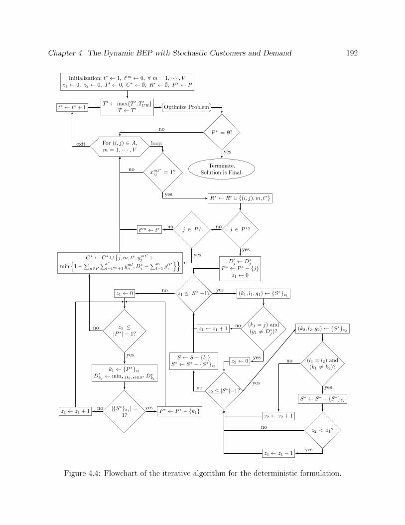
Chapter 4. The Dynamic BEP with Stochastic Customers and Demand 192
Initialization: t∗ ← 1, t′m ← 0, ∀ m = 1, · · · , Vz1 ← 0, z2 ← 0, T ′ ← 0, C∗ ← ∅, R∗ ← ∅, P ∗ ← P
T ′ ← max{T ′, T ′UB}T ← T ′
Optimize Problemt∗ ← t∗ + 1
For (i, j) ∈ A,m = 1, · · · , V
xmt∗ij = 1?
R∗ ← R∗ ∪ {(i, j),m, t∗}
j ∈ P ∗?j ∈ P?t′m ← t∗
C∗ ← C∗ ∪{j,m, t∗, ymt∗
j +
min{1−∑n∈P
∑t∗
l=t′m+1 ymln , D∗j −
∑ml=1 y
lt∗j
}} D′j ← D∗jP ∗ ← P ∗ − {j}
z1 ← 0
z1 ≤ |S∗|−1? (k1, l1, g1)← {S∗}z1
(k1 = j) and(g1 6= D∗j )?
z1 ← z1 + 1
S ← S − {l1}S∗ ← S∗ − {S∗}z1
z2 ← 0
z2 ≤ |S∗|−1?
(k2, l2, g2)← {S∗}z2
(l1 = l2) and(k1 6= k2)?
S∗ ← S∗ − {S∗}z2
z2 ← z2 + 1
z2 < z1?
z1 ← z1 − 1
z1 ← 0
z1 ≤|P ∗| − 1?
k1 ← {P ∗}z1D′k1← mins:(k1,s)∈S∗ D
sk1
|{S∗}z1 | =1?
z1 ← z1 + 1 P ∗ ← P ∗ − {k1}
P ∗ = ∅?
Terminate.Solution is Final.
loopexit
no
yes
no
yes
nono
yes
yes
no
yes
no
yes
no
no yes
yesno
no
no
yes
yes
yes
Figure 4.4: Flowchart of the iterative algorithm for the deterministic formulation.

Chapter 4. The Dynamic BEP with Stochastic Customers and Demand 193
equal to zero. Consequently, T ′UB may not change monotonically with t∗. In order to prevent
conflicts with previously added elements in R∗ and C∗, the monotonically increasing behavior
of T is enforced via the support parameter T ′. The problem is reoptimized; the (t∗)th arc
traversal of each vehicle, if any, is saved into set R∗; and its percent capacity occupied at
the destination node (if such is a pick-up location) is saved into set C∗. Observe that the
realized y-value is now computed via (4.29). If the destination node is a pick-up location
that has not yet been visited, then such is removed from set P ∗ and its demand set to D∗j .
In addition, any infeasible scenarios are removed from set S∗ and the lowest demand among
the remaining scenarios, D′j, is recomputed for each pick-up node j ∈ P ∗. Conversely, if
the destination node is the depot, then the corresponding t′m parameter is set to t∗. The
algorithm terminates once P ∗ = ∅, in which case the solution attained by the optimization
problem is final. Otherwise, t∗ is incremented by one and a new iteration is performed.
Example 4.5 shows the implementation of the algorithm for the same theoretical network
used to exemplify the first algorithm.
Example 4.5 Once again, consider the example network presented in Figure 4.2 with V = 1
bus. Provided the scenarios presented in Table 4.2, the lowest realizable demand on each pick-
up location equals D′1 = 0, D′2 = 1, and D′3 = 1. Since D′2, D′3 > 0 and since V = 1, by
(4.25), x1t0j ≤
∑Tl=t+1 x
1lj0, ∀ j ∈ {2, 3}, t = 1, · · · , T − 1, forcing any traversals through
arcs (0, 2) and (0, 3) to be followed by at least one future traversal through arcs (2, 0) and
(3, 0), respectively. Since such round trips do not reduce the expected total travel time of the
fleet, arc (0, 1) is preferred. While the same arc was initially traversed in Example 4.1, it

Chapter 4. The Dynamic BEP with Stochastic Customers and Demand 194
is important to observe that such occurred merely by chance, as, for example, the algorithm
was unable to distinguish between the tours 0 → 1 → 2 → 0 and 0 → 2 → 1 → 0. Here,
however, this symmetry is broken in favor of arc traversals leading to pick-up locations with,
potentially, zero demand (i.e., node 1).
Now, suppose that the realized demand at node 1, once again, equals zero (i.e., suppose that
D∗1 = 0). Since the demand at this location is now known, the location is removed from set
P ∗. In addition, sets R∗ and C∗ are updated to reflect the realized arc traversal and pick-up,
respectively, that is, R∗set= {{(0, 1), 1, 1}} and C∗
set= {{1, 1, 1, 0}}; and scenario 1 is removed
from the problem parameter set. Such change, however, does not affect the best-case scenario
demands for the remaining nodes in P ∗. Finally, t∗ is incremented by one, and the problem
is reoptimized.
As in Example 4.1, the bus is directed to pick-up node 2. Now, suppose that the realized
demand at node 2 equals one full bus load (i.e., suppose that D∗2 = 1). In this case,
R∗set= {{(0, 1), 1, 1}, {(1, 2), 1, 2}}, C∗ set
= {{1, 1, 1, 0}, {2, 1, 2, 1}}, and P ∗set= {3}. How-
ever, provided this demand realization, scenario 3 cannot take place, and is removed from
S∗. Consequently, the only realizable demand at pick-up node 3 is D∗3 = 2. Since the demand
at this location is now known, the location is removed from set P ∗, t∗ is incremented by one,
and the problem is reoptimized. Since P ∗ is now empty, the algorithm terminates, with final
solution 0 → 1 → 2 → 0 → 3 → 0 → 3 → 0 and objective function value of 15 time units.
Observe that, here, the final solution was attained in two iterations, whereas, previously, four
iterations were needed.

Chapter 4. The Dynamic BEP with Stochastic Customers and Demand 195
Interestingly, since the problem starts with the premise of the best-case scenario on each
pick-up location and since additional arc traversals are iteratively added to accommodate the
realized demand in excess of the original assumption, the objective function value attained
by the algorithm increases monotonically with t∗. Consequently, this algorithm starts from
a possibly infeasible route and iteratively adds arc traversals to it until the realized demand
on every pick-up location is accommodated. Conversely, the previous algorithm starts from
a set of feasible routes, one for each scenario, and modify them (possibly leading some of
these to infeasibility during intermediary iterations), until they all converge to a single route
that meets the realized demand on each pick-up location. The next Section compares these
formulations and accompanying algorithms in terms of tractability and solution quality.
4.3.5 Algorithm Comparison
As indicated by Pillac et al. (2013), improving the solution time of the model is particularly
important in D-VRPs given the potentially large frequency of requests and the urgency of
the requests. The same premise holds true for dynamic variations of the BEP, as buses
must remain parked at the pick-up locations waiting for further instructions. This section
empirically explores the performance of both formulations and related algorithms for solving
a somewhat larger problem instance. All computational runs were performed using IBM
ILOG CPLEX Optimization Studio version 12.4 on a PC with two quad-core, 2.13 GHz
Intel Xeon processors and 4.00 GB RAM running on a 64-Bit operating system.

Chapter 4. The Dynamic BEP with Stochastic Customers and Demand 196
Consider the example network depicted in Figure 4.5 with five pick-up locations scattered
around an evacuation zone, possibly the vicinity of a building under bomb threat. The prob-
lem requires every evacuee to be transported to a depot/shelter, but their exact number, if
any, is only revealed after an initial visit by a vehicle. The set of possible demand realizations
is presented in Table 4.7.
0
3 2
1
4
16
5
15
19
14
17
3 3
3
3
3
5
5 5
5 5
Figure 4.5: An example network for the algorithm comparison.
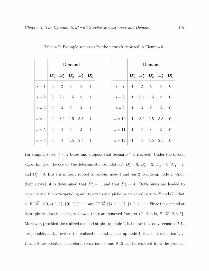
Chapter 4. The Dynamic BEP with Stochastic Customers and Demand 197
Table 4.7: Example scenarios for the network depicted in Figure 4.5.
Demand Demand
Ds1 Ds
2 Ds3 Ds
4 Ds5 Ds
1 Ds2 Ds
3 Ds4 Ds
5
s = 1 0 2 0 4 1 s = 7 1 2 0 4 0
s = 2 0 2.5 1.5 4 1 s = 8 1 2.5 1.5 4 0
s = 3 0 3 0 3 1 s = 9 1 3 0 3 0
s = 4 0 3.2 1.5 3.3 1 s = 10 1 3.2 1.5 3.3 0
s = 5 0 4 0 2 1 s = 11 1 4 0 2 0
s = 6 0 4 1.5 2.5 1 s = 12 1 4 1.5 2.5 0
For simplicity, let V = 2 buses and suppose that Scenario 7 is realized. Under the second
algorithm (i.e., the one for the deterministic formulation), D′1 = 0, D′2 = 2, D′3 = 0, D′4 = 2,
and D′5 = 0. Bus 1 is initially routed to pick-up node 4 and bus 2 to pick-up node 1. Upon
their arrival, it is determined that D∗1 = 1 and that D∗4 = 4. Both buses are loaded to
capacity and the corresponding arc traversals and pick-ups are saved to sets R∗ and C∗, that
is, R∗set= {{(0, 4), 1, 1}, {(0, 1), 2, 1}} and C∗
set= {{4, 1, 1, 1}, {1, 2, 1, 1}}. Since the demand at
these pick-up locations is now known, these are removed from set P ∗, that is, P ∗set= {2, 3, 5}.
Moreover, provided the realized demand at pick-up node 1, it is clear that only scenarios 7-12
are possible, and, provided the realized demand at pick-up node 4, that only scenarios 1, 2,
7, and 8 are possible. Therefore, scenarios 1-6 and 9-12 can be removed from the problem
Chapter 4. The Dynamic BEP with Stochastic Customers and Demand 198
parameter set, D′1set= 1, and D′4
set= 4. The remaining problem parameters, other than t∗,
remain unchanged. On the second iteration, the first bus is routed to the depot to unload
evacuees and the second bus is used to sample the realized demand at pick-up node 3. Upon
its arrival, it is determined that D∗3 = 0. Consequently, scenario 8 is no longer possible,
and is removed from the problem parameter set. The D′j demands are set to the demand
realizations of scenario 7, R∗set= {{(0, 4), 1, 1}, {(0, 1), 2, 1}, {(4, 0), 1, 2}, {(1, 3), 2, 2}}, C∗ set=
{{4, 1, 1, 1}, {1, 2, 1, 1}, {3, 2, 2, 0}}, t∗ is incremented by one, and the problem is reoptimized.
Since P ∗ is now empty, the algorithm terminates. Under the final solution, bus 1 is routed
though arcs 0 → 4 → 0 → 4 → 0 → 4 → 0, transporting three full bus loads from pick-up
node 4 to the depot, and bus 2 is routed through arcs 0 → 1 → 3 → 0 → 2 → 0 → 4 →
0 → 2 → 0, transporting a full bus load from pick-up nodes 1 and 4 and two full bus loads
from pick-up node 2 to the depot. Under this routing strategy, the realized total travel time
equals 210 time units. Note that pick-up node 5 was never visited, as the algorithm correctly
inferred that its realized demand equals zero.
Both algorithms have worst-case complexity of polynomial order: the first algorithm has
O(|P |4 V |S|), whereas the second has O(|P |5 V |S|2). While more cumbersome, the second
algorithm is much more efficient, as it allows the use of a considerably smaller problem
formulation, an important consideration since even small variations of the classic VRP are
known to be NP-Hard (Toth and Vigo, 2002). In fact, the first iteration of the second
algorithm required 9.9 seconds, the second 4.6 seconds, and the last optimization 2.6 seconds.
A solution for the first algorithm could not be obtained, as it exceeded the computer memory
Chapter 4. The Dynamic BEP with Stochastic Customers and Demand 199
capacity on its very first iteration, after 12 hours and 33 minutes of computation and with
an optimality gap of 18.11%.
Alternative empirical experiments attained similar results. Consider an instance of the
example network depicted in Figure 4.5, with V = 2 buses, and involving only 3 sce-
narios: the first scenario has demands D11 = 0, D1
2 = 2, D13 = 0.5, D1
4 = 1.5, and
D15 = 1; the second, D2
1 = 0, D22 = 2, D2
3 = 0, D24 = 2, and D2
5 = 1; and the third,
D31 = 1, D3
2 = 1.5, D33 = 0.5, D3
4 = 2, and D35 = 0. Suppose that scenario 1 is realized. The
second algorithm was able to attain the final solution in one iteration, under 3.6 seconds,
and an additional 2.6 seconds for the last optimization. Conversely, the first algorithm re-
quired 5 iterations, with 102 hours and 19 minutes for the first iteration, 4 minutes and 34
seconds for the second, 36 seconds for the third, 2 seconds for the fourth, 1.5 seconds for
the fifth, and an additional second for the last optimization. Final objective function values
also differed, with 157 for the first algorithm and 155 for the second, which, interestingly,
is the optimum solution for the problem under the assumption of perfect information. The
next section summarizes the main findings of this paper and presents directions for future
research.
4.4 Conclusion and Future Research
This research introduced a two-stage stochastic formulation and an iterative algorithm for
solving a variation of the BEP in which the realized demands on each pick-up location are

Chapter 4. The Dynamic BEP with Stochastic Customers and Demand 200
only revealed during the course of the evacuation. The effect of sampling and symmetry
over the expected total travel time of the fleet is explored, and these insights leveraged
into an alternative, deterministic formulation. Such formulation has considerably improved
tractability, preserves the desired sampling behavior, and employs constraints that break
some of the problem symmetries in favor of arc traversals leading to reduced total travel
times. Despite such advances, both variations rely on simplifying assumptions that diminish
their usefulness to practitioners. First, they do not account for the time-dependent arrival
behavior of evacuees, and, instead, assume that these are at the pick-up locations at the
onset of the evacuation. While such assumption is realistic for no-notice evacuation settings
(such as the evacuation of urban clusters facing bomb threats), it fails to consider situations
in which enough time is available for adequate planning and implementation (such as a
region-wide evacuation preceding the arrival of a hurricane). Second, they neither limit
nor attempt to minimize the duration of the evacuation. While it is relatively easy to
incorporate any measure of completion time into the proposed formulations, further research
is needed to determine if the properties of sampling and symmetry (and, thus, the alternative
deterministic formulation) remain valid. Third, they do not balance the benefits of holding
buses at the depot or at the pick-up locations until other vehicles have reached their respective
destinations. By eliminating unnecessary visits to pick-up locations, such delay may reduce
the expected total travel time of the fleet, and, perhaps, the duration of the evacuation.
Fourth, the assumption that all scenarios have equally likely probability of realization is
unrealistic for most real-world evacuation settings. As shown by Fajardo and Waller (2012),
Chapter 4. The Dynamic BEP with Stochastic Customers and Demand 201
it is possible to derive the probabilities of each scenario realization directly from a Markov
Chain, at least in a D-TSP context. Nonetheless, even if such probabilities were available,
it is likely that the realized demands at the pick-up locations would fail to match any of the
predetermined scenarios. Further research is needed to accommodate fuzzy variations of the
problem, capable of adjusting the demand (and the likelihood) of the remaining scenarios as
new information becomes available.
Chapter 5
Conclusions
202

Chapter 5. Conclusions 203
This dissertation introduces and analyzes important variations of the Bus Evacuation Prob-
lem, a unique VRP motivated both by its humanitarian significance and by the routing and
scheduling challenges of planning transit-based, regional evacuations. Although this research
focuses on evacuation planning and implementation, the concepts herein developed are read-
ily applicable to many other transportation settings, within and outside the humanitarian
logistics ambit.
Chapter 2 presents and examines several structural properties of a particularly complex
variant of the BEP. The problem assumes that evacuees gather at the pick-up locations at
constant rates, from the start of the evacuation to a location-specific end-time (dictated by
risk considerations), and seeks a pick-up schedule at these locations, and the corresponding
routes for a fleet of buses, in such a way that their total waiting time (exposure) is mini-
mized. At each scheduled pick-up time, all evacuees present must be served and eventually
transported to a depot/shelter. The formulation forces at least one pick-up to take place
at each pick-up location, scheduled for the time when the arrival process of evacuees ends.
Efficiencies from allowing buses to unload evacuees at the depot multiple times and from
service choice, that is, from allowing the model to select the optimal number of pick-ups at
each location (up to a maximum service level), are exploited. It is shown that, under certain
conditions, if a feasible solution does not exist, then one can be obtained by increasing the
fleet size; that if one exists, then the exposure can be reduced by either increasing the fleet
size or the maximum service level; and that, after the minimum exposure schedule for a given
service level is attained, the exposure can only be reduced by further increasing the maxi-
Chapter 5. Conclusions 204
mum service level, but with diminishing returns. In addition, upper and lower bounds on the
fleet size required for feasibility and for such bound on exposure, and an exact formulation
and an upper bound on the maximum number of arc traversals per vehicle, were proposed.
More importantly, it is shown that, depending on the problem instance, it is possible to
reduce both the fleet size requirement and the amount of time that evacuees must wait for
rescue, and that, past a certain threshold, there is an optimal choice for the maximum service
level (or a range of potential values, if the problem cannot be solved to optimality under
a reasonable amount of time) that guarantees an efficient usage of the available fleet and
equitable reductions in exposure across pick-up locations. Appendix B presents alternative
formulations for such BEP variant.
Chapter 3 introduces an exact optimization algorithm based on a less known relaxation
methodology originally developed by Ritter (1967). The algorithm was selected due to its
ability to explore the inherent structure of problems with both complicating variables and
constraints, such as the aforementioned BEP variant, without the need to compound multiple
decomposition/relaxation strategies. In summary, the algorithm relaxes some of the non-
negativity and integer restrictions in order to produce a smaller and easier to solve problem,
namely the Reduced Problem. In the original algorithm, the relaxed non-negativity restric-
tions are enforced sequentially either by swapping decision variables between the relaxed
and non-relaxed sets (and recomputing the Reduced Problem parameters) or by adding new
constraints to the Reduced Problem. The algorithm terminates once the optimum solution
to the Reduced Problem also satisfies the non-negativity restriction of all relaxed variables.
Chapter 5. Conclusions 205
The proposed variation is similar to the original algorithm, except that it precludes swap-
ping of decision variables between the relaxed and non-relaxed sets. Hence, the modified
algorithm relies solely on the inclusion of constraints into the Reduced Problem in order to
enforce the non-negativity (and, now, the integer restriction) of the relaxed variables. By
preventing the swapping operation from taking place, the modified algorithm requires fewer
matrix manipulations and fewer numerical comparisons, and, thus, has improved numerical
stability. Perhaps even more important, given the dichotomous nature of the added con-
straints, the modified algorithm can be combined with the branch and bound algorithm in
order to allow problems with integer or mixed-integer subproblems to be solved to optimality.
Appendix C presents an example problem which is solved algebraically via the original and
modified algorithms. Such example problem is then modified to an integer, mixed-integer,
and, later, mixed-integer with a quadratic objective function variation and resolved using
the modified algorithm. Appendix D presents the MathWorks Matlab source code for the
original and modified algorithms. Empirical studies demonstrate its viability to solve large,
bordered-structure, optimization problems.
Finally, Chapter 4 introduces a two-stage stochastic formulation and an iterative (dynamic)
algorithm for the Bus Evacuation Problem. In this problem, a fleet of capacitated buses must
transport all transit-dependent individuals from a set of pick-up locations to a depot/shelter
with minimum total travel time. The problem assumes that a set of equal-probability demand
scenarios is available, and that the exact number of evacuees on each location, if any, becomes
known once a bus visits it for the first time. The effect of exploratory visits (sampling) and
Chapter 5. Conclusions 206
symmetry is explored, and the resulting insights used to develop a deterministic formulation
for the problem. While, at least in a dynamic context, these formulations are equivalent, the
deterministic variation has considerably improved tractability, preserves the desired sampling
behavior, and employs constraints that break some of the problem symmetries in favor of
arc traversals leading to reduced total travel times. Appendix E presents the IBM ILOG
CPLEX source code for solving both the two-stage and the deterministic formulations.
Despite these advances, the modeling and optimization literature on bus-based evacuation
planning and implementation is scarce and considerable research remains needed. First, the
variant presented in Chapter 2 assumes that evacuees arrive at the pick-up locations at a
constant rate. While such is an important distinction from the related literature, it is still
unrealistically portraying the true evacuee arrival behavior, which is probabilistic in nature
and is likely to vary over time. Conversely, while the problem variant presented in Chapter
4 assumes stochastic demand, it relies on simplifying assumptions that diminish its resem-
blance to real-life evacuation settings. First, the formulations presented in this Chapter
do not account for the time-dependent arrival behavior of evacuees, as the ones presented
in Chapter 2 and Appendix B. Instead, they assume that all evacuees are at the pick-up
locations upon the start of the evacuation. While such assumption is realistic for modeling
no-notice evacuation problems, such as the evacuation of urban clusters facing bomb threats,
it fails to consider situations in which enough time is available for its adequate planning and
implementation, such as a region-wide evacuation preceding the arrival of a hurricane. Sec-
ond, the formulations presented in Chapter 4 neither attempt to minimize the duration of

Chapter 5. Conclusions 207
the evacuation nor limit its completion time. While it is relatively easy to incorporate some
measure of completion time into the proposed formulations, further research is needed to de-
termine if the properties of sampling and symmetry (and, thus, the alternative deterministic
formulation proposed) remain valid. Third, these formulations do not balance the benefits
of holding buses at the depot or at the pick-up locations until other vehicles have reached
their respective destinations. By waiting for the demand at these locations to unravel, un-
necessary sampling visits may be avoided, thus leading to a reduction in the expected total
travel time of the fleet, and, perhaps, in the duration of the evacuation. In addition, while
it is common practice to use a scenario-based approach to model stochastic problems, the
assumption that these have equally likely probability of realization is unrealistic. Varying
probabilities can be attained from a Markov Chain (provided that the stochastic process is
memoryless and follows a known probability distribution) and incorporated into the model
via weight coefficients for the objective function. Nonetheless, in most real-world evacuation
settings, it is unlikely that the realized demands at the pick-up locations would match any of
the predetermined scenarios. Further research is needed to accommodate fuzzy variations of
the problem, capable of adjusting the demand (and the likelihood) of the remaining scenarios
as new information becomes available.
In addition, it remains computationally expensive to obtain an optimal solution to the BEP
variant presented in Chapter 2. Currently, the problem can only be solved to optimality for
toy examples involving few buses, pick-ups, and pick-up locations. As aforementioned, the
Modified Ritter (1967) Relaxation Algorithm presented in Chapter 3 is a general purpose
Chapter 5. Conclusions 208
algorithm, capable of solving bordered-structure problems with linear, integer, or mixed-
integer subproblems and with linear or quadratic objective functions. However, further
research is needed to determine the algorithm viability to solve such a BEP variant. In
particular, it may be possible to leverage inheriting structural properties of the problem into
the solution algorithm. First, the existence of non-singular matrices on each subproblem (i.e.,
within the constraint set coordinating the tour for each vehicle) would eliminate the need to
augment the original problem with artificial variables, and, thus, unnecessary computations.
Second, it may be advantageous to set the relaxed decision variables to the tours leading to
the minimum exposure schedule for a given service level. As shown in Chapter 2, such a pick-
up schedule, albeit sometimes infeasible, presents a lower bound on the objective function
value, and, thus, may expedite the fathoming of unprofitable branches during the branch and
bound algorithm. Finally, since the complicating constraints are equalities, they can be used
to eliminate the complicating variables from the original problem by simple substitution. As
a result, the inheriting bordered-structure of the problem would change to a block diagonal
or angular structure (as demonstrated in Appendix B), where the subproblem structure
(i.e., the decision variables and constraints controlling the routing, scheduling, and loading
restrictions for a vehicle) remain unchanged, and the complicating constraints change to
the allocation of evacuees to individual vehicles. Although such formulation has a simpler
structure, empirical studies have demonstrated that the ensuing increase in the number
of non-zero coefficients (problem density) leads to an increase in solution time when no
decomposition/relaxation strategy is used. Nonetheless, such formulation allows the problem
Chapter 5. Conclusions 209
to be solved by Dantzig-Wolfe Decomposition (Dantzig and Wolfe, 1960), or, in turn, its
dual problem solved by Benders’ Decomposition (Benders, 1962). Research is needed to
determine whether such algorithms, when used to solve such a dual angular formulation
of the aforementioned BEP variant, are able to attain faster computation times than the
Modified Ritter (1967) Relaxation Algorithm applied the original formulation.
Finally, considerable research is needed to improve the Modified Ritter (1967) Relaxation
Algorithm itself. As indicated in Chapter 3, the same concerns pertaining to the branch and
bound algorithm, namely as branching strategy and choice of branching variable, also apply
to the proposed algorithm. Consequently, further development of the source code presented
in Appendix D.2 is needed before the algorithm is able to systematically outperform com-
mercial optimization packages such as IBM ILOG CPLEX. In addition, since a considerable
amount of computational effort is dedicated to the generation of constraints enforcing the
branching and the upper and lower bound restrictions, and since these are incorporated se-
quentially into the Reduced Problem, it may be possible to further improve the efficiency
of the algorithm by the concomitant use of Gomory cuts. Finally, since the algorithm is
designed for bordered-structure problems, it may be applicable to seemingly structureless
problems, but which can be mapped into an structured problem through rearrangement of
their constraint coefficients. See Aykanat et al. (2004), Duff and Scott (2005), Ferris and
Horn (1998), Fragniere et al. (2000), Pinar and Aykanat (1996), and Pinar et al. (1996) for
multiple algorithms to reorganize the coefficients of the constraint matrix into exploitable
structures.
References
210
Aarts, E., Korst, J., and Laarhoven, P. V. (1997). Simulated annealing. In Aarts, E.
and Lenstra, J., editors, Local Search in Combinatorial Optimization, pages 91–120. John
Wiley & Sons Ltd.
Abdelgawad, H. and Abdulhai, B. (2010). Managing large-scale multimodal emergency
evacuations. Journal of Transportation Safety & Security, 2(2):122–151.
Abdelgawad, H., Abdulhai, B., and Wahba, M. (2010a). Multiobjective optimization for
multimodal evacuation. Transportation Research Record: Journal of the Transportation
Research Board, 2196(1):21–33.
Abdelgawad, H., Abdulhai, B., and Wahba, M. (2010b). Optimizing mass transit utilization
in emergency evacuation of congested urban areas. In Proceedings of the 89th Annual
Meeting of the Transportation Research Board, Washington, DC. Transportation Research
Board of the National Academies.
Angel, R., Caudle, W., Noonan, R., and Whinston, A. (1972). Computer-assisted school bus
scheduling. Management Science, 18(6):B279–B288.
Archetti, C. and Speranza, M. (2012). Vehicle routing problems with split deliveries. Inter-
national Transactions in Operational Research, 19(1-2):3–22.
211

References 212
Aykanat, C., Pinar, A., and Catalyurek, U. (2004). Permuting sparse rectangular matrices
into block-diagonal form. SIAM Journal on Scientific Computing, 25(6):1860–1879.
Balinski, M. and Quandt, R. (1964). On an integer program for a delivery problem. Opera-
tions Research, 12(2):300–304.
Basu, S. and Ghosh, D. (2008). A review of the tabu search literature on traveling salesman
problems. Indian Institute of Management, Ahmedabad, India.
Bazaraa, M., Jarvis, J., and Sherali, H. (2005). Linear programming and network flows.
Wiley Interscience, Hoboken, NJ, 3rd edition.
Bazaraa, M., Sherali, H., and Shetty, C. (2006). Nonlinear programming: theory and algo-
rithms. Wiley Interscience, Hoboken, NJ, 3rd edition.
Bell, J. and McMullen, P. (2004). Ant colony optimization techniques for the vehicle routing
problem. Advanced Engineering Informatics, 18(1):41–48.
Benders, J. (1962). Partitioning procedures for solving mixed-variables programming prob-
lems. Numerische Mathematik, 4(1):238–252.
Bish, D. (2011). Planning for a bus-based evacuation. OR Spectrum, 33(3):629–654.
Brooks, S. and Morgan, B. (1995). Optimization using simulated annealing. Journal of the
Royal Statistical Society. Series D (The Statistician), 44(2):241–257.
Brotcorne, L., Laporte, G., and Semet, F. (2003). Ambulance location and relocation models.
European Journal of Operational Research, 147(3):451–463.
References 213
Charnes, A. and Cooper, W. (1963). Deterministic equivalents for optimizing and satisficing
under chance constraints. Operations Research, 11(1):18–39.
Chen, C. and Chou, C. (2009). Modeling and performance assessment of a transit-based
evacuation plan within a contraflow simulation environment. Transportation Research
Record: Journal of the Transportation Research Board, 2091(1):40–50.
Christofides, N. and Beasley, J. (1984). The period routing problem. Networks, 14(2):237–
256.
Christofides, N., Mingozzi, A., and Toth, P. (1981). Exact algorithms for the vehicle routing
problem, based on spanning tree and shortest path relaxations. Mathematical Program-
ming, 20(1):255–282.
Clarke, G. and Wright, J. (1964). Scheduling of vehicles from a central depot to a number
of delivery points. Operations Research, 12(4):568–581.
Colorni, A., Dorigo, M., and Maniezzo, V. (1991). Distributed optimization by ant colonies.
In Varela, F. and Bourgine, P., editors, Proceedings of the 1st European Conference on
Artificial Life (ECAL’91), volume 142, pages 134–142, Paris, France. Elsevier Publishing.
Cordeau, J. and Laporte, G. (2003). The Dial-a-Ride problem (DARP): Variants, modeling
issues and algorithms. 4OR, 1(2):89–101.
Cordeau, J. and Laporte, G. (2006). Modeling and optimization of vehicle routing and arc
routing problems. In Gautam, M., Pitsoulis, L., and Williams, H., editors, Handbook

References 214
on Modelling for Discrete Optimization, volume 88 of International Series in Operations
Research & Management Science, pages 151–191. Springer US.
Dantzig, G., Fulkerson, R., and Johnson, S. (1954). Solution of a large-scale traveling-
salesman problem. Journal of the Operations Research Society of America, 2(4):393–410.
Dantzig, G. and Ramser, J. (1959). The truck dispatching problem. Management Science,
6(1):80–91.
Dantzig, G. and Wolfe, P. (1960). Decomposition principle for linear programs. Operations
Research, 8(1):101–111.
Deai, C., Wangtu, X., and Wei, Z. (2011). Optimize the transit vehicle routing for the
emergency evacuation. Advanced Materials Research, 201-203:1075–1081.
Delgado, F., Munoz, J., Giesen, R., and Cipriano, A. (2009). Real-time control of buses in
a transit corridor based on vehicle holding and boarding limits. Transportation Research
Record: Journal of the Transportation Research Board, 2090(1):59–67.
Duff, I. and Scott, J. (2005). Stabilized bordered block diagonal forms for parallel sparse
solvers. Parallel Computing, 31(3):275–289.
Eksioglu, B., Vural, A. V., and Reisman, A. (2009). The vehicle routing problem: A taxo-
nomic review. Computers & Industrial Engineering, 57(4):1472–1483.
Fajardo, D. and Waller, S. (2012). Dynamic traveling salesman problem in stochastic-state
References 215
network setting for search-and-rescue application. Transportation Research Record: Jour-
nal of the Transportation Research Board, 2283(1):122–130.
Ferris, M. and Horn, J. (1998). Partitioning mathematical programs for parallel solution.
Mathematical Programming, 80(1):35–61.
Fragniere, E., Gondzio, J., Sarkissian, R., and Vial, J. (2000). A structure-exploiting tool in
algebraic modeling languages. Management Science, 46(8):1145–1158.
Francis, P., Smilowitz, K., and Tzur, M. (2006). The period vehicle routing problem with
service choice. Transportation Science, 40(4):439–454.
Friedrich, C. (2006). The periodical vehicle routing problem: research overview and practical
application to a south German fast food restaurant. PhD thesis, University of Augsburg,
Augsburg, Germany.
Gendreau, M., Hertz, A., and Laporte, G. (1994). A tabu search heuristic for the vehicle
routing problem. Management Science, 40(10):1276–1290.
Gendreau, M., Laporte, G., and Seguin, R. (1996). Stochastic vehicle routing. European
Journal of Operational Research, 88(1):3–12.
Gendreau, M., Laporte, G., and Semet, F. (2001). A dynamic model and parallel tabu search
heuristic for real-time ambulance relocation. Parallel Computing, 27(12):1641–1653.
Gillett, B. and Miller, L. (1974). A heuristic algorithm for the vehicle-dispatch problem.
Operations Research, 22(2):340–349.
References 216
Glover, F. (1977). Heuristics for integer programming using surrogate constraints. Decision
Sciences, 8(1):156–166.
Glover, F. (1986). Future paths for integer programming and links to artificial intelligence.
Computers & Operations Research, 13(5):533–549.
Goerigk, M. and Grun, B. (2012). The robust bus evacuation problem: should I stay or
should I go now. Technical report, Fachbereich Mathematik, Technical University of
Kaiserslautern, Kaiserslautern, Germany.
Goerigk, M., Grun, B., and Heßler, P. (2013). Branch and bound algorithms for the bus
evacuation problem. Technical report, Fachbereich Mathematik, Technical University of
Kaiserslautern, Kaiserslautern, Germany.
Gondzio, J. and Grothey, A. (2007). Solving non-linear portfolio optimization problems
with the primal-dual interior point method. European Journal of Operational Research,
181(3):1019–1029.
Haghani, A. and Yang, S. (2007). Real-time emergency response fleet deployment: Concepts,
systems, simulation & case studies. In Zeimpekis, V., Tarantilis, C., Giaglis, G., and
Minis, I., editors, Dynamic Fleet Management, Operations Research/Computer Science
Interfaces, volume 38, pages 133–162. Springer US.
Hess, D. and Gotham, J. (2007). Multi-modal mass evacuation in upstate New York: a
review of disaster plans. Journal of Homeland Security and Emergency Management,
4(3):1–19.
References 217
Holland, J. (1975). Adaptation in natural and artificial systems. University of Michigan
Press, Ann Arbor, MI.
Jamei, B. (1984). Transportation actions to reduce highway evacuation times under natural
disasters. PhD thesis, Virginia Polytechnic Institute and State University, Blacksburg,
VA.
Kirkpatrick, S., Gelatt, C., and Vecchi, M. (1983). Optimization by simulated annealing.
Science, 220(4598):671–680.
Kulshrestha, A., Lou, Y., and Yin, Y. (2012). Pick-up locations and bus allocation for transit-
based evacuation planning with demand uncertainty. Journal of Advanced Transportation.
Laporte, G. (1992). The vehicle routing problem: An overview of exact and approximate
algorithms. European Journal of Operational Research, 59(3):345–358.
Laporte, G., Gendreau, M., Potvin, J., and Semet, F. (2000). Classical and modern heuristics
for the vehicle routing problem. International Transactions in Operational Research, 7(4-
5):285–300.
Larranaga, P., Kuijpers, C., Murga, R., Inza, I., and Dizdarevic, S. (1999). Genetic algo-
rithms for the travelling salesman problem: A review of representations and operators.
Artificial Intelligence Review, 13(2):129–170.
Larsen, A., Madsen, O., and Solomon, M. (2007). Classification of dynamic vehicle routing
systems. In Zeimpekis, V., Tarantilis, C., Giaglis, G., and Minis, I., editors, Dynamic

References 218
Fleet Management, volume 38 of Operations Research/Computer Science Interfaces, pages
19–40. Springer, US.
Letchford, A. and Salazar-Gonzalez, J. (2006). Projection results for vehicle routing. Math-
ematical Programming, 105(2-3):251–274.
Litman, T. (2006). Lessons from Katrina and Rita: what major disasters can teach trans-
portation planners. Journal of Transportation Engineering, 132(1):11–18.
Louveaux, F. and Schultz, R. (2003). Stochastic integer programming. In Ruszczynski, A.
and Shapiro, A., editors, Stochastic Programming, volume 10 of Handbooks in operations
research and management science, pages 213–266. Elsiever.
Lysgaard, J. (1997). Clarke & Wright’s Savings Algorithm. Department of Management
Science and Logistics, The Aarhus School of Business, Aarhus, Denmark. Danish and
English. Trans. by Michael M. Sørensen.
Mankowska, D., Bierwirth, C., and Meisel, F. (2011). Modelling the synchronization of
transport means in logistics service operations. In Computational Logistics, pages 74–85.
Springer Berlin Heidelberg.
Margulis, L., Charosky, P., Fernandez, J., and Centeno, M. (2006). Hurricane evacua-
tion decision-support model for bus dispatch. In Proceedings of the 4th International
Latin American and Caribbean Conference on Engineering and Technology (LACCET’06),
Mayaguez, Puerto Rico.
References 219
Metropolis, N., Rosenbluth, A., Rosenbluth, M., Teller, A., and Teller, E. (1953). Equa-
tion of state calculations by fast computing machines. The Journal of Chemical Physics,
21(6):1087–1092.
Newton, R. and Thomas, W. (1969). Design of school bus routes by computer. Socio-
Economic Planning Sciences, 3(1):75–85.
Nigg, J., Barnshaw, J., and Torres, M. (2006). Hurricane Katrina and the flooding of New
Orleans: emergent issues in sheltering and temporary housing. The annals of the American
Academy of Political and Social Science, 604(1):113–128.
Park, J. and Kim, B. (2010). The school bus routing problem: A review. European Journal
of Operational Research, 202(2):311–319.
Pillac, V., Gendreau, M., Gueret, C., and Medaglia, A. (2013). A review of dynamic vehicle
routing problems. European Journal of Operational Research, 225(1):1–11.
Pinar, A. and Aykanat, C. (1996). An effective model to decompose linear programs for
parallel solution. In Applied Parallel Computing Industrial Computation and Optimization,
pages 592–601. Springer Berlin Heidelberg.
Pinar, A., Catalyurek, U., Aykanat, C., and Pinar, M. (1996). Decomposing linear programs
for parallel solution. In Applied Parallel Computing Computations in Physics, Chemistry
and Engineering Science, pages 473–482. Springer Berlin Heidelberg.
Puong, A. and Wilson, N. (2008). A train holding model for urban rail transit systems. In
References 220
Computer-Aided Systems in Public Transport, volume 600, pages 319–337. Springer Berlin
Heidelberg.
Reeves, C. (2003). Genetic algorithms. In Handbook of metaheuristics, pages 55–82. Springer
US.
Ritter, K. (1967). A decomposition method for linear problems with coupling constraints
and variables. Technical Report MRC-TSR-739, Mathematics Research Center, University
of Wisconsin.
Sandhu, R. and Klabjan, D. (2007). Integrated airline fleeting and crew-pairing decisions.
Operations Research, 55(3):439–456.
Sayyady, F. and Eksioglu, S. (2010). Optimizing the use of public transit system during
no-notice evacuation of urban areas. Computers & Industrial Engineering, 59(4):488–495.
Song, R., He, S., and Zhang, L. (2009). Optimum transit operations during the emergency
evacuations. Journal of Transportation Systems Engineering and Information Technology,
9(6):154–160.
Sorensen, J. and Mileti, D. (1988). Warning and evacuation: answering some basic questions.
Industrial Crisis Quarterly, 2(2):1–15.
Stray, B. (2010). Tactical sugarcane harvest scheduling. PhD thesis, University of Stellen-
bosch, Stellenbosch, South Africa.
References 221
Tillman, F. (1969). The multiple terminal delivery problem with probabilistic demands.
Transportation Science, 3(3):192–204.
Toth, P. and Vigo, D. (1998). Exact algorithms for vehicle routing. In Crainic, T. and
Laporte, G., editors, Fleet Management and Logistics, pages 1–31. Kluwer Academic Pub-
lishers, Boston, MA.
Toth, P. and Vigo, D. (2002). Models, relaxations and exact approaches for the capacitated
vehicle routing problem. Discrete Applied Mathematics, 123(1):487–512.
U.S. Census Bureau (2009-2011). American community survey 3-year estimates, table s0201.
Generated using American FactFinder; <http://factfinder2.census.gov>; (12 April 2013).
U.S. Department of Homeland Security (2006). Nationwide plan review: phase 2 report.
Technical report, Washington, DC: U.S. Department of Homeland Security.
Wei, Z. and Zhaodong, H. (2010). A kind of traffic arrangement model and algorithm for
urban emergency evacuation. In Proceedings of the 2010 IEEE International Conference
on Emergency Management and Management Sciences (ICEMMS), pages 45–48, Beijing,
China.
Wilhelm, W. (2001). A technical review of column generation in integer programming.
Optimization and Engineering, 2(2):159–200.
Wilson, N. and Colvin, N. (1977). Computer control of the rochester dial-a-ride system.
References 222
Technical Report R77-31, Dept. of Civil Engineering, Massachusetts Institute of Technol-
ogy, Center for Transportation Studies, Cambridge, MA.
Wilson, N., Sussman, J., Wang, H., and Higonnet, B. (1971). Scheduling algorithms for dial-
a-ride systems. Technical Report USL TR-70-13, Dept. of Civil Engineering, Massachusetts
Institute of Technology, Urban Systems Laboratory, Cambridge, MA.
Wolshon, B. (2002). Planning for the evacuation of New Orleans. ITE Journal, 72(2):44–49.
Wren, A. and Carr, J. (1971). Computers in transport planning and operation. Ian Allan
Publishing, Limited, Walton-on-Tham, Surrey, United Kingdom.
Wren, A. and Holliday, A. (1972). Computer scheduling of vehicles from one or more depots
to a number of delivery points. Operational Research Quarterly, 23(3):333–344.
Xiongfei, Z., Qixin, S., Rachel, H., and Bin, R. (2010). Network emergency evacuation
modeling: A literature review. In Proceedings of the 2010 International Conference on
Optoelectronics and Image Processing (ICOIP), volume 2, pages 30–34, Haiko, Hainan,
China.
Yi, W. and Ozdamar, L. (2007). A dynamic logistics coordination model for evacuation
and support in disaster response activities. European Journal of Operational Research,
179(3):1177–1193.
Zhang, H., Liu, H., Zhang, K., and Wang, J. (2010). Modeling of evacuations to no-notice
References 223
event by public transit system. In Proceedings of the 13th IEEE International Conference
on Intelligent Transportation Systems, pages 480–484, Madeira Island, Portugal.
Zheng, H. (2013). Optimization of bus routing strategies for evacuation. Journal of Advanced
Transportation.
Zolfaghari, S., Azizi, N., and Jaber, M. (2004). A model for holding strategy in public tran-
sit systems with real-time information. International Journal of Transport Management,
2(2):99–110.
Appendix A
Summary of the Bus Evacuation
Problem Literature Review
224
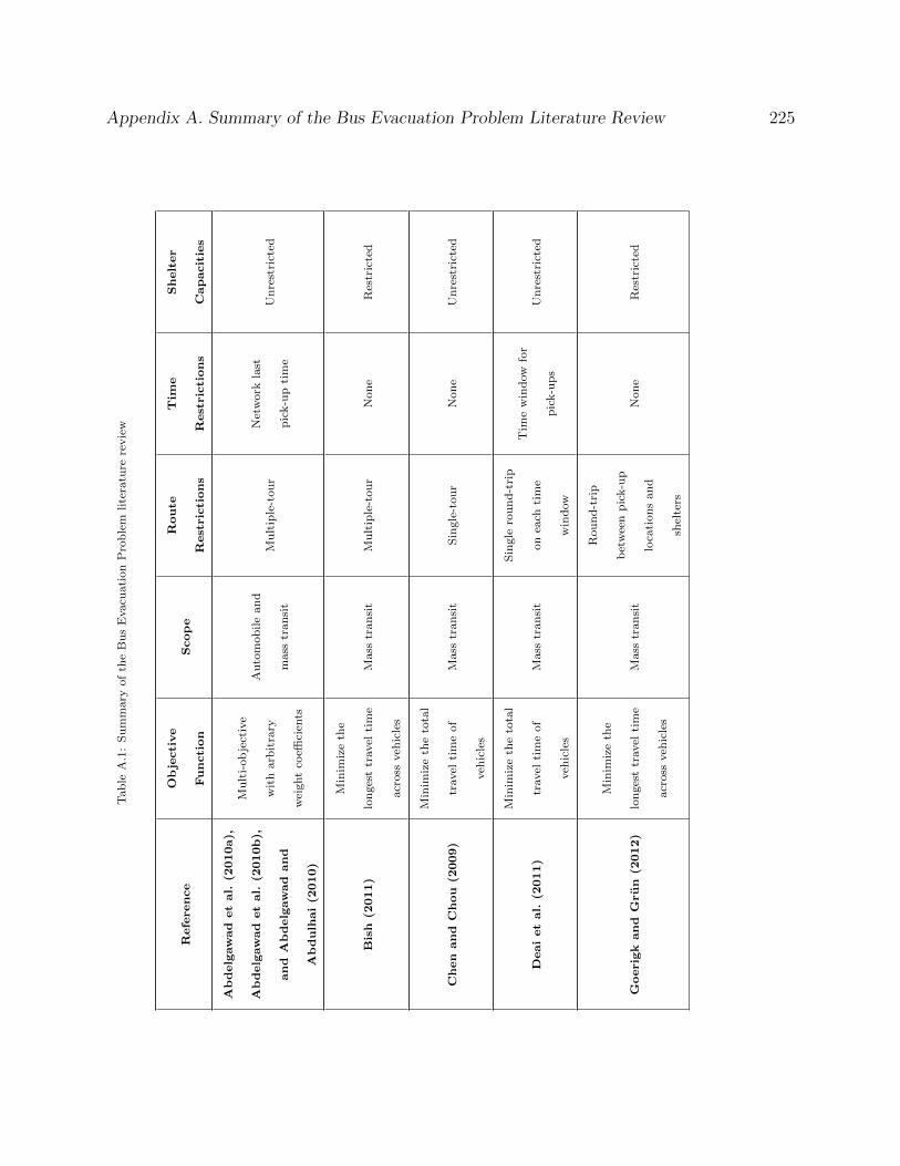
Appendix A. Summary of the Bus Evacuation Problem Literature Review 225T
ab
leA
.1:
Su
mm
ary
of
the
Bu
sE
vacu
ati
on
Pro
ble
mlite
ratu
rere
vie
w
Reference
Objective
Function
Scope
Route
Restrictions
Tim
e
Restrictions
Shelter
Capacities
Abdelgawad
etal.
(2010a),
Abdelgawad
etal.
(2010b),
and
Abdelgawad
and
Abdulh
ai(2
010)
Mu
lti-
ob
ject
ive
wit
harb
itra
ry
wei
ght
coeffi
cien
ts
Au
tom
ob
ile
an
d
mass
tran
sit
Mu
ltip
le-t
ou
rN
etw
ork
last
pic
k-u
pti
me
Un
rest
rict
ed
Bish
(2011)
Min
imiz
eth
e
lon
ges
ttr
avel
tim
e
acr
oss
veh
icle
s
Mass
tran
sit
Mu
ltip
le-t
ou
rN
on
eR
estr
icte
d
Chen
and
Chou
(2009)
Min
imiz
eth
eto
tal
travel
tim
eof
veh
icle
s
Mass
tran
sit
Sin
gle
-tou
rN
on
eU
nre
stri
cted
Deaietal.
(2011)
Min
imiz
eth
eto
tal
travel
tim
eof
veh
icle
s
Mass
tran
sit
Sin
gle
rou
nd
-tri
p
on
each
tim
e
win
dow
Tim
ew
ind
ow
for
pic
k-u
ps
Un
rest
rict
ed
Goerigk
and
Grun
(2012)
Min
imiz
eth
e
lon
ges
ttr
avel
tim
e
acr
oss
veh
icle
s
Mass
tran
sit
Rou
nd
-tri
p
bet
wee
np
ick-u
p
loca
tion
san
d
shel
ters
Non
eR
estr
icte
d
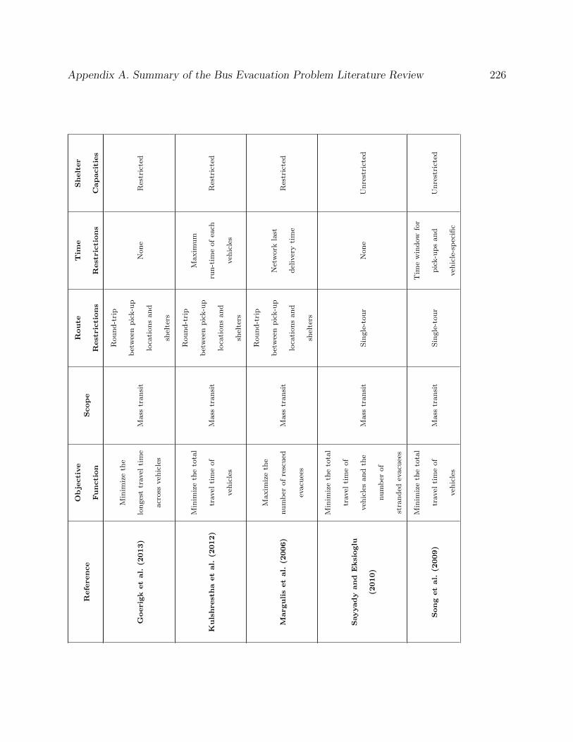
Appendix A. Summary of the Bus Evacuation Problem Literature Review 226Reference
Objective
Function
Scope
Route
Restrictions
Tim
e
Restrictions
Shelter
Capacities
Goerigk
etal.
(2013)
Min
imiz
eth
e
lon
ges
ttr
avel
tim
e
acr
oss
veh
icle
s
Mass
tran
sit
Rou
nd
-tri
p
bet
wee
np
ick-u
p
loca
tion
san
d
shel
ters
Non
eR
estr
icte
d
Kulshrestha
etal.
(2012)
Min
imiz
eth
eto
tal
travel
tim
eof
veh
icle
s
Mass
tran
sit
Rou
nd
-tri
p
bet
wee
np
ick-u
p
loca
tion
san
d
shel
ters
Maxim
um
run
-tim
eof
each
veh
icle
s
Res
tric
ted
Margulisetal.
(2006)
Maxim
ize
the
num
ber
of
resc
ued
evacu
ees
Mass
tran
sit
Rou
nd
-tri
p
bet
wee
np
ick-u
p
loca
tion
san
d
shel
ters
Net
work
last
del
iver
yti
me
Res
tric
ted
Sayyady
and
Eksioglu
(2010)
Min
imiz
eth
eto
tal
travel
tim
eof
veh
icle
san
dth
e
nu
mb
erof
stra
nd
edev
acu
ees
Mass
tran
sit
Sin
gle
-tou
rN
on
eU
nre
stri
cted
Song
etal.
(2009)
Min
imiz
eth
eto
tal
travel
tim
eof
veh
icle
s
Mass
tran
sit
Sin
gle
-tou
r
Tim
ew
ind
ow
for
pic
k-u
ps
an
d
veh
icle
-sp
ecifi
c
Un
rest
rict
ed
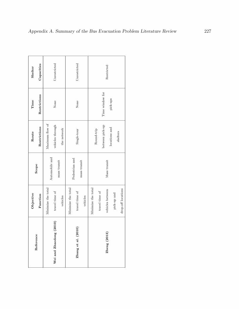
Appendix A. Summary of the Bus Evacuation Problem Literature Review 227Reference
Objective
Function
Scope
Route
Restrictions
Tim
e
Restrictions
Shelter
Capacities
Weiand
Zhaodong
(2010)
Min
imiz
eth
eto
tal
travel
tim
eof
veh
icle
s
Au
tom
ob
ile
an
d
mass
tran
sit
Maxim
um
flow
of
veh
icle
sth
rou
gh
the
net
work
Non
eU
nre
stri
cted
Zhang
etal.
(2010)
Min
imiz
eth
eto
tal
travel
tim
eof
veh
icle
s
Ped
estr
ian
an
d
mass
tran
sit
Sin
gle
-tou
rN
on
eU
nre
stri
cted
Zheng
(2013)
Min
imiz
eth
eto
tal
travel
tim
eof
veh
icle
sb
etw
een
pic
k-u
pan
d
dro
p-o
fflo
cati
on
s
Mass
tran
sit
Rou
nd
-tri
p
bet
wee
np
ick-u
p
loca
tion
san
d
shel
ters
Tim
ew
ind
ow
for
pic
k-u
ps
Res
tric
ted
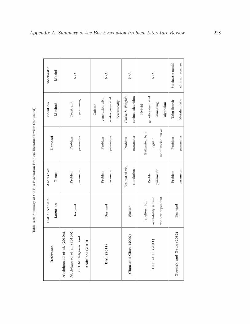
Appendix A. Summary of the Bus Evacuation Problem Literature Review 228T
ab
leA
.2:
Su
mm
ary
of
the
Bu
sE
vacu
ati
on
Pro
ble
mlite
ratu
rere
vie
w(c
onti
nu
ed)
Reference
InitialVehicle
Location
ArcTravel
Tim
es
Dem
and
Solu
tion
Meth
od
Sto
chastic
Model
Abdelgawad
etal.
(2010a),
Abdelgawad
etal.
(2010b),
and
Abdelgawad
and
Abdulh
ai(2
010)
Bu
syard
Pro
ble
m
para
met
er
Pro
ble
m
para
met
er
Con
stra
int
pro
gra
mm
ing
N/A
Bish
(2011)
Bu
syard
Pro
ble
m
para
met
er
Pro
ble
m
para
met
er
Colu
mn
gen
erati
on
wit
h
rou
tes
gen
erate
d
heu
rist
ically
N/A
Chen
and
Chou
(2009)
Sh
elte
rsE
stim
ate
dvia
sim
ula
tion
Pro
ble
m
para
met
er
Cla
rke
&W
right’
s
savin
gs
alg
ori
thm
N/A
Deaietal.
(2011)
Sh
elte
rs,
bu
t
availab
ilit
yis
tim
e
win
dow
dep
end
ent
Pro
ble
m
para
met
er
Est
imate
dby
a
logis
tic
mob
iliz
ati
on
curv
e
Hyb
rid
gen
etic
/si
mu
late
d
an
nea
lin
g
alg
ori
thm
N/A
Goerigk
and
Grun
(2012)
Bu
syard
Pro
ble
m
para
met
er
Pro
ble
m
para
met
er
Tab
uS
earc
h
Met
ah
euri
stic
Sto
chast
icm
od
el
wit
hn
ore
cou
rse
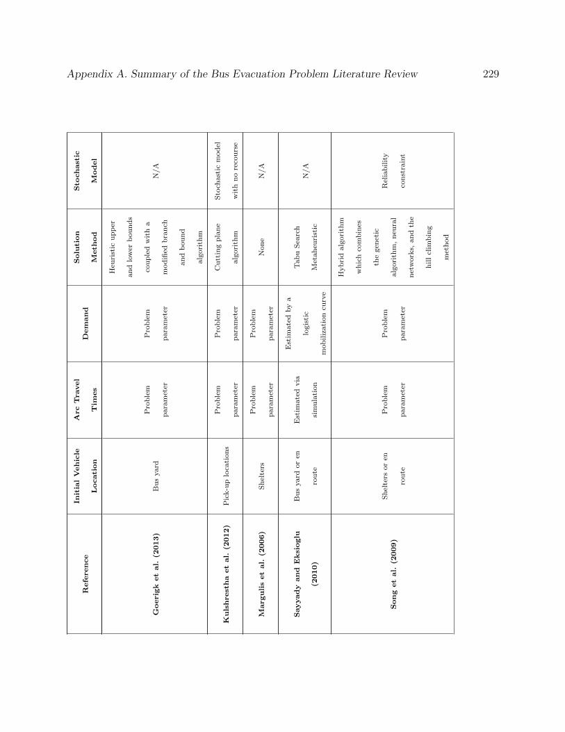
Appendix A. Summary of the Bus Evacuation Problem Literature Review 229Reference
InitialVehicle
Location
ArcTravel
Tim
es
Dem
and
Solu
tion
Meth
od
Sto
chastic
Model
Goerigk
etal.
(2013)
Bu
syard
Pro
ble
m
para
met
er
Pro
ble
m
para
met
er
Heu
rist
icu
pp
er
an
dlo
wer
bou
nd
s
cou
ple
dw
ith
a
mod
ified
bra
nch
an
db
oun
d
alg
ori
thm
N/A
Kulshrestha
etal.
(2012)
Pic
k-u
plo
cati
on
sP
rob
lem
para
met
er
Pro
ble
m
para
met
er
Cu
ttin
gp
lan
e
alg
ori
thm
Sto
chast
icm
od
el
wit
hn
ore
cou
rse
Margulisetal.
(2006)
Sh
elte
rsP
rob
lem
para
met
er
Pro
ble
m
para
met
erN
on
eN
/A
Sayyady
and
Eksioglu
(2010)
Bu
syard
or
en
rou
te
Est
imate
dvia
sim
ula
tion
Est
imate
dby
a
logis
tic
mob
iliz
ati
on
curv
e
Tab
uS
earc
h
Met
ah
euri
stic
N/A
Song
etal.
(2009)
Sh
elte
rsor
en
rou
te
Pro
ble
m
para
met
er
Pro
ble
m
para
met
er
Hyb
rid
alg
ori
thm
wh
ich
com
bin
es
the
gen
etic
alg
ori
thm
,n
eura
l
net
work
s,an
dth
e
hill
clim
bin
g
met
hod
Rel
iab
ilit
y
con
stra
int

Appendix A. Summary of the Bus Evacuation Problem Literature Review 230Reference
InitialVehicle
Location
ArcTravel
Tim
es
Dem
and
Solu
tion
Meth
od
Sto
chastic
Model
Weiand
Zhaodong
(2010)
Pic
k-u
plo
cati
on
s
Pro
ble
m
para
met
er.
Als
o
ass
um
esm
axim
um
road
cap
aci
ty
Pro
ble
m
para
met
er
Rel
axati
on
stra
tegy
N/A
Zhang
etal.
(2010)
Sh
elte
rs
Pro
bab
ilis
tic
effec
t
of
ped
estr
ian
traffi
con
mass
tran
sit
veh
icle
spee
d
Est
imate
dby
a
logis
tic
mob
iliz
ati
on
curv
e
Dij
kst
ra’s
alg
ori
thm
N/A
Zheng
(2013)
Bu
syard
or
en
rou
te
Pro
ble
m
para
met
er
Pro
ble
m
para
met
er
Lagra
ngia
n
rela
xati
on
cou
ple
d
wit
hre
form
ula
tion
into
MC
NF
P
N/A
Appendix B
Alternative Formulations for the Bus
Evacuation Problem with Constant
Evacuee Arrival Rate
231

Appendix B. Alternative Formulations for the BEP with Const. Evac. Arrival Rate 232
This section reiterates the modeling notation and introduces alternative formulations to the
BEP variant introduced in Chapter 2.
B.1 Original Formulation in Standard Form
Consider the complete network (N,A), where N and A are the set of nodes and arcs, re-
spectively. The set N consists of set P , the set of pick-up locations (each one located on a
neighborhood requiring evacuation services), and node 0, the depot, which, for simplicity,
also functions as a shelter. Each arc (i, j) ∈ A has an associated arc traversal time, tij,
satisfying the triangle inequality, that is, tij ≤ tik + tkj, ∀ (i, j), (i, k), and (k, j) ∈ A. Each
pick-up location j ∈ P has an associated constant evacuee arrival rate, Dj, and a last sched-
uled pick-up time, Lj, which also corresponds to the end of the evacuee arrival process on
this node. Consequently, each pick-up location has total demand of DjLj evacuees. Finally,
let F be the maximum number of scheduled pick-ups on each pick-up location (service level);
let T (F ) be an upper bound on the number of arc traversals for each vehicle; and let V be
the number of buses available for the evacuation, each with capacity for C evacuees. Table
B.1 presents the decision variables for the BEP variant introduced in Chapter 2.
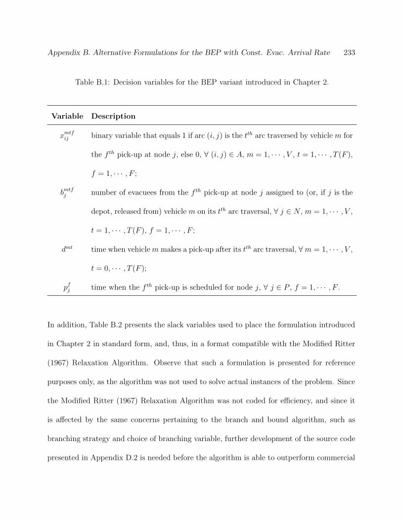
Appendix B. Alternative Formulations for the BEP with Const. Evac. Arrival Rate 233
Table B.1: Decision variables for the BEP variant introduced in Chapter 2.
Variable Description
xmtfij binary variable that equals 1 if arc (i, j) is the tth arc traversed by vehicle m for
the f th pick-up at node j, else 0, ∀ (i, j) ∈ A, m = 1, · · · , V , t = 1, · · · , T (F ),
f = 1, · · · , F ;
bmtfj number of evacuees from the f th pick-up at node j assigned to (or, if j is the
depot, released from) vehicle m on its tth arc traversal, ∀ j ∈ N , m = 1, · · · , V ,
t = 1, · · · , T (F ), f = 1, · · · , F ;
dmt time when vehicle m makes a pick-up after its tth arc traversal, ∀m = 1, · · · , V ,
t = 0, · · · , T (F );
pfj time when the f th pick-up is scheduled for node j, ∀ j ∈ P , f = 1, · · · , F .
In addition, Table B.2 presents the slack variables used to place the formulation introduced
in Chapter 2 in standard form, and, thus, in a format compatible with the Modified Ritter
(1967) Relaxation Algorithm. Observe that such a formulation is presented for reference
purposes only, as the algorithm was not used to solve actual instances of the problem. Since
the Modified Ritter (1967) Relaxation Algorithm was not coded for efficiency, and since it
is affected by the same concerns pertaining to the branch and bound algorithm, such as
branching strategy and choice of branching variable, further development of the source code
presented in Appendix D.2 is needed before the algorithm is able to outperform commercial

Appendix B. Alternative Formulations for the BEP with Const. Evac. Arrival Rate 234
optimization packages such as IBM ILOG CPLEX.
Table B.2: Slack variables for the formulation introduced in Chapter 2.
Variable Description
C3mt slack variable that equals 1 if vehicle m visits and parks at the depot after its
tth arc traversal, else 0, ∀ m = 1, · · · , V, t = 1, · · · , T (F )− 1;
C5mt slack variable that equals 1 if vehicle m does not perform a pick-up after its tth
arc traversal (i.e., if the vehicle either visits the depot or bypasses a pick-up
node without stopping), else 0, ∀ m = 1, · · · , V, t = 1, · · · , T (F );
C6mt slack variable corresponding to the amount of time vehicle m remains idle after
its tth arc traversal, ∀ m = 1, · · · , V, t = 1, · · · , T (F );
C7mtfj slack variable corresponding to the delay between the departure time of vehicle
m from node j after its tth arc traversal and the f th scheduled pick-up time for
this node, assuming that such a vehicle performs this pick-up, else unrestricted,
∀ j ∈ P, m = 1, · · · , V, t = 1, · · · , T (F ), f = 1, · · · , F ;
C8mtfj slack variable corresponding to the lead time between vehicle m departure from
node j after its tth arc traversal and the f th scheduled pick-up time for this
node, assuming that such a vehicle is performs this pick-up, else unrestricted,
∀ j ∈ P, m = 1, · · · , V, t = 1, · · · , T (F ), f = 1, · · · , F ;
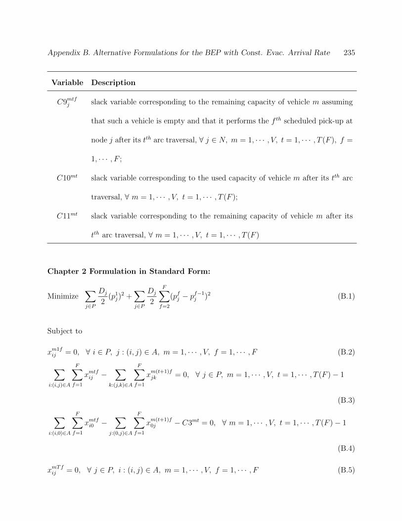
Appendix B. Alternative Formulations for the BEP with Const. Evac. Arrival Rate 235
Variable Description
C9mtfj slack variable corresponding to the remaining capacity of vehicle m assuming
that such a vehicle is empty and that it performs the f th scheduled pick-up at
node j after its tth arc traversal, ∀ j ∈ N, m = 1, · · · , V, t = 1, · · · , T (F ), f =
1, · · · , F ;
C10mt slack variable corresponding to the used capacity of vehicle m after its tth arc
traversal, ∀ m = 1, · · · , V, t = 1, · · · , T (F );
C11mt slack variable corresponding to the remaining capacity of vehicle m after its
tth arc traversal, ∀ m = 1, · · · , V, t = 1, · · · , T (F )
Chapter 2 Formulation in Standard Form:
Minimize∑
j∈P
Dj
2(p1j)
2 +∑
j∈P
Dj
2
F∑
f=2
(pfj − pf−1j )2 (B.1)
Subject to
xm1fij = 0, ∀ i ∈ P, j : (i, j) ∈ A, m = 1, · · · , V, f = 1, · · · , F (B.2)
∑
i:(i,j)∈A
F∑
f=1
xmtfij −∑
k:(j,k)∈A
F∑
f=1
xm(t+1)fjk = 0, ∀ j ∈ P, m = 1, · · · , V, t = 1, · · · , T (F )− 1
(B.3)
∑
i:(i,0)∈A
F∑
f=1
xmtfi0 −∑
j:(0,j)∈A
F∑
f=1
xm(t+1)f0j − C3mt = 0, ∀ m = 1, · · · , V, t = 1, · · · , T (F )− 1
(B.4)
xmTfij = 0, ∀ j ∈ P, i : (i, j) ∈ A, m = 1, · · · , V, f = 1, · · · , F (B.5)

Appendix B. Alternative Formulations for the BEP with Const. Evac. Arrival Rate 236
xmtfi0 = 0, ∀ i : (i, 0) ∈ A, m = 1, · · · , V, t = 1, · · · , T (F ), f = 2, · · · , F (B.6)
∑
(i,j)∈A
F∑
f=1
xmtfij + C5mt = 1, ∀ m = 1, · · · , V, t = 1, · · · , T (F ) (B.7)
dm0 = 0, ∀ m = 1, · · · , V (B.8)
∑
(i,j)∈A
F∑
f=1
tijxmtfij + dm(t−1) − dmt + C6mt = 0, ∀ m = 1, · · · , V, t = 1, · · · , T (F ) (B.9)
∑
i:(i,j)∈A
M xmtfij − dmt + C7mtfj + pfj = M, ∀ j ∈ P, m = 1, · · · , V, t = 1, · · · , T (F ), f = 1, · · · , F
(B.10)
∑
i:(i,j)∈A
M xmtfij + dmt + C8mtfj − pfj = M, ∀ j ∈ P, m = 1, · · · , V, t = 1, · · · , T (F ), f = 1, · · · , F
(B.11)
bmtf0 = 0, ∀ m = 1, · · · , V, t = 1, · · · , T (F ), f = 2, · · · , F (B.12)
∑
i:(i,j)∈A
Cxmtfij − bmtfj − C9mtfj = 0, ∀ j ∈ N, m = 1, · · · , V, t = 1, · · · , T (F ), f = 1, · · · , F
(B.13)
t∑
l=1
F∑
f=1
bmlf0 −∑
j∈P
t∑
l=1
F∑
f=1
bmlfj + C10mt = 0, ∀ m = 1, · · · , V, t = 1, · · · , T (F ) (B.14)
t∑
l=1
F∑
f=1
bmlf0 −∑
j∈P
t∑
l=1
F∑
f=1
bmlfj − C11mt = −C, ∀ m = 1, · · · , V, t = 1, · · · , T (F ) (B.15)
V∑
m=1
T (F )∑
t=1
bmt1j −Dj p1j = 0, ∀ j ∈ P (B.16)
V∑
m=1
T (F )∑
t=1
bmtfj +Dj pf−1j −Dj p
fj = 0, ∀ j ∈ P, f = 2, · · · , F (B.17)
pFj = Lj, ∀ j ∈ P. (B.18)
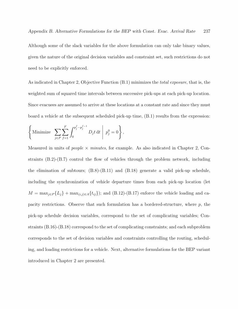
Appendix B. Alternative Formulations for the BEP with Const. Evac. Arrival Rate 237
Although some of the slack variables for the above formulation can only take binary values,
given the nature of the original decision variables and constraint set, such restrictions do not
need to be explicitly enforced.
As indicated in Chapter 2, Objective Function (B.1) minimizes the total exposure, that is, the
weighted sum of squared time intervals between successive pick-ups at each pick-up location.
Since evacuees are assumed to arrive at these locations at a constant rate and since they must
board a vehicle at the subsequent scheduled pick-up time, (B.1) results from the expression:
{Minimize
∑
j∈P
F∑
f=1
∫ pfj−pf−1j
0
Djt dt
∣∣∣∣∣ p0j = 0
},
Measured in units of people × minutes, for example. As also indicated in Chapter 2, Con-
straints (B.2)-(B.7) control the flow of vehicles through the problem network, including
the elimination of subtours; (B.8)-(B.11) and (B.18) generate a valid pick-up schedule,
including the synchronization of vehicle departure times from each pick-up location (let
M = maxj∈P{Lj} + max(i,j)∈A{tij}); and (B.12)-(B.17) enforce the vehicle loading and ca-
pacity restrictions. Observe that such formulation has a bordered-structure, where p, the
pick-up schedule decision variables, correspond to the set of complicating variables; Con-
straints (B.16)-(B.18) correspond to the set of complicating constraints; and each subproblem
corresponds to the set of decision variables and constraints controlling the routing, schedul-
ing, and loading restrictions for a vehicle. Next, alternative formulations for the BEP variant
introduced in Chapter 2 are presented.
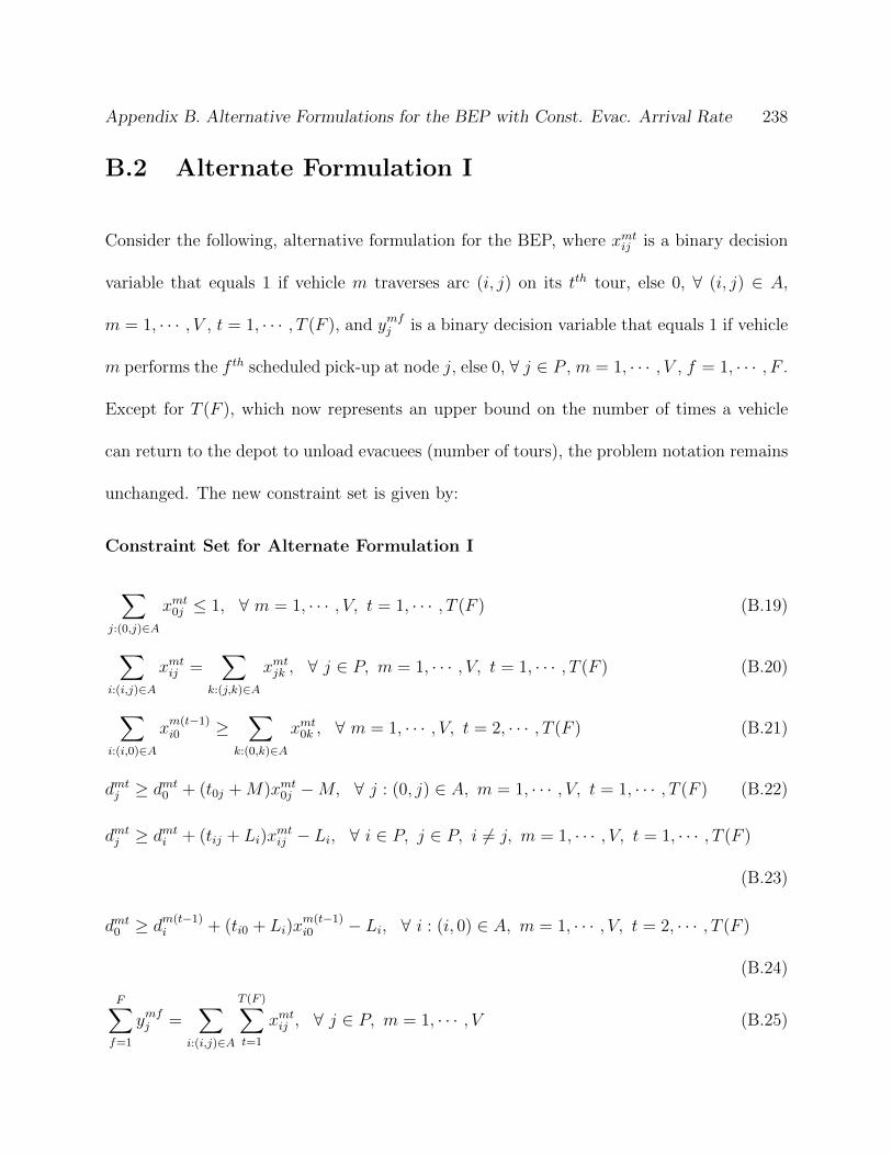
Appendix B. Alternative Formulations for the BEP with Const. Evac. Arrival Rate 238
B.2 Alternate Formulation I
Consider the following, alternative formulation for the BEP, where xmtij is a binary decision
variable that equals 1 if vehicle m traverses arc (i, j) on its tth tour, else 0, ∀ (i, j) ∈ A,
m = 1, · · · , V , t = 1, · · · , T (F ), and ymfj is a binary decision variable that equals 1 if vehicle
m performs the f th scheduled pick-up at node j, else 0, ∀ j ∈ P , m = 1, · · · , V , f = 1, · · · , F .
Except for T (F ), which now represents an upper bound on the number of times a vehicle
can return to the depot to unload evacuees (number of tours), the problem notation remains
unchanged. The new constraint set is given by:
Constraint Set for Alternate Formulation I
∑
j:(0,j)∈A
xmt0j ≤ 1, ∀ m = 1, · · · , V, t = 1, · · · , T (F ) (B.19)
∑
i:(i,j)∈A
xmtij =∑
k:(j,k)∈A
xmtjk , ∀ j ∈ P, m = 1, · · · , V, t = 1, · · · , T (F ) (B.20)
∑
i:(i,0)∈A
xm(t−1)i0 ≥
∑
k:(0,k)∈A
xmt0k , ∀ m = 1, · · · , V, t = 2, · · · , T (F ) (B.21)
dmtj ≥ dmt0 + (t0j +M)xmt0j −M, ∀ j : (0, j) ∈ A, m = 1, · · · , V, t = 1, · · · , T (F ) (B.22)
dmtj ≥ dmti + (tij + Li)xmtij − Li, ∀ i ∈ P, j ∈ P, i 6= j, m = 1, · · · , V, t = 1, · · · , T (F )
(B.23)
dmt0 ≥ dm(t−1)i + (ti0 + Li)x
m(t−1)i0 − Li, ∀ i : (i, 0) ∈ A, m = 1, · · · , V, t = 2, · · · , T (F )
(B.24)
F∑
f=1
ymfj =∑
i:(i,j)∈A
T (F )∑
t=1
xmtij , ∀ j ∈ P, m = 1, · · · , V (B.25)
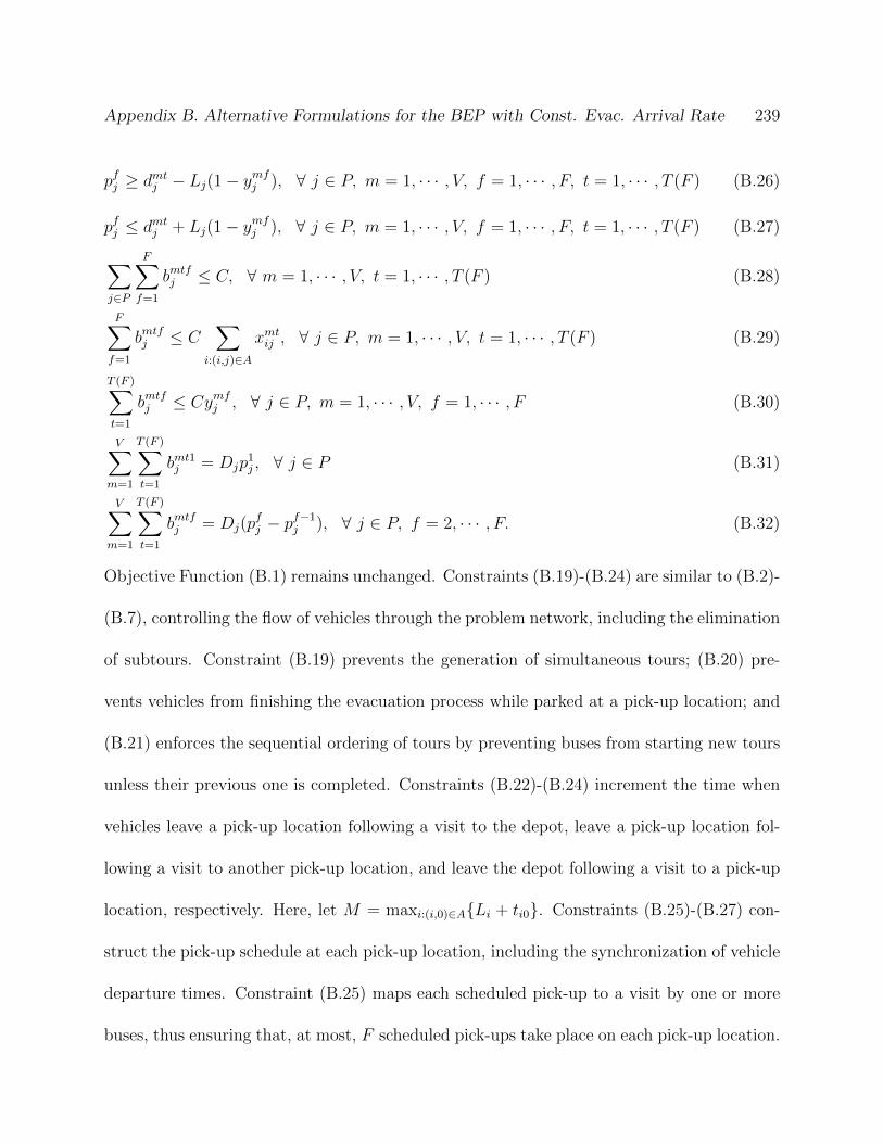
Appendix B. Alternative Formulations for the BEP with Const. Evac. Arrival Rate 239
pfj ≥ dmtj − Lj(1− ymfj ), ∀ j ∈ P, m = 1, · · · , V, f = 1, · · · , F, t = 1, · · · , T (F ) (B.26)
pfj ≤ dmtj + Lj(1− ymfj ), ∀ j ∈ P, m = 1, · · · , V, f = 1, · · · , F, t = 1, · · · , T (F ) (B.27)
∑
j∈P
F∑
f=1
bmtfj ≤ C, ∀ m = 1, · · · , V, t = 1, · · · , T (F ) (B.28)
F∑
f=1
bmtfj ≤ C∑
i:(i,j)∈A
xmtij , ∀ j ∈ P, m = 1, · · · , V, t = 1, · · · , T (F ) (B.29)
T (F )∑
t=1
bmtfj ≤ Cymfj , ∀ j ∈ P, m = 1, · · · , V, f = 1, · · · , F (B.30)
V∑
m=1
T (F )∑
t=1
bmt1j = Djp1j , ∀ j ∈ P (B.31)
V∑
m=1
T (F )∑
t=1
bmtfj = Dj(pfj − pf−1
j ), ∀ j ∈ P, f = 2, · · · , F. (B.32)
Objective Function (B.1) remains unchanged. Constraints (B.19)-(B.24) are similar to (B.2)-
(B.7), controlling the flow of vehicles through the problem network, including the elimination
of subtours. Constraint (B.19) prevents the generation of simultaneous tours; (B.20) pre-
vents vehicles from finishing the evacuation process while parked at a pick-up location; and
(B.21) enforces the sequential ordering of tours by preventing buses from starting new tours
unless their previous one is completed. Constraints (B.22)-(B.24) increment the time when
vehicles leave a pick-up location following a visit to the depot, leave a pick-up location fol-
lowing a visit to another pick-up location, and leave the depot following a visit to a pick-up
location, respectively. Here, let M = maxi:(i,0)∈A{Li + ti0}. Constraints (B.25)-(B.27) con-
struct the pick-up schedule at each pick-up location, including the synchronization of vehicle
departure times. Constraint (B.25) maps each scheduled pick-up to a visit by one or more
buses, thus ensuring that, at most, F scheduled pick-ups take place on each pick-up location.

Appendix B. Alternative Formulations for the BEP with Const. Evac. Arrival Rate 240
Constraints (B.26)-(B.27) map vehicle departure times to scheduled pick-up times and en-
force a sequential pick-up schedule (i.e., they imply that pfj ≥ pf−1j , ∀ j ∈ P, f = 1, · · · , F ).
Finally, (B.28) enforces vehicle capacity restrictions; (B.29)-(B.30) prevent evacuees from
boarding vehicles unless these are visiting the corresponding pick-up location; and (B.31)-
(B.32) ensure that every new arrival boards a vehicle on the next scheduled pick-up time. In
addition, Constraints (B.8) and (B.18) and the logical binary and non-negativity restrictions
are included.
In the formulation introduced in Chapter 2, a variable index tracks each arc traversal through
the problem network. Therefore, the formulation allows buses to visit the same pick-up
location multiple times during the same tour, that is, it allows the construction of transit
corridors. Such phenomenon is not necessarily problematic, and, in fact, may even be desired
during the operation of real-life transit systems. However, in evacuation settings, such
phenomenon may increase the average riding time of evacuees, as shown in Example B.1.
Example B.1 Consider the network displayed in Figure B.1(a), with parameters F = 2
pick-ups, V = 1 bus, and C = 20 evacuees/bus. Figures B.1(b) and B.1(c) depict, respec-
tively, the optimal pick-up schedules assuming that the construction of transit corridors is
allowed (at time p11 = 1, p2
1 = L1 = 5, p12 = 2, p2
2 = L2 = 4, and p13 = L3 = 3) and not al-
lowed (at time p11 = L1 = 5, p1
2 = L2 = 4, and p13 = L3 = 3). In these figures, solid lines are
used to represent time periods when buses are idle, whereas dashed lines to represent periods
when buses are moving. The number of evacuees on each bus, if any, is presented on top
of the dashed lines. Since the formulation prevents the construction of transit corridors, it
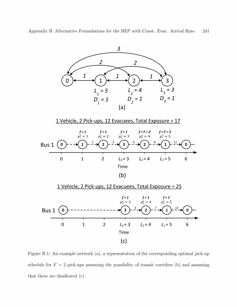
Appendix B. Alternative Formulations for the BEP with Const. Evac. Arrival Rate 241
1 Vehicle, 2 Pick-ups, 12 Evacuees, Total Exposure = 17
f = F = 2 f = 1
Bus 1 0 0 1 1
Time
(b)
1 8 12 3
f = 1
f = 1
1 L3 = 3 L2 = 4 0 6 2 L1 = 5
2 3 2 6
f = F = 2
3
2 1
2
L2 = 4
D2 = 1
(a)
0 1 1
L1 = 5
D1 = 1
3 1
L3 = 3
D3 = 1
2
1 Vehicle, 2 Pick-ups, 12 Evacuees, Total Exposure = 25
f = 1
f = 1
Bus 1 0 0 1
Time
(c)
7 12
1 L3 = 3 L2 = 4 0 6 2 L1 = 5
3 2 3
f = 1
Figure B.1: An example network (a), a representation of the corresponding optimal pick-up
schedule for F = 2 pick-ups assuming the possibility of transit corridors (b) and assuming
that these are disallowed (c).
Appendix B. Alternative Formulations for the BEP with Const. Evac. Arrival Rate 242
restricts the problem feasible region, thus potentially leading to infeasibility or to larger objec-
tive function values. In this example, the proposed formulation led to an increase in objective
function value from 17 to 25 people × minutes. Nonetheless, such increase was accompanied
by a concomitant reduction in total riding time, from 30 to 22 people × minutes.
Finally, observe that such formulation still maintains the bordered-structure of the origi-
nal formulation, where p, the pick-up schedule decision variables, correspond to the set of
complicating variables; Constraints (B.31)-(B.32) and (B.18) correspond to the set of com-
plicating constraints; and each subproblem corresponds to the set of decision variables and
constraints controlling the routing, scheduling, and loading restrictions for a vehicle.
B.3 Alternate Formulation II
While the formulation proposed in Section B.2 considerably restricts the search space for
the problem, such can be further reduced by noting, from (B.31)-(B.32), that:
p1j = 1
Dj
∑Vm=1
∑T (F )t=1 bmt1j , ∀ j ∈ P,
pfj − pf−1j = 1
Dj
∑Vm=1
∑T (F )t=1 bmtfj , ∀ j ∈ P, f = 2, · · · , F
⇔ pfj =1
Dj
V∑
m=1
f∑
l=1
T (F )∑
t=1
bmtlj , ∀ j ∈ P, f = 1, · · · , F
Consequently, such constraints and the respective decision variables can be eliminated by
performing the appropriate substitutions. In the new formulation, (B.8), (B.19)-(B.25), and
(B.28)-(B.30) remain unchanged; (B.26)-(B.27) are replaced by (B.34)-(B.35); (B.31)-(B.32)
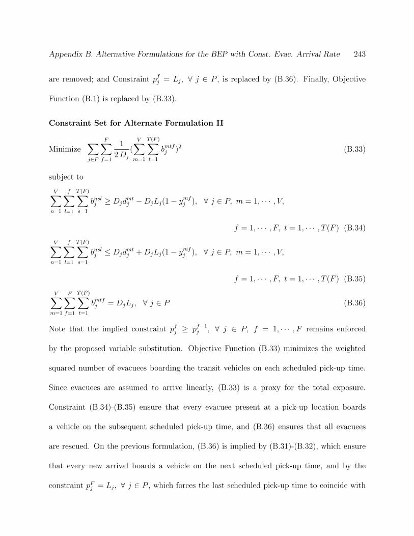
Appendix B. Alternative Formulations for the BEP with Const. Evac. Arrival Rate 243
are removed; and Constraint pfj = Lj, ∀ j ∈ P , is replaced by (B.36). Finally, Objective
Function (B.1) is replaced by (B.33).
Constraint Set for Alternate Formulation II
Minimize∑
j∈P
F∑
f=1
1
2Dj
(V∑
m=1
T (F )∑
t=1
bmtfj )2 (B.33)
subject to
V∑
n=1
f∑
l=1
T (F )∑
s=1
bnslj ≥ Djdmtj −DjLj(1− ymfj ), ∀ j ∈ P, m = 1, · · · , V,
f = 1, · · · , F, t = 1, · · · , T (F ) (B.34)
V∑
n=1
f∑
l=1
T (F )∑
s=1
bnslj ≤ Djdmtj +DjLj(1− ymfj ), ∀ j ∈ P, m = 1, · · · , V,
f = 1, · · · , F, t = 1, · · · , T (F ) (B.35)
V∑
m=1
F∑
f=1
T (F )∑
t=1
bmtfj = DjLj, ∀ j ∈ P (B.36)
Note that the implied constraint pfj ≥ pf−1j , ∀ j ∈ P, f = 1, · · · , F remains enforced
by the proposed variable substitution. Objective Function (B.33) minimizes the weighted
squared number of evacuees boarding the transit vehicles on each scheduled pick-up time.
Since evacuees are assumed to arrive linearly, (B.33) is a proxy for the total exposure.
Constraint (B.34)-(B.35) ensure that every evacuee present at a pick-up location boards
a vehicle on the subsequent scheduled pick-up time, and (B.36) ensures that all evacuees
are rescued. On the previous formulation, (B.36) is implied by (B.31)-(B.32), which ensure
that every new arrival boards a vehicle on the next scheduled pick-up time, and by the
constraint pFj = Lj, ∀ j ∈ P , which forces the last scheduled pick-up time to coincide with

Appendix B. Alternative Formulations for the BEP with Const. Evac. Arrival Rate 244
the end of the evacuee arrival process. Interestingly, by eliminating the pick-up scheduling
variables, the inheriting bordered-structure of the problem change to a block diagonal or
angular structure, where each subproblem remains the tour for one of the available buses,
and the complicating constraints change to the allocation of evacuees to individual vehicles.
Although such formulation has a simpler structure, empirical studies have demonstrated
that the ensuing increase in the number of non-zero coefficients (problem density) leads to
an increase in solution time. Nonetheless, such formulation allows the problem to be solved
by Dantzig-Wolfe Decomposition (Dantzig and Wolfe, 1960), or, in turn, its dual problem
solved by Benders’ Decomposition (Benders, 1962). Research is needed to determine whether
such algorithms, when used to solve such a dual angular formulation of the aforementioned
BEP variant, are able to attain faster computation times than the Modified Ritter (1967)
Relaxation Algorithm applied the original problem.
B.4 Alternate Formulation III
Alternatively, consider the following formulation which, similar to the one introduced in
Chapter 2, combines the decision variables xmtij and ymfj into a single, binary decision variable,
zmtfij , that equals 1 if arc (i, j) is traversed by vehicle m on its tth tour for the f th pick-up at
node j, else 0, ∀ (i, j) ∈ A, m = 1, · · · , V, f = 1, · · · , F, t = 1, · · · , T (F ). For notational
simplicity, the depot variables zmtfi0 use the same index f as the ones for the pick-up nodes,
but they are set to zero for pick-ups f = 2, · · · , F (i.e., let zmtfi0 = 0, ∀ i : (i, 0) ∈ A, m =

Appendix B. Alternative Formulations for the BEP with Const. Evac. Arrival Rate 245
1, · · · , V, f = 2, · · · , F, t = 1, · · · , T (F )). Similar to the previous alternate formulations, the
subscript t denotes the tour index rather than the arc traversal index, and the construction
of transit corridors is prevented by the proposed constraint set.
Constraint Set for Alternate Formulation III
∑
j:(0,j)∈A
F∑
f=1
zmtf0j ≤ 1, ∀ m = 1, · · · , V, t = 1, · · · , T (F ) (B.37)
∑
i:(i,j)∈A
F∑
f=1
zmtfij =∑
k:(j,k)∈A
F∑
f=1
zmtfjk , ∀ j ∈ P, m = 1, · · · , V, t = 1, · · · , T (F ) (B.38)
∑
i:(i,0)∈A
zm1(t−1)i0 ≥
∑
k:(0,k)∈A
F∑
f=1
zmtf0k , ∀ m = 1, · · · , V, t = 2, · · · , T (F ) (B.39)
dmtj ≥ dmt0 + (t0j +M)F∑
f=1
zmtf0j −M, ∀ j : (0, j) ∈ A, m = 1, · · · , V, t = 1, · · · , T (F )
(B.40)
dmtj ≥ dmti + (tij + Li)F∑
f=1
zmtfij − Li, ∀ i ∈ P, j ∈ P, i 6= j, m = 1, · · · , V, t = 1, · · · , T (F )
(B.41)
dmt0 ≥ dm(t−1)i + (ti0 + Li)z
m(t−1)1i0 − Li, ∀ i : (i, 0) ∈ A, m = 1, · · · , V, t = 2, · · · , T (F )
(B.42)
pfj ≥ dmtj − Lj(1−∑
i:(i,j)∈A
zmtfij ), ∀ j ∈ P, m = 1, · · · , V, f = 1, · · · , F, t = 1, · · · , T (F )
(B.43)
pfj ≤ dmtj + Lj(1−∑
i:(i,j)∈A
zmtfij ), ∀ j ∈ P, m = 1, · · · , V, f = 1, · · · , F, t = 1, · · · , T (F )
(B.44)
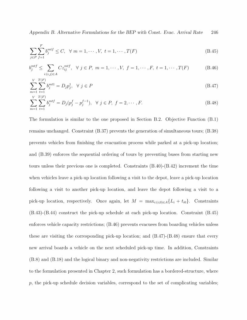
Appendix B. Alternative Formulations for the BEP with Const. Evac. Arrival Rate 246
∑
j∈P
F∑
f=1
bmtfj ≤ C, ∀ m = 1, · · · , V, t = 1, · · · , T (F ) (B.45)
bmtfj ≤∑
i:(i,j)∈A
Czmtfij , ∀ j ∈ P, m = 1, · · · , V, f = 1, · · · , F, t = 1, · · · , T (F ) (B.46)
V∑
m=1
T (F )∑
t=1
bmt1j = Djp1j , ∀ j ∈ P (B.47)
V∑
m=1
T (F )∑
t=1
bmtfj = Dj(pfj − pf−1
j ), ∀ j ∈ P, f = 2, · · · , F. (B.48)
The formulation is similar to the one proposed in Section B.2. Objective Function (B.1)
remains unchanged. Constraint (B.37) prevents the generation of simultaneous tours; (B.38)
prevents vehicles from finishing the evacuation process while parked at a pick-up location;
and (B.39) enforces the sequential ordering of tours by preventing buses from starting new
tours unless their previous one is completed. Constraints (B.40)-(B.42) increment the time
when vehicles leave a pick-up location following a visit to the depot, leave a pick-up location
following a visit to another pick-up location, and leave the depot following a visit to a
pick-up location, respectively. Once again, let M = maxi:(i,0)∈A{Li + ti0}. Constraints
(B.43)-(B.44) construct the pick-up schedule at each pick-up location. Constraint (B.45)
enforces vehicle capacity restrictions; (B.46) prevents evacuees from boarding vehicles unless
these are visiting the corresponding pick-up location; and (B.47)-(B.48) ensure that every
new arrival boards a vehicle on the next scheduled pick-up time. In addition, Constraints
(B.8) and (B.18) and the logical binary and non-negativity restrictions are included. Similar
to the formulation presented in Chapter 2, such formulation has a bordered-structure, where
p, the pick-up schedule decision variables, correspond to the set of complicating variables;
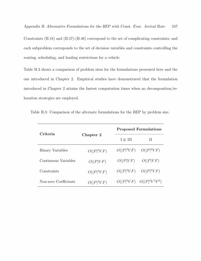
Appendix B. Alternative Formulations for the BEP with Const. Evac. Arrival Rate 247
Constraints (B.18) and (B.47)-(B.48) correspond to the set of complicating constraints; and
each subproblem corresponds to the set of decision variables and constraints controlling the
routing, scheduling, and loading restrictions for a vehicle.
Table B.3 shows a comparison of problem sizes for the formulations presented here and the
one introduced in Chapter 2. Empirical studies have demonstrated that the formulation
introduced in Chapter 2 attains the fastest computation times when no decomposition/re-
laxation strategies are employed.
Table B.3: Comparison of the alternate formulations for the BEP by problem size.
Criteria Chapter 2
Proposed Formulations
I & III II
Binary Variables O(|P |2V F ) O(|P |2V F ) O(|P |2V F )
Continuous Variables O(|P |V F ) O(|P |V F ) O(|P |V F )
Constraints O(|P |2V F ) O(|P |2V F ) O(|P |2V F )
Non-zero Coefficients O(|P |2V F ) O(|P |2V F ) O(|P |2V 2F 2)

Appendix C
Numerical Examples of the Original
and Modified Ritter (1967)
Relaxation Algorithms
248

Appendix C. Numerical Examples of the Ritter (1967) Relaxation Algorithms 249
C.1 Example Problem
This appendix illustrates the differences between the original and the modified Ritter (1967)
Relaxation Algorithms. Consider the following, bordered (or arrowhead) structure, linear
programming problem. Observe that the problem is already in standard form and that all
decision variables are non-negative.
Minimize x1 + 12x2 + 3
4x3 + 3
8x4 − x5 − x6 + 3
2x7
Subject to 2x1 + x3 + x7 + 2x8 = 11
x2 + 2 x3 − x7 + x8 = 8
+ 13x4 + 2
3x6 + x7 = 5
x5 + 3 x6 + 12x7 − x8 = 9
12x1 + x2 + x4 + x5 − x7 + x8 = 8
x1 , x2 , x3 , x4 , x5 , x6 , x7 , x8 ≥ 0
Let x7 and x8 be complicating decision variables, and let the last structural constraint be
the only complicating constraint. Consequently, the problem has two subproblems: the first
involving x1, x2, and x3, and the second, x4, x5, and x6. First, the problem is solved via
the original Ritter (1967) Relaxation Algorithm.
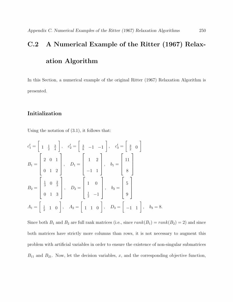
Appendix C. Numerical Examples of the Ritter (1967) Relaxation Algorithms 250
C.2 A Numerical Example of the Ritter (1967) Relax-
ation Algorithm
In this Section, a numerical example of the original Ritter (1967) Relaxation Algorithm is
presented.
Initialization
Using the notation of (3.1), it follows that:
ct1 =
[1 1
234
], ct2 =
[38−1 −1
], ct3 =
[32
0
]
B1 =
2 0 1
0 1 2
, D1 =
1 2
−1 1
, b1 =
11
8
B2 =
13
0 23
0 1 3
, D2 =
1 0
12−1
, b2 =
5
9
A1 =
[12
1 0
], A2 =
[1 1 0
], D3 =
[−1 1
], b3 = 8.
Since both B1 and B2 are full rank matrices (i.e., since rank(B1) = rank(B2) = 2) and since
both matrices have strictly more columns than rows, it is not necessary to augment this
problem with artificial variables in order to ensure the existence of non-singular submatrices
B11 and B21. Now, let the decision variables, x, and the corresponding objective function,
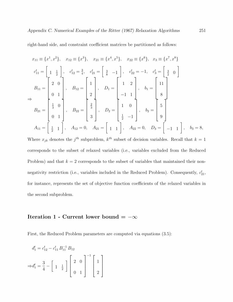
Appendix C. Numerical Examples of the Ritter (1967) Relaxation Algorithms 251
right-hand side, and constraint coefficient matrices be partitioned as follows:
x11 ≡ {x1, x2}, x12 ≡ {x3}, x21 ≡ {x4, x5}, x22 ≡ {x6}, x3 ≡ {x7, x8}
⇒
ct11 =
[1 1
2
], ct12 = 3
4, ct21 =
[38−1
], ct22 = −1, ct3 =
[32
0
]
B11 =
2 0
0 1
, B12 =
1
2
, D1 =
1 2
−1 1
, b1 =
11
8
B21 =
13
0
0 1
, B22 =
23
3
, D2 =
1 0
12−1
, b2 =
5
9
A11 =
[12
1
], A12 = 0, A21 =
[1 1
], A22 = 0, D3 =
[−1 1
], b3 = 8,
Where xjk denotes the jth subproblem, kth subset of decision variables. Recall that k = 1
corresponds to the subset of relaxed variables (i.e., variables excluded from the Reduced
Problem) and that k = 2 corresponds to the subset of variables that maintained their non-
negativity restriction (i.e., variables included in the Reduced Problem). Consequently, ct21,
for instance, represents the set of objective function coefficients of the relaxed variables in
the second subproblem.
Iteration 1 - Current lower bound = −∞
First, the Reduced Problem parameters are computed via equations (3.5):
dt1 = ct12 − ct11B−111 B12
⇒dt1 =3
4−[
1 12
]
2 0
0 1
−1
1
2
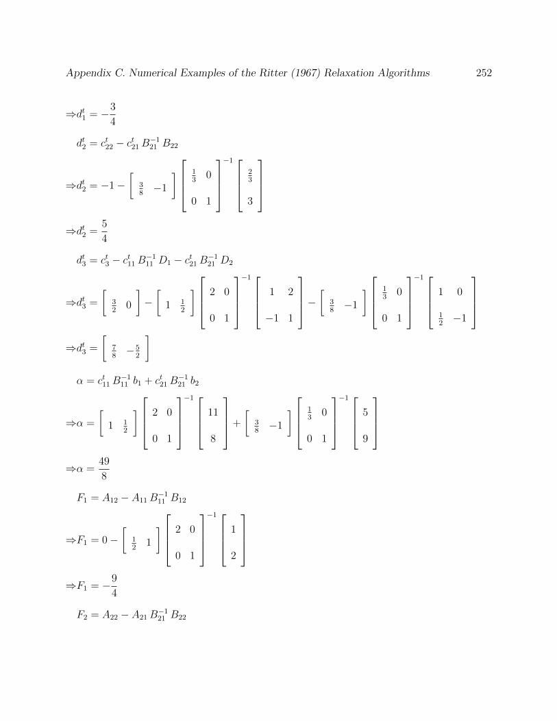
Appendix C. Numerical Examples of the Ritter (1967) Relaxation Algorithms 252
⇒dt1 = −3
4
dt2 = ct22 − ct21B−121 B22
⇒dt2 = −1−[
38−1
]
13
0
0 1
−1
23
3
⇒dt2 =5
4
dt3 = ct3 − ct11B−111 D1 − ct21B
−121 D2
⇒dt3 =
[32
0
]−[
1 12
]
2 0
0 1
−1
1 2
−1 1
−
[38−1
]
13
0
0 1
−1
1 0
12−1
⇒dt3 =
[78−5
2
]
α = ct11B−111 b1 + ct21B
−121 b2
⇒α =
[1 1
2
]
2 0
0 1
−1
11
8
+
[38−1
]
13
0
0 1
−1
5
9
⇒α =49
8
F1 = A12 − A11B−111 B12
⇒F1 = 0−[
12
1
]
2 0
0 1
−1
1
2
⇒F1 = −9
4
F2 = A22 − A21B−121 B22
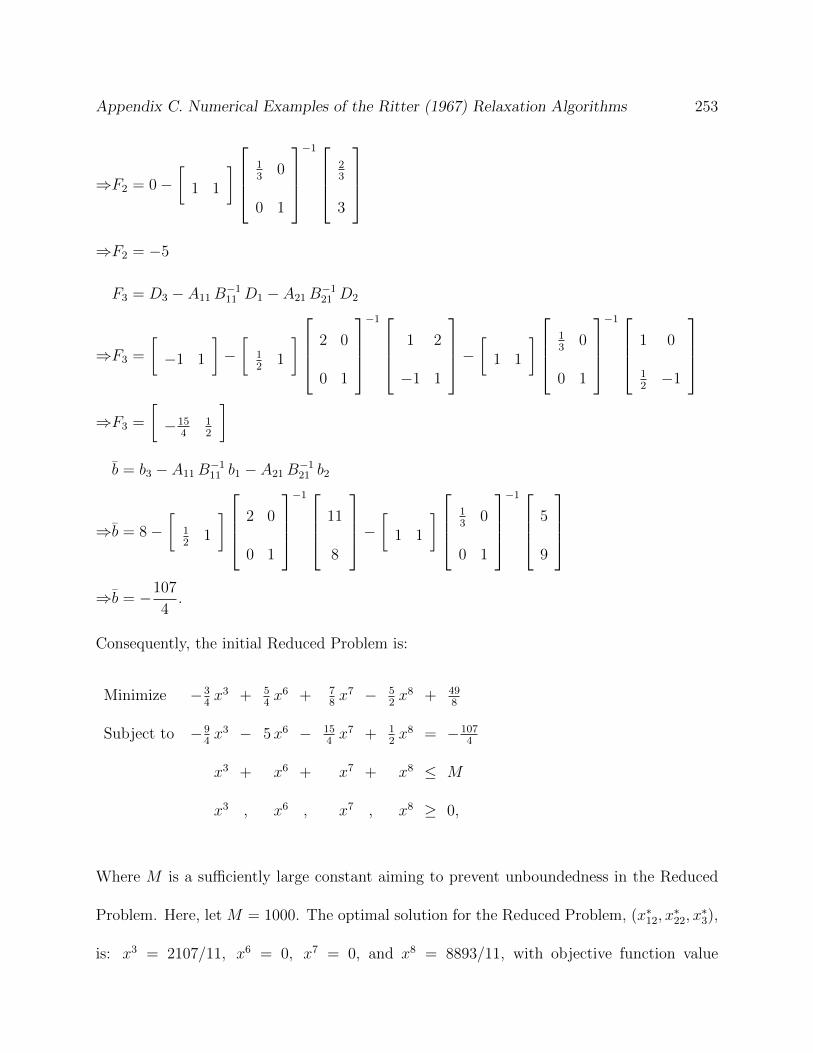
Appendix C. Numerical Examples of the Ritter (1967) Relaxation Algorithms 253
⇒F2 = 0−[
1 1
]
13
0
0 1
−1
23
3
⇒F2 = −5
F3 = D3 − A11B−111 D1 − A21B
−121 D2
⇒F3 =
[−1 1
]−[
12
1
]
2 0
0 1
−1
1 2
−1 1
−
[1 1
]
13
0
0 1
−1
1 0
12−1
⇒F3 =
[−15
412
]
b = b3 − A11B−111 b1 − A21B
−121 b2
⇒b = 8−[
12
1
]
2 0
0 1
−1
11
8
−
[1 1
]
13
0
0 1
−1
5
9
⇒b = −107
4.
Consequently, the initial Reduced Problem is:
Minimize −34x3 + 5
4x6 + 7
8x7 − 5
2x8 + 49
8
Subject to −94x3 − 5x6 − 15
4x7 + 1
2x8 = −107
4
x3 + x6 + x7 + x8 ≤ M
x3 , x6 , x7 , x8 ≥ 0,
Where M is a sufficiently large constant aiming to prevent unboundedness in the Reduced
Problem. Here, let M = 1000. The optimal solution for the Reduced Problem, (x∗12, x∗22, x
∗3),
is: x3 = 2107/11, x6 = 0, x7 = 0, and x8 = 8893/11, with objective function value

Appendix C. Numerical Examples of the Ritter (1967) Relaxation Algorithms 254
−189963/88 ≈ −2158.670. Such objective function value corresponds to the new lower bound
on the objective function value for the original (non-relaxed) problem. The corresponding
optimal x∗11 and x∗21 decision variables are attained via (3.3):
x∗11 = B−111 b1 −B−1
11 B12 x∗12 −B−1
11 D1 x∗3
⇒x∗11 =
2 0
0 1
−1
11
8
−
1
2
(
2107
11
)−
1 2
−1 1
0
889311
=
−9886
11
−1301911
⇒x1 = −9886
11, x2 = −13019
11
x∗21 = B−121 b2 −B−1
21 B22 x∗22 −B−1
21 D2 x∗3
⇒x∗21 =
13
0
0 1
−1
5
9
−
23
3
(0)−
1 0
12−1
0
889311
=
15
899211
⇒x4 = 15, x5 =8992
11.
Since both elements of set x11 are negative, a new iteration is needed. Observe that the
constraint used to prevent unboundedness in the Reduced Problem is binding.
Iteration 2 - Current lower bound = −2158.670
If the ith element of x∗11 is negative, if the jth element of x∗12 is positive, and if the ith row, jth
column of B−111 B12 6= 0, then those elements can be swapped without producing a singular
B11 submatrix. Currently, both elements of x∗11 are negative and the only element of x∗12 is
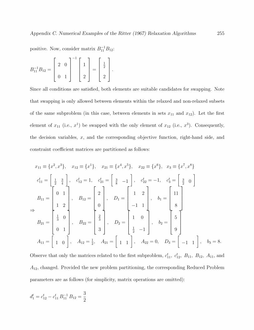
Appendix C. Numerical Examples of the Ritter (1967) Relaxation Algorithms 255
positive. Now, consider matrix B−111 B12:
B−111 B12 =
2 0
0 1
−1
1
2
=
12
2
.
Since all conditions are satisfied, both elements are suitable candidates for swapping. Note
that swapping is only allowed between elements within the relaxed and non-relaxed subsets
of the same subproblem (in this case, between elements in sets x11 and x12). Let the first
element of x11 (i.e., x1) be swapped with the only element of x12 (i.e., x3). Consequently,
the decision variables, x, and the corresponding objective function, right-hand side, and
constraint coefficient matrices are partitioned as follows:
x11 ≡ {x2, x3}, x12 ≡ {x1}, x21 ≡ {x4, x5}, x22 ≡ {x6}, x3 ≡ {x7, x8}
⇒
ct11 =
[12
34
], ct12 = 1, ct21 =
[38−1
], ct22 = −1, ct3 =
[32
0
]
B11 =
0 1
1 2
, B12 =
2
0
, D1 =
1 2
−1 1
, b1 =
11
8
B21 =
13
0
0 1
, B22 =
23
3
, D2 =
1 0
12−1
, b2 =
5
9
A11 =
[1 0
], A12 = 1
2, A21 =
[1 1
], A22 = 0, D3 =
[−1 1
], b3 = 8.
Observe that only the matrices related to the first subproblem, ct11, ct12, B11, B12, A11, and
A12, changed. Provided the new problem partitioning, the corresponding Reduced Problem
parameters are as follows (for simplicity, matrix operations are omitted):
dt1 = ct12 − ct11B−111 B12 =
3
2
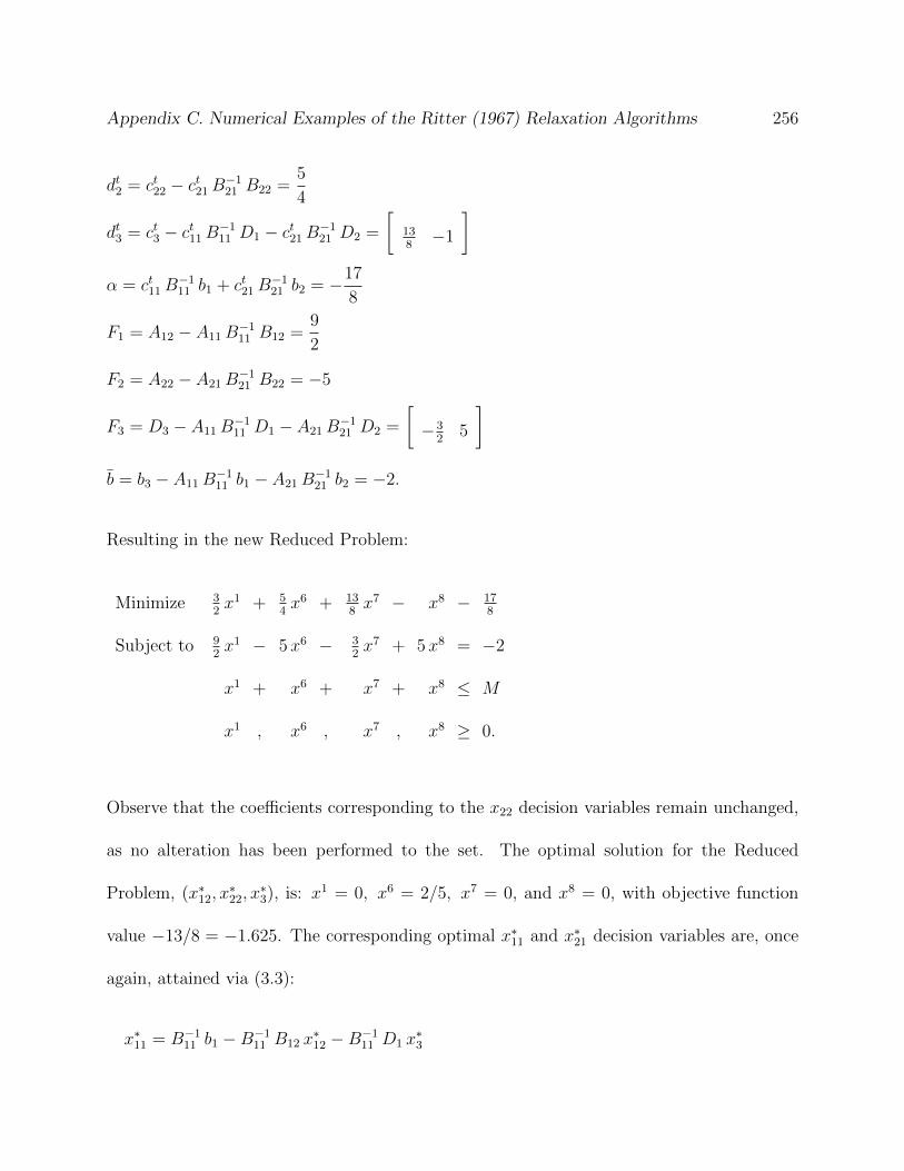
Appendix C. Numerical Examples of the Ritter (1967) Relaxation Algorithms 256
dt2 = ct22 − ct21B−121 B22 =
5
4
dt3 = ct3 − ct11B−111 D1 − ct21B
−121 D2 =
[138−1
]
α = ct11B−111 b1 + ct21B
−121 b2 = −17
8
F1 = A12 − A11B−111 B12 =
9
2
F2 = A22 − A21B−121 B22 = −5
F3 = D3 − A11B−111 D1 − A21B
−121 D2 =
[−3
25
]
b = b3 − A11B−111 b1 − A21B
−121 b2 = −2.
Resulting in the new Reduced Problem:
Minimize 32x1 + 5
4x6 + 13
8x7 − x8 − 17
8
Subject to 92x1 − 5x6 − 3
2x7 + 5x8 = −2
x1 + x6 + x7 + x8 ≤ M
x1 , x6 , x7 , x8 ≥ 0.
Observe that the coefficients corresponding to the x22 decision variables remain unchanged,
as no alteration has been performed to the set. The optimal solution for the Reduced
Problem, (x∗12, x∗22, x
∗3), is: x1 = 0, x6 = 2/5, x7 = 0, and x8 = 0, with objective function
value −13/8 = −1.625. The corresponding optimal x∗11 and x∗21 decision variables are, once
again, attained via (3.3):
x∗11 = B−111 b1 −B−1
11 B12 x∗12 −B−1
11 D1 x∗3
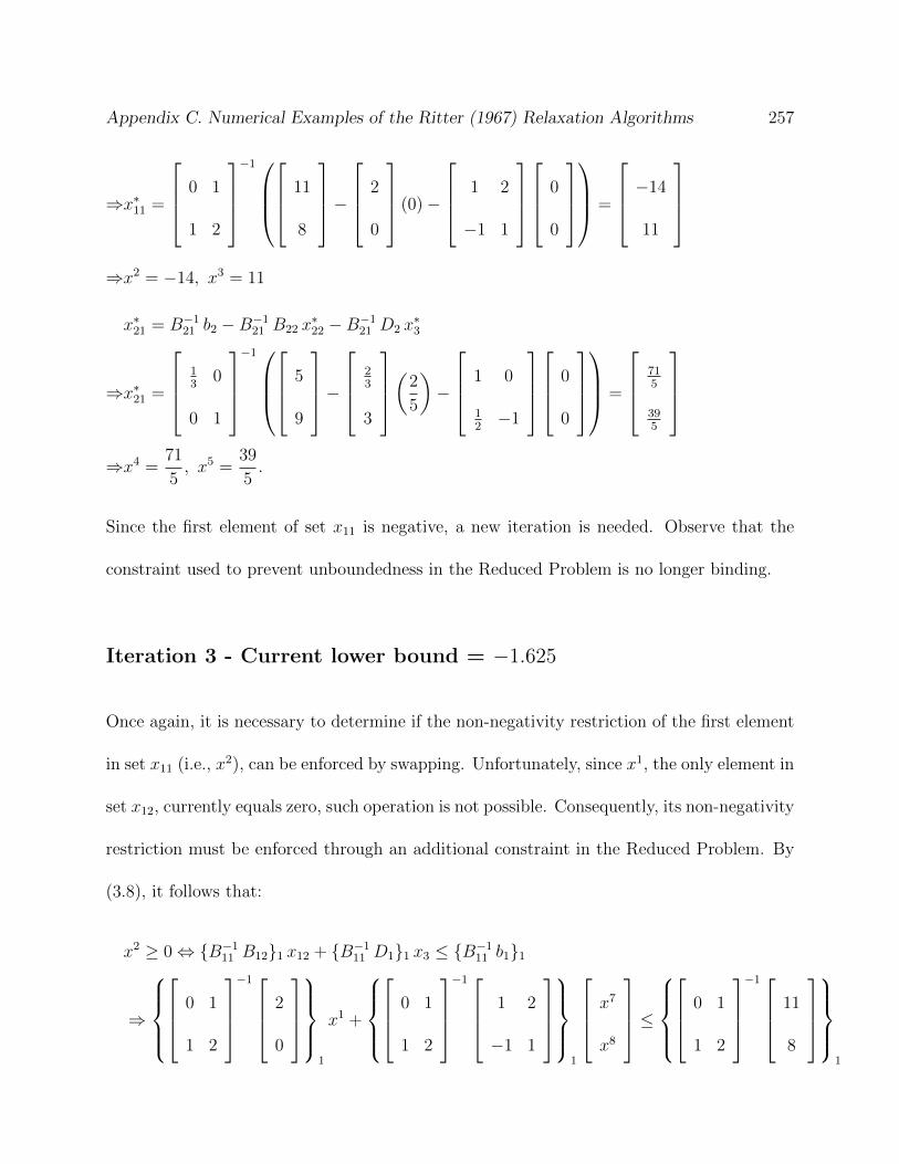
Appendix C. Numerical Examples of the Ritter (1967) Relaxation Algorithms 257
⇒x∗11 =
0 1
1 2
−1
11
8
−
2
0
(0)−
1 2
−1 1
0
0
=
−14
11
⇒x2 = −14, x3 = 11
x∗21 = B−121 b2 −B−1
21 B22 x∗22 −B−1
21 D2 x∗3
⇒x∗21 =
13
0
0 1
−1
5
9
−
23
3
(
2
5
)−
1 0
12−1
0
0
=
715
395
⇒x4 =71
5, x5 =
39
5.
Since the first element of set x11 is negative, a new iteration is needed. Observe that the
constraint used to prevent unboundedness in the Reduced Problem is no longer binding.
Iteration 3 - Current lower bound = −1.625
Once again, it is necessary to determine if the non-negativity restriction of the first element
in set x11 (i.e., x2), can be enforced by swapping. Unfortunately, since x1, the only element in
set x12, currently equals zero, such operation is not possible. Consequently, its non-negativity
restriction must be enforced through an additional constraint in the Reduced Problem. By
(3.8), it follows that:
x2 ≥ 0⇔ {B−111 B12}1 x12 + {B−1
11 D1}1 x3 ≤ {B−111 b1}1
⇒
0 1
1 2
−1
2
0
1
x1 +
0 1
1 2
−1
1 2
−1 1
1
x7
x8
≤
0 1
1 2
−1
11
8
1
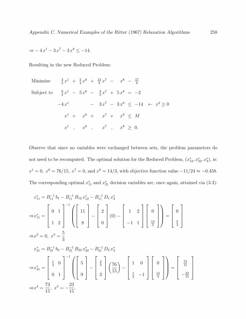
Appendix C. Numerical Examples of the Ritter (1967) Relaxation Algorithms 258
⇒− 4x1 − 3x7 − 3x8 ≤ −14.
Resulting in the new Reduced Problem:
Minimize 32x1 + 5
4x6 + 13
8x7 − x8 − 17
8
Subject to 92x1 − 5x6 − 3
2x7 + 5x8 = −2
−4x1 − 3x7 − 3x8 ≤ −14 ← x2 ≥ 0
x1 + x6 + x7 + x8 ≤ M
x1 , x6 , x7 , x8 ≥ 0.
Observe that since no variables were exchanged between sets, the problem parameters do
not need to be recomputed. The optimal solution for the Reduced Problem, (x∗12, x∗22, x
∗3), is:
x1 = 0, x6 = 76/15, x7 = 0, and x8 = 14/3, with objective function value −11/24 ≈ −0.458.
The corresponding optimal x∗11 and x∗21 decision variables are, once again, attained via (3.3):
x∗11 = B−111 b1 −B−1
11 B12 x∗12 −B−1
11 D1 x∗3
⇒x∗11 =
0 1
1 2
−1
11
8
−
2
0
(0)−
1 2
−1 1
0
143
=
0
53
⇒x2 = 0, x3 =5
3
x∗21 = B−121 b2 −B−1
21 B22 x∗22 −B−1
21 D2 x∗3
⇒x∗21 =
13
0
0 1
−1
5
9
−
23
3
(
76
15
)−
1 0
12−1
0
143
=
7315
−2315
⇒x4 =73
15, x5 = −23
15.
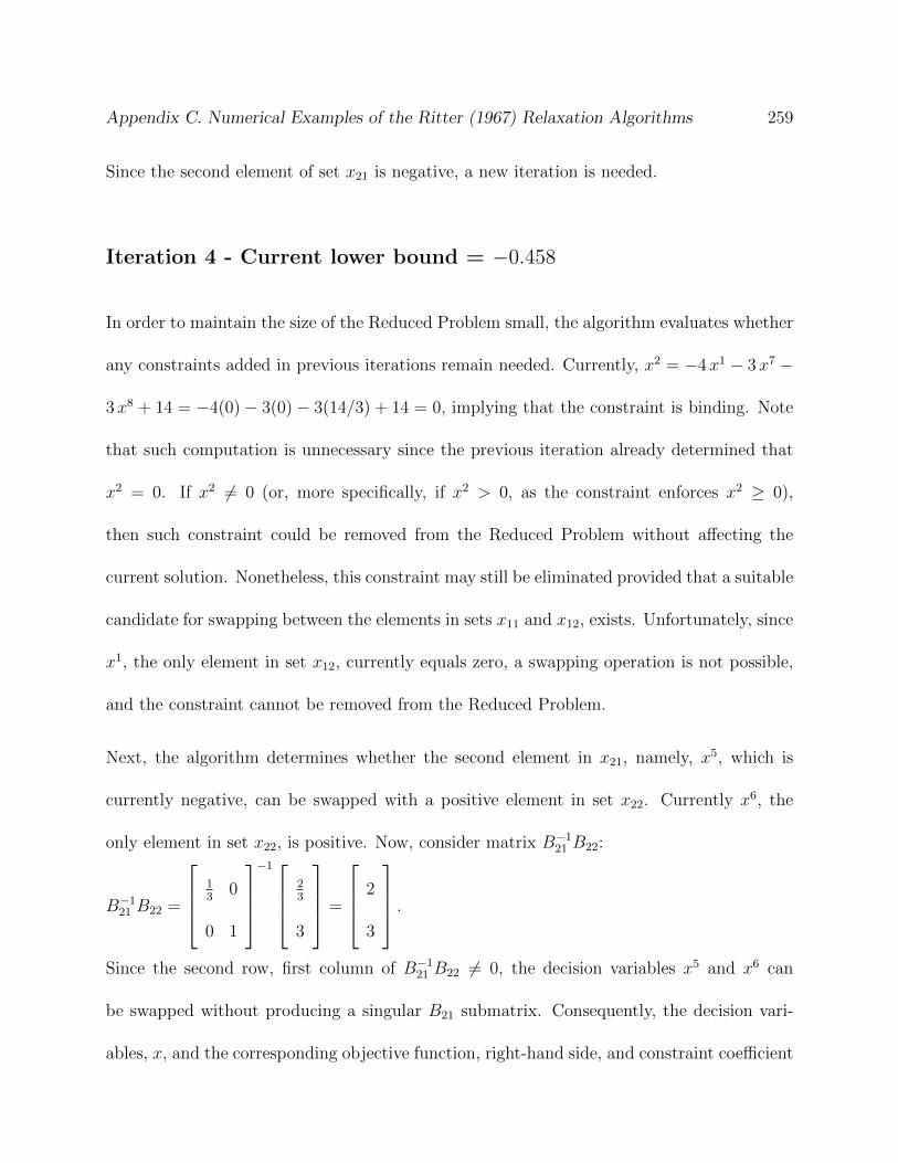
Appendix C. Numerical Examples of the Ritter (1967) Relaxation Algorithms 259
Since the second element of set x21 is negative, a new iteration is needed.
Iteration 4 - Current lower bound = −0.458
In order to maintain the size of the Reduced Problem small, the algorithm evaluates whether
any constraints added in previous iterations remain needed. Currently, x2 = −4x1 − 3x7 −
3x8 + 14 = −4(0)− 3(0)− 3(14/3) + 14 = 0, implying that the constraint is binding. Note
that such computation is unnecessary since the previous iteration already determined that
x2 = 0. If x2 6= 0 (or, more specifically, if x2 > 0, as the constraint enforces x2 ≥ 0),
then such constraint could be removed from the Reduced Problem without affecting the
current solution. Nonetheless, this constraint may still be eliminated provided that a suitable
candidate for swapping between the elements in sets x11 and x12, exists. Unfortunately, since
x1, the only element in set x12, currently equals zero, a swapping operation is not possible,
and the constraint cannot be removed from the Reduced Problem.
Next, the algorithm determines whether the second element in x21, namely, x5, which is
currently negative, can be swapped with a positive element in set x22. Currently x6, the
only element in set x22, is positive. Now, consider matrix B−121 B22:
B−121 B22 =
13
0
0 1
−1
23
3
=
2
3
.
Since the second row, first column of B−121 B22 6= 0, the decision variables x5 and x6 can
be swapped without producing a singular B21 submatrix. Consequently, the decision vari-
ables, x, and the corresponding objective function, right-hand side, and constraint coefficient

Appendix C. Numerical Examples of the Ritter (1967) Relaxation Algorithms 260
matrices are partitioned as follows:
x11 ≡ {x2, x3}, x12 ≡ {x1}, x21 ≡ {x4, x6}, x22 ≡ {x5}, x3 ≡ {x7, x8}
⇒
ct11 =
[12
34
], ct12 = 1, ct21 =
[38−1
], ct22 = −1, ct3 =
[32
0
]
B11 =
0 1
1 2
, B12 =
2
0
, D1 =
1 2
−1 1
, b1 =
11
8
B21 =
13
23
0 3
, B22 =
0
1
, D2 =
1 0
12−1
, b2 =
5
9
A11 =
[1 0
], A12 = 1
2, A21 =
[1 0
], A22 = 1, D3 =
[−1 1
], b3 = 8.
Once again, observe that only the matrices related to the second subproblem,
ct21, ct22, B21, B22, A21, and A22 changed. Provided the new problem partitioning, the
corresponding Reduced Problem parameters are as follows (for simplicity, matrix operations
are omitted):
dt1 = ct12 − ct11B−111 B12 =
3
2
dt2 = ct22 − ct21B−121 B22 = − 5
12
dt3 = ct3 − ct11B−111 D1 − ct21B
−121 D2 =
[1712− 7
12
]
α = ct11B−111 b1 + ct21B
−121 b2 =
13
8
F1 = A12 − A11B−111 B12 =
9
2
F2 = A22 − A21B−121 B22 =
5
3
F3 = D3 − A11B−111 D1 − A21B
−121 D2 =
[−2
3103
]
b = b3 − A11B−111 b1 − A21B
−121 b2 = 13.
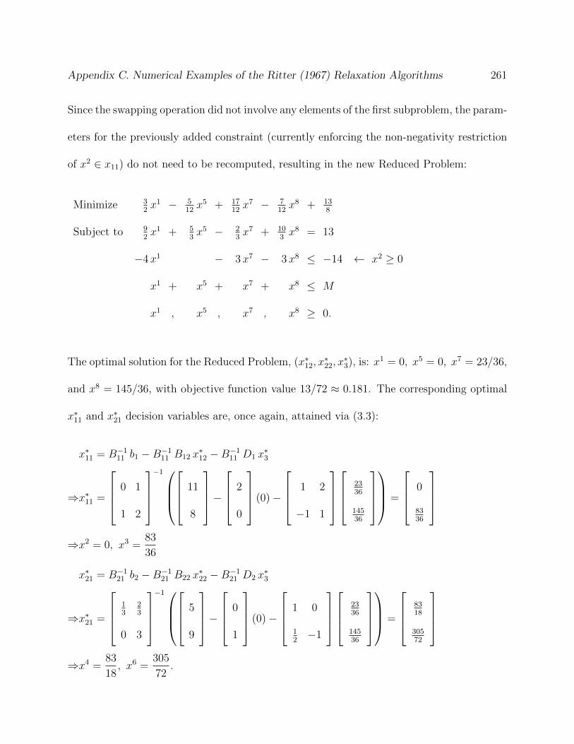
Appendix C. Numerical Examples of the Ritter (1967) Relaxation Algorithms 261
Since the swapping operation did not involve any elements of the first subproblem, the param-
eters for the previously added constraint (currently enforcing the non-negativity restriction
of x2 ∈ x11) do not need to be recomputed, resulting in the new Reduced Problem:
Minimize 32x1 − 5
12x5 + 17
12x7 − 7
12x8 + 13
8
Subject to 92x1 + 5
3x5 − 2
3x7 + 10
3x8 = 13
−4x1 − 3x7 − 3x8 ≤ −14 ← x2 ≥ 0
x1 + x5 + x7 + x8 ≤ M
x1 , x5 , x7 , x8 ≥ 0.
The optimal solution for the Reduced Problem, (x∗12, x∗22, x
∗3), is: x1 = 0, x5 = 0, x7 = 23/36,
and x8 = 145/36, with objective function value 13/72 ≈ 0.181. The corresponding optimal
x∗11 and x∗21 decision variables are, once again, attained via (3.3):
x∗11 = B−111 b1 −B−1
11 B12 x∗12 −B−1
11 D1 x∗3
⇒x∗11 =
0 1
1 2
−1
11
8
−
2
0
(0)−
1 2
−1 1
2336
14536
=
0
8336
⇒x2 = 0, x3 =83
36
x∗21 = B−121 b2 −B−1
21 B22 x∗22 −B−1
21 D2 x∗3
⇒x∗21 =
13
23
0 3
−1
5
9
−
0
1
(0)−
1 0
12−1
2336
14536
=
8318
30572
⇒x4 =83
18, x6 =
305
72.

Appendix C. Numerical Examples of the Ritter (1967) Relaxation Algorithms 262
Since all elements of sets x11 and x21 are non-negative, the algorithm terminates with optimal
solution: x1 = 0, x2 = 0, x3 = 83/36, x4 = 83/18, x5 = 0, x6 = 305/72, x7 = 23/36, and
x8 = 145/36, and objective function value of 13/72 ≈ 0.181.
Next, it is shown that the original problem can be solved without the swapping operation.
Although the operation helps maintain the size of the Reduced Problem small, restricting
the number of constraints enforcing the non-negativity restriction of the relaxed variables
also demands considerably more computations, thus leading to numerical instabilities.
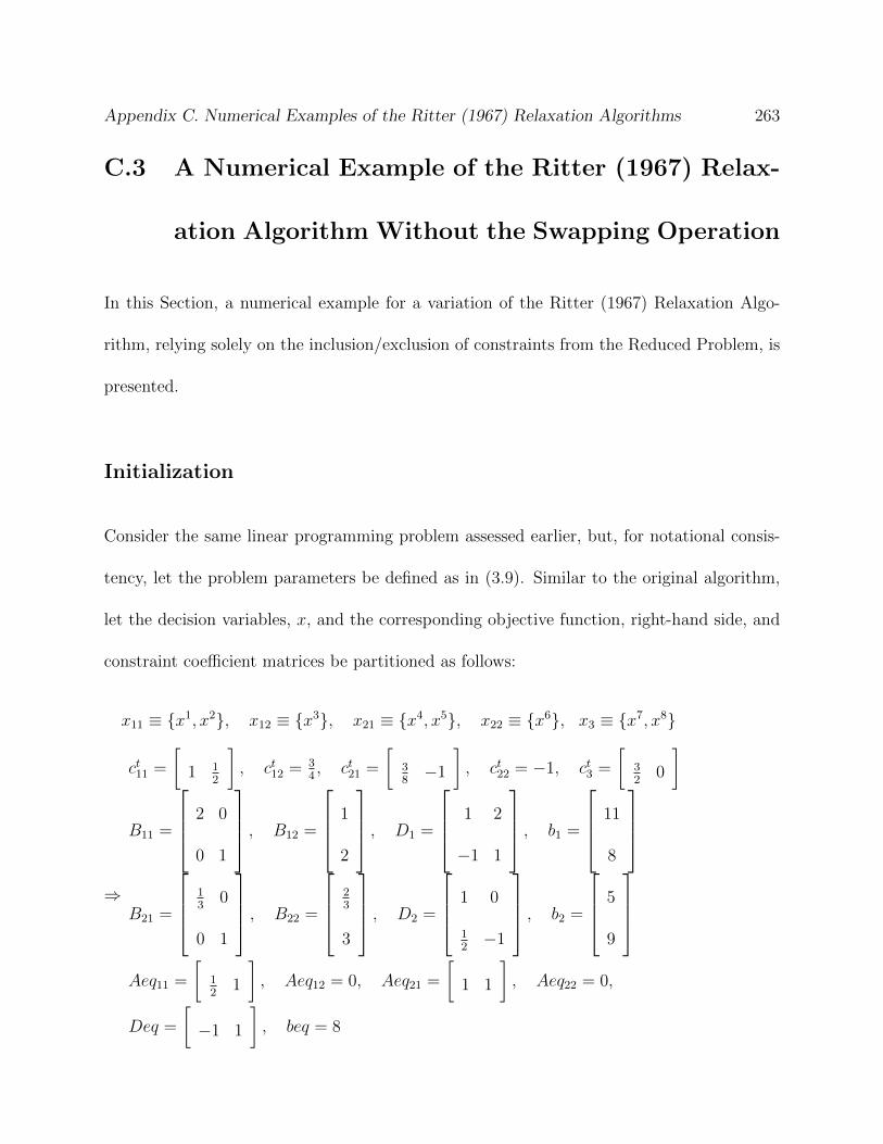
Appendix C. Numerical Examples of the Ritter (1967) Relaxation Algorithms 263
C.3 A Numerical Example of the Ritter (1967) Relax-
ation Algorithm Without the Swapping Operation
In this Section, a numerical example for a variation of the Ritter (1967) Relaxation Algo-
rithm, relying solely on the inclusion/exclusion of constraints from the Reduced Problem, is
presented.
Initialization
Consider the same linear programming problem assessed earlier, but, for notational consis-
tency, let the problem parameters be defined as in (3.9). Similar to the original algorithm,
let the decision variables, x, and the corresponding objective function, right-hand side, and
constraint coefficient matrices be partitioned as follows:
x11 ≡ {x1, x2}, x12 ≡ {x3}, x21 ≡ {x4, x5}, x22 ≡ {x6}, x3 ≡ {x7, x8}
⇒
ct11 =
[1 1
2
], ct12 = 3
4, ct21 =
[38−1
], ct22 = −1, ct3 =
[32
0
]
B11 =
2 0
0 1
, B12 =
1
2
, D1 =
1 2
−1 1
, b1 =
11
8
B21 =
13
0
0 1
, B22 =
23
3
, D2 =
1 0
12−1
, b2 =
5
9
Aeq11 =
[12
1
], Aeq12 = 0, Aeq21 =
[1 1
], Aeq22 = 0,
Deq =
[−1 1
], beq = 8

Appendix C. Numerical Examples of the Ritter (1967) Relaxation Algorithms 264
Since the algorithm does not rely on the swapping operation, such problem parameters
remain unchanged throughout its execution. Now, let the following parameters, computed
via Equations (3.10), be defined. Such constants will be reused throughout the execution of
the algorithm:
B1 = B−111 B12 =
2 0
0 1
−1
1
2
=
12
2
B2 = B−121 B22 =
13
0
0 1
−1
23
3
=
2
3
D1 = B−111 D1 =
2 0
0 1
−1
1 2
−1 1
=
12
1
−1 1
D2 = B−121 D2 =
13
0
0 1
−1
1 0
12−1
=
3 0
12−1
b1 = B−111 b1 =
2 0
0 1
−1
11
8
=
112
8
b2 = B−121 b2 =
13
0
0 1
−1
5
9
=
15
9
.
Iteration 1 - Current lower bound = −∞
First, the Reduced Problem parameters are computed via (3.13). Except for a few notational
differences, these computations are identical to the ones performed on the first iteration of
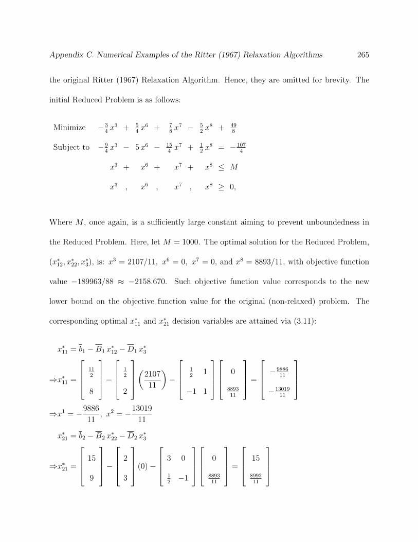
Appendix C. Numerical Examples of the Ritter (1967) Relaxation Algorithms 265
the original Ritter (1967) Relaxation Algorithm. Hence, they are omitted for brevity. The
initial Reduced Problem is as follows:
Minimize −34x3 + 5
4x6 + 7
8x7 − 5
2x8 + 49
8
Subject to −94x3 − 5x6 − 15
4x7 + 1
2x8 = −107
4
x3 + x6 + x7 + x8 ≤ M
x3 , x6 , x7 , x8 ≥ 0,
Where M , once again, is a sufficiently large constant aiming to prevent unboundedness in
the Reduced Problem. Here, let M = 1000. The optimal solution for the Reduced Problem,
(x∗12, x∗22, x
∗3), is: x3 = 2107/11, x6 = 0, x7 = 0, and x8 = 8893/11, with objective function
value −189963/88 ≈ −2158.670. Such objective function value corresponds to the new
lower bound on the objective function value for the original (non-relaxed) problem. The
corresponding optimal x∗11 and x∗21 decision variables are attained via (3.11):
x∗11 = b1 −B1 x∗12 −D1 x
∗3
⇒x∗11 =
112
8
−
12
2
(
2107
11
)−
12
1
−1 1
0
889311
=
−9886
11
−1301911
⇒x1 = −9886
11, x2 = −13019
11
x∗21 = b2 −B2 x∗22 −D2 x
∗3
⇒x∗21 =
15
9
−
2
3
(0)−
3 0
12−1
0
889311
=
15
899211

Appendix C. Numerical Examples of the Ritter (1967) Relaxation Algorithms 266
⇒x4 = 15, x5 =8992
11.
Since both elements of set x11 are negative, a new iteration is needed. Observe that the
constraint used to prevent unboundedness in the Reduced Problem is binding.
Iteration 2 - Current lower bound = −2158.670
In the original algorithm, a test is performed to determine whether any variables can be
swapped between the relaxed and non-relaxed sets. Here, however, such operation is not
performed. Instead, the non-negativity restriction on violated decision variables is enforced
by new constraints added to the Reduced Problem. Since added constraints may also affect
the current solution of alternative decision variables (unintentionally enforcing their non-
negativity restriction), as a rule-of-thumb, let only the restriction on the most violated
decision variable within each subproblem be enforced, in this case, x2. Now, by (3.12):
x2 ≥ 0⇔{B1}2 x12 + {D1}2 x3 ≤ {b1}2
⇒
12
2
2
x3 +
12
1
−1 1
2
x7
x8
≤
112
8
2
⇒2x3 − x7 + x8 ≤ 8.
Resulting in the new Reduced Problem:
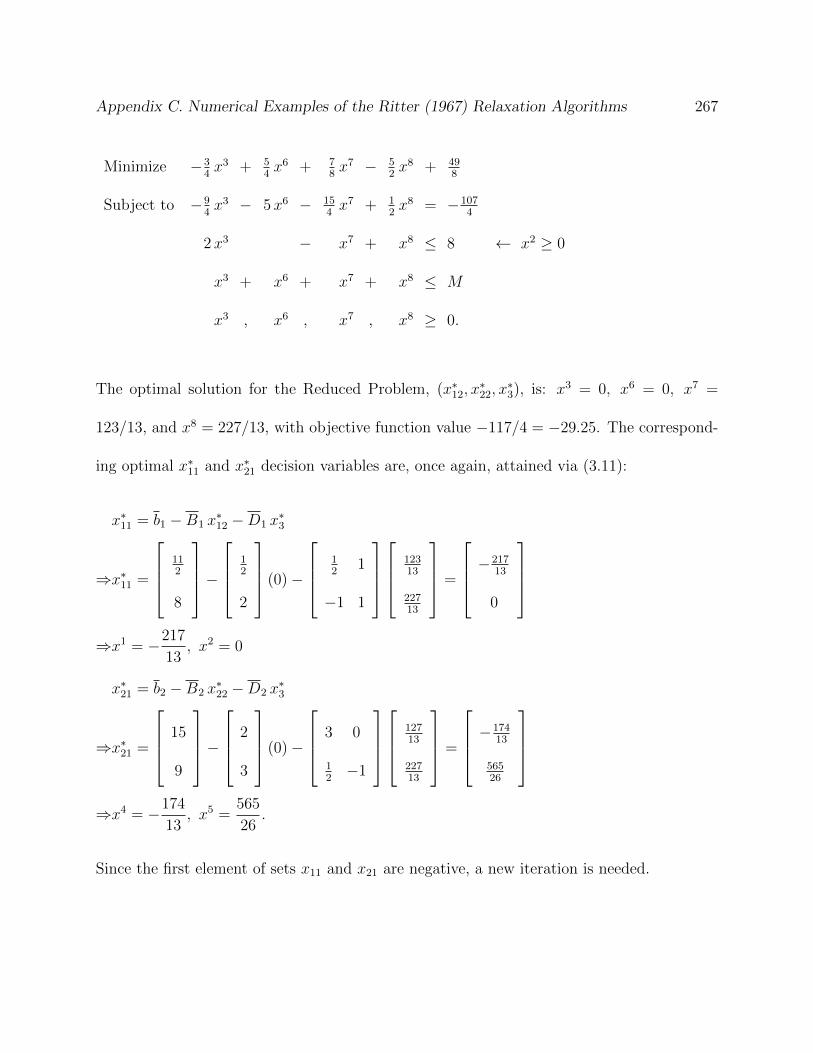
Appendix C. Numerical Examples of the Ritter (1967) Relaxation Algorithms 267
Minimize −34x3 + 5
4x6 + 7
8x7 − 5
2x8 + 49
8
Subject to −94x3 − 5x6 − 15
4x7 + 1
2x8 = −107
4
2x3 − x7 + x8 ≤ 8 ← x2 ≥ 0
x3 + x6 + x7 + x8 ≤ M
x3 , x6 , x7 , x8 ≥ 0.
The optimal solution for the Reduced Problem, (x∗12, x∗22, x
∗3), is: x3 = 0, x6 = 0, x7 =
123/13, and x8 = 227/13, with objective function value −117/4 = −29.25. The correspond-
ing optimal x∗11 and x∗21 decision variables are, once again, attained via (3.11):
x∗11 = b1 −B1 x∗12 −D1 x
∗3
⇒x∗11 =
112
8
−
12
2
(0)−
12
1
−1 1
12313
22713
=
−217
13
0
⇒x1 = −217
13, x2 = 0
x∗21 = b2 −B2 x∗22 −D2 x
∗3
⇒x∗21 =
15
9
−
2
3
(0)−
3 0
12−1
12713
22713
=
−174
13
56526
⇒x4 = −174
13, x5 =
565
26.
Since the first element of sets x11 and x21 are negative, a new iteration is needed.

Appendix C. Numerical Examples of the Ritter (1967) Relaxation Algorithms 268
Iteration 3 - Current lower bound = −29.25
Now, in the original Ritter (1967) Relaxation Algorithm, previously added constraints can
be removed from the Reduced Problem if they are not binding or if they are binding but
a suitable candidate for swapping exists. Here, however, constraints are only eliminated
provided they are redundant. Consequently, the restriction x2 ≥ 0 cannot be removed from
the Reduced Problem.
Next, the constraints enforcing the non-negativity restriction on the first element of sets x11
and x21 (i.e., x1 and x4, respectively) are generated and added to the Reduced Problem.
Once again, by (3.12):
x1 ≥ 0⇔{B1}1 x12 + {D1}1 x3 ≤ {b1}1
⇒
12
2
1
x3 +
12
1
−1 1
1
x7
x8
≤
112
8
1
⇒1
2x3 +
1
2x7 + x8 ≤ 11
2
x4 ≥ 0⇔{B2}1 x22 + {D2}1 x3 ≤ {b2}1
⇒
2
3
1
x6 +
3 0
12−1
1
x7
x8
≤
15
9
1
⇒2x6 + 3x7 ≤ 15.
Resulting in the new Reduced Problem:
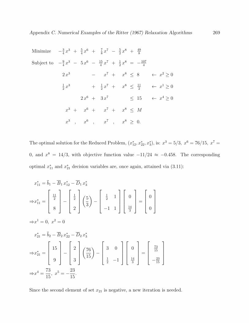
Appendix C. Numerical Examples of the Ritter (1967) Relaxation Algorithms 269
Minimize −34x3 + 5
4x6 + 7
8x7 − 5
2x8 + 49
8
Subject to −94x3 − 5x6 − 15
4x7 + 1
2x8 = −107
4
2x3 − x7 + x8 ≤ 8 ← x2 ≥ 0
12x3 + 1
2x7 + x8 ≤ 11
2← x1 ≥ 0
2x6 + 3x7 ≤ 15 ← x4 ≥ 0
x3 + x6 + x7 + x8 ≤ M
x3 , x6 , x7 , x8 ≥ 0.
The optimal solution for the Reduced Problem, (x∗12, x∗22, x
∗3), is: x3 = 5/3, x6 = 76/15, x7 =
0, and x8 = 14/3, with objective function value −11/24 ≈ −0.458. The corresponding
optimal x∗11 and x∗21 decision variables are, once again, attained via (3.11):
x∗11 = b1 −B1 x∗12 −D1 x
∗3
⇒x∗11 =
112
8
−
12
2
(
5
3
)−
12
1
−1 1
0
143
=
0
0
⇒x1 = 0, x2 = 0
x∗21 = b2 −B2 x∗22 −D2 x
∗3
⇒x∗21 =
15
9
−
2
3
(
76
15
)−
3 0
12−1
0
143
=
7315
−2315
⇒x4 =73
15, x5 = −23
15.
Since the second element of set x21 is negative, a new iteration is needed.

Appendix C. Numerical Examples of the Ritter (1967) Relaxation Algorithms 270
Iteration 4 - Current lower bound = −0.458
While non-binding, the constraint enforcing the non-negativity restriction of the first element
of set x21 (i.e., x4) is maintained. Next, the constraint enforcing the non-negativity restriction
on the second element of set x21 (i.e., x5) is generated and added to the Reduced Problem.
Once again, by (3.12):
x5 ≥ 0⇔{B2}2 x22 + {D2}2 x3 ≤ {b2}2
⇒
2
3
2
x6 +
3 0
12−1
2
x7
x8
≤
15
9
2
⇒3x6 +1
2x7 − x8 ≤ 9.
Resulting in the new Reduced Problem:
Minimize −34x3 + 5
4x6 + 7
8x7 − 5
2x8 + 49
8
Subject to −94x3 − 5x6 − 15
4x7 + 1
2x8 = −107
4
2x3 − x7 + x8 ≤ 8 ← x2 ≥ 0
12x3 + 1
2x7 + x8 ≤ 11
2← x1 ≥ 0
2x6 + 3x7 ≤ 15 ← x4 ≥ 0
3x6 + 12x7 − x8 ≤ 9 ← x5 ≥ 0
x3 + x6 + x7 + x8 ≤ M
x3 , x6 , x7 , x8 ≥ 0.
The optimal solution for the Reduced Problem, (x∗12, x∗22, x
∗3), is: x3 = 83/36, x6 =
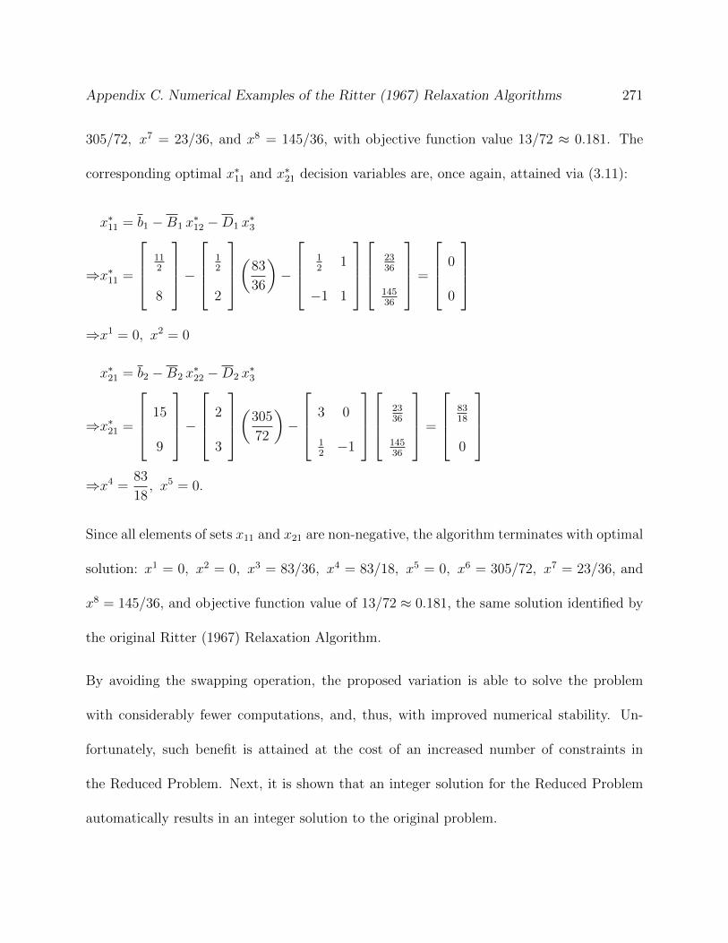
Appendix C. Numerical Examples of the Ritter (1967) Relaxation Algorithms 271
305/72, x7 = 23/36, and x8 = 145/36, with objective function value 13/72 ≈ 0.181. The
corresponding optimal x∗11 and x∗21 decision variables are, once again, attained via (3.11):
x∗11 = b1 −B1 x∗12 −D1 x
∗3
⇒x∗11 =
112
8
−
12
2
(
83
36
)−
12
1
−1 1
2336
14536
=
0
0
⇒x1 = 0, x2 = 0
x∗21 = b2 −B2 x∗22 −D2 x
∗3
⇒x∗21 =
15
9
−
2
3
(
305
72
)−
3 0
12−1
2336
14536
=
8318
0
⇒x4 =83
18, x5 = 0.
Since all elements of sets x11 and x21 are non-negative, the algorithm terminates with optimal
solution: x1 = 0, x2 = 0, x3 = 83/36, x4 = 83/18, x5 = 0, x6 = 305/72, x7 = 23/36, and
x8 = 145/36, and objective function value of 13/72 ≈ 0.181, the same solution identified by
the original Ritter (1967) Relaxation Algorithm.
By avoiding the swapping operation, the proposed variation is able to solve the problem
with considerably fewer computations, and, thus, with improved numerical stability. Un-
fortunately, such benefit is attained at the cost of an increased number of constraints in
the Reduced Problem. Next, it is shown that an integer solution for the Reduced Problem
automatically results in an integer solution to the original problem.

Appendix C. Numerical Examples of the Ritter (1967) Relaxation Algorithms 272
C.4 A Numerical, Integer Example of the Ritter
(1967) Relaxation Algorithm Without the Swap-
ping Operation
In this Section, a numerical, integer example of the Ritter (1967) Relaxation Algorithm,
relying solely on the inclusion/exclusion of constraints from the Reduced Problem, is pre-
sented.
Initialization
Consider the same problem assessed earlier, but, now, let x ∈ Z+, that is, let the problem
decision variables be non-negative integers. Once again, let the decision variables, x, and
the corresponding objective function, right-hand side, and constraint coefficient matrices be
partitioned as follows:
x11 ≡ {x1, x2}, x12 ≡ {x3}, x21 ≡ {x4, x5}, x22 ≡ {x6}, x3 ≡ {x7, x8}
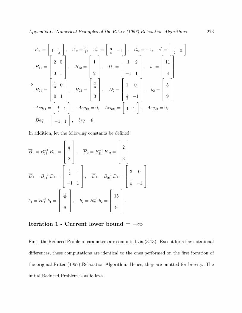
Appendix C. Numerical Examples of the Ritter (1967) Relaxation Algorithms 273
⇒
ct11 =
[1 1
2
], ct12 = 3
4, ct21 =
[38−1
], ct22 = −1, ct3 =
[32
0
]
B11 =
2 0
0 1
, B12 =
1
2
, D1 =
1 2
−1 1
, b1 =
11
8
B21 =
13
0
0 1
, B22 =
23
3
, D2 =
1 0
12−1
, b2 =
5
9
Aeq11 =
[12
1
], Aeq12 = 0, Aeq21 =
[1 1
], Aeq22 = 0,
Deq =
[−1 1
], beq = 8.
In addition, let the following constants be defined:
B1 = B−111 B12 =
12
2
, B2 = B−1
21 B22 =
2
3
D1 = B−111 D1 =
12
1
−1 1
, D2 = B−1
21 D2 =
3 0
12−1
b1 = B−111 b1 =
112
8
, b2 = B−1
21 b2 =
15
9
.
Iteration 1 - Current lower bound = −∞
First, the Reduced Problem parameters are computed via (3.13). Except for a few notational
differences, these computations are identical to the ones performed on the first iteration of
the original Ritter (1967) Relaxation Algorithm. Hence, they are omitted for brevity. The
initial Reduced Problem is as follows:
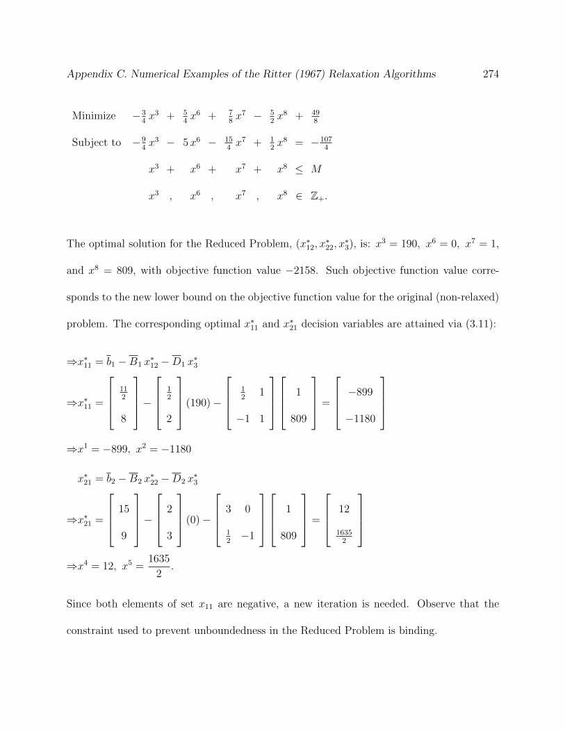
Appendix C. Numerical Examples of the Ritter (1967) Relaxation Algorithms 274
Minimize −34x3 + 5
4x6 + 7
8x7 − 5
2x8 + 49
8
Subject to −94x3 − 5x6 − 15
4x7 + 1
2x8 = −107
4
x3 + x6 + x7 + x8 ≤ M
x3 , x6 , x7 , x8 ∈ Z+.
The optimal solution for the Reduced Problem, (x∗12, x∗22, x
∗3), is: x3 = 190, x6 = 0, x7 = 1,
and x8 = 809, with objective function value −2158. Such objective function value corre-
sponds to the new lower bound on the objective function value for the original (non-relaxed)
problem. The corresponding optimal x∗11 and x∗21 decision variables are attained via (3.11):
⇒x∗11 = b1 −B1 x∗12 −D1 x
∗3
⇒x∗11 =
112
8
−
12
2
(190)−
12
1
−1 1
1
809
=
−899
−1180
⇒x1 = −899, x2 = −1180
x∗21 = b2 −B2 x∗22 −D2 x
∗3
⇒x∗21 =
15
9
−
2
3
(0)−
3 0
12−1
1
809
=
12
16352
⇒x4 = 12, x5 =1635
2.
Since both elements of set x11 are negative, a new iteration is needed. Observe that the
constraint used to prevent unboundedness in the Reduced Problem is binding.
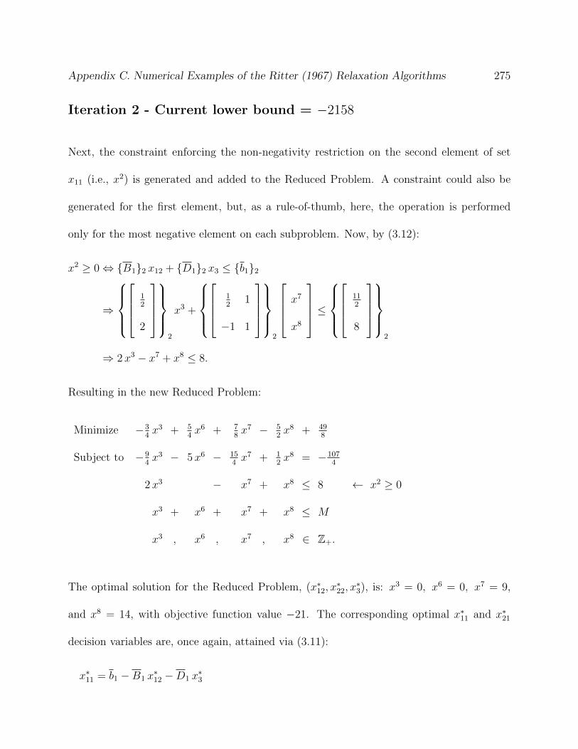
Appendix C. Numerical Examples of the Ritter (1967) Relaxation Algorithms 275
Iteration 2 - Current lower bound = −2158
Next, the constraint enforcing the non-negativity restriction on the second element of set
x11 (i.e., x2) is generated and added to the Reduced Problem. A constraint could also be
generated for the first element, but, as a rule-of-thumb, here, the operation is performed
only for the most negative element on each subproblem. Now, by (3.12):
x2 ≥ 0⇔ {B1}2 x12 + {D1}2 x3 ≤ {b1}2
⇒
12
2
2
x3 +
12
1
−1 1
2
x7
x8
≤
112
8
2
⇒ 2x3 − x7 + x8 ≤ 8.
Resulting in the new Reduced Problem:
Minimize −34x3 + 5
4x6 + 7
8x7 − 5
2x8 + 49
8
Subject to −94x3 − 5x6 − 15
4x7 + 1
2x8 = −107
4
2x3 − x7 + x8 ≤ 8 ← x2 ≥ 0
x3 + x6 + x7 + x8 ≤ M
x3 , x6 , x7 , x8 ∈ Z+.
The optimal solution for the Reduced Problem, (x∗12, x∗22, x
∗3), is: x3 = 0, x6 = 0, x7 = 9,
and x8 = 14, with objective function value −21. The corresponding optimal x∗11 and x∗21
decision variables are, once again, attained via (3.11):
x∗11 = b1 −B1 x∗12 −D1 x
∗3
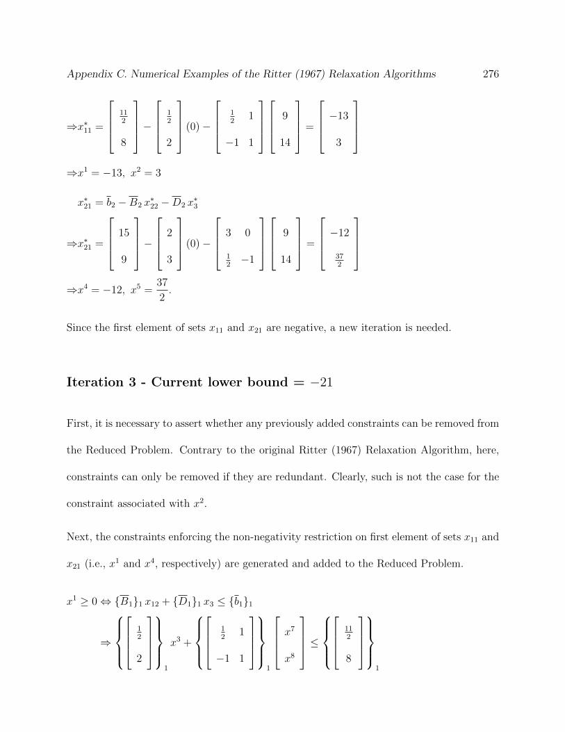
Appendix C. Numerical Examples of the Ritter (1967) Relaxation Algorithms 276
⇒x∗11 =
112
8
−
12
2
(0)−
12
1
−1 1
9
14
=
−13
3
⇒x1 = −13, x2 = 3
x∗21 = b2 −B2 x∗22 −D2 x
∗3
⇒x∗21 =
15
9
−
2
3
(0)−
3 0
12−1
9
14
=
−12
372
⇒x4 = −12, x5 =37
2.
Since the first element of sets x11 and x21 are negative, a new iteration is needed.
Iteration 3 - Current lower bound = −21
First, it is necessary to assert whether any previously added constraints can be removed from
the Reduced Problem. Contrary to the original Ritter (1967) Relaxation Algorithm, here,
constraints can only be removed if they are redundant. Clearly, such is not the case for the
constraint associated with x2.
Next, the constraints enforcing the non-negativity restriction on first element of sets x11 and
x21 (i.e., x1 and x4, respectively) are generated and added to the Reduced Problem.
x1 ≥ 0⇔ {B1}1 x12 + {D1}1 x3 ≤ {b1}1
⇒
12
2
1
x3 +
12
1
−1 1
1
x7
x8
≤
112
8
1

Appendix C. Numerical Examples of the Ritter (1967) Relaxation Algorithms 277
⇒ 1
2x3 +
1
2x7 + x8 ≤ 11
2
x4 ≥ 0⇔ {B2}1 x22 + {D2}1 x3 ≤ {b2}1
⇒
2
3
1
x6 +
3 0
12−1
1
x7
x8
≤
15
9
1
⇒ 2x6 + 3x7 ≤ 15.
Resulting in the new Reduced Problem:
Minimize −34x3 + 5
4x6 + 7
8x7 − 5
2x8 + 49
8
Subject to −94x3 − 5x6 − 15
4x7 + 1
2x8 = −107
4
2x3 − x7 + x8 ≤ 8 ← x2 ≥ 0
12x3 + 1
2x7 + x8 ≤ 11
2← x1 ≥ 0
2x6 + 3x7 ≤ 15 ← x4 ≥ 0
x3 + x6 + x7 + x8 ≤ M
x3 , x6 , x7 , x8 ∈ Z+.
The optimal solution for the Reduced Problem, (x∗12, x∗22, x
∗3), is: x3 = 2, x6 = 4, x7 = 1,
and x8 = 3, with objective function value 3. The corresponding optimal x∗11 and x∗21 decision
variables are, once again, attained via (3.11):
x∗11 = b1 −B1 x∗12 −D1 x
∗3
⇒x∗11 =
112
8
−
12
2
(2)−
12
1
−1 1
1
3
=
1
2
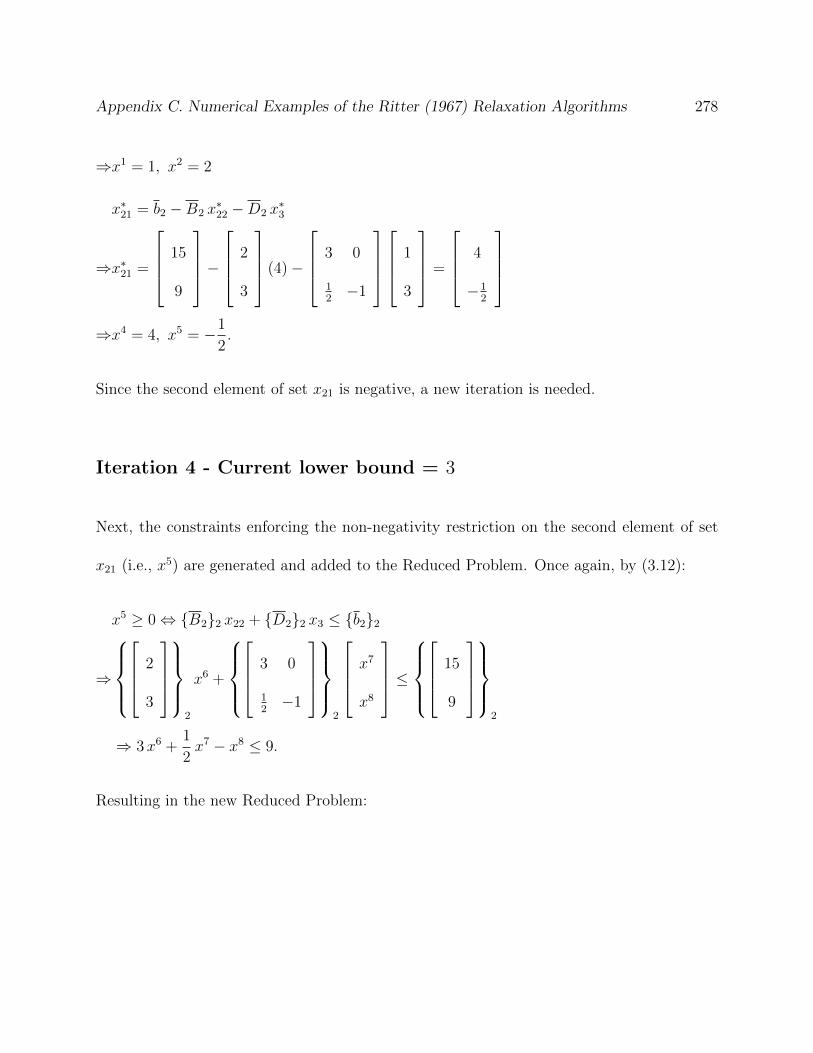
Appendix C. Numerical Examples of the Ritter (1967) Relaxation Algorithms 278
⇒x1 = 1, x2 = 2
x∗21 = b2 −B2 x∗22 −D2 x
∗3
⇒x∗21 =
15
9
−
2
3
(4)−
3 0
12−1
1
3
=
4
−12
⇒x4 = 4, x5 = −1
2.
Since the second element of set x21 is negative, a new iteration is needed.
Iteration 4 - Current lower bound = 3
Next, the constraints enforcing the non-negativity restriction on the second element of set
x21 (i.e., x5) are generated and added to the Reduced Problem. Once again, by (3.12):
x5 ≥ 0⇔ {B2}2 x22 + {D2}2 x3 ≤ {b2}2
⇒
2
3
2
x6 +
3 0
12−1
2
x7
x8
≤
15
9
2
⇒ 3x6 +1
2x7 − x8 ≤ 9.
Resulting in the new Reduced Problem:
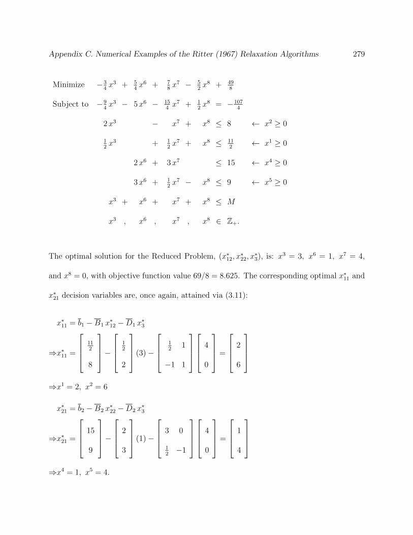
Appendix C. Numerical Examples of the Ritter (1967) Relaxation Algorithms 279
Minimize −34x3 + 5
4x6 + 7
8x7 − 5
2x8 + 49
8
Subject to −94x3 − 5x6 − 15
4x7 + 1
2x8 = −107
4
2x3 − x7 + x8 ≤ 8 ← x2 ≥ 0
12x3 + 1
2x7 + x8 ≤ 11
2← x1 ≥ 0
2x6 + 3x7 ≤ 15 ← x4 ≥ 0
3x6 + 12x7 − x8 ≤ 9 ← x5 ≥ 0
x3 + x6 + x7 + x8 ≤ M
x3 , x6 , x7 , x8 ∈ Z+.
The optimal solution for the Reduced Problem, (x∗12, x∗22, x
∗3), is: x3 = 3, x6 = 1, x7 = 4,
and x8 = 0, with objective function value 69/8 = 8.625. The corresponding optimal x∗11 and
x∗21 decision variables are, once again, attained via (3.11):
x∗11 = b1 −B1 x∗12 −D1 x
∗3
⇒x∗11 =
112
8
−
12
2
(3)−
12
1
−1 1
4
0
=
2
6
⇒x1 = 2, x2 = 6
x∗21 = b2 −B2 x∗22 −D2 x
∗3
⇒x∗21 =
15
9
−
2
3
(1)−
3 0
12−1
4
0
=
1
4
⇒x4 = 1, x5 = 4.

Appendix C. Numerical Examples of the Ritter (1967) Relaxation Algorithms 280
Since all elements of sets x11 and x21 are non-negative and integer, the algorithm terminates
with optimal solution: x1 = 2, x2 = 6, x3 = 3, x4 = 1, x5 = 4, x6 = 1, x7 = 4, and x8 = 0,
and objective function value of 69/8 = 8.625.
Observe that the integer restriction on the relaxed variables was direct consequence of an
integer solution to the Reduced Problem, that is, given that x3 = 3, x6 = 1, x7 = 4, and
x8 = 0, the original problem simplifies to:
Minimize x1 + 12x2 + 3
4(3) + 3
8x4 − x5 − (1) + 3
2(4)
Subject to 2x1 + (3) + (4) + 2 (0) = 11
x2 + 2(3) − (4) + (0) = 8
+ 13x4 + 2
3(1) + (4) = 5
x5 + 3(1) + 12(4) − (0) = 9
12x1 + x2 + x4 + x5 − (4) + (0) = 8
x1 , x2 , x4 , x5 ∈ Z+,
Or, more specifically, to:

Appendix C. Numerical Examples of the Ritter (1967) Relaxation Algorithms 281
Minimize x1 + 12x2 + 3
8x4 − x5 + 29
4
Subject to 2x1 = 4
x2 = 6
13x4 = 1
3
x5 = 4
12x1 + x2 + x4 + x5 = 12
x1 , x2 , x4 , x5 ∈ Z+.
Clearly, the last structural constraint (i.e., the complicating constraint) is redundant, and
the system of equations has the unique solution x1 = 2, x2 = 6, x4 = 1, and x5 = 4, with
objective function value of 69/8 = 8.625. Next, a more interesting version of the problem,
namely its application to mixed-integer problems is exemplified.
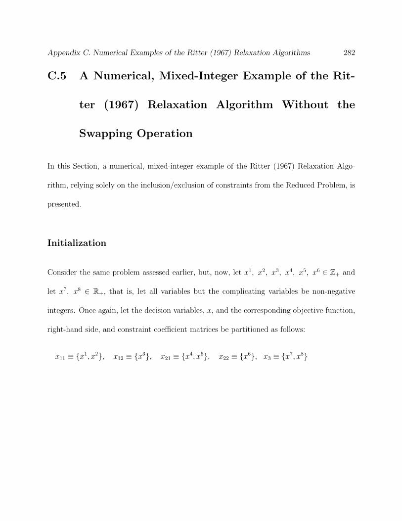
Appendix C. Numerical Examples of the Ritter (1967) Relaxation Algorithms 282
C.5 A Numerical, Mixed-Integer Example of the Rit-
ter (1967) Relaxation Algorithm Without the
Swapping Operation
In this Section, a numerical, mixed-integer example of the Ritter (1967) Relaxation Algo-
rithm, relying solely on the inclusion/exclusion of constraints from the Reduced Problem, is
presented.
Initialization
Consider the same problem assessed earlier, but, now, let x1, x2, x3, x4, x5, x6 ∈ Z+ and
let x7, x8 ∈ R+, that is, let all variables but the complicating variables be non-negative
integers. Once again, let the decision variables, x, and the corresponding objective function,
right-hand side, and constraint coefficient matrices be partitioned as follows:
x11 ≡ {x1, x2}, x12 ≡ {x3}, x21 ≡ {x4, x5}, x22 ≡ {x6}, x3 ≡ {x7, x8}
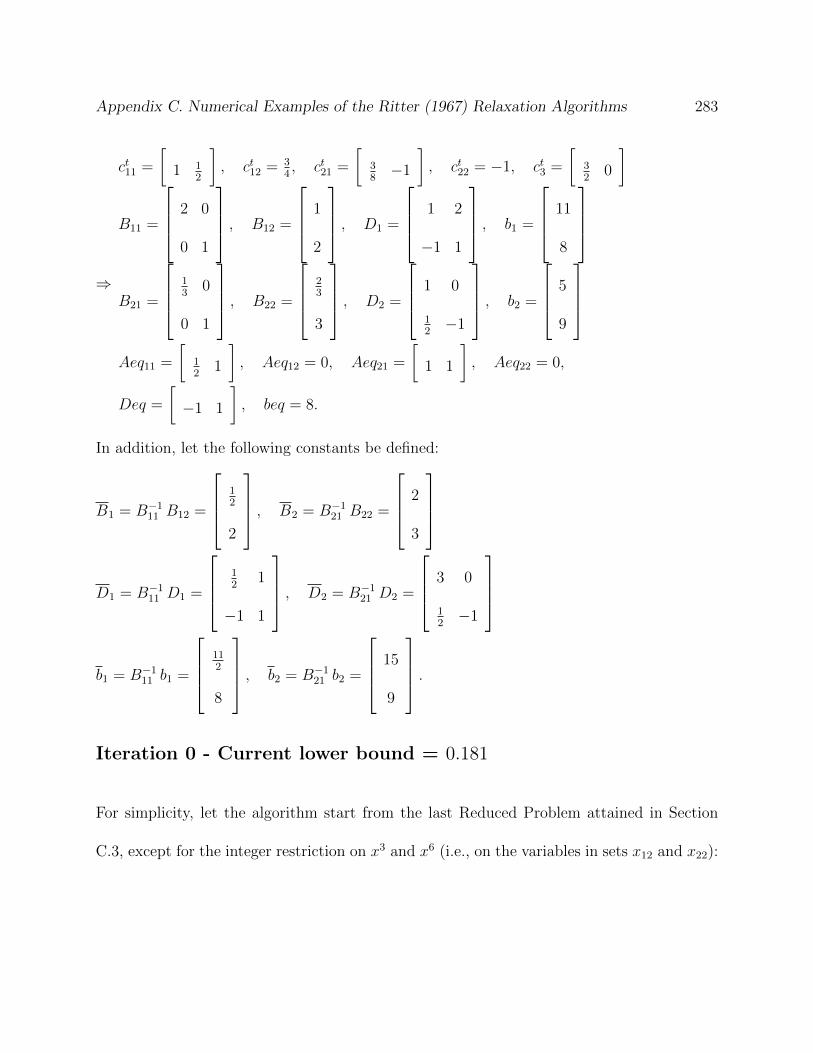
Appendix C. Numerical Examples of the Ritter (1967) Relaxation Algorithms 283
⇒
ct11 =
[1 1
2
], ct12 = 3
4, ct21 =
[38−1
], ct22 = −1, ct3 =
[32
0
]
B11 =
2 0
0 1
, B12 =
1
2
, D1 =
1 2
−1 1
, b1 =
11
8
B21 =
13
0
0 1
, B22 =
23
3
, D2 =
1 0
12−1
, b2 =
5
9
Aeq11 =
[12
1
], Aeq12 = 0, Aeq21 =
[1 1
], Aeq22 = 0,
Deq =
[−1 1
], beq = 8.
In addition, let the following constants be defined:
B1 = B−111 B12 =
12
2
, B2 = B−1
21 B22 =
2
3
D1 = B−111 D1 =
12
1
−1 1
, D2 = B−1
21 D2 =
3 0
12−1
b1 = B−111 b1 =
112
8
, b2 = B−1
21 b2 =
15
9
.
Iteration 0 - Current lower bound = 0.181
For simplicity, let the algorithm start from the last Reduced Problem attained in Section
C.3, except for the integer restriction on x3 and x6 (i.e., on the variables in sets x12 and x22):
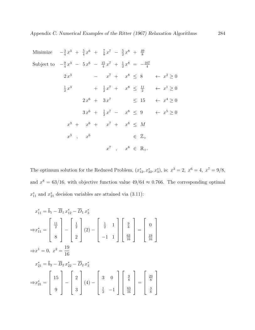
Appendix C. Numerical Examples of the Ritter (1967) Relaxation Algorithms 284
Minimize −34x3 + 5
4x6 + 7
8x7 − 5
2x8 + 49
8
Subject to −94x3 − 5x6 − 15
4x7 + 1
2x8 = −107
4
2x3 − x7 + x8 ≤ 8 ← x2 ≥ 0
12x3 + 1
2x7 + x8 ≤ 11
2← x1 ≥ 0
2x6 + 3x7 ≤ 15 ← x4 ≥ 0
3x6 + 12x7 − x8 ≤ 9 ← x5 ≥ 0
x3 + x6 + x7 + x8 ≤ M
x3 , x6 ∈ Z+
x7 , x8 ∈ R+.
The optimum solution for the Reduced Problem, (x∗12, x∗22, x
∗3), is: x3 = 2, x6 = 4, x7 = 9/8,
and x8 = 63/16, with objective function value 49/64 ≈ 0.766. The corresponding optimal
x∗11 and x∗21 decision variables are attained via (3.11):
x∗11 = b1 −B1 x∗12 −D1 x
∗3
⇒x∗11 =
112
8
−
12
2
(2)−
12
1
−1 1
98
6316
=
0
1916
⇒x1 = 0, x2 =19
16
x∗21 = b2 −B2 x∗22 −D2 x
∗3
⇒x∗21 =
15
9
−
2
3
(4)−
3 0
12−1
98
6316
=
298
38
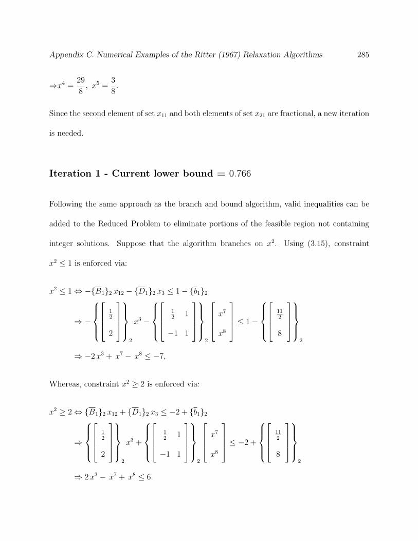
Appendix C. Numerical Examples of the Ritter (1967) Relaxation Algorithms 285
⇒x4 =29
8, x5 =
3
8.
Since the second element of set x11 and both elements of set x21 are fractional, a new iteration
is needed.
Iteration 1 - Current lower bound = 0.766
Following the same approach as the branch and bound algorithm, valid inequalities can be
added to the Reduced Problem to eliminate portions of the feasible region not containing
integer solutions. Suppose that the algorithm branches on x2. Using (3.15), constraint
x2 ≤ 1 is enforced via:
x2 ≤ 1⇔ −{B1}2 x12 − {D1}2 x3 ≤ 1− {b1}2
⇒ −
12
2
2
x3 −
12
1
−1 1
2
x7
x8
≤ 1−
112
8
2
⇒ −2x3 + x7 − x8 ≤ −7,
Whereas, constraint x2 ≥ 2 is enforced via:
x2 ≥ 2⇔ {B1}2 x12 + {D1}2 x3 ≤ −2 + {b1}2
⇒
12
2
2
x3 +
12
1
−1 1
2
x7
x8
≤ −2 +
112
8
2
⇒ 2x3 − x7 + x8 ≤ 6.
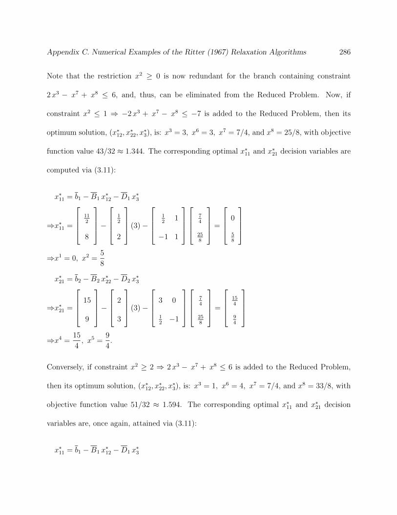
Appendix C. Numerical Examples of the Ritter (1967) Relaxation Algorithms 286
Note that the restriction x2 ≥ 0 is now redundant for the branch containing constraint
2x3 − x7 + x8 ≤ 6, and, thus, can be eliminated from the Reduced Problem. Now, if
constraint x2 ≤ 1 ⇒ −2x3 + x7 − x8 ≤ −7 is added to the Reduced Problem, then its
optimum solution, (x∗12, x∗22, x
∗3), is: x3 = 3, x6 = 3, x7 = 7/4, and x8 = 25/8, with objective
function value 43/32 ≈ 1.344. The corresponding optimal x∗11 and x∗21 decision variables are
computed via (3.11):
x∗11 = b1 −B1 x∗12 −D1 x
∗3
⇒x∗11 =
112
8
−
12
2
(3)−
12
1
−1 1
74
258
=
0
58
⇒x1 = 0, x2 =5
8
x∗21 = b2 −B2 x∗22 −D2 x
∗3
⇒x∗21 =
15
9
−
2
3
(3)−
3 0
12−1
74
258
=
154
94
⇒x4 =15
4, x5 =
9
4.
Conversely, if constraint x2 ≥ 2 ⇒ 2x3 − x7 + x8 ≤ 6 is added to the Reduced Problem,
then its optimum solution, (x∗12, x∗22, x
∗3), is: x3 = 1, x6 = 4, x7 = 7/4, and x8 = 33/8, with
objective function value 51/32 ≈ 1.594. The corresponding optimal x∗11 and x∗21 decision
variables are, once again, attained via (3.11):
x∗11 = b1 −B1 x∗12 −D1 x
∗3

Appendix C. Numerical Examples of the Ritter (1967) Relaxation Algorithms 287
⇒x∗11 =
112
8
−
12
2
(1)−
12
1
−1 1
74
338
=
0
298
⇒x1 = 0, x2 =29
8
x∗21 = b2 −B2 x∗22 −D2 x
∗3
⇒x∗21 =
15
9
−
2
3
(4)−
3 0
12−1
74
338
=
74
14
⇒x4 =7
4, x5 =
1
4.
The initial branch and bound tree is presented in Figure C.1.
1
0
2
Figure C.1: First iteration of the branch and bound algorithm.
Since neither branch of the tree results in an integer solution, neither can be fathomed, and
a new iteration is needed.
Iteration 2 - Current lower bound = 1.344
In order to maintain this example somewhat brief, instead of branching on every possible
decision variable, a depth-first approach will be used for the branch leading to the optimum
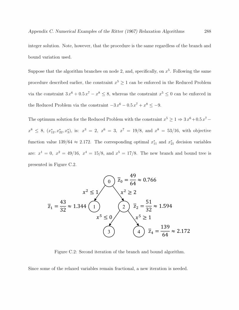
Appendix C. Numerical Examples of the Ritter (1967) Relaxation Algorithms 288
integer solution. Note, however, that the procedure is the same regardless of the branch and
bound variation used.
Suppose that the algorithm branches on node 2, and, specifically, on x5. Following the same
procedure described earlier, the constraint x5 ≥ 1 can be enforced in the Reduced Problem
via the constraint 3 x6 + 0.5x7 − x8 ≤ 8, whereas the constraint x5 ≤ 0 can be enforced in
the Reduced Problem via the constraint −3x6 − 0.5x7 + x8 ≤ −9.
The optimum solution for the Reduced Problem with the constraint x5 ≥ 1⇒ 3x6 +0.5x7−
x8 ≤ 8, (x∗12, x∗22, x
∗3), is: x3 = 2, x6 = 3, x7 = 19/8, and x8 = 53/16, with objective
function value 139/64 ≈ 2.172. The corresponding optimal x∗11 and x∗21 decision variables
are: x1 = 0, x2 = 49/16, x4 = 15/8, and x5 = 17/8. The new branch and bound tree is
presented in Figure C.2.
1
0
2
3 4
Figure C.2: Second iteration of the branch and bound algorithm.
Since some of the relaxed variables remain fractional, a new iteration is needed.
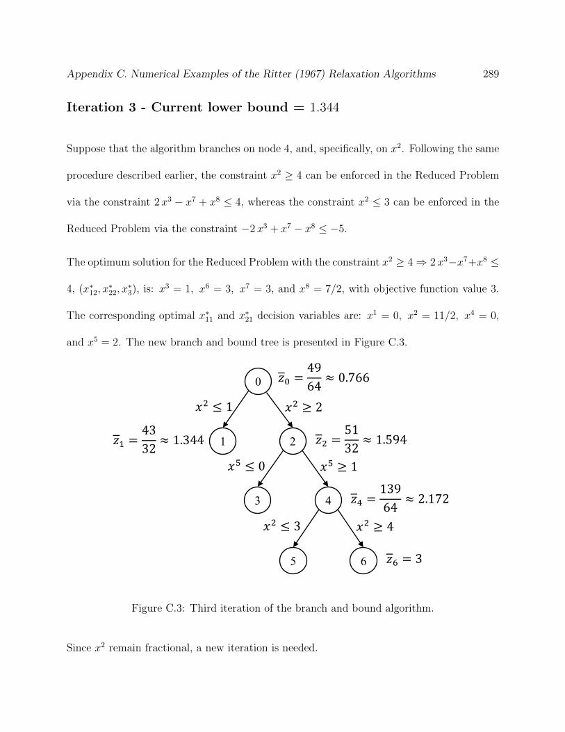
Appendix C. Numerical Examples of the Ritter (1967) Relaxation Algorithms 289
Iteration 3 - Current lower bound = 1.344
Suppose that the algorithm branches on node 4, and, specifically, on x2. Following the same
procedure described earlier, the constraint x2 ≥ 4 can be enforced in the Reduced Problem
via the constraint 2x3 − x7 + x8 ≤ 4, whereas the constraint x2 ≤ 3 can be enforced in the
Reduced Problem via the constraint −2x3 + x7 − x8 ≤ −5.
The optimum solution for the Reduced Problem with the constraint x2 ≥ 4⇒ 2x3−x7+x8 ≤
4, (x∗12, x∗22, x
∗3), is: x3 = 1, x6 = 3, x7 = 3, and x8 = 7/2, with objective function value 3.
The corresponding optimal x∗11 and x∗21 decision variables are: x1 = 0, x2 = 11/2, x4 = 0,
and x5 = 2. The new branch and bound tree is presented in Figure C.3.
1
0
2
3 4
5 6
Figure C.3: Third iteration of the branch and bound algorithm.
Since x2 remain fractional, a new iteration is needed.
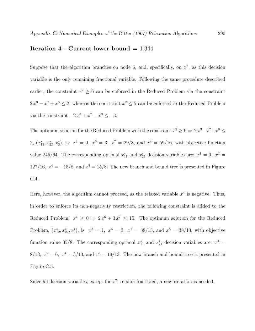
Appendix C. Numerical Examples of the Ritter (1967) Relaxation Algorithms 290
Iteration 4 - Current lower bound = 1.344
Suppose that the algorithm branches on node 6, and, specifically, on x2, as this decision
variable is the only remaining fractional variable. Following the same procedure described
earlier, the constraint x2 ≥ 6 can be enforced in the Reduced Problem via the constraint
2x3 − x7 + x8 ≤ 2, whereas the constraint x2 ≤ 5 can be enforced in the Reduced Problem
via the constraint −2x3 + x7 − x8 ≤ −3.
The optimum solution for the Reduced Problem with the constraint x2 ≥ 6⇒ 2x3−x7+x8 ≤
2, (x∗12, x∗22, x
∗3), is: x3 = 0, x6 = 3, x7 = 29/8, and x8 = 59/16, with objective function
value 245/64. The corresponding optimal x∗11 and x∗21 decision variables are: x1 = 0, x2 =
127/16, x4 = −15/8, and x5 = 15/8. The new branch and bound tree is presented in Figure
C.4.
Here, however, the algorithm cannot proceed, as the relaxed variable x4 is negative. Thus,
in order to enforce its non-negativity restriction, the following constraint is added to the
Reduced Problem: x4 ≥ 0 ⇒ 2x6 + 3 x7 ≤ 15. The optimum solution for the Reduced
Problem, (x∗12, x∗22, x
∗3), is: x3 = 1, x6 = 3, x7 = 38/13, and x8 = 38/13, with objective
function value 35/8. The corresponding optimal x∗11 and x∗21 decision variables are: x1 =
8/13, x2 = 6, x4 = 3/13, and x5 = 19/13. The new branch and bound tree is presented in
Figure C.5.
Since all decision variables, except for x2, remain fractional, a new iteration is needed.
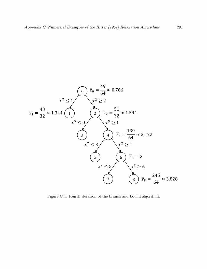
Appendix C. Numerical Examples of the Ritter (1967) Relaxation Algorithms 291
1
0
2
3 4
5 6
7 8
Figure C.4: Fourth iteration of the branch and bound algorithm.
Appendix C. Numerical Examples of the Ritter (1967) Relaxation Algorithms 292
1
0
2
3 4
5 6
7 8
9
Figure C.5: Fourth iteration of the branch and bound algorithm, after a new non-negativity
restriction is enforced.

Appendix C. Numerical Examples of the Ritter (1967) Relaxation Algorithms 293
Iteration 5 - Current lower bound = 1.344
Suppose that the algorithm branches on node 9, and, specifically, on x4, as this decision
variable is closest to an integer solution. Following the same procedure described earlier, the
constraint x4 ≥ 1 can be enforced in the Reduced Problem via the constraint 2x6+3 x7 ≤ 14,
whereas the constraint x4 ≤ 0 can be enforced in the Reduced Problem via the constraint
−2x6 − 3x7 ≤ 15. The Reduced Problem (after the redundant constraints are removed)
including the constraint x4 ≥ 1⇒ 2x6 + 3x7 ≤ 14 is as follows:
Minimize −34x3 + 5
4x6 + 7
8x7 − 5
2x8 + 49
8
Subject to −94x3 − 5x6 − 15
4x7 + 1
2x8 = −107
4
2x3 − x7 + x8 ≤ 2 ← x2 ≥ 6
12x3 + 1
2x7 + x8 ≤ 11
2← x1 ≥ 0
2x6 + 3x7 ≤ 14 ← x4 ≥ 1
3x6 + 12x7 − x8 ≤ 8 ← x5 ≥ 1
x3 + x6 + x7 + x8 ≤ M
x3 , x6 ∈ Z+
x7 , x8 ∈ R+.
The optimum solution for this Reduced Problem, (x∗12, x∗22, x
∗3), is: x3 = 3, x6 = 1, x7 = 4,
and x8 = 0, with objective function value 69/8 = 8.625. The corresponding optimal x∗11 and
x∗21 decision variables are: x1 = 2, x2 = 6, x4 = 1, and x5 = 4. Since all integer-restricted
decision variables are integer, the branch is fathomed. The final branch and bound tree is
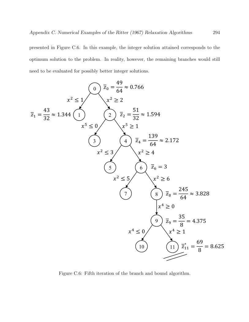
Appendix C. Numerical Examples of the Ritter (1967) Relaxation Algorithms 294
presented in Figure C.6. In this example, the integer solution attained corresponds to the
optimum solution to the problem. In reality, however, the remaining branches would still
need to be evaluated for possibly better integer solutions.
1
0
2
3 4
5 6
7 8
9
10 11
Figure C.6: Fifth iteration of the branch and bound algorithm.

Appendix C. Numerical Examples of the Ritter (1967) Relaxation Algorithms 295
C.6 A Numerical, Mixed-Integer, Quadratic Example
of the Ritter (1967) Relaxation Algorithm With-
out the Swapping Operation
In this Section, a numerical, mixed-integer example of the Ritter (1967) Relaxation Algo-
rithm, relying solely on the inclusion/exclusion of constraints from the Reduced Problem,
is presented. Consider the following, bordered (or arrowhead) structure, mixed-integer pro-
gramming problem. As before, let x1, x2, x3, x4, x5, x6 ∈ Z+ and let x7, x8 ∈ R+, that
is, let all variables but the complicating variables be non-negative integers. Observe that
such example problem differs from the ones assessed in previous sections, as it includes a
quadratic objective function and both complicating equality and inequality constraints.

Appendix C. Numerical Examples of the Ritter (1967) Relaxation Algorithms 296
Minimize (x1 + 12x2 + 3
4x3 + 3
8x4 − x5 − x6 + 3
2x7)2 +
x1 + 12x2 + 3
4x3 + 3
8x4 − x5 − x6 + 3
2x7
Subject to 2x1 + x3 + x7 + 2x8 = 11
x2 + 2 x3 − x7 + x8 = 8
+ 13x4 + 2
3x6 + x7 = 5
x5 + 3 x6 + 12x7 − x8 = 9
x2 + x3 + x5 − x7 − x8 = 0
x1 + x2 + x4 + x7 + x8 = 14
12x1 + x2 + 1
2x4 + x5 − x7 + x8 ≤ 15
−x1 + x2 − x3 + x4 − x5 + x6 − x7 + x8 ≤ 15
x1 , x2 , x3 , x4 , x5 , x6 ∈ Z+
x7 , x8 ∈ R+
Initialization
Since the subproblem constraint coefficients are identical to those in previous examples, it
follows that the decision variables could be similarly partitioned. However, for completeness,
suppose that a different partitioning scheme is selected upon initialization, namely:
x11 ≡ {x1, x3}, x12 ≡ {x2}, x21 ≡ {x5, x6}, x22 ≡ {x4}, x3 ≡ {x7, x8}

Appendix C. Numerical Examples of the Ritter (1967) Relaxation Algorithms 297
⇒
ct11 =
[1 3
4
], ct12 = 1
2, ct21 =
[−1 −1
], ct22 = 3
8, ct3 =
[32
0
]
B11 =
2 1
0 2
, B12 =
0
1
, D1 =
1 2
−1 1
, b1 =
11
8
B21 =
0 23
1 3
, B22 =
13
0
, D2 =
1 0
12−1
, b2 =
5
9
Aeq11 =
0 1
1 0
, Aeq12 =
1
1
, Aeq21 =
1 0
0 0
, Aeq22 =
0
1
,
Deq =
−1 −1
1 1
, beq =
0
14
Aineq11 =
12
0
−1 −1
, Aineq12 =
1
1
, Aineq21 =
1 0
−1 1
,
Aineq22 =
12
1
, Dineq =
−1 1
−1 1
, bineq =
15
15
.
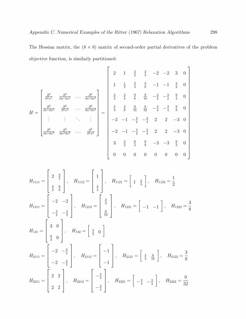
Appendix C. Numerical Examples of the Ritter (1967) Relaxation Algorithms 298
The Hessian matrix, the (8 × 8) matrix of second-order partial derivatives of the problem
objective function, is similarly partitioned:
H =
∂2
∂2x1∂2
∂x1∂x2. . . ∂2
∂x1∂x8
∂2
∂x1∂x2∂2
∂2x2. . . ∂2
∂x2∂x8
......
. . ....
∂2
∂x1∂x8∂2
∂x2∂x8. . . ∂2
∂2x8
=
2 1 32
34−2 −2 3 0
1 12
34
38−1 −1 3
20
32
34
98
916−3
2−3
294
0
34
38
916
932−3
4−3
498
0
−2 −1 −32−3
42 2 −3 0
−2 −1 −32−3
42 2 −3 0
3 32
94
98−3 −3 9
20
0 0 0 0 0 0 0 0
H1111 =
2 32
32
98
, H1112 =
1
34
, H1121 =
[1 3
4
], H1122 =
1
2
H1211 =
−2 −2
−32−3
2
, H1212 =
34
916
, H1221 =
[−1 −1
], H1222 =
3
8
H131 =
3 0
94
0
, H132 =
[32
0
]
H2111 =
−2 −3
2
−2 −32
, H2112 =
−1
−1
, H2121 =
[34
916
], H2122 =
3
8
H2211 =
2 2
2 2
, H2212 =
−3
4
−34
, H2221 =
[−3
4−3
4
], H2222 =
9
32
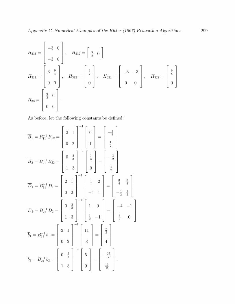
Appendix C. Numerical Examples of the Ritter (1967) Relaxation Algorithms 299
H231 =
−3 0
−3 0
, H232 =
[98
0
]
H311 =
3 94
0 0
, H312 =
32
0
, H321 =
−3 −3
0 0
, H322 =
98
0
H33 =
92
0
0 0
.
As before, let the following constants be defined:
B1 = B−111 B12 =
2 1
0 2
−1
0
1
=
−1
4
12
B2 = B−121 B22 =
0 23
1 3
−1
13
0
=
−3
2
12
D1 = B−111 D1 =
2 1
0 2
−1
1 2
−1 1
=
34
34
−12
12
D2 = B−121 D2 =
0 23
1 3
−1
1 0
12−1
=
−4 −1
32
0
b1 = B−111 b1 =
2 1
0 2
−1
11
8
=
72
4
b2 = B−121 b2 =
0 23
1 3
−1
5
9
=
−27
2
152
.

Appendix C. Numerical Examples of the Ritter (1967) Relaxation Algorithms 300
Next, the Reduced Problem parameters are computed via equations (3.13) and, since the
objective function is quadratic, (3.18). Matrix operations are omitted for brevity.
Ljk = Hjk22 −Bt
jHjk12 −Hjk21Bk +Bt
jHjk11Bk, ∀ j = 1, · · · , p, k = 1, · · · , p
⇒L11 =9
32, L12 = −15
32, L21 = −15
32, L22 =
25
32
Lj(p+1) = Hj(p+1)2 −Bt
jHj(p+1)1 +
p∑
k=1
(Bt
jHjk11 −Hjk21
)Dk, ∀ j = 1, · · · , p
⇒L13 =
[−33
32−51
32
], L23 =
[5532
8532
]
L(p+1)k = H(p+1)k2 −H(p+1)k1Bk +
p∑
j=1
Dt
j
(Hjk11Bk −Hjk12
), ∀ k = 1, · · · , p
⇒L31 =
−33
32
−5132
, L32 =
5532
8532
L(p+1)(p+1) = H(p+1)(p+1) −p∑
j=1
(Dt
jHj(p+1)1 +H(p+1)j1Dj
)+
p∑
j=1
p∑
k=1
Dt
jHjk11Dk
⇒L33 =
12132
18732
18732
28932
dtj = ctj2 − ctj1Bj +1
2
p∑
k=1
bt
k
(H tjk21 −H t
jk11Bj +Hkj12 −Hkj11Bj
), ∀ j = 1, · · · , p
⇒dt1 =39
4, dt2 = −65
4
dtp+1 = ctp+1 −p∑
j=1
(ctj1Dj −
1
2bt
j
(Hj(p+1)1 +H t
(p+1)j1
)+
1
2
p∑
k=1
bt
j
(Hjk11 +H t
kj11
)Dk
)
⇒dt3 =
[−143
4−221
4
]
α =
p∑
j=1
(ctj1bj +
1
2
p∑
k=1
bt
jHjk11bk
)
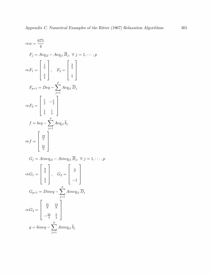
Appendix C. Numerical Examples of the Ritter (1967) Relaxation Algorithms 301
⇒α =675
4
Fj = Aeqj2 − Aeqj1Bj, ∀ j = 1, · · · , p
⇒F1 =
12
54
, F2 =
32
1
Fp+1 = Deq −p∑
j=1
Aeqj1Dj
⇒F3 =
72−1
2
14
14
f = beq −p∑
j=1
Aeqj1 bj
⇒f =
192
212
Gj = Aineqj2 − Aineqj1Bj, ∀ j = 1, · · · , p
⇒G1 =
98
54
, G2 =
2
−1
Gp+1 = Dineq −p∑
j=1
Aineqj1Dj
⇒G3 =
218
138
−254
54
g = bineq −p∑
j=1
Aineqj1 bj

Appendix C. Numerical Examples of the Ritter (1967) Relaxation Algorithms 302
⇒g =
1074
32
.
After merging the Ljk, j = 1, · · · , 3, k = 1, · · · , 3 matrices into a larger, Hessian matrix, it
follows that the objective function of the Reduced Problem is given by:
Minimize1
2
[x2 x4 x7 x8
]
932
−1532−33
32−51
32
−1532
2532
5532
8532
−3332
5532
12132
18732
−5132
8532
18732
28932
x2
x4
x7
x8
+
[394−65
4−143
4−221
4
]
x2
x4
x7
x8
+675
4,
Or, after some simplification:
Minimize
(−3
8x2 +
5
8x4 +
11
8x7 +
17
8x8
)2
+39
4x2 − 65
4x4 − 143
4x7 − 221
4x8 +
675
4.
Consequently, the initial Reduced Problem is as follows:
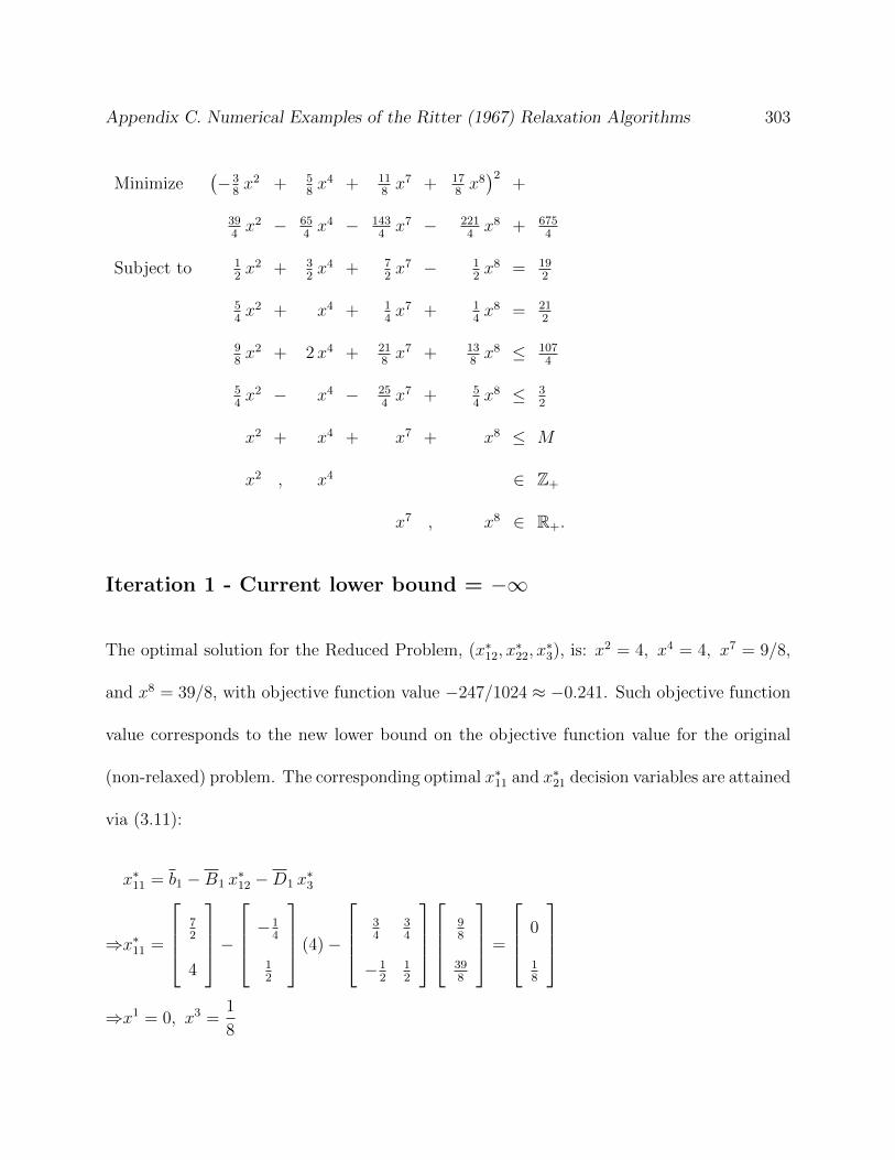
Appendix C. Numerical Examples of the Ritter (1967) Relaxation Algorithms 303
Minimize(−3
8x2 + 5
8x4 + 11
8x7 + 17
8x8)2
+
394x2 − 65
4x4 − 143
4x7 − 221
4x8 + 675
4
Subject to 12x2 + 3
2x4 + 7
2x7 − 1
2x8 = 19
2
54x2 + x4 + 1
4x7 + 1
4x8 = 21
2
98x2 + 2x4 + 21
8x7 + 13
8x8 ≤ 107
4
54x2 − x4 − 25
4x7 + 5
4x8 ≤ 3
2
x2 + x4 + x7 + x8 ≤ M
x2 , x4 ∈ Z+
x7 , x8 ∈ R+.
Iteration 1 - Current lower bound = −∞
The optimal solution for the Reduced Problem, (x∗12, x∗22, x
∗3), is: x2 = 4, x4 = 4, x7 = 9/8,
and x8 = 39/8, with objective function value −247/1024 ≈ −0.241. Such objective function
value corresponds to the new lower bound on the objective function value for the original
(non-relaxed) problem. The corresponding optimal x∗11 and x∗21 decision variables are attained
via (3.11):
x∗11 = b1 −B1 x∗12 −D1 x
∗3
⇒x∗11 =
72
4
−
−1
4
12
(4)−
34
34
−12
12
98
398
=
0
18
⇒x1 = 0, x3 =1
8

Appendix C. Numerical Examples of the Ritter (1967) Relaxation Algorithms 304
x∗21 = b2 −B2 x∗22 −D2 x
∗3
⇒x∗21 =
−27
2
152
−
−3
2
12
(4)−
−4 −1
32
0
98
398
=
158
6116
⇒x5 =15
8, x6 =
61
16.
Since the second element of set x11 and both elements of set x21 are fractional, a new iteration
is needed.
Iteration 2 - Current lower bound = −0.241
Following the same approach as the branch and bound algorithm, valid inequalities can be
added to the Reduced Problem to eliminate portions of the feasible region not containing
integer solutions. Suppose that the algorithm branches on x3. Using (3.15), constraint
x3 ≤ 0 is enforced via:
x3 ≤ 0⇔ −{B1}2 x12 − {D1}2 x3 ≤ 0− {b1}2
⇒ −
−1
4
12
2
x2 −
34
34
−12
12
2
x7
x8
≤ 0−
72
4
2
⇒ −1
2x2 +
1
2x7 − 1
2x8 ≤ −4,
Whereas, constraint x3 ≥ 1 is enforced via:
x3 ≥ 1⇔ {B1}2 x12 + {D1}2 x3 ≤ −1 + {b1}2
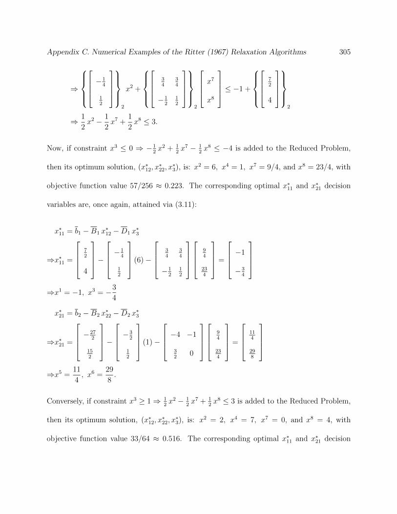
Appendix C. Numerical Examples of the Ritter (1967) Relaxation Algorithms 305
⇒
−1
4
12
2
x2 +
34
34
−12
12
2
x7
x8
≤ −1 +
72
4
2
⇒ 1
2x2 − 1
2x7 +
1
2x8 ≤ 3.
Now, if constraint x3 ≤ 0 ⇒ −12x2 + 1
2x7 − 1
2x8 ≤ −4 is added to the Reduced Problem,
then its optimum solution, (x∗12, x∗22, x
∗3), is: x2 = 6, x4 = 1, x7 = 9/4, and x8 = 23/4, with
objective function value 57/256 ≈ 0.223. The corresponding optimal x∗11 and x∗21 decision
variables are, once again, attained via (3.11):
x∗11 = b1 −B1 x∗12 −D1 x
∗3
⇒x∗11 =
72
4
−
−1
4
12
(6)−
34
34
−12
12
94
234
=
−1
−34
⇒x1 = −1, x3 = −3
4
x∗21 = b2 −B2 x∗22 −D2 x
∗3
⇒x∗21 =
−27
2
152
−
−3
2
12
(1)−
−4 −1
32
0
94
234
=
114
298
⇒x5 =11
4, x6 =
29
8.
Conversely, if constraint x3 ≥ 1⇒ 12x2 − 1
2x7 + 1
2x8 ≤ 3 is added to the Reduced Problem,
then its optimum solution, (x∗12, x∗22, x
∗3), is: x2 = 2, x4 = 7, x7 = 0, and x8 = 4, with
objective function value 33/64 ≈ 0.516. The corresponding optimal x∗11 and x∗21 decision
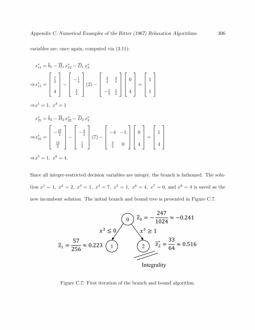
Appendix C. Numerical Examples of the Ritter (1967) Relaxation Algorithms 306
variables are, once again, computed via (3.11):
x∗11 = b1 −B1 x∗12 −D1 x
∗3
⇒x∗11 =
72
4
−
−1
4
12
(2)−
34
34
−12
12
0
4
=
1
1
⇒x1 = 1, x3 = 1
x∗21 = b2 −B2 x∗22 −D2 x
∗3
⇒x∗21 =
−27
2
152
−
−3
2
12
(7)−
−4 −1
32
0
0
4
=
1
4
⇒x5 = 1, x6 = 4.
Since all integer-restricted decision variables are integer, the branch is fathomed. The solu-
tion x1 = 1, x2 = 2, x3 = 1, x4 = 7, x5 = 1, x6 = 4, x7 = 0, and x8 = 4 is saved as the
new incumbent solution. The initial branch and bound tree is presented in Figure C.7.
1
0
2
Integrality
Figure C.7: First iteration of the branch and bound algorithm.

Appendix C. Numerical Examples of the Ritter (1967) Relaxation Algorithms 307
Iteration 3 - Current lower bound = 0.223, Incumbent Obj. = 0.516
As before, the algorithm would branch on node 1, as such is the only node still active.
However, since both elements of set x11 are negative, first a constraint enforcing the non-
negativity restriction of x1 is generated and added to the Reduced Problem. Observe that a
similar constraint could be generated for x3, but, as a rule-of-thumb, here, the operation is
performed only for the most negative element on each subproblem. Now, by (3.12):
x1 ≥ 0⇔ {B1}1 x12 + {D1}1 x3 ≤ {b1}1
⇒
−1
4
12
1
x2 +
34
34
−12
12
1
x7
x8
≤
72
4
1
⇒ −1
4x2 +
3
4x7 +
3
4x8 ≤ 7
2.
The optimum solution for the Reduced Problem, (x∗12, x∗22, x
∗3), is: x2 = 7, x4 = 0, x7 = 19/8,
and x8 = 37/8, with objective function value 979/159 ≈ 6.157. The corresponding optimal
x∗11 and x∗21 decision variables are, once again, computed via (3.11):
x∗11 = b1 −B1 x∗12 −D1 x
∗3
⇒x∗11 =
72
4
−
−1
4
12
(7)−
34
34
−12
12
198
378
=
0
−58
⇒x1 = 0, x3 = −5
8
x∗21 = b2 −B2 x∗22 −D2 x
∗3

Appendix C. Numerical Examples of the Ritter (1967) Relaxation Algorithms 308
⇒x∗21 =
−27
2
152
−
−3
2
12
(0)−
−4 −1
32
0
198
378
=
58
6316
⇒x5 =5
8, x6 =
63
16.
Since the second element of set x11 is negative, it would appear that another iteration is
needed. However, note that the current objective function value for the node is higher than
the objective function value for the incumbent solution. Consequently, the node can be
fathomed due to bounding. The final branch and bound tree is presented in Figure C.8.
Note that the incumbent integer solution attained on the previous iteration corresponds to
the optimum solution to the problem.
1
0
2
3
Bounding
Integrality
Figure C.8: First iteration of the branch and bound algorithm, after the non-negativity
restriction on x1 is enforced.
Appendix D
The Ritter (1967) Relaxation
Algorithm - Source Code: MathWorks
Matlab version R2012a (7.14.0.739)
309

Appendix D. The Ritter (1967) Relaxation Algorithm 310
D.1 Original Algorithm
1 %%%%%%%%%%%%%%%%%%%%%%%%%%%%%%%%%%%%%%%%%%%%%%%%%%%%%%%%%%%%%%%%%%%%%%%%%%%
2 % This func t i on s o l v e s problems o f the type : %
3 % Min c {1} ’∗ x{1}+c {2} ’∗ x{2} + . . . + c{p} ’∗ x{p}+c{p+1} ’∗x{p+1} %
4 % S . t . B{1}∗ x{1} + D{1}∗ x{p+1} == b{1} %
5 % B{2}∗ x{2} + + D{2}∗ x{p+1} == b{2} %
6 % . . . %
7 % B{p}∗x{p} + D{p}∗x{p+1} == b{p} %
8 % A{1}∗ x{1} + A{2}∗ x{2} + . . . + A{p}∗x{p} + D{p+1}∗x{p+1} == b{p+1} %
9 % x {1} , x {2} , . . . , x{p} , x{p+1} >= 0 %
10 %%%%%%%%%%%%%%%%%%%%%%%%%%%%%%%%%%%%%%%%%%%%%%%%%%%%%%%%%%%%%%%%%%%%%%%%%%%
11 % Input Parameters : %
12 % c{ i } − a n{ i}−column vec tor o f ob j . func . c o e f f i c i e n t s , i = 1 , . . . , p+1 %
13 % A{ i } − a m{p+1} x n{ i } matrix o f con s t r a in t c o e f f i c i e n t s , i = 1 , . . . , p %
14 % B{ i } − a m{ i } x n{ i } matrix o f con s t r a in t c o e f f i c i e n t s , i = 1 , . . . , p %
15 % D{ i } − a m{ i } x n{p+1} matrix o f con s t r a in t c o e f f i c i e n t s , i = 1 , . . . , p+1 %
16 % b{ i } − a m{ i}−column vec tor o f RHS c o e f f i c i e n t s , i = 1 , . . . , p+1 %
17 % %
18 % Output Paramters : %
19 % x{ i } − a n{ i}−column vec tor o f dec i s i on va r i a b l e s , i = 1 , . . . , p+1 %
20 % f v a l − ob j . fun . va lue %
21 % nI t e r a t i on s − Number o f i t e r a t i o n s from the R i t t e r a lgor i thm %
22 % sMessage − Optimizat ion s t a t u s ( optimal , unbounded , i n f e a s i b l e , e t c . %
23 %%%%%%%%%%%%%%%%%%%%%%%%%%%%%%%%%%%%%%%%%%%%%%%%%%%%%%%%%%%%%%%%%%%%%%%%%%$
24 function [ sOutput ] = R i t t e r (A,B,D, b , c , bDispOutput )
25
26 %I n i t i a l i z e the g l o b a l parameters
27 nIn f = 10ˆ3 ;
28 nPrec i s i on = 10ˆ(−9) ;
29
30 %I n i t i a l i z e the master problem proper ty s t r u c t u r e
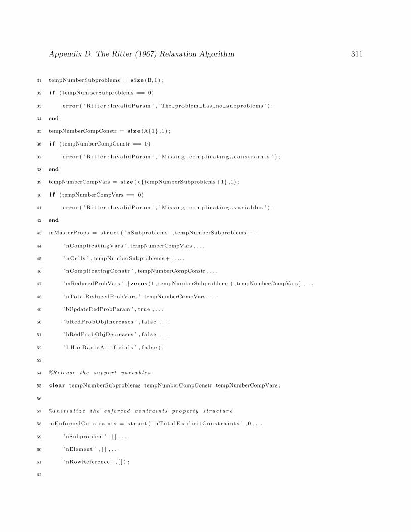
Appendix D. The Ritter (1967) Relaxation Algorithm 311
31 tempNumberSubproblems = s ize (B, 1 ) ;
32 i f ( tempNumberSubproblems == 0)
33 error ( ’ R i t t e r : InvalidParam ’ , ’The problem has no subproblems ’ ) ;
34 end
35 tempNumberCompConstr = s ize (A{1} , 1 ) ;
36 i f ( tempNumberCompConstr == 0)
37 error ( ’ R i t t e r : InvalidParam ’ , ’ Miss ing compl i ca t ing c o n s t r a i n t s ’ ) ;
38 end
39 tempNumberCompVars = s ize ( c{tempNumberSubproblems+1} ,1) ;
40 i f ( tempNumberCompVars == 0)
41 error ( ’ R i t t e r : InvalidParam ’ , ’ Miss ing compl i ca t ing v a r i a b l e s ’ ) ;
42 end
43 mMasterProps = s t r u c t ( ’ nSubproblems ’ , tempNumberSubproblems , . . .
44 ’ nComplicatingVars ’ , tempNumberCompVars , . . .
45 ’ nCe l l s ’ , tempNumberSubproblems + 1 , . . .
46 ’ nComplicatingConstr ’ , tempNumberCompConstr , . . .
47 ’ mReducedProbVars ’ , [ zeros (1 , tempNumberSubproblems ) , tempNumberCompVars ] , . . .
48 ’ nTotalReducedProbVars ’ , tempNumberCompVars , . . .
49 ’ bUpdateRedProbParam ’ , true , . . .
50 ’ bRedProbObjIncreases ’ , f a l s e , . . .
51 ’ bRedProbObjDecreases ’ , f a l s e , . . .
52 ’ b H a s B a s i c A r t i f i c i a l s ’ , f a l s e ) ;
53
54 %Release the support v a r i a b l e s
55 clear tempNumberSubproblems tempNumberCompConstr tempNumberCompVars ;
56
57 %I n i t i a l i z e the enforced con t ra in t s proper ty s t r u c t u r e
58 mEnforcedConstraints = s t r u c t ( ’ nTota lExp l i c i tCons t r a in t s ’ , 0 , . . .
59 ’ nSubproblem ’ , [ ] , . . .
60 ’ nElement ’ , [ ] , . . .
61 ’ nRowReference ’ , [ ] ) ;
62

Appendix D. The Ritter (1967) Relaxation Algorithm 312
63 %I n i t i a l i z e the re turn parameters proper ty s t r u c t u r e
64 sOutput = s t r u c t ( ’ x ’ , [ ] , . . .
65 ’ nObjValue ’ ,−Inf , . . .
66 ’ n I t e r a t i o n s ’ , 0 , . . .
67 ’ nSolutionTime ’ , clock , . . .
68 ’ sResu l t ’ , ’ ’ , . . .
69 ’ s D e s c r i p t i o n ’ , ’ ’ ) ;
70
71 %I n i t i a l i z e the subproblem proper ty s t r u c t u r e
72 mSubProps = c e l l ( mMasterProps . nSubproblems , 1 ) ;
73
74 %I n i t i a l i z e the subproblem element proper ty s t r u c t u r e
75 mElementProps = c e l l ( mMasterProps . nSubproblems , 1 ) ;
76
77 %I n i t i a l i z e the subproblem so l u t i on proper ty s t r u c t u r e
78 mSubSolProps = c e l l ( mMasterProps . nSubproblems , 1 ) ;
79
80 %I n i t i a l i z e the pa r t i t i o n ed submatr ices :
81 %va r i a b l e s with t h e i r non−n e g a t i v i t y r e s t r i c t i o n re l a xed −−> s e t 1 ;
82 %va r i a b l e s with t h e i r non−n e g a t i v i t y r e s t r i c t i o n enforced −−> s e t 2 ;
83 AA = c e l l ( mMasterProps . nSubproblems , 2 ) ;
84 BB = c e l l ( mMasterProps . nSubproblems , 2 ) ;
85 cc = c e l l ( mMasterProps . nSubproblems , 2 ) ;
86
87 %I n i t i a l i z e the reduced problem parameters
88 d = c e l l ( mMasterProps . nCel l s , 1 ) ;
89 F = c e l l (1 , mMasterProps . nCe l l s ) ;
90
91 %I n i t i a l i z e the reduced problem support parameters
92 iBB = c e l l ( mMasterProps . nSubproblems , 1 ) ;
93 iBb = c e l l ( mMasterProps . nSubproblems , 1 ) ;
94 iBD = c e l l ( mMasterProps . nSubproblems , 1 ) ;

Appendix D. The Ritter (1967) Relaxation Algorithm 313
95
96 %For each subproblem
97 for i = 1 : mMasterProps . nSubproblems
98
99 %Populate the i ˆ{ th } subproblem proper ty s t r u c t u r e
100 [ tempRows , tempCols ] = s ize (B{ i }) ;
101 t e m p A r t i f i c i a l = max(max( tempRows−tempCols +1 ,0) , tempRows−rank (B{ i }) ) ;
102 while ( t e m p A r t i f i c i a l <= tempRows)
103 i f (rank ( [B{ i } ,eye ( tempRows , t e m p A r t i f i c i a l ) ] ) == tempRows)
104 break ;
105 else
106 t e m p A r t i f i c i a l = t e m p A r t i f i c i a l +1;
107 end
108 end
109 mSubProps{ i } = s t r u c t ( ’ nRea lVar iab les ’ , tempCols , . . .
110 ’ n A r t i f i c i a l V a r i a b l e s ’ , t e m p A r t i f i c i a l , . . .
111 ’ nTota lVar iab le s ’ , tempCols+t e m p A r t i f i c i a l , . . .
112 ’ nConstra ints ’ , tempRows , . . .
113 ’ nVar iab le sSet1 ’ , tempRows , . . .
114 ’ nVar iab le sSet2 ’ , tempCols+t e m p A r t i f i c i a l−tempRows , . . .
115 ’ bUpdateRedProbParam ’ , true , . . .
116 ’ nNonNegCase ’ , 0 ) ;
117
118 %I n i t i a l i z e the i ˆ{ th } subproblem element proper ty s t r u c t u r e
119 tempData = zeros ( mSubProps{ i } . nTota lVar iables , 1 ) ;
120 mElementProps{ i } = s t r u c t ( ’ idxRe fe rence ’ , tempData , . . .
121 ’ bIsRelaxed ’ , boolean ( tempData ) , . . .
122 ’ b I s A r t i f i c i a l ’ , boolean ( tempData ) , . . .
123 ’ bEnforceNonNeg ’ , boolean ( tempData ) , . . .
124 ’ bSwapCol ’ , boolean ( tempData ) , . . .
125 ’ b I sEnforced ’ , boolean ( tempData ) ) ;
126

Appendix D. The Ritter (1967) Relaxation Algorithm 314
127 %I n i t i a l i z e the i ˆ{ th } subproblem so l u t i on proper ty s t r u c t u r e
128 mSubSolProps{ i } = s t r u c t ( ’ nNegative ’ , 0 , . . .
129 ’ idxNegat ives ’ , zeros ( mSubProps{ i } . nVar iab lesSet1 , 1 ) , . . .
130 ’ idxMostNeg ’ , 0 , . . .
131 ’ nMostNegativeValue ’ , Inf , . . .
132 ’ nPos i t i v e ’ , 0 , . . .
133 ’ i d x P o s i t i v e s ’ , zeros ( mSubProps{ i } . nVar iab lesSet2 , 1 ) ) ;
134
135 %Update the t o t a l number o f v a r i a b l e s in s e t 2
136 mMasterProps . mReducedProbVars ( i ) = mSubProps{ i } . nVar iab l e sSet2 ;
137 mMasterProps . nTotalReducedProbVars = . . .
138 mMasterProps . nTotalReducedProbVars+mSubProps{ i } . nVar iab l e sSet2 ;
139
140 i f mSubProps{ i } . n A r t i f i c i a l V a r i a b l e s > 0
141 %I f needed , augment the i ˆ{ th } subproblem A, B and c matr ices /
142 %vec to r s to ensure the ex i s t ance o f a non−s i n gu l a r matrix
143 B{ i } = [B{ i } ,eye ( mSubProps{ i } . nConstra ints , mSubProps{ i } . n A r t i f i c i a l V a r i a b l e s ) ] ;
144 c{ i } = [ c{ i } ; n In f ∗ ones ( mSubProps{ i } . n A r t i f i c i a l V a r i a b l e s , 1 ) ] ;
145 A{ i } = [A{ i } , . . .
146 zeros ( mMasterProps . nComplicatingConstr , mSubProps{ i } . n A r t i f i c i a l V a r i a b l e s ) ] ;
147
148 %Flag the crea ted v a r i a b l e s as a r t i f i c i a l
149 mElementProps{ i } . b I s A r t i f i c i a l ( mSubProps{ i } . . .
150 . nRea lVar iab les +1:mSubProps{ i } . nTota lVar iab le s ) = . . .
151 ones ( mSubProps{ i } . n A r t i f i c i a l V a r i a b l e s , 1 ) ;
152 end
153
154 %Id en f i f y a s t a r t i n g ba s i s
155 tempData = rref (B{ i }) ;
156 n1 = 0 ;
157 n2 = 0 ;
158

Appendix D. The Ritter (1967) Relaxation Algorithm 315
159 %For each element in the i ˆ{ th } subproblem
160 for j = 1 : mSubProps{ i } . nTota lVar iab le s
161
162 %Determine i f the v a r i a b l e be l ongs to s e t 1 or 2 ( i . e . , determine
163 %i f i t s non−n e g a t i v i t y r e s t r i c t i o n shou ld be r e l a xed or not )
164 i f ( n1 < mSubProps{ i } . nVar iab l e sSet1 )
165 mElementProps{ i } . bIsRelaxed ( j ) = boolean ( tempData ( n1+1, j ) == 1) ;
166 else
167 mElementProps{ i } . bIsRelaxed ( j ) = f a l s e ;
168 end
169
170 %Par t i t i on the i ˆ{ th } subproblem cons t r a in t s e t e lements in to the
171 %re laxed and non−r e l a xed s e t s
172 i f ( mElementProps{ i } . bIsRelaxed ( j ) )
173
174 %Add the v a r i a b l e to s e t 1
175 AA{ i , 1} = [AA{ i , 1} ,A{ i } ( : , j ) ] ;
176 BB{ i , 1} = [BB{ i , 1} ,B{ i } ( : , j ) ] ;
177 cc { i , 1} = [ cc { i , 1 } ; c{ i }( j ) ] ;
178
179 %Update counters
180 n1 = n1+1;
181 mElementProps{ i } . i dxRe fe rence ( j ) = n1 ;
182 else
183
184 %Add the v a r i a b l e to s e t 2
185 AA{ i , 2} = [AA{ i , 2} ,A{ i } ( : , j ) ] ;
186 BB{ i , 2} = [BB{ i , 2} ,B{ i } ( : , j ) ] ;
187 cc { i , 2} = [ cc { i , 2 } ; c{ i }( j ) ] ;
188
189 %Update counters
190 n2 = n2+1;
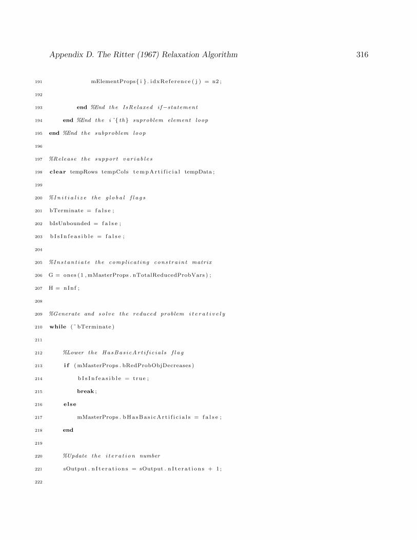
Appendix D. The Ritter (1967) Relaxation Algorithm 316
191 mElementProps{ i } . i dxRe fe rence ( j ) = n2 ;
192
193 end %End the IsRelaxed i f−s tatement
194 end %End the i ˆ{ th } suproblem element loop
195 end %End the subproblem loop
196
197 %Release the support v a r i a b l e s
198 clear tempRows tempCols t e m p A r t i f i c i a l tempData ;
199
200 %I n i t i a l i z e the g l o b a l f l a g s
201 bTerminate = f a l s e ;
202 bIsUnbounded = f a l s e ;
203 b I s I n f e a s i b l e = f a l s e ;
204
205 %In s t an t i a t e the comp l i ca t ing cons t r a in t matrix
206 G = ones (1 , mMasterProps . nTotalReducedProbVars ) ;
207 H = nInf ;
208
209 %Generate and s o l v e the reduced problem i t e r a t i v e l y
210 while (˜ bTerminate )
211
212 %Lower the HasBas i cAr t i f i c i a l s f l a g
213 i f ( mMasterProps . bRedProbObjDecreases )
214 b I s I n f e a s i b l e = true ;
215 break ;
216 else
217 mMasterProps . b H a s B a s i c A r t i f i c i a l s = f a l s e ;
218 end
219
220 %Update the i t e r a t i o n number
221 sOutput . n I t e r a t i o n s = sOutput . n I t e r a t i o n s + 1 ;
222
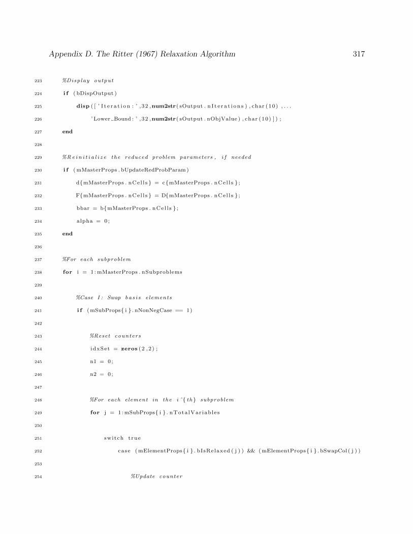
Appendix D. The Ritter (1967) Relaxation Algorithm 317
223 %Disp lay output
224 i f ( bDispOutput )
225 disp ( [ ’ I t e r a t i o n : ’ ,32 ,num2str( sOutput . n I t e r a t i o n s ) , char (10) , . . .
226 ’ Lower Bound : ’ ,32 ,num2str( sOutput . nObjValue ) , char (10) ] ) ;
227 end
228
229 %Re i n i t i a l i z e the reduced problem parameters , i f needed
230 i f ( mMasterProps . bUpdateRedProbParam )
231 d{mMasterProps . nCe l l s } = c{mMasterProps . nCe l l s } ;
232 F{mMasterProps . nCe l l s } = D{mMasterProps . nCe l l s } ;
233 bbar = b{mMasterProps . nCe l l s } ;
234 alpha = 0 ;
235 end
236
237 %For each subproblem
238 for i = 1 : mMasterProps . nSubproblems
239
240 %Case I : Swap ba s i s e lements
241 i f ( mSubProps{ i } . nNonNegCase == 1)
242
243 %Reset counters
244 idxSet = zeros ( 2 , 2 ) ;
245 n1 = 0 ;
246 n2 = 0 ;
247
248 %For each element in the i ˆ{ th } subproblem
249 for j = 1 : mSubProps{ i } . nTota lVar iab le s
250
251 switch true
252 case ( mElementProps{ i } . bIsRelaxed ( j ) ) && ( mElementProps{ i } . bSwapCol ( j ) )
253
254 %Update counter

Appendix D. The Ritter (1967) Relaxation Algorithm 318
255 n2 = n2+1;
256
257 %Save the current and de s t i na t i on column re f e r ence s
258 idxSet (1 , 1 ) = mElementProps{ i } . i dxRe fe rence ( j ) ;
259 idxSet (1 , 2 ) = n2 ;
260
261 %Update the remaining f l a g s
262 mElementProps{ i } . i dxRe fe rence ( j ) = n2 ;
263 mElementProps{ i } . bIsRelaxed ( j ) = f a l s e ;
264 mElementProps{ i } . bSwapCol ( j ) = f a l s e ;
265
266 case (˜ mElementProps{ i } . bIsRelaxed ( j ) ) && . . .
267 ( mElementProps{ i } . bSwapCol ( j ) )
268
269 %Update counter
270 n1 = n1+1;
271
272 %Save the current and de s t i na t i on column re f e r ence s
273 idxSet (2 , 1 ) = mElementProps{ i } . i dxRe fe rence ( j ) ;
274 idxSet (2 , 2 ) = n1 ;
275
276 %Update the remaining f l a g s
277 mElementProps{ i } . i dxRe fe rence ( j ) = n1 ;
278 mElementProps{ i } . bIsRelaxed ( j ) = true ;
279 mElementProps{ i } . bSwapCol ( j ) = f a l s e ;
280
281 case ( mElementProps{ i } . bIsRelaxed ( j ) ) && . . .
282 (˜ mElementProps{ i } . bSwapCol ( j ) )
283
284 %Update counter
285 n1 = n1+1;
286
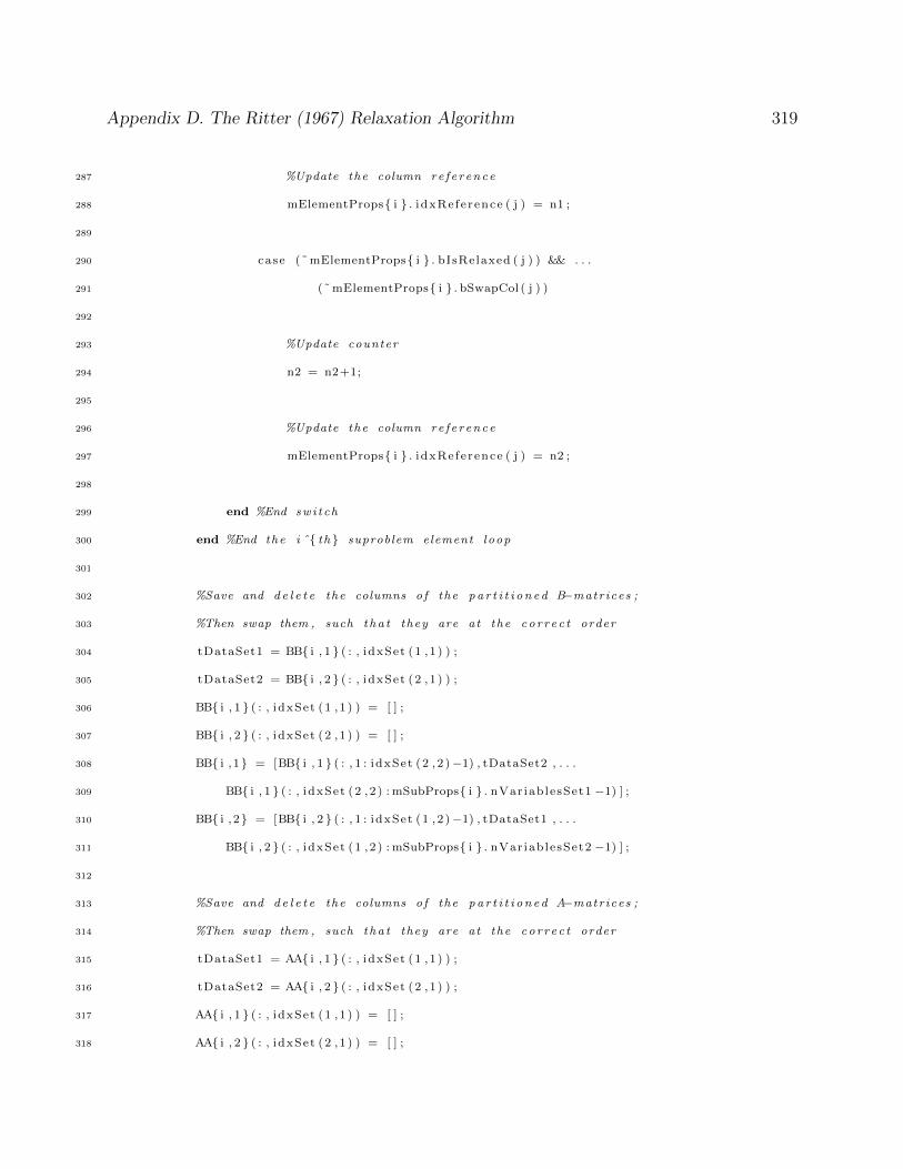
Appendix D. The Ritter (1967) Relaxation Algorithm 319
287 %Update the column re f e r ence
288 mElementProps{ i } . i dxRe fe rence ( j ) = n1 ;
289
290 case (˜ mElementProps{ i } . bIsRelaxed ( j ) ) && . . .
291 (˜ mElementProps{ i } . bSwapCol ( j ) )
292
293 %Update counter
294 n2 = n2+1;
295
296 %Update the column re f e r ence
297 mElementProps{ i } . i dxRe fe rence ( j ) = n2 ;
298
299 end %End swi tch
300 end %End the i ˆ{ th } suproblem element loop
301
302 %Save and d e l e t e the columns o f the pa r t i t i o n ed B−matrices ;
303 %Then swap them , such tha t they are at the co r r ec t order
304 tDataSet1 = BB{ i , 1 } ( : , idxSet (1 , 1 ) ) ;
305 tDataSet2 = BB{ i , 2 } ( : , idxSet (2 , 1 ) ) ;
306 BB{ i , 1 } ( : , idxSet (1 , 1 ) ) = [ ] ;
307 BB{ i , 2 } ( : , idxSet (2 , 1 ) ) = [ ] ;
308 BB{ i , 1} = [BB{ i , 1 } ( : , 1 : idxSet (2 , 2 )−1) , tDataSet2 , . . .
309 BB{ i , 1 } ( : , idxSet (2 , 2 ) : mSubProps{ i } . nVar iab lesSet1 −1) ] ;
310 BB{ i , 2} = [BB{ i , 2 } ( : , 1 : idxSet (1 , 2 )−1) , tDataSet1 , . . .
311 BB{ i , 2 } ( : , idxSet (1 , 2 ) : mSubProps{ i } . nVar iab lesSet2 −1) ] ;
312
313 %Save and d e l e t e the columns o f the pa r t i t i o n ed A−matrices ;
314 %Then swap them , such tha t they are at the co r r ec t order
315 tDataSet1 = AA{ i , 1 } ( : , idxSet (1 , 1 ) ) ;
316 tDataSet2 = AA{ i , 2 } ( : , idxSet (2 , 1 ) ) ;
317 AA{ i , 1 } ( : , idxSet (1 , 1 ) ) = [ ] ;
318 AA{ i , 2 } ( : , idxSet (2 , 1 ) ) = [ ] ;
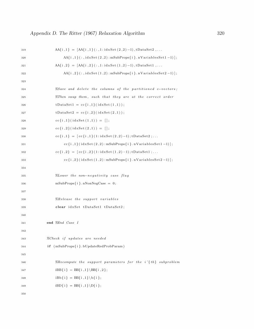
Appendix D. The Ritter (1967) Relaxation Algorithm 320
319 AA{ i , 1} = [AA{ i , 1 } ( : , 1 : idxSet (2 , 2 )−1) , tDataSet2 , . . .
320 AA{ i , 1 } ( : , idxSet (2 , 2 ) : mSubProps{ i } . nVar iab lesSet1 −1) ] ;
321 AA{ i , 2} = [AA{ i , 2 } ( : , 1 : idxSet (1 , 2 )−1) , tDataSet1 , . . .
322 AA{ i , 2 } ( : , idxSet (1 , 2 ) : mSubProps{ i } . nVar iab lesSet2 −1) ] ;
323
324 %Save and d e l e t e the columns o f the pa r t i t i o n ed c−vec t o r s ;
325 %Then swap them , such tha t they are at the co r r ec t order
326 tDataSet1 = cc { i , 1} ( idxSet (1 , 1 ) ) ;
327 tDataSet2 = cc { i , 2} ( idxSet (2 , 1 ) ) ;
328 cc { i , 1} ( idxSet (1 , 1 ) ) = [ ] ;
329 cc { i , 2} ( idxSet (2 , 1 ) ) = [ ] ;
330 cc { i , 1} = [ cc { i , 1 } ( 1 : idxSet (2 , 2 )−1) ; tDataSet2 ; . . .
331 cc { i , 1} ( idxSet (2 , 2 ) : mSubProps{ i } . nVar iab lesSet1 −1) ] ;
332 cc { i , 2} = [ cc { i , 2 } ( 1 : idxSet (1 , 2 )−1) ; tDataSet1 ; . . .
333 cc { i , 2} ( idxSet (1 , 2 ) : mSubProps{ i } . nVar iab lesSet2 −1) ] ;
334
335 %Lower the non−n e g a t i v i t y case f l a g
336 mSubProps{ i } . nNonNegCase = 0 ;
337
338 %Release the support v a r i a b l e s
339 clear idxSet tDataSet1 tDataSet2 ;
340
341 end %End Case I
342
343 %Check i f updates are needed
344 i f ( mSubProps{ i } . bUpdateRedProbParam )
345
346 %Recompute the support parameters f o r the i ˆ{ th } subproblem
347 iBB{ i } = BB{ i , 1}\BB{ i , 2 } ;
348 iBb{ i } = BB{ i , 1}\b{ i } ;
349 iBD{ i } = BB{ i , 1}\D{ i } ;
350
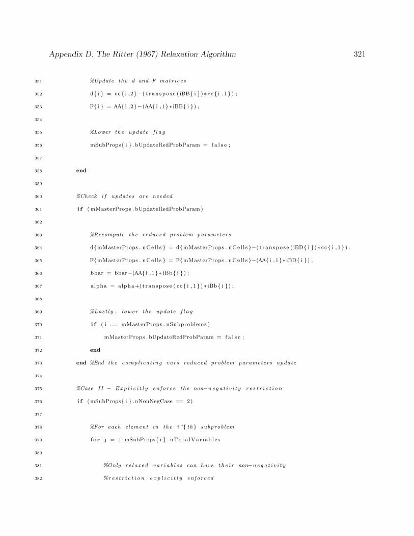
Appendix D. The Ritter (1967) Relaxation Algorithm 321
351 %Update the d and F matr ices
352 d{ i } = cc { i ,2}−( t ranspose ( iBB{ i }) ∗ cc { i , 1} ) ;
353 F{ i } = AA{ i ,2}−(AA{ i , 1}∗ iBB{ i }) ;
354
355 %Lower the update f l a g
356 mSubProps{ i } . bUpdateRedProbParam = f a l s e ;
357
358 end
359
360 %Check i f updates are needed
361 i f ( mMasterProps . bUpdateRedProbParam )
362
363 %Recompute the reduced problem parameters
364 d{mMasterProps . nCe l l s } = d{mMasterProps . nCe l l s }−( t ranspose ( iBD{ i }) ∗ cc { i , 1} ) ;
365 F{mMasterProps . nCe l l s } = F{mMasterProps . nCe l l s }−(AA{ i , 1}∗ iBD{ i }) ;
366 bbar = bbar−(AA{ i , 1}∗ iBb{ i }) ;
367 alpha = alpha+( t ranspose ( cc { i , 1} ) ∗ iBb{ i }) ;
368
369 %Last ly , lower the update f l a g
370 i f ( i == mMasterProps . nSubproblems )
371 mMasterProps . bUpdateRedProbParam = f a l s e ;
372 end
373 end %End the comp l i ca t ing vars reduced problem parameters update
374
375 %Case I I − E x p l i c i t l y en force the non−n e g a t i v i t y r e s t r i c t i o n
376 i f ( mSubProps{ i } . nNonNegCase == 2)
377
378 %For each element in the i ˆ{ th } subproblem
379 for j = 1 : mSubProps{ i } . nTota lVar iab le s
380
381 %Only re l a xed v a r i a b l e s can have t h e i r non−n e g a t i v i t y
382 %r e s t r i c t i o n e x p l i c i t l y enforced
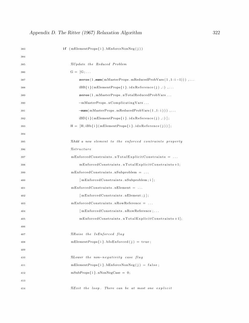
Appendix D. The Ritter (1967) Relaxation Algorithm 322
383 i f ( mElementProps{ i } . bEnforceNonNeg ( j ) )
384
385 %Update the Reduced Problem
386 G = [G ; . . .
387 zeros (1 ,sum( mMasterProps . mReducedProbVars ( 1 , 1 : i −1) ) ) , . . .
388 iBB{ i }( mElementProps{ i } . i dxRe fe rence ( j ) , : ) , . . .
389 zeros (1 , mMasterProps . nTotalReducedProbVars . . .
390 −mMasterProps . nComplicatingVars . . .
391 −sum( mMasterProps . mReducedProbVars ( 1 , 1 : i ) ) ) , . . .
392 iBD{ i }( mElementProps{ i } . i dxRe fe rence ( j ) , : ) ] ;
393 H = [H; iBb{ i }( mElementProps{ i } . i dxRe fe rence ( j ) ) ] ;
394
395 %Add a new element to the enforced con t ra in t s proper ty
396 %s t ru c t u r e
397 mEnforcedConstraints . nTota lExp l i c i tCons t r a in t s = . . .
398 mEnforcedConstraints . nTota lExp l i c i tCons t r a in t s +1;
399 mEnforcedConstraints . nSubproblem = . . .
400 [ mEnforcedConstraints . nSubproblem ; i ] ;
401 mEnforcedConstraints . nElement = . . .
402 [ mEnforcedConstraints . nElement ; j ] ;
403 mEnforcedConstraints . nRowReference = . . .
404 [ mEnforcedConstraints . nRowReference ; . . .
405 mEnforcedConstraints . nTota lExp l i c i tCons t r a in t s +1] ;
406
407 %Raise the IsEnforced f l a g
408 mElementProps{ i } . b I sEnforced ( j ) = true ;
409
410 %Lower the non−n e g a t i v i t y case f l a g
411 mElementProps{ i } . bEnforceNonNeg ( j ) = f a l s e ;
412 mSubProps{ i } . nNonNegCase = 0 ;
413
414 %Exi t the loop . There can be at most one e x p l i c i t
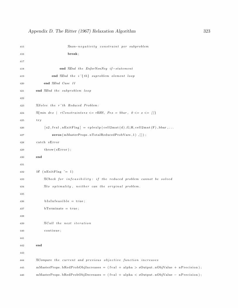
Appendix D. The Ritter (1967) Relaxation Algorithm 323
415 %non−n e g a t i v i t y con s t r a in t per subproblem
416 break ;
417
418 end %End the EnforNonNeg i f−s tatement
419 end %End the i ˆ{ th } suproblem element loop
420 end %End Case I I
421 end %End the subproblem loop
422
423 %Solve the rˆ th Reduced Problem :
424 %{min d∗x | rCons t ra in t s ∗x <= rRHS, F∗x = bbar , 0 <= x <= [ ] }
425 t ry
426 [ x2 , f va l , nExitFlag ] = c p l e x l p ( ce l l 2mat (d) ,G,H, ce l l 2mat (F) , bbar , . . .
427 zeros ( mMasterProps . nTotalReducedProbVars , 1 ) , [ ] ) ;
428 catch sError
429 throw ( sError ) ;
430 end
431
432 i f ( nExitFlag ˜= 1)
433 %Check f o r i n f e a s i b i l i t y : i f the reduced problem cannot be so l v ed
434 %to op t ima l i t y , ne i t h e r can the o r i g i n a l problem .
435
436 b I s I n f e a s i b l e = true ;
437 bTerminate = true ;
438
439 %Cal l the next i t e r a t i o n
440 cont inue ;
441
442 end
443
444 %Compare the current and prev ious o b j e c t i v e func t i on inc rea se s
445 mMasterProps . bRedProbObjIncreases = ( f v a l + alpha > sOutput . nObjValue + nPrec i s i on ) ;
446 mMasterProps . bRedProbObjDecreases = ( f v a l + alpha < sOutput . nObjValue − nPrec i s i on ) ;
Appendix D. The Ritter (1967) Relaxation Algorithm 324
447
448 %Save the new o b j e c t i v e func t i on va lue
449 sOutput . nObjValue = f v a l+alpha ;
450
451 %Check i f the unboundedness cons t r a in t i s b ind ing
452 bIsUnbounded = (sum( x2 ) > nIn f − nPrec i s i on ) ;
453
454 %Parse the r e s u l t s o f the op t imi za t i on problem in to c e l l s according
455 %to the number o f v a r i a b l e s in the reduced problem
456 x1 = c e l l ( mMasterProps . nSubproblems , 1 ) ;
457 x2 = mat2ce l l ( x2 , mMasterProps . mReducedProbVars , 1 ) ;
458
459 %Raise the terminat ion f l a g . I t may have to be lowered again l a t e r
460 bTerminate = true ;
461
462 %For each subproblem
463 for i = 1 : mMasterProps . nSubproblems
464
465 %Compute the s o l u t i on to the r e l a xed v a r i a b l e s
466 x1{ i } = iBb{ i }−(iBB{ i }∗x2{ i })−(iBD{ i }∗x2{mMasterProps . nCe l l s }) ;
467
468 %For each element in the subproblem
469 for j = 1 : mSubProps{ i } . nTota lVar iab le s
470
471 %Determine i f t he re are any ba s i c a r t i f i c i a l v a r i a b l e s
472 i f ( mElementProps{ i } . b I s A r t i f i c i a l ( j ) )
473 i f ( ( mElementProps{ i } . bIsRelaxed ( j ) ) && . . .
474 ( x1{ i }( mElementProps{ i } . i dxRe fe rence ( j ) ) > nPrec i s i on ) ) | | . . .
475 ( (˜ mElementProps{ i } . bIsRelaxed ( j ) ) && . . .
476 ( x2{ i }( mElementProps{ i } . i dxRe fe rence ( j ) ) > nPrec i s i on ) )
477
478 %Raise the HasBas i cAr t i f i c i a l sF l a g
Appendix D. The Ritter (1967) Relaxation Algorithm 325
479 mMasterProps . b H a s B a s i c A r t i f i c i a l s = true ;
480 end
481 end
482
483 i f ( mElementProps{ i } . bIsRelaxed ( j ) )
484
485 %I f the r e l a xed dec i s i on v a r i a b l e i s negat ive , add
486 %i t to the nega t i v e l i s t
487 i f ( x1{ i }( mElementProps{ i } . i dxRe fe rence ( j ) ) < −nPrec i s i on )
488
489 %Not a l l non−n e g a t i v i t y r e s t r i c t i o n s were s a t i s f i e d
490 %Lower the terminat ion f l a g
491 bTerminate = f a l s e ;
492
493 %Add the v a r i a b l e to the nega t i v e l i s t
494 mSubSolProps{ i } . nNegative = mSubSolProps{ i } . nNegative +1;
495 mSubSolProps{ i } . idxNegat ives ( mSubSolProps{ i } . nNegative ) = j ;
496
497 %Update the most nega t i v e v a r i a b l e found so fa r .
498 i f ( x1{ i }( mElementProps{ i } . i dxRe fe rence ( j ) ) < . . .
499 mSubSolProps{ i } . nMostNegativeValue )
500 mSubSolProps{ i } . idxMostNeg = j ;
501 mSubSolProps{ i } . nMostNegativeValue = . . .
502 x1{ i }( mElementProps{ i } . i dxRe fe rence ( j ) ) ;
503 end
504 end %End IsRelaxed && IsNega t i ve i f−s tatement
505
506 else
507 %I f the reduced problem dec i s i on v a r i a b l e i s p o s i t i v e ,
508 %add i t to the p o s i t i v e l i s t
509 i f ( x2{ i }( mElementProps{ i } . i dxRe fe rence ( j ) ) > nPrec i s i on )
510 mSubSolProps{ i } . nPos i t i v e = mSubSolProps{ i } . nPos i t i v e +1;
Appendix D. The Ritter (1967) Relaxation Algorithm 326
511 mSubSolProps{ i } . i d x P o s i t i v e s ( mSubSolProps{ i } . nPos i t i v e ) = j ;
512 end
513
514 end %End the ˜ IsRe laxed && ˜ IsNega t i ve i f−s tatement
515 end %End the i ˆ{ th } subproblem element loop
516
517 %Remove unused row elements from the l i s t s to c l e a r memory
518 mSubSolProps{ i } . idxNegat ives ( mSubSolProps{ i } . nNegative +1:end) = [ ] ;
519 mSubSolProps{ i } . i d x P o s i t i v e s ( mSubSolProps{ i } . nPos i t i v e +1:end) = [ ] ;
520
521 end %End the subproblem loop
522
523 %Deal with the e x p l i c i t non−n e g a t i v i t y c on s t r a i n t s
524 i f ( mMasterProps . bRedProbObjIncreases && . . .
525 ( mEnforcedConstraints . nTota lExp l i c i tCons t r a in t s > 0) )
526
527 %Reset counter
528 z1 = 0 ;
529
530 %For each enforced cons t r a in t
531 while ( z1 < mEnforcedConstraints . nTota lExp l i c i tCons t r a in t s )
532
533 %Increment counter
534 z1 = z1 +1;
535
536 %Lower the support f l a g s
537 bAllowRemoval = f a l s e ;
538
539 i f ( mElementProps{mEnforcedConstraints . nSubproblem ( z1 ) } . . . .
540 bIsRelaxed ( mEnforcedConstraints . nElement ( z1 ) ) )
541
542 %Save the re f e r ence to the kˆ{ th } row
Appendix D. The Ritter (1967) Relaxation Algorithm 327
543 n1 = mElementProps{mEnforcedConstraints . nSubproblem ( z1 ) } . . .
544 . i dxRe fe rence ( mEnforcedConstraints . nElement ( z1 ) ) ;
545
546 i f ( x1{mEnforcedConstraints . nSubproblem ( z1 ) }( n1 ) > nPrec i s i on )
547 %CASE 3: Raise the removal f l a g i f the e x p l i c i t
548 %non−n e g a t i v i t y r e s t r i c t i o n i s non−b ind ing
549 bAllowRemoval = true ;
550
551 e l s e i f ( mSubProps{mEnforcedConstraints . nSubproblem ( z1 ) } . nNonNegCase == 0) ;
552 %CASE 4: The r e s t r i c t i o n i s b ind ing . Scan the
553 %reduced problem so l u t i on fo r a p o t e n t i a l e lement
554 %to l eave the b a s i s so t ha t t h i s one may enter
555
556 %Loop through a l l e lements again
557 for n = 1 : mSubProps{mEnforcedConstraints . . .
558 . nSubproblem ( z1 ) } . nTota lVar iab le s
559 i f (˜ mElementProps{mEnforcedConstraints . . .
560 . nSubproblem ( z1 ) } . bIsRelaxed (n) )
561
562 %Save the re f e r ence to the qˆ{ th } column
563 n2 = mElementProps{mEnforcedConstraints . nSubproblem ( z1 ) } . . .
564 . i dxRe fe rence (n) ;
565
566 %I f we f ind a p o s i t i v e element in s e t 1
567 %which w i l l not l ead to a s i n gu l a r matrix
568 i f ( x2{mEnforcedConstraints . nSubproblem ( z1 ) }( n2 ) . . .
569 > nPrec i s i on ) && ( ( iBB{mEnforcedConstraints . . .
570 . nSubproblem ( z1 ) }( n1 , n2 ) < −nPrec i s i on ) | | . . .
571 ( iBB{mEnforcedConstraints . nSubproblem ( z1 ) }( n1 , n2 ) . . .
572 > nPrec i s i on ) )
573
574 %Raise the r e s p e c t i v e swap ba s i s f l a g s
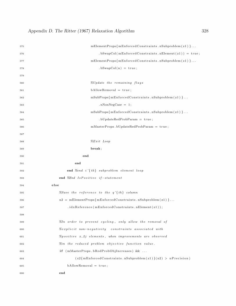
Appendix D. The Ritter (1967) Relaxation Algorithm 328
575 mElementProps{mEnforcedConstraints . nSubproblem ( z1 ) } . . .
576 . bSwapCol ( mEnforcedConstraints . nElement ( z1 ) ) = true ;
577 mElementProps{mEnforcedConstraints . nSubproblem ( z1 ) } . . .
578 . bSwapCol (n) = true ;
579
580 %Update the remaining f l a g s
581 bAllowRemoval = true ;
582 mSubProps{mEnforcedConstraints . nSubproblem ( z1 ) } . . .
583 . nNonNegCase = 1 ;
584 mSubProps{mEnforcedConstraints . nSubproblem ( z1 ) } . . .
585 . bUpdateRedProbParam = true ;
586 mMasterProps . bUpdateRedProbParam = true ;
587
588 %Exi t Loop
589 break ;
590 end
591 end
592 end %end i ˆ{ th } subproblem element loop
593 end %End I sPo s i t i v e i f−s tatement
594 else
595 %Save the re f e r ence to the qˆ{ th } column
596 n2 = mElementProps{mEnforcedConstraints . nSubproblem ( z1 ) } . . .
597 . i dxRe fe rence ( mEnforcedConstraints . nElement ( z1 ) ) ;
598
599 %In order to prevent cyc l ing , only a l l ow the removal o f
600 %e x p l i c i t non−n e g a t i v i t y c on s t r a i n t s a s soc i a t ed with
601 %po s i t i v e x 2 j elements , when improvements are observed
602 %in the reduced problem o b j e c t i v e func t i on va lue .
603 i f ( mMasterProps . bRedProbObjIncreases ) && . . .
604 ( x2{mEnforcedConstraints . nSubproblem ( z1 ) }( n2 ) > nPrec i s i on )
605 bAllowRemoval = true ;
606 end
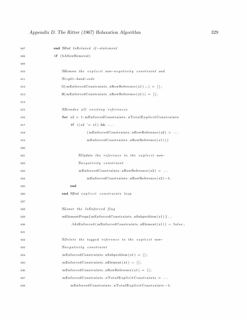
Appendix D. The Ritter (1967) Relaxation Algorithm 329
607 end %End IsRelaxed i f−s tatement
608 i f ( bAllowRemoval )
609
610 %Remove the e x p l i c i t non−n e g a t i v i t y con s t r a in t and
611 %righ t−hand−s i d e
612 G( mEnforcedConstraints . nRowReference ( z1 ) , : ) = [ ] ;
613 H( mEnforcedConstraints . nRowReference ( z1 ) ) = [ ] ;
614
615 %Reindex a l l e x i s t i n g r e f e r ence s
616 for z2 = 1 : mEnforcedConstraints . nTota lExp l i c i tCons t r a in t s
617 i f ( ( z2 ˜= z1 ) && . . .
618 ( mEnforcedConstraints . nRowReference ( z2 ) > . . .
619 mEnforcedConstraints . nRowReference ( z1 ) ) )
620
621 %Update the re f e r ence to the e x p l i c i t non−
622 %ne g a t i v i t y con s t r a in t
623 mEnforcedConstraints . nRowReference ( z2 ) = . . .
624 mEnforcedConstraints . nRowReference ( z2 )−1;
625 end
626 end %End e x p l i c i t c on s t r a i n t s loop
627
628 %Lower the IsEnforced f l a g
629 mElementProps{mEnforcedConstraints . nSubproblem ( z1 ) } . . .
630 . b I sEnforced ( mEnforcedConstraints . nElement ( z1 ) ) = f a l s e ;
631
632 %Dele te the tagged re f e r ence to the e x p l i c i t non−
633 %ne g a t i v i t y con s t r a in t
634 mEnforcedConstraints . nSubproblem ( z1 ) = [ ] ;
635 mEnforcedConstraints . nElement ( z1 ) = [ ] ;
636 mEnforcedConstraints . nRowReference ( z1 ) = [ ] ;
637 mEnforcedConstraints . nTota lExp l i c i tCons t r a in t s = . . .
638 mEnforcedConstraints . nTota lExp l i c i tCons t ra in t s −1;
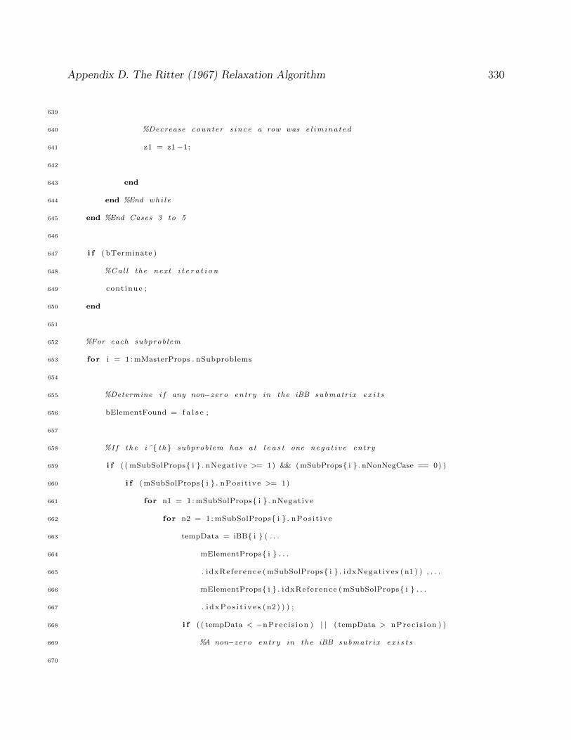
Appendix D. The Ritter (1967) Relaxation Algorithm 330
639
640 %Decrease counter s ince a row was e l imina ted
641 z1 = z1−1;
642
643 end
644 end %End whi l e
645 end %End Cases 3 to 5
646
647 i f ( bTerminate )
648 %Cal l the next i t e r a t i o n
649 cont inue ;
650 end
651
652 %For each subproblem
653 for i = 1 : mMasterProps . nSubproblems
654
655 %Determine i f any non−zero entry in the iBB submatrix e x i t s
656 bElementFound = f a l s e ;
657
658 %I f the i ˆ{ th } subproblem has at l e a s t one nega t i v e entry
659 i f ( ( mSubSolProps{ i } . nNegative >= 1) && ( mSubProps{ i } . nNonNegCase == 0) )
660 i f ( mSubSolProps{ i } . nPos i t i v e >= 1)
661 for n1 = 1 : mSubSolProps{ i } . nNegative
662 for n2 = 1 : mSubSolProps{ i } . nPos i t i v e
663 tempData = iBB{ i } ( . . .
664 mElementProps{ i } . . .
665 . i dxRe fe rence ( mSubSolProps{ i } . idxNegat ives ( n1 ) ) , . . .
666 mElementProps{ i } . i dxRe fe rence ( mSubSolProps{ i } . . .
667 . i d x P o s i t i v e s ( n2 ) ) ) ;
668 i f ( ( tempData < −nPrec i s i on ) | | ( tempData > nPrec i s i on ) )
669 %A non−zero entry in the iBB submatrix e x i s t s
670
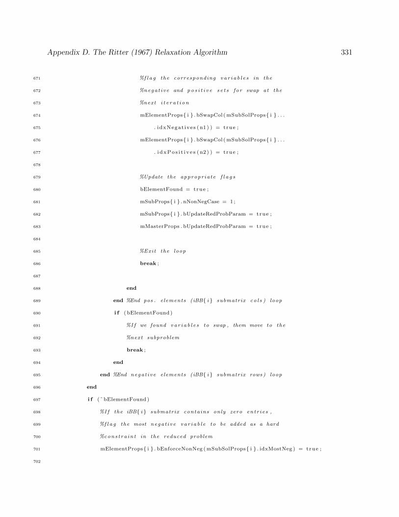
Appendix D. The Ritter (1967) Relaxation Algorithm 331
671 %f l a g the corresponding v a r i a b l e s in the
672 %nega t i v e and p o s i t i v e s e t s f o r swap at the
673 %next i t e r a t i o n
674 mElementProps{ i } . bSwapCol ( mSubSolProps{ i } . . .
675 . idxNegat ives ( n1 ) ) = true ;
676 mElementProps{ i } . bSwapCol ( mSubSolProps{ i } . . .
677 . i d x P o s i t i v e s ( n2 ) ) = true ;
678
679 %Update the appropr ia t e f l a g s
680 bElementFound = true ;
681 mSubProps{ i } . nNonNegCase = 1 ;
682 mSubProps{ i } . bUpdateRedProbParam = true ;
683 mMasterProps . bUpdateRedProbParam = true ;
684
685 %Exi t the loop
686 break ;
687
688 end
689 end %End pos . e lements ( iBB{ i } submatrix c o l s ) loop
690 i f ( bElementFound )
691 %I f we found v a r i a b l e s to swap , them move to the
692 %next subproblem
693 break ;
694 end
695 end %End nega t i v e e lements ( iBB{ i } submatrix rows ) loop
696 end
697 i f (˜ bElementFound )
698 %I f the iBB{ i } submatrix conta ins only zero en t r i e s ,
699 %f l a g the most nega t i v e v a r i a b l e to be added as a hard
700 %cons t r a in t in the reduced problem
701 mElementProps{ i } . bEnforceNonNeg ( mSubSolProps{ i } . idxMostNeg ) = true ;
702
Appendix D. The Ritter (1967) Relaxation Algorithm 332
703 %Update the appropr ia t e f l a g s
704 mSubProps{ i } . nNonNegCase = 2 ;
705
706 end %End most nega t i v e i f−s tatement
707 end %End has nega t i v e e lements i f−s tatement
708
709 %Reset the number o f nega t i v e and p o s i t i v e va lue s counters
710 mSubSolProps{ i } . nNegative = 0 ;
711 mSubSolProps{ i } . idxNegat ives = zeros ( mSubProps{ i } . nVar iab lesSet1 , 1 ) ;
712 mSubSolProps{ i } . idxMostNeg = 0 ;
713 mSubSolProps{ i } . nMostNegativeValue = Inf ;
714 mSubSolProps{ i } . nPos i t i v e = 0 ;
715 mSubSolProps{ i } . i d x P o s i t i v e s = zeros ( mSubProps{ i } . nVar iab lesSet2 , 1 ) ;
716
717 end %End subproblem loop
718 end %End main wh i l e loop
719
720 %Release the support v a r i a b l e s
721 clear bTerminate bDispOutput mSubSolProps mEnforcedConstraints nIn f n1 n2 . . .
722 nPrec i s i on AA BB cc iBB iBb iBD G H d F bbar alpha nExitFlag f v a l . . .
723 z1 z2 nSubproblem bAllowRemoval bElementFound tempData n ;
724
725 %Output Resu l t s
726 switch true
727 case ( bIsUnbounded ) && (˜ b I s I n f e a s i b l e )
728 sOutput . sResu l t = ’ unbounded ’ ;
729 sOutput . s D e s c r i p t i o n = ’The o r i g i n a l problem i s unbounded ’ ;
730
731 case ( b I s I n f e a s i b l e | | mMasterProps . b H a s B a s i c A r t i f i c i a l s )
732 sOutput . sResu l t = ’ i n f e a s i b l e ’ ;
733 sOutput . s D e s c r i p t i o n = ’The o r i g i n a l problem i s i n f e a s i b l e ’ ;
734
Appendix D. The Ritter (1967) Relaxation Algorithm 333
735 otherw i se
736 sOutput . sResu l t = ’ optimal ’ ;
737 sOutput . s D e s c r i p t i o n = ’ Program Fin i shed . Optimal s o l u t i o n found ’ ;
738
739 %Output the f i n a l s o l u t i on
740 sOutput . x = c e l l ( mMasterProps . nCel l s , 1 ) ;
741
742 %For each subproblem
743 for i = 1 : mMasterProps . nSubproblems
744
745 %In s t an t i a t e the s o l u t i on s e t
746 sOutput . x{ i } = zeros ( mSubProps{ i } . nRealVar iables , 1 ) ;
747
748 %For each element in the i ˆ{ th } subproblem
749 n = 0 ;
750 for j = 1 : mSubProps{ i } . nTota lVar iab le s
751
752 i f (˜ mElementProps{ i } . b I s A r t i f i c i a l ( j ) )
753
754 %Update counter
755 n = n + 1 ;
756
757 %Merge the r e l a xed and non−r e l a xed s e t s
758 i f ( mElementProps{ i } . bIsRelaxed ( j ) )
759 sOutput . x{ i }(n) = x1{ i }( mElementProps{ i } . i dxRe fe rence ( j ) ) ;
760 else
761 sOutput . x{ i }(n) = x2{ i }( mElementProps{ i } . i dxRe fe rence ( j ) ) ;
762 end
763
764 end %End I s A r t i f i c i a l i f−s tatement
765 end %End the i ˆ{ th } subproblem element loop
766 end %End the subproblem loop

Appendix D. The Ritter (1967) Relaxation Algorithm 334
767
768 %Inc lude f i n a l va lue o f comp l i ca t ing v a r i a b l e s
769 sOutput . x{mMasterProps . nCel l s , 1} = x2{mMasterProps . nCel l s , 1 } ;
770
771 end %End swi tch
772
773 %Compute the e l apsed time
774 sOutput . nSolutionTime = etime ( clock , sOutput . nSolutionTime ) ;
775
776 %Release the remaining support v a r i a b l e s
777 clear i j x1 x2 b I s I n f e a s i b l e bIsUnbounded mMasterProps mSubProps . . .
778 mElementProps ;
779 end

Appendix D. The Ritter (1967) Relaxation Algorithm 335
D.2 Modified Algorithm
1 %%%%%%%%%%%%%%%%%%%%%%%%%%%%%%%%%%%%%%%%%%%%%%%%%%%%%%%%%%%%%%%%%%%%%%%%%%%
2 % This func t i on s o l v e s problems o f the type : %
3 % Min 0.5 x ’ H x + c ’ x %
4 % S . t . B{1}∗ x{1} + D{1}∗ x{p+1} == b{1} %
5 % B{2}∗ x{2} + + D{2}∗ x{p+1} == b{2} %
6 % . . . %
7 % B{p}∗x{p} + D{p}∗x{p+1} == b{p} %
8 % Aeq{1}∗ x{1} + . . . + Aeq{p}∗x{p} + Deq∗x{p+1} == beq %
9 % Aineq {1}∗ x{1} + . . . + Aineq{p}∗x{p} + Dineq∗x{p+1} <= bineq %
10 % x {1} , x {2} , . . . , x{p} , x{p+1} in (R + \ t imes Z +) %
11 %%%%%%%%%%%%%%%%%%%%%%%%%%%%%%%%%%%%%%%%%%%%%%%%%%%%%%%%%%%%%%%%%%%%%%%%%%%
12 % Input Parameters : %
13 % H{ i j } − a n j x n k matrix o f 2nd−order p a r t i a l d e r i v s . , i , j = 1 . . p+1 %
14 % c{ i } − a n{ i}−column vec tor o f ob j . func . c o e f f i c i e n t s , i = 1 , . . . , p+1 %
15 % Aeq{ i } − a m eq x n{ i } matrix o f con s t r a in t c o e f f i c i e n t s , i = 1 , . . . , p %
16 % Aineq{ i } − a m ineq x n{ i } matrix o f cons t r . c o e f f i c i e n t s , i = 1 , . . . , p %
17 % B{ i } − a m{ i } x n{ i } matrix o f con s t r a in t c o e f f i c i e n t s , i = 1 , . . . , p %
18 % D{ i } − a m{ i } x n{p+1} matrix o f con s t r a in t c o e f f i c i e n t s , i = 1 , . . . , p %
19 % Deq − a m eq x n{p+1} matrix o f con s t r a in t c o e f f i c i e n t s %
20 % Dineq − a m ineq x n{p+1} matrix o f con s t r a in t c o e f f i c i e n t s %
21 % b{ i } − a m{ i}−column vec tor o f RHS c o e f f i c i e n t s , i = 1 , . . . , p %
22 % beq − a m eq−column vec tor o f RHS c o e f f i c i e n t s %
23 % bineq − a m ineq−column vec tor o f RHS c o e f f i c i e n t s %
24 % %
25 % Output Paramters : %
26 % x{ i } − a n{ i}−column vec tor o f dec i s i on va r i a b l e s , i = 1 , . . . , p+1 %
27 % f v a l − ob j . fun . va lue %
28 % nI t e r a t i on s − Number o f i t e r a t i o n s from the R i t t e r a lgor i thm %
29 % sMessage − Optimizat ion s t a t u s ( optimal , unbounded , i n f e a s i b l e , e t c . %
30 %%%%%%%%%%%%%%%%%%%%%%%%%%%%%%%%%%%%%%%%%%%%%%%%%%%%%%%%%%%%%%%%%%%%%%%%%%$
Appendix D. The Ritter (1967) Relaxation Algorithm 336
31 function [ sOutput ] = modRitterQuadratic (H, c ,B,D, b , Aeq , Deq , beq , Aineq , . . .
32 Dineq , bineq , cType , nOutput I t e ra t i on In t e rva l )
33
34 %I n i t i a l i z e the g l o b a l parameters
35 nIn f = 10ˆ10;
36 nPrec i s i on = 10ˆ(−10) ;
37
38 %I n i t i a l i z e the master problem proper ty s t r u c t u r e
39 nSubproblems = s ize (B, 1 ) ;
40 i f ( nSubproblems == 0)
41 error ( ’ R i t t e r : InvalidParam ’ , ’The problem has no subproblems ’ ) ;
42 end
43 nComplicatingConstrEq = s ize (Aeq{1} , 1 ) ;
44 nComplicat ingConstrIneq = s ize ( Aineq {1} , 1 ) ;
45 i f ( nComplicatingConstrEq + nComplicat ingConstrIneq == 0)
46 error ( ’ R i t t e r : InvalidParam ’ , ’ Miss ing compl i ca t ing c o n s t r a i n t s ’ ) ;
47 end
48 nComplicatingVars = s ize ( c{nSubproblems +1} ,1) ;
49 i f ( nComplicatingVars == 0)
50 error ( ’ R i t t e r : InvalidParam ’ , ’ Miss ing compl i ca t ing v a r i a b l e s ’ ) ;
51 end
52 nCe l l s = nSubproblems +1;
53 mReducedProbVars = [ zeros (1 , nSubproblems ) , nComplicatingVars ] ;
54 nTotalReducedProbVars = nComplicatingVars ;
55
56 %I n i t i a l i z e the enforced con t ra in t s proper ty s t r u c t u r e
57 mEnforcedConstraints = s t r u c t ( ’ nTota lExp l i c i tCons t r a in t s ’ , 0 , . . .
58 ’ nSubproblem ’ , [ ] , . . .
59 ’ nElement ’ , [ ] , . . .
60 ’ nRowReference ’ , [ ] , . . .
61 ’ bUpperBoundRestriction ’ , [ ] ) ;
62
Appendix D. The Ritter (1967) Relaxation Algorithm 337
63 %I n i t i a l i z e the re turn parameters proper ty s t r u c t u r e
64 sOutput = s t r u c t ( ’ x ’ , [ ] , . . .
65 ’ nObjValue ’ , Inf , . . .
66 ’ n I t e r a t i o n s ’ , 0 , . . .
67 ’ nSolutionTime ’ , clock , . . .
68 ’ nRedProbTime ’ , 0 , . . .
69 ’ sResu l t ’ , ’ ’ , . . .
70 ’ s D e s c r i p t i o n ’ , ’ ’ ) ;
71
72 %I n i t i a l i z e the subproblem proper ty s t r u c t u r e
73 mSubProps = c e l l ( nSubproblems , 1 ) ;
74
75 %I n i t i a l i z e the subproblem element proper ty s t r u c t u r e
76 mElementProps = c e l l ( nSubproblems , 1 ) ;
77
78 %I n i t i a l i z e the pa r t i t i o n ed submatr ices :
79 %va r i a b l e s with t h e i r non−n e g a t i v i t y r e s t r i c t i o n re l a xed −−> s e t 1 ;
80 %va r i a b l e s with t h e i r non−n e g a t i v i t y r e s t r i c t i o n enforced −−> s e t 2 ;
81 AAeq = c e l l ( nSubproblems , 2 ) ;
82 AAineq = c e l l ( nSubproblems , 2 ) ;
83 BB = c e l l ( nSubproblems , 2 ) ;
84 cc = c e l l ( nSubproblems , 2 ) ;
85 HH = c e l l ( nCe l l s ) ;
86 for i = 1 : nSubproblems
87 for j = 1 : nSubproblems
88 HH{ i , j } = c e l l ( 2 ) ;
89 end
90 end
91 for i = 1 : nSubproblems
92 HH{ i , nCe l l s } = c e l l ( 2 , 1 ) ;
93 end
94 for j = 1 : nSubproblems
Appendix D. The Ritter (1967) Relaxation Algorithm 338
95 HH{nCel l s , j } = c e l l ( 1 , 2 ) ;
96 end
97
98 %I n i t i a l i z e the Reduced Problem parameters
99 L = c e l l ( nCe l l s ) ;
100 d = c e l l ( nCel l s , 1 ) ;
101 F = c e l l (1 , nCe l l s ) ;
102 f = [ ] ;
103 G = c e l l (1 , nCe l l s ) ;
104 g = [ ] ;
105 x2Type = c e l l ( nCel l s , 1 ) ;
106
107 %Save unpar t i t i oned e lements in to the appropr ia te matrix / vec t o r s
108 x2Type{ nCe l l s } = cType{ nCe l l s } ;
109 HH{nCel l s , nCe l l s } = H{nCel l s , nCe l l s } ;
110
111 %I n i t i a l i z e the Reduced Problem support parameters
112 iBB = c e l l ( nSubproblems , 1 ) ;
113 iBb = c e l l ( nSubproblems , 1 ) ;
114 iBD = c e l l ( nSubproblems , 1 ) ;
115
116 %For each subproblem
117 n T o t a l A r t i f i c i a l = 0 ;
118 for i = 1 : nSubproblems
119
120 %Populate the i ˆ{ th } subproblem proper ty s t r u c t u r e
121 [ tempRows , tempCols ] = s ize (B{ i }) ;
122 t e m p A r t i f i c i a l = max(max( tempRows−tempCols +1 ,0) , tempRows−rank (B{ i }) ) ;
123 while ( t e m p A r t i f i c i a l <= tempRows)
124 i f (rank ( [B{ i } ,eye ( tempRows , t e m p A r t i f i c i a l ) ] ) == tempRows)
125 break ;
126 else
Appendix D. The Ritter (1967) Relaxation Algorithm 339
127 t e m p A r t i f i c i a l = t e m p A r t i f i c i a l +1;
128 end
129 end
130 n T o t a l A r t i f i c i a l = n T o t a l A r t i f i c i a l + t e m p A r t i f i c i a l ;
131 mSubProps{ i } = s t r u c t ( ’ nRea lVar iab les ’ , tempCols , . . .
132 ’ n A r t i f i c i a l V a r i a b l e s ’ , t e m p A r t i f i c i a l , . . .
133 ’ nTota lVar iab le s ’ , tempCols+t e m p A r t i f i c i a l , . . .
134 ’ nConstra ints ’ , tempRows , . . .
135 ’ nVar iab le sSet1 ’ , tempRows , . . .
136 ’ nVar iab le sSet2 ’ , tempCols+t e m p A r t i f i c i a l−tempRows) ;
137
138 %Populate the i ˆ{ th } subproblem element proper ty s t r u c t u r e
139 tempData = zeros ( mSubProps{ i } . nTota lVar iables , 1 ) ;
140 t e m p A r t i f i c i a l S t r i n g = num2str( zeros ( t e m p A r t i f i c i a l , 1 ) ) ;
141 for n = 1 : t e m p A r t i f i c i a l
142 t e m p A r t i f i c i a l S t r i n g (n) = ’C ’ ;
143 end
144 mElementProps{ i } = s t r u c t ( ’ idxRe fe rence ’ , tempData , . . .
145 ’ bIsRelaxed ’ , boolean ( tempData ) , . . .
146 ’ b I s A r t i f i c i a l ’ , boolean ( tempData ) , . . .
147 ’ sType ’ , [ cType{ i } ; t e m p A r t i f i c i a l S t r i n g ] ) ;
148
149 %Update the t o t a l number o f v a r i a b l e s in s e t 2
150 mReducedProbVars ( i ) = mSubProps{ i } . nVar iab l e sSet2 ;
151 nTotalReducedProbVars = nTotalReducedProbVars+mSubProps{ i } . nVar iab l e sSet2 ;
152
153 i f mSubProps{ i } . n A r t i f i c i a l V a r i a b l e s > 0
154 %I f needed , augment the i ˆ{ th } subproblem Aeq , Aineq , and B matr ices
155 %and c vec t o r s to ensure the e x i s t ance o f a non−s i n gu l a r matrix
156 B{ i } = [B{ i } ,eye ( mSubProps{ i } . nConstra ints , mSubProps{ i } . n A r t i f i c i a l V a r i a b l e s ) ] ;
157 c{ i } = [ c{ i } ; n In f ∗ ones ( mSubProps{ i } . n A r t i f i c i a l V a r i a b l e s , 1 ) ] ;
158
Appendix D. The Ritter (1967) Relaxation Algorithm 340
159 H{ i , i } = [H{ i , i } , zeros ( mSubProps{ i } . nRealVar iables , . . .
160 mSubProps{ i } . n A r t i f i c i a l V a r i a b l e s ) ] ;
161 H{ i , i } = [H{ i , i } ; zeros ( mSubProps{ i } . n A r t i f i c i a l V a r i a b l e s , . . .
162 mSubProps{ i } . nTota lVar iab le s ) ] ;
163 for j = 1 : nSubproblems
164 i f ( i ˜= j )
165 n = s ize (H{ i , j } , 2 ) ;
166 H{ i , j }=[H{ i , j } ; zeros ( mSubProps{ i } . n A r t i f i c i a l V a r i a b l e s , n ) ] ;
167 H{ j , i }=[H{ j , i } , zeros (n , mSubProps{ i } . n A r t i f i c i a l V a r i a b l e s ) ] ;
168 end ;
169 end
170 H{nCel l s , i }=[H{nCel l s , i } , . . .
171 zeros ( nComplicatingVars , mSubProps{ i } . n A r t i f i c i a l V a r i a b l e s ) ] ;
172 H{ i , nCe l l s }=[H{ i , nCe l l s } ; . . .
173 zeros ( mSubProps{ i } . n A r t i f i c i a l V a r i a b l e s , nComplicatingVars ) ] ;
174 Aeq{ i } = [ Aeq{ i } , zeros ( nComplicatingConstrEq , mSubProps{ i } . n A r t i f i c i a l V a r i a b l e s ) ] ;
175 Aineq{ i } = [ Aineq{ i } , . . .
176 zeros ( nComplicatingConstrIneq , mSubProps{ i } . n A r t i f i c i a l V a r i a b l e s ) ] ;
177
178 %Flag the crea ted v a r i a b l e s as a r t i f i c i a l
179 mElementProps{ i } . b I s A r t i f i c i a l ( . . .
180 mSubProps{ i } . nRea lVar iab les +1:mSubProps{ i } . nTota lVar iab le s ) = . . .
181 ones ( mSubProps{ i } . n A r t i f i c i a l V a r i a b l e s , 1 ) ;
182 end
183
184 %Prea l l o ca t e pa r t i t i o n ed matr ices f o r speed
185 x2Type{ i } = num2str( zeros ( mSubProps{ i } . nVar iab lesSet2 , 1 ) ) ;
186 i f ( nComplicatingConstrEq >= 1)
187 AAeq{ i , 1} = zeros ( nComplicatingConstrEq , mSubProps{ i } . nVar iab l e sSet1 ) ;
188 AAeq{ i , 2} = zeros ( nComplicatingConstrEq , mSubProps{ i } . nVar iab l e sSet2 ) ;
189 end
190 i f ( nComplicat ingConstrIneq >= 1)

Appendix D. The Ritter (1967) Relaxation Algorithm 341
191 AAineq{ i , 1} = zeros ( nComplicatingConstrIneq , mSubProps{ i } . nVar iab l e sSet1 ) ;
192 AAineq{ i , 2} = zeros ( nComplicatingConstrIneq , mSubProps{ i } . nVar iab l e sSet2 ) ;
193 end
194 BB{ i , 1} = zeros ( mSubProps{ i } . nConstra ints , mSubProps{ i } . nVar iab l e sSet1 ) ;
195 BB{ i , 2} = zeros ( mSubProps{ i } . nConstra ints , mSubProps{ i } . nVar iab l e sSet2 ) ;
196 cc { i , 1} = zeros ( mSubProps{ i } . nVar iab lesSet1 , 1 ) ;
197 cc { i , 2} = zeros ( mSubProps{ i } . nVar iab lesSet2 , 1 ) ;
198 for j = 1 : i
199 HH{ i , j }{1 ,1} = zeros ( mSubProps{ i } . nVar iab lesSet1 , mSubProps{ j } . nVar iab l e sSet1 ) ;
200 HH{ i , j }{1 ,2} = zeros ( mSubProps{ i } . nVar iab lesSet1 , mSubProps{ j } . nVar iab l e sSet2 ) ;
201 HH{ i , j }{2 ,1} = zeros ( mSubProps{ i } . nVar iab lesSet2 , mSubProps{ j } . nVar iab l e sSet1 ) ;
202 HH{ i , j }{2 ,2} = zeros ( mSubProps{ i } . nVar iab lesSet2 , mSubProps{ j } . nVar iab l e sSet2 ) ;
203 i f ( i ˜= j )
204 HH{ j , i }{1 ,1} = zeros ( mSubProps{ j } . nVar iab lesSet1 , mSubProps{ i } . nVar iab l e sSet1 ) ;
205 HH{ j , i }{1 ,2} = zeros ( mSubProps{ j } . nVar iab lesSet1 , mSubProps{ i } . nVar iab le sSet2 ) ;
206 HH{ j , i }{2 ,1} = zeros ( mSubProps{ j } . nVar iab lesSet2 , mSubProps{ i } . nVar iab l e sSet1 ) ;
207 HH{ j , i }{2 ,2} = zeros ( mSubProps{ j } . nVar iab lesSet2 , mSubProps{ i } . nVar iab l e sSet2 ) ;
208 end
209 end
210 HH{ i , nCe l l s }{1} = zeros ( mSubProps{ i } . nVar iab lesSet1 , nComplicatingVars ) ;
211 HH{ i , nCe l l s }{2} = zeros ( mSubProps{ i } . nVar iab lesSet2 , nComplicatingVars ) ;
212 HH{nCel l s , i }{1} = zeros ( nComplicatingVars , mSubProps{ i } . nVar iab l e sSet1 ) ;
213 HH{nCel l s , i }{2} = zeros ( nComplicatingVars , mSubProps{ i } . nVar iab l e sSet2 ) ;
214
215 %Id en f i f y a s t a r t i n g ba s i s
216 tempData = rref (B{ i }) ;
217 tempRow = 1 ;
218 n1 = 0 ;
219 n2 = 0 ;
220
221 %For each element in the i ˆ{ th } subproblem
222 for tempCol = 1 : mSubProps{ i } . nTota lVar iab le s

Appendix D. The Ritter (1967) Relaxation Algorithm 342
223
224 %Determine i f the v a r i a b l e be l ongs to s e t 1 or 2 ( i . e . , determine
225 %i f i t s non−n e g a t i v i t y r e s t r i c t i o n shou ld be r e l a xed or not )
226 i f (tempRow <= mSubProps{ i } . nVar iab l e sSet1 )
227 i f ( tempData (tempRow , tempCol ) == 1)
228 tempRow = tempRow + 1 ;
229 mElementProps{ i } . bIsRelaxed ( tempCol ) = true ;
230 else
231 mElementProps{ i } . bIsRelaxed ( tempCol ) = f a l s e ;
232 end
233 else
234 mElementProps{ i } . bIsRelaxed ( tempCol ) = f a l s e ;
235 end
236
237 %Par t i t i on the i ˆ{ th } subproblem cons t r a in t s e t e lements in to the
238 %re laxed and non−r e l a xed s e t s
239 i f ( mElementProps{ i } . bIsRelaxed ( tempCol ) )
240
241 %Update counters
242 n1 = n1 + 1 ;
243 mElementProps{ i } . i dxRe fe rence ( tempCol ) = n1 ;
244
245 %Add the v a r i a b l e to s e t 1
246 i f ( nComplicatingConstrEq >= 1)
247 AAeq{ i , 1 } ( : , n1 ) = Aeq{ i } ( : , tempCol ) ;
248 end
249 i f ( nComplicat ingConstrIneq >= 1)
250 AAineq{ i , 1 } ( : , n1 ) = Aineq{ i } ( : , tempCol ) ;
251 end
252 BB{ i , 1 } ( : , n1 ) = B{ i } ( : , tempCol ) ;
253 cc { i , 1} ( n1 ) = c{ i }( tempCol ) ;
254
Appendix D. The Ritter (1967) Relaxation Algorithm 343
255 %Loop through prev ious subproblems
256 for j = 1 : i
257
258 %Reset a u x i l i a r y counters
259 n3 = 0 ;
260 n4 = 0 ;
261
262 %Loop through t h e i r dec i s i on v a r i a b l e s
263 for k = 1 : mSubProps{ j } . nTota lVar iab le s
264
265 i f ( mElementProps{ j } . bIsRelaxed ( k ) )
266 n3 = n3 + 1 ;
267 HH{ i , j }{1 ,1}( n1 , n3 ) = H{ i , j }( tempCol , k ) ;
268 HH{ j , i }{1 ,1}( n3 , n1 ) = H{ j , i }(k , tempCol ) ;
269 else
270 n4 = n4 + 1 ;
271 HH{ i , j }{1 ,2}( n1 , n4 ) = H{ i , j }( tempCol , k ) ;
272 HH{ j , i }{2 ,1}( n4 , n1 ) = H{ j , i }(k , tempCol ) ;
273 end
274
275 %Exi t i f we surpassed the current dec i s i on v a r i a b l e
276 i f ( i == j ) && ( k >= tempCol )
277 break ;
278 end
279 end
280 end
281 HH{ i , nCe l l s }{1}(n1 , : ) = H{ i , nCe l l s }( tempCol , : ) ;
282 HH{nCel l s , i }{1} ( : , n1 ) = H{nCel l s , i } ( : , tempCol ) ;
283 else
284 %Update counters
285 n2 = n2 + 1 ;
286 mElementProps{ i } . i dxRe fe rence ( tempCol ) = n2 ;
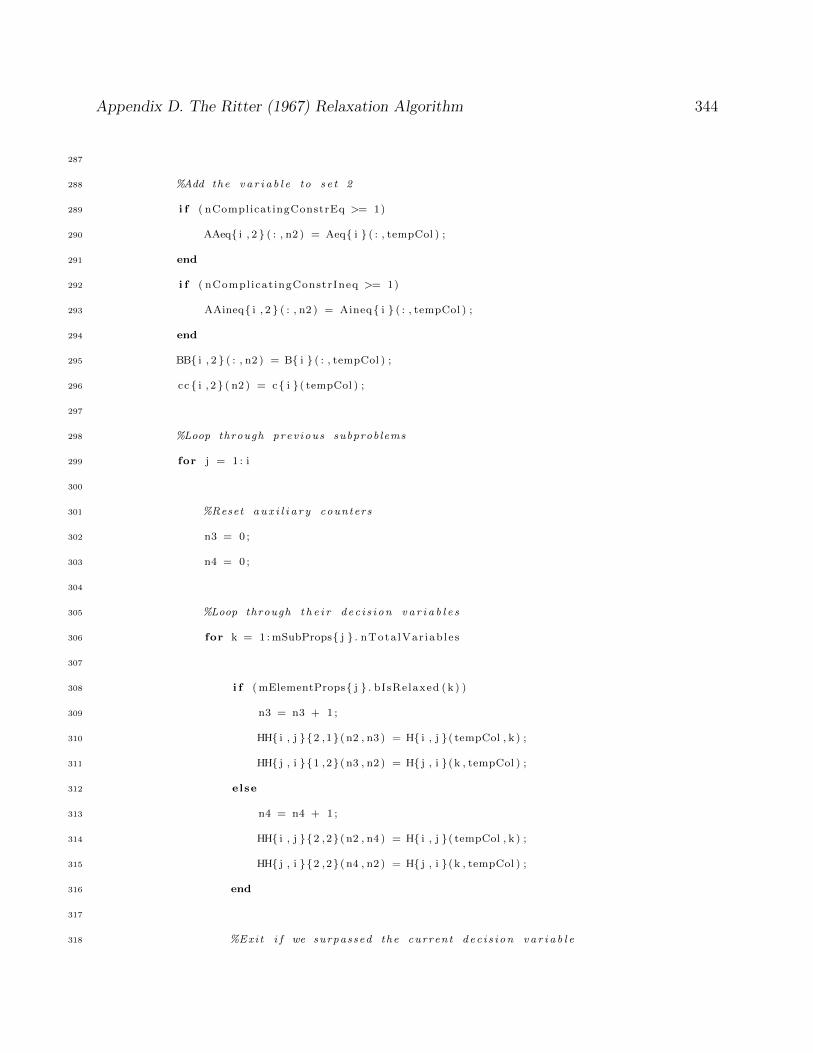
Appendix D. The Ritter (1967) Relaxation Algorithm 344
287
288 %Add the v a r i a b l e to s e t 2
289 i f ( nComplicatingConstrEq >= 1)
290 AAeq{ i , 2 } ( : , n2 ) = Aeq{ i } ( : , tempCol ) ;
291 end
292 i f ( nComplicat ingConstrIneq >= 1)
293 AAineq{ i , 2 } ( : , n2 ) = Aineq{ i } ( : , tempCol ) ;
294 end
295 BB{ i , 2 } ( : , n2 ) = B{ i } ( : , tempCol ) ;
296 cc { i , 2} ( n2 ) = c{ i }( tempCol ) ;
297
298 %Loop through prev ious subproblems
299 for j = 1 : i
300
301 %Reset a u x i l i a r y counters
302 n3 = 0 ;
303 n4 = 0 ;
304
305 %Loop through t h e i r dec i s i on v a r i a b l e s
306 for k = 1 : mSubProps{ j } . nTota lVar iab le s
307
308 i f ( mElementProps{ j } . bIsRelaxed ( k ) )
309 n3 = n3 + 1 ;
310 HH{ i , j }{2 ,1}( n2 , n3 ) = H{ i , j }( tempCol , k ) ;
311 HH{ j , i }{1 ,2}( n3 , n2 ) = H{ j , i }(k , tempCol ) ;
312 else
313 n4 = n4 + 1 ;
314 HH{ i , j }{2 ,2}( n2 , n4 ) = H{ i , j }( tempCol , k ) ;
315 HH{ j , i }{2 ,2}( n4 , n2 ) = H{ j , i }(k , tempCol ) ;
316 end
317
318 %Exi t i f we surpassed the current dec i s i on v a r i a b l e
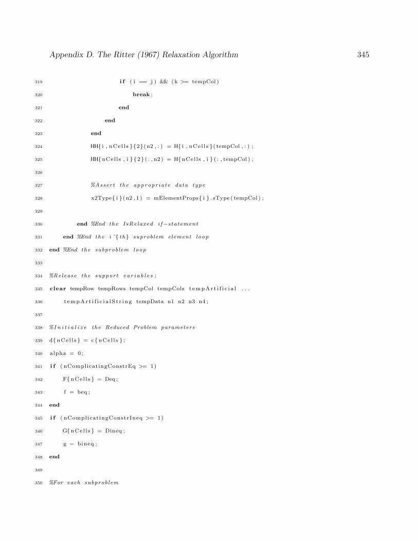
Appendix D. The Ritter (1967) Relaxation Algorithm 345
319 i f ( i == j ) && ( k >= tempCol )
320 break ;
321 end
322 end
323 end
324 HH{ i , nCe l l s }{2}(n2 , : ) = H{ i , nCe l l s }( tempCol , : ) ;
325 HH{nCel l s , i }{2} ( : , n2 ) = H{nCel l s , i } ( : , tempCol ) ;
326
327 %Assert the appropr ia te data type
328 x2Type{ i }( n2 , 1 ) = mElementProps{ i } . sType ( tempCol ) ;
329
330 end %End the IsRelaxed i f−s tatement
331 end %End the i ˆ{ th } suproblem element loop
332 end %End the subproblem loop
333
334 %Release the support v a r i a b l e s ;
335 clear tempRow tempRows tempCol tempCols t e m p A r t i f i c i a l . . .
336 t e m p A r t i f i c i a l S t r i n g tempData n1 n2 n3 n4 ;
337
338 %I n i t i a l i z e the Reduced Problem parameters
339 d{ nCe l l s } = c{ nCe l l s } ;
340 alpha = 0 ;
341 i f ( nComplicatingConstrEq >= 1)
342 F{ nCe l l s } = Deq ;
343 f = beq ;
344 end
345 i f ( nComplicat ingConstrIneq >= 1)
346 G{ nCe l l s } = Dineq ;
347 g = bineq ;
348 end
349
350 %For each subproblem
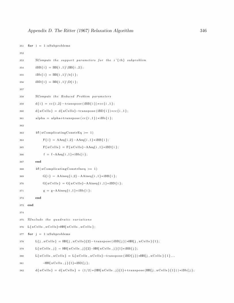
Appendix D. The Ritter (1967) Relaxation Algorithm 346
351 for i = 1 : nSubproblems
352
353 %Compute the support parameters f o r the i ˆ{ th } subproblem
354 iBB{ i } = BB{ i , 1}\BB{ i , 2 } ;
355 iBb{ i } = BB{ i , 1}\b{ i } ;
356 iBD{ i } = BB{ i , 1}\D{ i } ;
357
358 %Compute the Reduced Problem parameters
359 d{ i } = cc { i ,2}− t ranspose ( iBB{ i }) ∗ cc { i , 1 } ;
360 d{ nCe l l s } = d{ nCe l l s}−t ranspose ( iBD{ i }) ∗ cc { i , 1 } ;
361 alpha = alpha+transpose ( cc { i , 1} ) ∗ iBb{ i } ;
362
363 i f ( nComplicatingConstrEq >= 1)
364 F{ i } = AAeq{ i ,2}−AAeq{ i , 1}∗ iBB{ i } ;
365 F{ nCe l l s } = F{ nCe l l s}−AAeq{ i , 1}∗ iBD{ i } ;
366 f = f−AAeq{ i , 1}∗ iBb{ i } ;
367 end
368 i f ( nComplicat ingConstrIneq >= 1)
369 G{ i } = AAineq{ i ,2}−AAineq{ i , 1}∗ iBB{ i } ;
370 G{ nCe l l s } = G{ nCe l l s}−AAineq{ i , 1}∗ iBD{ i } ;
371 g = g−AAineq{ i , 1}∗ iBb{ i } ;
372 end
373 end
374
375 %Inc lude the quadra t i c v a r i a t i on s
376 L{nCel l s , nCe l l s}=HH{nCel l s , nCe l l s } ;
377 for j = 1 : nSubproblems
378 L{ j , nCe l l s } = HH{ j , nCe l l s }{2}− t ranspose ( iBB{ j }) ∗HH{ j , nCe l l s }{1} ;
379 L{nCel l s , j } = HH{nCel l s , j }{2}−HH{nCel l s , j }{1}∗ iBB{ j } ;
380 L{nCel l s , nCe l l s } = L{nCel l s , nCe l l s}−t ranspose ( iBD{ j }) ∗HH{ j , nCe l l s } { 1 } . . .
381 −HH{nCel l s , j }{1}∗ iBD{ j } ;
382 d{ nCe l l s } = d{ nCe l l s } + (1/2) ∗(HH{nCel l s , j }{1}+ transpose (HH{ j , nCe l l s }{1}) ) ∗ iBb{ j } ;
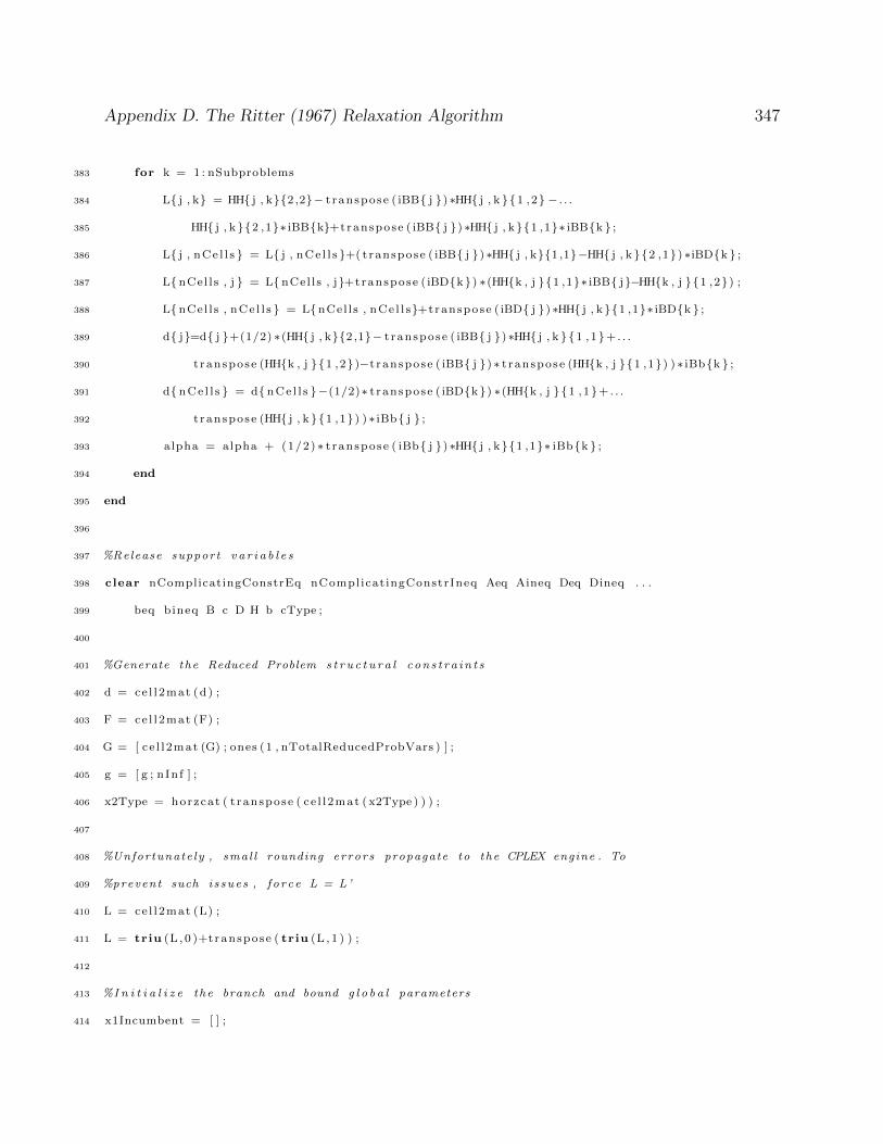
Appendix D. The Ritter (1967) Relaxation Algorithm 347
383 for k = 1 : nSubproblems
384 L{ j , k} = HH{ j , k}{2 ,2}− t ranspose ( iBB{ j }) ∗HH{ j , k }{1 ,2} − . . .
385 HH{ j , k}{2 ,1}∗ iBB{k}+transpose ( iBB{ j }) ∗HH{ j , k}{1 ,1}∗ iBB{k } ;
386 L{ j , nCe l l s } = L{ j , nCe l l s }+( transpose ( iBB{ j }) ∗HH{ j , k}{1 ,1}−HH{ j , k }{2 ,1}) ∗iBD{k } ;
387 L{nCel l s , j } = L{nCel l s , j}+transpose ( iBD{k}) ∗(HH{k , j }{1 ,1}∗ iBB{ j}−HH{k , j }{1 ,2}) ;
388 L{nCel l s , nCe l l s } = L{nCel l s , nCe l l s}+transpose ( iBD{ j }) ∗HH{ j , k}{1 ,1}∗ iBD{k } ;
389 d{ j}=d{ j }+(1/2) ∗(HH{ j , k}{2 ,1}− t ranspose ( iBB{ j }) ∗HH{ j , k }{1 , 1}+. . .
390 t ranspose (HH{k , j }{1 ,2})−t ranspose ( iBB{ j }) ∗ t ranspose (HH{k , j }{1 ,1}) ) ∗ iBb{k } ;
391 d{ nCe l l s } = d{ nCe l l s }−(1/2)∗ t ranspose ( iBD{k}) ∗(HH{k , j }{1 , 1}+. . .
392 t ranspose (HH{ j , k }{1 ,1}) ) ∗ iBb{ j } ;
393 alpha = alpha + (1/2) ∗ t ranspose ( iBb{ j }) ∗HH{ j , k}{1 ,1}∗ iBb{k } ;
394 end
395 end
396
397 %Release support v a r i a b l e s
398 clear nComplicatingConstrEq nComplicat ingConstrIneq Aeq Aineq Deq Dineq . . .
399 beq bineq B c D H b cType ;
400
401 %Generate the Reduced Problem s t r u c t u r a l c on s t r a i n t s
402 d = ce l l 2mat (d) ;
403 F = ce l l2mat (F) ;
404 G = [ ce l l 2mat (G) ; ones (1 , nTotalReducedProbVars ) ] ;
405 g = [ g ; n In f ] ;
406 x2Type = horzcat ( t ranspose ( ce l l 2mat ( x2Type ) ) ) ;
407
408 %Unfortunate ly , smal l rounding er ror s propagate to the CPLEX engine . To
409 %prevent such i s sues , f o r ce L = L’
410 L = ce l l 2mat (L) ;
411 L = triu (L , 0 )+transpose ( triu (L , 1 ) ) ;
412
413 %I n i t i a l i z e the branch and bound g l o b a l parameters
414 x1Incumbent = [ ] ;

Appendix D. The Ritter (1967) Relaxation Algorithm 348
415 x2Incumbent = [ ] ;
416 bLBViolated = f a l s e ;
417 bUBViolated = f a l s e ;
418 nOutputIterat ion = 1 ;
419 nOutputLargeIterat ion = 1 ;
420
421 %NL STRUCTURE:
422 %Added Constra in t s | Added RHS | Added Constra in t s Proper t i e s | LowerBound
423 NL = { [ ] , [ ] , mEnforcedConstraints , Inf } ;
424 nOutputNLSize = 1 ;
425
426 %Set d e f a u l t CPLEX opt ions
427 opt ions = cp lexopt imset ;
428 opt ions . D iagnos t i c s = ’ o f f ’ ;
429
430 %Output s t a t u s
431 disp ( ’ I t e r a t i o n | Nodes Le f t | Incumbent ’ ) ;
432
433 %Generate and s o l v e the Reduced Problem i t e r a t i v e l y
434 while ( ( nOutputNLSize > 0) | | ( bLBViolated ) | | ( bUBViolated ) )
435
436 %Reset g l o b a l f l a g s
437 bFathomInfeas ib le = f a l s e ;
438
439 %Retr ieve the f i r s t Reduced Problem . Here a FIFO approach i s f o l l owed .
440 %The algori thm , however , can be modi f ied to f o l l ow a d i f f e r e n t
441 %branching s t ra t e gy , i f so de s i r ed .
442 i f ( (˜ bLBViolated ) && (˜ bUBViolated ) )
443 rCons t ra in t s = NL{1 ,1} ;
444 rRHS = NL{1 ,2} ;
445 mEnforcedConstraints = NL{1 ,3} ;
446 NL( 1 , : ) = [ ] ;

Appendix D. The Ritter (1967) Relaxation Algorithm 349
447
448 %Update the i t e r a t i o n number
449 sOutput . n I t e r a t i o n s = sOutput . n I t e r a t i o n s + 1 ;
450 nOutputNLSize = nOutputNLSize − 1 ;
451
452 %Output s t a t u s
453 i f ( nOutputLargeIterat ion == 10∗ nOutputIterat ion )
454 nNLClass = whos( ’NL ’ ) ;
455 disp ( s t r c a t ( [ ’ ∗∗∗ Time Elapsed : ’ , ’ ’ , . . .
456 sprintf ( ’ %.2 f ’ ,etime ( clock , sOutput . nSolutionTime ) ) , . . .
457 ’ seconds | Tree S i z e : ’ , ’ ’ , . . .
458 sprintf ( ’ %.2 f ’ , nNLClass . bytes /(1024ˆ3) ) , ’ GB ∗∗∗ ’ ] ) ) ;
459 disp ( ’ I t e r a t i o n | Nodes Le f t | Incumbent ’ ) ;
460 nOutputLargeIterat ion = 1 ;
461 clear nNLClass ;
462 else
463 nOutputLargeIterat ion = nOutputLargeIterat ion +1;
464 end
465
466 i f ( nOutputIterat ion == nOutput I t e ra t i on In t e rva l )
467
468 %Update counter
469 nOutputIterat ion = 1 ;
470
471 %Disp lay output
472 i f ( sOutput . nObjValue == Inf )
473 disp ( s t r c a t ( [num2str( sOutput . n I t e r a t i o n s ) , ’ ’ , . . .
474 num2str( nOutputNLSize ) , ’ − ’ ] ) ) ;
475 else
476 disp ( s t r c a t ( [num2str( sOutput . n I t e r a t i o n s ) , ’ ’ , . . .
477 num2str( nOutputNLSize ) , ’ ’ ,num2str( sOutput . nObjValue ) ] ) ) ;
478 end
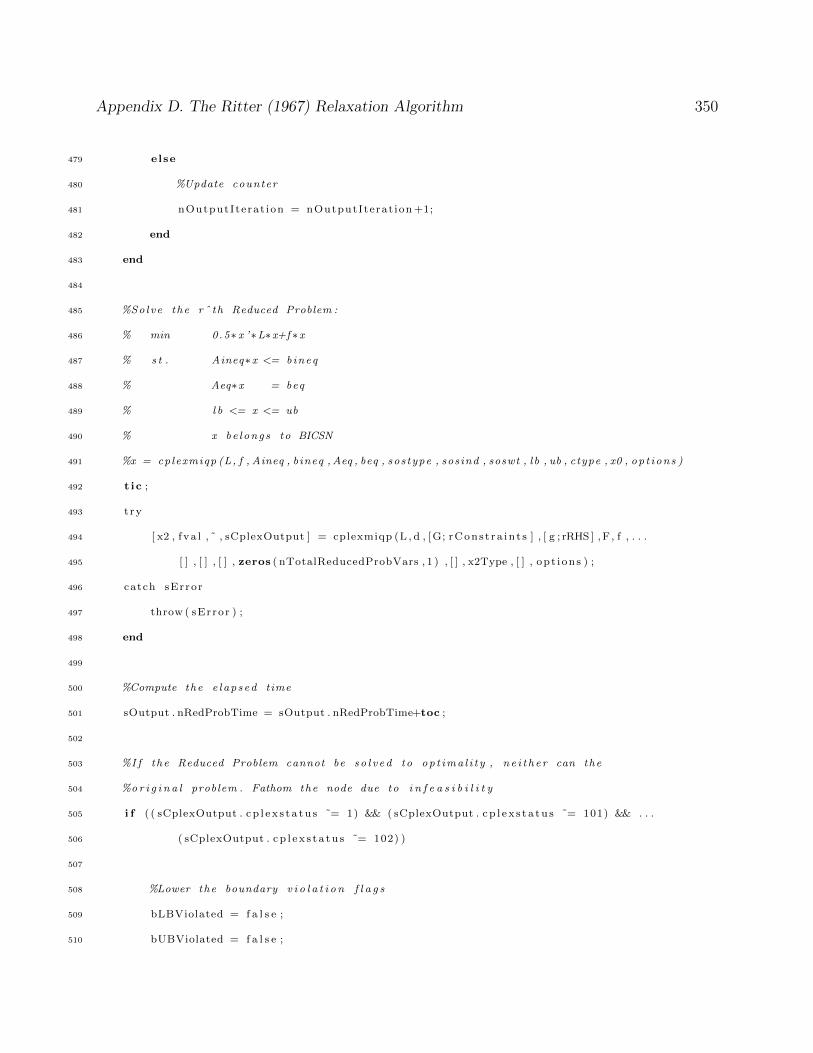
Appendix D. The Ritter (1967) Relaxation Algorithm 350
479 else
480 %Update counter
481 nOutputIterat ion = nOutputIterat ion +1;
482 end
483 end
484
485 %Solve the rˆ th Reduced Problem :
486 % min 0.5∗ x ’∗L∗x+f ∗x
487 % s t . Aineq∗x <= bineq
488 % Aeq∗x = beq
489 % l b <= x <= ub
490 % x be longs to BICSN
491 %x = cplexmiqp (L, f , Aineq , bineq ,Aeq , beq , sos type , sosind , soswt , l b , ub , ctype , x0 , op t ions )
492 t ic ;
493 t ry
494 [ x2 , f va l , ˜ , sCplexOutput ] = cplexmiqp (L , d , [G; rCons t ra in t s ] , [ g ; rRHS ] , F , f , . . .
495 [ ] , [ ] , [ ] , zeros ( nTotalReducedProbVars , 1 ) , [ ] , x2Type , [ ] , opt i ons ) ;
496 catch sError
497 throw ( sError ) ;
498 end
499
500 %Compute the e l apsed time
501 sOutput . nRedProbTime = sOutput . nRedProbTime+toc ;
502
503 %I f the Reduced Problem cannot be so l v ed to op t ima l i t y , ne i t h e r can the
504 %or i g i n a l problem . Fathom the node due to i n f e a s i b i l i t y
505 i f ( ( sCplexOutput . c p l e x s t a t u s ˜= 1) && ( sCplexOutput . c p l e x s t a t u s ˜= 101) && . . .
506 ( sCplexOutput . c p l e x s t a t u s ˜= 102) )
507
508 %Lower the boundary v i o l a t i o n f l a g s
509 bLBViolated = f a l s e ;
510 bUBViolated = f a l s e ;
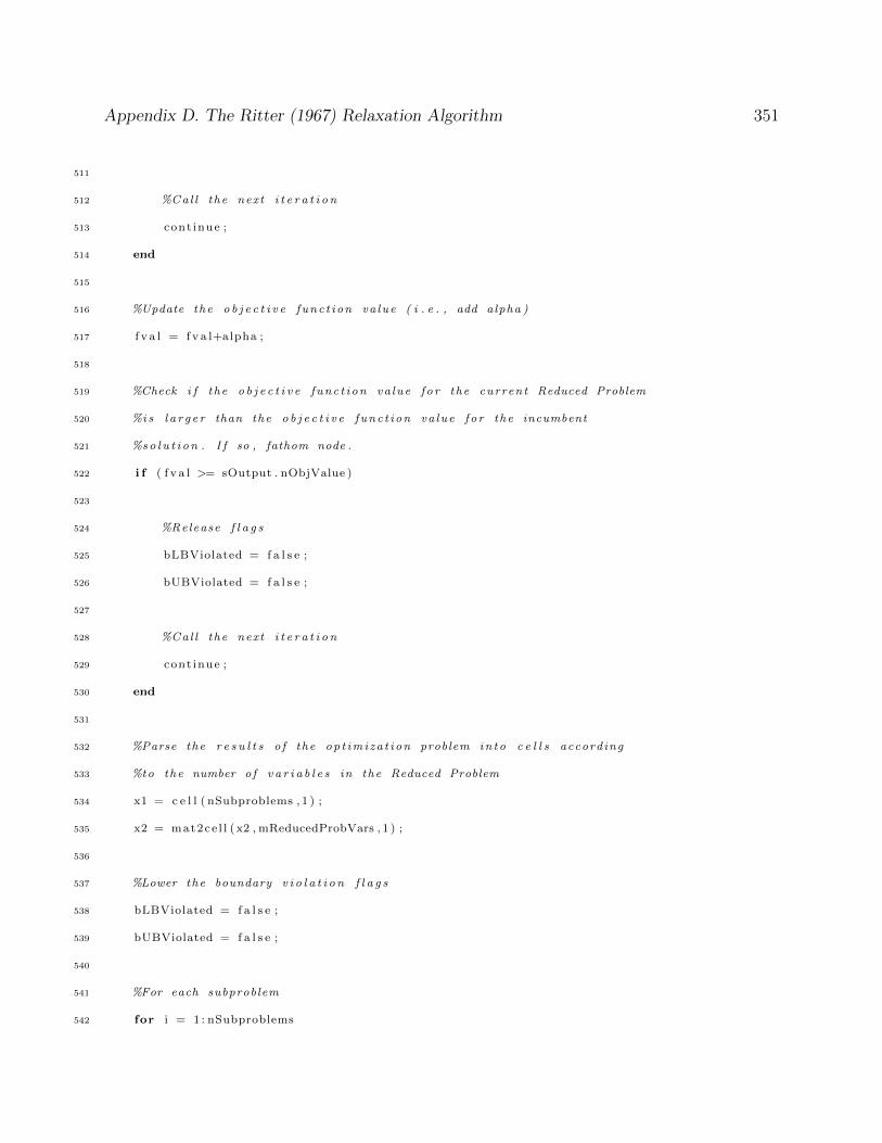
Appendix D. The Ritter (1967) Relaxation Algorithm 351
511
512 %Cal l the next i t e r a t i o n
513 cont inue ;
514 end
515
516 %Update the o b j e c t i v e func t i on va lue ( i . e . , add alpha )
517 f v a l = f v a l+alpha ;
518
519 %Check i f the o b j e c t i v e func t i on va lue f o r the current Reduced Problem
520 %i s l a r g e r than the o b j e c t i v e func t i on va lue f o r the incumbent
521 %so l u t i on . I f so , fathom node .
522 i f ( f v a l >= sOutput . nObjValue )
523
524 %Release f l a g s
525 bLBViolated = f a l s e ;
526 bUBViolated = f a l s e ;
527
528 %Cal l the next i t e r a t i o n
529 cont inue ;
530 end
531
532 %Parse the r e s u l t s o f the op t imi za t i on problem in to c e l l s according
533 %to the number o f v a r i a b l e s in the Reduced Problem
534 x1 = c e l l ( nSubproblems , 1 ) ;
535 x2 = mat2ce l l ( x2 , mReducedProbVars , 1 ) ;
536
537 %Lower the boundary v i o l a t i o n f l a g s
538 bLBViolated = f a l s e ;
539 bUBViolated = f a l s e ;
540
541 %For each subproblem
542 for i = 1 : nSubproblems
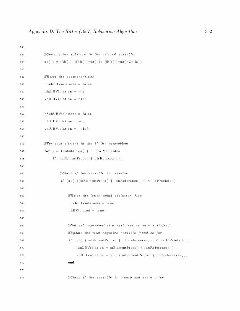
Appendix D. The Ritter (1967) Relaxation Algorithm 352
543
544 %Compute the s o l u t i on to the r e l a xed v a r i a b l e s
545 x1{ i } = iBb{ i }−(iBB{ i }∗x2{ i })−(iBD{ i }∗x2{ nCe l l s }) ;
546
547 %Reset the counters / f l a g s
548 bSubLBViolations = f a l s e ;
549 idxLBViolat ion = −1;
550 valLBVio lat ion = nIn f ;
551
552 bSubUBViolations = f a l s e ;
553 idxUBViolation = −1;
554 valUBViolat ion = −nIn f ;
555
556 %For each element in the i ˆ{ th } subproblem
557 for j = 1 : mSubProps{ i } . nTota lVar iab le s
558 i f ( mElementProps{ i } . bIsRelaxed ( j ) )
559
560 %Check i f the v a r i a b l e i s nega t i v e
561 i f ( x1{ i }( mElementProps{ i } . i dxRe fe rence ( j ) ) < −nPrec i s i on )
562
563 %Raise the lower bound v i o l a t i o n f l a g
564 bSubLBViolations = true ;
565 bLBViolated = true ;
566
567 %Not a l l non−n e g a t i v i t y r e s t r i c t i o n s were s a t i s f i e d
568 %Update the most nega t i v e v a r i a b l e found so fa r .
569 i f ( x1{ i }( mElementProps{ i } . i dxRe fe rence ( j ) ) < valLBVio lat ion )
570 idxLBViolat ion = mElementProps{ i } . i dxRe fe rence ( j ) ;
571 valLBViolat ion = x1{ i }( mElementProps{ i } . i dxRe fe rence ( j ) ) ;
572 end
573
574 %Check i f the v a r i a b l e i s b inary and has a va lue
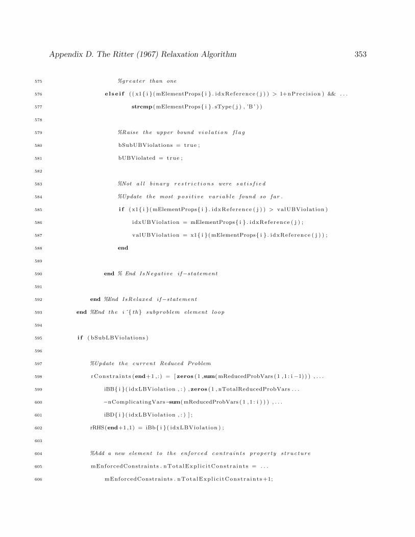
Appendix D. The Ritter (1967) Relaxation Algorithm 353
575 %grea t e r than one
576 e l s e i f ( ( x1{ i }( mElementProps{ i } . i dxRe fe rence ( j ) ) > 1+nPrec i s i on ) && . . .
577 strcmp ( mElementProps{ i } . sType ( j ) , ’B ’ ) )
578
579 %Raise the upper bound v i o l a t i o n f l a g
580 bSubUBViolations = true ;
581 bUBViolated = true ;
582
583 %Not a l l b inary r e s t r i c t i o n s were s a t i s f i e d
584 %Update the most p o s i t i v e v a r i a b l e found so fa r .
585 i f ( x1{ i }( mElementProps{ i } . i dxRe fe rence ( j ) ) > valUBViolat ion )
586 idxUBViolation = mElementProps{ i } . i dxRe fe rence ( j ) ;
587 valUBViolat ion = x1{ i }( mElementProps{ i } . i dxRe fe rence ( j ) ) ;
588 end
589
590 end % End IsNega t i ve i f−s tatement
591
592 end %End IsRelaxed i f−s tatement
593 end %End the i ˆ{ th } subproblem element loop
594
595 i f ( bSubLBViolations )
596
597 %Update the current Reduced Problem
598 rCons t ra in t s (end+1 , :) = [ zeros (1 ,sum( mReducedProbVars ( 1 , 1 : i −1) ) ) , . . .
599 iBB{ i }( idxLBViolat ion , : ) , zeros (1 , nTotalReducedProbVars . . .
600 −nComplicatingVars−sum( mReducedProbVars ( 1 , 1 : i ) ) ) , . . .
601 iBD{ i }( idxLBViolat ion , : ) ] ;
602 rRHS(end+1 ,1) = iBb{ i }( idxLBViolat ion ) ;
603
604 %Add a new element to the enforced con t ra in t s proper ty s t r u c t u r e
605 mEnforcedConstraints . nTota lExp l i c i tCons t r a in t s = . . .
606 mEnforcedConstraints . nTota lExp l i c i tCons t r a in t s +1;

Appendix D. The Ritter (1967) Relaxation Algorithm 354
607 mEnforcedConstraints . nSubproblem (end+1 ,1) = i ;
608 mEnforcedConstraints . nElement (end+1 ,1) = idxLBViolat ion ;
609 mEnforcedConstraints . nRowReference (end+1 ,1) = . . .
610 mEnforcedConstraints . nTota lExp l i c i tCons t r a in t s ;
611 mEnforcedConstraints . bUpperBoundRestriction (end+1 ,1) = f a l s e ;
612
613 e l s e i f ( bSubUBViolations )
614
615 %Update the current Reduced Problem
616 rCons t ra in t s (end+1 , :) = [ zeros (1 ,sum( mReducedProbVars ( 1 , 1 : i −1) ) ) , . . .
617 −iBB{ i }( idxUBViolation , : ) , zeros (1 , nTotalReducedProbVars . . .
618 −nComplicatingVars−sum( mReducedProbVars ( 1 , 1 : i ) ) ) , . . .
619 −iBD{ i }( idxUBViolation , : ) ] ;
620 rRHS(end+1 ,1) = 1−iBb{ i }( idxUBViolation ) ;
621
622 %Add a new element to the enforced con t ra in t s proper ty s t r u c t u r e
623 mEnforcedConstraints . nTota lExp l i c i tCons t r a in t s = . . .
624 mEnforcedConstraints . nTota lExp l i c i tCons t r a in t s +1;
625 mEnforcedConstraints . nSubproblem (end+1 ,1) = i ;
626 mEnforcedConstraints . nElement (end+1 ,1) = idxUBViolation ;
627 mEnforcedConstraints . nRowReference (end+1 ,1) = . . .
628 mEnforcedConstraints . nTota lExp l i c i tCons t r a in t s ;
629 mEnforcedConstraints . bUpperBoundRestriction (end+1 ,1) = true ;
630
631 end %End HasNegatives i f−s tatement
632 end %End the subproblem loop
633
634 %Cal l the next i t e r a t i on , i f needed
635 i f ( bLBViolated )
636 cont inue ;
637 end
638
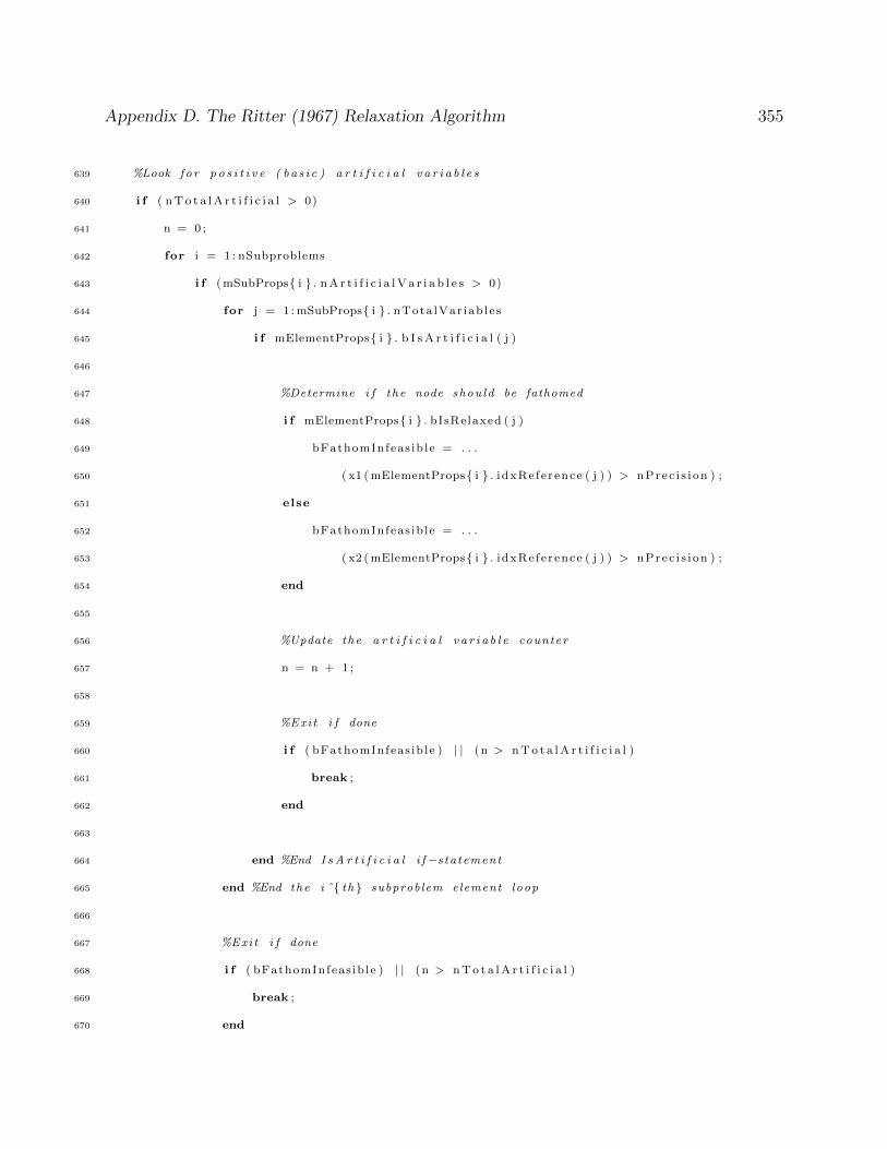
Appendix D. The Ritter (1967) Relaxation Algorithm 355
639 %Look fo r p o s i t i v e ( ba s i c ) a r t i f i c i a l v a r i a b l e s
640 i f ( n T o t a l A r t i f i c i a l > 0)
641 n = 0 ;
642 for i = 1 : nSubproblems
643 i f ( mSubProps{ i } . n A r t i f i c i a l V a r i a b l e s > 0)
644 for j = 1 : mSubProps{ i } . nTota lVar iab le s
645 i f mElementProps{ i } . b I s A r t i f i c i a l ( j )
646
647 %Determine i f the node shou ld be fathomed
648 i f mElementProps{ i } . bIsRelaxed ( j )
649 bFathomInfeas ib le = . . .
650 ( x1 ( mElementProps{ i } . i dxRe fe rence ( j ) ) > nPrec i s i on ) ;
651 else
652 bFathomInfeas ib le = . . .
653 ( x2 ( mElementProps{ i } . i dxRe fe rence ( j ) ) > nPrec i s i on ) ;
654 end
655
656 %Update the a r t i f i c i a l v a r i a b l e counter
657 n = n + 1 ;
658
659 %Exi t i f done
660 i f ( bFathomInfeas ib le ) | | (n > n T o t a l A r t i f i c i a l )
661 break ;
662 end
663
664 end %End I s A r t i f i c i a l i f−s tatement
665 end %End the i ˆ{ th } subproblem element loop
666
667 %Exi t i f done
668 i f ( bFathomInfeas ib le ) | | (n > n T o t a l A r t i f i c i a l )
669 break ;
670 end
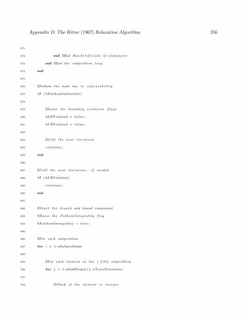
Appendix D. The Ritter (1967) Relaxation Algorithm 356
671
672 end %End Ha sAr t i f i c i a l s i f−s tatement
673 end %End the subproblem loop
674 end
675
676 %Fathom the node due to i n f e a s i b i l i t y
677 i f ( bFathomInfeas ib le )
678
679 %Lower the boundary v i o l a t i o n f l a g s
680 bLBViolated = f a l s e ;
681 bUBViolated = f a l s e ;
682
683 %Cal l the next i t e r a t i o n
684 cont inue ;
685 end
686
687 %Cal l the next i t e r a t i on , i f needed
688 i f ( bUBViolated )
689 cont inue ;
690 end
691
692 %Star t the branch and bound component
693 %Raise the FathomIntegra l i t y f l a g
694 bFathomIntegra l i ty = true ;
695
696 %For each subproblem
697 for i = 1 : nSubproblems
698
699 %For each element in the i ˆ{ th } subproblem
700 for j = 1 : mSubProps{ i } . nTota lVar iab le s
701
702 %Check i f the element i s i n t e g e r

Appendix D. The Ritter (1967) Relaxation Algorithm 357
703 i f mElementProps{ i } . bIsRelaxed ( j )
704 i f (strcmp ( mElementProps{ i } . sType ( j ) , ’B ’ ) | | . . .
705 strcmp ( mElementProps{ i } . sType ( j ) , ’ I ’ ) )
706 n = abs ( x1{ i }( mElementProps{ i } . i dxRe fe rence ( j ) ) ) ;
707 i f ( ( ( ce i l (n)−n) > nPrec i s i on ) && . . .
708 ( ( n−f loor (n) ) > nPrec i s i on ) )
709 bFathomIntegra l i ty = f a l s e ;
710 break ;
711 end %End ˜ I s I n t e g e r i f−s tatement
712 end %End I s In t e g e rRe s t r i c e d i f−s tatement
713 end %End IsRelaxed i f−s tatement
714
715 end %End the i ˆ{ th } subproblem element loop
716 i f (˜ bFathomIntegra l i ty )
717 break ;
718 end
719 end %End the subproblem loop
720
721 i f ( bFathomIntegra l i ty )
722 i f ( f v a l < sOutput . nObjValue )
723
724 %Save the new in t e g e r o b j e c t i v e func t i on va lue
725 sOutput . nObjValue = f v a l ;
726 x1Incumbent = x1 ;
727 x2Incumbent = x2 ;
728
729 %Loop through the Reduced Problem l i s t and fathom nodes with
730 %lower bound grea t e r than or equa l to f v a l
731 i f ( nOutputNLSize >= 1)
732 i f (NL{1 ,4} >= sOutput . nObjValue )
733 %Since the NL i s ordered , i f the o b j e c t i v e func t i on
734 %value o f i t s f i r s t e lement i s l a r g e r than or equa l to

Appendix D. The Ritter (1967) Relaxation Algorithm 358
735 %the o b j e c t i v e func t i on va lue o f the incumbent so lu t i on ,
736 %then fathom the en t i r e l i s t .
737 NL = [ ] ;
738 nOutputNLSize = 0 ;
739
740 e l s e i f (NL{nOutputNLSize , 4} >= sOutput . nObjValue )
741 %I f the o b j e c t i v e func t i on va lue o f the incumbent s o l u t i on
742 %l i e s between the o b j e c t i v e func t i on va lue o f NL’ s
743 %f i r s t and l a s t elements , then perform a dichotomous
744 %search fo r the s t a r t i n g element to be fathomed
745 nPosStart = 1 ;
746 nPosEnd = nOutputNLSize ;
747 nPos = f loor ((1+nOutputNLSize ) /2) ;
748 while ( ( nPosEnd−nPosStart ) > 1)
749 i f (NL{nPos ,4} > sOutput . nObjValue )
750 nPosEnd = nPos ;
751 nPos = f loor ( ( nPosStart+nPosEnd ) /2) ;
752 e l s e i f (NL{nPos ,4} < sOutput . nObjValue )
753 nPosStart = nPos ;
754 nPos = ce i l ( ( nPosStart+nPosEnd ) /2) ;
755 else
756 break ;
757 end
758 end
759 nPos = nPosEnd ;
760 NL( nPos : nOutputNLSize , : ) = [ ] ;
761 nOutputNLSize = nPos−1;
762 end
763 end
764 end %End HasBetterObjFnValue i f−s tatement
765
766 %Cal l the next i t e r a t i o n
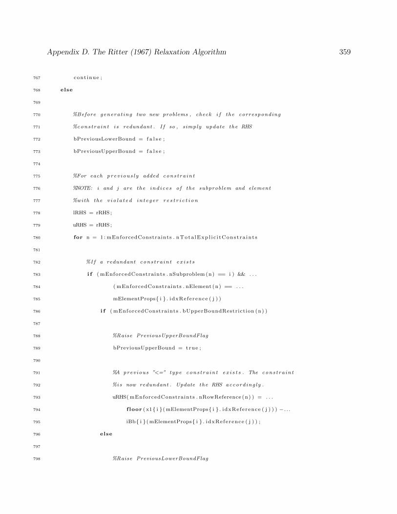
Appendix D. The Ritter (1967) Relaxation Algorithm 359
767 cont inue ;
768 else
769
770 %Before genera t ing two new problems , check i f the corresponding
771 %cons t r a in t i s redundant . I f so , s imply update the RHS
772 bPreviousLowerBound = f a l s e ;
773 bPreviousUpperBound = f a l s e ;
774
775 %For each p r e v i ou s l y added cons t r a in t
776 %NOTE: i and j are the i nd i c e s o f the subproblem and element
777 %with the v i o l a t e d i n t e g e r r e s t r i c t i o n
778 lRHS = rRHS ;
779 uRHS = rRHS ;
780 for n = 1 : mEnforcedConstraints . nTota lExp l i c i tCons t r a in t s
781
782 %I f a redundant cons t r a in t e x i s t s
783 i f ( mEnforcedConstraints . nSubproblem (n) == i ) && . . .
784 ( mEnforcedConstraints . nElement (n) == . . .
785 mElementProps{ i } . i dxRe fe rence ( j ) )
786 i f ( mEnforcedConstraints . bUpperBoundRestriction (n) )
787
788 %Raise PreviousUpperBoundFlag
789 bPreviousUpperBound = true ;
790
791 %A prev ious ”<=” type cons t r a in t e x i s t s . The cons t r a in t
792 %i s now redundant . Update the RHS accord ing l y .
793 uRHS( mEnforcedConstraints . nRowReference (n) ) = . . .
794 f loor ( x1{ i }( mElementProps{ i } . i dxRe fe rence ( j ) ) ) − . . .
795 iBb{ i }( mElementProps{ i } . i dxRe fe rence ( j ) ) ;
796 else
797
798 %Raise PreviousLowerBoundFlag

Appendix D. The Ritter (1967) Relaxation Algorithm 360
799 bPreviousLowerBound = true ;
800
801 %A prev ious ”>=” type cons t r a in t e x i s t s . The cons t r a in t
802 %i s now redundant . Update the RHS accord ing l y .
803 lRHS( mEnforcedConstraints . nRowReference (n) ) = . . .
804 −ce i l ( x1{ i }( mElementProps{ i } . i dxRe fe rence ( j ) ) )+ . . .
805 iBb{ i }( mElementProps{ i } . i dxRe fe rence ( j ) ) ;
806 end
807
808
809 %Exi t i f a l ready found a l l redundant con s t r a i n t s
810 i f ( bPreviousLowerBound ) && ( bPreviousUpperBound )
811 break ;
812 end
813
814 end %End IsRedundant i f−s tatement
815 end %End the p r e v i ou s l y added con s t r a i n t s loop
816
817 %Search the node l i s t f o r the b e s t node placement
818 i f ( nOutputNLSize == 0)
819 %I f NL i s empty , append the node
820 nPos = 1 ;
821 e l s e i f (NL{nOutputNLSize , 4} <= f v a l )
822 %I f NL i s nonempty and the bound on i t s l a s t e lement i s sma l l e r
823 %than the current bound , add the node to the back o f the l i s t
824 nPos = nOutputNLSize+1;
825 e l s e i f (NL{1 ,4} >= f v a l )
826 %I f NL i s nonempty and the bound on i t s f i r s t e lement i s l a r g e r
827 %than the current bound , add the node to the f r on t o f the l i s t
828 nPos = 1 ;
829 else
830 %I f NL i s nonempty and the current bound l i e s between the
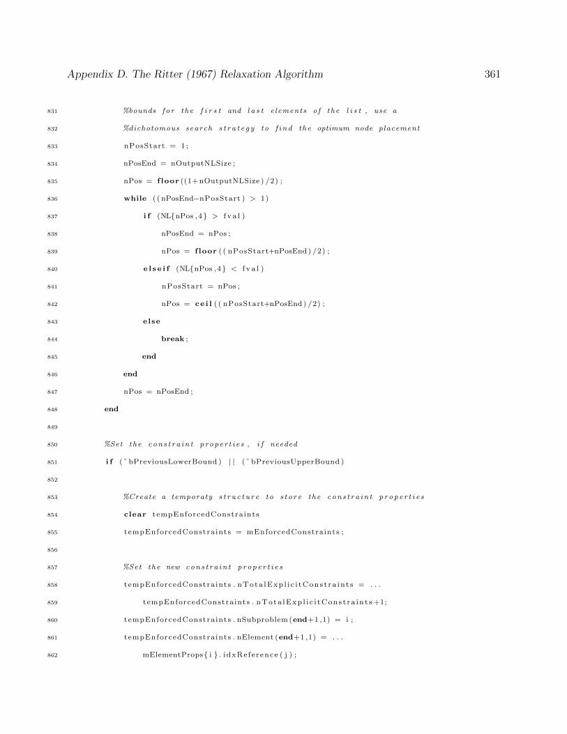
Appendix D. The Ritter (1967) Relaxation Algorithm 361
831 %bounds f o r the f i r s t and l a s t e lements o f the l i s t , use a
832 %dichotomous search s t r a t e g y to f i nd the optimum node placement
833 nPosStart = 1 ;
834 nPosEnd = nOutputNLSize ;
835 nPos = f loor ((1+nOutputNLSize ) /2) ;
836 while ( ( nPosEnd−nPosStart ) > 1)
837 i f (NL{nPos ,4} > f v a l )
838 nPosEnd = nPos ;
839 nPos = f loor ( ( nPosStart+nPosEnd ) /2) ;
840 e l s e i f (NL{nPos ,4} < f v a l )
841 nPosStart = nPos ;
842 nPos = ce i l ( ( nPosStart+nPosEnd ) /2) ;
843 else
844 break ;
845 end
846 end
847 nPos = nPosEnd ;
848 end
849
850 %Set the cons t r a in t p roper t i e s , i f needed
851 i f (˜ bPreviousLowerBound ) | | (˜ bPreviousUpperBound )
852
853 %Create a temporaty s t r u c t u r e to s t o r e the cons t r a in t p r op e r t i e s
854 clear tempEnforcedConstraints
855 tempEnforcedConstraints = mEnforcedConstraints ;
856
857 %Set the new cons t r a in t p r op e r t i e s
858 tempEnforcedConstraints . nTota lExp l i c i tCons t r a in t s = . . .
859 tempEnforcedConstraints . nTota lExp l i c i tCons t r a in t s +1;
860 tempEnforcedConstraints . nSubproblem (end+1 ,1) = i ;
861 tempEnforcedConstraints . nElement (end+1 ,1) = . . .
862 mElementProps{ i } . i dxRe fe rence ( j ) ;
Appendix D. The Ritter (1967) Relaxation Algorithm 362
863 tempEnforcedConstraints . nRowReference (end+1 ,1) = . . .
864 tempEnforcedConstraints . nTota lExp l i c i tCons t r a in t s ;
865 end
866
867 %Add the 2 new Reduced Problems to the NodeList s e t
868 NL = [NL( 1 : nPos−1 , : ) ; { [ ] , [ ] , [ ] , f v a l } ; { [ ] , [ ] , [ ] , f v a l } ;NL( nPos : nOutputNLSize , : ) ] ;
869 nOutputNLSize = nOutputNLSize+2;
870
871 i f ( bPreviousLowerBound )
872 %Add the e x i s t i n g cons t r a in t s e t and the update RHS vec tor
873 NL{nPos ,1} = rCons t ra in t s ;
874 NL{nPos ,2} = lRHS ;
875 NL{nPos ,3} = mEnforcedConstraints ;
876 else
877 %Append a new cons t r a in t in to the e x i s t i n g cons t r a in t s e t
878 NL{nPos ,1} = [ rCons t ra in t s ; zeros (1 ,sum( mReducedProbVars ( 1 , 1 : i −1) ) ) , . . .
879 iBB{ i }( mElementProps{ i } . i dxRe fe rence ( j ) , : ) , . . .
880 zeros (1 , nTotalReducedProbVars−nComplicatingVars . . .
881 −sum( mReducedProbVars ( 1 , 1 : i ) ) ) , . . .
882 iBD{ i }( mElementProps{ i } . i dxRe fe rence ( j ) , : ) ] ;
883
884 NL{nPos ,2} = [ rRHS;− ce i l ( x1{ i }( mElementProps{ i } . i dxRe fe rence ( j ) ) )+ . . .
885 iBb{ i }( mElementProps{ i } . i dxRe fe rence ( j ) ) ] ;
886
887 tempEnforcedConstraints . bUpperBoundRestriction (end+1 ,1) = f a l s e ;
888 NL{nPos ,3} = tempEnforcedConstra ints ;
889 end
890
891 i f ( bPreviousUpperBound )
892 %Add the e x i s t i n g cons t r a in t s e t and the update RHS vec tor
893 NL{nPos+1 ,1} = rCons t ra in t s ;
894 NL{nPos+1 ,2} = uRHS;

Appendix D. The Ritter (1967) Relaxation Algorithm 363
895 NL{nPos+1 ,3} = mEnforcedConstraints ;
896 else
897 %Append a new cons t r a in t in to the e x i s t i n g cons t r a in t s e t
898 NL{nPos+1 ,1} = [ rCons t ra in t s ; . . .
899 zeros (1 ,sum( mReducedProbVars ( 1 , 1 : i −1) ) ) , . . .
900 −iBB{ i }( mElementProps{ i } . i dxRe fe rence ( j ) , : ) , . . .
901 zeros (1 , nTotalReducedProbVars−nComplicatingVars . . .
902 −sum( mReducedProbVars ( 1 , 1 : i ) ) ) , . . .
903 −iBD{ i }( mElementProps{ i } . i dxRe fe rence ( j ) , : ) ] ;
904
905 NL{nPos+1 ,2} = [ rRHS ; f loor ( x1{ i }( mElementProps{ i } . i dxRe fe rence ( j ) ) )− . . .
906 iBb{ i }( mElementProps{ i } . i dxRe fe rence ( j ) ) ] ;
907
908 tempEnforcedConstraints . bUpperBoundRestriction (end+1 ,1) = true ;
909 NL{nPos+1 ,3} = tempEnforcedConstra ints ;
910 end
911 end %End IsFa thomIn teg ra l i t y i f−s tatement
912 end %End main wh i l e loop
913
914 %Release the support v a r i a b l e s
915 clear AAeq AAineq BB HH cc iBB iBb iBD L d F f G g alpha x1 x2 NL f v a l k . . .
916 idxLBViolat ion valLBVio lat ion idxUBViolation valUBViolat ion . . .
917 bSubLBViolations bLBViolated bSubUBViolations bUBViolated x2Type . . .
918 bFathomInfeas ib le bFathomIntegra l i ty rCons t ra in t s rRHS n T o t a l A r t i f i c i a l . . .
919 mEnforcedConstraints opt ions bPreviousLowerBound bPreviousUpperBound . . .
920 lRHS uRHS nOutputNLSize tempEnforcedConstra ints nPos nPosStart nPosEnd . . .
921 nComplicatingVars nTotalReducedProbVars mReducedProbVars nOutputIterat ion . . .
922 sCplexOutput nOutput I t e ra t i on In t e rva l ;
923
924 %Output Resu l t s
925 switch true
926 case sOutput . nObjValue == Inf
Appendix D. The Ritter (1967) Relaxation Algorithm 364
927 sOutput . sResu l t = ’ i n f e a s i b l e ’ ;
928 sOutput . s D e s c r i p t i o n = ’The o r i g i n a l problem i s i n f e a s i b l e ’ ;
929
930 case (sum( ce l l 2mat ( x2Incumbent ) ) > nIn f − nPrec i s i on )
931 sOutput . sResu l t = ’ unbounded ’ ;
932 sOutput . s D e s c r i p t i o n = ’The o r i g i n a l problem i s unbounded ’ ;
933
934 otherw i se
935 sOutput . sResu l t = ’ optimal ’ ;
936 sOutput . s D e s c r i p t i o n = ’ Program Fin i shed . Optimal s o l u t i o n found ’ ;
937
938 %In s t an t i a t e the s o l u t i on s e t
939 sOutput . x = c e l l ( nCel l s , 1 ) ;
940
941 %For each subproblem
942 for i = 1 : nSubproblems
943
944 %I n i t i a l i z e s o l u t i on matrix
945 sOutput . x{ i } = zeros ( mSubProps{ i } . nRealVar iables , 1 ) ;
946
947 %For each element in the i ˆ{ th } subproblem
948 n = 0 ;
949 for j = 1 : mSubProps{ i } . nTota lVar iab le s
950 i f (˜ mElementProps{ i } . b I s A r t i f i c i a l ( j ) )
951
952 %Update counter
953 n = n + 1 ;
954
955 %Merge the r e l a xed and non−r e l a xed s e t s
956 i f ( mElementProps{ i } . bIsRelaxed ( j ) )
957 sOutput . x{ i }(n) = x1Incumbent{ i }( mElementProps{ i } . i dxRe fe rence ( j ) ) ;
958 else
Appendix D. The Ritter (1967) Relaxation Algorithm 365
959 sOutput . x{ i }(n) = x2Incumbent{ i }( mElementProps{ i } . i dxRe fe rence ( j ) ) ;
960 end
961
962 end %End I s A r t i f i c i a l i f−s tatement
963 end %End the i ˆ{ th } subproblem element loop
964 end %End the subproblem loop
965
966 %Inc lude f i n a l va lue o f comp l i ca t ing v a r i a b l e s
967 sOutput . x{nCel l s , 1} = x2Incumbent{nCel l s , 1 } ;
968
969 end %End swi tch
970
971 %Compute the e l apsed time
972 sOutput . nSolutionTime = etime ( clock , sOutput . nSolutionTime ) ;
973 disp ( sOutput )
974
975 %Release the remaining support v a r i a b l e s
976 clear i j n mSubProps mElementProps nIn f nPrec i s i on x1Incumbent x2Incumbent . . .
977 nCe l l s nSubproblems ;
978 end %End Function
Appendix E
Iterative Algorithm for the D-VRP
Variation of the BEP - Source Code:
IBM ILOG CPLEX Optimization
Studio version 12.5
366

Appendix E. Iterative Algorithm for the D-VRP Variation of the BEP 367
E.1 Two-Stage Stochastic Formulation
E.1.1 Model File (BaseModel.mod)
1 // MODEL FILE
2
3 // Import Network Parameters
4 { s t r i n g } S = . . . ; // Set o f Depots
5 { s t r i n g } P = . . . ; // Set o f Pick−up Locat ions
6 { s t r i n g } N =(S union P) ; // Set o f Nodes
7 { s t r i n g } C = . . . ; // Set o f Scenarios
8
9 tup l e Arcs { s t r i n g o r i g ; s t r i n g dest ; } ; // Set o f Arcs
10 {Arcs} A with o r i g in N, des t in N = . . . ;
11
12 int V = . . . ; // F l e e t S i ze Ava i l a b l e
13 range VRange = 1 . .V;
14
15 f loat time [A] = . . . ; // Arc Traversa l Times
16 f loat Dmnd[P ] [ C] = . . . ; // Pos s i b l e Demand Rea l i z a t i on s
17
18 // Determine the Upper Bound on T
19 int T = . . . ;
20 range TRange = 1 . .T;
21
22 int ConstrainedT = . . . ;
23
24 // Set o f Previous Arc Traversa l s
25 tup l e rSta r {Arcs arc ; int v e h i c l e ; int t r a v e r s a l ; } ;
26 { rS ta r } R Star with arc in A, v e h i c l e in VRange , t r a v e r s a l in TRange = . . . ;
27
28 // Set o f Previous V i s i t s to Pick−up Locat ions
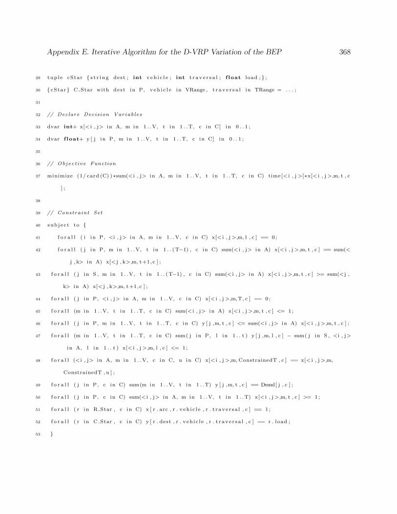
Appendix E. Iterative Algorithm for the D-VRP Variation of the BEP 368
29 tup l e cStar { s t r i n g dest ; int v e h i c l e ; int t r a v e r s a l ; f loat load ; } ;
30 { cStar } C Star with dest in P, v e h i c l e in VRange , t r a v e r s a l in TRange = . . . ;
31
32 // Declare Decis ion Var iab l e s
33 dvar int+ x[< i , j> in A, m in 1 . .V, t in 1 . . T, c in C] in 0 . . 1 ;
34 dvar f loat+ y [ j in P, m in 1 . .V, t in 1 . . T, c in C] in 0 . . 1 ;
35
36 // Ob j ec t i v e Function
37 minimize (1/ card (C) ) ∗sum(< i , j> in A, m in 1 . .V, t in 1 . . T, c in C) time [< i , j >]∗x[< i , j>,m, t , c
] ;
38
39 // Constra int Set
40 s ub j e c t to {
41 f o r a l l ( i in P, <i , j> in A, m in 1 . .V, c in C) x[< i , j>,m, 1 , c ] == 0 ;
42 f o r a l l ( j in P, m in 1 . .V, t in 1 . . ( T−1) , c in C) sum(< i , j> in A) x[< i , j>,m, t , c ] == sum(<
j , k> in A) x[< j , k>,m, t +1,c ] ;
43 f o r a l l ( j in S , m in 1 . .V, t in 1 . . ( T−1) , c in C) sum(< i , j> in A) x[< i , j>,m, t , c ] >= sum(< j ,
k> in A) x[< j , k>,m, t +1,c ] ;
44 f o r a l l ( j in P, <i , j> in A, m in 1 . .V, c in C) x[< i , j>,m,T, c ] == 0 ;
45 f o r a l l (m in 1 . .V, t in 1 . . T, c in C) sum(< i , j> in A) x[< i , j>,m, t , c ] <= 1 ;
46 f o r a l l ( j in P, m in 1 . .V, t in 1 . . T, c in C) y [ j ,m, t , c ] <= sum(< i , j> in A) x[< i , j>,m, t , c ] ;
47 f o r a l l (m in 1 . .V, t in 1 . . T, c in C) sum( j in P, l in 1 . . t ) y [ j ,m, l , c ] − sum( j in S , <i , j>
in A, l in 1 . . t ) x[< i , j>,m, l , c ] <= 1 ;
48 f o r a l l (< i , j> in A, m in 1 . .V, c in C, u in C) x[< i , j>,m, ConstrainedT , c ] == x[< i , j>,m,
ConstrainedT , u ] ;
49 f o r a l l ( j in P, c in C) sum(m in 1 . .V, t in 1 . .T) y [ j ,m, t , c ] == Dmnd[ j , c ] ;
50 f o r a l l ( j in P, c in C) sum(< i , j> in A, m in 1 . .V, t in 1 . .T) x[< i , j>,m, t , c ] >= 1 ;
51 f o r a l l ( r in R Star , c in C) x [ r . arc , r . v eh i c l e , r . t r a v e r s a l , c ] == 1 ;
52 f o r a l l ( r in C Star , c in C) y [ r . dest , r . v eh i c l e , r . t r a v e r s a l , c ] == r . load ;
53 }
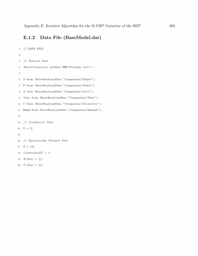
Appendix E. Iterative Algorithm for the D-VRP Variation of the BEP 369
E.1.2 Data File (BaseModel.dat)
1 // DATA FILE
2
3 // Network Data
4 SheetConnection myData( ”BEP−Probing . x l sx ” ) ;
5
6 S from SheetRead (myData , ”Comparison ! Depot” ) ;
7 P from SheetRead (myData , ”Comparison ! Nodes” ) ;
8 A from SheetRead (myData , ”Comparison ! Arcs” ) ;
9 time from SheetRead (myData , ”Comparison ! Time” ) ;
10 C from SheetRead (myData , ”Comparison ! Scenar i o s ” ) ;
11 Dmnd from SheetRead (myData , ”Comparison ! Demand” ) ;
12
13 // Ana l y t i c a l Data
14 V = 2 ;
15
16 // Dynamically Changed Data
17 T = 10 ;
18 ConstrainedT = 1 ;
19 R Star = {} ;
20 C Star = {} ;
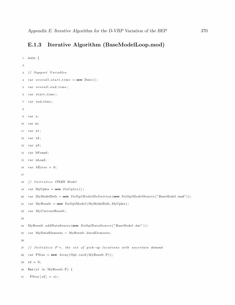
Appendix E. Iterative Algorithm for the D-VRP Variation of the BEP 370
E.1.3 Iterative Algorithm (BaseModelLoop.mod)
1 main {
2
3 // Support Var iab l e s
4 var o v e r a l l s t a r t t i m e = new Date ( ) ;
5 var o v e r a l l e n d t i m e ;
6 var s t a r t t i m e ;
7 var end time ;
8
9 var a ;
10 var m;
11 var z1 ;
12 var z2 ;
13 var z3 ;
14 var bFound ;
15 var nLoad ;
16 var bError = 0 ;
17
18 // I n i t i a l i z e CPLEX Model
19 var MyCplex = new I l oCp lex ( ) ;
20 var MyModelDefs = new I l oOp lMode lDe f in i t i on (new I loOplModelSource ( ”BaseModel . mod” ) ) ;
21 var MyResult = new I loOplModel ( MyModelDefs , MyCplex ) ;
22 var MyCurrentResult ;
23
24 MyResult . addDataSource (new I loOplDataSource ( ”BaseModel . dat ” ) ) ;
25 var MyDataElements = MyResult . dataElements ;
26
27 // I n i t i a l i z e Pˆ∗ , the s e t o f pick−up l o c a t i on s with uncer ta in demand
28 var PStar = new Array ( Opl . card ( MyResult .P) ) ;
29 z2 = 0 ;
30 for ( z1 in MyResult .P) {
31 PStar [ z2 ] = z1 ;
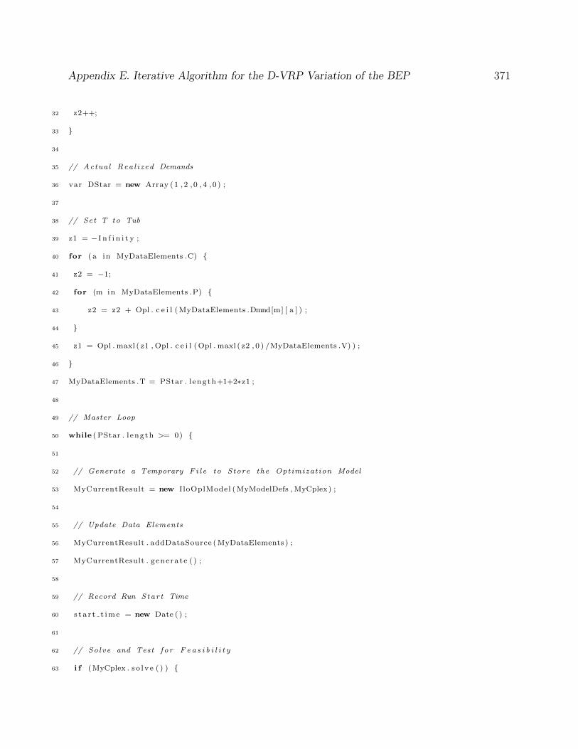
Appendix E. Iterative Algorithm for the D-VRP Variation of the BEP 371
32 z2++;
33 }
34
35 // Actual Rea l i zed Demands
36 var DStar = new Array (1 , 2 , 0 , 4 , 0 ) ;
37
38 // Set T to Tub
39 z1 = − I n f i n i t y ;
40 for ( a in MyDataElements .C) {
41 z2 = −1;
42 for (m in MyDataElements .P) {
43 z2 = z2 + Opl . c e i l ( MyDataElements .Dmnd[m] [ a ] ) ;
44 }
45 z1 = Opl . maxl ( z1 , Opl . c e i l ( Opl . maxl ( z2 , 0 ) /MyDataElements .V) ) ;
46 }
47 MyDataElements .T = PStar . l ength+1+2∗z1 ;
48
49 // Master Loop
50 while ( PStar . l ength >= 0) {
51
52 // Generate a Temporary F i l e to Store the Optimizat ion Model
53 MyCurrentResult = new I loOplModel ( MyModelDefs , MyCplex ) ;
54
55 // Update Data Elements
56 MyCurrentResult . addDataSource ( MyDataElements ) ;
57 MyCurrentResult . generate ( ) ;
58
59 // Record Run S tar t Time
60 s t a r t t i m e = new Date ( ) ;
61
62 // So lve and Test f o r F e a s i b i l i t y
63 i f (MyCplex . s o l v e ( ) ) {

Appendix E. Iterative Algorithm for the D-VRP Variation of the BEP 372
64
65 // Record Run End−Time
66 end time = new Date ( ) ;
67
68 // Invoke the PostProcess Method
69 MyCurrentResult . pos tProces s ( ) ;
70
71 // Exi t i f A l l Uncertainty Resolved
72 i f ( PStar . l ength == 0) break ;
73
74 // Output I t e r a t i o n Data to the Sc r i p t Log Window
75 w r i t e l n ( ” I t e r a t i o n : ” , MyDataElements . ConstrainedT ) ;
76 w r i t e l n ( ”Expected Total Travel Time : ” ,MyCplex . getObjValue ( ) ) ;
77 w r i t e l n ( ” So lu t i on Time : ” , ( end time . getTime ( )−s t a r t t i m e . getTime ( ) ) /1000 , ” seconds ” ) ;
78 w r i t e l n ( ) ;
79 w r i t e l n ( ”Bus” , ”\ t ” , ” Traver sa l ” , ”\ t ” , ”Arc” , ”\ t ” , ”Loading” ) ;
80
81 for ( a in MyCurrentResult .A) {
82 for (m=1;m<=MyCurrentResult .V;m++){
83 i f ( MyCurrentResult . x [ a ] [m] [ MyDataElements . ConstrainedT ] [ Opl . f i r s t ( MyDataElements .C) ] ==
1) {
84
85 nLoad = ”−”
86
87 // Save the Common Arc Traversa l to Set Rˆ∗
88 MyDataElements . R Star . add ( a ,m, MyDataElements . ConstrainedT ) ;
89
90 // Determine i f the Des t ina t ion Node i s in Set Pˆ∗
91 bFound = 0 ;
92 for ( z1 =0;z1<=PStar . length −1; z1++) {
93 i f ( PStar [ z1 ] == a . des t ) {
94 bFound = 1 ;
Appendix E. Iterative Algorithm for the D-VRP Variation of the BEP 373
95 break ;
96 }
97 }
98 i f (bFound == 1) {
99
100 // Set the Respec t i ve Location−Scenarios with the Rea l i zed Demand
101 for ( z2 in MyCurrentResult .C) {
102
103 // Find the Corresponding DStar Element
104 for ( z3 =0;z3<=JStar . length −1; z3++) {
105 i f ( z2 . des t == JStar [ z3 ] ) {
106 i f ( MyDataElements .Dmnd[ a . des t ] [ z2 ] == DStar [ z3 ] ) {
107 // Add Des t ina t ion to Set C Star
108 nLoad = MyCurrentResult . y [ a . des t ] [m] [ MyDataElements . ConstrainedT ] [ z2 ] ;
109 MyDataElements . C Star . add ( a . dest ,m, MyDataElements . ConstrainedT , nLoad ) ;
110 } else {
111 MyDataElements .Dmnd[ a . des t ] [ z2 ] = DStar [ z3 ] ;
112 }
113 break ;
114 }
115 }
116 }
117
118 // Remove the Corresponding Element from Set Pˆ∗
119 d e l e t e PStar [ z1 ] ;
120
121 } else {
122
123 // Determine i f the d e s t i na t i on node i s in Set P
124 for ( z1 in MyDataElements .P) {
125 i f ( a . des t == z1 ) {
126 // Add Des t ina t ion to Set C Star

Appendix E. Iterative Algorithm for the D-VRP Variation of the BEP 374
127 nLoad = MyCurrentResult . y [ a . des t ] [m] [ MyDataElements . ConstrainedT ] [ Opl . f i r s t (
MyDataElements .C) ] ;
128 MyDataElements . C Star . add ( a . dest ,m, MyDataElements . ConstrainedT , nLoad ) ;
129 break ;
130 }
131 }
132 }
133
134 // Output Arc Traversa l Data to the Sc r i p t Log Window
135 w r i t e l n (m, ”\ t ” , MyDataElements . ConstrainedT , ”\ t ” , a , ”\ t ” , nLoad ) ;
136 }
137 }
138 }
139
140 // Update So lu t i on Timer
141 end time = new Date ( ) ;
142 w r i t e l n ( ) ;
143 w r i t e l n ( ” So lu t i on + Proce s s ing Time : ” , ( end time . getTime ( )−s t a r t t i m e . getTime ( ) ) /1000 , ”
seconds ” ) ;
144 w r i t e l n ( ) ;
145 w r i t e l n ( ”−−−−−−−−−−−−−−−−−−−−−−−−−−−−−−−−−−−−−−” ) ;
146 w r i t e l n ( ) ;
147
148 // Increment t ˆ∗
149 MyDataElements . ConstrainedT = MyDataElements . ConstrainedT +1;
150
151 } else {
152
153 // Output Error Flag to the Sc r i p t Log Window
154 end time = new Date ( ) ;
155 w r i t e l n ( ) ;
156 w r i t e l n ( ”An Error Occurred” ) ;
Appendix E. Iterative Algorithm for the D-VRP Variation of the BEP 375
157 w r i t e l n ( ) ;
158 w r i t e l n ( ”Time : ” , ( end time . getTime ( )−s t a r t t i m e . getTime ( ) ) /1000 , ” seconds ” ) ;
159 w r i t e l n ( ” Best Object ive Function Value : ” ,MyCplex . GetBestObjValue ( ) ) ;
160 w r i t e l n ( ”MIP Gap = ” , ( MyCplex . getBestObjValue ( )−MyCplex . getObjValue ( ) ) /(1 e−10+MyCplex .
getObjValue ( ) ) ) ;
161
162 bError = 1 ;
163 break ;
164 }
165 }
166
167 // Record Run Overa l l Completion Time
168 o v e r a l l e n d t i m e = new Date ( ) ;
169
170 // Output Fina l Routes to the Sc r i p t Log Window
171 i f ( bError == 0) {
172 w r i t e l n ( ”Run Fin i shed . F ina l Tour : ” ) ;
173 w r i t e l n ( )
174 w r i t e l n ( ”Bus” , ”\ t ” , ” Traver sa l ” , ”\ t ” , ”Arc” , ”\ t ” , ”Loading” ) ;
175 for (m=1;m<=MyCurrentResult .V;m++){
176 for ( z1 =1;z1<=MyCurrentResult .T; z1++) {
177 for ( a in MyCurrentResult .A) {
178 i f ( MyCurrentResult . x [ a ] [m] [ z1 ] [ Opl . f i r s t ( MyCurrentResult .C) ] == 1) {
179 bFound = 0 ;
180 for ( z2 in MyDataElements .P) {
181 i f ( z2 == a . des t ) {
182 bFound = 1 ;
183 break ;
184 }
185 }
186 i f (bFound == 1) {
Appendix E. Iterative Algorithm for the D-VRP Variation of the BEP 376
187 w r i t e l n (m, ”\ t ” , z1 , ”\ t ” , a , ”\ t ” , MyCurrentResult . y [ a . des t ] [m] [ z1 ] [ Opl . f i r s t (
MyCurrentResult .C) ] ) ;
188 } else {
189 w r i t e l n (m, ”\ t ” , z1 , ”\ t ” , a , ”\ t ” , ”−” ) ;
190 }
191 }
192 }
193 }
194 }
195 w r i t e l n ( ) ;
196 w r i t e l n ( ” Rea l i zed Total Travel Time : ” ,MyCplex . getObjValue ( ) ) ;
197 w r i t e l n ( ” So lu t i on + Proce s s ing Time : ” , ( o v e r a l l e n d t i m e . getTime ( )−s t a r t t i m e . getTime ( ) )
/1000 , ” seconds ” ) ;
198 w r i t e l n ( ) ;
199 w r i t e l n ( ” Overa l l So lu t i on Time : ” , ( o v e r a l l e n d t i m e . getTime ( )−o v e r a l l s t a r t t i m e . getTime ( ) )
/1000 , ” seconds ” ) ;
200 }
201 // Release Remaining Objec t s
202 MyCplex . end ( ) ;
203 MyModelDefs . end ( ) ;
204 MyResult . end ( ) ;
205 MyDataElements . end ( ) ;
206 MyCurrentResult . end ( ) ;
207 }
Appendix E. Iterative Algorithm for the D-VRP Variation of the BEP 377
E.2 Deterministic Formulation
E.2.1 Model File (EnhancedModel.mod)
1 // MODEL FILE
2
3 // Import Network Parameters
4 { s t r i n g } S = . . . ; // Set o f Depots
5 { s t r i n g } P = . . . ; // Set o f Pick−up Locat ions
6 { s t r i n g } N =(S union P) ; // Set o f Nodes
7 { s t r i n g } PStar = . . . ; // Set o f Unv i s i t ed Pick−up Locat ions
8 { s t r i n g } C = . . . ; // Set o f Scenarios
9
10 tup l e Arcs { s t r i n g o r i g ; s t r i n g dest ; } ; // Set o f Arcs
11 {Arcs} A with o r i g in N, des t in N = . . . ;
12
13 tup l e Demand { s t r i n g dest ; s t r i n g s c e n a r i o ; f loat Value ; } ; // Set o f Demands
14 {Demand} D = . . . ;
15
16 int V = . . . ; // F l e e t S i ze Ava i l a b l e
17 range VRange = 1 . .V;
18
19 f loat time [A] = . . . ; // Arc Traversa l Times
20 f loat Dmnd[P] = . . . ; // Lowest Po s s i b l e Demand Rea l i z a t i on s
21 int ConstrainedT = . . . ; // I t e r a t i o n Number
22
23 // Determine the Upper Bound on T
24 int T = . . . ;
25 range TRange = 1 . .T;
26
27 // Set o f Previous Arc Traversa l s
28 tup l e rSta r {Arcs arc ; int v e h i c l e ; int t r a v e r s a l ; } ;
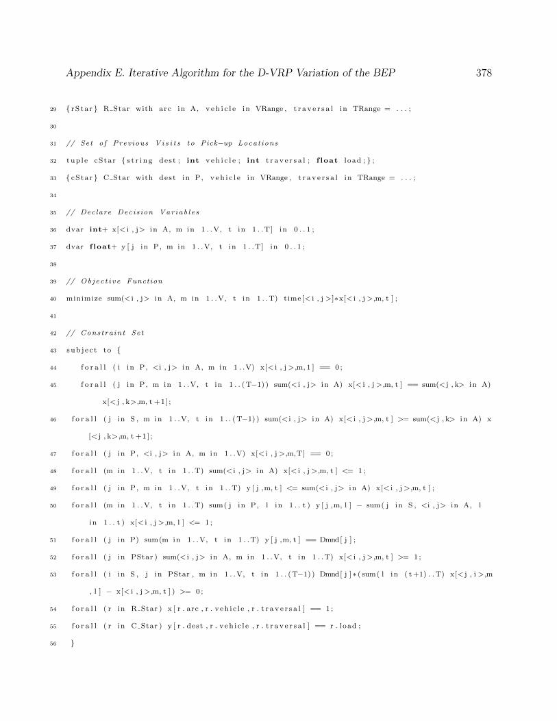
Appendix E. Iterative Algorithm for the D-VRP Variation of the BEP 378
29 { rS ta r } R Star with arc in A, v e h i c l e in VRange , t r a v e r s a l in TRange = . . . ;
30
31 // Set o f Previous V i s i t s to Pick−up Locat ions
32 tup l e cStar { s t r i n g dest ; int v e h i c l e ; int t r a v e r s a l ; f loat load ; } ;
33 { cStar } C Star with dest in P, v e h i c l e in VRange , t r a v e r s a l in TRange = . . . ;
34
35 // Declare Decis ion Var iab l e s
36 dvar int+ x[< i , j> in A, m in 1 . .V, t in 1 . .T] in 0 . . 1 ;
37 dvar f loat+ y [ j in P, m in 1 . .V, t in 1 . .T] in 0 . . 1 ;
38
39 // Ob j ec t i v e Function
40 minimize sum(< i , j> in A, m in 1 . .V, t in 1 . .T) time [< i , j >]∗x[< i , j>,m, t ] ;
41
42 // Constra int Set
43 s ub j e c t to {
44 f o r a l l ( i in P, <i , j> in A, m in 1 . .V) x[< i , j>,m, 1 ] == 0 ;
45 f o r a l l ( j in P, m in 1 . .V, t in 1 . . ( T−1) ) sum(< i , j> in A) x[< i , j>,m, t ] == sum(< j , k> in A)
x[< j , k>,m, t +1] ;
46 f o r a l l ( j in S , m in 1 . .V, t in 1 . . ( T−1) ) sum(< i , j> in A) x[< i , j>,m, t ] >= sum(< j , k> in A) x
[< j , k>,m, t +1] ;
47 f o r a l l ( j in P, <i , j> in A, m in 1 . .V) x[< i , j>,m,T] == 0 ;
48 f o r a l l (m in 1 . .V, t in 1 . .T) sum(< i , j> in A) x[< i , j>,m, t ] <= 1 ;
49 f o r a l l ( j in P, m in 1 . .V, t in 1 . .T) y [ j ,m, t ] <= sum(< i , j> in A) x[< i , j>,m, t ] ;
50 f o r a l l (m in 1 . .V, t in 1 . .T) sum( j in P, l in 1 . . t ) y [ j ,m, l ] − sum( j in S , <i , j> in A, l
in 1 . . t ) x[< i , j>,m, l ] <= 1 ;
51 f o r a l l ( j in P) sum(m in 1 . .V, t in 1 . .T) y [ j ,m, t ] == Dmnd[ j ] ;
52 f o r a l l ( j in PStar ) sum(< i , j> in A, m in 1 . .V, t in 1 . .T) x[< i , j>,m, t ] >= 1 ;
53 f o r a l l ( i in S , j in PStar , m in 1 . .V, t in 1 . . ( T−1) ) Dmnd[ j ] ∗ ( sum( l in ( t+1) . . T) x[< j , i >,m
, l ] − x[< i , j>,m, t ] ) >= 0 ;
54 f o r a l l ( r in R Star ) x [ r . arc , r . v eh i c l e , r . t r a v e r s a l ] == 1 ;
55 f o r a l l ( r in C Star ) y [ r . dest , r . v eh i c l e , r . t r a v e r s a l ] == r . load ;
56 }
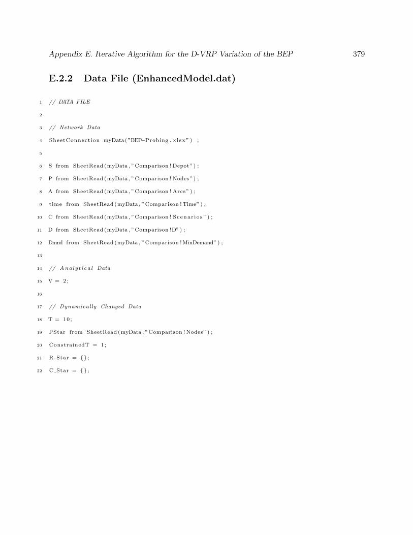
Appendix E. Iterative Algorithm for the D-VRP Variation of the BEP 379
E.2.2 Data File (EnhancedModel.dat)
1 // DATA FILE
2
3 // Network Data
4 SheetConnection myData( ”BEP−Probing . x l sx ” ) ;
5
6 S from SheetRead (myData , ”Comparison ! Depot” ) ;
7 P from SheetRead (myData , ”Comparison ! Nodes” ) ;
8 A from SheetRead (myData , ”Comparison ! Arcs” ) ;
9 time from SheetRead (myData , ”Comparison ! Time” ) ;
10 C from SheetRead (myData , ”Comparison ! Scenar i o s ” ) ;
11 D from SheetRead (myData , ”Comparison !D” ) ;
12 Dmnd from SheetRead (myData , ”Comparison ! MinDemand” ) ;
13
14 // Ana l y t i c a l Data
15 V = 2 ;
16
17 // Dynamically Changed Data
18 T = 10 ;
19 PStar from SheetRead (myData , ”Comparison ! Nodes” ) ;
20 ConstrainedT = 1 ;
21 R Star = {} ;
22 C Star = {} ;
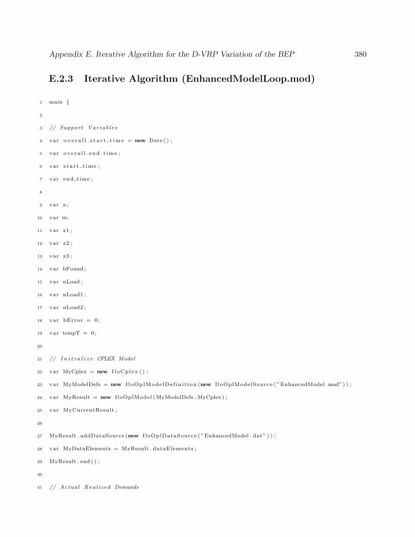
Appendix E. Iterative Algorithm for the D-VRP Variation of the BEP 380
E.2.3 Iterative Algorithm (EnhancedModelLoop.mod)
1 main {
2
3 // Support Var iab l e s
4 var o v e r a l l s t a r t t i m e = new Date ( ) ;
5 var o v e r a l l e n d t i m e ;
6 var s t a r t t i m e ;
7 var end time ;
8
9 var a ;
10 var m;
11 var z1 ;
12 var z2 ;
13 var z3 ;
14 var bFound ;
15 var nLoad ;
16 var nLoad1 ;
17 var nLoad2 ;
18 var bError = 0 ;
19 var tempT = 0 ;
20
21 // I n i t i a l i z e CPLEX Model
22 var MyCplex = new I l oCp lex ( ) ;
23 var MyModelDefs = new I l oOp lMode lDe f in i t i on (new I loOplModelSource ( ”EnhancedModel .mod” ) ) ;
24 var MyResult = new I loOplModel ( MyModelDefs , MyCplex ) ;
25 var MyCurrentResult ;
26
27 MyResult . addDataSource (new I loOplDataSource ( ”EnhancedModel . dat” ) ) ;
28 var MyDataElements = MyResult . dataElements ;
29 MyResult . end ( ) ;
30
31 // Actual Rea l i zed Demands
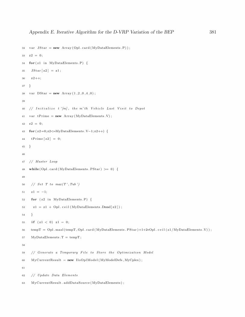
Appendix E. Iterative Algorithm for the D-VRP Variation of the BEP 381
32 var JStar = new Array ( Opl . card ( MyDataElements .P) ) ;
33 z2 = 0 ;
34 for ( z1 in MyDataElements .P) {
35 JStar [ z2 ] = z1 ;
36 z2++;
37 }
38 var DStar = new Array (1 , 2 , 0 , 4 , 0 ) ;
39
40 // I n i t i a l i z e t ’ [m] , the mˆ th Vehic le Last V i s i t to Depot
41 var tPrime = new Array ( MyDataElements .V) ;
42 z2 = 0 ;
43 for ( z2 =0;z2<=MyDataElements .V−1; z2++) {
44 tPrime [ z2 ] = 0 ;
45 }
46
47 // Master Loop
48 while ( Opl . card ( MyDataElements . PStar ) >= 0) {
49
50 // Set T to max(T ’ ,Tub ’)
51 z1 = −1;
52 for ( z2 in MyDataElements .P) {
53 z1 = z1 + Opl . c e i l ( MyDataElements .Dmnd[ z2 ] ) ;
54 }
55 i f ( z1 < 0) z1 = 0 ;
56 tempT = Opl . maxl (tempT , Opl . card ( MyDataElements . PStar )+1+2∗Opl . c e i l ( z1/MyDataElements .V) ) ;
57 MyDataElements .T = tempT ;
58
59 // Generate a Temporary F i l e to Store the Optimizat ion Model
60 MyCurrentResult = new I loOplModel ( MyModelDefs , MyCplex ) ;
61
62 // Update Data Elements
63 MyCurrentResult . addDataSource ( MyDataElements ) ;
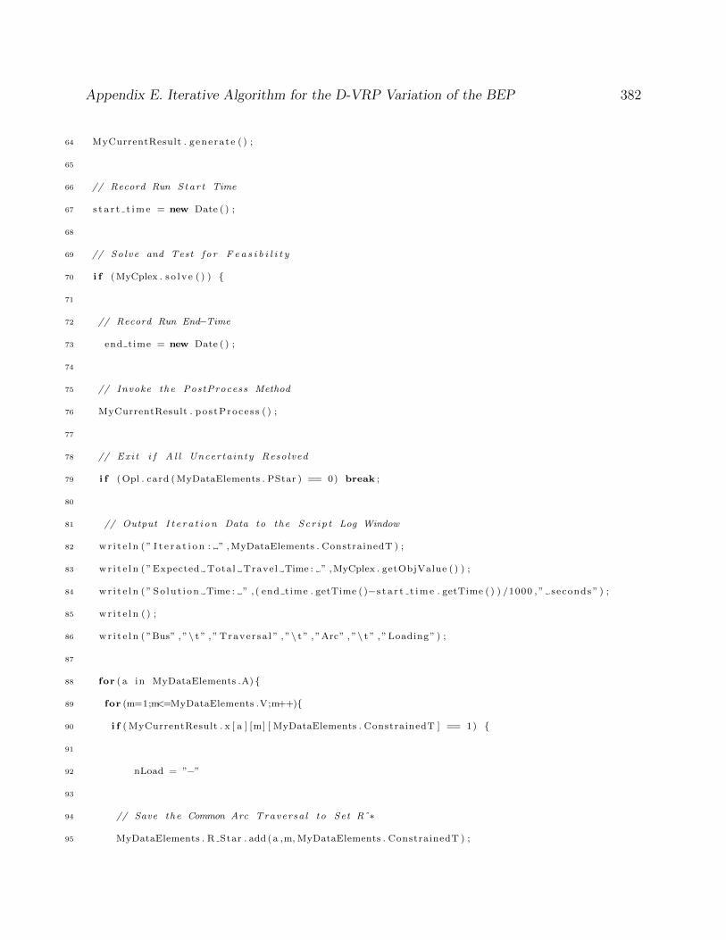
Appendix E. Iterative Algorithm for the D-VRP Variation of the BEP 382
64 MyCurrentResult . generate ( ) ;
65
66 // Record Run S tar t Time
67 s t a r t t i m e = new Date ( ) ;
68
69 // So lve and Test f o r F e a s i b i l i t y
70 i f (MyCplex . s o l v e ( ) ) {
71
72 // Record Run End−Time
73 end time = new Date ( ) ;
74
75 // Invoke the PostProcess Method
76 MyCurrentResult . pos tProces s ( ) ;
77
78 // Exi t i f A l l Uncertainty Resolved
79 i f ( Opl . card ( MyDataElements . PStar ) == 0) break ;
80
81 // Output I t e r a t i o n Data to the Sc r i p t Log Window
82 w r i t e l n ( ” I t e r a t i o n : ” , MyDataElements . ConstrainedT ) ;
83 w r i t e l n ( ”Expected Total Travel Time : ” ,MyCplex . getObjValue ( ) ) ;
84 w r i t e l n ( ” So lu t i on Time : ” , ( end time . getTime ( )−s t a r t t i m e . getTime ( ) ) /1000 , ” seconds ” ) ;
85 w r i t e l n ( ) ;
86 w r i t e l n ( ”Bus” , ”\ t ” , ” Traver sa l ” , ”\ t ” , ”Arc” , ”\ t ” , ”Loading” ) ;
87
88 for ( a in MyDataElements .A) {
89 for (m=1;m<=MyDataElements .V;m++){
90 i f ( MyCurrentResult . x [ a ] [m] [ MyDataElements . ConstrainedT ] == 1) {
91
92 nLoad = ”−”
93
94 // Save the Common Arc Traversa l to Set Rˆ∗
95 MyDataElements . R Star . add ( a ,m, MyDataElements . ConstrainedT ) ;
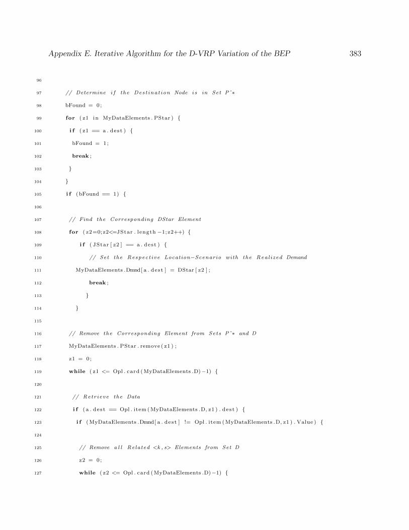
Appendix E. Iterative Algorithm for the D-VRP Variation of the BEP 383
96
97 // Determine i f the Des t ina t ion Node i s in Set Pˆ∗
98 bFound = 0 ;
99 for ( z1 in MyDataElements . PStar ) {
100 i f ( z1 == a . des t ) {
101 bFound = 1 ;
102 break ;
103 }
104 }
105 i f (bFound == 1) {
106
107 // Find the Corresponding DStar Element
108 for ( z2 =0;z2<=JStar . length −1; z2++) {
109 i f ( JStar [ z2 ] == a . des t ) {
110 // Set the Respec t i ve Location−Scenario with the Rea l i zed Demand
111 MyDataElements .Dmnd[ a . des t ] = DStar [ z2 ] ;
112 break ;
113 }
114 }
115
116 // Remove the Corresponding Element from Sets Pˆ∗ and D
117 MyDataElements . PStar . remove ( z1 ) ;
118 z1 = 0 ;
119 while ( z1 <= Opl . card ( MyDataElements .D)−1) {
120
121 // Retr i eve the Data
122 i f ( a . des t == Opl . item ( MyDataElements .D, z1 ) . des t ) {
123 i f ( MyDataElements .Dmnd[ a . des t ] != Opl . item ( MyDataElements .D, z1 ) . Value ) {
124
125 // Remove a l l Related <k , s> Elements from Set D
126 z2 = 0 ;
127 while ( z2 <= Opl . card ( MyDataElements .D)−1) {
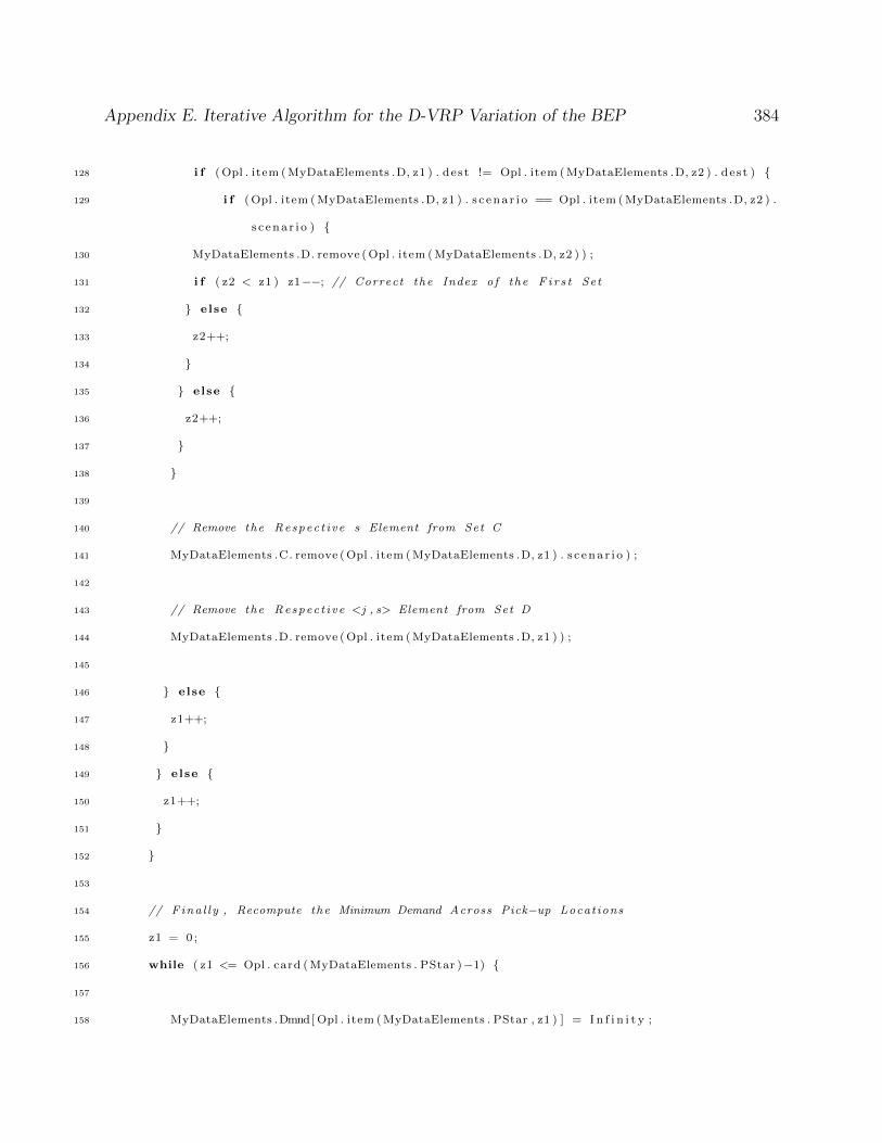
Appendix E. Iterative Algorithm for the D-VRP Variation of the BEP 384
128 i f ( Opl . item ( MyDataElements .D, z1 ) . des t != Opl . item ( MyDataElements .D, z2 ) . des t ) {
129 i f ( Opl . item ( MyDataElements .D, z1 ) . s c e n a r i o == Opl . item ( MyDataElements .D, z2 ) .
s c e n a r i o ) {
130 MyDataElements .D. remove ( Opl . item ( MyDataElements .D, z2 ) ) ;
131 i f ( z2 < z1 ) z1−−; // Correct the Index o f the F i r s t Set
132 } else {
133 z2++;
134 }
135 } else {
136 z2++;
137 }
138 }
139
140 // Remove the Respec t i ve s Element from Set C
141 MyDataElements .C. remove ( Opl . item ( MyDataElements .D, z1 ) . s c e n a r i o ) ;
142
143 // Remove the Respec t i ve <j , s> Element from Set D
144 MyDataElements .D. remove ( Opl . item ( MyDataElements .D, z1 ) ) ;
145
146 } else {
147 z1++;
148 }
149 } else {
150 z1++;
151 }
152 }
153
154 // Fina l l y , Recompute the Minimum Demand Across Pick−up Locat ions
155 z1 = 0 ;
156 while ( z1 <= Opl . card ( MyDataElements . PStar )−1) {
157
158 MyDataElements .Dmnd[ Opl . item ( MyDataElements . PStar , z1 ) ] = I n f i n i t y ;
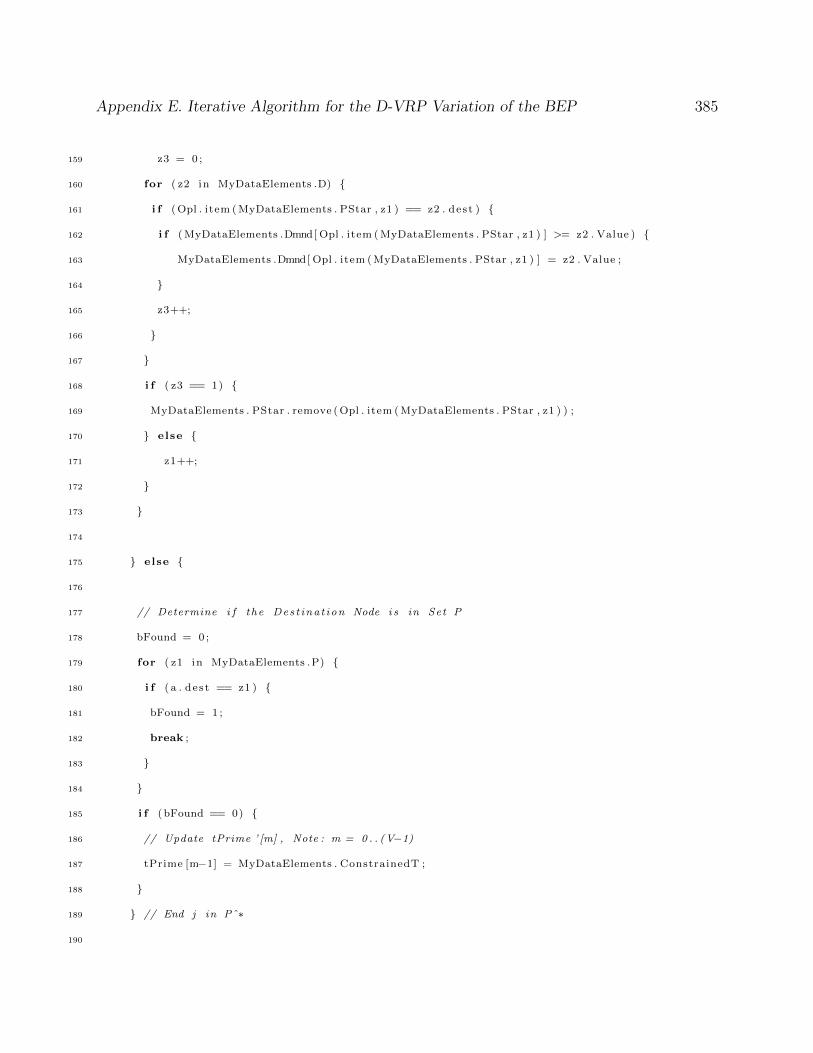
Appendix E. Iterative Algorithm for the D-VRP Variation of the BEP 385
159 z3 = 0 ;
160 for ( z2 in MyDataElements .D) {
161 i f ( Opl . item ( MyDataElements . PStar , z1 ) == z2 . des t ) {
162 i f ( MyDataElements .Dmnd[ Opl . item ( MyDataElements . PStar , z1 ) ] >= z2 . Value ) {
163 MyDataElements .Dmnd[ Opl . item ( MyDataElements . PStar , z1 ) ] = z2 . Value ;
164 }
165 z3++;
166 }
167 }
168 i f ( z3 == 1) {
169 MyDataElements . PStar . remove ( Opl . item ( MyDataElements . PStar , z1 ) ) ;
170 } else {
171 z1++;
172 }
173 }
174
175 } else {
176
177 // Determine i f the Des t ina t ion Node i s in Set P
178 bFound = 0 ;
179 for ( z1 in MyDataElements .P) {
180 i f ( a . des t == z1 ) {
181 bFound = 1 ;
182 break ;
183 }
184 }
185 i f (bFound == 0) {
186 // Update tPrime ’ [m] , Note : m = 0 . . (V−1)
187 tPrime [m−1] = MyDataElements . ConstrainedT ;
188 }
189 } // End j in Pˆ∗
190

Appendix E. Iterative Algorithm for the D-VRP Variation of the BEP 386
191 // Manually Compute the Loading at the Vehic le
192 i f (bFound == 1) {
193 nLoad1 = 1 ;
194 for ( z2 in MyDataElements .P) {
195 for ( z3=tPrime [m−1]+1; z3<=MyDataElements . ConstrainedT ; z3++) {
196 nLoad1 = nLoad1 − MyCurrentResult . y [ z2 ] [m] [ z3 ] ;
197 }
198 }
199 nLoad2 = MyDataElements .Dmnd[ a . des t ] ;
200 for ( z2 =1;z2<=m; z2++) {
201 nLoad2 = nLoad2 − MyCurrentResult . y [ a . des t ] [ z2 ] [ MyDataElements . ConstrainedT ] ;
202 }
203 nLoad = MyCurrentResult . y [ a . des t ] [m] [ MyDataElements . ConstrainedT ]+Opl . minl ( nLoad1 ,
nLoad2 ) ;
204 MyDataElements . C Star . add ( a . dest ,m, MyDataElements . ConstrainedT , nLoad ) ;
205 }
206
207 // Output Arc Traversa l Data to the Sc r i p t Log Window
208 w r i t e l n (m, ”\ t ” , MyDataElements . ConstrainedT , ”\ t ” , a , ”\ t ” , nLoad ) ;
209
210 } // End x i j ˆmtf == 1?
211 } // Next m = 1 , . . . ,V
212 } // Next ( i , j ) in A
213
214 // Update So lu t i on Timer
215 end time = new Date ( ) ;
216 w r i t e l n ( ) ;
217 w r i t e l n ( ” So lu t i on + Proce s s ing Time : ” , ( end time . getTime ( )−s t a r t t i m e . getTime ( ) ) /1000 , ”
seconds ” ) ;
218 w r i t e l n ( ) ;
219 w r i t e l n ( ”−−−−−−−−−−−−−−−−−−−−−−−−−−−−−−−−−−−−−−” ) ;
220 w r i t e l n ( ) ;

Appendix E. Iterative Algorithm for the D-VRP Variation of the BEP 387
221
222 // Increment t ˆ∗
223 MyDataElements . ConstrainedT = MyDataElements . ConstrainedT +1;
224
225 // Release the MyCurrentResult Object , b e f o r e r e i n i t i a t i n g i t
226 MyCurrentResult . end ( ) ;
227
228 } else {
229
230 // Output Error Flag to the Sc r i p t Log Window
231 end time = new Date ( ) ;
232 w r i t e l n ( ) ;
233 w r i t e l n ( ”An Error Occurred” ) ;
234 w r i t e l n ( ) ;
235 w r i t e l n ( ”Time : ” , ( end time . getTime ( )−s t a r t t i m e . getTime ( ) ) /1000 , ” seconds ” ) ;
236 w r i t e l n ( ” Best Object ive Function Value : ” ,MyCplex . GetBestObjValue ( ) ) ;
237 w r i t e l n ( ”MIP Gap = ” , ( MyCplex . getBestObjValue ( )−MyCplex . getObjValue ( ) ) /(1 e−10+MyCplex .
getObjValue ( ) ) ) ;
238
239 bError = 1 ;
240 break ;
241
242 } // End Optimize
243 } // Next Loop
244
245 // Record Run Overa l l Completion Time
246 o v e r a l l e n d t i m e = new Date ( ) ;
247
248 // Output Fina l Routes to the Sc r i p t Log Window
249 i f ( bError == 0) {
250 w r i t e l n ( ”Run Fin i shed . F ina l Tour : ” ) ;
251 w r i t e l n ( )

Appendix E. Iterative Algorithm for the D-VRP Variation of the BEP 388
252 w r i t e l n ( ”Bus” , ”\ t ” , ” Traver sa l ” , ”\ t ” , ”Arc” , ”\ t ” , ”Loading” ) ;
253 for (m=1;m<=MyDataElements .V;m++){
254 for ( z1 =1;z1<=MyCurrentResult .T; z1++) {
255 for ( a in MyDataElements .A) {
256 i f ( MyCurrentResult . x [ a ] [m] [ z1 ] == 1) {
257 bFound = 0 ;
258 for ( z2 in MyDataElements .P) {
259 i f ( z2 == a . des t ) {
260 bFound = 1 ;
261 break ;
262 }
263 }
264 i f (bFound == 1) {
265 w r i t e l n (m, ”\ t ” , z1 , ”\ t ” , a , ”\ t ” , MyCurrentResult . y [ a . des t ] [m] [ z1 ] ) ;
266 } else {
267 w r i t e l n (m, ”\ t ” , z1 , ”\ t ” , a , ”\ t ” , ”−” ) ;
268 }
269 }
270 }
271 }
272 }
273 w r i t e l n ( ) ;
274 w r i t e l n ( ” Rea l i zed Total Travel Time : ” ,MyCplex . getObjValue ( ) ) ;
275 w r i t e l n ( ” So lu t i on + Proce s s ing Time : ” , ( o v e r a l l e n d t i m e . getTime ( )−s t a r t t i m e . getTime ( ) )
/1000 , ” seconds ” ) ;
276 w r i t e l n ( ) ;
277 w r i t e l n ( ” Overa l l So lu t i on Time : ” , ( o v e r a l l e n d t i m e . getTime ( )−o v e r a l l s t a r t t i m e . getTime ( ) )
/1000 , ” seconds ” ) ;
278 }
279 // Release Remaining Objec t s
280 MyCplex . end ( ) ;
281 MyModelDefs . end ( ) ;
Appendix E. Iterative Algorithm for the D-VRP Variation of the BEP 389
282 MyDataElements . end ( ) ;
283 MyCurrentResult . end ( ) ;
284 }