vegard stürzinger

Faculty of Bioscience, Fisheries, and Economics, Department for Arctic and Marine Biology

Let it glow! Adapting a method to detect microplastics in snow and

evaluate the potential for long-range transport

Vegard Stürzinger

Master’s thesis in Biology, BIO3950, May 2020

i

Master student: Vegard Stürzinger1,2,3

Main supervisor: Sophie Bourgeon1

Co-supervisor: Ingeborg Hallanger2

Co-supervisor: Dorte Hertzke3

Internal sensor: Anita Evenset4

External sensor: Mats Bjørkman5

1 University in Tromsø, 2 Norwegian Polar Institute, 3 Norwegian Institute for Air

Research, 4 Akvaplan NIVA, 5 University of Gothenburg

iii

Acknowledgments

First and foremost, I would like to express my gratitude to my supervisors, Sophie Bourgeon,

Ingeborg Hallanger, and Dorte Hertzke. They guided me through my master thesis, even in

trying times, and provided me with an opportunity to go to China to meet my Chinese

counterparts. I would like to thank J-C Gallet for his advice on snow sampling and providing

me with tips and equipment. Special mentions to Ivan for helping me with sampling the snow

and Mathea for supporting me even though I was going through darker times in my life.

Thank you for the ride to my friends who have been writing their thesis alongside me. I am

grateful to the Norwegian Polar Institute for providing an office with great people for lunches,

sporadic help, and Friday beers. A big thank you to the Norwegian Institute for Air Research,

Tromsø for providing me with laboratory facilities and knowledge that helped me along the

way. Finally, a mention to Geir W. Gabrielsen for introducing me to Ingeborg for this master

thesis.

v

Abstract

Harmonization of methods in microplastics research is lacking; this is affecting the

comparability of results and hindering reproducibility. Investigating microplastics in snow is a

relatively new field of research, and it can be used to answer questions about long-range

atmospheric transport of microplastics. In this thesis, snow sampling methods were combined

with the dye, Nile Red, to develop a method to identify and quantify microplastics in snow.

There was an emphasis on quality control and quality assurance, and blank samples were

taken throughout the sampling and laboratory procedures. To test and validate the method, a

study was performed in northern Norway to compare urban and rural locations. In addition to

the field samples, laboratory testing was done by staining know plastic polymers and

excluding possible staining of different organic material occurring in snow. We found that the

urban locations contained a significantly higher mean number of microplastics per liter of

snow compared to rural locations, 694 ± 375 (mean ± S.E.) particles L-1 snow vs. 432 ± 386

particles L-1 snow, respectively. The most substantial proportion of microplastics was in the

lowest size class (22-50 µm) for both rural and urban locations. This protocol provides a

simple and effective method that can be applied anywhere and could increase the

comparability of results.

Keywords: Nile Red, Quality Assurance, Protocol development, Arctic, Stereomicroscope.

vii

List of abbreviations

LED - Light Emitting Diodes

NR - Nile Red

MP - Microplastic

WP550 - Whirl-Pak 550

LRT – Long-range transport

MDL – Method detection limit

FTIR - Fourier transform infrared spectroscopy

SD – Standard deviation

DD – Decimal degrees

QA – Quality Assurance

QC – Quality Control

ix

Table of contents

Acknowledgments ................................................................................................................ iii

Abstract ................................................................................................................................. v

List of abbreviations ............................................................................................................ vii

Table of contents .................................................................................................................. ix

1 Introduction ................................................................................................................... 1

1.1 Plastic pollution- sources and size classes of particles ...............................................1

1.2 Pathways ..................................................................................................................3

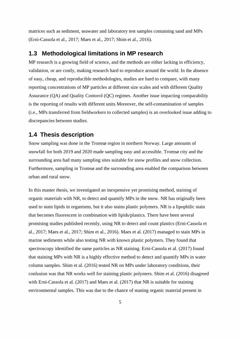
1.3 Methodological limitations in MP research ...............................................................5

1.4 Thesis description .....................................................................................................5

2 Materials and methods ................................................................................................... 7

2.1 Sampling strategy .....................................................................................................7

2.2 Sampling locations ...................................................................................................7

2.3 QA and QC in the field .............................................................................................9

2.4 Snow pits and physical parameters ...........................................................................9

2.5 Thawing of snow samples....................................................................................... 12

2.6 Preparation of equipment for cleanroom ................................................................. 12

2.7 Preparation of NR solution ..................................................................................... 12

2.8 Filtration and staining of melted snow .................................................................... 13

2.9 QA and QC sampling and sample treatment ........................................................... 14

2.10 The method detection limit (MDL) ..................................................................... 14

2.11 Visual analysis .................................................................................................... 15

2.12 Image analysis .................................................................................................... 15

2.13 Comparing manual and automated counting ........................................................ 16

2.14 Data frame and correction ................................................................................... 16

x

2.14.1 Correcting for snow density ............................................................................. 16

2.14.2 Calculating particle size................................................................................... 16

2.15 Statistical analysis and data processing ............................................................... 17

3 Development of protocol ............................................................................................. 18

3.1 Snow sampling ....................................................................................................... 18

3.2 QA and QC in the field ........................................................................................... 18

3.3 Storage and handling of snow samples ................................................................... 19

3.4 Solvent and Nile red concentration ......................................................................... 19

3.5 Stereomicroscope modification ............................................................................... 19

3.6 Staining of plastic and possible artifacts ................................................................. 20

3.7 Establishing aliquot volume based on NR trials ...................................................... 21

3.8 Filtration and staining of samples ........................................................................... 21

3.9 QA and QC in the laboratory .................................................................................. 21

3.10 Counting of microplastics ................................................................................... 22

4 Results ......................................................................................................................... 23

4.1 The occurrence of MP particles .............................................................................. 23

4.2 The difference in MP sizes between urban and rural sampling sites ........................ 26

4.3 Viability of the method ........................................................................................... 28

4.3.1 Field blanks and MDL ..................................................................................... 28

4.3.2 Comparing manual count to automatic count ................................................... 29

4.3.3 Background noise in images ............................................................................ 30

5 Discussion ................................................................................................................... 31

5.1 Method adaptation .................................................................................................. 32

5.1.1 Internal suitability of NR staining .................................................................... 32

5.1.2 Determination of the MP count ........................................................................ 33

5.1.3 Comparability with other MP detection methods ............................................. 33

xi

5.2 Application of the method for the determination of MPs in snow ............................ 34

5.2.1 Amount of microplastics in rural and urban areas ............................................ 34

5.2.2 Size classes of MP particles in urban and rural stations .................................... 36

5.3 Study conclusion .................................................................................................... 36

5.4 Perspective for future research and practice ............................................................ 37

6 Conclusion ................................................................................................................... 38

References ........................................................................................................................... 39

Appendix A ............................................................................................................................ I

Appendix B ......................................................................................................................... III

Appendix C ....................................................................................................................... XIII

Appendix D ...................................................................................................................... XIV

1

1 Introduction

Since the commercialization of plastic in the 1950s, its production has increased and is still

increasing (Geyer et al., 2017). Plastics have a long lifetime and are reasonably resistant to

use but are often found in products designed for one-time use. If plastic waste is mismanaged

or lost, this long lifetime becomes a problematic property. Plastic pollution has gained

widespread attention among the public because plastic litter is unaesthetic and has resulted in

community responses, such as beach cleaning campaigns worldwide.

1.1 Plastic pollution- sources and size classes of particles

Plastics can be categorized into size classes, the four main classes being megaplastics (larger

than 1m in size), macroplastics (1 m to 5 mm), microplastics (MP) (5 mm to 1 µm) and

nanoplastics (less than 1 µm) (Ryan et al., 2019) (Figure 1). In this master thesis, the focus

will be on the MP size range (5 mm to 1 µm).

Figure 1: Size ranges of plastic debris defined in(Ryan et al., 2019).

Plastic pollution is exclusively of anthropogenic origin; to understand the sources of MP, an

understanding of the sources of all sizes of plastic is necessary. Even though plastic pollution

is mainly originating from terrestrial sources, the focus of research has mostly been on the

marine environment. The spread of terrestrial plastic pollution is, therefore, largely unknown

(Rillig, 2012). There is most certainly plastic pollution on land due to landfills, littering, and

sewage (containing MP) used as fertilizer (Keller et al., 2020).

Over 80% of plastic pollution in the ocean has a terrestrial origin (Eunomia, 2016). One of the

main sources is the littering of everyday items (Eunomia, 2016). The remaining plastic

2

pollution originates from sources at sea, like discarded or lost fishing gear, intentional and

unintentional, loss of litter from fishing and shipping (Eunomia, 2016).

The sources of MPs are, in many instances, tied to the source of macro- or megaplastics. To

elucidate the sources of MPs, an understanding of the origin of larger plastics is necessary.

MPs can originate from both primary and secondary sources. Primary MPs are particles that

entered the environment in sizes smaller than 5mm. They are often emitted during production

or use of plastic products such as personal care products (containing MPs), cosmetics, abraded

MPS from car tires (Kole et al., 2017; Sommer et al., 2018), or lost from product

manufacturing plants that use MP beads as a raw product (Sundt et al., 2014). The secondary

source of MPs results from the breakdown of larger plastic items caused by environmental

factors, such as ultraviolet radiation, hydrolysis, mechanical abrasion, and biological

degradation (Andrady, 2011; Hepsø et al., 2018). In countries where waste management is

poor, discarded plastic items reach the environment where they are eventually broken down.

Subsequently, secondary MP pollution is highest in countries with insufficient waste

management (Boucher & Friot, 2017). In the literature, fibers are often mentioned separately,

although they also fit the category of MPs if they are synthetically produced. Fibers can be

both primary or secondary MPs.

Figure 2: Sources of plastic pollution to the marine environment from (Eunomia, 2016).

3

Several studies show that MP particles are ingested (intentionally and accidentally) by various

marine organisms (Hall et al., 2015; Neves et al., 2015) and seabirds (Trevail et al., 2015). As

MPs become ubiquitous in the environment, negative effects on organisms and human health

are expected although not fully understood yet (Barboza et al., 2018).

1.2 Pathways

MPs can be found in almost all parts of the world, they have been found on the ocean floor, in

all oceans, rivers, and estuaries (Yonkos et al., 2014), in sea ice and remote parts of the Arctic

(Kanhai et al., 2020; Obbard et al., 2014). The pathways explored so far are mainly

waterways, such as rivers and ocean currents. Plastic particles amass in oceanic gyres that are

formed around the world because of large ocean currents (Eriksen et al., 2013; Maximenko et

al., 2012). The ocean currents transport MPs from urban areas in the boreal and tropical

regions up to the Arctic, spreading plastic into environments where there are only a few local

sources of plastic pollution (Cózar et al., 2017; Eriksen et al., 2013).

Atmospheric deposition is a potential pathway for MPs that has been overlooked but has

received increasing attention over the past years. Two types of atmospheric deposition are dry

and wet. Dry deposition occurs when particles suspended in the atmosphere sink until they

reach the ground. Wet deposition is when particles are caught by either rain or snow and, in

that way get transported back to the ground. Snow physicists have long observed the wet

deposition of particles by snow, also described as scavenging of particles (Browse et al.,

2012). Several studies done on black carbon, for example, have been able to track particle

pathways from forest fires in Canada to Greenland (Thomas et al., 2017). Based on

observations of black carbon traveling large distances, it is questioned whether MPs are prone

to undergoing a similar fate.

A previous study has investigated the presence of MPs in snow through the collection of snow

samples from central Europe and the polar ice cap (Bergmann et al., 2019). Bergmann et al.,

(2019) found that there are MP particles in the snow on the polar ice cap and in remote areas

on Svalbard and central Europe. The number of particles was reported per liter of meltwater.

Central Europe had significantly higher numbers of particles (24.6 ± 18.6 × 103 particles L−1)

compared to the Arctic (1.76 ± 1.58 × 103 particles L−1). The numbers for arctic snow were

lower but still high when considering the remoteness of sampling locations.

4

Bergmann et al. (2019) is the first publication on MPs in snow; however, it is not the first

publication on atmospheric deposition of MPs. Atmospheric fallout of MPs has been

investigated before in France (Paris) and China. The collection of both wet and dry

atmospheric depositions in more or less dense urban environments revealed the presence of

microplastics in the form of synthetic fibers (Dris et al., 2016) They also found more synthetic

fibers in the denser urban sites compared to the lower populated suburban environments (Dris

et al., 2016). The latter study cannot exclude the input of synthetic fibers from the urban

environment and, therefore, does not fully support the hypothesis of long-range transport

(LRT).

In the high arctic regions, plastic sources are scarce and distant from each other. Large plastic

pollution sources are human settlements and cities. The Arctic makes an ideal study

environment for testing the LRT of MPs as it contrasts with more southern regions where

pollution sources are numerous and closely spaced.While an increasing number of studies are

currently being performed on MPs in the high Arctic, scientific data is scarce due to

logistically challenging sampling conditions further hindering large-scale pan-Arctic studies.

The methodology of quantification and identification of MP in environmental samples is

expensive and not standardized. A standard method should be applied to environmental

samples to establish a holistic understanding of MPs in the environment while developing

new methods. The most common method to identify and quantify MPs is by Fourier-

transform infrared spectroscopy (FTIR) or Raman spectroscopy. Spectroscopy is automatic,

however quite time consuming even for small samples volumes. Visual analysis of MP

particles has also been a common method for the quantification and identification of MPs.

Visual quantification is, however, suboptimal as plastic pieces that are transparent or white

are easily overlooked while they could account for a large proportion of MPs in the

environment. By manual counting particles that are not MPs can be falsely identified as MPs.

Visual counting can therefore be inaccurate, and yield false positives (Lenz et al., 2015).

Nile Red (NR, 9-diethylamino-5-benzo[a]phenoxazinone) staining of MPs has shown

promising in several studies as a quick approach to quantification in environmental samples.

A standardized protocol for NR is lacking, but it has been used in several studies on sample

5

matrices such as sediment, seawater and laboratory test samples containing sand and MPs

(Erni-Cassola et al., 2017; Maes et al., 2017; Shim et al., 2016).

1.3 Methodological limitations in MP research

MP research is a growing field of science, and the methods are either lacking in efficiency,

validation, or are costly, making research hard to reproduce around the world. In the absence

of easy, cheap, and reproducible methodologies, studies are hard to compare, with many

reporting concentrations of MP particles at different size scales and with different Quality

Assurance (QA) and Quality Contorol (QC) regimes. Another issue impacting comparability

is the reporting of results with different units Moreover, the self-contamination of samples

(i.e., MPs transferred from fieldworkers to collected samples) is an overlooked issue adding to

discrepancies between studies.

1.4 Thesis description

Snow sampling was done in the Tromsø region in northern Norway. Large amounts of

snowfall for both 2019 and 2020 made sampling easy and accessible. Tromsø city and the

surrounding area had many sampling sites suitable for snow profiles and snow collection.

Furthermore, sampling in Tromsø and the surrounding area enabled the comparison between

urban and rural snow.

In this master thesis, we investigated an inexpensive yet promising method, staining of

organic materials with NR, to detect and quantify MPs in the snow. NR has originally been

used to stain lipids in organisms, but it also stains plastic polymers. NR is a lipophilic stain

that becomes fluorescent in combination with lipids/plastics. There have been several

promising studies published recently, using NR to detect and count plastics (Erni-Cassola et

al., 2017; Maes et al., 2017; Shim et al., 2016). Maes et al. (2017) managed to stain MPs in

marine sediments while also testing NR with known plastic polymers. They found that

spectroscopy identified the same particles as NR staining. Erni-Cassola et al. (2017) found

that staining MPs with NR is a highly effective method to detect and quantify MPs in water

column samples. Shim et al. (2016) tested NR on MPs under laboratory conditions, their

conlusion was that NR works well for staining plastic polymers. Shim et al. (2016) disagreed

with Erni-Cassola et al. (2017) and Maes et al. (2017) that NR is suitable for staining

environmental samples. This was due to the chance of staning organic material present in

6

environmental samples (Shim et al., 2016). In Erni-Cassola et al. (2017) and Maes et al.

(2017) low staining times avoided the co-staining of organic material, and itw as therfore still

applicable to environmental samples.

We adapted this NR method to snow samples. We applied the new methodology on snow

collected from rural and urban sites in a low-Arctic location in order to 1) establish a protocol

for sampling and analysing, 2) test the protocol with field samples and 3) describe the amount

and sizes of microplastics in snow in urban and rural areas.

7

2 Materials and methods

2.1 Sampling strategy

To investigate potential differences between urban and rural snowfall, 10 locations were

sampled. The locations were selected based on local knowledge and opportunity, as the

sampling sites needed to be sufficiently flat. Five urban samples, four rural samples, and one

control sample were collected. The control sample was taken at a site where we expected low

to no contamination. From each location, three subsamples were taken, totaling 15 urban

subsamples, 12 rural subsamples, and three control subsamples. For each subsample,

temperature stratigraphy was recorded in addition to bulk snow density and snow hardness.

To account for intra-subsample variation due to particles not being homogenously mixed in

thawed snow, five aliquots of 100 ml each were filtered, stained, and analyzed (Figure 3).

Figure 3: Diagram of the sampling approach. From each location, three subsamples were taken, each subsample was later split in 5 aliquots each.

2.2 Sampling locations

Snow samples were collected in northern Norway in the Troms county between 20th - 26th of

March 2019. The only exception is the control sample, which was taken on the 7th of February

2020 (Table 1). Locations for snow sampling were split into two groups. The first group,

“urban” (U1-U5) was within Tromsø city, with stations all located close to buildings and

roads (Figure 4) and allowing the detection of potential local sources. The second group

“rural” (R1-R4) was ~40km outside of the city away from buildings and with only one road

close to the sampling sites (Figure 4), providing easy accessibility and sufficient flat and large

open areas for sampling. The control location (station C) was at a higher altitude (487 masl)

compared to the other stations, with a steep hill separating it from the city.

8

Table 1: Table of sampling locations, containing sample ID, location name, coordinates in decimal degrees (DDM), date, and group.

SAMPLE ID LOCATION LATITUDE

(DD)

LONGITUDE

(DD)

DATE GROUP

U 1 Valhall 69.659759 18.955601 20.03.19 Urban

U 2 Meteorological

institute

69.653406 18.936110 20.03.19 Urban

U 3 Kongsbakken park 69.649809 18.950792 21.03.19 Urban

U 4 Polaria bus stop 69.645411 18.948329 21.03.19 Urban

U 5 Mellomveien 69.638982 18.932134 21.03.19 Urban

R 1 Snarbyeidet 69.785515 19.541861 25.03.19 Rural




C Fløya 69.629380 18.990540 07.02.20 Control

Figure 4: Overview of locations. (a.) Urban locations except for the control sample. (b.) Rural locations. The map

was produced with QGIS (version 3.12.1) with map data from the Norwegian mapping and cadaster authority.

9

2.3 QA and QC in the field

During the sampling process, preventative

measures were taken to minimize the

contamination of samples. The equipment

used for the collection of snow was made of

metal. To keep the gear weight at its lowest, a

Whirl Pak 550 (WP550) plastic bag was used

as a sample container, although this is made of

low-density polyethylene and could be a

potential source of plastic in the samples.

Moreover, as many outdoor clothes are made

of synthetic materials, we could not entirely

exclude the risk of contamination. For each

sampling day, we took a photo of the people

performing the sampling (Figure 5). One blank

sample was done at each location, to get an

estimate of contamination occurring during

sampling. The blank sample was obtained by

leaving one sampling bag open during a

sampling procedure, handling it similar to a

true sample, though without snow.

2.4 Snow pits and physical parameters

Sampling was performed following Gallet et al., (2018) with minor adaptations. In brief, snow

pits were oriented towards the wind so that any snow excavated would not blow back into the

pit. If there was no wind, the snow pit was oriented towards the sun so that the sampling wall

was in the shade. The snow was excavated until the snowpit reached the bottom ice layer or

around 5-10 centimeters above the ground. At each location, three snow pits were excavated

as subsamples (~2 m apart) to account for local variability. For each of the pits, snow density

was measured.

Figure 5: Example of clothes worn by person performing snow sampling.

10

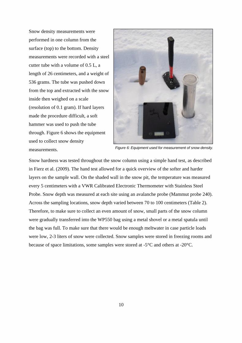
Snow density measurements were

performed in one column from the

surface (top) to the bottom. Density

measurements were recorded with a steel

cutter tube with a volume of 0.5 L, a

length of 26 centimeters, and a weight of

536 grams. The tube was pushed down

from the top and extracted with the snow

inside then weighed on a scale

(resolution of 0.1 gram). If hard layers

made the procedure difficult, a soft

hammer was used to push the tube

through. Figure 6 shows the equipment

used to collect snow density

measurements.

Snow hardness was tested throughout the snow column using a simple hand test, as described

in Fierz et al. (2009). The hand test allowed for a quick overview of the softer and harder

layers on the sample wall. On the shaded wall in the snow pit, the temperature was measured

every 5 centimeters with a VWR Calibrated Electronic Thermometer with Stainless Steel

Probe. Snow depth was measured at each site using an avalanche probe (Mammut probe 240).

Across the sampling locations, snow depth varied between 70 to 100 centimeters (Table 2).

Therefore, to make sure to collect an even amount of snow, small parts of the snow column

were gradually transferred into the WP550 bag using a metal shovel or a metal spatula until

the bag was full. To make sure that there would be enough meltwater in case particle loads

were low, 2-3 liters of snow were collected. Snow samples were stored in freezing rooms and

because of space limitations, some samples were stored at -5°C and others at -20°C.

Figure 6: Equipment used for measurement of snow density.

11

Table 2: Overview of snow depth at each sampling location.

STATION SNOW DEPTH

U1 70 cm

U2 90 cm

U3 90 cm

U4 70 cm

U5 100 cm

R1 70 cm

R2 80 cm

R3 70 cm

R4 70 cm

CONTROL 70 cm

12

2.5 Thawing of snow samples

Snow samples were taken out of the cold rooms at least 24 hours before the laboratory

procedure. During transport and thawing, the samples were handled with care so that no

mechanical stress would act on the bags. Samples that were kept at -20°C were double bagged

to preserve sample material due to higher prevalence of leaking.

2.6 Preparation of equipment for cleanroom

All handling of the thawed snow samples was done in the cleanroom located at the Institute

for Air Research (NILU), Tromsø. The equipment used for the filtration and staining

procedures had to be cleaned for all plastic particles. All glass and metal wares were washed,

covered in tinfoil, and burned at 500°C for 8 hours one day before use. To use the cleanroom

at NILU Tromsø, there was a strict chemical-free regime; this meant no use of cosmetic

products or soaps for 12 hours before entering the cleanroom. In the cleanroom, a synthetic

overall always had to be worn, in addition to boots and hood. The latter precautions were not

to prevent plastic contamination, but chemical contamination for other ongoing research.

During the sample processing, no gloves were worn to limit direct contact of synthetic

polymers.

2.7 Preparation of NR solution

NR solution was prepared in the cleanroom by dissolving a technical grade NR powder

(N3013, Sigma Aldrich) in 98% ethanol solution to obtain a concentration of 10 mg/L. The

NR solution was filtered through a Whatman 47mm GFF filter (WHA1825047, Sigma

Aldrich) to remove any plastic particles before transferring to the pre-burned glass container

and then covered with tin foil.

13

2.8 Filtration and staining of melted snow

The filtration equipment consisted of a 2 liter

Erlenmeyer flask, a filtration head with a connection

for the vacuum pump to be used with 47 mm filters,

and a 500 ml funnel (Figure 7). Three complete sets

were used simultaneously to process one location

(i.e., three sub-samples) in one day. In order to avoid

cross-contamination between subsamples, each

subsample was filtered with the same column. One

hundred ml of meltwater was filtered and pumped

dry before releasing the vacuum by disconnecting

the pump tube. The funnel wall was rinsed with

filtered water to remove any particles adhering to it.

With a glass pipette, ~2 ml NR solution was applied,

so that it covered the filter entirely with a thin layer

and was left to stain for five minutes. The pump was

connected to remove any excess NR in the filters.

The filter was rinsed with 50-100 ml of filtered

water to remove any remaining NR on the filter, as

this would show up during the visual analysis. The

funnel wall was thoroughly rinsed to make sure no

plastic particles remained on the equipment.

When all aliquots (3x5) of a location had been processed, the field blank WP550 bags were

filled with 500 ml of filtered water, shaken vigorously, and then processed following the same

procedure as described. To get an estimate of the possible contamination generated by the

laboratory process, 100 ml of filtered water was filtered and stained. After the filtering and

staining processes were completed, the filters could be removed from the cleanroom as

additional contamination would no longer be detected on the visual analysis.

Figure 7: Filtration setup used for filtering and staining of samples.

14

2.9 QA and QC sampling and sample treatment

To get an estimate of how many particles were added to the samples during handling in the

lab, as well as in the field, two different blank samples were taken throughout the sample

handling period: 1) field blank and 2) lab blank. For each sampling location, one open bag

was placed close to where the sampling was occurring. This field blank was then treated in the

same way as the regular samples. During the laboratory procedure, one filter was treated the

same way as the other samples but replacing melted snow with filtered water. However, as the

contamination in the lab also would be incorporated into the field blanks (handled indentically

to a sample in the lab), the laboratory blanks were used to assess the magnitude of

contamination during the handling in the lab. The lab blanks were not used to calculate a

method detection limit (MDL).

2.10 The method detection limit (MDL)

The method detection limit is an approach to identify method threshold limits. The MDL was

subtracted from each aliqout in the data. This removes the number of particles added by the

sample collection and processing. The MDL was calculated using Equation 1

𝑴𝑫𝑳 = 3 ∗ 𝑆𝑡𝑎𝑛𝑑𝑎𝑟𝑑 𝑑𝑒𝑣𝑖𝑎𝑡𝑖𝑜𝑛 (𝑏𝑙𝑎𝑛𝑘 𝑠𝑎𝑚𝑝𝑙𝑒𝑠) + 𝑚𝑒𝑎𝑛(𝑏𝑙𝑎𝑛𝑘𝑠 𝑠𝑎𝑚𝑝𝑙𝑒𝑠)

Equation 1: Equation to calculate the method detection limit (MDL).

The MDL was subsequently subtracted from the number of each aliquot. The MDL was, in

some cases, higher than the number of particles recorded for a subsample leading to negative

values for some subsamples. All values below the MDL were therefore set to zero.

15

2.11 Visual analysis

The filter with stained particles was placed under a

Leica M-50 with an MC190 camera attached to it. A 3D

printed filter holder containing eight blue LEDs and an

orange filter were attached to the stereomicroscope. The

LEDs would emit light waves at 470 nanometers

exciting the NR. The light emitted from the NR stained

particles would pass through the orange filter, while blue

light was filtered out (Figure 8). This allowed us to take

pictures of the filters with only the stained particles

visible. Pictures were taken at a resolution of 2596x1944

pixels (~5 megapixels) with a 0.63 times magnification.

The magnification of the stereomicroscope prevented

the opportunity of taking one picture of the complete

filter. Therefore, four pictures were taken through a grid

and later cropped down so that each picture included

one-fourth of a filter.

2.12 Image analysis

To standardize the way particles were counted and to decrease human error, the image

software ImageJ (version 1.52) was used. ImageJ allows to set a threshold based on the light

intensity; this was in our case set to 100 (out of 255) to exclude all dimly lit particles. In

addition to the threshold, only particles that measured more than 3 pixels were recorded. All

images were converted into black and white in Adobe Lightroom to use ImageJ for the count

of particles. Adobe Lightroom also allowed for removing light specks that appeared outside

the filter area. To count MPs from multiple images in sequence, a macro was written in

ImageJ that allowed counting all images in each folder containing images from each location.

For each location, 84 images were analyzed using ImageJ that provided both the number of

particles but also their largest diameter measured in pixels.

Figure 8: Schematic of stereomicroscope and light waves.

16

2.13 Comparing manual and automated counting

Randomly selected filters were counted manually and compared to the count obtained by

ImageJ. Counting was done using the multi-point tool in ImageJ, allowing for click counting

on the images taken through the Leica stereomicroscope.

2.14 Data frame and correction

The ImageJ macro (Appendix C) exported one excel file per picture with the number of

particles and the area for each picture; these were imported to R (Version 3.4.4) and combined

for each filter using the dplyr library.

2.14.1 Correcting for snow density

To be able to compare all stations, they had to be corrected for snow density. Snow density

was calculated using Equation 2.

𝑺𝒏𝒐𝒘 𝒅𝒆𝒏𝒔𝒊𝒕𝒚(𝒈. 𝑳−𝟏) =𝑤𝑒𝑖𝑔ℎ𝑡 𝑜𝑓 𝑡𝑢𝑏𝑒 𝑤𝑖𝑡ℎ 𝑠𝑛𝑜𝑤(𝑔) − 𝑤𝑒𝑖𝑔ℎ𝑡 𝑜𝑓 𝑒𝑚𝑝𝑡𝑦 𝑡𝑢𝑏𝑒(𝑔)

𝑣𝑜𝑙𝑢𝑚𝑒 𝑜𝑓 𝑡𝑢𝑏𝑒(𝐿)

Equation 2: calculation is done to get the snow density in grams per liter.

For each sampling location, three density samples were taken to get a more accurate snow

density measurement. These three samples were averaged.

The average density was then used to calculate a correction factor using Equation 3. The

density correction factor was calculated for each station.

𝑫𝒆𝒏𝒔𝒊𝒕𝒚 𝒄𝒐𝒓𝒓𝒆𝒄𝒕𝒊𝒐𝒏 𝒇𝒂𝒄𝒕𝒐𝒓 =𝑠𝑛𝑜𝑤 𝑚𝑙

𝑣𝑜𝑙𝑢𝑚𝑒 𝐿∗

𝑛 𝑝𝑎𝑟𝑡𝑖𝑐𝑙𝑒𝑠

100𝑚𝑙=

(𝑛 𝑝𝑎𝑟𝑡𝑖𝑐𝑙𝑒𝑠)

𝐿

Equation 3: Calculation of the multiplying factor to correct each station for snow density to get particles/L snow.

2.14.2 Calculating particle size

ImageJ offers several methods to measure the size of particles, where the most commonly

used is the area in pixels. Using a measurement function called Feret's diameter, the longest

diameter could be measured. The value for diameter was given in pixels and transformed into

micrometer using the software LAS EZ (Leica microsystems) while taking the magnification

into account. We calculated the length of one pixel to be 11.47µm at the used magnification.

17

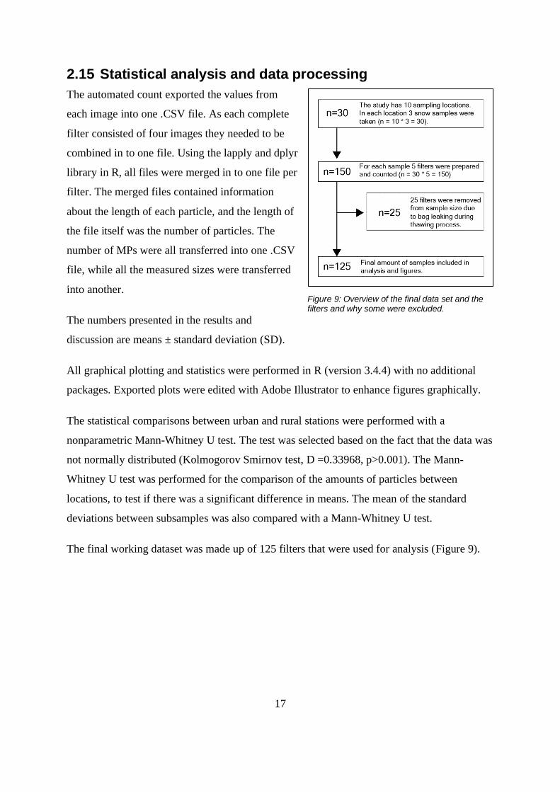
2.15 Statistical analysis and data processing

The automated count exported the values from

each image into one .CSV file. As each complete

filter consisted of four images they needed to be

combined in to one file. Using the lapply and dplyr

library in R, all files were merged in to one file per

filter. The merged files contained information

about the length of each particle, and the length of

the file itself was the number of particles. The

number of MPs were all transferred into one .CSV

file, while all the measured sizes were transferred

into another.

The numbers presented in the results and

discussion are means ± standard deviation (SD).

All graphical plotting and statistics were performed in R (version 3.4.4) with no additional

packages. Exported plots were edited with Adobe Illustrator to enhance figures graphically.

The statistical comparisons between urban and rural stations were performed with a

nonparametric Mann-Whitney U test. The test was selected based on the fact that the data was

not normally distributed (Kolmogorov Smirnov test, D =0.33968, p>0.001). The Mann-

Whitney U test was performed for the comparison of the amounts of particles between

locations, to test if there was a significant difference in means. The mean of the standard

deviations between subsamples was also compared with a Mann-Whitney U test.

The final working dataset was made up of 125 filters that were used for analysis (Figure 9).

Figure 9: Overview of the final data set and the filters and why some were excluded.

18

3 Development of protocol

The main aim of this thesis was to develop and test a method to sample, identify, and quantify

MPs in snow. For this purpose, a protocol was established describing each step from sample

collection, recording, and measuring essential parameters to QA, laboratory process,

analyzation, and quantification. None of the techniques used in the protocol are new, but

rather a collection of tested methods combined. The protocol serves as an effort to providing

standardized methods, with an emphasis that it could be easily adapted to other environmental

media and easy to reproduce. The protocol is attached in Appendix B.

3.1 Snow sampling

Our snow sampling protocol was based on (Gallet et al., 2018), with many elements

simplified or removed. Following personal advice by J-C Gallet the snow physical properties

recorded were density, depth, hardness, and temperature. All tools to record the listed

parameters were available to purchase within a short time, except for a snow density tool. J-C

Gallet provided a cutter tube with a known volume and weight for density measurements.

Following an assumption that there would be low amounts of microplastics in the snow, a

large sample container would be required. In (Gallet et al., 2018), a WP550 bag was used to

collect snow samples for environmental carbon; as this was light and robust, it was ideally

suited to our purpose. The drawback with WP550 bag is that it was made of high-density

polyethylene, which could be a potential contamination source that had to be accounted for.

Most equipment described in (Gallet et al., 2018) did not contain any or low amount of plastic

parts. The foldable plastic ruler described in the protocol was replaced by an avalanche probe

(Mammut probe 240).

3.2 QA and QC in the field

The most critical QA measure in the field was the field blank samples. The field blanks

provide an estimate on how much plastic contamination is due to the sampling process (i.e.,

particles from the container, handling, or the equipment used in sampling). Also, to assess

potential local contamination sources, each site was photographed, and any proximity to

plastic sources was reported. The blank samples are used to calculate an MDL which is

subtracted from the number of particles, ensuring that MPs present in the environment are

counted.

19

3.3 Storage and handling of snow samples

Since samples were collected and treated months apart, they had to be stored. Most samples

were stored in a cold room (-5°C), but due to space limitations, some samples were stored in a

freezer (-20°C). Samples stored in the freezer tended to leak when thawed, most likely due to

the formation of hard ice crystals perforating the sampling containers. Before being processed

and stained, all samples were thawed at room temperature for 24 hours. While thawing,

sample containers were placed in buckets to prevent them from tipping over and spilling.

Since contamination from the air could be an issue, all samples were kept closed during

transport and thawing. Based on our experience from the different storage temperatures, we

advise to store samples in a cold room at -5°C and to thaw samples with care.

3.4 Solvent and Nile red concentration

When reviewing the literature, different solvents and concentrations were reported (Erni-

Cassola et al., 2017; Maes et al., 2017; Shim et al., 2016). The most suitable solvent was

ethanol, whose use is associated with lower health risks. The concentration that was tested

and finally used was 10 mg/L. Although lower concentrations of NR have been reported as

successful, a cautionary approach was taken, and a slightly higher concentration of NR used.

3.5 Stereomicroscope modification

NR needs light waves between 450-510 nm to become fluorescent; this corresponds to the

blue to the green light spectrum. Most stereomicroscopes are not provided with an option with

light exclusively in that spectrum. To make a cost-effective option that did not require any

specialized orders, a microscope attachment was made with eight blue LEDs. The LEDs were

wired in parallel with a 33 Ω resistor each attached so they would not burn out. Using a USB

cable, they could be attached to a 5 V power source (Appendix Figure D1). To see the emitted

light from the NR, all the blue light needed to be filtered out. A deep orange filter film

(Eurolite, 158 deep orange) intended for theatre lights was used to filter out all the light

except for orange. Two layers of the filter film were needed to remove all blue light. The first

experimental stereomicroscope attachment was made entirely out of cardboard and hot glue; a

later 3D printed design was made by Jan Are Jacobsen at Norwegian Polar Institute. The 3D

printed version is available and attaches to all stereomicroscope with a Leica M-series 1.0x

Plan Objective. In addition, it is crucial to consider the background on which the filter will be

20

photographed. Black backgrounds worked best as they reduced light reflection and scattering,

reducing image noise.

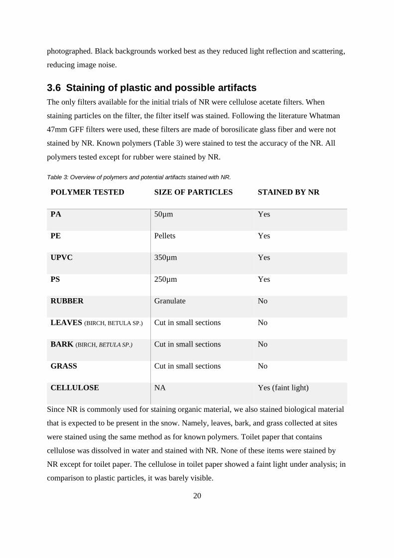
3.6 Staining of plastic and possible artifacts

The only filters available for the initial trials of NR were cellulose acetate filters. When

staining particles on the filter, the filter itself was stained. Following the literature Whatman

47mm GFF filters were used, these filters are made of borosilicate glass fiber and were not

stained by NR. Known polymers (Table 3) were stained to test the accuracy of the NR. All

polymers tested except for rubber were stained by NR.

Table 3: Overview of polymers and potential artifacts stained with NR.

POLYMER TESTED SIZE OF PARTICLES STAINED BY NR

PA 50µm Yes

PE Pellets Yes

UPVC 350µm Yes

PS 250µm Yes

RUBBER Granulate No

LEAVES (BIRCH, BETULA SP.) Cut in small sections No

BARK (BIRCH, BETULA SP.) Cut in small sections No

GRASS Cut in small sections No

CELLULOSE NA Yes (faint light)

Since NR is commonly used for staining organic material, we also stained biological material

that is expected to be present in the snow. Namely, leaves, bark, and grass collected at sites

were stained using the same method as for known polymers. Toilet paper that contains

cellulose was dissolved in water and stained with NR. None of these items were stained by

NR except for toilet paper. The cellulose in toilet paper showed a faint light under analysis; in

comparison to plastic particles, it was barely visible.

21

3.7 Establishing aliquot volume based on NR trials

One sample of ~5 L snow melted into 2-3 L of meltwater depending on density. Filtering the

whole sample would have led to an overload of particles on the filter. We also assumed that

the plastic particles within the sample were not uniformly distributed and that there should be

high variability between aliquots. Therefore, we processed, stained, and analyzed aliquots of

50, 100, 150, 200, 300, and 500 ml. Based on the number and layering of particles, 100 ml

aliquots were selected. Following the assumption of high variability within the samples due to

low homogeneity, we decided to analyze five aliquots of 100 ml from each subsample.

3.8 Filtration and staining of samples

Each of the three subsamples in a sample were processed using a different filtration set to

avoid cross-contamination between subsamples. The walls of the funnels were rinsed with

filtered tap water (pore size: 0.7 µm) to make sure all particles were washed down on the

filter. The most convenient and efficient way to stain the samples was to leave the filter in the

filtration setup and add the Nile Red solution onto the filter. This limited the handling of

filters. During initial trials of staining with NR, we found out that the vacuum pump had to be

disconnected when adding NR in order not to get sucked through the filter but remain on the

filter. The NR solution was left on the filter for 5 minutes to stain. The vacuum pump was

then reconnected, and the solution and filter were washed with prefiltered tap water to remove

any leftover NR. After the samples were filtered, stained, and rinsed, they could safely be

taken out of the cleanroom as they needed to be analyzed in a dark room.

3.9 QA and QC in the laboratory

Our method was performed in a cleanroom (NILU, Tromsø) to ensure minimal contamination

during the laboratory procedure. Most parts of the filtration equipment were made of glass or

metal. The major plastic equipment used in the laboratory procedure was the vacuum pump

and hose, but neither of them was in direct contact with the samples. The equipment and

filters were burned at 500°C for 8 hours before use to remove any residual microplastic

particles on it. Smaller equipment was packed in tin foil and openings of glass equipment

covered with tin foil. Procedural blanks, to estimate the plastic contribution from the

laboratory process, were obtained by processing filtered water in the same way as snow

samples using a clean filtration set.

22

3.10 Counting of microplastics

In order to capture the whole filter

with the microscope camera, we

took four images using a grid drawn

on a glass petri dish placed on top of

the filter (Figure 10). Each image

was cropped down to each quadrant

so that no part of the filter

overlapped. When examining the

test samples, it appeared that the

manual count of particles was time-

consuming since each filter displayed up to hundreds of particles. As an alternative, we

explored ways of automatic counting. We first created a script in R using the EBImage

library. The EBImage library was initially intended for the counting of nuclei in cells; it was

unpractical to adapt this method for counting microplastic particles. (Erni-Cassola et al.,

2017) reported the use of the software ImageJ which proved to be a better tool for counting

plastic particles. We, therefore, wrote a macro in ImageJ (using basic JavaScript) that allowed

not only the count of particles but also produced output information about the individual

particles such as their longest diameter and area in pixels. Using the software supplied with

the Stereomicroscope (Leica Application Suit X, Leica microsystems), the length of one pixel

in µm at the used magnification could be calculated. The combination of microscope

photography and the software ImageJ enabled the count of particles and measurement of their

sizes.

Thirty randomly selected filters were counted both manually and automated, to validate the

automated count. The manual count assured that the count from ImageJ did not overestimate

the number of plastic particles and could, therefore, be used for counting of MPs.

Figure 10: Schematic of how filters were photographed in quarters with the use of a lined petri dish.

23

4 Results

4.1 The occurrence of MP particles

The MDL calculated was 184 particles 100 ml-1; it was subtracted from each aliquot. It was

ensuring that the number of particles reported did not include contamination from the

sampling and/or laboratory procedure. The mean number of particles in the urban samples

was 681 ± 375 particles L-1 of snow, while the mean in the rural sites was 439 ± 286 particles

L-1 of snow. The number of particles was significantly different between urban and rural

locations (Mann Whitney U-test, U-value=2227, P<0.0001), being twice as high in the urban

areas compared to the rural areas (Figure 11).

Figure 11: Boxplot over the number of particles L-1 snow in all the urban locations (red) and all rural locations (green).

24

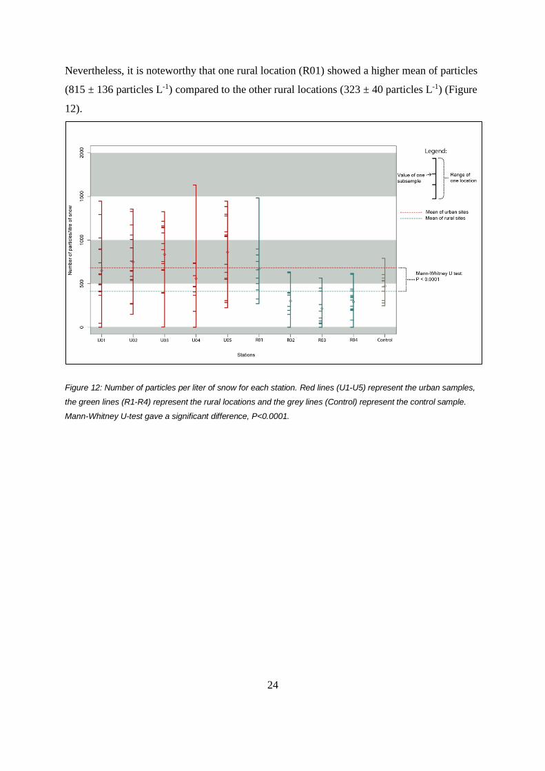
Nevertheless, it is noteworthy that one rural location (R01) showed a higher mean of particles

(815 ± 136 particles L-1) compared to the other rural locations (323 ± 40 particles L-1) (Figure

12).

Figure 12: Number of particles per liter of snow for each station. Red lines (U1-U5) represent the urban samples,

the green lines (R1-R4) represent the rural locations and the grey lines (Control) represent the control sample.

Mann-Whitney U-test gave a significant difference, P<0.0001.

25

The standard deviation for the urban stations was significantly higher than the standard

deviation for the rural stations (Figure 13). The average standard deviation was 25% higher

for urban stations compared to rural stations (375 vs. 286, respectively). The lowest variation

was in the control sample, indicating that the sample was more homogenous at the control site

than at any of the other sites. The standard deviation was 55% of mean number MPs in urban

locations, while in the rural stations, it was 65% of mean number MPs.

Figure 13: Bar plot of the standard deviation for each sampling location. Blue-green bars represent the urban locations; red represents rural locations; grey represents the control location. The red horizontal line represents the mean of the standard deviation in the urban locations, while the blue-green shows the mean of the standard deviation for the rural stations.

26

4.2 The difference in MP sizes between urban and rural sampling sites

The combination of the 0.63 times magnification and the 5-megapixel camera resolution, the

smallest length that could be recorded, was 22 µm in diameter. The longest length of particle

found in this study was 7983µm.

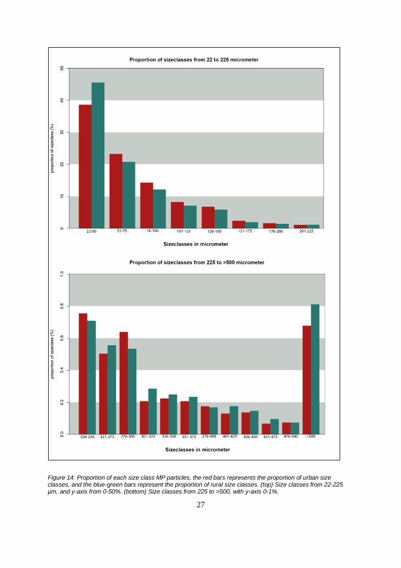
For both urban and rural stations, the most abundant MP particles were smaller than 200 μm

in diameter (Figure 14). The distribution of the smaller sizes differed when comparing urban

to rural areas. The rural stations had a higher proportion of the smallest size class (22-50 µm)

(45.5% vs. 38.6%); for all classes up to 200 µm, the urban stations had a slightly higher

proportion of MPs ranging from 2.5 % to a 0.2% difference. Overall, the mean of the urban

stations was 82.34 µm compared to 79.27µm for the rural stations (Mann Whitney U test, W=

20977000, p>0.0001) for all particles. MPs were grouped into size classes starting from 22-

500 µm or more; the grouping was in 25 µm increments; the only exceptions were the

smallest and largest size class. The rural stations had a higher proportion of the total amount

in the smallest size class.

27

Figure 14: Proportion of each size class MP particles, the red bars represents the proportion of urban size classes, and the blue-green bars represent the proportion of rural size classes. (top) Size classes from 22-225 µm, and y-axis from 0-50%. (bottom) Size classes from 225 to >500, with y-axis 0-1%.

28

4.3 Viability of the method

4.3.1 Field blanks and MDL

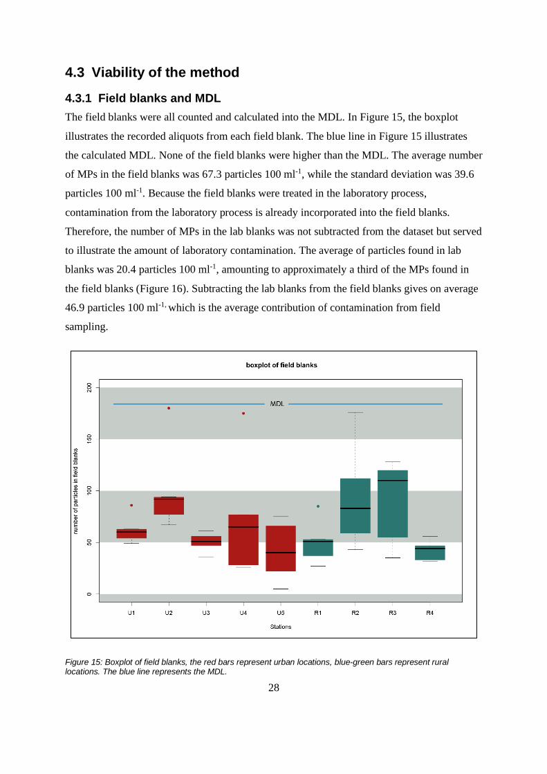
The field blanks were all counted and calculated into the MDL. In Figure 15, the boxplot

illustrates the recorded aliquots from each field blank. The blue line in Figure 15 illustrates

the calculated MDL. None of the field blanks were higher than the MDL. The average number

of MPs in the field blanks was 67.3 particles 100 ml-1, while the standard deviation was 39.6

particles 100 ml-1. Because the field blanks were treated in the laboratory process,

contamination from the laboratory process is already incorporated into the field blanks.

Therefore, the number of MPs in the lab blanks was not subtracted from the dataset but served

to illustrate the amount of laboratory contamination. The average of particles found in lab

blanks was 20.4 particles 100 ml-1, amounting to approximately a third of the MPs found in

the field blanks (Figure 16). Subtracting the lab blanks from the field blanks gives on average

46.9 particles 100 ml-1, which is the average contribution of contamination from field

sampling.

Figure 15: Boxplot of field blanks, the red bars represent urban locations, blue-green bars represent rural locations. The blue line represents the MDL.

29

Figure 16: Boxplot comparing the number of counted MPs in field blanks and lab blanks. The green box is for the field blanks, the yellow box is for the lab blanks.

4.3.2 Comparing manual count to automatic count

For all samples, the manual count was significantly higher than the automatic count (Mann

Whitney U test, W= 734.5, P<0.0001) (Figure 17) with a mean of 187 particles for the manual

count vs. 87 particles for the automatic count.

Figure 17: Comparison between manually counted and automatically counted particles in the same pictures.

30

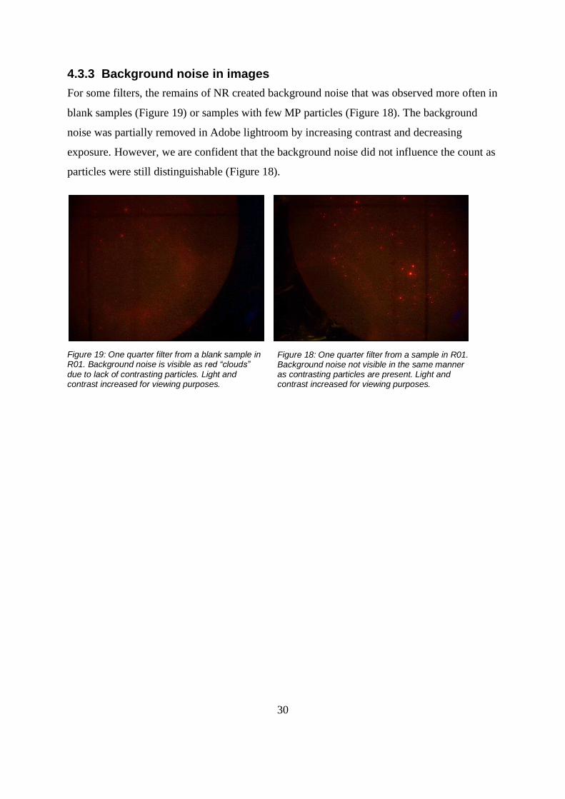
4.3.3 Background noise in images

For some filters, the remains of NR created background noise that was observed more often in

blank samples (Figure 19) or samples with few MP particles (Figure 18). The background

noise was partially removed in Adobe lightroom by increasing contrast and decreasing

exposure. However, we are confident that the background noise did not influence the count as

particles were still distinguishable (Figure 18).

Figure 19: One quarter filter from a blank sample in R01. Background noise is visible as red “clouds” due to lack of contrasting particles. Light and contrast increased for viewing purposes.

Figure 18: One quarter filter from a sample in R01. Background noise not visible in the same manner as contrasting particles are present. Light and contrast increased for viewing purposes.

31

5 Discussion

In recent years, MPs have been found in most natural media explored, highlighting the

importance of monitoring its presence. Confirming the presence of MPs in snow is essential to

understand alternative transport mechanisms across landmasses and from land to the ocean.

MP has been detected in snow before using different methodologies. The first study on snow

by Bergmann et al. (2019) showed the presence of plastic polymers in snow from the high

Arctic and central Europe using FTIR. The presence of MPs in snow from the Swiss Alps

used mass spectrometry for MP detection (Materić et al., 2020). Based on the limited number

of studies available and the lack of a harmonized sampling- and MP determination protocol,

snow as wet deposition acting as a vector for MP transport is still a relatively unexplored area

of research.

In this thesis, we developed a method using acknowledged snow sampling techniques and the

lipophilic staining chemical NR to identify and quantify microplastics. The method was tested

by trials with NR on a range of plastic polymers and exclusion of organic material (3.6),

followed by optimizing all sample handling steps from sampling in the field (3.1), storage

(3.3), sample treatment for MP enrichment (3.7, 3.8) and MP determination (3.6, 3.10). Also,

we developed a strict QA/QC protocol to ensure the minimization of contamination risk (3.2,

3.9).

The method was thereafter used to compare the occurrence of MPs in low-Arctic snow

collected in rural and urban locations. We sampled 10 locations consisting of three

subsamples per site, from which five aliquots were taken. With the optimized method, we

could process one location per day (15 aliquots from subsamples, five aliquots from the field

blank, and one aliquot from lab blank). The developed particle counting method can analyze

~50 filters per hour. The strict QA and QC regime that we developed reduced the

contamination risk by particles during the complete sample handling process to a mean of 46

particles 100 ml-1 from field samples and 21 particles 100 ml-1 from the laboratory process.

Resulting in a fieldblank of 184 particles 100 ml-1.

32

5.1 Method adaptation

5.1.1 Internal suitability of NR staining

The successful staining of known plastic polymer types by NR proved its efficacy to stain

plastic particles at concentrations of 10 mg L-1. Rubber from car tires did not react with NR.

Rubber from car tires are in a major source of MPs to the environment (Kole et al., 2017), and

therefore represents a drawback on the use of NR to stain environmental samples. Another

drawback is that NR also stains cellulose that could potentially be present in the snow that is

close to vegetation. To exclude some possible naturally occurring substances, grass, leaves,

and bark were stained with NR, but they did not cause any fluorescence. There are

possibilities to remove organic material from a sample with acid digestion (Claessens et al.,

2013), alkaline digestion (Dehaut et al., 2016), or enzymatic degradation (Löder et al., 2017).

As we did not expect NR to stain the organic material that was potentially present in the snow

sampled, we did not treat our samples. Additionally, sample treatment has the possibility to

damage plastic polymers. Ryan et al. (2019)found that acid digestion was not suitable for

isolation of MPs, alkaline digestion was more suited, however there were still uncertainties

associated with its use. Enzymatic digestion is more appropriate and would be our

recommendation if treatment of samples were to be done. It is time consuming and more

expensive, but the safest approach to not damage MP during an MP isolation step (Löder et

al., 2017; Ryan et al., 2019).

The goal of the sampling approach was to acquire enough samples for analysis. The number

of sites sampled for the study was 10. Two additional locations (not included in the study)

were used to develop and refine the NR staining and test different aliquot volumes. An aliquot

volume of 100 ml was decided upon, and five aliquots per subsample filtered to account for

high intra-subsample variation. The filtration was a standard filtration method with glass

equipment, glass fiber filters, and a vacuum pump. An automated counting method was

developed with the use of a JavaScript macro in ImageJ, that allowed for fast and reliable

counting of images. QA and QC were implemented by reducing the amount of plastic on

equipment used in the field sampling and laboratory process and by taking blank samples at

every step of the process to gain information about the contamination in sampling and sample

handling.

33

5.1.2 Determination of the MP count

The MDL calculated from the field blank samples was 184 particles 100 ml-1. In order to

maximize our confidence in the automated count of MP, the threshold of the particle count

was set to 100 (out of 255) light intensity, effectively removing all pixels that are dark from

the particle count. As background noise still could present as an issue, only MP that consisted

of three or more pixels were counted. The three pixels do not need to be connected in a

straight line to be counted, meaning that the lowest diameter measured was two pixels.

Although the protocol does not allow the identification of size classes below 22 µm, it

remains a good tool to identify differences in MP concentrations above that limit. Counting

visually introduces human bias to the count. Comparing the manual count to the automatic

count, it was apparent that ImageJ consistently counted lower numbers (Figure 17). The

significantly lower count was because ImageJ had strict counting criteria, while the human

eye cannot differentiate as accurately. The counting and recording of sizes with ImageJ

provided consistent results, making them comparable. The thresholds set in ImageJ were

strict; this ensured that the ImageJ count was a conservative number. As the threshold applied

was the same for all samples, the counted numbers were comparable between the sites. Lenz

et al. (2015) also found a discrepancy between the manual and automatic count, however

more related to if a particles are plastic polymers or not. In our study background noise could

be counted as MPs and the threshold distinguishes between particles and background noise.

5.1.3 Comparability with other MP detection methods

The staining of plastic particles with NR has been used successfully in several studies (Erni-

Cassola et al., 2017; Maes et al., 2017; Shim et al., 2016). The repeated use of NR in studies

on microplastic confirms its suitability. However, some flaws with inadvertent staining of

particles that are not plastic have been uncovered. NR staining of microplastic particles has

been validated for environmental media by two studies. Maes et al. (2017) validated the use of

NR to stain plastic, by both demonstrating that NR did not stain other matter present in their

samples and by validating their results with FTIR spectroscopy. Erni-Cassola et al. (2017)

validated the identification of MPs with Raman spectroscopy. Both studies concluded that the

NR staining of MPs is a quick and effective method to identify and count MP particles in

environmental media but cautioned about possible false positives. Maes et al. (2017)

uncovered that NR potentially could be used to differentiate between polymers but limited to

polarity differences in plastic polymers.

34

5.2 Application of the method for the determination of MPs in snow

After subtracting the MDL, 95.4% of the aliquots were above the limit of detection. After

correcting the number of MP particles for snow density, the numbers of MPs ranged from 0

to1802 particles L-1 of snow. The standard deviations for both the urban and rural locations

were higher than 50% of the number of particles observed. The largest MP particle recorded

was from an urban station and measured 7983 µm, while the smallest particles recorded were

at the lowest resolution of the method, i.e. 22 µm.

5.2.1 Amount of microplastics in rural and urban areas

In this study, we found a significantly higher number of MP particles in the snow of urban

areas compared to rural areas. We found a mean of 681±375 particles L-1 in urban samples

and a mean of 439±286 particles L-1 in rural samples. The standard deviation was higher in

rural samples (375) than in urban samples (286) (Figure 13). The proportion of the standard

deviation compared to the mean number of MPs was lower in the urban sites (55%) than in

rural sites (65%). The high difference between subsamples within locations show that

microplastic particles in snow has a heterogenic distribution. With a heterogenic distribution it

is important to make sure the sample volume is sufficient enough to compensate for the MP

distribution within snow. Also, the high standard deviation observed in this study highlights

the importance of having a sufficient number of subsamples at all sampling locations. These

results suggest that both the urban and rural areas are strongly influenced by local pollution.

Although the rural sites had fewer local pollution sites close by (~40km to Tromsø city), the

lower number of MPs in the rural site suggests that they can have traveled with atmospheric

transport. As none of the rural sampling sites were further than 40 km away from the city, it

cannot yet be classified as LRT. Indeed, evidence of LRT of MPs requires snow samples from

remote sites like in the high Arctic or sampling a gradient away from a source site until stable

background levels can be reached.

Our findings are similar to a study performed in Paris, France, where suburban areas showed a

significantly smaller amount of MP particles in the rain and dry deposition compared to dense

urban areas (Dris et al., 2016). Dris et al. (2016) found that in the urban areas there was an

average atmospheric fallout of 110 ± 96 particles/m2/day, while in the suburban areas it was

53 ± 38 particles/m2/day. The authors suggested that there was a more substantial amount of

35

local pollution in the urban areas, causing a higher concentration of plastic particles in

atmospheric fallout (Dris et al., 2016).

Bergmann et al., (2019) recorded MP concentrations comparing high arctic locations to

locations in central Europe and reported a significantly higher number of particles for central

Europe. Their findings are presented in particles per liter of melted snow while ours are

presented in particles per liter of snow. For ease of comparison, we recalculated our numbers

presented in this section to partciles per liter of meltwater. The number of particles Bergmann

et al. (2019) found in the Arctic ranged from 0 to 14.4×103 particles L-1. In central Europe, the

number ranged from 0.19×103 to 154×103 particles L-1. We found on average of

2.27±0.14×103 particles L-1 in the urban locations and 1.24±0.15×10-3 particles L-1 in the rural

locations. The number of particles reported is difficult to compare, as the FTIR spectroscopy

used in Bergmann et al. (2019) had a higher resolution and could detect MPs down to 11 µm

while our smallest MP size detected was 22 µm.

Nevertheless, our results are within the same order of magnitude as Bergmann’s results,

confirming the applicability of our method. This is to be expected, as our locations are neither

in the high Arctic nor in central Europe. Our urban samples are most likely more influenced

by local pollution than those of Bergmann et al. (2019), and they do not span over such a

large geographical area. The number of data points in our study is, however, increasing the

confidence in our findings. The number of datapoints accounts for the variation between

subsamples and the variation between aliquots. The rigorous QA and QC have proved to be

vitally necessary as the contamination during every sample handling step can have a large

impact (Figure 15).

In general, snow density varies depending on several environmental conditions like wind,

temperature, and exposure to the sun. This most likely affects the concentrations of particles

found in the snow. For this reason, we highly recommend that snow density is measured as a

supporting variable and that the number of particles is corrected for this parameter.

Comparing the number of particles per liter of snow instead of per liter of meltwater accounts

for the varying snow densities recorded between locations. We also stress the importance of

having a sufficient number of subsamples to account for the heterogenic distribution of MP in

snow.

36

5.2.2 Size classes of MP particles in urban and rural stations

The MPs found in the urban locations had a significantly larger mean size than those found in

the rural locations. We predcited that the average size of MPs in rural locations would be

smaller. Although the difference in size was statistically significant, the difference was only

3.07 µm, which is not enough to fully support our assumption. Also, the smallest size class

represented the highest proportion in the rural areas (Figure 14), potentially responsible for

the observed difference in average size between areas, and caused by the higher potential of

smaller, lighter particles to travel farther by air than larger particles. For most other size

classes, urban areas exhibited the highest proportion. While Bergmann et al. (2019) did record

the sizes of MP particles, they did not compare the MP sizes between central Europe and the

Arctic. Bergmann et al. (2019) found MP particles ranging from 11 to 465 µm in length, and

fibers ranging from 65-14,314 µm in length. Their proportion of MP lengths followed a

similar power-law distribution as we found. Whether MPs found in the Arctic are

significantly smaller than in central Europe remains to be documented. Nevertheless, we

expect MP particles found in remote areas to be smaller and lighter than those found in more

densely populated areas.

5.3 Study conclusion

The main aim of the thesis was to establish a protocol for MPs in snow samples that is

inexpensive, robust, and easy to use. The study comparing the urban and rural locations in

Troms county was carried out in addition to prove the applicability and the ease of the

method. The results of our study are conservative and most likely not fully representative of

the real MP concentration in snow. However, they give an essential indication of the range in

particle numbers and sizes to expect. Experience gained during the trial was used to refine the

protocol. The protocol provides a method that can be used with commonly available

equipment, both for sampling and laboratory procedures. As the snow samples can be stored

in a cold room (-5°C), it is also possible to preserve samples over time. The most important

aspects are related to QA and QC, the use of a clean-room/ -chamber is not strictly necessary,

and if not available, the contamination must be estimated rigorously by having many blank

samples.

37

5.4 Perspective for future research and practice

To gain a holistic understanding of the potential LRT of MPs, the harmonization of methods

in MP research is essential. In this thesis, we developed a protocol that can be used anywhere

if standard laboratory equipment is available, without the need for expensive analytical

equipment and requiring specialized staff to operate. Making raw data of particle counting

available is also of importance as to compare studies and make inferences, notably as the

resolutions increase and sizes reported become smaller. If LRT of MPs is to be investigated, a

large-scale sampling effort must be performed, including several cities and remote areas,

while taking meteorological conditions into account. Fresh snow sampling would also be of

interest as it would create a more accurate picture of MPs present in the atmosphere at a given

time.

38

6 Conclusion

The method developed proved to work efficiently, as it was not arduous to apply for neither

the snow sampling nor the laboratory procedure. It should be considered as a tool in MP

research. The lack of specialized equipment makes the method available for use in the most

basic of research environments. The resolution of the method can be improved notably by

increasing either camera resolution or magnification. With the use of an electronically

controlled moving stage on the stereomicroscope, filters can be photographed in the same

manner. This would allow the increase of magnification, and we could theoretically measure

MPs down to 3 µm.

Even though the data from this study are not enough to support the theory of atmospheric

LRT of MPs, we could identify differences between urban and rural locations. This is

revealing that local pollution impacts the number of MPs in snow. The presence of MPs in

rural locations can be indicative of atmospheric transport. However, we still assume a

substantial part of the MPs to come from local terrestrial pollution.

39

References

Andrady, A. L. (2011). Microplastics in the marine environment. Marine Pollution Bulletin,

62(8), 1596–1605. https://doi.org/10.1016/j.marpolbul.2011.05.030

Barboza, L. G. A., Dick Vethaak, A., Lavorante, B. R. B. O., Lundebye, A.-K., &

Guilhermino, L. (2018). Marine microplastic debris: An emerging issue for food

security, food safety and human health. Marine Pollution Bulletin, 133, 336–348.

https://doi.org/10.1016/j.marpolbul.2018.05.047

Bergmann, M., Mützel, S., Primpke, S., Tekman, M. B., Trachsel, J., & Gerdts, G. (2019).

White and wonderful? Microplastics prevail in snow from the Alps to the Arctic. Science

Advances, 5(8), eaax1157. https://doi.org/10.1126/sciadv.aax1157

Boucher, J., & Friot, D. (2017). Primary microplastics in the oceans: A global evaluation of

sources. In Primary microplastics in the oceans: A global evaluation of sources. IUCN

International Union for Conservation of Nature.

https://doi.org/10.2305/IUCN.CH.2017.01.en

Browse, J., Carslaw, K. S., Arnold, S. R., Pringle, K., & Boucher, O. (2012). The scavenging

processes controlling the seasonal cycle in Arctic sulphate and black carbon aerosol.

Atmospheric Chemistry and Physics, 12(15), 6775–6798. https://doi.org/10.5194/acp-12-

6775-2012

Claessens, M., Van Cauwenberghe, L., Vandegehuchte, M. B., & Janssen, C. R. (2013). New

techniques for the detection of microplastics in sediments and field collected organisms.

Marine Pollution Bulletin, 70(1–2), 227–233.


Cózar, A., Martí, E., Duarte, C. M., García-de-Lomas, J., van Sebille, E., Ballatore, T. J.,

Eguíluz, V. M., González-Gordillo, J. I., Pedrotti, M. L., Echevarría, F., Troublè, R., &

Irigoien, X. (2017). The Arctic Ocean as a dead end for floating plastics in the North

Atlantic branch of the Thermohaline Circulation. Science Advances, 3(4), e1600582.

https://doi.org/10.1126/sciadv.1600582

Dehaut, A., Cassone, A.-L., Frère, L., Hermabessiere, L., Himber, C., Rinnert, E., Rivière, G.,

Lambert, C., Soudant, P., Huvet, A., Duflos, G., & Paul-Pont, I. (2016). Microplastics in

seafood: Benchmark protocol for their extraction and characterization. Environmental

Pollution, 215, 223–233. https://doi.org/10.1016/j.envpol.2016.05.018

Dris, R., Gasperi, J., Saad, M., Mirande, C., & Tassin, B. (2016). Synthetic fibers in

atmospheric fallout: A source of microplastics in the environment? Marine Pollution

Bulletin, 104(1–2), 290–293. https://doi.org/10.1016/j.marpolbul.2016.01.006

Eriksen, M., Maximenko, N., Thiel, M., Cummins, A., Lattin, G., Wilson, S., Hafner, J.,

Zellers, A., & Rifman, S. (2013). Plastic pollution in the South Pacific subtropical gyre.

Marine Pollution Bulletin, 68(1–2), 71–76.


Erni-Cassola, G., Gibson, M. I., Thompson, R. C., & Christie-Oleza, J. A. (2017). Lost, but

Found with Nile Red: A Novel Method for Detecting and Quantifying Small

Microplastics (1 mm to 20 μm) in Environmental Samples. Environmental Science &

Technology, 51(23), 13641–13648. https://doi.org/10.1021/acs.est.7b04512

Eunomia. (2016). Eunomia (2016) Plastics in the Marine Environment (Issue June).

www.eunomia.co.uk

40

Fierz, C., Armstrong, R., Durand, Y., & Etchevers, P. (2009). The International

Classificationi for Seasonal Snow on the Ground: Vol. IHP-VII Te.

https://unesdoc.unesco.org/ark:/48223/pf0000186462

Gallet, J. C., Bjorkman, M. P., Larose, C., Luks, B., Martma, T., & Zdanowicz, C. (2018).

Protocols and recommendations for the measurement of snow physical properties, and

sampling of snow for black carbon, water isotopes, major ions and microorganisms.

http://hdl.handle.net/11250/2486183

Geyer, R., Jambeck, J. R., & Law, K. L. (2017). Production, use, and fate of all plastics ever

made. Science Advances, 3(7), e1700782. https://doi.org/10.1126/sciadv.1700782

Hall, N. M., Berry, K. L. E., Rintoul, L., & Hoogenboom, M. O. (2015). Microplastic

ingestion by scleractinian corals. Marine Biology, 162(3), 725–732.

https://doi.org/10.1007/s00227-015-2619-7

Hepsø, M. O., Salaberria, I., Schmid, R., & Booth, A. M. (2018). Experimental weathering of

microplastics under simulated environmental conditions. In Master Thesis. The

Norwegian University of Science and Technology.

Kanhai, L. D. K., Gardfeldt, K., Krumpen, T., Thompson, R. C., & O’Connor, I. (2020).

Microplastics in sea ice and seawater beneath ice floes from the Arctic Ocean. Scientific

Reports, 10(1), 5004. https://doi.org/10.1038/s41598-020-61948-6

Keller, A. S., Jimenez-Martinez, J., & Mitrano, D. M. (2020). Transport of Nano- and

Microplastic through Unsaturated Porous Media from Sewage Sludge Application.

Environmental Science & Technology, 54(2), 911–920.

https://doi.org/10.1021/acs.est.9b06483

Kole, P. J., Löhr, A. J., Van Belleghem, F., & Ragas, A. (2017). Wear and Tear of Tyres: A

Stealthy Source of Microplastics in the Environment. International Journal of

Environmental Research and Public Health, 14(10), 1265.

https://doi.org/10.3390/ijerph14101265

Lenz, R., Enders, K., Stedmon, C. A., Mackenzie, D. M. A., & Nielsen, T. G. (2015). A

critical assessment of visual identification of marine microplastic using Raman

spectroscopy for analysis improvement. Marine Pollution Bulletin, 100(1), 82–91.


Löder, M. G. J., Imhof, H. K., Ladehoff, M., Löschel, L. A., Lorenz, C., Mintenig, S., Piehl,

S., Primpke, S., Schrank, I., Laforsch, C., & Gerdts, G. (2017). Enzymatic Purification of

Microplastics in Environmental Samples. Environmental Science & Technology, 51(24),

14283–14292. https://doi.org/10.1021/acs.est.7b03055

Maes, T., Jessop, R., Wellner, N., Haupt, K., & Mayes, A. G. (2017). A rapid-screening

approach to detect and quantify microplastics based on fluorescent tagging with Nile

Red. Scientific Reports, 7(1), 44501. https://doi.org/10.1038/srep44501

Materić, D., Kasper-Giebl, A., Kau, D., Anten, M., Greilinger, M., Ludewig, E., van Sebille,

E., Röckmann, T., & Holzinger, R. (2020). Micro- and Nanoplastics in Alpine Snow: A

New Method for Chemical Identification and (Semi)Quantification in the Nanogram

Range. Environmental Science & Technology, 54(4), 2353–2359.

https://doi.org/10.1021/acs.est.9b07540

Maximenko, N., Hafner, J., & Niiler, P. (2012). Pathways of marine debris derived from

trajectories of Lagrangian drifters. Marine Pollution Bulletin, 65(1–3), 51–62.


Neves, D., Sobral, P., Ferreira, J. L., & Pereira, T. (2015). Ingestion of microplastics by

commercial fish off the Portuguese coast. Marine Pollution Bulletin, 101(1), 119–126.


41

Obbard, R. W., Sadri, S., Wong, Y. Q., Khitun, A. A., Baker, I., & Thompson, R. C. (2014).

Global warming releases microplastic legacy frozen in Arctic Sea ice. Earth’s Future,

2(6), 315–320. https://doi.org/10.1002/2014EF000240

Rillig, M. C. (2012). Microplastic in Terrestrial Ecosystems and the Soil? Environmental

Science & Technology, 46(12), 6453–6454. https://doi.org/10.1021/es302011r

Ryan, P., Shim, W., Zhang, W., Mason, S., Galgani, F., Turra, A., Kershaw, P., Hong, S.,

Hassellöv, M., Lusher, A., Thiel, M., Eriksen, M., Takada, H., Tahir, A., Wilcox, C.,

Hardesty, B., & Uhrin, A. (2019). GESAMP 2019 Guidelines for the monitoring &

assessment of plastic litter in the ocean Reports & Studies 99 (editors Kershaw, P.J.,

Turra, A. and Galgani, F.).

Shim, W. J., Song, Y. K., Hong, S. H., & Jang, M. (2016). Identification and quantification of

microplastics using Nile Red staining. Marine Pollution Bulletin, 113(1–2), 469–476.


Sommer, F., Dietze, V., Baum, A., Sauer, J., Gilge, S., Maschowski, C., & Gieré, R. (2018).

Tire Abrasion as a Major Source of Microplastics in the Environment. Aerosol and Air

Quality Research, 18(8), 2014–2028. https://doi.org/10.4209/aaqr.2018.03.0099

Sundt, P., Schulze, P.-E., & Syversen, F. (2014). Sources of microplastic-pollution to the

marine environment m321. 86.

https://www.miljodirektoratet.no/globalassets/publikasjoner/M321/M321.pdf

Thomas, J. L., Polashenski, C. M., Soja, A. J., Marelle, L., Casey, K. A., Choi, H. D., Raut,

J.-C., Wiedinmyer, C., Emmons, L. K., Fast, J. D., Pelon, J., Law, K. S., Flanner, M. G.,

& Dibb, J. E. (2017). Quantifying black carbon deposition over the Greenland ice sheet

from forest fires in Canada. Geophysical Research Letters, 44(15), 7965–7974.

https://doi.org/10.1002/2017GL073701

Trevail, A. M., Gabrielsen, G. W., Kühn, S., & Van Franeker, J. A. (2015). Elevated levels of

ingested plastic in a high Arctic seabird, the northern fulmar (Fulmarus glacialis). Polar

Biology, 38(7), 975–981. https://doi.org/10.1007/s00300-015-1657-4

Yonkos, L. T., Friedel, E. A., Perez-Reyes, A. C., Ghosal, S., & Arthur, C. D. (2014).

Microplastics in Four Estuarine Rivers in the Chesapeake Bay, U.S.A. Environmental

Science & Technology, 48(24), 14195–14202. https://doi.org/10.1021/es5036317

I

Appendix A

A1 Raw data Table A 1: Table containing the raw number of particles per liter of snow. Aliqouts A1-A5 are from subsample A, Aliqouts B1-B5 are from subsample B and Aliqouts C1-C5 are from subsample C. U1-U5 are samples from urban locations, R1-R4 are samples from rural locations. C is the control sample.

ALIQUOT U1 U2 U3 U4 U5 R1 R2 R3 R4 C

A1 464 251 3 NA 1393 1802 634 688 438 NA

A2 382 136 351 NA 1456 327 643 507 107 NA

A3 342 698 657 NA 1053 606 398 549 0 NA

A4 385 506 360 NA 1304 393 197 227 0 NA

A5 455 597 1033 NA 1047 916 376 87 539 NA

B1 0 245 1030 518 726 NA NA 48 273 176

B2 42 591 976 1430 307 NA NA 59 784 294

B3 562 1247 1048 159 225 NA NA 129 258 501

B4 834 974 1096 355 552 NA NA 0 564 357

B5 571 537 1196 648 565 NA NA 318 453 261

C1 690 494 865 639 1285 519 404 NA 402 339

C2 837 1080 594 408 1104 683 242 NA 248 337

C3 1207 925 591 411 1066 798 149 NA 312 382

C4 1350 837 678 322 634 1007 0 NA 471 193

C5 956 1223 801 0 285 1091 0 NA 798 156

II

A2 Raw data of field blanks Table 4: From each location 5 aliqouts were taken from the fieldblank. U1-U5 are samples from urban locations, R1-R4 represent samples from rural locations.

ALIQUOT U1 U2 U3 U4 U5 R1 R2 R3 R4

1 60 180 56 77 75 53 176 101 44

2 54 94 51 28 66 51 83 128 47

3 49 92 36 26 22 27 112 120 33

4 63 67 47 175 40 37 43 55 32

5 86 77 61 65 5 85 59 35 56

III

Appendix B

Protocol for detection of microplastics in snow

Introduction

Microplastics in the snow is a new field in plastics research; this protocol is, therefore, a

contribution to standardizing methods. Contamination in plastics research is a widespread issue,

and the protocol will include blank samples at all stages of the sampling and analyzation

process.

Microplastic present in snow can have several origins, where local contamination and

atmospheric transport are suspected to be the main sources. Local contamination would

contribute to larger microplastics and macro plastics. Snow acts as a scavenger of particles

suspended in the air. If the wind transports microplastics, they should be found in the snow, and

these will probably range from small size microplastics to nano plastics.

The method of sampling is based on (Gallet et al., 2018), with some adaptations made to account

for the plastic contamination of the samples and explaining the process for determining if there

are microplastics in the sample.

QA and QC for field sampling

Avoiding and testing contamination

During the sampling procedure, there is a high chance of self-contamination. Most of the tools

used should not be made out of any plastic components. The problem is the container used for

the snow, whirl-pak 550 consisting of low-density polyethylene (LDPE), which possibly will

contaminate the sample. Excavate the snow pits using a shovel made of steel or a metal alloy

to avoid plastic contamination from the shovel. Clothes worn during the sampling could also

lead to possible contamination. Contamination by clothes will mostly be microfibers. Avoid

plastic contamination by wearing natural fibers (wool, cotton, etc.) to reduce the direct

contamination of the sample. Since plastic makes up almost all products we associate with daily,

there are many possible sources for contamination which makes investigation of microplastics

difficult.

IV

To see if there is any contamination during sampling or laboratory processing, there will have

to be several blank samples. When taking snow samples, an open bag will be placed on the side

of the excavation to catch any contamination when taking the snow samples.

Preparation for snow sampling

Metadata

1. Note GPS coordinates with the geoid reference system (ex. WGS84, NAD84).

2. Take photos of sampling sites and notation of possible local contaminants and distance

to them, most important roads, buildings, and other obstructions.

3. Take a photo of clothes worn during sampling or a notation of what material they

consisted of.

4. Estimate and note down the distance to local variations such as open ground, open water,

anything that could impact snowpack conditions.

5. Record meteorological conditions such as time since last snowfall, wind direction, cloud

cover, or direct sunlight.

Sampling equipment

Snow sampling does not require a large amount of specialized equipment. Dealing with

microplastic sampling does require a particular emphasis on limiting contamination. The

equipment has to be as plastic-free as possible to decrease contamination.

Shovels made of mainly aluminum or steel, and they need to be sturdy as this is one of the tools

that is most likely to break; bringing several will decrease the risk of sampling failure.

Snow saws can be useful to create clean edges and break harder layers.

Foldable ruler or avalanche probe with measurements to measure snow depth. Avalanche

probes are more useful than foldable rulers as they tend to break in cold and wet conditions. If

Avalanche probes are not available, bring several foldable rulers.

Thermometer with wit external probe to measure temperature within the snow layers.

Snow density tool can be acquired from snowmetrics (rip cutter) or a metal tube with known

weight and volume.

V

Weight scale to weigh snow in the snow density tool. The resolution of the scale varies

depending on the volume of the snow density tool. For 0.5 L of snow, a resolution of 1 gram is

enough.

Sampling containers for snow. Such as the whirl pak 550. Metal or glass containers are more

advantageous, but they are unpractical. Use an appropriate container to get an adequate amount

of snow and fits the practicalities of fieldwork.

Recommendations on digging snow pits

For high-quality samples, snow pits must be excavated with care following certain precautions

to limit contamination and correctly measure snow physical properties.

1. The orientation of the snowpit should be towards the sun, with the wall on which

sampling will take place being in the shade.

2. Snow extracted by creating the snow pits has to be disposed of downwind as far away

as possible to avoid snow drifting back into the pit.

3. Snow pits have to be large enough, so movement is not restricted, and there is space to

complete sampling without touching the walls.

4. On days with strong winds, it might be useful to create walls upwind of the snow pit to

shelter sampling from the wind. It is essential to not trample the area above the wall

where sampling is going to take place.

5. On glaciers and areas where the snow is older than one year, it is important to dig down

to the snow-firn-ice transition, if the pit is deeper than one metre, stairs or a ladder might

be of use.

VI

Sampling for snow

VII

Temperature

Measure the temperature at first because the walls quickly increase or decrease in temperature

when exposed to the surrounding environment (Gallet et al., 2018).

Take temperature measurements every 5 centimeters at the top 20 centimeters, and then one

measurement for each discrete layer with at least one measurement for every 10 centimeters.

Snow stratigraphy

Use a ruler to record the depth of each measurement and stratigraphy, 0 cm is always on the top

of the snowpit (0cm = surface of the snowpit). Snow hardness is the simplest of the snow

stratigraphic parameters to record, and it does not require any specialized equipment, only a

pen, and a knife. Insert objects from largest to smallest into the snow following table 1. Record

which objects successfully entered to estimate snow hardness throughout the column.

Term

Hand hardness test Ram² test (N) Symbol

Index Object Code Range Mean

Very soft 1 Fist F 0-50 20 /

Soft 2 4 fingers 4F 50-175 100 X

Medium 3 1 finger 1F 175-390 250 //

Hard 4 Pencil¹ P 390-715 500

Very Hard 5 Knife

blade

K 715-1200 1000

Ice 6 Ice I >1200 >1200 O

Table 1. Recommended hardness scale from (Fierz et al., 2009)

VIII

Snow density

Measure snow density for the whole snow column. The simplest way is to use a steel tube

with a known length and radius to calculate the volume. The larger the amount, the less the

margin of error, use a high-resolution scale if snow density tool is low volume.

The first step is to weigh the empty tube on the scale and noting down its weight that will be

subtracted later. Then insert the tube into the snow and block the lower end and weigh the

tube with the snow inside.

If there are hard or icy layers, a sturdy tube can be hammered to break through more robust

layers. If this is not possible, use a snow saw to cut out a piece, measure its dimensions and

weight to calculate its density.

After the weight of each layer is recorded using a simple equation for density calculation.

𝐷𝑒𝑛𝑠𝑖𝑡𝑦 (𝑔𝑟

𝑙) =

𝑠𝑛𝑜𝑤 𝑚𝑎𝑠𝑠 (𝑔𝑟)

𝑣𝑜𝑙𝑢𝑚𝑒 𝑜𝑓 𝑡𝑜𝑜𝑙 (𝑙)

Measuring snow density is an essential step as it will enable you to calculate the number of

microplastics or other particles per unit of volume.

Sampling for plastic particles

The suggested bag for sampling snow samples are the 5441 ml whirl-pak bags. The amount of

snow to be sampled has to be relatively high to assure a higher rate of microplastics per

sample as the expected levels in snow are low. The amount of meltwater from a given snow

sample is dependent on the density.

To make sure that you get a sample from the whole snow column transfer small amounts each

time to fill the bag up as much as possible with an even amount from each layer. At each site,

take three subsamples. When doing one of the samples open up a second sampling bag that

will be open during the whole procedure, this will be used as a blank sample to correct any

results for self-contamination.

It is important to stress the fact that the equipment used for snow samples have to be as

plastic-free as possible, and if there is any unnecessary plastic equipment nearby that this is

stored a couple of meters away downwind. If the samples are analyzed for polymer type, test

IX

the equipment so that those polymers can be taken into account as possible self-

contamination.

QA and QC for Laboratory procedures

Avoiding and testing for contamination

Laboratory processes can contribute a substantial input of microplastic particles, potentially

influencing results. There are two ways to counteract the contamination, blank samples, and

working on the sample in an environment with a low amount of plastic. Do blank samples either

way, and they should preferably account for all equipment used and represent the whole

laboratory procedure after opening the sample containers. Processing samples in a cleanroom

is advantageous if it is equipped with overpressure to keep particles out and a particle filter to

filter ingoing air. The use of a laminar flow cabinet can replace a clean room as long as the flow

is going out and not in.

Preparation of laboratory analysis filtration and staining equipment

• Glass pipettes

• Erlenmeyer flask

• 250ml beakers

• 500ml funnel

• Clamps

• Compressor base

• 47mm GFF filters

• Metal tweezers

• Tinfoil

• Vacuum pump

• Nile red

• Ethanol

• Brown glass jars

All filters and equipment made out of glass or metal should be burned before use to rid it

of any plastic residue.

Melting of snow

Snow samples should be thawed at room temperature without external heat applied, to protect

the sampling container and limit the number of particles coming off the bags. For samples

X

stored below freezing, there is a risk of snow having sharp edges that puncture the bags. To

ensure that the bags do not leak during melting, pack the sample in a second bag.

Nile red solution

Mix 3 mg, technical grade Nile red with 300 ml ethanol to create a 0.1 mg/ml solution. When

the Nile red is diluted, filter the solution with a GFF filter to remove any plastic particles.

Laboratory analysis of snow samples

Filtration and staining

Decide the desired sub-sample size and retrieve it from the melted samples. Make sure that

the subsample size does not contain too many particles to avoid stacking. Trial runs should be

performed for new samples to decide what volume works the best.

Samples are filtered through GFF filters in the filtration setup with a compressor pump. After

releasing a vacuum, use a glass pipette for bathing the filter in a layer of Nile red solution and

letting it stain for 5 minutes. Turn on the compressor pump to remove any excess Nile red

solution and then rinse the filter to remove any leftover color on the filter. Pack filters in

aluminum foil to prevent exposure to plastic particles and light.

Visual analysis

The plastic particles stained with Nile red will only light up under blue light. LEDs with a

wavelength between 450 and 510 nm will excite the dye (Erni-Cassola et al., 2017). An

orange filter is needed to remove out the blue light leaving only the stained particles visible.

Using a stereomicroscope or similar equipped with a camera, take pictures to cover the entire

filter at desired magnification.

Counting stained microplastics from pictures

To make the counting process efficient we recommend that pictures are transformed in to

black and white in Adobe Lightroom. This also allows for removing parts of the picture that

are not of the filter itself. This is highly recommended to exclude false positives. Counting

from pictures can be to some extent be automated using ImageJ. It is important to make sure

that pictures are taken with the same microscope settings for the count to be continuingly

accurate. Depending on the light conditions the thresholds should be tested before using the

XI

script. This can be done by applying the thresholds manually in ImageJ. Adapt the script

provided to your file paths in the computer, and test it. To get output about diameter of the

particles recorded a setting in ImageJ has to be enabled previous to running a script. This is

found under Analyze->Set Measurements and tick the box for Ferets diameter. When this box

is ticked all .CSV files exported will contain the longest diameter recorded for each

microplastic particle.

XII

References

Erni-Cassola, G., Gibson, M. I., Thompson, R. C., & Christie-Oleza, J. A. (2017). Lost, but

Found with Nile Red: A Novel Method for Detecting and Quantifying Small

Microplastics (1 mm to 20 μm) in Environmental Samples. Environmental Science &

Technology, 51(23), 13641–13648. https://doi.org/10.1021/acs.est.7b04512

Fierz, C., Armstrong, R., Durand, Y., & Etchevers, P. (2009). The International

Classificationi for Seasonal Snow on the Ground: Vol. IHP-VII Te.

https://unesdoc.unesco.org/ark:/48223/pf0000186462

Gallet, J. C., Bjorkman, M. P., Larose, C., Luks, B., Martma, T., & Zdanowicz, C. (2018).

Protocols and recommendations for the measurement of snow physical properties, and

sampling of snow for black carbon, water isotopes, major ions and microorganisms.

http://hdl.handle.net/11250/2486183

XIII

Appendix C

Macro for ImageJ

macro "Automated-Particle-Analysis"

inputFolder=getDirectory("C:/”insert your picture folder path here”");

outputFolder=getDirectory("C:/”insert your output folder path here”");

list=getFileList(inputFolder);

setBatchMode(true);

for(i=0; i<list.length; i++)

path=inputFolder+list[i];

if(endsWith(path,".jpg")) open(path);

showProgress(i, list.length);

setThreshold(100, 255);

setOption("BlackBackground", false);

run("Convert to Mask");

if(nImages>=1)

if(i==0)

run("Analyze Particles...","size=3-Infinity show=Nothing display exclude clear include

record add");

selectWindow("Results");

outputPath=outputFolder+list[i];

//The following two lines removes the file extension

fileExtension=lastIndexOf(outputPath,".");

if(fileExtension!=-1) outputPath=substring(outputPath,0,fileExtension);

saveAs("Measurements", outputPath+".csv");

run("Close"); //closes Results window

close(); //closes the current image

setBatchMode(false);

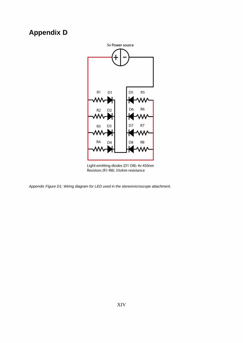
XIV

Appendix D

Appendix Figure D1: Wiring diagram for LED used in the stereomicroscope attachment.

vegard stürzinger

Documents