vector measure orthogonal sequences in spaces of square
TRANSCRIPT

Vector measure orthogonal sequences in spaces of square
integrable functions
Eduardo Jiménez Fernández
Departament de Matematica AplicadaUniversitat Politecnica de Valencia
VECTOR MEASURE ORTHOGONAL SEQUENCES
IN SPACES
OF
SQUARE INTEGRABLE FUNCTIONS
Ph.D. Dissertation
Author
Eduardo Jimenez Fernandez
Supervisors
Dr. Enrique Alfonso Sanchez PerezDr. Luıs Miguel Garcıa Raffi
November 2011
This editorial is member of the UNE, which guarantees the diffusion and commercialization of its publications at national and international level.
© Eduardo Jiménez Fernández, 2012
First Edition, 2012
© of the present edition: Editorial Universitat Politècnica de València www.editorial.upv.es ISBN: 978-84-8363-806-4 (printed version) Ref. editorial: 5518 Queda prohibida la reproducción, distribución, comercialización, transformación, y en general, cualquier otra forma de explotación, por cualquier procedimiento, de todo o parte de los contenidos de esta obra sin autorización expresa y por escrito de sus autores.
Don Enrique Alfonso Sanchez Perez , y Don Luıs Miguel GarcıaRaffi, profesores del Departamento de Matematica Aplicada de la UniversidadPolitecnica de Valencia,
CERTIFICAN que la presente memoria Vector measure or-thogonal sequences of spaces of square integrable functions ha sidorealizada bajo su direccion en el Departamento de Matematica Aplicada de laUniversidad Politecnica de Valencia, por Eduardo Jimenez Fernandez yconstituye su tesis para optar al grado de Doctor en Ciencias Matematicas.
Y para que ası conste, en cumplimiento de la legislacion vi-gente, presentamos ante el Departamento de Matematica Aplicada de la Uni-versidad Politecnica de Valencia, la referida Tesis Doctoral, firmando el presentecertificado.
En Valencia, a 27 de septiembre 2011
Fdo. Enrique Alfonso Sanchez Perez Fdo. Luıs Miguel Garcıa Raffi

Despues de un largo periplo, presento esta memoria que es el fruto de anosde trabajo y que finalmente concluyo no sin antes agradecer profundamente amis directores Enrique A. Sanchez Perez y Luis M. Garcıa Raffi todo el apoyorecibido en la realizacion de este trabajo. Quiero dar las gracias en especial alprofesor Jose M. Calabuig Rodrıguez y a la profesora Marıa Aranzazu Juan, porsus consejos y observaciones que han sido de gran utilidad.
Finalmente quiero expresar mi gratitud, a mi esposa Rosa que ha sufridodirectamente todas mis divagaciones, y a mis padres y hermana que desde elprimer dıa me ofrecieron todo su apoyo y animo.

To Marıa
Resum
Aquesta tesi doctoral s’emmarca dins de l’analisi dels subespais de successionsortogonals de funcions de quadrat integrable respecte d’una mesura vectorial quees numerablement aditiva i pren valors en un espai de Banach. La motivaciod’aquest treball es la generalitzacio dels arguments geometrics que proporcio-nen els procediments classics d’aproximacio als espais de Hilbert. La nociod’ortogonalitat representa un punt clau que permet el desenvolupament de lateoria de la convergencia de successions en aquests espais. Actualment, la con-vergencia gairebe per a tot punt, la convergencia en norma i la convergenciafeble son temes ben coneguts en la teoria d’espais de funcions de Hilbert.
Els espais de Banach de funcions L2(m) d’una mesura de vectorial m rep-resenten una amplia classe de reticles de Banach: cada reticle de Banach 2-convex ordre continu amb una unitat feble pot ser representat (a traves d’unisomorfisme d’ordre) com un espai L2(m) de una mesura vectorial adequada m.L’estructura integral que l’operador integracio proporciona en aquests espaispermet generalitzar arguments de ortogonalitat de la teoria d’espais de Hilbert,tot i que els espais L2(m) estan lluny de ser espais de Hilbert.
En el primer capıtol d’aquesta memoria s’introdueixen alguns conceptesbasics dels espais de Banach de funcions, integracio sobre mesures vectorialsi altres temes que seran necessaris al llarg de tot el treball. Es desenvolupenalguns resultats sobre la convergencia de successions en espais de Banach defuncions, igual que es mostren alguns procediments que seran de gran utilitat.Alguns arguments sobre ortogonalitat tambe son introduıts, tant en el context desuccesions de L2(m) com en les integrals d’aquestes successions quan la mesuravectorial m pren valors en un espai de Hilbert H. S’analitza la convergenciaincondicional de successions des del punt de vista abstracte dels espais de fun-cions integrables, i es proporciona una versio del metode de disjuntificacio deKadec i Pelczynsky per a mesures vectorials.
En el segon capıtol, es presenten formalment tres nocions d’ortogonalitatd’una successio respecte d’una mesura vectorial. La m−ortogonalitat feble,la (natural) m−ortogonalitat i la m−ortogonalitat forta, proporcionant tambealguns exemples que mostren la relacio amb problemes classics del analisi fun-cional. Tambe s’estudia la geometria d’aquestes successions.
En el capıtol 3 analitzem la convergencia gairebe per a tot punt de succes-sions que son febles m−ortogonals. El resultat mes rellevant d’aquesta seccioens mostra una versio general del teorema de Menchoff-Rademacher. A con-tinuacio es mostra un cas particular que involucra les c0-sumes d’un espai deHilbert amb la finalitat de mostrar les propietats de la convergencia gairebe pera tot punt.
Finalment, al capıtol 4 es desenvolupa una aplicacio concreta en el contextde les mesures vectorials. Es facilita un metode d’aproximacio respecte d’unamesura parametrica. Els principals elements d’aquest procediment son unasuccessio feble m−ortonormal i una funcio integrable Bochner que definira lanostra mesura, sobre la qual podrem calcular uns coeficients de Fourier - que enaquest cas seran funcions mesurables - per una determinada funcio de L2(m). Ifinalment, es mostraran algunes aplicacions d’aproximacio de senyals procedentsde dades experimentals en el camp de l’acustica.

Resumen
Esta tesis doctoral se enmarca dentro del analisis de los subespacios de suce-siones ortogonales de funciones de cuadrado integrable respecto de una medidavectorial que es numerablemente aditiva y toma valores en un espacio de Ba-nach. La motivacion de este trabajo es la generalizacion de los argumentosgeometricos que proporcionan los procedimientos clasicos de aproximacion enlos espacios de Hilbert. La nocion de ortogonalidad representa un punto claveque permite el desarrollo de la teorıa de la convergencia de sucesiones en estosespacios. Hoy en dıa, la convergencia casi por todas partes, la convergencia ennorma y la convergencia debil son temas bien conocidos en la teorıa de espaciosde funciones de Hilbert.
Los espacios de Banach de funciones L2(m) de una medida de vectorial mrepresentan una amplia clase de retıculos de Banach: cada retıculo de Banach2-convexo orden continuo con una unidad debil puede ser representado (a travesde un isomorfismo de orden) como un espacio L2(m) para una medida vectorialadecuada m. La estructura integral que el operador integracion proporciona enestos espacios permite generalizar argumentos de ortogonalidad de la teorıa delespacios de Hilbert, a pesar de que los espacios L2(m) estan lejos de ser espaciosde Hilbert.
En el primer capıtulo de esta memoria se introducen algunos conceptosbasicos de los espacios de Banach de funciones, integracion sobre medidas vec-toriales y otros temas que seran necesarios a lo largo de todo el trabajo. Sedesarrollan algunos resultados sobre la convergencia de sucesiones en espaciosde Banach de funciones, al igual que se muestran algunos procedimientos queseran de gran utilidad. Algunos argumentos sobre ortogonalidad tambien sonintroducidos, tanto en el contexto de sucesiones de L2(m) como en las integralesde estas sucesiones cuando la medida vectorial m toma valores en un espaciode Hilbert H. Se analiza la convergencia incondicional de sucesiones desde elpunto de vista abstracto de los espacios de funciones integrables, y se propor-ciona una version del metodo de disyuntificacion de Kadec y Pelczynsky paramedidas vectoriales.
En el segundo capıtulo, se presentan formalmente tres nociones de ortogo-nalidad de una sucesion respecto de una medida vectorial. La m−ortognalidad

debil, la (natural) m−ortogonalidad y la m−ortogonalidad fuerte, proporcio-nando tambien algunos ejemplos que muestran la relacion con problemas clasicosdel analisis funcional. Tambien se estudia la geometrıa de estas sucesiones.
En el capıtulo 3 analizamos la convergencia casi por todas partes de suce-siones que son debil m−ortogonales. El resultado mas relevante de esta seccionnos muestra una version general del teorema de Menchoff-Rademacher. A con-tinuacion se muestra un caso particular que involucra las c0-sumas de un espaciode Hilbert con el fin de mostrar las propiedades de la convergencia casi por todaspartes.
Finalmente, en el capıtulo 4 se desarrolla una aplicacion concreta en el con-texto de las medidas vectoriales. Se facilita un metodo de aproximacion respectode una medida parametrica. Los principales elementos de este procedimiento sonuna sucesion debil m−ortonormal y una funcion integrable Bochner que definiranuestra medida, sobre la cual podremos calcular unos coeficientes de Fourier –que en este caso seran funciones medibles– para una determinada funcion deL2(m). Y por ultimo, se mostraran algunas aplicaciones de aproximacion desenales procedentes de datos experimentales en el campo de la acustica.
Summary
This doctoral thesis is devoted to the analysis of orthogonal sequences in sub-spaces of spaces L2(m) of square integrable functions with respect to a Banachspace valued countably additive measure m. The motivation of our work isto generalize the geometric arguments that provide the classical approximationprocedures in Hilbert spaces. The notion of orthogonality lies in the center ofthe Hilbert space theory, and it allows to develop the theory of convergence ofsequences in these spaces. Almost everywhere convergence, norm convergenceand weak convergence are nowadays well known topics in the Hilbert space func-tion theory.
The Banach function spaces L2(m) of a vector measure m represent a broadclass of Banach lattices: each 2-convex order continuous Banach lattice with aweak unit can be represented (by means of an order isomorphism) as a spaceL2(m) for an adequate vector measure m. The integral structure that the vectormeasure integration provides in these spaces allows to generalize the orthogo-nality arguments of the Hilbert space theory, although the spaces L2(m) are farfrom being Hilbert spaces.
The first chapter of this memoir is devoted to introduce some fundamen-tal concepts on Banach function spaces, vector measure integration and othertopics that will be necessary in the rest of the work. Some results on conver-gence of sequences in Banach function spaces and Banach spaces are explained,and the general framework is established. Some orthogonality arguments arealready introduced, both for sequences in L2(m) and for the integrals of thesesequences when the vector measure m is Hilbert space valued. Unconditionalconvergence for sequences from the abstract point of view of the function spacesof integrable functions is analyzed, and a version of the Kadec and Pelczynskymethod for finding disjoint sequences for the vector measure setting is given.
In the second chapter three notions of orthogonality of a sequence withrespect to a vector measure are formally introduced, and the main characteri-zations of these sequences are given. Weak m-orthogonal sequences, (natural)m-orthogonal sequences and strongly m-orthogonal sequences are defined andstudied, providing also examples that show the relation with some classical prob-
lems in analysis. The geometry of these sets of sequences are also studied.
In Chapter 3 we analyze almost everywhere convergence of weak m-orthogonalsequences. Our main result is a general vector measure version of the Menchoff-Rademacher Theorem. A particular case involving c0-sums of Hilbert spaces isalso intensively studied in order to show the properties of the convergence.
Finally, Chapter 4 is devoted to show a concrete application. We develop anapproximation method with respect to a parametric measure based on our ideas.A Bochner integrable function and an weak m-orthonormal sequence are themain elements of our procedure, that allows to find the Fourier coefficients –thatare in this case measurable functions– for a given function in the space L2(m).Some applications for signal approximation for data coming from experimentalacoustics are also shown.

Contents
0.1 Motivation . . . . . . . . . . . . . . . . . . . . . . . . . . . . . . i0.2 Notes and remarks . . . . . . . . . . . . . . . . . . . . . . . . . . ii
0.2.1 Moment’s problem . . . . . . . . . . . . . . . . . . . . . . ii0.2.2 L2(m) spaces from the point of view of the vector measure
theory . . . . . . . . . . . . . . . . . . . . . . . . . . . . . iv0.3 Applications . . . . . . . . . . . . . . . . . . . . . . . . . . . . . . v0.4 The structure of the thesis . . . . . . . . . . . . . . . . . . . . . . vi
1 Notation and Preliminaries 11.1 Basic notions . . . . . . . . . . . . . . . . . . . . . . . . . . . . . 11.2 Unconditional basis in L2(m) . . . . . . . . . . . . . . . . . . . . 71.3 Kadec− Pelczynski decomposition . . . . . . . . . . . . . . . . 13
2 m−Orthogonal sequences with respect to a vector measure 192.1 m−Orthogonal sequences of functions with respect to a vector
measure . . . . . . . . . . . . . . . . . . . . . . . . . . . . . . . . 192.2 Weak m-orthogonal sequences . . . . . . . . . . . . . . . . . . . . 202.3 m−Orthogonal sequences . . . . . . . . . . . . . . . . . . . . . . 252.4 Strongly m−orthogonality . . . . . . . . . . . . . . . . . . . . . . 31
3 The Menchoff-Rademacher Theorem for L2(m) 393.1 About almost everywhere convergence of sequences in L2(m) . . 413.2 The Menchoff-Rademacher Theorem for
weak m-orthogonal sequences . . . . . . . . . . . . . . . . . . . . 443.3 Almost everywhere convergence in c0-sums of L2(µ) spaces . . . 50
4 Pointwise dependent Fourier coefficients 534.1 Pointwise dependent Fourier coefficients . . . . . . . . . . . . . . 544.2 Continuity of the pointwise dependent
Fourier coefficients . . . . . . . . . . . . . . . . . . . . . . . . . . 624.3 An example of approximation with finite m-orthogonal sequences 654.4 Application to acoustic data . . . . . . . . . . . . . . . . . . . . . 72
References 77

Introduction
0.1 Motivation
The notion of orthogonality lies in the center of the Hilbert and Banach spaces
theory and it has a clear geometrical meaning. Even for the case of finite di-
mensional spaces with the Euclidean norm the notion of orthogonality is deeply
connected with the topological properties of the space and mainly with the no-
tion of best approximation. The same relation can be extended to the setting of
the Hilbert spaces, which has as a canonical example the space L2[0, 1]. In the
year 2000, a new class of Banach function spaces was introduced: the spaces
Lp(m) of p-integrable functions with respect to a vector measure m. Those
spaces are rather general, since they represent the class of all order continuous
p-convex Banach function spaces with a weak unit. So, the space L2(m) is 2-
convex, but it is far of having a Hilbert space structure. However, and due to its
integration structure, several notions of orthogonality still make sense in it. The
geometric consequences of these notions and some applications in the context of
the best approximation and Fourier analysis has been studied in recent years,
as the reader can notice by checking the references in this memoir.
The aim of this thesis is to analyze and to show some applications of the
three notions of vector measure orthogonality that has been introduced in the
literature up to this moment, and to develop a systematic theory of vector
measure orthogonality including all these cases. This of course imply to study
the structure of the spaces L2(m) of a vector measure and the main properties
i

ii Introduction
of the integration map restricted to these spaces.
One of the basic concepts that leads to the one of vector measure orthog-
onality is the vector measure duality. It consists on considering the duality
induced by the bilinear form defined by the integration map, i.e. if m : Σ→ X
is a countably additive vector measure with values in the Banach space X and
1 = 1/p+1/q, the integral defines a bilinear form Bm : Lp(m)×Lq(m)→ X by
Bm(f, g) :=∫fg dm. Duality results can be found in [30, 31, 59, 60, 61]. These
duality results, that provide for instance a representation of the dual space, are
applied in this thesis in the symmetric case given by p = 2.
0.2 Notes and remarks
In this section we are going to show the concept of orthogonality with respect
to a vector measure has its roots in the XIX century.
0.2.1 Moment’s problem
The orthogonality with respect to a vector measure can be easily related to some
classical mathematical problems, as the so called Moment´s problem. Actually,
as will be shown in Chapter 2, orthogonality with respect to a vector measure is a
general setting that includes for instance orthogonality of a sequence of functions
with respect to a family of measures, or what is called in statistics, a parametric
measure. The analysis of the properties of functions that are orthogonal with
respect to a family of measures has a long mathematical history, for instance
regarding orthogonal polynomials. In 1885 Tchebyshev established the following
question. If the relations∫ ∞−∞
xnω(x)dx =
∫ ∞−∞
xne−x2
dx
holds for all n ∈ N this implies that ω(x) = e−x2
? The answer is yes and today
we say that the problem is determinate.

Introduction iii
There are different points of view to try to solve this problem. The first pro-
cedure was developed by Stieljes in 1894 (see [62]). According Dieudonne (see
[26]), the moment’s problem is no stranger to the birth of Banach theory. M.
Riesz in [52] provided a solution using the Helly’s Representation Theorem (see
[13]) , and Nevalinna introduced a new tool into the analytic function theory in
[4] for trying to solve this problem.
When the problem is not determined we obtain a family of scalars measures
such that∫∞−∞ xnω(x)dx = Sn, n = 0, 1, 2... have the same moments. At the
end of the 19th century some relevant cases of families of polynomials that
are orthogonal with respect to a large set of scalar measures —indeterminate
measures— were known. The first example of such an indeterminate measure
was presented by Stieltjes in 1894 (see [62]). If we start with the two following
integrals ∫ ∞0
e−t2
dt =√π and
∫ ∞0
e−t2
sin(2πt)dt = 0
and now we do the next transformation t = ln(x)− (n+ 1)/2, then
e−t2
= e− ln2(x)xn+1e−(n+1)2/4 and dt =dx
x.
So we obtain∫ ∞0
xne− ln2(x)dx =√πe(n+1)2/4,
∫ ∞0
xne− ln2(x) sin(2π ln(x))dx = 0.
Then if we multiply the second integral by a constant K ∈ R and we add the
first integral, we obtain∫ ∞0
e− ln2(x)xn[1 +K sin(2π ln(x))]dx =√πe(n+1)2/4.
If we take |K| < 1 then e− ln2(x)[1 + K sin(2π ln(x))] > 0 is a positive function
for all x ∈ [0,∞[, thus FK(y) =∫ y
0e− ln2(x)xn[1 +K sin(2π ln(x))]dx is a family
of non decreasing distributions with support into [0,∞[ which have the same
moments√πe(n+1)2/4. The polynomials that are orthogonal with respect to
this class of measures are a special case of the Stieltjes-Wigert polynomials.
Using the family (FK)K∈[−1,1] of distributions, a vector measure can be defined
in an easy way (see Example 2.3.2). In general this construction can be done
for abstract sets of measures —for instance, parametric models in statistics—,
and then to find sequences of functions that are orthogonal for all the elements

iv Introduction
of a family of measures is equivalent to the problem of finding sequences that
are orthogonal with respect to a vector measure.
Our main references on measure spaces, scalar measures, integration with
respect to scalar measures, vector measures and function spaces are [25, 33,
42, 49]. The reader can find general definitions and results on integration with
respect to vector measures and the related spaces of m-integrable functions
L1(m) in [15, 40, 41].
0.2.2 L2(m) spaces from the point of view of the vectormeasure theory
From the point of view of the integration with respect to a vector measure, the
properties of the integration map that are nowadays well known provide relevant
information with important consequences on the properties of the orthogonal
sequences in the spaces L2(m). Compactness properties of the integration map
—weak compactness, compactness, complete continuity— have direct conse-
quences on the structure of the corresponding spaces of integrable functions.
For instance, if the integration operator is compact, the corresponding space is
order isomorphic to the L1-space of the variation |m|, i.e. an L1-space. Con-
sequently, in this case L2(m) is order isomorphic to the Hilbert space L2(|m|)(see Proposition 3.48 in [49] and the references therein). Regarding weak com-
pactness, it is also known that the integration map restricted to L2(m) is always
weakly compact (see [28, 29, 60]). Also, the geometric properties of the integra-
tion map will be used in this thesis. For instance, p-concavity of the integration
map restricted to Lp(m) implies that this space is order isomorphic to an Lp-
space (see [9, 16, 17]).
In recent years, some applications of the spaces L2(m) have been developed
in the setting of the function approximation. In particular, the geometry of the
strongly m-orthogonal sequences is well known and can be found in the papers
[34, 48, 59]. Some applications on function approximation of m-orthogonal
sequences were developed also in the papers [34, 35, 36].

Introduction v
Some results that follows the general research program of analyzing conver-
gence of sequences in the spaces Lp of a vector measure has been published yet,
and do not constitute a part of this memoir, although they are closely related.
In this direction, we must mention two papers. The first one, [10], analyzes and
improves some known results on decompositions of unconditional convergence
of sequences in Banach function spaces using the structure of the spaces Lp(m).
The second one, [37], provides a general analysis of the Komlos property re-
garding a.e. convergence of the Cesaro sums in spaces of measurable functions.
In this case, a most general theory of vector measure integration involving δ-
rings is used in order to establish how far, in the scale of ideals of measurable
functions, the Fatou property and the Komlos property are equivalent.
Those results have not being included in this memoir because they do not
use any orthogonality argument, although the subject that they deal with is very
much concerned with the one of the work presented in this memoir: different
aspects of the convergence of sequences in the spaces L2 of a vector measure.
0.3 Applications
The last part of the thesis (Chapter 4) is devoted to show some new applications
of the spaces L2(m) in the setting of the function approximation. In particular,
we develop an approximation structure that consists of providing a parametric
set of measures by means of the action of a Bochner integrable function with
the vector measure. A suitable error criterion is defined and the corresponding
approximation formulae are given. This leads to a non linear approximation for
a given function of L2(µ), that has the advantage that a small orthogonal set of
functions is enough for obtaining a good approximation, improving the one that
is obtained when the Hilbert space structure is used. Some examples are given,
and a concrete application to representation of acoustic signals is developed.
vi Introduction
0.4 The structure of the thesis
Chapter 1 is devoted to recall and adapt some well known results on the behavior
of sequences in Banach function spaces. An adapted version of the Bessaga−Pelczynski for weakly null sequences (see [7]) and the Kadec − Pelczynski
method for obtaining disjoint sequences that approximate special sequences is
given (see [32, 38]).
In Chapter 2, the three notions of m-orthogonality are given and analyzed,
showing some examples and existence results for such sequences in the L2(m)
spaces.
Chapter 3 shows how the Menchoff-Rademacher results on almost every-
where convergence of sequences can be adapted and improved for the case of
m-orthogonal sequences, that comes from the fact that the vector measure or-
thogonality is stronger than the scalar notion. The last chapter provides the
applications of the theory that has been explained above.

Chapter 1
Notation and Preliminaries
1.1 Basic notions
In this chapter, we introduce the concepts and results used throughout the
memory about Banach function spaces and integration of real functions with
respect to a vector measure. We will use standard Banach and function space
notation; our main references are [25, 42, 64]. Let X be a Banach space. We
will denote by BX the unit ball of X, that is BX := x ∈ X : ‖x‖ = 1. X ′ is
the topological dual of X and BX′ its unit ball. If 1 ≤ p ≤ ∞, we write q for
the (extended) real number satisfying 1/p+ 1/q = 1. A Banach space X is said
of type p for some 1 < p ≤ 2 respectively, of cotype q for some q ≥ 2, if there
exists a constant M < ∞ so that, for every finite set of vectors xjnj=1 in X,
we have ∫ 1
0
‖n∑i=1
rj(t)xj‖dt ≤M(
n∑j=1
‖xj‖p)1/p,
respectively ∫ 1
0
‖n∑i=1
rj(t)xj‖dt ≥1
M(
n∑j=1
‖xj‖q)1/q,
where rjj denotes the sequence of the Rademacher functions. The Hilbert
spaces have the best possible type and cotype, i.e. are simultaneously of type 2
1

2 Chapter 1. Notation and Preliminaries
and cotype 2 and the converse of this assertion is also true (see [42, 1.e.12]).
Let X and Y be Banach spaces. An operator T : X → Y is 2-absolutely
summing if there exists a constant C > 0 such that for every finite sequence
x1, ..., xn ∈ X,
(
n∑i=1
‖T (xi)‖2)12 ≤ C sup(
n∑i=1
|〈xi, x′〉|2)12 : x′ ∈ X ′, ‖x′‖ ≤ 1. (1.1)
We define the 2-summing norm of T as
π2(T ) = infC : (1.1) holds for all xini=1 ⊂ X, n ∈ N. (1.2)
Let X be a Banach lattice, that is a real Banach space endowed with a norm
‖ · ‖ and a partial order ≤ such that
(1) if x, y, z ∈ X with x ≤ y, then x+ z ≤ y + z,
(2) if x, y ∈ X with x ≤ y, then αx ≤ αy for all α > 0,
(3) for x, y ∈ X, there exists the supremum of x and y with respect to the
order,
(4) if x, y ∈ X with |x| ≤ |y|, then ‖x‖ ≤ ‖y‖, where |x| = supx,−x is the
modulus of x.
Note that (3) implies that also there exists the infimum of every x, y ∈ X. The
supremum and the infimum of two elements x and y of X are usually denoted
by x∨ y and x∧ y respectively. A weak unit of X is an element 0 ≤ e ∈ X such
that x ∧ e = 0 implies that x = 0.
We say that a Banach lattice X is order continuous if for every sequence xnn ⊂X with xn ↓ 0 it follows that ‖xn‖ ↓ 0. We say that X has the Fatou property
if for every net (xτ ) ⊂ X with 0 ≤ xτ ↑ such that sup ‖xτ‖ <∞ if follows that
there exists x = supxτ in X and ‖x‖ = sup ‖xτ‖. Let T : X → Y be a linear
operator between two Banach lattices. The operator T is said to be positive
if T (x) ≥ 0 whenever 0 ≤ x ∈ X. Every positive linear operator between two
Banach lattices is continuous. We will say that T is an order isomorphism if it is
one to one, onto and satisfies that T (x∧y) = T (x)∧T (y) for all x, y ∈ X. In this
case, T is continuous as it is positive and also satisfies T (x ∨ y) = T (x) ∨ T (y)
for all x, y ∈ X. If moreover, ‖T (x)‖Y = ‖x‖X for all x ∈ X, we will say that
T is an order isometry. Let E and F be Banach lattices and 1 ≤ p < ∞. An
operator T : E → F is p-concave if there is a constant K > 0 such that for

1.1 Basic notions 3
every finite set x1, x2, ..., xn ∈ E, it follows
(
n∑i=1
‖ T (xi) ‖p)1p ≤ K ‖ (
n∑i=1
| xi |p)1p ‖ . (1.3)
The infimum of such constants K is the p-concavity constant of the operator.
An operator T : E → F is p-convex if there is a constant K > 0 such that for
each finite set x1, x2, ..., xn ∈ E, it follows
‖ (n∑i=1
| T (xi) |p)1p ‖≤ K(
n∑i=1
‖ xi ‖p)1p . (1.4)
As in the case of p-concavity, the infimum of such constants K is the p-convexity
constant of T . A Banach lattice E is p-concave (p-convex) if the identity map
Id : E → E is p-concave (p-convex). Throughout the memoir we will consider
Banach function spaces as Banach lattices with the usual µ-a.e. pointwise order.
For the aim of simplicity, we will assume that the corresponding p-concavity/p-
convexity constants of the spaces are 1; it is known that each r-convex and
s-concave Banach lattice, 1 ≤ r ≤ s ≤ ∞, can be renormed equivalently so that
with the new norm, the r-convexity and s-concavity constants are both equal
to 1 (see [42, 1.d.8]).
Let (Ω,Σ, µ) be a σ-finite measure space. Following the definition in [42, p.28],
a Banach space X(µ) of (classes of) locally µ-integrable real functions is said
to be a Banach function space over µ (Kothe function space) if it satisfies the
next two properties.
• If f is measurable and g ∈ X(µ) such that |f(w)| ≤ |g(w)| µ−a.e. on Ω,
then f ∈ X(µ) and ‖f‖ ≤ ‖g‖.
• If A ∈ Σ, and µ(A) < ∞, then the characteristic function χA belongs to
X(µ).
We write as usual `p, 1 ≤ p < ∞, and c0 for the classical sequence spaces,
and ‖.‖p, ‖.‖0 for the corresponding norms. The sequence spaces that we deal
with (L, ` ...) are assumed to be such kind of spaces. Thus, we will consider
spaces of real functions on the standard measure space on the set of natural
numbers N with an unconditional normalized basis with unconditional constant
1. We will write ei, i ∈ N, for the elements of the canonical basis of the space.
Moreover, we also assume that its dual space can be represented as a sequence
space, i.e. its elements can be written as sequences τii, and the duality is
given by 〈τi, λi〉 =∑∞i=1 τiλi, λii ∈ L. For instance, this always happens
4 Chapter 1. Notation and Preliminaries
when the space is order continuous (see the comments that follow Definition
1.b.17 in [42]). We will use the following construction for the particular case of
sequence spaces (i.e. the measure is the discrete one on the set of the natural
numbers). Let (Ω,Σ) be a measurable space and X a Banach space. Throughout
the memory m : Σ → X will be a countably additive vector measure, i.e.
m(∪∞n=1An) =∑∞n=1 m(An) in the norm topology of X for all sequences Ann
of pairwise disjoint sets of Σ. It is well known that every Banach space valued
countably additive vector measure on a σ−algebra is bounded. We say that
a countably vector measure m : Σ → X, where X is a Banach lattice, is
positive if m(A) ≥ 0 for all A ∈ Σ. For each element x′ ∈ X ′ the formula
〈m, x′〉(A) := 〈m(A), x′〉, A ∈ Σ, defines a (countably additive) scalar measure.
We write |〈m, x′〉| for its variation, i.e. |〈m, x′〉|(A) := sup∑B∈Π |〈m(B), x′〉|
for A ∈ Σ, where the supremum is computed over all finite measurable partitions
Π of A. Sometimes we write mx′ for 〈m, x′〉. We say that an element x′ ∈ X ′
is m−positive if the scalar measure mx′ is positive, i.e. |mx′ | = mx′ . We write
(X ′)+m for the set of these elements. The semivariation of m is the extended
nonnegative function ‖m‖ whose value on a set A ∈ Σ is given by:
‖m‖(A) = sup|〈m, x′〉|(A) : x′ ∈ X ′, ‖x′‖ ≤ 1.
Direct computations show that the variation |m| is a monotone countably ad-
ditive function on Σ, while the semivariation ‖m‖ is a monotone subadditive
function on Σ, and for each A ∈ Σ we have that ‖m‖(A) ≤ |m|(A). A vector
measure m defined on a σ−algebra is always bounded, i.e. m(A) < ∞ for all
A ∈ Σ. In general, a vector measure m is of bounded semivariation on Ω if and
only if its range is bounded in X, as for A ∈ Σ, sup‖m(B)‖ : A ⊇ B ∈ Σ ≤‖m‖(A) ≤ 4 sup‖m(B)‖ : A ⊇ B ∈ Σ. As usual, we say that a sequence
of functions converges |〈m, x′〉|-almost everywhere if it converges pointwise in
a set A ∈ Σ such that |〈m, x′〉|(Ω \ A) = 0. A sequence converges m-almost
everywhere if it converges in a set A that satisfies that the semivariation of m
in Ω \A is 0.
We will say that a scalar positive measure µ is equivalent to m if
limµ(A)→0
‖m‖(A) = 0 and lim‖m‖(A)→0
µ(A) = 0.
The measure m is absolutely continuous with respect to µ if limµ(A)→0 m(A) =
0; in this case we write m µ and we say that µ is a control measure for m.
Countably additive vector measures always have a control measure. The Bartle,

1.1 Basic notions 5
Dunford and Schwartz theorem (see [25, Ch.I,2, Corollary 6]) produces a finite
nonnegative real-valued measure µ on Σ such that m µ. Furthermore, it is
known that there exists always an element x′ ∈ X ′ such that m |〈m, x′〉| and
so m |〈m, x′〉| is a control measure for m. We call such a scalar measure a
Rybakov measure for m (see [25, Ch.IX,2]). If |〈m, x′〉| is a Rybakov measure
for m, then a sequence of functions converges m-almost everywhere if and only
if it converges |〈m, x′〉|-almost everywhere. Notice that if m is positive and x′
is a positive element of the Banach lattice X ′, then |〈m, x′〉| = 〈m, x′〉.The space L1(m) of integrable functions with respect to m is a Banach function
space over any Rybakov measure µ for m (see [15, 42]). The elements of this
space are (classes of µ-a.e. measurable) functions f that are integrable with
respect to each scalar measure 〈m, x′〉, and for every A ∈ Σ there is an element∫Afdm ∈ X such that 〈
∫Afdm, x′〉 =
∫Afd〈m, x′〉 for every x′ ∈ X ′. When
no explicit reference is needed, we write∫fdm instead of
∫Ωfdm. The reader
can find the definitions and fundamental results concerning the space L1(m) in
[15, 40].
The space of (classes of µ−a.e. equal) real measurable functions on (Ω,Σ)
is denoted by L0(µ). The formula
| ‖f‖ |L1(m):= supA∈Σ
∥∥∥∥∫A
fdm
∥∥∥∥X
, f ∈ L1(m).
where ‖ · ‖X denotes the norm of X, gives a norm on L1(m), since functions
that are equal m−a.e. are identified. Moreover,
| ‖f‖ |L1(m)≤ ‖f‖L1(m) ≤ 2 | ‖f‖ |L1(m) for every f ∈ L1(m).
The space L1(m) of m−a.e. equal m−integrable functions is a Banach lattice
endowed with the norm ‖ · ‖L1(m) and the m−a.e. order. It is an ideal of
measurable functions, that is |f | ≤ |g| m−a.e. with f ∈ L0(µ) and g ∈ L1(m),
then f ∈ L1(m) and an order continuous Banach lattice.
We build the spaces Lp(m), that are also order continuous Banach function
spaces over the space (Ω,Σ, |mx′0|) with weak unit where |mx′0
| is a Rybakov
measure. We say that a measurable function f : Ω → R is p−integrable with
respect to m if |f |p ∈ L1(m) with the norm
‖f‖Lp(m) := ‖|f |p‖1p
L1(m), f ∈ Lp(m).

6 Chapter 1. Notation and Preliminaries
We denote the integration operator associated to the vector measure m by
Im : Lp(m) −→ Xf 7−→ Im(f) =
∫Afdm
.
The properties of the integration map associated to a vector measure has been
largely studied in several recent papers (see [22, 49]).
Before introducing several results concerning basic sequences, we provide
a representation of the dual space of Lp(m) in terms of the space Lq(m) (m
is a countably additive vector measure), as in the case of classical Lp-spaces.
It is well know that the dual of Lp coincides with Lq only in the case that
m is a scalar measure. Let L(Lp(m), X) be the subspace of all the operators
that satisfy Theorem 2.2 [30], i.e. that can be identified (isometrically and
isomorphically) with functions of Lq(m). Indeed Lq(m) is always the dual of
a certain topological tensor product. In the same paper, the autors prove the
following result: the spaces (((Lp(m) ⊗ X ′)/ keru, τu)′, ‖ · ‖u) and (Lq(m), ‖ ·‖Lq(m)) are isometrically isomorphic if and only if the unit ball of Lq(m) is
m−weakly compact, where u(z) = sup‖g‖Lq(m)≤1 |∑ni=1〈
∫figdm, x′i〉| if z =∑n
i=1 fi ⊗ x′i ∈ Lp(m)⊗X ′ and the quotient space (Lp(m)⊗X ′)/ keru define
the quotient topology τu generated by the seminorm u([z]) := u(z). Since
the m-weak topology is weaker than the weak topology of the space Lp(m),
the compactness property required in the above result is satisfied if the space
Lq(m) is reflexive. Another prove of this result can be found in [31]. Some
results regarding reflexivity of this space may be found in [28]. We recall that
a Banach lattice X is a KB-space whenever every norm bounded, positive,
increasing sequence is norm convergent, then it is known that for q > 1 Lq(m)
is reflexive if and only if Lq(m) is a KB-space, and a Banach lattice is a KB
space if and only if X has the Fatou property and is an order continuous Banach
lattice, so Lq(m) is reflexive if and only if Lq(m) has the Fatou property.
In this memoir we deal with sequences of functions in L2(m). If 〈m, x′〉 is
a Rybakov measure for m, then the inclusion map ix′ : L2(m) → L2(|〈m, x′〉|)is well-defined and continuous; in fact, even if x′ do not define a Rybakov
measure this identification map is well-defined and continuous, although it is not
injective. In this work we only need some particular properties of the functions
in L2(m). For instance, if f, g are functions in L2(m), we use the fact that the
product fg is m-integrable (see [28, 49] or [60]).

1.2 Unconditional basis in L2(m) 7
If L0(µ) is the space of (classes of µ-a.e. equal) real measurable functions,
0 < r <∞ and E(µ) is a Banach function space, we define the r-power of E(µ)
as the space
E(µ)[r] := x ∈ L0(µ) : |x|1/r ∈ E(µ)
endowed with the (quasi-)norm ‖x‖E[r]:= ‖|x|1/r‖rE . The space E(µ)[r] is always
a Kothe function space when 0 < r ≤ 1 and for r > 1 it is so whenever E(µ) is r-
convex; in this case the expression above gives a norm if the r-convexity constant
is 1 (see [19, 49] for the basic properties of r-powers of Kothe function Banach
spaces). For instance, if m is a countably vector measure, the space L2(m)
above can be written as the 1/2-power of L1(m), i.e. L2(m) = (L1(m))[1/2].
1.2 Unconditional basis in L2(m)
A sequence xn∞n=1 in a Banach space X is called a Schauder basis of X if there
exists a unique sequence of scalars αn∞n=1 such that x = limn→∞∑nk=1 αkxk
for all x ∈ X. A sequence xn∞n=1 which is a Schauder basis of its closed span is
called a basic sequence. A series∑∞n=1 xn in a Banach spaceX is unconditionally
convergent if for every permutation σ : N→ N the series∑∞n=1 xσ(n) converges.
A space with a basis is always separable. The most of the natural separable
spaces have bases, although Pel Enflo [27] was the first who found that there
are separable Banach spaces without bases, looked inside c0. The fact that a
separable Banach space has a basis does provide some structural information
about the space. It must be pointed out that finding a basis for a well know
space is sometimes difficult. For instance, in the case of the classical separable
sequence spaces c0 and `p (1 ≤ p <∞), the sequence en∞n=1 of unit coordinate
vectors en = (0, 0, ..., 0, 1(n-th place), 0, ...) is a basis. In the case of the space of
convergent sequences c, if we denote 1 = (1, 1, ...) then the sequence (1, e1, e2, ...)
is a basis for c. In the case of C[0, 1], the Schauder basis is a basis for this
space, generally if n ≥ 1 and 1 ≤ i ≤ 2n, then the sequence f1(t) = 1, f2(t) =
t, f3(t) = 2tχ[0,1/2](t) + 2(2− t)χ[1/2,1], ..., f2n+i+1(t) = f3(2nt+ 1− i) whenever
2n + n − i ∈ [0, 1] is a Schauder basis, see Figure 1.1. In the case of Lp[0, 1],
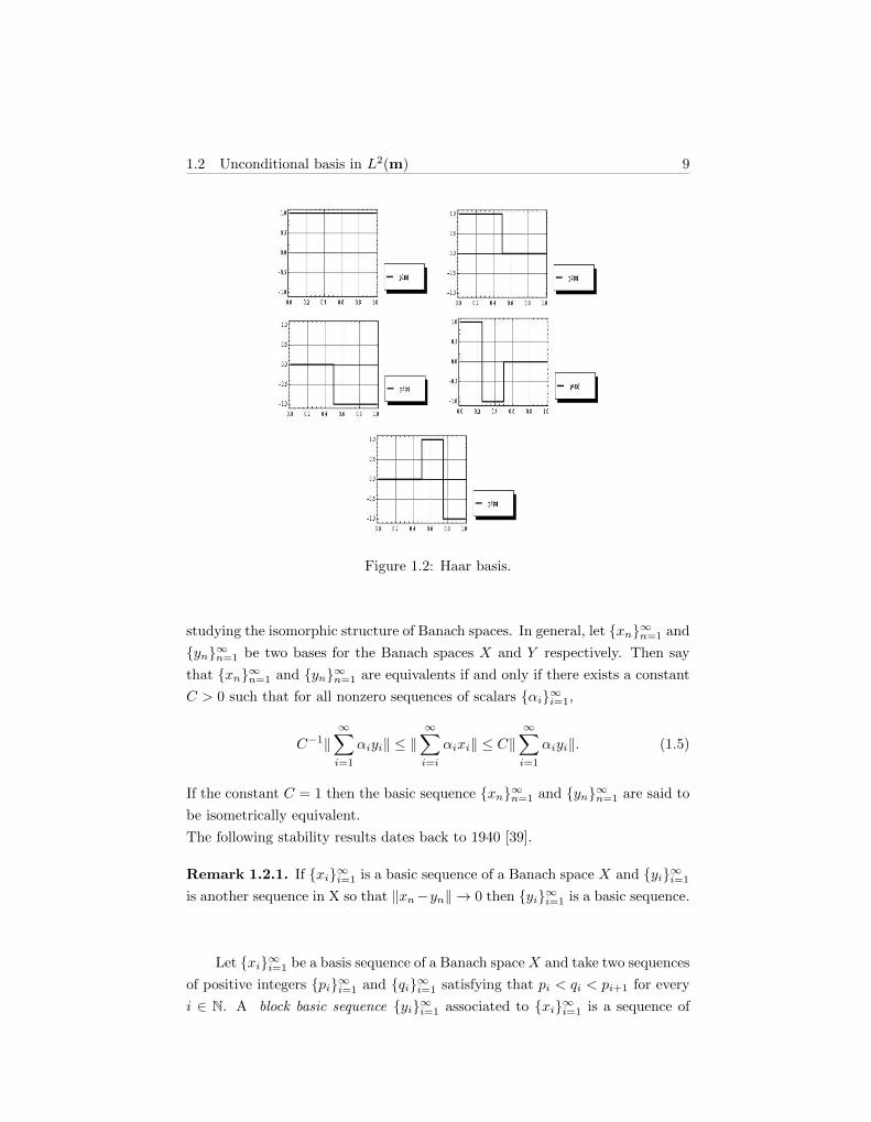
where 1 ≤ p <∞, the Haar system is a basis for this space, see 1.2. It is given

8 Chapter 1. Notation and Preliminaries
Figure 1.1: Schauder basis.
by
f0(t) = 1,
f2n+i(t) = χ[(2i−2)/2n+1,(2i−1)/2n+1](t)− χ[(2i−1)/2n+1,2i/2n+1](t),
if n ≥ 1 and 1 ≤ i ≤ 2n, and therefore if 1 < p <∞ it is an unconditional basis.
For the case of vector measures, there are examples such that the space of square
integrable with respect to a particular vector measure is known, for instance, if
m : Σ −→ L2[0, 1] and m(A) = χ(A) then L2(m) = L4[0, 1]. For this case the
Haar system is a basis for L2(m). For the case of the spaces L1(m) it is also
possible to find criteria for obtaining basic sequences, for instance Theorem 3,
[15]. In fact the Haar system is a basis for all Lp(µ), 1 ≤ p < ∞ (see Chapter
5, [24]).
We use standard Banach function space notation. Let xnn be a ba-
sic sequence. The symbol [xn] denote the smallest closed linear set spanned
upon the elements xn∞n=1 ⊂ X. The projections Pn : X → X defined by
Pn(∑∞i=1 αixi) =
∑ni=1 αixi are bounded operators and supn ‖Pn‖ < ∞. The
number K = supn ‖Pn‖ is called the basic constant of xn∞n=1. Equivalence of
basic sequences (and in particular of bases) will become a powerful technique for
1.2 Unconditional basis in L2(m) 9
Figure 1.2: Haar basis.
studying the isomorphic structure of Banach spaces. In general, let xn∞n=1 and
yn∞n=1 be two bases for the Banach spaces X and Y respectively. Then say
that xn∞n=1 and yn∞n=1 are equivalents if and only if there exists a constant
C > 0 such that for all nonzero sequences of scalars αi∞i=1,
C−1‖∞∑i=1
αiyi‖ ≤ ‖∞∑i=i
αixi‖ ≤ C‖∞∑i=1
αiyi‖. (1.5)
If the constant C = 1 then the basic sequence xn∞n=1 and yn∞n=1 are said to
be isometrically equivalent.
The following stability results dates back to 1940 [39].
Remark 1.2.1. If xi∞i=1 is a basic sequence of a Banach space X and yi∞i=1
is another sequence in X so that ‖xn−yn‖ → 0 then yi∞i=1 is a basic sequence.
Let xi∞i=1 be a basis sequence of a Banach space X and take two sequences
of positive integers pi∞i=1 and qi∞i=1 satisfying that pi < qi < pi+1 for every
i ∈ N. A block basic sequence yi∞i=1 associated to xi∞i=1 is a sequence of

10 Chapter 1. Notation and Preliminaries
vectors of X defined as finite linear combinations as
yi =
qi∑k=pi
αi,kxk,
where αi,k are real numbers (see also [24], Ch.V for the definition of block basic
sequence and also for the standard definition of equivalence between basis). Let
S be a subspace of X, S is called complemented in X if and only if there exists
a continuous projection from S onto X.
Fundamental to the study of bases in a separable Hilbert space H is the
notion of a biorthogonal system. If n,m are indexes of a set I, we write δn,m
for the Kronecker’s delta as usual. Two sequences xnn and ynn of elements
from H are said to be biorthogonal if 〈xn, ym〉 = δn,m.
Now, we consider the particular case when X is a space of 2−integrable
functions with respect to a vector measure m. In this case, the question of how
to recognize a basic sequence arises. The following remark provide a basic test
for recognizing a basis in a subspace of L2(m), (see Theorem 1. Ch.V [24]).
Remark 1.2.2. Let fn∞n=1 be a sequence of non zero functions in L2(m),
then in order fn∞n=1 to be a basic sequence, it is both necessary and sufficient
that there exists a positive finite constant K so that for any choice of scalars
αi∞i=1 and any integers m < n we have∥∥∥∥∥m∑i=1
αifi
∥∥∥∥∥L2(m)
≤ K
∥∥∥∥∥n∑i=1
αifi
∥∥∥∥∥L2(m)
. (1.6)
For instance, if m : Σ→ X is a positive vector measure, ‖f‖L2(m) = ‖∫|f |2‖1/2X
for all f ∈ L2(m) (see [23]), and so the criterion above can be written as follows.
For any finite sequences of scalars αi∞i=1 and any integers m < n,∥∥∥∥∥∫
(
m∑i=1
αifi)2dm
∥∥∥∥∥X
≤ K2
∥∥∥∥∥∫
(
n∑i=1
αifi)2dm
∥∥∥∥∥X
. (1.7)
In Chapter 2 we will provide the adequate requirements on fi∞i=1 in order to
obtain 1.7 that is equivalent to∥∥∥∥∥m∑i=1
α2i
∫f2i dm
∥∥∥∥∥X
≤ K2
∥∥∥∥∥n∑i=1
α2i
∫f2i dm
∥∥∥∥∥X
. (1.8)

1.2 Unconditional basis in L2(m) 11
Let S be a subspace of L2(m) with a normalized basis fn∞n=1, if we
perturb each element fn ∈ S by a sufficiently small vector we still get a basis
and the perturbed basis is equivalent to the original one, see (Proposition 1.a.9,
Vol I, [42]). The following remark show this.
Remark 1.2.3. Let xn∞n=1 be a normalized basis of a Banach space X with a
basis constant K. Let yn∞n=1 be a sequence of vectors in X with∑∞n=1 ‖xn−
yn‖ < 1/(2K). Then yn∞n=1 is a basis of X which is equivalent to xn∞n=1.
In what follows we consider vector measures which take values in Hilbert
spaces. We present a version of a principle for selecting basic sequences due to
Bessaga and Pelczynski (Corollaries 1.2.4 and 2.4.3 below and see also [7]).
We will consider first properties of the range of the vector measure and not of
the space L2(m).
Corollary 1.2.4. Let H be a Hilbert space and let m : Σ −→ H be a count-
ably additive vector measure. Let en∞n=1 be a basic sequence of H and e′nnbe a biorthogonal sequence to enn. If the sequence
∫f2ndm
∞n=1
fulfills the
condition∞∑n=1
∥∥en − ∫ f2ndm
∥∥H‖e′n‖H = δ < 1,
then∫
f2ndm
∞n=1
is a basic sequence which is equivalent to en.
Proof. For arbitrary integer i, p, q such that i < p < q, we have
|αi| = |e′i(p∑j=1
αjej)| ≤ ‖p∑j=1
αjej‖H‖e′i‖H .
From the above expression, we obtain
‖p∑j=1
αj(
∫f2j dm)‖H ≤ ‖
p∑j=1
αjej‖H + ‖p∑j=1
αj(ej −∫f2j dm)‖H
≤ ‖p∑j=1
αjej‖H +
p∑j=1
|αj |∥∥ej − ∫ f2
j dm∥∥H
≤ ‖p∑j=1
αjej‖H +
∞∑i=1
|αi|∥∥ei − ∫ f2
i dm∥∥H
≤ ‖p∑j=1
αjej‖H +
∞∑i=1
‖p∑j=1
αjej‖H‖e′i‖H‖ei −∫f2i dm‖H
12 Chapter 1. Notation and Preliminaries
≤ (1 + δ)‖p∑j=1
αjej‖H ,
and using the same computations that above, we obtain
‖q∑j=1
αj(
∫f2j dm)‖H ≥ |‖
q∑j=1
αjej‖H − ‖q∑j=1
αj(ej −∫f2j dm)‖H |
≥ (1− δ)‖q∑j=1
αjej‖H .
Hence
‖p∑j=1
αj(
∫f2j dm)‖H ≤ K
1 + δ
1− δ‖
q∑j=1
αj(
∫f2j dm)‖H .
Remark 1.2.5. In general, if we take xn∞n=1 a weakly null, normalized se-
quence in a Banach space X then xn∞n=1 admits a subsequence that is a basic
sequence, (see Bessaga-Pelczynski Selection Principle theorem [24]).
Example 1.2.6. Consider the Lebesgue measure space ([0,∞),Σ, dx) and de-
fine the positive vector measure ν : Σ→ c0 as
ν(A) =
∞∑n=0
(∫A∩[n,n+1]
(x− n)ndx
)en.
It is clearly countably additive and then the corresponding space L2(ν) is well-
defined. If f ∈ L1(ν) then∫fdν =
∫[n,n+1]
f(x)(x − n)ndx∞n=1 ∈ c0. Con-
sider now the sequence of functions fk∞k=0 = e−k(x−k)/2χ[k,∞)(x)∞k=0, then
f2k (x) = e−k(x−k)χ[k,∞)(x) ∈ L1(ν) and so fk ∈ L2(ν).
‖fk‖2L2(ν) =
∥∥∥∥∥∫
[0,∞)
f2kdν
∥∥∥∥∥c0
=
∥∥∥∥∥∫
[n,n+1]
e−k(x−k)χ[k,∞)(x)(x− k)ndx
∞n=0
∥∥∥∥∥c0
and note that for each k we find a constant Mk as follows,
supn
∫[n,n+1]
e−k(x−k)χ[k,∞)(x)(x− n)ndx
∞n=0
=
∫[k,k+1]
e−k(x−k)(x− k)kdx = Mk <∞.
1.3 Kadec− Pelczynski decomposition 13
Thus is easy to find a normalized sequence for applying the Remark 1.2.5, since
that for all n ∈ N
limk→∞
〈∫
[0,∞)
f2k
Mkdν, en〉 = lim
k→∞
∫[n,n+1]
f2k
Mk(x− n)ndx
= limk→∞
∫[n,n+1]
e−k(x−k)
Mk(x− n)nχ[k,∞](x)dx = 0.
Therefore fk∞k=1 admits a subsequence that is a basic sequence.
1.3 Kadec− Pelczynski decomposition
The aim of this section is to give a canonical procedure for obtaining disjoint se-
quences in the space L2(m). This will be the first step for finding m−orthogonal
sequences (see Definition 2.3.1), and providing the corresponding existence the-
orems. In what follows a well known result of Kadec and Pelczynski (see for
instance [38]) will be applied to the context of sequences of functions on spaces
of integrable functions with respect to a vector measure. Through this section
we will consider a positive vector measure m.
Let H be a Hilbert space and let us consider a positive countably additive
vector measure m : Σ → H. We suppose that ‖χΩ‖L2(m) = ‖χΩ‖1/2L1(m) =
‖m‖(Ω) = 1 and fn∞n=1 ∈ L2(m). We define the subsets of Ω
σ(f, ε) = t ∈ Ω : |f(t)| ≥ ε‖f‖L2(m)
and the subsets of L2(m)
ML2(m)(ε) = f ∈ L2(m) : ‖m‖(σ(f, ε)) ≥ ε.
By normalizing if necessary, we assume that ‖fn‖L2(m) = 1 for all n ∈ N.
Remark 1.3.1. Note that the classes ML2(m)(ε) have the following properties:
(1) If ε1 < ε2 , then ML2(m)(ε1) ⊃ML2(m)(ε2).
(2)⋃ε>0ML2(m)(ε) = L2(m).

14 Chapter 1. Notation and Preliminaries
(3) If f 6= 0 does not belong to ML2(m)(ε), then there exists a set A such that
‖m‖(A) < ε and ∥∥∥∥∥∫A
∣∣∣∣ f(t)
‖f‖L2(m)
∣∣∣∣2 dm∥∥∥∥∥H
≥ 1− ε2.
The first property is obvious. To prove the second, we suppose that there
exists a square m−integrable function g so that it is not in⋃ε>0ML2(m)(ε)
for all ε > 0, in particular g 6= 0, that is, ‖m‖(Supp g) > 0. Since Supp g =
∪n≥1σ(g, ε2n ) for every ε > 0, then
‖m‖(Supp g) ≤∑n≥1
‖m‖(σ(g,ε
2n)) ≤
∑n≥1
ε
2n= ε.
So ‖m‖(Supp g) = 0 which is a contradiction. For proving the third we denote
by A the set σ(f, ε). Then
1 =
∥∥∥∥∥∫
Ω
∣∣∣∣ f(t)
‖f‖L2(m)
∣∣∣∣2 dm∥∥∥∥∥H
≤
∥∥∥∥∥∫A
∣∣∣∣ f(t)
‖f‖L2(m)
∣∣∣∣2 dm∥∥∥∥∥H
+ ε2‖m(Ω/A)‖H
≤
∥∥∥∥∥∫A
∣∣∣∣ f(t)
‖f‖L2(m)
∣∣∣∣2 dm∥∥∥∥∥H
+ ε2‖m‖(Ω/A) ≤
∥∥∥∥∥∫A
∣∣∣∣ f(t)
‖f‖L2(m)
∣∣∣∣2 dm∥∥∥∥∥H
+ ε2.
This finishes the proof of (3).
Lemma 1.3.2. Let (Ω,Σ, µ) be a measure space and let X(µ) be an order
continuous Banach function space, then for all f ∈ X(µ)
limµ(A)→0
‖fχA‖X(µ) = 0.
Proof. We suppose that limµ(A)→0 ‖fχA‖X(µ) 6= 0. Then there exists a se-
quence of subsets A1, A2, ..., An, ... into Σ such that limn→∞ µ(An) = 0 and
‖fχAn‖X(µ) > δ > 0 for all n ∈ N. We take a subsequence A1, ..., An, ... of
(An)n such that 0 < µ(Ai) ≤ 12i , and we define the following collection of sets
B1 =
∞⋃k=1
Ak, B2 =
∞⋃k=2
Ak, ..., Bn =
∞⋃k=n
Ak, ...
It follows that µ(Bn) ≤∑∞k=n µ(Ak) ≤
∑∞k=n 1/2k ≤ 1/2n−1. On the other
hand µ(Bn) = ‖χBn‖X(µ) and therefore ‖χBn‖X(µ) converges to 0 µ−a.e. So
there exists a subsequence χBnj of χBn that converges pointwise to 0 and

1.3 Kadec− Pelczynski decomposition 15
fχBnj converges to 0. From the order continuity we deduce that ‖fχBnj ‖L1(µ)
converges to 0 µ−a.e. For every nj , since Anj ⊂ Bnj , we have that δ <
‖χAnj f‖X(µ) ≤ ‖χBnj f‖X(µ). This gives a contradiction and proves the lemma.
The following result shows two mutually excluding possibilities for a se-
quence fnn of functions in L2(m). On one hand, when fnn is included in
the set ML2(m)(ε) for some ε > 0, the norms ‖ · ‖L2(m) and ‖ · ‖L1(µ) are equiv-
alent, where µ is a Rybakov control measure for m. On the other hand, when
fnn * ML2(m)(ε) for every ε > 0, we can built another sequence hkk of
disjoint functions of L2(m), in such a way that fnn and hkk are equivalent
(see Chapter 1.9. [32]). This procedure gives us a tool for building disjoint
sequences in subspaces of L2(m) that in fact are unconditional basic sequences.
The order continuity of the space is the key point for the construction.
Theorem 1.3.3. Let µ = |mx′0| be a Rybakov measure for a vector measure
m and let (Ω,Σ, µ) be a probability measure space. Let fnn be a sequence of
functions into L2(m).
(1) If fn∞n=1 ⊂ ML2(m)(ε) for some ε > 0 then fn∞n=1 converges to zero
in L2(m) if and only if fn∞n=1 converges to zero in L1(µ).
(2) If fn∞n=1 * ML2(m)(ε) for all ε > 0 then there exists a subsequence
nk∞k=1 and a disjointly supported functions hk∞k=1 ⊂ L2(m) such that
|hk| ≤ |fnk | for all k and hk∞k=1 and fnk∞k=1 are equivalent uncondi-
tional basic sequences that satisfy limk→∞ ‖fnk − hk‖L2(m) = 0.
Proof. It is well known that L2(m) is continuously embedded into L1(µ) and it
is an order continuous Banach lattice with weak unit. There are two excluding
cases.
(1) We suppose that fnn ⊂ML2(m)(ε) for some ε > 0 then
‖fn‖L2(m) ≥ ‖fn‖L1(µ) =
∫Ω
|fn(t)|dµ ≥∫σ(fn,ε)
|fn(t)|dµ
≥ ε‖fn‖L2(m)µ(σ(fn, ε)).
The direct implication is obtained from the inclusion L2(m) → L1(µ).
Conversely, we suppose that µ(σ(fn, ε)) converges to 0. Since µ is a Ry-
bakov measure and thus it is a control measure ‖m‖(σ(fn, ε)) converges

16 Chapter 1. Notation and Preliminaries
to 0, but it gives a contradiction because ML2(m)(ε) = f ∈ L2(m) :
‖m‖(σ(f, ε)) ≥ ε. Therefore, (fn) converges to zero in L2(m) if and only
if (fn) converges to zero in L1(µ).
(2) If the above supposition does not hold, then (fn)n *ML2(m)(ε) for all ε.
In order to simplify the notation we consider ‖fn‖L2(m) = 1. Thus, there
exists an index n1 ∈ N such that fn1 is not in ML2(m)(ε) where j1 = 2.
We take ε = 4−j1 . Then ‖m‖(σ(fn1 , 4−j1)) < 4−j1 and
‖χσ(fn1 ,4−j1 )cfn1
‖L2(m) =
∥∥∥∥∫ |χσ(fn1 ,4−j1 )cfn1
|2dm∥∥∥∥1/2
H
=
∥∥∥∥∥∥∫χσ(fn1
,4−j1 )c
|fn1 |2dm
∥∥∥∥∥∥1/2
H
≤ 4−j1∥∥m(σ(fn1 , 4
−j1)c)∥∥1/2
H
≤ 4−j1‖m‖(Ω)1/2 = 4−j1 .
Now we apply 1.3.2, so there exists δ1 > 0 such that for all A ∈ Σ with
‖m‖(A) < δ1 it follows ‖χAfn1‖ < 4−(j1+1). We take j2 > j1 such that
4−j2 < δ1. By the same argument, there exists n2 > n1 such that fn2 is
not in ML2(m)(4−j2), thus ‖m‖(σ(fn2 , 4
−j2)) < 4−j2 < δ1
‖χσ(fn2,4−j2 )cfn1
‖ ≤ 4−(j1+1),
‖χσ(fn2,4−j2 )cfn2
‖ ≤ ‖4−j2χσ(fn2,4−j2 )c‖ ≤ 4−j2 .
We take ε = 4−(j2+1). Again, we apply Lemma 1.3.2 and there exists δ2 >
0 such that for all A ∈ Σ with ‖m‖(A) < δ2 it follows ‖χAfn1‖, ‖χAfn2
‖ <4−(j2+1). Let j3 > j2 be an integer satisfying that 4−j3 < δ2. Again there
exists a integer n3 > n2 > n1 such that fn3is not in ML2(m)(4
−j3), as in
the above case we have ‖m‖(σ(fn3, 4−j3)) < 4−j3 < δ2, and therefore
‖χσ(fn3,4−j3 )fn1‖, ‖χσ(fn3
,4−j3 )fn2‖ ≤ 4−(j2+1),
‖χσ(fn3,4−j3 )cfn3
‖ ≤ 4−j3 .
In the same way, it is possible to find two subsequences fnk∞k=1 and
σ(fnk , 4−jk)k that satisfy the following inequalities:
‖m‖(σ(fnk , 4−jk)) < 4−jk ,
‖χσ(fnk ,4−jk )cfnk‖ ≤ 4−jk ,

1.3 Kadec− Pelczynski decomposition 17
‖χσ(fnk ,4−jk )fni‖ ≤ 4−(jk−1+1), i = 1, ..., k − 1.
Now, we define the following disjoint sequence of sets:
ϕk = σ(fnk , 4−jk)\
∞⋃i=k+1
σ(fni , 4−ji).
ϕck = σ(fnk , 4−jk)c
⋃(
∞⋃i=k+1
σ(fni , 4−ji)).
Thus ϕk ∩ ϕl = ∅ for k 6= l. This allows to construct the sequence of
disjoint functions hk = χϕkfnk . Due to the lattice properties of L2(m)
and Remark 1.2.2 we obtain that the sequence hk∞k=1 is a basic sequence.
On the other hand we check that limk→∞ ‖fnk − hk‖ = 0. Indeed
‖fnk − hk‖ = ‖χϕckfnk ‖ ≤ ‖χσ(fnk ,4−jk )cfnk‖+ ‖χ⋃∞
i=k+1 σ(fni ,4−ji )fnk‖
≤ 4−jk +
∞∑i=k+1
‖χσ(fni ,4−ji )fnk‖ ≤ 4−jk +
∞∑i=k+1
4−(ji−1+1)
≤ 4−jk +4−(jk+1)
1− 1/4= 4−jk +
1
34−jk =
1
34−(jk−1).
So if we apply Remark 1.2.1 and 1.5, we obtain that fnk∞k=1 and hk∞k=1
are equivalent unconditional basic sequences.

Chapter 2
m−Orthogonal sequenceswith respect to a vectormeasure
2.1 m−Orthogonal sequences of functions withrespect to a vector measure
Given a measure space (Ω,Σ, µ) where µ is an scalar measure, a sequence
fn∞n=1 in L2(µ) integrable functions is said to be µ−orthogonal, if∫fnfmdµ =
0 for m 6= n holds and none of the functions fn vanishes almost everywhere. In
this chapter we present reasonable extensions of this notion when the measure
involved is a positive vector measure m : Σ → X where X is a Banach lattice.
Our aim is to show that these definitions lead us to different geometrical prop-
erties of the subspaces generated by the sequences of functions. Actually, the
notion of orthogonality of two functions with respect to a vector measure can
be broached under different perspectives.
We recall that if f, g ∈ L2(m) then fg ∈ L1(m) (see [60]); so the integral∫fgdm is well-defined. The representation theorem for 2-convex order contin-
uous Banach lattices with a weak unit establishes that such an space can be al-
19

20 Chapter 2. m−Orthogonal sequences with respect to a vector measure
ways identified (isomorphically and in order) with a space L2(m) of 2-integrable
functions with respect to a positive Banach lattice valued vector measure m on
a σ-algebra (see [28, Proposition 2.4] or [49, Proposition 3.9]). Although these
spaces are not in general Hilbert spaces, the integration structure of the spaces
L2(m) provides several extensions of the notion of orthogonality. Some theo-
retical results and applications have been already obtained in this setting. The
notion of (weak, strong) orthogonality with respect to a vector measure m in
spaces L2(m) of 2-integrable functions has been defined an studied in the last
ten years, see for instance ([35, 36]). In this memoir we consider the three no-
tions of orthogonality with respect to a vector measure, the weak orthogonality,
the orthogonality itself and the strongly version of it that we will formalize in
the following sections.
2.2 Weak m-orthogonal sequences
Definition 2.2.1. A sequence of functions fn∞n=1 in L2(m) is weak m-
orthogonal if there is an element x′ ∈ (X ′)+m such that
∫f2i d〈m, x′〉 > 0 for
all i ∈ N, and for all i 6= j
〈∫fifjdm, x′〉 =
∫fifjd〈m, x′〉 = 0.
For such a sequence we also say that it is orthogonal with respect to 〈m, x′〉when an explicit reference to the scalar measure 〈m, x′〉 is convenient.
Although for many purposes it is not necessary, we will assume that m is
a positive vector measure. It is easy to find examples of sequences that satisfy
this property.
Example 2.2.2. (1) Consider the Lebesgue measure space ([0, 1],Σ, dx). We
can define the positive vector measure ν : Σ→ c0 as ν(A) = ∫Axn dx∞n=1.
It is clearly countably additive and then the corresponding space L2(ν) is
well-defined. Consider now the sequence of functions
fi(x) =√
2e−x/2 sin(2πix) i ∈ N.
Note that f2i ≤ 2 ∈ L1(ν) and so fi ∈ L2(ν). Take the sequence x′0 :=
1n!e
∞n=0 ∈ `1 = (c0)′. A direct calculation shows that
∫fifjd〈ν, x′0〉 =
δi,j1e .

2.2 Weak m-orthogonal sequences 21
(2) Let γ := arc sinh( 12 ). Take the Lebesgue measure space ([−γ, γ],Σ, dx).
The positive countably additive vector measure ν(A) = ∫Ax2ndx∞n=0 ∈
c0 is then well defined. Note that if f ∈ L1(ν) then∫fdν =
∫ γ
−γf(x)x2ndx
n
∈ c0.
Consider the sequence fm(x) = cos(2mπ sinh(x)
). Note that f2
m ≤1 ∈ L1(ν) and so fm ∈ L2(ν). Take the norm one sequence x′0 :=
1cosh(1)(2n)!
∞n=0∈ `1 = (c′0). A direct calculation shows that∫
fnfmd〈ν, x′0〉 =1
2 cosh(1)δm,n.
In what follows we provide a characterization of the situation given in the
example above, i.e. when we can find an element x′ such that the sequence fnnis orthogonal in the space L2(〈m, x′〉). Let us introduce first some notation and
remarks. A family Φ of R−valued defined on a non-empty set Ψ is called concave
if, for every finite set φ1, ..., φn ⊆ Φ with n ∈ N and non negative scalars
γ1, ..., γn satisfying∑nj=1 γj = 1, there exists φ ∈ Φ such that
∑nj=1 γjφj ≤ φ
pointwise on Ψ. The following result is known as Ky Fan’s Lemma. Let Ψ be
a compact convex subset of a Hausdorff topological vector space and let Φ be
a concave family of lower semi-continuous, convex, R−valued functions defined
on Ψ. Let γ ∈ R. Suppose that for every φ ∈ Φ there exists xφ ∈ Ψ such that
φ(xφ) ≤ γ. Then there exists x ∈ Ψ such that φ(x) ≤ γ for all φ ∈ Φ.
Let m : Σ→ X be a positive vector measure and take a sequence S = fi∞i=1 ⊆L2(m) and a sequence of positive real numbers ∆ = εi∞i=1. Then we write
BS,∆ for the convex weak* compact subset
BS,∆ := BX′ ∩ (X ′)+m ∩ x′ : 〈
∫f2i dm, x′〉 ≤ εi, for all i ∈ N. (2.2.1)
Let us define the following continuous seminorm on L1(m).
‖f‖BS,∆ := supx′∈BS,∆
( ∫|f | d〈m, x′〉
). (2.2.2)
For every i, j ∈ N, i 6= j, let us write
ϕi,j,θ(w) :=(fi(w) + θfj(w)
)2, w ∈ Ω, (2.2.3)
where θ ∈ −1, 1. Notice that 0 ≤ ϕi,j,θ ∈ L1(m).

22 Chapter 2. m−Orthogonal sequences with respect to a vector measure
For instance, in Example 2.2.2 (1) the sequence ∆ is ∆ = εi∞i=0 = 1e∞i=0,
and so BS,∆ ⊃ 1eB`1 ∩ (`1)+
ν . Thus, ‖ · ‖BS,∆ is equivalent to the norm of L1(ν).
In the following result the scalar product notation 〈(γk), (δk)〉 :=∑nk=1 γkδk
for finite sequences γknk=1 and δknk=1 is used.
Theorem 2.2.3. Let m : Σ → X be a positive vector measure. Consider a
sequence S = fii ⊆ L2(m) and a sequence of positive real numbers ∆ = εii.The following statements are equivalent.
(1) For every finite sequence of non negative real numbers γkk such that∑k γk = 1, indexes ik, jk ∈ N, ik 6= jk, and θk ∈ −1, 1,
〈(γk), (εik + εjk)〉 ≤ ‖〈(γk), (ϕik,jk,θk)〉‖BS,∆ .
(2) There is an element 0 ≤ x′0 ∈ BX′ such that S is weak m−orthogonal with
respect to 〈m, x′0〉 and∫f2i d〈m, x′0〉 = εi for every i ∈ N.
Proof. Let us prove first that (1) implies (2). Consider the family of functions
φ : BS,∆ → R given by
φ(x′) =
n∑k=1
γk(εik + εjk)−n∑k=1
γk〈∫ϕik,jk,θkdm, x′〉,
where γ1, ..., γn is a family of non negative real numbers such that∑k γk =
1. Each such a function is convex, weak* continuous and the set of all these
functions is concave. Moreover, since the functions Tφ : BS,∆ → [0,∞) given
by Tφ(x′) = 〈∫ ∑n
k=1 γkϕik,jk,θkdm, x′〉 =
∫ ∑nk=1 γkϕik,jk,θkd〈m,x′〉 are weak*
continuous and BS,∆ is weak* compact, there exists an element x′φ ∈ BS,∆
such that ‖〈(γk), (ϕik,jk,θk)〉‖BS,∆ = supx′∈BS,∆ Tφ(x′) = Tφ(x′φ) and so, by the
inequality en (1), we have that φ(x′φ) ≤ 0. Ky Fan Lemma gives an element
x′0 ∈ BS,∆ such that φ(x′0) ≤ 0 for all φ (see [49, Lemma 6.13.]). Consequently
for every γknk=1 and ϕik,jk,θknk=1 we have that
〈(γk), (εik + εjk)〉 ≤ 〈 (γk), (
∫ϕik,jk,θkd〈m, x′0〉) 〉.
In particular, for each couple i, j ∈ N, i 6= j, taking γ1 = 1, ϕi,j,1 and ϕi,j,−1 we
obtain
εi+εj ≤∫
(f2i +f2
j +2θfifj)d〈m, x′0〉 ≤ εi+εj+2θ
∫fifjd〈m, x′0〉, θ ∈ −1, 1.

2.2 Weak m-orthogonal sequences 23
Therefore,∫fifjd〈m, x′0〉 = 0 for each pair i 6= j. Fix now three different
indexes i, j, k ∈ N. We have the inequalities
εr + εs ≤∫f2r d〈m, x′0〉+
∫f2s d〈m, x′0〉 ≤ εr + εs,
and so the equalities
εr + εs =
∫f2r d〈m, x′0〉+
∫f2s d〈m, x′0〉
for different r and s; r, s ∈ i, j, k. This implies that∫f2r d〈m, x′0〉 = εr for
each r ∈ i, j, k and finishes the proof.
The proof of (2)→ (1) is a straightforward calculation; suppose that there
is an element x′0 as in (2) and take non negative real numbers γ1, ..., γn such
that∑k γk = 1. Consider a sequence of functions ϕik,jk,θknk=1. Then
〈(γk), (εik + εjk)〉 =
n∑k=1
γk(εik + εjk) =
n∑k=1
γk(
∫f2ikd〈m, x′0〉+
∫f2jkd〈m, x′0〉)
=
n∑k=1
γk(
∫f2ikd〈m, x′0〉+
∫f2jkd〈m, x′0〉+ 2θk
∫fikfjkd〈m, x′0〉)
≤ supx′∈BS,∆
|〈n∑k=1
γk
∫(f2ik
+f2jk
+2θkfikfjk) dm , x′〉)| = ‖〈(γk)k, (ϕik,jk,θk)k〉‖BS,∆ .
Remark 2.2.4. For particular cases, the condition given in part (1) of Theorem
2.2.3 can be written in a simpler way. Consider a positive vector measure
ν : Σ→ `1 and take the sequence ∆ given by ‖∫f2i dν‖∞i=1, i.e. εi = ‖
∫f2i dν‖
for all i. The positivity of ν and the 1-concavity of `1 implies that the condition
(1) in Theorem 2.2.3 is equivalent to the inequality∥∥∥∥∫ f2i dν
∥∥∥∥`1
+
∥∥∥∥∫ f2j dν
∥∥∥∥`1≤∥∥∥∥∫ (fi + θfj)
2dν
∥∥∥∥`1
for all i, j ∈ N, i 6= j, and θ ∈ −1, 1.
In Examples 2.2.2, the element of the dual space that defines the measure
was explicitly computed. However, sometimes this is not possible and then the
characterization theorem given above becomes useful. This is the situation that
is shown in the following example.
24 Chapter 2. m−Orthogonal sequences with respect to a vector measure
Example 2.2.5. (1) Let (Ω,Σ, µ) be a probability space. Consider a rela-
tively weakly compact sequence gkk ⊂ L1(µ) where each gk is positive
with norm one. Let us define the vector measure ν : Σ→ `∞ given by the
expression ν(A) := ∫Agkdµ∞k=1. It is well defined, and since gkk is uni-
formly integrable, it is countably additive. Recall that L2(ν) ⊂ L1(ν) and
note that if f ∈ L1(ν) then∫fdν =
∫fgkdµk ∈ `∞. Take a sequence
S := fii ∈ L2(ν) satisfying the following properties: ‖∫f2i dν‖ ≤ 1 for
all i and for every finite subset I0 ⊆ N there is an index n ∈ N such
that fi : i ∈ I0 is orthonormal in L1(gndµ). Then the set BS,∆ is just
B(`∞)′ ∩((`∞)′
)+ν
. Let us show that this is enough to prove that condition
(1) in Theorem 2.2.3 is satisfied.
Take the sequence ∆ := (εi)i, where εi = 1 for every i. Then the set BS,∆
is just B(`∞)′ . For every i, j ∈ N, i 6= j and θ ∈ −1, 1, recall that
ϕi,j,θ :=(fi + θfj
)2.
So we have to prove the inequality
2 ≤ ‖〈(γk), (ϕik,jk,θk)〉‖BS,∆
for γk > 0 such that∑mk=1 γk = 1 and fik , fjk ∈ S : ik, jk ∈ I0 for a
finite set I0. But this is a direct consequence of the requirements of fiiand the definition of the `∞ norm; we find an index n such that
2 =
n∑k=1
γk
∫(f2ik
+ f2ij )gndµ =
n∑k=1
γk
∫(fik + θkfij )
2gndµ
= 〈∫ n∑
k=1
γkϕik,jk,θkdν, en〉 =
∫ n∑k=1
γkϕik,jk,θkd〈ν, en〉
≤∥∥∥ n∑k=1
γkϕik,jk,θk
∥∥∥BS,∆
.
Therefore, by Theorem 2.2.3 there is an element x′ ∈ B(`∞)′ ∩((`∞)′
)+ν
such that S is orthonormal when considered as a sequence in L2(|〈ν, x′〉|).Notice also that, although the element x′ do not belong in general to `1
and cannot be identified with a sequence, the measure 〈ν, x′〉 is absolutely
continuous with respect to µ, so there is an integrable function such that
〈ν, x′〉(A) =∫Ahdµ for every A ∈ Σ.

2.3 m−Orthogonal sequences 25
(2) An example of the situation above is given by the following elements. Take
the Lebesgue space ([0, 1],Σ, dx) and the functions gn(x) := 2 sin2(2n−1πx),
n ∈ N. Consider the Rademacher functions
fi(x) := sgn(sin(2iπx)) i ∈ N.
A direct computation shows that∫f2i gndx = 1 for all i, n ∈ N, and that
for all i, j ≤ n,∫fifjgndx = 0 if i 6= j. Consequently, the inequality in
Theorem 2.2.3 is satisfied, and there is a measure 〈ν, x′〉 such that fiiis a weak m−orthonormal sequence in L2(m).
2.3 m−Orthogonal sequences
Let (Ω,Σ) be a measurable space and X a Banach space. Given a vector mea-
sure m : Σ → X, consider a sequence of (non zero) real functions fnn that
are square m-integrable. We say that it is orthogonal with respect to m if for
every pair j, k ∈ N,∫fjfkdm = 0 if j 6= k. Roughly speaking, it is defined by
imposing simultaneously orthogonality with respect to all the elements of the
family of scalar measures defined by the vector measure. This notion generalizes
the usual orthogonality given by the integral with respect to a scalar measure,
and provides a natural setting for studying the properties of functions that are
orthogonal with respect to a family of measures. The analysis of this kind of
sequences has a long mathematical history, for instance regarding orthogonal
polynomials. At the end of the 19th century some relevant cases of families
of polynomials that are orthogonal with respect to a large set of scalar mea-
sures —indeterminate measures— were known. The first example of such an
indeterminate measure was presented by Stieltjes in 1894 (see [62]). He showed
that ∫ ∞0
xn−log x sin[2π log(x)]dx = 0 for each n = 0, 1, 2...
which implies that all the densities on the half-line
dλ(x) =(1 + λ sin[2π log(x)])
xlog x, λ ∈ [−1, 1]
have the same moments. The polynomials that are orthogonal with respect to
this class of measures are a special case of the Stieltjes-Wigert polynomials.

26 Chapter 2. m−Orthogonal sequences with respect to a vector measure
The study of this kind of measures was the starting point of a mathematical
theory that was firstly developed by Riesz and Nevalinna and is still now a
fruitful research area (see for instance §2.7 in [63], and [8, 47, 52]). Using the
family (dλ)λ∈[−1,1] of densities, a vector measure can be defined in an easy way
(see Example 2.3.2). In general this construction can be done for abstract sets
of measures —for instance, parametric models in statistics—, and then to find
sequences of functions that are orthogonal for all the elements of a family of
measures is equivalent to the problem of finding sequences that are orthogonal
with respect to a vector measure. From the point of view of the vector measure
theory, orthogonality with respect to a vector measure has been studied in a
series of papers in the last 10 years (see [34, 35, 36, 59]). We define now formally
the notion of m−orthogonality with respect to a vector measure.
Definition 2.3.1. Let (Ω,Σ) be a measurable space and X a Banach space.
Given a vector measure m : Σ → X, consider a sequence of real functions
fi∞i=1 that are square m-integrable. We say that fi∞i=1 is m-orthogonal if∫f2i dm 6= 0, for all i ∈ N, and
∫fifjdm = 0, i 6= j i, j ∈ N. (2.3.1)
Furthermore, we say that fnn is a m−orthonormal sequence in L2(m) if for
all n ∈ N ∥∥∥∥∫ f2ndm
∥∥∥∥X
= 1.
Example 2.3.2. The first example of an indeterminate measure was presented
by Stieltjes in 1894 (see [62]). For each n ∈ N, consider the integrals:∫ ∞0
xne− ln2(x)[1 + λ sin(2π ln(x))]dx =√πe(n+1)2/4.
If we take |λ| < 1 then µλ(x) = e− ln2(x)[1 + λ sin(2π ln(x))] > 0 is a positive
function for all x ∈ [0,∞[, thus Fλ(y) =∫ y
0e− ln2(x)xn[1+λ sin(2π ln(x))]dx is a
family of non decreasing distributions with support into [0,∞[ which have the
same moments Sn =√πe(n+1)2/4. We consider the (n + 1) × (n + 1) Hankel
matrix:
∆n =
S0 S1 . . . Sn
S1. . .
......
Sn ... S2n
(2.3.2)
2.3 m−Orthogonal sequences 27
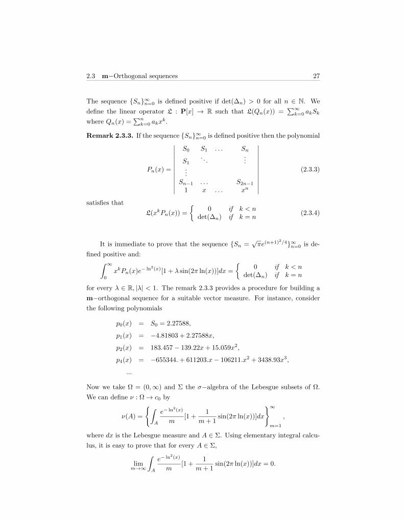
The sequence Sn∞n=0 is defined positive if det(∆n) > 0 for all n ∈ N. We
define the linear operator L : P[x] → R such that L(Qn(x)) =∑∞k=0 akSk
where Qn(x) =∑nk=0 akx
k.
Remark 2.3.3. If the sequence Sn∞n=0 is defined positive then the polynomial
Pn(x) =
∣∣∣∣∣∣∣∣∣∣∣∣
S0 S1 . . . Sn
S1. . .
......
Sn−1 . . . S2n−1
1 x . . . xn
∣∣∣∣∣∣∣∣∣∣∣∣(2.3.3)
satisfies that
L(xkPn(x)) =
0 if k < n
det(∆n) if k = n(2.3.4)
It is immediate to prove that the sequence Sn =√πe(n+1)2/4∞n=0 is de-
fined positive and:∫ ∞0
xkPn(x)e− ln2(x)[1 + λ sin(2π ln(x))]dx =
0 if k < n
det(∆n) if k = n
for every λ ∈ R, |λ| < 1. The remark 2.3.3 provides a procedure for building a
m−orthogonal sequence for a suitable vector measure. For instance, consider
the following polynomials
p0(x) = S0 = 2.27588,
p1(x) = −4.81803 + 2.27588x,
p2(x) = 183.457− 139.22x+ 15.059x2,
p4(x) = −655344.+ 611203.x− 106211.x2 + 3438.93x3,
...
Now we take Ω = (0,∞) and Σ the σ−algebra of the Lebesgue subsets of Ω.
We can define ν : Ω→ c0 by
ν(A) =
∫A
e− ln2(x)
m[1 +
1
m+ 1sin(2π ln(x))]dx
∞m=1
,
where dx is the Lebesgue measure and A ∈ Σ. Using elementary integral calcu-
lus, it is easy to prove that for every A ∈ Σ,
limm→∞
∫A
e− ln2(x)
m[1 +
1
m+ 1sin(2π ln(x))]dx = 0.

28 Chapter 2. m−Orthogonal sequences with respect to a vector measure
This shows that ν is well defined and so countably additive. Moreover, it is also
clear that the functions pl(x) ∈ L2(m) and they satisfy that for all j < l,∫ ∞0
pj(x)pl(x)dν = Blδjl
where Bl is a non null constant for all l ∈ N.
Example 2.3.4. Let us provide another example of ν-orthogonal sequence with
respect to a vector measure ν. Consider the family Pn,k∞n,k of Stieltjes-Wigert
polynomials. For every n ∈ N and k ∈ N,
Pn,k(x) =(−1)nq(k)n/2+1/4√∏k
j=1(1− q(k)j)
n∑i=0
[(n
i
)]q
q(k)(i2)(−√q(k)x)i
where q(k) = exp(−(2k2)−1), k is a positive integer and we call[(n
i
)]q
=(1− q(k)n)(1− q(k)n−1) · · · (1− q(k)n−i+1)
(1− q(k))(1− q(k)2) · · · (1− q(k)i),
as a q-binomial coefficient also called a Gaussian coefficient or Gaussian poly-
nomial. Let us also consider the family of normalized weights wk∞k=1 =
1α(k)√πkx−k
2 log x∞k=1 in [0,∞), where α(k) = e1
4k2 . It is well-known that
the family of polynomials above is orthogonal in the following sense: for a fixed
k ∈ N, the sequence Pn,k∞n=1 is orthogonal with respect to the weight wk, i.e.∫ ∞0
Pn,k(x)Pm,k(x)wk(x)dµ(x) = 0, n 6= m,
see [63, 2.7]. Consider the Lebesgue measure space ([0,∞),B, µ) and take the
set Ω0 =⋃∞k=1([0,∞)× k). Let us define the σ-algebra Σ0 given by elements
of the form A =⋃∞k=1(Ak × k) ⊆ Ω0, where Ak is a Lebesgue measurable
subset of [0,∞) for every k. Let us define the vector measure ν : Σ0 → c0 as
ν(A) :=
∞∑k=1
(1
k
∫Ak
wk(x)dµ(x))ek,
where A is an element of Σ0 as above.
Suppose now that the polynomials Pn,k are normalized in the Hilbert space
L2([0,∞), wkdµ) given by the weighted measure wk(x)dµ(x). Define the func-
tions Qn,k : Ω0 → [0,∞) by
Qn,k((xj , j)) := k1/2 Pn,k(xj) δk,j ,

2.3 m−Orthogonal sequences 29
for (xj , j) ∈ Ω0. A careful writing of the integrals with respect to ν of the
products of such functions shows that∫Ω0
Qn,kQm,sdν = 0
whenever n 6= m or k 6= s. To see this, just take into account that if k 6= s, then∫Ω0
Qn,kQm,sdν =( ∑j 6=s,k
(s1/2k1/2
j
∫ ∞0
0 · 0wj(x)dµ(x))ej
)
+(s1/2k1/2
k
∫ ∞0
Pn,k(x) · 0wk(x)dµ(x))ek
+(s1/2k1/2
s
∫ ∞0
0 · Pm,s(x)ws(x)dµ(x))es = 0
and for k = s and n 6= m,∫Ω0
Qn,kQm,kdν =(∑j 6=k
(kj
∫ ∞0
0 · 0wj(x)dµ(x))ej
)
+( ∫ ∞
0
Pn,k(x) · Pm,k(x)wk(x)dµ(x))ek = 0.
Therefore, every subsequence of Qn,k∞n,k=1 defines a ν-orthonormal sequence.
Now we are going to provide some results on the existence of m−orthonormal
sequences in L2(m). It is easy to prove the existence of m-orthonormal se-
quences of functions in any (non trivial) space of square integrable functions
with respect to a vector measure.
Lemma 2.3.5. Suppose that there is a sequence An∞n=1 into Σ of disjoint
non ‖m‖−null sets. Then there is a m-orthonormal sequence in L2(m).
Proof. The characteristic functions χAn ∈ L2(m), for every n ∈ N. Moreover,
since ‖m‖(A) 6= 0, there is a subset Bn ⊂ A such that ‖m(Bn)‖X > 0. Let us
define fn =χBn
‖m(Bn)‖1/2 , n ∈ N. Then∫f2ndm =
∫χ2Bn
‖m(Bn)‖dm =
1
‖m(Bn)‖
∫χBndm =
m(Bn)
‖m(Bn)‖6= 0.
On the other hand, if n 6= k for n, k ∈ N, it is clear that∫fnfkdm = 0,
since Bn ∩Bk = ∅, and the result is obtained.

30 Chapter 2. m−Orthogonal sequences with respect to a vector measure
It is clear that an m-orthonormal sequence also is also orthogonal for each
associated m-positive measure 〈m, x′〉. The notion of m-orthonormal sequence
is the natural generalization of the concept of orthonormal sequence in a Hilbert
space L2(µ) and has been studied in [48, 59]. As the reader will see, the results on
almost everywhere convergence that will be shown in next chapter prove the ones
that hold for the case of series in Hilbert spaces. However, the m-orthonormality
requirement for a sequence of functions in the non scalar case introduces a strong
restriction, in particular regarding completeness of the orthogonal sequence. An
orthonormal set Ψ is said to be complete if there exists no other orthonormal
set containing Ψ, that is, Ψ must be a maximal orthonormal set. It is easy
to prove that an orthonormal set Ψ is complete if and only if for any f such
that f is orthogonal to Ψ, f must be zero. Let us show this fact with an easy
construction. Suppose that (Ω0,Σ0, µ0) is a probability measure space, and
consider a complete orthonormal sequence gi∞i=1 in L2(µ0) such that g1 =
χΩ0 . Suppose that gi∞i=1 is also m0-orthonormal sequence for a countably
additive measure m0 : Σ0 → X that is absolutely continuous with respect to
µ0. Then every measure (m0)x′ , x′ ∈ X ′, is µ0-continuous, and there is a
function hx′ ∈ L1(µ0) such that d(m0)x′ = hx′dµ0. For every k ≥ 2,
0 = 〈∫g1gkdm0, x
′〉 =
∫gkhx′dµ0.
If moreover hx′ ∈ L2(µ0), since the sequence gi∞i=1 is complete, the equalities
above imply hx′ = r(x′)χΩ0for a real number r(x′). Therefore, if we assume
that for every x′ ∈ X ′ the corresponding Radon-Nikodym derivative belongs to
L2(µ0), we obtain that
(m0)x′(A) = r(x′)µ0(A), A ∈ Σ0, x′ ∈ X ′.
This relation establishes a strong restriction on m0. For instance, suppose that
X is a Banach space with an unconditional basis ei∞i=1. Then m0(A) =∑∞i=1〈m0(A), e′i〉ei, where e′i∞i=1 are the corresponding biorthogonal function-
als and A ∈ Σ0. In this case the relation above implies that
m0(A) = (
∞∑i=1
r(e′i)ei)µ0(A)
for every A ∈ Σ0, i.e. m0 can be in fact considered as a scalar positive measure.
Remark 2.3.6. The above argument shows that in general we cannot expect
completeness for m-orthonormal sequence of functions, although under certain

2.4 Strongly m−orthogonality 31
(strong) assumptions it is possible to obtain m-orthonormal basis for L2(m)
(see [48]). Thus, although the results that we present in what follows can be
used to obtain information about standard orthonormal sequences fi∞i=1 in
Hilbert spaces L2(µ), the procedure of splitting the scalar measure µ into a
vector measure m preserving orthonormality is essentially limited by a certain
non completeness assumption for fi∞i=1.
The next result is a direct consequence of the Kadec and Pelczynski pro-
cess for obtaining disjoint sequences -see Chapter 1.3 for notation-. It provides
a method for, given a convenient sequence fnn, finding a disjoint (and then
m−orthogonal) subsequence of fnn.
Corollary 2.3.7. Let H be Hilbert space which is also a Banach lattice and
m : Σ → H a positive vector measure such that ‖m‖(Ω) = 1. Take a Rybakov
control measure µ = |x′0m| for m with ‖x′0‖ = 1. If fnn ⊂ L2(m) is such that
‖fn‖L2(m) = 1 for all n and fnn * ML2(m)(ε) for all ε > 0 then there exists
a subsequence hk∞k=1 ⊂ L2(m) such that |hk| ≤ |fnk | for all k and hk∞k=1
is a m−orthogonal sequence in L2(m). Moreover, fnk∞k=1 and hk∞k=1 are
equivalent unconditional basic sequences that satisfies limk→∞ ‖fnk−hk‖L2(m) =
0.
The proof is a direct application of Theorem 1.3.3. Note that limk→∞ ‖fnk−hk‖L2(m) = 0 and ‖fnk‖L2(m) = 1 for all k implies that
∫h2kdm 6= 0 for large
enough k.
2.4 Strongly m−orthogonality
In this section we present the last notion of orthogonality, that is the most
restrictive. In what follows we will establish the conditions that are required in
order to construct a strongly m−orthonormal system.
Definition 2.4.1. Let us consider a separable Hilbert space H with an or-
thonormal sequence ei∞i=1 and a countably additive vector measure m : Σ →H. We say that fi∞i=1 ⊂ L2(m) is a strongly m-orthogonal sequence if∫fifjdm = δijeiki, ki > 0. If ki = 1 for every i, we say that it is a strongly
m-orthonormal sequence.

32 Chapter 2. m−Orthogonal sequences with respect to a vector measure
It is clear that if fnn is a strongly m-orthogonal sequence then fnn is
a m-orthogonal sequence and therefore, in the case when H is also a Banach
lattice and m is positive, fnn is weak m-orthogonal. The converse is not true.
Example 2.4.2. Let rk(x) = sgn[sin(2k−1x)] be the Rademacher function of
period 2π, defined at the interval Ek = [2(k − 1)π, 2kπ], k ∈ N. We define the
following countably additive vector measure,
m(A) :=
∞∑k=1
(−1)
2k
(∫A∩Ek
rkdµ
)ek ∈ `2.
Note that if f ∈ L1(m) then∫fdm = (− 1
2k
∫Ekfrkdµ)k ∈ `2. We consider the
next sequence of functions
f1(x) = sinx · χ[π,2π]
f2(x) = sin 2x · (χ[0,2π] + χ[ 72π,4π])
f3(x) = sin 4x · (χ[0,4π] + χ[ 234 π,6π])
...
fk(x) = sin 2k−1x · (χ[0,2(k−1)π] + χ[(2k− 1
2k−1 )π,2kπ]), k ≥ 2.
These family of functions of L2(m) can be used to define a strongly m−orthogonal
Figure 2.1: Functions f1(x), f2(x) and f3(x).
sequence (see figure 2.1), since⟨∫f2ndm, en
⟩= − 1
2n
∫En
f2nrndµ =
π
22n⟨∫f2ndm, ek
⟩= − 1
2k
∫Ek
f2nrkdµ = 0, ∀k 6= n⟨∫
fnfmdm, ek
⟩= − 1
2k
∫Ek
fnfmrkdµ = 0, for n 6= m and ∀k

2.4 Strongly m−orthogonality 33
If we define
Fn(x) =2n√πfn(x),
we obtain∫F 2i dm = ei, ∀i ∈ N and
∫FiFjdm = 0, ∀i, j ∈ N, i 6= j.
Now we adapt a well know result of Bessaga and Pelczynski (see for in-
stance [24], Ch.V) to the context of sequences of functions on spaces of integrable
functions with respect to a vector measure in the following sense. We want to
identify when a sequence∫
f2ndm
∞n=1⊂ H is a basic sequence of H. This will
be the main tool for obtaining what we have denoted strongly m−orthogonal
sequences. The first requirement in Corollary 2.4.3 is obviously satisfied in the
case of m-orthonormal sequences. The second condition constitutes the key of
the problem.
Corollary 2.4.3. Let m : Σ −→ H be a vector measure, and consider the
basis en∞n=1 of H. Let fn∞n=1 be a sequence in L2(m). If the sequence∫f2ndm
∞n=1
satisfies
(1) infn∥∥∫ f2
ndm∥∥H
= ε > 0, and
(2) limn
⟨ek,∫f2ndm
⟩= 0, k ∈ N,
then∫
f2ndm
∞n=1
has a subsequence which is a basic sequence, moreover it is
equivalent to a block basic sequence of en∞n=1 .
The proof of this corollary is an immediate consequence of Theorem 3 [7].
Let us highlight with an example the geometrical meaning of this condition by
showing a particular sequence of functions that satisfies Remark 1.2.5. This is
in a sense the canonical situation, involving disjointness.
Example 2.4.4. Let (Ω,Σ, µ) be a probability measure space. Let us consider
the following vector measure m : Σ→ `2,
m(A) :=
∞∑i=1
µ(A ∩Ai)ei ∈ `2, A ∈ Σ,
where Ai∞i=1 is a disjoint measurable partition of Ω, with µ(Ai) 6= 0 for all i ∈N. Notice that
∫f2dm =
∑∞i=1(
∫Aif2dµ)ei ∈ `2 for all f ∈ L2(m). Consider

34 Chapter 2. m−Orthogonal sequences with respect to a vector measure
the sequence of functions fn∞n=1 in L2(m), defined by fn := χAn/(µ(An))1/2.
For every k ∈ N, the following holds:
limn
⟨ek,
∫f2ndm
⟩= lim
n
⟨ek,
∞∑i=1
(∫Ai
f2ndµ
)ei
⟩= lim
n
∫Ak
f2ndµ = 0.
‖∫f2ndm‖`2 = 1 for all n.
Therefore, condition (2) of Corollary 2.4.3 is fulfilled in this example: the
role of disjointness is clear. The geometrical meaning of this condition by show-
ing a particular sequence of functions that satisfies Remark 1.2.5. This is in a
sense the canonical situation, involving disjointness.
For the case of vector measures m having a compact integration operator,
we provide an easy argument showing that there are no strong m−orthogonal
sequences in L2(m) (see Proposition 3.48 [49]). In particular, this shows that the
existence of such sequences is a pure vector measure phenomenon. In fact, this
property is closely related to the existence of strongly m-orthonormal sequences.
Compactness of the integration map is nowadays well characterized. It is a very
strong property in the sense that it implies that the space L1(m) is isomorphic
to an L1 space of an scalar measure. The result can be found in Proposition
3.48. [49] (see also the references there in). The following necessary condition
for the compactness of the integration operator shows this.
Lemma 2.4.5. Let m : Σ −→ H be an countably additive vector measure. If
there exists a strongly m-orthonormal sequence in L2(m), then the integration
operator Im : L1(m) −→ H is not compact.
Proof. Let us consider an orthonormal sequence eii in H and let fii be a
strongly m−orthogonal sequence in L2(m). Then∫fifjdm = δijei, an thus∫
f2i dm = ei = Im(f2
i ).
Thereforef2i
∞i=1⊂ BL1(m) and so the sequenceIm(f2
i )∞i=1⊂ Im(BL1(m)) ⊂ Im(BL1(m))
does not admit any convergent sub-sequence, from what follows that Im(BL1(m))
is not compact and so, Im(BL1(m)) is not relatively compact, what allows us to
conclude that Im is not compact.

2.4 Strongly m−orthogonality 35
Therefore, if Im : L1(m) −→ H is compact then no strongly m-orthonormal
sequence exists in L2(m).
The following theorem gives a necessary condition -and, in a sense, also
a sufficient condition- for the existence of strongly orthonormal sequences in a
space of functions L2(m) starting from a given m-orthonormal sequence. In
general, it is not possible to find a subsequence satisfying this condition. How-
ever, as the reader will see, it is possible to find a vector measure m∗ satisfying
that L2(m) = L2(m∗) and with respect to which there is a subsequence that
is strongly m∗-orthonormal. We need first the following lemma, which proof is
elementary.
Lemma 2.4.6. Let m : Σ → `2 be a vector measure. Let ϕ : `2 → H be
an isomorphism, where H is a separable Hilbert space, and consider the vector
measure m∗ = ϕ m. Then the spaces L2(m) and L2(m∗) are isomorphic, and
for every f ∈ L2(m),∫f2dm∗ = ϕ(
∫f2dm).
We need the following formal requirement for the elements of the sequence
fn∞n=1 in the result below. We say that a function f ∈ L2(m) is normed by
the integral if ‖f‖L2(m) = ‖∫f2 dm‖1/2. This happens for instance when the
vector measure is positive —i.e. it has its range in the positive cone of a Banach
lattice—, see [23] or [49, Lemma 3.13]. We impose this condition for the aim
of clarity, although the result could be adapted using a convenient renorming
process in order to avoid this requirement.
Theorem 2.4.7. Let us consider a vector measure m : Σ → `2 and an m-
orthonormal sequence fn∞n=1 of functions in L2(m) that are normed by the
integrals. Let en∞n=1 be the canonical basis of `2. If
limn
⟨ek,
∫f2ndm
⟩= 0
for every k ∈ N, then there exists a subsequence fnk∞k=1 of fn∞n=1 and a
Hilbert space valued measure m∗ : Σ → H such that fnk∞k=1 is a strongly
m∗-orthonormal. Moreover, m∗ can be chosen as m∗ = φm for some Banach
space isomorphism φ from `2 onto H.
Proof. Consider an m-orthonormal sequence fn∞n=1 in L2(m) and the se-
quence of integrals∫
f2ndm
∞n=1
. As an application of Corollary 2.4.3, we
36 Chapter 2. m−Orthogonal sequences with respect to a vector measure
get a subsequence∫
f2nkdm∞k=1
that is equivalent to a block basic sequence
e′nk∞k=1 of the canonical basis of H. Recall that following the notation given
in the Preliminaries αi,j are the constants that appear in the definition of the
block basic sequence. Associated to the block basic sequence obtained there is
an isomorphism ϕ
A := span(e′nk)H ϕ−→ B := span
(∫f2nkdm
)`2such that ϕ(e′nk) :=
∫f2nkdm, k ∈ N.
We can suppose without loss of generality that the elements of the sequence
e′nk∞k=1 have norm one. To see this, it is enough to consider the following in-
equalities. First note that there are positive constants k and K such that for
every n ∈ N, k = k‖∫f2nkdm‖ ≤ ‖e′nk‖ ≤ K‖
∫f2nkdm‖ = K as a conse-
quence of the existence of the isomorphism ϕ. Let λi∞i=1 be a sequence of real
numbers. Then
‖∞∑i=1
λie′i‖e′i‖‖22 =
∞∑i=1
|λi|2(∑qij=pi|αi,j |2)
‖e′i‖2=
∞∑i=1
qi∑j=pi
|λi|2|αi,j |2
‖e′i‖2.
The existence of an upper and a lower bound for the real numbers ‖e′i‖ given
above provides the equivalence between this quantity and
‖∞∑i=1
λie′i‖22
for every sequence of real numbers λi∞i=1.
Since each closed subspace of a Hilbert space is complemented, there is a
subspace Bc such that
`2 = B ⊕2 Bc
isometrically, where this direct sum space is considered as a Hilbert space (with
the adequate Hilbert space norm). We write PB and PBc for the corresponding
projections. Let us consider the linear map φ := ϕ−1⊕ Id, where Id : Bc → Bc
is the identity map.
B ⊕2 Bc φ−→ A⊕2 B
c.
Note that H := A⊕2 Bc is a Hilbert space when the scalar product
〈x+ y, x′ + y′〉H = 〈x, x′〉H + 〈y, y′〉H , x+ y, x′ + y′ ∈ A⊕2 Bc

2.4 Strongly m−orthogonality 37
is considered. Obviously, φ is an isomorphism. Let us consider also the vector
measure m∗ := φ m,
Σm−→ `2
φ−→ A⊕2 Bc.
By Lemma 2.4.6, L2(m) = L2(φ m) = L2(m∗). Let us show that fnk∞k=1
is a strongly m∗-orthonormal sequence. We consider the orthonormal sequence
(e′nk , 0)∞k=1 in H. The first condition in the definition of strongly orthonormal
sequence is fulfilled, since∫f2nkdm∗ =
∫f2nkd(φ m) = φ
(PB(
∫f2nkdm), PBc(
∫f2nkdm)
)
=
(ϕ−1(
∫f2nkdm), 0
)= (e′nk , 0)
for every k ∈ N. The second one is given by the following calculations. For
k 6= l,∥∥∥∥∫ fnkfnldm∗∥∥∥∥ =
∥∥∥∥∫ fnkfnld(φ m)
∥∥∥∥ =
∥∥∥∥φ(
∫fnkfnldm)
∥∥∥∥ = ‖φ(0)‖ = 0,
since φ is continuous and fnk∞k=1 is a m-orthonormal sequence. Thus∫fnkfnldm
∗ = 0.
This proof the theorem.
Corollary 2.4.8. Let m :∑−→ Υ (Υ a separable Hilbert space) and let
fn∞n=1 be an m-orthonormal sequence in L2(m), such that∫
Ωf2ndm
∞n=1
is
weakly null in H. Then there is a subsequence fnk∞k=1 and a complete or-
thonormal basis nj∞j=1 for Υ, such that fn(k)∞k=1 is strongly m-orthonormal
with the basis nj∞j=1.
Remark 2.4.9. In a certain sense, the converse of the theorem above also holds.
Take as the vector measure m∗ the measure m itself with values in `2 and
consider the canonical basis en∞n=1. Clearly, every strongly m-orthonormal
sequence is m-orthonormal and satisfies the condition limn
⟨ek,∫f2ndm
∗⟩ = 0,
since ⟨ek,
∫f2ndm
∗⟩
= 〈ek, en〉 = 0, k 6= n.

Chapter 3
The Menchoff-RademacherTheorem for L2(m)
One of the key issues that arose in the late XIX, it is when the development of a
Fourier series of a continuous function converges pointwise to the function. The
first result that answered partially this question was given by Dirichlet showing
that if a function has bounded variation then its Fourier series converges point-
wise everywhere to the local average of the function. If we change the summation
method we can obtain the convergence almost everywhere. Later Fejer showed
that if we consider the sums of Cesaro sums instead of the ordinary sums then
the Fourier series of a continuous function converges pointwise everywhere to the
function. Luzin conjectured that the Fourier series of a Lebesgue-measurable
function of L2 converges almost everywhere. Kolmogorov showed an example
of a function in L1 whose Fourier series diverges almost everywhere. Finally
Carleson proved the conjecture of Luzin in 1966. In this section we analyze
almost everywhere convergence of weak m-orthogonal sequences, and we obtain
a version of a Mechoff-Rademacher Theorem.
Let (Ω,Σ, µ) be a finite measure space, and consider an orthonormal se-
quence fii of real functions in L2(µ) and a sequence of real numbers aii. The
Menchoff-Rademacher Theorem (see [45, 46, 51]) is the main result concerning
39
40 Chapter 3. The Menchoff-Rademacher Theorem for L2(m)
µ-almost everywhere convergence of the norm convergent series∑∞i=1 aifi, and
establishes that it converges µ-a.e. if∑∞i=1 |ai|2log2(i + 1) < ∞. Although for
particular (even complete) orthonormal sequences this result can be improved
(for instance, it is enough that∑∞i=1 |ai|2 < ∞ for the Haar and the trigono-
metric sequences, see 1.6.1 in [1] and [11]), it is optimal if we consider any
orthonormal sequence.
In this chapter we prove a Menchoff-Rademacher type theorem on almost
everywhere convergence of series in L2(m) and we analyze some particular
cases regarding c0-sums of Lebesgue spaces. Although several properties and
applications of orthogonal series with respect to a vector measure are known
([35, 36, 48]), the question of the almost everywhere convergence of series de-
fined by such functions has not been studied yet. Following this research and
as an application of the criterion for weak orthogonality, the results that we
present provide also reasonable answers to the problems concerning almost ev-
erywhere convergence of (strongly orthogonal) series that appear in [48, 59].
From the methodological point of view, we follow the technique that is used in
[64] to study the almost everywhere convergence of series. In Section III.H of
this book it is shown that there exists a deep link between the evaluation of
2-summing norms for a special class of operators between sequence spaces and
the problems concerning almost everywhere convergence of series; the origin of
this idea can be already found in [6, Section 4] (see also [50]). Recently, related
techniques have been used in [14, 20, 21], for instance for proving generaliza-
tions of the Menchoff-Rademacher Theorem for vector valued Banach function
spaces ([21]). We explain the required version of this argument for our work
in the proof of Theorem 3.2.2 and we establish the requirements for obtain-
ing the almost everywhere convergence of series defined by weak orthogonal
sequences. Finally, we provide a technique to construct non trivial examples of
weak m-orthogonal sequences fi∞i=0 in particular Banach lattices such that
the requirement∑∞i=1 a
2i <∞ on the sequence of scalar coefficients implies the
a.e. convergence of the series∑∞i=1 aifi.
3.1 About almost everywhere convergence of sequences in L2(m) 41
3.1 About almost everywhere convergence of se-quences in L2(m)
Let (Ω,Σ) be a measureble space, X a Banach lattice and m : Σ→ X a vector
measure. Let us establish first some general results on m−a.e. convergence
of sequences in L2(m). Throughout this section fnn will be a sequence of
measurable functions of integrable square with respect to a vector measure m.
Definition 3.1.1. Given a function f ∈ L2(m), we define the set
En(α) = ω ∈ Ω :| fn(ω)− f(ω) |≥ α. (3.1.1)
The sequence fn∞n=1 is said to convergence in vector measure m to f if
limn→∞
‖m ‖ (En(α)) = 0 (3.1.2)
for each α. Since m is a positive vector measure, the condition (3.1.2) is equiv-
alent to the following expression
limn→∞
‖m(En(α)) ‖X= 0.
The following two results can be found in Section 7 [5] for scalar measures.
Lemma 3.1.2. Let fn∞n=1 be a sequence of measurable real-valued functions
which converge to a measurable function f in L2(m), then fn∞n=1 converges
to f in vector measure m.
Proof. Since the inequalities
‖fn−f‖L2(m) ≥ ‖(fn−f)χEn(α)‖L2(m) ≥ ‖αχEn(α)‖L2(m) = |α|‖m‖(En(α)
)1/2.
hold for any constant K and it is clear that if fn → f in L2(m) then the last
term converges to 0.
The above result can be obtained immediately if we apply the following
implications. Let µ be a Rybakov measure. Then
• fn → f in vector measure m if and only if fn → f in µ measure.
• If fn → f in L2(m) then fn → f in L2(µ).

42 Chapter 3. The Menchoff-Rademacher Theorem for L2(m)
Definition 3.1.3. The sequence fn∞n=1 of measurable real-valued functions
converges m-almost everywhere to a measurable function f if there exists a set
M in Ω with ‖m‖(M) = 0, such that for every ε > 0 and ω ∈ Ω−M there exists
a natural number N(ε, ω) such that if n ≥ N(ε, ω) then | fn(ω)− f(ω) |< ε.
Proposition 3.1.4. Let fn∞n=1 be a sequence of real-valued measurable func-
tions such that converges to a measurable function f in the norm of L2(m).
Then there is a subsequence which converges m-almost everywhere to f .
Proof. By Lemma 3.1.6 we have that if fn∞n=1 converge to a measurable
function f in the norm of L2(m) then fn∞n=1 converges to f in vector measure
m. Now we proof that there exists a subsequence that converges m-almost
everywhere to f . Select a subsequence fnk of fn such that the set
Ek = ω ∈ Ω :| fnk(ω)− f(ω) |≥ 2−k
satisfies ‖m‖(Ek) < 2−k. Let Fk =⋃∞j=k Ej so that Fk ∈ Σ then
‖m‖(Fk) = ‖m‖(∞⋃j=k
Ej) ≤∞∑j=k
‖m‖(Ej) ≤∞∑j=k
2−j = 2−(k−1).
If i ≥ k and ω is not into Fk then |fni(ω) − f(ω)| ≤ 2−k. Let F =⋂∞k=1 Fk.
Then ‖m‖(F ) = 0. From the argument just given it follows that fnk converges
m-almost everywhere to the measurable real-valued function f .
In what follows we analyze some properties of the integrals in the subspaces
generated by m−orthogonal sequences.
Lemma 3.1.5. Let fi∞i=1 be an m−orthonormal sequence. For all I0 ⊂ N and
(λi)i∈I0 ⊂ R such that g =∑i∈I0 λifi converges in L2(m), then
∫gfjdm = 0
if j ∈ N\I0
Proposition 3.1.6. Let Y (ν) be a Banach function space, m : Σ → Y (ν) a
positive vector measure and fi∞i=1 a m−orthogonal sequence and let f0 be a
measurable function such that f0 ∈ L2(m). Then if ‖ f0 −∑ni=1 λifi ‖L2(m)
converges to 0 we have:
(1)∫
(∑ni=1 λ
2i f
2i )dm is an increasing positive sequence that converges to∫
f20 dm in norm and so ν−almost everywhere.

3.1 About almost everywhere convergence of sequences in L2(m) 43
(2)∫
(∑ni=1 λifi − f0)2dm is a decreasing positive sequence that converges 0
in norm and so ν−almost everywhere.
(3)∫ ∑n
i=1 λifidm converges to∫f0dm ν−almost everywhere.
Proof. We suppose that ‖ f0 −∑ni=1 λifi ‖L2(m) converges to 0. Then∫
|n∑i=1
λifi − f0 |2 dm =
∫(
n∑i=1
λifi − f0)2dm
=
n∑i=1
∫λ2i f
2i dm +
∫f2
0 dm− 2n∑i=1
λi
∫fif0dm
=
n∑i=1
∫λ2i f
2i dm +
∫f2
0 dm
−2
n∑i=1
λi
∫fi(
n∑k=1
λkfk)dm− 2
n∑i=1
λi
∫fi(
∞∑k=n+1
λkfk)dm
=
n∑i=1
∫λ2i f
2i dm +
∫f2
0 dm− 2
n∑i=1
∫λ2i f
2i dm
=
∫f2
0 dm−n∑i=1
λ2i
∫f2i dm.
Hence, we have that∑n
i=1 λ2i
∫f2i dm
n
is an increasing sequence that con-
verges to∫f2
0 dm in norm and so ν−almost everywhere, and also we have that
(2) holds. In order to prove (3), recall that if T : X(ν)→ Y (ν) is a positive op-
erator between Banach function spaces, we always have that if 0 ≤ f, g ∈ X(µ),
f · g ∈ X(µ) then T (f · g) ≤ T (f2)1/2 · T (g2)1/2. Since the integration operator
with respect to m is positive, just consider the (pointwise) inequalities
(
∫(f0 −
n∑i=1
λifi)2dm)
12 (m(Ω))
12 ≥|
∫(f0 −
n∑i=1
λifi)dm |
=|∫f0dm−
∫(
n∑i=1
λifi)dm |
so the sequence∫ ∑n
i=1 λifidmn
converges ν−almost everywhere to∫f0dm.
Remark 3.1.7. Let Y (ν) be a Banach function space, m : Σ→ Y (ν) a vector
measure and and fi∞i=1 a m−orthogonal sequence and let f0 be a measurable
function such that f0 ∈ L2(m). If we consider an m−orthogonal subsequence
fikk of fii such that ‖ f0 −∑ni=1 λifik ‖L2(m) converges to 0 then the
Proposition 3.1.6 holds.
44 Chapter 3. The Menchoff-Rademacher Theorem for L2(m)
3.2 The Menchoff-Rademacher Theorem forweak m-orthogonal sequences
In this section we study the almost everywhere convergence of functional series
defined by (real valued) functions that are weak m-orthogonal for a vector
measure m. The vector measure is supposed to be positive through all the
chapter. We develop a technique for generalizing the arguments that prove the
Menchoff-Rademacher Theorem to our setting (see [64, III.H.22] for the scalar
measure case). It provides the adequate elements for proving more specialized
versions of this theorem depending on the properties of the space where the
vector measure is defined. Let m : Σ → X be a positive vector measure over
(Ω,Σ). Our aim is to obtain conditions on a weak m-orthogonal sequence
fii and a sequence of real numbers aii to assure 〈m, x′〉-almost everywhere
convergence of the series∑∞i=1 aifi for a certain x′ ∈ (X ′)+
m.
Let x′ ∈ (X ′)+m. Let fii be a sequence that is orthogonal with respect to
〈m, x′〉. Consider Banach sequence space L over the standard measure space on
N with canonical (normalized) basis eii. If s is a natural number, we write
Φs for the function Φs : Ω→ L given by the formula
Φs(ω) :=
s∑i=1
fi(ω)ei, ω ∈ Ω.
Note that this function belongs to the Bochner space L2(〈m, x′〉, L) for every
x′ ∈ (X ′)+m, since fi ∈ L2(m) for every i ∈ N can be considered as a (class of)
function(s) of L2(〈m, x′〉).
Definition 3.2.1. Consider a Banach sequence space L and a sequence of real
numbers a := aii. We denote by σa,L the operator σa,L : L→ `∞ given by
σa,L((λi)i) :=
(
n∑i=1
aiλi)
∞n=1
, λii ∈ L,
if it is well defined and continuous. We also write σNa,L for the operator σNa,L :
L→ `∞ defined as σa(N),L, where a(N)i = ai for every i ≥ N , and 0 otherwise.
Theorem 3.2.2. Let x′ ∈ BX′ ∩ (X ′)+m. Consider a sequence of real numbers
a = ai∞i=1 and a sequence fi∞i=1 ∈ L2(m) that is orthogonal with respect to
3.2 The Menchoff-Rademacher Theorem forweak m-orthogonal sequences 45
〈m, x′〉. Let L be a 2-concave sequence space and let M be a sequence space such
that (L′)[2] = M ′. Suppose that
(1) there is a constant K such that ‖〈∫f2i dm, x′〉si=1‖M < K for every s ∈ N
and
(2) the operators σNa,L : L→ `∞ are 2-summing and limN→∞ π2(σNa,L) = 0.
Then the series∑∞i=1 aifi converges 〈m, x′〉-a.e.
Proof. First we prove the following claim: Let Y be a Banach space and let
T : L→ Y be a 2-summing operator, then for every natural number s,
‖TΦs‖L2(〈m,x′ 〉,Y ) ≤ π2(T )‖〈∫f2i dm, x
′〉si=1‖
12
M .
To prove this, first note that the elements of the space (L′)[2] are sequences
τ = τii that satisfy that there is a sequence z′ = z′ii ∈ L′ such that for
every i ∈ N, |z′i|2 = |τi|. Since L′ is 2-convex (see [42, Proposition 1.d.4(iii)]),
(L′)[2] is a Banach space with norm ‖τ‖(L′)[2]:= ‖τii‖(L′)[2]
= ‖(|τi|1/2)i‖2L′(recall that we assume for simplicity that the 2-concavity constant of L is 1 and
then the 2-convexity constant of L′ also equals 1; see [18] and [42, Proposition
1.d.4(iii)]). Since T is 2-summing, a direct calculation (see [64, Proposition
III.F.33,b)]) gives
‖TΦs‖2L2(〈m,x′〉,Y ) ≤ π22(T ) sup
z′∈BL′
∫|〈Φs(ω), z′〉|2d〈m, x′〉.
Since fii is orthogonal with respect to 〈m, x′〉, the inequality above can be
written as
‖TΦs‖2L2(〈m,x′〉,Y ) ≤ π22(T ) sup
z′∈BL′
s∑i=1
|z′i|2∫f2i d〈m, x′〉;
all the integrals in this expression are positive, so we also obtain
supz′∈BL′
s∑i=1
|z′i|2∫f2i d〈m, x′〉 = sup
τ∈B(L′)[2]
s∑i=1
|τi|∫f2i d〈m, x′〉
= ‖(〈∫f2i dm, x′〉)si=1‖M < K.
This gives the desired inequality and proves the claim.
Now we just need to show that the requirements for the operators σNa,Lare enough to apply an standard almost everywhere convergence criterion (see

46 Chapter 3. The Menchoff-Rademacher Theorem for L2(m)
for instance [64, III.H.22]). A direct calculation shows that for each natural
numbers N and s, consider the function gN,s : Ω→ [0,∞) defined by
gN,s(ω) =∥∥σNa,L(Φs(ω)
)∥∥∞ = max
n=N,...,s
∣∣∣ n∑i=N
aifi(ω)∣∣∣.
Applying the claim for T = σNa,L we have that
‖gN,s‖L2(〈m,x′〉) = ‖σNa,LΦs‖L2(〈m,x′〉,`∞) ≤ π2(σNa,L)K1/2.
Fixing N , the sequence g2N,ss increases to h2
N where
hN (ω) = supn≥N
∣∣∣ n∑i=N
aifi(ω)∣∣∣.
Then, the monotone convergence theorem gives∫h2Nd〈m, x′〉 = lim
s→∞
∫g2N,sd〈m, x′〉 ≤ π2
2(σNa,L)K
and so hN ∈ L2(〈m, x′〉) with ‖hN‖L2(〈m,x′〉) ≤ π2(σNa,L)K1/2. Thus, condi-
tion (2) in the statement of the theorem implies that the sequence hN∞N=1
converges to 0 in L2(〈m, x′〉), and then there is a subsequence that converges
〈m, x′〉-a.e. to 0. This clearly implies that the sequence itself converges 〈m, x′〉-a.e. to 0 since it is decreasing. Hence, for 〈m, x′〉-a.e. every ω ∈ Ω and ε > 0
there is a natural number R such that for every N ≥ R,
|N∑i=1
aifi(ω)−R−1∑i=1
aifi(ω)| ≤ supn≥R|n∑i=R
aifi(ω)| = hR(ω) < ε
and then the series∑∞i=1 aifi(ω) converges 〈m, x′〉-a.e.
Note that the almost everywhere convergence with respect to a measure
defined by a positive element x′ do not provide m-almost everywhere conver-
gence, since such measures are not in general Rybakov measures. This means
that such a measure can have more null sets in the σ-algebra Σ.
Remark 3.2.3. The requirements on L in Theorem 3.2.2 show that the problem
of the almost everywhere convergence of weak m-orthogonal series is closely
related to the calculus of estimates of 2-summing norms for the operators σNa,L :
L→ `∞ for suitable sequence spaces L. The canonical examples of such spaces
are sequence spaces that satisfy that the inclusions `1 ⊆ L ⊆ `2 are well defined

3.2 The Menchoff-Rademacher Theorem forweak m-orthogonal sequences 47
and continuous; take L = `p for 1 ≤ p ≤ 2. Then (L′)[2] = (`p′)[2] = `p
′/2. If we
consider 1 ≤ q ≤ ∞ such that 1/q = 1/p − 1/p′, then the space M satisfying
M ′ = ((`p)′)[2] is `q (c0 if p = 2). In the following section we develop the case
p = 1, for which (L′)[2] = (`∞)[2] = `∞, and then M = `1.
Let us finish this section by giving two estimates for these norms (we give
the estimates for σa,L, the ones for σNa,L are obtained with the same arguments).
Note that a direct application of the following inequalities to Theorem 3.2.2
provides formulas involving the sequence ”a” that can be directly computed.
(1) The first one comes from an application of Grothendieck´s Theorem and
can be used for the case of operators σa,`1 : `1 → `∞ that are still contin-
uous when defined as σa,`2 : `2 → `∞. Consider a sequence a ∈ `2. In this
case we can write a factorization of σa,`1 as σa,`2 id, where id : `1 → `2 is
the inclusion map. This map is 1-summing (see for instance 17.14 in [19]),
which implies that it is also 2-summing, and thus σa,`1 is so. Moreover,
π2(σa,`1) ≤ π2(id)‖σa,`2‖`1 ≤ (
∞∑i=1
a2i )
12 ,
(see e.g Exercise 11.5 in [19] for the estimate of π2(id)). Of course, the
same argument can be used for general σa,L : L → `∞ whenever it can
be factored through id : `1 → `2. This estimate gives the following result:
If fii ⊂ L2(m) is orthogonal with respect to 〈m, x′〉 for some x′ ∈BX′ ∩ (X ′)+
m and (∫f2i d〈m, x′〉)i ∈ `1, then
∑i≥1 aifi converges 〈m, x′〉-
a.e. for all aii ∈ `2.
(2) For the second one the argument is similar, but using the fact that the
operator σb,`1 is integral —we write ι(T ) for the integral norm of an op-
erator T—, where b = 1/log(i + 1)i (see the reference to the Bennet-
Maurey-Nahoum Theorem in [20, Section 4], and [19] for the definition and
properties of integral operators). Suppose that the sequence ”a” satisfies
that
‖ailog(i+ 1)i‖L′ <∞.
This requirement is the natural generalization of the Menchoff-Rademacher
condition for a.e. convergence. We can obtain the factorization through
`1 given by σa,L = σb,`1 Dc, where Dc is the diagonal operator defined
48 Chapter 3. The Menchoff-Rademacher Theorem for L2(m)
by the sequence ci = ailog(i+ 1), since
π2(σa,L) ≤ ι(σa,L) ≤ ι(σb,`1)‖Dc‖ ≤ ι(σb,`1)‖ailog(i+ 1)i‖L′ .
The same factorization can be used for every sequence b such that σb,`1
is 2-summing. This estimate gives the following result: If fii ⊂ L2(m)
is orthogonal with respect to 〈m, x′〉 for some x′ ∈ BX′ ∩ (X ′)+m and
∫f2i d〈m, x′〉i ∈ `r for 1 < r ≤ ∞, then
∑i≥1 aifi converges 〈m, x′〉-a.e.
for all aii ⊂ R such that(ai log(i+ 1)
)∈ `q for q = 2r
r−1 .
The following results combine Theorem 2.2.3, Theorem 3.2.2 and the remark
above to give several criteria for 〈m, x′〉-a.e. convergence of sequences in L2(m).
Corollary 3.2.4. Let fi∞i=1 be a sequence in L2(m). Let L be a 2-concave
sequence space and let M be a sequence space such that (L′)[2] = M ′. Let ∆ =
εii a sequence such that εisi=1 ∈ M for all s ∈ N with sups ‖εi∞i=1‖ < ∞and let a = aii be a sequence of real numbers, let BS,∆ be the convex weak*
compact subset (see 2.2.1 for definition) and suppose that
(1) the operators σNa,L : L → `∞ are 2-summing and limN→∞ π2(σNa,L) = 0
and
(2) for every finite sequence of non negative real numbers γkk such that∑k γk = 1, indexes ik, jk ∈ N, ik 6= jk, and θk ∈ −1, 1,
〈(γk), (εik + εjk)〉 ≤ ‖〈(γk), (ϕik,jk,θk)〉‖BS,∆ .
Then there is an element x′ ∈ X ′ such that the sequence
fi√εi
i
is orthonormal
in L2(〈m, x′〉) and the series∑∞i=1 aifi converges 〈m, x′〉-a.e.
The same result can be written in terms of the properties of the sequence
of the integrals.
Corollary 3.2.5. Let fi∞i=1 be a sequence in L2(m) such that ‖∫f2i dm‖si=1 ∈
M for all s ∈ N with sups ‖‖∫f2i dm‖∞i=1‖ < ∞. Let L be a 2-concave se-
quence space and let M be a sequence space such that (L′)[2] = M ′. Let a = aiibe a sequence of real numbers and suppose that
(1) the operators σNa,L : L → `∞ are 2-summing and limN→∞ π2(σNa,L) = 0
and

3.2 The Menchoff-Rademacher Theorem forweak m-orthogonal sequences 49
(2) there exists ∆ = εii such for every finite sequence of non negative real
numbers γkk such that∑k γk = 1, indexes ik, jk ∈ N, ik 6= jk, and
θk ∈ −1, 1,
〈(γk), (εik + εjk)〉 ≤ ‖〈(γk), (ϕik,jk,θk)〉‖BS,∆ .
Then there is an element x′ ∈ X ′ such that the sequence
fi√εi
i
is orthonormal
in L2(〈m, x′〉) and the series∑∞i=1 aifi converges 〈m, x′〉-a.e.
Example 3.2.6. (1) For the case of `1-valued measures and L = `2, we ob-
tain using Remark 2.2.4 that the result is similar to the one that holds
for scalar measures. Let m : Σ → `1 be a positive vector measure and
consider a sequence fii ⊆ L2(m) of norm one functions. Let a = aiibe a sequence of real numbers and suppose that
(a) the operators σNa,`2 : `2 → `∞ are 2-summing and limN→∞ π2(σNa,`2) =
0, and
(b)√
2 ≤ ‖fi + θfj‖L2(m) for all i, j ∈ N, i 6= j, and θ ∈ −1, 1.
Then Corollary 3.2.5 gives an element x′ ∈ `∞ such that the sequence fiiis orthonormal in L2(〈m, x′〉) and the series
∑∞i=1 aifi converges 〈m, x′〉-
a.e. For example, a direct calculation shows that for x′ = (1, 1, 1, ...), the
result holds.
(2) Let us show an application regarding Example 2.2.5 also for L = `2.
Let eii be the canonical basic sequence in `∞ and take an `∞ valued
(countably additive) positive vector measure ν, a sequence of functions
fii ∈ L2(m) such that∫f2i d〈ν, ej〉 = 1 for every i, j ∈ N and a sequence
a = aii such that the operators σNa,`2 : `2 → `∞ are 2-summing with
limN→∞ π2(σNa,`2) = 0. Assume also that for every finite sequence of non
negative real numbers γkk such that∑k γk = 1, indexes ik, jk ∈ N,
ik 6= jk, and θk ∈ −1, 1,
2 ≤ supi
∣∣ ∫ ∑k
γk(fik + θkfjk)2d〈ν, ei〉∣∣.
Then by Corollary 3.2.5 there is an element x′ ∈ (`∞)′ such that the se-
quence fii is orthonormal in L2(〈m, x′〉) and the series∑∞i=1 aifi con-
verges 〈m, x′〉-a.e.

50 Chapter 3. The Menchoff-Rademacher Theorem for L2(m)
3.3 Almost everywhere convergence in c0-sumsof L2(µ) spaces
In this section we use the representation of `−sums of L2-spaces as spaces L2(m)
for a suitable m to apply our results. In particular, we develop the case of c0-
sums of L2-spaces.
Let be (Ω,Σ, µ) a finite measure space and consider a disjoint partition
Eii ⊂ Σ of Ω. Consider the sequence space c0. We define a countably additive
vector measure n : Σ→ c0 by
n(E) :=
∞∑i=1
µ(E ∩ Ei)ei,
where ei is the canonical basis of c0.
Let µi = µ |Ei be the restriction of µ to the subset Ei. We will denote
by ⊕c0L2(µi) the space of (classes of µ-a.e. equal) measurable functions f such
that
(1) fχEi ∈ L2(µi), and
(2) (‖ fχEi ‖L2(µi))∞i=1 ∈ c0.
The (lattice) norm for this space is given by
‖f‖⊕c0L2(µi) := supi‖fχEi‖L2(µi), f ∈ ⊕c0L2(µi).
The following result shows that we can identify the spaces L2(n) and ⊕c0L2(µi);
for related examples, see [35, Example 4], [48, Example 8], [49, Example 6.47],
and [59, Example 10].
Proposition 3.3.1. The natural identification map between L2(n) and ⊕c0L2(µi)
is an order isometry.
Proof. Let f ∈ L2(n). Then f2 ∈ L1(n) and so f2χEi ∈ L1(µi) and∫f2dn =
(∫Eif2dµi)i ∈ c0. That is, fχEi ∈ L2(µi) and (‖fχEi‖L2(µi))i ∈ c0 since∫
Eif2dµi = ‖fχEi‖2L2(µi)
. Hence, f ∈ ⊕c0L2(µi) with
‖f‖2⊕c0L2(µi)= sup
i‖fχEi‖2L2(µi)
=∥∥∥∫ f2dn
∥∥∥c0
= ‖f2‖L1(n) = ‖f‖2L2(n).

3.3 Almost everywhere convergence in c0-sums of L2(µ) spaces 51
Therefore, L2(n) ⊂ ⊕c0L2(µi) and the containment is an isometry.
Let now f ∈ ⊕c0L2(µi). For every x′ = λii ∈ `1 = c′0 we have that
〈n, x′〉(A) =∑i λiµ(A ∩ Ei). Then, 〈n, x′〉 = λiµi and |〈n, x′〉| = |λi|µi on Ei.
Hence, ∫f2d|〈n, x′〉| =
∑i
∫Ei
f2d|〈n, x′〉| =∑i
|λi|∫Ei
f2dµi
≤ ‖x′‖`1 supi‖fiχEi‖2L2(µi)
= ‖x′‖`1‖f‖2⊕c0L2(µi)<∞
and so f2 ∈ L1(〈n, x′〉). Moreover, ∫A∩Ei f
2dµii ∈ c0 is such that⟨x′,(∫
A∩Eif2dµi
)i
⟩=∑i
λi
∫A∩Ei
f2dµi =
∑i
∫A∩Ei
f2d〈n, x′〉 =
∫A
f2d〈n, x′〉,
so f2 ∈ L1(n) with∫Af2dn =
∫A∩Ei f
2dµii. Then, f ∈ L2(n).
The proofs of the following corollaries are straightforward applications of
Theorem 2.2.3, Theorem 3.2.2 with M = L = `1 and Remark 3.2.3 (1).
Corollary 3.3.2. Let X(µ) = ⊕c0L2(µi) be the c0−sum of the spaces L2(µi),
i ∈ N. Let aii ∈ `2, and assume that there exists an element x′ ∈ (`1)+ such
that fi∞i=1 is orthogonal with respect to 〈n, x′〉. If ‖(〈∫f2i dn, x
′〉)∞i=1 ‖`1<∞,then
∑∞i=1 aifi converges 〈n, x′〉-a.e.
Corollary 3.3.3. Let X(µ) = ⊕c0L2(µi) be the c0−sum of the spaces L2(µi),
i ∈ N. Let (aii ∈ `2, and assume that there is a sequence of positive real
numbers ∆ = εi ∈ (`1)+ satisfying the inequalities in (1) of Theorem 2.2.3
for the vector measure n. Then there is a sequence 0 ≤ x′ ∈ B`1 such that fiiis orthogonal with respect to 〈n, x′〉 and
∑∞i=1 aifi converges 〈n, x′〉-a.e.
Let us finish the section with a particular example of a sequence that sat-
isfies these corollaries.
Example 3.3.4. Let ([0, 1],Σ, µ) be the Lebesgue measure space. We consider
the following partition of the interval [0, 1].
E1 = [0,1
2], E2 = [
1
2,
3
4], E3 = [
3
4,
7
8], ..., En = [
2n−1 − 1
2n−1,
2n − 1
2n], ... .

52 Chapter 3. The Menchoff-Rademacher Theorem for L2(m)
For each i = 1, 2, ..., take a µ|Ei-orthogonal sequence (gji )∞j=1 satisfying∫
gji gki dµi =
0 if k 6= j
2 if k = j .
Now we define for each n ∈ N the function fn by fn :=∑∞k=1 λ
nkgnkχEk , where
the scalar numbers λnk are given by
λnk =
1
2n−k+1
2
if k < n1
2k−n+1
2
if k ≥ n.
Note that fnχEi = λni gni χEi ∈ L2(µi) and ‖fnχEi‖L2(µi) =
√2|λni | → 0 when
i → ∞, so f ∈ ⊕c0L2(µi) = L2(n). Let α := αk∞k=1 = 12k∞k=1 ∈ B`1 . It is
easy to see that the sequence fnn is orthogonal with respect 〈n, α〉 for any
α ∈ (`1)+n . Taking α =
12k
k, we have that
∑n≥1
∫f2nd〈n, α〉 =
∑n≥1
〈∫f2ndn, α〉 =
∑n≥1
∑k≥1
1
2k
∫Ek
f2ndµk
=∑n≥1
∑k≥1
(λnk )2
2k
∫Ek
(gnk )2dµk =∑n≥1
∑k≥1
(λnk )2
2k−1
=∑n≥1
n−1∑k=1
1
2n+∑n≥1
∑k≥n
2n
22k<∞,
Thus, ‖(〈∫f2ndn, α〉)‖`1 is bounded. Remark 3.2.3 (1) provides the required
condition on aii and so∑∞i=1 aifi converges 〈n, α〉-a.e.

Chapter 4
Pointwise dependentFourier coefficients
This chapter is devoted to show a natural application of the vector measure
orthogonality in the setting of function aproximation.
Throughout all the section m : Σ → X will be a Banach space valued
countably additive vector measure. Let g ∈ L2(m). We develop in this section
a formalism to find an approximation to g with respect to a distance defined
using the norm ‖.‖L2(m) by means of products of special sequences of functions
fi∞i=1 ⊂ L2(m) and other functions αφi , i ∈ N, whose definition depends
on a Bochner integrable function φ. Essentially the Bochner integrable function
provides a parametrization of a family of measures that are defined as 〈m, x′〉 for
different x′ ∈ X ′. The functions αφi will be called pointwise dependent Fourier
coefficients, since the construction is closely related to the usual way to define
these coefficients in the Hilbert space formalism. However, the series defined in
this way is not given by a linear combination of the elements of an orthonormal
system, since in our case the coefficients of the expansion are also functions.
Thus, we obtain a non linear approximation to the function g. We establish
our functional setting and we obtain our main approximation result (Theorem
4.1.7) giving some examples too. We also present in this section the explicit
53

54 Chapter 4. Pointwise dependent Fourier coefficients
formula for the pointwise dependent Fourier coefficients for the case that the
(parametric) measure is defined by a simple function. The easy representation
of the coefficients that is obtained motivates the results in this section, where
continuity of the pointwise dependent coefficients with respect to the Bochner
norm is analyzed.
Let us introduce first some concepts and notation that will be needed in
this chapter. Let (Ω,Σ, µ) be a finite measure space, and let f : Ω → X be a
vector valued function, where X is a Banach space. We say that f is strongly
µ−measurable if there exists a sequence ϕnn of simple functions such that
limn→∞ ‖f(ω)− ϕn(ω)‖X = 0 for µ−almost everywhere ω ∈ Ω. The collection
of all strongly measurable functions from Ω to X is denoted by M(Ω, X). A
strongly µ−measurable function f is Bochner integrable if there is a sequence
ϕnn of simple functions such that the real measurable function ‖f − ϕn‖X is
Lebesgue integrable for each n and limn
∫‖f − ϕn‖Xdµ = 0. The collection of
all Bochner integrable functions L1(µ,X) is a vector subspace of M(Ω, X) and
the Bochner integral acts as a linear operator from this space into X. Now let µ
be a control measure for m that satisfies that L1(m) ⊆ L1(µ). Such a measure
always exists and it can be written as what is called Rybakov measure for m,
i.e. a measure |〈m, x′0〉| for a certain x′0 ∈ X ′ (see [25]). Since each element
x′ ∈ X ′ defines a scalar measure we can consider Bochner integrable functions φ
of the space L1(µ,X ′) that satisfy that 〈m, φ(ω)〉 is a positive measure for each
ω ∈ Ω µ-a.e. The notion of m-orthogonality for sequences of functions becomes
useful to assure the orthogonality of the sequence with respect to every scalar
product defined by each positive measure 〈m, φ(ω)〉, ω ∈ Ω. In fact, this leads to
the definition of the pointwise dependent Fourier coefficients, that are functions
αi : Ω→ R.
4.1 Pointwise dependent Fourier coefficients
In this section we establish the main results concerning approximation of func-
tions. Roughly speaking, we provide the mathematical tools to define parametric
measures by means of Bochner integrable functions, which leads to the defini-

4.1 Pointwise dependent Fourier coefficients 55
tion of the pointwise dependent Fourier coefficients and motivates the definition
of the adequate error for our technique. We also compute the coefficients when
the Bochner integrable function that defines the parametric measure is a simple
function. This leads to show how we can compute these coefficients in the gen-
eral case by approximating by the ones that hold in the simple functions case.
Throughout this section (Ω,Σ, µ) will be a finite measure space that controls
the Banach space valued measure m : Σ→ X and L1(m) ⊆ L1(µ).
Let 1 ≤ p < ∞. Let φ : Ω → X be a Bochner integrable function. We use
such kind of individual functions for defining the class of measures that will be
considered in the following sections. We will considered also the space Lp(µ,X)
of classes of Bochner p-integrable functions, that is, functions φ ∈ M(µ,X)
such that∫
Ω‖φ(ω)‖pXdµ(ω) <∞. The norm of this space is given by
‖φ‖ :=(∫
Ω
‖φ(ω)‖pXdµ(ω)) 1p
, φ ∈ Lp(µ,X).
Although the functions φ as above will be considered as single functions, for
the approximation results we will use the Bochner norm, so the functions φ
will be considered sometimes as elements of Lp(µ,X), i.e as a representative of
class of functions. For the aim of clarity, we will use sometimes the notation
[φ] to denote the class of φ. The set of (classes of) simple functions is dense in
Lp(µ,X) (see for instance Definition 11.42 in [3, Ch.11]).
Definition 4.1.1. Let X be a Banach space and X ′ its dual space. We say
that a Bochner integrable function φ ∈ L1(µ,X ′) defines a parametric measure
mφ(ω) if the formula
mφ(ω)(A) := 〈m, φ(ω)〉(A), A ∈ Σ
gives a positive measure that controls µ for every ω ∈ Ω.
Note that for a function h ∈ L1(m), the function w 7→∫
Ωhdmφ(ω) =
〈∫hdm, φ(ω)〉 is measurable, since by hypothesis φ is strongly (and then weak*)
measurable and∫hdm ∈ X. This implies in particular that the functions αφi
that appear in the Definition 4.1.2 are measurable. For the Definition 4.1.2
and some purposes of this section it is enough to assume that the function φ is
Gel´fand integrable (see for instance [3, 11.9]). However, for the approximation
procedure that is developed the Bochner integrability is needed.

56 Chapter 4. Pointwise dependent Fourier coefficients
Definition 4.1.2. Consider a m-orthogonal sequence fi∞i=1 and a Bochner
integrable function φ that defines the parametric measure mφ(ω). For each
i ∈ N , we define the i-th pointwise dependent Fourier coefficient of a function
g ∈ L2(m) as the function αφi : Ω→ R given by
αφi (ω) :=
∫Ωgfidmφ(ω)∫
Ωf2i dmφ(ω)
.
Definition 4.1.2 makes sense µ-a.e.; in fact, if we have two different Bochner
integrable functions φ1 and φ2 that belong to the same class of L1(µ,X ′), the
coefficients αφ1
i (ω) and αφ2
i (ω) are equal µ-a.e. However, note that these func-
tions are defined pointwise, and will be considered in this way through all the
section.
Definition 4.1.3. Let φ→ X ′ be a Bochner integrable function. We say that a
sequence of measurable functions βi∞i=1, βi : Ω→ R, is φ−compatible with the
m-orthogonal sequence fi∞i=1 (compatible for short if the function φ is clear in
the context) if the function ω 7→∑∞i=1 β
2i (ω)
( ∫Ωf2i dmφ(ω)
)is integrable with
respect to µ.
Lemma 4.1.4. Let φ : Ω→ X ′ be a Bochner integrable function that defines a
parametric measure mφ(ω). Let fi∞i=1 be a m-orthogonal sequence and consider
a function g ∈ L2(m). Then the corresponding sequence of pointwise dependent
Fourier coefficients αφi ∞i=1 is φ−compatible with fi∞i=1.
Proof. Each function αφi is measurable since it is defined as a quotient of
measurable functions. Recall that g ∈ L2(mφ(ω)) for every ω ∈ Ω. Clearly for
every ω ∈ Ω,∑∞i=1 α
φi (ω)fi(η) is integrable with respect to the measure mφ(ω)
as a consequence of the definition of the functions αφi and the Hilbert space
structure of L2(mφ(ω)) at each point ω. Fix such an ω ∈ Ω. Bessel´s inequality
gives
∞∑i=1
|αφi (ω)|2∫
Ω
f2i dmφ(ω) =
∞∑i=1
(∫
Ωgfidmφ(ω))
2∫Ωf2i dmφ(ω)
≤ ‖g‖2L2(mφ(ω)).
The function ω 7→ ‖g‖2L2(mφ(ω))is measurable. Thus, the computation∥∥∥‖g‖2L2(mφ(ω))
∥∥∥L1(µ)
=
∫Ω
|∫
Ω
g2(η)dmφ(ω)(η)|dµ(ω)
=
∫Ω
〈∫
Ω
g2(η)dm(η), φ(ω)〉dµ(ω)
4.1 Pointwise dependent Fourier coefficients 57
≤ ‖∫
Ω
g2(η)dm(η)‖ ·∫
Ω
‖φ(ω)‖dµ(ω) = ‖g‖2L2(m) · ‖φ‖L1(µ,X′) <∞
finishes the proof.
Lemma 4.1.5. Let φ : Ω → X ′ be a Bochner integrable function. Let βi∞i=1
be a sequence of functions that is φ−compatible with the m-orthogonal sequence
fi∞i=1 and let g ∈ L2(m). Then the function
ψ(ω) :=
∫Ω
(g(η)−
∞∑i=1
βi(ω)fi(η))2dmφ(ω)(η)
is defined µ-a.e and integrable with respect to µ.
Proof. By the definition of compability we have that
h(ω) =
∞∑i=1
βi(ω)2
∫f2i dmφ(ω) ∈ L1(µ).
Then, h(ω) < ∞ for µ-a.e. ω ∈ Ω and so∑∞i=1 βi(ω)fi ∈ L2(mφ(ω)) µ-a.e.
ω ∈ Ω. Hence, ψ is well defined µ-a.e. and
ψ(ω) =∥∥∥g − ∞∑
i=1
βi(ω)fi
∥∥∥2
L2(mφ(ω))
=
∫g2dmφ(ω) +
∞∑i=1
βi(ω)2
∫f2i dmφ(ω) − 2
∞∑i=1
βi(ω)
∫gfidmφ(ω)
is measurable. Moreover,
ψ(ω)1/2 ≤ ‖g‖L2(mφ(ω)) +∥∥∥ ∞∑i=1
βi(ω)fi
∥∥∥L2(mφ(ω))
∈ L2(µ)
since ω → ‖g‖2L2(mφ(ω))is in L1(µ) as φ ∈ L1(µ,X ′) (see the proof of Lemma
4.1.4) and ω →∥∥∥∑∞i=1 βi(ω)fi
∥∥∥2
L2(mφ(ω))= h(ω) ∈ L1(µ). Then, ψ ∈ L1(µ).
Lemma 4.1.5 allows us to give the following definition.
Definition 4.1.6. Let φ ∈ L1(µ,X ′) be a function that defines a parametric
measure mφ(ω) and let fi∞i=1 be a m-orthogonal sequence. Let g ∈ L2(m)
and consider a sequence of functions βi∞i=1 which is compatible with fi∞i=1.
We define the error ε associated to the function g ∈ L2(m) and the sequence
βi∞i=1 by
ε(g, βi∞i=1) :=
∫Ω
(∫Ω
(g(η)−
∞∑i=1
βi(ω)fi(η))2dmφ(ω)(η)
)dµ(ω).

58 Chapter 4. Pointwise dependent Fourier coefficients
The following result is a direct consequence of the definitions and Lemma
4.1.5 and relates the best approximation with respect to the error ε to the
sequence of pointwise dependent Fourier coefficients.
Theorem 4.1.7. Let φ ∈ L1(µ,X ′) be a function that defines a parametric
measure mφ(ω) and let g ∈ L2(m). Let fi∞i=1 be a m-orthogonal sequence. If
βi∞i=1 is a sequence of functions that is φ−compatible with fi∞i=1, then
ε(g, αφi ∞i=1) ≤ ε(g, βi∞i=1).
Moreover, ε(g, αφi ∞i=1) = ε(g, βi∞i=1) only in the case that αφi = βi µ-a.e.
Proof. Consider the functions
ψα(ω) := (
∫Ω
(
∞∑i=1
αφi (ω)fi(η))2dmφ(ω)(η))12
and
ψβ(ω) := (
∫Ω
(
∞∑i=1
βi(ω)fi(η))2dmφ(ω)(η))12
and take a µ-null set A satisfying that ψα and ψβ are defined for the points
ω ∈ Ω \ A. Then, since g ∈ L2(m), we have that g ∈ L2(mφ(ω)) for every
ω ∈ Ω \ A. The Hilbert space structure of the spaces L2(mφ(ω)) gives the
inequalities∫Ω
(g −∞∑i=1
αφi (ω)fi(η))2dmφ(ω)(η) ≤ (
∫Ω
(g −∞∑i=1
βi(ω)fi(η))2dmφ(ω)(η))
for each point ω ∈ Ω\A, since the pointwise dependent Fourier coefficients gives
the best approximation at such ω in each space L2(mφ(ω)). Then the result is
a direct consequence of the lattice properties of L2(µ) (see Section 1 of [42]).
The fact the equality ε(g, αi∞i=1) = ε(g, βi∞i=1) holds only in the case when
αφi = βi µ− a.e. is a direct consequence of the above proof.
Let φ1 and φ2 be Bochner integrable functions that define parametric mea-
sures mφ1 and mφ2 . Suppose that they satisfy that there is a positive function
k(ω) such that φ1(ω) = k(ω)φ2(ω) µ-a.e.. Then it is clear by the definition of
the pointwise dependent Fourier coefficients that we obtain the equality
αφ1
i (ω) = αφ2
i (ω)
for every ω µ-a.e. This motivates the following definition.
4.1 Pointwise dependent Fourier coefficients 59
Definition 4.1.8. We say that a strongly measurable function φ : Ω → X is
pointwise normalized if ‖φ(ω)‖X = 1 for every ω ∈ Ω. We will write C(µ,X)
for the set of all (classes of) these functions. Note that C(µ,X) is included in
all spaces Lp(µ,X), 1 ≤ p ≤ ∞.
Proposition 4.1.9. Let 1 ≤ p < ∞ and let X be a Banach space. The set
C(µ,X) is closed subset in Lp(µ,X), and the set of simple functions
SC(µ,X) = m∑i=1
viχAi : ‖vi‖X = 1, Aimi=1 ⊂ Σ partition of Ω, m ∈ N
is dense in C(µ,X).
Proof. Consider a sequence φnn ⊂ C(µ,X) converging to φ in Lp(µ,X).
Then,
‖φ− φn‖pLp(µ,X) =
∫Ω
‖φ(ω)− φn(ω)‖pXdµ(ω)
≥∫
Ω
∣∣‖φ(ω)‖X − ‖φn(ω)‖X∣∣pdµ(ω)
=
∫Ω
∣∣‖φ(ω)‖X − 1∣∣pdµ(ω)
for all n and so∫
Ω
∣∣‖φ(ω)‖X − 1∣∣pdµ(ω) = 0. Therefore, ‖φ(ω)‖X = 1 µ-a.e.
ω ∈ Ω.
Now let us show that SC(µ,X) is dense in C(µ,X). Let φ be a function
of C(µ,X). Since the set of all the simple functions is dense in Lp(µ,X), there
is a sequence of simple functions φnn converging to φ in Lp(µ,X). We can
assume without loss of generality that ‖φn(ω)‖ 6= 0 for all ω ∈ Ω. Otherwise,
we can take φ′n = φn + x0
n χAn where x0 is a norm one element of X and An =
ω ∈ Ω : ‖φn(ω)‖ = 0, and so ‖φ− φ′n‖Lp(µ,X) ≤ ‖φ− φn‖Lp(µ,X) + 1nµ(Ω)1/p.
Taking ψn(ω) = φn(ω)‖φn(ω)‖X ∈ SC(µ,X), we have that
‖φ− ψn‖Lp(µ,X) ≤ ‖φ− φn‖Lp(µ,X) +(∫ ∥∥∥φn(ω)
(1− 1
‖φn(ω)‖X
)∥∥∥pXdµ)1/p
= ‖φ− φn‖Lp(µ,X) +(∫ ∣∣‖φn(ω)‖X − 1
∣∣pdµ)1/p
≤ 2‖φ− φn‖Lp(µ,X).

60 Chapter 4. Pointwise dependent Fourier coefficients
We can obtain with a direct calculation the expression of the pointwise
dependent Fourier coefficient when the function φ that defines the parametric
measure mφ(ω) is a simple function. If φ(ω) :=∑mi=1 x
′iχAi(ω) and fj is an
element of the m-orthogonal sequence fi∞i=1, we obtain
αφj (ω) =
∑mi=1〈
∫Ωgfjdm, x′i〉χAi(ω)∑m
i=1〈∫
Ωf2j dm, x′i〉χAi(ω)
=
m∑i=1
〈∫
Ωgfjdm, x′i〉
〈∫
Ωf2j dm, x′i〉
χAi(ω),
where 〈∫
Ωf2j dm, x′i〉 6= 0 for every i = 1, ...,m since
∫f2j dmφ(ω) for all ω and
Aimi=1 is a disjoint sequence. In other case, the corresponding i-th term does
not appear in the sum.
This shows that the calculus of the pointwise dependent Fourier coefficients
is easy when φ is a simple function. On the other hand, Proposition 4.1.9 implies
that we can approximate every normalized function that can be used to define a
parametric measure by means of simple functions of the set SC(µ,X ′). There-
fore, the construction of an approximation procedure depends on the definition
of reasonable conditions to assure the continuity of the pointwise dependent
Fourier coefficients αφi with respect to φ in Lp(µ,X ′) for a certain 1 ≤ p < ∞.
We will establish such conditions in the following section.
Example 4.1.10. (1) Let ([−π, π],Σ, µ) be the Lebesgue measure space and
consider the vector measure m0 : Σ→ `∞ given by
m0(A) :=
∫A∩[−π,π]
cos2(kx)dµ
∞k=1
.
The measure m0 is clearly countably additive since each integral in A in
the definition is bounded by µ(A). Consider the functions f1(x) = sinx,
f2(x) = sin 2x, ... , fn(x) = sinnx, n > 1. Let us show that this family of
functions defines an m0− orthogonal sequence. For every couple n,m ∈ Nand k ∈ N such that the following expressions are defined, we obtain the
following equalities.
a) If m 6= n, the integral of the product fnfm and the corresponding
weight is given by∫fnfmdm0 =
∫ π
−πsin(nx) sin(mx) cos2(kx)dx
∞k=1
4.1 Pointwise dependent Fourier coefficients 61
=1
8
( sin[(2k −m− n)π]
−2k +m+ n+
sin[2(m− n)π]
m− n+
sin[(2k +m− n)π]
2k +m− n
+sin[(2k −m+ n)π]
2k −m+ n− 2 sin[(m+ n)π]
m+ n− sin[(2k +m+ n)π]
2k +m+ n
)∞k=1
.
b) For m = n and k 6= n, we get∫fnfndm0 =
∫ π
−πsin2(nx) cos2(kx)dx
∞k=1
=1
8
(4π +
2 sin(2kπ)
k− sin(2(k − n)π)
k − n
−2 sin(2nπ)
n− sin(2(k + n))π
k + n
)∞k=1
.
Notice that the quotients of the expressions above are 0 for some values
n,m, k. Consider now the functions that are given for i, j, r ∈ N, k = 2r,
n = 3i and m = 3j. Define the (countably additive) vector measure
n0(A) := ∫A∩[−π,π]
2π cos2(2rx)dµ∞r=1. Then, as a consequence of the
calculations written above,
∫fnfmdn0 = δnm∞r=1
Thus, for these values, the sequence f3i∞i=1, i ∈ N defines an n0-orthogonal
sequence.
(2) Let us define a parametric measure using the vector measure n0 given
above. Consider the family of sets In = [−π + π2n , π −
π2n ] and the basis
enn of `1. Let us take the Bochner integrable function φ given by
φ(ω) =∑n≥1
χIn\In−1(ω)en,
It is easy to proof that this function is strongly measurable that is the
limit of the sequence of simple functions φN (ω) :=∑Nn=1 χIn\In−1
(ω)en,
n ∈ N. Let g(x) = x and compute the corresponding pointwise dependent
Fourier coefficients. For every i ∈ N,
αφi (ω) =〈∫
[−π,π]gfidn0, φ(ω)〉
〈∫
[−π,π]f2i dn0, φ(ω)〉
=∑r≥1
(cos((21+r − 3i)π)
21+r − 3i− 2 cos(3iπ)
3i− cos((21+r − 3i)π)
21+r + 3i)χ[Ir\Ir−1](ω).
Therefore, the function h(ω) :=∑∞i=1 α
φi (ω) sin(3iω) approximates g.
62 Chapter 4. Pointwise dependent Fourier coefficients
4.2 Continuity of the pointwise dependentFourier coefficients
Take a vector measure m and a Bocher integrable function φ and a sequence of
simple functions φn∞n=1 whose classes converges to [φ] in the Bochner space
L1(µ,X ′) such that each φn defines a parametric measure. In this point we an-
alyze the convergence properties of the pointwise dependent Fourier coefficients
αφni to αφi for a given m-orthogonal sequence fi∞i=1 and a function g ∈ L2(m).
Our aim is to show that under the adequate requirements on the functions φn
and φ, the projections∑∞i=1 α
φni fi converge to
∑∞i=1 α
φi fi in L2(m). Further
assumptions are necessary to obtain the results of this section. It is important
to note that the results of the technique that we present are meaningful even
in the case of finite (even small) sequences of m-orthogonal functions, since the
formulas provide a nonlinear approximation that is completely different to the
usual (Hilbert space) linear approximations. We will show an easy example.
We use that L1(m) ⊆ L1(µ), so the m-orthogonal sequence fi∞i=1 belongs to
L2(µ). For instance, this happens in the case when µ is defined as 〈m, x′〉 for a
certain element x′ ∈ X ′. In general, we will assume that the vector measure m
is equivalent to µ.
We use a pointwise boundedness condition for the functions that define a
parametric measure.
Definition 4.2.1. Let ε > 0. We say that a Bochner integrable function φ :
Ω → X ′ that defines a parametric measure mφ(ω) is ε-lower bounded with
respect to fi∞i=1 if for every i ∈ N,
ε < 〈∫
Ω
f2i dm, φ(ω)〉
µ-a.e.
Lemma 4.2.2. Let g ∈ L2(m) and let φ ∈ L1(µ,X ′) be a Bochner integrable
function that defines a parametric measure mφ(ω) such that φ is ε-lower bounded
with respect to fi∞i=1. Then the pointwise dependent Fourier coefficient αφi of
g is square integrable with respect to µ for every i ∈ N. Moreover, αφi ∞i=1 is a
norm bounded sequence of L2(µ).

4.2 Continuity of the pointwise dependentFourier coefficients 63
Proof. Let i ∈ N, then
(αφi (ω))2 =(∫
Ωgfidmφ(ω))
2
(∫
Ωf2i dmφ(ω))2
≤∫
Ωg2dmφ(ω)
∫Ωf2i dmφ(ω)
(∫
Ωf2i dmφ(ω))2
≤‖∫
Ωg2dm‖‖φ(ω)‖
ε.
Thus, ∫Ω
(αφi (ω))2dµ ≤‖∫
Ωg2dm‖ε
‖φ‖L1(µ,X′).
This inequality and the properties of the Banach function space L2(µ) give the
result.
Theorem 4.2.3. Let g ∈ L2(m). Let ε > 0 and let φ ∈ C(µ,X ′) be a function
such that it defines a parametric measure mφ(ω) and it is ε-lower bounded with
respect to fi∞i=1. Let φn∞n=1 be a sequence of functions of SC(µ,X ′) such
that it defines a sequence of parametric measures mφn(ω) and that converges to
φ in L2(µ,X ′). Then for every i ∈ N,
limn→∞
‖αφi − αφni ‖L2(µ) = 0.
Proof. Let i ∈ N. Then there is a natural number n0 such that for every
n ≥ n0,
ε < 〈∫
Ω
f2i dm, φn(ω)〉
µ-a.e. We will simply write φn∞n=1 for the subsequence φn∞n=n0. Since µ is
a finite measure, an application of Lemma 4.2.2 gives that αφi , αφni ∈ L2(µ) for
each n ∈ N. Now we define the function
hn(ω) :=〈∫
Ωf2i dm, φ(ω)〉
〈∫
Ωf2i dm, φn(ω)〉
, ω ∈ Ω,
for every n ∈ N. Then the result is a direct consequence of the following
calculations.
‖αφi − αφni ‖L2(µ)
=
(∫Ω
(〈∫
Ωgfidm, φ(ω)〉 − hn(ω)〈
∫Ωgfidm, φn(ω)〉)2
〈∫
Ωf2i dm, φ(ω)〉2
dµ
) 12
≤ ‖∫
Ω
gfidm‖1
ε
(∫Ω
‖φ− hnφn‖2dµ) 1
2

64 Chapter 4. Pointwise dependent Fourier coefficients
≤ ‖∫
Ω
gfidm‖1
ε
(∫Ω
‖φ− φn‖2dµ) 1
2
+‖∫
Ω
gfidm‖1
ε
(∫Ω
(1− hn)2‖φn‖2dµ) 1
2
≤ ‖∫
Ω
gfidm‖1
ε
[(∫Ω
‖φ− φn‖2dµ) 1
2
+1
ε‖∫
Ω
f2i dm‖
(∫Ω
‖φ− φn‖2dµ) 1
2
].
The previous results show that the set of simple functions is dense in
C(µ,X ′) in all spaces Lp(µ,X ′). Therefore, Theorem 4.2.3 implies that un-
der the assumption that φ is ε-lower bounded with respect to fi∞i=1, we can
approximate each Fourier coefficient αφi (i ∈ N) by the sequence αφni ∞n=1
whenever φn∞n=1 is a sequence of simple functions defining a sequence of para-
metric measures mφn(ω) and converging to φ in L2(µ,X ′). In the case that the
m-orthogonal sequence is finite we obtain an approximation calculus under the
assumptions given above.
Definition 4.2.4. Let m ∈ N and consider a finite m-orthogonal sequence
fimi=1. Let φ ∈ C(µ,X ′) be an ε−lower bounded that defines a parametric
measure. Then we define the 1-error for the approximation of a function g ∈L2(m) by
E1(g, φ) := ‖g −m∑i=1
αφi fi‖L1(µ).
Corollary 4.2.5. Let m ∈ N and consider a function φ ∈ C(µ,X ′) that defines
a parametric measure and it is ε-lower bounded with respect to the (finite) m-
orthogonal sequence fimi=1. Let δ > 0. Then there is a simple function φ′ ∈C(µ,X ′) such that
‖m∑i=1
αφi fi −m∑i=1
αφ′
i fi‖L1(µ) ≤ δ
and consequently,
|E1(g, φ)− E1(g, φ′)| ≤ δ.
Proof. We just need to consider the following inequalities and apply Theorem
4.2.3.
‖m∑i=1
αφi fi −m∑i=1
αφ′
i fi‖L1(µ) ≤∫
Ω
(
m∑i=1
(αφi − αφ′
i )2)12 (
m∑i=1
f2i )
12 dµ
≤ (
∫Ω
m∑i=1
(αφi − αφ′
i )2dµ)12 (
∫Ω
m∑i=1
f2i dµ)
12 .

4.3 An example of approximation with finite m-orthogonal sequences 65
4.3 An example of approximation with finite m-orthogonal sequences
In this section we develop an easy numerical example in order to show the
nonlinear approximation that can be obtained with our procedure. Let n : Σ→X be a countably additive vector measure, and let υ be a finite control measure
for n that is equivalent to it and L1(n) ⊆ L1(υ).
Definition 4.3.1. We say that n is υ-simply representable if there is a natural
number m ∈ N and a simple function Ψ(ω) :=∑mj=1 xjχAj (ω) such that Aj :
j = 1, ...,m defines a (measurable) partition of Ω, xj : j = 1, ...,m is a
linearly independent subset of X, and
n(A) =
∫A
Ψ(ω)dυ(ω) =
m∑j=1
υ(A ∩Aj)xj , A ∈ Σ.
Note that in this case the integral of a function f ∈ L1(n) can be directly
computed by means of the formula∫A
fdn =
m∑j=1
(
∫A∩Aj
fdυ)xj , A ∈ Σ.
If A ∈ Σ, we denote by L2(A,Σ|A, υ|A) to the function space defined by means
of the restriction of the measure space (Ω,Σ, υ) to A. In particular, we can
consider the functions of L2(υ) as functions of L2(A,Σ|A, υ|A).
Lemma 4.3.2. Let n be a υ-simply representable vector measure and let fi∞i=1
be an n-orthogonal sequence. Then this sequence belongs to the space L2(υ) and
is also orthogonal in it. Moreover, it is orthogonal in each space
L2(Aj ,Σ|Aj , υ|Aj ), j = 1, ...,m.
Proof. Since n is simply representable we can find a function Ψ(ω) :=∑mj=1 xjχAj related to it that satisfies the conditions of Definition 4.3.1. A direct
calculation leads to the equivalence of the norms ‖.‖L2(υ) and ‖.‖L2(n), and then
it is easy to show that L2(n) = L2(υ). Moreover, since the set xj : j = 1, ...,mis linearly independent we can get for each j = 1, ...,m a functional x′j ∈ X ′

66 Chapter 4. Pointwise dependent Fourier coefficients
that satisfies that 〈xj , x′j〉 = τj > 0 and 〈xi, x′j〉 = 0 for every i 6= j. Then, for
every i, j, k = 1, ...,m such that i 6= j we obtain
τk
∫Ak
fifjdυ = 〈∫
Ω
fifjdn, x′k〉 = 〈0, x′k〉 = 0.
This gives the result.
The following lemma is a direct consequence of Lemma 4.3.2.
Lemma 4.3.3. Let n be a simply representable vector measure by means of
a function Ψ :=∑mj=1 xjχAj that satisfies the conditions of Definition 4.3.1.
Let n ∈ N and let fini=1 be a n-orthogonal sequence. Then the sequence
fi,jn,mi=1,j=1 of L2(υ) given by the functions fi,j := fiχAj , i = 1, ..., n, j =
1, ...,m is orthogonal.
Theorem 4.3.4. Let n, Ψ, fini=1 and fi,jn,mi=1,j=1 as in Lemma 4.3.3. Then
there is a Bochner integrable simple function Ψ′ such that for every g ∈ L2(υ)
and every i = 1, ..., n, the corresponding pointwise dependent Fourier coefficient
satisfies the equality
αΨ′
i (ω)fi(ω) =
m∑j=1
αi,jfi,j(ω),
where the constants αi,j =
∫Aj
gfidυ∫Aj
f2i dυ
are the Fourier coefficients related to the
functions fi,j.
Consequently, the projection of the function g on the subspace of L2(υ)
generated by fi,jn,mi=1,j=1 is given by
n∑i=1
αΨ′
i (ω)fi(ω).
Proof. The function Ψ′ can be defined by means of the functionals x′j that
appear in the proof of Lemma 4.3.2. Using the elements introduced there, we
define
Ψ′(ω) :=
m∑j=1
x′jχAj (ω).
Now we just need to compute for every index i = 1, ..., n the Fourier coefficient
αΨ′
i (ω) by means of the corresponding straightforward calculation.
αΨ′
i (ω) =〈∫
Ωgfidn,Ψ
′(ω)〉〈∫
Ωf2i dn,Ψ
′(ω)〉

4.3 An example of approximation with finite m-orthogonal sequences 67
=
∑mj=1 τj(
∫Ajgfidυ)χAj∑m
j=1 τj(∫Ajf2i dυ)χAj
=
m∑j=1
(
∫Ajgfidυ∫
Ajf2i dυ
)χAj .
These equalities imply the result.
We finish this section with an example.
Example 4.3.5. Consider the 3-dimensional Euclidean space `32 and the vector
measure n0 : Σ→ `32 given by
n0(A) :=
3∑j=1
υ0(A ∩ [j − 1, j])ej , A ∈ Σ,
where ei3i=1 is the basis of `32 and ([0, 3],Σ, υ0) is the Lebesgue measure space
associated with the interval [0, 3]. It is clear that n0 is a simply representable
vector measure.
We consider the following polynomials. For every x ∈ [0, 3], we define
(1) p1(x) := 1,
(2) p2(x) := 32 −
112 x+ 9
2x2 − x3,
(3) p3(x) := 171175 −
635 x+ 393
10 x2 − 252
5 x3 + 30910 x
4 − 9x5 + x6.
Figure 4.1 shows the functions of this sequence. A direct calculation shows that
Figure 4.1: The functions of the n0-orthogonal sequence.
it defines a (finite) n0-orthogonal sequence of square n0-integrable functions.

68 Chapter 4. Pointwise dependent Fourier coefficients
Let g(x) := 3.510x2+1 + 2e(−3(x−1.5)2) be a function of L2(n0). Figure 4.2
shows this function.
0.0 0.5 1.0 1.5 2.0 2.5 3.0
0.0
0.5
1.0
1.5
2.0
2.5
3.0
3.5
gHxL
Figure 4.2: The function g(x) := 3.510x2+1 + 2e(−3(x−1.5)2) .
Let us consider different functions φ and compute the corresponding point-
wise dependent Fourier coefficients αφi . It is clear that in this case L2(n0) =
L2(υ0).
Let φ1(x) :=∑3j=1 χ[j−1,j](x)ej . This function satisfies the conditions of
Theorem 4.3.4, and then the approximation given by the pointwise dependent
Fourier coefficients
αφ1
i (x) =
3∑j=1
∫[j−1,j]
pigdυ0∫[j−1,j]
p2i dυ0
χ[j−1,j](x),
i = 1, 2, 3, gives the approximation
h1(x) :=
3∑i=1
αφ1
i (x)pi(x)
to the function g given by the projection on the subspace of L2(υ0) generated by
the functions pi,j := piχ[j−1,j], i, j = 1, 2, 3. Therefore, note that this function
is not necessarily continuous, since it is a linear combination of noncontinuous
functions (see Figure 4.3).
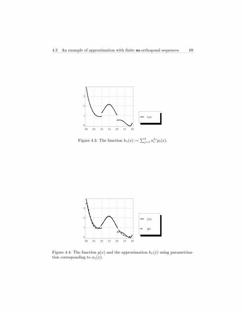
4.3 An example of approximation with finite m-orthogonal sequences 69
0.0 0.5 1.0 1.5 2.0 2.5 3.00
1
2
3
h1HxL
Figure 4.3: The function h1(x) :=∑3j=1 α
φ1
i pi(x).
0.0 0.5 1.0 1.5 2.0 2.5 3.00
1
2
3
gHxL
h1HxL
Figure 4.4: The function g(x) and the approximation h1(x) using parametriza-tion corresponding to φ1(x).
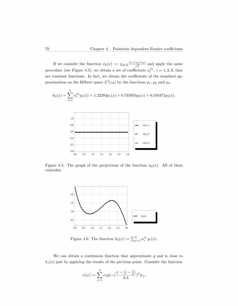
70 Chapter 4. Pointwise dependent Fourier coefficients
If we consider the function φ2(x) := χ[0,3](e1+e2+e3)√
3and apply the same
procedure (see Figure 4.5), we obtain a set of coefficients αφ2
i , i = 1, 2, 3, that
are constant functions. In fact, we obtain the coefficients of the standard ap-
proximation on the Hilbert space L2(υ0) by the functions p1, p2 and p3,
h2(x) =
3∑i=1
αφ2
i pi(x) = 1.22283p1(x) + 0.735055p2(x) + 0.104471p3(x).
0.0 0.5 1.0 1.5 2.0 2.5 3.00.0
0.2
0.4
0.6
0.8
1.0
<Φ2,e3>
<Φ2,e2>
<Φ2,e1>
Figure 4.5: The graph of the projections of the function φ2(x). All of themcoincides.
0.0 0.5 1.0 1.5 2.0 2.5 3.0
0.5
1.0
1.5
2.0
h2HxL
Figure 4.6: The function h2(x) :=∑3j=1 α
φ1
i pi(x).
We can obtain a continuous function that approximate g and is close to
h1(x) just by applying the results of the previous point. Consider the function
ψ(x) :=
3∑j=1
exp(−(x− (j − 1
2 )
0.4)2)ej ,

4.3 An example of approximation with finite m-orthogonal sequences 71
and define the function (see Figure 4.7)
φ3(x) :=ψ(x)
‖ψ(x)‖, x ∈ [0, 3].
In this case, the pointwise dependent Fourier coefficients that give the ap-
proximation h3(x) =∑3i=1 α
φ3
i (x)pi(x) are
αφ3
i (x) =
∑3j=1(
∫[j−1,j]
pigdυ0)exp(−(x−(j− 1
2 )
0.4 )2)∑3j=1(
∫[j−1,j]
p2i dυ0)exp(−(
x−(j− 12 )
0.4 )2), i = 1, 2, 3.
0.0 0.5 1.0 1.5 2.0 2.5 3.00.0
0.2
0.4
0.6
0.8
1.0
<Φ3,e3>
<Φ3,e2>
<Φ3,e1>
Figure 4.7: The graph of the projections of function φ3(x).
Figure 4.8 shows g(x) and the approximation h3(x) that is continuous by
the construction.
0.0 0.5 1.0 1.5 2.0 2.5 3.00
1
2
3
gHxL
h3HxL
Figure 4.8: The function g(x) and the approximations h3(x) using parametriza-tion corresponding to φ3(x).
The results on the continuity of the pointwise dependent Fourier coefficients
can be applied to obtain the corresponding errors of this kind of approximation.

72 Chapter 4. Pointwise dependent Fourier coefficients
If φ, φ′ ∈ L1(υ,X ′) satisfy that there is an ε > 0 such that both φ and φ′ are
ε-lower bounded with respect to the corresponding n-orthogonal sequence (as in
the case of the example), we can obtain bounds for the distances ‖αφi −αφ′
i ‖L2(υ),
in terms of ‖φ−φ′‖L1(υ,X′) following the technique given in the proof of Theorem
4.2.3. Therefore, we can also obtain a bound for the L1(υ)-norm of the difference
between the approximations associated to the corresponding functions φ and φ′,
the 1-errors E1(g, φ) and E1(g, φ′) and a bound for the difference between them
using the procedure given in the proof of Corollary 4.2.5.
Remark 4.3.6. As a concluding remark, we want to point out that Figure 4.8
tries to show that our approach is fundamentally different from the classical one.
This procedure —that weights every function fi with a Fourier coefficient that
depends on the parametrized measure and it is in fact a function itself depend-
ing also on the variable— produces a non-linear approximation of the original
function g. That is, consider that our function g is the result of sampling a
signal during an interval of time with length ∆T (in the precedent example, the
interval is [0, 3], i. e., ∆T = 3. Then we choose functions fi (in the example
p1(x), p2(x), p3(x)) according with the shape of g and we can produce the two
approximations showed in the example. Suppose that these three functions are
so suitable in shape that the Hilbert space approximation is very good. Now
we sample again the signal and we obtain a new function g. If we are interested
in keeping the same functions fi, it is not guaranteed that the shape of them is
suitable for this new approximation of g. In fact, Hilbert’s approximation can
be very bad. In our approach, parametrized Fourier coefficients avoid this and
allow to keep the same bases of functions during iterative approximations. Con-
sequently, our procedure is a natural framework for a dynamic approximation
of functions depending on one parameter for example the time. In the following
section, we show how this technique can be applied to a real problem.
4.4 Application to acoustic data
In the previous sections we have developed our approximation considering a
function g that mimics the true signals in some applied areas as it can be
Physics. In this section we are going to present an analysis of a true signal
coming from the field of Acoustics. In order to be consistent we are going to

4.4 Application to acoustic data 73
use the same sequence of functions that in the previous section. We will see
that our technique is so flexible that functions that are not adequate “a priori
”because its shape does not fit the shape of the signal, can be used in our case.
Our approximation produces better results that the corresponding standard
approximation.
We are going to use a particular example related to the Acoustics, more
precisely to the Sonic Crystals. These are periodic arrangements of scatterers
embedded in a medium with different physical properties -in our case cylinders
of a rigid material embedded in air- [44]. These structures when are considered
as an infinite periodic medium - eigenvalue problem- present ranges of frequen-
cies where the transmission of waves is forbidden. These ranges are known as
band gaps (BGs). In the last years, an increasing interest has appeared in the
potential exploitation of SC as environmental noise barriers [56], [57]. However,
the acoustical properties of SC depend on several factors showing some partic-
ularities in their attenuation properties. For example, the size and position of
the BGs depend on several factors such as the direction of incidence of the wave
on the SC and the type of arrangement of the scatterers [58]. As a consequence,
the development of the screens based on SC is not a trivial process. An example
of such type of structures can be seen in Figure 4.9.
Figure 4.9: Example of Noise barrier based on a Sonic Crystal.
When a finite structure is considered the correct understanding of these
Band Gaps implies Multiple Scattering Theory [12], [65]. Then waves are

74 Chapter 4. Pointwise dependent Fourier coefficients
not transmitted throughout the structures due to the appearance of evanes-
cent modes (see [53, 54, 55]). In this section we are dealing with one of these
evanescent modes that are the modes that cannot be transmitted through the
structure. The physical nature of such modes remains elusive and recent de-
velopments has allowed to clarify part of its nature. But the comparison of
experimental measurements with theoretical models implies having good ap-
proximations of such a kind of signals. In this section we will try to show that
orthogonal functions respect to vector measures could be an interesting tool in
such kind of phenomena. If we measure the acoustic pressure between two rows
of a SC, we observe a signal corresponding to an evanescent mode (see Figure
4.10). That is, a mode which amplitude decreases as the wave flies throughout
the periodic structure.
Figure 4.10: Measurement of normal modes (b1, b2) in front of evanescent modes(a1, a2) and (c1, c2).
In order to make clear the comparison with the precedent approximations
we are going to use the same finite sequence of n0-orthogonal functions (n0 de-
fined as before; see 4.3.5), shown in Figure 4.1 and also the same parametriza-
tions φ2(x), that provide the same coefficients than the standard approximation
on the Hilbert space L2(υ0) by the functions p1, p2 and p3, and φ3(x). The
signal to be approximated is represented in Figure 4.11.
If we apply our approximation with parametrization corresponding to func-
tion φ2(x), we obtain the result shown in Figure 4.12. The result is not surprising
because “a priori ”the shape of the functions considered for our approximation
is not the adequate for the shape of the signal, keeping apart the oscillations of
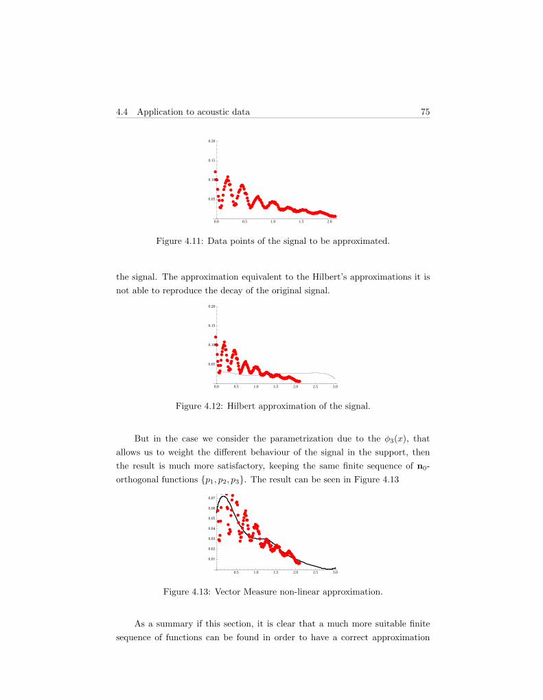
4.4 Application to acoustic data 75
0.0 0.5 1.0 1.5 2.0
0.05
0.10
0.15
0.20
Figure 4.11: Data points of the signal to be approximated.
the signal. The approximation equivalent to the Hilbert’s approximations it is
not able to reproduce the decay of the original signal.
0.0 0.5 1.0 1.5 2.0 2.5 3.0
0.05
0.10
0.15
0.20
Figure 4.12: Hilbert approximation of the signal.
But in the case we consider the parametrization due to the φ3(x), that
allows us to weight the different behaviour of the signal in the support, then
the result is much more satisfactory, keeping the same finite sequence of n0-
orthogonal functions p1, p2, p3. The result can be seen in Figure 4.13
0.5 1.0 1.5 2.0 2.5 3.0
0.01
0.02
0.03
0.04
0.05
0.06
0.07
Figure 4.13: Vector Measure non-linear approximation.
As a summary if this section, it is clear that a much more suitable finite
sequence of functions can be found in order to have a correct approximation

76 Chapter 4. Pointwise dependent Fourier coefficients
from the Hilbert space point of view but, when a determined sequence have to
be kept for doing the approximation of different signals which shape can change
in different time intervals, this procedure based on the orthogonality respect to
a vector measure is revealed as an interesting tool that provides approximations
that reproduce correctly the shape of the original signal.

References
[1] G. Alexits, Convergence problems of orthogonal series. Pergamon Press,
New York, 1961.
[2] C. D. Aliprantis and O. Burkinshaw, Positive Operators, Academic Press,
New York, 1985.
[3] C.D. Aliprantis and K.C. Border, Infinite dimensional analysis, Springer,
Berlin, 1999.
[4] N. I. Akhiezer, The classical Moment Problem, Oliver and Boyd, London,
1965.
[5] R. G. Bartle, N. Dunford and J. T. Schwartz, Weak compactness and vector
measures, Canad. J. Math. 7 (1955), 289-395 .
[6] G. Bennet, Unconditional convergence and almost everywhere convergence,
Z. Wahrsch. Verw. Gebiete 34 (1976), 135-155.
[7] C. Bessaga, A. Pelczynski, On bases and unconditional convergence of series
in Banach spaces, Studia Mathematica, 17 T.XVII.(1958), 151-164.
[8] C. Berg and G. Valent, The Nevanlinna parametrization for some indeter-
minate Stieltjes moment problems associated with birth and death processes,
Methods Appl. Anal, 1 (1994), 169-209.
[9] J. M. Calabuig, J. Rodrıguez and E. A. Sanchez Perez, On the structure of
L1 of a vector measure via its integration operator, Integral Equations and
Operator Theory 64 (2009), 21-33.
77
78 References
[10] J. M. Calabuig, F. Galaz Fontes, E. Jimenez Fernandez and E. A. Sanchez
Perez, Strong factorization of operators on spaces of vector measure inte-
grable functions and unconditional convergence of series, Mathematische
Zeitschrift 257 (2007), 381-402.
[11] L. Carleson, On convergence and growth of partial sums of Fourier series,
Acta Math. 116 (1966), 135-157.
[12] Y. Chen and Zhen Ye Theoretical analysis of acoustic stop bands in two-
dimensional periodic scattering arrays Phys. Rev. E ,64, (2001), 036616.
[13] T. S. Chilara, On indeterminate Hamburger moment problem, pacific Jour-
nal of Mathematics. Vol. 27, No.3, 1968.
[14] G. Cohen and M. Lin, Extensions of the Menchoff-Rademacher theorem
with applications to ergodic theory, Israel J. Math. 148,1 (2005), 41-86.
[15] G. P. Curbera, Banach space properties of L1 of a vector measure, Proc.
Amer. Math. Soc. 123(1995), 3797-3806.
[16] G. P. Curbera and W. J. Ricker, Banach lattices with the Fatou property
and optimal domains of kernel operators, Indag. Math. (N.S.) 17 (2006),
187-204.
[17] G. P. Curbera and W. J. Ricker, Vector measures, integration and applica-
tions, in: Positivity, in: Trends Math., Birkhauser, Basel (2007), 127-160.
[18] A. Defant, Variants of the Maurey-Rosenthal theorem for quasi Kothe func-
tion spaces, Positivity 5 (2001), 153-175.
[19] A. Defant and K. Floret, Tensor norms and operator ideals. North Holland
Math. Studies, Amsterdam, 1993.
[20] A. Defant and M. Junge, Maximal theorems of Menchoff-Rademacher type
in non-commutative Lq-spaces. J. Funct. Anal. 206 (2004), 322-355.
[21] A. Defant and M. Junge, Menchoff-Rademacher type theorems in vector-
valued Banach function spaces. Bull. Belg. Math. Soc. Simon Stevin 14,
(2007), 473-482.
[22] R. del Campo, A. Fernandez, I. Ferrando, F. Mayoral and F. Naranjo,
Multiplication Operator on spaces of integrable functions with respect to a
vector measure, J. Math. Anal. Appl. 343 (2008), 514-524.

References 79
[23] R. del Campo and E. A. Sanchez Perez, Positive representations of L1 of
a vector measure, Positivity, 11 (2007), 449-459
[24] J. Diestel, Sequences and Series in Banach Spaces, Springer-Verlag New
York, Inc. 1984.
[25] J. Diestel and J. J. Uhl, Vector Measures, Math. Surveys, vol. 15, Amer.
Math. Soc., Providence, RI, 1977.
[26] J. Dieudonne, History of Functional Analysis, North Holland, Mathematics
Studies, Amsterdam 1981.
[27] P. Enflo, Banach space with basis without a normalized monotone basis,
Ark. Math, 1973.
[28] A. Fernandez, F. Mayoral, F. Naranjo, C. Saez and E.A. Sanchez-Perez,
Spaces of p-integrable functions with respect to a vector measure, Positivity
10 (2006), 1-16.
[29] A. Fernandez, F. Mayoral, F. Naranjo, C. Saez and E. A. Sanchez Perez,
Spaces of integrable functions with respect to a vector measure and factor-
izations through Lp and Hilbert spaces Journal of Mathematical Analysis
and Applications, 330 (2007), 1249-1263
[30] I. Ferrando and E. A. Sanchez Perez, Tensor product representation of the
(pre)dual of the Lp-space of a vector measure, Journal of the Australian
Mathematical Society 87 (2009), 211-225.
[31] I. Ferrando and J. Rodrıguez, The weak topology on Lp of a vector measure,
Topology and its Applications 155 (2008), 1433-1444.
[32] J. Flores, Problemas de mayoracion en clases de operadores entre retıculos
de Banach, Ph. D. Thesis Univ. Complutense de Madrid, 2001.
[33] D. H. Fremlin, Measure Theory, vol. 2: Broad Foundations, Torres Fremlin,
Colchester, 2001.
[34] L.M. Garcıa-Raffi, D. Ginestar and E.A. Sanchez Perez, Integration with
respect to a vector measure and function approximation. Abst. Appl. Anal.
5,4 (2000), 207-226.

80 References
[35] L.M. Garcıa-Raffi, D. Ginestar and E.A. Sanchez Perez, Vector measure or-
thonormal systems and self-weighted functions approximation. Publications
of RIMS. 41,3(2005), 551-563.
[36] L.M. Garcıa-Raffi, E.A. Sanchez Perez, J.V. Sanchez Perez, Commutative
sequences of integrable functions and best approximation with respect to the
weighted vector measure distance. Integral Equations and Operator Theory.
54(2006), 495-510.
[37] E. Jimenez Fernandez, M. A. Juan and E.A. Sanchez-Perez, A Komlos The-
orem for abstract Banach lattices of measurable functions J. Math. Anal.
Appl. DOI 10.1016/j.jmaa.2011.05.010.
[38] M.I. Kadec, A. Pelczynski, Lacunary sequences and complemented sub-
spaces in the spaces Lp, Studia Mathematica, T.XXI. (1962), 161-176.
[39] M. Krein, D. Milman and M. Rutman, A note on basis in Banach spaces,
Comm. Inst. Sci. Math. Mec. Univ. Kharkoff (4) 16 (1940), 106-110.
[40] D. R. Lewis, Integration with respect to vector measures, Pacific J. Math.,
33 (1970), 157-165.
[41] D. R. Lewis, On integrability and summability in vector spaces, Illinois J.
Math. 16, (1972), 294-307.
[42] J. Lindenstrauss and L. Tzafriri, Classical Banach Spaces II, Springer,
Berlin, 1979.
[43] C. Linton, Mand Evans D.V. The interaction of waves with arrays of ver-
tical circular cylinders J. Fluid Mech. 215 (1990), 549-569.
[44] R. Martınez-Sala ,J. Sancho, J.V. Sanchez-Perez ,V. Gomez ,J . Llinares
and F. Meseguer Sound attenuation by sculpture, Nature (1995), 378-241.
[45] D. Mensov, Sur les series de fonctions orthogonales I, Fund. Math. 4 (1923),
82-105.
[46] D. Mensov, Sur les series de fonctions orthogonales II, Fund. Math. 10
(1927), 375-420.
[47] R. Nevanlinna, Asymptotische Entwicklungen beschrankter Funktionen und
das Stieltjessche Momentenproblem, Ann. Acad. Sci. Fenn. Ser. A (5) 18
(1922), 52.

References 81
[48] S. Oltra, E.A. Sanchez Perez and O. Valero, Spaces L2(λ) of a positive vec-
tor measure λ and generalized Fourier coefficients, Rocky Mountain Math.
J. 35,1(2005), 211-224.
[49] S. Okada, W.J. Ricker and E.A. Sanchez Perez, Optimal domain and in-
tegral extension of operators acting in function spaces. Operator Theory:
Advances and Applications, 180. Birkhauser Verlag, Basel, 2008.
[50] P. Ørno, A note on unconditionally converging series in Lp, Proc. Amer.
Math. Soc. 59,2 (1976), 252-254.
[51] H. Rademacher, Einige Satze uber Reihen von allgemeinen Orthogonalfunk-
tionen, Math. Ann. 87(1922), 112-138.
[52] M. Riesz, Sur le probleme des moments et le theoreme de Parseval corre-
spondant, Acta Sci. Math. (Szeged) 1 (1923), 209-225.
[53] V. Romero-Garcıa, J.V. Sanchez-Perez, S. Castineira Ibanez, and L.M.
Garcia-Raffi. Evidences of evanescent bloch waves in phononic crystals,
Appl. Phys. Lett. 96, (2010), 124102.
[54] V. Romero-Garcıa, J.V. Sanchez-Perez, and L.M. Garcia-Raffi. Modes in
sonic crystals: Complex dispersion relation and supercell approximation, J.
Appl. Phys. 108, (2010), 044907.
[55] V. Romero-Garcıa, J.V. Sanchez-Perez, and L.M. Garcia-Raffi. Propagating
and evanescent properties of double-point defects in sonic crystals, New.
Jour. Phys. 12, (2010), 083024.
[56] J.V. Sanchez-Perez, C. Rubio,R. Martınez-Sala,R. Sanchez-Grandia and V.
Gomez, Acoustic barriers based on periodic arrays of scatterers Appl. Phys.
Lett. 81 (2002) 5240.
[57] J. Sanchez-Dehesa,V. M. Garcia-Chocano,D. Torrent,F. Cerveraand S.
Cabrera, Noise control by sonic crystal barriers made of recycled materials
arXiv:1004.2570v1 [cond-mat.mtrl-sci] 2010.
[58] J.V. Sanchez-Perez,D. Caballero,R. Martınez-Sala,C. Rubio,J. Sanchez-
Dehesa,F. Meseguer,J. Llinares and F. Galvez,Sound Attenuation by a Two-
Dimensional Array of Rigid Cylinders, Phys. Rev. Lett. (1998) 80, 5325.
[59] E.A. Sanchez Perez, Vector measure orthonormal functions and best ap-
proximation for the 4-norm. Arch. Math. 80(2003), 177-190.

82 References
[60] E. A. Sanchez Perez, Compactness arguments for spaces of p-integrable
functions to a vector measure and factorization of operators through
Lebesgue-Bochner spaces. Illinois J. Math. 45 3 (2001), 907-923.
[61] E. A. Sanchez Perez, Vector measure duality and tensor product repre-
sentation of Lp spaces of vector measures Proceedings of the American
Mathematical Society, 132 (2004), 3319-3326.
[62] J. Stieltjes Recherches sur les fractions continues. Annales de la faculte des
sciences de Toulousse, 1a serie, tome 8, no 4, p J1-J122, 1894.
[63] G. Szego, Orthogonal Polynomials, 4th ed. Providence, RI: Amer. Math.
Soc., p. 33, 1975.
[64] P. Wojtaszczyk, Banach spaces for analysts, Cambridge University Press,
Cambridge, 1991.
[65] F. Zaviska The deflection of electromagnetic waves on parallel, infinite long
orbital cylinder Ann. Phys. 40 (1913), 1023-1056.