vector calculus - wordpress.com · 433 3^1 (?ottiellumnerattgcibrarg jllrara,jfanhork...
TRANSCRIPT
433
3^1
(?ottiell Umnerattg Cibrarg
Jllrara, Jfan Hork
BOUGHT WITH THE INCOME OF THE
SAGE ENDOWMENT FUNDTHE GIFT OF
HENRY W. SAGE1891
MATHEMATICS
DATE DUE
FFR8-

The original of this book is in
the Cornell University Library.
There are no known copyright restrictions in
the United States on the use of the text.
http://www.archive.org/details/cu31924001505803
VECTOR CALCULUS

*3Cttit)ersif£ gitu&ies g>etries
VECTOR CALCULUS
BY
DURGAPRASANNA BHATTACHARYYA, M.A.
Professor of Mathematics, Barielly College, U.P.
[Griffith Prize Thesis, 1918]
PUBLISHED BY THE
UNIVERSITY OP CALCUTTA19-20
/\Sl6-3>-3 4~
PRINTED BY ATULCHANDRA BHATTACHABYYA
AT THE CALCUTTA UNIVERSITY PBESS, SENATE HOUSE, CALCUTTA.
CONTENTS
Page
Introduction ... ... ... ... 1
Past I
I. Continuity : Differentiation of a Vector Function
of a Scalar Variable ... ... 7
II. Integrals ... ... ... ... 13
III. The Gradient ol\ a Scalar Function ... ....17
IV. The Linear Vector Function ... ..•? 24
V. The Differential Calculus of Vector Functions ... 30
VI. Integration Theorems ... ... ... 50
Part IIi
The Steady Motion of a Solid ur.der no Forces in
Liquid extending to Infinity ..-. ... 58

VECTOR CALCULUS
INTRODUCTION
In course of an attempt to apply direct vector methods to
certain problems of Electricity and Hydrodynamics, it was
felt that, at least as a matter of consistency, the foundations
of Vector Analysis ought to be placed on a basis independent
of any reference to cartesian coordinates and the main theorems
of that Analysis established directly from first principles.
The result of my work in this connection is embodied in the
present paper and an attempt is made here to develop the
Differential and Integral Calculus of Vectors from a point of
view which is believed to be new.
In order to realise the special features of my presentation
of the subject, it will be convenient to recall briefly the usual
method of treatment. In any vector problem we are given
certain relations among a number of vectors and we have
to deduce some other relations which these same vectors
satisfy. Now what we do in the usual method is to resolve
each vector into three arbitrary components and thus rob it
first entirely of its vectorial character. The various characteris-
tic vector operators like the gradient and curl are also subjected
to the same process of dissection. We then work the whole
problem out with our familiar scalar calculus, and when the
necessary analysis has been completed, we collect our components
and read the result in vector language. It is of course quite
useful so far as it goes, the final vector expression of the result
o-iving not only a succinct look to our formulae but also a
2 VECTOR CALCULUS
suggestiveness of interpretation which they had been lacking
in their bulky cartesian forms. But surely, strictly speaking,
we should not call it Vector Analysis at all, but only Cartesian
Analysis in vector language. In Vector Analysis proper we
have, or ought to have, the vector physical magnitudes which
our vectors represent, direct before our minds, and this charac-
teristic advantage of being in direct close touch with the only
relevant elements of our problem is sacrificed straight away,
if we throw over our vectors at the very outset and work with
cartesian components. We sacrifice in fact the very soul of
Vector Analysis and what remains amounts practically to a
system of abridged notation for certain complicated formulae
and operators of cartesian calculus which happen to recur every
now and then in physical applications.
The one great fact in favour of this plan is that it affords
us greater facility for working purposes, this facility no doubt
arising solely from our previous exclusive familiarity with Carte-
sian Analysis. But however useful it might be in this direction,
and generally in making the existing body of Cartesian Analysis
available for vector purposes, the process, I venture to think,
is at best transitional, and the importance of the subject and
the importance of our thinking of vector physical magnitudes
direct as vectors, alike seem to demand that the whole of this
branch of Analysis should be placed on an independent basis.
But there is a peculiar difficulty at the very outset. Histori-
cally, most of the characteristic concepts of Vector Analysis,
like the divergence and curl, had been arrived at by the physicist
and the mathematician in course of their work with the Cartesian
calculus and had even become quite familiar before the
possibility of Vector Analysis as a distinct branch of mathematics
by itself was explicitly recognised. The vector analyst at
first then starts from these old concepts which happen also
to be the most fundamental, but it is his object right from the
beginning to exhibit them no longer in their cartesian forms,
but in terms of the characteristic physical or geometrical
attributes which they stand for. Very often now a question
INTRODUCTION 3
of selection arises from among the number of ways in which
the same concept may be denned, different definitions being
framed according to the different points of view from which
the subject is intended to be developed. The physicist—who,
by the way, makes the greatest practical use of Vector Analysis
and whose sole interest also in the subject is determined by
the service it renders him in his work—aims, first of all, at
his definition representing most directly a familiar physical
fact or idea; but, at the same time, and very naturally too, he
holds the possibility of the definition yielding quite easily
his useful working formulae, of equally vital importance. But,
unfortunately enough, these two distinct aims of the physicist
are irreconcileable with each other, the most natural definition
from the physical point of view leads to the useful transfor-
mation formulas of Physics only with the greatest difficulty,
and the definition that yields these formulae with any facility
is generally hopelessly artificial from the physical point of
view.* It is this irreconcilability of the two distinct purposes
of the physicist which, I venture to suppose, is directly respon-
sible for the persistence of cartesian calculus in Vector Analysis.
For what is done is that definitions are first framed with a
view to direct summing up of the simplest appropriate
physical ideas, but then the necessity almost inevitably arises of
seeking cartesian expressions for working purposes, for making
Vector Analysis a serviceable and at the same time an easily
manageable tool in the hands of the physicist.
I may just illustrate my point by recalling how the usual
definitions of the two most characteristic concepts of Vector
* Reference may be made here to a paper by Mr. E. B. Wilson in the
Bulletin of the American Math, floe, vol. 16, on Unification of Vectorial
Notations, where he criticises the artificiality in the definitions of divergence
and curl by an Italian mathematician, Burali Forti, which were chosen
solely with a view to their adaptability for establishing the working formulae
of Vector Analysis with ease. Thus Burali Forti's definition of divergence is
div V=a. [grad (a. v) + curl (axv)], where a is any oonstant unit veotor.
This has certainly no direct connection with any intrinsio property of the
divergence, physical or otherwise.
4 VECTOR CALCULUS
Analysis have been adopted from the simplest physical ideas
which immediately identify them. Thus the idea of divergence
is taken directly from Hydrodynamics, and keeping before our
minds the picture of fluid leaving (or entering) a small closed
space, we define the divergence of a vector function at a point
as the limit of the ratio, if one exists, of the surface-integral *
of the function over a small closed space surrounding the point
to the volume enclosed by the surface, a unique limit being
supposed to be reached by the closed surface shrinking up to a
point in any manner.
Again, it is found that some vector fields can be specified
completely by the gradient of a scalar function, so that the line
integral t of the vector function along any closed curve in
(simply connected) space would vanish. Thus the work done is
nil along any closed path in a conservative field of force. But
in case the vector function cannot be so specified, an expression
of this negative quality of the function at a point is naturally
sought in its now non-evanescent line integral along a small
closed (plane) path surrounding the point. The ratio of this
line integral to the area enclosed by our path generally approa-
ches a limit as the path shrinks up to a point, independently of
its original form and of the manner of its shrinking, but dep-
ending on the orientation of its plane. The limit moreover has
usually a maximum value, subject to the variation of this
orientation, and a vector of magnitude equal to this maximumvalue and drawn perpendicular to that aspect of the plane which
gives us the maximum value is called the curl of the original
vector function.
Now these definitions, embodying, as they do, the most
essential physical attributes of divergence and curl, must be
regarded as perhaps the most appropriate ones that could be
given from the physicist's point of view. But then comes the
* By the surface integral of a vector function, we always mean the surface
integral of its normal component.
+ By the line integral of a vector function, we always mean the line inte-
gral of its tangential component.
INTRODUCTION 5
practical problem of deducing from these definitions the working
rules of manipulation of these operators. The direct deduction
being extremely difficult,* the already acquired facility in
working cartesian calculus is naturally utilised for the purpose,
and thus is reached the present position of Vector Analysis
which I have already described.
The only way out of the dilemma would seem to be found
by ignoring altogether both of these two specific interests of the
physicist and looking straight, without any bias, to the require-
ments of Vector Analysis as a branch of Pure Mathematics by
itself. And paradoxical though it may sound, this course
perhaps would ultimately best serve the physicist's ends also.
At any rate, no free development of any science is certainly
possible, so long as we require it at every step to serve some
narrow specific end.
We ask ourselves then, what should be the most natural
starting point of the Differential Calculus of Vectors ? All our
old familiar ideas of differential calculus suggest at once that,
whatever the ultimately fundamental concepts might be, we
should begin by an examination of the relation between
the differential of the vector function (of the position of a point
P in space) corresponding to a small displacement of the
point P and this displacement. This very straightforward line'
of enquiry I propose to conduct here, and it will be seen how
in a very natural sense we can look upon the divergence and
curl as really the fundamental concepts of the Differential
Calculus of vectors, and how this new point of view materially
simplifies our analysis.
The first three sections are preliminary. In the first two I
summarise the definitions of continuous functions and of Inte-
grals and briefly touch upon just those properties which I
require in course of my work. The third is devoted to the
Gradient of a scalar function. The real thesis of the paper I
* Compare, for instance, the difficulty encountered by Mr. E. Cunning-
ham in a paper on the Theory of Functions of a Real Vector in the Proceedings
of the Lond, Math. Soc, vol. 12, 1913.
6 VECTOR CALCULUS
begin in the fourth section where I consider the Linear Vector
Function only with a view to developing what I have called the
scalar and vector constants of the linear function, and although
there is nothing very special about these ideas themselves, they
will be found to lead very naturally to the concepts of Diver-
gence and Curl and have been made here the foundation on
which my Differential Calculus is built. The fifth section is
devoted to that Differential Calculus and in the sixth I consider
a few Integration Theorems and the divergence and curl of an
integral with a view to showing with what ease these operations
can be performed from my point of view.
Notation.
With regard to notation I use CHbbs' here, although some
of its features are obviously meant to suggest easy ways of
passing from Cartesian formulae to vector, and vice versa, with
which of course I am not at all concerned.
For convenience of reference I reproduce the notation for
the multiplication of vectors.
If A, B are any two vectors,
the scalar product of A, B is A.B=|A
||B
|cos 6, and the
vector product is A x B which is a vector of magnitude| A
|
|B
|sin 0, and in direction perpendicular to both A and B
;
|A
| , |B
|denoting the tensors of A and B and 6 the angle
between them.
Again, if A, B, C are any three vectors, the notation
[ ABC ] is used for any one of the three equal products
A.B x C= B.C x A= C.A x B= the volume of the parallelo-
piped which has A, B, C, for conterminous edges.
The following useful formula will occur very often :
A x (B x C) = (A.C)B- (A.B)C.
I.
Continuity : Differentiation of a. Vector
Function of a. Scalar Variable.
1. The functions we deal with will be mostly continuous. The
position of a point P in space being specified as usual by the
vector v(= OP) drawn from a fixed origin O, the function f(r)
is said to be continuous at P, if corresponding to every arbitra-
rily chosen positive number 8, a positive number t\ (dependent
on 8) can be found such that \f(r+e)—f(r) i <8, e being any
vector satisfying the inequality i « I < 17. The notation 1V1
denotes the absolute value of the scalar if V is a scalar, and the
tensor of V if V is a vector.
If we construct the vector diagram as well, that is, if by
taking another fixed point O' we draw the vector O'P' repre-
senting the value of the vector function corresponding to every
point P in the region in which the function is defined, then Qbeing a point in the neighbourhood of P and Q' the correspond-
ing point in the vector diagram, our definition of continuity
implies that any positive number 8 being first assigned, a
positive number rj can be found such that so long as the tensor
of the vector PQ is less than 17, the tensor of P'Q' will be less
than 8. It implies in other words that a sphere (of radius 17)
can be described with centre P such that points Q,' in the vector
diagram corresponding to all points CI within (not on) this
sphere will lie within a sphere of any arbitrarily small radius
8 described with centre P'.
We prove now that in the same case the angle P'O'Q',
that is, the change in direction suffered by the vector func-
tion can also be made arbitrarily small. For, in the triangle
O'P'Q',
8 VECTOR CALCULUS
A Asin P'O'Q' _ sin P'Q'O' ^ 1
P'Q' O'F *0'P'
Hence, sin P'O'Q' *g|J.
But P'Q' can be made arbitrarily small, and O'P' is
supposed to be finite. Henee sin P'O'Q' and therefore also the
angle P'O'Q' can be made arbitrarily small. It follows that our
continuous vector functions are continuous in direction as well.
2. The function / (r) is said to have a limit at P, if Qbeing any point in the neighbourhood of P we have the same
limiting value of the function no matter in what manner Qapproaches P continuously.
If the function is continuous at P, the limit exists at P and
is equal to the value of the function at P, and conversely.
If the limit does not exist at P, then either of two things
may happen : (i) there may be different limiting values for
different approaches to P ; or (it) there may be no definite
limiting value for any approach or some approaches. In either
case the function is discontinuous at P.
A third kind of discontinuity arises when the limit exists
at P, but this limit is not equal to the value of the function at P.
But, as has been remarked already, we shall concern our-
selves practically with continuous functions alone, and an
examination of the sort of peculiarities we have just noticed, of
what has been described as the Pathology of Functions would
be out of place here. The only discontinuity we shall come
across is the infinite discontinuity which arises when| f (v)
|
tends to infinity at P.
3. Turning our attention then to continuous functions
alone, we note that the sum and the scalar and vector products
of two continuous vector functions are continuous also. The
case of sum is almost self evident, and we prove now that if V 1}
V2
are two continuous vector functions, the scalar product
Vl-V g is continuous.
CONTINUITY.- DIFFERENTIATION 9
Let V',, V'B denote the values of the functions at a point
r+e in the neighbourhood of the point r. We have only to showthat for any positive number 8 assigned in advance, a positive
number -q can be found such that
|V'1-V'
a-V 1-V
2 |<8,
for all vectors t satisfying|e
|
<ij.
Now v\-Y' % -v l-v t =iv l + <y\-v l )y\y,
+ (V'1-V I)]-V, •V.sV, -(V/-VJ
+V a -(V 1'-V 1 ) + (V1'-V 1 )-(V 2'-V a ),
which is not greater than|V 1 |
|V a'-V a | + |
V a | |Y l '-V 1 |
+ |V/-V,
I I
V a '—
V
2 I, since the magnitude of the scalar
product of two vectors is not greater than the product of their
tensors.
Hence, since the absolute magnitude of the sum of any
number of quantities is not greater than the sum of their abso-
lute magnitudes, we have
|V 1 '>V a'-V
I-V a I* I
V,I|V,'-V.
I
+i
v,i l
y 1'-y
l i+
i
V/-V,i i
v s'-v a i
But since V\, V2are continuous,
|Vj'—V 1 |
<any arbitrary 8X ,
provided only|e
|< the
corresponding 1?!, and | V 8 '—
V
a | < 8 2 ,-q
2
Of the two numbers i?!-17 a , let rj^rj^
;
then provided|e
| <,„ |V 1'~V 1 |
<8Xand
|V 2'-V 2 |
<8 a ,
and therefore |V^-V.'-V^V,
|< |
V x | 8, + [V.
f8,+S.S,.
Again, since|"V x | , |
V B ]are supposed to be finite, given any
positive number 8, we can always find S1and 8 2 such that 8>
|Vi |Sa + |V, 18,+M,-
Choosing such values now of 8, and 8 2 , we have
IV'1
-V',-'V 1-V 1 I
<8, whenever|*
| <,u
which proves our theorem.
Similarly we prove that V, x V2
is also continuous. A{
10 VECTOR CALCULUS
4. If we consider in particular the continuous vector func-
tion of a scalar variable, we can easily adapt the argument of
the usual scalar calculus and prove the theorems associated with
continuity in that calculus. If r=f (t) be the function consi-
dered, t being the scalar variable, we can prove in particular
that if r x=f (ti) and *»
2 =/ (t2 ) and p is any number
such that |*,i|<p<|**2|> ^en there is a value of t lying
between tland t 2
for which \f(t) | =p. In other words, as t
varies continuously from t1to t 2 ,
the tensor of v assumes at least
once every value lying between ttand t 2 .
It can further be proved that if F (r) is any continuous func-
tion, scalar or vector, of v where v itself is a continuous function
of a scalar variable t, then F is a continuous function of t.* In
case F is a scalar function, it follows that if F,, F2 are
the values of F respectively for t= lt
and t= t2 , then as t
varies continuously from t1
to t 2) F assumes at least once
every value lying between Fj and F 2 ; and when F is a vector
function, it is the tensor of F that assumes, as t varies conti-
nuously from il
to t 2 , at least once every value lying between
the tensors of F corresponding to t=ttand t=t
2.
5. If for the continuous vector function v=f(f), a unique
limit exists of **;—sLi-2 as t' approaches t from either side,
(i.e. from values less than t to t and from values greater than
t to t), then this limit is called the differential coefficient of
* Proof. We have to show that if 5 is assigned in advance, i) can be
found such that
lF(/)-F(r)l ZS,
when 1 t!—t \ Lv, r' being the valne of r corresponding to t=t'.
Now since F(r) is a continnous function of ), an tj, can be found such that
1 F(r')-F(f) 1 ZS, when 1 r'-rl LVi-
Again, since r is a continuous function of t, corresponding to this ?i„ apositive number i) can be found suoh that \ r'-rl l Vl , when \t'-t 1 Lit.
This it then is such that when \t'— t\ Lit,
1 r'-r 1 l Vl and 1 F(r')-F(r) 1 /,,
CONTINUITY: DIFFERENTIATION 11
r with respect to t and is denoted by —-=- . The function r inwt
the same ease is said to be differentiate at t.
A function r =f(t) which is continuous and differentiable
at all points in a certain region can in general be represented
by a curve in that region. The terminus of r will trace out
the curve as t goes on varying continuously, and the vector
-j— will be at each point in the direction of the tangent toCvt
the curve at that point.
If F(r) is a continuous vector function of r, it follows now
from the last article, that the vector diagram of F(»*) corres-
ponding to points lying on any arbitrary but continuous curve
r=f(t) between any two specified points P and Q, is also a
continuous curve lying between the corresponding points P'
and Q! in the vector diagram.
6. Mean value theorem for v=f{t).—If r is a continuous
and differentiable function of t for all values of t between any
two specified numbers tt
and t2 , then V
tand r 2 being the
values of r respectively for i-=txand (= t
2 , we have
rt-r, =-lf f{t i
+et i-=t l ),
where 6 is some positive proper fraction.
This is proved, precisely as in the case of the corresponding
theorem in scalar calculus, by considering the function
which is continuous for all values of t between tl
and t 2 and
vanishes for t=ttand i= t
2 , and of which therefore the differ-
ential co-efficient will vanish at some point between tl
and t2 ,
say at tt+0(t 2
— tt ),
where 6 is a positive proper fraction. This
proves our theorem.
12 VECTOR CALCULUS
Graphically, if R denotes the vector to any point on the
chord of the curve r=f(t) joining the points ttand t 2 , the
equation of the chord is
for obviously it represents for varying values t a straight line
parallel to «*3—v
xand gives R= »*
1at t= t
land R=r 2 at t=
t 2 . Our *(£)=**— R= R', say, represents then for any value
of / the difference of the vectors to points on the curve and
the chord corresponding to that value of t. If these vector
differences are now drawn from the origin for all values of t
from txto l 2) their terminii will give us another curve re-
presented by R'=*(i!), which clearly is a continuous curve
returning unto itself at the origin for t = txand i= t 2 > and the
vanishing of for some intermediate value of t implies thatdt
in course of the journey of the terminus of R' from the origin
and back to it again, there will be a position which will make
the tensor of R' or v—R stationary.
II.
Integrals.
7. The Vector Volume Integral.—Given any finite con-
tinuous volume t, if for any convergent system of sub-
divisions * of the region, the vector sum s> F„t„, where
t„ denotes any sub-region at any stage of the sub-division
and F„ the value of F at any point within the sub-region
T „, tends to a definite, unique limit as the sub-division
advances, independent of the particular convergent system of
sub-divisions used and of the particular values of F chosen
within the sub-regions t„, then this limit is called the volume
integral of the vector function F through the volume t, and
T
is written JF^t.
Without going into the question of the necessary minimum
condition for the integrability of F, we may prove without
much trouble the only theorem we require in this connec-
tion, viz., that if F is continuous at all points within a
finite region, it is integrable also through that region ;
—
the continuity of F ensuring that if F„, F„' are the values
of F at any two points in the sub-region t„, the tensor of
the difference of F„ and F„' becomes arbitrarily small as
the sub-division advances and each sub-region diminishes in
volume.
A graphical representation of the vector volume integral
may also be suggested here. Starting from any arbitrary
point O', we lay down the vectors F„t„ as in the ordinary
polygon of vectors. In the limit the polygon becomes a
continuous curve, ending say in A.' Then the arc O'A' will
represent / |F |
dr and the chord O'A7
will represent our
volume integral fFch. Since F is supposed to be integrable,
* Compare Hobson's Theory of Functions of a Real Variable, § 2S1.
14 VECTOR CALCULUS
the chord O'A' will be unique, but we may have an infinite
number of curves like O'A' according to the different orders in
which we may place the vectors F„t„ in forming the
polygon. All these curves however will have the same
length J |F
jdr and the same terminal point A'. Further, to
any point P' on any one of these curves there will corres-
pond a unique point P in the volume t, and conversely,
so that there is a one-to-one correspondence between the points in
the volume and the points on any particular curve.* Wehave also d)>' = ~Ffh, if v' is the vector O'P', so that the
tangent at any point P' on the curve is in the direction
of F at the corresponding point in the volume. It may
happen that J |F
|dr is infinite, but [FdT at the same time
exists as a finite vector. Thus the curve may make an
infinite number of convolutions, but such that the terminal
point A' is at a finite distance from O'.
8. The surface integrals.—Given any continuous surface
S in a .region where the vector function F is defined, we
form the scalar product F,» at each point of the surface,
n denoting the unit vector along the outward normal at
any point to the surface, and the surface integral, in the
usual sense, of the scalar function F.» over the surface we
call the surface integral of vector function F over the
surface and denote it by JF.w^S. In other words, for any
convergent system of sub-divisions of the surface S, if S r
is a sub-area at any stage of the sub-division and F r .n r
the value of F.n at any point within the sub-area, the unique
limit to which sF r .?/ r S r is assumed to tend as the sub-
division advances is called the surface integral of F over
the surface S. But with the advance of the sub-division
the areas S r approximate to small plane areas on the
tangent planes at points P, and the vectors w,S, ultimately
* There is of course no a priori absurdity in the idea of a one-to-
one correspondence being established between the points in a given
volume and the points on a line, for we know from the theory of
sets of points that the two aggregates have the same "power."
INTEGRALS 15
may be regarded as representing these plane areas both in
magnitude and direction. We may replace therefore the
notation jF.wrfS \bj jF.rfo-, d<r=ndS representing the ulti-
mately plane element dS both in direction and magnitude.
Forming again the vector product of F and the vector
» rS r at each point and summing up for all points and
passing to the limit in the same way, we have another
surface integral JF x ndS or JF x da-. This has been called
the skew or vector surface integral, fF.do- being the direct
or scalar surface integral. We shall always mean fF.da-
when we speak only of the surface integral of F, referring
to JF x da as the skew surface integral.
If the surface S is supposed to be continuous and to possess
moreover a continuous tangent plane at every point, the vector
n would be a continuous function over the surface, and if F
is supposed to be continuous also, both F. n and F x n will be
continuous functions and the scalar and vector surface integrals
of F over S will both exist. We shall always make this
supposition here.
9. The line integrals.—Given any continuous curve, if in
any convergent system of subdivisions, p n is the vector chord
joining two consecutive points of division at any stage of sub-
division in the system, and F„ is the value of F at any point
P of the curve between these two points of division, then the
unique limit to which 2>F n .jo n is assumed to tend as the sub-
division advances is called the line integral of F along the
curve AB. The chord p n is obviously equal to the difference
in the values of r at the two points which it connects, and our
Siintegral may be denoted by 1 F.dr. It is further clear that
with the advance of the subdivision, p„ approaches in direction
to the tangent to the curve at P, and if therefore we denote
the unit vector along the tangent at any point of the curve by
t, the integral is the samp as the line integral, in the usual
16 VECTOR CALCULUS
sense, of the scalar function F.t, and might be denoted by / F.t ds,
ds being the scalar element of arc.
We might in the same way define the vector line integral
/ Fxdr, but this will rarely occur in the present paper.
In any case we shall always suppose that the curve along
which we integrate is not only continuous, but also possesses
a continuous tangent, so that t is a continuous vector function
of the position of a point on the curve.
The following properties of the line integral follow imme-
diately from the definition.
(0
(«)
CB CA\ F.dr = - 1 F. dr
JA JBfB CP CB\ F.dr= 1 F. dr+ I F.dr, P being any point on the
JA JA JPcurve AB.
(m) If 1 is the length of the arc AB and L, U the lower
and upper limits respectively of F.t for the curve AB (which
limits are supposed to exist, though not necessarily to be
attained), then
Ll<\ F.dr £U1.isJ/-
(iv) Further, if M is some number satisfying L^M<U,
fB
we have I F.dr=Ml ; and in case F is continuous, so that F.t
JA
is continuous also, the value M is attained by F.t at some point
fB '•
P of the curve, and we have I F.dr = (F.t)=l.
Ill
The Gradient of a Scalar Function.
10. Let F(r) be a continuous scalar function of the position
of a point P (OP= r) in a given region. If Q is a point in the
neighbourhood of P, such that PQ= ah where a is a unit vector in
direction PQ and h a small positive number, then the value of
F at Q is F (r f ah). If now the limith^ ^- [F (r + ah) -
F(r)] exists as a definite scalar function (different from zero)
of a and r, this limit would measure the rate of change in the
value of the function for a displacement of P in the direction
a. Supposing the limit to exist and denoting it by f (a, r),
we have F(r+ ah)— F(r)= hf(a,r) + hiy, where y and h have
the simultaneous limit zero.
Now since h appears in the left hand side of this equation
only in the combination ah, and the first term on the right hand
side is linear in h, it follows that this term is linear in a also.
The function f (a, r) then is a scalar function linear in a ; it
vanishes moreover with a, and therefore it must be of the form
a. G (r), where G (r) is a vector function of r, independent
of a.
If the limit in question exists now for every direction a
emerging from P, the rate of change of F(r) in any direction
a is a.G(r), the maximum value of which obviously, for varying
directions a, is obtained when a is taken in the direction of Gand the magnitude of the maximum value is equal to the tensor
of G. The vector G is called the gradient of the scalar function
F. The gradient of a scalar function then may be generally
defined as a vector in the direction of the most rapid rate of
increase of the function and equal in magnitude to this most
rapid rate.
3
18 VECTOR CALCULUS
11. The same question may be looked at geometrically also.
We begin by proving* that if F (r) is a scalar function continu-
ous in a certain region and does not possess any maxima or
minima in the region, and if F is the value of the function at
any point P of the region, then there passes through P a surface
on every point of which F has the value F
For, since P is neither a point of maximum nor minimum,
all the values of F in the neighbourhood of P cannot be greater
than F , nor can all the values be less than F , and there would
be points in the neighbourhood for which F is greater than F
and there would be points also for which F is less than F .
In the neighbourhood of P then, let Q be a point such that
F >F , and R a point such that F <F . Now on accountQ P K F
of the continuity of the function, a region can be constructed
about Q. within which the fluctuation of the function is as small
as we please. Hence there exist other points near Q for which
also the value of the function is greater than F . Similarly
there exist points near R for which the function is less than F
Hence the region consists of two distinct regions in every point
of one
F<Fp .
Again, since in passing from any Q to any R along a conti-
nuous curve, F must on account of its continuity assume all the
intermediate values, it assumes the value F somewhere between
* This proof ia adapted from the solution an example in Eouth's statics,
Vol. II (Ex. 2, $ 124), where from the fact that gravitational potential is
neither a maximum nor a minimum in free space is deduced that an isolated
line cannot from part of a level surface.
of one of which F>F , and in every point of the other
THE GRADIENT OF A SCALAR FUNCTION 19
Q and R on that curve. Hence there is a continuous surface
of separation of the two regions at every point of which F=F ,
which proves our theorem.
If now the surface possesses a tangent plane at P, we take
a point P' on the normal to the surface at P in its neighbourhood.
Through this point P' also will pass a surface on every point
on which F=F,/ and PP' will be normal to both the surfaces
FP'- FPF=F and F=F . Supposing now that the limit —exists as P' moves continuously along the normal and approaches
P, a vector in the direction of this normal and equal in magni-
tude to the value of this limit is called the gradient of F(r) at P.
[P' might be on the normal on either side of the surface, and
it is assumed that the limit in question exists in either case and
that these two limits aL'e equal.]
To see that the gradient so defined gives us the most rapid
rate of increase of the function both in magnitide and direction,
we take a point Q. in the neighbourhood of P on the surface
on which P' lies. Let ZP'PQ= #. Then the rate of increase
of the function in direction PQ.
_ L ^%^-'= L €^l. |gl= (gradF)cose_QP=0 pQ PP'=0 pp e(*
of which the maximum value obviously is obtained when 0=0.
This establishes the identity of the definitions of gradient in
the present article and the last.
We denote the gradient by VF. If 8F is the change in the
value of F on account of the shift oV in the position of P, we have
8F= VF. Sr+17|Sr
|
where -q and |Br
|have the similtaneous limit zero.
12. If the shift Br is supposed to take place along a definite
continuous curve r=\(i), then as we have seen (§4, p. 10) F
would be a continuous function of t along that curve, and our
relation of the last article can be written - =yF. *-.
20 VECTOR CALCULUS
Further, if £,, t a specify any two points K, L on the curve
r—x{t) and if F„ F a are the values of F at K and L respec-
tively, we have by the Mean "Value Theorem of §6, p.ll.
'M
t- ) dennotes the value of ^- at some point M on theat /
jyjat
curve lying between K and L. That is to say,
F,-F1=(*.-0 (VP)».(J)
In particular, if the curve is a straight line in the direction of
the (unit) vector a-and /* is the length of KL, so that KL=a/i,
we may write P(r+n/()-F(?)=k(vF)„=k VF (r+adA).
where 6 is a positive proper fraction; or again, F (r+a)— Y(r)
=a.VF(r+ «a).
13. We establish now the corresponding integral formula,
for which we prove first that if/0 -
) is any vector function (not
necessarily continuous) integrable along a given curve AB, then
P
P being any variable point on that curve, the integral 1 f(r). dr
Ais a continuous function of the position of P on the curve.
P
Denote \f(r).drbyF(r), Then if Q is any other point
A
Q
r+t on the curve, we have \f(r)Jr=F(r+e), and therefore
THE GRADIENT OF A SCALAR FUNCTION 21
Q
F(r+f)-P(r)= If.dr.
P
Q
\fdr\ <\Jl, where U is the upper limitBut (see p.16)
offt for the curve AB and I is the length of the arc PQ.
Hence|F(r+e)-F(r)
|<U7,
and therefore | F(r+ t)— F(r)| can be made less than any
arbitrary positive number 8, if only I is so chosen that 8>U/j
or l<^ , which is always possible because U is supposed to be
finite. Again, since the curve is supposed to possess a continuous
tangent at P (p-lo), there is a finite portion of the curve about Pfor which the arc measured from P and the corresponding chord
increase together. It is possible therefore to take a point P'
gon the curve in such away that the arc PP' <— and also such
that the arcs corresponding to chords PQ which are less than
g|P P'
| , are less than the arc PP' and less therefore than •=?.
It follows that for all vectors e satisfying je
| < |pp'
| ,
where the arc PP'< ^j, we have|F(r+ e)— F(r)
|<8, which
proves our theorem.
14. We conclude that if f(r) is integrable along any curve
in a , continuous region, and if A is a fixed point and P any
variable point in the region, then integrating along the various
curves through A and P, we have any number of functions
p
/ f- dr, each of which is continuous for a displacement of P on
22 VECTOR CALCULUS
the curve along which the integral is calculated in any case.
Under certain conditions however (See §42), of which the
continuity off is one, the intergral is known to be independent
p
of the path of integration, and in this ease therefore J f.drA
will define a unique continuous function F(r) of the position of
P in space. Assuming these conditions to hold, and assuming
in particular thatf(r) is a continuous vector function, we shall
prove here that/= VF,
For, if f is continuous, and since in accordance with the
understanding in § 9, the unit vector t to any curve through
A and P is supposed to be continuous,/' -if is also a continuous
function of the position of a point on this curve. Hence, if P is
the point r and we consider another point r' on the curve in the
neighbourhood of P, f and t' being the values respectively of
f and t at r', then for any arbitrary 8, a positive number -q can
be found such that
\f-t'-f-t\ <S, if \r'-r\ <,,
which shows that \f'mt'
|lies between
| f- 1\+ 8 and
|
/'t
|
— 8 ; every value, in other words, off-t in the portion of the
curve between r and ?•' lies between \f't |+ 8 and | f-t
\—8.
If « denotes the vector t'— r, the integral / f-Ar lies betweenr
l[I
**I+ 8] ancl l i \f't\ - 81> l being the length of the
arc between r and /.
ButF(r+ e)-F(r)=/ /-dr.
:. P(r+ €)-F(r) lies betwern l[ \f-t \+8] and l\_ \f-t \
-8]
But 8 and therefore also I can be taken arbitrarily small
;
and with the arbitrary shortening of I the difference between the
are I and the chord|
«|becomes arbitrarily small, and the
direction of e approximates to that of t. We can write therefore
THE GRADIENT OF A SCALAR FUNCTION 2R
F(r+ c)-F(r) =£•/(>•)+|
e|
8', where S' and |e
|have the
simultaneous limit zero.
This result, which is true for all curves through A and P and
true therefore for vectors € drawn in all directions round P
shows that/*= V F.
If therefore we have any curve in the region, and 1\, 1\ are
any two points on the curve, we have
J vF-dr=f /^=P(r1)-F(r 1 )
IV
The Linear Vector Function.
15. The most general vector expression linear in r ean
contain terms only of three possible types, r, a.rb and cxr,
a, b, c being constant unit vectors. Since r, a.rb and cxr are in
general non coplanar, it follows from the theorem of the parallelo-
piped of vectors that the most general linear vector expression
ean be written in the form
\r+fi a.rb+vcxr
where \, p, v are scalar constants. The constants p, v may
moreover be incorporated into the constant vectors a and c and
we write our general linear vector function in the form
<£ (r)=\r+a.rb+ cXr,
where b only is a unit vector.
Obviously,<f>
(r) is distributive;
that is,<t>
(a+ j8)= * (a)+ <£ (/?),
and further <j> (Jcr) =k <f>(r), where A; is any constant.
1 6. Theorem.—The surface integral of<f>
(r) over any closed
surface S bears a constant ratio to the volume T enclosed by
the surface, the constant depending only on the function but
being independent of the particular surface over which we
integrate.
To prove this we integrate separately the three terms of <t> (r)
over the surface.
s sWe know J"\r.d!cr=Af?\do-=3A.T.
S
To calculate fa.rb. da- we break up the region S into thin
cylinders with axes parallel to b. Since the surface is closed,
each of these cylinders like PQ will have an even number of
intersections with the surface, as in the usual proof of Green's
Theorem. It is enough to consider here the case where there
are two intersections only, the extension to the general case being
the linear Vector function at
obvious as in that proof. If then da' and da are the elements of
surface on S enclosed by the cylinder PQ, we have
6. da- =—b. d<r=area,of the cross section of the cylinder PQ.Let P be the point r, then if x is the length of the
cylinder, Q is the point r+xb, b being a unit vector; andthe sum of the contributions of da and da' to the surface integral
approximates, as the cross section of the cylinder diminishes, to
a.(r+xb) b. da'+ a. r b. da
i.e., to a.b xb.da'
i.e., to a.bdr, where dT is the volume of the cylinder PQ.Hence the whole surface integral
S
$a.rb.da=a'bT.
"We may just by the way note from the symmetry of the
result that fa.rb.da=fb.ra.da=a'bT, and this result holds for
any two arbitrary constant vectors a, b. That is, for any two
constant arbitrary vectors a,b we have
a.$rb.da=b.fa.r da=a'bT, which shows moreover that
/r6.do-=6T and jd.rda=aT.
Generally therefore $ra.da=fa.rda=aT, a being any
constant vector.
To return to our proof now, we have to integrate fc X r.da.
Putc=ax/?, so that c X r=a.r/3—/J.ra (p. 6)
Hence /c X r.da=fa.rp-da—J/J.raJ<r=a-/3T—a7?T=0r
We have therefore finally
r<Kr).do-=3A.T+a.&T
i.e., — /<£(». da=3\+a.t=I>, say,
which proves our theorem.
17. The skew surface integral of cf>(r) over any closed
surface S divided by the volume T enclosed by the surface
is a constant vector, this constant vector depending, on the
function <Kr)> but being independent of the surface over which we
perform the integration.
26 VECTOlt CALCULUS
Proof. We proved in the last article that fcxr.d<r=0, c
being any constant vector. It follows that /c.r x d<r=0 (p. 6),
i.e., c. JV X d<r=0, or JV X d<r=0, because c is arbitrary.
Also, fa.rb X da=b X Ja.rdcr= bx aT [§16]
Again /(c X r) X do-=$rc.dcr—fcr.d<r [p. 6]
.
=cT-3cT= -2cT [§16].
S SHence /<^>(r) X d<r=f[\r+a.rb+cx r] X do-
=-(ax6+2c)T= -CT, say;
C=— — /<£(»•) xd<r= =5-/^0" X<£(r) being a constant vector,
our theorem is established.
D and C which we find here associated with every linear
vector function, we shall always refer to as the scalar and
Vector constants respectively of the linear vector function.
18. We consider the function now
\r+ b.ra—cxr
which is immediately seen to have the same scalar constant 3X+
a.b as the original function <f>(r)=Xr+a.rb+ cXr ; and its vector
constant is— (axb+ 2c) Vhich differs only in sign from the
vector constant of <Kr)-
Further, if a, /3 are any two arbitrary vectors, we have
a.<£G3) =a.[X/3+ a -fib+ c X j8]
=j8'[Xa+6'a«-cXa]=W(a), if we call the new function
*'(r).
The two functions <j>(r)=\r+a.rb+ cxr
and <f>'(r)=\r+b'ra—cXr
may on this account be called conjugate functions.
With every linear vector function <j>(r) then is associated
another function <£'(r), characterised by the propery a.<£(/8)=/3.<£'(a) for any two arbitrary vectors a,/? and having further
the same scalar constant as <f>(r) and a vector constant differing
only in sign from that of <£(?')•
THE LINEAR VECTOR FUNCTION 27
19. Since the scalar or vector constant of the sum (or
the difference) of two linear vector functions is obviously the
sum (or difference) of the scalar or vector constants of the
two functions, it follows that the scalar constant of <t>(r) +4>'(r) is 2D and its vector constant is zero ; and that the
scalar constant of <Kr)— <£'(r) is zero an(i its vector constant
is 2C.
Obviously again the conjugate of<f>(
r) +4>'(r) 1S itself ; this
function, that is to say, is self conjugate. And the conjugate
of <f>(r)— <j>'(r)=<f>'(r)— <£(r)=— [<K»")— <£'(»•)], which is the origi-
nal function with the minus sign prefixed. Such a function
has been called skew or anti-self-conjugate.
The function <£(r)— 4>'{r) in full is
a.rb—b.ra+2cxr
= (ax&)xr+2cxr [p. 6]
= (a X &+ 2c) X r=C X r.
Hence <f>(r) can be written
=il#r) + <t>'(r)) +iW(r)- <t>'(r))
=<£,,(»') +i C xr, where 2<£„(r) has been written
for the self conjugate function <£(r)+<£'(r).
Any linear vector function <f>(r) therefore can be expressed
as the sum of two other functions one of which is self conjugate,
has the same scalar constant as <f>(r) and no vector constant,
and the other is skew, has no scalar constant and the same
vector constant as cf>(r).
The resnlt ^(f)-f(r)=Cxc shows moreover that the vector
constant of all self conjugate functions is zero.
20. The vector constant of <f>(r) may be exhibited in another
manner, for which we calculate first the gradient of the scalar
function r.<ji(r).
Since 8[r.*(r)]= (r+8r).*(r+8r)-r.*(r)
= (r+8r).[*(r)+*(8r)]-r.*(r)
=r.<j>(hr) + Sr.<t>{r) + 8r.<j>(8r)
=8r.[<£'(r)+ <Kr)]+?7 ISr
| , where ij is
28 VECTOR CALCULUS
a scalar number which has limit zero as|Sr
|tends to vanish,
it follows that V [>'•<£(?')] =<£(?) + <£'('")> an(i we caa wl'ite
*W=*V[r.*W]+iCxr.
Integrating now round any plane closed curve, we have
J<£(r).dr=AjV[r.<Kr)].cZr+!jC X r.dr.
Since >:<j>(r) is single valued, the first integral on the right hand
side is zero, because it is equal to the difference in the values
of i r.<j>(r) at the same point before and after circuiting. [p.23.]
Also J> x dr is twice the vector area enclosed by the curve,
a fact which becomes obvious by taking a new origin O' in the
plane of the curve. For if 00' =a, OP=r and OT=p, we have
r=p+ a and dr=dp, and frxdr=f(p+ a)xdp. Hence since
fdp and therefore also fa x dp vanishes, the curve being closed,
we have frxdr=foxdp which is a vector normal to the plane
of the curve and equal in magnitude to twice its area.
Thus J<t>(r).dr=±fCxr.dr=±C.frxdr=C.nS, where S
stands for the area enclosed by the curve and n a unit vector
along the normal to the plane of the curve.
The ratio ^ [<p(r).dr=C.n does not then depend on the parti-S
cular curve round which we integrate, but it depends on the
orientation of the plane of the curve, on the vector n. This
ratio obviously again attains its maximum value when n is taken
in the direction of C. The vector constant of <p(r) then is a
vector in the direction of the normal to that plane, round any
curve on which if we calculate the line integral of <j>(r) the ratio
of this integral to the area of the curve is maximum, and the
magnitude of the vector constant is equal to this maximum
ratio.
21. There is just one bit of work more in connection with
linear vector functions before we are ready for the Differential
Calculus of vector functions.
If a is any constant vector, a x <£(r) is of course also a linear
vector function of r. We proceed to find D t and C , the scalar
and vector constants of a x <£(»•).
THE LINEAR VECTOR FUNCTION 29
Integrating over any closed surface (enclosing volume T) we
have by definition
D1 T=fax<t>(r).d<T
=a.J<f>(r) X do-
=—a.C T, where C is the vector constant of <j>(r).
.•.Dl= -a.C.
Again,—
C
1T=J[aX^>(r)] xda
=J<t>(r)a.da-—jacj)(r).d(T (p.. 6),
But fa<f>(r).d<r=af<l>(r).dcr=a~DT, D being the scalar constant
of </>(r).
Also f<f>(r)a.d<r is calculated immediately by breaking up the
volume into thin cylinders with axes parallel to a, as in §16,
p. 25. Thus if OP=/ and PQ=a:a, the sum of the contributions
of the elements of area da and da' at P and Q approximates, as
the cross section of the cylinder PQ diminishes, to
(f>(r+xa) a.da-1 + <f>(r)a.da
which again, since xa,dar'=— xa.da=vol. of the cylinder
and <£(r+ xa)=(f>(r) + x<j>(a),
approximates to <j>(a)dT, T being the volume of the cylinder
PQ. Hence J>(r)a.dcr=<Ka)T
Hence finally—
C
1T=<^(a)T-aDT
VThe Differential Calculus of Vector Functions.
22. The Differential Calculus of the scalar function of a
single (scalar) variable concerns itself with the rate of change of
the function with respect to the variable. In considering in the
same way the rate of change of a vector function f (r) of the
position of a point in space, the first difficulty we meet with
is that this rate of change is different for the different directions
in which the point P may be shifted. In fact, the position of
P being specified in the usual way by the vector r drawn from a
fixed origin, a change in the position of P of magnitude h
and in the direction of the unit vector a would be denoted by
ah, and the change in the value of the function would be
f(r+ ah)—f(r). The rate of change then in the value of _/at
P for displacement of P in direction a is
L f(r+ ah)-f(r) ,
h— o h
In Gibbs' notation this is denoted by aSJf; we shall often
denote it,—perhaps a little more expressively—also by A af.
In order that the limit may exist it is necessary that_/ should
be continuous at I' in the direction a. For if f is discontinuous
in this direction, then however small h might be, \f{r \-aK)—f{r) |
would be greater than a certain positive number 8 and
therefore — J-—— I can be made greater than any arbi-
trary positive number, and therefore the limit cannot exist. But
the continuity of ./ alone in direction a cannot ensure the exis-
tence of the limit, for which it is necessary that the fluctuation
of I f(r+ ah)-f{r) as a function of h should be arbitrarily
small within a sufficiently small interval on the line a in the
neighbourhood of P. The continuity therefore is a necessary
though not the sufficient condition for the existence of the limit
in question.
CALCULTlS OF VECTOR FUNCTIONS 81
But in any case where the limit does exist as a definite
function of a and r, it is clear as in § 10, that that function
will be linear in a. We may denote therefore L ?[f(r+ ah)—
f(r)~] by 4> (a > »")» or m0I-e simply by <£ (a), where <j>(a) stands
for a linear vector function of a. The explicit presence of r in
<£(«, r) would serve to bring out the fact that the rates of
change off(r) are given by different linear vector functions at
different points P in the region.
If th'e limit exists for all directions a issuing from the point
P,—for which it is of course necessary that /"should be continuous
at P—we write for any a
dafor a. V/=<£ («),
a.ndf(r+ak)=f(r) -f A<f>(a) + kr), where y is a vector such that
|r)
|has limit zero as h tends to vanish.
Or, since h <£ («)= <£ {ah) [ §15, p. 24], if 8/ denotes the
vector increment of f corresponding to the increment 8/ of r,
*f=<K*r) + V |8r
|.
23. If the shift 8r be supposed to take place along a definite
continuous curve r=x{t), then we know (§ 4), that /would
be a continuous function of t along that curve and we would
write from our relation of the last article that
df £(8r)
dt St'
which, since <£(Sr) is a linear vector function of 8;-,
=^(1) [§15, p. 24]
Further, if tt , t
2specify any two points K and L on the curve
r= x(t), and/i and_/2 are the values of f at K and L [respec-
tively, then we have from the Mean value theorem of §6,
A -/,=('* -Offdt/M'
32 VECTOR CALCULUS
where (j^)^ denotes the value of -£ at some point M on the
curve lying between K and L. In other words
/.-'.=('.-<*) [*(£)]M ,
if, of course, a definite </> exists at every point on the curve be-
tween K and L.
In particular, if the curve is a straight line in the direction
of the (unit) vector a and h is the length of KL so that KL=a/5we may write f(r-\-ah)—J\r)—h <f>(a, r+aOk)
' =hd af{r+a6h),
assuming, of course, that d af exists at all points on the line KL.24. We shall practically always confine ourselves to func-
tions which are not only continuous within a certain region, but
are also such that d af or 4>(a) exists at every point P of
the region for all directions a round that point. If weconstruct a sphere of unit radius with P as centre, then
every point on this sphere will represent a definite direction a
issuing from P, and <£ being known for P would mean that
corresponding to every point on the unit sphere we know the
rate of change of / (at P) both in direction and magnitude.
But as to the rate of change of / at P as a whole, we cannot as
yet form any definite conception, not at least directly from our
knowledge of the function <£ at P which only brings before our
minds a bewildering diversity of the rates of change for the
infinitely many directions round P. What we naturally do there-
fore is to have an idea of some sort of average value of <jb (a)
for these directions a,—average of <£ (a) over the unit sphere
round P.
We consider then two kinds of such an average value.
Since a is a unit vector, the magnitude of the component
of <j>{a) in direction a is a.^(a). We consider first the average
of this magnitude over the unit sphere, which is
fa-<M>) dS
CALCULUS OF VECTOR FUNCTIONS 33
where dS is the scalar element of area on the surface of the
sphere at the terminus of the vector a, and S is the whole
surface S.
Since the radius of the sphere is unity, S is equal to 4ir and
is therefore equal to 3T, where T is the volume of the sphere.
Also adS=d(r the vector element of area, the normal to the
sphere at the terminus of a being along a. Hence the1
average
value
!<t>(a).d<r_ 1D3T T
where D is the scalar constant of the linear vector function
^>(a). [D is a constant here in the sense of being independent
of a, but is of course a function or r and is different from point
to point].
The average rate of change off (r) then in the direction of
the displacement of P is proportional to the scalar constant of
<f>(a), and this average rate therefore for each point of the sphere
may be constructed geometrically by making the sphere bulge
out uniformly outwards from its centre P by an extra length
proportional to D.
To have an idea now of the average value of the tangential
component of <£(a) for all the points of the sphere, we consider
naturally the average value over the sphere of the moment of
<f>(a) about the centre P. This moment being a x <j>(a), our
average value
_ Jo X <j>(a)dS_ fd<rX<l>(a)_ lf1~ s ~ sT
where C is the vector constant of <£(a), m the present instance
of course the constant being a function of r. The average
moment therefore is in the direction of C and in magnitude is
proportional to that of C. It follows that the average tangential
component of <f>(a) on the sphere,—the. average of the component
that is to say, perpendicular to a,—>-'is perpendicular to C and
in magnitude is proportional to that of C. The vector constant
of </>(«) affords us a knowledge of the average rate of change
5
34 VECTOR CALCULUS
of f(r) for any small displacement of r, perpendicular to that
displacement.
The scalar and vector constants of <£(«) therefore may be
regarded as supplying us with a basis of comparison of the rates
of change off(r) at the various points of the region, and serve
dym a sense the same purpose that is served by our old -r- in the
case of scalar function of a single (scalar) variable x.
25. The scalar D and the vector C being then so fundamen-
tal in the Differential Calculus of Vector Functions, we hasten
to exhibit them directly in terms of the function f(r) to which
they belong, and we shall find incidentally how they are ulti-
mately identified with the well known Divergence and Curl of
the vector function f{r).
26. Divergence. We integrate ff. da- over any small closed
surface surrounding the point P. At any point Q on this
surface, PQ being Br, the value off=fr+<t>(8r) + /iv
where h stands for | Br|and v\ is a vector such that
| y ' has a
zero limit as h approaches zero.
Hence jf-d<r=f[fr +<t> (8r) +hr,~\.d<r.
But Jfp.d<T =/p.Jrf<r=0, the surface being closed ;
f<t>(Br).d<r=T>T, D being the scalar constant of <£ (Br)
regarded as a linear vector function of Br apd T the volume
enclosed by the closed surface.
Also [hi\ • d<T^ ]h|
i?|dS,dS being the scalar magnitude of da
< i\ fkds, where -i\ is the greatest value of |ij
|.
But fhdS=KT, where k is a finite number.
Therefore, jkrj.da <^«T.
Hence — //.do-—D <~r)K.
CALCULUS OF VECTOR FUNCTIONS 35
Now let the surface shrink up to the point P in any manner.
Then since when A approaches zero, all | -q | 's and therefore
also 17 tend to limit zero, it follows that L =-/ f.da exists and is
equal to D. We have the following definition then
—
Enclose the point P by any small closed surface and calculate
the integral J f.da. If the limit of —/ f.da- exists as the surface
shrinks up to the point P, which limit moreover is independent
of the original surface and of the manner of its approach to
zero, then this limit is called the divergence of f(r) at P. This
limit exists if <£(«) exists at P, and in this case the divergence
of f{r) is equal to the scalar constant of <£(«), and may there-
fore be taken (but for the constant factor |) as the measure of
the average rate of change of f{r) corresponding to any dis-
placement of P in the direction of that displacement, the
average being taken for all directions round P.
We shall always denote the divergence of f{r) by \7.f{r).
27. It is perhaps possible for the divergence of a given
function to exist at a given point P without <£(«) necessarily
existing there. Directly, the necessary and sufficient condition
for the existence of the divergence at P is that within a suffi-
1S
ciently small neighbourhood of P, the function —- / f.da should
vary continuously for continuous variations of the surface S.
In other words, given any arbitrary positive num ber S;it should
be possible to find a positive number rj such that S^ S, being
any two closed surfaces round P and T x , T, the volumes
enclosed by them,
j Sj i S a
^Sf.da-^Sf.da1 2
should be less than 8, whenever the surfaces Sl5
Ss
are entirely
contained within the sphere with centre P and radius -q. It is
86 VECTOR CALCULUS
a matter for investigation now how far this condition necessarily
implies the existence of <j>{a) at P. We consider however just
now only those functions for which <f>(a) exists at every point
and for which therefore there is no question as to the existence
of the divergence.
28. Curl.—Integrating Jfxdo- over any closed surface in
the same way, we have
J/x d<r=t [/p+<K8r) + hv] X *"•
But J/pX<2cr=/pXjd(r=0, the surface being closed;
J<£(8r) xdar=— CT, C being the vector constant of <l>(fir)
as a linear vector function of 8r.
Also fhV xd<r-jf fh |
ij|dS
that is,< ^kT
•'•m / fxdcr+C< rjn, and therefore in the limit when the
surface shrinks up to the point P, we have
IiI//x*r=-C.
In general, if we find that the limit of JLJ
da-xf exists as
the surface shrinks up to the point P, the limit so obtained
being independent of the original surface and of the sequence
of forms taken by it during its approach to zero, then this limit
is called the curl of the function /(»•) at P. What we have
proved above shows therefore that if <£(«) exists at P, the curl
does so too and in this case is equal to the vector constant of
4>{a). For any displacement of P then, the average (for dis-
placements in all directions round P) of the component rate of
change of ,/(r) perpendicular to the direction of the displace-
ment is perpendicular to the curl, and the magnitude of the
average is proportional to that of the curl.
CALCULUS OF VECTOR FUNCTIONS .37
29. The curl may also be exhibited in another (the more
usual) manner corresponding to the property of the vector
constant indicated in § 20, p. 28.
Thus, integrating //. dr round any small closed plane curve
surrounding P, we have
//•* = J [>+*(8r)+ *ij].<lr.
But ffp'dr=fF -fdr=0}the curve being closed.
J<£(Sr) " dr=C raS, S being the area enclosed by the curve
and n a unit vector normal to the curve. [§ 20].
Also, fht] -dr "fr \h\
r\ \ ds, ds being the magnitude of the vector
element of arc dr;
and Jh |rj
|ds < "^ JhdS, ~^ being as before the greatest
\ y \ ,
and also fhds=icS, where k is a finite number.
.". fhi)-dr<. ^"/cS,
and we have— ff-dr—C-n < ^~<c.
Hence, as the curve contracts to a point in any manner,
- / f'dr approaches the unique limit C'n. The limit moreovero
exists for all aspects of the plane area, for all vectors n. These
various limits [for the different aspects of the plane have again a
maximum value when n is in the direction of C, that is, when
the plane is taken perpendicular to C and the magnitude of this
maximum value is equal to that of C.
In case therefore 4>(a) exists for the function f (?) at a point
P, it is indifferent whether we define the curl as we have already
done it, or use the following definition.
—
Having described any plane closed curve surrounding the
point P, if we find that the limit of - If'dr, as the curve con-S
tracts to the point P, exists and is independent of the form of the
curve and of the manner of its approach to zero, but dependent
on the orientation of the plane of the curve, and if further, as
this orientation is varied, the various similar limits so obtained
38 VECTOR CALCULUS
for the different orientations all exist and acquire a maximum
value for a certain orientation, then a vector drawn perpendi-
cular to the particular plane which gives us the maximum value
and equal in magnitude to this maximum value is the curl of
f(r) at P.
We shall denote the curl of/(r) by vx/(f)
30. Some Transformation Formulae.—The explicit recogni-
tion of the divergence and curl of a given function as the scalar
and vector constants respectively of the linear vector function
</> {a, r), which defines the rate of change of the function for
displacement in any direction a, considerably facilitates the mani-
pulation of these operators in practical work. This is what we
proceed to illustrate.
We shall in this article denote by n a continuous scalar
function possessing a gradient at every point within the region
considered, and U and V will stand for two continuous vector
functions of which the rates of change at any point P will be
denoted by the linear vector functions i/r (a, r) and </> {a,r) res-
pectively, so that the scalar and vector constants of ty(a) will
be y.E/and V x ^respectively, and those of <j>(a) will beV .^
and V xV respectively.
(i) To show now that
V.(mV)=mV:V+ Vw-V.
and V x (*tV)=wV x V+ V«* x V.
Proof. Q being a point in the neighbourhood of P(PQ=aft),
if the values of u and V at Q are u+ Su and V+8V, the rate of
change of uV for a displacement in direction a
= L | [(w+8«) (V+8V)-wV]h=o h
= L — [w8V+V8m+8w8V]h=o h
But V ' (wV) and V X (wV) are the scalar and vector constants of
this rate regarded as a linear vector function of a. Remembering
CALCULUS OF VECTOR FUNCTIONS 39
therefore that the scalar constant of a.rb is a.b [p. 25] and that its
vector constant is ax b [p. 26], we have immediately
y(«V)=«VV+V«*Vand V x(mV)=«V x V+ VwxV.
(u) To show that
V(UxV)=V.VxU-TJVxVand Vx(UxV)=UV-V-WU+^(V)-*(U)
Proof. The rate of change of~U XV for the displacement ah
of the point P
=Li[(U+SU)x(V+8V)-UxV]
=h\ [Ux8V+8UxV+8Ux8V]
=UX(#>(a) +^(o)xV;
and we have to find the scalar and vector constants of this as a
linear vector function of a.
We recall [§ 21, p, 29] that the scalar and vector constants of
axc/»(r) are—a-C and Da— <£(a) respectively. Hence
VCUxV)=-U-VxV+V-VxU
and Vx(UxV)=UVV-<KU)-VVU+«KV).
=UV -V-U- vv-vv-u+v- vu.
(m) We may quite easily prove also the formula for V(U-)Vas given in Gribbs, Vector Analysis, p. 157, viz.
V(TJ-Vj=Ux(VxV)+Vx(VxU)+U-VV+V-VU.
Thus the rate of change of U'V for the displacement ah of the
point P
=h\ [(U+8U)(V+8V)-UV]h
=L i-[U-8V+8U.V+8U-SV]A
40 VECTOR CALCULUS
Now we know that if this rate of change can be written in the
form a.Gr., then G=V(U'V.)
But U- 0(a)+V-iKa)
=U [*(a)—*'(a)]+ V- [f(S)-f(ffi)]+Tiy(a)+V'f(a)
=U- (VxV)xa+V- (VxU)x8+4(U)+fl-f(V) [p. 27]
=a-[Ux(VxV)+Vx(VxU)+<KU)+<KV)]
Hence V(U-V)=Ux (V xV)+Vx (V xU)+^(U)+f(V)
=Ux(VxV)+Vx(VxU)+U-VV+V-VU
We could write the same result in a more compact form.
Since ~U'<j>(a)+Y'\l/(a) could be written directly
=a.<£'(U) x a-f(V), we have
V(U-V)=*'(TJ) + ^(V).
In particular, V(a'V)=<£'(a), a being a constant.vector.
A short note on Bilinear Vector functions.
31. Before passing on to the Second Derivatives of the
vector function f{r), it would be necessary to consider very
briefly what ai-e called the Bilinear Vector Functions.
A vector function of two variable vectors linear in both is
called a bilinear vector function.
Generally, a vector function of n variable vectors linear
in all of them is called an M-linear vector function.
A bilinear vector function is said to be symmetrical if it
remains the same when the two vectors are interchanged. If
r,r denote the two variable vectors, the general symmetrical
bilinear vector function can contain only terms of the type
r.i/r(r')A., where A. is a constant vector and ifr is a self-conjugate
linear vector function, so that r\f/(r')=r',^{r). We write
therefore for the symmetrical bilinear vector function
<^(r,r')=r^ l(r')X
1+r^(r')X, + ;
or, ^(r,r')= 2rf(r')X,
where all the functions i/r are self coujugate.
CALCULUS OF VECTOR FUNCTIONS 41
32. Since the scalar constant of a'rb is a'b [p. 25], the
scalar constant of <£{/,/), regarded as a linear vector function
of r alone, is 2A'<K/), or since the functions if/ are all self-
conjugate, this scalar constant,
of which again, regarded as a function of r', the gradient is
2*W.It is now obvious a priori from the symmetry of </> (r,r')—and
it is verified immediately also—that if we had calculated the
scalar constant of <t>(r,r') regarded as a function of r' and then
had obtained the gradient of this scalar constant with respect
to r, we would have got the same result 2fi/r(A.). Hence, without
ambiguity, we may refer to 3>"K^-) as *ne gradient of the scalar
constant of $(r,r'). We shall denote ^"/'(A.) by [~
.
33. Since again the vector constant of a.rb is a x b [p. 26],
the vector constant of $(?•,?•'), regarded as a function of r, is
S^WxA. We want to write down now the scalar and vector
constants of this vector constant ^(/)xA. regarded as
a function of /. We recall that the scalar and vector constants
of ax^i?) are—a'C and Da— </>(a) respectively, where D and C
are the scalar and vector constants respectively of <t>(r). Hence,
since the functions V(r') are a^ se^ conjugate and therefore
their vector constants are zero, it follows that the scalar constant
of 2>'/'(r') X X as a function of r' is zero.
And its vector constant
=[*i(*i)+*.(A.) + ]-[*iDi+*.D, + ],
where D 1( D s...are the scalar constants respectively of ^(r),
*.(0
That is, the required vector constant
= 2^(X)—2XD=r — 2XD
And here also the results would have been the same if we
had calculated the vector constant of <£(r,r'), regarded as a func-
tion of r', and then found the scalar and vector constants of
this vector constant as a function of r.
6
42 VECTOR CALCULUS
We may say then without ambiguity that the scalar constant
of the vector constant of <f>(r,r') Is zero and that the vector con-
stant of the vector constant of <t>(r,r')= (~ —^X.D. We shall denote
this last by C.
34. For the bilinear vector function we have now to consider
two conjugate functions. If we regard it as a function of r alone
we have one conjugate function, and we have another when we
regard it as a function of r' alone. We denote these two conju-
gates by<t>' r (r,r') and <^',.'(r,r') respectively. These conjugate
functions are not necessarily symmetrical. Remembering that
the conjugate of a -rb is b'ra, we have in fact
if ^(r,r')= ^r-i/r(r')A=^r'-i^(r')\
<t>' r (r,r')= ^k-nl,(r')
and ^'/(r/)= ^VrV(r);
and we propose now to seek for constauts like |~ and C from
these conjugate functions.
Since a linear vector function (of one vector) and its
conjugate have the same scalar constant and vector constants
differing only in sign, it is obvious that the scalar and vector
constants of <j>'r regarded as a function of r and of <j>'
r' regarded
as a function of r' could be written down immediately from
the results we have already worked out for<f>
(r, /), but they
would not obviously also furnish us with anything new. Also
<£',' is only <j> \ with r and r' interchanged. We have to cal-
culate therefore only the scalar and vector constants of <£',
regarded as a function of r'.
Since the functions i^ are all self conjugate, the vector
constant in question is zero immediately. And the scalar
constant=2:X , rD= r , 2:^D, the gradient of which with respect
to r is ^XD. We denote §AD by f '. Thus r- '= g\D is gra-
dient with respect to r of the scalar constant of<f>' r regarded
as a function of r' and is also the gradient with respect to
/ of the scalar constant of <j>' r' regarded as a function of r.
We thus have two independent constants of the symmetrical
biiinear vector function, viz. f and f ' and a third C deducible
from them.
CALCULUS OF VECTOR FUNCTIONS 43
If the function is ^(»y')= §>r*^(r')X,
and C'=r-r'
35. Now we are in a position to consider repeated opera-
tions of the derivative operators.
Denoting L —.[/(r+ ak)—/(*•)], the rate of change of /(r)
£=
at P for a small displacement of P in direction a by <j> 1(a, r),
we consider first of all the rate of change of this function <^ l(«,r)
for any displacement of P. If a'h' is this new displacement,
a being a unit vector and h' a small positive number, then the
rate of change of <f> t(a, r)
=L ^[* 1(«,r+ a'*')-^
1 («, r)]
A'=0
-L ! Tt, ^>,+ ffl^^ fl*)-/(f+ fl,*,
)-T/(f+fl*)-.AOl~ *'L * a J
=L 1 L^[/(r+^' + «A)-/(r+ aT)-/(r+ «/J)+/«].
/&'=0 /&=0
Assuming that a unique limit exists as //, li approach zero,
we conclude as in §10, p. 17 that this limit is a vector function
linear both in a and a . We denote this bilinear vector function
by <£ 2(«', a, r) and call it the second differential linear vector
function for/(r), £i {a, r) being the first.
44 VECTOR CALCULUS
By definition then
djd af=<}> % (a', a, r).
In the same way,
dad a'/=hlLlr[/(r+ a'A'+ ak)-/(r+a'A')-f(9+ah)+/(ry].
h= h' =
and this would be denoted by<f> 2
(a, a', r).
We see that d a 'd af and d ad a 'f differ only in the order in
which h and h' are made to approach zero and under certain
circumstances, which may be investigated, the limit operations
are commutative and then we should have
d a'd„f=d ad a'f.
We prove here only that in case d af, djdaf and d ad a'f
all exist and are continuous within a finite region round P, the
commutative property of the limit operations in question
certainly holds and we have d„'d af=d a d„'f.
For, applying the Mean Value Theorem of §28, P. 32 to
the function
f(f+ a'h')-f(r).
we have [/(r+ ah' + ah) -f(r+ ah)] - [/(r+a'h') -f(r)~\
= hd„[f(r+ a'h' + adh)—f(r+ a0h)'], being a positive
proper fraction,
= hd ah'd a '[f(r+ a'0'h' + a6h~], applying the same Mean
Value Theorem to f(r+ adh), 9' being some other positive proper
fraction.
In the same way we have '
[f(r+ a'h' + ah)-f(r+ a'h')] - [f(r+ ah)-f(r)]
= h'd a 'if{r+ ah+a'6\h')-f{r+ a'e\h')-]
= h'd a 'hd a \_f(r+ a6Ji+ a'6\h')-\,
6'\, &i being also positive proper fractions.
CALCULUS OF VECTOR FUNCTIONS 45
Provided only then r+ ah, r+a'h! and r+ ah+ a'h' lie within
the region where our conditions hold, we have it that whatever
h, h' might be,
f(r+ a'h'+ ah) -f(r+ a'h') -f{r+ ah) +/(r)
= hh'd adj[ f(r+ a'0'h' + a0h)~\
= hh'd a 'd a [f(r+ a'0\h'+ a0lh)].
Since again d ad a'/(r+ a'0'k'+ a0h) and d a 'd af(r+ a'0'1h' +
a0th) are supposed to be continuous, they approach the same
limit at r, and we have djd af=d ad a 'f; or <j> 2 (a',a,r) = <j|» 2(a, a',r).
In other words, $„ is a symmetrical bilinear vector function of
a, a'.
36. Since by definition <£ s (a',a,r) regarded as a linear
vector function of a' gives us the rates of change of ^ (a,r)
for the directions a', the divergence and curl of this latter
function are the scalar and vector constants respectively of
4>^{a',a,r) as a linear function of a . We proceed to show now
how the second derived functions off{r) can be obtained from
<£ a , just as we obtained our first derived functions—the diver-
gence and curl of/(r)—from ^ Since the divergence of f(r)
is a scalar, we can have its gradient, and the curl being a vector,
we can have its divergence and curl. We consider these in
order.
37. Let D stand for the divergence of f(r) ; D= V-/- If Q
is a point in the neighbourhood of P, such that FQ,=ah, we have
for the divergence of / at Q,
D+8D=V.(/+8f)= V./+V.8f
.-. 8D =V.8/=V.[^> 1 (oV)+^]
/. a, VD=l4-V • [<KOV)+'Mh=o h
=LV- r-^i(aV) + '/l = V-4>, (<V), 4>i being a
h=o L» J
linear vector function of a,
46 VEQTOE CALCULUS
But V-<^ v (a)»") is the scalar constant of ^> a (a',a,r) regarded as a
linear function of a' and is therefore equal to a - [~ [§ 32]. Hence
a.VD=a.r > an,i since o is arbitrary, we have
VD=r,where |~ is the gradient of the scalar constant of <\> t (a!,a,r).
38. In the same way, if C is the curl of /at P and C+ 8C is
the curl at Q, PQ as before being ah, we have
C=V xf,
C+SC=Vx (/+«/)
.-. 8C=V x 8/=V X [>! (aV)+ Ai?]
and .•.d„C=L—V xi<f> 1(ah,r) + hr)']
h-o h
= Vx<^. 1 (a,r),
which we know is the vector constant of<f>% (a',a,r) regarded as
a linear vector function of a'.
Hence V .C and V X C, which are the scalar and vector con-
stants respectively of d a C as a linear function of a, are respectively
the scalar and vector constants of the vector constant of <£ 8 (a',a,r).
The former we have proved to be zero [§ 33, p. 41],
that is, V-V x/ is always zero
;
and the latter was found to be r — T '> tna* is
Vx(Vx/)=VD-r',where \~
' is the gradient with respect to a of the scalar constant
of </>',„ (a',a,r) regarded as a funtion of a'. We shall presently
find an interpretation of (~ ' directly in terms of /.
39. It was seen [§ 30, (iii), p. 40] that if
daf^i (a,r),
then V(a./)=«£i'(a,r), where ^'(a.r) is the linear vector
function of a conjugate to ^(a,?-).
Hence V.V(a- /)= V.<£,'0.r);
that is, V. V(o-/) is the scalar constant of rf„'^,'(a,r) regard-
ed as a function of a'.
CALCULUS OF VECTOR FUNCTIONS 47
Nowd.'*1 '(o,r)=l4,[*i'(o,»-+a'V)-^ 1 '(o,r)]
h'=o h
Therefore, ft being an arbitrary constant vector,
j8'd.'*1'(o,r)=Li|j8.*
1'(a,r+o'A')-^
1'(a,r)]
h'=o h
h'=o ft
=a.li? [* 1 (Ar+a'V)-^ 1 (/8>
r)]
fc'=o fe
=a.^,(a',/?,r).
Hence ^'^'(a,*-) is the conjugate of <£ 2 (a'a,r) with respect to
a. That is,
d m '4>i(a,r)~<l>',.(a'0,r)
Hence V.V(a./)=«T'- [§ 34, p. 42]
That is, the divergence of the gradient of the (scalar) magni-
tude of the component of / in any direction is equal to the com-
ponent of p ' in that direction.
40. Generally, starting from any scalar function u, we may
have two second derivatives, the devergence and curl of its gradi-
ent G=V^
If G+SG devote the gradient at Q, PQ=aA, we have
G+8G=V(m+8w)=Vm+V(8m)
.-. 8G =V (8m)=V [&« • V«+ fci?]
.:d aGr=h~V[ha.G+hv-]= ^(a-G).h
The divergence and curl of G now are respectively the scalar
and vector constants of d aG as a linear vector function of a.
For shortness' sake the divergence of G, that is, V-(V«)is always devoted by V 8 «. We prove now that the curl of
G is always fcefo.
48 VECTOR CALCULUS
For denoting d aG by <t>(a) for a moment, we know that
V(a-G)=0'( tt) ;and we have J
ust shown that d„Q= V(o-G-)
.-. *(a)=*'(a)
In other words, <K«0 is a self conjugate function and therefore
its vector constant is zero.
Hence, Vx(V«)=0-
41. We have thus obtained two second derivatives of a scalar
function u, viz., V X (V«) and V(V«<) or V a w, of which the first
vanishes for all functions u.
For the vector function /(r) we got three second derivatives
V(V'/)> V X (V x/) and V(V x/), of which the last vanishes
for all functions / and the other two correspond to two of the
invariants (~ and C of the symmetrical bilinear vector function
4>„0', a>r)-
But there was a third invariant |~ ' of <£ 2(a', a, r) which we
saw was related to / by the relation
VV(a ,/)=aT'or V«W)=«T',
showing that V 2 (a -
/) is maximum when a is taken in the direction
of [~' and the magnitude of this maximum value is equal to the
tensor of |~ '• This suggests the following definition of a fourth
second derivative of the vector function f(r).—It is a vector of
which the direction is that along which if we calculate the
component oi/(r), the divergence of the gradient of the (scalar)
magnitude of this component is maximum, and of which the
magnitude is this maximum value. This, as the relation
7 !(o/)=a'r ' verifies immediately, is of course that old deri-
vative which is so familiar to us in its Cartesian form
(f^T^+lf.) ^'-^
or t'V'ft+jV'f+lV'ti1,
it, v, w being the Cartesian components of/(») and i,j, ka,s usual
unit vectors along the axes. But it is certainly significant how,
CALCULUS OF VECTOR FUNCTIONS 49
without consciously seeking for it, we arrive at it all the same
from an unbiassed and straightforward examination of
<£ 8 (a', a, r).
We obviously require now a new notation for this second
derivative, for it is not deducible by any repetition of the first
derivative operators, viz., the gradient, divergence and curl. As
all writers on Vector Analysis,—not excluding mathematicians
like Silberstein (Vectorial Mechanics, Chap. I) who constantly
advocate the exclusion of Cartesian decomposition from Vector
Analysis,—have always defined it by its Cartesian expression
which immediately suggest for it the notation V'/M, *h's
V/W *s the notation that is invariably employed. With this
notation now we write
v7=r';
V a (a-/)=a-V 8/
and farther, V x (V x/)= V (V /)-V 7-
VI.
Integration Theorems.
42. The characteristic properties of the divergence and curl
lead almost immediately to the integration theorems
S T
(») ff.d<r=fV-fdr ,
S T
(ii) ffxd<r=— /V Xfdr ,
the integrations extending over the surface S and through the
volume T of any finite closed region ; and again
{Hi) [f.dr=fV xf.da-,
the surface integral here extending over the surface of any
finite unclosed region and the line integral round the contour of
the unclosed surface. The functionf(r) in all cases is supposed
to be finite, single-valued and continuous at all points of the
region of integration.
To prove the first theorem :—for any sub-division of the
region into smaller closed volumes, we know by the usual
argument of the integrals cancelling over the interfaces, (the
continuity off ensuring the equality of the values of f at cor-
responding points on the two sides of an interface) that
S r=n S,
ff.d<r= ^ / f.da- ,
r=l
S r denoting the whole surface of any one of the sub-regions.
If now we have a convergent system of sub-divisions such
that at any stage the greatest diameters of all the sub-regions are
less than any arbitrary number h, then
S r
ff.d<r=B r r r + VrT r [§ 26.]
where D r is the divergence of / at some point within S r , t,
the volume enclosed by S, and 17, is a number having limit lero
as h tends to vanish. Hence
INTEGRATION THEOREMS 51
S
Let us pass to the limit now as the sub-division advances and
h therefore diminishes indefinitely.
Now *>r) rr r is always less than -q 5>t,, 17 being the greatest t] r
But T is supposed to be finite and in the limit y =0.
in the limit ^>r) r t,=0.
t TAlso, by definition, the limit of ^D, t, is J Ddr or jV-fdr-
S T
Hence J f.d<r= f^.fdr.
In precisely the same way we prove that
S T
Jfxd<r=— /V x/dr.
To prove the third theorem, we break up, as usual, the un-
closed surface by a network of closed curves. Then having a
definite convention as to the sense in which the line integrals are
to be calculated round these curves, we prove first of all in the
usual way that the line integral round the original contour is
equal to the sum of the line integrals round the closed curves
that have been drawn on the surface. Hence, using the same
sort of argument as used above for proving the first theorem,
and by a reference to §29, we prove quite easily that
I f.dr=f V xf.dv.
Corollary 1. For a closed surface /V xf.d<r=0, and this
affords another proof of the theorem V-V x/=0 [§ 38, p. 46] ;
for the closed surface may be taken as small as we please, and
then integration theorem (i) will prove the result.
Corollary 2. The line integral round every closed curve in
the region will vanish, if and only if V x/ is zero at every point
58 VECTOK CALCULUS
of the region. But if the line integral round any closed curve
like ADPEA drawn through the two points A and P is zero,
Pthat means that the line integrals J f.dr are the same, whether
Awe use the path ADP or the path AEP. Similarly if we
connect A and P by any other path like AFP, then since
the line integral round the closed curve ADPFA is zero also,
it follows that the line integral for the path AFP is equal
to that for the path ADP. We conclude that the condition
P(promised in §14, p. iJ2) that \f-dr may be independent of the
Apath of integration and may therefore define a unique function
of P, (A being a fixed point) is that the curl of/ should be zero
at every point of the region considered.
43. If we puti/=a« in the theorem (i) of the last article,
a being any constant vector and u a continuous scalar function
possessing a gradient at every point of the region considered,
we have
J ua.d<T=f \/.{au)dr
=,f a.Xfu dr; [§ 30, (i) p. 38]
that is, for auy arbitrary constant vector a, we have
a.fudo-= a./V udr.
It follows that /«d<r=JVwdr-
Again puttingi
/=a«. in the theorem (m) of the last article,
we have
Jw a. dr=/V X («a). d cr
=/V« X a. da- [§ 30, (i)]
=/a. dcrX V"j
the integrals extending round the contour and over the surface
respectively of any unclosed surface.
Since a is a constant vector, we may write
a. fudr=a. fdcrX V«
;. /«dr=/do-X ^u, a being arbitrary.
INTEGRATION THEOREMS 58
44. Differential of an integral.—Since the calculation of
the gradient, divergence and curl all depend on that of the
differential of the function considered, it is necessary to have
formulse for the differentials of functions given in the form of
integrals, before we can get the result of operation on them by
these derivative operators.
Let f (r, X) be a vector or scalar function, X being an
arbitrary (vector) parameter of the function.
Consider the volume integral // (r, X) dT of the function,
the region of integration being bounded by the surface
F(r, X) = 0, where F is a scalar function. The integral of course
is a function of X alone, say xM-
Imagine now a small increment 8X to be given to X and
let t and t' denote the volumes bounded by ~F(r, X)= and
F(r, X+ 8X)= respectively. Then
8X(X)=/T'
/ (r, \+S\)dr-f / (r, \)dr
=f / 0, X+ 8X)dr+ J
T/ (r, X+ 8X) dr-f f(r,\) dr
=f [f (':. *+ 8X)-/ 0> V]dr+ fTf(r,\+ 8\)dr,
f f (r, X+ 8X)^t denoting that this integral is to be taken in
the region between the surfaces F(r, X)= and I(r, X+8X) = 0,
d t being reckoned positive or negative according as it is outside
or inside the surface F(>-, X)= 0.
Now as |8X |
becomes smaller, the surface F(/, X+ 8X)=
approaches F(r,X)= and the volume between them tends to
become a thin shell distributed over this last surface; and
if r and r + Sr are corresponding points on the surfaces
jvr)\)= an(i F(r,X-r8X) = 0, the volume dr of this shell resting
hi VECTOR CALCULUS
on the element of area da at r on the surface F(?,A)= G
tends to
Sr.da- or Sr.ndS
ftati8,to8r7'F
£f>dB,
« the unit vector along the normal to F(r,A)= being ^ .
if V rF denotes the gradient of F(r, A) regarded as a function
of r alone.
Hence, as|8A
|diminishes,
f' f(r, k+8\) drT
tends to J / (r, A+8A) ,—^^
—
dS, the surface integral being
taken over the surface S of F(r, A)=0
To express this integral now explicitly in terms of 8x, we note
generally that
F(r+8?-, X+8X)-F(r,X)
=F(r+8r, X+8X)-F(r, A+8A)+ F(r, A+8A)-F<V,A)
=8r.V , F(r+08r, A+8A)+8A.V*F(r, X+0'8X) [§ 12, p. 20.]
which, by sufficiently diminishing|8X
|and
|8r
|may be
made to approximate, to any arbitrary degree of accuracy, to
8r. V„ F(r,X)+ 8X.VxF(r, X),
if of course both VrF and V*F are supposed to be continuous
functions of r and A.
If now r+&r be supposed to be a point on the surface
X+8X, in the neighbourhood of the point r on the surface A,
then
F(r+8r, A+8A)=0 and F(r, A)-0,
and therefore 8r.V,F (r,A) + 8A.VxF(r, A) can be made arbitrarily
sjnall.
INTEGRATION THEOREMS 55
Hence the integral/ / (r, \ 4- 8A,)dr further approximates toT
-//(r,\+8\) ?**-* dSIVrJ'
|
the degree of approximation remaining the same.
We write finally therefore
aX(X) SS«f /(r,X)dr
= f [/(»', X+8X)-/(r,X)]dr
- J /(r.X+SA)^^- dS,
our assumptions about the function F being that both V rF and
V\P are continuous functions in each of the vectors r and A..
45. Suppose now f to be a continuous scalar function
possessing a gradient at every point within the region of inte-
gration. Then by the Mean Value Theorem of § 12, p. 20,
T T
-/ [f(r,\)+ S\. Ax/(r,X+ ^i8X)]-^|-^
|
dS ,
#! being a positive proper fraction.
If we further assume the continuity of V* f in X, then since
the surface S and the volume T are both supposed to be finite,
the difference between the right hand side of the last equation and
T S
/ [SX- V*/(r, X)]dr-//(r, X)
^-ffis,
that is, the difference between this right hand side and
T* S
will have limit zero as |SX
|tends to vanish. Hence
V*J f((r, X)dr=| VKfdr-f f(
-^]
dS.
56 VECTOR CALCULUS
46. Suppose next that f is a continuous vector function.
Let daf denote the rate of change oif, regarded as a function
of A., for an increment of A. in the direction of the unit
vector a.
If we assume now that daf is a continuous fuuction of A,
then using the Mean Value Theorem of § 23, p. 32, and
remembering that the surface S and volumeT are finite, we
have, by an argument similar to that of the last article.
daX(\)=fdafdr-Jf "^f^S.
But the divergence and curl of \W are the scalar and
vector constants respectively of da\(X.) regarded as a linear
vector function of u..
Now since the scalar constant of the sum of any number of
linear functions is the sum of the scalar constants of those
functions, and since further the scalar constant of daf is
V '/, we have the scalar constant of fdafdT =/Va - /^T. Hence,
[remembering that the scalar constant of a:rb'=a ,
b (p. 25)].
V •XW= Va //(r, \)dr=fvx-fdr-Sf^^ *B.
Similarly,
T T SAxXJ f(r,k)dr=S V^Xfdr-f ^2^ ds.
47. If A is not involved in the equation of the bounding
surface, and its variation therefore does not affect the region of
integration, we have simply, for a scalar function/(r,X)
and for a vector functionf(r,\)
Vx- ffdr = /vv/<*r
and VxXT/ir =J
VK^fdr,
the restrictions imposed on f being the same, via?., that both/
and 8/" should be continuous functions.
INTEGRATION THEOREMS - 57
48. We conclude our vector calculus here. A much greater
elaboration of details would certainly have been necessary, if it
had been intended to present the subject with any degree of
completeness for purposes of practical applications. There are
certain obvious extensions moreover which suggest themselves
immediately from the work done here in the foregoing pages;
for example,
(i) The discussion of the trilinear, and generally of the
w-linear symmetrical vector fuctions with a view to discovering
the higher derivative operators.
(«') The discussion of the improper integrals,—in particular
integrals of functions having one or more infinities in the region
of integration, and of finite functions through regions extending
to infinity, and the differentials of such integrals ; and of ^oisson's
equation for vector functions.
(tit) The consideration of what Gibbs calls the determinant
of the linear vector function, and the development therefrom of
the Jacobian and Hessian of vector functions on the same lines
that nave been adopted here for developing the ideas of divergence
and curl from what we have called the scalar and vector con-
stants of the linear vector function.
But the object throughout the present paper has been to
bring into as great a prominence as possible the one idea that
the concepts of divergence and curl of a vector function,—which
we are always in the habit of thinking of in terms of those
physical ideas .that gave rise to them,—do also form, quite apart
from their physical interpretations, the fundamental notions of
the Abstract Calculus of Vectors, and supply us with a counter-
part of the differential co-efficient of a scalar function in the very
real sense of giving us a basis of comparison of the rates of
change of the vector function from point to point of the field ;
and further that this new mode of viewing them iutroduces con-
siderable simplicity in the practical work of manipulation of
these operators.
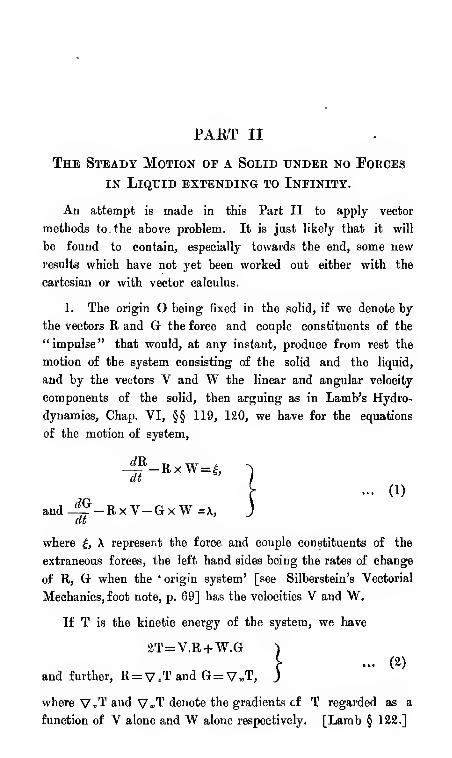
PART II
The Steady Motion oe a Solid tjndee no Forces
in Liquid extending to Infinity.
An attempt is made in this Part II to apply vector
methods to the above problem. It is just likely that it will
be found to contain, especially towards the end, some new
results which have not yet been worked out either with the
cartesian or with vector calculus.
1. The origin O being fixed in the solid, if we denote by
the vectors R and G the force and couple constituents of the
" impulse " that would, at any instant, produce from rest the
motion of the system consisting of the solid and the liquid,
and by the vectors V and W the linear and angular velocity
components of the solid, then arguing as in Lamb's Hydro-
dynamics, Chap. VI, §§ 119, 120, we have for the equations
of the motion of system,
-f-BxW=fc
and-^-RxV-GxW=X,at
(1)
where £, X represent the force and couple constituents of the
extraneous forces, the left hand sides being the rates of change
of R, G when the ' origin system' [see Silberstein's Vectorial
Mechanics, foot note, p. 69] has the velocities V and W.
If T is the kinetic energy of the system, we have
2T=V.R+W.G ^
and further, R= V „T and G= V „T, J
where V«T and V»T denote the gradients cf T regarded as a
function of V alone and W alone respectively. [Lamb § 122.]
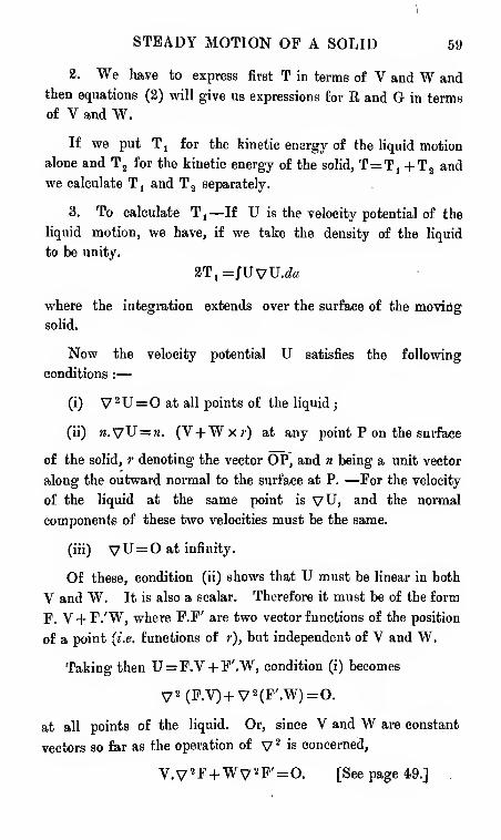
STEADY MOTION OF A SOLID 59
2. We have to express first T in terms of V and W andthen equations (2) will give us expressions for R and G in terms
of V and W.
If we put Tj for the kinetic energy of the liquid motion
alone and T 2 for the kinetic energy of the solid, T= T, +T2and
we calculate Ttand T 2 separately.
3. To calculate Tj—If U is the velocity potential of the
liquid motion, we have, if we take the density of the liquid
to be unity.
2T, =JUvUA
where the integration extends over the surface of the moving
solid.
»
Now the velocity potential U satisfies the following
conditions :
—
(i) V 2U=O at all points of the liquid
;
(ii) m.vU= k. (Y+Wxr) at any point P on the surface
of the solid, r denoting the vector OP, and n being a unit vector
along the outward normal to the surface at P. —For the velocity
of the liquid at the same point is VU, and the normal
components of these two velocities must be the same.
(iii) yU= at infinity.
Of these, condition (ii) shows that U must be linear in both
V and W. It is also a scalar. Therefore it must be of the form
F. V+F.'W, where F.F' are two vector functions of the position
of a point {i.e. functions of r), but independent of V and W.
Taking then U= F.V + F'.W, condition (i) becomes
V 2 (F.V) + V 2 (F'.W)=0.
at all points of the liquid. Or, since V and W are constant
vectors so far as the operation of V 2 is concerned,
V,V 8 F +WV 2 P'= 0, [See page 49.]
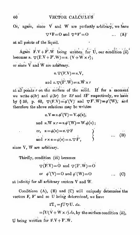
60 VE6TOR CALCULU^
Or, again, since V and W are perfectly arbitraryj we have
V 2F=Oand V 2 F'= ... (A)'
at all points of the liquid.
,.;,!• J
. h i.'i !,.,
.. -t £.. s. ., ill • ij I. -i
Again F.V+ F.W being written for U, our condition (ii)
becomes n. v(F.V+ F'.W)= ». (V+Wxr);
or since V and W are arbitrary.
*.V(F.V)=».V,
and «.v(F'.W)= «.'vv'x >
at all points r on the surface of the solid. If for a moment
we write 4>(Br) and i/f(8r) for 8F and 8F' respectively, we have
by §30, p. 40, V(F.V)= <£'(¥)' and vF'-W)=f(W)y and
therefore the above relations may be written
».V=».+'(V)=V.*(i0y
and m.W xr= w.i^'(W) =W.i/r(«)
;
or, n=<f>(n)=ri.'tfF
and rX(i=f()()=)i.VF',
(B)
since V, W are arbitrary.
Thirdly, condition (iii) becomes
V(F.V)=6 and v(F'.W) = 6'
or f(V) = Oaudf(W)= ... (C)
at infinity for all arbitrary vectors V and W.
. . • - j •.
• -.I
Conditions (A), (B) and (C) will uniquely determine the
vectors F, F' and so U being determined, we have
iiT1 =/UvU. da.
=JU( V+W x r).da, by the surface condition (ii),
U being written for F.V + F'.W.
STEADY MOTION OF A' SOLID 6l'
4. To calculate T 2 , the kinetic energy of the' solidf :—
We have, 2T 2=/(V+W
x
r). (V+ Wxr) dm, dm being an
element of mass of the solid at the point r and the integration
extending* through 'trie mas's:
of tn'e'moving :
solid:
That is, 2T 2= f[V.V+2V.Wx>-+ W. (rxWxr)] dm [see
p. 6].
=«» V.V + 8wlvVx W+.W.«(W)y
where m denotes the mass of the solid, r the vector to its
centre of gravity (so that fr dm=m r)y and m (W) has been
written for Jrx (Wxr)dm. Writing this integral in the form
f(r.rW—Wr.r)dm [p. 6], we seVtUstt' «' (W) is a self conjugate
linear vector function of W. Clearly also co(W) represents
what the angular momentum of the^ solid about O would have
been, , if Q had been fixed;- and W.<o(W) = constant, is;
for
variable W, -
the^ equation" of the" momenta! ellipsoid of the:
solid at O.
5. We can now writedown the expression for the' kinetic
energy of the system in terms of V and W. Thus,
2T=2T1-+2T 2
"
=/UVJa
+
JUW x r.da+ mY.V+ 2W?7V XW + W/»(-Wy:
For R° and 0,' then/ we calculate V»T a"nd" V»T from" this
expression for T. Noting tliat \j(a,:rf=d and' ^(r-4>r)=^/if 4 is self conjugate [p.' 28],' and that V„U= F aM V»U'= F',
we write down almost immediately
2 R= 2V„t=/Cji«+ VYJa+fH^xrJa+ tmY-f-imWxrand
2G=2v„f=/ F' V.tfa +j\Jrxda + f F'W x rJU+ Zm7 X V+ 2o.-(W).-
6. There are now certain relations among the integrals
occurring in these expressions for R and Gf. Justf to obtain*
these we prove generally that if V is any constant vector,
S S
JFV. (rf«.VF')=/F'.V(rfoVF),
62 VECTOR CALCULUS
F, F' being any two vector functions, satisfying v ! F= and
V*F'= at all points within the closed surface S over which the
integrations are performed.
If we put, as before, 8 F=<j>(Sr) and SF'= i/-(Sr), then da.yF'
=\}i(da) and da.^F=^>{da). If then Cis any arbitrary constant
vector
S SC./FV. (<to.vI")=jF.CTVX<fa)
S
=JF.(ty'(V).A»
s=/F.Cv(F'V).«fe.
Twhich by Green's Theorem =/V.[F.CV (F'.V)] dr, the volume
integral being taken through the volume T enclosed by S.
Using now (i) § 30, p. 38, and the relation v 2 F'= 0, we have
S TC./FV. (da.vI")=/V(F.O). V(F'.V) dr;
S TSimilarly, C./F'.V (<fe.vF)=JV(F.C).v(F'.V)rfr.
C being arbitrary, this proves our theorem.
In the application of this theorem to our problem, we have
to note that the region of integration would be that between
the surface of the solid and a sphere of infinite radius, and the
question of convergence of the integrals would arise. This
question has been discussed by Leathern in "Volume and Surface
Integrals used in Physics," Sections IX and XI.
7. Using this theorem now and remembering our surface
condition (B),««., <j>(da)= da and ty(da)=rxda) we have, among
the integrals in the expressions for R and G in § 5
JFV. da
=
JFV. tfda) =/F.V^(da)=JF.V da, ... (a)
jFWxr. da = JFW. rxda = /FW. tfda) = JF'.W <f>(da)
=JF.W<fa, ... (0)
STEADY MOTION OF A SOLID 63
/F'V. <to=/F'V.*(<fo) =/F.V^«)=/F.V? x rffl, ... (y)
jF'Wxjvfa = fWW.rxda = JF'W. ^ (<fa)= F'/W <\>{da)
=^F'.Wrxda ...(»)
Hence those same expressions for R and G may be written
R =j\Jda+mV +mWxr= [fF.Yda+ m\] + [fF'.Wda+mW x r],
G=JU»'x*+%xV+ u(W)= [/F.Vrx&+*xV]
+ [/F'.Wrxrf/ + o>(W)].
We write now R= $ 1V+ ^ aW, where <£„ <£ a are the two
linear vector functions,
<]>1Y=fF.Yda + mY
and <f> 2 W =jF'.Wda+mW xr.
Since the conjugate of a. r b is a r. b, (a) shews that $ x is
self conjugate. The conjugate of <£ aW=[F'W.da-mWxr
=jF.Wr x da+ mr x W, by (y),
so tbat<f>' 2Y=fF.Yrxda + mrX V. Hence we may write
G=4,' sV+ </. sW,
where <£„W = JF'."W> x rfo+ a>(W). Since a>(W) is self conjugate
(p. 78), (8) shows that <£ 3 is self conjugate.
Thus we may write
R=^V+^W
I(3)
and G =^V+ 3W.
where 4>\> <£„ are self conjugate functions.
This fact alone,—of <}> 1 , «£ 3 being self conjugate and </> a and
<t>'„ being conjugate—could of course be deduced directly from
(2), p. 74.
8. Considering now the case where no extraneous forces are
present, we have, putting £, A.=0 in equations (1) of page 74.
64, VECTOR CALCULUS
iR=RxW,
and i^=RxV+GxW.
The three well known integrals follow immediately.
(i) Multiplying the first equation scalarly by R, we have
R. *& =;,(,lj,fiW)=
.*. R.R = constant.
(ii) G.J-5 + R. -§ = (GRW) + (RRV) + (RGW)=a< »f •.'-"-
.-. R. G= constant.
R OThat is, the pitch of the wrench (Rj,G)
;which is^4^ is constant.
ti y nAgain, if r= , which we know is the perp. from O
on the a;xjs of. the wrench (R,G),
dr 1 r<#R „ , t. <2G na*o [^r-xG+Rx-r ]
= A, KR *W ) x G +.R x (R x V) + R xt(G xJf)]
,
XV. XV
which by the last formula of p. 6, reduces to
1
R.H[(R x G) xW+ R x (R x V)],
that is, *=rxW-V,
where V, =— Jr—j—
' = component of V perpendicular
to R.
STEADY MOTION OF A SOLID 66
If then (—Jdenote the rate of change of r in space, (—
)
"i_, 'xW+V=V"Vl=V" where V
«denotes the ex-
ponent of V parallel to R, i.e., to the axis of the wrench (R,G).
It follows that this axis is a fixed line in space, its direction
being obviously constant from the first of the equations of
motion.
But there was no special point deducing these results from
the equations of motion, as the fact they express, viz., the
constancy of wrench (R,G) in case no extraneous forces act,
was obvious a priori from the theorem that "the 'impulse' of
the motion (in Lord Kelvin's sense) at time t differs from the
impulse at time t„ by the time-integral of the extraneous forces
acting on the solid during the interval i— f"—[Lamb § 119]
—
of which theorem it is only an analytical expression that we have
in the equations of motion.
(iii) v 2T= R.V + G.W,
At At At At at
Using (3) P . 81, R-f + G.^reduces to V.f +W.f
•fIl =V.— +W. — =(VRW) + (WRV)At At At
+ (WGW)=
.'. T== constant.
9. These three integrals however are not sufficient to
determine the motion completely. We require three more scalar
60 VECTOR CALCULUS
(or one vector) integrals for determining the two vectors V and
W. The difficulty of finding them is avoided in two cases :
—
(i) When R=0, in which case we can utilise the known
solution of Poinsot in Rigid Dynamics.
(ii) Steady motion, when —— =0 and —— =0. so that tv ' J
dt dt
is got rid of altogether from our equations of motion.
10. The case R=0, is fully worked out in Lamb's Hydro-
dynamics, § 125. It may be interesting, just by the way, to
put the solution in vector form.
The equations of motion reduce, when R= 0, to
^ =GxW.dt
Again, putting R= in equations (3) p. 81,
we have V=-^ 1^W,
Now <j> 3 is self conjugate. Also, the conjugate of a 'product'
of linear vector functions being the ' product' of their conjugates
taken in the opposite order (Gibbs' Vector Analysis, Chap. V,
p. 295), and further <f>i al>d therefore fa1 also being self
conjugate, the conjugate of ^'j^T1^ is itself. That is, G is a
self conjugate linear vector function of W.
Hence, G=| V,„ (G.W) [see p. 28.]
It follows that Poinsofs solution is applicable.
11. But the case of steady motion does not seem to have
received yet the attention it deserves. Two simple particular
cases are well known—the permanent translation and the
permanent screws that we have when R= 0. It is proposed to
have a general investigation of the question here.
T ~ dY j dW , ,, dR n j dG n AIf —-— and ——are both zero, -^— =0 and —- =0, and our
dt dt dt dt
STEADY MOTION OF A SOLID 67
equations of motion of page 82 reduce to
RxW= ^)
[... (4)
andRxV +GxW = )
The first equation shows that R is parallel to W, or
R=— *'W, where # is a scalar. Substituting in the second,
we have
Again, putting R= —xW in equations (3), p. 81, we have
V=-**7iW-*l 1
* IW, ... (5)
and G=-^' 2^ 1W-</»'^7 1<^ 2W + ^» 3W.
Therefore,-(arV + G)= * lfl 1W + jrf,W + fl,W=OW >
where, 61= <f,-\ t=4,-*4>,+4>'
t4>-\ fl, = *'
1^7I*,-*„
and O has been written for the linear vector function
We have, then, nWxW= 0j ... (6)
and our conclusion is that in any case of steady motion W should
be parallel to OW.
12. By the rule for the conjugate of a product of linear
vector functions quoted in § 10, we see immediately that 1) 2 , 6 3
and therefore O also are self conjugate linear vector functions.
We recall now Hamilton's theorem of the latent cubic of a
linear vector functions.—In general, for any linear vector
function <f>, there are three vectors, say \1 , X 2 , A. 3 , of which the
directions are left unaltered by the operation of that function.
If ffi> 9%t 9s are the roots of the cubic equation
ff3 —m"ff a + m'g—m—Q,
where -=*-^f . * = \.^ y
J>
and^S^y^
68 VECTOR CALCULUS
a, /3, y being any three arbitrary non-coplanar vectors, then,
•Mi^Au ^2=^2^2 and <£A. 3 =<7 3A
3 . The cubic in g is
Called the latent cubic of <j>, and its roots the latent roots, and
the vectors X 1) A.2 , A 3 which retain their old directions after the
operation of <£ are called the axes of <£. If <j> is self conjugate,
the latent roots are all real, and the three axes real and mutually
perpendicular. [ Killand and Tait's Quaternions, Chap X.]
.
Applying this theorem, we conclude that for. any x there are
three mutually perpendicular directions for W, corresponding to
any one of which we may have a case of steady motion.
Further, if y is the latent root of O corresponding to the
axis W, OW=/W, and we have aV+G= — yW, or
G=—cV-jrW.
Thus our impulse is given by
R=-,<W )
... (7)
and G=-a-V-jrW. )
13. To construct a screw, therefore, such that the corres-
ponding motion of the solid may be steady, we find an axis
of the linear vector function il(r) corresponding to any x and
take W along this axis. V then is given by (5), p. 85 to
Wx Vbe —^7 aW— <j}- l
<j>fiW, Draw the vector———and through
its extremity draw a line parallel to W. This line is the
axis of the screw. If then the motion is started by the
impulse R = — ,rW and G= — 'V—$W, the solid will continue
to have the steady twist on our screw, the angular velocity
W.Vbeing W and the pitch WW
It is easily seen the axis of any screw and the axis of the
corresponding wrench coincide. For these axis being parallel
to W and R respectively are themselves parallel. Further,
. RxG -^Wxf-jV-yW) WxV ,, rS,DCe'Tnr=
(-»W).(-,W)=W these hnes are
STEADY MOTION OF A SOLID 69
drawn through the same point, so that the lines coincide and
either line is fixed in space.
If ji, p' denotes the pitches of the screw and wrench
(R.G) respectively,
KG _ -,tfW .(-. eV -yW) _ y* R.R (.cM').(-*W) ^"%
14. We conclude then that any x being specified, three
mutually perpendicular (though not necessarily intersecting)
screws of steady motion are determinate, except only as to the
magnitude of W ; and again that, by varying ,r, the directions
of screws of all possible steady motions would be obtained by
solving the vector equation n(>) x ;= (), or (a:,'0
1 r+ a0,/+ sr)
xi-0, in other words, by finding an axis of the linear vector
function 12.
It would be interesting now to enquire to what values of x
correspond the two cases mentioned in § 11, viz., permanent
translation and steady motion with R= 0.
Since, in any case, R= — .uW and W is not supposed to be
infinite, R= would make ,c= 0. O now reduces to 63 ,
G=-yW=-0 3W, V=-*7^W.
Since, again, when the motion of the solid is one of
translation only, W = and the screw reduces to V only; and
since, in any case, R is supposed to be finite, we see that in this
ease x tends to infinity in such a manner that ieW=-R,The equations (6) of p. 86, being written
(, t« 1W+ «1wAw)xR=0)
x
we see that in this case XR x R= 0, i.e. ^ 1RxR=0,
Hence the axis of the wrench, and therefore the axis of the
screw also is parallel to r, where r satisfies <£7'r x r= 0. That is,
V is parallel to an axis of fa1 or to an axis of $„ since ^ and
<£7l are co-axial.
?6 VECTOR CALCULI^
These permanent translations, of course, could be worked
out more directly by putting W= in (4>) of p. 85 and (3) of
p. 81.
15. If we eliminate x from
we shall obtain the whole assemblage of lines, to one of which
the axis of the screw corresponding to any case of steady motion
must be parallel.
Multiplying scalarly by 6xr and 6 a r respectively, we have
.i61 r.e irxr+e i
r.6 3rxr= 0,
and .b'i d
l ?:6 1rxr+ e i r.e srxr=0.
. r6 3r.6
rrxrl * _ 6
ir.6 arxr
"le^.e^xrJ O^.e^rxr
or, (B^fi^rxr) (0 i r.6 3rxr)= (0 !ir.6 1rxry,
which is homogeneous and of the sixth degre° in the tensor
of r, and represents therefore a cone of the sixth order, to some
generator of which the axis of every steady screw must be
parallel.
Obviously, the axes of the linear vector functions 6^ and a)
—which we came across as giving the directions of screws for
the special cases, § 14,—all lie on this cone, for the equation is
identically satisfied if we put either 6^r x r=Q or B\ x r= 0.
16. The motion of the solid being thus a twist about a
screw of which the axis is fixed in space and pitch constant,
it is almost obvious that each individual point of the solid would
be describing a helix about the fixed axis of the screw and
having the same pitch p (except of course points on the axis
which would move along the axis). For, if referred to a fixed
origin O' on the axis, the position of any point P of the solid
is specified by r,(0'J?=r))the velocity of P is—-=»W-fWx r.
at
STEADY MOTION OF A SOLID 71
Henee, (W x r)J-(Wxr)=Wx r. (Wx$)=Wxr.at at
[Wx(Wxr)] =
which shows that (Wxr).(Wxr) is constant, or the magnitude
of Wxr is constant. That is, the distance PN of P from the
axis of W is constant.
drThe formula for —shows, moreover, that the velocity parallel
at
to W is jbW, and velocity in plane perpendicular to W is W x r
so that the motion in this plane is instantaneously in a circle
(of which the centre is N and radius NP) with angular
velocity|W
|. Hence P moves in a helix of which the
piteh =fwr"
=p '
17. For the maintenance of a motion of this type, appro-
priate forces must be continuously acting on the solid, for weknow that the only motion a solid is capable of under no forces
is either one of uniform translation, or a uniform translation
combined with a motion of rotation about a principal axis of
the solid at the centre of gravity. We shall just verify that
fluid presssures exert on the solid just the force and couple
necessary for the maintenance of the sort of motion that we
have here.
Considering the general case (where the motion is not
necessarily steady), let $', \' denote the force and couple which
the fluid pressures on the solid are equivalent to. The linear
and angular moments of the solid are respectively
R 8=jH(V +Wxr) and G i =mr x V+ <o(W), ... (8)
72 VECTOR CALCULUS
these being just the terms of R and G that are obtained from T2
by the operation of V, and V« respectively. For the solid
alone, therefore, the equations of motion are
(It
and ~* = R 2 xV+ G 2 xW+ X'.
dt
If we further put now R-L =fTJda and Gi = J"U/x da, we have
R=R 1 +R S , G=G1 + G 2 . From our equations of motion
therefore of p. 32, we have
^l =R,xW-r and^ =R1xV+ G 1
xW—X'
dt at
Hence, £'=-% + R x xW and X'=-^iat at
+ R 1xV+ G
1xW.
JOConsidering steady motion now, for which-—
-
1- =0 andat
^i=0,wehavedt
f'=R 1x W and X'= R
tx V + G
x x W,
or, using (4) p. 85.
f=—R.xWand X'=-R2x V-G
2x W.
These formulae, for the special case of steady motion, could
of course be obtained directly by putting—-i = and —?. =at dt
in the equations of motion of the solid above.
Substituting now the values of R 2 , G 2 given in (8), we
obtain after slight reductions,
and X'= «(VxW)x;-w(W)xW,
STEADY MOTION OF A SOLID 73
If, again, we refer the motion to the centre of gravity of
the body as origin, so that r= 0, we have
( - (9)
where a>(W) now is the angular momentum of the solid about
its centre of gravity.
We notice that £' and X' both vanish only if either
(i) W=0, or (ii) V, W and to(W) are collinear. The first is
the case of one of the three permanent translations. In the
second case, since W and <o(W) have the same direction, "W is
along an axis of the linear vector function w, i.e., along a
principal axis of the solid at its centre of gravity. The axis
of the screw therefore is a principal axis of the solid at its
centre of gravity. These two, of course, are precisely the cases
in which we expected a priori that £', X' should vanish.
We show now that in the general case I', X' of formula
(9) are just the force and couple that would make the solid
continue to have its screw motion represented by V, W at the
centre of gravity. Since the motion of the centre of gravity and
the rotation of the solid about the axis W at its centre of gravity
can be considered independently, we show that the velocity Vof the C.G. is maintained by £', and then, regarding now the C.G.
at rest, that the rotation W by itself is maintained by X' ; or,
w,hat comes to the same thing, that the mass-acceleration of the
C.G. is equal to $' and that the rate of change of angular
momentum about c.s. is equal to X'.
For, if referred to a fixed origin O' on the fixed axis of the
screw, the position of the C.G:. is specified by r, then its velocity
dt
=jBW + Wxr,
™ =Wx* =WxV, V ^ =0,t= 0;dt dt at at
10
74 VECTOR CALCULUS
,•, m -— =)»WxV. which is our £'.
at
Again, the angular momentum of the solid about the C.Gr.
is <o(W), and in calculating its rate of change we take the C.G.,
which is now supposed to be at rest, as our origin. Since the
" origin system" [see Silberstein's foot note cited on p. 74] is
fixed in the body and rotates with it with angular velocity W,
the rate of change in question = -~—' — <d(W) xW(It
=Wx w(W), [V ™ =0],
which is our X'.
18. Having thus considered the general character of steady
motion in the preceding articles 11-17, we would next turn our
attention to the question of stability of these steady motions.
Before considering this question, however, it would be convenient
to summarise here a few propositions on the linear vector function
which we shall presently have occasion to use. The more
important ones are taken directly from Kelland and Tait's
Quaternions, Chap. X.
(i) From the well-known relation
r(a/3y)= (r/Jy)a+ (rya)P+ (fafly,
it follows easily enough, — say, by writing <}>(r) in the form
kr+a.r6 + cx r of page 24—that
(a0y)+to=WWW + (>7")<K/*) + (*»0)*(y).
Here a,/8,y are any three arbitrary non-coplanar vectors, and r
any fourth vector, and <£ denotes a linear vector function, (a/fy)
etc. of course, as explained on p. 6 stand for a./Jxy, etc.
(ii) For inverting the function <(,(>•) we have, if we denote
the inverse function by <£_1
,
m<j>~r(\ x fi.)
=
<£'A x $'/Uj
STEADY MOTION Otf A SOLID 75
where m(a/?y)= (^cK^y), and A., /x any two vectors.
If we introduce the function ^ by the definition,
<A(Xx/*)=<£'Xx<£y,
we may write symbolically m<fr 1 = \{r.
(iii) For inverting <j>r+gr, or {4>+g)r, where g is a constant
scalar, we have
(w +^+wV+^fo+^-'CXxfO-ft'+^Xx (*'+£>
where m, m', m" have the values defined on p. 86, viz.
m(apy)= {<H>P<h), m'Wy)= SH/tyy), »>0y) = 2(/3y<£a),' andthe function x is defined by
X(lx.p)=<t>'\.x fi+\.x<l>'fi..
(iv) Integrating <j>r over the surface of a parallelopiped of
which the edges are the vectors a,/3,y we get easily enough
!<l>rJ<r=2(Py<j>a).
Hence our m"= J,
'. =scalar constant of <j>
(aPy)
(v) We have also for any vector X.
w"X=c£X+ xX,
or, symbollically, m"=<A+x-
(vi) We already enunciated Hamilton's theorem of the
latent cubic on page 86. We only note here that if for any
function </>, m=0, the product of the three roots g x , g 2 and^ 3
of the latent cubic vanishes and therefore one of the roots, say
g 1} is zero. It follows that for such a function there exists a
vector Xj such that ^ 1 =0. Conversely, if for a function $ we
can find a vector Xtsuch that <j>\ 1 =0, m for that function must
vanish
76 VECTOR CALCULUS
Keeping to Gibbs' notation, we shall speak of m for any
function<f>
as its determinant and denote it by| <f> |
.
(vii) About the determinants of linear vector functions,
we have the theorems that the determinant of a ' product ' of
linear vector functions is the product of their determinants, and
that the determinant of the ' quotient ' of two linear vector
functions is the quotient of their determinants. Thus the
determinant of ^ 1^ I^»=iliU *s_L =_^?
, if «,,»„*,
are the determinants of <£ 1; <£ a , <j> s respectively. [See Gibbs,
p. 31 a.]
(viii) The inverse of the ' product ' of any number of
linear vector functions is the ' product ' of their inverses taken
in the opposite order. [Gibbs, p. 293]. Thus the inverse
of m,*,^*,*,)- 1^; 1*;
1*!
1.
19. To examine now the stability of any particular mode
of steady motion, we consider as usual the effect of a small
disturbance given to the system. V, "W being the linear and
angular velocities of the solid for the steady motion, and R, Gthe corresponding impulse, if 8V, 8W are the additional linear
and angular velocities imparted to the solid by the disturbance,
the total impulse that would generate from rest the new
disturbed motion is represented by
R + 8R=</>1(V + 8V) -H> 2(W + SW)
and G + SG=</>\(V+ 8V) + 4, 3(W+ 8W),
so that 8R=^ 1(SV) + <#» a
(8W)
and 3G=4>' 2 (8V)+</. 3(8W).
Our equations of motion of p. 82 now are
-^(R+ 8R)=(R+ 8R)xW + 8W)(it
andi(G + 8G)= (R+ 8R)x(V+SV) + (G + SG)x(W+ 8W),at
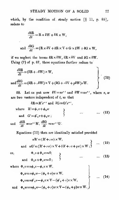
STEADY MOTION OF A SOLID 77
which, by the condition of steady motion [§ 11, p. 85],
reduce to
d8R
dt
dSG
=Rx8W + SRxW,
= (Rx8V +8RxV+ GxSW + 8GxW,dt
if we neglect the terms 8Rx8W, 8Rx8V and 8Gx8W.Using (7) of p. 87, these equations further reduce to
dmdt
,d8G
=(8R+ .,8W)xW,
and^ =(SR+ ,i8W) x V +(8G + .»8V +y8W)^W.dt
20. Let us put now SV=vent and $W=we"are two vectors independent of t, so that
SR=RV and SG=GV (
,
where B,'=<j>.lv+ <f> 1
w
and G'=c£'a «j+<£ sw ;
and —— =»e K, —— =ne" 'G.dt dt
Equations (10) then are identically satisfied provided
wR'= (R'+ jm>)xW, .
and tiG,=(E'+ w)xY+(G'+,ni+j«!).xV;i
or, <l>1u+ <t> aw=0,
and $,«+$,(«:
where &1v=n<f> 1 v—<{> 1vxW,
$ aM>=w<£ aw— (<£ a + x)w X W,
and &iw=n<f> !iw— (<t> 3 + x)w XV— (<£„ +y)w xW.J
(10)
where vsw
... (ii)
<,=0, ,
;=0; )
Y
(12)
(13)
(14)
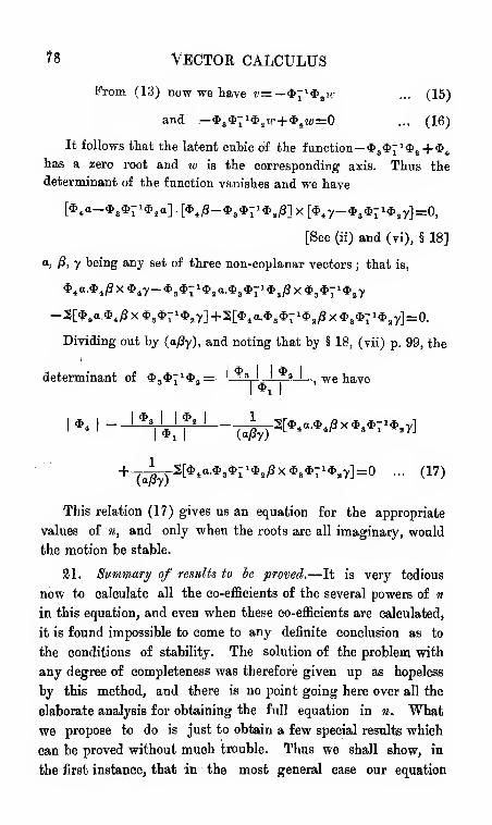
78 VECTOR CALCULUS
From (13) now we have v=—$-*$tiv ... (15)
and —$3$7 1$ a ?c+$ 4!w=0 ... (16)
It follows that the latent cubic of the function—
*
s*71*,+*
4i
has a zero root and w is the corresponding axis. Thus the
determinant of the function vanishes and we have
[See (ii) and (vi), § 18]
a, /?, y being any set of three non-coplanar vectors ; that is,
*4a.*10X* 1y-* s*71 *,a.*
1(
$7i*!Bj8x$,*7 1*
1,y
-2[*1a.*4^X$ 3*71*
2y]+2[* 1 a.* 3$71$
aj8x*3$7 1$ay]=0.
Dividing out by (a/3y), and noting that by § 18, (vii) p. 99, the
determinant of $ 3$71 4>
a=_LiJ
—
' * '
, we have
+7^yTs^ a '$3$Tl$^ >< *s$71$a '
)/]:=0 - (17)
This relation (17) gives us an equation for the appropriate
values of n, and only when the roofs are all imaginary, would
the motion be stable.
21. Summary of results to be proved.—It is very tedious
now to calculate all the co-efficients of the several powers of w
in this equation, and even when these co-efficients are calculated,
it is found impossible to come to any definite conclusion as to
the conditions of stability. The solution of the problem with
any degree of completeness was therefore given up as hopeless
by this method, and there is no point going here over all the
elaborate analysis for obtaining the full equation in n* What
we propose to do is just to obtain a few special results which
can be proved without much trouble. Thus we shall show, in
the first instance, that in the most general case our equation
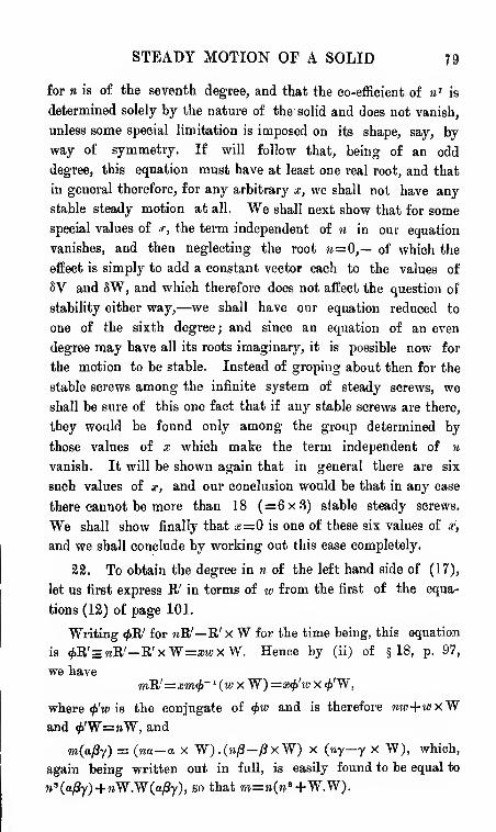
STEADY MOTION OF A SOLID 79
for n is of the seventh degree, and that the co-efficient of n 1is
determined solely by the nature of the solid and does not vanish,
unless some special limitation is imposed on its shape, say, by
way of symmetry. If will follow that, being of an odd
degree, this equation must have at least one real root, and that
in general therefore, for any arbitrary x, we shall not have any
stable steady motion at all. We shall next show that for some
special values of x, the term independent of n in our equation
vanishes, and then neglecting the root n=0,— of which the
effect is simply to add a constant vector each to the values of
§V and SW, and which therefore does not affect the question of
stability either way,—we shall have our equation reduced to
one of the sixth degree; and since an equation of an even
degree may have all its roots imaginary, it is possible now for
the motion to be stable. Instead of groping about then for the
stable screws among the infinite system of steady screws, we
shall be sure of this one fact that if any stable screws are there,
they would be found only among the group determined by
those values of x which make the term independent of »
vanish. It will be shown again that in general there are six
such values of se, and our conclusion would be that in any case
there cannot be more than 18 (=6x3) stable steady screws.
We shall show finally that x=0 is one of these six values of x,
and we shall conclude by working out this case completely.
22. To obtain the degree in n of the left hand side of (17),
let us first express B/ in terms of w from the first of the equa-
tions (12) of page 101.
Writing <£R' for mR'—R' xW for the time being, this equation
is ^R'=TOR'-R'xW=a;wxW. Hence by (ii) of §18, p. 97,
we havewE'rmf 1 (w x W) =%<t>'w x 4>'W,
where <f>'w is the conjugate of <f>w and is therefore nw+wxWand <j>'W=riW, and
ra(a/fy) = (na—a X f).(»j3-|3xW) X (ny—y X W), which,
again being written out in full, is easily found to be equal to
n s (a/3y)+nW.W(a.Py), so that w=w(w a +W.W).
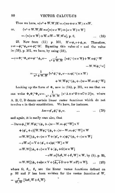
80 VECTOR CALCULUS
Thus we have, <«' +W.W)R'=,t(w+i« x W) x iiW,
or, (n*+W.W)R'=x[n(wxW) + (wxW)xW]
= i[n(wxW)+W.wW-W.Ww], p. 6, ... (18)
23. Now from (11) p. 101, R'=^ lV+ <l> t w. Therefore,
v=— <l>i1
<t> iw+<f>~1 R'. Equating this value of v and the value
in (15), p. 101, we have, by using (18),
=w»+w.w [^'B-»^'( |"'v )
fW.Wcfc l(<£ 2 + .!-)u>-W.wx^>7 lW]
Looking up the form of $ 3now in (14), p. 101, we see that we
can write &,&~ 1&„w= ^r^=r \n :sA+ n*~B+nC+ T)]w, where
A, B, C, D denote certain linear yector functions which do not
involve n in their constitution. We have, for instance.
A«=*' i^7^ I», ... ... (19)
and again, it is easily seen also, that
-Dw=^ 1[W.W^7 1(^2 + .«)u'-W.w^7 1WJxV
+ (£'a + xi)[W.W<l>1 1
(<j> t + x)w—W.w^~ lW] xW
=f.V[(^+.c)»xV+(^+%xW]
-BW.M>[2.c01W+0
aW] X W, by (5), p. 85,
=W.W[(^ +as)w x V+(^ +fi w+¥.wF) x W], ... (20)
where ii, lt a are the linear vector functions defined on
p. 86 and F has been written for the vector function of W,
STEADY MOTION OF A SOLID 81
24. Our2[*1a.*^x$ 3 <E.71*ay]of (17), p. 102, then, is of
the form
where »A'+B' has been written for <&4 , so that
A'a=<£s a, and -B'a=(^+s)axV+(^s +!()oxW.
Obviously A', B' also do not involve n. We may write therefore
W»+W.W t"" 5^ +a*w * +a 3»s +«»«* +«!»+«„]
where the a's are all independent of n. The values of a6
and a
may be written down immediately. Thus
(a^)a( =2[A,a.A^xAy]=2[^a.^^xfa^'^y], ... (21)
and (a0y)ao =2[B'a.B'i8xDy] ... (22)
25. Again, with the same notation,
= -m (n> +W.Wy SK-A'+ff)* (••A+.'B+^J+D)/!
x (M sA+»*B+M0+D)y],
which/is of form L. [a' 7w 7 +a'
fl» 6 +a 5»
5 + ... + a' ],
where also the co-efficients of the powers of n are independent of
«. Clearly also,
(a^y)a'7=2[A'a. A/?X Ay]=Sft s
a- <t>'^V<t>^
xVAV^y], ... (23)
and (a/Jr)a' =S[B'a. D^xDy] ... (24)
11
£2 VECTOR CALCULUS
26. We try to form an idea now of the other terms
|*
x | , |*
a |and
| $„ |that occur in (17), p, 102.
(i) We note in- the first instance that <j>(r) being any liner
vector function and a any constant vector, the determinant of
<£r x a vanishes. For,
((f>a x a), (</>/? X a) X (<£y X a) =[<£a X a]. a(<£/3<£ya) =0, [page 6.]
"It follows that the parts independent of n in $7r an^ *a r > v^z -'
-^,fxW and— (^ 1+.'")»'XW have their determinants equal to
zero.
(w) We note again that if <£,, $ s are any two linear vector
functions, the determinant of n^^+tfj^ is easily found by writing
out the expanded form of
(rfh)Kw*»a+ *» a)- OM+<M)x0W>iy+«£,y)],
to be «*!»»• +/M» , +/i,M+m a ,where m
l,m t are the determinants of
<t> 1 , 4> t respectively and >, //.' are determined from
and/(a/?y)=_2[^la. <£,/Jx<£,y]
It follows that, the terms independent of u vanish in both
| 4>! |and
|<E>
2 |. We find, in fact, by working out
[W.a-^axWM^.jS-f^xWjxW.y-fyxW)],(«0y)
as in § 22, that
|Q
l |=m
1»(»»+W.W),
where m, is the determinant of i^.
We may write also
| *, |=w,w 8 4-6,w , +c
!l«J

STEADY MOTION OF A SOLID 88
where ma
is the determinant of either ef the two conjugate
functions<f> 3 , •£', and m a is the determinant of
(f> s , and the b't, cV
and d's are all independent of n and in general none of them
vanishes,
27. For our equation in n then, corresponding to (17) p, 102,
we have
m.jw' + b in" +c in+di
_ (mtn* + b tn'+ c in+d a )(mt n'' + b tn+ c, )
_a tn*.+ ...+a.
+ o',« 7 + ...+o'.
=0. ... ... ... ... (25)
Multiplying out by (w ! +W.W) S, we get an equation of the
seventh degree in to.
The co-efficient of n'1
=to 3— a a + a'
7— —s.
to,
-I f.+T
1
*. I ,
by (21) p. 106 and (23) p. 107, and (vii), p. 99.
Remembering now theorem (ii), § 26, we see that this co-efficient
=| <t> a
—^'j^ 1^ j=—
|6 S | fii having the same definition
as on p. 86. Obviously, our co-efficient of n 7 does not vanish,
unless the functions<f> 1 , <j> 3 and
<f> a are given in special Ways,
unless, that is to say, some special restriction is imposed on
the shape of the moving solid, for these functions are solely
determined by the form of the bounding surface of the solid.
84 VECTOR CALCULUS
28. We may write down also the term independent of n in
the same equation. This term directly
=(W.W) , d4 -a.W.W+o' -W.W c-^
Now if, as in § 24, we write » A'+B' for $ 4 , d t by (ii) § 26 is
the determinant of B'. That is,
d4 (a0y)=(B'»B'/3B'y).
The values of a„, a' „ are given by (22) and (24), viz.,
(a]3y) a.=S[B'o. B',3xDy]=W.W2[B'a.B'0xD'y],
(a0y)a' o =2[B'a. D/3xDy]=(W.W) a S[B'a. D'jSxD'y],
if a new function D' is introduced by the definition
_DV= =L= Dr, which by (20) p. 106W.vv
=(^+ai)rxV+W s +fl)r+¥,rF]xW, 1
where F=—^^ P^W+fl.W]
Hence, (W.W) 2c?4 -a 11
W.W+o'(,
.(26)
=(WJW)f [(B'aB'/8B'y-S(B'aB')3D y) + S(B'aD')8D'y)]
(a/3y)
=(W.W)»[|B'-D'
| + |D'
| J, by (ii), § 26,
But (B'-D')r=[(0-y)r+W.rP] X W,
and, therefore, by (») § 26, |B'-D'
|=0.
Therefore, (W.W) sd1-a ()W.W+a'
1)=(W.W)« |"D'
|.
Hence our term independent of «
-W.W[W.W |D'
| -^-s
] = W.W[|D
| -^1 -. (27)
STEADY MOTION OF A SOLID 85
29. For further simplification of this term, we calculate
generally the determinant of
4> lt <f> t being any two linear vector functions.
Since the determinants of both ^yxY and <£ ayxW are zero
fey (*) § 26, the determinant in question is by (ii) § 26,
= * [2(<M x V). (<M x V) x (0 sy x W)(.o-py)
+2(^axV). (<MxW)x(4»>y xW)]
Now SOM xV)x(f|3x V).(<£ ay x W)
=2(^» 1a^ l/8V)V.(^ syxW)
=WxV.<i> i<K
lV(<t> 1 °i<t> i P<t>iy), by (i), § 18, p. 96
=Wx V. <£ s<£rV WtOjSy), m xbeing
| <£, | .
Again, S(^axV). (fapxW) x (^9yxW)
=2W 1axV).W(^^ 8yW)
=VxW.S[(^ a/8^yW)^ 1a]
=VxW. <MrW aa4> a /ty ay)
=VxW. ^^W ma (a/?y), m a being '
<£,|
The determinant of ^rxV+^xW is therefore
=WxV. [w^^V-m^^W] ... (iii)
=WxV. [<^ a^ 1V— <#>i"A aW], in the notation of (ii), p. 97
18.
30. Applying this result now, we easily calculate d?
and
ID' I,
86 VECTOR CALCULUS
Thus, if we write »A"+B" for *,, d tis by (ii), § 26 the deter-
minant of B". That is,
—d t=determinant of t^r XV+ (<£'
a + .p> XW=WxV. [(*'. + *Wi V-</. 1 (f a +.M 3
+*»)W], by
(iii) § 18, p. 97
Again,— | D' | = determinant of (<£ a+.r)rxV+/»-x "W,
[(26), p. 110]
if/ris written for the linear vector function (</>,+ 0)r+W.rF.
Hence, we have- | D' | =WxV. [/(</',+.c ,r,+.t;»)V
-(^, + xOsrW],
where ^ denotes the ^ function for/, that is,
* (ax/3) =/.x/i8 = [* 3 + fi) a+ W. Fa] x [4> 3 +0) £
+ W. F/3].
31. For the expression (27), c, only remains to be calcu-
lated. This is done directly. Thus by (ii), §. 26,
ca (a/Jy) = S^a. [(*,+*) /SxW^X^+.JyxW]
= S</>,«. W [(<*>,+*) )8x (*,+*) y. W]
= 2</>,a. W [(*»+*x'.+f .) 0x r)]. W, [see («¥), p. 97]
= S* aa. W [* (0yW) + * (XaW/2y) + (^WjSy)]
= W. [;C «2 (/JyW) *,a+ »2 (ar.WjSy)*, a
+2(^Wi8y)V»,a]
which by (»), §18 = (a/3y) W. [.e2</>, W+ ^,Xi W+ ot
2 W],
since by (ii), §18, ^^W = m^ W.
.'. c 2=^ 2 W. *, W + lC W. «£ sXsi W + m 3
W. W.
32. The term independent of n, then, in our equation for
w. is, as given in (27),
W. W [W. W | D' |_ c a 1
,
tnlJ
STEADY MOTION OF A SOLID 8?
where c2 , d~ and | D' | have the values calculated in the last
two articles. As explained in §21, it is necessary for stability
that this term should vanish. A necessary, — of course, not
sufficient — condition therefore that any one of the three steady
screws corresponding to .0 should be stable, is- that x should
satisfy W. W|D' |
- c& = ... ... (28)
Since now x occurs in the first degree in V [(5), p. 85], in
the second degree in O [p. 86] and F [(26), p. 110] and in the
fourth degree in g, it appears from an inspection of the values
of cf , d3 and
|D'
|given in the last two articles, that (28)
represents an equation of the sixth degree in ,c, and will, in
general, therefore determine only six values of o. No x other
than these six can possibly determine a stable steady screw.
33. We prove now that $= is always one of this set of
six values of .«. It is only necessary to show that (28) is satis-
fied when j; = 0.
For, when ,i;=0, the expression for —DV in (26), p. 110
reduces to
F being zero, and <£ 3+fl reducing to <£ 3 +0 3 , i.e. to «^'
a^» 1
_1*^
a
in this case. Hence now by (Hi), p. 112,
-|D'
|=WxV. [m, ^I^^V- j
<^'^-^2
.
|
But, by (vii) and (viii), §18,
mI ^T 1
*, I=~ and GMT 1*.)" 1 =*V*x#V-
Hence, - |D'
| = WxV. Kp-'V- —>- <M';*W]
= -?- Wx V " ^'^iV-^if 2W], by (it), §18.fit 1
VECTOR CALCULUS
Also, putting x= in the values of c 2 , d s in §§30, 31, we
and -d 3=WxY. |>' 8 tY-^ t
W\
have now c 2 = »* 2 W. W
It follows that W. W I D' I - C-^2 =0 identically whenm
l
x= 0.
34. Thus the case as= satisfies our necessary condition of
stability. It is a relevant enquiry then if any one of three
screws corresponding to this case is stable. This is the case
(§14) when the impulse producing; the original steady motion
reduces to a couple alone, G= — 3W= —yW ; R=0.
For equations (12) of p. 101, we write now
hR'=R'xW
»G'=R'xV+ (G'+yw) xW,
From the first, R'=0 (for no vector can be perpendicular to
itself), and therefore the second reduces to
»G'=(G'+p)xW ... ... (29)
Putting again R'=0 in (11) p. 101, we have
v = —fcifaw, G' = -f 8</>r^*+^ s «» = —6„w.
Writing </> for S for convenience, we have G'= — <l>to
or n<f>to— (<l>—y)wxW= 0. ... (30)
Putting the determinant of the function on the left hand
side of (30) to zero, we shall have our equation for the appro-
priate values of n in this case.
The determinant in question is, by (ii) § 26
m n 3 + bn* +cn + d,
STEADY MOHON OF A SOLID 80
where, —d= determinant of ( —y) wxW= 0, by («') § 26;
m = determinant of <£ =| 3 | ;
c=y 2W. fW-yW. <l>xW + mMV. W, fust as in the
calculation of c 2 in § 31
;
and — b (<*/3y) =S(^aX<^>/3). [<£—^)yxW], which we find to
be zero when we write it out and remember also that <£ is self
conjugate ; so that b= 0.
Hence, our equation for n now is
mn 3 + n [y2W. <f>W-yW. <t>xW + mW. W]=0 ... (31)
[We may note, by the way, here that the co-efficient of n 8
in this equation, viz., m or 3 |, is the same (but for the
sign) as the co-efficient of n 7 in the equation for n in the general
case (see §-
!7, p. 109). Since this last co-efficient in any case
is independent of x, and since equation (31) is only the reduced
form, when .r = 0, of the general seventh degree equation, we
see that when .i. = 0, not only does the term independent of it
vanish in the genera] equation, (as we have proved in § 33),
but the co-efficients of all terms from u 4 downwards vanish
too].
35. Now one root of equation (31) is m= 0, and the other
two are given by
»* = - —- |>2W. fW-yW. 4>\W +mW. W]
m
since 0W=/W, and by (V) § 18, \—m"— ^>, this simplifies to
*i = _ w - w[a*8-»«v + *]-
m
The motion is stable, therefore, if y is so chosen that
—L [2*» -«*>»+»] ... ... (32)m
is positive. Now, by Hamilton's theorem of the latent cubic,
(§ 12, p. 86) y may have any one of three values, viz., the roots,
say y t , y-i,ys> of the equation
y 8 — m"y 2 + m'y—m= 0,
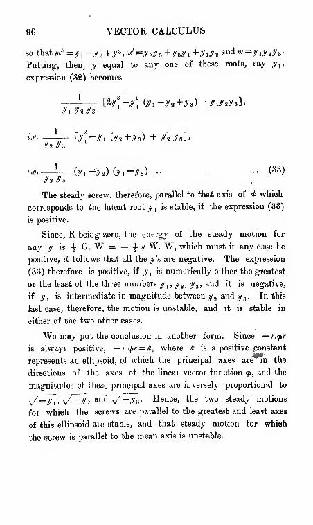
90 VECTOR CALCULUS
so that m"=yl +y t +y i ,>"'=y»y 3 +9s9i +2/^2 and»?=#,y 2y 8
.
Putting, then, y equal to any one of these roots, say y x ,
expression (32) becomes
— m\—i\ iSi+9t+9») -3fi9a3fa]'
i.e ii-Vx <Jt+9i) + 3f*l/a]>
i.e. -^—bi -*-*,) (3 1-*,) ••• •• (33 )
The steady screw, therefore, parallel to that axis of <£ which
corresponds to the latent root^ is stable, if the expression (33)
is positive.
Since, R being zero, the energy of the steady motion for
any y is \ G. W = — \ y W, W, which must in any case be
positive, it follows that all the y's are negative. The expression
(33) therefore is positive, if y, is numerically either the greatest
or the least of the three numbers y t , y 2 , y 3 , and it is negative,
if y xis intermediate in magnitude between y 2
and ^3. In this
last case, therefore, the motion is unstable, and it is stable in
either of the two other cases.
We may put the conclusion in another form. Since —r.$r
is always positive, —r.<f>r= k, where h is a positive constant
represents an ellipsoid, of which the principal axes are in the
directions of the axes of the linear vector function<f>, and the
magnitudes of these principal axes are inversely proportional to
*/—!/[, sj—y-2 and \/—y s . Hence, tl^ie two steady motions
for which the screws are parallel to the greatest and least axes
of this ellipsoid are stable, and that steady motion for which
the screw is parallel to the mean axis is unstable.