vector and affine math - university of texas at austinfussell/courses/cs354/lectures/...vector...

University of Texas at Austin CS354 - Computer Graphics Don Fussell

Vector and Affine Math

Don Fussell Computer Science Department

The University of Texas at Austin

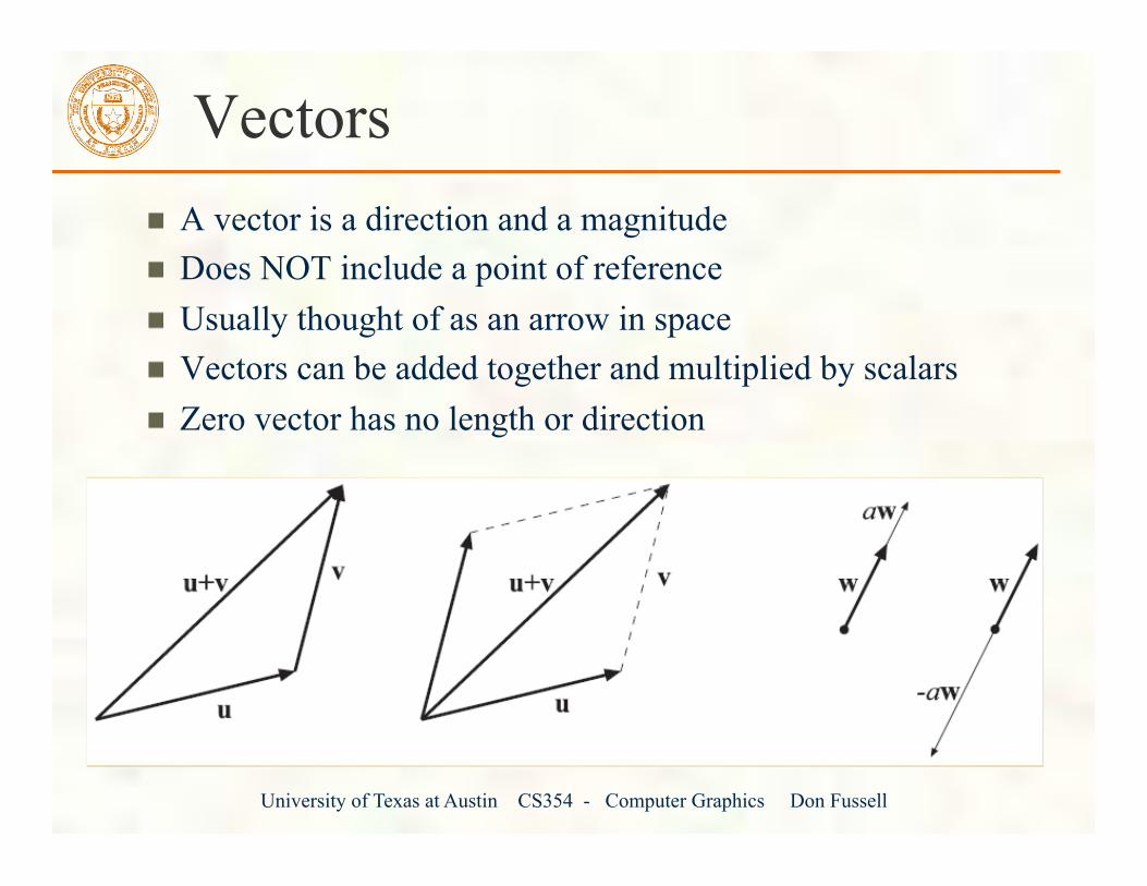
Vectors   A vector is a direction and a magnitude   Does NOT include a point of reference   Usually thought of as an arrow in space   Vectors can be added together and multiplied by scalars   Zero vector has no length or direction

Vectors


Vector Spaces   Set of vectors   Closed under the following operations

Vector addition: v1 + v2 = v3

Scalar multiplication: s v1 = v2

Linear combinations:

  Scalars come from some field F e.g. real or complex numbers

  Linear independence   Basis   Dimension

vv =∑=

i

n

iia

1



Vector Space Axioms  Vector addition is associative and commutative  Vector addition has a (unique) identity element (the 0 vector)  Each vector has an additive inverse

So we can define vector subtraction as adding an inverse

 Scalar multiplication has an identity element (1)  Scalar multiplication distributes over vector addition and field addition  Multiplications are compatible (a(bv)=(ab)v)


Coordinate Representation

 Pick a basis, order the vectors in it, then all vectors in the space can be represented as sequences of coordinates, i.e. coefficients of the basis vectors, in order.  Example:

Cartesian 3-space Basis: [i j k] Linear combination: xi + yj + zk Coordinate representation: [x y z]

][][][ 212121222111 bzazbyaybxaxzyxbzyxa +++=+


Row and Column Vectors

 We can represent a vector, v = (x,y), in the plane

as a column vector

as a row vector €

xy"

# $ %

& '

€

x y[ ]

Linear Transformations

 Given vector spaces V and W  A function is a linear map or linear transformation if


f :V→W

f (a1v1 +...+ amvm ) = a1 f (v1)+...+ am f (vm )


Transformation Representation

  We can represent a 2-D transformation M by a matrix

  If v is a column vector, M goes on the left:

  If v is a row vector, MT goes on the right:

  We will use column vectors.

v'= vMT

!x !y"#

$%= x y"

#$%

a cb d

"

#&

$

%'

v'=Mv

!x!y

"

#$$

%

&''= a b

c d

"

#$

%

&'

xy

"

#$$

%

&''

€

M =a bc d"

# $

%

& '


Two-dimensional transformations

 Here's all you get with a 2 x 2 transformation matrix M:

 So:

 We will develop some intimacy with the elements a, b, c, d…

€

" x " y

#

$ % &

' ( =

a bc d#

$ %

&

' (

xy#

$ % &

' (

€

" x = ax + by" y = cx + dy


Identity

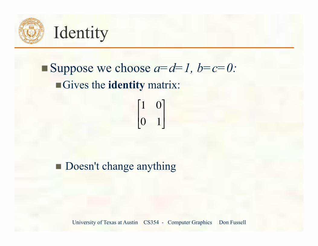
 Suppose we choose a=d=1, b=c=0: Gives the identity matrix:

Doesn't change anything €

1 00 1"

# $

%

& '


Scaling

  Suppose b=c=0, but let a and d take on any positive value: Gives a scaling matrix:

Provides differential (non-uniform) scaling in x and y:

€

a 00 d"

# $

%

& '

€

" x = ax" y = dy

€

2 00 2"

# $

%

& '

€

1 2 00 2

"

# $

%

& '

1

2

1 2

1

2

1 2

1

2

1 2

x

y

x

y

x

y


Reflection

 Suppose b=c=0, but let either a or d go negative.  Examples:

x

y

x

y

x

y

x

y

€

−1 00 1#

$ %

&

' (

€

1 00 −1#

$ %

&

' (


Shear

 Now leave a=d=1 and experiment with b  The matrix

gives: €

1 b0 1"

# $

%

& '

€

" x = x + by" y = y

1

1

1

1x

y

x

y

€

1 10 1"

# $

%

& '


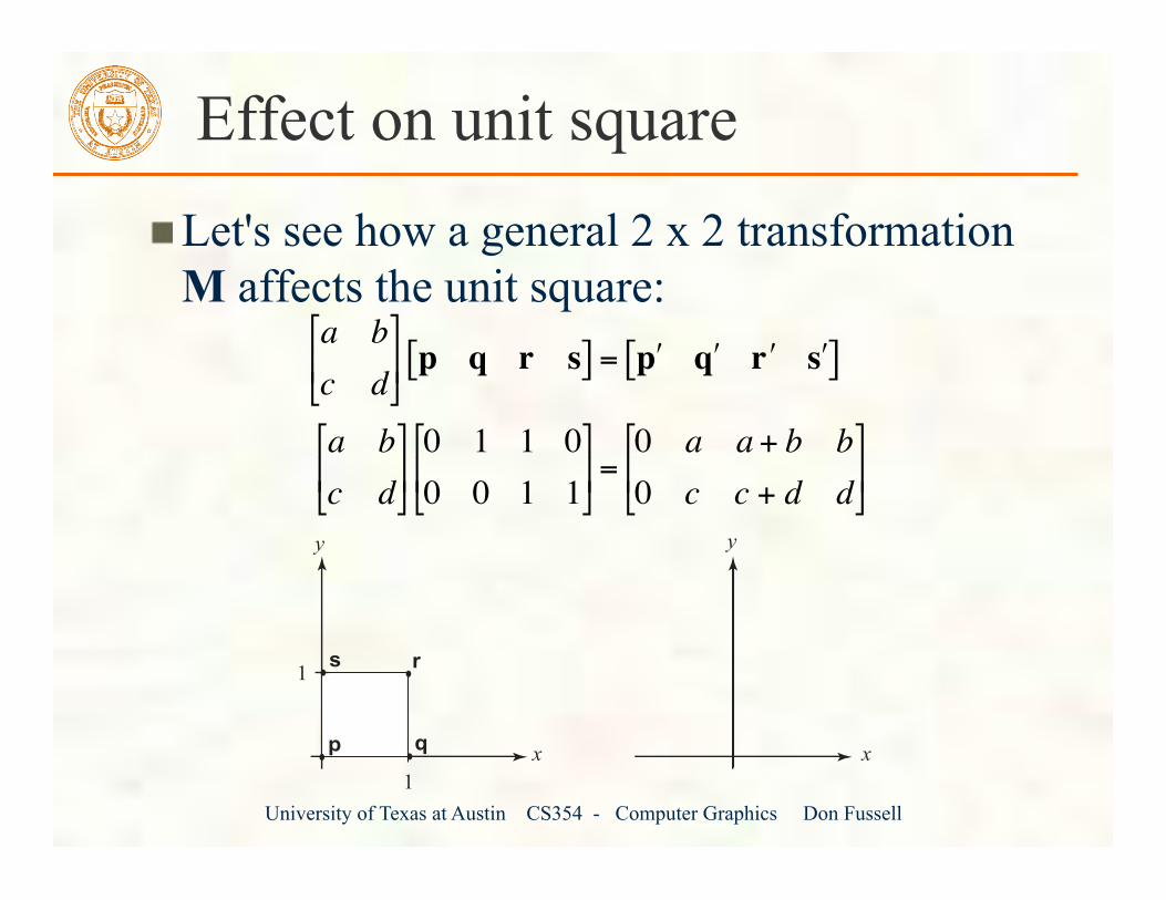
Effect on unit square  Let's see how a general 2 x 2 transformation M affects the unit square:

1

1

p q

rs

x

y

x

y

€

a bc d"

# $

%

& ' p q r s[ ] = ( p ( q ( r ( s [ ]

a bc d"

# $

%

& ' 0 1 1 00 0 1 1"

# $

%

& ' =

0 a a + b b0 c c + d d"

# $

%

& '


Effect on unit square, cont.

 Observe: Origin invariant under M M can be determined just by knowing how the corners (1,0) and (0,1) are mapped a and d give x- and y-scaling b and c give x- and y-shearing


Rotation

  From our observations of the effect on the unit square, it should be easy to write down a matrix for “rotation about the origin”:

Thus

1

1x

y

x

y

€

10"

# $ %

& ' →

cos(θ)sin(θ)"

# $

%

& '

01"

# $ %

& ' →

−sin(θ)cos(θ)"

# $

%

& '

€

MR = R(θ) =cos(θ) −sin(θ)sin(θ) cos(θ)$

% &

'

( )


Linear transformations   The unit square observations also tell us the 2x2 matrix transformation

implies that we are representing a vector in a new coordinate system:

  where u=[a c]T and w=[b d]T are vectors that define a new basis for a linear space.

  The transformation to this new basis (a.k.a., change of basis) is a linear transformation.

v'=Mv

= a bc d

!

"#

$

%&

xy

!

"##

$

%&&

= u w!"

$%

xy

!

"##

$

%&&

= x ⋅u+ y ⋅w


Limitations of the 2 x 2 matrix

 A 2 x 2 linear transformation matrix allows Scaling Rotation Reflection Shearing

  Q: What important operation does that leave out?

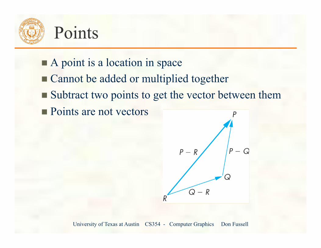
Points  A point is a location in space  Cannot be added or multiplied together  Subtract two points to get the vector between them  Points are not vectors


Points

• A point is a location in space

• Cannot be added or multiplied together

• Subtract two points to get the vector between them


Affine transformations

  In order to incorporate the idea that both the basis and the origin can change, we augment the linear space u, w with an origin t.   Note that while u and w are basis vectors, the origin t is a point.   We call u, w, and t (basis and origin) a frame for an affine space.   Then, we can represent a change of frame as:

  This change of frame is also known as an affine transformation.   How do we write an affine transformation with matrices?

!p = x ⋅u+ y ⋅w+ t

Basic Vector Arithmetic


u =rst

!

"

###

$

%

&&&v =

xyz

!

"

###

$

%

&&&u+ v =

r + xs+ yt + z

!

"

###

$

%

&&&

av =axayaz

!

"

###

$

%

&&&

v = x2 + y2 + z2 norm(v) = vv

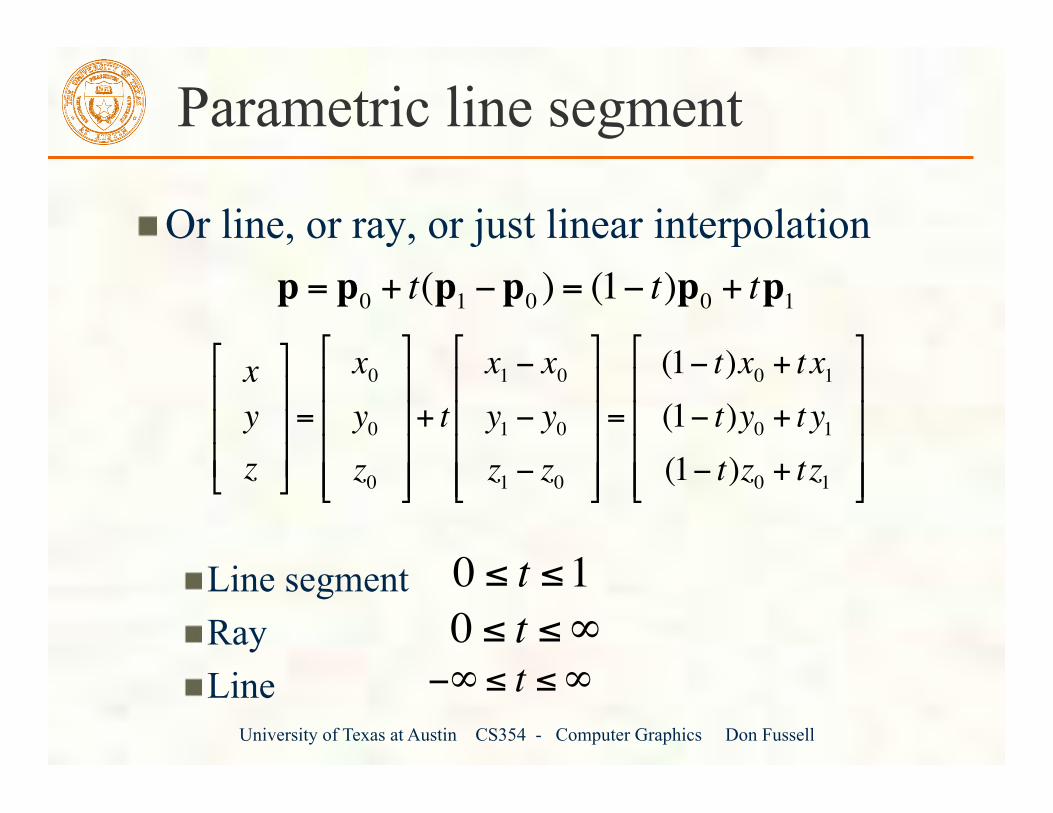
Parametric line segment

 Or line, or ray, or just linear interpolation

Line segment Ray Line


p = p0 + t(p1 −p0 ) = (1− t)p0 + tp1

xyz

!

"

###

$

%

&&&=

x0y0z0

!

"

####

$

%

&&&&

+ tx1 − x0y1 − y0z1 − z0

!

"

####

$

%

&&&&

=

(1− t)x0 + t x1(1− t)y0 + t y1(1− t)z0 + tz1

!

"

####

$

%

&&&&

0 ≤ t ≤10 ≤ t ≤∞−∞≤ t ≤∞

Vector dot product


u ⋅v = rx + sy+ tz = u v cos(φ)

Dot product

• Formula:

• Alternately:

• Where φ is the angle between the vectors

Projection

Projection (u component parallel to v)

Rejection (u component orthogonal to v) Particularly useful when vectors are normalized


Projection / rejection

• Projection:

• W is the part of U that lies on V

• Rejection: Just U - W

w = u ⋅vv ⋅v

v

u−w

Cross product intuition

• If U & V point along the same line, W = 0

• Useful for constructing local coordinate frames

• Length of cross product is area of parallelogram

spanned by U and V (divide by 2 for area of the

triangle)

Cross product

 w is orthogonal to u and v     area of parallelogram  use right-hand rule  


w = u× v =i j kr s tx y z

=

sz− tytx − rzry− sx

#

$

%%%

&

'

(((

Cross product

• Formula:

• Creates a vector that is:

• Perpendicular to the inputs

• Length

• Right-hand orientedw = u v sin(φ)w

u× v = −(v×u)(u× v)×w ≠ u× (v×w)

Determinants

det(MT) = det(M) det(AB) = det(A)det(B)  if det(M) = 0, M is singular, has no inverse


a bc d

= ad − bc

a b cd e fg h i

= a e fh i

− bd fg i

+ c d eg h

= aei− afh+ bfg− bdi+ cdh− ceg

Plane equation

 Given normal vector N orthogonal to the plane and any point p in the plane

 For a triangle  Order matters, usually CCW


N ⋅p+ d = 0

a b c!"

#$

xyz

!

"

%%%

#

$

&&&+ d = ax + by+ cz+ d = 0Triangle normals

• Every triangle lies in a plane

• 2 choices of normal, pick one by convention

• CCW winding is usually used

• Formula:

N = norm((v2 − v0 )× (v1 − v0 ))


Homogeneous Coordinates   To represent transformations among affine frames, we can loft the

problem up into 3-space, adding a third component to every point:

  Note that [a c 0]T and [b d 0]T represent vectors and [tx ty 1]T, [x y 1]T and [x' y' 1]T represent points.

!p =Mp

=

a b txc d ty0 0 1

"

#

$$$$

%

&

''''

xy1

"

#

$$$

%

&

'''

= u w t"#

%&

xy1

"

#

$$$

%

&

'''

= x ⋅u+ y ⋅w+1⋅ t


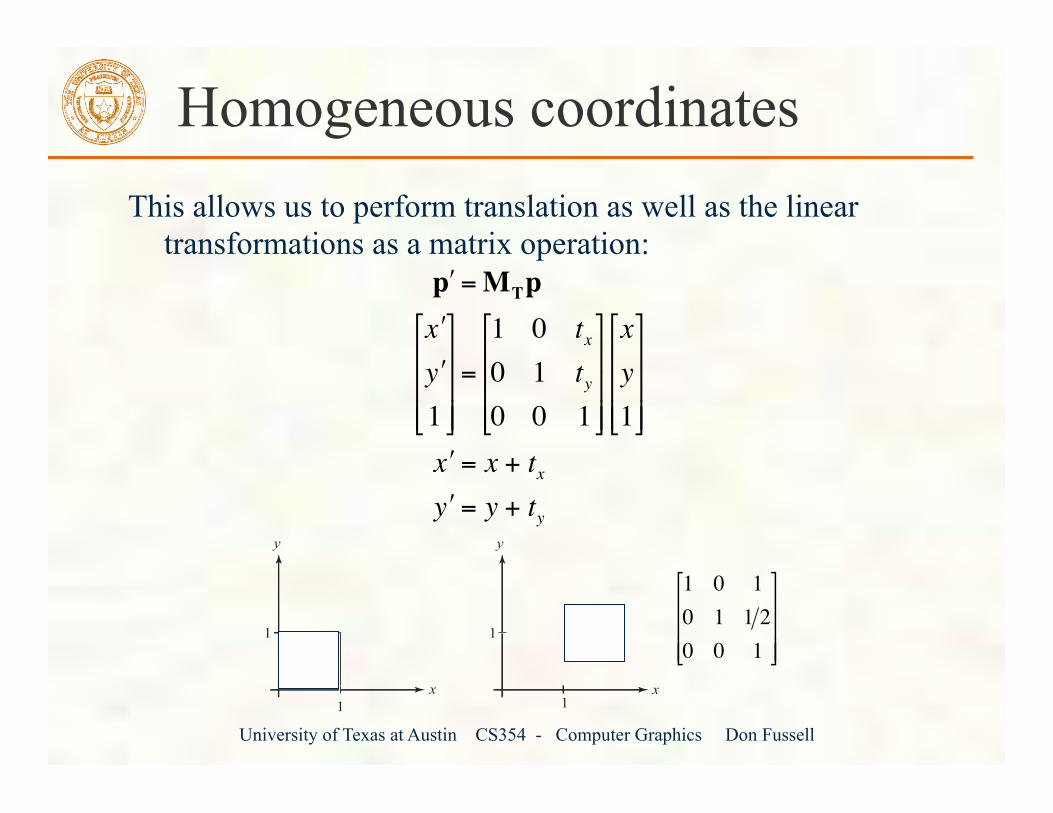
Homogeneous coordinates This allows us to perform translation as well as the linear

transformations as a matrix operation:

€

" p = MTp" x " y 1

#

$

% % %

&

'

( ( (

=

1 0 tx

0 1 ty

0 0 1

#

$

% % %

&

'

( ( (

xy1

#

$

% % %

&

'

( ( (

" x = x + tx

" y = y + ty

1x

y

x

y

1 1

1

€

1 0 10 1 1 20 0 1

"

#

$ $ $

%

&

' ' '


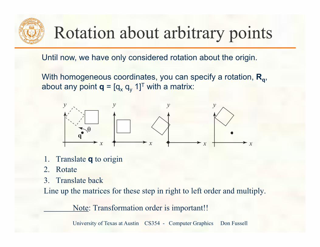
Rotation about arbitrary points

1.  Translate q to origin 2.  Rotate 3.  Translate back Line up the matrices for these step in right to left order and multiply.

Note: Transformation order is important!!

Until now, we have only considered rotation about the origin.

With homogeneous coordinates, you can specify a rotation, Rq, about any point q = [qx qy 1]T with a matrix:

x

y

x

y

x

y

x

y

qθ


Points and vectors From now on, we can represent points as have an additional coordinate of w=1.

Vectors have an additional coordinate of w=0. Thus, a change of origin has no effect on vectors.

Q: What happens if we multiply a matrix by a vector?

These representations reflect some of the rules of affine operations on points and vectors:

One useful combination of affine operations is:

Q: What does this describe?

€

vector + vector →vector ⋅ vector →

point −point →point + vector →

point + point →

€

p(t) = p0 + tv


Barycentric coordinates A set of points can be used to create an affine frame. Consider a triangle ABC and a point p:

We can form a frame with an origin C and the vectors from C to the other vertices:

We can then write P in this coordinate frame

The coordinates (α, β, γ) are called the barycentric coordinates of p relative to A, B, and C.

A

B C

p

€

•

€

p =αu+ βv + t

€

u = A−C v = B−C t = C


Computing barycentric coordinates For the triangle example we can compute the barycentric

coordinates of P:

Cramer’s rule gives the solution:

Computing the determinant of the denominator gives:

€

αA + βB + γC =

Ax Bx Cx

Ay By Cy

1 1 1

%

&

' ' '

(

)

* * *

α

β

γ

%

&

' ' '

(

)

* * *

=

pxpy1

%

&

' ' '

(

)

* * *

€

BxCy − ByCx + AyCx − AxCy + AxBy − AyBx€

α =

px Bx Cx

py By Cy

1 1 1Ax Bx Cx

Ay By Cy

1 1 1

β =

Ax px Cx

Ay py Cy

1 1 1Ax Bx Cx

Ay By Cy

1 1 1

γ =

Ax Bx pxAy By py1 1 1Ax Bx Cx

Ay By Cy

1 1 1


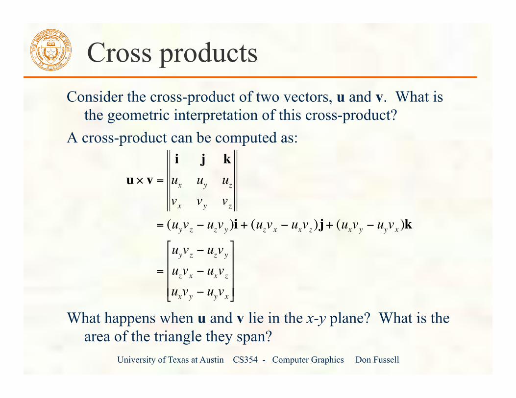
Cross products Consider the cross-product of two vectors, u and v. What is

the geometric interpretation of this cross-product? A cross-product can be computed as:

What happens when u and v lie in the x-y plane? What is the area of the triangle they span?

€

u× v =

i j kux uy uzvx vy vz

= (uyvz − uzvy )i + (uzvx − uxvz)j+ (uxvy − uyvx )k

=

uyvz − uzvyuzvx − uxvzuxvy − uyvx

$

%

& & &

'

(

) ) )


Barycentric coords from area ratios Now, let’s rearrange the equation from two slides ago:

The determinant is then just the z-component of (B-A) × (C-A), which is two times the area of triangle ABC! Thus, we find:

Where SArea(RST) is the signed area of a triangle, which can be computed with cross-products.

€

BxCy − ByCx + AyCx − AxCy + AxBy − AyBx

= (Bx − Ax )(Cy − Ay ) − (By − Ay )(Cx − Ax )

€

α =SArea(pBC)SArea(ABC)

β =SArea(ApC)SArea(ABC)

γ =SArea(ABp)SArea(ABC)


Affine and convex combinations Note that we seem to have added points together, which we said was illegal, but as long as they have coefficients that sum to one, it’s ok.

We call this an affine combination. More generally

is a proper affine combination if:

Note that if the αi ‘s are all positive, the result is more specifically called a convex combination.

Q: Why is it called a convex combination?

11

ni

iα

=

=∑

€

p =α1p1 +…+αnpn


Basic 3-D transformations: scaling

Some of the 3-D transformations are just like the 2-D ones.

For example, scaling:

x x

y

z

y

z

€

" x " y " z 1

#

$

% % % %

&

'

( ( ( (

=

sx 0 0 00 sy 0 00 0 sz 00 0 0 1

#

$

% % % %

&

'

( ( ( (

xyz1

#

$

% % % %

&

'

( ( ( (


Translation in 3D

x x

y

z

y

z

€

" x " y " z 1

#

$

% % % %

&

'

( ( ( (

=

1 0 0 tx

0 1 0 ty

0 0 1 tz

0 0 0 1

#

$

% % % %

&

'

( ( ( (

xyz1

#

$

% % % %

&

'

( ( ( (


Rotation in 3D Rotation now has more possibilities in 3D:

x

z

y

xR

yR

zR

Use right hand rule

€

Rx (θ) =

1 0 0 00 cos(θ) −sin(θ) 00 sin(θ) cos(θ) 00 0 0 1

$

%

& & & &

'

(

) ) ) )

Ry (θ) =

cos(θ) 0 sin(θ) 00 1 0 0

−sin(θ) 0 cos(θ) 00 0 0 1

$

%

& & & &

'

(

) ) ) )

Rz(θ) =

cos(θ) −sin(θ) 0 0sin(θ) cos(θ) 0 00 0 1 00 0 0 1

$

%

& & & &

'

(

) ) ) )


Shearing in 3D

 Shearing is also more complicated. Here is one example:

 We call this a shear with respect to the x-z plane.

x x

y

z

y

z

€

" x " y " z 1

#

$

% % % %

&

'

( ( ( (

=

1 b 0 00 1 0 00 0 1 00 0 0 1

#

$

% % % %

&

'

( ( ( (

xyz1

#

$

% % % %

&

'

( ( ( (


Preservation of affine combinations A transformation F is an affine transformation if it preserves affine

combinations:

where the pi are points, and:

Clearly, the matrix form of F has this property. One special example is a matrix that drops a dimension. For example:

This transformation, known as an orthographic projection, is an affine transformation.

We’ll use this fact later…

11

ni

iα

=

=∑

€

" x " y 1

#

$

% % %

&

'

( ( (

=

1 0 0 00 1 0 00 0 0 1

#

$

% % %

&

'

( ( (

xyz1

#

$

% % % %

&

'

( ( ( (

€

F(α1p1 +…+αnpn ) =α1F(p1 ) +…+αnF(pn )


Properties of affine transformations

 Here are some useful properties of affine transformations:

Lines map to lines Parallel lines remain parallel Midpoints map to midpoints (in fact, ratios are always preserved)

p

q

rp'

q'

r's

t

st

:

:!

€

ratio =pqqr

=st

=" p " q " q " r

Next Lecture   More Math and Transforms


Programming tips  3D graphics, whether OpenGL or Direct3D or any other API, can be frustrating

You write a bunch of code and the result is

Nothing but black window; where did your rendering go??


Things to Try   Set your clear color to something other than black!

It is easy to draw things black accidentally so don’t make black the clear color But black is the initial clear color

  Did you draw something for one frame, but the next frame draws nothing? Are you using depth buffering? Did you forget to clear the depth buffer?

  Remember there are near and far clip planes so clipping in Z, not just X & Y   Have you checked for glGetError?

Call glGetError once per frame while debugging so you can see errors that occur For release code, take out the glGetError calls

  Not sure what state you are in? Use glGetIntegerv or glGetFloatv or other query functions to make sure that OpenGL’s state is what you think it is

  Use glutSwapBuffers to flush your rendering and show to the visible window Likewise glFinish makes sure all pending commands have finished

  Try reading http://www.slideshare.net/Mark_Kilgard/avoiding-19-common-opengl-pitfalls This is well worth the time wasted debugging a problem that could be avoided


Thanks

 Material for these slides provided by Christian Miller


vector and affine math - university of texas at austinfussell/courses/cs354/lectures/...vector...

Documents