vashon-maury island phase 1 groundwater model
TRANSCRIPT

Vashon-Maury Island Phase I Groundwater Model
A part of the Vashon-Maury Island
Water Resource Evaluation
October 2005
Alternate Formats Available 206-296-7380 TTY Relay: 711

King County Department of Natural Resources and Parks
Vashon-Maury Island Phase I Groundwater Model A part of the Vashon-Maury Island Water Resource Evaluation Submitted by: Ken Johnson King County Water and Land Resources Division Department of Natural Resources and Parks
Department of Natural Resources and ParksWater and Land Resources Division201 S Jackson St. Ste 600Seattle, WA 98104(206) 296-6519

King County Department of Natural Resources and Parks - i -
EXECUTIVE SUMMARY King County Department of Natural Resources and Parks (DNRP) has prepared a Phase I model of groundwater flow on Vashon-Maury Island (VMI). This is a part of the VMI Water Resources Evaluation, a multi-year effort which will assess the quantity of water resources available and the threats to its sustainability. This is the first attempt to model groundwater flow over the entire Island. The model uses the USGS MODFLOW-2000 system, a finite difference model, through the Visual MODFLOW pre- and post-processing software. The model employs a steady-state approach (average conditions) with a grid of 41 columns by 67 rows, each 1000 feet on a side. It has 10 layers that model 4 aquifers and 3 aquitards, from ground surface to more than 400 feet below sea level. The stratigraphy was based on a 3-D database of borings and well logs compiled by the UW Pacific Northwest Center for Geologic Mapping Studies (GeoMapNW). Boundary conditions include wells, recharge (natural and septic drainfields), streams, springs, and deep discharge to Puget Sound. The modeling effort indicated uncertainties about some the quantity of well production – agricultural irrigation in particular is not well understood. Calibration was accomplished by successively modifying aquifer/aquitard properties (hydraulic conductivity) and some lesser-defined boundary conditions (streams and springs) to successively improve the fit. For simplicity, the properties for any given unit (aquifer and aquitard) were considered to be uniform across the entire Island, as were the boundary condition parameters for all streams and springs. The measure of fitness for a calibration run was defined by the difference (residual) between observed and model-estimated water levels in 40 target wells, with water levels ranging from sea level to more than 300 feet above sea level. The final calibration fit this data set with a correlation coefficient of 0.87 and a residual mean of 4.5 feet. Sensitivity analyses indicate that the model is most sensitive to hydraulic conductivity in medium deep units (Qpf and QAc), although this sensitivity may be associated with the Puget Sound boundary condition (located in the Qpf layer). Less sensitive were the conductivities in shallower and deeper units and the stream and springs boundary condition parameters. Many features that have been observed previously about the Island’s groundwater can be replicated and compared in the model. Total recharge to the aquifers, after removal of evapotranspiration and direct runoff, is estimated to be 16,694 gallons per minute. The overall water balance in the present model is similar to previous estimates of total flows in the various components, although the estimated amount of discharge to Puget Sound may be larger in the present model than in previous studies: 27% of precipitation compared to 14% estimated in the VMI Groundwater Management Plan (VMI GWAC 1998). Other boundary conditions show smaller flows: wells remove about 2% of the original precipitation and springs release about 1%. Flows to the stream boundary conditions (about 4% of precipitation) agree reasonably well with actual base flow measurements conducted in recent months. The model demonstrates many aspects of groundwater flow on the island. Water level contours are flat in the middle of the Island, and drop off steeply at its edge. Groundwater gradients (and

King County Department of Natural Resources and Parks - ii -
thus flows) are downward throughout the island, although somewhat less along the coastline, where deep groundwater must flow up towards Puget Sound discharge locations. An example of application of the model is given for a scenario where all population-related water use is increased by 10%. This illustrative example yields noticeable drawdown in the vicinity of some Group A water system wells, though generally very small numerically, and it also shows slightly higher shallow groundwater levels in many other areas of the Island, where the increased septic system returns occur. The report concludes with recommendations of improvements to be considered in subsequent investigation and modeling efforts on VMI.

King County Department of Natural Resources and Parks - iii -
TABLE OF CONTENTS EXECUTIVE SUMMARY ............................................................................................................. I TABLE OF CONTENTS.............................................................................................................. III LIST OF TABLES........................................................................................................................ IV LIST OF FIGURES ...................................................................................................................... IV 1.0 INTRODUCTION ................................................................................................................... 1
1.1 Study Area ........................................................................................................................... 1 1.2 Purpose of Model................................................................................................................. 1 1.3 Modeling Overview ............................................................................................................. 2
2.0 MODEL DESCRIPTION ........................................................................................................ 4 2.1 Model Grid........................................................................................................................... 4 2.2 Model Layers or Hydrostratigraphy .................................................................................... 4 2.3 Aquifer Properties................................................................................................................ 9 2.4 Boundary Conditions (BC) ................................................................................................ 12
2.4.1 Wells (Pumping Well Boundary Conditions) ............................................................. 14 2.4.2 Streams (River Boundary Conditions)........................................................................ 19 2.4.3 Recharge (BC) ............................................................................................................ 23 2.4.4 Springs (Drain Boundary Conditions) ........................................................................ 25 2.4.5 Discharge to Puget Sound (Fixed Head Boundary Conditions) ................................. 27
3.0 PROCESS OF MODELING.................................................................................................. 28 4.0 IMULATION RESULTS....................................................................................................... 34
4.1 Component Water Balance ................................................................................................ 34 4.2 Streams and Springs........................................................................................................... 37 4.3 Water Level Contours........................................................................................................ 42 4.4 Sensitivity Analyses........................................................................................................... 44 4.5 Gain in Understanding ....................................................................................................... 46 4.6 Predictive Runs .................................................................................................................. 47
5.0 RECOMMENDATIONS FOR SUBSEQUENT WORK...................................................... 51 5.1 Hydrostratigraphy .............................................................................................................. 51 5.2 Aquifer Properties.............................................................................................................. 51 5.3 Grid Spacing ...................................................................................................................... 52 5.4 Boundary Conditions ......................................................................................................... 53 5.5 Transient Flow Conditions................................................................................................. 53 5.6 Calibration / Validation Data............................................................................................. 54
6.0 REFERENCES ...................................................................................................................... 55

King County Department of Natural Resources and Parks - iv -
LIST OF TABLES Table 1-1 Model Stratigraphic Layers............................................................................................9
Table 1-2 Aquifer Parameter Data ...............................................................................................11
Table 1-3 Total Well Production Rates........................................................................................19
Table 1-4 Total Model Recharge Components ............................................................................25
Table 2-1. Calibrated Hydraulic Conductivities............................................................................32
Table 4-1 Inflows and Outflows in Model ...................................................................................35
Table 4-2 Comparison of Model Water Balance to Previous Studies..........................................37
Table 4-3 Results of Sensitivity Analyses....................................................................................44
LIST OF FIGURES Figure 1-1 Flowchart of Steps to Build a Groundwater Model. (NGWA 2004)............................3
Figure 2-1 Model Grid.....................................................................................................................5
Figure 2-2a, b East-West Cross Section near Burton (see Figure 2-1)..........................................8
Figure 2-3 Extent of Model (Schematic) .......................................................................................13
Figure 2-4 PWS Service Areas and Estimated Individual Well Locations ...................................15
Figure 2-5 Total Well Production per Model Cell.........................................................................20
Figure 2-6 Stream Boundary Conditions and Gaging Locations...................................................22
Figure 2-7 Average Precipitation Used in Model..........................................................................24
Figure 2-8 Recharge Boundary Condition Total Flows ................................................................26
Figure 3-1 Target Water Level Well Locations.............................................................................30
Figure 3-2 Calibration Results: Model (calculated) vs. Target (observed) ...................................31
Figure 4-1 Water Balance Details (flows in gpm).........................................................................36
Figure 4-2 River flows: Gauged Data vs. Model Totals................................................................38
Figure 4-3 River Boundary Condition Locations and Flows.........................................................40
King County Department of Natural Resources and Parks - v -
Figure 4-4 Spring Boundary Condition Locations and Flows.......................................................41
Figure 4-5a, b Water Level Contour Output.................................................................................42
Figure 4-6 Cross-Section Graphical Output ..................................................................................43
Figure 4-7 Model-Estimated Head Difference Between Qva and QAc Aquifers .........................48
Figure 4-8 Drawdown for Increased Pumpage (Layer 4, plan view) ............................................49
Figure 4-9 Drawdown for Increased Pumpage (Model Row 43) ..................................................50

King County Department of Natural Resources and Parks - 1 -
1.0 INTRODUCTION
The Water Resource Evaluation Project is intended to cover monitoring, modeling, and data management activities within Vashon-Maury Island (VMI) for seven years (2004-2010). As part of this work, a groundwater model was created to help address the water balance concerns on VMI. Understanding the water budget for Vashon-Maury Island and how it changes in response to human activities and climate changes is important in determining the amount of drinking water that can be used on a sustained basis.
This report provides an overview of the modeling and preliminary findings. The structure of the report is as follows: Section 1.0 - introduction and overview; Section 2.0 – model description; Section 3.0 – process of modeling; Section 4.0 – simulation results; and Section 5.0 – recommendations for subsequent work.
1.1 STUDY AREA
Vashon-Maury Island lies in the Puget Lowland encompassing about 36 square miles. The Island is composed of glacial derived sediments deposited during several glacial episodes. The predominant geology on Vashon-Maury Island is glacial till. This geology covers approximately 68% of the Island and helps define the topography. The remaining 32% of the Island is made of glacial outwash and alluvial deposits. All drinking water sources on the island (springs, surface water, and groundwater) are supplied by precipitation on the Island. Vashon-Maury Island was designated a Sole Source Aquifer by the United States Environmental Protection Agency in June 1994. Water quality on Vashon-Maury Island is generally good.
Groundwater is the portion of precipitation that soaks into the ground and gets stored in underground geological water systems called aquifers. Every groundwater system is unique and dependent upon external factors such as the rate of precipitation, the interaction of groundwater with the streams and other surface water bodies, the rate of evapotranspiration, and in the case of an island, interactions with the surrounding open water.
1.2 PURPOSE OF MODEL King County has developed an initial (Phase I), three-dimensional model of steady-state groundwater flow in the aquifers underlying Vashon-Maury Island, with the main purpose of summarizing the state of knowledge of groundwater on the Island. Phase I represents an initial effort to model the Island’s groundwater hydrology. Other Phases will be based on this work. The main overall purpose of the model is really to test our understanding of the Island aquifers, and to improve that understanding. Water Balance: The model can be used to estimate the overall water balance for the Island. A water balance is an accounting of the quantity of water entering and leaving the groundwater systems (aquifers) on the island. It estimates how much water comes from various sources, such

King County Department of Natural Resources and Parks - 2 -
as precipitation, on-site sewage (or septic) systems, and streams. Similarly, the model estimates how much water goes from the aquifer to the various discharge mechanisms, including wells, springs, streams, and deep (subsurface) discharge to Puget Sound. Several attempts have been made in the past to estimate an overall water balance for the Island. Two main differences regarding the water balance developed in this modeling effort, as compared to the previous reports, is that:
• components are spatially-distributed at appropriate locations across the Island. • the depths of the inflows and outflows are estimated and accounted for.
In previous estimates, water pumped from a deep well on Maury Island may be balanced against upland stream flows in Shinglemill Creek on Vashon Island despite their very different locations and depths. Instead this model requires that such spatial differences be stated explicitly, and their consequences be considered in the analysis.
1.3 MODELING OVERVIEW
The modeling process has numerous steps (Figure 1-1) that are outlined here, accomplished in the modeling process, and will be expanded upon in Section 3.0. The initial process of modeling after defining purpose and scope is to create a conceptual model. This step is the most important because this step helps guide the scale, geology/hydrogeology and the type of model necessary to address the purpose of the project. The conceptual model guided the model development and thus is discussed in Section 2.0. The next step is to set up the model with layers, a grid, boundary conditions, and aquifer properties. All of these items are explained in greater detail in Section 2.0. After model setup is complete, calibration (the adjustment of the computer model to better reflect measurements) is necessary to obtain useful information. Details of the VMI calibration can be found in Section 3.0 Another step often done is validation (comparing model output to an independent set of observations); unfortunately, this validation step was not possible for the VMI model due to the lack of an independent time period with sufficient data to perform this step. Through the iterative process, the model simulations become more representative of natural conditions. Model Limitations: A model is a generalized representation of the natural system. It cannot be considered a perfect representation of the system hydrology. This means limitations are created in the process. Generalization in the hydrogeology is typically the greatest limitation due to uncertainty or data gaps in this aspect. Another limitation of a groundwater model is due to the coarse scale (spatial discretization) of the model. Being a coarse representation of the natural system infers that certain features will be different in the model than in reality. An example is the need to replace a number of wells within a wide area with one representative well in the cell, keeping the total pumpage the same. The cells are 1,000 feet on each side, thus slightly smaller than a quarter-quarter Section (1,320’ on each side), and there can be several residences (i.e., wells) within this area.

King County Department of Natural Resources and Parks - 3 -
Figure 1-1 Flowchart of Steps to Build a Groundwater Model. (NGWA 2004).
A third, and most significant, limitation on the model is that many of the flow components have not been measured. Some of the model inputs are directly derived from well-known data sources and are simply imposed on the model, such as how many people (total) reside on the Island, which determines approximately how much water they use, and how much water is produced by the largest (Group A) water purveyors. However, it is not exactly known how much is pumped by the smaller (Group B) systems or how much water is pumped from individual wells; and finally how much water is used for irrigation.
King County Department of Natural Resources and Parks - 4 -
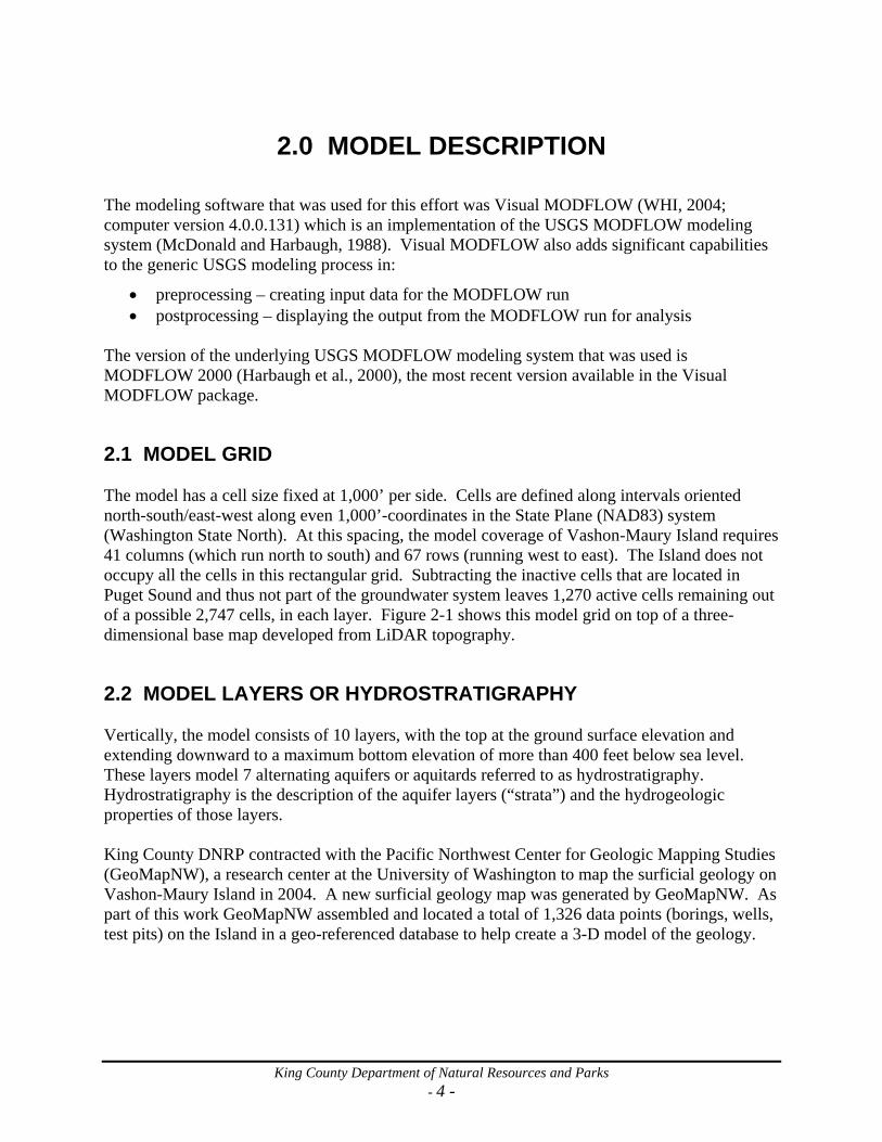
2.0 MODEL DESCRIPTION The modeling software that was used for this effort was Visual MODFLOW (WHI, 2004; computer version 4.0.0.131) which is an implementation of the USGS MODFLOW modeling system (McDonald and Harbaugh, 1988). Visual MODFLOW also adds significant capabilities to the generic USGS modeling process in:
• preprocessing – creating input data for the MODFLOW run • postprocessing – displaying the output from the MODFLOW run for analysis
The version of the underlying USGS MODFLOW modeling system that was used is MODFLOW 2000 (Harbaugh et al., 2000), the most recent version available in the Visual MODFLOW package.
2.1 MODEL GRID The model has a cell size fixed at 1,000’ per side. Cells are defined along intervals oriented north-south/east-west along even 1,000’-coordinates in the State Plane (NAD83) system (Washington State North). At this spacing, the model coverage of Vashon-Maury Island requires 41 columns (which run north to south) and 67 rows (running west to east). The Island does not occupy all the cells in this rectangular grid. Subtracting the inactive cells that are located in Puget Sound and thus not part of the groundwater system leaves 1,270 active cells remaining out of a possible 2,747 cells, in each layer. Figure 2-1 shows this model grid on top of a three-dimensional base map developed from LiDAR topography.
2.2 MODEL LAYERS OR HYDROSTRATIGRAPHY Vertically, the model consists of 10 layers, with the top at the ground surface elevation and extending downward to a maximum bottom elevation of more than 400 feet below sea level. These layers model 7 alternating aquifers or aquitards referred to as hydrostratigraphy. Hydrostratigraphy is the description of the aquifer layers (“strata”) and the hydrogeologic properties of those layers. King County DNRP contracted with the Pacific Northwest Center for Geologic Mapping Studies (GeoMapNW), a research center at the University of Washington to map the surficial geology on Vashon-Maury Island in 2004. A new surficial geology map was generated by GeoMapNW. As part of this work GeoMapNW assembled and located a total of 1,326 data points (borings, wells, test pits) on the Island in a geo-referenced database to help create a 3-D model of the geology.

King County Department of Natural Resources and Parks - 5 -
Figure 2-1 Model Grid
Note: Image shows model grid draped on a 3-D LiDAR basemap.
Cross Section along model row 43 (Figure 2-2a, b)

King County Department of Natural Resources and Parks - 6 -
Each of the data points describes the subsurface layers (in the vicinity of the points) over the Island. The data as found in these logs was entered and compiled into a database that was linked to the point locations. Each of the 6,564 data points (approximately 5 per each boring) was entered into the database with a summary of its main soil constituents (clay, silt, sand, gravel, organics, debris) as well as according to standardized classification. The reported depth of each layer was converted to elevation based on surveyed elevations across the Island obtained via Light Detection and Ranging (LiDAR). The individual layer description data from GeoMapNW were further categorized into a smaller number (three) of basic hydrogeologic material types:
• Aquifers – clean (low silt or clay) sands and / or gravels, or described as “water bearing” or “outwash”
• Tills – silt and sand (or gravel) mixtures, or described as “till” or “hardpan” in the well logs
• Clays – materials that include clay as a significant component, or are mostly silt Till and clay layers were then grouped together as aquitards (layers that conduct water poorly) for the purposes of delineating the aquifer and aquitards across the Island. GeoMapNW developed an automatic analysis tool (Borehole Data Display) that puts all these stratigraphic data along a specific alignment to produce a cross-section. An example of a cross section across Vashon and Maury Island, which was developed using this tool, is shown in Figure 1-2b. GeoMapNW also prepared an auxiliary database that includes water level information. These water levels could be provided on cross sections using another analysis tool, Downhole Data Display. The Phase I model incorporates many of the layers described in these logs, beginning with the ground surface. The LiDAR data was used to describe the ground surface; this provides the top of the grid (top of Layer 1 - see Figure 1-1). From this elevation downward, at every active cell in the model, a total of 10 layers were input to the model. The first subsurface stratigraphic layer to be estimated was the base of the Vashon Advance Outwash aquifer, Qva, which was used in the model as the base of model layer 4. GeoMapNW had already developed a contour map of this surface in support of the susceptibility mapping for King County’s Critical Aquifer Recharge Area. This contour map was obtained from GeoMapNW in a GIS form, and the contour lines were interpolated over the entire Island using Surfer (v. 8.05, Golden Software, 2002) and specifically the kriging method. Elevations for the other layers were then developed, working from the base of the Qva, by considering each of the aquifer layers in the GeoMapNW database in each boring in a given cell. The hydrostratigraphy was very irregular among the different borings, with various pieces of aquifer and aquitard showing up in any interval being examined (see examples in cross-section in Figure 2-2b). These varied pieces of the overall picture had to be melded into a unified representation for use in the model. Each next interface (top / bottom of the next layer down) elevation was derived from interpolation of three separate measures: the elevation of the bottom of the pieces (sublayers) of aquifer/aquitard in the interval, the sublayer thicknesses (subtracted from the layer above), and the elevation of the top of the deeper sublayer. For example, the base
King County Department of Natural Resources and Parks - 7 -
of the Qpf, the (aquitard) unit immediately below the Qva, would be estimated by the following components, each of which may be found at different depths or thicknesses in several borings in the model cell: Zbase (Qpf) = average of:
Zbase of 1st aquitard sublayer below Qva Ztop of 1st aquifer sublayer below Qva Zbase (Qva) minus the thickness of 1st aquitard sublayer below Qva
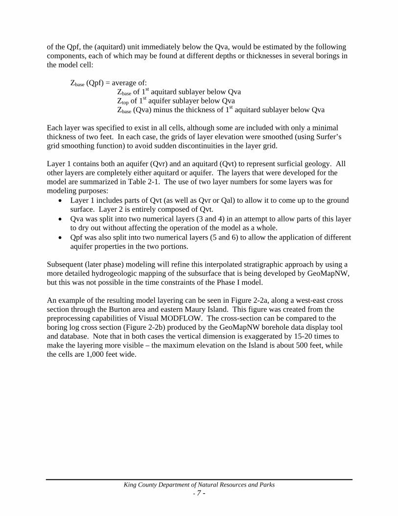
Each layer was specified to exist in all cells, although some are included with only a minimal thickness of two feet. In each case, the grids of layer elevation were smoothed (using Surfer’s grid smoothing function) to avoid sudden discontinuities in the layer grid. Layer 1 contains both an aquifer (Qvr) and an aquitard (Qvt) to represent surficial geology. All other layers are completely either aquitard or aquifer. The layers that were developed for the model are summarized in Table 2-1. The use of two layer numbers for some layers was for modeling purposes:
• Layer 1 includes parts of Qvt (as well as Qvr or Qal) to allow it to come up to the ground surface. Layer 2 is entirely composed of Qvt.
• Qva was split into two numerical layers (3 and 4) in an attempt to allow parts of this layer to dry out without affecting the operation of the model as a whole.
• Qpf was also split into two numerical layers (5 and 6) to allow the application of different aquifer properties in the two portions.
Subsequent (later phase) modeling will refine this interpolated stratigraphic approach by using a more detailed hydrogeologic mapping of the subsurface that is being developed by GeoMapNW, but this was not possible in the time constraints of the Phase I model. An example of the resulting model layering can be seen in Figure 2-2a, along a west-east cross section through the Burton area and eastern Maury Island. This figure was created from the preprocessing capabilities of Visual MODFLOW. The cross-section can be compared to the boring log cross section (Figure 2-2b) produced by the GeoMapNW borehole data display tool and database. Note that in both cases the vertical dimension is exaggerated by 15-20 times to make the layering more visible – the maximum elevation on the Island is about 500 feet, while the cells are 1,000 feet wide.

King County Department of Natural Resources and Parks - 8 -
2-2a
2-2b
Ke r
mit
Ge o
ring
John
Far
rell
R R
oar k
Chr
is K
e y
Ral
p h W
il lia
ms
B-1
Don
a ld
E Tu
rne r
4 1-V
eltm
an
Chr
is C
erba
Joe
Van o
sGre
g ory
J M
art in
Tom
For
me l
la
Ros
s M
ayb e
rry
Ba r
ry G
e lba
rt
Dan
May
e r
L in
Ho l
ley
& M
i ke
Tem
plem
an
Chr
is O
lse n
H K
n igh
t
B-2
B-1
MW
-B
Jim
Sco
t t
T om
Le h
ma n
9 5-N
e lso
n
Mi k
e R
a nd
Dal
e R
adel
Ed w
in E
b rig
ht
MW
-1
MW
-2
Geo
rge
Edw
ard s
8 4-S
chm
idt
Clif
f Lin
dgre
n
4 4-P
ars o
nsJo
e C
u nni
ngh a
m
Nan
cy S
ton i
ngto
n
Be r
ry P
i tt
W N
a rva
rso n
9 3-N
e lso
nD
oyle
Mi la
n
John
Fol
ey
Daw
son
(Mis
ty Is
l es0
B-3
Ke r
nel l
(Mis
ty Is
les)
B-4
Ka r
eem
Ab d
ul
R O
lsen
Ma t
t Pax
ton
Art
Ho d
gki n
s
Cel
i a S
org e
T om
Stu
a rt (
DSA
)
Ed s
al H
arris
Bo b
Tu c
ker
5 0-M
il ler
Jan
Smith
J im
Sco
t t
Ma r
gare
t Sm
i th
OS
A
Hen
ry S
auer
Be r
ry P
i t t
Dar
rel l
De v
os
Ma r
k D
egro
ot
Don
Ra y
mon
d
Mi k
e Fl
ynn
MW
-3
KIR
O
P C
h ris
F ran
k Ze
llerh
off
Ste
ve S
telle
rK
e n W
aits
-400
-350
-300
-250
-200
-150
-100
-50
0
50
100
150
200
250
300
350
400
0
2000
4000
6000
8000
1000
0
1200
0
1400
0
1600
0
1800
0
2000
0
2200
0
2400
0
2600
0
2800
0
3000
0
Figure 2-2a, b East-West Cross Section near Burton (see Figure 2-1).
Notes: 2-2a: in model (model row 43): solid color cells under Quartermaster Harbor are inactive, the other
colors represent the layers with their varying hydraulic conductivity values; 2-2b: in UW database cross-section, colors represent soil characteristics:
Geologic units are: Qvr = Vashon Recessional Outwash aquifer; Qvt = Vashon Till aquitard; Qva = Vashon Advance Outwash aquifer; Qpf = PreFraser Interglacial (aquitard); QAc = upper deep aquifer; QBf = deep aquitard; QBc = lower deep aquifer; QC = deeper aquifer / aquitard.
Some well logs (especially on eastern Maury Island) are projected onto cross section from higher ground to south and thus do not align with plotted ground surface.
Qvr Qvt
Qva Qpf
QAc QC
Blue = sandy Green = clayey Yellow = gravelly Gray = silty
Inactive cells
Quartermaster Harbor (north of Burton peninsula)
Maury Island Fisher CreekChristensen Creek
QBf QBc
King County Department of Natural Resources and Parks - 9 -
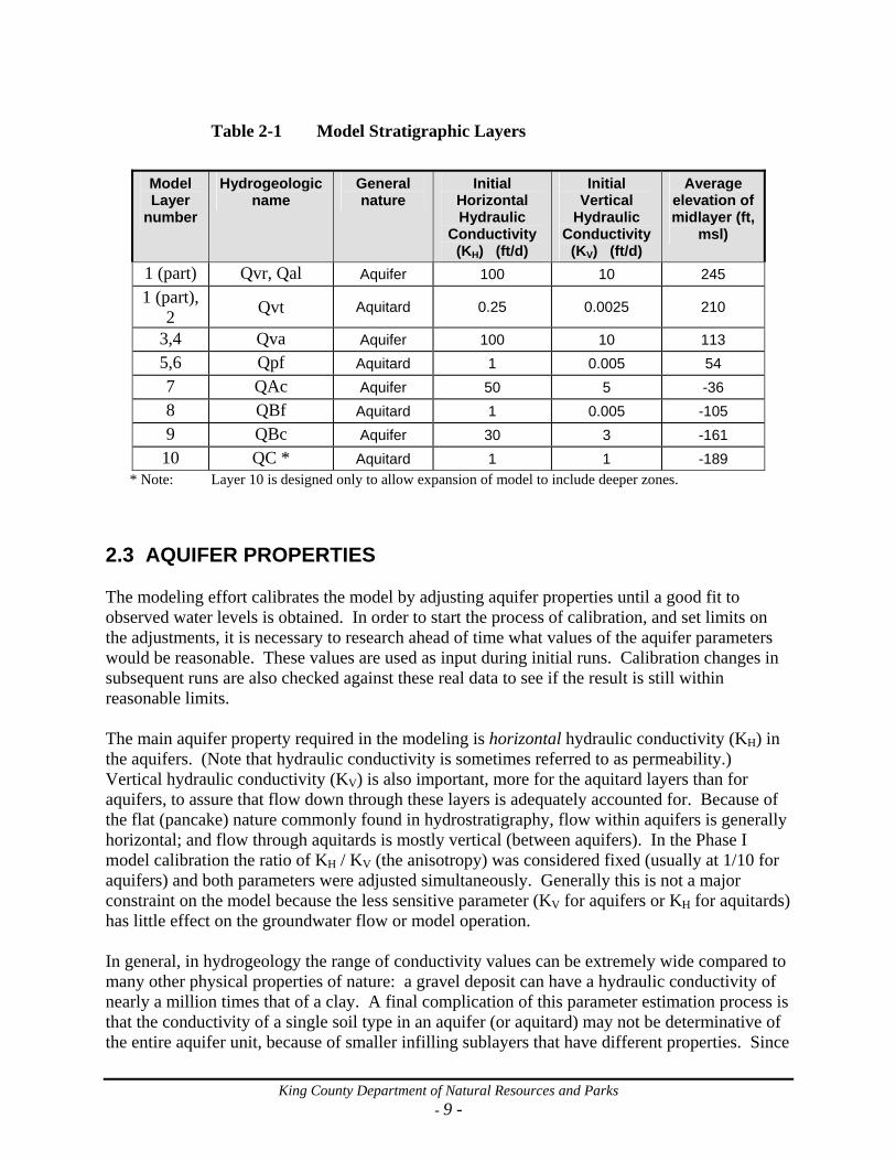
Table 2-1 Model Stratigraphic Layers
Model Layer
number
Hydrogeologic name
General nature
Initial Horizontal Hydraulic
Conductivity (KH) (ft/d)
Initial Vertical
Hydraulic Conductivity
(KV) (ft/d)
Average elevation of midlayer (ft,
msl)
1 (part) Qvr, Qal Aquifer 100 10 245 1 (part),
2 Qvt Aquitard 0.25 0.0025 210
3,4 Qva Aquifer 100 10 113 5,6 Qpf Aquitard 1 0.005 54 7 QAc Aquifer 50 5 -36 8 QBf Aquitard 1 0.005 -105 9 QBc Aquifer 30 3 -161 10 QC * Aquitard 1 1 -189
* Note: Layer 10 is designed only to allow expansion of model to include deeper zones.
2.3 AQUIFER PROPERTIES The modeling effort calibrates the model by adjusting aquifer properties until a good fit to observed water levels is obtained. In order to start the process of calibration, and set limits on the adjustments, it is necessary to research ahead of time what values of the aquifer parameters would be reasonable. These values are used as input during initial runs. Calibration changes in subsequent runs are also checked against these real data to see if the result is still within reasonable limits. The main aquifer property required in the modeling is horizontal hydraulic conductivity (KH) in the aquifers. (Note that hydraulic conductivity is sometimes referred to as permeability.) Vertical hydraulic conductivity (KV) is also important, more for the aquitard layers than for aquifers, to assure that flow down through these layers is adequately accounted for. Because of the flat (pancake) nature commonly found in hydrostratigraphy, flow within aquifers is generally horizontal; and flow through aquitards is mostly vertical (between aquifers). In the Phase I model calibration the ratio of KH / KV (the anisotropy) was considered fixed (usually at 1/10 for aquifers) and both parameters were adjusted simultaneously. Generally this is not a major constraint on the model because the less sensitive parameter (KV for aquifers or KH for aquitards) has little effect on the groundwater flow or model operation. In general, in hydrogeology the range of conductivity values can be extremely wide compared to many other physical properties of nature: a gravel deposit can have a hydraulic conductivity of nearly a million times that of a clay. A final complication of this parameter estimation process is that the conductivity of a single soil type in an aquifer (or aquitard) may not be determinative of the entire aquifer unit, because of smaller infilling sublayers that have different properties. Since

King County Department of Natural Resources and Parks - 10 -
the model layer thickness is based on the unit’s top and bottom depths, the overall hydraulic conductivity must (mathematically) include the effect of the subunits. This is another example of the simplification process inherent in modeling. Another aquifer property that is frequently used in groundwater modeling is porosity, but this will not be discussed in this report as it is an issue only for transient models (rather than the steady state model here) or for contaminant transport purposes, and will be included in future models as needed. Hydraulic conductivity may be directly estimated from a variety of tests. When a large water supply well is installed the driller or consultant usually conducts a pumping test to determine drawdown (the drop of groundwater level during pumping). This test consists of pumping the well at a relatively high and constant flow rate continuously for a long period (the industry standard is 1-3 days). While the well is pumping, water levels are observed in the well and in nearby wells to observe the effect of the pumping. The drawdown plots (drawdown vs. time, or vs. distance from the pumped well) show characteristics that allow the hydraulic conductivity to be calculated directly. The pumping test as described here is the gold standard for conductivity estimation, as it observes the parameter over a relatively large spatial extent and time frame. A similar but less accurate method for hydraulic conductivity is a pumping test usually conducted by drillers in smaller water supply wells (e.g., domestic wells). In this test a single drawdown water level is measured only in the pumped well itself and for a shorter period of time. The short test can give adequate information for the purposes of well installation and is frequently reported on the driller’s log. The drawdown vs. pumping rate (specific capacity) value reported from this testing can be used to estimate hydraulic conductivity using the method of Cox and Kahle (1999). However, it is representative of only the immediate vicinity of the well screen (which was selected for its likely productivity) and thus may not be applicable to a larger scale. The above two measures of hydraulic properties were used for the present model. Hydraulic conductivity is occasionally estimated on the basis of the size of the particles (“grain size distribution”) in the aquifer, or by “professional judgment”, but such values should be used with extreme caution because they may be inaccurate by orders of magnitude and so were not used for this model. Research for aquifer properties in the present model included documents obtained from the major purveyors (Group A systems) on the Island conducted for a project for the state Health Dept in the year 2000 to locate all the Group A wells in King County precisely using GPS. Another major source of data was the compilation of hydrostratigraphic information (and documents) by GeoMapNW. The state Dept of Ecology was also consulted, for any well information in their files (under the general area designation WRIA 15) and in their compilation of water well logs (now available on-line at http://apps.ecy.wa.gov/welllog/). It was found that there are remarkably few estimates of aquifer properties for the aquifers on Vashon-Maury Island. A summary of the data found is presented in Table 2-2. Additional unanalyzed pumping test data were not used in this model.

King County Department of Natural Resources and Parks - 11 -
Table 3. Aquifer Parameter Data
Source Well / locale Hydrogeologist / citation
Aquifer (approx.)
KH = Horizontal Hydraulic
conductivity (ft/d) Values directly measured on Vashon-Maury Island
KCWD #19 Morgan Hill AGI (1997a) Qva 8* Heights Water Well #3 Rongey (1992) Qva 33
KCWD #19 Gerrior Test Well AGI (1997b) QAc 41* (near well) 12* (at distance)
KCWD #19 Well #2 Carr (1990) QBc 23* Maury Mutual Well #1 Carr (1992) QBc 51*
King Co DNRP, Solid Waste Division
7 Monitoring Wells on landfill site (13 slug
tests)
Berryman & Henigar (2004)
Qva 6 (median) 0.6 – 6.8
Ecology well logs 693 well log tests (using specific capacity
method in Cox & Kahle, 1999)
Drillers’ pump & bailer tests, on Ecology well
logs
Various (not different-
iated)
41 (median) (25%-75% = 12 –
170 ft/d)
Other sources Maury Island Gravel Mine
Hydrogeologic Assessment
Calibrated groundwater flow model of Maury
Island
Pacific Groundwater Group (2000)
Qva Qpf
2.8 – 60 0.03 - 3
Southwest King Co USGS study
General data summary Woodward et al. (1995)
Qva QAc QBc
83 51 51
Bangor Submarine Base Calibrated groundwater flow model (mean
values)
Van Heeswijk & Smith (2002)
Qva QAc QBc
5.3 6.6 4.2
* Calculated from published transmissivity (T), equal to the horizontal hydraulic conductivity of a layer times the thickness of the layer, and the reported screen length Also included in Table 1-2 are data from three other studies in Central Puget Sound glacial units. The study by Pacific Groundwater Group (2000) for the Maury Island Mine indicates representative aquifer parameter values that resulted from the calibration of the groundwater flow model in this area. Two USGS studies (Woodward et al., 1995, and Kahle, 1998) compile or analyze data for areas some distance away from Vashon-Maury Island, both to the east (mainland Southwest King County) and west (Bangor Submarine Base in western Kitsap County). The Southwest King County data are median values of hydraulic conductivity based on pumping tests (or just specific capacity) for wells judged to be in the designated aquifers. Like the specific capacity data taken from VMI wells (row marked “Ecology well logs”) these data are very limited by the local nature of the measurements, the wide range of the aquifer properties as measured (the 25% and 75% quartiles are very different – the high values are 6 times higher than the low ones), and a lack of control for the drillers’ procedures.

King County Department of Natural Resources and Parks - 12 -
The Bangor data are from a calibrated groundwater flow model, so are possibly very applicable to the present work. Other USGS groundwater flow models exist for parts of the Duwamish River valley, Thurston County, Island County, Clallam County, and for a generic Puget Sound condition, but these were not included they were deemed less applicable. The initial estimates of the aquifer properties (hydraulic conductivities) used for the various hydrostratigraphic layers in the present model are shown in Table 2-1. These initial estimates were then adjusted through the calibration process (see Section 2.0).
2.4 BOUNDARY CONDITIONS (BC) The groundwater flow model includes only those physical processes that occur in the saturated soils (Figure 2-3); for example, surface runoff and evapotranspiration are not included. The equations that constitute the main computational system deal with Darcy’s Law for flow only inside the saturated porous media (shown in the figure by a red boundary). Thus, for example, the complicated flow through the unsaturated (vadose) zone above the water table is not computed, but rather the recharge is estimated externally from the modeling effort and simply imposed on the model by flows into the aquifer at the water table (highest active model cells at every location on the Island). The influences of all the other components of the hydrologic cycle are connected at the boundaries of the model extent (the saturated soils) via boundary conditions. Boundary conditions are a mathematical construct that embed the mathematical problem within the real world and allow changes in the model to be accomplished by flows of water in or out of the model.

King County Department of Natural Resources and Parks - 13 -
Figure 2-3 Extent of Model (Schematic)
(Adapted from Turney et al., 1995) The present model includes five kinds of boundary conditions, which are described in the subsequent sections (and are illustrated in Figure 2-3 as blue circles):
• Wells (Section 2.4.1) – cause flow out of the model (into a well) at a specified flow rate. • Streams (2.4.2) – cause flow into or out of the model (from or into a stream) according to
the specified water level in the stream compared to the model groundwater level and the permeability of the stream bed.
• Recharge (2.4.3) – causes inflow to the uppermost active cell at a location as specified by recharge estimates previously reported by DNRP. Lakes are not included in the original recharge estimates, so were added to this boundary condition. Septic system drain field discharges are also introduced to the model via the recharge boundary condition.
• Springs (2.4.4) – cause outflow (but not inflow) from the model according to the spring level (compared to groundwater levels in the model) and the permeability of the interface.

King County Department of Natural Resources and Parks - 14 -
If the groundwater level goes below the level of the springs, the springs go dry and no discharge occurs.
• Discharge to Puget Sound (2.4.5) – allows flow to deep cells along the edge of the model that are assumed to be in direct contact with the bottom of the Sound.
The boundary conditions also bring into the model development a question of time frame. While the hydrostratigraphy (Section 1.4) and the properties of the aquifers (Section 1.5) are generally static (do not change with time), boundary conditions may change over time. Recharge varies with rainfall and climatic variations; runoff, springs flows, and discharges to the Sound vary with precipitation and aquifer levels, and pumpage from wells changes with development, both population increases and changes in land use. For the purposes of the modeling, a uniform time period of calendar year 2001 (as possible) was applied for the driving pumpage boundary conditions while the calibration water level targets were chosen slightly later: June 2001 through May 2002, to account for the delay between cause and effect. These dates allowed much of the available volunteer water level data to be included, and occurred just before a period of drought that continued for some time after. Precipitation recharge was based on estimates that had already been developed for the VMI Water Resource Evaluation, and are based on normal (30-year average) precipitation quantities and spatial variations, so are slightly different from the time basis of the other boundary conditions.
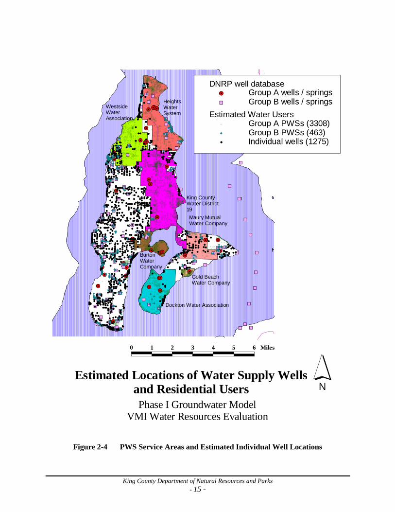
2.4.1 Wells (Pumping Well Boundary Conditions) Well boundary conditions are probably the most easily understood of the boundary conditions because most people are familiar with wells. And the mathematics are simple – just a known flow out of the model from the aquifer at the depth of the well screen. However, despite the intrinsic simplicity of the concept, the actual data to impose the well boundary condition turned out to be somewhat complicated to obtain in its entirety. Different methods had to be used for different categories of wells: the large public water systems (Section 2.4.1.1) have much data available – these are mainly located in the northeastern part of Vashon Island as well as across much of Maury Island (see Figure 2-4). Smaller systems (Section 2.4.1.2) have some data available, and individual wells (Section 2.4.1.3) are practically unknown. These smaller wells are located predominantly in the southwestern portion of Vashon. Agricultural wells (Section 2.4.1.4) have even less information about pumpage or location, so more analysis had to be performed. By depth, it was found that the sources of well pumpage is fairly evenly divided among from the Qva aquifer (or in aquitards just above or below it, a total of 32%), from the upper deep aquifer (QAc, 31%), and from the deeper QBc aquifer (27%). The shallow Qvr aquifer provides only about 10% of the pumpage.
King County Department of Natural Resources and Parks - 15 -
0 1 2 3 4 5 6 Miles
NEstimated Locations of Water Supply Wells
and Residential UsersPhase I Groundwater Model
VMI Water Resources Evaluation
%U
%U%U
%U
%U%U%U%U
%U%U%U%U
%U
%U%U%U
%U%U%U %U%U
%U%U
%U%U%U %U %U%U%U %U%U %U
%U
%U%U %U%U%U%U
%U%U
%U
%U%U%U
%U %U%U
%U%U
%U %U %U%U %U%U%U %U%U%U%U
%U %U%U%U %U %U%U%U%U%U %U%U %U%U %U%U%U %U%U%U %U%U
%U %U%U%U%U %U
%U %U%U %U
%U
%U%U
%U
%U%U%U%U
%U%U %U
%U%U%U%U%U %U
%U%U
%U %U%U%U%U%U%U %U
%U
%U%U%U
%U%U%U%U%U%U
%U
%U
%U%U
%U
%U
%U
%U%U%U
%U %U%U%U%U %U%U
%U
%U%U
%U%U
%U
%U
%U%U
%U
%U
%U
%U%U
%U%U%U%U
#Y
#Y#Y#Y#Y #Y#Y#Y
#Y#Y#Y#Y#Y#Y
#Y
#Y
#Y
#Y#Y
#Y
#Y
#Y
#Y#Y#Y
#Y #Y#Y#Y#Y#Y#Y
#Y
#Y#Y
#Y
#Y
#Y#Y
#Y
#Y
#Y#Y
#Y
#Y
#Y
#Y#Y
#Y#Y#Y#Y#Y
%U
%U
%U
%U
%U
%U
%U
%U
%U
%U
%U
%U
%U
%U
%U
%U
%U
%U
%U
%U
%U
%U
%U
%U
%U
%U
%U%U
%U
%U
%U
%U
%U
%U
%U%U
%U
%U
%U
%U
%U
%U
%U
%U
%U%U
%U
%U
%U
%U
%U
%U
%U
%U
%U
%U
%U
%U
%U
%U
%U%U
%U
%U
%U
%U
%U
%U
%U
%U%U
%U
%U
%U
%U
%U
%U
%U%U%U
%U
%U
%U
%U
%U
%U
%U
%U
%U
%U%U
%U
%U
%U
%U
%U
%U
%U
%U
%U
%U
%U
%U
%U
%U
%U
%U
%U
%U
%U
%U
%U
%U
%U%U
%U
%U
%U
%U
%U
%U
%U
%U
%U%U
%U
%U
%U
%U
%U
%U
%U
%U
%U
%U
%U
%U
%U
%U
%U
%U
%U
%U
%U
%U
%U
%U
%U
%U
%U
%U
%U
%U
%U
%U
%U
%U
%U
%U
%U
%U
%U
%U
%U%U %U%U
%U %U
%U
%U
%U
%U
%U
%U
%U
NNNNNNNN NNNNNN NN NNNN NNN NNN NNN NNNN N NNN NN N NNNN N NNNN NN NNNN N NN N N NN N NNN NNN NNNNNN NNNN N NN NNNN NNN NN NN NNNN NNNN NN NN N NN N NN NNNN NNN NNN NN NN NN NN NN NNN N NNNN NN NN NNNN NNN NNN N NNNNN N NNNN NNN NNNN N NNN N NN### NNNN NNN NNNNNN# # NNN# NN NN NNÑÑÑ NNNÑ NNÑ ##
NNNÑ NN NN NÑ NNNNNNNNN NN# N NNN NN NNNN NNNNNNN NN N NNN NNN NNN# NN NNN NN NN NNNNN NN# NN N NN
NNNNN NNNNNN NNNN NN NNN NNN N NN NN NN NNN NNNNNN N N
NN N NN NNNN# N NNNNN NNNN NNN NNNNN NN N# Ñ# N NN NNN NN# NN# N N# NNN N# NN# NN# NÑ# NNNN## N NNN## NNÑ NN
Ñ#Ñ#
NÑ NÑ N NN N# N# NN## N## NNNÑ NNÑ NÑ NÑ NÑÑ NÑÑ NÑÑ N# NN NN
# NNN NN N# N# N# N# N# NN### NN# NN## NN# NN# NNN# N# N## N# NN# NNN NN N NN# NN# NN# N## NN# NN# N# N# ### N# N N N# NNNN Ñ# N N ÑN ÑN ÑN NNNNN N ÑN NN N
NN NN
N NN NNNN#NN N
NNN NN #N NNNN NN ÑÑN NNN NN NÑN NNN N ÑN ÑNN N N N#
Ñ
N
N NN N NNNNNN N NN ÑN N NN N NNNN NN NNNNN ÑN N ÑN ÑNNNN NN ÑN ÑN ÑNN NNN ÑNN ÑN ÑNNN N ÑN NN NNNNN NNN NN ÑN ÑN N N ÑNN
N N ÑNN ÑÑ NNN ÑNN N NNN ÑNNNÑ
N NN NNN NN NN NNNN NN ## NN#N N N N NNN N# NN ÑN ÑN NN NN NNÑÑNNNNN NN ÑN N N NN N NNN NN N NN NN
N N NNN N NN NN NN N NN NN NNNN NNNNN NNN
N N NN N
N
NNN N NNN NNNN NN NN NNN NN NN N N NN NN N NN N N NNÑ N NN NNNNÑ NN NN N# NN N NN NNNNN NNNNNNNN NN NN NNN#NN####NNNN N NN
NNNNN NÑÑÑN N N NN NNN ÑN Ñ Ñ
#N N N N NN# NN NNNNN# N NN
#N N NNN NN NN N NNN NN NNNN N N N N N N# NN# N N#
ÑÑ # N NN# Ñ
#
# # #Ñ # N NÑ NN N N NN# NN# Ñ # N N#Ñ N##Ñ N
ÑÑ ## ## NN## N## #N #N# N ##Ñ # N NÑ ## N N NÑ ##N## ### NN N N NN N
N N N #ÑN #N##
##
N## NNNNNN NN
## NNNN# N# N ##N NÑ# N# N# ## #NNN #NN N ## #NNN NNN NN NNNN N# N #NNNNNNN NN# N N# N #N NNNN N #NN N NN #N# N NÑ N# Ñ N #N##ÑÑ#
N# NN#
N #N#
N##Ñ NN
NNNNNNNN N
NN N NN NNNNN NNN N NNNNNN N ##ÑÑ #N
NNÑ NNNNNNN NNÑ #NÑ #ÑÑ #ÑÑ #NNNÑ NN
NÑ
#### NÑÑ #
#ÑÑ #N#Ñ N N NNÑÑÑÑÑÑÑÑÑ NÑÑ NÑÑÑ #ÑÑÑÑÑÑÑÑÑ Ñ NÑÑ NÑÑ NÑÑÑÑ N #N N #ÑÑ NÑÑ NÑ ##
#Ñ N
## N NN NNNNNN NN NN N# NNN# NNNN# #N N NNNNÑ N# NÑ N
NN N## NNN NNN
NN N NN #NÑ NNÑÑ NÑ Ñ N# NNNÑ #NN NN NN N NÑ N NNN NNNNNNNN NNNN N# NÑ NNN NN NNNNNN# N NNN NNNNN N NN NN NN NN NNNN NNN NNN NNN NNNN NNNNNNN NNN NNÑ NNN# NN N
ÑNNNNN NNÑ
#N
# ##### N Ñ
NNNNNN NNNNNNNNNNNNNNNNNNNNNNNNNNNNNNN Ñ
NN NNNN NN## N NN NN NNÑ# N NÑ
NÑ NNNNN N# NÑ NN# Ñ N NN# Ñ# #Ñ #N# NN## Ñ NN N ÑNNNN ÑN# NÑ## ### # ÑÑ N Ñ# N NNNÑ Ñ N NN Ñ #NN# NN# # N# ÑN# ## # # ## N# N NNNN N NNN# N #N N N# N NNÑ N# ## # # #N# N
N NN NN# N NN#
NÑ ## # N N## N NN NNNNN N# # # NNNN NNN NNNNNN#### NNN NNNNN NN NN NNNN N ## # N NN# NN N NNN N# NÑ N# ÑÑ# # N NNN N# Ñ NNNÑ# N NN# NN N NNNÑ NN
NN NÑ NNNÑ N# N NNÑ NN# NNNNNÑ N N N# N NN
Ñ NÑ NÑ NN NNN N# N# NNN NÑ N# NNN NNNNN# N NN NNN NNNN NN NNN NN NNNNN N NNNNN#
###
##Ñ###NN# N
## N
#N
#### NN NNN N# # NNNNN
NNN NN N# N### N# NN# Ñ N#NN# N N# ## NN NNN N N# N #N N N# N# NN NNN #
#NN# ÑÑ N #N## N #NN
#N #N NNN #NN #N# NN #N# N NN N #N #N
##
Ñ#### N
# N #
##
## ## NNNNNN #NNNNN# NNNN
N NN# NNNN# NNN## N# NNN
#NN NN# NN NN NN ## N NNN NN ## NNN N# # N# #NN ## N NN NN## ## NN#
NN# #
# # #N
NN# NN NN NNN# NN N# # NN N# N
N NNN# NN NN N# NNNN N# NNN NNNN
# NN NN NN# # N NN NN NN NN N NN NNNNNNN N NN NNN NNN NNN# NNNN# #N
# NNNN####
# N#
# NN# N NN NNN### ## # NN NNN NNN NNNNNN NN N
NNN
NNNNNNNNN# NN N# NNN NNN## N# N NN NNNNN# NN NN NN N#### N NN NN## N# # N N# N NN# N NNN NNNNNN NNN NN# N NNN NN N N## NNN# N N# NN NNN NN## N NN N# NN N NN# NN# # # N
NÑ N## N#
N#
N#Ñ N#N# N##Ñ NN# NNN N NN NN# ## # # NN
NN# NN# Ñ # NN N# NÑÑÑ NN N# N# #Ñ NN NN NN### # ## NNN N
## ## N
# ### NNN# NNN N
NNN# NNN# NN## N# NN
# N# # N NNN# N# N
## # N
# NNN# NN# NNN# N N N NNNN NN NN# N# N N NNN N# N### N#NN
#N NN
## NN# NN# NÑ
##
#N NN# N# NN NN
#N# # NNNNÑ
#NNÑ N# # N N
NNN# NN#Ñ### N# NÑNNN# N NN# Ñ
#Ñ NN
####N
# N## N# NN N N## ## N# NNN## NN
N# NÑ N NNN# N### N# ##
# N###### NN#N
###
##N N N
#NN NNNNNN N
NNN# N
# # # N#NNNNN## Ñ N# NN NN### NN NÑÑ N NNN# NN N N NN
# ## NNN NN NN# NNNNNN# N#
N# NNNN N# N# # NNN
NNNNNNNN NNNNNNNNNNN N NN#NNN NNNNN N N#
NN NNNNN NNN NNN
NNN NNNN#
NNNN NNN NÑÑ NN N# N NN N# N NN N# NNÑÑ # NN N#ÑÑ Ñ ## N NNNN #N #NN NN NNN NÑ NÑÑ N# # NNNN NN# ##
## N N
#NNÑ #N NN Ñ# N
#N
#N N
#N N #
#N### # NN ÑNN NNNNN NN# N# NNNNNNÑ NNN NN
# ## N#N NN# Ñ NNÑ# N
N##N#
NN# ÑÑÑ NN
#N## #N
# N## N NN NÑ# N# # N#
NNN## N N NNN# # N# N# # Ñ
# #N# N# NN NN NN
## NN NN N## NN NN
NNN NÑN## N# NN# N# N NNN ÑNÑ NÑ NÑ NNN NNN ÑN# N#Ñ NÑ# N####
N### ##NNN NNNN N N# N## NN# N #N NNNN# # N
NNNNN #N NNN NN NNN N# NN ## NÑ NN N# N NNN NN#
N## NN N N## # NN
NN N# N# NN# N# N N# N# N N# N #N
#N# N # NN N NN N N# N NN #ÑÑ N# # N NÑ NNÑ NNÑ NÑ N
## NN NN NNN NNNN N NN N NNN N# N N# NN # NNN N NN N NN# NN NN#
#NNN# NN NN NN# N N
# #Ñ# # NN### NN N N# N NN N N N# NNNNÑ# NNN N NNN NN Ñ#Ñ # #N N
#NN NN# N N ## N N NN#
N##N N
NN
NN
NN NÑ NN N
# # NN# N# Ñ
N#
N## NNNN NNN NNNNN ##
NN NN # #NNN N N#N NN ÑNNN#NN# NNNNNNNNN## N# ÑN# NNNNN #N NNN N #
N#
N#
NÑ ## ## N N #NN NN NN NNN N Ñ #NN NNN #N N NNN
#ÑN N NN N# N N# NNN N## N## N NN# NN# ## N# N#N
#NN
#NN# N
NNNNNN# NNNNN NNNNNNNNNNN NNNNNNNNNNNNNNNN NNN N #N
Ñ## NNN NNNN#Ñ #N Ñ#NN NNN #NN
#N NNN
N#N N
#N NN NNNNNN NNNN NNNN NÑ#N Ñ
NN NN# #Ñ NN
#N
#N
#N
#NN
#N#ÑÑ
# ## N# ##
NN #NNN# # ÑN ### #N # NNN NN N #NN NN N### NÑ #Ñ N
NN N# N#N N# N N#
NNÑN# ÑN N# NN NN# N## N# ##Ñ NNÑ NÑ N# N# NN#
N## N# N# Ñ# NN NÑ ### #N# #NÑ #ÑN Ñ# ### #Ñ NN# ## Ñ# ÑÑ
Ñ N NN### Ñ#
#NÑÑÑ ÑN ## ## ###ÑÑÑ # ## ÑÑ## # ##Ñ Ñ# Ñ #Ñ # # #Ñ ### # # Ñ## ## NNN Ñ## N# ÑÑ ### ##
#ÑÑ# # Ñ### ## ## #####Ñ #
Ñ#Ñ ## ## N#N #
NÑNÑÑÑ ##Ñ #
##Ñ #NÑ #
# NNÑ NNNNNNNN#
Ñ # ##NN# #Ñ NÑ #N #NN # #Ñ #NN #N NN #NN #Ñ N# NNN #N ###
##ÑÑÑÑÑ NN## NÑ NÑÑ Ñ#ÑÑ ÑÑ ÑNÑÑÑ Ñ#Ñ #NÑ #Ñ NÑÑ ##N ###NNN #N# N # ## ##
ÑN# N# ### Ñ N# N NN NÑ# NNNNNNNN# NNN NNNNN NNNNN# N NNN# NNNNNNNNN# NNN N# NNN # N# NN NN N# N# #NNÑ NN# NNN NNNÑ N NNNNN# N NN NN# NNÑ # NNNN N NNÑ N NN NN N NÑ NNN# NÑ N NNN N NN NN NNN N NNNNN NN NN# NNN NNNN N N#Ñ # NN NN NNN NNN N# N NN NN# NNN NNNN NÑ NN# NÑ NN N NNÑ NNÑ NÑ N NN N# NNNN N N# NNÑ#
N#
N# N# # N# NNÑ N# NNN NNÑ N NN NN NNÑ NNN N NN NN N NÑ
N
NNNÑ NNNN N# N NNN# N NNN N NN NN NNÑ N NNN NN NNN NNNÑ NN NNN# #N N NNNNNNNÑÑ N# N NN NNNN NÑ NN NNNN#Ñ NÑ##N# N NN NÑ # NN NNNNNNN# ## #Ñ## NNNN N# # Ñ N# # NNN NN#Ñ NN# Ñ N NNNNN N NN NNN ## N# N## # N N# # N# N# NNN NNNNNNNN #NNN# N NNNNNNN NN NN# # ## ### # N N## NN N# N## ###
#
# N N N NÑÑÑ # NN N N#Ñ N# NN NNNNNNN NNN NÑ N# NNN NNN N NNNN NNN## N NÑ
N#
NN# NÑ NÑÑ N NN NN NN N NNN NNN N NN N NNN NNNNN NNÑÑ Ñ# NÑ NNÑ# N NN# NNN# N#
NN# ÑN NÑ N #NN #N #NNNNN N#Ñ# NNÑ NN #N NN NN# #Ñ N NN N #NNN N #NÑÑÑÑ# N## N #N## N# N NNNNNN NN #### Ñ #Ñ# Ñ Ñ ## ## #Ñ ## ###ÑÑ N N N
N#
N# ## #### ## ## ## N #N## N# ## # ## ## ## ##N N NN #Ñ## N#### ##### NN #N
##N Ñ# #N### N### #N
# #N# # NNNN
#N# Ñ# N #N
N N #ÑÑÑÑÑ# ÑN### ## N NN ÑNN NN# Ñ# NN# N# N# # N## NN ÑN N ÑN# NÑ NN ÑÑ# # N NÑ NN NNNNN
#N# NNNNN# N# ## NNNNNNN# # ## Ñ###
## # ## ## ##
##
##
# # # #Ñ #Ñ ## #Ñ
# NNÑÑ ÑÑ## Ñ# NNNNNN#Ñ
NÑ NNN# ÑÑNNNNN N## NNÑ NÑ NNNN NN
##ÑN# N
Ñ NN NÑ# #Ñ NNN# NN#####Ñ# N NN##Ñ # ##Ñ N ########### ÑÑ#### ###ÑÑ##Ñ# ##### ### ## ÑÑÑÑ## ## ###Ñ# ÑÑ
H
King CountyWater District19
King
HeightsWaterSystem
WestsideWaterAssociation
Dockton Water Association
Maury MutualWater Company
Gold BeachWater Company
BurtonWaterCompany
DNRP well databaseGroup A wells / springs#Y
Group B wells / springs%U
Estimated Water UsersGroup A PWSs (3308)N
Group B PWSs (463)Ñ
Individual wells (1275)#
Figure 2-4 PWS Service Areas and Estimated Individual Well Locations

King County Department of Natural Resources and Parks - 16 -
2.4.1.1 Group A wells (large public water systems) Wells with some of the largest pumping quantities, the larger Group A Public Water System (PWS) wells, were straightforward to enter into the model because these systems have:
• precise well locations (obtained by GPS) and accurate elevations • well logs (thus knowing the depth of the wells) • meters on many of their wells (thus knowing flow rates), • frequent compilations of their data
Even in the case of the Group A wells, it was sometimes necessary to make assumptions about the pumpage distribution among multiple sources (wells, springs, and streams) that a PWS may have. Information for PWSs and their sources was obtained from the state Dept of Health and then refined by information from the purveyors and further adjusted using information from the VMI Watershed Plan (DNRP 2005). The large systems also have designated “Service Planning Areas” and these areas were used to estimate locations of other types of wells such as individual water supplies. It should be noted that only groundwater PWS drinking water withdrawals are inputs to the model. For example, the largest system on Vashon, King County Water District No. 19, obtains much of its water from surface water diversions from Beall and Ellis Creeks. These creeks obtain most of their flows from groundwater, but this water is considered a passive calculated release from the aquifer (to the streams) rather than being a specified flow in the model, so is not input as a boundary condition. Similarly, the water from springs are also releases rather than being imposed on the model: substantial quantities of spring water are supplied by Dockton Water system, Maury Mutual Water Co, Westside Water Assn, and the smaller systems Beulah Park Community Water System, Cove Beach Water System, Paradise Cove Water System, and Sunwater Beach Water System. These springs are accounted in the model as drain boundary conditions (see Section 2.6.4) and the flows in streams such as Ellis and Beall as river boundary conditions (see Section 2.6.2). 2.4.1.2 Group B wells (small public water systems) The next component of pumping that was input to the model involves the wells owned by Group B PWSs. The location of each of these wells was obtained from a Public Health / Seattle and King County database (date 2000) that includes (purveyor-reported) parcel identification numbers for the locations of the wells. This allows locating wells to an accuracy of about 200’. While large (Group A) systems measure production and thus provide a general indication of the water use behavior of Vashon residents, some of them also charge users for water use and thus their per-user production patterns are probably not representative of smaller systems that do not charge customers. A study for the overall WRIA 15 watershed plan, and used in the VMI Watershed Plan (KC DNRP 2005), found that private wells consume at greater rates than Group A PWS connections. Using this study, an individual production rate was developed of 266 gallons per day (gpd) per connection that is applicable to smaller systems and individual wells. The Public Health database also provides information about the number of connections to the system and thus provides an estimate of the pumpage, at the individual house usage rate, which

King County Department of Natural Resources and Parks - 17 -
parcels are served, and the depth of the well, which allows the pumpage to be assigned to the correct layer. 2.4.1.3 Individual wells A third general category of wells that must be included in the wells boundary condition of the model is individual wells (wells that serve only one house). Such wells exist all over the Island due to a combination of: a lack of service availability in some areas, historic wells that continue to be used, and some newer wells that were installed to avoid limitations imposed by the service water systems (e.g., waiting lists or the cost of irrigation using metered public water). The individual wells have been difficult to locate and/or obtain information about depth and usage, both in this study and in previous efforts. This study used a subtractive method as follows:
• The set of all possible connections or locations of individual well was developed from the mapping of tax parcels on the Island – this starting data set includes 8,897 locations
• Since the individual wells are assumed mostly to provide water to individual residences, the set of possible locations was reduced to 5,046 parcels that could include residences. This was accomplished by removing all parcels that were unimproved and a few parcels that were found just to be extensions of other parcels (e.g., a second parcel that had the same address but was on the opposite side of a right-of-way).
• Parcels that were described as receiving service from Group B systems were assigned to those systems and removed from the set of possible individual well locations (the Group B wells had already been input separately to the model). This removed 383 parcels that were assigned to 111 Group B systems, leaving 4,663 parcels to be assigned.
• The remaining improved parcels that were inside designated Water Supply Service Areas were tentatively assigned to those Group A systems, then the assignments were adjusted to approximate the number of connections each system reported. The reductions were based on maps in Water System Comprehensive Plans (e.g., water supply lines) and proximity to the system sources. This process removed 3,387 parcels that were assigned to the 22 Group A systems on the Island and left 1,275 parcels that were assumed to be served by individual wells (Figure 2-4). From this analysis, it appears that the seven largest systems serve an average of 89% of the occupied parcels within their service areas.
The locations, and even total numbers, of these assumed individual wells were recognized as highly uncertain. The parcel locations were checked for their present land use in the parcel database to adjust a few parcels (almost entirely from Group A counts) that likely had multiple water service connections (e.g., duplex or apartment). The pumpage to these individual wells was assigned at the estimated small system production rate (266 gpd per parcel, see Section 2.4.1.2). Because the individual wells were uncertain in location and unknown in their depths, the pumpage was aggregated in each of the model cells according to the number of parcels with individual wells in that cell. The depth of the pumping was assigned according to the screen elevations of wells in the Group B or UW databases for that cell, or derived from data for adjacent cells. The number, location, and pumpage of individual wells are significant sources of uncertainty for the Phase I Model and represent major questions that should be researched further for development of subsequent models.

King County Department of Natural Resources and Parks - 18 -
2.4.1.4 Agricultural Production The last category of wells that had to be input to the groundwater model was the category of wells whose purpose is agricultural irrigation. A “windshield survey” (Rick Reinlasoder, DNRP, personal communication, 2005) by DNRP’s Agriculture Program in conjunction with the King Conservation District (KCD) delineated parcels with agricultural production. There were a total of 360 agricultural parcels on the Island, totaling approximately 2,500 acres. This is more than 10% of the Island (total area of Island is 23,000 acres) that was flagged as agricultural. Many of these parcels (42%) could be combined into 44 groups with apparently the same or related owners who may be irrigating the entire group of parcels from the same well (including the two apparently largest irrigators, both with irrigation water rights). The categories of the agricultural use survey included: (1) horticulture (2) livestock, (3) mixed, and (4) unknown (there was no “dairy” agricultural usage found on the Island). Based on consultation with KCD personnel, irrigation requirements for each use was assigned based on data for average year crop estimates (1985 NRCS data for Kent, Washington) for the following crops for each of the above agricultural uses respectively: (1) horticulture = apples = 21.22 in/yr; (2) livestock = pasture/turf = 17.06 in/yr; (3) mixed = average of green beans, carrots, sweet corn, and spinach = 7.31 in/yr; and (4) unknown = average of the other uses = 15.00 in/yr. It was understood that because these quantities were required during the growing season when precipitation is normally inadequate, the irrigation demand would have to be met with groundwater supplies (there are few feasible surface water sources on the Island). The growing season pumpages were prorated to production rates over the entire year to meet the needs of the steady state model. However, it was found that the pumpage predicted by these agronomic rates was much higher (16,300 gpm total over the Island) than other uses. In addition, it was assumed that this volume of water would have to come from individual wells, or from small group B systems where the irrigator controls use of the water. An additional problem for considering many of the irrigated parcels in the list was that no record could be found of an individual well or a Group B well in the immediate vicinity. Many of these (missing) irrigation wells would have to be large, because the maximum monthly (i.e., July) irrigation demand for a 10 acre field is about 50 gpm, and generally even a 6 inch well (the most common size) cannot produce this flow continuously. Many of the adjacent “improved” parcels to this survey were found to be already assigned not to “individual” wells but rather in many cases to public water systems, even to Group A water providers. These would be unlikely sources of water for irrigation. A site was found with a documented record of irrigation application (CDM, 2004): total of 22 acre-ft of irrigation water was recorded as being applied to two parcels that make up a 25 acre livestock pasture under study, for summers 2002 and 2003. It was reported that the measured application rate (average of the two summers) was approximately 5 inches rather than the predicted 17 inches using the generic NRCS application data for the acreage of the two parcels – a quarter (26%) of the amount. For the above reasons, and in conjunction with the Watershed Plan (KC DNRP 2005, and Pratt, personal communication), it was decided to include agricultural production at a much lower production rate than predicted by the NRCS crop irrigation requirement rates. Only 10% of the

King County Department of Natural Resources and Parks - 19 -
nominal pasture irrigation requirement for livestock and 20% of the other agricultural irrigation rates were used, reducing a rate of about 14.4 inches per year to 1.44 and 2.88 inches / year for livestock and other uses respectively. This brought irrigation demands to an Island-wide total of 233 gpm, more in line with other water uses on the Island. The total outflow (pumpage) on the model according to all these types of wells is summarized in Table 2-3. The distribution of the total well production, by model cell, is shown in Figure 2-5. There are only 7 cells with pumpage of greater than 10 gpm (16 AcFt/yr) – these are all associated with Group A wells or major irrigation users (with water rights).
Table 2-3 Total Well Production Rates
Category of wells
Total Island-Wide Production (gpm)
(Estimated)
Number of systems
Group A 239 18 systems with wells (3 with both springs & wells). Pumpage does not include springs (4 systems have
springs only) or river withdrawals. Total of 22 Group A PWSs on Island
Group B 57 90 (not including 31 with springs only) Individual 236 1,275 parcels
Agricultural Use 233 359 parcels total 765
2.4.2 Streams (River Boundary Conditions) The second general kind of boundary condition that was input to the model concerns flows between groundwater and (into or out from) streams. These flows are specified in the model using the MODFLOW river boundary conditions, and are based on the following data:
• stream flowing through a model cell • a surface water elevation above mean sea level (stage) • various properties of the streambed (top elevation, thickness, hydraulic conductivity, and
area = length through cell times river width) combined into a conductance value for that boundary condition and that cell.
Flows between the river and the adjacent groundwater model cell are then based on Darcy’s Law for the head difference between stage and calculated groundwater level, and conductance.

King County Department of Natural Resources and Parks - 20 -
0 1 2 3 4 5 6 Miles
NTotal Pumpage from Model Cells
Phase I Groundwater ModelVMI Water Resources Evaluation
%U
%U%U%U
%U%U%U%U%U%U
%U
%U
%U%U
%U
%U
%U
%U%U%U
%U %U%U%U%U %U%U
%U
%U%U
%U%U
%U
%U
%U%U
%U
%U
%U
%U%U
%U%U%U%U
%U
%U%U
%U
%U%U%U%U
%U%U%U%U
%U
%U%U%U
%U%U%U %U
%U%U%U
%U%U%U %U %U%U%U %U%U %U
%U
%U%U %U%U%U%U
%U%U
%U
%U%U%U
%U %U%U
%U%U
%U %U %U%U %U%U%U %U%U
%U%U%U %U%U%U %U %U%U %U
%U%U %U%U %U%U %U%U%U %U%U%U %U%U%U %U%U
%U%U %U%U %U%U %U
%U
%U%U
%U
%U%U%U%U
%U%U %U
%U%U
%U%U%U %U
%U%U
%U %U%U
%U%U%U%U %U
Total Pumpageno pumpage (659 cells)
< 0.25 gpm (149 cells)
0.25 - 0.5 gpm (130 cells)
0.5 - 1 gpm (172 cells)
1 - 10 gpm (153 cells)
> 10 gpm (7cells)
Group A sources%U
Group B sources%U
Figure 2-5 Total Well Production per Model Cell

King County Department of Natural Resources and Parks - 21 -
The following 26 streams (Figure 2-6) in order starting from northwest Vashon then proceeding around the Island counter clockwise, with reference numbers from the enumeration used in the VMI Rapid Rural Reconnaissance (KC DNRP, 2004) were included as part of this boundary condition:
McCormick (10), Shinglemill (12), Skeeter (16), Robinwood (20), Green Valley (21), Christensen (23), Bates (30), Camp Sealth (32), Tahlequah (37), Chen (38), Shawnee (40), Fisher (41), Judd (42), Tsugwalla (43), Raabs (44), Mileta (45), North Dockton (46), Middle Dockton (47), [No Name N.Maury] (60), Ellis (62), Ellisport (63), Beall (64), Gorsuch (65), Dilworth (66), Glen Acres (67), and [No Name] (68).
([No Name] indicates that two creeks do not show names on readily available maps.) The streams were chosen to include the largest drainage basin areas and deepest stream canyons to assure that most baseflows quantities are included in the model. A total of 124 boundary condition cells (Figure 2-6) were set in the model, at locations chosen based on where definitive channels appeared in the LiDAR shaded-relief coverage deep enough to intersect aquifers. The stream bed elevation values in the boundary condition were obtained from spot values in the LiDAR elevation coverage (digital ground model or DGM) by choosing nine points in a fine grid (points about 20’ apart) around and along the channel; then selecting the second lowest value in the grid (i.e., trying to find the lowest point except for an outlet point down the valley). The modeling software takes this elevation and assigns the boundary condition to an appropriate model layer (it is in general not at the same ground surface as the model has for other purposes, because the stream is generally incised along a narrow ravine.) The stream water level was set at 2’ above the estimated bed elevation, an elevation that would allow a minimal water depth and still be numerically close but not identical to the bed elevation. The conductance for all the boundary conditions was set at a uniform value of 400 sq-ft/day – this is similar to a stream that is 4’ wide, 1,000’ long (across the cell spacing), with a 2’-thick bed of fine material (KV = 0.2 ft/day). The reality of this boundary condition is assessed in the calibration and execution of the model by calculating the inflows / outflows through these stream boundary conditions based on the calculated groundwater elevations relative to the stream water levels. It was found that, in general, streams lose water to the aquifer in the upland areas of their basins, and gain water from the aquifer in the lowland portions. These cell-by-cell flows are compiled in a spreadsheet external to the model according to the reported groundwater heads. The total flow in each of the streams with boundary conditions is also summed along the channel (cells with a river BC), and the total flow can be compared to measured flows at gaging stations allow a further reality check. Because the flows to and from each of the river cells depends on the (solved) groundwater levels, the quantity of this discharge varies from one model run to another. The resulting flows for all the boundary cells in each stream were combined algebraically and compared to measured flows at stream gages. Each recording gage and staff gage location was visited at dry period intervals (i.e., after several days without rain) and the flows were measured. These data were compared with model results. These data will be considered with other results of the model (Section 4.2).

King County Department of Natural Resources and Parks - 22 -
0 1 2 3 4 5 6 Miles
NStream Boundary Conditionsand Stream Gaging Locations
Phase I Groundwater ModelVMI Water Resources Evaluation
(X (X (X(X
(X (X(X
(X(X
(X(X
(X(X
(X(X(X
(X
(X(X
(X(X(X(X
(X(X
(X(X(X
(X (X
(X(X
(X (X(X (X (X(X(X(X
(X(X (X
(X (X
(X (X (X(X
(X(X(X
(X (X(X
(X (X (X(X(X
(X (X (X (X (X (X(X (X
(X (X (X (X (X(X
(X(X
(X(X (X(X (X
(X(X (X(X
(X(X
(X
(X(X
(X
(X(X
(X(X
(X (X(X
(X(X(X
(X(X (X
(X (X (X(X (X(X(X
(X (X (X
(X(X(X(X
(X (X
(X(X(X
(X
%U
%U%U
%U
%U%U
%U
%U%U
%U
%U
%U
%U
%U
%U
%U
%U
%U
%U
%U
%U%U
%U
%U%U
%U%U
%U
%U
%U%U
%U
Chen
Judd
Bates
Beall
Ellis
Raabs
FisherMileta
Baldwin
Gorsuch
Shawnee
SkeeterDilworth
EllisportRobinwood
Tahlequah
Tsugwalla
Glen AcresNo Name N.
CampSealth
Christensen
Shinglemill
GreenValley
NorthDockton
MiddleDockton
No NameN.Maury
Stream BC Cells(X
Stream GagesStaff Gage%URecording Stream Gage%U
Figure 2-6 Stream Boundary Conditions and Gaging Locations

King County Department of Natural Resources and Parks - 23 -
2.4.3 Recharge (BC) The third component of boundary conditions in the VMI Phase I model is recharge. Recharge is flow down from the ground surface into the aquifer. Under pre-development conditions on the Island recharge came strictly from precipitation on the land surface. For present-day conditions, as interpreted in the Phase I Vashon model, it is necessary to also include return flows from septic systems (on-site sanitary sewage, or OSS, treatment systems) in this boundary condition. 2.4.3.1 Precipitation Recharge The precipitation recharge component was estimated using the USGS method (Bidlake & Payne, 2001), which uses the geology of the location (till, vs. outwash / alluvium); land cover (developed land, water, forest, non-forest vegetation), and spatially-distributed precipitation (average annual rainfall, Figure 2-7). The recharge value at the cell center was used for the entire cell, rather than trying to apportion the areas of the relative recharge rates within the cells. This method is a simplification of hydrologic processes applicable over a long term (average) time frame. 2.4.3.2 Septic System Recharge: The precipitation recharge was then incremented to include the discharge from septic systems (OSS). For this estimate, all the developed parcels that were not inside the Vashon Sewer District were assumed to discharge at a rate of 132 gpd per residence (parcel). This was based on an average household size of 2.4 persons, and an in-house water use of 55 gpd per capita (from wet season per-capita drinking water usage rates according to Seattle Public Utilities data, because in-house water use was considered similar between rural and urban areas). 2.4.3.3 Lake Recharge: There are 62 water bodies in the GIS layer for Vashon-Maury Island. Many of these features were found to have zero recharge in the Bidlake & Payne (2001) method of estimating recharge. This situation results from an assumption that lakes are generally in a net balance with groundwater – receiving groundwater inflow at the same rate as they discharge to groundwater. On VMI in general, isolated lakes and ponds are usually perched on till, so be included as part of the recharge. Therefore, a lake recharge component was included according to an assumed unit seepage gradient combined with a vertical hydraulic conductivity (seepage rate) of 13.6”/year, and the recharge flow through the cell was then based on the area of the water body as shown in the GIS coverage. Total recharge inputs are presented in Table 2-4 and the distribution of the total recharge in Figure 2-8.

King County Department of Natural Resources and Parks - 24 -
0 1 2 3 4 5 6 Miles
NAverage Precipitation: 1961 - 1990
Phase I Groundwater ModelVMI Water Resources Evaluation
37
43"
41"
37"
39"
45"
39"
39"
39"
(source: US Dept of Agriculture)
Figure 2-7 Average Precipitation Used in Model

King County Department of Natural Resources and Parks - 25 -
Table 2-4 Total Model Recharge Components Recharge Component Quantity (gpm)
Precipitation 15,992 Septic System (OSS) return 438 Lakes and other water bodies 26
Total: 16,455
2.4.4 Springs (Drain Boundary Conditions) Springs are implemented in MODFLOW using drain boundary conditions. The drain boundary condition is a one-directional flow (unlike river boundary conditions) outward only from the aquifer and the model. It allows flow from a cell according to the groundwater level in that cell compared to the discharge level of the springs. The difference between the groundwater level minus the springs level is multiplied by a conductance parameter for the cell to give the flow out from the model at that point. On Vashon-Maury Island, there was no previous comprehensive compilation of all springs (or flows) to guide placement of the drain boundary conditions or to compare the resulting flows. These drain boundary conditions were thus placed along all the edges where the Qva aquifer (model layer 4) outcrops, based on the geologic map of the Island, and the depth susceptibility mapping as developed by GeoMapNW for the Critical Aquifer Recharge Area mapping. The boundary condition was specified as having a spring elevation based on the (numerical) top elevation of the cell, and a (trial) conductance of 10 sq ft/d. These drain locations are shown along with their flow quantities in the results (Section 4.2) in Figure 4-4. In order to judge the locations of springs that were active in the model, a new GIS coverage of spring locations was developed from several sources: Garling et al. (1965), the location of Group A (and Group B) system spring drinking water sources, and Carr and Assocs (1983) for representative springs. In general, little data are available for flow quantities. The reported locations for the springs, as compiled from these disparate sources, are also shown in Figure 4-4.

King County Department of Natural Resources and Parks - 26 -
0 1 2 3 4 5 6 Miles
NTotal Recharge to Model Cells
Phase I Groundwater ModelVMI Water Resources Evaluation
Total Recharge (gpm)0 - 5 gpm (114 cells)
5 - 13 gpm (142 cells)
13 - 20 gpm (601 cells)
20 - 25 gpm (113 cells)
> 25 gpm (133 cells)
offshore: no recharge (167 cells)
Figure 2-8 Recharge Boundary Condition Total Flows

King County Department of Natural Resources and Parks - 27 -
2.4.5 Discharge to Puget Sound (Fixed Head Boundary Conditions) The final boundary condition imposed on the model is for the discharge of groundwater flows to deep zones and underwater springs that must occur under Puget Sound. This is clearly a major component of the water balance, but there is no data available for how much or exactly where this discharge occurs. In addition, the model requires a fixed-head boundary condition for its proper operation. The submarine discharge boundary condition was placed in all cells around the Island perimeter. The fixed head for all these cells was set at 0 feet elevation (mean sea level). It was not possible to place them any great distance off shore, because of the inactive cells. To provide some separation from the body of the model generally the boundary conditions were located in Layer 6, the pre-Fraser aquitard Qpf. The placement of this boundary condition within an aquitard represents anticipated low conductivity sea-bed sediments. Thus flows out to these boundaries have to travel down through the aquitard from the higher aquifers (Qvr and Qva) and up from the deeper ones (QAc and QBc). In the Phase I model no consideration has been made of the freshwater / saltwater interface or the density differences that occur in this regard. Given the scale of the model, and the relative distance that the fixed head boundary is, this is probably not a significant source of error, but may be reviewed in subsequent modeling phases.

King County Department of Natural Resources and Parks - 28 -
3.0 PROCESS OF MODELING The process of modeling the Vashon / Maury Island aquifer system starts with input to the model, as described in Section 2.0. The next step in the process is calibrating it to known water levels, which this section describes. Subsequent steps in the modeling process, including sensitivity analyses and predictive scenarios for the model, are described in Section 4.0. As mentioned previously, the model employs a steady state solution process, so long-term average recharge, and other inputs must be imposed on the model. For reasons of data availability and representativeness, year 2001 pumpage was used for the pumping well BC input. Precipitation recharge is based on isopleths for long-term average precipitation, so may not be representative of the shorter and more recent time frame of the other inputs. The calibration requires target water levels. Forty sites were used to get a uniform and wide spatial coverage across the Island (Figure 3-1). These were compiled from a variety of sources:
• The bulk of the target wells (24) were water level gathered by volunteers in their wells since May 2001 (only data for June 2001 to June 2002 were used for the target value). These wells were located and surveyed for elevation using GPS methods, so are accurate in that regard, although many of them lack well logs and some of the screened depths are based on reported well depths. Three of these wells (sources for Heights Water) are located close together in the same model cell and in the same unit, so were combined to one target.
• The next largest group (13) was a set of wells that had been sampled by DNRP under the Ambient Groundwater Quality project. These have also been GPSed, and they do have well logs. Data from the same period, based on a minimum of two readings, were used for the targets.
• A few (5) wells were obtained from the state Dept of Ecology, including 3 monitoring wells situated near the Maury Island Gravel Mine, and two that were monitored for a water resource investigation near Misty Isle Farm. The same time frame was used for these data.
The process for calibration was to run a simulation, check the fit of the water levels in each layer and over the entire target set, then modify the parameters and retest. During the calibration, the aquifer properties were adjusted up or down, generally by a factor of two, and the calibration statistics compiled to see if the parameters made the model fit the observed water levels better. The early calibration runs were adjusted on a subjective basis (best professional judgment) but as the calibration became close, test modifications (sensitivity analyses) of one or multiple parameters were made around the previous run to decide the best next parameter set. In some cases a parameter adjustment was not taken even though it would have resulted in a slightly better fit, because the adjusted parameter value was considered beyond the range of reasonable values. For example, it was considered inappropriate to make the conductivity in the Qva lower than the 2.5 ft/d that was used in the final calibration. Adjustments were mainly in regard to the layer hydraulic conductivities, plus the conductivities in the two variable boundary

King County Department of Natural Resources and Parks - 29 -
conditions (drains and rivers). In making the change, the value of the parameter was changed uniformly over the entire model. Thus, no changes were made on a local basis (e.g., making Qva more conductive in one area, such as Maury Island) nor were any changes made to the assumed hydrostratigraphy or the other boundary conditions (e.g., the constant head boundary to Puget Sound).
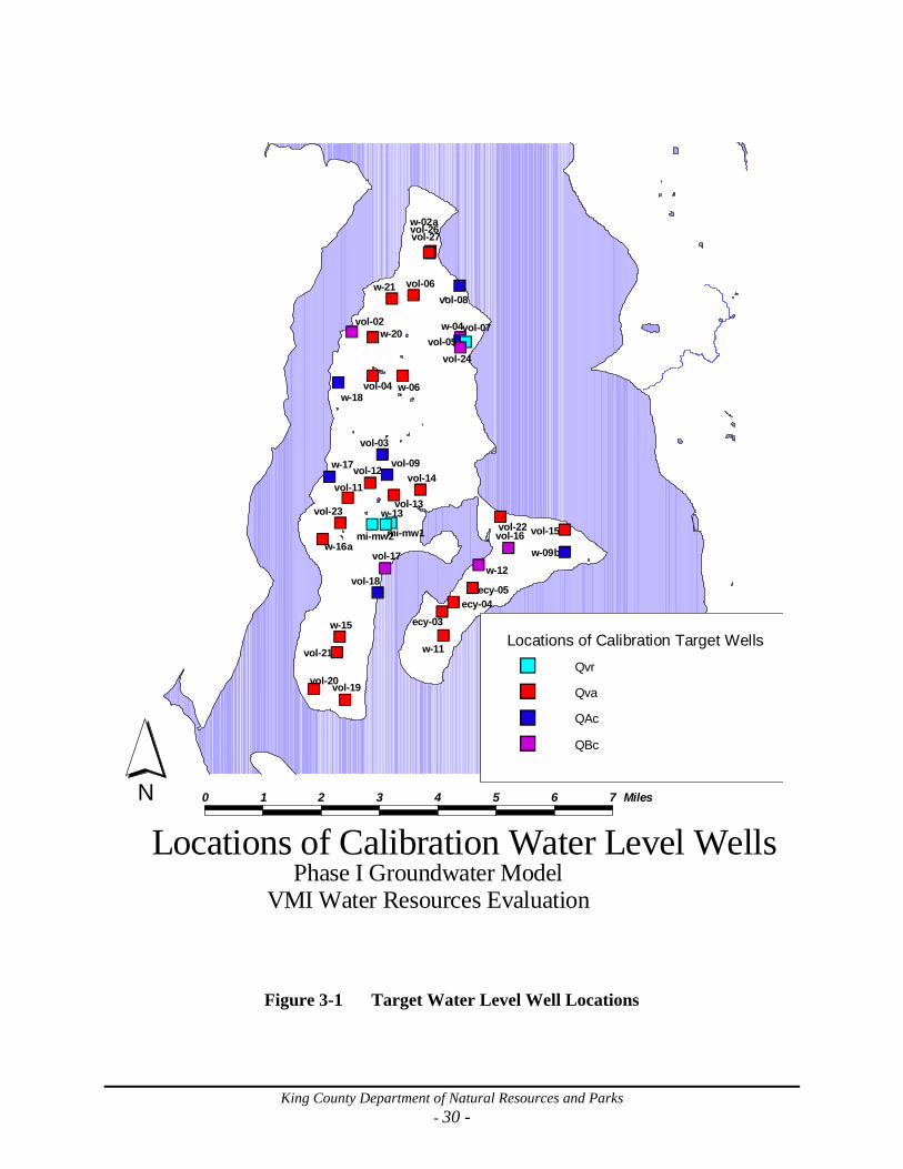
King County Department of Natural Resources and Parks - 30 -
Locations of Calibration Water Level Wells0 1 2 3 4 5 6 7 MilesN
%U
%U
%U
%U
%U
%U
%U
%U
%U
%U
%U
%U
%U
%U
%U
%U
%U
%U
%U
%U
%U
%U%U
%U %U
%U%U
%U
%U
%U%U
%U
%U%U
%U
%U%U
%U%U
%U
%U%U
w-04
w-06
w-11
w-12
w-13
w-15
w-17
w-18
w-20
w-21
w-02a
w-09bw-16a
vol-02
vol-03
vol-04
vol-05
vol-06
vol-07
vol-08
vol-09
vol-11vol-12
vol-13
vol-14
vol-15vol-16
vol-17
vol-18
vol-19
vol-21
vol-22vol-23
vol-24
vol-27
ecy-03ecy-04
ecy-05
mi-mw1
vol-20
vol-26
mi-mw2
Phase I Groundwater ModelVMI Water Resources Evaluation
Locations of Calibration Target WellsQvr%UQva%UQAc%UQBc%U
Figure 3-1 Target Water Level Well Locations

King County Department of Natural Resources and Parks - 31 -
Figure 3-2 Calibration Results: Model (calculated) vs. Target (observed)
The check of water levels against the calibration targets was mainly accomplished using Visual MODFLOW’s head calibration graph as part of its post-processing system. This module plots observed water level elevations against calculated (model) elevations. In addition, various statistical measures are also presented for the fit of the modeling run. This calibration plot is shown in Figure 3-2 for the final calibrated model. This run was considered the best possible fit to the target water levels, within the constraints set for the calibration process, and so it was considered to be the calibrated model. A better fit for each step in the calibration is by definition a tighter (higher) correlation and more accuracy on average (smaller residual). For the final calibration run shown in Figure 3-2, the correlation coefficient is 0.87, and the mean difference (residual) between observed and calculated heads is 4.5 feet. (Head is the water level elevation in a well.)

King County Department of Natural Resources and Parks - 32 -
The horizontal and vertical hydraulic conductivities that constitute the calibrated model are shown in Table 3-1.
Table 3-1. Calibrated Hydraulic Conductivities
Model Layer
number
Hydrogeologic name
General nature
Horizontal Hydraulic
Conductivity (KH) (ft/d)
Vertical Hydraulic
Conductivity (KV) (ft/d)
1 (part) Qvr, Qal Aquifer 10 1 1 (part),
2 Qvt Aquitard 0.25 0.005
3,4 Qva Aquifer 2.5 0.25 5,6 Qpf Aquitard 1 0.001, 0.005 7 QAc Aquifer 10 1 8 QBf Aquitard 1 0.005 9 QBc Aquifer 20 2 10 QC Aquitard 1 1
Some of the separate layers in the system are notably better or less well fit to their observed water levels. The worst of these, by layer, are:
• Layer 3 (upper part of Qva) has a mean residual of -46’ (the model calculates these wells’ heads values too low) and a correlation coefficient of only 0.58. These are the green triangles (upward pointing) in Figure 3-2.
• Layer 8 (QBf) has a mean residual of +49’ (the model calculated water levels too high) and a correlation coefficient of -0.49. These are the green diamonds in Figure 3-2.
Two wells are the most difficult targets to get a good fit: Vol14 and Vol19. Vol14 is located close to the middle of Vashon Island, in Layer 4 (Qva). It had a model-calculated head of 198 feet (elevation), much higher than the observed 87 feet – the downward pointing blue triangle is in the upper left quadrant of Figure 3-2. This well does not have a log, so the depth of the well is not confirmed. If it is actually screened deeper than was reported, the model would show a lower head elevation at this point. Vol19 is located at the southern (Tahlequah) end of Vashon Island, again in the Qva (Layer 3, upward pointing green triangle in the lower right quadrant). The model calculates 101 feet while the observation in this well is 228 feet. The well is located near the edge of the aquifer, and the steep slope of the water table probably makes the model estimation difficult. Other checks for the calibration are discussed in Section 4.0, including comparisons between:
• total stream flows from the boundary conditions with gaging data that has been collected (for the 2004-2005 time frame)
King County Department of Natural Resources and Parks - 33 -
• calculated water levels against previous understandings of water level contours and estimated flow directions (see the water levels in the Qva aquifer in Figure 4-5)
• spring (drain) boundary conditions locations and quantities against known spring locations (Figure 4-4)
An acknowledged limitation in the model as it is constituted was that only the highest layer of the model (numerical layer 1, including Qvr and Qvt) was allowed to drain and to have unconfined water table conditions. Other configurations of layer definitions were attempted, including allowing drying to occur throughout the Qvt, in the Qva aquifer, and attempting various solution procedures, rewetting parameters, and other modeling stratagems, but all were unsuccessful at correcting the problem with wetting in deeper layers. A possible reason (based on the locations for poor convergence) is that there is significant pumpage in the Qvr layer near the Burton wells, and this introduces an instability that cannot be overcome without modifying the stratigraphy of the model, at least in that area. Attempts at resolution of this inconsistency with the actual unconfined conditions required significant effort and could not correct the difficulty entirely. Other modeling efforts in the region (e.g., Van Heeswijk & Smith, 2002) have had similar difficulties and resolved them by just avoiding the issue by using only confined conditions, even in units at the ground surface. A proper modeling effort should confirm the adequacy of the calibration fit by observing the model’s prediction of a separate set of targets, over a separate set of inputs (e.g., a different time frame). This is called validation, and is designed to avoid relying too much on the particularities of a given calibration target data set. However, there was no separate validation dataset available, so that step in the modeling process had to be omitted.

King County Department of Natural Resources and Parks - 34 -
4.0 SIMULATION RESULTS This section discusses the results of the calibrated Phase I groundwater model. While much of the usefulness (and a purpose) of the modeling effort is a result of the creation of the datasets and the improved understanding of the hydrostratigraphy that have gone into the model development (see Section 1.0), there are demonstrations from the operation of the calibrated model that are discussed in this section. The first subsections discuss what the model indicates about the groundwater system on the Island and how well it reflects know aspects of the groundwater system, as demonstrated in the calibrated model (final calibration run). Some of the main issues that are of interest in this effort are:
• What are the fractions of the water balance that the various flow components contribute? (Sections 4.1, 4.2)
• What does the model show about groundwater flow directions? (Section 4.3) • How well do the data determine the calibration of the model (sensitivity analysis)?
(Section 4.4) The first two of these explicitly address the water balance and spatial distribution needs that were purposes of the model as discussed in Section 1.1. The sensitivity analysis is a normal step in model development (Figure 1) that helps guide the calibration and suggests appropriate efforts for subsequent investigation and modeling efforts on VMI. Later sections discuss the application of the model for predictive purposes. A simplified scenario that describes the effect of a 10% population increase, is included (in Section 4.6) as an illustration of the potential usefulness of the model.
4.1 COMPONENT WATER BALANCE The water balance is an accounting of the different components of the hydrologic cycle, as indicated by the steady-state modeling results. The water balance (Table 4-1 and Figure 4-1) for the calibrated model shows that:
• In input to the aquifer, precipitation recharge as expected provides the bulk (96%) of the water. The other components, septic systems (3%), and rivers and lakes (1%) add only a little.
• Among the water that leaves the aquifer, most (81%) goes out to Puget Sound via deep underwater springs. In the calibrated model, the streams (river boundary conditions) are next at 12% (of total aquifer flow), then wells (4%) and springs (drain boundary conditions) at 2%.

King County Department of Natural Resources and Parks - 35 -
Table 4-1 Inflows and Outflows in Model
Into aquifer Out from aquifer Recharge Precipitation, + 15,992 gpm
Septic systems: + 438 gpm Lakes: + 26 gpm
Total: + 16,455 gpm
Puget Sound - 13,501 gpm Streams
(base flow) + 239 gpm - 2,081 gpm
Wells Group A = -239 gpm Group B = -57 gpm
individual = -236 gpm Irrigation = -233 gpm
Total: - 765 gpm Springs - 360 gpm Total: + 16,694 gpm - 16,694 gpm
Note: spring discharges are included in model as drain boundary conditions, but could not be calibrated to, or even checked against, specific spring locations or flow quantities. These include -101 gpm of Group A springs sources and -4 gpm of Group B springs sources. Drinking water production for King County Water District 19 includes -168 gpm from stream sources. These quantities were not considered in the model.

King County Department of Natural Resources and Parks - 36 -
Figure 4-1 Water Balance Details (flows in gpm)
Note: Greater flows are shown with thicker arrows. Units without boxes at right of figure indicate flows out (negative) and into (positive)
aquifer unit, to and from streams (adjacent arrows). Table 4-2 compares the water balance components of the Phase I model to previous studies of Island hydrogeology, namely the study by Carr (1983) and that done for the Groundwater Management Plan (GWMP, VMI GWAC 1998). (Some components such as the breakdown between runoff and ET had to be calculated separately from the model, according to the USGS method of Bidlake and Payne, 2001.)
Qvr
Qvt
Qva
Qpf
QAc
QBf
QBc
QC
Recharge 16455
+803
+1565
Springs -360
Streams -1841
Puget Sound -13501
-360
-13501
780 24
16364 9
15647
9434 9019
2887 2592
2383 2197
243 242
Wells -753
-47 -50
-167
-200
-67
-35
-186
-1
-8 Qvt +4
-198 Qva +17
-1745 Qpf +214
-52 QAc +0
-78 QBf +4

King County Department of Natural Resources and Parks - 37 -
Table 4-2 Comparison of Model Water Balance to Previous Studies
VMI WRE Phase I GW model
(this report) Carr Report
(JR Carr/Assocs, 1983) Groundwater Management
Plan (VMI GWPC, 1998)
Inflows gpm % of precip
gpm % of precip
gpm % of precip
Precipitation 49,584 100% 48,851 100% 56,500 100% ET 21,410 43% 24,425 50% 22,370 40% runoff 11,719 24% 18,319 37% 13,170 23% GW inflow 16,455 33% 6,107 13% 20,960 37% Outflows Puget Sound 13,501 27% 1,224 3% 8,110 14% Streams 1,841 4% 4,882 10% 12,850 23% Wells 753 2% Springs 360 1% The model can be seen to be generally between other two estimates in the fraction of precipitation that goes to the different components. The major exception to this general observation is that the model sends a greater fraction to deep discharge to Puget Sound (27% compared to 3% and 14% for Carr and the GWMP). It also sends correspondingly less flow out to streams as base flow (4% compared to 10% and 23%). (Note that these percentages are of the total precipitation and are thus on a different basis from those in the preceding paragraph, which are percentages of total recharge only.)
4.2 STREAMS AND SPRINGS Streams: During the calibration process, stream boundary conditions were considered only in qualitative way. The field data for three Island-wide stream-gaging surveys were compared to model results generally, as shown in Figure 4-2. The outflow or inflow for each of the boundary condition cells that were part of a given river system were compiled and added up algebraically. This was done without consideration of whether there could have been any streamflows in the upland stream reaches to allow seepage into the aquifer. The upland losing stream segments are dry in the summer and thus cannot physically contribute to the downstream base flows during dry periods when field work can measure them, but must be included as part of the year-round steady-state operation of the aquifer system that is being modeled. The summed stream flow quantities are compared in Figure 4-2 with the averaged (geometric mean) observed stream flows.

King County Department of Natural Resources and Parks - 38 -
0.01
0.1
1
10
0.01 0.1 1 10Gage flows (cfs)
Tot
alle
d M
odel
Flo
ws (
cfs)
Figure 4-2 River flows: Gauged Data vs. Model Totals
Figure 4-2 shows that the streams are fairly well represented in the model in their total, despite gross simplifications such as having all the river boundary conditions with the same conductance despite their underlying geologic stratum, the water level in the stream, its length across a model cell, or any of the other aspects of reality that could have been considered in the imposition of this boundary condition. The model totals are approximately 60% of the averaged flows that have been measured in the field, with the relationship somewhat more accurate for the smaller streams than for the larger ones. The agreement is actually better than appears at first, because the model was calibrated with recharge for normal (1961-1990) precipitation, while the gaged data are for present day (2004-2005) measurements when the precipitation has been lower. Also, summer baseflows, when these are measured, may be somewhat less than year-round discharges from aquifers to streams. The groundwater model predicts only baseflow; whereas, the gauges measure all flow (baseflow and runoff and interflow, which is flow from the near stream shallow soils). So it is reasonable that model predictions would be lower than gauge measurements. Note that this streamflow comparison was checked during the calibration effort but not used significantly for choosing the changes in parameters for calibration – agreement with target

King County Department of Natural Resources and Parks - 39 -
water levels was the sole criterion for fitness of calibration. Thus, the agreement on the streamflows could be improved but only by accepting less accuracy in fitting groundwater levels. The locations and quantities of stream / groundwater interactions as calculated by the groundwater model are shown in Figure 4-3. As expected, along the upper portions of the streams the streambeds are above the groundwater and the streams lose water to the groundwater in these reaches (pink squares). There are a few stream flow totals that could not be shown in Figure 4-2 because the model calculated them to be entirely losing and a negative flow cannot be included in a log scale plot. These negative flow streams include Chen, Mileta, and Glen Acre Creeks. Outflows are found mostly at the lowest reaches of the streams, near their outlets to the Sound. The largest outflows are near the mouth of Judd Creek, Shinglemill Creek, and a few others. The streams flowing to Colvos Passage to the west tend to have higher groundwater discharges, disproportional to their relatively small catchment areas. Springs: Discharges to springs (drain boundary conditions), as estimated in the calibrated model, are shown in Figure 4-4. The reported locations of actual (or historical) springs are also shown in the Figure. There is reasonable agreement about locations: the cells that release water via the drains are distributed similarly to the reported springs, although some inland locations such as along Judd Creek valley appear more limited in the model than in real life. The quantities of spring flows appear to be estimated somewhat low in the model, judging only on estimated springs flow as used by some Group A water systems. Some of these Public Water Systems rely on spring sources for production quantities that may range up to about 50 gpm, while the model drain cells do not have flows per cell of more than about 7 gpm. Some of these springs sources are found at very local low areas and are further enhanced by infiltration galleries, which effectively lower the drain level at the spring. The drain boundary condition in the model, on the other hand, is based on ground surface elevation at the center of the model cell. If data were available to model these very local conditions, the springs flows could be better estimated. Even at higher flow rates, however, it is unlikely that the springs would constitute a major component of the overall groundwater system. Like the stream flows, spring flows were checked during the calibration process but not used in the calibration process.

King County Department of Natural Resources and Parks - 40 -
0 1 2 3 4 5 6 Miles
NModel Predicted Stream Gains and Losses
Phase I Groundwater ModelVMI Water Resources Evaluation
Stream boundary flowslosing (58 cells)
gaining:
< 5 gpm (3 cells)
5-15 gpm (16 cells)
15-30 gpm (16 cells)
30-45 gpm (11 cells)
45-60 gpm (13 cells)
> 60 gpm (7 cells)
Figure 4-3 River Boundary Condition Locations and Flows

King County Department of Natural Resources and Parks - 41 -
0 1 2 3 4 5 6 Miles
NModel Predicted Spring Flows
Phase I Groundwater ModelVMI Water Resources Evaluation
%a
%a
%a
%a
%a%a%a
%a
%a
%a
%a%a%a%a
%a
%a
%a
%a
%a
%a
%a
%a
%a
%a%a%a
%a
%a%a
%a
%a%a
%a%a%a
%a
%a%a
%a %a %a%a
%a
%a
%a
%a%a
%a
%a
%a
%a
%a
%a
%a
%a
%a
%a
%a%a%a%a%a%a
%a
%a %a
%a%a%a%a
%a
%a
%a
%a
%a%a%a%a %a
%a
%a
%a%a
%a%a
%a
%a
%a%a
%a
%a%a%a
%a%a
%a
%a %a
%a %a
%a
%a%a%a%a
%a
%a
%a%a%a
%a%a
%a
%a
%a
%a
Spring boundary flowsdry (64 cells)
< 1 gpm (29 cells)
1 - 2 gpm (35 cells)
2 - 3 gpm (34 cells)
3 - 4 gpm (26 cells)
4 - 5 gpm (14 cells)
> 5 gpm (8 cells)
Reported Spring Location%a
Figure 4-4 Spring Boundary Condition Locations and Flows
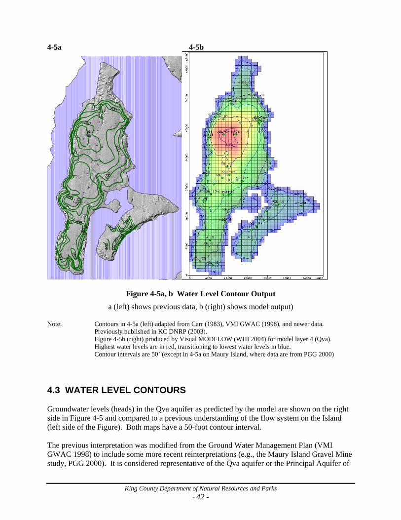
King County Department of Natural Resources and Parks - 42 -
4-5a 4-5b
50
100
150
20040
20
3060
25070
300
50
200
50
100
200
250
150
250
Figure 4-5a, b Water Level Contour Output a (left) shows previous data, b (right) shows model output)
Note: Contours in 4-5a (left) adapted from Carr (1983), VMI GWAC (1998), and newer data.
Previously published in KC DNRP (2003). Figure 4-5b (right) produced by Visual MODFLOW (WHI 2004) for model layer 4 (Qva).
Highest water levels are in red, transitioning to lowest water levels in blue. Contour intervals are 50’ (except in 4-5a on Maury Island, where data are from PGG 2000)
4.3 WATER LEVEL CONTOURS Groundwater levels (heads) in the Qva aquifer as predicted by the model are shown on the right side in Figure 4-5 and compared to a previous understanding of the flow system on the Island (left side of the Figure). Both maps have a 50-foot contour interval. The previous interpretation was modified from the Ground Water Management Plan (VMI GWAC 1998) to include some more recent reinterpretations (e.g., the Maury Island Gravel Mine study, PGG 2000). It is considered representative of the Qva aquifer or the Principal Aquifer of

King County Department of Natural Resources and Parks - 43 -
Carr (1983). It was previously published as (part of) Figure 2 in the 2002 Groundwater Protection Program Annual Report (King County DNRP 2003). Many of the features that were included in previous interpretation show up in the model output. These include the steep groundwater gradients, particularly on the western edge of the Island. Some of the detailed features, such as the effect of the Judd Creek valley, do not show up prominently in the model. A mapping of the model output along the same Row 43 cross-section that was shown in Figure 2-2 (above) is presented here as Figure 4-6. The red squares in the figure show locations of fixed head boundary conditions, gray squares are drain boundary conditions (springs), and blue squares are river boundary conditions (streams). Cells that have dried out are shown in an olive color, and some vertical lines through the cells are target water level wells (with identification annotation also shown).
Figure 4-6 Cross-Section Graphical Output
Note: Output from Visual MODFLOW (WHI 2004) for model row 43.
Blue contours are water levels (potentiometric) at 50-foot intervals. Red vectors show flow directions. Red cells are fixed head boundary conditions. Dark blue cells are river boundary conditions. Light blue - green cells are portions of cells that are dry above water table (heavy blue line). Solid cells in middle are inactive cells beneath Quartermaster Harbor. The flow through this cross section is indicated by the equipotential lines (in blue) as well as by the flow vectors (red arrows) calculated by Visual MODFLOW. It shows, for example, that flows from the Vashon Island uplands flow out slightly more to the Colvos Passage to the west, rather predominantly to Quartermaster Harbor (the low area in the center) as would be indicated by surface water systems. This explains an observation of the stream flow survey data, that the
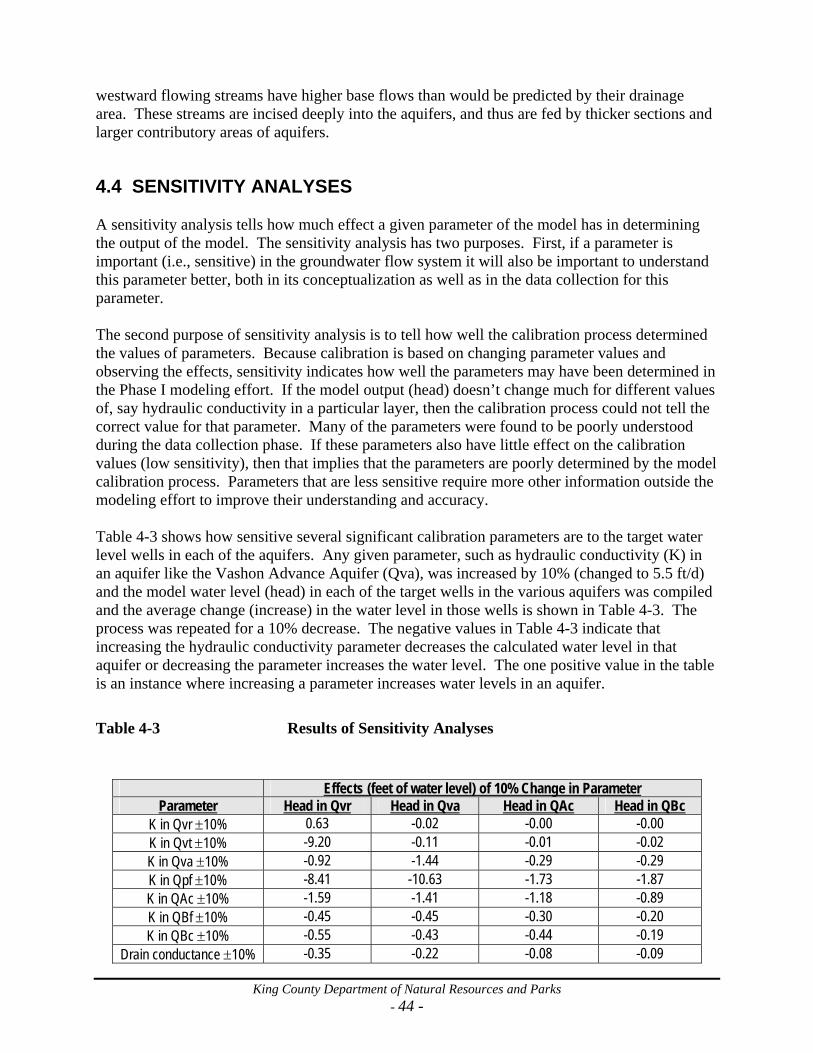
King County Department of Natural Resources and Parks - 44 -
westward flowing streams have higher base flows than would be predicted by their drainage area. These streams are incised deeply into the aquifers, and thus are fed by thicker sections and larger contributory areas of aquifers.
4.4 SENSITIVITY ANALYSES A sensitivity analysis tells how much effect a given parameter of the model has in determining the output of the model. The sensitivity analysis has two purposes. First, if a parameter is important (i.e., sensitive) in the groundwater flow system it will also be important to understand this parameter better, both in its conceptualization as well as in the data collection for this parameter. The second purpose of sensitivity analysis is to tell how well the calibration process determined the values of parameters. Because calibration is based on changing parameter values and observing the effects, sensitivity indicates how well the parameters may have been determined in the Phase I modeling effort. If the model output (head) doesn’t change much for different values of, say hydraulic conductivity in a particular layer, then the calibration process could not tell the correct value for that parameter. Many of the parameters were found to be poorly understood during the data collection phase. If these parameters also have little effect on the calibration values (low sensitivity), then that implies that the parameters are poorly determined by the model calibration process. Parameters that are less sensitive require more other information outside the modeling effort to improve their understanding and accuracy. Table 4-3 shows how sensitive several significant calibration parameters are to the target water level wells in each of the aquifers. Any given parameter, such as hydraulic conductivity (K) in an aquifer like the Vashon Advance Aquifer (Qva), was increased by 10% (changed to 5.5 ft/d) and the model water level (head) in each of the target wells in the various aquifers was compiled and the average change (increase) in the water level in those wells is shown in Table 4-3. The process was repeated for a 10% decrease. The negative values in Table 4-3 indicate that increasing the hydraulic conductivity parameter decreases the calculated water level in that aquifer or decreasing the parameter increases the water level. The one positive value in the table is an instance where increasing a parameter increases water levels in an aquifer.
Table 4-3 Results of Sensitivity Analyses
Effects (feet of water level) of 10% Change in Parameter
Parameter Head in Qvr Head in Qva Head in QAc Head in QBc K in Qvr ±10% 0.63 -0.02 -0.00 -0.00 K in Qvt ±10% -9.20 -0.11 -0.01 -0.02 K in Qva ±10% -0.92 -1.44 -0.29 -0.29 K in Qpf ±10% -8.41 -10.63 -1.73 -1.87 K in QAc ±10% -1.59 -1.41 -1.18 -0.89 K in QBf ±10% -0.45 -0.45 -0.30 -0.20 K in QBc ±10% -0.55 -0.43 -0.44 -0.19
Drain conductance ±10% -0.35 -0.22 -0.08 -0.09

King County Department of Natural Resources and Parks - 45 -
River conductance ±10% -0.61 -0.32 -0.29 -0.08 It can be seen in this analysis that increasing the conductivity generally allows more water to flow out of the model, and so the heads drop. In the single contrary situation, increasing the conductivity in the Qvr increases the water levels in the same aquifer, presumably because the change attracts other flows into this unit. The sensitivity analysis also shows that the most sensitive parameters (based on their average absolute change in head in these aquifers) are:
• K in Qpf aquitard • K in Qvt aquitard • K in QAc aquifer • K in Qva aquifer
The first two of these parameters (K in Qpf and QAc) are probably especially sensitive because they connect the aquifers to the important outflow boundary condition that allows water to exit to Puget Sound. This boundary condition could not be independently evaluated in the sensitivity analysis process. The sensitivity of these parameters indicates that this boundary condition should be reassessed and possibly reconfigured in subsequent phases of modeling. The sensitivity of all these parameters shows how important the conductivity values are in these shallow aquifers and aquitards. Subsequent investigations will include pumping testing of the Qva aquifer. The least sensitive parameters are:
• K in Qvr aquifer • Conductance in drain (springs) boundary conditions • Conductance in river (stream) boundary conditions • K in QBf aquitard • K in QBc aquifer
The drain (springs) and river (streams) boundary conditions show up as relatively insensitive, as adjusted by their conductance parameters, so these boundary conditions are probably not well determined by the modeling effort. The effect of correcting the elevations associated with these boundary conditions could not be readily included in the sensitivity analyses, and may be more critical (sensitive) than the conductance values. Finally, the flows to these boundary conditions were not used to judge the accuracy of the calibration, and flows are probably more sensitive to the boundary condition parameters (conductance and elevation). Modeling the surface water - groundwater interactions could result in a better understanding of the Island’s hydrology. The above sensitivity analysis is expressed in terms of the effects from hydraulic conductivity, but the parameter in the model is actually a combination of the thickness of the unit and its hydraulic conductivity (referred to as transmissivity). So, the sensitivity analysis also indicates the importance of accurate hydrostratigraphy. It is very important that the thickness of the lower (pre-Fraser) glacial aquifer (QAc) be delineated better, because the solution is very dependent on

King County Department of Natural Resources and Parks - 46 -
the overall effect of its thickness and hydraulic conductivity. Similarly, the importance of K in the aquitards demonstrates that “windows” in these units (places where the unit may be absent) can be very significant to the water levels, and getting this aspect of the hydrostratigraphy accurate will be important in future studies. The sensitivity analysis was accomplished by changing the hydraulic conductivity for both horizontal and vertical directions. However, in aquitards, the vertical hydraulic conductivity governs the flow more than horizontal, and opposite for horizontal conductivity in aquifers. The importance of the vertical conductivity values (note that the Qpf aquitard is the most sensitive layer) also highlights the difficulty of measuring this aquifer property accurately by field activity. There are other aspects that could be included in this sensitivity analysis (e.g., agricultural pumpage was also not well understood), but since the parameters included in the sensitivity analysis were the one that were used for the calibration, the sensitivity analysis was considered adequate with just these comparisons. The sensitivity analysis can also be used on a local basis – are there particular areas of the Island where a particular parameter should be studied in more detail? should some parameters be calibrated with variations allowed over smaller areas (zones in MODFLOW terminology)? are the water level data more determinate in the calibration in one area compared to another? These issues will be dealt with during subsequent phases of modeling and investigation.
4.5 GAIN IN UNDERSTANDING A major objective for the development of the Phase I Groundwater Model (Section 1.2) was to improve the understanding of the aquifer systems on Vashon-Maury Island. What kinds of improvements in understanding have been made possible with the development of this model? One illustration of the facility that the model provides is that the Phase I model considers deeper aquifers, rather than just the Qva (or Principal Aquifer), as has been the focus for many previous studies. The Phase I model has incorporated these deeper aquifers in a relatively simplified form, due to the limited information available about these systems. An example of a question about the deeper aquifers that can be viewed via the model is the vertical gradient. It has been observed that the static groundwater levels (heads) demonstrate a downward gradient (lower heads the deeper one drills). This is a significant issue for Vashon-Maury Island because it is a demonstration that there is no off-Island source of water (which would show up as an upward gradient). The Visual MODFLOW post-processing system allows output of head difference, rather than gradient, but this parameter is indicative of the gradient (upward or downward). Figure 4-7 shows that the two main aquifers (Qva and QAc) show a downward gradient virtually everywhere on the Island. The exception to this general rule is along the coastline, which is probably an effect of the constant head boundary condition.

King County Department of Natural Resources and Parks - 47 -
4.6 PREDICTIVE RUNS One of the main issues that should be addressed by the modeling effort is what would happen if conditions changed. While there are many limitations in the model, it is appropriate to demonstrate the capability of the model in this regard and to present some preliminary results. Predictive runs allow the potential impacts of various scenarios to be evaluated. This is done by adjusting Boundary conditions according to the scenario considered. For example, the impact of population growth can be considered by increasing the pumpage in the model, or climate change can be considered by changing the recharge, and so on. To consider the possible effect of increased population in a simplified scenario, the model was run with the flows in all the water supply wells increased by 10%. This includes the Group A wells (Section 2.4.1.1); Group B wells (2.4.1.2); and individual wells (2.4.1.3). Since it was considered that this water supply was for population increase, the recharge due to septic drain fields (Section 2.4.3) was also increased by 10%. Similarly, the flows in agricultural irrigation (Section 2.4.1.4) wells were not changed. The result of this simulation run is shown for layer 4 in Figure 4-8 (plan view over entire Island) and along a cross-Section at Row 43 in Figure 4-9 (the same cross-Section shown in previous figures). In these Figures, areas with drawdown are shown warmer colors (e.g., red and yellow) and areas with higher water levels are shown in cooler colors (blue). There are also red contour lines at an interval of 0.5 feet, although many of the contour lines in the two Figures are simply separating areas of increase and decrease (0’ drawdown contour line). The two figures show the increased pumpage of wells belonging to Group A systems (e.g., Burton, Gold Beach, and Heights) have a noticeable effect. The effect near Burton shows up in the plan view (Figure 4-8) of layer 4 even though the increased pumpage actually occurs in layer 1. However, the colors are more dramatic than the numerical values would indicate: the maximum drawdown over the entire model is about 5 feet, in the area around the Burton well field. The areas of higher water level due to increased septic return flows, shown as blue areas in the Figures, have a maximum rise of about 1.6 feet, in the downtown Burton area.

King County Department of Natural Resources and Parks - 48 -
Figure 4-7 Model-Estimated Head Difference Between Qva and QAc Aquifers
Notes: - Difference in head between model layer 4 and layer 7 (Qva - QAc) as shown in Visual
MODFLOW output (WHI, 2004). - Blue areas are areas with a downward gradient, yellow to red areas have upward gradients. Contour intervals are 20 ft of head difference. - Does not show gradient value directly, which would include thickness of aquitard.

King County Department of Natural Resources and Parks - 49 -
Figure 4-8 Drawdown for Increased Pumpage (Layer 4, plan view) Note: Red areas show drawdown; blue indicate water level rise; green are intermediate.

King County Department of Natural Resources and Parks - 50 -
Figure 4-9 Drawdown for Increased Pumpage (Model Row 43)
Note: Red areas show drawdown; blue indicate water level rise; green are intermediate. This predictive simulation is illustrative rather than precise. It shows that the model can indicate future behavior of the aquifer system according to an imposed scenario. The particular scenario used here is not realistic: obviously a real population increase would not result in the same percentage flow increase in all the same (existing) wells. Moreover, a suitable data set of different water levels or during a period of different pumpage in the specific vicinity that could bracket these conditions (i.e., a validation dataset) is lacking. Similarly, water level information in the areas of concern is also scarce. These factors limit the predictive value of the scenario. Other scenarios are readily performed. Changes due to climatic changes can be imposed by increasing or decreasing the precipitation-related recharge. Changes due to changes in surface water management (e.g., low impact development leading to greater infiltration) can be modeled by localized increased recharge. However, these predictive scenarios are probably better run after the model is peer reviewed or after subsequent phases of model development.

King County Department of Natural Resources and Parks - 51 -
5.0 RECOMMENDATIONS FOR SUBSEQUENT WORK This Section provides some guidance for future phases of groundwater modeling of the Vashon / Maury Island aquifer system, as learned through the preparation, calibration, and operation of the Phase I model. It also provides suggestions for investigation, to address data gaps that were found to be limiting to the modeling effort.
5.1 HYDROSTRATIGRAPHY One of the main constraints of the present modeling effort is gaps in knowledge of the stratigraphy of Vashon-Maury Island. As good as the 3-D mapping that UW’s GeoMapNW research center performed, it was limited by the availability and accuracy of the existing data. For the most part, these data were obtained from drillers’ logs for water wells, and these are limited by the lack of down-hole sampling during the drilling of the wells. In addition, the accuracy of the locations of these wells is poor – the township / range / Section / quarter-quarter Section are often misreported, and addresses are omitted or reported only as postal addresses. Some of this problem has been addressed (by GeoMapNW) by trying to connect the name of the well owner on the log with the ownership of parcels in the area, although even this does not work for former residences. Additional corrections could be obtained by consulting Vashon residents for their knowledge. In addition, some reinterpretation of the hydrostratigraphy was obtained only after the model layers had to be finalized, as many other features (such as boundary conditions) depend on the specified layering. During subsequent phases of the modeling, these reinterpretations can be considered. Improvements in the location of wells on the Island will also have the benefit of providing better estimates of pumping well boundary conditions. Drilling monitoring wells on the Island will also provide additional information that will inform models during later phases. It is important to obtain, preserve, and document samples of the subsurface during this drilling, so that the descriptions of the strata can be checked later under less time constraints.
5.2 AQUIFER PROPERTIES A significant limitation to this modeling effort was the lack of sufficient direct measurements of aquifer properties, specifically hydraulic conductivity. During the model development, requests for documentation of any additional testing were made but few surfaced in this process. The new monitoring wells will be used for pumping tests that will provide an accurate measure of these parameters, at least in the vicinity of the wells. Ideally, they should be placed in areas of the Island where few tests have been conducted previously. The hydrostratigraphy throughout the Puget Sound region is complicated by the dynamic depositional environments that the glaciers created during the placement of these layers, and

King County Department of Natural Resources and Parks - 52 -
these small features cannot be readily discerned in the drilling record or portrayed in a regional-scale model. An illustrative example of how complicated the stratigraphy turns out to be, when an area is studied closely, is the study of the former Vashon landfill (Berryman & Henigar, 2004). In response to this complication is the realization that it may be possible and necessary to use more of this data and lump the various components of the aquifer (clay layers and sand layers, saturated and unsaturated) into a composite set of aquifer properties for a given zone. Another aspect regarding aquifer properties that should be included in subsequent phases of groundwater modeling is to vary an aquifer property across the extent of the Island. It is likely that the Qva aquifer (for example) is coarser in one part of such a large area than in another. Some consideration of such variability should be included in the model calibration. This was not done for the Phase I model because there was no data regarding such variability, to guide the selection of such zones and to estimate their initial differences in hydraulic conductivity. It will be necessary to check such geographic variations (e.g., through a spatial analysis of stratigraphic descriptions, or some sedimentation analysis of the glacial depositional process). Another related aquifer property question is rather computational rather than physical: Only layer 1 of the model (Qvr and portions of Qvt) could be specified as unconfined or allowed to drain out to unconfined conditions or even to completely dry. However, it is known that some areas of Qva (layers 3 and 4 in the model) actually also show unconfined conditions. In MODFLOW this condition can be applied only throughout an entire layer, but when this was tried, the model could not converge, despite attempting variations in solvers or settings. (This is apparently a common problem that is encountered with modeling in this region, as found in other groundwater models in the Puget Sound region; e.g., Van Heeswijk & Smith, 2002.)
5.3 GRID SPACING A model is a simplification of reality and the more it departs from reality the less accurate it is expected to be. One of the most obvious simplifications is the grid sizing. If the grid spacing is made finer, the model will be better in several ways: boundary conditions can be placed more precisely, the effects of boundary conditions can be distanced from areas of concern, and the stratigraphy can be entered with more detail. The grid spacing has to be set early in the model development, and changing the grid affects other data sets that rely on the grids so complicates the modeling process. With the rapid advances in computational force in recent years it is now possible to create and exercise models of greater magnitude and complexity than could be considered even relatively recently. Some of the data sets for these extensive or complicated models can be derived through automated processes such as grid interpolation using programs like Surfer (Golden Software, 2002) and GIS processing of data sets like LiDAR. There are still limitations in the derivation of some boundary conditions, such as river bed / water surface elevations, that have not been developed in the past and initially require very precise and manual interactions that cannot easily be scaled to the more complicated model. This constraint also applies in general to the input to the model of detailed refinements of the hydrostratigraphy. Creativity and computational skill are needed to develop automated approaches to make more detailed modeling possible.
King County Department of Natural Resources and Parks - 53 -
Some issues of concern on the Island, such as localized issues of lateral flow or contaminant transport will require more detailed grid and subdomain modeling.
5.4 BOUNDARY CONDITIONS Boundary conditions have limitations both in knowledge of reality as well as their implementation in the model. A major uncertainty is the amount of recharge. Since this phenomenon sets the basic amount of water that is available for the model to transport to the various users and discharge points for the water. For the purposes of the Phase I model a regionally-based regression estimate of recharge (Bidlake and Payne, 2001) was applied, using accurate land use and refined surficial geology but also regional estimates of precipitation and implicit regional assumptions of evaporation and transpiration. Further refinements of the precipitation zones will help to create a better recharge distribution on the Island. There are questions about the estimates that were used for well pumpage, particularly for agricultural. Improving this estimate will probably have to await a requirement for metering flows, either generally or for specific water right or exempt wells. Limited metering (i.e., at only a few wells) will probably affect usage of those observed wells and thus give a biased estimate of general pumpage rates. Surface water / groundwater interaction, and the recharge issues mentioned above, may be better defined by surface water modeling. There are inconsistencies in the approaches, theoretical bases, and data utilization between surface water modeling and groundwater modeling. These differences make it difficult to combine the two methods into an integrated modeling approach to the Island, although this issue is being investigated for Phase 2 implementation. Another boundary condition that should be considered for improvement is the interface of the model with Puget Sound. This constant head boundary is required for proper model functionality. In the Phase I model the boundary was placed immediately adjacent to the active areas on the Island, but placed in an aquitard (Qpf) to set it at the appropriate level and to provide some hydraulic distance from the rest of the model. It may be possible to set this boundary more off shore and provide it with a separate, adjustable conductance (e.g., a separate hydraulic conductivity zone), that will together allow it to accurately model this important connection, be included in the calibration / sensitivity parameters, and perhaps even account for the salt water interface issue.
5.5 TRANSIENT FLOW CONDITIONS Some important issues for consideration by modeling can only be addressed by running a model in a transient mode rather than the steady state condition used for this Phase I model. Some of these issues are:

King County Department of Natural Resources and Parks - 54 -
• seasonal fluctuations • short term water level response from drought conditions • simulation of impacts from new pumping wells (including simulation of pumping tests) • summer low flows in streams
Difficulties for running the model in this way include the need to estimate boundary conditions appropriate for transient conditions, as well as appropriate calibration targets. The recharge boundary condition is especially problematic because it has been observed previously (Carr 1983) that precipitation at the ground surface can take months to reach the water table and become recharge. As an example of the difficulty: the only previous groundwater flow model for a portion of the Island (PGG 2000) attempted to route recharge lag through the unsaturated zone to feed into a transient model. They found that this approach was not feasible, mainly due to a limited calibration data and the variability of response parameters.
5.6 CALIBRATION / VALIDATION DATA A definitive groundwater model should include a separate calibration target. This was not possible in the Phase I effort because of the limited number of water level data points (locations and number of values). It could be possible to do a reduced form of validation (more of a check of the calibration) by comparing the model results at the larger set of data that is not well located, has a limited number of measurements, or where the observations were taken some time in the past. This was not even attempted, because the likely low correlation could not be determined to be the consequence of a poor model calibration rather than the poor quality or representativeness of the data. To obtain an improvement in a next phase model it is vital to obtain greatly improved calibration (and validation) data. Some of this should be obtained by continuing the existing volunteer water level program (even if on an occasional rather than continuous monthly basis). Another contribution may come from instrumenting some Group A wells. For these data to be useful for calibration will be necessary to meter pumpage rates simultaneously with the water levels, to allow extraction of static water levels from the dynamic levels that will be measured. Finally, although not formally calibration data, it will be useful to future modeling efforts to improve the mapping (and obtain flow measurements) of springs across the Island, and to continue the stream flow measurements. These data provide a valuable check on the model results.

King County Department of Natural Resources and Parks - 55 -
6.0 REFERENCES
AGI Technologies. 1997a. Morgan Hill Test Well – Construction and Testing Report – King County Water District No. 19. January 7, 1997.
AGI Technologies. 1997b. Gerrior Test Well – Construction and Testing Report – King County Water District No. 19. August 25, 1997.
Berryman & Henigar. 2004. Vashon Island Landfill – Hydrogeologic Report Update. In association with Udaloy Environmental Services. Prepared for DNRP, Solid Waste Division. December 2004
Bidlake, W.R., and Payne, K.L. 2001. Estimating recharge to groundwater from precipitation at Naval Submarine Base Bangor and vicinity, Kitsap County, Washington. U.S. Geological Survey Water-Resources Investigations Report 01-4110, 33 p. [also available via: http://wa.water.usgs.gov/projects/bangor/publications.htm]
J.R. Carr / Assocs. 1983. Vashon / Maury Island Water Resources Study. Submitted to the King County Dept of Planning and Community Development. December 1, 1983.
Carr/Assocs Inc. 1990. Report on the Construction and Testing of Production Well 2 for King County Water District 19. May 24, 1990.
Carr/Assocs Inc. 1992. Production Well 1 – Construction and Testing Report – Maury Mutual Water Company. June 11, 1992.
CDM. 2004. Biannual Nitrate Monitoring Summary Report (January 2004 – June 2004); Development Services of America, Misty Isle Farms, Vashon Island, Washington. June 18, 2004.
Cox, Stephen E. and Sue C. Kahle. 1999. Hydrogeology, Ground-Water Quality, and Sources of Nitrate in Lowland Glacial Aquifers of Whatcom County, Washington, and British Columbia, Canada. US Geological Survey, Water-Resources Investigations 98-4195.
Garling, M.E., Dee Molenaar, et al. 1965. Water Resources and Geology of the Kitsap Peninsula and Certain Adjacent Islands. Washington Division of Water Resources, Water Supply Bulletin No. 18. With contributions by the US Geological Survey. (also available at http://www.ecy.wa.gov/programs/eap/wsb/wsb_Hydrologic-Systems.html)
Golden Software, Inc. 2002. Surfer User’s Guide. Golden, CO.
Harbaugh, A.W., Banta, E.R., Hill, M.C., and McDonald, M.G. 2000. MODFLOW-2000, the U.S. Geological Survey modular ground-water model – User guide to modularization concepts and the Ground-Water Flow Process. U.S. Geological Survey Open-File Report 00-92, 121 p. [Also available via http://water.usgs.gov/nrp/gwsoftware/modflow2000/modflow2000.html]
King County Department of Natural Resources and Parks - 56 -
Kahle, S.C. 1998. Hydrogeology of Naval Submarine Base Bangor and Vicinity, Kitsap County, Washington. Water-Resources Investigations Report 97-4060.
King Co DNRP. 2003. King County Groundwater Protection Program – 2002 Annual Report. April 1, 2003. [also available via http://dnr.metrokc.gov/wlr/wq/2002-groundwater-report.htm]
King Co DNRP. 2004. Vashon-Maury Island Rapid Rural Reconnaissance. July 2004. [also available via http://dnr.metrokc.gov/wlr/rural-drainage-program/vashon-projects-2004.htm]
King Co DNRP. 2005. Vashon-Maury Island Watershed Plan. June 6, 2005. [also available via http://www.vmicc.org/media/Vashon_Plan.pdf]
McDonald, Michael G., and Arlen W. Harbaugh. 1988. A Modular Three-Dimensional Finite-Difference Ground-water Flow Model. United States Geological Survey. Techniques of Water-Resources Investigations, Book 6, Chapter A1, 586 pp. [also available via http://water.usgs.gov/nrp/gwsoftware/modflow2000/modflow2000.html]
National Groundwater Association (NGWA), 2004, The New MODFLOW Course, Course notebook and reference materials, October 25-28, 2004, Princeton, New Jersey.
Pacific Groundwater Group (PGG). 2000. Maury Island Gravel Mine Hydrogeologic Impact Assessment. Prepared for Washington State Dept of Ecology. Ecology Publication 00-10-026. May 2000.
Rongey and Assocs. 1992. Heights Water Corporation – Construction & Testing, Well No. 3. Nov. 20, 1992.
Turney, G.L., S.C. Kahle, and N.P.Dion. Geohydrology and Ground-Water Quality of East King County, Washington. Water-Resources Investigations Report 94-4082. Prepared in cooperation with Seattle - King County Dept. of Public Health. Tacoma. 1995
Van Heeswijk, Marijke, and Smith, D.T., 2002, Simulation of the ground-water flow system at Naval Submarine Base Bangor and vicinity, Kitsap County, Washington. U.S. Geological Survey Water-Resources Investigations Report 02-4261, 142 p. [also available via: http://wa.water.usgs.gov/projects/bangor/publications.htm]
Vashon-Maury Island Groundwater Advisory Committee (VMI GWAC). 1998. Vashon-Maury Island Ground Water Management Plan. Supplement 1 – Area Characterization. Prepared by King County DNR and Seattle-King County Dept of Public Health. Final, submitted December 1998.
Waterloo Hydrogeologic Inc.(WHI). 2004. Visual MODFLOW v.4.0 User’s Manual. Waterloo, Ontario.
Woodward, D.G., F.A.Packard, N.P.Dion, and S.S. Sumioka. 1995. Occurrence and Quality of Ground Water in Southwestern King County, Washington. Water-Resources Investigations Report 92-4098. Prepared in cooperation with: State of Washington Dept.

King County Department of Natural Resources and Parks - 57 -
of Ecology, Regional Water Association of South King Co., and Seattle – King County Dept. of Public Health. Tacoma.